Embed Size (px)
Citation preview
sensors
Article
Assessment of Centre National d’Études SpatialesReal-Time Ionosphere Maps in Instantaneous PreciseReal-Time Kinematic Positioning over Medium andLong Baselines
Dariusz Tomaszewski 1,* , Paweł Wielgosz 1 , Jacek Rapinski 1 ,Anna Krypiak-Gregorczyk 1 , Rafał Kazmierczak 1 , Manuel Hernández-Pajares 2 ,Heng Yang 2 and Raul OrúsPérez 3
1 Faculty of Geoengineering, University of Warmia and Mazury in Olsztyn, Oczapowskiego str. 2,10-719 Olsztyn, Poland; [email protected] (P.W.); [email protected] (J.R.);[email protected] (A.K.-G.); [email protected] (R.K.)
2 Department of Mathematics, UPC-IonSAT & IEEC-UPC, Universitat Politècnica de Catalunya,08034 Barcelona, Spain; [email protected] (M.H.-P.); [email protected] (H.Y.)
3 ESTEC, European Space Agency, 2200 AG Noordwijk, The Netherlands; [email protected]* Correspondence: [email protected]
Received: 16 March 2020; Accepted: 15 April 2020; Published: 17 April 2020�����������������
Abstract: Precise real-time kinematic (RTK) Global Navigation Satellite System (GNSS) positioningrequires fixing integer ambiguities after a short initialization time. Originally, it was assumed that itwas only possible at a relatively short distance from a reference station (<10 km), because otherwisethe atmospheric effects prevent effective ambiguity fixing. Nowadays, through the use of VRS,MAC, or FKP corrections, the distances to the closest reference station have been increased to around35 km. However, the baselines resolved in real time are not as far as in the case of static positioning.Further extension of the baseline requires the use of an ionosphere-weighted model with ionosphericdelay corrections available in real time. This solution is now possible thanks to the Radio TechnicalCommission for Maritime (RTCM) stream of SSR corrections from, for example, Centre Nationald’Études Spatiales (CNES), the first analysis center to provide it in the context of the InternationalGNSS Service. Then, ionospheric delays are treated as pseudo-observations that have a priori valuesfrom the CLK RTCM stream. Additionally, satellite orbit and clock errors are properly consideredusing space-state representation (SSR) real-time radial, along-track, and cross-track corrections.The following paper presents the initial results of such RTK positioning. Measurements wereperformed in various field conditions reflecting realistic scenarios that could have been experiencedby actual RTK users. We have shown that the assumed methodology was suitable for single-epochRTK positioning with up to 82 km baseline in solar minimum (30 March 2019) mid and high latitude(Olsztyn, Poland) conditions. We also confirmed that it is possible to obtain a rover position at thelevel of a few centimeters of precision. Finally, the possibility of using other newer experimentalIGS RT Global Ionospheric Maps (GIMs), from Chinese Academy of Sciences (CAS) and UniversitatPolitècnica de Catalunya (UPC) among CNES, is discussed in terms of their recent performance inthe ionospheric delay domain.
Keywords: GNSS; ionosphere; RTK; SSR
1. Introduction
Currently, the Global Navigation Satellite System (GNSS) real-time kinematic (RTK) is one of themost popular positioning methods in geodesy and surveying. The widespread use of RTK is because
Sensors 2020, 20, 2293; doi:10.3390/s20082293 www.mdpi.com/journal/sensors
Sensors 2020, 20, 2293 2 of 18
it is a method that obtains accuracy at the level of a few centimeters in real time (RT). The premiseof RTK is the use of measurements from a reference station to determine the precise position of a“rover” receiver in a relative mode [1]. Commercial and national reference station networks havebeen established in many countries for, among other purposes, the effective use of the RTK method.Originally, using a single reference station, the distance from the receiver could not exceed 10 km [2].Contemporary networks through the use of virtual reference station (VRS), master-auxiliary concept(MAC), or Flächen Korrectur parameter (FKP) solutions, operate at distances up to 35 km from thereference station [3–6]. Further research has shown that in order to extend the distance betweenthe receiver and the reference station, it is necessary to change the positioning model and minimizeerrors affecting the accuracy of this positioning [7,8]. Most of these studies assumed the use of theionosphere-weighted model [9,10] which allowed longer baselines by applying suitably balanceddouble-differentiated ionospheric correction (among others) in the positioning model [1,7,11]. Thesestudies showed that it was possible to extend a baseline up to 100 km and, at the same time, obtaincorrect ambiguity resolutions. It should be noted, however, that the proposed solutions were usuallypresented as rapid-static, fast-static, kinematic, or even instantaneous (single-epoch) results calculatedon the basis of post-processed data, mainly because they required ionospheric corrections obtainedfrom the data available in IONEX files that are typically available in post-mission time. Nowadays,however, it is possible to use real-time space-state representation (SSR) ionospheric corrections providedvia the Radio Technical Commission for Maritime (RTCM). These corrections are provided, amongothers but firstly, by the Centre National d’Études Spatiales (CNES) in the form of spherical harmonicexpansion (SHE) coefficients through RT streams. Research on real-time SSR correction streams ismainly performed in relation to real-time precise point positioning (RT-PPP) [12–14]. The use ofreal-time global ionospheric maps (RT-GIMs) or other predicted ionosphere maps (in IONEX format)is most often also presented in relation to the PPP technique [15,16]. Studies on the use of globalionospheric maps in RTK positioning present very promising results, however, they are predominantlydeveloped in postprocessing mode [17]. Therefore, the aim of the presented research was to testthe applicability of the RTCM CLK90 (currently named SSRC00CNE0) in long-range instantaneous(singe-epoch) RTK positioning. In order to obtain representative results, the GPS observations werecarried out in various measurement conditions, and the positioning was performed in actual real time.Furthermore, in Section 4 we present prospects of potential improvements in RT-GIM accuracy thatwould further benefit their application in precise positioning.
2. Materials and Methods
This study focused on the application of real-time SSR ionospheric corrections provided via RTCMstreams to obtain single-epoch RTK positions at a distance of about 82 km from the reference station.The research was intended to demonstrate the applicability of RTCM CLK90 stream to medium-rangeinstantaneous RTK positioning. Such a solution was possible thanks to the ionosphere-weightedpositioning model [9,18,19] along with RTCM CLK90 CNES stream [20–22].
The processing of GPS measurements was carried out in two scenarios, i.e., in actual realtime and in the postprocessing mode. The latter solution served as a reference. In the firstscenario, the measurements from the RTCM 3.X streams were developed in real time using ourpyGNSS software. This software makes it is possible to receive ionospheric corrections in real timeusing SSR vertical total electron content (VTEC) RTCM message (no. 1264), provided, for example,in CLK90 stream. In the second scenario, GINPOS postprocessing software was used [11,22,23].This software has often been used to perform precise satellite positioning and it is a proven researchtool. In general, GINPOS implements the same positioning algorithms as pyGNSS, however, it performscalculations in postprocessing mode. For this scenario, observational data were uploaded in RINEX files,and ionospheric corrections were calculated on the basis of IONEX files provided by the UniversitatPolitècnica de Catalunya (UPC) [24,25]. The GINPOS software was used to assess the results that wereobtained in real time with pyGNSS.
Sensors 2020, 20, 2293 3 of 18
The pyGNSS software was created by the Department of Geodesy at the University of the Warmiaand Mazury in Olsztyn. This research software was developed entirely in Python 2.7. Its main task wasto perform satellite positioning in real time using RTCM 3.X streams. Single point positioning (SPP),differential GPS (DGPS), and long-range instantaneous RTK positioning algorithms were implemented.The software was also able to calculate longer observation sessions in real time. Using the applicationwas possible through Graphical User Interface (GUI) designed in QT4 through pyQT4 bindings. Accessto the intermediate and final results was possible almost at any stage of processing.
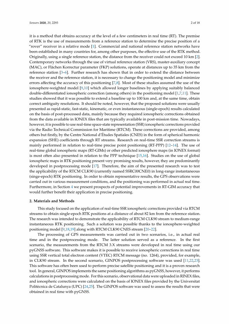
The pyGNSS software made it possible to use real-time SSR corrections, as well as data modelsstored, for example, in ANTEX and IONEX formats for phase center and ionospheric corrections,to augment performed estimations. The software operated according to the following scheme shownin Figure 1.
Sensors 2020, 20, 2293 3 of 18
main task was to perform satellite positioning in real time using RTCM 3.X streams. Single point
positioning (SPP), differential GPS (DGPS), and long-range instantaneous RTK positioning
algorithms were implemented. The software was also able to calculate longer observation sessions in
real time. Using the application was possible through Graphical User Interface (GUI) designed in
QT4 through pyQT4 bindings. Access to the intermediate and final results was possible almost at
any stage of processing.
The pyGNSS software made it possible to use real-time SSR corrections, as well as data models
stored, for example, in ANTEX and IONEX formats for phase center and ionospheric corrections, to
augment performed estimations. The software operated according to the following scheme shown in
Figure 1.
Figure 1. The data flow diagram of the pyGNSS software.
The purpose of the study was to process real-time kinematic medium-length baselines with
1-second measurement intervals using single-epoch GPS measurements. This approach is often
called instantaneous positioning, as each epoch of data is being processed. For this reason, the
ionosphere-weighted algorithm that uses double-differenced (DD) ionospheric delays as
pseudo-observations in the positioning model, was implemented. The functional model also used
double-differenced phase and code observables. The model is given as [26]:
𝜆1φ1,𝑖𝑗𝑘𝑙 − 𝜌𝑖𝑗
𝑘𝑙 − (𝛼𝑖𝑘𝑍𝑇𝐷𝑖 − 𝛼𝑖
𝑙𝑍𝑇𝐷𝑖 − 𝛼𝑗𝑘𝑍𝑇𝐷𝑗 + 𝛼𝑗
𝑙𝑍𝑇𝐷𝑗 ) + 𝐼𝑖𝑗𝑘𝑙 − 𝜆1𝑁1,𝑖𝑗
𝑘𝑙 = 0
𝜆2φ2,𝑖𝑗𝑘𝑙 − 𝜌𝑖𝑗
𝑘𝑙 − (𝛼𝑖𝑘𝑍𝑇𝐷𝑖 − 𝛼𝑖
𝑙𝑍𝑇𝐷𝑖 − 𝛼𝑗𝑘𝑍𝑇𝐷𝑗 + 𝛼𝑗
𝑙𝑍𝑇𝐷𝑗 ) + (𝑓12/𝑓2
2)𝐼𝑖𝑗𝑘𝑙 − 𝜆2𝑁2,𝑖𝑗
𝑘𝑙 = 0
P1,𝑖𝑗𝑘𝑙 − 𝜌𝑖𝑗
𝑘𝑙 − (𝛼𝑖𝑘𝑍𝑇𝐷𝑖 − 𝛼𝑖
𝑙𝑍𝑇𝐷𝑖 − 𝛼𝑗𝑘𝑍𝑇𝐷𝑗 + 𝛼𝑗
𝑙𝑍𝑇𝐷𝑗 ) − 𝐼𝑖𝑗𝑘𝑙 = 0
where i and j are the receiver indexes; k and l are the satellite indexes; 𝜌𝑖𝑗𝑘𝑙 is the DD geometric
range; φ𝑛,𝑖𝑗𝑘𝑙 is the DD carrier-phase observable on frequency n; P1,𝑖𝑗
𝑘𝑙 is the DD pseudo-range
observable; 𝐼𝑖𝑗𝑘𝑙 is the DD ionospheric delay; 𝑍𝑇𝐷𝑖 is the Zenith tropospheric delay; 𝛼𝑖 is the
troposphere mapping function; 𝑁𝑛,𝑖𝑗𝑘𝑙 is the carrier-phase ambiguities on frequency n; 𝑓1 and 𝑓2
are the GPS frequencies of the L1 and L2 signals; 𝜆1 and 𝜆2 are wavelengths of the L1 and L2
signals.
The model presented in the software requires dual-frequency carrier phase, and
single-frequency pseudorange GPS observations. The unknown parameters are as follows:
Figure 1. The data flow diagram of the pyGNSS software.
The purpose of the study was to process real-time kinematic medium-length baselineswith 1-second measurement intervals using single-epoch GPS measurements. This approachis often called instantaneous positioning, as each epoch of data is being processed. For thisreason, the ionosphere-weighted algorithm that uses double-differenced (DD) ionospheric delays aspseudo-observations in the positioning model, was implemented. The functional model also useddouble-differenced phase and code observables. The model is given as [26]:
λ1ϕkl1,i j − ρ
kli j −
(αk
i ZTDi − αliZTDi − α
kjZTD j + α
ljZTD j
)+ Ikl
i j − λ1Nkl1,i j = 0
λ2ϕkl2,i j − ρ
kli j −
(αk
i ZTDi − αliZTDi − α
kjZTD j + α
ljZTD j
)+
(f 21 / f 2
2
)Ikli j − λ2Nkl
2,i j = 0
Pkl1,i j − ρ
kli j −
(αk
i ZTDi − αliZTDi − α
kjZTD j + α
ljZTD j
)− Ikl
i j = 0
where i and j are the receiver indexes; k and l are the satellite indexes; ρkli j is the DD geometric range;ϕkl
n,i j
is the DD carrier-phase observable on frequency n; Pkl1,i j is the DD pseudo-range observable; Ikl
i j is theDD ionospheric delay; ZTDi is the Zenith tropospheric delay; αi is the troposphere mapping function;Nkl
n,i j is the carrier-phase ambiguities on frequency n; f1 and f2 are the GPS frequencies of the L1 andL2 signals; λ1 and λ2 are wavelengths of the L1 and L2 signals.
Sensors 2020, 20, 2293 4 of 18
The model presented in the software requires dual-frequency carrier phase, and single-frequencypseudorange GPS observations. The unknown parameters are as follows:
• User receiver coordinates;• Double-differenced (DD) ionospheric delays;• Zenith tropospheric delays;• Double-differenced (DD) integer ambiguities.
All the parameters are constrained to some a priori information, which can consist of empiricalvalues. In the case of ionospheric corrections, a priori values were calculated on the basis ofSHE coefficients provided in RTCM 3.X message 1264. For the calculation of tropospheric correction,the UNB3m model with Neil mapping function was selected to determine slant tropospheric correctionsthat were fixed in the processing [27–29].
To determine integer ambiguity values, a classic three-step solution was used as follows: A floatsolution with the ambiguities as real numbers in step one, an integer ambiguity search in second step,and a fixed solution in which real-valued ambiguities are replaced by the integers in step three [30,31].The least-squares ambiguity decorrelation adjustment (LAMBDA) was used to fix the ambiguities totheir integer values [32].
The most innovative feature introduced by the pyGNSS software is the use of SSR VTEC RTCMmessage (no. 1264) to obtain the ionospheric corrections in real time. VTEC, in this message,was provided using the SHE coefficients. The implementation was based on the following proposalof new RTCM SSR messages SSR Stage 2: VTEC for RTCM STANDARD 10403.2, differential GNSS,and services version 3 developed by RTCM special committee no. 104 [33]. According to this standard,the VTEC contribution is computed in TECU as:
VTEC(φPP,λPP) =N∑
n=0
min(n,M)∑m=0
(cnm cos(mλs) + snm sin(mλS))Pnm(sinφPP)
where N is the degree of spherical expansion (DF474), M is the order of spherical expansion (DF475),n and m are indexes, cnm is the cosine coefficient for the layer (DF476), snm is the sine coefficientfor the layer (DF477), λs is the mean sun fixed and phase shifted longitude of ionospheric piercepoint for the layer, λPP is the longitude of ionospheric pierce point for the layer, t is GPS time, ϕPP
is geocentric latitude of ionospheric pierce point for the layer, and Pnm( ) are the fully normalizedassociated Legendre functions.
3. Results
3.1. Experiment Description
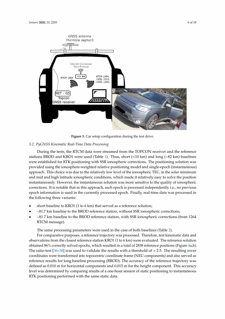
The experiment was carried out on 30 April 2019 (DOY 120) between 9:30 am. and 10:30 am.During the test, a car was equipped with a GPS receiver, Internet communication, and a computer torecord and process observational data. A Topcon NET-G5 receiver was used for this research. It is ahigh-class receiver primarily used for reference stations, so it was possible to save raw observation datain RINEX format, and also transfer RTCM streams using the NTRIP caster protocol at the same time.A Trimble zephyr 3 antenna was connected to the receiver. The Topcon receiver collected observationsat 1 Hz frequency, data were recorded in the RINEX format, and in parallel transmitted as RTCMstreams. The obtained GPS data were calculated in two scenarios:
• Real-time instantaneous RTK positioning based on RTCM streams using the pyGNSS software;• Postprocessed instantaneous RTK using RINEX and IONEX files and calculated with the GINPOS
software [23,24].
For the case of actual real-time positioning, during the tests, the receiver sent raw observation data(RTCM 1004) via the wireless Internet network to the computer running pyGNSS. At the same time,
Sensors 2020, 20, 2293 5 of 18
the computer received reference station data and the necessary SSR correction data from the remainingsources (Table 1). Note that we did not use any correction data from ground-based augmentationsystems, for example, EUPOS [34,35].
Table 1. RTCM streams recorded during the test drive.
Source RTCM Data
Topcon NET-G5 1004, GPS raw measurement
BROD (82 km) reference station 1004, GPS raw measurement1006, station coordinates
KRO1 (1–6 km) reference station 1004, GPS raw measurement1006, station coordinates
CLK90 1264, SSR VTEC RTCM messageIGC01 1058, SSR SV eph and clock corrections
RTCM3EPH 1019, GPS satellites ephemeries
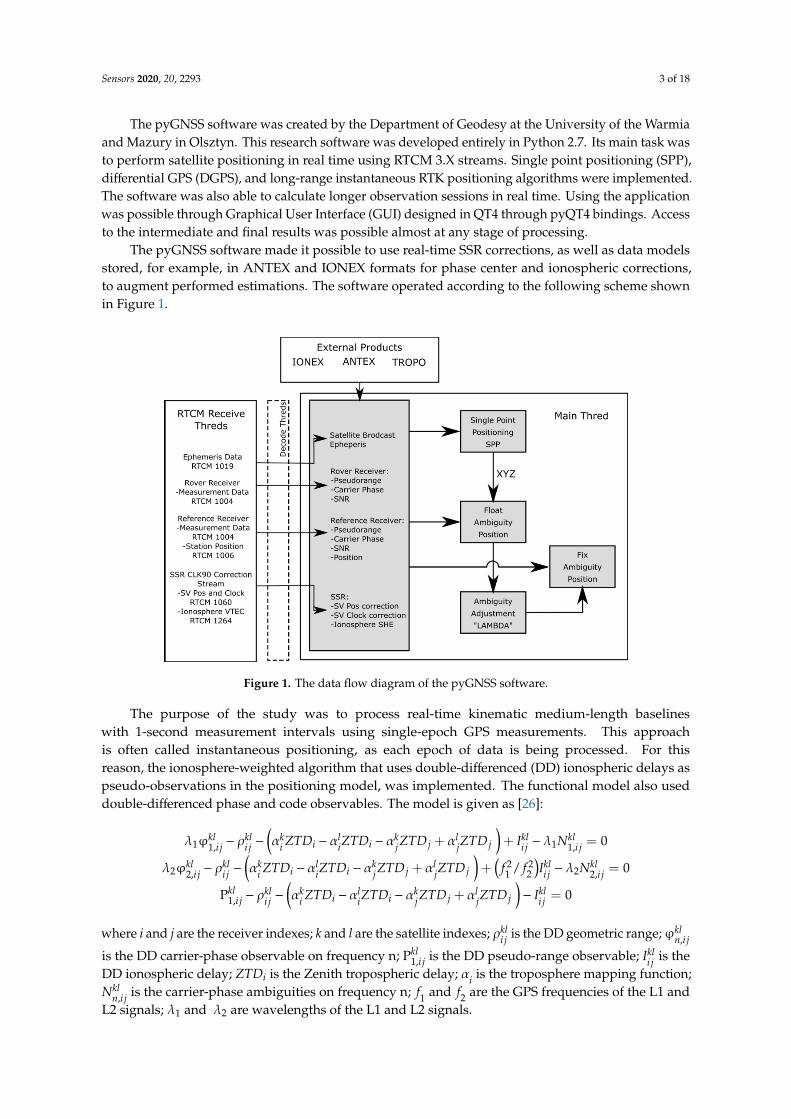
A car covered the route which was characterized by a variable exposure of the horizon. The testdrive lasted about 50 minutes, which provided the opportunity to collect 3300 measuring epochs.Figure 2 presents a Google Earth view of the entire route. The route was selected so that the carexperienced variable conditions. In the western and eastern parts, the car was driven through areaswith a clear horizon, whereas, in the south, the area was characterized by a higher urban development,and in the north by two-to three-storey buildings. The influence of covering the horizon by thebuildings is visible later on in the section describing the research results. The setup configuration ofthe car is presented in Figure 3.
Sensors 2020, 20, 2293 5 of 18
Table 1. RTCM streams recorded during the test drive.
Source RTCM Data
Topcon NET-G5 1004, GPS raw measurement
BROD (82 km) reference station 1004, GPS raw measurement
1006, station coordinates
KRO1 (1–6 km) reference station 1004, GPS raw measurement
1006, station coordinates
CLK90 1264, SSR VTEC RTCM message
IGC01 1058, SSR SV eph and clock corrections
RTCM3EPH 1019, GPS satellites ephemeries
A car covered the route which was characterized by a variable exposure of the horizon. The test
drive lasted about 50 minutes, which provided the opportunity to collect 3300 measuring epochs.
Figure 2 presents a Google Earth view of the entire route. The route was selected so that the car
experienced variable conditions. In the western and eastern parts, the car was driven through areas
with a clear horizon, whereas, in the south, the area was characterized by a higher urban
development, and in the north by two-to three-storey buildings. The influence of covering the
horizon by the buildings is visible later on in the section describing the research results. The setup
configuration of the car is presented in Figure 3.
Figure 2. Google Earth view of the car test route (Olsztyn, Poland).
Figure 2. Google Earth view of the car test route (Olsztyn, Poland).
Sensors 2020, 20, 2293 6 of 18Sensors 2020, 20, 2293 6 of 18
Figure 3. Car setup configuration during the test drive.
3.2. PyGNSS Kinematic Real-Time Data Processing
During the tests, the RTCM data were streamed from the TOPCON receiver and the reference
stations BROD and KRO1 were used (Table 1). Thus, short (<10 km) and long (~82 km) baselines
were established for RTK positioning with SSR ionospheric corrections. The positioning solution
was provided using the ionosphere-weighted relative positioning model and single-epoch
(instantaneous) approach. This choice was due to the relatively low level of the ionospheric TEC, in
the solar minimum and mid and high latitude ionospheric conditions, which made it relatively easy
to solve the position instantaneously. However, the instantaneous solution was more sensitive to the
quality of ionospheric corrections. It is notable that in this approach, each epoch is processed
independently, i.e., no previous epoch information is used in the currently processed epoch. Finally,
real-time data was processed in the following three variants:
short baseline to KRO1 (1 to 6 km) that served as a reference solution;
~81.7 km baseline to the BROD reference station, without SSR ionospheric corrections;
~81.7 km baseline to the BROD reference station, with SSR ionospheric corrections (from 1264
RTCM message).
The same processing parameters were used in the case of both baselines (Table 2).
Table 2. pyGNSS real-time processing parameters.
Parameter Value
GNSS system and signals GPS L1 and L2
Satellite orbits and clocks Broadcast + SSR correction
Positioning model relative, ionosphere and troposphere weighted
First data epoch 9:35 GPST
Last data epoch 10:30 GPST
Data interval 1 second
Session length 3300 epochs
Ambiguity resolution LAMBDA
Ambiguity selection validation Ratio-test
Figure 3. Car setup configuration during the test drive.
3.2. PyGNSS Kinematic Real-Time Data Processing
During the tests, the RTCM data were streamed from the TOPCON receiver and the referencestations BROD and KRO1 were used (Table 1). Thus, short (<10 km) and long (~82 km) baselineswere established for RTK positioning with SSR ionospheric corrections. The positioning solution wasprovided using the ionosphere-weighted relative positioning model and single-epoch (instantaneous)approach. This choice was due to the relatively low level of the ionospheric TEC, in the solar minimumand mid and high latitude ionospheric conditions, which made it relatively easy to solve the positioninstantaneously. However, the instantaneous solution was more sensitive to the quality of ionosphericcorrections. It is notable that in this approach, each epoch is processed independently, i.e., no previousepoch information is used in the currently processed epoch. Finally, real-time data was processed inthe following three variants:
• short baseline to KRO1 (1 to 6 km) that served as a reference solution;• ~81.7 km baseline to the BROD reference station, without SSR ionospheric corrections;• ~81.7 km baseline to the BROD reference station, with SSR ionospheric corrections (from 1264
RTCM message).
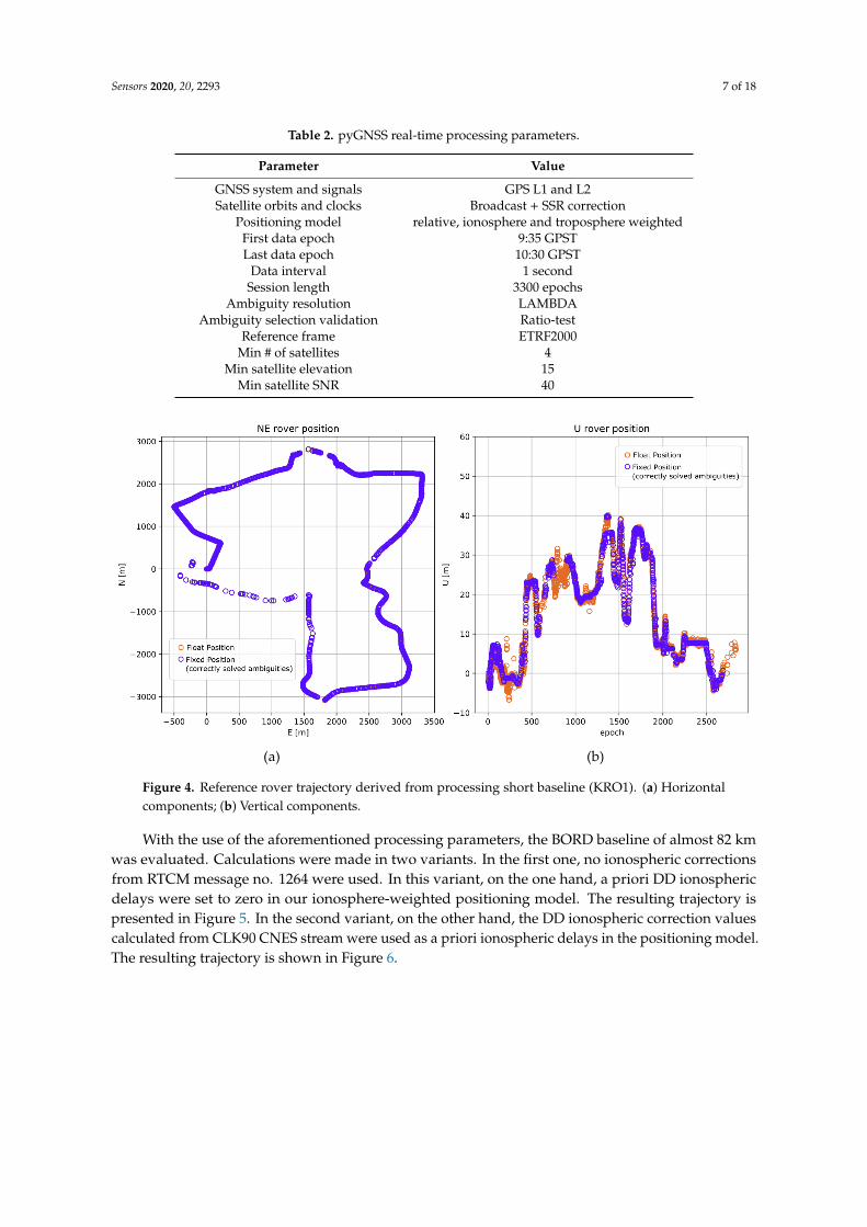
The same processing parameters were used in the case of both baselines (Table 2).For comparative purposes, a reference trajectory was processed. Therefore, test kinematic data and
observations from the closest reference station KRO1 (1 to 6 km) were evaluated. The reference solutionobtained 86% correctly solved epochs, which resulted in a total of 2838 reference positions (Figure 4a,b).The ratio-test [36–38] was used to validate the results with a threshold of > 2.5. The resulting rovercoordinates were transformed into topocentric coordinate frame (NEU components) and also served asreference results for long baseline processing (BROD). The accuracy of the reference trajectory wasdefined as 0.010 m for horizontal components and 0.015 m for the height component. This accuracylevel was determined by comparing results of a one-hour session of static positioning to instantaneousRTK positioning performed with the same static data.
Sensors 2020, 20, 2293 7 of 18
Table 2. pyGNSS real-time processing parameters.
Parameter Value
GNSS system and signals GPS L1 and L2Satellite orbits and clocks Broadcast + SSR correction
Positioning model relative, ionosphere and troposphere weightedFirst data epoch 9:35 GPSTLast data epoch 10:30 GPST
Data interval 1 secondSession length 3300 epochs
Ambiguity resolution LAMBDAAmbiguity selection validation Ratio-test
Reference frame ETRF2000Min # of satellites 4
Min satellite elevation 15Min satellite SNR 40
Sensors 2020, 20, 2293 7 of 18
Reference frame ETRF2000
Min # of satellites 4
Min satellite elevation 15
Min satellite SNR 40
For comparative purposes, a reference trajectory was processed. Therefore, test kinematic data
and observations from the closest reference station KRO1 (1 to 6 km) were evaluated. The reference
solution obtained 86% correctly solved epochs, which resulted in a total of 2838 reference positions
(Figure 4a,b). The ratio-test [36–38] was used to validate the results with a threshold of > 2.5. The
resulting rover coordinates were transformed into topocentric coordinate frame (NEU components)
and also served as reference results for long baseline processing (BROD). The accuracy of the
reference trajectory was defined as 0.010 m for horizontal components and 0.015 m for the height
component. This accuracy level was determined by comparing results of a one-hour session of static
positioning to instantaneous RTK positioning performed with the same static data.
(a) (b)
Figure 4. Reference rover trajectory derived from processing short baseline (KRO1). (a) Horizontal
components; (b) Vertical components.
With the use of the aforementioned processing parameters, the BORD baseline of almost 82 km
was evaluated. Calculations were made in two variants. In the first one, no ionospheric corrections
from RTCM message no. 1264 were used. In this variant, on the one hand, a priori DD ionospheric
delays were set to zero in our ionosphere-weighted positioning model. The resulting trajectory is
presented in Figure 5. In the second variant, on the other hand, the DD ionospheric correction values
calculated from CLK90 CNES stream were used as a priori ionospheric delays in the positioning
model. The resulting trajectory is shown in Figure 6.
Figure 4. Reference rover trajectory derived from processing short baseline (KRO1). (a) Horizontalcomponents; (b) Vertical components.
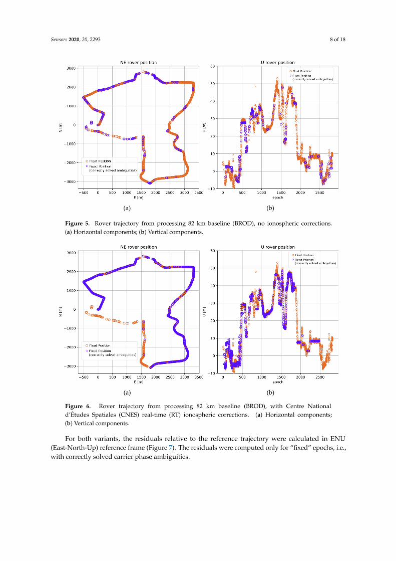
With the use of the aforementioned processing parameters, the BORD baseline of almost 82 kmwas evaluated. Calculations were made in two variants. In the first one, no ionospheric correctionsfrom RTCM message no. 1264 were used. In this variant, on the one hand, a priori DD ionosphericdelays were set to zero in our ionosphere-weighted positioning model. The resulting trajectory ispresented in Figure 5. In the second variant, on the other hand, the DD ionospheric correction valuescalculated from CLK90 CNES stream were used as a priori ionospheric delays in the positioning model.The resulting trajectory is shown in Figure 6.
Sensors 2020, 20, 2293 8 of 18Sensors 2020, 20, 2293 8 of 18
(a) (b)
Figure 5. Rover trajectory from processing 82 km baseline (BROD), no ionospheric corrections. (a)
Horizontal components; (b) Vertical components.
(a) (b)
Figure 6. Rover trajectory from processing 82 km baseline (BROD), with Centre National d'Études
Spatiales (CNES) real-time (RT) ionospheric corrections. (a) Horizontal components; (b) Vertical
components.
For both variants, the residuals relative to the reference trajectory were calculated in ENU
(East-North-Up) reference frame (Figure 7). The residuals were computed only for “fixed” epochs,
i.e., with correctly solved carrier phase ambiguities.
Figure 5. Rover trajectory from processing 82 km baseline (BROD), no ionospheric corrections.(a) Horizontal components; (b) Vertical components.
Sensors 2020, 20, 2293 8 of 18
(a) (b)
Figure 5. Rover trajectory from processing 82 km baseline (BROD), no ionospheric corrections. (a)
Horizontal components; (b) Vertical components.
(a) (b)
Figure 6. Rover trajectory from processing 82 km baseline (BROD), with Centre National d'Études
Spatiales (CNES) real-time (RT) ionospheric corrections. (a) Horizontal components; (b) Vertical
components.
For both variants, the residuals relative to the reference trajectory were calculated in ENU
(East-North-Up) reference frame (Figure 7). The residuals were computed only for “fixed” epochs,
i.e., with correctly solved carrier phase ambiguities.
Figure 6. Rover trajectory from processing 82 km baseline (BROD), with Centre Nationald’Études Spatiales (CNES) real-time (RT) ionospheric corrections. (a) Horizontal components;(b) Vertical components.
For both variants, the residuals relative to the reference trajectory were calculated in ENU(East-North-Up) reference frame (Figure 7). The residuals were computed only for “fixed” epochs, i.e.,with correctly solved carrier phase ambiguities.
Sensors 2020, 20, 2293 9 of 18Sensors 2020, 20, 2293 9 of 18
(a) (b)
Figure 7. Rover position residua vs. the reference solution from processing the BROD baseline.
(a) Without ionospheric corrections; (b) With CNES RT ionospheric corrections. Horizontal residua dE;
dN are shown in orange and red, respectively; and blue depicts height component.
Table 3 presents the statistics of the obtained results. The metrics used for statistical analysis of
the positioning results are ambiguity resolution success rate (ARSR) and ambiguity validation
failure ratio (AVRF). The ARSR presents the percentage of processed epochs with correctly fixed
ambiguities, while the AVRF is the percentage of epochs with the ratio-test higher than that of the
threshold (ratio-test > 2.5), but they were not correct (wrong ambiguity fixes). This was validated by
the comparisons with the reference solution from the processing of the short baseline. Therefore, the
ARSR_true parameter shows the externally validated success of the ambiguity resolution.
Table 3. Statistics of real-time solutions.
Ref. Station Baseline (km) ARSR (%) AVFR (%) ARSR_True (%) Iono Corr.
KRO1 1–6 km 86.22 - - no
BROD 81.7 19.34 15.68 16.31 no
BROD 81.7 58.66 5.03 55.71 yes
On the one hand, the trajectory obtained by processing the BROD baseline without the use of
ionospheric corrections is characterized by a very low ARSR_true (~17%) and high number of wrong
fixes (~16%). Only 538 epochs from the collected measurement set were solved correctly. On the
other hand, the use of ionospheric corrections in the model significantly improved the obtained
results. As can be observed in Table 3, the success rate of the ambiguity resolution increased from
~17% to ~56%, which was 1838 epochs, gaining a three-fold improvement in the success ratio. More
importantly, the AVRF parameter was reduced from ~15% to ~5%.
At the same time, in Figure 7, it can be noticed that the accuracy of the results obtained in both
variants is quite similar. Slightly higher residuals are observed for the second variant. Note,
however, that the solution with the CNES ionospheric corrections resulted in solving three times
more epochs, which mostly concerned cases with a lower number of satellites (higher PDOP). The
average values of the residuals’ oscillate were approximately 0.005 m and the standard deviations
did not exceed 0.025 m. On the basis of the obtained results, it can be stated that the application of
the RT CNES corrections, provided via RTCM stream for processing long-range kinematic solution,
and improved the success rate and reliability of positioning results while maintaining the same
accuracy.
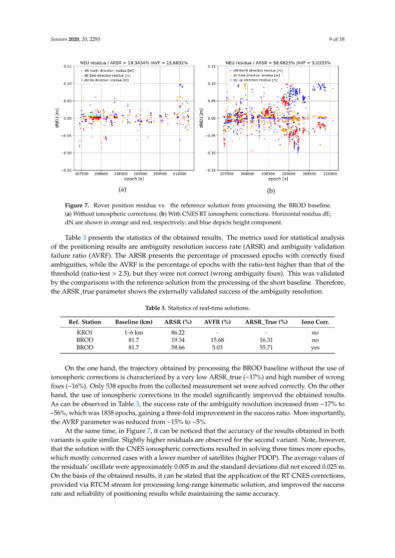
Figure 7. Rover position residua vs. the reference solution from processing the BROD baseline.(a) Without ionospheric corrections; (b) With CNES RT ionospheric corrections. Horizontal residua dE;dN are shown in orange and red, respectively; and blue depicts height component.
Table 3 presents the statistics of the obtained results. The metrics used for statistical analysisof the positioning results are ambiguity resolution success rate (ARSR) and ambiguity validationfailure ratio (AVRF). The ARSR presents the percentage of processed epochs with correctly fixedambiguities, while the AVRF is the percentage of epochs with the ratio-test higher than that of thethreshold (ratio-test > 2.5), but they were not correct (wrong ambiguity fixes). This was validatedby the comparisons with the reference solution from the processing of the short baseline. Therefore,the ARSR_true parameter shows the externally validated success of the ambiguity resolution.
Table 3. Statistics of real-time solutions.
Ref. Station Baseline (km) ARSR (%) AVFR (%) ARSR_True (%) Iono Corr.
KRO1 1–6 km 86.22 - - noBROD 81.7 19.34 15.68 16.31 noBROD 81.7 58.66 5.03 55.71 yes
On the one hand, the trajectory obtained by processing the BROD baseline without the use ofionospheric corrections is characterized by a very low ARSR_true (~17%) and high number of wrongfixes (~16%). Only 538 epochs from the collected measurement set were solved correctly. On the otherhand, the use of ionospheric corrections in the model significantly improved the obtained results.As can be observed in Table 3, the success rate of the ambiguity resolution increased from ~17% to~56%, which was 1838 epochs, gaining a three-fold improvement in the success ratio. More importantly,the AVRF parameter was reduced from ~15% to ~5%.
At the same time, in Figure 7, it can be noticed that the accuracy of the results obtained in bothvariants is quite similar. Slightly higher residuals are observed for the second variant. Note, however,that the solution with the CNES ionospheric corrections resulted in solving three times more epochs,which mostly concerned cases with a lower number of satellites (higher PDOP). The average values ofthe residuals’ oscillate were approximately 0.005 m and the standard deviations did not exceed 0.025 m.On the basis of the obtained results, it can be stated that the application of the RT CNES corrections,provided via RTCM stream for processing long-range kinematic solution, and improved the successrate and reliability of positioning results while maintaining the same accuracy.
Sensors 2020, 20, 2293 10 of 18
3.3. GINPOS: Kinematic Data Processed in Postprocessing
Additionally, independent tests were carried out in the postprocessing mode using UWM GINPOSsoftware developed in Matlab [39–41]. These tests were performed in order to provide another referencefor the results obtained in real time. In this scenario, three reference stations were selected which resultedin the formation of short (<10 km), medium (~60 km), and long (~82 km) baselines. The solution wasprovided using the ionosphere-weighted relative positioning model with a single-epoch (instantaneous)approach, as was in the case of real-time scenario. The kinematic data described in Section 3.1 wereprocessed in several variants as follows:
• A short baseline (1 to 6 km) that served as a reference solution;• a 62 km baseline to the DZIA reference station, with and without ionospheric corrections;• an 81.7 km baseline to the BROD reference station, with and without ionospheric corrections;• multi-baseline (61, 62, and 81.7 km to MRAG, DZIA, and BROD), with and without
ionospheric corrections.
In the case of all baselines, the same processing parameters were used (Table 4). In thepostprocessing tests, however, the ionospheric corrections were derived from UQRG GIMs computedby UPC-IonSAT [25,26,42].
Table 4. Processing parameters.
Parameter Value
GNSS system and signals GPS L1 and L2Satellite orbits and clocks Int. GNSS Service (IGS) ultrarapid (predicted part)
Positioning model relative, ionosphere and troposphere weightedFirst data epoch 9:35 GPSTLast data epoch 10:30 GPST
Data interval 1 secondSession length 3300 epochs
Ambiguity resolution LAMBDAAmbiguity selection validation W-test
Reference frame ETRF2000PDOP threshold 7W-test threshold 3Min # of satellites 4
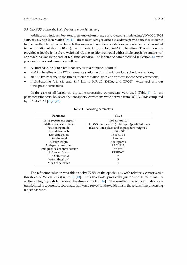
The reference solution was able to solve 77.5% of the epochs, i.e., with relatively conservativethreshold of W-test > 3 (Figure 8) [43]. This threshold practically guaranteed 100% reliabilityof the ambiguity validation over baselines < 10 km [44]. The resulting rover coordinates weretransformed to topocentric coordinate frame and served for the validation of the results from processinglonger baselines.
Sensors 2020, 20, 2293 11 of 18Sensors 2020, 20, 2293 11 of 18
(a) (b)
Figure 8. Reference rover trajectory derived from processing short baseline (KRO1). (a) Horizontal
components; (b) Vertical components.
Subsequent determinations were made for the DZIA reference station. The DZIA solution was
able to solve 35.6% of the epochs in the scenario without ionospheric correction, and 47.8% of the
epochs in the variant with the ionospheric corrections. This study shows that for a 62 km baseline,
12.2% more epochs were correctly resolved with the use of ionospheric corrections. The results are
shown in Figure 9. As for the reliability of the solution, in the first variant we obtained 0.87% wrong
fixes and only 0.41% in the second variant.
(a) (b)
Figure 9. Rover trajectory from processing 62 km baseline (DZIA). (a) No ionospheric corrections;
(b) With ionospheric corrections.
Figure 10 shows the residual values relative to a reference trajectory. As in the real-time
scenario, the coordinates in the ENU coordinate frame were compared.
Figure 8. Reference rover trajectory derived from processing short baseline (KRO1). (a) Horizontalcomponents; (b) Vertical components.
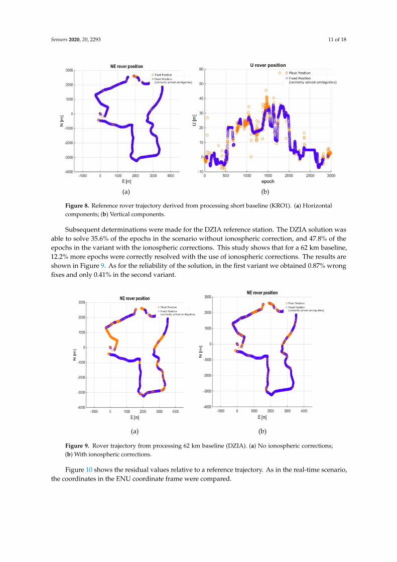
Subsequent determinations were made for the DZIA reference station. The DZIA solution wasable to solve 35.6% of the epochs in the scenario without ionospheric correction, and 47.8% of theepochs in the variant with the ionospheric corrections. This study shows that for a 62 km baseline,12.2% more epochs were correctly resolved with the use of ionospheric corrections. The results areshown in Figure 9. As for the reliability of the solution, in the first variant we obtained 0.87% wrongfixes and only 0.41% in the second variant.
Sensors 2020, 20, 2293 11 of 18
(a) (b)
Figure 8. Reference rover trajectory derived from processing short baseline (KRO1). (a) Horizontal
components; (b) Vertical components.
Subsequent determinations were made for the DZIA reference station. The DZIA solution was
able to solve 35.6% of the epochs in the scenario without ionospheric correction, and 47.8% of the
epochs in the variant with the ionospheric corrections. This study shows that for a 62 km baseline,
12.2% more epochs were correctly resolved with the use of ionospheric corrections. The results are
shown in Figure 9. As for the reliability of the solution, in the first variant we obtained 0.87% wrong
fixes and only 0.41% in the second variant.
(a) (b)
Figure 9. Rover trajectory from processing 62 km baseline (DZIA). (a) No ionospheric corrections;
(b) With ionospheric corrections.
Figure 10 shows the residual values relative to a reference trajectory. As in the real-time
scenario, the coordinates in the ENU coordinate frame were compared.
Figure 9. Rover trajectory from processing 62 km baseline (DZIA). (a) No ionospheric corrections;(b) With ionospheric corrections.
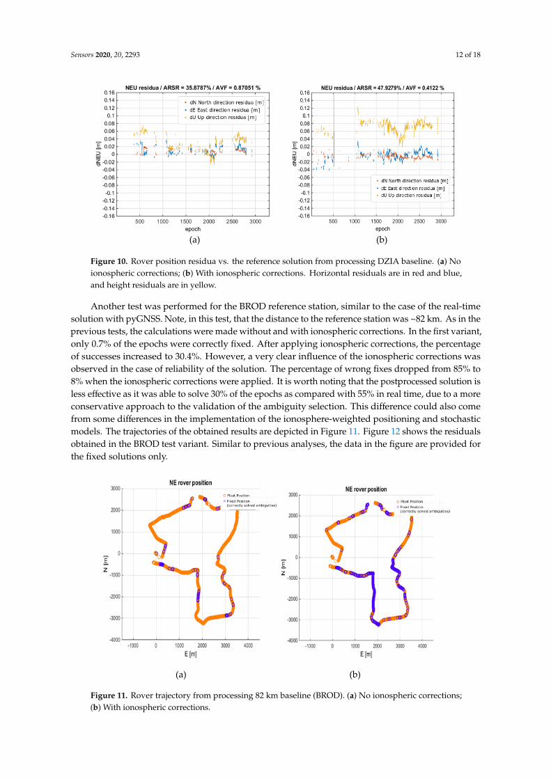
Figure 10 shows the residual values relative to a reference trajectory. As in the real-time scenario,the coordinates in the ENU coordinate frame were compared.
Sensors 2020, 20, 2293 12 of 18
Sensors 2020, 20, 2293 12 of 18
(a) (b)
Figure 10. Rover position residua vs. the reference solution from processing DZIA baseline. (a) No
ionospheric corrections; (b) With ionospheric corrections. Horizontal residuals are in red and blue,
and height residuals are in yellow.
Another test was performed for the BROD reference station, similar to the case of the real-time
solution with pyGNSS. Note, in this test, that the distance to the reference station was ~82 km. As in
the previous tests, the calculations were made without and with ionospheric corrections. In the first
variant, only 0.7% of the epochs were correctly fixed. After applying ionospheric corrections, the
percentage of successes increased to 30.4%. However, a very clear influence of the ionospheric
corrections was observed in the case of reliability of the solution. The percentage of wrong fixes
dropped from 85% to 8% when the ionospheric corrections were applied. It is worth noting that the
postprocessed solution is less effective as it was able to solve 30% of the epochs as compared with
55% in real time, due to a more conservative approach to the validation of the ambiguity selection.
This difference could also come from some differences in the implementation of the
ionosphere-weighted positioning and stochastic models. The trajectories of the obtained results are
depicted in Figure 11. Figure 12 shows the residuals obtained in the BROD test variant. Similar to
previous analyses, the data in the figure are provided for the fixed solutions only.
(a) (b)
Figure 11. Rover trajectory from processing 82 km baseline (BROD). (a) No ionospheric corrections;
(b) With ionospheric corrections.
Figure 10. Rover position residua vs. the reference solution from processing DZIA baseline. (a) Noionospheric corrections; (b) With ionospheric corrections. Horizontal residuals are in red and blue,and height residuals are in yellow.
Another test was performed for the BROD reference station, similar to the case of the real-timesolution with pyGNSS. Note, in this test, that the distance to the reference station was ~82 km. As in theprevious tests, the calculations were made without and with ionospheric corrections. In the first variant,only 0.7% of the epochs were correctly fixed. After applying ionospheric corrections, the percentageof successes increased to 30.4%. However, a very clear influence of the ionospheric corrections wasobserved in the case of reliability of the solution. The percentage of wrong fixes dropped from 85% to8% when the ionospheric corrections were applied. It is worth noting that the postprocessed solution isless effective as it was able to solve 30% of the epochs as compared with 55% in real time, due to a moreconservative approach to the validation of the ambiguity selection. This difference could also comefrom some differences in the implementation of the ionosphere-weighted positioning and stochasticmodels. The trajectories of the obtained results are depicted in Figure 11. Figure 12 shows the residualsobtained in the BROD test variant. Similar to previous analyses, the data in the figure are provided forthe fixed solutions only.
Sensors 2020, 20, 2293 12 of 18
(a) (b)
Figure 10. Rover position residua vs. the reference solution from processing DZIA baseline. (a) No
ionospheric corrections; (b) With ionospheric corrections. Horizontal residuals are in red and blue,
and height residuals are in yellow.
Another test was performed for the BROD reference station, similar to the case of the real-time
solution with pyGNSS. Note, in this test, that the distance to the reference station was ~82 km. As in
the previous tests, the calculations were made without and with ionospheric corrections. In the first
variant, only 0.7% of the epochs were correctly fixed. After applying ionospheric corrections, the
percentage of successes increased to 30.4%. However, a very clear influence of the ionospheric
corrections was observed in the case of reliability of the solution. The percentage of wrong fixes
dropped from 85% to 8% when the ionospheric corrections were applied. It is worth noting that the
postprocessed solution is less effective as it was able to solve 30% of the epochs as compared with
55% in real time, due to a more conservative approach to the validation of the ambiguity selection.
This difference could also come from some differences in the implementation of the
ionosphere-weighted positioning and stochastic models. The trajectories of the obtained results are
depicted in Figure 11. Figure 12 shows the residuals obtained in the BROD test variant. Similar to
previous analyses, the data in the figure are provided for the fixed solutions only.
(a) (b)
Figure 11. Rover trajectory from processing 82 km baseline (BROD). (a) No ionospheric corrections;
(b) With ionospheric corrections.
Figure 11. Rover trajectory from processing 82 km baseline (BROD). (a) No ionospheric corrections;(b) With ionospheric corrections.
Sensors 2020, 20, 2293 13 of 18Sensors 2020, 20, 2293 13 of 18
(a) (b)
Figure 12. Rover position residua vs. the reference position from processing BROD baseline. (a) No
ionospheric corrections; (b) With ionospheric corrections. Horizontal residuals are in red and blue,
and height residuals are in yellow.
The GINPOS software, however, was able to process a multi-baseline solution, i.e., when the
data from several reference stations are adjusted in a single positioning model [11,27,45,46]. This
strengthens the positioning model. Therefore, the last variant concerned the multi-baseline
positioning using MRAG, DZIA, and BROD reference stations (denoted MULTI3). Their lengths
ranged from 62 to 82 km. As expected, the results were clearly improved. The use of the
multi-baseline solution resulted in a 62% success rate without ionospheric corrections and 72% with
the application of corrections. More importantly, the reliability of the solution for both variants is
high, i.e., the AVFR for the solution without and with ionospheric corrections dropped to 0.13% and
0.11%, respectively. The obtained trajectories are shown in Figure 13 and the residual analysis
against reference solution is presented in Figure 14. Residua of the horizontal components of the
fixed solution are within +/- 3 cm from the reference solution. In the case of the vertical component,
the residuals are up to + 6 cm.
(a) (b)
Figure 13. Rover trajectory from processing 62 to 82 km baselines (MULTI3). (a) No ionospheric
corrections; (b) With ionospheric corrections.
Figure 12. Rover position residua vs. the reference position from processing BROD baseline. (a) Noionospheric corrections; (b) With ionospheric corrections. Horizontal residuals are in red and blue,and height residuals are in yellow.
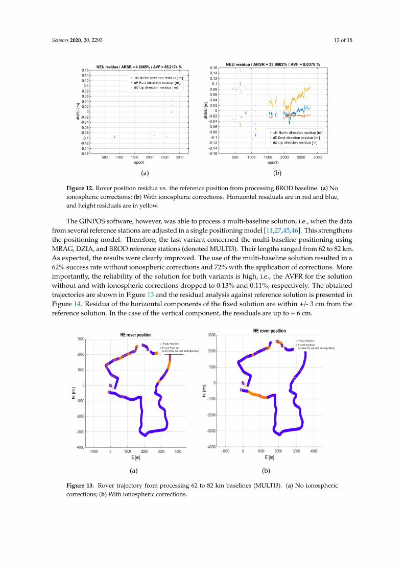
The GINPOS software, however, was able to process a multi-baseline solution, i.e., when the datafrom several reference stations are adjusted in a single positioning model [11,27,45,46]. This strengthensthe positioning model. Therefore, the last variant concerned the multi-baseline positioning usingMRAG, DZIA, and BROD reference stations (denoted MULTI3). Their lengths ranged from 62 to 82 km.As expected, the results were clearly improved. The use of the multi-baseline solution resulted in a62% success rate without ionospheric corrections and 72% with the application of corrections. Moreimportantly, the reliability of the solution for both variants is high, i.e., the AVFR for the solutionwithout and with ionospheric corrections dropped to 0.13% and 0.11%, respectively. The obtainedtrajectories are shown in Figure 13 and the residual analysis against reference solution is presented inFigure 14. Residua of the horizontal components of the fixed solution are within +/- 3 cm from thereference solution. In the case of the vertical component, the residuals are up to + 6 cm.
Sensors 2020, 20, 2293 13 of 18
(a) (b)
Figure 12. Rover position residua vs. the reference position from processing BROD baseline. (a) No
ionospheric corrections; (b) With ionospheric corrections. Horizontal residuals are in red and blue,
and height residuals are in yellow.
The GINPOS software, however, was able to process a multi-baseline solution, i.e., when the
data from several reference stations are adjusted in a single positioning model [11,27,45,46]. This
strengthens the positioning model. Therefore, the last variant concerned the multi-baseline
positioning using MRAG, DZIA, and BROD reference stations (denoted MULTI3). Their lengths
ranged from 62 to 82 km. As expected, the results were clearly improved. The use of the
multi-baseline solution resulted in a 62% success rate without ionospheric corrections and 72% with
the application of corrections. More importantly, the reliability of the solution for both variants is
high, i.e., the AVFR for the solution without and with ionospheric corrections dropped to 0.13% and
0.11%, respectively. The obtained trajectories are shown in Figure 13 and the residual analysis
against reference solution is presented in Figure 14. Residua of the horizontal components of the
fixed solution are within +/- 3 cm from the reference solution. In the case of the vertical component,
the residuals are up to + 6 cm.
(a) (b)
Figure 13. Rover trajectory from processing 62 to 82 km baselines (MULTI3). (a) No ionospheric
corrections; (b) With ionospheric corrections.
Figure 13. Rover trajectory from processing 62 to 82 km baselines (MULTI3). (a) No ionosphericcorrections; (b) With ionospheric corrections.
Sensors 2020, 20, 2293 14 of 18Sensors 2020, 20, 2293 14 of 18
(a) (b)
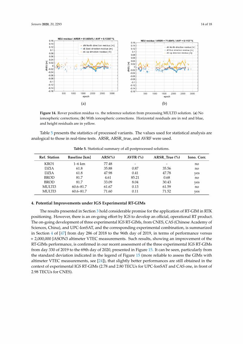
Figure 14. Rover position residua vs. the reference solution from processing MULTI3 solution. (a) No
ionospheric corrections; (b) With ionospheric corrections. Horizontal residuals are in red and blue,
and height residuals are in yellow.
Table 5 presents the statistics of processed variants. The values used for statistical analysis are
analogical to those in real-time tests. ARSR, ARSR_true, and AVRF were used.
Table 5. Statistical summary of all postprocessed solutions.
Ref. Station Baseline [km] ARS(%) AVFR (%) ARSR_True (%) Iono. Corr.
KRO1 1–6 km 77.48 - - no
DZIA 61.8 35.88 0.87 35.56 no
DZIA 61.8 47.98 0.41 47.78 yes
BROD 81.7 4.61 85.21 0.68 no
BROD 81.7 33.09 8.04 30.43 yes
MULTI3 60.6–81.7 61.67 0.13 61.59 no
MULTI3 60.6–81.7 71.60 0.11 71.52 yes
4. Potential Improvements under IGS Experimental RT-GIMs
The results presented in Section 3 hold considerable promise for the application of RT-GIM in
RTK positioning. However, there is an on-going effort by IGS to develop an official, operational RT
product. The on-going development of three experimental IGS RT-GIMs, from CNES, CAS (Chinese
Academy of Sciences, China), and UPC-IonSAT, and the corresponding experimental combination,
is summarized in Section 4 of [47] from day 286 of 2018 to the 96th day of 2019, in terms of
performance versus + 2,000,000 JASON3 altimeter VTEC measurements. Such results, showing an
improvement of the RT-GIMs performance, is confirmed in our recent assessment of the three
experimental IGS RT-GIMs from day 330 of 2019 to the 69th day of 2020, presented in Figure 15. It
can be seen, particularly from the standard deviation indicated in the legend of Figure 15 (more
reliable to assess the GIMs with altimeter VTEC measurements, see [24]), that slightly better
performances are still obtained in the context of experimental IGS RT-GIMs (2.78 and 2.80 TECUs for
UPC-IonSAT and CAS one, in front of 2.98 TECUs for CNES).
Figure 14. Rover position residua vs. the reference solution from processing MULTI3 solution. (a) Noionospheric corrections; (b) With ionospheric corrections. Horizontal residuals are in red and blue,and height residuals are in yellow.
Table 5 presents the statistics of processed variants. The values used for statistical analysis areanalogical to those in real-time tests. ARSR, ARSR_true, and AVRF were used.
Table 5. Statistical summary of all postprocessed solutions.
Ref. Station Baseline [km] ARS(%) AVFR (%) ARSR_True (%) Iono. Corr.
KRO1 1–6 km 77.48 - - noDZIA 61.8 35.88 0.87 35.56 noDZIA 61.8 47.98 0.41 47.78 yesBROD 81.7 4.61 85.21 0.68 noBROD 81.7 33.09 8.04 30.43 yes
MULTI3 60.6–81.7 61.67 0.13 61.59 noMULTI3 60.6–81.7 71.60 0.11 71.52 yes
4. Potential Improvements under IGS Experimental RT-GIMs
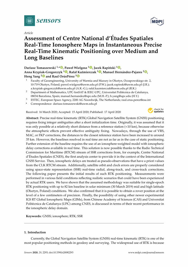
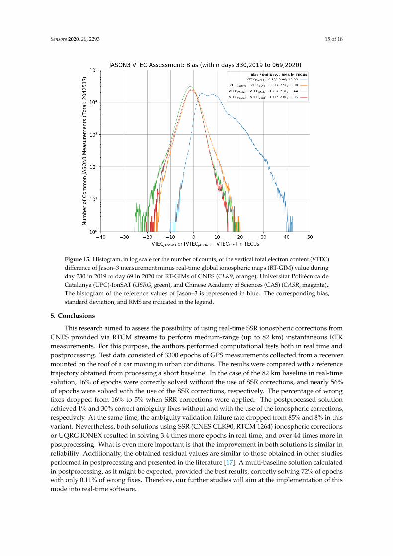
The results presented in Section 3 hold considerable promise for the application of RT-GIM in RTKpositioning. However, there is an on-going effort by IGS to develop an official, operational RT product.The on-going development of three experimental IGS RT-GIMs, from CNES, CAS (Chinese Academy ofSciences, China), and UPC-IonSAT, and the corresponding experimental combination, is summarizedin Section 4 of [47] from day 286 of 2018 to the 96th day of 2019, in terms of performance versus+ 2,000,000 JASON3 altimeter VTEC measurements. Such results, showing an improvement of theRT-GIMs performance, is confirmed in our recent assessment of the three experimental IGS RT-GIMsfrom day 330 of 2019 to the 69th day of 2020, presented in Figure 15. It can be seen, particularly fromthe standard deviation indicated in the legend of Figure 15 (more reliable to assess the GIMs withaltimeter VTEC measurements, see [24]), that slightly better performances are still obtained in thecontext of experimental IGS RT-GIMs (2.78 and 2.80 TECUs for UPC-IonSAT and CAS one, in front of2.98 TECUs for CNES).
Sensors 2020, 20, 2293 15 of 18Sensors 2020, 20, 2293 15 of 18
Figure 15. Histogram, in log scale for the number of counts, of the vertical total electron content
(VTEC) difference of Jason–3 measurement minus real-time global ionospheric maps (RT-GIM) value
during day 330 in 2019 to day 69 in 2020 for RT-GIMs of CNES (CLK9, orange), Universitat
Politècnica de Catalunya (UPC)-IonSAT (USRG, green), and Chinese Academy of Sciences (CAS)
(CASR, magenta),. The histogram of the reference values of Jason–3 is represented in blue. The
corresponding bias, standard deviation, and RMS are indicated in the legend.
5. Conclusions
This research aimed to assess the possibility of using real-time SSR ionospheric corrections from
CNES provided via RTCM streams to perform medium-range (up to 82 km) instantaneous RTK
measurements. For this purpose, the authors performed computational tests both in real time and
postprocessing. Test data consisted of 3300 epochs of GPS measurements collected from a receiver
mounted on the roof of a car moving in urban conditions. The results were compared with a
reference trajectory obtained from processing a short baseline. In the case of the 82 km baseline in
real-time solution, 16% of epochs were correctly solved without the use of SSR corrections, and
nearly 56% of epochs were solved with the use of the SSR corrections, respectively. The percentage
of wrong fixes dropped from 16% to 5% when SRR corrections were applied. The postprocessed
solution achieved 1% and 30% correct ambiguity fixes without and with the use of the ionospheric
corrections, respectively. At the same time, the ambiguity validation failure rate dropped from 85%
and 8% in this variant. Nevertheless, both solutions using SSR (CNES CLK90, RTCM 1264)
ionospheric corrections or UQRG IONEX resulted in solving 3.4 times more epochs in real time, and
over 44 times more in postprocessing. What is even more important is that the improvement in both
solutions is similar in reliability. Additionally, the obtained residual values are similar to those
obtained in other studies performed in postprocessing and presented in the literature [17]. A
multi-baseline solution calculated in postprocessing, as it might be expected, provided the best
results, correctly solving 72% of epochs with only 0.11% of wrong fixes. Therefore, our further
studies will aim at the implementation of this mode into real-time software.
Our initial results indicate that the use of corrections calculated on the basis of spherical
harmonics provided in the RTCM 1264 message significantly increases the success rate and
reliability of the instantaneous precise positioning. A further improvement in the results is expected
Figure 15. Histogram, in log scale for the number of counts, of the vertical total electron content (VTEC)difference of Jason–3 measurement minus real-time global ionospheric maps (RT-GIM) value duringday 330 in 2019 to day 69 in 2020 for RT-GIMs of CNES (CLK9, orange), Universitat Politècnica deCatalunya (UPC)-IonSAT (USRG, green), and Chinese Academy of Sciences (CAS) (CASR, magenta),.The histogram of the reference values of Jason–3 is represented in blue. The corresponding bias,standard deviation, and RMS are indicated in the legend.
5. Conclusions
This research aimed to assess the possibility of using real-time SSR ionospheric corrections fromCNES provided via RTCM streams to perform medium-range (up to 82 km) instantaneous RTKmeasurements. For this purpose, the authors performed computational tests both in real time andpostprocessing. Test data consisted of 3300 epochs of GPS measurements collected from a receivermounted on the roof of a car moving in urban conditions. The results were compared with a referencetrajectory obtained from processing a short baseline. In the case of the 82 km baseline in real-timesolution, 16% of epochs were correctly solved without the use of SSR corrections, and nearly 56%of epochs were solved with the use of the SSR corrections, respectively. The percentage of wrongfixes dropped from 16% to 5% when SRR corrections were applied. The postprocessed solutionachieved 1% and 30% correct ambiguity fixes without and with the use of the ionospheric corrections,respectively. At the same time, the ambiguity validation failure rate dropped from 85% and 8% in thisvariant. Nevertheless, both solutions using SSR (CNES CLK90, RTCM 1264) ionospheric correctionsor UQRG IONEX resulted in solving 3.4 times more epochs in real time, and over 44 times more inpostprocessing. What is even more important is that the improvement in both solutions is similar inreliability. Additionally, the obtained residual values are similar to those obtained in other studiesperformed in postprocessing and presented in the literature [17]. A multi-baseline solution calculatedin postprocessing, as it might be expected, provided the best results, correctly solving 72% of epochswith only 0.11% of wrong fixes. Therefore, our further studies will aim at the implementation of thismode into real-time software.
Sensors 2020, 20, 2293 16 of 18
Our initial results indicate that the use of corrections calculated on the basis of spherical harmonicsprovided in the RTCM 1264 message significantly increases the success rate and reliability of theinstantaneous precise positioning. A further improvement in the results is expected when theInternational GNSS Service starts its operational real-time ionospheric product. In particular, it hasbeen shown that other experimental IGS RT-GIMs, from CAS and UPC-IonSAT, have recently behavedsimilarly or slightly better than CNES, opening the way for a potentially better IGS-combined RT-GIM.In addition, real-time multi-station solutions shall clearly increase the success rate of the ambiguityfixing, bringing closer the operational application of the instantaneous RTK over longer baselines.
Author Contributions: Conceptualization, P.W. and D.T.; methodology, P.W.; software, D.T., J.R., and P.W.;validation, M.H.-P., A.K.-G., R.K., and H.Y.; formal analysis, P.W., and D.T.; investigation, J.R.; resources, P.W.and J.R.; data curation, M.H.-P., A.K.-G., R.K., and H.Y.; writing—original draft preparation, P.W. and D.T.;writing—review and editing, P.W.; visualization, P.W. and D.T.; supervision, J.R. and R.O.; project administration,A.K.-G. and R.O.; funding acquisition, P.W. and A.K.-G. All authors have read and agreed to the published versionof the manuscript.
Funding: This study was supported by ESA contract no. 4000119662/17/NL/CBi.
Acknowledgments: The authors are grateful to the Leica company and CODE, CNES, and IGS institutions forproviding data for research.
Conflicts of Interest: The authors declare no conflict of interest.
References
1. Langley, R.B. Rtk gps. Gps World 1998, 9, 70–76.2. Rizos, C.; Han, S. Reference station network based RTK systems-concepts and progress. Wuhan Univ. J. Nat.
Sci. 2003, 8, 566–574. [CrossRef]3. Hu, G.; Khoo, H.; Goh, P.; Law, C. Development and assessment of GPS virtual reference stations for RTK
positioning. J. Geod. 2003, 77, 292–302. [CrossRef]4. Hu, G.R.; Khoo, V.H.S.; Goh, P.C.; Law, C.L. Internet-based GPS VRS RTK positioning with a multiple
reference station network. Positioning 2009, 1, 114–120. [CrossRef]5. Vollath, U.; Landau, H.; Chen, X.; Doucet, K.; Pagels, C. Network RTK versus single base RTK–understanding
the error characteristics. In Proceedings of the 15th International Technical Meeting of the Satellite Divisionof the Institute of Navigation, Portland, OR, USA, 24–27 September 2002; pp. 24–27.
6. Vollath, U.; Deking, A.; Landau, H.; Pagels, C. Long-range RTK positioning using virtual reference stations.In Proceedings of the International Symposium on Kinematics Systems in Geodesy, Geomatics and Navication,Banff, AB, Canada, 5–8 June 2001.
7. Kim, D.; Langley, R.B. Long-range single-baseline RTK for complementing network-based RTK. Proc. IONGNSS 2007, 639–650.
8. Dai, L.; Eslinger, D.; Sharpe, T. Innovative algorithms to improve long range RTK reliability and availability.In Proceedings of the ION NTM, San Diego, CA, USA, 22–24 January 2007; pp. 860–872.
9. Odijk, D. Weighting ionospheric corrections to improve fast GPS positioning over medium distances.In Proceedings of the ION GPS, Salt Lake City, UT, USA, 19–22 September 2000; pp. 1113–1123.
10. Liu, G.C.; Lachapelle, G. Ionosphere weighted GPS cycle ambiguity resolution. In Proceedings of theProceedings of ION NTM, San Diego, CA, USA, 28–30 January 2002; pp. 889–899.
11. Wielgosz, P.; Kashani, I.; Grejner-Brzezinska, D. Analysis of long-range network RTK during a severeionospheric storm. J. Geod. 2005, 79, 524–531. [CrossRef]
12. Martín, A.; Anquela, A.; Dimas-Pagés, A.; Cos-Gayón, F. Validation of performance of real-time kinematicPPP. A possible tool for deformation monitoring. Measurement 2015, 69, 95–108. [CrossRef]
13. Gao, Y.; Zhang, W.; Li, Y. A new method for real-time PPP correction updates. In Proceedings of theInternational Symposium on Earth and Environmental Sciences for Future Generations, Prague, CzechRepublic, 22 June–2 July 2016; pp. 223–228.
14. Wang, Z.; Li, Z.; Wang, L.; Wang, X.; Yuan, H. Assessment of multiple GNSS real-time SSR products fromdifferent analysis centers. ISPRS Int. J. Geo-Inf. 2018, 7, 85. [CrossRef]
15. Ren, X.; Chen, J.; Li, X.; Zhang, X.; Freeshah, M. Performance evaluation of real-time global ionospheric mapsprovided by different IGS analysis centers. GPS Solut. 2019, 23, 113. [CrossRef]

Sensors 2020, 20, 2293 17 of 18
16. Ghoddousi-Fard, R.; Lahaye, F. Evaluation of single frequency GPS precise point positioning assisted withexternal ionosphere sources. Adv. Space Res. 2016, 57, 2154–2166. [CrossRef]
17. Grejner-Brzezinska, D.A.; Wielgosz, P.; Kashani, I.; Smith, D.A.; Robertson, D.S.; Mader, G.L.; Komjathy, A.The impact of severe ionospheric conditions on the accuracy of kinematic position estimation: Performanceanalysis of various ionosphere modeling techniques. Navigation 2006, 53, 203–217. [CrossRef]
18. Wielgosz, P. Quality assessment of GPS rapid static positioning with weighted ionospheric parameters ingeneralized least squares. Gps Solut. 2011, 15, 89–99. [CrossRef]
19. Teunissen, P. The ionosphere-weighted GPS baseline precision in canonical form. J. Geod. 1998, 72, 107–111.[CrossRef]
20. Nie, Z.; Yang, H.; Zhou, P.; Gao, Y.; Wang, Z. Quality assessment of CNES real-time ionospheric products.Gps Solut. 2019, 23, 11. [CrossRef]
21. Rülke, A.; Agrotis, L.; Enderle, W.; MacLeod, K. IGS real time service–status, future tasks and limitations.In Proceedings of the IGS Workshop; Federal Agency for Cartography and Geodesy: Frankfurt, Germany, 2016.
22. Wielgosz, P.; Paziewski, J.; Krankowski, A.; Kroszczynski, K.; Figurski, M. Results of the application oftropospheric corrections from different troposphere models for precise GPS rapid static positioning. ActaGeophys. 2012, 60, 1236–1257. [CrossRef]
23. Paziewski, J.; Stepniak, K.; Wielgosz, P.; Krypiak-Gregorczyk, A.; Krukowska, M. Multi-GNSS precisesingle-epoch positioning. Proc. EGU General Assem. Conf. Abstr. 2012, 14, 3561.
24. Hernández-Pajares, M.; Roma-Dollase, D.; Krankowski, A.; García-Rigo, A.; Orús-Pérez, R. Methodologyand consistency of slant and vertical assessments for ionospheric electron content models. J. Geod. 2017, 91,1405–1414. [CrossRef]
25. Roma-Dollase, D.; Hernández-Pajares, M.; Krankowski, A.; Kotulak, K.; Ghoddousi-Fard, R.; Yuan, Y.;Li, Z.; Zhang, H.; Shi, C.; Wang, C.; et al. Consistency of seven different GNSS global ionospheric mappingtechniques during one solar cycle. J. Geod. 2018, 92, 691–706. [CrossRef]
26. Paziewski, J.; Wielgosz, P. Assessment of GPS+ Galileo and multi-frequency Galileo single-epoch precisepositioning with network corrections. GPS Solut. 2014, 18, 571–579. [CrossRef]
27. Leandro, R.; Santos, M.; Langley, R.B. UNB neutral atmosphere models: Development and performance.In Proceedings of the ION NTM, Fort Worth, TX, USA, 26–29 September 2006; Volume 52, pp. 564–573.
28. Leandro, R.F.; Langley, R.B.; Santos, M.C. UNB3m_pack: A neutral atmosphere delay package for radiometricspace techniques. GPS Solut. 2008, 12, 65–70. [CrossRef]
29. Farah, A. Assessment of UNB3M neutral atmosphere model and EGNOS model fornear-equatorial-tropospheric delay correction. J. Geomat 2011, 5, 67–72.
30. Hofmann-Wellenhof, B.; Lichtenegger, H.; Wasle, E. GNSS–Global Navigation Satellite Systems: GPS, GLONASS,Galileo, and More; Springer Science & Business Media: Wien, Austria, 2007.
31. Hofmann-Wellenhof, B.; Lichtenegger, H.; Collins, J. Global Positioning System: Theory and Practice; SpringerScience & Business Media: Wien, Austria, 2012.
32. Teunissen, P.J. Least-squares estimation of the integer GPS ambiguities. In Proceedings of the Invited Lecture,Section IV Theory and Methodology, IAG General Meeting, Beijing, China, 8 September 1993.
33. Committee, R.S. Proposal of new RTCM SSR Messages, SSR Stage 2: Vertical TEC (VTEC) for RTCM Standard10403.2 Differential GNSS (Global Navigation Satellite Systems) Services-Version 3; RTCM Special Committee;Radio Technical Commission for Maritime Services: Arlington, MA, USA, 2016.
34. Bosy, J.; Graszka, W.; Leonczyk, M. ASG-EUPOS-a multifunctional precise satellite positioning system inPoland. TransNav. Int. J. Mar. Navig. Saf. Sea Transp. 2007, 1.
35. Bosy, J.; Oruba, A.; Graszka, W.; Leonczyk, M.; Ryczywolski, M. ASG-EUPOS densification of EUREFPermanent Network on the territory of Poland. Rep. Geod. 2008, 105–111.
36. Yongqi, C. An Approach to Validate the Resolved Ambiguities in GPS Rapid Positioning. J. Wuhan Tech.Univ. Surv. Mapp. (Wtusm) 1997, 22, 342–345.
37. Misra, P.; Enge, P. Global Positioning System: Signals, Measurements and Performance, 2nd ed.; Ganga-JamunaPress: Lincoln, MA, USA, 2006; pp. 466–490.
38. Teunissen, P.J.; Verhagen, S. The GNSS ambiguity ratio-test revisited: A better way of using it. Surv. Rev.2009, 41, 138–151. [CrossRef]
Sensors 2020, 20, 2293 18 of 18
39. Paziewski, J. Study on desirable ionospheric corrections accuracy for network-RTK positioning and itsimpact on time-to-fix and probability of successful single-epoch ambiguity resolution. Adv. Space Res. 2016,57, 1098–1111. [CrossRef]
40. Paziewski, J. New algorithms for precise positioning with use of Galileo and EGNOS European satellitenavigation systems. Ph.D. Thesis, University of Warmia and Mazury, Olsztyn, Poland, 2012.
41. Paziewski, J. Precise GNSS single epoch positioning with multiple receiver configuration for medium-lengthbaselines: Methodology and performance analysis. Meas. Sci. Technol. 2015, 26, 035002. [CrossRef]
42. Hernández-Pajares, M.; Roma-Dollase, D.; Garcia-Fernàndez, M.; Orus-Perez, R.; García-Rigo, A. Preciseionospheric electron content monitoring from single-frequency GPS receivers. GPS Solut. 2018, 22, 102.[CrossRef]
43. Wang, J. Stochastic assessment of GPS measurements for precise positioning. In Proceedings of the 11thMeeting of the Satellite Division of the US Inst. of Navigation, Nashville, TN, USA, 15–18 September 1998.
44. Schwarz, C.R.; Snay, R.A.; Soler, T. Accuracy assessment of the National Geodetic Survey’s OPUS-RS utility.GPS Solut. 2009, 13, 119–132. [CrossRef]
45. Wielgosz, P.; Grejner-Brzezinska, D.; Kashani, I. Network approach to precise GPS navigation. Navigation2004, 51, 213–220. [CrossRef]
46. Xi, J.; Kong, Q.; Wang, X. Spatial polarization of villages in tourist destinations: A case study from Yesanpo,China. J. Mt. Sci. 2015, 12, 1038–1050. [CrossRef]
47. Li, Z.; Wang, N.; Hernández-Pajares, M.; Yuan, Y.; Krankowski, A.; Liu, A.; Zha, J.; García-Rigo, A.;Roma-Dollase, D.; Yang, H.; et al. IGS real-time service for global ionospheric total electron content modeling.J. Geodesy 2020, 94, 1–16. [CrossRef]
© 2020 by the authors. Licensee MDPI, Basel, Switzerland. This article is an open accessarticle distributed under the terms and conditions of the Creative Commons Attribution(CC BY) license (http://creativecommons.org/licenses/by/4.0/).