Universita Politecnica delle Marche

DIPARTIMENTO DI SCIENZE ECONOMICHE E SOCIALI

1

Asset Management with TEV and VaR

Constraints: the Constrained EfficientFrontiers

Giulio Palomba Luca Riccetti

QUADERNO DI RICERCA n. 392

ISSN: 2279-9575

Ottobre 2013

Comitato scientifico:

Renato BalducciMarco GallegatiAlberto NiccoliAlberto Zazzaro

Collana curata da:Massimo Tamberi

Abstract

It is well known that investors usually assign part of their funds to assetmanagers who are given the task of beating a benchmark portfolio. On theother hand, the risk management office could impose some restrictions tothe asset managers’ activity in order to mantain the overall portfolio riskunder control. This situation could lead managers to select non efficientportfolios in the total return and absolute risk perspective.

In this paper we focus on portfolio efficiency when a tracking error volatil-ity (TEV) constraint holds. First, we define the TEV Constrained-EfficientFrontier (ECTF), a set of TEV constrained portfolios that are mean-varianceefficient. Second, we discuss the effects on such boundary when a VaRand/or a variance restriction is also added.

JEL Class.: G11, G10, G23, C61Keywords: asset allocation, efficient portfolio frontiers, tracking error

volatility, value at risk

Indirizzo: Giulio Palomba, Dipartimento di Economia, Universita Po-litecnica delle Marche, Piazzale Martelli n. 8, I-60121 An-cona, Italy. g.palomba@univpm.itLuca Riccetti (corresponding author), Sapienza Universitadi Roma, via del Castro Laurenziano n. 9, I-00161 Roma(Italy). luca.riccetti@uniroma1.it

Asset Management with TEV and VaRConstraints: the Constrained EfficientFrontiers∗

Giulio Palomba Luca Riccetti

1 Introduction

It is well known that investors usually assign part of their funds to assetmanagers who are given the task of beating a benchmark portfolio. Onthe other hand, the asset managers’ activity is usually constrained by therisk management department in order to keep the overall portfolio risk closeto that of the selected benchmark. A common practice is to restrict theportfolio Tracking Error Volatility (TEV), a measure of relative risk, definedas

T0 = (ωP − ωB)′Ω(ωP − ωB), (1)

where (ωP − ωB) is a n-dimensional vector containing the active portfolioweights, defined as the deviations from a benchmark portfolio B, while then×n matrix Ω represents the covariance matrix of n risky asset returns andthe scalar T0 is a fixed value for TEV.

Unfortunately, equation (1) leads asset managers to select non efficientportfolios in σP , µP space, where σP and µP indicate the absolute risk andthe expected portfolio return respectively. Roll (1992) shows that portfoliosthat optimize TEV are generally mean-variance suboptimal because they donot belong to the Mean-Variance Frontier (MVF) introduced by Markowitz(1952). Indeed, he defines the so-called “Mean-TEV Frontier” (MTF) thatis the set of portfolios with a given expected return and the smallest TEV:this is a parabola in the σ2P , µP space, which is a horizontal translation tothe right of the MVF. The horizontal distance is commonly known as theportfolio efficiency loss (of the benchmark) δB. It is a nonnegative distancebecause the benchmark belongs to the MTF, therefore can not lie to the leftof the MVF. See Alexander and Baptista (2008) or Palomba and Riccetti(2012) for details.

In literature, some methods to mitigate the portfolio efficiency loss havebeen experimented, imposing different limits on the amount of risk that as-set managers can take: Roll (1992) imposed a restriction on portfolio’s beta,

∗This paper has been presented at the “3rd Gretl Conference”, held on 20th-21st June2013 in Oklahoma City, USA.

1

while Jorion (2003) added a constraint on portfolio variance into a TEV con-strained asset allocation; subsequently, Alexander and Baptista (2008, 2010)proposed two different constrained asset allocation strategies: in the formercontribution they imposed a Value-at-Risk (VaR) restriction by introducingthe Constrained Mean-TEV Frontier (CMTF), a set of portfolios that sat-isfy the VaR constraint and have the smaller TEV when they are comparedto other portfolios with the same expected return. In the latter, they havetried to minimise TEV by setting a target on the ex-ante portfolio Alpha,defined as the difference between the portfolio expected excess return andthe benchmark’s beta-adjusted expected excess return. Another interestingattempt is made by Bertrand (2010), who introduces the Iso-Information Ra-tio frontiers by fixing the manager’s risk aversion, while the tracking erroris allowed to vary. Finally, Palomba and Riccetti (2012) summarized someof these contributions by defininig the “Fixed VaR-TEV Frontier” (FVTF)as a set of portfolios which satisfy the VaR constraint and guarantee a TEVthat does not exceed an ex-ante fixed value T0. They also provide an ac-curate geometrical analysis and calculate the analytical solutions for all theintersections between various portfolio frontiers. Specifically, they discussall interactions between the MVF (Markowitz, 1952), the MTF (Roll, 1992),the Constrained TEV Frontier or CTF (Jorion, 2003) and the ConstrainedVaR Frontier or CVF (Alexander and Baptista, 2008).

In this paper, we focus upon the TEV constrained frontiers, namelythe CTF (Jorion, 2003) and the FVTF (Palomba and Riccetti, 2012). Inparticular, we draw attention to the subset of these boundaries which isefficient in terms of the variance (absolute risk) and the expected return.We also show that, in general, the efficient FVTF is a subset of the efficientCTF. Moreover, the imposition of restrictions to portfolio variance and VaRis discussed. All the analysis is conducted in variance-mean return spaceσ2P , µP , while all figures are illustrated in the standard σP , µP space. Thefield of investigation is restricted to the usual framework of unlimited shortsales, quadratic utility function and normally distributed returns.

This paper proceeds as follows: section 2 contains a short review of theTEV and VaR constrained frontiers, while in section 3 we use the mean-variance dominance criterion to define three new constrained-efficient fron-tiers, we discuss their properties and also provide a short empirical analysis.Finally, section 4 concludes.

2 Constrained Frontiers

Jorion (2003) shows that a portfolio optimization with a constraint on maxi-mum TEV leads asset managers to select a feasible portfolio lying inside theCTF, an elliptical boundary in the σ2P , µP space. The benchmark portfolio

2

usually lies inside this frontier.1 When a TEV constraint is set, a reason-able method to avoid overly risky portfolios is to choose a point on theCTF with the same variance of the benchmark. This implies the conditionµB < µP < µJ1 , where µB is the benchmark return and µJ1 is the maxi-mum return available on the CTF, because asset managers will select thatportfolio lying in the upper part of the ellipse.

Alexander and Baptista (2008) focus on the imposition of a Value-at-Risk(VaR) constraint. The VaR is the θ-quantile of the portfolio distribution,where the confidence level is 0.5 < θ < 1; therefore, it is defined as theminimum loss that will be sustained with probability 1−θ. Under normality,this can be written V0 = zθσP − µP , where zθ is the critical value takenfrom the standardised normal distribution.2 The VaR= V0 is fixed by riskmanagers and corresponds to the intercept of the CVF

µP = zθσP − V0, (2)

a linear frontier in σP , µP space, where the slope is zθ > 0 and the intercept(−V0) should be positive. Portfolios that satisfy the VaR constraint lie tothe left/above halfplane generated by the line represented by equation (2).

The CTF and the CVF, together with the hyperbolic functions MVF(Markowitz, 1952) and MTF(Roll, 1992), are plotted in Figure 1, in order todefine the CMTF (Alexander and Baptista, 2008) and the FVTF (Palombaand Riccetti, 2012) in σP , µP space.3

Figure 1 (a) shows that the CMTF is composed by segment M1R1, arc

R1R2 and segment R2M2. This boundary is independent of any TEV re-striction because it only depends on the VaR restriction. From the economicperspective, the following problems arise: the VaR constraint is indepen-dent of the benchmark and the benchmark itself can not satisfy the VaRconstraint. In particular, portfolios on segment M1K1 (except K1) and onsegment K2M2 (except K2) are not admissible because they do not sat-isfy the TEV restriction. For the same reason, there are many portfolioscontained in the CTF surface area that do not satisfy the VaR constraint.Palomba and Riccetti (2012) address this problem by claiming that the VaR

1Jorion (2003) also shows extreme cases in which the benchmark lies outside the CTF.This happens only for large TEV values, more precisely T0 > 2δB .

2All the contributions used in this framework (from Markowitz, 1952, onwards) arebased on the strong hypothesis of normally distributed returns under which the port-folio variance and the expected return are the only relevant variables. Obviously thisassumption can be removed or relaxed in favor of more general distributions. For exam-ple, assuming a t-Student distribution with (small) n d.o.f., the VaR line CVF is steeperthan that obtained under normality (the quantile in equation (2) is |tn,θ| > |zθ|). Thiscould be investigated in further resarch.

3In order to save space, Figure 1 provides the most intuitive graphical representationof the CMTF and the FVTF (“large bound” case). For a more general discussion seeAlexander and Baptista (2008) and Palomba and Riccetti (2012). Moreover, AppendixA-1 contains a technical overview of all portfolio frontiers used in this paper.

3

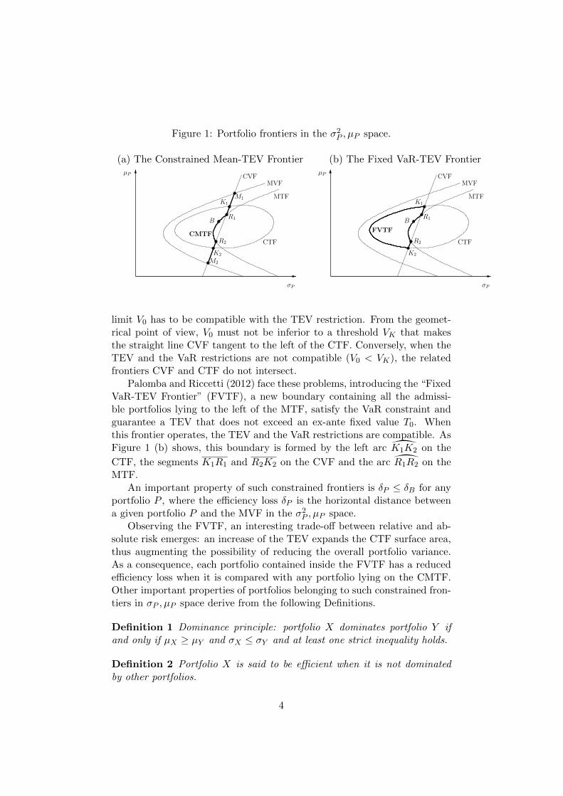
Figure 1: Portfolio frontiers in the σ2P , µP space.

(a) The Constrained Mean-TEV Frontier (b) The Fixed VaR-TEV FrontierµP

σP

MTF

MVF

CTF

CVF

B

M2

M1

R2

K1

K2

R1

CMTF

µP

σP

MTF

MVF

CTF

CVF

B

R2

K1

K2

R1

FVTF

limit V0 has to be compatible with the TEV restriction. From the geomet-rical point of view, V0 must not be inferior to a threshold VK that makesthe straight line CVF tangent to the left of the CTF. Conversely, when theTEV and the VaR restrictions are not compatible (V0 < VK), the relatedfrontiers CVF and CTF do not intersect.

Palomba and Riccetti (2012) face these problems, introducing the “FixedVaR-TEV Frontier” (FVTF), a new boundary containing all the admissi-ble portfolios lying to the left of the MTF, satisfy the VaR constraint andguarantee a TEV that does not exceed an ex-ante fixed value T0. Whenthis frontier operates, the TEV and the VaR restrictions are compatible. AsFigure 1 (b) shows, this boundary is formed by the left arc K1K2 on the

CTF, the segments K1R1 and R2K2 on the CVF and the arc R1R2 on theMTF.

An important property of such constrained frontiers is δP ≤ δB for anyportfolio P , where the efficiency loss δP is the horizontal distance betweena given portfolio P and the MVF in the σ2P , µP space.

Observing the FVTF, an interesting trade-off between relative and ab-solute risk emerges: an increase of the TEV expands the CTF surface area,thus augmenting the possibility of reducing the overall portfolio variance.As a consequence, each portfolio contained inside the FVTF has a reducedefficiency loss when it is compared with any portfolio lying on the CMTF.Other important properties of portfolios belonging to such constrained fron-tiers in σP , µP space derive from the following Definitions.

Definition 1 Dominance principle: portfolio X dominates portfolio Y ifand only if µX ≥ µY and σX ≤ σY and at least one strict inequality holds.

Definition 2 Portfolio X is said to be efficient when it is not dominatedby other portfolios.

4

Accordingly, for any expected return µK2 ≤ µP < µK1 , where portfoliosK1 and K2 are the intersections between the elliptical frontier and the linearboundary CVF, the following properties emerge:

• all portfolios belonging to the CMTF are not dominated by thosebelonging to the MTF,

• all portfolios belonging to the FVTF are not dominated by those be-longing to the CMTF.

Briefly, when the asset manager has to face restrictions on maximumTEV and VaR which are not compatible, the fund has no way of existingbecause the VaR line CVF does not intersect the elliptical CTF; in this sit-uation, the risk management has to modify at least one constraint assignedto the manager. Otherwise, when the maximum TEV and the VaR restric-tions are compatible, portfolios lying on the CMTF are surely dominated.Finally, according to the dominance criterion, an asset manager could investon portfolios contained in the efficient set of the MVF when a TEV limithas not been imposed.

3 The Constrained-Efficient Frontiers

In this section we use the dominance criterion already introduced in Defi-nition 1, in order to focus our attention on the efficient subset of any givenconstrained portfolio frontier. Therefore the notion of portfolio efficiencyis conditional to an existing TEV restriction. Specifically, we propose ananalysis in which managers have to face several risk constraints by selectingonly those admissible portfolios that are non dominated in terms of absoluterisk and expected return.

Before starting the analysis, some notation has to be provided. Given nrisky assets with expected returns µ and variance-covariance matrix Ω, thefollowing constants are defined: a = ι′Ω−1ι, b = ι′Ω−1µ, c = µ′Ω−1µ andd = c−b2/a, where ι is a n-dimensional column vector in which each elementis 1. The minimum variance portfolio of the “mean-variance frontier” C hasexpected return µC = b/a and variance σ2C = 1/a. All these values are inde-pendent of managers’ strategies because they are derived exclusively fromthe available data. The benchmark portfolio is B ≡ (σ2B, µB). In order tosave space, we assume the parameter ∆1 = µB−µC strictly positive. Underthese conditions, the slope of the CTF horizontal axis is positive. More-over, all the analysis will be carried out by imposing the TEV restrictionT0 < δB = ∆2−∆2

1/d, where ∆2 = σ2B−σ2C , which prevents any intersectionbetween the CTF and the MVF.

5

3.1 The Efficient Constrained TEV Frontier (ECTF)

Definition 3 The “Efficient Constrained TEV Frontier” (ECTF) is the setof portfolios that are on the “Constrained TEV Frontier” (CTF) and are notdominated in mean-variance terms.

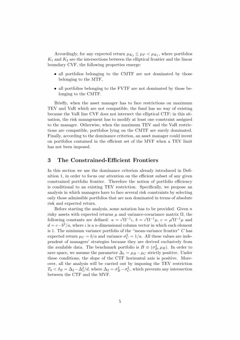
Figure 2: The Efficient Constrained TEV Frontier (ECTF)

µP

σP

MTF

MVF

CTF

J0

J1

ECTF

In practice, the ECTF corresponds to the upper arc J0J1 on the CTFwhere the TEV assumes its maximum value T0, as Figure 2 clearly shows.In the σ2P , µP space, the extremal portfolio

J0 ≡(σ2B + T0 − 2

√T0∆2, µB −∆1

»T0/∆2

)(3)

is that of minimum variance, while the portfolio

J1 ≡(σ2B + T0 + 2∆1

»T0/d, µB +

√dT0

)(4)

corresponds to the intersection between the CTF and the MTF, which rep-resents the portfolio with the highest expected return available. Analyticaldetails about these portfolios are provided by Jorion (2003), while someuseful properties regarding J0 are provided in Appendix A-2.

It is worth noting that the TEV restriction enters equations (3) and

(4), thus determining the position of the arc J0J1. When T0 = 0 the twoportfolios collapse to the benchmark,4 therefore J0 ≡ J1 ≡ B; otherwise,the expected return and the absolute risk of portfolio J1 are always greaterthan those of portfolio J0, independently of the horizontal slope of the CTF.

4In short: the following relationships

- µJ1 − µJ0 ≥ 0 ⇒√T0[√d+ ∆1/

√∆2] ≥ 0

- σJ1 − σJ0 ≥ 0 ⇒ 2√T0[∆1/

√d+√

∆2] ≥ 0

are true by construction for any ∆1.

6

The concept of constrained-efficiency could be extended from the mean-variance efficiency to the mean-VaR or the mean-CVaR (Conditional Value-at-Risk) efficiency. Indeed, the mean-VaR efficient frontier is a proper subsetof the mean-CVaR efficient frontier which, in turn, is a proper subset of theefficient set of the MVF (for a detailed discussion, see Alexander, 2009).

3.2 The Efficient Constrained TEV-Variance Frontier (ECTVF)

Definition 4 The “Efficient Constrained TEV-Variance Frontier” (here-after ECTVF) is the subset of the ECTF in which all portfolios have avariance not superior to a maximum threshold (σ20).

Let S0 be a reference portfolio in the σ2P , µP space, which lies inside theCTF and for which the overall portfolio variance must belong to the intervalσ2J0 ≤ σ20 ≤ σ2J1 , therefore

σ2B + T0 − 2√T0∆2 ≤ σ20 ≤ σ2B + T0 + 2∆1

»T0/d. (5)

This condition is crucial to have a constraint on portfolio variance. Forinstance, the restriction σ20 < σ2J0 does not permit to satisfy the conditionTEV≤ T0, while choosing a portfolio with σ20 > σ2J1 does not produce anyrestriction to the ECTF. Geometrically, the variance constraint correspondsto a vertical line crossing the CTF in two portfolios, namely S2 and the TEVefficient S1 ≡ (σ20, µS1). In practice, the ECTVF consists of the arc startingfrom portfolio J0 to S1. Clearly, when σ20 = σ2J1 the ECTVF and the ECTFcoincide. For simplicity and without any loss of generality, Figure 3 showsthe case of S0 ≡ B for which σ20 = σ2B is the variance associated to thebenchmark.5

3.3 Efficient Fixed VaR-TEV Frontier (EFVTF)

Definition 5 The “Efficient Fixed VaR-TEV Frontier” (EFVTF) is thesubset of the ECTF in which all portfolios have a VaR not superior to amaximum threshold (V0).

The EFVTF is the subset of the ECTF which lies to the left of thestraight line CVF; in practice, it is given by the intersection between theFVTF and the ECTF. In this context, the condition

VK ≤ V0 ≤ maxVJ0 , VJ1 (6)

5For example, Jorion (2003) shows that, if the restriction σ0 = σB is imposed, theexpected return on the CTF is

µS1 = µB − T0∆1

2∆2+

T0

Åd− ∆2

1

∆2

ã(1− T0

4∆2

).

7

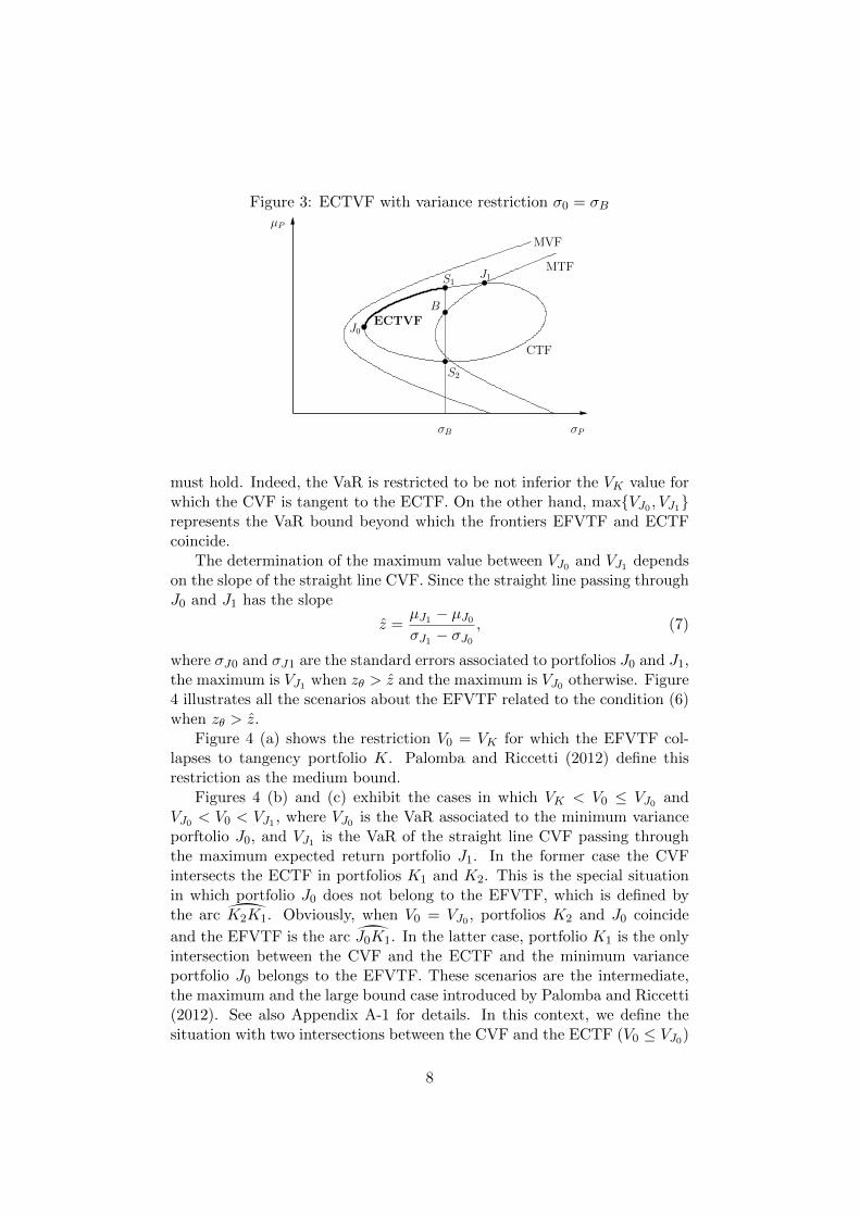
Figure 3: ECTVF with variance restriction σ0 = σBµP

σP

MTF

MVF

CTF

J0

σB

ECTVFB

J1S1

S2

must hold. Indeed, the VaR is restricted to be not inferior the VK value forwhich the CVF is tangent to the ECTF. On the other hand, maxVJ0 , VJ1represents the VaR bound beyond which the frontiers EFVTF and ECTFcoincide.

The determination of the maximum value between VJ0 and VJ1 dependson the slope of the straight line CVF. Since the straight line passing throughJ0 and J1 has the slope

z =µJ1 − µJ0σJ1 − σJ0

, (7)

where σJ0 and σJ1 are the standard errors associated to portfolios J0 and J1,the maximum is VJ1 when zθ > z and the maximum is VJ0 otherwise. Figure4 illustrates all the scenarios about the EFVTF related to the condition (6)when zθ > z.

Figure 4 (a) shows the restriction V0 = VK for which the EFVTF col-lapses to tangency portfolio K. Palomba and Riccetti (2012) define thisrestriction as the medium bound.

Figures 4 (b) and (c) exhibit the cases in which VK < V0 ≤ VJ0 andVJ0 < V0 < VJ1 , where VJ0 is the VaR associated to the minimum varianceporftolio J0, and VJ1 is the VaR of the straight line CVF passing throughthe maximum expected return portfolio J1. In the former case the CVFintersects the ECTF in portfolios K1 and K2. This is the special situationin which portfolio J0 does not belong to the EFVTF, which is defined bythe arc K2K1. Obviously, when V0 = VJ0 , portfolios K2 and J0 coincide

and the EFVTF is the arc J0K1. In the latter case, portfolio K1 is the onlyintersection between the CVF and the ECTF and the minimum varianceportfolio J0 belongs to the EFVTF. These scenarios are the intermediate,the maximum and the large bound case introduced by Palomba and Riccetti(2012). See also Appendix A-1 for details. In this context, we define thesituation with two intersections between the CVF and the ECTF (V0 ≤ VJ0)

8

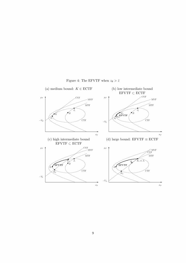
Figure 4: The EFVTF when zθ > z

(a) medium bound: K ∈ ECTF (b) low intermediate boundEFVTF ⊂ ECTF

MTF

CTF

µPMVF

σP

J1BK

−VK

CVF

J0

MTF

CTF

µPMVF

σP

J1BK1

J0

EFVTF

CVF

K2

−V0

(c) high intermediate bound (d) large bound: EFVTF ≡ ECTFEFVTF ⊂ ECTF

MTF

CTF

µPMVF

σP

−V0

J1

CVF

B

J0

K1

EFVTF

K2

MTF

CTF

µPMVF

K1 ≡ J1

σP

CVF

−VJ1

EFVTF

B

J0

K2

9

as the low intermediate bound, while the situation with a single intersection(V0 > VJ0) corresponds to the high intermediate bound.

Figure 4 (d) shows the large bound case V0 = VJ1 under which thestraight line CVF passes through the portfolio J1 and the EFVTF and theECTF coincide; the same situation is also available when V0 > VJ1 becausethe VaR constraint is not binding for the ECTF.

Clearly, under the condition zθ < z, the VaR restrictions change asfollows:

- low intermediate bound (VK < V0 ≤ VJ1): the EFVTF is the arc K1K2

or the arc J1K2 in the special case V0 = VJ1 ;

- high intermediate bound (VJ1 < V0 < VJ0): the EFVTF is the arc

J1K2;

- large bound (V0 ≥ VJ0): EFTVF ≡ ECTF.

3.4 Relationships between efficient frontiers

Once a TEV constraint is set, the restrictions to the overall portfolio varianceor to the VaR necessarily depend on the choice of the reference portfolio S0.

Let such portfolio be non dominated, therefore S0 ∈ ECTF. The inter-section between the linear constraints σP = σ0 and µP = zθσP − V0 lies onthe arc J0J1: this implies that the reference portfolio could be S0 ≡ K1 or,alternatively, S0 ≡ K2, where K1 and K2 are the intersections between theECTF and the linear boundary CVF; more precisely, K1 is the one lyingto the right of the tangency portfolio K, while K2 belongs to the arc J0K.As a consequence, the reference portfolio could be K, J0 or J1 when theVaR is set to the extremal values of the [VK ,maxVJ0 , VJ1] interval. Allthe scenarios are presented in Table 1.

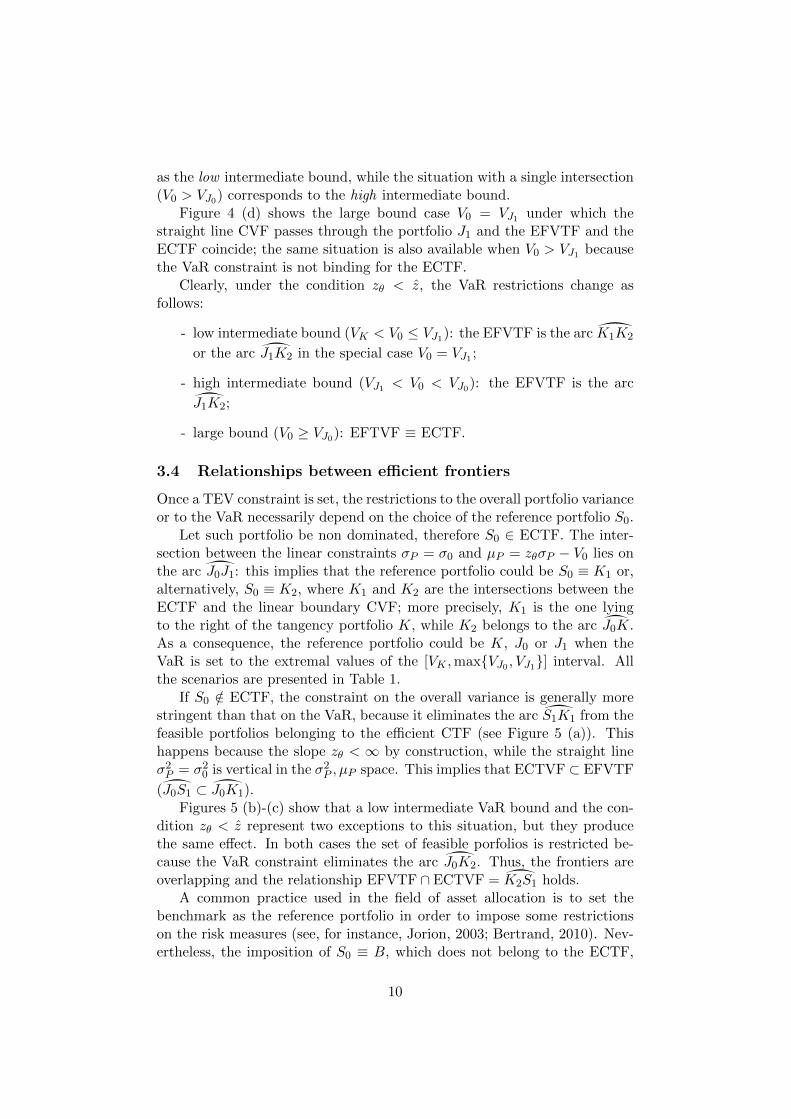
If S0 /∈ ECTF, the constraint on the overall variance is generally morestringent than that on the VaR, because it eliminates the arc S1K1 from thefeasible portfolios belonging to the efficient CTF (see Figure 5 (a)). Thishappens because the slope zθ < ∞ by construction, while the straight lineσ2P = σ20 is vertical in the σ2P , µP space. This implies that ECTVF ⊂ EFVTF

(J0S1 ⊂ J0K1).Figures 5 (b)-(c) show that a low intermediate VaR bound and the con-

dition zθ < z represent two exceptions to this situation, but they producethe same effect. In both cases the set of feasible porfolios is restricted be-cause the VaR constraint eliminates the arc J0K2. Thus, the frontiers areoverlapping and the relationship EFVTF ∩ ECTVF = K2S1 holds.

A common practice used in the field of asset allocation is to set thebenchmark as the reference portfolio in order to impose some restrictionson the risk measures (see, for instance, Jorion, 2003; Bertrand, 2010). Nev-ertheless, the imposition of S0 ≡ B, which does not belong to the ECTF,

10

Figure 5: Variance and VaR constraints when the reference portfolio S0 /∈ECTF

(a) General setup

CTF

B

CVF

J1

MVF

MTF

J0

σB σP

µP

K1

S0

S1

−V0

(b) Low intermediate VaR bound

CVF

σP

µP

−V0

J1

B

S1

S0

K1

CTF

MTF

MVF

σ0

J0

K2

(c) Slope zθ < z

CTF

B

J1

MVF

MTF

J0

σP

µP

CVF

K2S0

−V0

σ0

S1

11

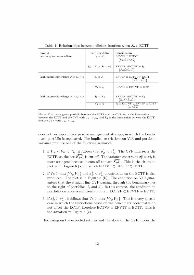
Table 1: Relationships between efficient frontiers when S0 ∈ ECTF

bound ref. portfolio relationshipmedium/low intermediate S0 ≡ K1 EFVTF ⊂ ECTVF(

K2K1⊂J0K1

)S0 ≡ K or S0 ≡ K2 EFVTF ∩ ECTVF(

S0K1∩J0S0

) = S0

high intermediate/large with zθ ≥ z S0 ≡ K1 EFVTF ≡ ECTVF ⊂ ECTF(J0K1⊂J0J1

)S0 ≡ J1 EFVTF ≡ ECTVF ≡ ECTF

high intermediate/large with zθ < z S0 ≡ K2 EFVTF ∩ ECTVF(K2J1∩J0K2

) = K2

S0 ≡ J0 J0 ≡ ECTVF ⊂ EFVTF(J0∈J0J1

) ≡ ECTF

Note: K is the tangency portfolio between the ECTF and the CVF, K1 is the intersectionbetween the ECTF and the CVF with µK1

> µK and K2 is the intersection between the ECTFand the CVF with µK2 < µK .

does not correspond to a passive management strategy, in which the bench-mark portfolio is replicated. The implied restrictions on VaR and portfoliovariance produce one of the following scenarios:

1. if VJ0 < VB < VJ1 , it follows that σ2B < σ2J1 . The CVF intersects the

ECTF, so the arc K1J1 is cut off. The variance constraint σ20 = σ2B is

more stringent because it cuts off the arc S1J1. This is the situationplotted in Figure 6 (a), in which ECTVF ⊂ EFVTF ⊂ ECTF.

2. if VB ≥ maxVJ0 , VJ1 and σ2B < σ2J1 a restriction on the ECTF is alsoproduced. The plot is in Figure 6 (b). The condition on VaR guar-antees that the straight line CVF passing through the benchmark liesto the right of portfolios J0 and J1. In this context, the condition onportfolio variance is sufficient to obtain ECTVF ⊂ EFVTF ≡ ECTF;

3. if σ2B ≥ σ2J1 , it follows that VB ≥ maxVJ0 , VJ1. This is a very specialcase in which the restrictions based on the benchmark coordinates donot affect the ECTF, therefore ECTVF ≡ EFVTF ≡ ECTF. This isthe situation in Figure 6 (c).

Focussing on the expected returns and the slope of the CVF, under the

12

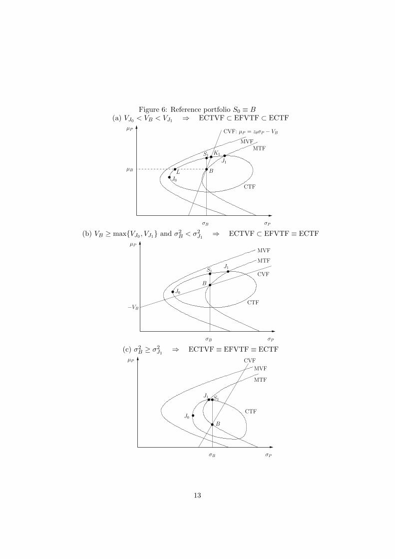
Figure 6: Reference portfolio S0 ≡ B(a) VJ0 < VB < VJ1 ⇒ ECTVF ⊂ EFVTF ⊂ ECTF

µP

σP

MTF

CTF

J1

CVF: µP = zθσP − VB

µB L

σB

S1K1

B

J0

MVF

(b) VB ≥ maxVJ0 , VJ1 and σ2B < σ2J1 ⇒ ECTVF ⊂ EFVTF ≡ ECTF

µP

σP

CTF

B

−VB

σB

J1S1

J0

MTF

MVF

CVF

(c) σ2B ≥ σ2J1 ⇒ ECTVF ≡ EFVTF ≡ ECTF

µP

σP

MTF

B

S1

σB

CTF

J1

MVF

CVF

J0

13

assumption VB > VJ0 , the above conditions can be summarized as follows:6

1. zθ > zγ and µC <µJ1 + µB

2

2. zθ ≤ zγ and µC <µJ1 + µB

2

3. µC ≥µJ1 + µB

2

(8)

where µC is the expected return of the minimum variance portfolio on theMVF and zγ = (µJ1 −µB)/(σJ1 −σB) is the slope of the theoretical straightline passing through portfolios B and J1. From the conditions in (8), onecan observe that:

(a) when ∆1 > 0 (the CTF has positive slope), surely µC ≤µJ1 + µB

2;

(b) when the managers confidence level is low, it follows that zθ <√d

(see Alexander and Baptista, 2008, or Palomba and Riccetti, 2012 fordetails). This always implies VB > VJ1 ;

(c) when T0 > 0, the restriction σ2J1 = σ2B indicates that the straightline passing through portfolios B and J1 is vertical in σP , µP space.Moreover, the condition µC ≥ (µJ1 + µB)/2 is sufficient to obtainVJ1 < VB because the straight line passing through B and J1 is verticalor has a negative slope in σP , µP space, while the CVF slope zθ isgreater than zero by construction.

Analytical details about all these relationships are provided in AppendixA-4.

3.5 VaR and variance bounds in presence of a TEV con-straint

The aim of this section is to show how it is possible to set a constraint tothe overall portfolio variance or to the VaR in presence of a TEV restric-tion already imposed to asset managers. In particular, we are interested toexamine how the constrained portfolio variance σ2S0

∈ [σ2J0 , σ2J1

] and the con-strained VaR V0 ∈ [VK ,maxVJ0 , VJ1] can restrict the number of feasibleportfolios lying on the efficient CTF. In doing so, we focus on the followingportfolios:

1. J1 is that of maximum expected return or Information Ratio (IR=(µP − µB)/T0, see for instance Lee, 2000);

6In practice, in our discussion the condition VB < VJ0 is avoided because it correspondsto a very special situation in which the straight line CVF is approximately horizontal inσP , µP space.

14

2. J0 is that of minimum absolute risk;

3. K is that for which the VaR is minimised;

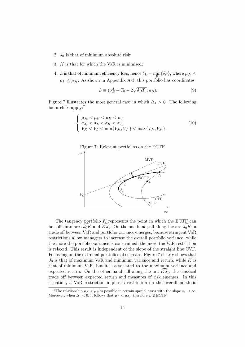
4. L is that of minimum efficiency loss, hence δL = minPδP , where µJ0 ≤

µP ≤ µJ1 . As shown in Appendix A-3, this portfolio has coordinates

L ≡ (σ2B + T0 − 2√δBT0, µB). (9)

Figure 7 illustrates the most general case in which ∆1 > 0. The followinghierarchies apply:7

µJ0 < µB < µK < µJ1σJ0 < σL < σK < σJ1VK < VL < minVJ0 , VJ1 < maxVJ0 , VJ1.

(10)

Figure 7: Relevant portfolios on the ECTFµP

σP

B

J1

L

J0

K

CVFMVF

CTFMTF

ECTF

−VK

The tangency portfolio K represents the point in which the ECTF canbe split into arcs J0K and KJ1. On the one hand, all along the arc J0K, atrade off between VaR and portfolio variance emerges, because stringent VaRrestrictions allow managers to increase the overall portfolio variance, whilethe more the portfolio variance is constrained, the more the VaR restrictionis relaxed. This result is independent of the slope of the straight line CVF.Focussing on the extremal portfolios of such arc, Figure 7 clearly shows thatJ0 is that of maximum VaR and minimum variance and return, while K isthat of minimum VaR, but it is associated to the maximum variance andexpected return. On the other hand, all along the arc KJ1, the classicaltrade off between expected return and measures of risk emerges. In thissituation, a VaR restriction implies a restriction on the overall portfolio

7The relationship µK < µB is possible in certain special cases with the slope zθ →∞.Moreover, when ∆1 < 0, it follows that µB < µJ0 , therefore L /∈ ECTF.

15

variance and viceversa. The extremal position J1 is available only when theconstraints on the absolute risk measures are absent or non binding.

If managers’ aim is to minimise the portfolio efficiency loss on the ECTF,they can invest on portfolio L. It allows them to replicate the benchmarkreturn and also to reduce the measures of risk because σ2L < σ2B and VL <VB. Furthermore, from the risk perpective, this choice is often convenientbecause the restrictions on the VaR and the variance have been set close totheir minimum values.

3.6 An empirical example

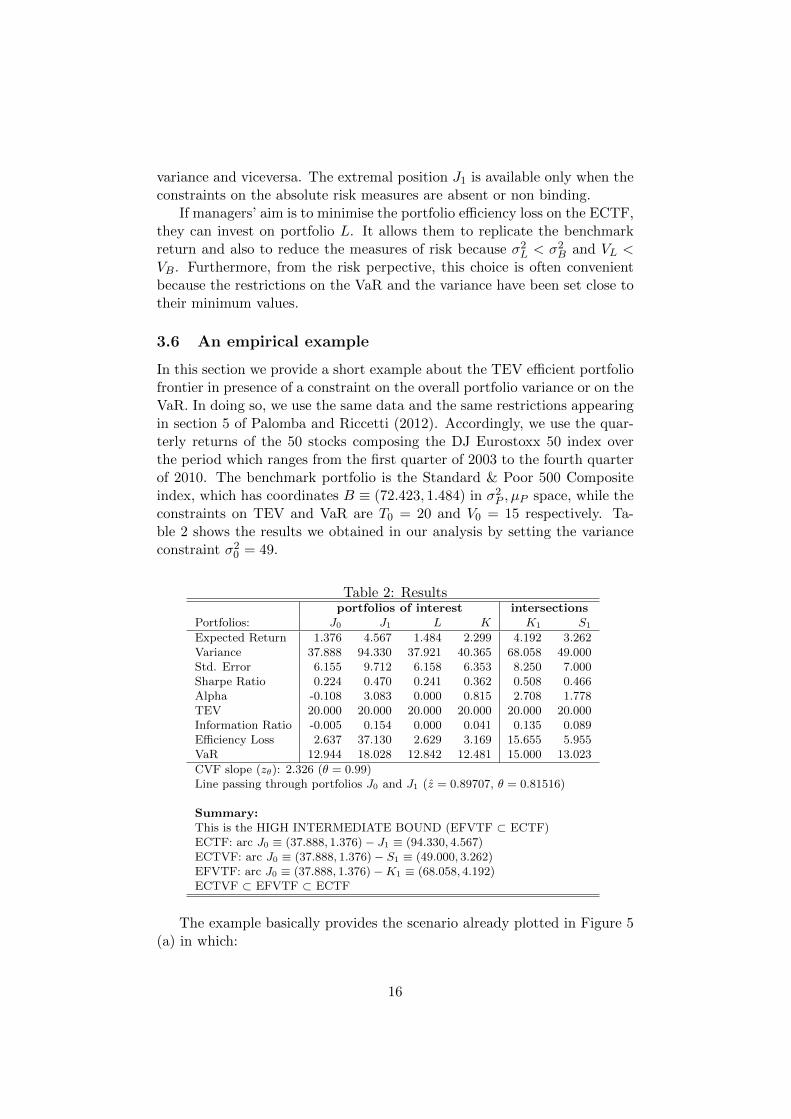
In this section we provide a short example about the TEV efficient portfoliofrontier in presence of a constraint on the overall portfolio variance or on theVaR. In doing so, we use the same data and the same restrictions appearingin section 5 of Palomba and Riccetti (2012). Accordingly, we use the quar-terly returns of the 50 stocks composing the DJ Eurostoxx 50 index overthe period which ranges from the first quarter of 2003 to the fourth quarterof 2010. The benchmark portfolio is the Standard & Poor 500 Compositeindex, which has coordinates B ≡ (72.423, 1.484) in σ2P , µP space, while theconstraints on TEV and VaR are T0 = 20 and V0 = 15 respectively. Ta-ble 2 shows the results we obtained in our analysis by setting the varianceconstraint σ20 = 49.

Table 2: Resultsportfolios of interest intersections

Portfolios: J0 J1 L K K1 S1

Expected Return 1.376 4.567 1.484 2.299 4.192 3.262Variance 37.888 94.330 37.921 40.365 68.058 49.000Std. Error 6.155 9.712 6.158 6.353 8.250 7.000Sharpe Ratio 0.224 0.470 0.241 0.362 0.508 0.466Alpha -0.108 3.083 0.000 0.815 2.708 1.778TEV 20.000 20.000 20.000 20.000 20.000 20.000Information Ratio -0.005 0.154 0.000 0.041 0.135 0.089Efficiency Loss 2.637 37.130 2.629 3.169 15.655 5.955VaR 12.944 18.028 12.842 12.481 15.000 13.023

CVF slope (zθ): 2.326 (θ = 0.99)Line passing through portfolios J0 and J1 (z = 0.89707, θ = 0.81516)

Summary:This is the HIGH INTERMEDIATE BOUND (EFVTF ⊂ ECTF)ECTF: arc J0 ≡ (37.888, 1.376)− J1 ≡ (94.330, 4.567)ECTVF: arc J0 ≡ (37.888, 1.376)− S1 ≡ (49.000, 3.262)EFVTF: arc J0 ≡ (37.888, 1.376)−K1 ≡ (68.058, 4.192)ECTVF ⊂ EFVTF ⊂ ECTF

The example basically provides the scenario already plotted in Figure 5(a) in which:

16

(a) there is only one intersection between the ECTF and the straight lineCVF, provided by portfolio K1. Accordingly, this is the high interme-diate bound. The other intersection between the CVF and the ellipti-cal boundary CTF is K2 ≡ (42.432, 0.154), which lies below portfolioJ0;

(b) the constraint on the variance portfolio is more stringent than thatimposed to the VaR. This implies that the intersection K1 lies to theright of S1. Since both restrictions cut off a portion of the arc J0J1containing J1, the relationship ECTVF ⊂ EFVTF ⊂ ECTF holds;

(c) the restrictions V0 = 15 and σ20 = 49 do not exclude J0, K, L from theconstrained set of TEV efficient portfolios;

(d) portfolios K1 and S1 become those with the maximum expected re-turn/IR under V0 = 15 and σ20 = 49 respectively.

Finally, using the benchmark as the reference portfolio, the variance andthe VaR restrictions become σ2B = 72.423 and VB = 18.314. This corre-sponds to the large bound situation (portfolio K1 lies to the right of port-

folio J1), where S1 ≡ (72.423, 4.311) and ECTVF= J0S1. The relationshipamong the three TEV efficient frontiers is ECTVF ⊂ ECTF ≡ EFVTF.

4 Concluding remarks

This paper analyses the situation in which the risk management imposes amaximum TEV constraint to asset managers. Accordingly, Jorion (2003)introduces an elliptical frontier in the traditional mean-variance space con-taining all the constant TEV portfolios.

Nevertheless, many portfolios belonging to the surface area of this fron-tier are overly risky. Jorion (2003) addresses this problem by adding avariance constraint, while Palomba and Riccetti (2012), starting from thework of Alexander and Baptista (2008), insert also a Value-at-Risk (VaR)constraint, thus defining the “Fixed VaR-TEV Frontier” (FVTF), a port-folio boundary which satisfies the VaR constraint and guarantees a TEVthat does not exceed an ex-ante fixed value T0. Provided that the abovementioned frontiers are closed and bounded sets, we focus on their efficientsubset by using the mean-variance dominance criterion; accordingly, we de-fine the “Efficient Constrained TEV Frontier”(ECTF) as the subset on theJorion’s elliptical boundary containing non dominated portfolios. More-over, the imposition of a maximum variance restriction reduces the ECTFto the “Efficient Constrained TEV-Variance Frontier” (ECTVF), while the“Efficient Fixed VaR-TEV Frontier” (EFVTF) arises when a VaR limit isimposed.

17

It is well known that investors aim to maximise their utility which is afunction of the portfolio mean and variance. Therefore they can be inter-ested in maximising the expected return of their portfolios or in minimisingsome measures of risk. Once a maximum TEV is fixed, the risk manage-ment can improve the managed portfolio performance by setting additionalconstraints on the overall portfolio variance or the VaR. In the usual spacewith coordinates given by the portfolio standard deviation and the expectedreturn, these constraints correspond to a straight line which splits the planein two halfplanes: the former restriction produces a vertical line for a fixedstandard deviation, while the latter restriction is represented by the linearboundary “Constrained VaR frontier” (CVF), whose slope zθ > 0 is theθ-quantile of the portfolio distribution that depends on the managers confi-dence level 0.5 < θ < 1. In general, focussing on the TEV efficient portfolios,this property makes the VaR constraint preferable to a variance constraint.In practice, once a reference portfolio is set (usually this is the benchmark),it produces a less stringent effect because the number of portfolios satisfyingthe variance restriction is not superior to the number of the VaR constrainedportfolios.

In this framework, the compatibility between the TEV-efficiency andthe restrictions on risk measures is crucial. In other words, at least onevariance/VaR constrained portfolio must exist or, alternatively, at least oneportfolio belonging to the ECTF must lie on the admissible halfplane.

Finally, all the results of our analysis are obtained when the returns areassumed normally distributed and short sales are allowed. Relaxing theseassumptions could make the entire approach more realistic. This could bethe goal of further research.

References

Alexander G. (2009), “From Markowitz to modern risk management”,The European Journal of Finance 15(5-6), pp. 451–461.

Alexander G. and Baptista A. (2008), “Active portfolio managementwith benchmarking: Adding a value-at-risk constraint”, Journal of Eco-nomic Dynamics and Control 32(3), pp. 779–820.

Alexander G. and Baptista A. (2010), “Active portfolio managementwith benchmarking: A frontier based on alpha”, Journal of Banking &Finance 34, pp. 2185–2197.

Bertrand P. (2010), “Another Look at Portfolio Optimization underTracking-Error Constraints”, Financial Analysts Journal 2, pp. 78–90.

Jorion P. (2003), “Portfolio Optimization with Constraints on TrackingError”, Financial Analysts Journal 59(5), pp. 70–82.

18

Lee W. (2000), Advanced Theory and Methodology of Tactical Asset Allo-cation, John Wiley, New York.

Markowitz H. (1952), “Portfolio Selection”, The Journal of Finance 7,pp. 77–91.

Palomba G. and Riccetti L. (2012), “Portfolio Frontiers with Restric-tions to Tracking Error Volatility and Value at Risk”, Journal of Bankingand Finance 36(9).

Roll R. (1992), “A mean/variance analysis of tracking error”, The Journalof Portfolio Management 18(4), pp. 13–22.

Appendix

A-1 Portfolio frontiers

In this section we summarize the analytical definitions in σ2P , µP space of allportfolio frontiers used in our analysis.

A. Classical frontiers

MVF - Mean-variance Frontier (Markowitz, 1952):

σ2P = σ2C +1

d(µP − µC)2 (A-1)

MTF - Mean-TEV Frontier (Roll, 1992):

σ2P = σ2B +1

d(µP − µB)2 + 2

∆1

d(µP − µB) (A-2)

CTF - Constrained TEV Frontier (Jorion, 2003):

d(σ2P − σ2B − T0)2 + 4∆2(µP − µB)2 +

−4∆1(σ2P − σ2B − T0)(µP − µB)− 4dδBT0 = 0 (A-3)

CVF - Constrained VaR Frontier (Alexander and Baptista, 2008):

σ2P =

ŵP + V0zθ

ã2(A-4)

19

B. VaR depending frontiers

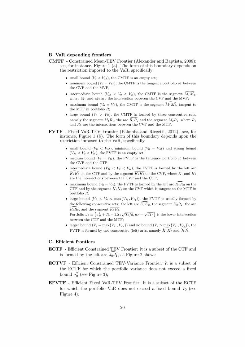
CMTF - Constrained Mean-TEV Frontier (Alexander and Baptista, 2008):see, for instance, Figure 1 (a). The form of this boundary depends onthe restriction imposed to the VaR, specifically

• small bound (V0 < VM ), the CMTF is an empty set;

• minimum bound (V0 = VM ), the CMTF is the tangency portfolio M betweenthe CVF and the MVF,

• intermediate bound (VM < V0 < VR), the CMTF is the segment M1M2,where M1 and M2 are the intersection between the CVF and the MVF;

• maximum bound (V0 = VR), the CMTF is the segment M1M2, tangent tothe MTF in portfolio R;

• large bound (V0 > VR), the CMTF is formed by three consecutive sets,

namely the segment M1R1, the arc R1R2 and the segment M2R2, where R1

and R2 are the intersections between the CVF and the MTF.

FVTF - Fixed VaR-TEV Frontier (Palomba and Riccetti, 2012): see, forinstance, Figure 1 (b). The form of this boundary depends upon therestriction imposed to the VaR, specifically

• small bound (V0 < VM ), minimum bound (V0 = VM ) and strong bound(VM < V0 < VK), the FVTF is an empty set;

• medium bound (V0 = VK), the FVTF is the tangency portfolio K betweenthe CVF and the CTF;

• intermediate bound (VK < V0 < VR), the FVTF is formed by the left arc

K1K2 on the CTF and by the segment K1K2 on the CVF, where K1 and K2

are the intersections between the CVF and the CTF;

• maximum bound (V0 = VR), the FVTF is formed by the left arc K1K2 on theCTF and by the segment K1K2 on the CVF which is tangent to the MTF inportfolio R;

• large bound (VR < V0 < maxVJ1 , VJ2), the FVTF is usually formed by

the following consecutive sets: the left arc K1K2, the segment K2R2, the arc

R1R2, and the segment K1R1.

Portfolio J2 ≡Äσ2B + T0 − 2∆1

√T0/d, µB +

√dT0

äis the lower intersection

between the CTF and the MTF;

• larger bound (V0 = maxVJ1 , VJ2) and no bound (V0 > maxVJ1 , VJ2), the

FVTF is formed by two consecutive (left) arcs, namely K1K2 and J1J2.

C. Efficient frontiers

ECTF - Efficient Constrained TEV Frontier: it is a subset of the CTF andis formed by the left arc J0J1, as Figure 2 shows;

ECTVF - Efficient Constrained TEV-Variance Frontier: it is a subset ofthe ECTF for which the portfolio variance does not exceed a fixedbound σ20 (see Figure 3);

EFVTF - Efficient Fixed VaR-TEV Frontier: it is a subset of the ECTFfor which the portfolio VaR does not exceed a fixed bound V0 (seeFigure 4).

20

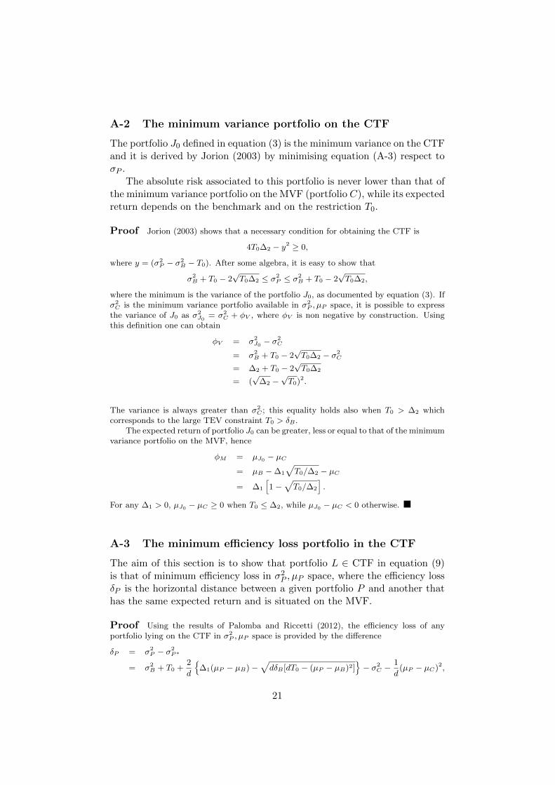
A-2 The minimum variance portfolio on the CTF

The portfolio J0 defined in equation (3) is the minimum variance on the CTFand it is derived by Jorion (2003) by minimising equation (A-3) respect toσP .

The absolute risk associated to this portfolio is never lower than that ofthe minimum variance portfolio on the MVF (portfolio C), while its expectedreturn depends on the benchmark and on the restriction T0.

Proof Jorion (2003) shows that a necessary condition for obtaining the CTF is

4T0∆2 − y2 ≥ 0,

where y = (σ2P − σ2

B − T0). After some algebra, it is easy to show that

σ2B + T0 − 2

√T0∆2 ≤ σ2

P ≤ σ2B + T0 − 2

√T0∆2,

where the minimum is the variance of the portfolio J0, as documented by equation (3). Ifσ2C is the minimum variance portfolio available in σ2

P , µP space, it is possible to expressthe variance of J0 as σ2

J0= σ2

C + φV , where φV is non negative by construction. Usingthis definition one can obtain

φV = σ2J0 − σ

2C

= σ2B + T0 − 2

√T0∆2 − σ2

C

= ∆2 + T0 − 2√T0∆2

= (√

∆2 −√T0)2.

The variance is always greater than σ2C ; this equality holds also when T0 > ∆2 which

corresponds to the large TEV constraint T0 > δB .The expected return of portfolio J0 can be greater, less or equal to that of the minimum

variance portfolio on the MVF, hence

φM = µJ0 − µC= µB −∆1

√T0/∆2 − µC

= ∆1

î1−

√T0/∆2

ó.

For any ∆1 > 0, µJ0 − µC ≥ 0 when T0 ≤ ∆2, while µJ0 − µC < 0 otherwise.

A-3 The minimum efficiency loss portfolio in the CTF

The aim of this section is to show that portfolio L ∈ CTF in equation (9)is that of minimum efficiency loss in σ2P , µP space, where the efficiency lossδP is the horizontal distance between a given portfolio P and another thathas the same expected return and is situated on the MVF.

Proof Using the results of Palomba and Riccetti (2012), the efficiency loss of anyportfolio lying on the CTF in σ2

P , µP space is provided by the difference

δP = σ2P − σ2

P∗

= σ2B + T0 +

2

d

¶∆1(µP − µB)−

√dδB [dT0 − (µP − µB)2]

©− σ2

C −1

d(µP − µC)2,

21

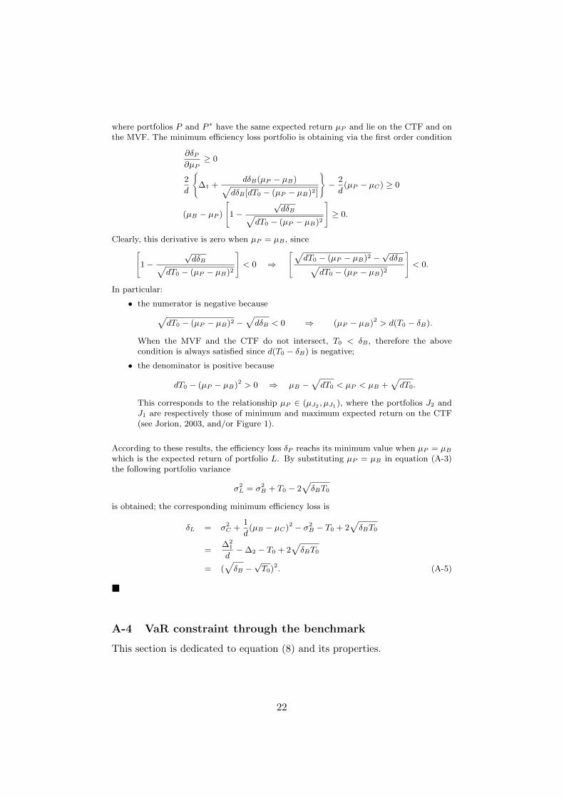
where portfolios P and P ∗ have the same expected return µP and lie on the CTF and onthe MVF. The minimum efficiency loss portfolio is obtaining via the first order condition

∂δP∂µP

≥ 0

2

d

®∆1 +

dδB(µP − µB)√dδB [dT0 − (µP − µB)2]

´− 2

d(µP − µC) ≥ 0

(µB − µP )

ñ1−

√dδB√

dT0 − (µP − µB)2

ô≥ 0.

Clearly, this derivative is zero when µP = µB , sinceñ1−

√dδB√

dT0 − (µP − µB)2

ô< 0 ⇒

ñ√dT0 − (µP − µB)2 −

√dδB√

dT0 − (µP − µB)2

ô< 0.

In particular:

• the numerator is negative because√dT0 − (µP − µB)2 −

√dδB < 0 ⇒ (µP − µB)2 > d(T0 − δB).

When the MVF and the CTF do not intersect, T0 < δB , therefore the abovecondition is always satisfied since d(T0 − δB) is negative;

• the denominator is positive because

dT0 − (µP − µB)2 > 0 ⇒ µB −√dT0 < µP < µB +

√dT0.

This corresponds to the relationship µP ∈ (µJ2 , µJ1), where the portfolios J2 andJ1 are respectively those of minimum and maximum expected return on the CTF(see Jorion, 2003, and/or Figure 1).

According to these results, the efficiency loss δP reachs its minimum value when µP = µBwhich is the expected return of portfolio L. By substituting µP = µB in equation (A-3)the following portfolio variance

σ2L = σ2

B + T0 − 2√δBT0

is obtained; the corresponding minimum efficiency loss is

δL = σ2C +

1

d(µB − µC)2 − σ2

B − T0 + 2√δBT0

=∆2

1

d−∆2 − T0 + 2

√δBT0

= (√δB −

√T0)2. (A-5)

A-4 VaR constraint through the benchmark

This section is dedicated to equation (8) and its properties.

22

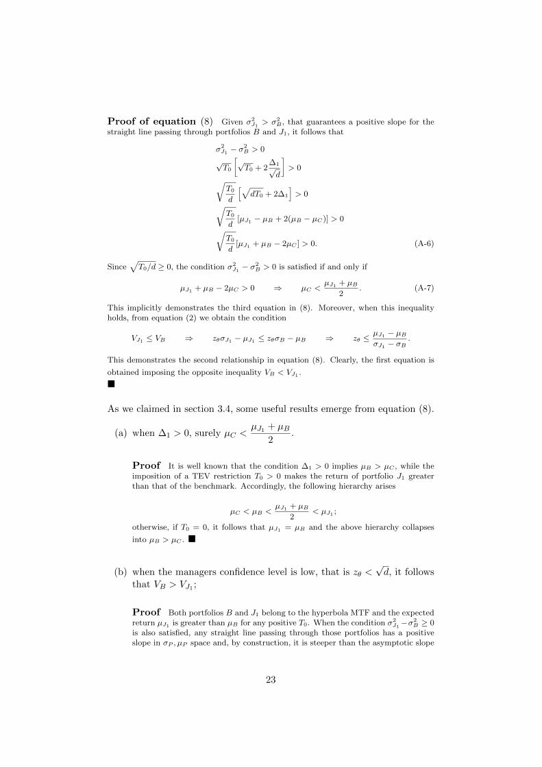
Proof of equation (8) Given σ2J1> σ2

B , that guarantees a positive slope for thestraight line passing through portfolios B and J1, it follows that

σ2J1 − σ

2B > 0

√T0

ï√T0 + 2

∆1√d

ò> 0…

T0

d

î√dT0 + 2∆1

ó> 0…

T0

d[µJ1 − µB + 2(µB − µC)] > 0…

T0

d[µJ1 + µB − 2µC ] > 0. (A-6)

Since√T0/d ≥ 0, the condition σ2

J1− σ2

B > 0 is satisfied if and only if

µJ1 + µB − 2µC > 0 ⇒ µC <µJ1 + µB

2. (A-7)

This implicitly demonstrates the third equation in (8). Moreover, when this inequalityholds, from equation (2) we obtain the condition

VJ1 ≤ VB ⇒ zθσJ1 − µJ1 ≤ zθσB − µB ⇒ zθ ≤µJ1 − µBσJ1 − σB

.

This demonstrates the second relationship in equation (8). Clearly, the first equation is

obtained imposing the opposite inequality VB < VJ1 .

As we claimed in section 3.4, some useful results emerge from equation (8).

(a) when ∆1 > 0, surely µC <µJ1 + µB

2.

Proof It is well known that the condition ∆1 > 0 implies µB > µC , while theimposition of a TEV restriction T0 > 0 makes the return of portfolio J1 greaterthan that of the benchmark. Accordingly, the following hierarchy arises

µC < µB <µJ1 + µB

2< µJ1 ;

otherwise, if T0 = 0, it follows that µJ1 = µB and the above hierarchy collapses

into µB > µC .

(b) when the managers confidence level is low, that is zθ <√d, it follows

that VB > VJ1 ;

Proof Both portfolios B and J1 belong to the hyperbola MTF and the expectedreturn µJ1 is greater than µB for any positive T0. When the condition σ2

J1−σ2

B ≥ 0is also satisfied, any straight line passing through those portfolios has a positiveslope in σP , µP space and, by construction, it is steeper than the asymptotic slope

23

of the MTF (√d).

Moreover, in general it is possible to demonstrate also that the relationship

µJ1 − µBσJ1 − σB

>√d

is always true. Indeed, using some algebra:

µJ1 − µBσJ1 − σB

>√d

√dT0

σJ1 − σB>√d

√T0 + σB > σJ1

T0 + σ2B + 2

√T0σB > σ2

B + T0 + 2∆1

√T0/d

σB >∆1√d

µC +√dσB > µB (A-8)

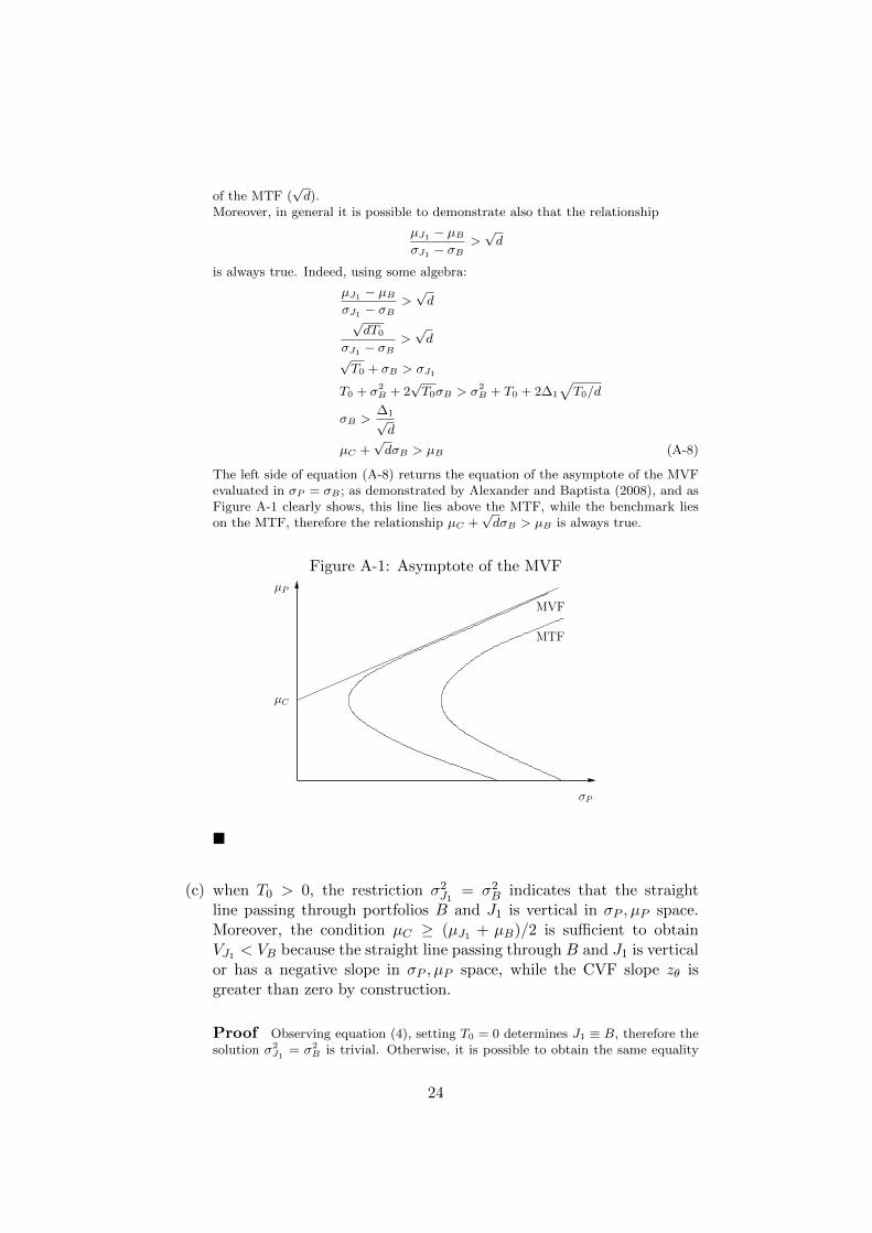
The left side of equation (A-8) returns the equation of the asymptote of the MVFevaluated in σP = σB ; as demonstrated by Alexander and Baptista (2008), and asFigure A-1 clearly shows, this line lies above the MTF, while the benchmark lieson the MTF, therefore the relationship µC +

√dσB > µB is always true.

Figure A-1: Asymptote of the MVFµP

σP

µC

MVF

MTF

(c) when T0 > 0, the restriction σ2J1 = σ2B indicates that the straightline passing through portfolios B and J1 is vertical in σP , µP space.Moreover, the condition µC ≥ (µJ1 + µB)/2 is sufficient to obtainVJ1 < VB because the straight line passing through B and J1 is verticalor has a negative slope in σP , µP space, while the CVF slope zθ isgreater than zero by construction.

Proof Observing equation (4), setting T0 = 0 determines J1 ≡ B, therefore thesolution σ2

J1= σ2

B is trivial. Otherwise, it is possible to obtain the same equality

24

also when the TEV restriction is T0 > 0. In particular, this is the situation

µC =µJ1 + µB

2. (A-9)

When this condition holds, it follows that J1 ≡ (σB , 2µC −µB), ∆1 = µB−µC < 0

and VJ1 = zθσB + µB − 2µC < zθσB − µB = VB .

A-5 Supplementary material

The programming routines for the analysis carried out in this paper can befound at

http://utenti.dea.univpm.it/palomba/TEV-VaR.html

25