A&A 447, 31–48 (2006)DOI: 10.1051/0004-6361:20054185c© ESO 2006

Astronomy&

Astrophysics

The Supernova Legacy Survey: measurement of ΩM, ΩΛ and wfrom the first year data set,

P. Astier1, J. Guy1, N. Regnault1, R. Pain1, E. Aubourg2,3, D. Balam4, S. Basa5, R. G. Carlberg6, S. Fabbro7,D. Fouchez8, I. M. Hook9, D. A. Howell6, H. Lafoux3, J. D. Neill4, N. Palanque-Delabrouille3 , K. Perrett6,

C. J. Pritchet4, J. Rich3, M. Sullivan6, R. Taillet1,10, G. Aldering11, P. Antilogus1, V. Arsenijevic7, C. Balland1,2,S. Baumont1,12, J. Bronder9, H. Courtois13, R. S. Ellis14, M. Filiol5, A. C. Gonçalves15, A. Goobar16, D. Guide1,

D. Hardin1, V. Lusset3, C. Lidman12, R. McMahon17, M. Mouchet15,2, A. Mourao7, S. Perlmutter11,18,P. Ripoche8, C. Tao8, and N. Walton17

(Affiliations can be found after the references)

Received 9 September 2005 / Accepted 11 October 2005

ABSTRACT

We present distance measurements to 71 high redshift type Ia supernovae discovered during the first year of the 5-year Supernova LegacySurvey (SNLS). These events were detected and their multi-color light-curves measured using the MegaPrime/MegaCam instrument at theCanada-France-Hawaii Telescope (CFHT), by repeatedly imaging four one-square degree fields in four bands, as part of the CFHT LegacySurvey (CFHTLS). Follow-up spectroscopy was performed at the VLT, Gemini and Keck telescopes to confirm the nature of the supernovaeand to measure their redshift. With this data set, we have built a Hubble diagram extending to z = 1, with all distance measurements involvingat least two bands. Systematic uncertainties are evaluated making use of the multi-band photometry obtained at CFHT. Cosmological fitsto this first year SNLS Hubble diagram give the following results: ΩM = 0.263 ± 0.042 (stat) ± 0.032 (sys) for a flat ΛCDM model; andw = −1.023 ± 0.090 (stat) ± 0.054 (sys) for a flat cosmology with constant equation of state w when combined with the constraint from therecent Sloan Digital Sky Survey measurement of baryon acoustic oscillations.

Key words. supernovae: general – cosmology: observations – cosmological parameters

Based on observations obtained with MegaPrime/MegaCam, ajoint project of CFHT and CEA/DAPNIA, at the Canada-France-Hawaii Telescope (CFHT) which is operated by the National ResearchCouncil (NRC) of Canada, the Institut National des Sciences del’Univers of the Centre National de la Recherche Scientifique (CNRS)of France, and the University of Hawaii. This work is based inpart on data products produced at the Canadian Astronomy DataCentre as part of the Canada-France-Hawaii Telescope Legacy Survey,a collaborative project of NRC and CNRS. Based on observa-tions obtained at the European Southern Observatory using theVery Large Telescope on the Cerro Paranal (ESO Large Programme171.A-0486). Based on observations (programs GN-2004A-Q-19,GS-2004A-Q-11, GN-2003B-Q-9, and GS-2003B-Q-8) obtained atthe Gemini Observatory, which is operated by the Association ofUniversities for Research in Astronomy, Inc., under a coopera-tive agreement with the NSF on behalf of the Gemini partnership:the National Science Foundation (USA), the Particle Physics andAstronomy Research Council (UK), the National Research Council(Canada), CONICYT (Chile), the Australian Research Council(Australia), CNPq (Brazil) and CONICET (Argentina). Based on ob-servations obtained at the W.M. Keck Observatory, which is op-erated as a scientific partnership among the California Institute ofTechnology, the University of California and the National Aeronautics

1. Introduction

The discovery of the acceleration of the Universe stands as amajor breakthrough of observational cosmology. Surveys ofcosmologically distant Type Ia supernovae (SNe Ia; Riess et al.1998; Perlmutter et al. 1999) indicated the presence of a new,unaccounted-for “dark energy” that opposes the self-attractionof matter and causes the expansion of the Universe to accel-erate. When combined with indirect measurements using cos-mic microwave background (CMB) anisotropies, cosmic shearand studies of galaxy clusters, a cosmological world model hasemerged that describes the Universe as flat, with about 70% ofits energy contained in the form of this cosmic dark energy (seefor example Seljak et al. 2005).

Current projects aim at directly probing the nature of thedark energy via a determination of its equation of state param-eter – the pressure to energy-density ratio – w ≡ pX/ρX , whichalso defines the time dependence of the dark energy density:ρX ∼ a−3(1+w), where a is the scale factor. Recent constraints

and Space Administration. The Observatory was made possible by thegenerous financial support of the W.M. Keck Foundation. Tables 7–9 are only available in electronic form athttp://www.edpsciences.org

Article published by EDP Sciences and available at http://www.edpsciences.org/aa or http://dx.doi.org/10.1051/0004-6361:20054185

32 P. Astier et al. (SNLS Collaboration): SNLS 1st year data set

on w (Knop et al. 2003; Tonry et al. 2003; Barris et al. 2004;Riess et al. 2004) are consistent with a very wide range ofDark Energy models. Among them, the historical cosmolog-ical constant (w = −1) is 10120 to 1060 smaller than plausi-ble vacuum energies predicted by fundamental particle theo-ries. It also cannot explain why matter and dark energy havecomparable densities today. “Dynamical Λ” models have beenproposed (quintessence, k-essence) based on speculative fieldmodels, and some predict values of w above –0.8 – significantlydifferent from –1. Measuring the average value of w with a pre-cision better than 0.1 will permit a discrimination between thenull hypothesis (pure cosmological constant,w = −1) and somedynamical dark energy models.

Improving significantly over current SN constraints on thedark energy requires a ten-fold larger sample (i.e. o(1000) at0.2 < z < 1., where w is best measured), in order to signifi-cantly improve on statistical errors but also, most importantly,on systematic uncertainties. The traditional method of measur-ing distances to SNe Ia involves different types of observationsat about 10 different epochs spread over nearly 3 months: dis-covery via image subtraction, spectroscopic identification, andphotometric follow-up, usually on several telescopes. Many ob-jects are lost or poorly measured in this process due to theeffects of inclement weather during the follow-up observa-tions, and the analysis often subject to largely unknown sys-tematic uncertainties due to the use of various instruments andtelescopes.

The Supernova Legacy Survey (SNLS)1 was designed toimprove significantly over the traditional strategy as follows:1) discovery and photometric follow-up are performed with awide field imager used in “rolling search” mode, where a givenfield is observed every third to fourth night as long as it remainsvisible; 2) service observing is exploited for both spectroscopyand imaging, reducing the impact of bad weather. Using a sin-gle imaging instrument to observe the same fields reduces pho-tometric systematic uncertainties; service observing optimizesboth the yield of spectroscopic observing time, and the light-curve sampling.

In this paper we report the progress made, and the cosmo-logical results obtained, from analyzing the first year of theSNLS. We present the data collected, the precision achievedboth from improved statistics and better control of system-atics, and the potential of the project to further reduce andcontrol systematic uncertainties on cosmological parameters.Section 2 describes the imaging and spectroscopic surveys andtheir current status. Sections 3 and 4 present the data reductionand photometric calibration. The light-curve fitting method, theSNe samples and the cosmological analysis are discussed inSect. 5. A comparison of the nearby and distant samples usedin the cosmological analysis is performed in Sect. 6 and thesystematic uncertainties are discussed in Sect. 7.

2. The Supernova Legacy Survey

The Supernova Legacy Survey is comprised of two compo-nents: an imaging survey to detect SNe and monitor their

1 see http://cfht.hawaii.edu/SNLS/

Table 1. Coordinates and average Milky Way extinction (fromSchlegel et al. 1998) of fields observed by the Deep/SN componentof the CFHTLS.

Field RA(2000) Dec (2000) E(B − V) (MW)

D1 02:26:00.00 –04:30:00.0 0.027

D2 10:00:28.60 +02:12:21.0 0.018

D3 14:19:28.01 +52:40:41.0 0.010

D4 22:15:31.67 –17:44:05.0 0.027

light-curves, and a spectroscopic program to confirm the na-ture of the candidates and measure their redshift.

2.1. The imaging survey

The imaging is taken as part of the deep component of theCFHT Legacy Survey (CFHTLS 2002) using the one squaredegree imager, MegaCam (Boulade et al. 2003). In total,CFHTLS has been allocated 474 nights over 5 years and con-sists of 3 surveys: a very wide shallow survey (1300 squaredegrees), a wide survey (120 square degrees) and a deep sur-vey (4 square degrees). The 4 pointings of the deep surveyare evenly distributed in right ascension (Table 1). The ob-servations for the deep survey are sequenced in a way suit-able for detecting supernovae and measuring their light-curves:in every lunation in which a field is visible, it is imaged atfive equally spaced epochs during a MegaCam run (whichlasts about 18 nights). Observations are taken in a combina-tion of rM, iM plus gM or zM filters (the MegaCam filter set; seeSect. 4) depending on the phase of the moon. Each field is ob-served for 5 to 7 consecutive lunations. Epochs lost to weatheron any one night remain in the queue until the next clear ob-serving opportunity, or until a new observation in the same fil-ter is scheduled.

During the first year of the survey, the observing efficiencywas lower than expected and the nominal observation plancould not always be fulfilled. The scheduled iM exposures(3 × 3600 s plus 2 × 1800 s per lunation) and rM exposures(5 epochs × 1500 s) were usually acquired. Assigned a lowerpriority, gM and zM received less time than originally planned:on average only 2.2 epochs of 1050 s were collected per lu-nation in gM, and 2 epochs of 2700 s in zM; for the latter, theaverage ignores the D2 field and the D3 field in 2003, for whichonly fragmentary observations were obtained in zM. With effi-ciency ramping up, gM and zM approached their nominal ratein May 2004, and since then the nominal observation plan (de-tailed in Sullivan et al. 2005) is usually completed.

Observations and real-time pre-processing are performedby the CFHT staff using the Elixir reduction pipeline (Magnier& Cuillandre 2004), with the data products immediately avail-able to the SN search teams. We have set up two independentreal-time pipelines which analyze these pre-processed images.The detection of new candidates is performed by subtractinga “past" image to the current images, where the past-imageis constructed by stacking previous observations of the samefield. The key element of these pipelines is matching the point

P. Astier et al. (SNLS Collaboration): SNLS 1st year data set 33

spread function of a new exposure to the past-image. This isdone using the Alard algorithm (Alard & Lupton 1998; Alard2000) for one of the pipelines, and using a non-parametric ap-proach for the other. New candidates are detected and measuredon the subtraction images; detections are matched to other de-tections in the field, if any. One of the pipelines processes allbands on an equal footing, the other detects in the iM band(which is deep enough for trigger purposes) and measuresfluxes in the other bands. The two candidate lists are merged af-ter each epoch and typically have an overlap greater than 90%for iM(AB) < 24.0 after two epochs in a dark run. The reasonsfor one candidate being found by only one pipeline are usuallytraced to different masking strategies or different handling ofthe CCD overlap regions.

2.2. Spectroscopic follow-up

Spectroscopy is vital in order to obtain SN redshifts, andto determine the nature of each SN candidate. This re-quires observations on 8−10 m class telescopes due to thefaintness of these distant supernovae. Spectroscopic follow-up time for the candidates presented in this paper was ob-tained at a variety of telescopes during the Spring and Fallsemesters of 2003 and the Spring semester of 2004. The prin-ciple spectroscopic allocations were at the European SouthernObservatory Very Large Telescope (program ID 〈171.A-0486〉;60 h per semester), and at Gemini-North and South (Program-IDs: GN-2004A-Q-19, GS-2004A-Q-11, GN-2003B-Q-9, andGS-2003B-Q-8; 60 h per semester). Spectroscopic time wasalso obtained at Keck-I and Keck-II (3 nights during eachSpring semester) as the D3 field cannot be seen by VLT orGemini-South. Further complementary spectroscopic follow-up observations were also obtained at Keck-I (4 nights in eachof 2003A, 2003B and 2004A) as part of a detailed study of theintermediate redshift SNe in our sample (Ellis et al., in prep.).

Most of the observations are performed in long-slit mode.The detailed spectroscopic classification of these candidates isdiscussed elsewhere (see Howell et al. 2005 and Basa et al.,in prep.). In summary, we consider two classes of events (seeHowell et al. 2005 for the exact definitions): secure SNe Iaevents (“SN Ia”), and probable Ia events (“SN Ia*”), for whichthe spectrum matches a SN Ia better than any other type, butdoes not completely rule out other possible interpretations. Allother events which were not spectroscopically identified asSN Ia or SN Ia* were ignored in this analysis.

The imaging survey still delivers more variable candidatesthan can actually be observed spectroscopically. Hence, an ac-curate ranking of these candidates for further observations isessential. This ranking is performed to optimize the SN Ia yieldof our allocations. Our method uses both a photometric selec-tion tool (discussed in Sullivan et al. 2005) which performsreal-time light-curve fits to reduce the contamination of core-collapse SNe, and a database of every variable object ever de-tected by our pipelines to remove AGN and variable stars whichare seen to vary repeatedly in long-timescale data sets (morethan one year).

SN Ia candidates fainter than iM = 24.5 (likely at z >1) and those with very low percentage increases over theirhost galaxies (where identification is extremely difficult – seeHowell et al. 2005) are usually not observed. With the real-timelight-curve fit technique, approximately 70% of our candidatesturned out to be SNe Ia. The possible biases associated withthis selection were studied in Sullivan et al. (2005) and foundto be negligible.

2.3. The first year data set

The imaging survey started in August 2003 after a fewmonths of MegaCam commissioning. (Some SN candidatespresented here were detected during the commissioning pe-riod.) This paper considers candidates with maximum lightup to July 15th 2004, corresponding approximatively to a fullyear of operation. During this time frame, which includes theramping-up period of the CFHTLS, about 400 transients weredetected, 142 spectra were acquired: 20 events were identi-fied as Type II supernovae, 9 as AGN/QSO, 4 as SN Ib/c,and 91 events were classified as SN Ia or SN Ia*. The 18 re-maining events have inconclusive spectra. Table 7 gives the91 objects identified as SN Ia or SN Ia* during our first yearof operation.

3. Data reduction

3.1. Image preprocessing

At the end of each MegaCam run, the images are pre-processedagain at CFHT using the Elixir pipeline (Magnier & Cuillandre2004). This differs from the real-time reduction process de-scribed in Sect. 2.1, in that master flat-field images and fringe-correction frames are constructed from all available data fromthe entire MegaCam run (including PI data). The Elixir processconsists of flat-fielding and fringe subtraction, with an approxi-mate astrometric solution also derived. Elixir provides reduceddata which has a uniform photometric response across the mo-saic (at the expense of a non-uniform sky background). This“photometric flat-field” correction is constructed using expo-sures with large dithers obtained on dense stellar fields.

The SNLS pipelines then associate a weight map with eachElixir-processed image (i.e. each CCD from a given exposure)from the flat-field frames and the sky background variations.Bad pixels (as identified by Elixir), cosmic rays (detected us-ing the Laplacian filter of van Dokkum 2001), satellite trails,and saturated areas are set to zero in the weight maps. Anobject catalog is then produced using SExtractor (Bertin &Arnouts 1996), and point-like objects are used to derive animage quality (IQ) estimate. The sky background map com-puted by SExtractor is then subtracted from the image. We ad-ditionally perform aperture photometry on the objects of theSExtractor catalog for the purpose of photometric calibration(see Sect. 4).

3.2. Measurement of supernova fluxes

For each supernova candidate, the image with the best IQ (sub-sequently called “reference”) is identified, and all other images

34 P. Astier et al. (SNLS Collaboration): SNLS 1st year data set

(both science images and their weight maps) are resampled tothe pixel grid defined by this reference. The variations of theJacobian of the geometrical transformations, which translateinto photometric non-uniformities in the re-sampled images,are sufficiently small (below the millimag level) to be ignored.We then derive the convolution kernels that would match thePSF (modeled using the DAOPHOT package Stetson 1987) ofthe reference image to the PSF of the other resampled scienceimages, but we do not perform the convolutions. These con-volution kernels not only match the PSFs, but also contain thephotometric ratios of each image to the reference. We ensurethat these photometric ratios are spatially uniform by imposinga spatially uniform kernel integral, but allow for spatial ker-nel shape variations as the images may have spatially varyingPSFs. Following Alard (2000), the kernel is fit on several hun-dred objects selected for their high, though unsaturated, peakflux. The kernel fit is made more robust by excluding objectswith large residuals and iterating.

Our approach to the differential flux measurement of aSN is to simultaneously fit all images in a given filter witha model that includes (i) a spatially variable galaxy (constantwith time), and (ii) a time-variable point source (the super-nova). The model is described in detail in Fabbro (2001). Theshape of the galaxy and positions of both galaxy and supernovaare fit globally. The intensity Di,p in a pixel p of image i ismodeled as:

Di,p =[( fiPref + g) ⊗ ki

]p + bi (1)

where fi are the supernova fluxes, Pref is the PSF of the refer-ence image centered on the SN position; ki is the convolutionkernel that matches the PSF of the reference image to the PSFof image i; g is the intensity of the host galaxy in the refer-ence image, and bi is a local (sky) background in image i. Thenon parametric galaxy “model” g is made of independent pixelswhich represent the galaxy in the best IQ image. All fluxes ( fi)are expressed in units of the reference image flux.

The fit parameters are: the supernova position and thegalaxy pixel values (common to all images), the supernovafluxes, and a constant sky background (different for each im-age). In some images in the series, the supernova flux is knownto be absent or negligible; these frames enter the fit as “zeroflux images” and are thus used to determine the values of thegalaxy pixels. The least-squares photometric fit minimizes:

χ2 =∑i,p

Wi,p (Di,p − Ii,p)2 (2)

where Ii,p and Wi,p are the image and weight values of pixel pin image i, and the sums run over all images that contain theSN position, and all pixels in the fitted stamp of this image.

Note that this method does not involve any real image con-volution: the fitted model possesses the PSF of the referenceimage, and it is the model that is convolved to match the PSFof every other image. We typically fit 50 × 50 galaxy pixelsand several hundred images, and each SN fit usually has 2000to 3000 parameters. The fit is run once, 5σ outlier pixels areremoved, and the fit is run again.

The photometric fit yields values of the fit parameters alongwith a covariance matrix. There are obvious correlations be-tween SN fluxes and galaxy brightness, between these two pa-rameters and the background level, and between the SN posi-tion and the flux, for any given image. More importantly, theuncertainty in the SN position and the galaxy brightness intro-duces correlations between fluxes at different epochs that haveto be taken into account when analyzing the light-curves. Notethat flux variances and the correlations between fluxes decreasewhen adding more “zero flux images” into the fit. It will there-fore be possible to derive an improved photometry for most ofthe events presented in this paper, when the fields are observedagain and more images without SN light are available.

3.3. Flux uncertainties

Once the photometric fit has converged, the parameter covari-ance matrix (including flux variances and covariances) is de-rived. This Section addresses the accuracy of these uncertain-ties, in particular the flux variances and covariances, which areused as inputs to the subsequent light-curve fit.

The normalization of the parameter covariance matrix di-rectly reflects the normalization of image weights. We checkedthat the weights are on average properly normalized becausethe minimum χ2 per degree of freedom is very close to 1 (wefind 1.05 on average). However, this does not imply mathe-matically that the flux uncertainties are properly normalized,because Eq. (2) neglects the correlations between neighbor-ing pixels introduced by image re-sampling. We considered ac-counting for these correlations; however, this would make thefitting code intolerably slow, as the resulting χ2 would be non-diagonal. Using approximate errors in least squares (such asignoring correlations) increases the actual variance of the esti-mators, but in the case considered here, the loss in photometricaccuracy is below 1%. The real drawback of ignoring pixel cor-relations is that parameter uncertainties extracted from the fitare underestimated (since pixel correlations are positive); thisis a product of any photometry method that assumes uncorre-lated pixels on re-sampled or convolved images. Our geometricalignment technique, used to align images prior to the flux mea-surement as described in Sect. 3.2, uses a 3 × 3 pixel quadraticre-sampling kernel, which produces output pixels with an av-erage variance of 80% of the input pixel variance, where theremaining 20% contributes to covariance in nearby pixels. Wechecked that flux variances (and covariances) computed assum-ing independent pixels are also underestimated by the sameamount: on average, a 25% increase is required.

In order to derive accurate uncertainties, we used the factthat for each epoch, several images are available which mea-sure the same object flux. Estimating fluxes on individual ex-posures rather than on stacks per night preserves the photomet-ric precision since a common position is fit using all images.It also allows a check on the consistency of fluxes measuredwithin a night. We therefore fit a common flux per night tothe fluxes measured on each individual image by minimizinga χ2

n (where n stands for nights); this matrix is non-diagonalbecause the differential photometry produces correlated fluxes.

P. Astier et al. (SNLS Collaboration): SNLS 1st year data set 35

JD 2450000+3100 3150 3200

Flu

x

Mg

Mi

Mr

Mz

0

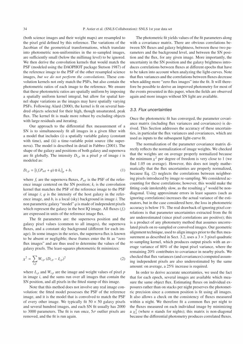
SNLS-04D3fk

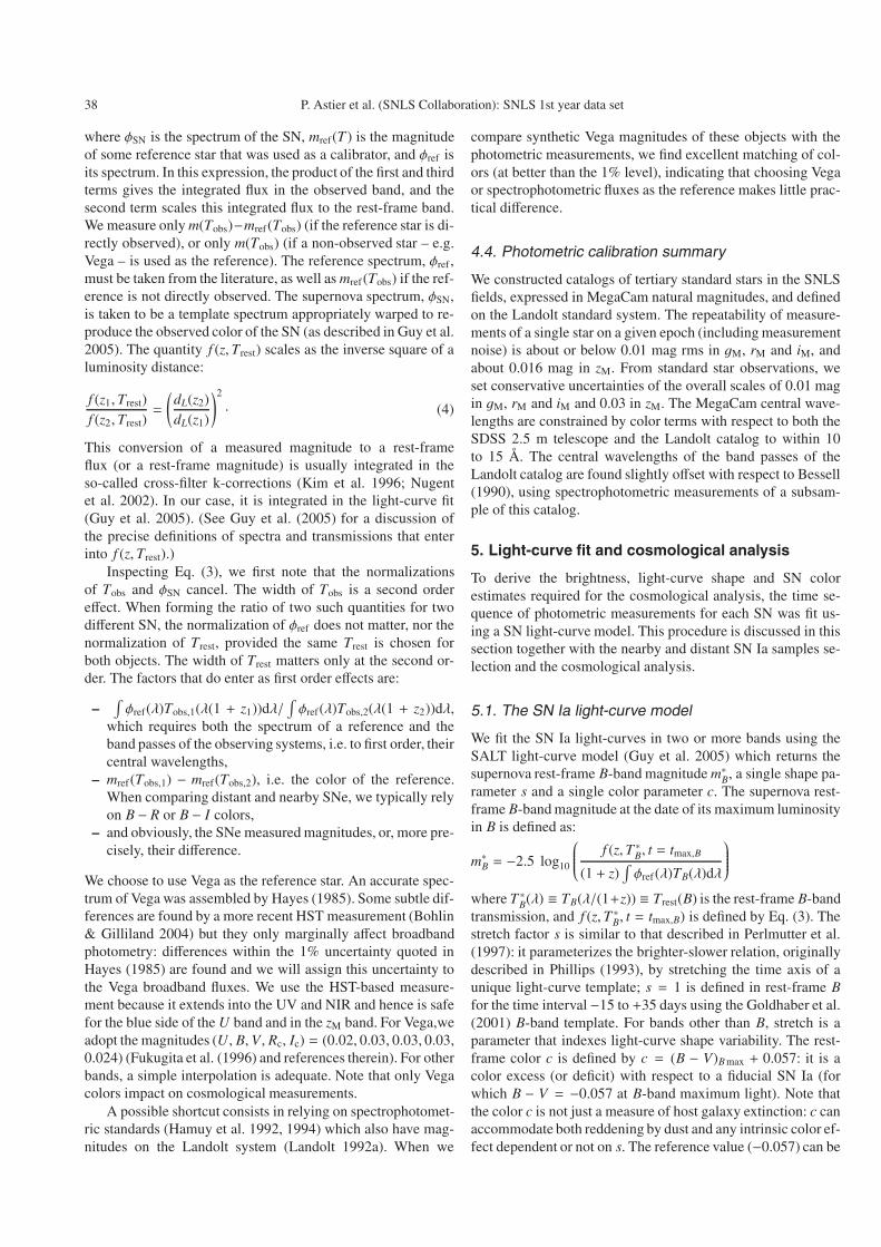
Fig. 1. Observed light-curves points of the SN Ia SNLS-04D3fkin gM, rM, iM and zM bands, along with the multi-color light-curvemodel (described in Sect. 5.1). Note the regular sampling of the ob-servations both before and after maximum light. With a SN redshiftof 0.358, the four measured pass-bands lie in the wavelength rangeof the light-curve model, defined by rest-frame U to R bands, andall light-curves points are therefore fitted simultaneously with onlyfour free parameters (photometric normalization, date of maximum, astretch and a color parameter).

The χ2n contribution of every individual image is evaluated, and

outliers>5σ (due to, for example, unidentified cosmic rays) arediscarded; this cut eliminates 1.4% of the measurements on av-erage. The covariance of the per-night fluxes is then extracted,and normalized so that the minimum χ2

n per degree of free-dom is 1. This translates into an “effective” flux uncertaintyderived from the scatter of repeated observations rather thanfrom first principles. If the only source of noise (beyond photonstatistics) were pixel correlations introduced by image resam-pling, we would expect an average χ2

n/Nd.o.f. of 1.25, as all fluxvariances are on average under-estimated by 25%. Our averagevalue is 1.55; hence we conclude that our photometric uncer-tainties are only ∼12% (

√(1.55/1.25) − 1) larger than photon

statistics, leaving little margin for drastic improvement.Table 2 summarizes the statistics of the differential pho-

tometry fits in each filter. The larger values of χ2n/Nd.o.f. in iM

and zM probably indicate contributions from residual fringes.Examples of SNe Ia light-curves points are presented in Figs. 1and 2 showing SNe at z = 0.358 and z = 0.91 respectively.Also shown on these figures are the results of the light-curvesfits described in Sect. 5.1.

The next section discusses how accurately the SN fluxescan be extracted from the science frames relative to nearbyfield stars, i.e. how well the method assigns magnitudes to SNe,given magnitudes of the field stars which are used for photo-metric calibration, called tertiary standards hereafter.

3.4. Photometric alignment of supernovae relativeto tertiary standards

The SN flux measurement technique of Sect. 3.2 deliversSN fluxes on the same photometric scale as the reference im-age. In this Section, we discuss how we measure ratios of theSN fluxes to those of the tertiary standards (namely stars in the

JD 2450000+3100 3150 3200

Flu

x

Mg

Mi

Mr

Mz

0

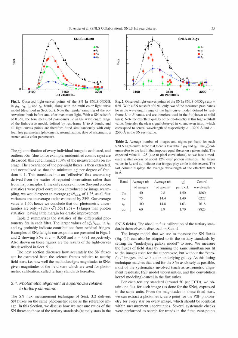
SNLS-04D3gx

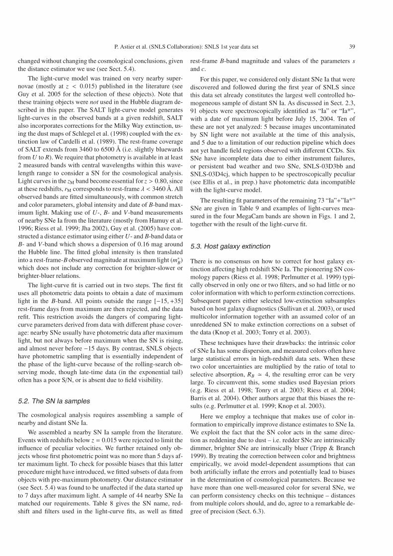
Fig. 2. Observed light-curves points of the SN Ia SNLS-04D3gx at z =0.91. With a SN redshift of 0.91, only two of the measured pass-bandslie in the wavelength range of the light-curve model, defined by rest-frame U to R bands, and are therefore used in the fit (shown as solidlines). Note the excellent quality of the photometry at this high redshiftvalue. Note also the clear signal observed in rM and even in gM, whichcorrespond to central wavelength of respectively λ ∼ 3200 Å and λ ∼2500 Å in the SN rest-frame.

Table 2. Average number of images and nights per band for eachSNLS light-curve. Note that there is less data in gM and zM. The χ2

n col-umn refers to the last fit that imposes equal fluxes on a given night. Theexpected value is 1.25 (due to pixel correlations), so we face a mod-erate scatter excess of about 12% over photon statistics. The largervalues in iM and zM indicate that fringes play a role in this excess. Thelast column displays the average wavelength of the effective filtersin Å.

Band Average nb. Average nb. χ2n Central

of images of epochs per d.o.f. wavelength

gM 40 9.8 1.50 4860

rM 75 14.4 1.40 6227

iM 100 14.8 1.63 7618

zM 60 7.9 1.70 8823

SNLS fields). The absolute flux calibration of the tertiary stan-dards themselves is discussed in Sect. 4.

The image model that we use to measure the SN fluxes(Eq. (1)) can also be adapted to fit the tertiary standards bysetting the “underlying galaxy model” to zero. We measurethe fluxes of field stars by running the same simultaneous fitto the images used for the supernovae, but without the “zero-flux” images, and without an underlying galaxy. As this fittingtechnique matches that used for the SNe as closely as possible,most of the systematics involved (such as astrometric align-ment residuals, PSF model uncertainties, and the convolutionkernel modeling) cancel in the flux ratios.

For each tertiary standard (around 50 per CCD), we ob-tain one flux for each image (as done for the SNe), expressedin the same units. From the magnitudes of these fitted stars,we can extract a photometric zero point for the PSF photom-etry for every star on every image, which should be identicalwithin measurement uncertainties. Several systematic checkswere performed to search for trends in the fitted zero-points

36 P. Astier et al. (SNLS Collaboration): SNLS 1st year data set

as a function of several variables (including image number,star magnitude, and star color); no significant trends were de-tected. As zero-points are obtained from single measurementson single images, the individual measurements are both numer-ous and noisy, with a typical rms of 0.03 mag; however sincethey have the same expectation value, we averaged them usinga robust fit to the distribution peak to obtain a single zero-pointper observed filter.

To test how accurately the ratio of SN flux to tertiary stan-dard stars is retrieved by our technique, we tested the methodon simulated SNe. For each artificial supernova, we selected arandom host galaxy, a neighboring bright star (the model star),and a down-scale ratio (r). For half of the images that enter thefit, we superimposed a scaled-down copy (by a factor r) of themodel on the host galaxy. We rounded the artificial position atan integer pixel offset from the model star to avoid re-sampling.We then performed the full SN fit (i.e. one that allows for anunderlying galaxy model and “zero flux images”) at the posi-tion of the artificial object, and performed the calibration starfit (i.e. one with no galaxy mode and no “zero-flux images”) atthe original position of the model star. This matches exactly thetechnique used for the measurement and calibration of a realSN. We then compared the recovered flux ratio to the (known)down-scale ratio.

We found no significant bias as a function of SN flux orgalaxy brightness at the level of 1%, except at signal-to-noise(S/N) ratios (integrated over the whole light-curve) below 10.At a S/N ratio of 10, fluxes are on average underestimated byless than 1%; this bias rises to about 3% at a S/N ratio of 7.This small flux bias disappears when the fitted object position isfixed, as expected because the fit is then linear. For this reason,when fitting zM light-curves of objects at z > 0.7, for which theS/N is expected to be low, we use the fixed SN position fromthat obtained from the iM and rM fits.

Given the statistics of our simulations, the systematic un-certainty of SN fluxes due to the photometric method employedis less than 1% across the range of S/N we encounter in realdata, and the observed scatter of the retrieved “fake SNe” fluxesbehaves in the same way as that for real SNe. Over a limitedrange of S/N (more than 100 integrated over the whole light-curve), we can exclude biases at the 0.002 mag level. Our upperlimits for a flux bias have a negligible impact on the cosmologi-cal conclusions drawn from the sample described here, and willlikely be improved with further detailed simulations.

4. Photometric calibration

The supernova light-curves produced by the techniques de-scribed in Sect. 3.2 are calibrated relative to nearby field stars(the tertiary standards). Our next step is to place these instru-mental fluxes onto a photometric calibration system using ob-servations of stars of known magnitudes.

4.1. Photometric calibration of tertiary standards

Several standard star calibration catalogs are available inthe literature, such as the Landolt (1983, 1992b) Johnson-Cousins (Vega-based) UBVRI system, or the Smith et al. (2002)

u′g′r′i′z′ AB-magnitude system which is used to calibrate theSloan Digital Sky Survey (SDSS). However, there are sys-tematic errors affecting the transformations between the Smithet al. (2002) system and the widely used Landolt system. Asdiscussed in Fukugita et al. (1996), these errors arise from var-ious sources, for example uncertainties in the cross-calibrationof the spectral energy distributions of the AB fundamental stan-dard stars relative to that of Vega. Since the nearby SNe used inour cosmological fits were extracted from the literature and aretypically calibrated using the standard star catalogs of Landolt(1992b), we adopted the same calibration source for our high-redshift sample. This avoids introducing additional systematicuncertainties between the distant and nearby SN fluxes, whichare used to determine the cosmological parameters. To elim-inate uncertainties associated with color corrections, we de-rive magnitudes in the natural MegaCam filter system.

Both standard and science fields were repeatedly observedover a period of about 18 months. Photometric nights wereselected using the CFHT “Skyprobe” instrument (Cuillandre2003), which monitors atmospheric transparency in the direc-tion that the telescope is pointing. Only the 50% of nightswith the smallest scatter in transparency were considered. Foreach night, stars were selected in the science fields and theiraperture fluxes measured and corrected to an airmass of 1 us-ing the average atmospheric extinction of Mauna Kea. Theseaperture fluxes were then averaged, allowing for photometricratios between exposures. Stable observing conditions wereindicated by a very small scatter in these photometric ratios(typically 0.2%); again the averaging was robust, with 5-σdeviations rejected. Observations of the Landolt standard starfields were processed in the same manner, though their fluxeswere not averaged. The apertures were chosen sufficiently large(about 6′′ in diameter) to bring the variations of aperture cor-rections across the mosaic below 0.005 mag. However, sincefluxes are measured in the same way and in the same aperturesin science images and standard star fields, we did not apply anyaperture correction.

Using standard star observations, we first determined zero-points by fitting linear color transformations and zero-points toeach night and filter, however with color slopes common to allnights. In order to account for possible non-linearities in theLandolt to MegaCam color relations, the observed color−colorrelations were then compared to synthetic ones derived fromspectrophotometric standards. This led to shifts of roughly 0.01in all bands other than gM, for which the shift was 0.03 due tothe nontrivial relation to B and V .

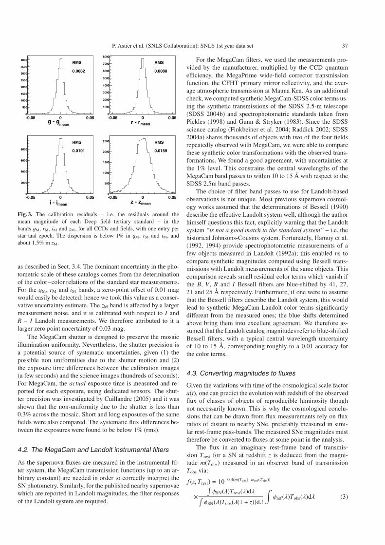
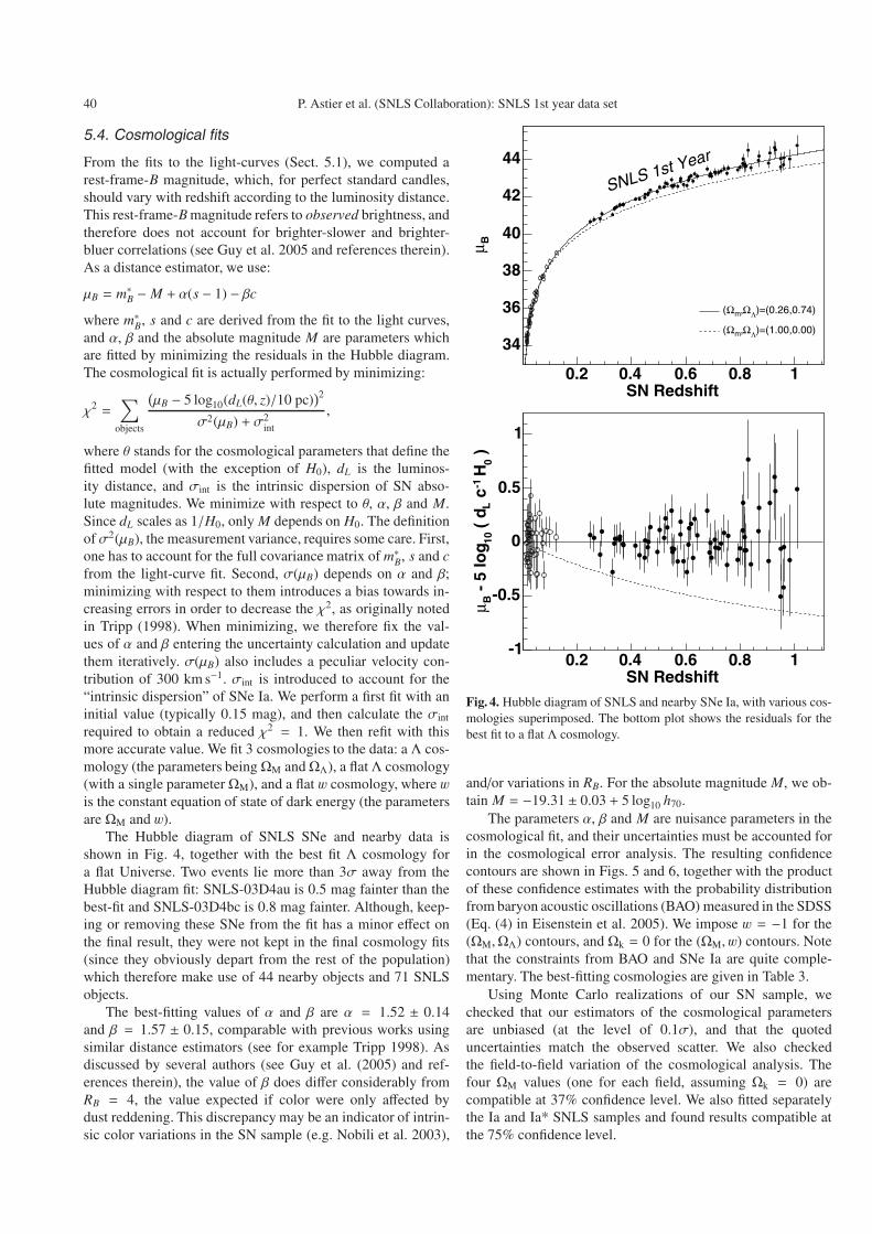
We then applied the zero-points appropriate for each nightto the catalog of science field stars of that same night.These magnitudes were averaged robustly, rejecting 5-σ out-liers, and the average standard star observations were merged.Figure 3 shows the dispersion of the calibration residuals inthe gM, rM, iM and zM bands. The observed standard deviation,which sets the upper bound to the repeatability of the photo-metric measurements, is about or below 0.01 mag in gM, rM

and iM, and about 0.016 mag in zM.For each of the four SNLS fields, a catalog of tertiary

standards was produced using the procedure described above.These catalogs were then used to calibrate the supernova fluxes,

P. Astier et al. (SNLS Collaboration): SNLS 1st year data set 37

mean

g - g-0.05 0 0.050

500

1000

1500

2000

2500

3000

3500

4000RMS

0.0082

meanr - r-0.05 0 0.050

1000

2000

3000

4000

5000

6000

7000

8000

RMS

0.0088

meani - i-0.05 0 0.050

2000

4000

6000

8000

RMS

0.0101

meanz - z-0.05 0 0.050

500

1000

1500

2000

2500 RMS

0.0159

Fig. 3. The calibration residuals – i.e. the residuals around themean magnitude of each Deep field tertiary standard – in thebands gM, rM, iM and zM, for all CCDs and fields, with one entry perstar and epoch. The dispersion is below 1% in gM, rM and iM, andabout 1.5% in zM.

as described in Sect. 3.4. The dominant uncertainty in the pho-tometric scale of these catalogs comes from the determinationof the color−color relations of the standard star measurements.For the gM, rM and iM bands, a zero-point offset of 0.01 magwould easily be detected; hence we took this value as a conser-vative uncertainty estimate. The zM band is affected by a largermeasurement noise, and it is calibrated with respect to I andR − I Landolt measurements. We therefore attributed to it alarger zero point uncertainty of 0.03 mag.

The MegaCam shutter is designed to preserve the mosaicillumination uniformity. Nevertheless, the shutter precision isa potential source of systematic uncertainties, given (1) thepossible non uniformities due to the shutter motion and (2)the exposure time differences between the calibration images(a few seconds) and the science images (hundreds of seconds).For MegaCam, the actual exposure time is measured and re-ported for each exposure, using dedicated sensors. The shut-ter precision was investigated by Cuillandre (2005) and it wasshown that the non-uniformity due to the shutter is less than0.3% across the mosaic. Short and long exposures of the samefields were also compared. The systematic flux differences be-tween the exposures were found to be below 1% (rms).

4.2. The MegaCam and Landolt instrumental filters

As the supernova fluxes are measured in the instrumental fil-ter system, the MegaCam transmission functions (up to an ar-bitrary constant) are needed in order to correctly interpret theSN photometry. Similarly, for the published nearby supernovaewhich are reported in Landolt magnitudes, the filter responsesof the Landolt system are required.

For the MegaCam filters, we used the measurements pro-vided by the manufacturer, multiplied by the CCD quantumefficiency, the MegaPrime wide-field corrector transmissionfunction, the CFHT primary mirror reflectivity, and the aver-age atmospheric transmission at Mauna Kea. As an additionalcheck, we computed synthetic MegaCam-SDSS color terms us-ing the synthetic transmissions of the SDSS 2.5-m telescope(SDSS 2004b) and spectrophotometric standards taken fromPickles (1998) and Gunn & Stryker (1983). Since the SDSSscience catalog (Finkbeiner et al. 2004; Raddick 2002; SDSS2004a) shares thousands of objects with two of the four fieldsrepeatedly observed with MegaCam, we were able to comparethese synthetic color transformations with the observed trans-formations. We found a good agreement, with uncertainties atthe 1% level. This constrains the central wavelengths of theMegaCam band passes to within 10 to 15 Å with respect to theSDSS 2.5m band passes.

The choice of filter band passes to use for Landolt-basedobservations is not unique. Most previous supernova cosmol-ogy works assumed that the determinations of Bessell (1990)describe the effective Landolt system well, although the authorhimself questions this fact, explicitly warning that the Landoltsystem “is not a good match to the standard system” – i.e. thehistorical Johnsons-Cousins system. Fortunately, Hamuy et al.(1992, 1994) provide spectrophotometric measurements of afew objects measured in Landolt (1992a); this enabled us tocompare synthetic magnitudes computed using Bessell trans-missions with Landolt measurements of the same objects. Thiscomparison reveals small residual color terms which vanish ifthe B, V , R and I Bessell filters are blue-shifted by 41, 27,21 and 25 Å respectively. Furthermore, if one were to assumethat the Bessell filters describe the Landolt system, this wouldlead to synthetic MegaCam-Landolt color terms significantlydifferent from the measured ones; the blue shifts determinedabove bring them into excellent agreement. We therefore as-sumed that the Landolt catalog magnitudes refer to blue-shiftedBessell filters, with a typical central wavelength uncertaintyof 10 to 15 Å, corresponding roughly to a 0.01 accuracy forthe color terms.

4.3. Converting magnitudes to fluxes

Given the variations with time of the cosmological scale factora(t), one can predict the evolution with redshift of the observedflux of classes of objects of reproducible luminosity thoughnot necessarily known. This is why the cosmological conclu-sions that can be drawn from flux measurements rely on fluxratios of distant to nearby SNe, preferably measured in simi-lar rest-frame pass-bands. The measured SNe magnitudes musttherefore be converted to fluxes at some point in the analysis.

The flux in an imaginary rest-frame band of transmis-sion Trest for a SN at redshift z is deduced from the magni-tude m(Tobs) measured in an observer band of transmissionTobs via:

f (z, Trest) = 10−0.4(m(Tobs)−mref (Tobs))

×∫φSN(λ)Trest(λ)dλ∫

φSN(λ)Tobs(λ(1 + z))dλ

∫φref(λ)Tobs(λ)dλ (3)

38 P. Astier et al. (SNLS Collaboration): SNLS 1st year data set

where φSN is the spectrum of the SN, mref(T ) is the magnitudeof some reference star that was used as a calibrator, and φref isits spectrum. In this expression, the product of the first and thirdterms gives the integrated flux in the observed band, and thesecond term scales this integrated flux to the rest-frame band.We measure only m(Tobs)−mref (Tobs) (if the reference star is di-rectly observed), or only m(Tobs) (if a non-observed star – e.g.Vega – is used as the reference). The reference spectrum, φref ,must be taken from the literature, as well as mref (Tobs) if the ref-erence is not directly observed. The supernova spectrum, φSN,is taken to be a template spectrum appropriately warped to re-produce the observed color of the SN (as described in Guy et al.2005). The quantity f (z, Trest) scales as the inverse square of aluminosity distance:

f (z1, Trest)f (z2, Trest)

=

(dL(z2)dL(z1)

)2

· (4)

This conversion of a measured magnitude to a rest-frameflux (or a rest-frame magnitude) is usually integrated in theso-called cross-filter k-corrections (Kim et al. 1996; Nugentet al. 2002). In our case, it is integrated in the light-curve fit(Guy et al. 2005). (See Guy et al. (2005) for a discussion ofthe precise definitions of spectra and transmissions that enterinto f (z, Trest).)

Inspecting Eq. (3), we first note that the normalizationsof Tobs and φSN cancel. The width of Tobs is a second ordereffect. When forming the ratio of two such quantities for twodifferent SN, the normalization of φref does not matter, nor thenormalization of Trest, provided the same Trest is chosen forboth objects. The width of Trest matters only at the second or-der. The factors that do enter as first order effects are:

–∫φref(λ)Tobs,1(λ(1 + z1))dλ/

∫φref(λ)Tobs,2(λ(1 + z2))dλ,

which requires both the spectrum of a reference and theband passes of the observing systems, i.e. to first order, theircentral wavelengths,

– mref (Tobs,1) − mref (Tobs,2), i.e. the color of the reference.When comparing distant and nearby SNe, we typically relyon B − R or B − I colors,

– and obviously, the SNe measured magnitudes, or, more pre-cisely, their difference.

We choose to use Vega as the reference star. An accurate spec-trum of Vega was assembled by Hayes (1985). Some subtle dif-ferences are found by a more recent HST measurement (Bohlin& Gilliland 2004) but they only marginally affect broadbandphotometry: differences within the 1% uncertainty quoted inHayes (1985) are found and we will assign this uncertainty tothe Vega broadband fluxes. We use the HST-based measure-ment because it extends into the UV and NIR and hence is safefor the blue side of the U band and in the zM band. For Vega,weadopt the magnitudes (U, B, V , Rc, Ic) = (0.02, 0.03, 0.03, 0.03,0.024) (Fukugita et al. (1996) and references therein). For otherbands, a simple interpolation is adequate. Note that only Vegacolors impact on cosmological measurements.

A possible shortcut consists in relying on spectrophotomet-ric standards (Hamuy et al. 1992, 1994) which also have mag-nitudes on the Landolt system (Landolt 1992a). When we

compare synthetic Vega magnitudes of these objects with thephotometric measurements, we find excellent matching of col-ors (at better than the 1% level), indicating that choosing Vegaor spectrophotometric fluxes as the reference makes little prac-tical difference.

4.4. Photometric calibration summary

We constructed catalogs of tertiary standard stars in the SNLSfields, expressed in MegaCam natural magnitudes, and definedon the Landolt standard system. The repeatability of measure-ments of a single star on a given epoch (including measurementnoise) is about or below 0.01 mag rms in gM, rM and iM, andabout 0.016 mag in zM. From standard star observations, weset conservative uncertainties of the overall scales of 0.01 magin gM, rM and iM and 0.03 in zM. The MegaCam central wave-lengths are constrained by color terms with respect to both theSDSS 2.5 m telescope and the Landolt catalog to within 10to 15 Å. The central wavelengths of the band passes of theLandolt catalog are found slightly offset with respect to Bessell(1990), using spectrophotometric measurements of a subsam-ple of this catalog.

5. Light-curve fit and cosmological analysis

To derive the brightness, light-curve shape and SN colorestimates required for the cosmological analysis, the time se-quence of photometric measurements for each SN was fit us-ing a SN light-curve model. This procedure is discussed in thissection together with the nearby and distant SN Ia samples se-lection and the cosmological analysis.

5.1. The SN Ia light-curve model

We fit the SN Ia light-curves in two or more bands using theSALT light-curve model (Guy et al. 2005) which returns thesupernova rest-frame B-band magnitude m∗B, a single shape pa-rameter s and a single color parameter c. The supernova rest-frame B-band magnitude at the date of its maximum luminosityin B is defined as:

m∗B = −2.5 log10

⎛⎜⎜⎜⎜⎜⎝ f (z, T ∗B, t = tmax,B

(1 + z)∫φref (λ)TB(λ)dλ

⎞⎟⎟⎟⎟⎟⎠where T ∗B(λ) ≡ TB(λ/(1+z)) ≡ Trest(B) is the rest-frame B-bandtransmission, and f (z, T ∗B, t = tmax,B) is defined by Eq. (3). Thestretch factor s is similar to that described in Perlmutter et al.(1997): it parameterizes the brighter-slower relation, originallydescribed in Phillips (1993), by stretching the time axis of aunique light-curve template; s = 1 is defined in rest-frame Bfor the time interval −15 to +35 days using the Goldhaber et al.(2001) B-band template. For bands other than B, stretch is aparameter that indexes light-curve shape variability. The rest-frame color c is defined by c = (B − V)B max + 0.057: it is acolor excess (or deficit) with respect to a fiducial SN Ia (forwhich B − V = −0.057 at B-band maximum light). Note thatthe color c is not just a measure of host galaxy extinction: c canaccommodate both reddening by dust and any intrinsic color ef-fect dependent or not on s. The reference value (−0.057) can be

P. Astier et al. (SNLS Collaboration): SNLS 1st year data set 39

changed without changing the cosmological conclusions, giventhe distance estimator we use (see Sect. 5.4).

The light-curve model was trained on very nearby super-novae (mostly at z < 0.015) published in the literature (seeGuy et al. 2005 for the selection of these objects). Note thatthese training objects were not used in the Hubble diagram de-scribed in this paper. The SALT light-curve model generateslight-curves in the observed bands at a given redshift, SALTalso incorporates corrections for the Milky Way extinction, us-ing the dust maps of Schlegel et al. (1998) coupled with the ex-tinction law of Cardelli et al. (1989). The rest-frame coverageof SALT extends from 3460 to 6500 Å (i.e. slightly bluewardsfrom U to R). We require that photometry is available in at least2 measured bands with central wavelengths within this wave-length range to consider a SN for the cosmological analysis.Light curves in the zM band become essential for z > 0.80, sinceat these redshifts, rM corresponds to rest-frame λ < 3460 Å. Allobserved bands are fitted simultaneously, with common stretchand color parameters, global intensity and date of B-band max-imum light. Making use of U-, B- and V-band measurementsof nearby SNe Ia from the literature (mostly from Hamuy et al.1996; Riess et al. 1999; Jha 2002), Guy et al. (2005) have con-structed a distance estimator using either U- and B-band data orB- and V-band which shows a dispersion of 0.16 mag aroundthe Hubble line. The fitted global intensity is then translatedinto a rest-frame-B observed magnitude at maximum light (m∗B)which does not include any correction for brighter-slower orbrighter-bluer relations.

The light-curve fit is carried out in two steps. The first fituses all photometric data points to obtain a date of maximumlight in the B-band. All points outside the range [−15,+35]rest-frame days from maximum are then rejected, and the datarefit. This restriction avoids the dangers of comparing light-curve parameters derived from data with different phase cover-age: nearby SNe usually have photometric data after maximumlight, but not always before maximum when the SN is rising,and almost never before −15 days. By contrast, SNLS objectshave photometric sampling that is essentially independent ofthe phase of the light-curve because of the rolling-search ob-serving mode, though late-time data (in the exponential tail)often has a poor S/N, or is absent due to field visibility.

5.2. The SN Ia samples

The cosmological analysis requires assembling a sample ofnearby and distant SNe Ia.

We assembled a nearby SN Ia sample from the literature.Events with redshifts below z = 0.015 were rejected to limit theinfluence of peculiar velocities. We further retained only ob-jects whose first photometric point was no more than 5 days af-ter maximum light. To check for possible biases that this latterprocedure might have introduced, we fitted subsets of data fromobjects with pre-maximum photometry. Our distance estimator(see Sect. 5.4) was found to be unaffected if the data started upto 7 days after maximum light. A sample of 44 nearby SNe Iamatched our requirements. Table 8 gives the SN name, red-shift and filters used in the light-curve fits, as well as fitted

rest-frame B-band magnitude and values of the parameters sand c.

For this paper, we considered only distant SNe Ia that werediscovered and followed during the first year of SNLS sincethis data set already constitutes the largest well controlled ho-mogeneous sample of distant SN Ia. As discussed in Sect. 2.3,91 objects were spectroscopically identified as “Ia” or “Ia*”,with a date of maximum light before July 15, 2004. Ten ofthese are not yet analyzed: 5 because images uncontaminatedby SN light were not available at the time of this analysis,and 5 due to a limitation of our reduction pipeline which doesnot yet handle field regions observed with different CCDs. SixSNe have incomplete data due to either instrument failures,or persistent bad weather and two SNe, SNLS-03D3bb andSNLS-03D4cj, which happen to be spectroscopically peculiar(see Ellis et al., in prep.) have photometric data incompatiblewith the light-curve model.

The resulting fit parameters of the remaining 73 “Ia”+”Ia*”SNe are given in Table 9 and examples of light-curves mea-sured in the four MegaCam bands are shown in Figs. 1 and 2,together with the result of the light-curve fit.

5.3. Host galaxy extinction

There is no consensus on how to correct for host galaxy ex-tinction affecting high redshift SNe Ia. The pioneering SN cos-mology papers (Riess et al. 1998; Perlmutter et al. 1999) typi-cally observed in only one or two filters, and so had little or nocolor information with which to perform extinction corrections.Subsequent papers either selected low-extinction subsamplesbased on host galaxy diagnostics (Sullivan et al. 2003), or usedmulticolor information together with an assumed color of anunreddened SN to make extinction corrections on a subset ofthe data (Knop et al. 2003; Tonry et al. 2003).

These techniques have their drawbacks: the intrinsic colorof SNe Ia has some dispersion, and measured colors often havelarge statistical errors in high-redshift data sets. When thesetwo color uncertainties are multiplied by the ratio of total toselective absorption, RB 4, the resulting error can be verylarge. To circumvent this, some studies used Bayesian priors(e.g. Riess et al. 1998; Tonry et al. 2003; Riess et al. 2004;Barris et al. 2004). Other authors argue that this biases the re-sults (e.g. Perlmutter et al. 1999; Knop et al. 2003).

Here we employ a technique that makes use of color in-formation to empirically improve distance estimates to SNe Ia.We exploit the fact that the SN color acts in the same direc-tion as reddening due to dust – i.e. redder SNe are intrinsicallydimmer, brighter SNe are intrinsically bluer (Tripp & Branch1999). By treating the correction between color and brightnessempirically, we avoid model-dependent assumptions that canboth artificially inflate the errors and potentially lead to biasesin the determination of cosmological parameters. Because wehave more than one well-measured color for several SNe, wecan perform consistency checks on this technique – distancesfrom multiple colors should, and do, agree to a remarkable de-gree of precision (Sect. 6.3).

40 P. Astier et al. (SNLS Collaboration): SNLS 1st year data set

5.4. Cosmological fits

From the fits to the light-curves (Sect. 5.1), we computed arest-frame-B magnitude, which, for perfect standard candles,should vary with redshift according to the luminosity distance.This rest-frame-B magnitude refers to observed brightness, andtherefore does not account for brighter-slower and brighter-bluer correlations (see Guy et al. 2005 and references therein).As a distance estimator, we use:

µB = m∗B − M + α(s − 1) − βcwhere m∗B, s and c are derived from the fit to the light curves,and α, β and the absolute magnitude M are parameters whichare fitted by minimizing the residuals in the Hubble diagram.The cosmological fit is actually performed by minimizing:

χ2 =∑

objects

(µB − 5 log10(dL(θ, z)/10 pc)

)2

σ2(µB) + σ2int

,

where θ stands for the cosmological parameters that define thefitted model (with the exception of H0), dL is the luminos-ity distance, and σint is the intrinsic dispersion of SN abso-lute magnitudes. We minimize with respect to θ, α, β and M.Since dL scales as 1/H0, only M depends on H0. The definitionof σ2(µB), the measurement variance, requires some care. First,one has to account for the full covariance matrix of m∗B, s and cfrom the light-curve fit. Second, σ(µB) depends on α and β;minimizing with respect to them introduces a bias towards in-creasing errors in order to decrease the χ2, as originally notedin Tripp (1998). When minimizing, we therefore fix the val-ues of α and β entering the uncertainty calculation and updatethem iteratively. σ(µB) also includes a peculiar velocity con-tribution of 300 km s−1. σint is introduced to account for the“intrinsic dispersion” of SNe Ia. We perform a first fit with aninitial value (typically 0.15 mag), and then calculate the σint

required to obtain a reduced χ2 = 1. We then refit with thismore accurate value. We fit 3 cosmologies to the data: a Λ cos-mology (the parameters beingΩM andΩΛ), a flatΛ cosmology(with a single parameter ΩM), and a flat w cosmology, where wis the constant equation of state of dark energy (the parametersare ΩM and w).

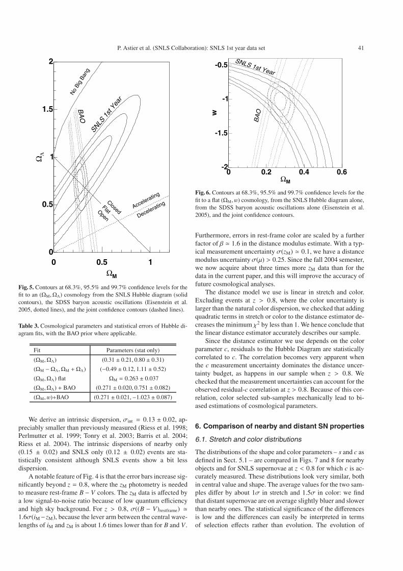
The Hubble diagram of SNLS SNe and nearby data isshown in Fig. 4, together with the best fit Λ cosmology fora flat Universe. Two events lie more than 3σ away from theHubble diagram fit: SNLS-03D4au is 0.5 mag fainter than thebest-fit and SNLS-03D4bc is 0.8 mag fainter. Although, keep-ing or removing these SNe from the fit has a minor effect onthe final result, they were not kept in the final cosmology fits(since they obviously depart from the rest of the population)which therefore make use of 44 nearby objects and 71 SNLSobjects.

The best-fitting values of α and β are α = 1.52 ± 0.14and β = 1.57 ± 0.15, comparable with previous works usingsimilar distance estimators (see for example Tripp 1998). Asdiscussed by several authors (see Guy et al. (2005) and ref-erences therein), the value of β does differ considerably fromRB = 4, the value expected if color were only affected bydust reddening. This discrepancy may be an indicator of intrin-sic color variations in the SN sample (e.g. Nobili et al. 2003),

SN Redshift0.2 0.4 0.6 0.8 1

Bµ

34

36

38

40

42

44

)=(0.26,0.74)ΛΩ,mΩ(

)=(1.00,0.00)ΛΩ,mΩ(

SNLS 1st Year

SN Redshift0.2 0.4 0.6 0.8 1

) 0 H

-1 c

L (

d10

- 5

log

Bµ

-1

-0.5

0

0.5

1

Fig. 4. Hubble diagram of SNLS and nearby SNe Ia, with various cos-mologies superimposed. The bottom plot shows the residuals for thebest fit to a flat Λ cosmology.

and/or variations in RB. For the absolute magnitude M, we ob-tain M = −19.31 ± 0.03 + 5 log10 h70.

The parameters α, β and M are nuisance parameters in thecosmological fit, and their uncertainties must be accounted forin the cosmological error analysis. The resulting confidencecontours are shown in Figs. 5 and 6, together with the productof these confidence estimates with the probability distributionfrom baryon acoustic oscillations (BAO) measured in the SDSS(Eq. (4) in Eisenstein et al. 2005). We impose w = −1 for the(ΩM,ΩΛ) contours, and Ωk = 0 for the (ΩM, w) contours. Notethat the constraints from BAO and SNe Ia are quite comple-mentary. The best-fitting cosmologies are given in Table 3.

Using Monte Carlo realizations of our SN sample, wechecked that our estimators of the cosmological parametersare unbiased (at the level of 0.1σ), and that the quoteduncertainties match the observed scatter. We also checkedthe field-to-field variation of the cosmological analysis. Thefour ΩM values (one for each field, assuming Ωk = 0) arecompatible at 37% confidence level. We also fitted separatelythe Ia and Ia* SNLS samples and found results compatible atthe 75% confidence level.

P. Astier et al. (SNLS Collaboration): SNLS 1st year data set 41

MΩ0 0.5 1

ΛΩ

0

0.5

1

1.5

2

SNLS 1

st Y

ear

BA

O

ClosedFlatOpen

Accelerating

Decelerating

No

Big

Bang

Fig. 5. Contours at 68.3%, 95.5% and 99.7% confidence levels for thefit to an (ΩM,ΩΛ) cosmology from the SNLS Hubble diagram (solidcontours), the SDSS baryon acoustic oscillations (Eisenstein et al.2005, dotted lines), and the joint confidence contours (dashed lines).

Table 3. Cosmological parameters and statistical errors of Hubble di-agram fits, with the BAO prior where applicable.

Fit Parameters (stat only)

(ΩM,ΩΛ) (0.31 ± 0.21, 0.80 ± 0.31)

(ΩM − ΩΛ,ΩM + ΩΛ) (−0.49 ± 0.12, 1.11 ± 0.52)

(ΩM,ΩΛ) flat ΩM = 0.263 ± 0.037

(ΩM,ΩΛ) + BAO (0.271 ± 0.020, 0.751 ± 0.082)

(ΩM, w)+BAO (0.271 ± 0.021,−1.023 ± 0.087)

We derive an intrinsic dispersion, σint = 0.13 ± 0.02, ap-preciably smaller than previously measured (Riess et al. 1998;Perlmutter et al. 1999; Tonry et al. 2003; Barris et al. 2004;Riess et al. 2004). The intrinsic dispersions of nearby only(0.15 ± 0.02) and SNLS only (0.12 ± 0.02) events are sta-tistically consistent although SNLS events show a bit lessdispersion.

A notable feature of Fig. 4 is that the error bars increase sig-nificantly beyond z = 0.8, where the zM photometry is neededto measure rest-frame B − V colors. The zM data is affected bya low signal-to-noise ratio because of low quantum efficiencyand high sky background. For z > 0.8, σ((B − V)restframe) 1.6σ(iM−zM), because the lever arm between the central wave-lengths of iM and zM is about 1.6 times lower than for B and V .

MΩ0 0.2 0.4 0.6

w

-2

-1.5

-1

-0.5SNLS 1st Year

BA

O

Fig. 6. Contours at 68.3%, 95.5% and 99.7% confidence levels for thefit to a flat (ΩM, w) cosmology, from the SNLS Hubble diagram alone,from the SDSS baryon acoustic oscillations alone (Eisenstein et al.2005), and the joint confidence contours.

Furthermore, errors in rest-frame color are scaled by a furtherfactor of β 1.6 in the distance modulus estimate. With a typ-ical measurement uncertainty σ(zM) 0.1, we have a distancemodulus uncertaintyσ(µ) > 0.25. Since the fall 2004 semester,we now acquire about three times more zM data than for thedata in the current paper, and this will improve the accuracy offuture cosmological analyses.

The distance model we use is linear in stretch and color.Excluding events at z > 0.8, where the color uncertainty islarger than the natural color dispersion, we checked that addingquadratic terms in stretch or color to the distance estimator de-creases the minimum χ2 by less than 1. We hence conclude thatthe linear distance estimator accurately describes our sample.

Since the distance estimator we use depends on the colorparameter c, residuals to the Hubble Diagram are statisticallycorrelated to c. The correlation becomes very apparent whenthe c measurement uncertainty dominates the distance uncer-tainty budget, as happens in our sample when z > 0.8. Wechecked that the measurement uncertainties can account for theobserved residual-c correlation at z > 0.8. Because of this cor-relation, color selected sub-samples mechanically lead to bi-ased estimations of cosmological parameters.

6. Comparison of nearby and distant SN properties

6.1. Stretch and color distributions

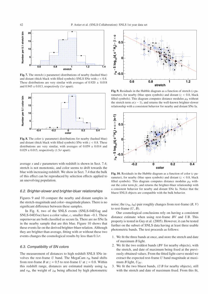
The distributions of the shape and color parameters – s and c asdefined in Sect. 5.1 – are compared in Figs. 7 and 8 for nearbyobjects and for SNLS supernovae at z < 0.8 for which c is ac-curately measured. These distributions look very similar, bothin central value and shape. The average values for the two sam-ples differ by about 1σ in stretch and 1.5σ in color: we findthat distant supernovae are on average slightly bluer and slowerthan nearby ones. The statistical significance of the differencesis low and the differences can easily be interpreted in termsof selection effects rather than evolution. The evolution of

42 P. Astier et al. (SNLS Collaboration): SNLS 1st year data set

stretch0.6 0.8 1 1.2 1.4

Nu

mb

er p

er 0

.1 s

tret

ch b

in

0

5

10

15

20

Fig. 7. The stretch (s parameter) distributions of nearby (hashed blue)and distant (thick black with filled symbols) SNLS SNe with z < 0.8.These distributions are very similar with averages of 0.920 ± 0.018and 0.945 ± 0.013, respectively (1σ apart).

color-0.4 -0.2 0 0.2 0.4

Nu

mb

er p

er 0

.1 c

olo

r b

in

0

5

10

15

20

Fig. 8. The color (c parameter) distributions for nearby (hashed blue)and distant (thick black with filled symbols) SNe with z < 0.8. Thesedistributions are very similar, with averages of 0.059 ± 0.014 and0.029 ± 0.015, respectively (1.5σ apart).

average s and c parameters with redshift is shown in Sect. 7.4;stretch is not monotonic, and color seems to drift towards theblue with increasing redshift. We show in Sect. 7.4 that the bulkof this effect can be reproduced by selection effects applied toan unevolving population.

6.2. Brighter-slower and brighter-bluer relationships

Figures 9 and 10 compare the nearby and distant samples inthe stretch-magnitude and color−magnitude planes. There is nosignificant difference between these samples.

In Fig. 8, two of the SNLS events (SNLS-04D1ag andSNLS-04D3oe) have a color value, c, smaller than −0.1. Thesesupernovae are both classified as secure Ia. There are no SNe Iain the nearby sample that are this blue. Figure 10 shows thatthese events lie on the derived brighter-bluer relation. Althoughthey are brighter than average, fitting with or without these twoevents changes the cosmological results by less than 0.1σ.

6.3. Compatibility of SN colors

The measurement of distances to high redshift SNLS SNe in-volves the rest-frame U band. The MegaCam rM band shiftsfrom rest-frame B at z = 0.5 to rest-frame U at z = 0.8.Withinthis redshift range, distances are estimated mainly using iMand rM, the weight of zM being affected by high photometric

stretch0.6 0.8 1 1.2

c× β)

- 0

H-1

c l(d

10 -

5 lo

gBµ -0.5

0

0.5

Fig. 9. Residuals in the Hubble diagram as a function of stretch (s pa-rameter), for nearby (blue open symbols) and distant (z < 0.8, blackfilled symbols). This diagram computes distance modulus µB withoutthe stretch term α(s − 1), and returns the well-known brighter-slowerrelationship with a consistent behavior for nearby and distant SNe Ia.

color-0.2 0 0.2 0.4

(s-

1)× α

) +

0 H

-1 c l

(d10

- 5

log

Bµ

-0.5

0

0.5

Fig. 10. Residuals in the Hubble diagram as a function of color (c pa-rameter), for nearby (blue open symbols) and distant (z < 0.8, blackfilled symbols). This diagram computes distance modulus µB with-out the color term βc, and returns the brighter-bluer relationship witha consistent behavior for nearby and distant SNe Ia. Notice that thebluest SNLS objects are compatible with the bulk behavior.

noise; the (rM, iM) pair roughly changes from rest-frame (B, V)to rest-frame (U, B).

Our cosmological conclusions rely on having a consistentdistance estimate when using rest-frame BV and UB. Thisproperty is tested in Guy et al. (2005). However, it can be testedfurther on the subset of SNLS data having at least three usablephotometric bands. The test proceeds as follows:

1. We fit the three bands at once, and store the stretch and dateof maximum B light.

2. We fit the two reddest bands (BV for nearby objects), withthe stretch, and date of maximum being fixed at the previ-ously obtained values. From the fitted light-curve model weextract the expected rest-frame U band magnitude at maxi-mum B light, UBV .

3. We fit the two bluest bands, (UB for nearby objects), stillwith the stretch and date of maximum fixed. From this fit,

P. Astier et al. (SNLS Collaboration): SNLS 1st year data set 43

SN Redshift0 0.2 0.4 0.6 0.8

3 U∆

-0.5

0

0.5

Fig. 11. ∆U3, difference between rest-frame U peak magnitude “pre-dicted” from B and V , and the measured value, as a function of red-shift. The error bars reflect photometric uncertainties. The redshift re-gions have been chosen so that the measured bands roughly sample theUBV rest-frame region. The differences between average values forthe three samples agree within statistical uncertainties, indicating thatthe relation between U, B and V brightnesses does not change withredshift. Although the nearby and intermediate samples have compa-rable photometric resolution, the intermediate sample exhibits a farsmaller scatter. We attribute this difference to the practical difficultiesin calibrating U band observations.

we extract the expected rest-frame U band magnitude atmaximum B light. Since it matches the measurement whenthe actual U flux is measured, we call it Umeas.

The test quantity is ∆U3 ≡ UBV − Umeas, i.e. the “predicted” U(derived from B and V) minus the measured U brightness.Forcing both quantities to be measured with the same stretchand B maximum date is not essential, but narrows the distri-bution of residuals. A residual of zero means that the threemeasured bands agree with the light-curve model for a cer-tain parameter set, and hence that the distance estimate willbe identical for the two different color fits.

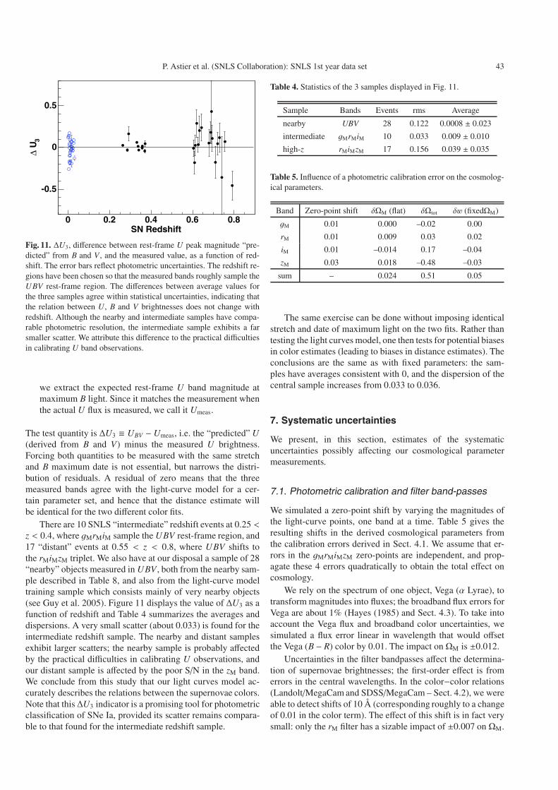
There are 10 SNLS “intermediate” redshift events at 0.25 <z < 0.4, where gMrMiM sample the UBV rest-frame region, and17 “distant” events at 0.55 < z < 0.8, where UBV shifts tothe rMiMzM triplet. We also have at our disposal a sample of 28“nearby” objects measured in UBV , both from the nearby sam-ple described in Table 8, and also from the light-curve modeltraining sample which consists mainly of very nearby objects(see Guy et al. 2005). Figure 11 displays the value of ∆U3 as afunction of redshift and Table 4 summarizes the averages anddispersions. A very small scatter (about 0.033) is found for theintermediate redshift sample. The nearby and distant samplesexhibit larger scatters; the nearby sample is probably affectedby the practical difficulties in calibrating U observations, andour distant sample is affected by the poor S/N in the zM band.We conclude from this study that our light curves model ac-curately describes the relations between the supernovae colors.Note that this ∆U3 indicator is a promising tool for photometricclassification of SNe Ia, provided its scatter remains compara-ble to that found for the intermediate redshift sample.

Table 4. Statistics of the 3 samples displayed in Fig. 11.

Sample Bands Events rms Average

nearby UBV 28 0.122 0.0008 ± 0.023

intermediate gMrMiM 10 0.033 0.009 ± 0.010

high-z rMiMzM 17 0.156 0.039 ± 0.035

Table 5. Influence of a photometric calibration error on the cosmolog-ical parameters.

Band Zero-point shift δΩM (flat) δΩtot δw (fixedΩM)

gM 0.01 0.000 –0.02 0.00

rM 0.01 0.009 0.03 0.02

iM 0.01 –0.014 0.17 –0.04

zM 0.03 0.018 –0.48 –0.03

sum – 0.024 0.51 0.05

The same exercise can be done without imposing identicalstretch and date of maximum light on the two fits. Rather thantesting the light curves model, one then tests for potential biasesin color estimates (leading to biases in distance estimates). Theconclusions are the same as with fixed parameters: the sam-ples have averages consistent with 0, and the dispersion of thecentral sample increases from 0.033 to 0.036.

7. Systematic uncertainties

We present, in this section, estimates of the systematicuncertainties possibly affecting our cosmological parametermeasurements.

7.1. Photometric calibration and filter band-passes

We simulated a zero-point shift by varying the magnitudes ofthe light-curve points, one band at a time. Table 5 gives theresulting shifts in the derived cosmological parameters fromthe calibration errors derived in Sect. 4.1. We assume that er-rors in the gMrMiMzM zero-points are independent, and prop-agate these 4 errors quadratically to obtain the total effect oncosmology.

We rely on the spectrum of one object, Vega (α Lyrae), totransform magnitudes into fluxes; the broadband flux errors forVega are about 1% (Hayes (1985) and Sect. 4.3). To take intoaccount the Vega flux and broadband color uncertainties, wesimulated a flux error linear in wavelength that would offsetthe Vega (B − R) color by 0.01. The impact on ΩM is ±0.012.

Uncertainties in the filter bandpasses affect the determina-tion of supernovae brightnesses; the first-order effect is fromerrors in the central wavelengths. In the color−color relations(Landolt/MegaCam and SDSS/MegaCam – Sect. 4.2), we wereable to detect shifts of 10 Å (corresponding roughly to a changeof 0.01 in the color term). The effect of this shift is in fact verysmall: only the rM filter has a sizable impact of ±0.007 on ΩM.

44 P. Astier et al. (SNLS Collaboration): SNLS 1st year data set

7.2. Light-curve fitting, (U – B) color and k-corrections

If the light-curve model fails to properly describe the true light-curve shape, the result would be a bias in the light-curve param-eters, and possibly in the cosmological parameters if the biasdepends on redshift. We have already discussed two possiblecauses of such a bias: the influence of the first measurementdate (Sect. 5.2), and the choice of rest-frame bands used tomeasure brightness and color (Sect. 6.3). Both have very smalleffects. However, given only 10 intermediate redshift SNLSevents, each with an uncertainty of 0.033, the precision withwhich we can define the average (U − B) color at given (B−V)is limited to about 0.01 mag by our sample size.

Uncertainties in the k-corrections (due to SNe Ia spectralvariability at fixed color) contribute directly to the observedscatter. The redshift range of the intermediate redshift sam-ple of Sect. 6.3 corresponds to a rest-frame wavelength spanof about 400 Å, in a region where SNe Ia spectra are highlystructured. Since we observe compatible intrinsic dispersionsfor nearby and SNLS events (indeed, slightly lower for SNLS),we find no evidence that k-correction uncertainties add signifi-cantly to the intrinsic dispersion.

Nevertheless, since the measured scatter of the intermediateredshift sample appears surprisingly small and, since the sam-ple size is small, we used a more conservative value of 0.02for the light-curve model error, to account for both the errors inthe colors and from k-corrections. A shift of the U-band light-curve model of 0.02 mag results in a change in ΩM of 0.018.This is to be added to the statistical uncertainty.

7.3. U-band variability and evolution of SNe Ia

Concerns have been expressed regarding the use of rest-frameU-band fluxes to measure luminosity distances (e.g. Jha 2002and Nugent et al. 2002), motivated by the apparent large vari-ability of the U-band luminosity of SNe Ia. Such variabilityseems also to be present at intermediate redshifts althoughthere seems to be little obvious evolution to z = 0.5 of the over-all UV SED (Ellis et al., in prep.). Note that Guy et al. (2005)have succeeded in constructing a distance estimator using U-and B-band data which shows a dispersion of only 0.16 magaround the Hubble line, comparable to that found for distancesderived using B- and V-band data. Note also that the quan-tity ∆U3 appears to be independent of redshift, implying thatif the average luminosity of SNe Ia evolves with redshift, thisevolution must preserve the UBV rest-frame color relations.Lentz et al. (2000) predict a strong dependence of the UV fluxfrom the progenitor metallicity (at fixed B − V color), whichshould have been visible if metallicity evolution were indeedpresent.

7.4. Malmquist bias

The Malmquist bias may affect the cosmological conclusionsby altering the average brightness of measured SNe in a red-shift dependent way. The mechanism is however not exactlystraightforward since the reconstructed distance depends on

stretch and color, and not only on the brightness. We haveconducted simulations, both of nearby SN searches and of theSNLS survey, to investigate the effects on the derivation of cos-mological parameters.

We simulated light-curves of nearby SNe Ia (0.02 < z <0.1) with random explosion date, stretch and color, using theobserved brighter-slower and brighter-bluer correlations. Wethen simulated a brightness cut at a fixed date. Although thenumber of “detected” events and their average redshift stronglydepends on the brightness cut, the average distance bias of thesurvivors is found to change by less than 10%, when varyingboth the value and the sharpness of the brightness cut. The biasis also essentially independent of the discovery phase, althoughthe peak brightness is not. We find a distance modulus biasof 0.027 (similar in B, V and R), sensitive at the 10% level tothe unknown details of nearby searches. Note that the redshiftdependence of the distance bias of the nearby sample has noimpact on the cosmological measurements: only the averagebias matters.

The crude simulation we conducted applies only to fluxlimited searches, which applies to about half of the sample.We compute an average bias value for our nearby sample asthe simulation result (0.027 mag) times the fraction of eventsto which it applies. Assuming that both factors suffer from anuncertainty of 50%, we find an average nearby sample biasvalue of 0.017 ± 0.012 mag. A global increase of all nearbydistances by 0.017(±0.012) mag increases ΩM (flat universe)by 0.019 (±0.013).

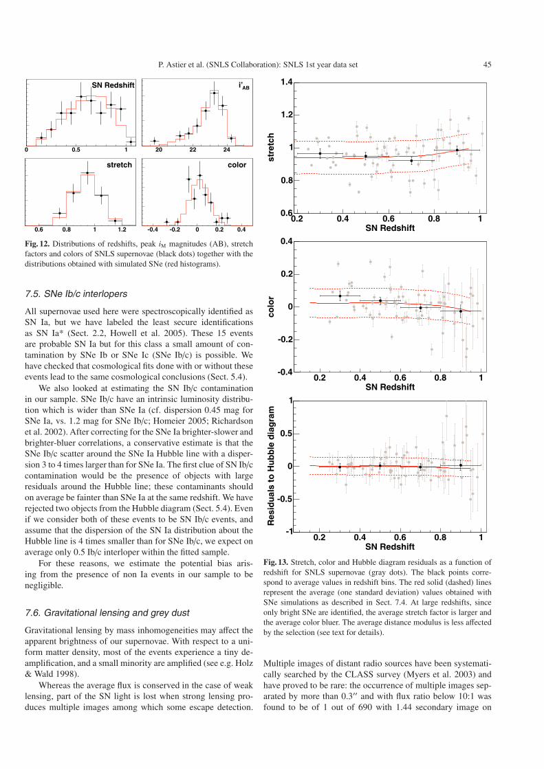
For the distant SNLS sample, which is flux limited, we sim-ulated supernovae at a rate per co-moving volume independentof redshift, accounted for the brighter-slower and brighter-bluercorrelations, and adjusted the position and smoothness of thelimiting magnitude cut in order to reproduce the redshift andpeak magnitude distributions. In contrast with nearby SN sim-ulations, here we have many observed distributions for a singlesearch, and the key parameters that enter the simulation arehighly constrained. The best match to SNLS data is shown inFig. 12, and Fig. 13 shows the expected biases as a functionof redshift in the shape and color parameters, and for our dis-tance estimator. The distance modulus bias is about 0.02 magat z = 0.8, increasing to 0.05 at z = 1. Correcting for the com-puted bias decreases ΩM (flat Universe) by 0.02. We assumedthat the uncertainty in this bias correction is 50% of its value.

To summarize: we find that the differential bias betweennearby and distant samples almost exactly cancels, and esti-mate an overall uncertainty of 0.016 in ΩM (flat Universe).Since applying the Malmquist bias corrections changes the cos-mological results by less than 0.1σ, the corrections have notbeen applied. However, in the future, when the SNLS sam-ple size increases, modeling and applying the Malmquist biascorrection will assume a greater importance. The same ap-plies to the nearby sample, where having a more controlledand homogeneous sample, discovered by a single search (e.g.SN Factory, Aldering et al. 2002) will be essential to reduce theassociated systematic uncertainty.

P. Astier et al. (SNLS Collaboration): SNLS 1st year data set 45

0 0.5 1

SN Redshift

20 22 24

ABi’

0.6 0.8 1 1.2

stretch

-0.4 -0.2 0 0.2 0.4

color

Fig. 12. Distributions of redshifts, peak iM magnitudes (AB), stretchfactors and colors of SNLS supernovae (black dots) together with thedistributions obtained with simulated SNe (red histograms).

7.5. SNe Ib/c interlopers

All supernovae used here were spectroscopically identified asSN Ia, but we have labeled the least secure identificationsas SN Ia* (Sect. 2.2, Howell et al. 2005). These 15 eventsare probable SN Ia but for this class a small amount of con-tamination by SNe Ib or SNe Ic (SNe Ib/c) is possible. Wehave checked that cosmological fits done with or without theseevents lead to the same cosmological conclusions (Sect. 5.4).

We also looked at estimating the SN Ib/c contaminationin our sample. SNe Ib/c have an intrinsic luminosity distribu-tion which is wider than SNe Ia (cf. dispersion 0.45 mag forSNe Ia, vs. 1.2 mag for SNe Ib/c; Homeier 2005; Richardsonet al. 2002). After correcting for the SNe Ia brighter-slower andbrighter-bluer correlations, a conservative estimate is that theSNe Ib/c scatter around the SNe Ia Hubble line with a disper-sion 3 to 4 times larger than for SNe Ia. The first clue of SN Ib/ccontamination would be the presence of objects with largeresiduals around the Hubble line; these contaminants shouldon average be fainter than SNe Ia at the same redshift. We haverejected two objects from the Hubble diagram (Sect. 5.4). Evenif we consider both of these events to be SN Ib/c events, andassume that the dispersion of the SN Ia distribution about theHubble line is 4 times smaller than for SNe Ib/c, we expect onaverage only 0.5 Ib/c interloper within the fitted sample.

For these reasons, we estimate the potential bias aris-ing from the presence of non Ia events in our sample to benegligible.

7.6. Gravitational lensing and grey dust

Gravitational lensing by mass inhomogeneities may affect theapparent brightness of our supernovae. With respect to a uni-form matter density, most of the events experience a tiny de-amplification, and a small minority are amplified (see e.g. Holz& Wald 1998).

Whereas the average flux is conserved in the case of weaklensing, part of the SN light is lost when strong lensing pro-duces multiple images among which some escape detection.

SN Redshift0.2 0.4 0.6 0.8 1

stre

tch

0.6

0.8

1

1.2

1.4

SN Redshift0.2 0.4 0.6 0.8 1

colo

r

-0.4

-0.2

0

0.2

0.4

SN Redshift0.2 0.4 0.6 0.8 1

Res

idu

als

to H

ub

ble

dia

gra

m

-1

-0.5

0

0.5

1

Fig. 13. Stretch, color and Hubble diagram residuals as a function ofredshift for SNLS supernovae (gray dots). The black points corre-spond to average values in redshift bins. The red solid (dashed) linesrepresent the average (one standard deviation) values obtained withSNe simulations as described in Sect. 7.4. At large redshifts, sinceonly bright SNe are identified, the average stretch factor is larger andthe average color bluer. The average distance modulus is less affectedby the selection (see text for details).

Multiple images of distant radio sources have been systemati-cally searched by the CLASS survey (Myers et al. 2003) andhave proved to be rare: the occurrence of multiple images sep-arated by more than 0.3′′ and with flux ratio below 10:1 wasfound to be of 1 out of 690 with 1.44 secondary image on

46 P. Astier et al. (SNLS Collaboration): SNLS 1st year data set

average, with inefficiencies due to the separation and flux ra-tio cuts of 13% and 37% respectively (Browne et al. 2003).Multiple images with a smaller separation are not resolved inthe SNLS, and their time delay is much smaller than the typi-cal duration of a SN light curve2 so that no flux is lost for suchevents. Hence CLASS results provide us with an upper limitfor the number of (resolved) strong lensing cases in the SNLSsupernova sample, given the fact that CLASS sources are glob-ally more distant (see Chae 2003). Assuming (pessimistically)that for each strongly lensed SN, we see only one image, theflux bias is smaller than 0.3% at z = 1.

Gravitational lensing also broadens asymmetrically thebrightness distribution of SNe at large redshifts (Bergströmet al. 2000). As a consequence, a cosmological fit usingSNe magnitudes (instead of fluxes) is biased. Holz & Linder(2004) found a dispersion of 0.088 × z (note that Bergströmet al. 2000 find a value of ∼0.04 at z = 1 for smooth haloprofiles in flat ΛCDM), which translates into a bias of the aver-age magnitude of ∼0.004× z. The broadening of the brightnessdistribution also affects the cosmological parameters uncertain-ties. In the cosmological fit, we have derived a constant “intrin-sic” dispersion which includes the average dispersion due tolensing. Neglecting its redshift dependence has no significantimpact on the accuracy of the errors derived for the cosmolog-ical parameters.

In summary, the total effect of lensing on cosmological pa-rameters is very small. We find that ΩM for a flat ΛCDM cos-mology and the equation of state for a flat universe withBAO constraints, are shifted by at most −0.005 and −0.01 re-spectively. We therefore did not apply any correction to ourresults.

The possibility that SNe Ia could be dimmed by intergalac-tic grey dust (i.e. with weak extinction variation over the opticalwavelengths) has been suggested by Aguirre (1999a,b) as anastrophysical alternative to the dark energy hypothesis. Somesimple dust scenarios without a cosmological constant couldbe excluded by Riess et al. (2004) using SNe Ia data. Studyingthe colors of a large sample of quasars, Östman & Mörtsell(2005) were able to set limits on the light absorption length asa function of RV , but these limits can only be translated into anupper bound of supernovae dimming. Conservatively assumingRV = 12, using the SNOC program (Goobar et al. 2002), wecomputed an upper limit in the dimming of supernovae whichtranslates into a shift of −0.025 inΩM for aΛCDM cosmology,and a shift of −0.048 in w for a flat cosmology with constantequation of state when combined with SDSS BAO results. Notethat these are upper limits and that a scenario without any in-tergalactic dust cannot be excluded. We therefore did not applyany correction to our results.

8. Summary and perspectives

Table 6 summarizes the uncertainties affecting our cosmolog-ical parameter measurements. The table includes the impact

2 Delays are of order of a day for a source at z = 1 and a point-likelens at z = 0.5 for a typical angular separation of 0.2′′ (Bergströmet al. 2000).

Table 6. Summary of uncertainties in the derived cosmological param-eters. The dominant systematic uncertainty arises from the photomet-ric calibration, itself dominated by the iM and zM band contributions.

Source σ(ΩM) σ(Ωtot) σ(w) σ(ΩM) σ(w)

(flat) (with BAO)

Zero-points 0.024 0.51 0.05 0.004 0.040

Vega spectrum 0.012 0.02 0.03 0.003 0.024

Filter bandpasses 0.007 0.01 0.02 0.002 0.013

Malmquist bias 0.016 0.22 0.03 0.004 0.025

Sum (sys) 0.032 0.55 0.07 0.007 0.054

Meas. errors 0.037 0.52 0.09 0.020 0.087

U − B color (stat) 0.020 0.10 0.05 0.003 0.021

Sum (stat) 0.042 0.53 0.10 0.021 0.090

of uncertainties in several parameter directions: the ΩM di-rection for a flat (ΩM,ΩΛ) (i.e. w = −1) cosmology, the Ωtot

direction for a general (ΩM,ΩΛ) cosmology, and the w direc-tion at fixed ΩM for a (ΩM, w) cosmology. We also report herethe observed shifts when the BAO prior is applied to a flat(ΩM, w) cosmology. Note that measurement and isolation ofsystematic errors is a major goal of the SNLS. Some of theseuncertainties will decrease as more data is acquired and futurepapers will examine a wider range of issues, using our growingdataset.

Combining Tables 3 and 6, we obtain the following results:

ΩM = 0.263 ± 0.042 (stat) ± 0.032 (syst)

for a flat Λ cosmology, and

ΩM = 0.271 ± 0.021 (stat) ± 0.007 (syst)

w = −1.023 ± 0.090 (stat) ± 0.054 (syst)

w < −0.85 (95% CL)

for a flat cosmology with constant equation of state, whenour constraints are combined with the BAO SDSS results.Assuming w > −1 brings our upper limit to −0.83 (at 95% CL).Supernovae alone give a marginal constraint: w < −0.5at 95% CL.

These results agree well with previous works, both fromSNe Ia, and also from other sources. For example Seljak et al.(2005) finds very similar results combining CMB, LSS andLyα constraints. The dominant systematic uncertainties arisefrom the nearby sample and from the photometric calibrationof the zM band; both will be improved in the future. The multi-band light-curves allow us to study color relations as a functionof redshift; these data are expected to be sensitive indicators ofevolution. We observed a surprisingly narrow correlation be-tween (U−B) and (B−V) (using the ∆U3 indicator), indicatingthat the dispersion in U-band properties is well correlated withmeasurements in redder bands.

From the first year of SNLS data, we placed 71 distantevents on the Hubble Diagram, with 10 more from the sameperiod to be added later. (Our full first year statistics wouldhave been around 100 SNe Ia with spectroscopic confirma-tion had we not lost Feb. 2004 to an instrument failure.) Our

P. Astier et al. (SNLS Collaboration): SNLS 1st year data set 47

time sampling, filter coverage, and image quality have now sig-nificantly improved since early 2004, and we now regularlyacquire 2−3 times as much data in zM. A precise photomet-ric calibration is essential, and we are now working with theCFHTLS community in refining the photometric calibrationof the MegaCam instrument. We have embarked on the pro-cess of calibrating tertiary standards in our fields, from Sloansecondary and primary standards. This will allow us to cross-check the Vega/Landolt zero-points, and more accurately cali-brate zM band observations.

After only two years of operation, the SNLS has alreadydemonstrated its advantages over all previous ground-basedsupernova surveys. The “rolling search” technique is robustto weather and instrument-related problems, and the techni-cal characteristics of the survey are now well understood.The average rate of spectroscopically-confirmed SNe Ia iscurrently about 10 per lunation and continues to increase. Upuntil July 2005, the SNLS sample includes more than 200 spec-troscopically identified SNe Ia, most with excellent photomet-ric temporal and filter coverage. An extrapolation of the cur-rent rate to the end of the survey indicates that we should reachour goal of building a Hubble diagram with about 700 spectro-scopically identified well-measured SN Ia events. The SNLSalready has the largest-ever sample of high-z SNe discoveredby a single telescope, and will eventually produce a homoge-neous, high-quality sample that is an order of magnitude largerstill.

High statistical accuracy benefits the control of systemat-ics. With our unmatched SN statistics, by year 5 we will beable to populate each ∼0.1 redshift bin with ∼100 SNe Ia, thusfilling the brightness, decline-rate, and color 3-dimensional pa-rameter space. This will enable us to detect possible driftsin “SNe Ia demographics”, and control Malmquist bias.Moreover, the rolling-search observing mode produces manyevents at low to intermediate redshift with superb photometricaccuracy, because integration times are tailored for the faintestobjects. These relatively bright events permit demanding inter-nal consistency tests, and may lead to improvements in distanceestimation.

Acknowledgements. The authors wish to recognize and acknowl-edge the very significant cultural role and reverence that the sum-mit of Mauna Kea has always had within the indigenous Hawaiiancommunity. We are most fortunate to have the opportunity to con-duct observations from this mountain. We gratefully acknowledgethe assistance of the CFHT Queued Service Observing Team, ledby P. Martin (CFHT). We heavily rely on the dedication of theCFHT staff and particularly J.-C. Cuillandre for continuous im-provement of the instrument performance. The real-time pipelinesfor supernovae detection run on computers integrated in the CFHTcomputing system, and are very efficiently installed, maintainedand monitored by K. Withington (CFHT). We also heavily rely onthe real-time Elixir pipeline which is operated and monitored byJ-C. Cuillandre, E. Magnier and K. Withington. We are grateful toL. Simard (CADC) for setting up the image delivery system andhis kind and efficient responses to our suggestions for improve-ments. The French collaboration members carry out the data reduc-tions using the CCIN2P3. Canadian collaboration members acknowl-edge support from NSERC and CIAR; French collaboration mem-bers from CNRS/IN2P3, CNRS/INSU, PNC and CEA. This work

was supported in part by the Director, Office of Science, Office ofHigh Energy and Nuclear Physics, of the US Department of Energy.The France-Berkeley Fund provided additional collaboration sup-port. CENTRA members were supported by Fundação para a Ciênciae Tecnologia (FCT), Portugal under POCTI/FNU/43423. S. Fabbroand C. Gonçalves acknowledge support from FCT under grants noSFRH/BPD/14682/2003 and SFRH/BPD/11641/2002 respectively.

References

Aguirre, A. 1999a, ApJ, 525, 583Aguirre, A. N. 1999b, ApJ, 512, L19Alard, C. 2000, A&AS, 144, 363Alard, C., & Lupton, R. H. 1998, ApJ, 503, 325Aldering, G., Adam, G., Antilogus, P., et al. 2002, in Survey and Other

Telescope Technologies and Discoveries, ed. T. J. Anthony, & W.Sidney, Proc. SPIE, 4836, 61

Altavilla, G., et al. 2004, MNRAS, 349, 1344Barris, B. J., Tonry, J. L., Blondin, S., et al. 2004, ApJ, 602, 571Basa, S., Astier, P., & Aubourg, E. 2005, in preparationBergström, L., Goliath, M., Goobar, A., & Mörtsell, E. 2000, A&A,

358, 13Bertin, E., & Arnouts, S. 1996, A&AS, 117, 393Bessell, M. S. 1990, PASP, 102, 1181Bohlin, R. C., & Gilliland, R. L. 2004, AJ, 127, 3508Boulade, O., Charlot, X., Abbon, P., et al. 2003, in Instrument Design

and Performance for Optical/Infrared Ground-based Telescopes,ed. Iye, Masanori; Moorwood, Alan F. M., Proc. SPIE, 4841, 72

Browne, I. W. A., Wilkinson, P. N., Jackson, N. J. F., et al. 2003,MNRAS, 341, 13

Cardelli, J. A., Clayton, G. C., & Mathis, J. S. 1989, APJ, 345, 245CFHTLS. 2002, http://cfht.hawaii.edu/Science/CFHTLS,

Tech. rep.Chae, K.-H. 2003, MNRAS, 346, 746Cuillandre, J.-C. 2003, SkyProbe at CFHT: Atmospheric Attenuation,http://www.cfht.hawaii.edu/Instruments/Elixir/skyprobe/

Cuillandre, J.-C. 2005, Shutter ballistics and exposure time,http://cfht.hawaii.edu/Instruments/Imaging/MegaPrime

Eisenstein, D. J., Zehavi, I., Hogg, D. W., et al. 2005, ApJ, 633, 560Ellis, R., Sullivan, M., & Howell, D. 2005, in preparationFabbro, S. 2001, Ph.D. Thesis, Université Denis Diderot, ParisFinkbeiner, D. P., Padmanabhan, N., Schlegel, D. J., et al. 2004, AJ,

128, 2577Fukugita, M., Ichikawa, T., Gunn, J. E., et al. 1996, AJ, 111, 1748Goldhaber, G., Groom, D. E., Kim, A., et al. 2001, ApJ, 558, 359Goobar, A., Mörtsell, E., Amanullah, R., et al. 2002, A&A, 392, 757Gunn, J. E., & Stryker, L. L. 1983, ApJS, 52, 121Guy, J., Astier, P., Nobili, S., Regnault, N., & Pain, R. 2005, A&A,

443, 781Hamuy, M., Phillips, M. M., Suntzeff, N. B., et al. 1996, AJ, 112, 2408Hamuy, M., Suntzeff, N. B., Heathcote, S. R., et al. 1994, PASP, 106,

566Hamuy, M., Walker, A. R., Suntzeff, N. B., et al. 1992, PASP, 104,

533Hayes, D. S. 1985, in Calibration of Fundamental Stellar Quantities,

IAU Symp., 111, 225Holz, D. E., & Linder, E. V. 2004 [arXiv:astro-ph/0412173]Holz, D. E., & Wald, R. M. 1998, Phys. Rev. D, 58, 063501Homeier, N. L. 2005, ApJ, 620, 12Howell, D. A., Sullivan, M., Perret, K., et al. 2005, ApJ, in pressJha, S. 2002, Ph.D. Thesis, University of Washington

48 P. Astier et al. (SNLS Collaboration): SNLS 1st year data set

Kim, A., Goobar, A., & Perlmutter, S. 1996, PASP, 108, 190Knop, R. A., Aldering, G., Amanullah, R., et al. 2003, ApJ, 598, 102Krisciunas, K., Phillips, M. M., Stubbs, C., et al. 2001, AJ, 122, 1616Krisciunas, K., Phillips, M. M., Suntzeff, N. B., et al. 2004a, AJ, 127,

1664Krisciunas, K., Suntzeff, N. B., Phillips, M. M., et al. 2004b, AJ, 128,

3034Landolt, A. U. 1983, AJ, 88, 439Landolt, A. U. 1992a, AJ, 104, 372Landolt, A. U. 1992b, AJ, 104, 340Lentz, E. J., Baron, E., Branch, D., Hauschildt, P. H., & Nugent, P. E.

2000, ApJ, 530, 966Magnier, E. A., & Cuillandre, J.-C. 2004, PASP, 116, 449Myers, S. T., Jackson, N. J., Browne, I. W. A., et al. 2003, MNRAS,

341, 1Nobili, S., Goobar, A., Knop, R., & Nugent, P. 2003, A&A, 404, 901Nugent, P., Kim, A., & Perlmutter, S. 2002, PASP, 114, 803Östman, L., & Mörtsell, E. 2005, JCAP, 0502, 005Perlmutter, S., Gabi, S., Goldhaber, G., et al. 1997, ApJ, 483, 565Perlmutter, S., Aldering, G., Goldhaber, G., et al. 1999, ApJ, 517, 565Phillips, M. M. 1993, ApJ, 413, L105Pickles, A. J. 1998, pasp, 110, 863Raddick, M. J. 2002, BAAS, 34, 1150Richardson, D., Branch, D., Casebeer, D., et al. 2002, AJ, 123, 745Riess, A. G., Filippenko, A. V., Challis, P., et al. 1998, AJ, 116, 1009Riess, A. G., Kirshner, R. P., Schmidt, B. P., et al. 1999, AJ, 117, 707Riess, A. G., Strolger, L., Tonry, J., et al. 2004, ApJ, 607, 665Schlegel, D. J., Finkbeiner, D. P., & Davis, M. 1998, ApJ, 500, 525SDSS 2004a, Sky Server, SDSS Data Release 3,http://cas.sdss.org/dr3/en/

SDSS 2004b, Sky Server, SDSS Data Release 3, Imaging camera pa-rameters and description,http://www.sdss.org/dr3/instruments/imager/

Seljak, U., Makarov, A., McDonald, P., et al. 2005, Phys. Rev. D, 71,103 515

Smith, J. A., Tucker, D. L., Kent, S., et al. 2002, AJ, 123, 2121Stetson, P. B. 1987, PASP, 99, 191Strolger, L.-G., Smith, R. C., Suntzeff, N. B., et al. 2002, AJ, 124,

2905Sullivan, M., Ellis, R. S., Aldering, G., et al. 2003, MNRAS, 340,

1057

Sullivan, M., Howell, A., Perrett, K., et al. 2005, AJ, in pressTonry, J. L., Schmidt, B. P., Barris, B., et al. 2003, ApJ, 594, 1Tripp, R. 1998, A&A, 331, 815Tripp, R., & Branch, D. 1999, ApJ, 525, 209van Dokkum, P. G. 2001, PASP, 113, 1420

1 LPNHE, CNRS-IN2P3 and Universités Paris VI & VII,4 place Jussieu, 75252 Paris Cedex 05, France; e-mail:astier@in2p3.fr

2 APC, Collège de France, 11 place Marcellin Berthelot, 75005Paris, France

3 DSM/DAPNIA, CEA/Saclay, 91191 Gif-sur-Yvette Cedex, France4 Department of Physics and Astronomy, University of Victoria, PO

Box 3055, Victoria, BC VSW 3P6, Canada5 LAM, CNRS, BP8, Traverse du Siphon, 13376 Marseille Cedex

12, France6 Department of Astronomy and Astrophysics, University of

Toronto, 60 St. George Street, Toronto, ON M5S 3H8, Canada7 CENTRA-Centro M. de Astrofisica and Department of Physics,

IST, Lisbon, Portugal8 CPPM, CNRS-IN2P3 and Université Aix-Marseille II, Case 907,

13288 Marseille Cedex 9, France9 University of Oxford Astrophysics, Denys Wilkinson Building,

Keble Road, Oxford OX1 3RH, UK10 Université de Savoie, 73000 Chambery, France11 LBNL, 1 Cyclotron Rd, Berkeley, CA 94720, USA12 ESO, Alonso de Cordova 3107, Vitacura, Casilla 19001, Santiago

19, Chile13 CRAL, 9 avenue Charles André, 69561 Saint-Genis-Laval cedex,

France14 California Institute of Technology, Pasadena, California, USA15 LUTH, UMR 8102, CNRS and Observatoire de Paris, 92195

Meudon, France16 Department of Physics, Stockholm University, Sweden17 IoA, University of Cambridge, Madingley Road, Cambridge CB3

0EZ, UK18 Department of Physics, University of California Berkeley,

Berkeley, CA 94720, USA

P. Astier et al. (SNLS Collaboration): SNLS 1st year data set, Online Material p 1

Online Material

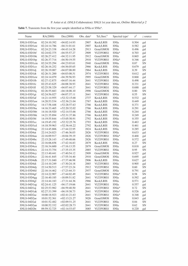
P. Astier et al. (SNLS Collaboration): SNLS 1st year data set, Online Material p 2

Table 7. Transients from the first year sample identified as SNIa or SNIa*.

Name RA(2000) Dec(2000) Obs. datea Tel./Inst.b Spectral typec zd z source

SNLS-03D1au 02:24:10.392 –04:02:14.93 2907 Keck/LRIS SNIa 0.504 galSNLS-03D1aw 02:24:14.786 –04:31:01.61 2907 Keck/LRIS SNIa 0.582 galSNLS-03D1ax 02:24:23.338 –04:43:14.28 2913 Gem/GMOS SNIa 0.496 galSNLS-03D1bf 02:24:02.375 –04:55:57.27 2909 VLT/FORS1 SNIa* 0.703 galSNLS-03D1bk 02:26:27.412 –04:32:11.95 2912 Gem/GMOS SNIa 0.865 galSNLS-03D1bp 02:26:37.714 –04:50:19.55 2910 VLT/FORS1 SNIa* 0.346 galSNLS-03D1cm 02:24:55.294 –04:23:03.61 2940 Gem/GMOS SNIa 0.87 SNSNLS-03D1co 02:26:16.252 –04:56:05.65 2966 Keck/LRIS SNIa 0.679 galSNLS-03D1dj 02:26:19.087 –04:07:08.89 2964 Keck/LRIS SNIa 0.39 SNSNLS-03D1dt 02:26:31.200 –04:03:08.51 2974 VLT/FORS1 SNIa 0.612 galSNLS-03D1ew 02:24:14.079 –04:39:56.93 2995 Gem/GMOS SNIa 0.868 galSNLS-03D1fb 02:27:12.875 –04:07:16.44 2641 VLT/FORS1 SNIa 0.498 galSNLS-03D1fc 02:25:43.625 –04:08:38.93 2641 VLT/FORS1 SNIa 0.331 galSNLS-03D1fl 02:25:58.329 –04:07:44.17 2641 VLT/FORS1 SNIa 0.688 galSNLS-03D1fq 02:26:55.683 –04:18:08.10 2998 Gem/GMOS SNIa 0.80 SNSNLS-03D1gt 02:24:56.027 –04:07:37.11 2641 VLT/FORS1 SNIa 0.55 SNSNLS-03D3af 14:21:14.955 +52:32:15.68 2737 Keck/LRIS SNIa 0.532 galSNLS-03D3aw 14:20:53.534 +52:36:21.04 2767 Keck/LRIS SNIa 0.449 galSNLS-03D3ay 14:17:58.448 +52:28:57.63 2766 Keck/LRIS SNIa 0.371 galSNLS-03D3ba 14:16:33.465 +52:20:32.02 2766 Keck/LRIS SNIa 0.291 galSNLS-03D3bb 14:16:18.920 +52:14:53.66 2766 Keck/LRIS SNIa 0.244 galSNLS-03D3bh 14:21:35.894 +52:31:37.86 2766 Keck/LRIS SNIa 0.249 galSNLS-03D3bl 14:19:55.844 +53:05:50.91 2792 Keck/LRIS SNIa 0.355 galSNLS-03D3cc 14:19:45.192 +52:32:25.76 2793 Keck/LRIS SNIa 0.463 galSNLS-03D3cd 14:18:39.963 +52:36:44.22 2792 Keck/LRIS SNIa 0.461 galSNLS-03D4ag 22:14:45.806 –17:44:22.95 2824 Keck/LRIS SNIa 0.285 galSNLS-03D4at 22:14:24.023 –17:46:36.03 2826 VLT/FORS1 SNIa 0.633 galSNLS-03D4au 22:16:09.917 –18:04:39.19 2826 VLT/FORS1 SNIa* 0.468 galSNLS-03D4bc 22:15:28.143 –17:49:48.66 2826 VLT/FORS1 SNIa 0.572 galSNLS-03D4cj 22:16:06.658 –17:42:16.83 2879 Keck/LRIS SNIa 0.27 SNSNLS-03D4cn 22:16:34.600 –17:16:13.55 2879 Gem/GMOS SNIa 0.818 galSNLS-03D4cx 22:14:33.754 –17:35:15.35 2885 VLT/FORS1 SNIa 0.95 SNSNLS-03D4cy 22:13:40.441 –17:40:54.12 2909 Gem/GMOS SNIa 0.927 galSNLS-03D4cz 22:16:41.845 –17:55:34.40 2910 Gem/GMOS SNIa 0.695 galSNLS-03D4dh 22:17:31.040 –17:37:46.98 2906 Keck/LRIS SNIa 0.627 galSNLS-03D4di 22:14:10.249 –17:30:24.18 2885 VLT/FORS1 SNIa 0.905 galSNLS-03D4dy 22:14:50.513 –17:57:23.24 2912 VLT/FORS1 SNIa 0.60 SNSNLS-03D4fd 22:16:14.462 –17:23:44.33 2937 Gem/GMOS SNIa 0.791 galSNLS-03D4gf 22:14:22.907 –17:44:02.49 2641 VLT/FORS1 SNIa* 0.58 SNSNLS-03D4gg 22:16:40.185 –18:09:51.82 2641 VLT/FORS1 SNIa 0.592 galSNLS-03D4gl 22:14:44.183 –17:31:44.36 2966 Keck/LRIS SNIa 0.571 galSNLS-04D1ag 02:24:41.125 –04:17:19.66 2641 VLT/FORS1 SNIa 0.557 galSNLS-04D1aj 02:25:53.982 –04:59:40.50 2641 VLT/FORS1 SNIa* 0.72 SNSNLS-04D1ak 02:27:33.399 –04:19:38.73 2641 VLT/FORS1 SNIa* 0.526 galSNLS-04D2ac 10:00:18.923 +02:41:21.63 2641 VLT/FORS1 SNIa* 0.348 galSNLS-04D2ae 10:01:52.361 +02:13:21.27 3026 Gem/GMOS SNIa 0.843 galSNLS-04D2al 10:01:52.482 +02:09:51.25 2641 VLT/FORS1 SNIa 0.84 SNSNLS-04D2an 10:00:52.332 +02:02:28.73 2641 VLT/FORS1 SNIa 0.62 SNSNLS-04D2bt 09:59:32.725 +02:14:53.07 3085 VLT/FORS1 SNIa 0.220 gal

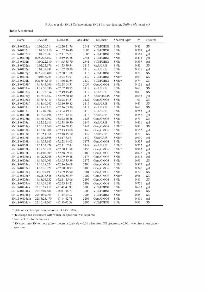
P. Astier et al. (SNLS Collaboration): SNLS 1st year data set, Online Material p 3

Table 7. continued.

Name RA(2000) Dec(2000) Obs. datea Tel./Inst.b Spectral typec zd z source

SNLS-04D2ca 10:01:20.514 +02:20:21.76 2641 VLT/FORS1 SNIa 0.83 SNSNLS-04D2cf 10:01:56.110 +01:52:46.40 3086 VLT/FORS1 SNIa 0.369 galSNLS-04D2cw 10:01:22.787 +02:11:55.31 3085 VLT/FORS1 SNIa 0.568 galSNLS-04D2fp 09:59:28.162 +02:19:15.58 2641 VLT/FORS1 SNIa 0.415 galSNLS-04D2fs 10:00:22.110 +01:45:55.70 2641 VLT/FORS1 SNIa 0.357 galSNLS-04D2gb 10:02:22.676 +01:53:39.34 3117 Keck/LRIS SNIa 0.43 SNSNLS-04D2gc 10:01:39.281 +01:52:59.36 3118 Keck/LRIS SNIa 0.521 galSNLS-04D2gp 09:59:20.400 +02:30:31.88 3116 VLT/FORS1 SNIa 0.71 SNSNLS-04D2iu 10:01:13.221 +02:24:53.91 3139 VLT/FORS1 SNIa* 0.69 SNSNLS-04D2ja 09:58:48.519 +01:46:18.64 3139 VLT/FORS1 SNIa* 0.74 SNSNLS-04D3bf 14:17:45.096 +52:28:04.31 3054 Gem/GMOS SNIa 0.156 galSNLS-04D3co 14:17:50.030 +52:57:48.95 3117 Keck/LRIS SNIa 0.62 SNSNLS-04D3cp 14:20:23.954 +52:49:15.45 3119 Keck/LRIS SNIa 0.83 SNSNLS-04D3cy 14:18:12.452 +52:39:30.40 3115 Keck/DMOS SNIa 0.643 galSNLS-04D3dd 14:17:48.411 +52:28:14.57 3122 Gem/GMOS SNIa 1.01 SNSNLS-04D3df 14:18:10.042 +52:16:39.85 3117 Keck/LRIS SNIa 0.47 SNSNLS-04D3do 14:17:46.113 +52:16:03.36 3117 Keck/LRIS SNIa 0.61 SNSNLS-04D3ez 14:19:07.894 +53:04:19.17 3118 Keck/LRIS SNIa 0.263 galSNLS-04D3fk 14:18:26.198 +52:31:42.74 3118 Keck/LRIS SNIa 0.358 galSNLS-04D3fq 14:16:57.902 +52:22:46.46 3123 Gem/GMOS SNIa 0.73 SNSNLS-04D3gt 14:22:32.611 +52:38:49.30 3149 Keck/LRIS SNIa* 0.451 galSNLS-04D3gx 14:20:13.666 +52:16:58.33 3147 Gem/GMOS SNIa* 0.91 SNSNLS-04D3hn 14:22:06.908 +52:13:43.00 3148 Gem/GMOS SNIa 0.552 galSNLS-04D3is 14:16:51.968 +52:48:45.70 3149 Keck/LRIS SNIa* 0.71 SNSNLS-04D3ki 14:19:34.598 +52:17:32.61 3149 Keck/LRIS SNIa* 0.930 galSNLS-04D3kr 14:16:35.943 +52:28:44.02 3173 Gem/GMOS SNIa 0.337 galSNLS-04D3ks 14:22:33.479 +52:11:07.44 3149 Keck/LRIS SNIa* 0.752 galSNLS-04D3lp 14:19:50.911 +52:30:11.88 3153 Gem/GMOS SNIa* 0.983 galSNLS-04D3lu 14:21:08.009 +52:58:29.74 3180 Gem/GMOS SNIa 0.822 galSNLS-04D3mk 14:19:25.768 +53:09:49.48 3176 Gem/GMOS SNIa 0.813 galSNLS-04D3ml 14:16:39.095 +53:05:35.89 3177 Gem/GMOS SNIa 0.95 SNSNLS-04D3nc 14:16:18.224 +52:16:26.09 3200 Gem/GMOS SNIa* 0.817 galSNLS-04D3nh 14:22:26.729 +52:20:00.92 3180 Gem/GMOS SNIa 0.340 galSNLS-04D3nq 14:20:19.193 +53:09:15.90 3201 Gem/GMOS SNIa 0.22 SNSNLS-04D3nr 14:22:38.526 +52:38:55.89 3202 Gem/GMOS SNIa* 0.96 SNSNLS-04D3ny 14:18:56.332 +52:11:15.06 3197 Gem/GMOS SNIa 0.81 SNSNLS-04D3oe 14:19:39.381 +52:33:14.21 3198 Gem/GMOS SNIa 0.756 galSNLS-04D4an 22:15:57.119 –17:41:43.93 3200 VLT/FORS1 SNIa 0.613 galSNLS-04D4bk 22:15:07.681 –18:03:36.79 3200 VLT/FORS1 SNIa* 0.84 SNSNLS-04D4bq 22:14:49.391 –17:49:39.37 3203 VLT/FORS1 SNIa 0.55 SNSNLS-04D4dm 22:15:25.470 –17:14:42.71 3206 Gem/GMOS SNIa 0.811 galSNLS-04D4dw 22:16:44.667 –17:50:02.38 3206 VLT/FORS1 SNIa 0.96 SN

a Date of spectrocopic observations (JD 2 450 000+).b Telescope and instrument with which the spectrum was acquired.c See Sect. 2.2 for definitions.d SN spectrum (SN) or host galaxy spectrum (gal). δz ∼ 0.01 when from SN spectrum, ∼0.001 when from host galaxy

spectrum.

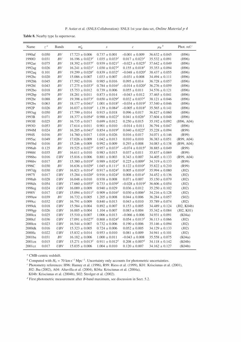
P. Astier et al. (SNLS Collaboration): SNLS 1st year data set, Online Material p 4

Table 8. Nearby type Ia supernovae.

Name z a Bands m∗B s c µBb Phot. ref.c

1990af 0.050 BV 17.723 ± 0.006 0.737 ± 0.001 –0.001 ± 0.009 36.632 ± 0.045 (H96)1990O 0.031 BV 16.196 ± 0.023d 1.035 ± 0.033d 0.017 ± 0.023d 35.532 ± 0.091 (H96)1992ae 0.075 BV 18.392 ± 0.037d 0.939 ± 0.021d –0.023 ± 0.025d 37.642 ± 0.049 (H96)1992ag 0.026 BV 16.241 ± 0.021d 1.030 ± 0.027d 0.155 ± 0.018d 35.353 ± 0.094 (H96)1992aq 0.101 BV 19.299 ± 0.028d 0.839 ± 0.032d –0.048 ± 0.020d 38.437 ± 0.055 (H96)1992bc 0.020 BV 15.086 ± 0.007 1.033 ± 0.007 –0.031 ± 0.008 34.494 ± 0.111 (H96)1992bh 0.045 BV 17.592 ± 0.016 0.985 ± 0.016 0.095 ± 0.014 36.728 ± 0.057 (H96)1992bl 0.043 BV 17.275 ± 0.033d 0.784 ± 0.016d –0.014 ± 0.020d 36.276 ± 0.059 (H96)1992bo 0.018 BV 15.753 ± 0.012 0.739 ± 0.006 0.055 ± 0.011 34.576 ± 0.121 (H96)1992bp 0.079 BV 18.281 ± 0.011 0.873 ± 0.014 –0.043 ± 0.012 37.465 ± 0.041 (H96)1992br 0.088 BV 19.398 ± 0.073d 0.650 ± 0.029d 0.032 ± 0.037d 38.121 ± 0.046 (H96)1992bs 0.063 BV 18.177 ± 0.041d 1.001 ± 0.018d –0.034 ± 0.019d 37.540 ± 0.046 (H96)1992P 0.026 BV 16.037 ± 0.018d 1.139 ± 0.084d –0.005 ± 0.018d 35.565 ± 0.141 (H96)1993ag 0.050 BV 17.799 ± 0.014 0.915 ± 0.018 0.096 ± 0.017 36.827 ± 0.060 (H96)1993B 0.071 BV 18.377 ± 0.054d 0.988 ± 0.022d 0.041 ± 0.026d 37.604 ± 0.048 (H96)1993H 0.025 BV 16.735 ± 0.017 0.699 ± 0.012 0.250 ± 0.015 35.192 ± 0.092 (H96, A04)1993O 0.053 BV 17.614 ± 0.011 0.901 ± 0.010 –0.014 ± 0.011 36.794 ± 0.047 (H96)1994M 0.024 BV 16.205 ± 0.041d 0.854 ± 0.019d 0.040 ± 0.022d 35.228 ± 0.094 (R99)1994S 0.016 BV 14.760 ± 0.017 1.018 ± 0.026 0.016 ± 0.017 34.071 ± 0.146 (R99)1995ac 0.049 BV 17.026 ± 0.009 1.042 ± 0.013 0.010 ± 0.010 36.383 ± 0.051 (R99, A04)1995bd 0.016 BV 15.246 ± 0.009 0.992 ± 0.009 0.293 ± 0.008 34.083 ± 0.138 (R99, A04)1996ab 0.125 BV 19.525 ± 0.027d 0.957 ± 0.033d –0.074 ± 0.015d 38.885 ± 0.049 (R99)1996bl 0.035 BV 16.611 ± 0.010 0.983 ± 0.015 0.037 ± 0.011 35.837 ± 0.069 (R99)1996bo 0.016 UBV 15.816 ± 0.006 0.881 ± 0.003 0.343 ± 0.007 34.405 ± 0.133 (R99, A04)1996bv 0.017 BV 15.380 ± 0.019d 0.989 ± 0.024d 0.225 ± 0.009d 34.319 ± 0.133 (R99)1996C 0.030 BV 16.636 ± 0.029d 1.045 ± 0.111d 0.122 ± 0.010d 35.822 ± 0.210 (R99)1997dg 0.030 UBV 16.821 ± 0.014d 0.917 ± 0.024d 0.005 ± 0.010d 35.994 ± 0.080 (J02)1997Y 0.017 UBV 15.284 ± 0.020d 0.916 ± 0.024d 0.008 ± 0.014d 34.452 ± 0.136 (J02)1998ab 0.028 UBV 16.048 ± 0.010 0.938 ± 0.008 0.071 ± 0.007 35.150 ± 0.079 (J02)1998dx 0.054 UBV 17.660 ± 0.055d 0.733 ± 0.039d –0.028 ± 0.019d 36.606 ± 0.054 (J02)1998eg 0.024 UBV 16.089 ± 0.009 0.940 ± 0.029 0.036 ± 0.012 35.250 ± 0.102 (J02)1998V 0.017 UBV 15.094 ± 0.011d 0.909 ± 0.016d 0.030 ± 0.006d 34.216 ± 0.128 (J02)1999aw 0.039 BV 16.732 ± 0.005 1.205 ± 0.008 0.044 ± 0.006 36.284 ± 0.057 (S02)1999cc 0.032 UBV 16.791 ± 0.009 0.840 ± 0.013 0.043 ± 0.010 35.789 ± 0.074 (J02)1999ek 0.018 UBV 15.584 ± 0.004 0.892 ± 0.007 0.153 ± 0.005 34.489 ± 0.124 (J02, K04b)1999gp 0.026 UBV 16.005 ± 0.004 1.104 ± 0.007 0.083 ± 0.004 35.342 ± 0.084 (J02, K01)2000ca 0.025 UBV 15.510 ± 0.007 1.006 ± 0.013 –0.066 ± 0.006 34.931 ± 0.091 (K04a)2000cf 0.036 UBV 17.091 ± 0.027d 0.868 ± 0.024d 0.054 ± 0.013d 36.113 ± 0.066 (J02)2000cn 0.023 UBV 16.544 ± 0.007 0.732 ± 0.006 0.190 ± 0.006 35.146 ± 0.094 (J02)2000dk 0.016 UBV 15.323 ± 0.005 0.724 ± 0.006 0.052 ± 0.005 34.129 ± 0.133 (J02)2000fa 0.022 UBV 15.832 ± 0.014 0.953 ± 0.010 0.081 ± 0.009 34.941 ± 0.101 (J02)2001ba 0.031 BV 16.182 ± 0.006 1.000 ± 0.011 –0.043 ± 0.008 35.558 ± 0.075 (K04a)2001cn 0.015 UBV 15.271 ± 0.013d 0.911 ± 0.012d 0.208 ± 0.007d 34.118 ± 0.142 (K04b)2001cz 0.017 UBV 15.035 ± 0.006 1.004 ± 0.010 0.120 ± 0.007 34.162 ± 0.127 (K04b)

a CMB-centric redshift.b Computed with H0 = 70 km s−1 Mpc−1. Uncertainty only accounts for photometric uncertainties.c Photometry references: H96: Hamuy et al. (1996), R99: Riess et al. (1999), K01: Krisciunas et al. (2001),

J02: Jha (2002), A04: Altavilla et al. (2004), K04a: Krisciunas et al. (2004a),K04b: Krisciunas et al. (2004b), S02: Strolger et al. (2002).

d First photometric measurement after B-band maximum, see discussion in Sect. 5.2.

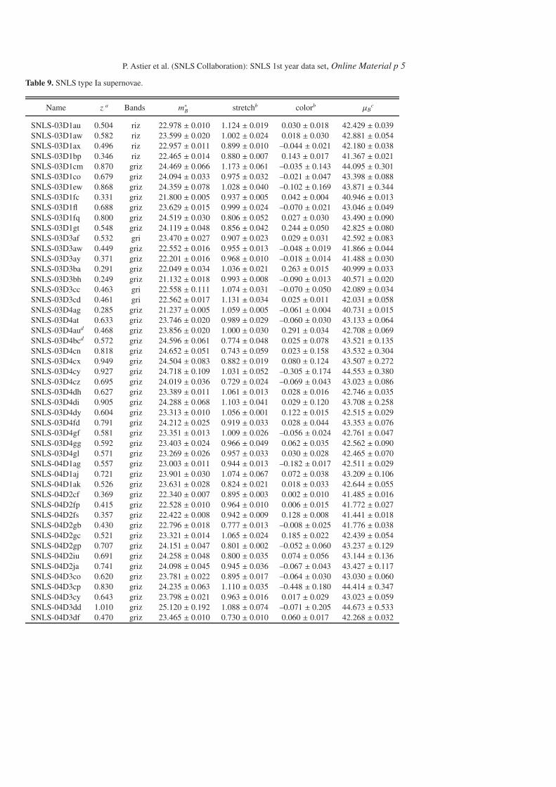
P. Astier et al. (SNLS Collaboration): SNLS 1st year data set, Online Material p 5

Table 9. SNLS type Ia supernovae.

Name z a Bands m∗B stretchb colorb µBc

SNLS-03D1au 0.504 riz 22.978 ± 0.010 1.124 ± 0.019 0.030 ± 0.018 42.429 ± 0.039SNLS-03D1aw 0.582 riz 23.599 ± 0.020 1.002 ± 0.024 0.018 ± 0.030 42.881 ± 0.054SNLS-03D1ax 0.496 riz 22.957 ± 0.011 0.899 ± 0.010 –0.044 ± 0.021 42.180 ± 0.038SNLS-03D1bp 0.346 riz 22.465 ± 0.014 0.880 ± 0.007 0.143 ± 0.017 41.367 ± 0.021SNLS-03D1cm 0.870 griz 24.469 ± 0.066 1.173 ± 0.061 –0.035 ± 0.143 44.095 ± 0.301SNLS-03D1co 0.679 griz 24.094 ± 0.033 0.975 ± 0.032 –0.021 ± 0.047 43.398 ± 0.088SNLS-03D1ew 0.868 griz 24.359 ± 0.078 1.028 ± 0.040 –0.102 ± 0.169 43.871 ± 0.344SNLS-03D1fc 0.331 griz 21.800 ± 0.005 0.937 ± 0.005 0.042 ± 0.004 40.946 ± 0.013SNLS-03D1fl 0.688 griz 23.629 ± 0.015 0.999 ± 0.024 –0.070 ± 0.021 43.046 ± 0.049SNLS-03D1fq 0.800 griz 24.519 ± 0.030 0.806 ± 0.052 0.027 ± 0.030 43.490 ± 0.090SNLS-03D1gt 0.548 griz 24.119 ± 0.048 0.856 ± 0.042 0.244 ± 0.050 42.825 ± 0.080SNLS-03D3af 0.532 gri 23.470 ± 0.027 0.907 ± 0.023 0.029 ± 0.031 42.592 ± 0.083SNLS-03D3aw 0.449 griz 22.552 ± 0.016 0.955 ± 0.013 –0.048 ± 0.019 41.866 ± 0.044SNLS-03D3ay 0.371 griz 22.201 ± 0.016 0.968 ± 0.010 –0.018 ± 0.014 41.488 ± 0.030SNLS-03D3ba 0.291 griz 22.049 ± 0.034 1.036 ± 0.021 0.263 ± 0.015 40.999 ± 0.033SNLS-03D3bh 0.249 griz 21.132 ± 0.018 0.993 ± 0.008 –0.090 ± 0.013 40.571 ± 0.020SNLS-03D3cc 0.463 gri 22.558 ± 0.111 1.074 ± 0.031 –0.070 ± 0.050 42.089 ± 0.034SNLS-03D3cd 0.461 gri 22.562 ± 0.017 1.131 ± 0.034 0.025 ± 0.011 42.031 ± 0.058SNLS-03D4ag 0.285 griz 21.237 ± 0.005 1.059 ± 0.005 –0.061 ± 0.004 40.731 ± 0.015SNLS-03D4at 0.633 griz 23.746 ± 0.020 0.989 ± 0.029 –0.060 ± 0.030 43.133 ± 0.064SNLS-03D4aud 0.468 griz 23.856 ± 0.020 1.000 ± 0.030 0.291 ± 0.034 42.708 ± 0.069SNLS-03D4bcd 0.572 griz 24.596 ± 0.061 0.774 ± 0.048 0.025 ± 0.078 43.521 ± 0.135SNLS-03D4cn 0.818 griz 24.652 ± 0.051 0.743 ± 0.059 0.023 ± 0.158 43.532 ± 0.304SNLS-03D4cx 0.949 griz 24.504 ± 0.083 0.882 ± 0.019 0.080 ± 0.124 43.507 ± 0.272SNLS-03D4cy 0.927 griz 24.718 ± 0.109 1.031 ± 0.052 –0.305 ± 0.174 44.553 ± 0.380SNLS-03D4cz 0.695 griz 24.019 ± 0.036 0.729 ± 0.024 –0.069 ± 0.043 43.023 ± 0.086SNLS-03D4dh 0.627 griz 23.389 ± 0.011 1.061 ± 0.013 0.028 ± 0.016 42.746 ± 0.035SNLS-03D4di 0.905 griz 24.288 ± 0.068 1.103 ± 0.041 0.029 ± 0.120 43.708 ± 0.258SNLS-03D4dy 0.604 griz 23.313 ± 0.010 1.056 ± 0.001 0.122 ± 0.015 42.515 ± 0.029SNLS-03D4fd 0.791 griz 24.212 ± 0.025 0.919 ± 0.033 0.028 ± 0.044 43.353 ± 0.076SNLS-03D4gf 0.581 griz 23.351 ± 0.013 1.009 ± 0.026 –0.056 ± 0.024 42.761 ± 0.047SNLS-03D4gg 0.592 griz 23.403 ± 0.024 0.966 ± 0.049 0.062 ± 0.035 42.562 ± 0.090SNLS-03D4gl 0.571 griz 23.269 ± 0.026 0.957 ± 0.033 0.030 ± 0.028 42.465 ± 0.070SNLS-04D1ag 0.557 griz 23.003 ± 0.011 0.944 ± 0.013 –0.182 ± 0.017 42.511 ± 0.029SNLS-04D1aj 0.721 griz 23.901 ± 0.030 1.074 ± 0.067 0.072 ± 0.038 43.209 ± 0.106SNLS-04D1ak 0.526 griz 23.631 ± 0.028 0.824 ± 0.021 0.018 ± 0.033 42.644 ± 0.055SNLS-04D2cf 0.369 griz 22.340 ± 0.007 0.895 ± 0.003 0.002 ± 0.010 41.485 ± 0.016SNLS-04D2fp 0.415 griz 22.528 ± 0.010 0.964 ± 0.010 0.006 ± 0.015 41.772 ± 0.027SNLS-04D2fs 0.357 griz 22.422 ± 0.008 0.942 ± 0.009 0.128 ± 0.008 41.441 ± 0.018SNLS-04D2gb 0.430 griz 22.796 ± 0.018 0.777 ± 0.013 –0.008 ± 0.025 41.776 ± 0.038SNLS-04D2gc 0.521 griz 23.321 ± 0.014 1.065 ± 0.024 0.185 ± 0.022 42.439 ± 0.054SNLS-04D2gp 0.707 griz 24.151 ± 0.047 0.801 ± 0.002 –0.052 ± 0.060 43.237 ± 0.129SNLS-04D2iu 0.691 griz 24.258 ± 0.048 0.800 ± 0.035 0.074 ± 0.056 43.144 ± 0.136SNLS-04D2ja 0.741 griz 24.098 ± 0.045 0.945 ± 0.036 –0.067 ± 0.043 43.427 ± 0.117SNLS-04D3co 0.620 griz 23.781 ± 0.022 0.895 ± 0.017 –0.064 ± 0.030 43.030 ± 0.060SNLS-04D3cp 0.830 griz 24.235 ± 0.063 1.110 ± 0.035 –0.448 ± 0.180 44.414 ± 0.347SNLS-04D3cy 0.643 griz 23.798 ± 0.021 0.963 ± 0.016 0.017 ± 0.029 43.023 ± 0.059SNLS-04D3dd 1.010 griz 25.120 ± 0.192 1.088 ± 0.074 –0.071 ± 0.205 44.673 ± 0.533SNLS-04D3df 0.470 griz 23.465 ± 0.010 0.730 ± 0.010 0.060 ± 0.017 42.268 ± 0.032

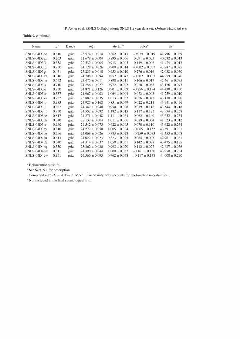
P. Astier et al. (SNLS Collaboration): SNLS 1st year data set, Online Material p 6

Table 9. continued.

Name z a Bands m∗B stretchb colorb µBc

SNLS-04D3do 0.610 griz 23.574 ± 0.014 0.862 ± 0.013 –0.079 ± 0.019 42.796 ± 0.039SNLS-04D3ez 0.263 griz 21.678 ± 0.004 0.895 ± 0.006 0.091 ± 0.003 40.682 ± 0.013SNLS-04D3fk 0.358 griz 22.532 ± 0.005 0.913 ± 0.005 0.149 ± 0.006 41.474 ± 0.013SNLS-04D3fq 0.730 griz 24.128 ± 0.026 0.900 ± 0.014 –0.002 ± 0.037 43.287 ± 0.075SNLS-04D3gt 0.451 griz 23.235 ± 0.010 0.953 ± 0.010 0.276 ± 0.016 42.038 ± 0.030SNLS-04D3gx 0.910 griz 24.708 ± 0.094 0.952 ± 0.047 –0.202 ± 0.163 44.259 ± 0.346SNLS-04D3hn 0.552 griz 23.475 ± 0.011 0.898 ± 0.011 0.106 ± 0.017 42.461 ± 0.035SNLS-04D3is 0.710 griz 24.256 ± 0.027 0.972 ± 0.002 0.220 ± 0.038 43.176 ± 0.077SNLS-04D3ki 0.930 griz 24.871 ± 0.126 0.901 ± 0.039 –0.256 ± 0.194 44.430 ± 0.430SNLS-04D3kr 0.337 griz 21.967 ± 0.003 1.064 ± 0.004 0.072 ± 0.003 41.259 ± 0.010SNLS-04D3ks 0.752 griz 23.882 ± 0.035 1.013 ± 0.037 0.026 ± 0.043 43.170 ± 0.090SNLS-04D3lp 0.983 griz 24.925 ± 0.168 0.831 ± 0.049 0.022 ± 0.211 43.941 ± 0.496SNLS-04D3lu 0.822 griz 24.342 ± 0.040 0.950 ± 0.028 0.019 ± 0.116 43.544 ± 0.218SNLS-04D3ml 0.950 griz 24.552 ± 0.082 1.182 ± 0.015 0.117 ± 0.122 43.954 ± 0.268SNLS-04D3nc 0.817 griz 24.271 ± 0.048 1.111 ± 0.064 0.062 ± 0.140 43.652 ± 0.254SNLS-04D3nh 0.340 griz 22.137 ± 0.004 1.011 ± 0.006 0.089 ± 0.004 41.323 ± 0.012SNLS-04D3nr 0.960 griz 24.542 ± 0.075 0.922 ± 0.045 0.070 ± 0.110 43.622 ± 0.234SNLS-04D3ny 0.810 griz 24.272 ± 0.050 1.005 ± 0.084 –0.065 ± 0.152 43.691 ± 0.301SNLS-04D3oe 0.756 griz 24.069 ± 0.026 0.783 ± 0.028 –0.259 ± 0.033 43.453 ± 0.058SNLS-04D4an 0.613 griz 24.022 ± 0.023 0.823 ± 0.025 0.064 ± 0.025 42.961 ± 0.061SNLS-04D4bk 0.840 griz 24.314 ± 0.037 1.050 ± 0.051 0.142 ± 0.098 43.475 ± 0.185SNLS-04D4bq 0.550 griz 23.362 ± 0.020 0.995 ± 0.029 0.112 ± 0.027 42.487 ± 0.056SNLS-04D4dm 0.811 griz 24.390 ± 0.044 1.000 ± 0.057 –0.161 ± 0.150 43.950 ± 0.264SNLS-04D4dw 0.961 griz 24.566 ± 0.093 0.962 ± 0.058 –0.117 ± 0.138 44.000 ± 0.290

a Heliocentric redshift.b See Sect. 5.1 for description.c Computed with H0 = 70 km s−1 Mpc−1. Uncertainty only accounts for photometric uncertainties.d Not included in the final cosmological fits.