Embed Size (px)
Citation preview
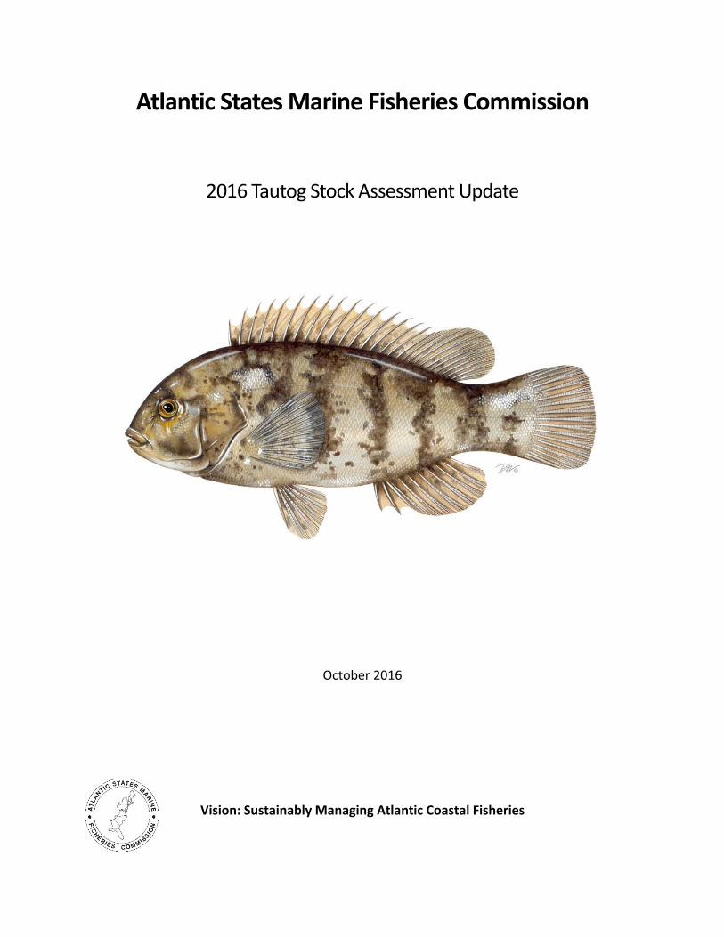
Atlantic States Marine Fisheries Commission
2016 Tautog Stock Assessment Update
October 2016
Vision: Sustainably Managing Atlantic Coastal Fisheries

Tautog Stock Assessment Update ii
Prepared by the Tautog Technical Committee and Stock Assessment Subcommittee
Jason McNamee, TC Chair, Rhode Island Division of Fish and Wildlife Jeffrey Brust, SASC Chair, New Jersey Division of Fish and Wildlife Nichole Ares, Rhode Island Division of Fish and Wildlife Deborah Pacileo, Connecticut Department of Energy and Environmental Protection Sandra Dumais, New York State Department of Environmental Conservation Linda Barry, New Jersey Division of Fish and Wildlife Scott Newlin, Delaware Division of Fish and Wildlife Alexei Sharov, Maryland Department of Natural Resources Craig Weedon, Maryland Department of Natural Resources Katie May Laumann, Virginia Marine Resources Commission Tom Wadsworth, North Carolina Division of Marine Fisheries Katie Drew, Atlantic States Marine Fisheries Commission Ashton Harp, Atlantic States Marine Fisheries Commission
In collaboration with the Tautog Long Island Sound Regional Working Group
Jacob Kasper, University of Connecticut Eric Schultz, University of Connecticut Greg Wojcik, Connecticut Department of Energy and Environmental Protection

Tautog Stock Assessment Update iii
Table of Contents
List of Tables and Figures ......................................................................................................... iv Executive Summary ............................................................................................................... viii 1 Stock Identification ............................................................................................................... 1 2 Life History ........................................................................................................................... 1 3 Data ...................................................................................................................................... 1 3.1 Massachusetts‐Rhode Island ................................................................................................ 2 3.2 Long Island Sound ................................................................................................................. 3 3.3 New Jersey – New York Bight ............................................................................................... 3 3.4 DelMarVa .............................................................................................................................. 5 3.5 Coastwide .............................................................................................................................. 7
4 Model ................................................................................................................................... 8 4.1 Massachusetts‐Rhode Island ................................................................................................ 8 4.2 Long Island Sound ................................................................................................................. 8 4.3 New Jersey‐New York Bight .................................................................................................. 9 4.4 DelMarVa .............................................................................................................................. 9 4.5 Coastwide ............................................................................................................................ 10
5 Results ................................................................................................................................ 10 5.1 Massachusetts – Rhode Island ............................................................................................ 10 5.2 Long Island Sound ............................................................................................................... 11 5.3 New Jersey – New York Bight ............................................................................................. 12 5.4 DelMarVa ............................................................................................................................ 14 5.5 Coastwide ............................................................................................................................ 15
6 Biological Reference Points and Stock Status ...................................................................... 16 6.1 Massachusetts‐Rhode Island .............................................................................................. 17 6.2 Long Island Sound ............................................................................................................... 17 6.3 New Jersey – New York Bight ............................................................................................. 18 6.4 DelMarVa ............................................................................................................................ 18 6.5 Coastwide ............................................................................................................................ 19
7 Projections ......................................................................................................................... 19 7.1 Massachusetts – Rhode Island ............................................................................................ 19 7.2. Long Island Sound .............................................................................................................. 20 7.3 New Jersey – New York Bight ............................................................................................. 20 7.4 DelMarVa ............................................................................................................................ 21 7.5 Coastwide ............................................................................................................................ 21
8 Research Recommendations ............................................................................................... 22 9 Literature Cited................................................................................................................... 22 10 Tables ............................................................................................................................... 23 11 Figures .............................................................................................................................. 49
Tautog Stock Assessment Update iv
List of Tables and Figures Table 3.1.1. Total removals by sector for the MARI region. ......................................................... 23 Table 3.1.2. Indices of relative abundance for the MARI region. ................................................. 24 Table 3.2.1. Total catch by sector for the LIS region. ................................................................... 25 Table 3.2.2. Indices of abundance for the LIS region. .................................................................. 26 Table 3.3.1. Total catch by sector for the NJ‐NYB region. ............................................................ 27 Table 3.3.2 Indices of relative of abundance for the NJ‐NYB region ............................................ 28 Table 3.4.1. Total catch by sector for the DMV region. ................................................................ 29 Table 3.4.2. Indices of relative abundance for the DMV region. .................................................. 30 Table 3.5.1. Total catch by sector for the coast. .......................................................................... 31 Table 3.5.2. Indices of relative abundance for the coast (Age‐1+). .............................................. 32 Table 3.5.3. Recruitment indices for the coast. ............................................................................ 33 Table 5.1.1. Fishing mortality estimates for the MARI region ...................................................... 34 Table 5.1.2 Spawning stock biomass and recruitment estimates for the MARI region ............... 35 Table 5.2.1. Fishing mortality estimates for the LIS region. ......................................................... 36 Table 5.2.2. Spawning stock biomass and recruitment estimates for the LIS region. ................. 37 Table 5.3.1. Fishing mortality estimates for the NJ‐NYB region. .................................................. 38 Table 5.3.2. Spawning stock biomass and recruitment estimates for the NJ‐NYB region. .......... 39 Table 5.4.1. Fishing mortality estimates for the DMV region. ..................................................... 40 Table 5.4.2. Spawning stock biomass and recruitment estimates for the DMV region. .............. 41 Table 5.5.1. Fishing mortality estimates for the coast. ................................................................ 42 Table 5.5.2. Spawning stock biomass and recruitment estimates for the coast. ......................... 43 Table 7.1.1. Short‐term projection results for the MARI region. ................................................. 44 Table 7.2.1. Short‐term projection results for the LIS region. ...................................................... 45 Table 7.3.1. Short‐term projection results for the NJ‐NYB region. .............................................. 46 Table 7.4.1. Short‐term projection results for the DMV region. .................................................. 47 Table 7.5.1. Short‐term projection results for the coast. ............................................................. 48 Figure 3.1.3. RI Fall Trawl Survey index of abundance. ................................................................ 51 Figure 3.1.4. RI Seine Survey young‐of‐year index of abundance. ............................................... 52 Figure 3.1.5. MRIP CPUE for the MARI region. ............................................................................. 53 Figure 3.2.2. CT Long Island Sound Trawl Survey index of abundance. ....................................... 55 Figure 3.2.3. MRIP CPUE for the LIS region. ................................................................................. 56 Figure 3.2.4. NY Peconic Bay Trawl Survey YOY index. ................................................................. 57 Figure 3.2.5. NY Western Long Island Seine Survey YOY index for the LIS region. ...................... 58 Figure 3.3.1. Total removals by sector for the NJ‐NYB region. ..................................................... 59 Figure 3.3.2. NY Western Long Island Seine Survey YOY index for the NJ‐NYB region. ............... 60 Figure 3.3.3. NJ Ocean Trawl index of abundance. ...................................................................... 61 Figure 3.3.4. MRIP CPUE for the NJ‐NYB region. .......................................................................... 62 Figure 3.4.2. MRIP CPUE for the DMV region. .............................................................................. 64 Figure 3.5.1. Total removals by sector for the coast. ................................................................... 65 Figure 3.5.2. Coastwide removals by region ................................................................................. 66 Figure 3.5.3. Comparison of regional and coastwide MRIP CPUE trends. ................................... 67 Figure 3.5.4. Comparison of fishery independent age‐1+ index trends for the coast. ................ 68
Tautog Stock Assessment Update v
Figure 3.5.5. Comparison of fishery independent recruitment index trends for the coast. ........ 69 Figure 5.1.1. Estimated selectivity patterns for the fishery in the MARI region. ......................... 70 Figure 5.1.2. Fishing mortality estimates for the MARI region. ................................................... 71 Figure 5.1.3. Spawning stock biomass estimates for the MARI region. ....................................... 72 Figure 5.1.4. Abundance at age for the MARI region. .................................................................. 73 Figure 5.1.5. Recruitment estimates for the MARI region. .......................................................... 74 Figure 5.1.6. Stock‐recruitment relationship for the MARI region. .............................................. 75 Figure 5.1.7. Retrospective analysis for the MARI region ............................................................ 76 Figure 5.2.1 Estimated selectivity patterns for the fishery in the LIS region. .............................. 77 Figure 5.2.2 Annual fishing mortality (F) and 3‐year average for LIS. .......................................... 78 Figure 5.2.3. Estimates of spawning stock biomass for the LIS region. ........................................ 79 Figure 5.2.4. Abundance at age for the LIS region. ...................................................................... 80 Figure 5.2.5. Recruitment estimates for LIS region ...................................................................... 81 Figure 5.2.6. Stock‐recruitment relationship for the MARI region. .............................................. 82 Figure 5.2.7. Retrospective analysis for LIS region ....................................................................... 83 Figure 5.3.1. Estimated selectivity patterns for the NJ‐NYB region. ............................................ 84 Figure 5.3.2. Fishing mortality estimates for the NJ‐NYB region. ................................................. 85 Figure 5.3.3. Spawning stock biomass estimates for the NJ‐NYB region. .................................... 86 Figure 5.3.4. Abundance at age for the NJ‐NYB region ................................................................ 87 Figure 5.3.5. Recruitment estimates for the NJ‐NYB region. ....................................................... 88 Figure 5.3.6. Stock‐recruitment data for NJ‐NYB region. ............................................................. 89 Figure 5.3.7. Retrospective analysis for the NJ‐NYB region ......................................................... 90 Figure 5.4.1. Estimated selectivity patterns for the DMV region. ................................................ 91 Figure 5.4.2. Fishing mortality estimates for the DMV region. .................................................... 92 Figure 5.4.3. Spawning stock biomass estimates for the DMV region. ........................................ 93 Figure 5.4.4. Abundance at age for the DMV region .................................................................... 94 Figure 5.4.5. Recruitment estimates for the DMV region. ........................................................... 95 Figure 5.4.6. Stock‐recruitment data for the DMV region. .......................................................... 96 Figure 5.4.7. Retrospective analysis for the DMV region. ............................................................ 97 Figure 5.5.1. Estimated selectivity patterns for the coast. ........................................................... 98 Figure 5.5.2. Fishing mortality estimates for the coast. ............................................................... 99 Figure 5.5.3. Spawning stock biomass estimates for the coast. ................................................. 100 Figure 5.5.4. Abundance at age for the coast ............................................................................. 101 Figure 5.5.5. Recruitment estimates for the coast. .................................................................... 102 Figure 5.5.6. Stock‐recruitment curve for the coast. .................................................................. 103 Figure 5.5.7. Retrospective analysis for the coast. ..................................................................... 104 Figure 6.1.1. F (top) and SSB (bottom) plotted with their MSY‐based targets and thresholds for the MARI region. ......................................................................................................................... 105 Figure 6.1.2. F (top) and SSB (bottom) plotted with their SPR‐based targets and thresholds for the MARI region ................................................................................................................................ 106 Figure 6.2.1. F (top) and SSB (bottom) plotted with their MSY‐based targets and thresholds for the LIS region. ............................................................................................................................. 107 Figure 6.2.2. F (top) and SSB (bottom) plotted with their SPR‐based targets and thresholds for the LIS region. .................................................................................................................................... 108
Tautog Stock Assessment Update vi
Figure 6.3.1. F (top) and SSB (bottom) plotted with their SPR‐based targets and thresholds for the NJ‐NYB region ............................................................................................................................. 109 Figure 6.4.1. F (top) and SSB (bottom) plotted with their SPR‐based targets and thresholds for the DMV region. ................................................................................................................................ 110 Figure 6.5.3. F (top) and SSB (bottom) plotted with their SPR‐based targets and thresholds for the coast. ........................................................................................................................................... 112 Figure 7.1.1. Short‐term projection results for F (top) and SSB (bottom) under status quo landings for the MARI region relative to MSY reference points. .............................................................. 113 Figure 7.1.2. Short‐term projection results for F (top) and SSB (bottom) under status quo landings for the MARI region relative to SPR reference points. ............................................................... 114 Figure 7.1.3. Short‐term projection results for F (top) and SSB (bottom) with a 50% probability of achieving F target in 2020 for the MARI region using MSY reference points. ........................... 115 Figure 7.1.4. Short‐term projection results for F (top) and SSB (bottom) with a 70% probability of achieving F target in 2020 for the MARI region using MSY reference points. ........................... 116 Figure 7.1.5. Short‐term projection results for F (top) and SSB (bottom) with a 50% probability of achieving F target in 2020 for the MARI region using SPR reference points. ............................ 117 Figure 7.1.6. Short‐term projection results for F (top) and SSB (bottom) with a 70% probability of achieving F target in 2020 for the MARI region using SPR reference points. ............................ 118 Figure 7.2.1 Short‐term projection results for F (top) and SSB (bottom) under status quo landings for the LIS region relative to MSY reference points. .................................................................. 119 Figure 7.2.2 Short‐term projection results for F (top) and SSB (bottom) with a 50% probability of achieving F target in 2020 for the LIS region using MSY reference points. ................................ 120 Figure 7.2.3. Short‐term projection results for F (top) and SSB (bottom) with a 70% probability of achieving F target in 2020 for the LIS region using MSY reference points. ................................ 121 Figure 7.2.4. Short‐term projection results for F (top) and SSB (bottom) with a 50% probability of achieving F target in 2020 for the LIS region using SPR reference points. ................................. 122 Figure 7.2.5. Short‐term projection results for F (top) and SSB (bottom) with a 70% probability of achieving F target in 2020 for the LIS region using SPR reference points. ................................. 123 Figure 7.3.1. Short‐term projection results for F (top) and SSB (bottom) with a 50% probability of achieving F target in 2020 for the NJ‐NYB region. ...................................................................... 124 Figure 7.3.2. Short‐term projection results for F (top) and SSB (bottom) with a 70% probability of achieving F target in 2020 for the NJ‐NYB region. ...................................................................... 125 Figure 7.4.1. Short‐term projections of F (top) and SSB (bottom) under status quo harvest scenario for the DMV region. ..................................................................................................... 126 Figure 7.4.2. Short‐term projection results for F (top) and SSB (bottom) with a 50% probability of achieving F target in 2020 for the DMV region. ......................................................................... 127 Figure 7.4.3. Short‐term projection results for F (top) and SSB (bottom) with a 70% probability of achieving F target in 2020 for the DMV region. ......................................................................... 128 Figure 7.5.1. Short‐term projection results for F (top) and SSB (bottom) under the status quo harvest scenario for the coast relative to MSY‐based reference points. ................................... 129 Figure 7.5.2. Short‐term projection results for F (top) and SSB (bottom) with a 50% probability of achieving F target in 2020 for the coast using MSY‐based reference points. ............................ 130 Figure 7.5.3. Short‐term projection results for F (top) and SSB (bottom) with a 70% probability of achieving F target in 2020 for the coast using MSY‐based reference points. ............................ 131
Tautog Stock Assessment Update vii
Figure 7.5.4. Short‐term projections for F (top) and SSB (bottom) under the status quo harvest scenario for the coast relative to SPR‐based reference points. ................................................. 132 Figure 7.5.5. Short‐term projection results for F (top) and SSB (bottom) with a 50% probability of achieving F target in 2020 for the coast using SPR‐based reference points. ............................. 133 Figure 7.5.6. Short‐term projection results for F (top) and SSB (bottom) with a 70% probability of achieving F target in 2020 for the coast using SPR‐based reference points. ............................. 134
Tautog Stock Assessment Update viii
Executive Summary The regions accepted for management use are defined as:
‐ Massachusetts ‐ Rhode Island (MARI) ‐ Long Island Sound (LIS), which consists of Connecticut and New York waters north of Long
Island ‐ New Jersey – New York Bight (NJ‐NYB), which consists of New Jersey and New York waters
south of Long Island ‐ Delaware, Maryland and Virginia (DelMarVa)
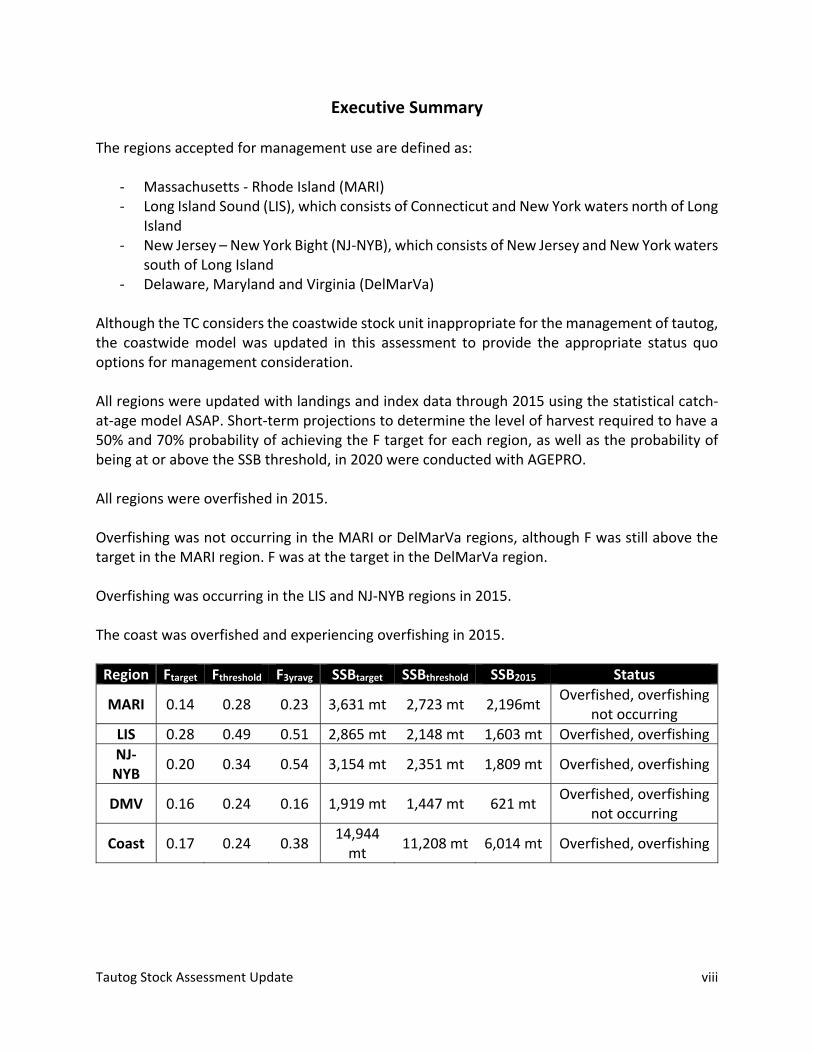
Although the TC considers the coastwide stock unit inappropriate for the management of tautog, the coastwide model was updated in this assessment to provide the appropriate status quo options for management consideration. All regions were updated with landings and index data through 2015 using the statistical catch‐at‐age model ASAP. Short‐term projections to determine the level of harvest required to have a 50% and 70% probability of achieving the F target for each region, as well as the probability of being at or above the SSB threshold, in 2020 were conducted with AGEPRO. All regions were overfished in 2015. Overfishing was not occurring in the MARI or DelMarVa regions, although F was still above the target in the MARI region. F was at the target in the DelMarVa region. Overfishing was occurring in the LIS and NJ‐NYB regions in 2015. The coast was overfished and experiencing overfishing in 2015.
Region Ftarget Fthreshold F3yravg SSBtarget SSBthreshold SSB2015 Status
MARI 0.14 0.28 0.23 3,631 mt 2,723 mt 2,196mt Overfished, overfishing
not occurring
LIS 0.28 0.49 0.51 2,865 mt 2,148 mt 1,603 mt Overfished, overfishing
NJ‐NYB
0.20 0.34 0.54 3,154 mt 2,351 mt 1,809 mt Overfished, overfishing
DMV 0.16 0.24 0.16 1,919 mt 1,447 mt 621 mt Overfished, overfishing
not occurring
Coast 0.17 0.24 0.38 14,944 mt
11,208 mt 6,014 mt Overfished, overfishing

Tautog Stock Assessment Update ix
The MARI, LIS, and coast need to take harvest reductions in order to have a 50% or 70% probability of being at the Ftarget in 2020. These range from a 55‐56% reduction from 2015 levels in MARI and a 47‐53% reduction from 2015 levels in LIS, to an 18‐24% reduction from 2015 levels for the coast. Harvest levels for the NJ‐NYB and DMV region that are at or slightly above 2015 levels will result in a 50‐70% probability of F being at or below Ftarget for those regions. Even at the target F levels, the probability of SSB being above the SSBthreshold in 2020 is small for all regions.
Tautog Stock Assessment Update 1
1 Stock Identification Historically, tautog has been assessed as a coastwide stock, consistent with the management unit, which includes all states from Massachusetts through Virginia. In the 2015 benchmark stock assessment (ASMFC 2015), the Tautog TC investigated new stock unit definitions based on life history data, fishery and habitat characteristics, and available data sources. A subsequent 2016 regional assessment analyzes two additional regions to comprise a four‐region management scenario (ASMFC 2016). The regions used in this assessment update are defined as:
‐ Massachusetts ‐ Rhode Island (MARI) ‐ Long Island Sound (LIS), which consists of Connecticut and New York waters north of
Long Island ‐ New Jersey – New York Bight (NJ‐NYB), which consists of New Jersey and New York
waters south of Long Island ‐ Delaware, Maryland and Virginia (DelMarVa)
Although the TC considers the coastwide stock unit inappropriate for the management of tautog, the coastwide model was updated in this assessment to provide the appropriate status quo options for management consideration.
2 Life History Tautog are a relatively slow growing, long‐lived fish. Individuals over 30 years have been recorded in Rhode Island, Connecticut, and Virginia. Tautog also grow to large sizes, up to 11.36 kg (25 lbs). They mature at 3 to 4 years of age, and spawn from April – September. They undergo seasonal inshore‐offshore migration in some parts of their range, but tagging data indicate they return to the same reefs year after year and do not make extensive north‐south migrations. The 2015 benchmark assessment explored a number of different ways of estimating natural mortality (M). Maximum age based methods gave a result of M=0.15 for most regions and M=0.16 for the DelMarVa region, consistent with what has been used in previous assessments.
3 Data The MARI, DelMarVa, and coastwide update assessments use the same data sources as the 2015 benchmark stock assessment. The LIS and NJ‐NYB update assessments use the same data sources as the 2016 regional assessment. All regions incorporate data through 2015. The recreational discard mortality rate of 2.5% was used for all regions.
Tautog Stock Assessment Update 2
3.1 Massachusetts‐Rhode Island
3.1.1 Landings Recreational anglers account for upwards of 90% of landings in this region. In the MARI region, recreational landings peaked in 1986 at nearly 2.7 million fish and fell sharply to about 13% of its peak by the mid‐1990s. Since then landings have remained low and have varied in the range of 200,000 to 50,000 fish. The 2013‐2015 average recreational landings are 167,085 fish (Table 3.1.1, Figure 3.1.1). The majority (nearly 75%) of tautog recreational harvest in the MARI region comes from the private/rental boat mode. The remaining 25% is split relatively evenly among the shore and for‐hire (party/charter boat) modes. Commercial landings in the MARI region peaked in 1991 at approximately 725,300 lbs (329 mt), declined to 97,000 lbs (44 mt) in 1996, and since then has varied in the range of 110,000 – 200,000 lbs (50 to 90 mt) (Table 3.1.1, Figure 3.1.1). The 2013‐2015 average landings in the MARI region were approximately 121,250 lbs (55 mt). Total removals in the MARI region, including recreation harvest, recreational release mortality, and commercial landings averaged 390 mt, with 337 mt taken in 2015.
3.1.2 Indices The set of indices available in the MARI region consists of two trawl survey indices, one seine survey which aliases the young of the year segment of the population, and a fishery dependent index using MRIP information (Table 3.1.2, Figures 3.3.2‐5). For all indices, statistical model‐based standardization of the survey data was conducted to account for factors that affect tautog catchability. The Massachusetts Division of Marine Fisheries (MADMF) runs a synoptic coastal trawl survey performed in the spring and autumn utilizing a stratified random design. The Rhode Island Division of Fish and Wildlife (RIDFW) research trawl survey has two components, a seasonal survey with a random stratified design which began in 1979, and a monthly fixed station survey which began in 1990 that is conducted monthly throughout the year. For the tautog stock assessment only the fall segment of the RI trawl survey was used, consistent with the benchmark assessment. The RI Seine Survey has operated from 1986 to the present, with a consistent standardized consistent methodology starting in 1988. It is a fixed site survey that takes place throughout the extent of Narragansett Bay Rhode Island. The Tautog TC developed a fishery dependent index of abundance from MRIP recreational survey data, using “logical guilds” to identify tautog trips.
Tautog Stock Assessment Update 3
3.1.3 Biosampling and Age‐Length Keys For the MARI region, age‐length samples are collected from a combination of recreational fishermen and fishery independent surveys. There was a total of 756 length‐age samples collected in the MARI region from 2013‐2015 (approximately 250 per year) to characterize the age structure in the region.
3.2 Long Island Sound 3.2.1 Landings
The update assessment estimates of commercial and recreational landings and recreational discards (Table 3.2.1, Figure 3.2.1) have been revised in all years from those used in the previous LIS regional assessment (ASMFC 2015). Total removals in LIS (recreational harvest, recreational dead discards and commercial harvest) peaked in 1987 at 1,386 mt. In recent years landings have been a fraction of that; for example, the 2015 landings were 430 mt or 21% of the peak. Commercial harvest accounts for approximately 12% of total catch, recreational harvest accounts for 86% and recreational discards for about 2%.
3.1.1 Indices The model was fit to both the total standardized index (catch per tow or catch per trip) and index‐at‐age of the Connecticut Long Island Sound Trawl Survey and MRIP CPUE (Table 3.2.2, Figure 3.2.2‐3). The New York Peconic Bay Trawl Survey (Table 3.2.2. Figure 3.2.4) was used as a year one index. The New York Western Long Island Seine Survey (Table 3.2.2, Figure 3.2.5) was treated as a young‐of‐year index and was lagged forward one year (e.g., the observed 1984 YOY index value was represented as the predicted 1985 age‐1 index value).
3.1.2 Biosampling and Age‐Length Keys The update assessment uses an ALK that has been updated from the previous LIS regional assessment (ASMFC 2015) upon incorporation of 2015 fishery independent indices. Data used in the LIS ALKs include LISTS, the Rhode Island Trawl Survey (RI) and New York Port Sampling (NY‐N) (Table 3.2.3). An average of 415 samples were used per year with a minimum sample size of 109 and a max of 859. Rhode Island age‐length data were included as needed to a fill size gaps in the key. New York data included only fish that were collected from the North Shore of Long Island. Size gaps that remained were filled using age distributions estimated from a key that pooled all years of data. The length range of the ALK is narrower than the estimated catch (ALK: 15 to 60 cm; estimated catch: 8 to 83 cm). Lengths below 16 cm and above 60 cm were accordingly binned into single groups.
3.3 New Jersey – New York Bight
3.3.1 Landings Tautog is predominantly a recreationally caught species, with anglers accounting for about 90% of landings within the NJ‐NYB region. Between 2013 and 2015, annual recreational landings have shown high interannual variability without a trend, ranging from approximately 150,000 to
Tautog Stock Assessment Update 4
400,000 fish, with an average of 242,000 fish (Table 3.3.1, Figure 3.3.1). For this assessment update, a change was made to how New York recreational harvest was split between LIS and south shore for the years 2004+. The June 2016 regional assessment used a post‐stratification SAS code to separate harvest from the two regions, but this method does not weight sites based on activity. For this update, harvest by region was estimated using MRIP data which does account for site activity. Seven of eleven years are within 10% of the value used in the benchmark assessment, but four years (2007, 2009, 2010, and 2013) resulted in increases of 13% to 45% using the new methodology. In the NJ‐NYB region, commercial harvest during 2013 to 2015 has shown a declining trend falling from 99,207 lbs (45 mt) in 2013 to nearly 86,000 lbs (39 mt) in 2015 with an average harvest of 90,389 lbs (41 mt) for this time period (Table 3.3.2, Figure 3.3.1). Trends in harvest can be obscured by high interannual variability in catch and relatively high harvest measurement error. An unquantified illegal live fish market contributes to uncertainty in harvest estimates.
3.3.2 Indices The Western Long Island (WLI) Seine Survey, New Jersey (NJ) Ocean Trawl Survey, and recreational survey were used in the assessment update. The NJ‐NYB portion (Jamaica Bay) of the WLI seine survey encompasses 19 different stations. As not all stations were sampled continuously, only the eight stations sampled annually in at least 20 years were included in the model. An abundance index for tautog was created using a negative binomial generalized linear model (GLM) including station and water temperature. The WLI seine index captures mainly age‐0 fish, so was lagged forward one year and treated as an age‐1 index. (This is an improvement over the 2016 regional assessment that did not lag the index appropriately.) The index identifies three periods of recruitment separated by 3‐5 years of near zero recruitment with successively higher peaks. There was a time series high of 2.7 fish per tow in 2012, and an average catch of 1.5 fish for the period 2012‐2015 (Table 3.2.2, Figure 3.3.2). An abundance index for tautog was developed for the NJ Ocean Trawl survey using a negative binomial generalized linear model (GLM) including year, bottom temperature, depth, and bottom salinity as factors. The index was variable, but indicated a period of high abundance at the beginning of the time series, declined through the late 1990s, then recovered to moderate abundance between 2000 and 2010 (Table 3.3.2, Figure 3.3.3). CPUE dropped by more than 50% in 2011‐2012, but recovered to previous levels around 0.5 fish per tow in recent years. A fishery dependent index of abundance from the MRFSS/MRIP recreational survey data was developed using the logical guild methodology described in the regional benchmark assessment. Abundance was estimated using a negative binomial GLM, with the final model specified as
Tautog Stock Assessment Update 5
Total catch ~ Year + State + Wave + Mode, offset =ln(Angler_Hours). During development of this assessment update, it was determined that the recreational CPUE index used in the 2016 regional assessment for the NJ‐NYB region was incorrect. This error has been corrected for this assessment update. Generally, the two indices follow a similar pattern, but the corrected index exhibits slightly greater interannual variability. Results of the NJ‐NYB recreational CPUE index are shown in Table 3.3.2 and Figure 3.3.4. All three indices were used in the assessment model. The WLI seine index captures mainly age‐0 fish, so was lagged forward one year and treated as an age‐1 index. (This is an improvement over the 2016 regional assessment that did not lag the index appropriately.) The NJ ocean trawl and MRFSS indices were treated as adult indices (ages 1‐12+), with survey age distribution estimated using survey specific length frequency data and the NYNJ ALKs, assuming a plus group of ages 12+.
3.3.3 Biosampling and Age‐Length Keys For the NJ‐NYB region, recreational harvest length frequency was evaluated separately for NJ and NY south shore. Unweighted lengths from MRFSS/MRIP intercepts from NJ were the only source of information used to characterize recreational harvest length distributions in New Jersey, while the south shore harvest was characterized using combined region specific data from MRFSS/MRIP and the New York Headboat Survey (NYHBS) sampling program. The sum of the recreational harvest at length for NJ and NY south shore was used to estimate total regional harvest at length. As the tautog fishery is predominantly recreational, the length frequency distributions obtained from this sector were applied to the commercial harvest.
Numerous sources contributed to estimate the length frequency of discarded fish in the NJ‐NYB region. Region specific discard length data from the American Littoral Society Volunteer Angler Program (ALS) (1982‐present) and MRIP Type 9 sampling of fish released alive from headboats (2004‐present) were available for both NJ and south shore of NY. In addition, fishery dependent samples were also available for NY south from the NYHBS sampling program (1995‐present).
Prior to 1995, raw age data by state were not consistently available. As a result, ALKs for the NJ‐NYB region could only be created for 1995 forward. This still required pooling across regional boundaries to ensure the full range of sizes were covered by each regional key. As a result, the NJ‐NYB key includes some data from Long Island Sound and Delaware. The distribution of the NJ‐NYB harvest for the years 1989‐1994 was assumed to follow the same distribution as the age distribution of the NJ Ocean Trawl survey.
3.4 DelMarVa
3.4.1 Landings Recreational landings were obtained from the NMFS MRIP data collection program. Recreation harvest (A+B1) of tautog in DelMarVa has declined from 241,064 fish in 2010 to 22,215 in 2015
Tautog Stock Assessment Update 6
(Table 3.4.1, Figure 3.4.1). The decline coincided with the protective regulatory measures (minimum size increase and seasonal closures) instituted in 2012 to reduce fishing mortality. Recreational landings in 2015 were the lowest in time series. Recreational discards have also declined from 686,392 released fish in 2010 to 125,258 fish in 2015 (Table 3.4.1). Due to low number of intercepted fishing trips that had tautog, annual estimates of recreational landings and discards in MD and VA had low precision (Proportional Standard Error (PSE) values exceeded 50% in three out four of the most recent years). Commercial landings reported by each state (DE, MD, VA) in annual compliance reports were combined to derive region specific landings for the 2013‐2015 period and added to the time series compiled for the DelMarVa region in 2013 benchmark assessment. Commercial landings in DelMarVa region were declining in recent years, primarily due to a decline in Virginia (Table 3.4.1. and Figure 3.4.1). Average commercial landings for 2013‐2015 were 10,740 pounds (4.9 mt), with 2015 being much lower at 6,233 lbs (2.8 mt). Data on commercial discards were not available, but discards are believed to be minimal.
3.4.2 Indices There are no fishery independent indices available for the DelMarVa region. The only index of relative abundance used in the 2013 benchmark assessment was catch per trip derived from MRFSS / MRIP data. Total catch per trip was modeled with GLM method using a suite of potentially important covariates (year, state, wave, mode) with an effort offset based on angler hours for the trip. The MRIP based index was updated through 2015. The MRIP index suggested a continuing decline in the relative abundance of tautog in DelMarVa region (Table 3.4.2, Figure 3.4.2).
3.4.3 Biosampling and Age‐Length Keys Biological sampling for tautog is conducted by each state on annual basis with the goal to collect at least 200 samples per year for each state. Samples for length, weight, sex and age are taken mostly by intercepting the catch of recreational fishermen. However, some samples were taken from commercial fishery as well. Annual age length keys were constructed by combining paired length ‐ age samples from all three states. Total number of age and size samples used to construct annual ALK for 2013 ‐2015 ranged from 677 to 840, covering 23‐76 cm size range and ages 1‐29. Length frequency of the recreational harvest was characterized using length frequency of the data collected by MRIP for each state. State specific MRIP annual harvest estimates were applied to state specific length frequency of the recreational harvest (A+B1) to obtain harvest in numbers by size group. Size frequency of discards (B2) was characterized by combining the MRIP Type 9 and ALS raw data on the size of released fish by state. State specific data were pooled to obtain regional estimate of total harvest (A+B1) and discards. Due to low or absent commercial fishery size sampling, size frequency of recreational harvest was used to describe commercial catch at size. State specific recreational harvest, dead discards
Tautog Stock Assessment Update 7
and commercial harvest in numbers of fish by size were combined into regional estimate and converted into catch at age using regional year specific age length keys.
3.5 Coastwide 3.5.1 Landings
Coastwide recreational harvest peaked in 1986 at over 7 million fish and has declined since then (Table 3.5.1, Figure 3.5.1). Average recreational harvest from 2013‐2015 was 708,136 fish, with 2014 nearly double the harvest of 2013 and 2015: over 1 million fish compared to approximately 545,282 fish in 2015. The 2014 estimate was also more uncertain than the 2013 and 2015 estimates, with a PSE of 24.7% compared to 16‐17% in 2013 and 2015. The proportion of tautog released alive on the coast has increased over time. From 1982‐1986, an average of 17.7% of the catch was released alive, while from 2013‐2015, 81% of the catch was released alive (Figure 3.5.2). Tautog are very hardy; it is estimated that 2.5% of the fish that are released alive die as a result of being caught. This translates into an average of 73,551 tautog from 2013‐2015. Although the proportion of fish released alive was not significantly different in 2014, the total numbers of fish released alive was also nearly double the levels of 2013 and 2015. Commercial harvest showed a similar pattern to recreational harvest, although the magnitude is smaller, representing approximately 9% of the total harvest over the entire time series (Figure 3.5.3). It peaked in the late 1980s at 1.2 million lbs (525 mt), and declined to an average of 0.27 million lbs (124 mt) in 2013‐2015. Commercial harvest in 2014 was 0.28 million lbs (129 mt), not significantly different from the 2015 harvest of 0.26 million pounds. Total removals have declined in all regions across the coast (Figure 5.4.4). The proportion of harvest from each region has fluctuated somewhat over the years, with the DMV’s proportion declining in recent years and the LIS region’s proportion growing (Figure 5.4.4). From 2013‐2015, MARI accounted for 27% of coastwide removals, LIS accounted for 35%, NJ‐NYB accounted for 32%, and DMV accounted for 5%.
3.5.2 Indices
The coastwide assessment used the same indices as used in the regional assessments. This results in a total of seven fishery independent indices (three recruitment indices and four age‐1+ surveys) and one fishery dependent index (age 1+). A single MRIP CPUE for the coast was developed using the same technique as for the regional assessment; a comparison of the coastwide and regional trends is shown in Figure 5.3.5. Additionally, the New York seine survey for the coast was developed from all bays sampled instead of split north and south of Long Island. The age‐1+ indices showed similar trends over all, higher in the 1980s and lower through the 1990s to the present (Table 3.5.2, Figure 3.5.6). The recruitment indices were variable and also
Tautog Stock Assessment Update 8
showed similar patterns, alternating periods of high and low recruitment (Table 5.3.3, Figure 5.3.7). Recruitment indices in 2013‐2015 were near their long term average.
3.5.3 Biosampling and Age‐Length Keys Two regional age‐length keys were developed for the coast, with samples from MA – NY forming a northern key and samples from NJ – VA forming a southern key. MRIP catch‐at‐length was pooled by region for the recreational harvest and also applied to the commercial harvest. MRIP Type 9 lengths and ALS lengths were pooled by region and applied to the recreational releases.
4 Model All regions used ASAP (Age Structured Assessment Program v. 3.0.17, part of the NOAA Fisheries Toolbox) as the base model. ASAP is a forward‐projecting, statistical catch‐at‐age model that uses a maximum likelihood framework to estimate annual fishing mortality, recruitment, population abundance and biomass, and other parameters from catch‐at‐age data and indices of abundance. ASAP provides estimates of the asymptotic standard error for estimated and calculated parameters from the Hessian. In addition, MCMC calculations provide more robust characterization of uncertainty for F, SSB, biomass, and reference points.
4.1 Massachusetts‐Rhode Island The time series used for the MARI region was from 1982 through 2015, and uses a 12 plus age group as the final age class estimated by the model. There were no significant departures from the benchmark stock assessment for this regional model. The model was fit to both the total standardized index (catch per tow or catch per trip) and index‐at‐age data for the MADMF and RIDFW trawl surveys, and the MRIP CPUE indices. The RIDFW seine survey data was treated as a young‐of‐year index and was lagged forward one year (e.g., the 1983 age‐1 predicted index value was fit to the observed 1982 YOY index value). The MARI region used three selectivity blocks which were selected based on periods of large regulatory changes: 1982‐1996, 1997‐2006, and 2007‐2015. Unlike other regions, the MARI region has not undertaken any significant regulatory changes since 2007, therefore only three selectivity blocks are used for this region.
4.2 Long Island Sound The ASAP model used a single fleet representing total removals in weight and removals‐at‐age from the recreational harvest, recreational release mortality, and commercial catch. Selectivity of the fleet was described by a logistic curve with a 12 year plus group. Data from 1984‐2015 were divided into four selectivity blocks (1984‐1986, 1987‐1994, 1995‐2011, and 2012‐2015) based on the schedule of Connecticut regulatory changes.
Tautog Stock Assessment Update 9
Adult indices were fit to index‐at‐age data assuming a single logistic selectivity curve and constant catchability. YOY indices had a fixed selectivity pattern of 1 for age‐1 and 0 for all other ages, and also assumed constant catchability. Recruitment was estimated as deviations from a Beverton‐Holt stock recruitment curve, with parameters estimated internally.
4.3 New Jersey‐New York Bight The NJ‐NYB base model included years 1989‐2015. Harvest at age was estimated from NJ and NY south commercial and recreational harvest, 2.5% of recreational discards, and available length frequency data. The coefficient of variation (CVs) on harvest were estimated as a weighted average of NY and NJ PSE and the respective state proportion of total NJ‐NYB harvest. PSEs calculated in this fashion during MRFSS years (1989‐2003) were corrected for underestimation by increasing them 30% as in the benchmark assessment. Four single logistic selectivity blocks were established based on major regulatory and data collection changes that would be expected to alter the size distribution of the catch (pre‐FMP = 1989‐1997, FMP implementation 1998‐2003, collection of Type 9 data 2004‐2012, Addendum 6 regulations 2012‐2015). Following completion of a base model run, index CVs were adjusted upwards to bring RMSEs of the indices close to 1.0. Subsequently, effective sample size for the catch and aged indices were adjusted using ASAP’s estimates of stage 2 multipliers for multinomials.
4.4 DelMarVa The ASAP model was run from 1990 to 2015 for DelMarVa region based on the catch at age and MRIP index data covering ages 1‐12, where age 12 was treated as a plus group. Removals were modeled as a single fleet that included total removals in weight and numbers‐at‐age from recreational harvest, recreational release mortality, and commercial catch. Selectivity of the fleet was described by a single logistic curve. Four selectivity blocks were used: 1982‐1996, 1997‐ 2006, 2007‐2011 and 20013‐2015. Breaks were chosen based on implementation of new regulations. Adult indices were fit to index‐at‐age data assuming a single logistic selectivity curve and constant catchability. No YOY indices are available for DelMarVa region. All likelihood components weightings (lambda values) were retained from the 2013 benchmark assessment. CVs on total catch for the 2013 2015 were set equal to the last five years (2008‐2012) average MRIP PSE values inflated for missing catch that were used in the 2013 benchmark assessment. The input ESS were adjusted using ASAP’s estimates of stage 2 multipliers for multinomials. A limited number of sensitivity runs were conducted to examine the effects of input data and model configuration on model performance and results. These included: addition of the NJ trawl index to examine the influence of individual data streams on model results; use of catch
Tautog Stock Assessment Update 10
at age developed with size frequency of recreational catch based on the state biological sampling; different starting values for estimated parameters; use of 3 selectivity blocks for the catch instead of 4; fixing steepness at 1 (i.e., no relationship to SSB and fitting deviations to an average recruitment value; and truncating the time‐series.
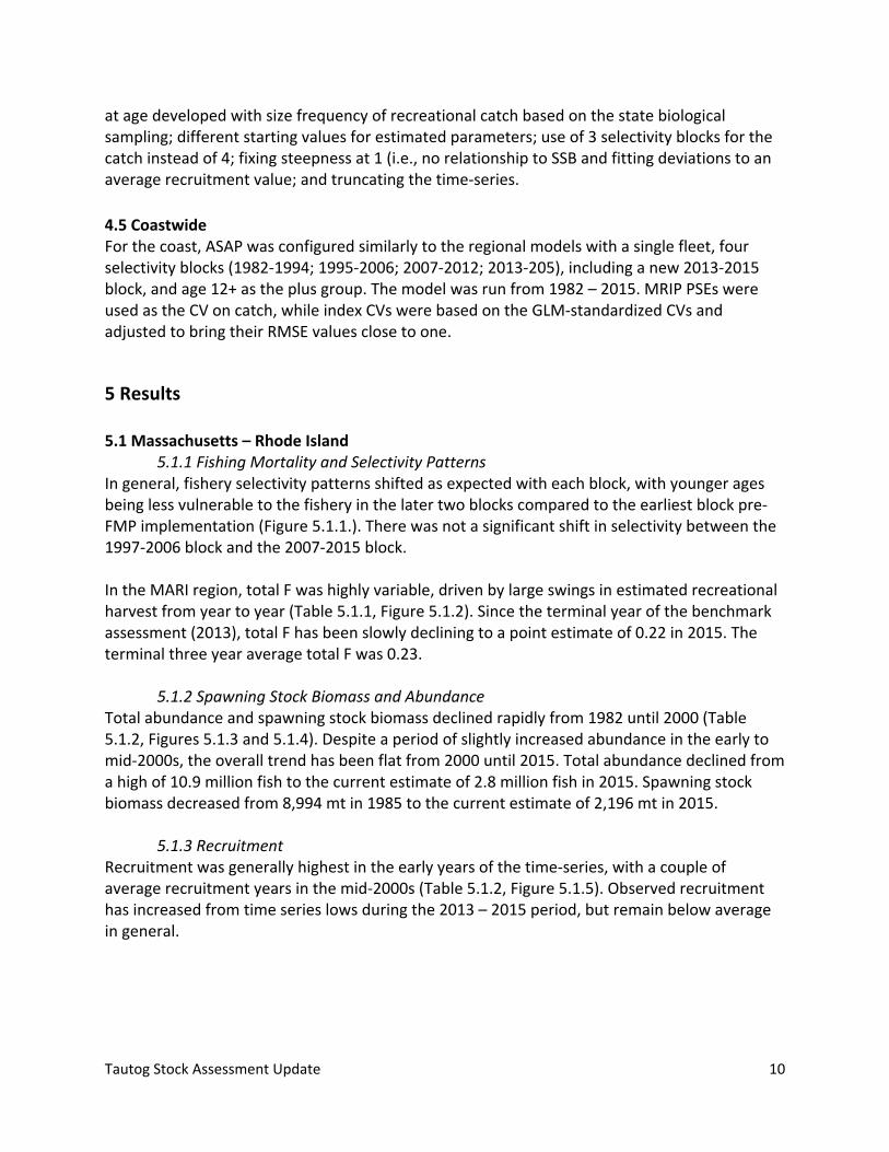
4.5 Coastwide For the coast, ASAP was configured similarly to the regional models with a single fleet, four selectivity blocks (1982‐1994; 1995‐2006; 2007‐2012; 2013‐205), including a new 2013‐2015 block, and age 12+ as the plus group. The model was run from 1982 – 2015. MRIP PSEs were used as the CV on catch, while index CVs were based on the GLM‐standardized CVs and adjusted to bring their RMSE values close to one.
5 Results
5.1 Massachusetts – Rhode Island 5.1.1 Fishing Mortality and Selectivity Patterns
In general, fishery selectivity patterns shifted as expected with each block, with younger ages being less vulnerable to the fishery in the later two blocks compared to the earliest block pre‐FMP implementation (Figure 5.1.1.). There was not a significant shift in selectivity between the 1997‐2006 block and the 2007‐2015 block. In the MARI region, total F was highly variable, driven by large swings in estimated recreational harvest from year to year (Table 5.1.1, Figure 5.1.2). Since the terminal year of the benchmark assessment (2013), total F has been slowly declining to a point estimate of 0.22 in 2015. The terminal three year average total F was 0.23.
5.1.2 Spawning Stock Biomass and Abundance Total abundance and spawning stock biomass declined rapidly from 1982 until 2000 (Table 5.1.2, Figures 5.1.3 and 5.1.4). Despite a period of slightly increased abundance in the early to mid‐2000s, the overall trend has been flat from 2000 until 2015. Total abundance declined from a high of 10.9 million fish to the current estimate of 2.8 million fish in 2015. Spawning stock biomass decreased from 8,994 mt in 1985 to the current estimate of 2,196 mt in 2015.
5.1.3 Recruitment Recruitment was generally highest in the early years of the time‐series, with a couple of average recruitment years in the mid‐2000s (Table 5.1.2, Figure 5.1.5). Observed recruitment has increased from time series lows during the 2013 – 2015 period, but remain below average in general.
Tautog Stock Assessment Update 11
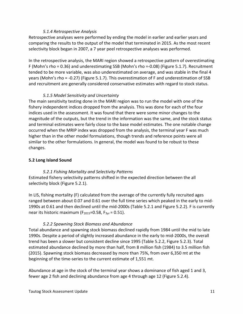
5.1.4 Retrospective Analysis Retrospective analyses were performed by ending the model in earlier and earlier years and comparing the results to the output of the model that terminated in 2015. As the most recent selectivity block began in 2007, a 7 year peel retrospective analyses was performed. In the retrospective analysis, the MARI region showed a retrospective pattern of overestimating F (Mohn’s rho = 0.36) and underestimating SSB (Mohn’s rho =‐0.08) (Figure 5.1.7). Recruitment tended to be more variable, was also underestimated on average, and was stable in the final 4 years (Mohn’s rho = ‐0.27) (Figure 5.1.7). This overestimation of F and underestimation of SSB and recruitment are generally considered conservative estimates with regard to stock status.
5.1.5 Model Sensitivity and Uncertainty The main sensitivity testing done in the MARI region was to run the model with one of the fishery independent indices dropped from the analysis. This was done for each of the four indices used in the assessment. It was found that there were some minor changes to the magnitude of the outputs, but the trend in the information was the same, and the stock status and terminal estimates were fairly close to the base model estimates. The one notable change occurred when the MRIP index was dropped from the analysis, the terminal year F was much higher than in the other model formulations, though trends and reference points were all similar to the other formulations. In general, the model was found to be robust to these changes.
5.2 Long Island Sound 5.2.1 Fishing Mortality and Selectivity Patterns
Estimated fishery selectivity patterns shifted in the expected direction between the all selectivity block (Figure 5.2.1). In LIS, fishing mortality (F) calculated from the average of the currently fully recruited ages ranged between about 0.07 and 0.61 over the full time series which peaked in the early to mid‐1990s at 0.61 and then declined until the mid‐2000s (Table 5.2.1 and Figure 5.2.2). F is currently near its historic maximum (F2015=0.58, F3yr = 0.51).
5.2.2 Spawning Stock Biomass and Abundance Total abundance and spawning stock biomass declined rapidly from 1984 until the mid to late 1990s. Despite a period of slightly increased abundance in the early to mid‐2000s, the overall trend has been a slower but consistent decline since 1995 (Table 5.2.2, Figure 5.2.3). Total estimated abundance declined by more than half, from 8 million fish (1984) to 3.5 million fish (2015). Spawning stock biomass decreased by more than 75%, from over 6,350 mt at the beginning of the time‐series to the current estimate of 1,551 mt. Abundance at age in the stock of the terminal year shows a dominance of fish aged 1 and 3, fewer age 2 fish and declining abundance from age 4 through age 12 (Figure 5.2.4).

Tautog Stock Assessment Update 12
5.2.3 Recruitment Recruitment was highest in the early years of the time series and again in 2013 and 2015 (Table 5.2.2, Figure 5.2.5. The two recent peaks in recruitment bracketed the lowest recruitment year on record. The stock‐recruitment relationship is shown in Figure 5.2.6. Steepness was estimated at 0.71. Estimates of steepness in the benchmark assessment were relatively robust to model configuration and there was good contrast in the stock size and recruitment levels over the time‐series, suggesting the relationship was reliable for BRP calculations.
5.2.4 Retrospective Analysis Retrospective analyses were performed by ending the model in progressively earlier years and comparing the results to the output of the model that terminated in 2015. In the retrospective analysis starting in 2012, F (Mohn’s rho = 0.303, Figure 5.2.7A) was underestimated in the last five years while SSB (Mohn’s rho = ‐ 0.147, Figure 5.2.7B) and recruitment (Mohn’s rho = ‐0.237, Figure 5.2.7C) were overestimated for the LIS region over the time series.
5.2.5. Model Sensitivity and Uncertainty For the LIS region, the LIS portion of the NY recreational harvest was revised for the years 2005‐2015 which resulted in a decrease of up to 45% of the total recreational harvest. Additionally, the LIS portion of the NY commercial harvest was revised for the years 2008‐2015, which resulted in a decrease harvest estimate of 20%. These estimates as based on numerous data streams and are a source of uncertainty. As the data is updated annually the model will be updated to reflect the most up‐to‐date estimates. Additionally, unquantified illegal live fish harvest from the region is not accounted for in the stock assessment, and this may be an influential mortality source.
5.3 New Jersey – New York Bight
5.3.1 Fishing Mortality and Selectivity Patterns Estimated fishery selectivity patterns shifted in the expected direction between the first and second selectivity blocks, but the model estimated an increase in selectivity at age for the third time block despite increased regulation. The reason for this is unknown but may be due to changes in data availability or sampling design. The 2012 size limit increase (via Addendum VI) shifted selectivity to the right as expected, with 50% selectivity between ages 5 and 6 (Figure 5.3.1). Consistent with previous assessments, including the 2015 benchmark, a three year moving average F was used to smooth the time series of fishing mortality (F). Fully exploited fishing mortality (F‐mult) shows high interannual variability, but suggests a cyclical pattern in exploitation over time, with ranges generally between 0.2 and 0.6 (Table 5.3.1, Figure 5.3.2). The declines in F are generally consistent with changes in regulations which often included increases in minimum size. F would then increase over the next few years as the fish grew into
Tautog Stock Assessment Update 13
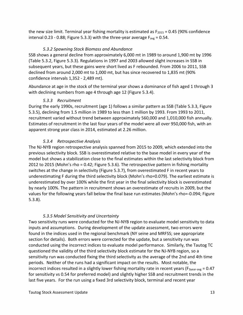
the new size limit. Terminal year fishing mortality is estimated as F2015 = 0.45 (90% confidence interval 0.23 ‐ 0.88; Figure 5.3.3) with the three‐year average Favg = 0.54.
5.3.2 Spawning Stock Biomass and Abundance SSB shows a general decline from approximately 6,000 mt in 1989 to around 1,900 mt by 1996 (Table 5.3.2, Figure 5.3.3). Regulations in 1997 and 2003 allowed slight increases in SSB in subsequent years, but these gains were short lived as F rebounded. From 2006 to 2011, SSB declined from around 2,000 mt to 1,000 mt, but has since recovered to 1,835 mt (90% confidence intervals 1,352 ‐ 2,489 mt).
Abundance at age in the stock of the terminal year shows a dominance of fish aged 1 through 3 with declining numbers from age 4 through age 12 (Figure 5.3.4).
5.3.3 Recruitment During the early 1990s, recruitment (age 1) follows a similar pattern as SSB (Table 5.3.3, Figure 5.3.5), declining from 1.5 million in 1989 to less than 1 million by 1993. From 1993 to 2011, recruitment varied without trend between approximately 560,000 and 1,010,000 fish annually. Estimates of recruitment in the last four years of the model were all over 950,000 fish, with an apparent strong year class in 2014, estimated at 2.26 million.
5.3.4 Retrospective Analysis The NJ‐NYB region retrospective analysis spanned from 2015 to 2009, which extended into the previous selectivity block. SSB is overestimated relative to the base model in every year of the model but shows a stabilization close to the final estimates within the last selectivity block from 2012 to 2015 (Mohn’s rho = 0.42; Figure 5.3.6). The retrospective pattern in fishing mortality switches at the change in selectivity (Figure 5.3.7), from overestimated F in recent years to underestimating F during the third selectivity block (Mohn’s rho=0.079). The earliest estimate is underestimated by over 100% while the first year in the final selectivity block is overestimated by nearly 100%. The pattern in recruitment shows an overestimate of recruits in 2009, but the values for the following years fall below the final base run estimates (Mohn’s rho=‐0.094; Figure 5.3.8).
5.3.5 Model Sensitivity and Uncertainty Two sensitivity runs were conducted for the NJ‐NYB region to evaluate model sensitivity to data inputs and assumptions. During development of the update assessment, two errors were found in the indices used in the regional benchmark (NY seine and MRFSS; see appropriate section for details). Both errors were corrected for the update, but a sensitivity run was conducted using the incorrect indices to evaluate model performance. Similarly, the Tautog TC questioned the validity of the third selectivity block estimate for the NJ‐NYB region, so a sensitivity run was conducted fixing the third selectivity as the average of the 2nd and 4th time periods. Neither of the runs had a significant impact on the results. Most notable, the incorrect indices resulted in a slightly lower fishing mortality rate in recent years (F3year‐avg = 0.47 for sensitivity vs 0.54 for preferred model) and slightly higher SSB and recruitment trends in the last five years. For the run using a fixed 3rd selectivity block, terminal and recent year
Tautog Stock Assessment Update 14
estimates were nearly identical to the preferred run, but fishing mortality for the years of that selectivity block (2004‐2011) increased over the preferred run. This is consistent with the retrospective pattern which indicates F was underestimated in those years. F reference points were consistent among the runs, as was stock status with respect to F.
5.4 DelMarVa 5.4.1 Fishing Mortality and Selectivity Patterns
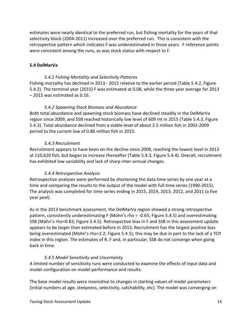
Fishing mortality has declined in 2013 ‐ 2015 relative to the earlier period (Table 5.4.2, Figure 5.4.2). The terminal year (2015) F was estimated at 0.08, while the three year average for 2013 – 2015 was estimated as 0.16.
5.4.2 Spawning Stock Biomass and Abundance Both total abundance and spawning stock biomass have declined steadily in the DelMarVa region since 2009, and SSB reached historically low level of 609 mt in 2015 (Table 5.4.3, Figure 5.4.3). Total abundance declined from a stable level of about 2.5 million fish in 2002‐2009 period to the current low of 0.86 million fish in 2015.
5.4.3 Recruitment Recruitment appears to have been on the decline since 2009, reaching the lowest level in 2013 at 110,620 fish, but began to increase thereafter (Table 5.4.3, Figure 5.4.4). Overall, recruitment has exhibited low variability and lack of sharp inter‐annual changes.
5.4.4 Retrospective Analysis Retrospective analyses were performed by shortening the data time series by one year at a time and comparing the results to the output of the model with full time series (1990‐2015). The analysis was completed for time series ending in 2015, 2014, 2013, 2012, and 2011 (a five year peel). As in the 2013 benchmark assessment, the DelMarVa region showed a strong retrospective pattern, consistently underestimating F (Mohn’s rho = ‐0.65; Figure 5.4.5) and overestimating SSB (Mohn’s rho=0.83; Figure 5.4.5). Retrospective bias in F and SSB in this assessment update appears to be larger than estimated before in 2013. Recruitment has the largest positive bias being overestimated (Mohn’s rho=2.2; Figure 5.4.5); this may be due in part to the lack of a YOY index in this region. The estimates of R, F and, in particular, SSB do not converge when going back in time.
5.4.5 Model Sensitivity and Uncertainty A limited number of sensitivity runs were conducted to examine the effects of input data and model configuration on model performance and results. The base model results were insensitive to changes in starting values of model parameters (initial numbers at age, steepness, selectivity, catchability, etc). The model was converging on
Tautog Stock Assessment Update 15
the same parameters estimates, within a range of initial starting values, indicating stability of model solution. Fixing steepness parameter at 1, thus assuming no stock recruitment relationship, had very little effect on the final model results. The model was also insensitive to the introduction of the additional, 4th selectivity block covering 2012‐2015 period. Estimates of F and SSB were nearly identical to those from the model run with three selectivity blocks, where the third block covered the period of 2007 ‐2012. Forcing the model to fit the catch information exactly (by reducing catch CVs to a very small value) is one of the few outcomes where the results are rather different – the SSB estimates appear to be significantly larger, particularly in the most recent period (SSB in 2015 is 57% higher than the base run), while the fishing mortality is significantly lower (55% of the base run estimate in 2015. Truncation of the time series (starting the model in 1995 rather than in 1990) leads to a slightly lower SSB and higher F estimates relative to the base run. Addition of NJ trawl index as the geographically nearest fishery independent survey resulted in very small changes in SSB estimates, but slightly higher F relative to the base run. Overall, the model estimates appear to be stable and not sensitive to changes explored in various sensitivity runs.
5.5 Coastwide 5.5.1 Fishing Mortality and Selectivity Patterns
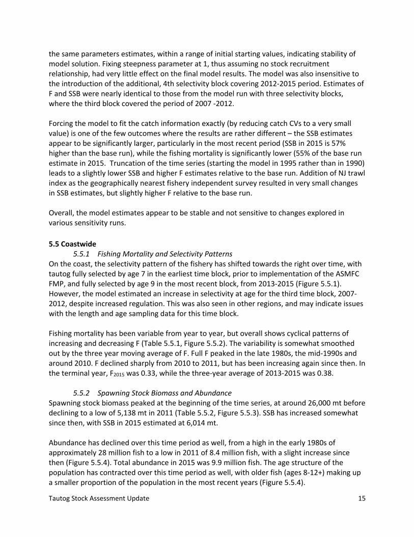
On the coast, the selectivity pattern of the fishery has shifted towards the right over time, with tautog fully selected by age 7 in the earliest time block, prior to implementation of the ASMFC FMP, and fully selected by age 9 in the most recent block, from 2013‐2015 (Figure 5.5.1). However, the model estimated an increase in selectivity at age for the third time block, 2007‐2012, despite increased regulation. This was also seen in other regions, and may indicate issues with the length and age sampling data for this time block. Fishing mortality has been variable from year to year, but overall shows cyclical patterns of increasing and decreasing F (Table 5.5.1, Figure 5.5.2). The variability is somewhat smoothed out by the three year moving average of F. Full F peaked in the late 1980s, the mid‐1990s and around 2010. F declined sharply from 2010 to 2011, but has been increasing again since then. In the terminal year, F2015 was 0.33, while the three‐year average of 2013‐2015 was 0.38.
5.5.2 Spawning Stock Biomass and Abundance Spawning stock biomass peaked at the beginning of the time series, at around 26,000 mt before declining to a low of 5,138 mt in 2011 (Table 5.5.2, Figure 5.5.3). SSB has increased somewhat since then, with SSB in 2015 estimated at 6,014 mt. Abundance has declined over this time period as well, from a high in the early 1980s of approximately 28 million fish to a low in 2011 of 8.4 million fish, with a slight increase since then (Figure 5.5.4). Total abundance in 2015 was 9.9 million fish. The age structure of the population has contracted over this time period as well, with older fish (ages 8‐12+) making up a smaller proportion of the population in the most recent years (Figure 5.5.4).
Tautog Stock Assessment Update 16
5.5.3 Recruitment
Recruitment has declined since the beginning of the time series, from approximately 5.9 million age‐1 fish in 1982 to a low of 1.75 million fish in 1996 (Table 5.5.2, Figure 5.5.5). Recruitment has fluctuated around a mean of 2.2 million fish since then. Recruitment in 2015 was estimated at 2.1 million fish, slightly below the time‐series mean of 2.75 million fish. The spawner‐recruit relationship is shown in Figure 5.5.6. Steepness was estimated at 0.55, indicating a moderately productive species.
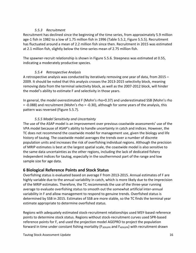
5.5.4 Retrospective Analysis A retrospective analysis was conducted by iteratively removing one year of data, from 2015 – 2009. It should be noted that this analysis crosses the 2013‐2015 selectivity block, meaning removing data from the terminal selectivity block, as well as the 2007‐2012 block, will hinder the model’s ability to estimate F and selectivity in those years. In general, the model overestimated F (Mohn’s rho=0.37) and underestimated SSB (Mohn’s rho = ‐0.088) and recruitment (Mohn’s rho = ‐0.30), although for some years of the analysis, this pattern was reversed (Figure 5.5.7).
5.5.5 Model Sensitivity and Uncertainty The use of the ASAP model is an improvement over previous coastwide assessments’ use of the VPA model because of ASAP’s ability to handle uncertainty in catch and indices. However, the TC does not recommend the coastwide model for management use, given the biology and life history of tautog. The coastwide model averages the trends over a number of discrete population units and increases the risk of overfishing individual regions. Although the precision of MRIP estimates is best at the largest spatial scale, the coastwide model is also sensitive to the same data uncertainties as the other regions, including the lack of dedicated fishery independent indices for tautog, especially in the southernmost part of the range and low sample size for age data.
6 Biological Reference Points and Stock Status Overfishing status is evaluated based on average F from 2013‐2015. Annual estimates of F are highly variable due to the annual variability in catch, which is more likely due to the imprecision of the MRIP estimates. Therefore, the TC recommends the use of the three‐year running average to evaluate overfishing status to smooth out the somewhat artificial inter‐annual variability in F and allow management to respond to genuine trends. Overfished status is determined by SSB in 2015. Estimates of SSB are more stable, so the TC finds the terminal year estimate appropriate to determine overfished status. Regions with adequately estimated stock‐recruitment relationships used MSY‐based reference points to determine stock status. Regions without stock‐recruitment curves used SPR‐based reference points for F, and used the projection model AGEPRO to project the population forward in time under constant fishing mortality (F30%SPR and F40%SPR) with recruitment drawn
Tautog Stock Assessment Update 17
from the model estimated time‐series of observed recruitment to develop an estimate of the long‐term equilibrium SSB associated with those fishing mortality reference points.
6.1 Massachusetts‐Rhode Island Estimated steepness of the MARI regional model was deemed credible by the TC during the benchmark assessment, and the TC therefore recommends MSY‐based benchmarks for this region. The steepness parameter was similar to that estimated during the benchmark (steepness = 0.45), therefore MSY reference points were used for this update to be consistent with the benchmark recommendations. Because there was considerable discussion by the TC regarding the utility of the different reference point models, SPR‐based reference points are also provided for the MARI region.
6.1.1 Overfishing Status Ftarget was defined as FMSY with Fthreshold set at the F value necessary to achieve the SSB threshold, 75%SSBMSY, in the long term. These two reference points are Ftarget = 0.14 and Fthreshold = 0.28. The three year average of F for 2013‐2015 is 0.23. This value is below the threshold, indicating overfishing is not occurring, but it is still above the target (Figure 6.1.1). For SPR estimates, the 3‐year average value of F3yr = 0.23 was below both FTarget = 0.28 and Fthreshold = 0.49 (Figure 6.1.3), thus indicating by the SPR reference points that this stock is not experiencing overfishing and is at a fishing mortality rate that is below the target.
6.1.2 Overfished Status For the MARI region, SSBtarget was defined as SSBMSY = 3,631 mt and SSBthreshold was defined as 75% of SSBMSY = 2,723 mt. SSB2015 was estimated at 2,196 mt, below both the target and the threshold, indicating the stock is overfished (Figure 6.1.2). For SPR estimates, the point estimate of SSB2015 = 2,196 mt is below the SSBTarget = 2,684 mt but is above the SSBthreshold = 2,004 mt (Figure 6.1.4), thus indicating that the stock is not overfished but is not yet rebuilt to the SSB target.
6.2 Long Island Sound
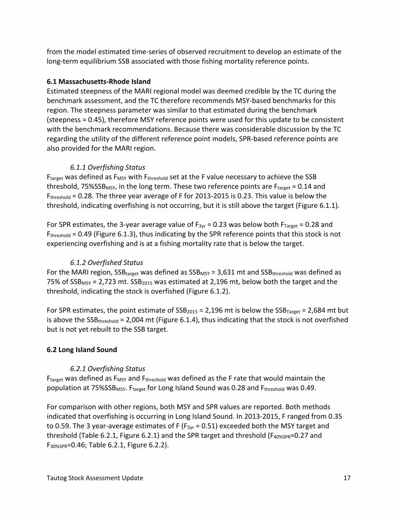
6.2.1 Overfishing Status Ftarget was defined as FMSY and Fthreshold was defined as the F rate that would maintain the population at 75%SSBMSY. Ftarget for Long Island Sound was 0.28 and Fthreshold was 0.49. For comparison with other regions, both MSY and SPR values are reported. Both methods indicated that overfishing is occurring in Long Island Sound. In 2013‐2015, F ranged from 0.35 to 0.59. The 3 year‐average estimates of F (F3yr = 0.51) exceeded both the MSY target and threshold (Table 6.2.1, Figure 6.2.1) and the SPR target and threshold (F40%SPR=0.27 and F30%SPR=0.46; Table 6.2.1, Figure 6.2.2).
Tautog Stock Assessment Update 18
6.2.2 Overfished Status The ASAP model runs using both MSY and SPR methods indicated that the tautog stock is overfished in Long Island Sound. SSB2015 (1,603 mt, Table 6.2.1, Figure 6.2.1) is below MSY target and threshold (SSBMSY = 2,865 mt and SSB75%MSY = 2,148 mt) as well as SPR target and threshold (SSB40% = 2,980 mt and SSB30%SPR = 2,238 mt; Table 6.2.1, Figure 6.2.2).
6.3 New Jersey – New York Bight
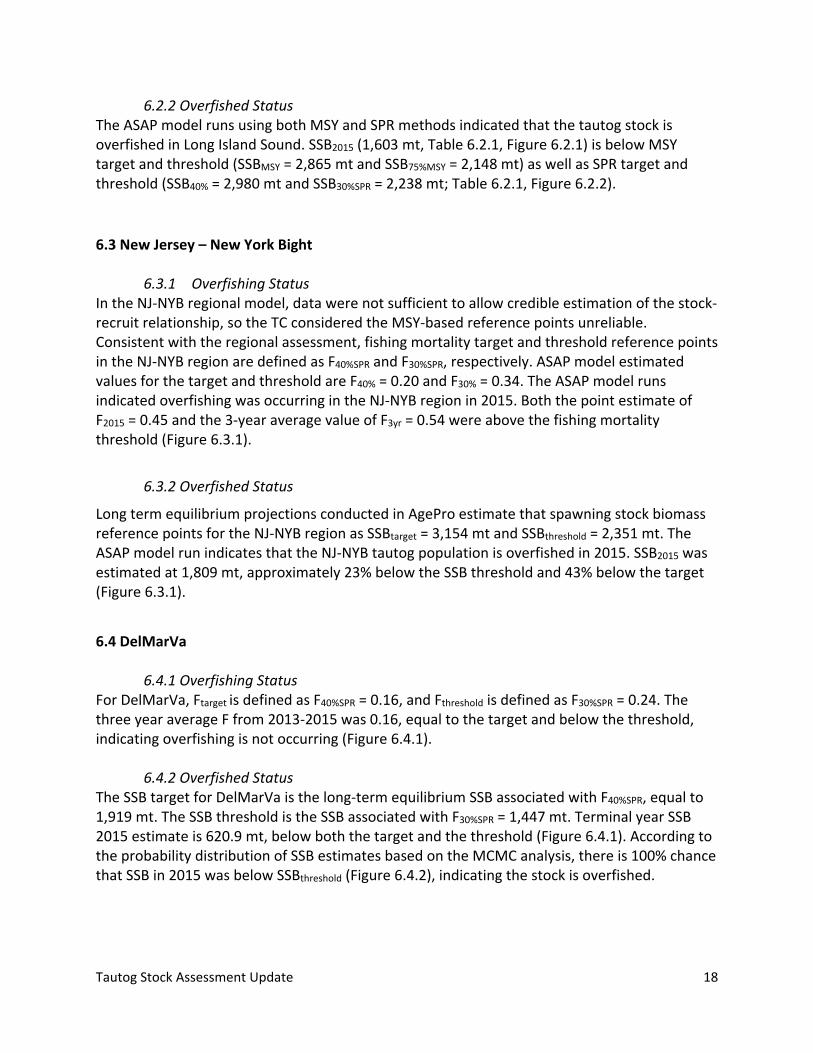
6.3.1 Overfishing Status In the NJ‐NYB regional model, data were not sufficient to allow credible estimation of the stock‐recruit relationship, so the TC considered the MSY‐based reference points unreliable. Consistent with the regional assessment, fishing mortality target and threshold reference points in the NJ‐NYB region are defined as F40%SPR and F30%SPR, respectively. ASAP model estimated values for the target and threshold are F40% = 0.20 and F30% = 0.34. The ASAP model runs indicated overfishing was occurring in the NJ‐NYB region in 2015. Both the point estimate of F2015 = 0.45 and the 3‐year average value of F3yr = 0.54 were above the fishing mortality threshold (Figure 6.3.1).
6.3.2 Overfished Status
Long term equilibrium projections conducted in AgePro estimate that spawning stock biomass reference points for the NJ‐NYB region as SSBtarget = 3,154 mt and SSBthreshold = 2,351 mt. The ASAP model run indicates that the NJ‐NYB tautog population is overfished in 2015. SSB2015 was estimated at 1,809 mt, approximately 23% below the SSB threshold and 43% below the target (Figure 6.3.1).
6.4 DelMarVa
6.4.1 Overfishing Status For DelMarVa, Ftarget is defined as F40%SPR = 0.16, and Fthreshold is defined as F30%SPR = 0.24. The three year average F from 2013‐2015 was 0.16, equal to the target and below the threshold, indicating overfishing is not occurring (Figure 6.4.1).
6.4.2 Overfished Status The SSB target for DelMarVa is the long‐term equilibrium SSB associated with F40%SPR, equal to 1,919 mt. The SSB threshold is the SSB associated with F30%SPR = 1,447 mt. Terminal year SSB 2015 estimate is 620.9 mt, below both the target and the threshold (Figure 6.4.1). According to the probability distribution of SSB estimates based on the MCMC analysis, there is 100% chance that SSB in 2015 was below SSBthreshold (Figure 6.4.2), indicating the stock is overfished.
Tautog Stock Assessment Update 19
6.5 Coastwide
6.5.1 Overfishing Status For the coast, Ftarget was defined as FMSY and Fthreshold was defined as the F rate that would maintain the population at 75%SSBMSY. FMSY for the coastwide population was 0.17 and F75%SSB was 0.24. The 2013‐2015 average F was 0.38, above both the MSY‐based target and the threshold, indicating overfishing was occurring (Figure 6.5.1). For comparison, F30%SPR was 0.43 and F40% was 0.25. The 2013‐2015 average F was between those two values (Figure 6.5.2).
6.5.2 Overfished Status SSBtarget was defined as SSBMSY, estimated at 14,944 mt, and SSBthreshold was 75% of SSBMSY, or 11,208 mt. In 2015, SSB was 6,014 mt, below both the target and the threshold, indicating the stock was overfished (Figure 6.5.1). For comparison, the SSB30% associated with F30%SPR was 7,091 mt and the SSB40% associated with F40%SPR was 9,448 mt. SSB in 2015 was below both of these values as well (Figure 6.5.2).
7 Projections AgePro (v. 4.2, NOAA Fisheries Toolbox), was used to conduct short term (2016‐2020) projection scenarios to determine constant harvest levels that would result in 50% chance and 70% chance of achieving the regional F targets in 2020, as well as to project trends under status quo removals. Biological parameters (maturity, M, weights at age) for the projection model were the same used in the ASAP population model, with the exception that projection catch weights at age were set equal to the average catch weight at age in the most recent selectivity block. The model assumed empirical recruitment drawn from the ASAP estimated observed recruitment vector for SPR reference points, and Beverton and Holt recruitment with lognormal error using parameter estimated by ASAP for MSY‐based reference points. Fishery selectivity was input as that estimated by ASAP in the most recent selectivity period. Harvest for 2016 and 2017 were assumed equal to the most recent three year average harvest. An iterative process was used to determine a constant harvest rate in 2018‐2020 that resulted in 50% and 70% probabilities of achieving Ftarget.
7.1 Massachusetts – Rhode Island Probability estimates of achieving MSY reference points (FMSYTarget and SSB75%MSY) and SPR reference points (F40%SPR and SSB30%) in 3 years from short term projections (2017 through 2020) are shown in Table 7.1.1 and Figures 7.1.1 and 7.1.2. Under status quo conditions (2013‐2015 average landings of 390 mt), using MSY reference points there is 0% probability of achieving FTarget and 0% probability of reaching SSBThreshold (Table 7.1.1, Figure 7.1.1). Similarly, under status quo conditions, using SPR reference points there is 0% probability of achieving F40% but a 4.1% probability of reaching SSB30%SPR (Table 7.1.1, Figure 7.1.2).
Tautog Stock Assessment Update 20
Reducing landings to 151 mt (approximately 55% of 2015 landings) and using MSY reference points results in a 50% probability of achieving Ftarget and 2.2% probability of achieving SSBThreshold (Table 7.1.1, Figure 7.1.3). With MSY reference points, landings of 148 mt (a 56% reduction from 2015 landings) results in a 70% probability of achieving Ftarget and 2.3% probability of achieving SSBThreshold by 2020 (Table 7.1.1, Figure 7.1.4). Using SPR reference points, a harvest reduction of 24% from 2015 landings to 257 mt results in a 50% probability of achieving F40%SPR and 23.2% probability of achieving SSB30%SPR (Table 7.1.1, Figure 7.1.5). Annual landings of 253 mt (a 25% reduction from 2015 levels) results in a 70% probability of achieving F40%SPR and 24.3% probability of achieving SSB30%SPR (Table 7.1.1, Figure 7.1.6).
7.2. Long Island Sound Under status quo conditions (2013‐2015 average landings of 500 mt), using MSY reference points, there is 1.7% probability of achieving FTarget and 0.6% probability of reaching SSBThreshold (Table 7.2.1, Figure 7.2.1). Similarly, under status quo conditions, using SPR reference points there is 0% probability of achieving FTarget and 0.6% probability of reaching SSBThreshold (Table 7.2.1). Reducing landings to 264 mt (a 39% reduction from 2015 levels) and using MSY reference points results in a 50% probability of achieving Ftarget and 34% probability of achieving SSBThreshold (Table 7.2.1, Figure 7.2.2). With MSY reference points, landings of 229 mt (a 47% reduction from 2015 levels) results in a 70% probability of achieving Ftarget and 40% probability of achieving SSBThreshold by 2020 (Table 7.2.1, Figure 7.2.3). Using SPR reference points, a harvest reduction of 41% (to 255 mt) results in a 50% probability of achieving F40%SPR and 28% probability of achieving SSB30%SPR (Table 7.2.1, Figure 7.2.4). Annual landings of 229 mt (47% reduction from 2015) results in a 70% probability of achieving the SPR F40%SPR and 33% probability of achieving SSB30%SPR (Table 7.2.1, Figure 7.2.5).
7.3 New Jersey – New York Bight Probability estimates of achieving FTarget and SSBThreshold in 2020 years from short term projections (2016 through 2020) are shown in Table 7.3.1 and Figures 7.3.1 – 7.3.3. Under status quo conditions (2013‐2015 average landings of 461 mt), there is a 45% probability of achieving FTarget and an 85% probability of being at or above SSBthreshold in 2020 (Table 7.3.1, Figure 7.3.1). Constant harvest of 450 mt (a 2.3% reduction from the 2013‐2015 average but a 35% increase from 2015 levels) results in a 50% probability of achieving Ftarget and 86% probability of being at or above SSBthreshold (Table 7.3.1, Figure 7.3.2). Annual landings of 410 mt (an 11% reduction from the 3‐year average and a 23% increase from 2015 levels), provides a 70% probability of achieving Ftarget and an 88% probability of being at or above SSBthreshold (Table 7.3.1, Figure 7.3.3).
Tautog Stock Assessment Update 21
7.4 DelMarVa If the constant catch of 77.0 mt was maintained during 2016‐2020 (status quo scenario), the probability of the fully‐recruited F being at or below the F target by the year 2020 is expected to be 99.64%, while the probability of SSB being at or above SSB threshold is 18.15 % (Table 7.4.1, Figure 7.4.1). Fishing mortality will rise to 0.13 in 2016 and will decline thereafter to F=0.076 by 2020 (Figure 7.4.1). SSB is projected to grow but the median will reach only 1320.5 mt (Figure 7.4.1). A 50% probability for F being at or below Fthreshold by year 2020 can be achieved by maintaining total annual removals at 136 mt, an increase from both the 3 year average and 2015 levels; however, this results in a very low chance (9.9%) of SSB reaching the SSB threshold (Table 7.4.1; Figure 7.4.2). A 70% chance of F being at or below Fthreshold by year 2020 requires to maintain annual removals in 2018‐2020 at 125 mt, but the chance for SSB reaching SSB target is only 11.9% (Table 7.4.1; Figure 7.4.3).
7.5 Coastwide Under status quo harvest (the average of the last three years, 1,270 mt), there is zero probability of attaining the Ftarget in 2020, and less than 1% probability of being at or above the SSB threshold (Table 7.5.1, Figure 7.5.1). To have a 50% chance of being at or below the F target in 2020, harvest for 2018‐2020 needs to be reduced to 737 mt, an 18.5% reduction from 2015 harvest (Table 7.5.1, Figure 7.5.2). This results in a 0.9% chance that SSB will be at or above the threshold in 2020 (Figure 7.5.2). To have a 70% chance of being at or below the F target in 2020, harvest for 2017‐2020 needs to be reduced to 682 mt, a 24.6% reduction from 2015 harvest (Table 7.5.1, Figure 7.5.3). This results in a 1% chance that SSB will be at or above the threshold in 2020 (Figure 7.5.3).
These calculations were done using the MSY‐based target and threshold reference points. Status quo harvest results in a 2.7% chance that F will be at or below F40%SPR in 2020, and a 29.4% chance that SSB will be at or above SSB30% (Table 7.5.1, Figure 7.5.4). To have a 50% chance of achieving F40%SPR, harvest in 2018‐2020 needs to be 968 mt, a 23.8% reduction from the 2013‐2015 average harvest, but a 7% increase from 2015 harvest (Table 7.5.1, Figure 7.5.5). This results in a 50.2% probability of SSB being at or above SSB30% (Figure 7.5.5). To have a 70% chance of being at or below F40%SPR, harvest in 2018‐2020 needs to be reduced to 895 mt, a reduction of 1% from 2015 harvest levels and a reduction of 29.5% from the 2013‐

Tautog Stock Assessment Update 22
2015 average harvest (Table 7.5.1, Figure 7.5.6). This results in a 55.3% probability of SSB being above SSB30% (Figure 7.5.5).
8 Research Recommendations For all regions, the TC recommends expanding the biological sampling of catch and discards, both commercial and recreational, as well as increased MRIP sampling levels to improve estimates of total catch, as high priorities to improve the assessment. In addition, establishing standardized multi‐state fishery independent surveys using gear appropriate for structure‐oriented species (e.g., fish pots or traps) is a high priority to improve the quality of fishery independent abundance information for the assessment. Genetic analyses with up‐to‐date methodologies could also help refine regional boundaries. Better monitoring of illegal harvest to develop more accurate estimates of these removals and improve compliance would also be useful to both the assessment and management of this species.
9 Literature Cited
Atlantic States Marine Fisheries Commission. 1996. Fisheries Management Plan for Tautog. ASMFC, Washington, DC.
Atlantic States Marine Fisheries Commission. 2015. Tautog benchmark stock assessment.
Arlington, VA. Atlantic States Marine Fisheries Commission. 2016. Tautog regional stock assessment: Long
Island Sound and New Jersey‐New York Bight. Arlington, VA.
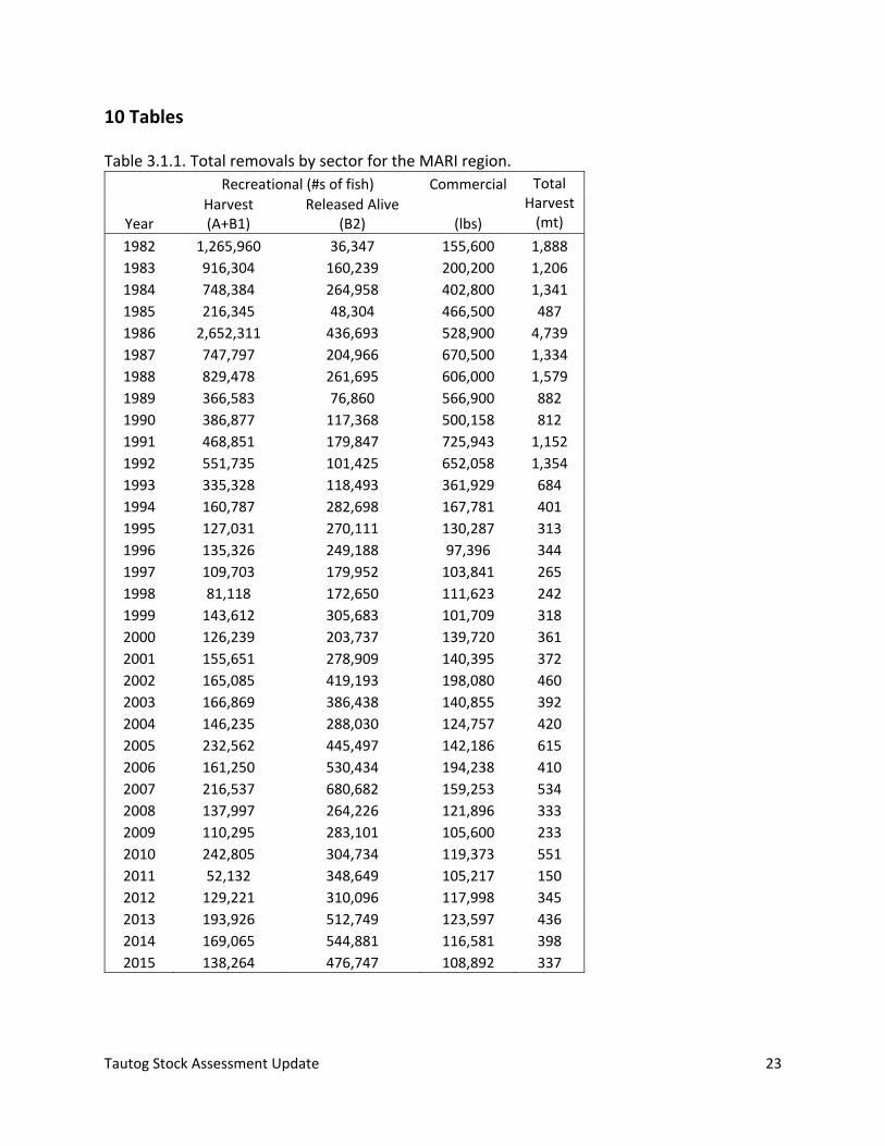
Tautog Stock Assessment Update 23
10 Tables Table 3.1.1. Total removals by sector for the MARI region.
Recreational (#s of fish) Commercial Total Harvest (mt) Year
Harvest (A+B1)
Released Alive (B2) (lbs)
1982 1,265,960 36,347 155,600 1,888
1983 916,304 160,239 200,200 1,206
1984 748,384 264,958 402,800 1,341
1985 216,345 48,304 466,500 487
1986 2,652,311 436,693 528,900 4,739
1987 747,797 204,966 670,500 1,334
1988 829,478 261,695 606,000 1,579
1989 366,583 76,860 566,900 882
1990 386,877 117,368 500,158 812
1991 468,851 179,847 725,943 1,152
1992 551,735 101,425 652,058 1,354
1993 335,328 118,493 361,929 684
1994 160,787 282,698 167,781 401
1995 127,031 270,111 130,287 313
1996 135,326 249,188 97,396 344
1997 109,703 179,952 103,841 265
1998 81,118 172,650 111,623 242
1999 143,612 305,683 101,709 318
2000 126,239 203,737 139,720 361
2001 155,651 278,909 140,395 372
2002 165,085 419,193 198,080 460
2003 166,869 386,438 140,855 392
2004 146,235 288,030 124,757 420
2005 232,562 445,497 142,186 615
2006 161,250 530,434 194,238 410
2007 216,537 680,682 159,253 534
2008 137,997 264,226 121,896 333
2009 110,295 283,101 105,600 233
2010 242,805 304,734 119,373 551
2011 52,132 348,649 105,217 150
2012 129,221 310,096 117,998 345
2013 193,926 512,749 123,597 436
2014 169,065 544,881 116,581 398
2015 138,264 476,747 108,892 337
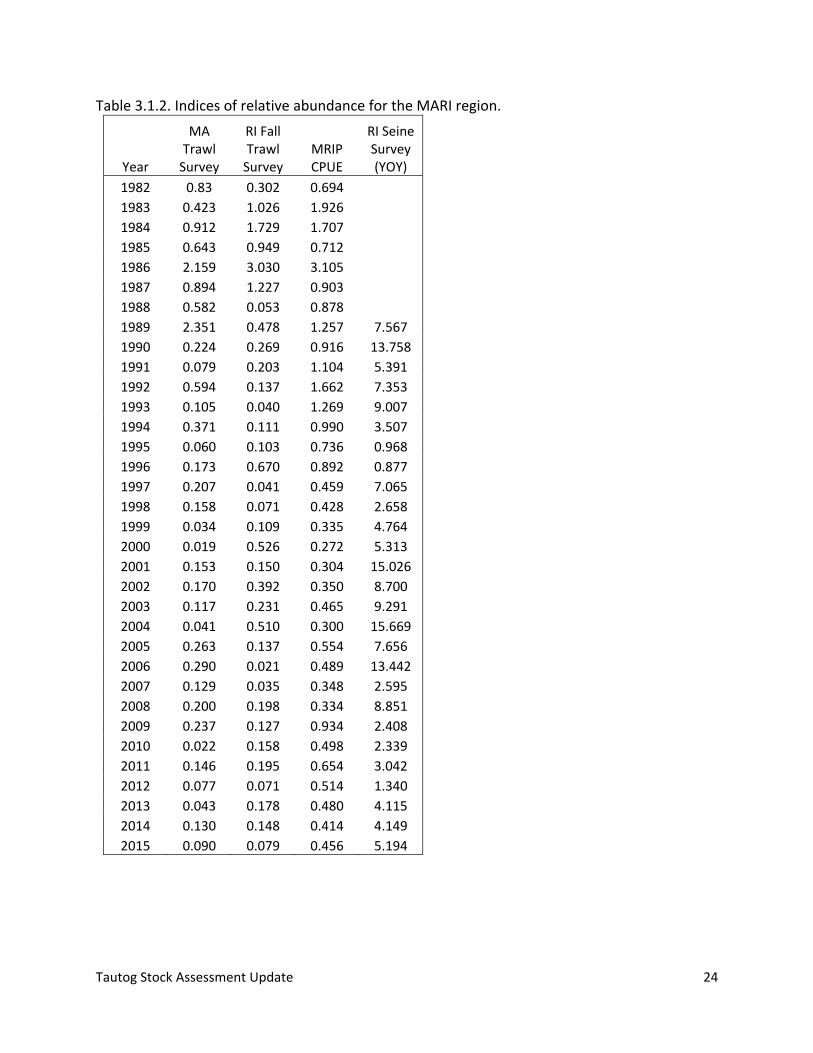
Tautog Stock Assessment Update 24
Table 3.1.2. Indices of relative abundance for the MARI region.
Year
MA Trawl Survey
RI Fall Trawl Survey
MRIP CPUE
RI Seine Survey (YOY)
1982 0.83 0.302 0.694
1983 0.423 1.026 1.926
1984 0.912 1.729 1.707
1985 0.643 0.949 0.712
1986 2.159 3.030 3.105
1987 0.894 1.227 0.903
1988 0.582 0.053 0.878
1989 2.351 0.478 1.257 7.567
1990 0.224 0.269 0.916 13.758
1991 0.079 0.203 1.104 5.391
1992 0.594 0.137 1.662 7.353
1993 0.105 0.040 1.269 9.007
1994 0.371 0.111 0.990 3.507
1995 0.060 0.103 0.736 0.968
1996 0.173 0.670 0.892 0.877
1997 0.207 0.041 0.459 7.065
1998 0.158 0.071 0.428 2.658
1999 0.034 0.109 0.335 4.764
2000 0.019 0.526 0.272 5.313
2001 0.153 0.150 0.304 15.026
2002 0.170 0.392 0.350 8.700
2003 0.117 0.231 0.465 9.291
2004 0.041 0.510 0.300 15.669
2005 0.263 0.137 0.554 7.656
2006 0.290 0.021 0.489 13.442
2007 0.129 0.035 0.348 2.595
2008 0.200 0.198 0.334 8.851
2009 0.237 0.127 0.934 2.408
2010 0.022 0.158 0.498 2.339
2011 0.146 0.195 0.654 3.042
2012 0.077 0.071 0.514 1.340
2013 0.043 0.178 0.480 4.115
2014 0.130 0.148 0.414 4.149
2015 0.090 0.079 0.456 5.194
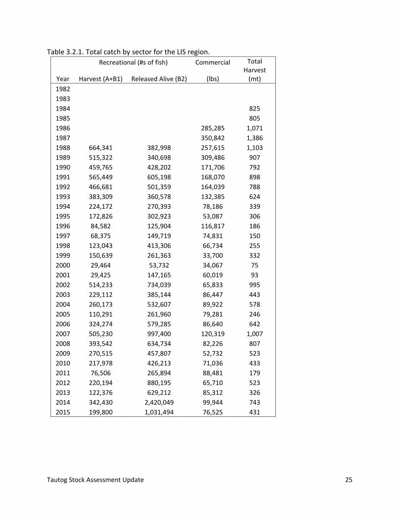
Tautog Stock Assessment Update 25
Table 3.2.1. Total catch by sector for the LIS region.
Recreational (#s of fish) Commercial Total Harvest (mt)Year Harvest (A+B1) Released Alive (B2) (lbs)
1982
1983
1984 825
1985 805
1986 285,285 1,071
1987 350,842 1,386
1988 664,341 382,998 257,615 1,103
1989 515,322 340,698 309,486 907
1990 459,765 428,202 171,706 792
1991 565,449 605,198 168,070 898
1992 466,681 501,359 164,039 788
1993 383,309 360,578 132,385 624
1994 224,172 270,393 78,186 339
1995 172,826 302,923 53,087 306
1996 84,582 125,904 116,817 186
1997 68,375 149,719 74,831 150
1998 123,043 413,306 66,734 255
1999 150,639 261,363 33,700 332
2000 29,464 53,732 34,067 75
2001 29,425 147,165 60,019 93
2002 514,233 734,039 65,833 995
2003 229,112 385,144 86,447 443
2004 260,173 532,607 89,922 578
2005 110,291 261,960 79,281 246
2006 324,274 579,285 86,640 642
2007 505,230 997,400 120,319 1,007
2008 393,542 634,734 82,226 807
2009 270,515 457,807 52,732 523
2010 217,978 426,213 71,036 433
2011 76,506 265,894 88,481 179
2012 220,194 880,195 65,710 523
2013 122,376 629,212 85,312 326
2014 342,430 2,420,049 99,944 743
2015 199,800 1,031,494 76,525 431
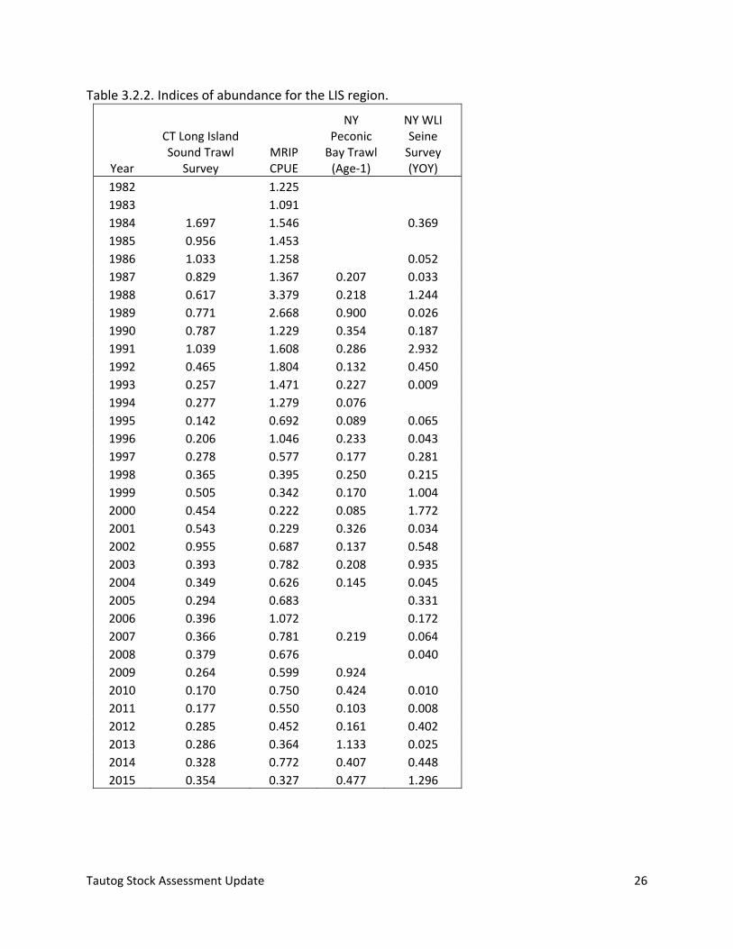
Tautog Stock Assessment Update 26
Table 3.2.2. Indices of abundance for the LIS region.
Year
CT Long Island Sound Trawl
Survey MRIP CPUE
NY Peconic Bay Trawl (Age‐1)
NY WLI Seine Survey (YOY)
1982 1.225
1983 1.091
1984 1.697 1.546 0.369
1985 0.956 1.453
1986 1.033 1.258 0.052
1987 0.829 1.367 0.207 0.033
1988 0.617 3.379 0.218 1.244
1989 0.771 2.668 0.900 0.026
1990 0.787 1.229 0.354 0.187
1991 1.039 1.608 0.286 2.932
1992 0.465 1.804 0.132 0.450
1993 0.257 1.471 0.227 0.009
1994 0.277 1.279 0.076
1995 0.142 0.692 0.089 0.065
1996 0.206 1.046 0.233 0.043
1997 0.278 0.577 0.177 0.281
1998 0.365 0.395 0.250 0.215
1999 0.505 0.342 0.170 1.004
2000 0.454 0.222 0.085 1.772
2001 0.543 0.229 0.326 0.034
2002 0.955 0.687 0.137 0.548
2003 0.393 0.782 0.208 0.935
2004 0.349 0.626 0.145 0.045
2005 0.294 0.683 0.331
2006 0.396 1.072 0.172
2007 0.366 0.781 0.219 0.064
2008 0.379 0.676 0.040
2009 0.264 0.599 0.924
2010 0.170 0.750 0.424 0.010
2011 0.177 0.550 0.103 0.008
2012 0.285 0.452 0.161 0.402
2013 0.286 0.364 1.133 0.025
2014 0.328 0.772 0.407 0.448
2015 0.354 0.327 0.477 1.296
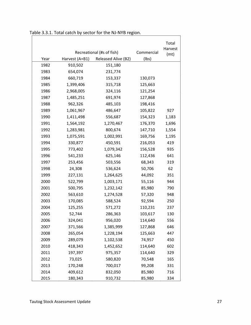
Tautog Stock Assessment Update 27
Table 3.3.1. Total catch by sector for the NJ‐NYB region.
Recreational (#s of fish) Commercial
Total Harvest (mt)
Year Harvest (A+B1) Released Alive (B2) (lbs)
1982 910,502 151,180
1983 654,074 231,774
1984 660,719 153,337 130,073
1985 1,399,406 315,718 125,663
1986 2,968,005 324,116 121,254
1987 1,485,251 691,974 127,868
1988 962,326 485,103 198,416
1989 1,061,967 486,647 105,822 927
1990 1,411,498 556,687 154,323 1,183
1991 1,564,192 1,270,467 176,370 1,696
1992 1,283,981 800,674 147,710 1,554
1993 1,075,591 1,002,991 169,756 1,195
1994 330,877 450,591 216,053 419
1995 773,402 1,079,342 156,528 935
1996 541,233 625,146 112,436 641
1997 253,456 503,556 68,343 319
1998 24,308 536,624 50,706 62
1999 227,131 1,264,625 44,092 351
2000 522,799 1,003,171 55,116 944
2001 500,795 1,232,142 85,980 790
2002 563,610 1,274,528 57,320 948
2003 170,085 588,524 92,594 250
2004 125,255 571,272 110,231 237
2005 52,744 286,363 103,617 130
2006 324,041 956,020 114,640 556
2007 371,566 1,385,999 127,868 646
2008 265,054 1,228,194 125,663 447
2009 289,079 1,102,538 74,957 450
2010 418,343 1,452,652 114,640 602
2011 197,397 975,357 114,640 329
2012 73,025 580,820 70,548 165
2013 170,248 700,017 99,208 331
2014 409,612 832,050 85,980 716
2015 180,343 910,732 85,980 334
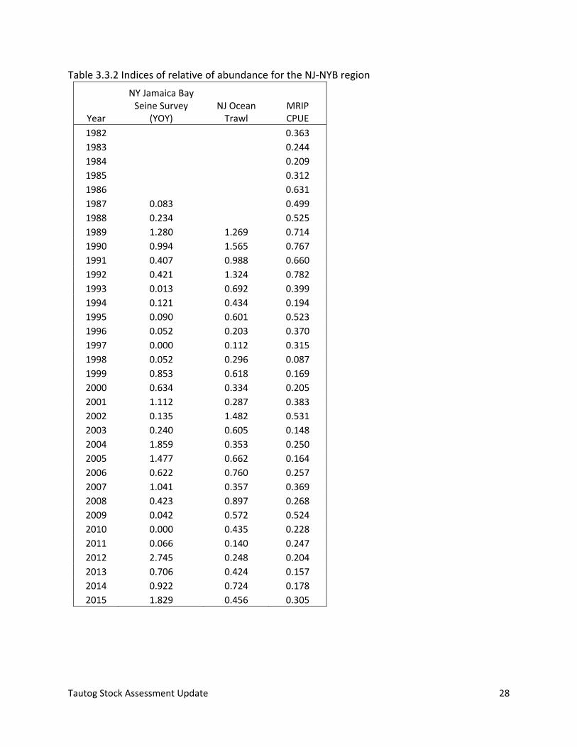
Tautog Stock Assessment Update 28
Table 3.3.2 Indices of relative of abundance for the NJ‐NYB region
Year
NY Jamaica Bay Seine Survey
(YOY)NJ Ocean Trawl
MRIP CPUE
1982 0.363
1983 0.244
1984 0.209
1985 0.312
1986 0.631
1987 0.083 0.499
1988 0.234 0.525
1989 1.280 1.269 0.714
1990 0.994 1.565 0.767
1991 0.407 0.988 0.660
1992 0.421 1.324 0.782
1993 0.013 0.692 0.399
1994 0.121 0.434 0.194
1995 0.090 0.601 0.523
1996 0.052 0.203 0.370
1997 0.000 0.112 0.315
1998 0.052 0.296 0.087
1999 0.853 0.618 0.169
2000 0.634 0.334 0.205
2001 1.112 0.287 0.383
2002 0.135 1.482 0.531
2003 0.240 0.605 0.148
2004 1.859 0.353 0.250
2005 1.477 0.662 0.164
2006 0.622 0.760 0.257
2007 1.041 0.357 0.369
2008 0.423 0.897 0.268
2009 0.042 0.572 0.524
2010 0.000 0.435 0.228
2011 0.066 0.140 0.247
2012 2.745 0.248 0.204
2013 0.706 0.424 0.157
2014 0.922 0.724 0.178
2015 1.829 0.456 0.305
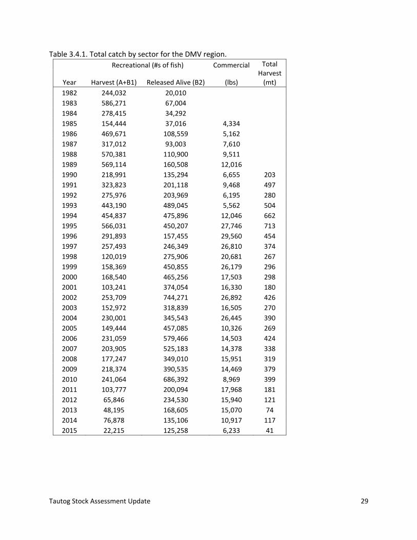
Tautog Stock Assessment Update 29
Table 3.4.1. Total catch by sector for the DMV region.
Recreational (#s of fish) Commercial Total Harvest (mt)Year Harvest (A+B1) Released Alive (B2) (lbs)
1982 244,032 20,010
1983 586,271 67,004
1984 278,415 34,292
1985 154,444 37,016 4,334
1986 469,671 108,559 5,162
1987 317,012 93,003 7,610
1988 570,381 110,900 9,511
1989 569,114 160,508 12,016
1990 218,991 135,294 6,655 203
1991 323,823 201,118 9,468 497
1992 275,976 203,969 6,195 280
1993 443,190 489,045 5,562 504
1994 454,837 475,896 12,046 662
1995 566,031 450,207 27,746 713
1996 291,893 157,455 29,560 454
1997 257,493 246,349 26,810 374
1998 120,019 275,906 20,681 267
1999 158,369 450,855 26,179 296
2000 168,540 465,256 17,503 298
2001 103,241 374,054 16,330 180
2002 253,709 744,271 26,892 426
2003 152,972 318,839 16,505 270
2004 230,001 345,543 26,445 390
2005 149,444 457,085 10,326 269
2006 231,059 579,466 14,503 424
2007 203,905 525,183 14,378 338
2008 177,247 349,010 15,951 319
2009 218,374 390,535 14,469 379
2010 241,064 686,392 8,969 399
2011 103,777 200,094 17,968 181
2012 65,846 234,530 15,940 121
2013 48,195 168,605 15,070 74
2014 76,878 135,106 10,917 117
2015 22,215 125,258 6,233 41
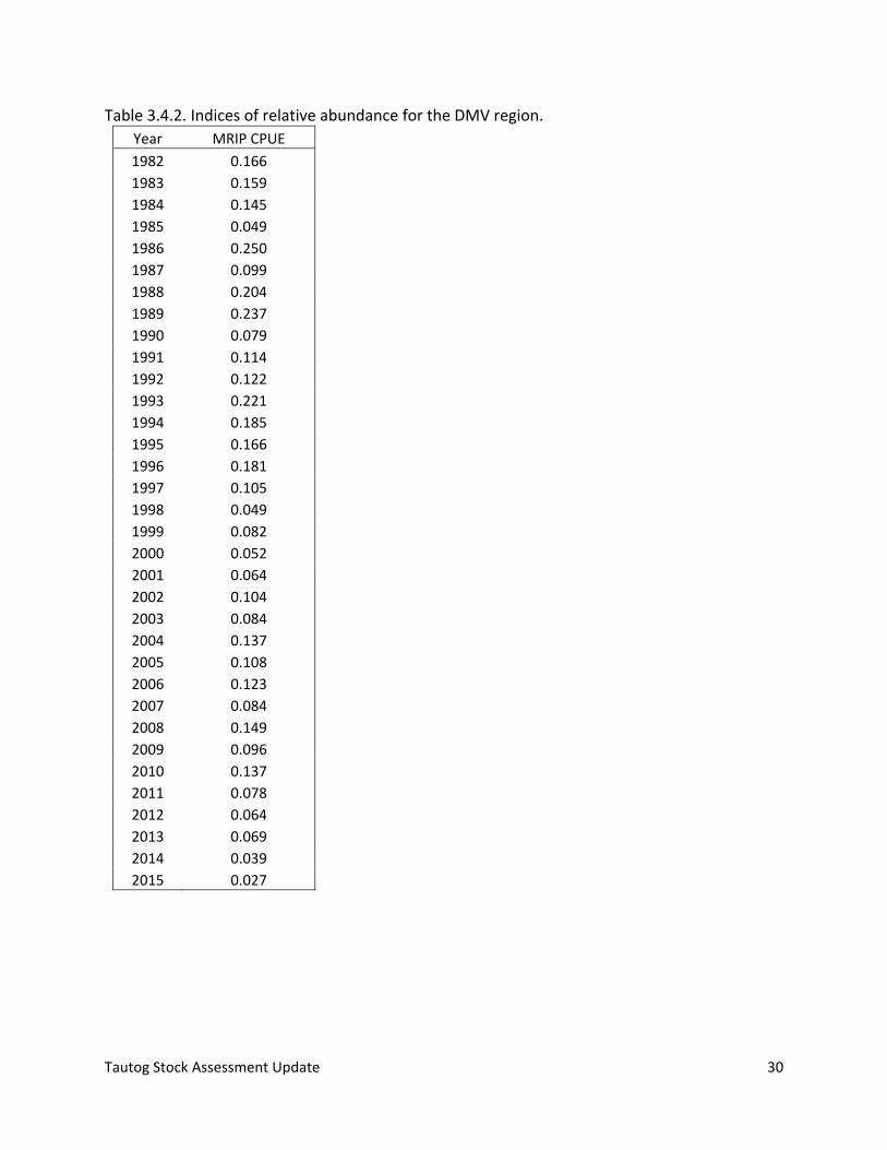
Tautog Stock Assessment Update 30
Table 3.4.2. Indices of relative abundance for the DMV region.
Year MRIP CPUE
1982 0.166
1983 0.159
1984 0.145
1985 0.049
1986 0.250
1987 0.099
1988 0.204
1989 0.237
1990 0.079
1991 0.114
1992 0.122
1993 0.221
1994 0.185
1995 0.166
1996 0.181
1997 0.105
1998 0.049
1999 0.082
2000 0.052
2001 0.064
2002 0.104
2003 0.084
2004 0.137
2005 0.108
2006 0.123
2007 0.084
2008 0.149
2009 0.096
2010 0.137
2011 0.078
2012 0.064
2013 0.069
2014 0.039
2015 0.027
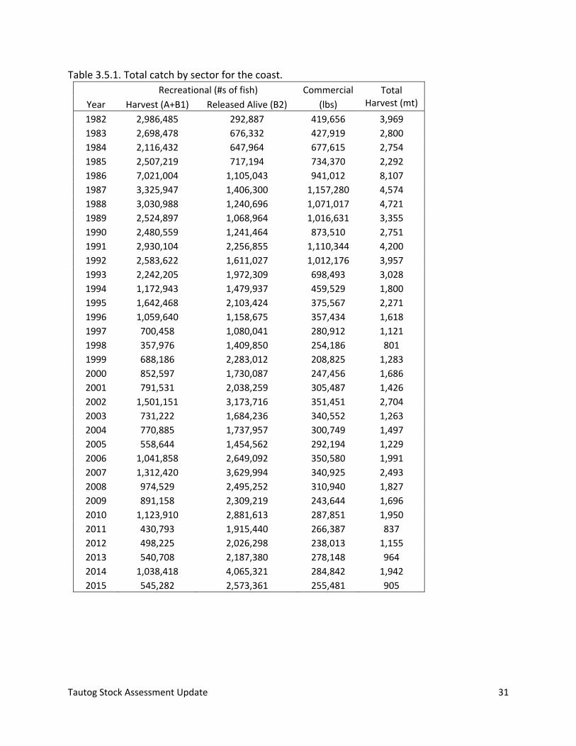
Tautog Stock Assessment Update 31
Table 3.5.1. Total catch by sector for the coast.
Recreational (#s of fish) Commercial Total Harvest (mt) Year Harvest (A+B1) Released Alive (B2) (lbs)
1982 2,986,485 292,887 419,656 3,969
1983 2,698,478 676,332 427,919 2,800
1984 2,116,432 647,964 677,615 2,754
1985 2,507,219 717,194 734,370 2,292
1986 7,021,004 1,105,043 941,012 8,107
1987 3,325,947 1,406,300 1,157,280 4,574
1988 3,030,988 1,240,696 1,071,017 4,721
1989 2,524,897 1,068,964 1,016,631 3,355
1990 2,480,559 1,241,464 873,510 2,751
1991 2,930,104 2,256,855 1,110,344 4,200
1992 2,583,622 1,611,027 1,012,176 3,957
1993 2,242,205 1,972,309 698,493 3,028
1994 1,172,943 1,479,937 459,529 1,800
1995 1,642,468 2,103,424 375,567 2,271
1996 1,059,640 1,158,675 357,434 1,618
1997 700,458 1,080,041 280,912 1,121
1998 357,976 1,409,850 254,186 801
1999 688,186 2,283,012 208,825 1,283
2000 852,597 1,730,087 247,456 1,686
2001 791,531 2,038,259 305,487 1,426
2002 1,501,151 3,173,716 351,451 2,704
2003 731,222 1,684,236 340,552 1,263
2004 770,885 1,737,957 300,749 1,497
2005 558,644 1,454,562 292,194 1,229
2006 1,041,858 2,649,092 350,580 1,991
2007 1,312,420 3,629,994 340,925 2,493
2008 974,529 2,495,252 310,940 1,827
2009 891,158 2,309,219 243,644 1,696
2010 1,123,910 2,881,613 287,851 1,950
2011 430,793 1,915,440 266,387 837
2012 498,225 2,026,298 238,013 1,155
2013 540,708 2,187,380 278,148 964
2014 1,038,418 4,065,321 284,842 1,942
2015 545,282 2,573,361 255,481 905
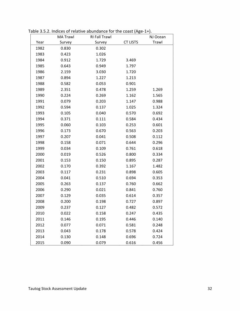
Tautog Stock Assessment Update 32
Table 3.5.2. Indices of relative abundance for the coast (Age‐1+).
Year MA Trawl Survey
RI Fall Trawl Survey CT LISTS
NJ Ocean Trawl
1982 0.830 0.302
1983 0.423 1.026
1984 0.912 1.729 3.469
1985 0.643 0.949 1.797
1986 2.159 3.030 1.720
1987 0.894 1.227 1.213
1988 0.582 0.053 0.901
1989 2.351 0.478 1.259 1.269
1990 0.224 0.269 1.162 1.565
1991 0.079 0.203 1.147 0.988
1992 0.594 0.137 1.025 1.324
1993 0.105 0.040 0.570 0.692
1994 0.371 0.111 0.584 0.434
1995 0.060 0.103 0.253 0.601
1996 0.173 0.670 0.563 0.203
1997 0.207 0.041 0.508 0.112
1998 0.158 0.071 0.644 0.296
1999 0.034 0.109 0.761 0.618
2000 0.019 0.526 0.800 0.334
2001 0.153 0.150 0.895 0.287
2002 0.170 0.392 1.167 1.482
2003 0.117 0.231 0.898 0.605
2004 0.041 0.510 0.694 0.353
2005 0.263 0.137 0.760 0.662
2006 0.290 0.021 0.841 0.760
2007 0.129 0.035 0.614 0.357
2008 0.200 0.198 0.727 0.897
2009 0.237 0.127 0.482 0.572
2010 0.022 0.158 0.247 0.435
2011 0.146 0.195 0.446 0.140
2012 0.077 0.071 0.581 0.248
2013 0.043 0.178 0.578 0.424
2014 0.130 0.148 0.696 0.724
2015 0.090 0.079 0.616 0.456
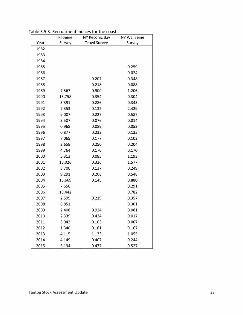
Tautog Stock Assessment Update 33
Table 3.5.3. Recruitment indices for the coast.
Year RI Seine Survey
NY Peconic Bay Trawl Survey
NY WLI Seine Survey
1982
1983
1984
1985 0.259
1986 0.024
1987 0.207 0.348
1988 0.218 0.088
1989 7.567 0.900 1.206
1990 13.758 0.354 0.304
1991 5.391 0.286 0.345
1992 7.353 0.132 2.429
1993 9.007 0.227 0.587
1994 3.507 0.076 0.014
1995 0.968 0.089 0.053
1996 0.877 0.233 0.135
1997 7.065 0.177 0.102
1998 2.658 0.250 0.204
1999 4.764 0.170 0.170
2000 5.313 0.085 1.193
2001 15.026 0.326 1.577
2002 8.700 0.137 0.249
2003 9.291 0.208 0.548
2004 15.669 0.145 0.880
2005 7.656 0.291
2006 13.442 0.782
2007 2.595 0.219 0.357
2008 8.851 0.301
2009 2.408 0.924 0.081
2010 2.339 0.424 0.017
2011 3.042 0.103 0.007
2012 1.340 0.161 0.167
2013 4.115 1.133 1.055
2014 4.149 0.407 0.244
2015 5.194 0.477 0.527
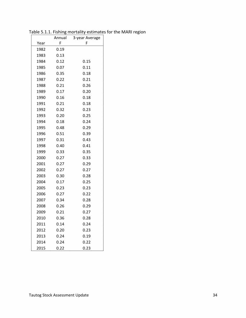
Tautog Stock Assessment Update 34
Table 5.1.1. Fishing mortality estimates for the MARI region
Year Annual
F 3‐year Average
F
1982 0.19
1983 0.13 1984 0.12 0.15 1985 0.07 0.11 1986 0.35 0.18 1987 0.22 0.21 1988 0.21 0.26 1989 0.17 0.20 1990 0.16 0.18 1991 0.21 0.18 1992 0.32 0.23
1993 0.20 0.25 1994 0.18 0.24 1995 0.48 0.29 1996 0.51 0.39 1997 0.31 0.43 1998 0.40 0.41 1999 0.33 0.35 2000 0.27 0.33 2001 0.27 0.29 2002 0.27 0.27 2003 0.30 0.28 2004 0.17 0.25 2005 0.23 0.23 2006 0.27 0.22 2007 0.34 0.28
2008 0.26 0.29 2009 0.21 0.27 2010 0.36 0.28 2011 0.14 0.24 2012 0.20 0.23 2013 0.24 0.19 2014 0.24 0.22 2015 0.22 0.23
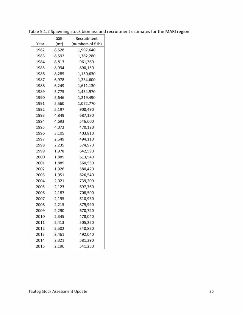
Tautog Stock Assessment Update 35
Table 5.1.2 Spawning stock biomass and recruitment estimates for the MARI region
Year SSB (mt)
Recruitment (numbers of fish)
1982 8,528 1,997,640 1983 8,592 1,382,280 1984 8,813 961,360 1985 8,994 890,150 1986 8,285 1,150,630 1987 6,978 1,234,600 1988 6,249 1,611,130 1989 5,775 1,454,970 1990 5,646 1,219,490 1991 5,560 1,072,770 1992 5,197 900,490
1993 4,849 687,180 1994 4,693 546,600 1995 4,072 470,120 1996 3,105 403,810 1997 2,549 494,110 1998 2,235 574,970 1999 1,978 642,590 2000 1,885 613,540 2001 1,889 560,550 2002 1,926 580,420 2003 1,951 626,540 2004 2,021 739,200 2005 2,123 697,760 2006 2,187 708,500 2007 2,195 610,950 2008 2,215 879,990 2009 2,290 670,720 2010 2,345 478,040 2011 2,413 505,250 2012 2,502 340,830 2013 2,461 492,040 2014 2,321 581,390
2015 2,196 541,250
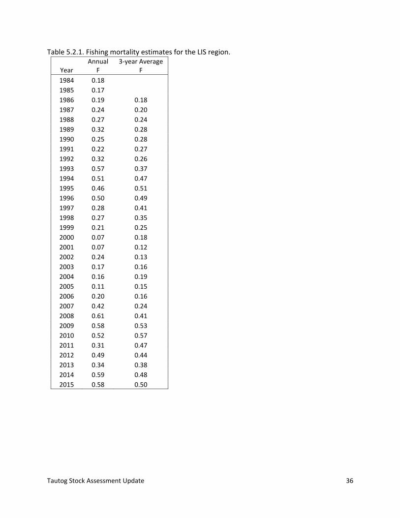
Tautog Stock Assessment Update 36
Table 5.2.1. Fishing mortality estimates for the LIS region.
Year Annual
F 3‐year Average
F
1984 0.18
1985 0.17 1986 0.19 0.18 1987 0.24 0.20 1988 0.27 0.24 1989 0.32 0.28 1990 0.25 0.28 1991 0.22 0.27 1992 0.32 0.26 1993 0.57 0.37 1994 0.51 0.47
1995 0.46 0.51 1996 0.50 0.49 1997 0.28 0.41 1998 0.27 0.35 1999 0.21 0.25 2000 0.07 0.18 2001 0.07 0.12 2002 0.24 0.13 2003 0.17 0.16 2004 0.16 0.19 2005 0.11 0.15 2006 0.20 0.16 2007 0.42 0.24 2008 0.61 0.41 2009 0.58 0.53
2010 0.52 0.57 2011 0.31 0.47 2012 0.49 0.44 2013 0.34 0.38 2014 0.59 0.48 2015 0.58 0.50
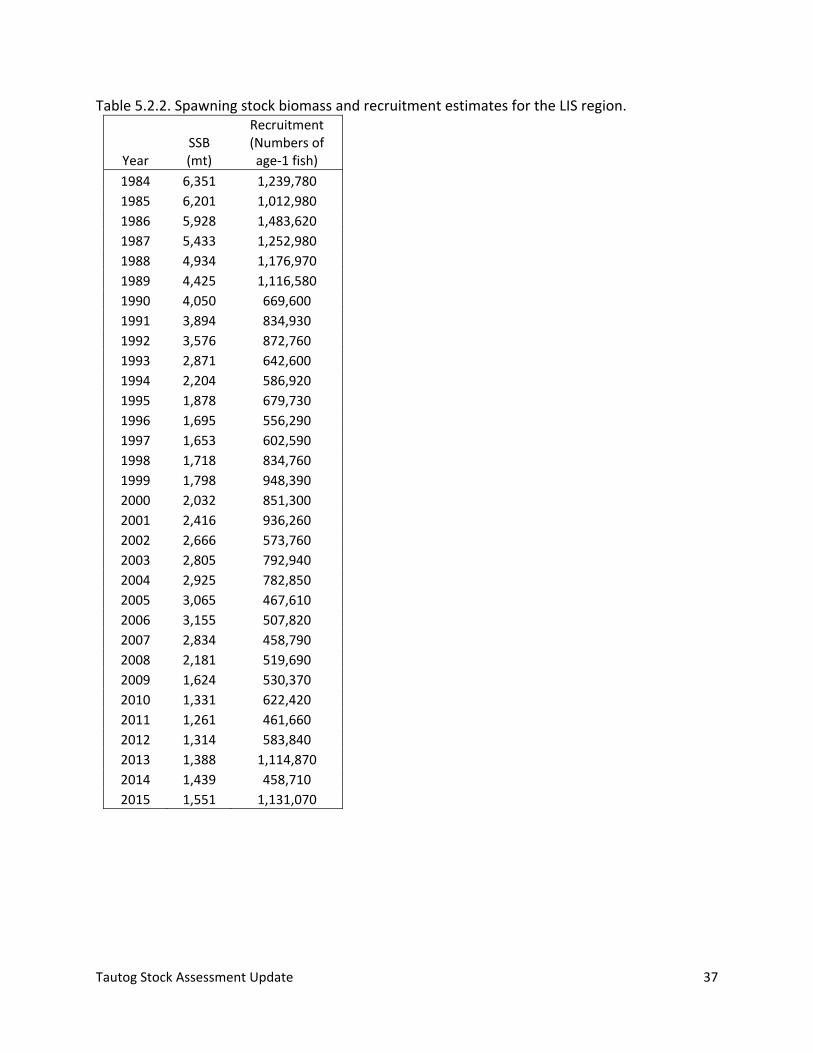
Tautog Stock Assessment Update 37
Table 5.2.2. Spawning stock biomass and recruitment estimates for the LIS region.
Year SSB (mt)
Recruitment (Numbers of age‐1 fish)
1984 6,351 1,239,780
1985 6,201 1,012,980 1986 5,928 1,483,620 1987 5,433 1,252,980 1988 4,934 1,176,970 1989 4,425 1,116,580 1990 4,050 669,600 1991 3,894 834,930 1992 3,576 872,760 1993 2,871 642,600
1994 2,204 586,920 1995 1,878 679,730 1996 1,695 556,290 1997 1,653 602,590 1998 1,718 834,760 1999 1,798 948,390 2000 2,032 851,300 2001 2,416 936,260 2002 2,666 573,760 2003 2,805 792,940 2004 2,925 782,850 2005 3,065 467,610 2006 3,155 507,820 2007 2,834 458,790 2008 2,181 519,690
2009 1,624 530,370 2010 1,331 622,420 2011 1,261 461,660 2012 1,314 583,840 2013 1,388 1,114,870 2014 1,439 458,710 2015 1,551 1,131,070

Tautog Stock Assessment Update 38
Table 5.3.1. Fishing mortality estimates for the NJ‐NYB region.
Year Annual
F 3‐Year Average
F
1989 0.23
1990 0.30 1991 0.49 0.34 1992 0.61 0.47 1993 0.65 0.59 1994 0.32 0.53 1995 0.58 0.52 1996 0.45 0.45 1997 0.25 0.43 1998 0.09 0.26 1999 0.19 0.18
2000 0.32 0.20 2001 0.41 0.31 2002 0.50 0.41 2003 0.23 0.38 2004 0.18 0.30 2005 0.11 0.17 2006 0.31 0.20 2007 0.45 0.29 2008 0.41 0.39 2009 0.45 0.43 2010 0.87 0.58 2011 0.58 0.63 2012 0.39 0.61 2013 0.52 0.50 2014 0.64 0.52
2015 0.45 0.54
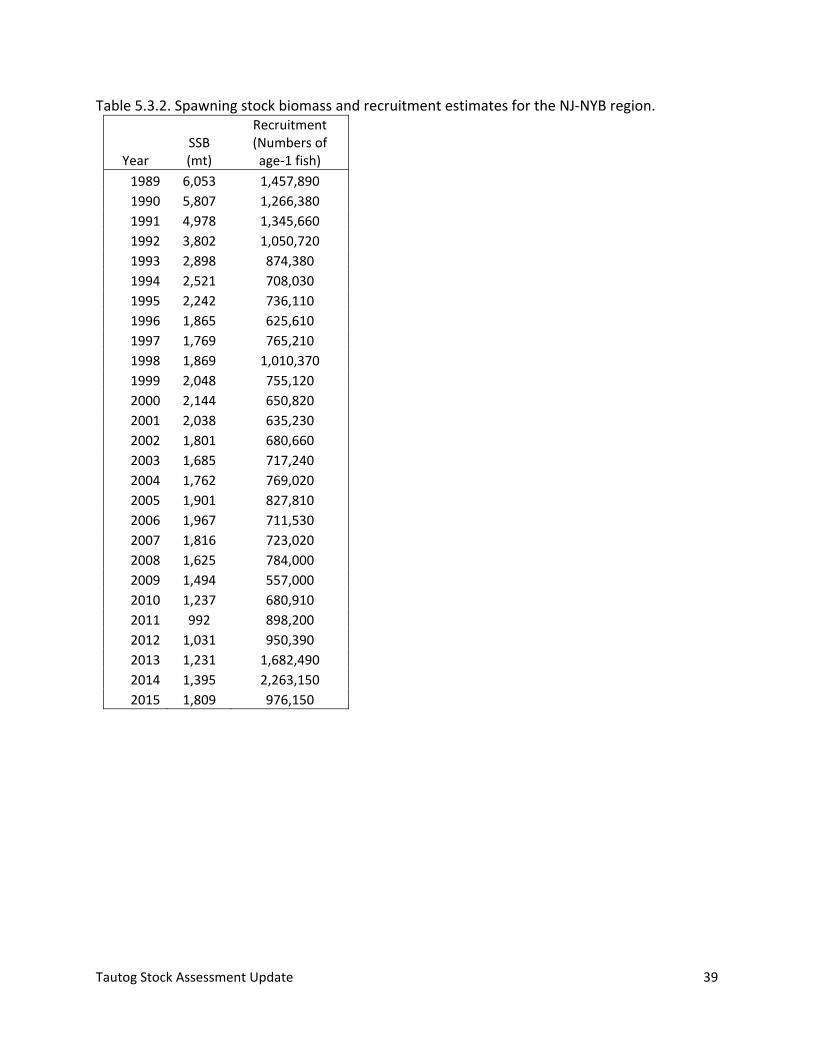
Tautog Stock Assessment Update 39
Table 5.3.2. Spawning stock biomass and recruitment estimates for the NJ‐NYB region.
Year SSB (mt)
Recruitment (Numbers of age‐1 fish)
1989 6,053 1,457,890
1990 5,807 1,266,380 1991 4,978 1,345,660 1992 3,802 1,050,720 1993 2,898 874,380 1994 2,521 708,030 1995 2,242 736,110 1996 1,865 625,610 1997 1,769 765,210 1998 1,869 1,010,370
1999 2,048 755,120 2000 2,144 650,820 2001 2,038 635,230 2002 1,801 680,660 2003 1,685 717,240 2004 1,762 769,020 2005 1,901 827,810 2006 1,967 711,530 2007 1,816 723,020 2008 1,625 784,000 2009 1,494 557,000 2010 1,237 680,910 2011 992 898,200 2012 1,031 950,390 2013 1,231 1,682,490
2014 1,395 2,263,150 2015 1,809 976,150
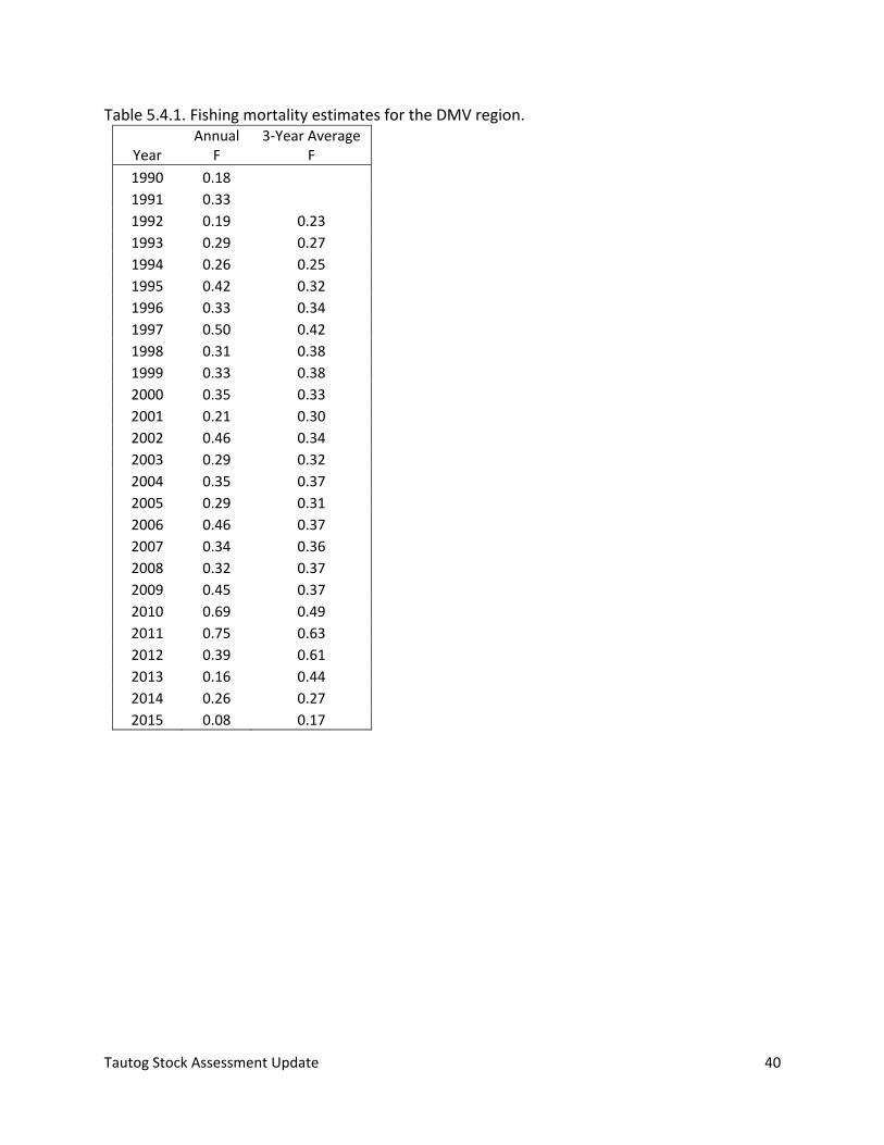
Tautog Stock Assessment Update 40
Table 5.4.1. Fishing mortality estimates for the DMV region.
Year Annual
F 3‐Year Average
F
1990 0.18
1991 0.33 1992 0.19 0.23 1993 0.29 0.27 1994 0.26 0.25 1995 0.42 0.32 1996 0.33 0.34 1997 0.50 0.42 1998 0.31 0.38 1999 0.33 0.38 2000 0.35 0.33
2001 0.21 0.30 2002 0.46 0.34 2003 0.29 0.32 2004 0.35 0.37 2005 0.29 0.31 2006 0.46 0.37 2007 0.34 0.36 2008 0.32 0.37 2009 0.45 0.37 2010 0.69 0.49 2011 0.75 0.63 2012 0.39 0.61 2013 0.16 0.44 2014 0.26 0.27 2015 0.08 0.17
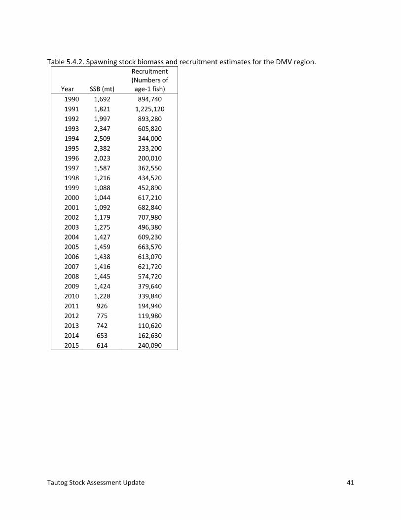
Tautog Stock Assessment Update 41
Table 5.4.2. Spawning stock biomass and recruitment estimates for the DMV region.
Year SSB (mt)
Recruitment (Numbers of age‐1 fish)
1990 1,692 894,740
1991 1,821 1,225,120
1992 1,997 893,280
1993 2,347 605,820
1994 2,509 344,000
1995 2,382 233,200
1996 2,023 200,010
1997 1,587 362,550
1998 1,216 434,520
1999 1,088 452,890
2000 1,044 617,210
2001 1,092 682,840
2002 1,179 707,980
2003 1,275 496,380
2004 1,427 609,230
2005 1,459 663,570
2006 1,438 613,070
2007 1,416 621,720
2008 1,445 574,720
2009 1,424 379,640
2010 1,228 339,840
2011 926 194,940
2012 775 119,980
2013 742 110,620
2014 653 162,630
2015 614 240,090
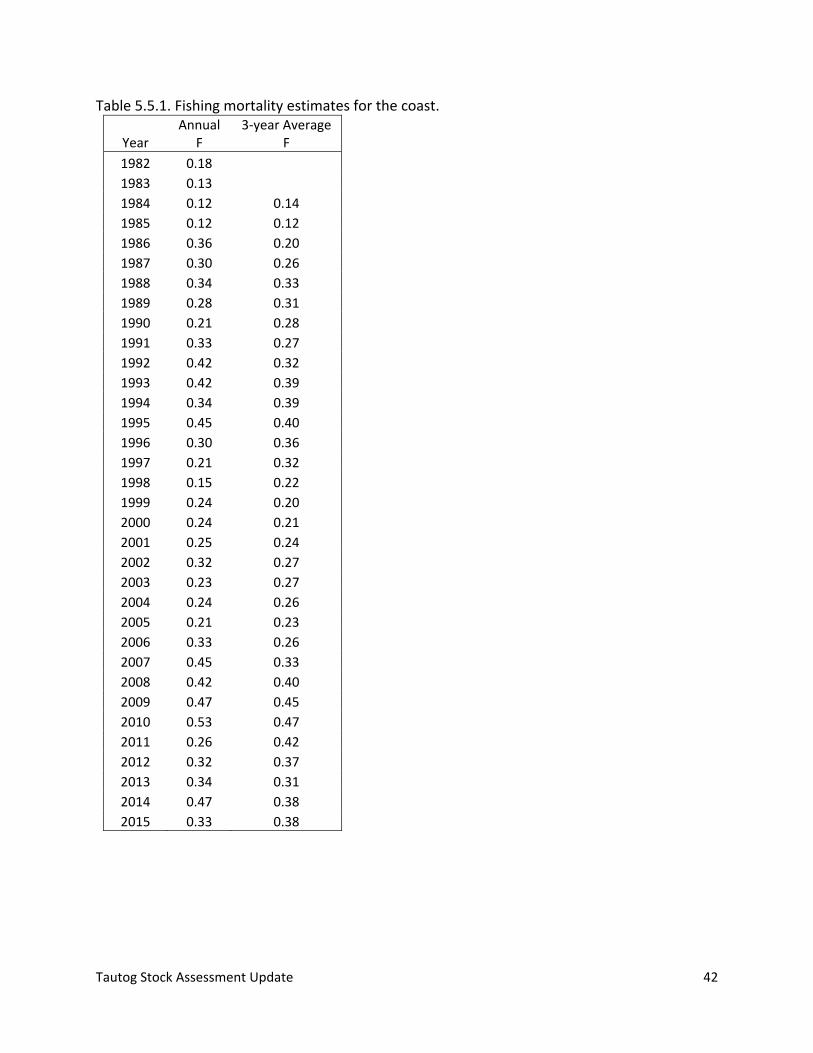
Tautog Stock Assessment Update 42
Table 5.5.1. Fishing mortality estimates for the coast.
Year Annual
F 3‐year Average
F
1982 0.18
1983 0.13 1984 0.12 0.14 1985 0.12 0.12 1986 0.36 0.20 1987 0.30 0.26 1988 0.34 0.33 1989 0.28 0.31 1990 0.21 0.28 1991 0.33 0.27 1992 0.42 0.32
1993 0.42 0.39 1994 0.34 0.39 1995 0.45 0.40 1996 0.30 0.36 1997 0.21 0.32 1998 0.15 0.22 1999 0.24 0.20 2000 0.24 0.21 2001 0.25 0.24 2002 0.32 0.27 2003 0.23 0.27 2004 0.24 0.26 2005 0.21 0.23 2006 0.33 0.26 2007 0.45 0.33
2008 0.42 0.40 2009 0.47 0.45 2010 0.53 0.47 2011 0.26 0.42 2012 0.32 0.37 2013 0.34 0.31 2014 0.47 0.38 2015 0.33 0.38
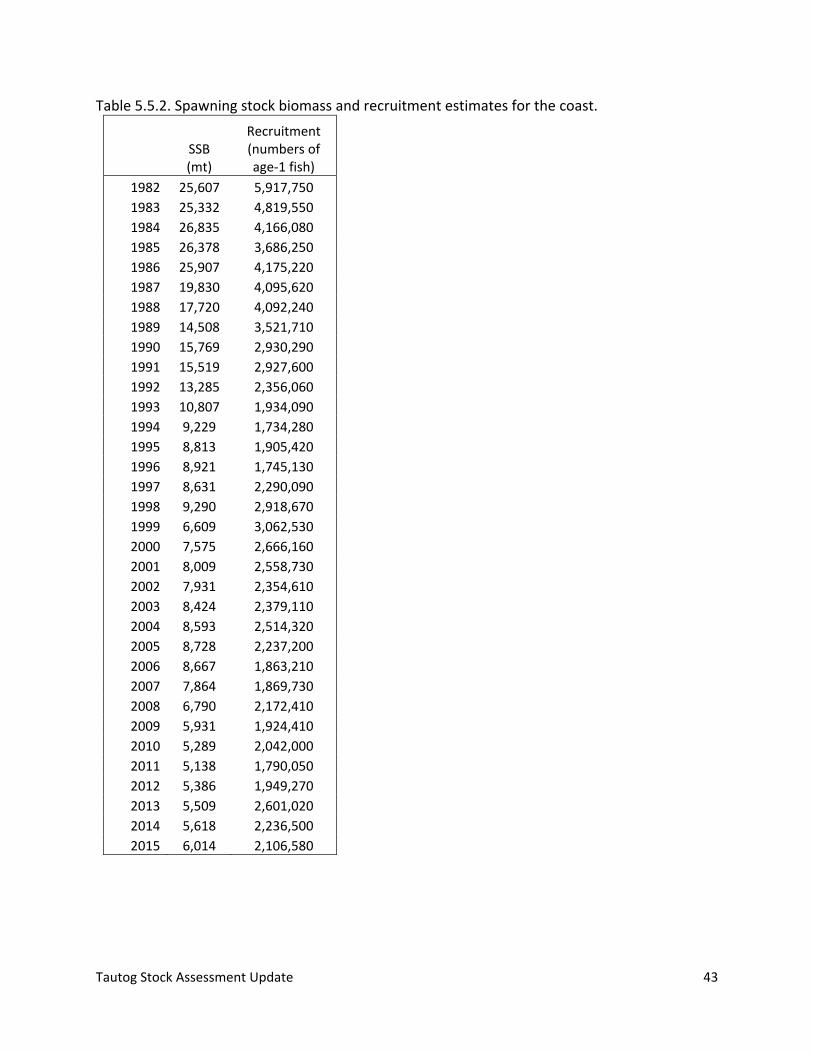
Tautog Stock Assessment Update 43
Table 5.5.2. Spawning stock biomass and recruitment estimates for the coast.
SSB (mt)
Recruitment (numbers of age‐1 fish)
1982 25,607 5,917,750 1983 25,332 4,819,550 1984 26,835 4,166,080 1985 26,378 3,686,250 1986 25,907 4,175,220 1987 19,830 4,095,620 1988 17,720 4,092,240 1989 14,508 3,521,710 1990 15,769 2,930,290 1991 15,519 2,927,600
1992 13,285 2,356,060 1993 10,807 1,934,090 1994 9,229 1,734,280 1995 8,813 1,905,420 1996 8,921 1,745,130 1997 8,631 2,290,090 1998 9,290 2,918,670 1999 6,609 3,062,530 2000 7,575 2,666,160 2001 8,009 2,558,730 2002 7,931 2,354,610 2003 8,424 2,379,110 2004 8,593 2,514,320 2005 8,728 2,237,200 2006 8,667 1,863,210 2007 7,864 1,869,730 2008 6,790 2,172,410 2009 5,931 1,924,410 2010 5,289 2,042,000 2011 5,138 1,790,050 2012 5,386 1,949,270 2013 5,509 2,601,020
2014 5,618 2,236,500 2015 6,014 2,106,580
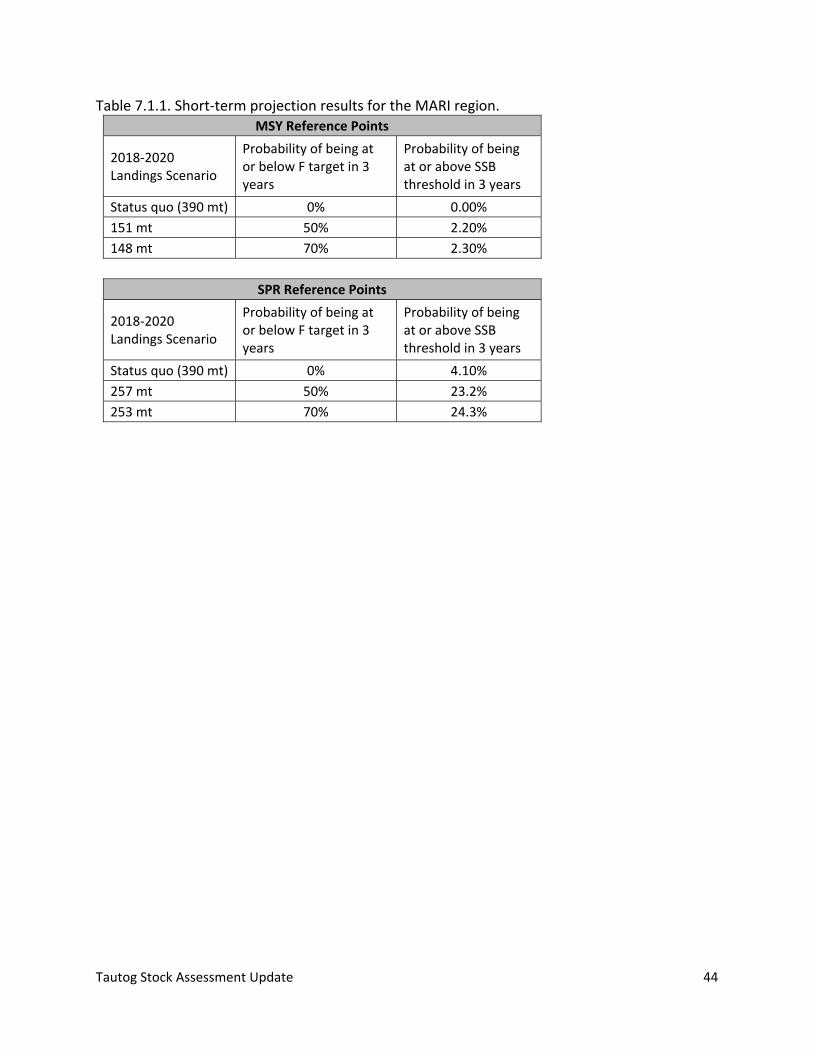
Tautog Stock Assessment Update 44
Table 7.1.1. Short‐term projection results for the MARI region. MSY Reference Points
2018‐2020 Landings Scenario
Probability of being at or below F target in 3 years
Probability of being at or above SSB threshold in 3 years
Status quo (390 mt) 0% 0.00%
151 mt 50% 2.20%
148 mt 70% 2.30%
SPR Reference Points
2018‐2020 Landings Scenario
Probability of being at or below F target in 3 years
Probability of being at or above SSB threshold in 3 years
Status quo (390 mt) 0% 4.10%
257 mt 50% 23.2%
253 mt 70% 24.3%
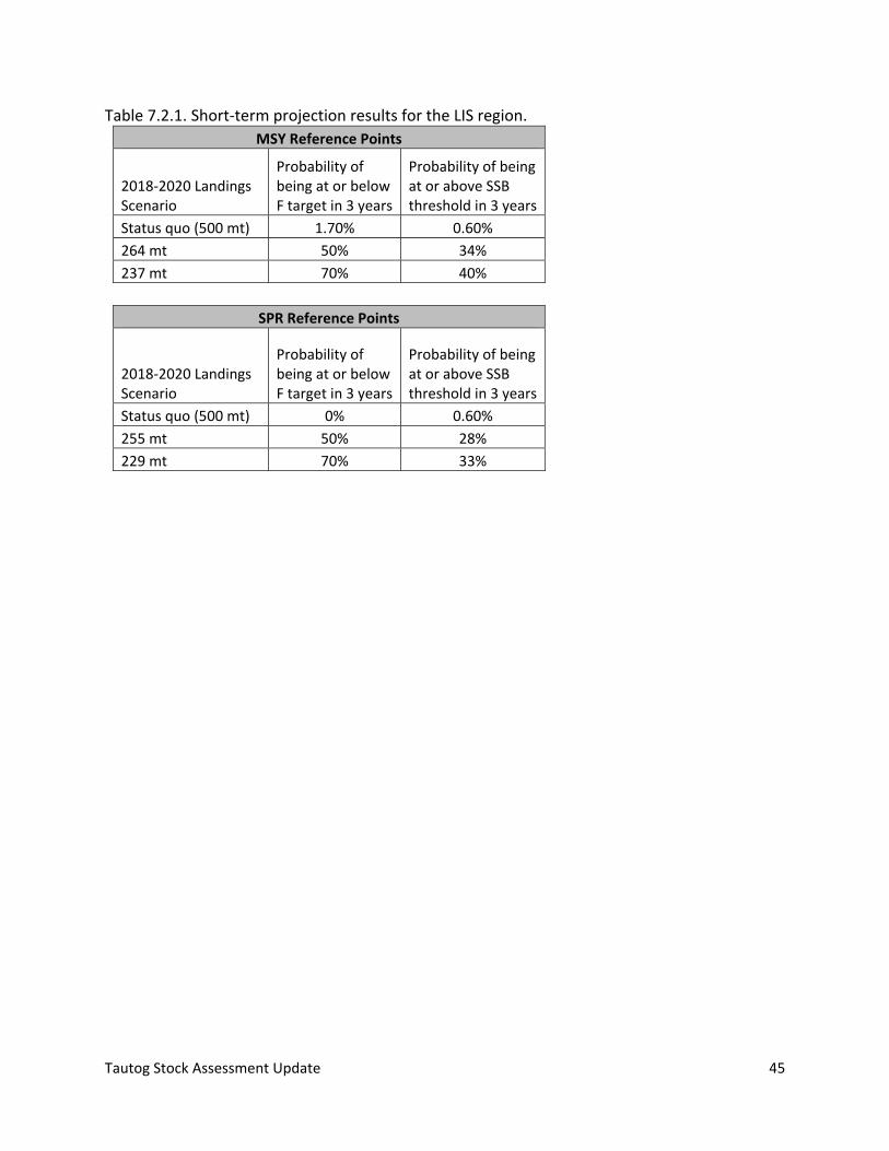
Tautog Stock Assessment Update 45
Table 7.2.1. Short‐term projection results for the LIS region.
MSY Reference Points
2018‐2020 Landings Scenario
Probability of being at or below F target in 3 years
Probability of being at or above SSB threshold in 3 years
Status quo (500 mt) 1.70% 0.60%
264 mt 50% 34%
237 mt 70% 40%
SPR Reference Points
2018‐2020 Landings Scenario
Probability of being at or below F target in 3 years
Probability of being at or above SSB threshold in 3 years
Status quo (500 mt) 0% 0.60%
255 mt 50% 28%
229 mt 70% 33%
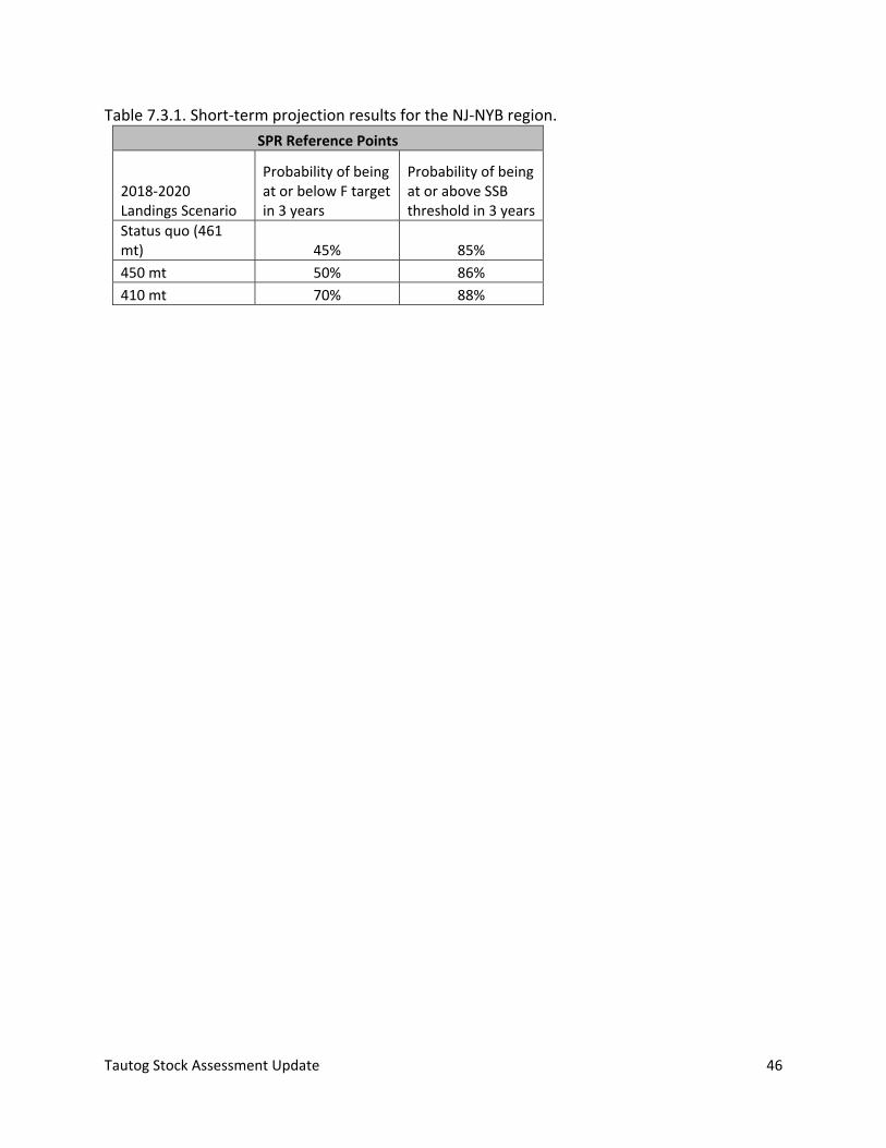
Tautog Stock Assessment Update 46
Table 7.3.1. Short‐term projection results for the NJ‐NYB region.
SPR Reference Points
2018‐2020 Landings Scenario
Probability of being at or below F target in 3 years
Probability of being at or above SSB threshold in 3 years
Status quo (461 mt) 45% 85%
450 mt 50% 86%
410 mt 70% 88%
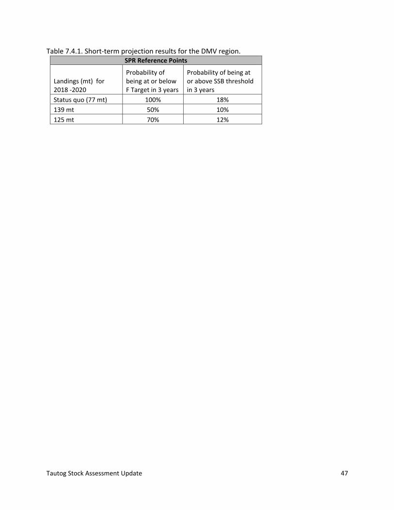
Tautog Stock Assessment Update 47
Table 7.4.1. Short‐term projection results for the DMV region. SPR Reference Points
Landings (mt) for 2018 ‐2020
Probability of being at or below F Target in 3 years
Probability of being at or above SSB threshold in 3 years
Status quo (77 mt) 100% 18%
139 mt 50% 10%
125 mt 70% 12%
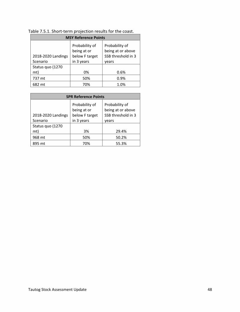
Tautog Stock Assessment Update 48
Table 7.5.1. Short‐term projection results for the coast.
MSY Reference Points
2018‐2020 Landings Scenario
Probability of being at or below F target in 3 years
Probability of being at or above SSB threshold in 3 years
Status quo (1270 mt) 0% 0.6%
737 mt 50% 0.9%
682 mt 70% 1.0%
SPR Reference Points
2018‐2020 Landings Scenario
Probability of being at or below F target in 3 years
Probability of being at or above SSB threshold in 3 years
Status quo (1270 mt) 3% 29.4%
968 mt 50% 50.2%
895 mt 70% 55.3%

Tautog Stock Assessment Update 49
11 Figures
Figure 3.1.1. Total removals by sector for the MARI region.
MARI
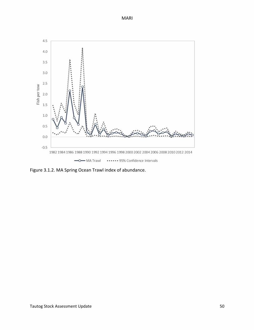
MARI
Tautog Stock Assessment Update 50
Figure 3.1.2. MA Spring Ocean Trawl index of abundance.
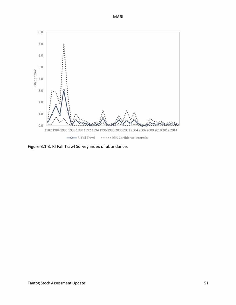
MARI
Tautog Stock Assessment Update 51
Figure 3.1.3. RI Fall Trawl Survey index of abundance.
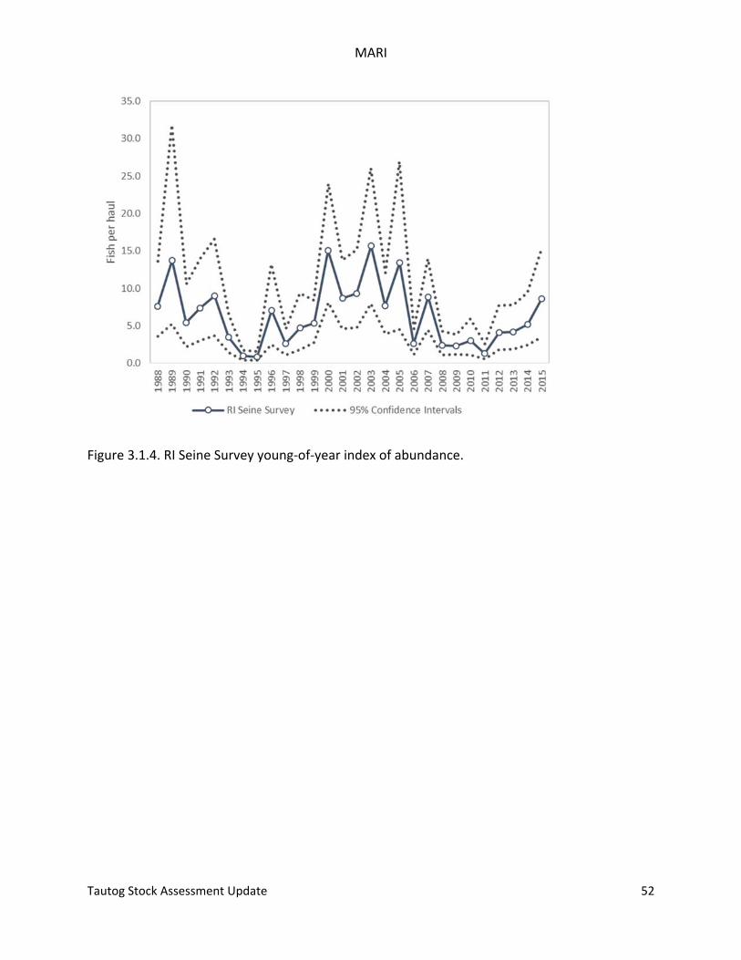
MARI
Tautog Stock Assessment Update 52
Figure 3.1.4. RI Seine Survey young‐of‐year index of abundance.
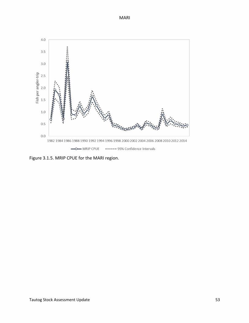
MARI
Tautog Stock Assessment Update 53
Figure 3.1.5. MRIP CPUE for the MARI region.
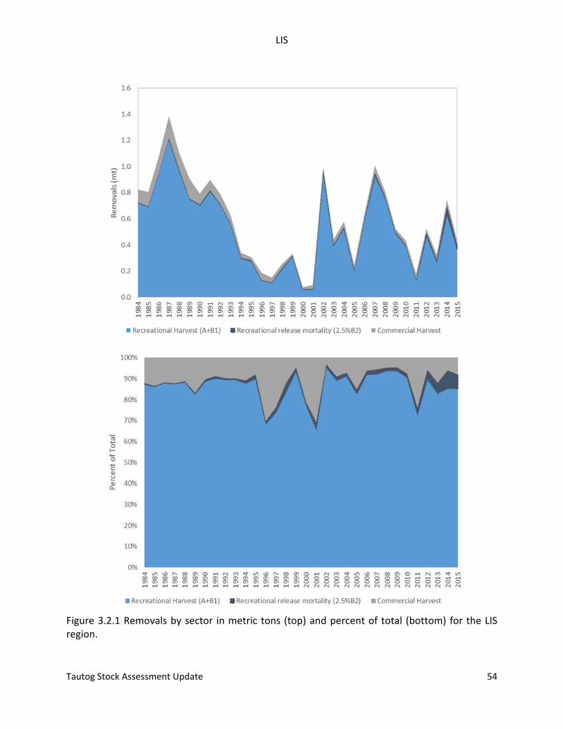
LIS
Tautog Stock Assessment Update 54
Figure 3.2.1 Removals by sector in metric tons (top) and percent of total (bottom) for the LIS region.
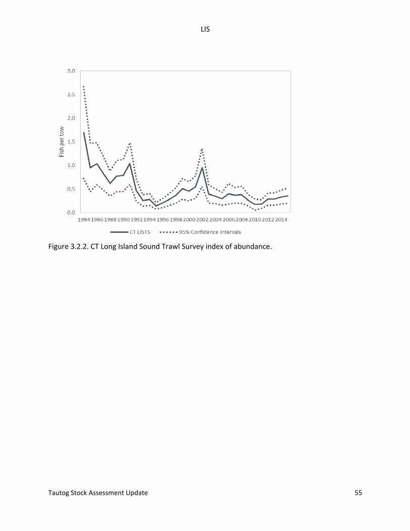
LIS
Tautog Stock Assessment Update 55
Figure 3.2.2. CT Long Island Sound Trawl Survey index of abundance.
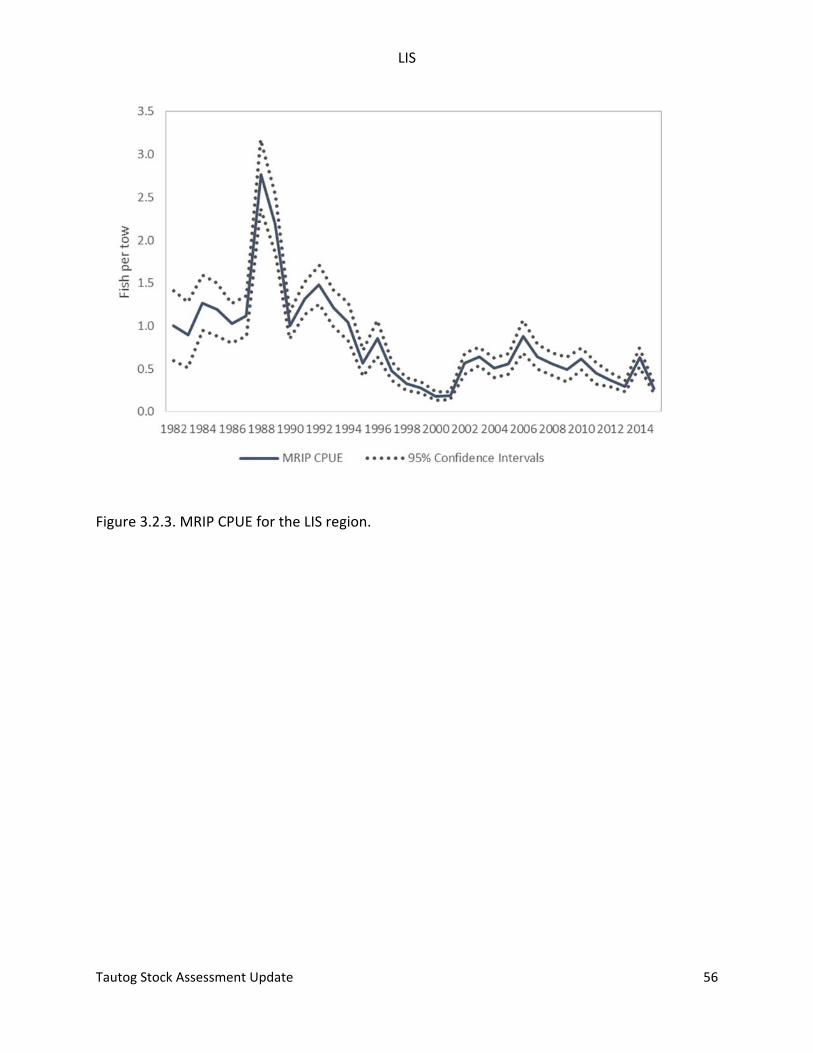
LIS
Tautog Stock Assessment Update 56
Figure 3.2.3. MRIP CPUE for the LIS region.
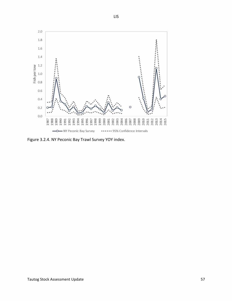
LIS
Tautog Stock Assessment Update 57
Figure 3.2.4. NY Peconic Bay Trawl Survey YOY index.
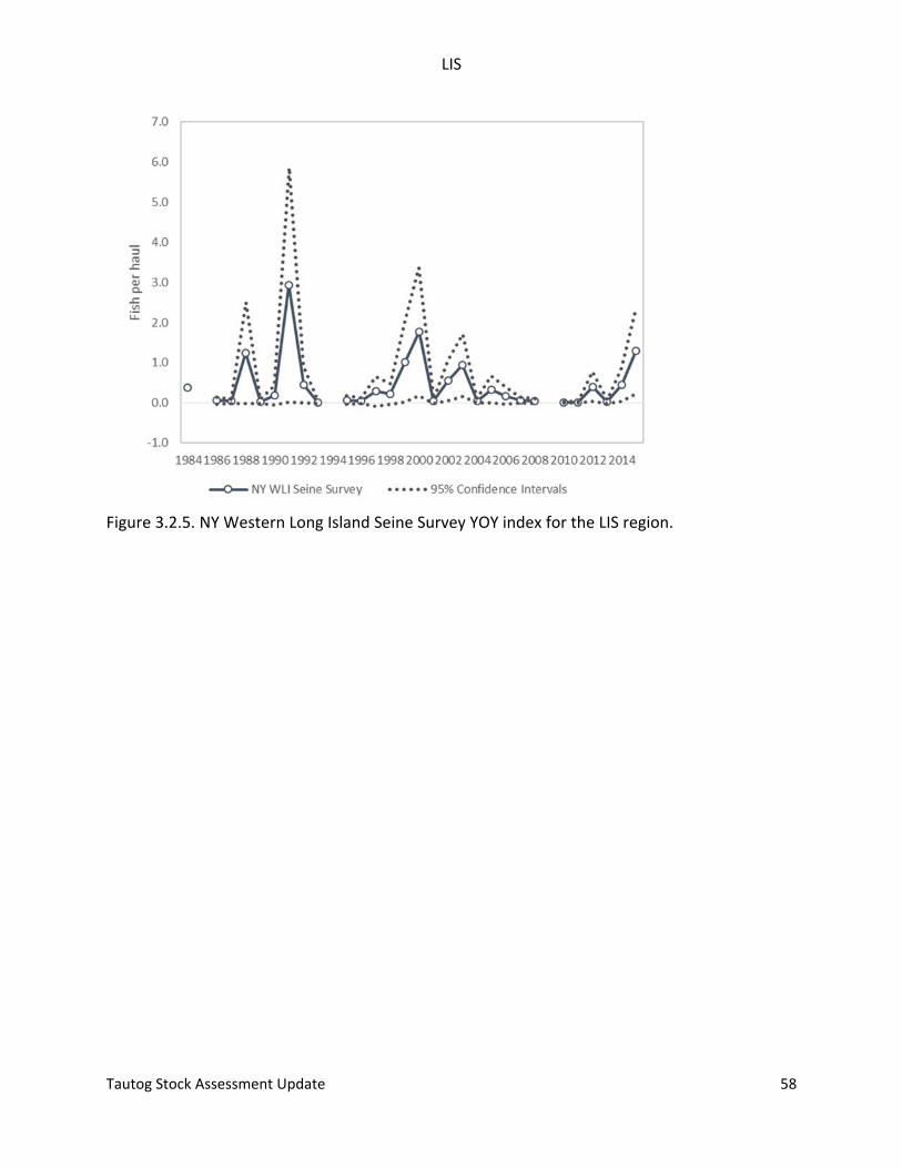
LIS
Tautog Stock Assessment Update 58
Figure 3.2.5. NY Western Long Island Seine Survey YOY index for the LIS region.
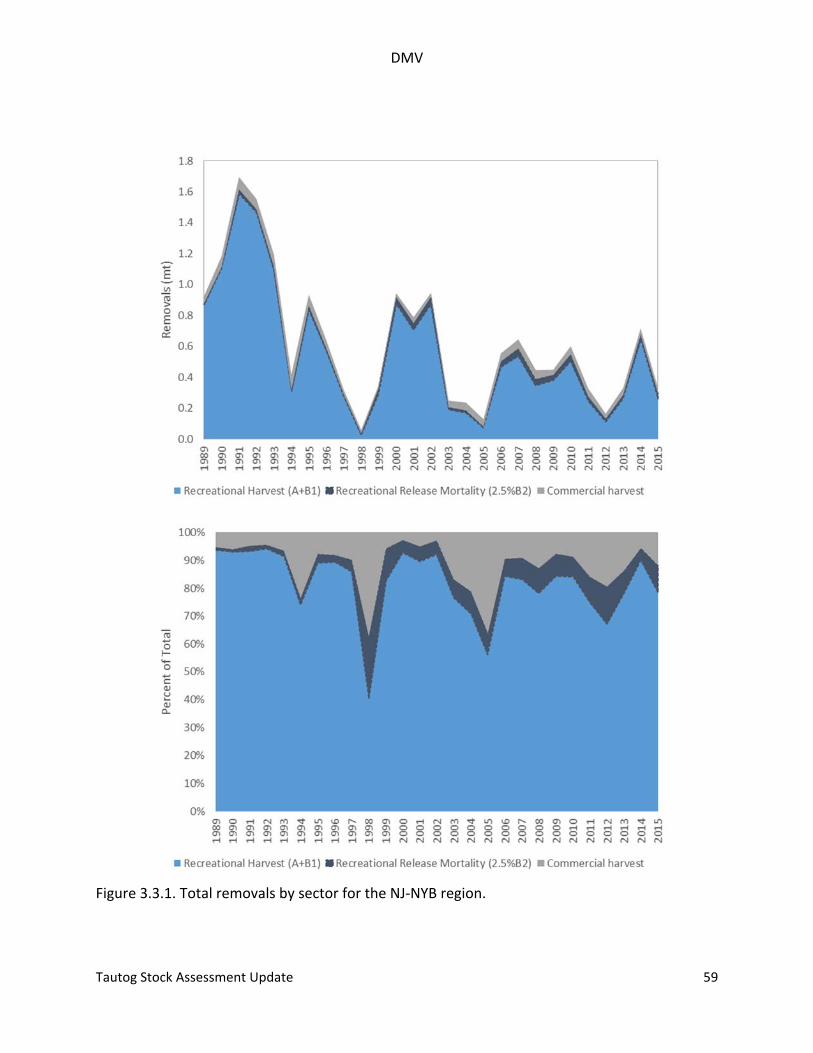
DMV
Tautog Stock Assessment Update 59
Figure 3.3.1. Total removals by sector for the NJ‐NYB region.
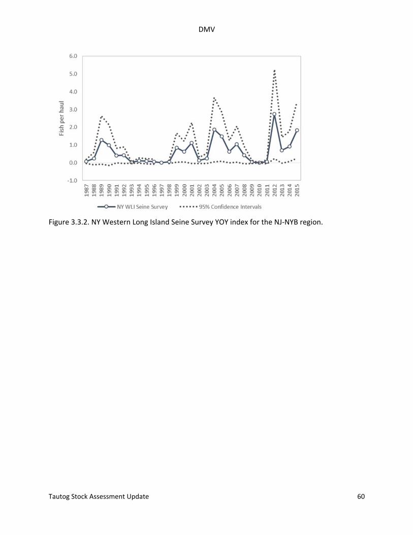
DMV
Tautog Stock Assessment Update 60
Figure 3.3.2. NY Western Long Island Seine Survey YOY index for the NJ‐NYB region.
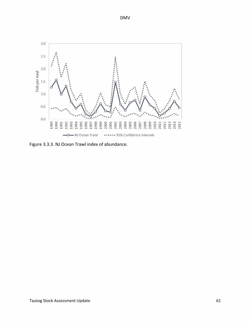
DMV
Tautog Stock Assessment Update 61
Figure 3.3.3. NJ Ocean Trawl index of abundance.
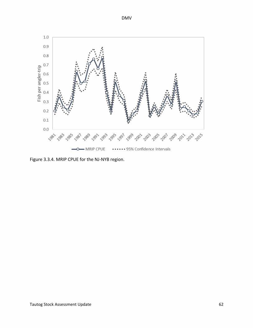
DMV
Tautog Stock Assessment Update 62
Figure 3.3.4. MRIP CPUE for the NJ‐NYB region.
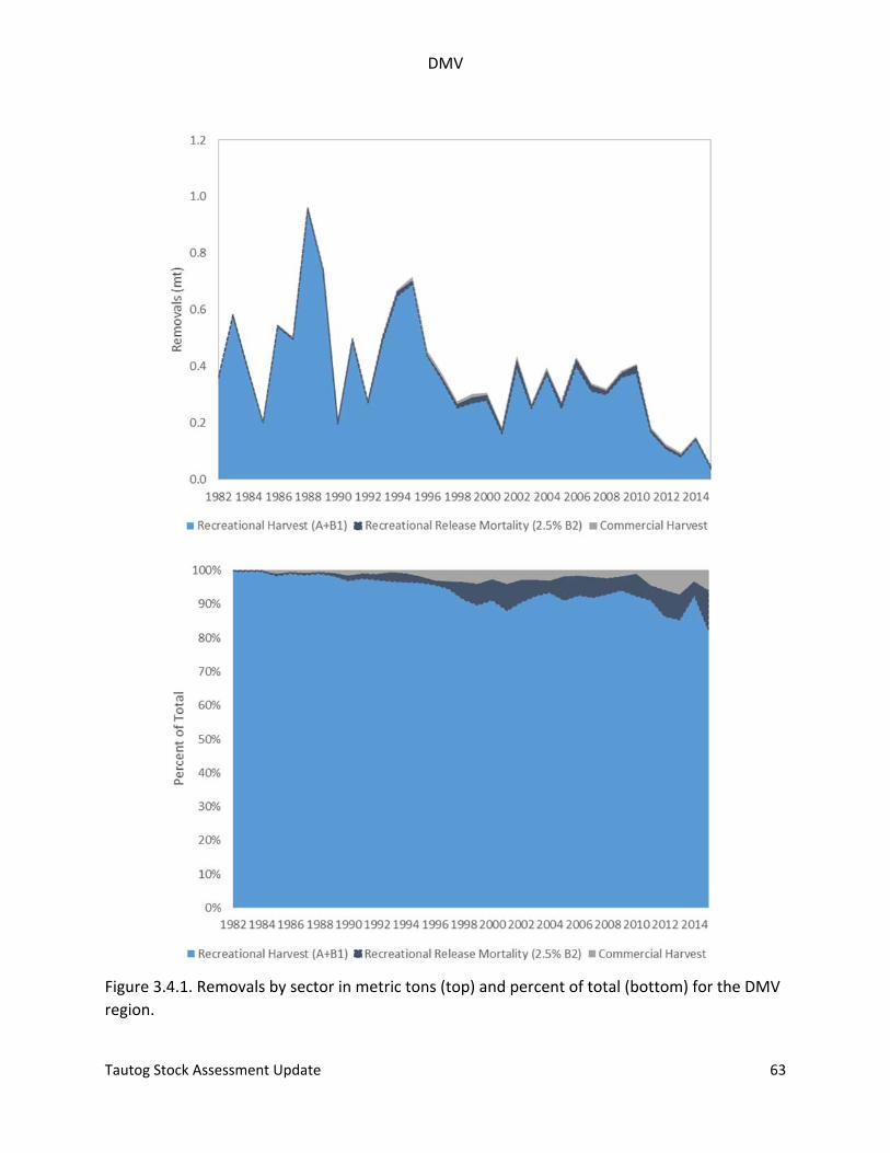
DMV
Tautog Stock Assessment Update 63
Figure 3.4.1. Removals by sector in metric tons (top) and percent of total (bottom) for the DMV
region.
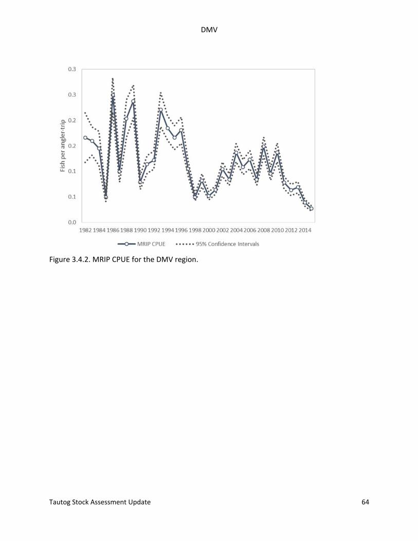
DMV
Tautog Stock Assessment Update 64
Figure 3.4.2. MRIP CPUE for the DMV region.
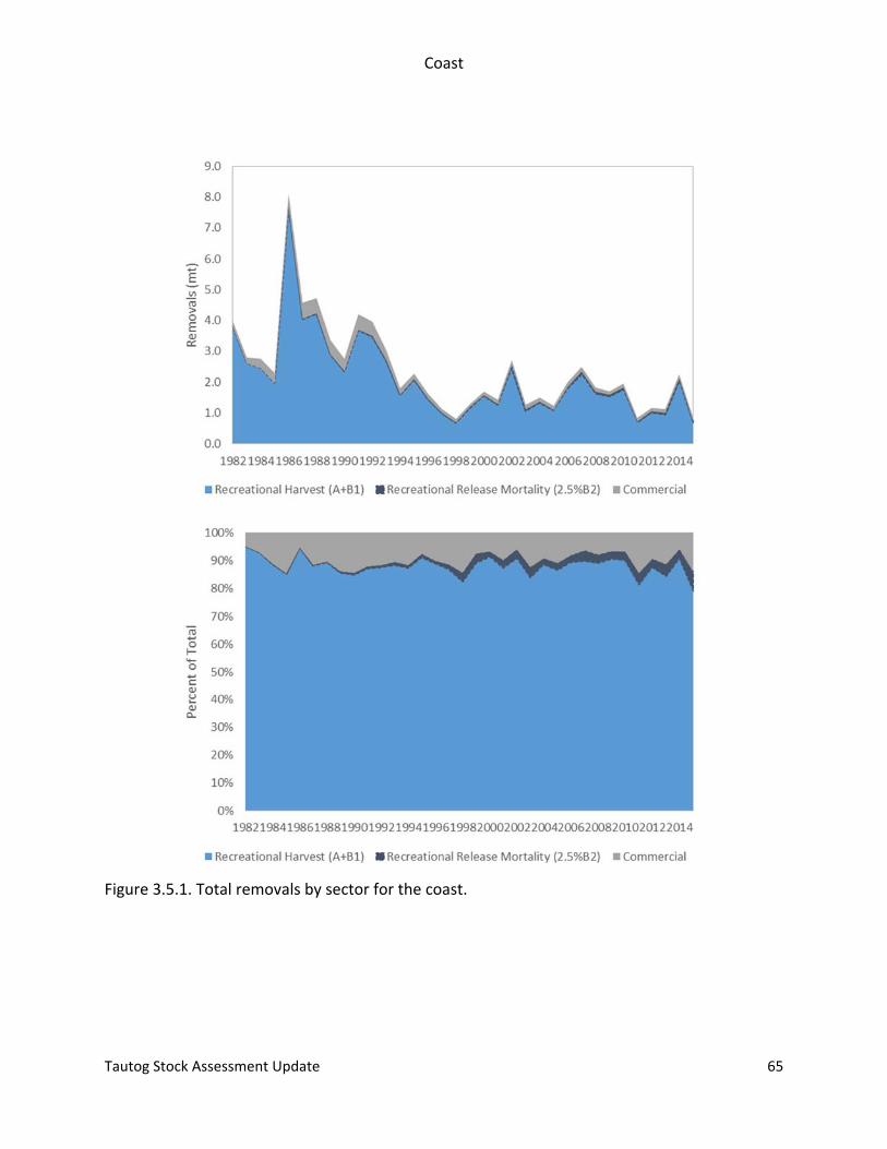
Coast
Tautog Stock Assessment Update 65
Figure 3.5.1. Total removals by sector for the coast.
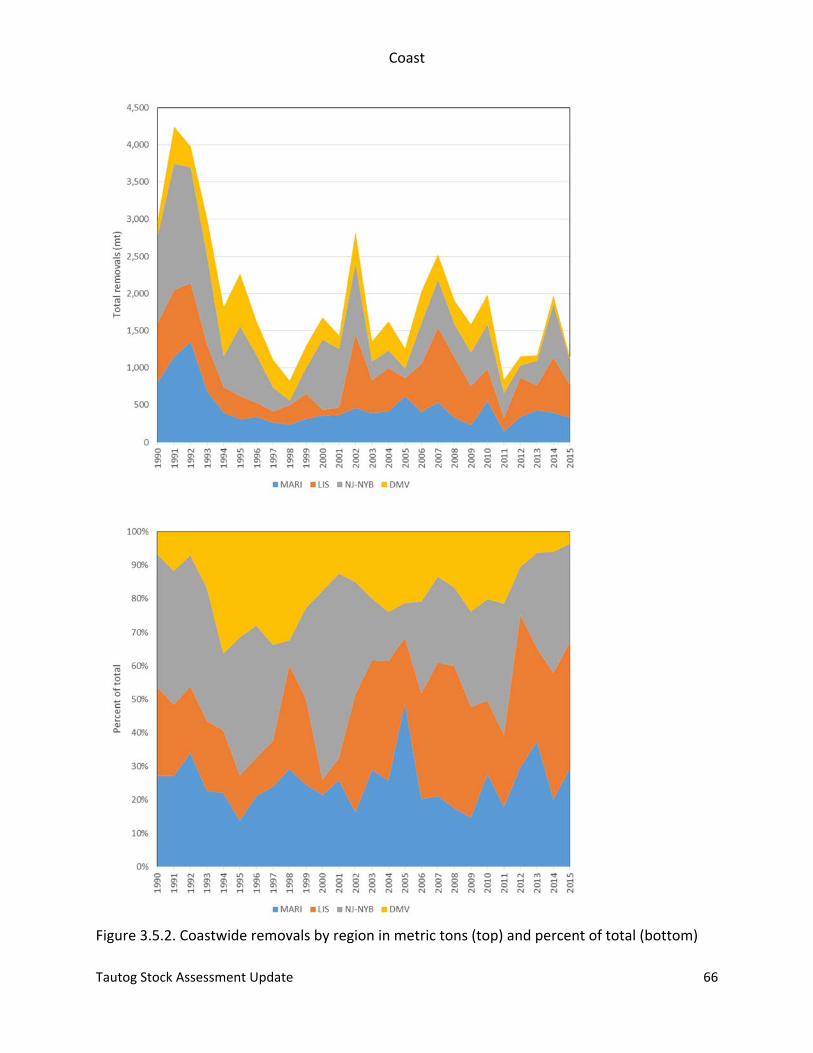
Coast
Tautog Stock Assessment Update 66
Figure 3.5.2. Coastwide removals by region in metric tons (top) and percent of total (bottom)
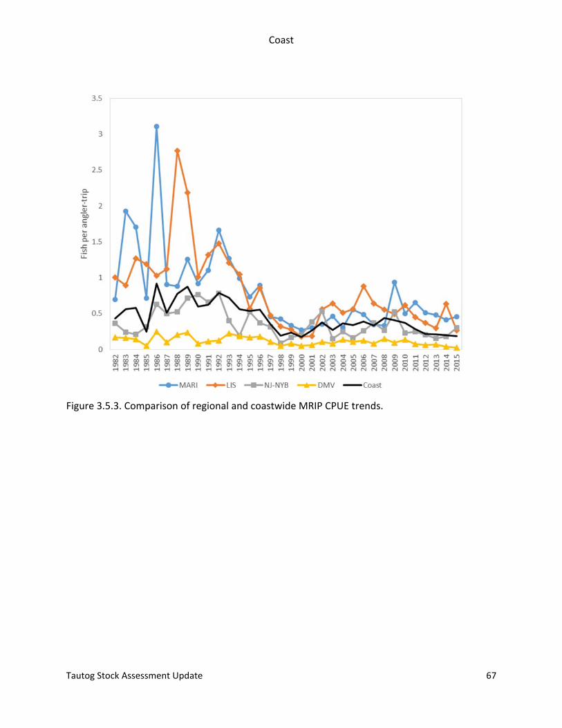
Coast
Tautog Stock Assessment Update 67
Figure 3.5.3. Comparison of regional and coastwide MRIP CPUE trends.
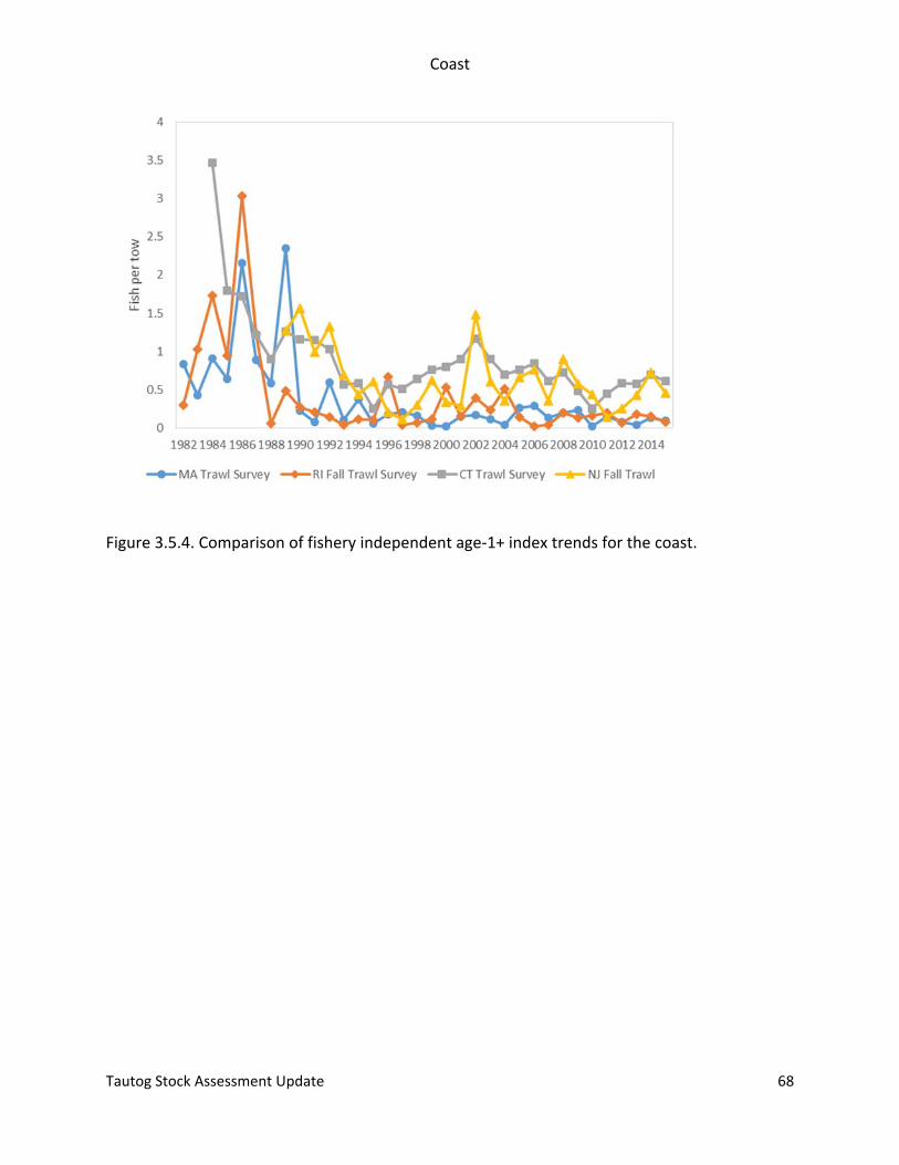
Coast
Tautog Stock Assessment Update 68
Figure 3.5.4. Comparison of fishery independent age‐1+ index trends for the coast.
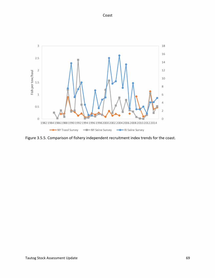
Coast
Tautog Stock Assessment Update 69
Figure 3.5.5. Comparison of fishery independent recruitment index trends for the coast.
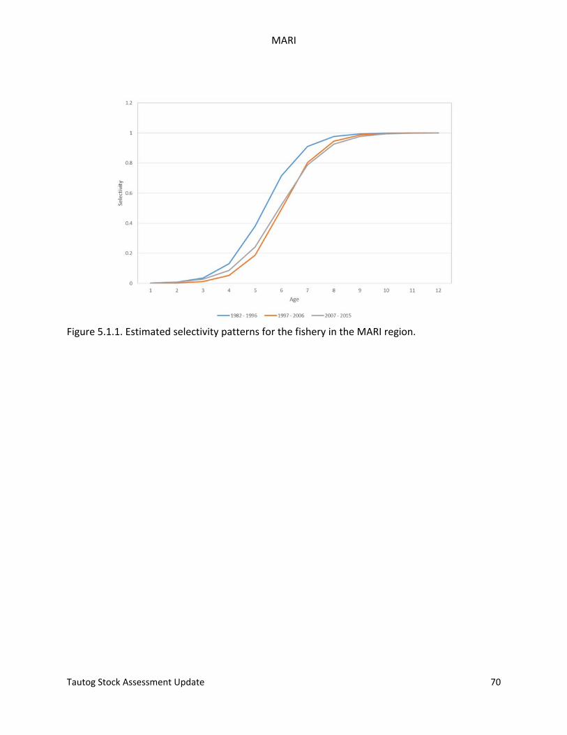
MARI
Tautog Stock Assessment Update 70
Figure 5.1.1. Estimated selectivity patterns for the fishery in the MARI region.
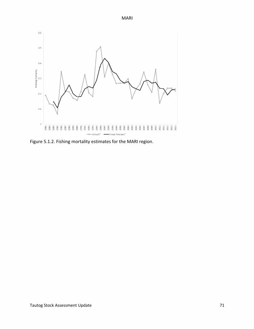
MARI
Tautog Stock Assessment Update 71
Figure 5.1.2. Fishing mortality estimates for the MARI region.
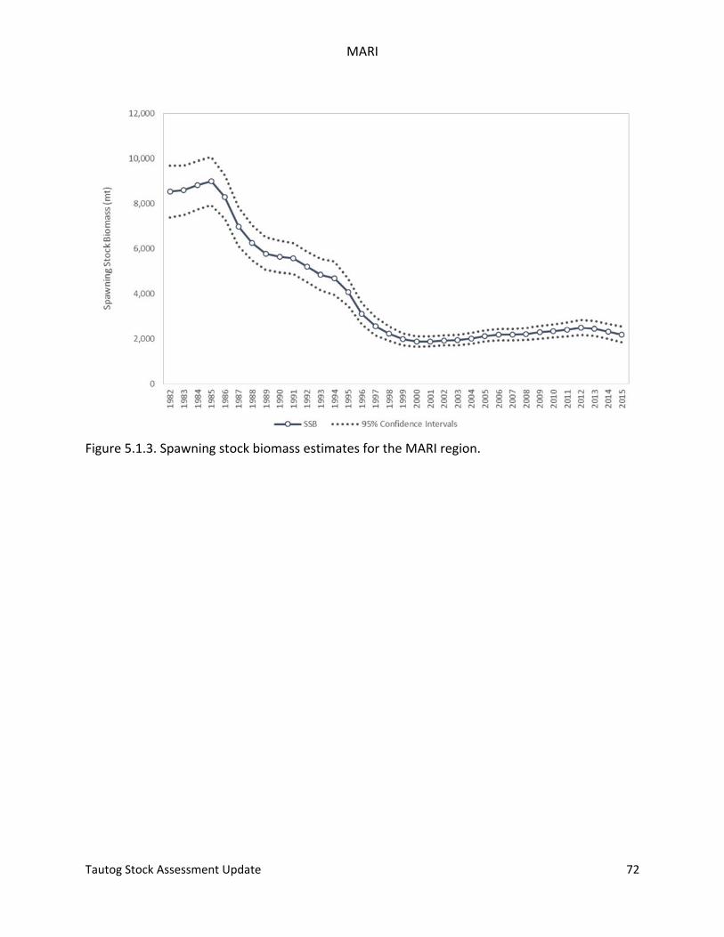
MARI
Tautog Stock Assessment Update 72
Figure 5.1.3. Spawning stock biomass estimates for the MARI region.
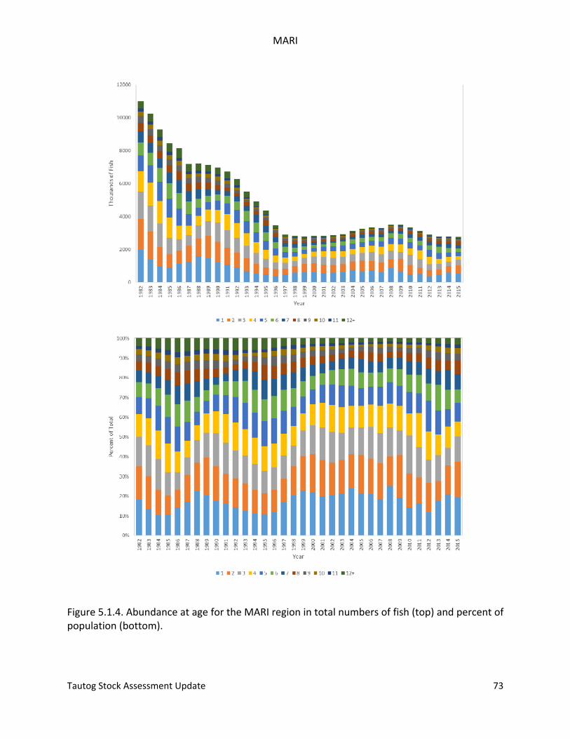
MARI
Tautog Stock Assessment Update 73
Figure 5.1.4. Abundance at age for the MARI region in total numbers of fish (top) and percent of population (bottom).
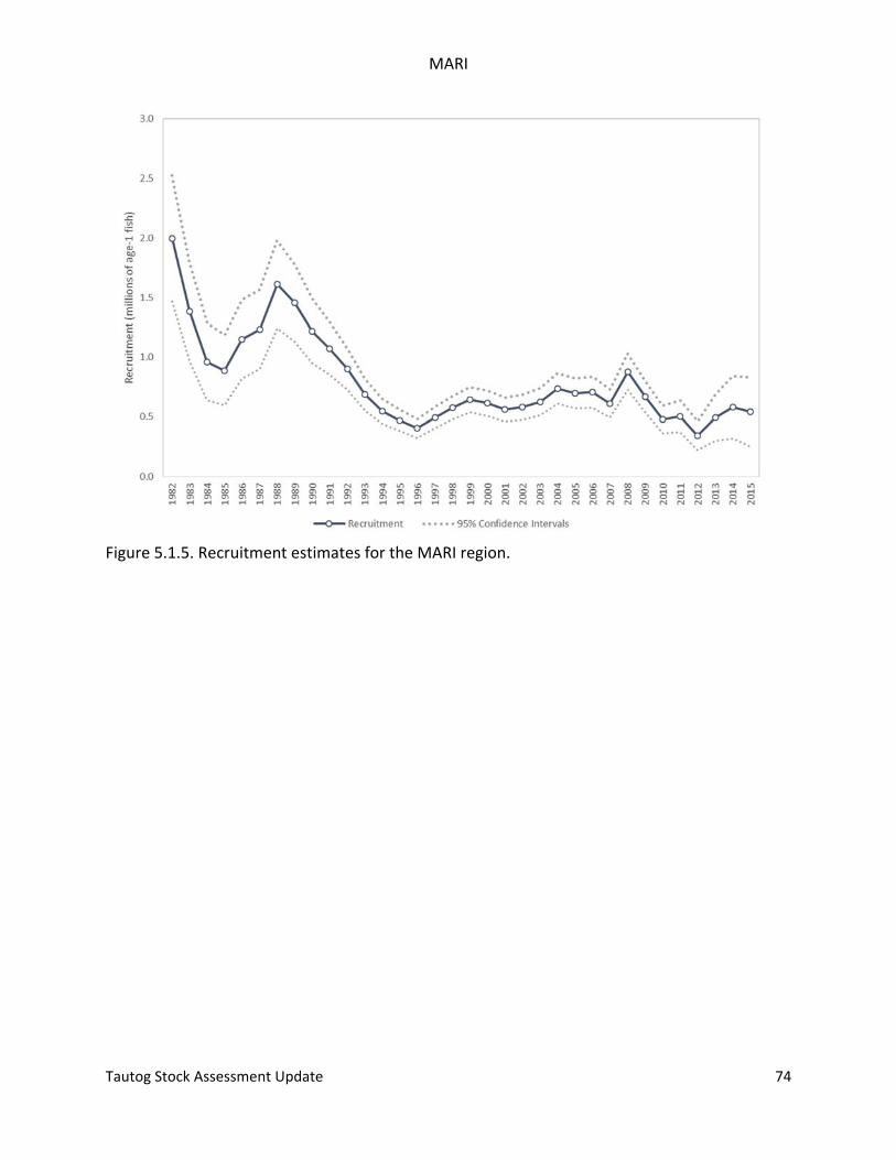
MARI
Tautog Stock Assessment Update 74
Figure 5.1.5. Recruitment estimates for the MARI region.
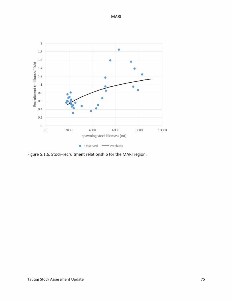
MARI
Tautog Stock Assessment Update 75
Figure 5.1.6. Stock‐recruitment relationship for the MARI region.
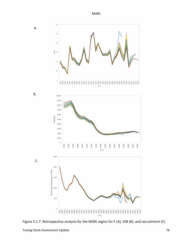
MARI
Tautog Stock Assessment Update 76
Figure 5.1.7. Retrospective analysis for the MARI region for F (A), SSB (B), and recruitment (C)
A.
B.
C.
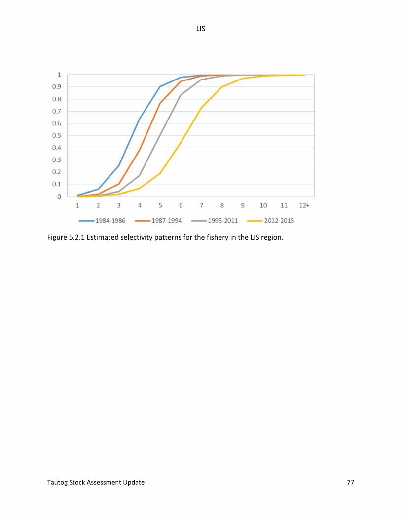
LIS
Tautog Stock Assessment Update 77
Figure 5.2.1 Estimated selectivity patterns for the fishery in the LIS region.
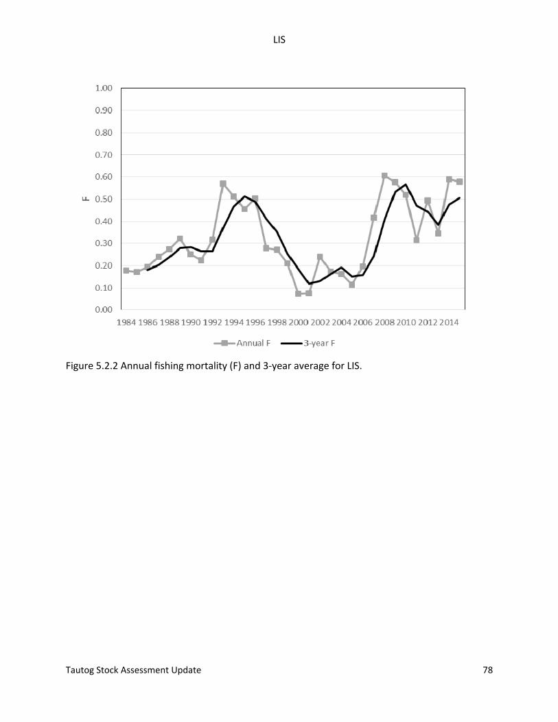
LIS
Tautog Stock Assessment Update 78
Figure 5.2.2 Annual fishing mortality (F) and 3‐year average for LIS.
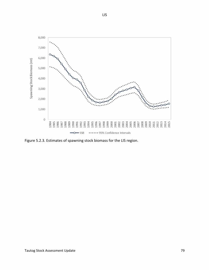
LIS
Tautog Stock Assessment Update 79
Figure 5.2.3. Estimates of spawning stock biomass for the LIS region.
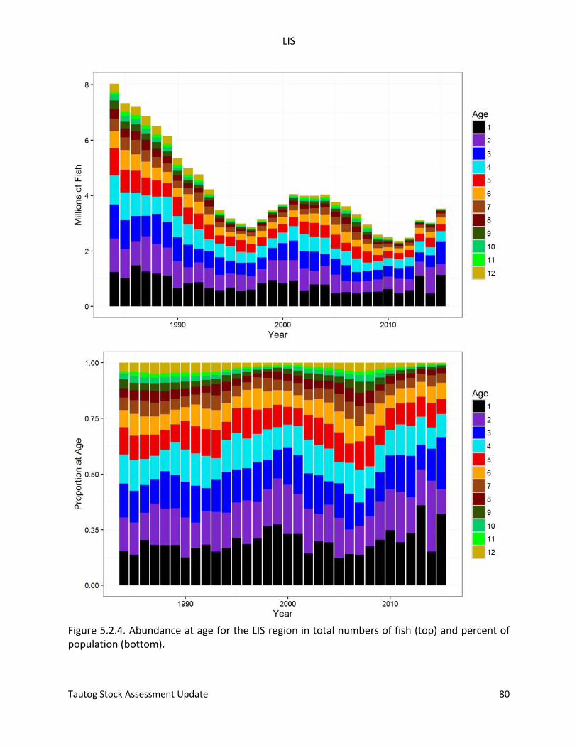
LIS
Tautog Stock Assessment Update 80
Figure 5.2.4. Abundance at age for the LIS region in total numbers of fish (top) and percent of population (bottom).
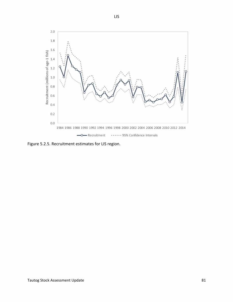
LIS
Tautog Stock Assessment Update 81
Figure 5.2.5. Recruitment estimates for LIS region.
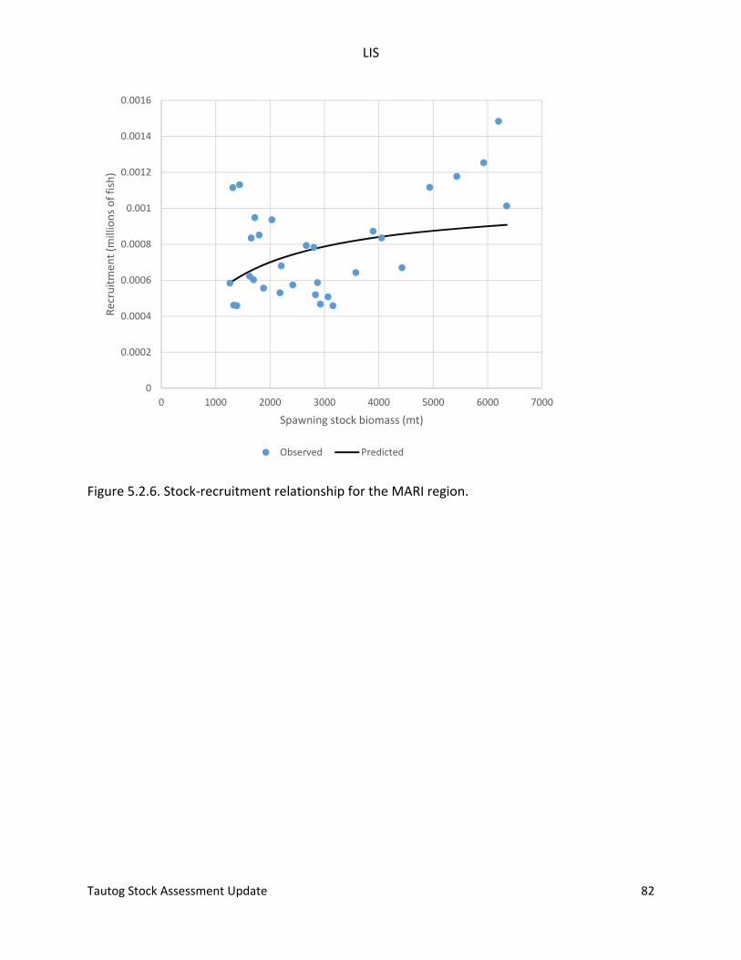
LIS
Tautog Stock Assessment Update 82
Figure 5.2.6. Stock‐recruitment relationship for the MARI region.
0
0.0002
0.0004
0.0006
0.0008
0.001
0.0012
0.0014
0.0016
0 1000 2000 3000 4000 5000 6000 7000
Recruitmen
t (m
illions of fish)
Spawning stock biomass (mt)
Observed Predicted
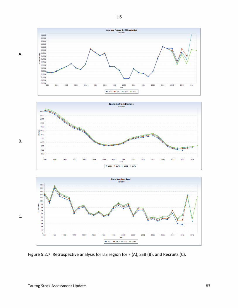
LIS
Tautog Stock Assessment Update 83
Figure 5.2.7. Retrospective analysis for LIS region for F (A), SSB (B), and Recruits (C).
A.
B.
C.
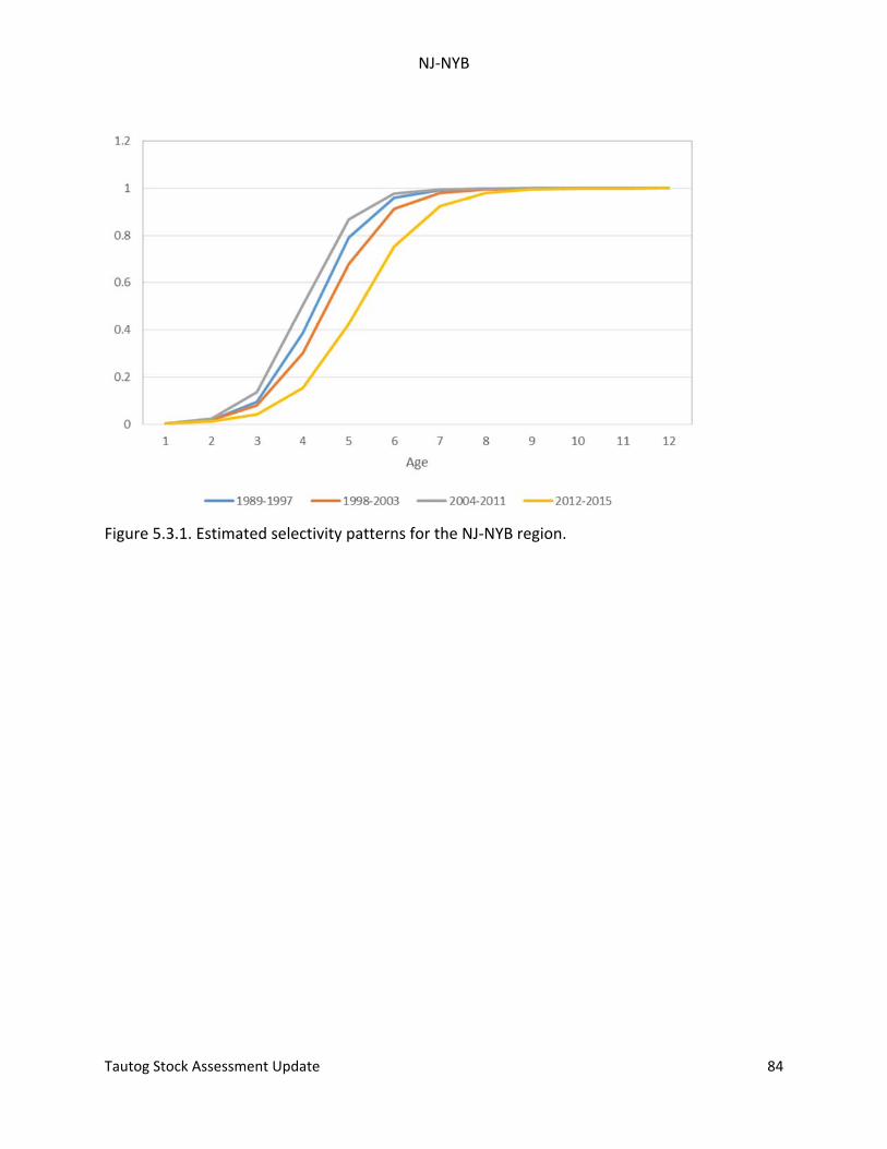
NJ‐NYB
Tautog Stock Assessment Update 84
Figure 5.3.1. Estimated selectivity patterns for the NJ‐NYB region.
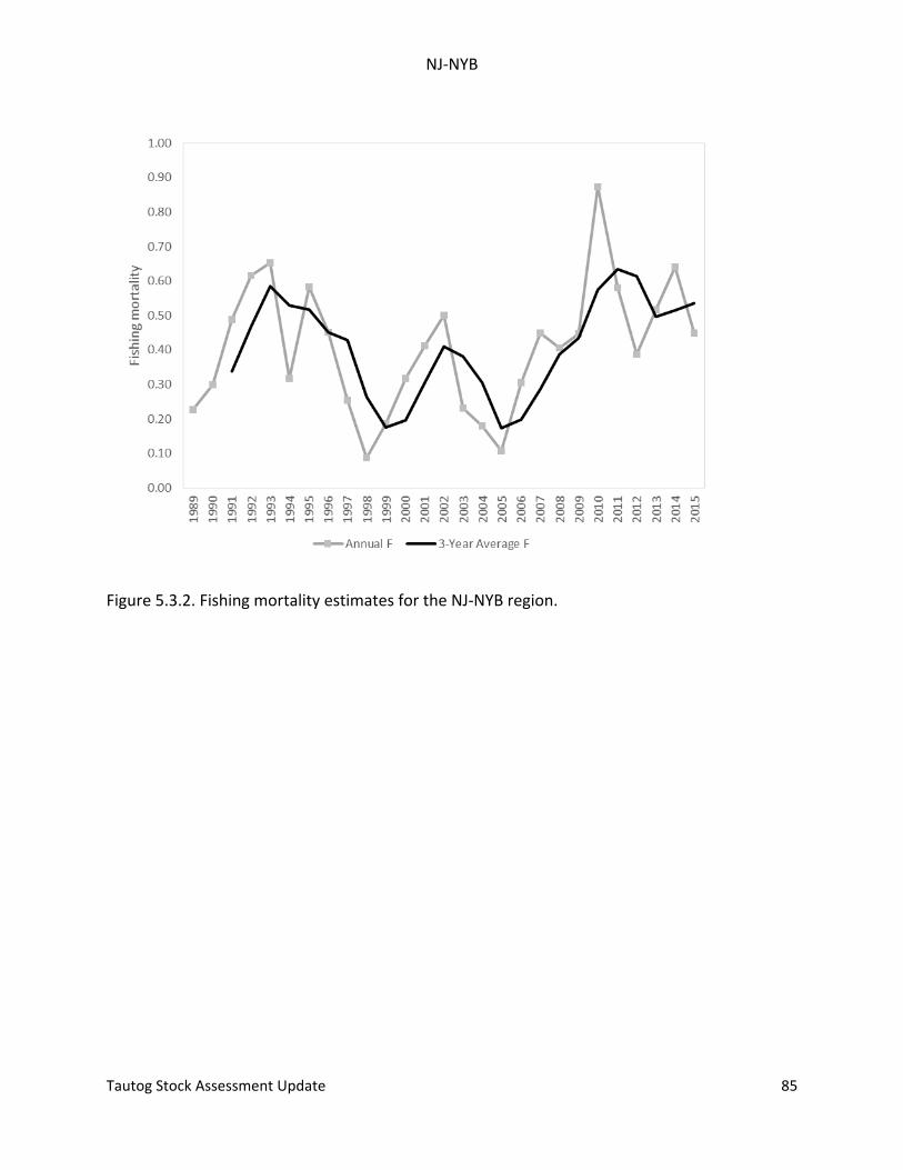
NJ‐NYB
Tautog Stock Assessment Update 85
Figure 5.3.2. Fishing mortality estimates for the NJ‐NYB region.
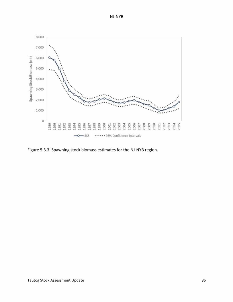
NJ‐NYB
Tautog Stock Assessment Update 86
Figure 5.3.3. Spawning stock biomass estimates for the NJ‐NYB region.
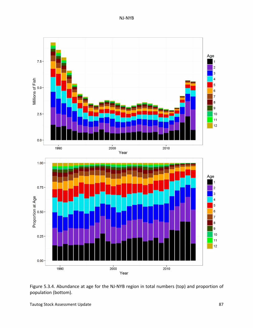
NJ‐NYB
Tautog Stock Assessment Update 87
Figure 5.3.4. Abundance at age for the NJ‐NYB region in total numbers (top) and proportion of population (bottom).
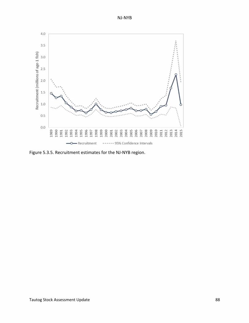
NJ‐NYB
Tautog Stock Assessment Update 88
Figure 5.3.5. Recruitment estimates for the NJ‐NYB region.
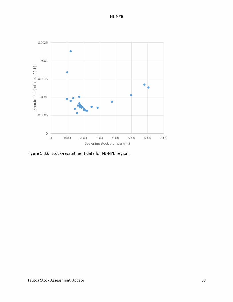
NJ‐NYB
Tautog Stock Assessment Update 89
Figure 5.3.6. Stock‐recruitment data for NJ‐NYB region.
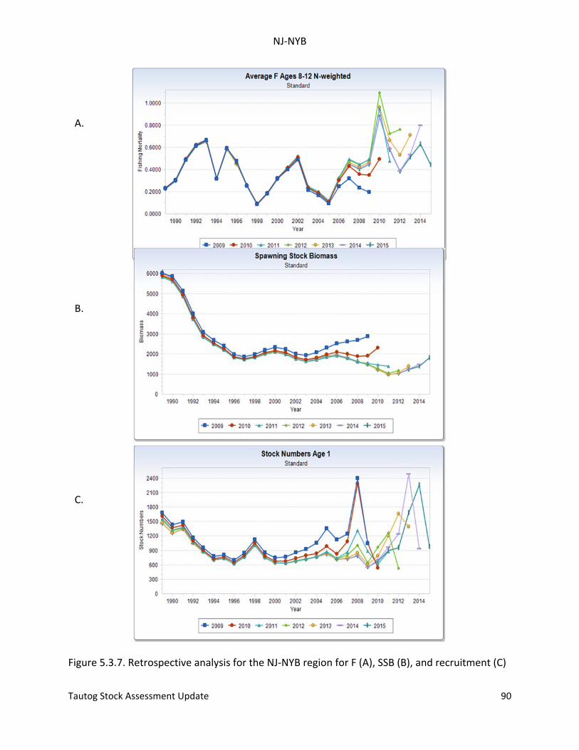
NJ‐NYB
Tautog Stock Assessment Update 90
Figure 5.3.7. Retrospective analysis for the NJ‐NYB region for F (A), SSB (B), and recruitment (C)
A.
B.
C.
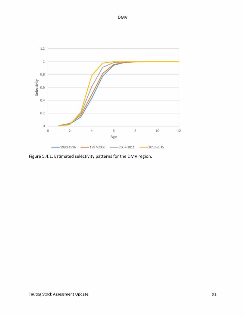
DMV
Tautog Stock Assessment Update 91
Figure 5.4.1. Estimated selectivity patterns for the DMV region.
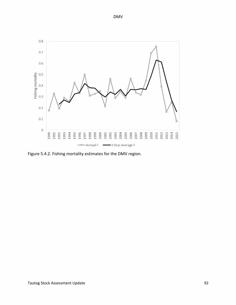
DMV
Tautog Stock Assessment Update 92
Figure 5.4.2. Fishing mortality estimates for the DMV region.
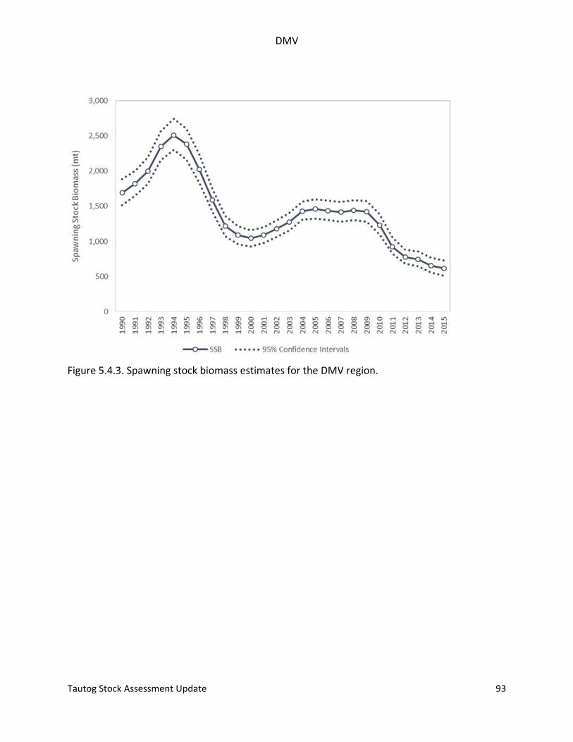
DMV
Tautog Stock Assessment Update 93
Figure 5.4.3. Spawning stock biomass estimates for the DMV region.
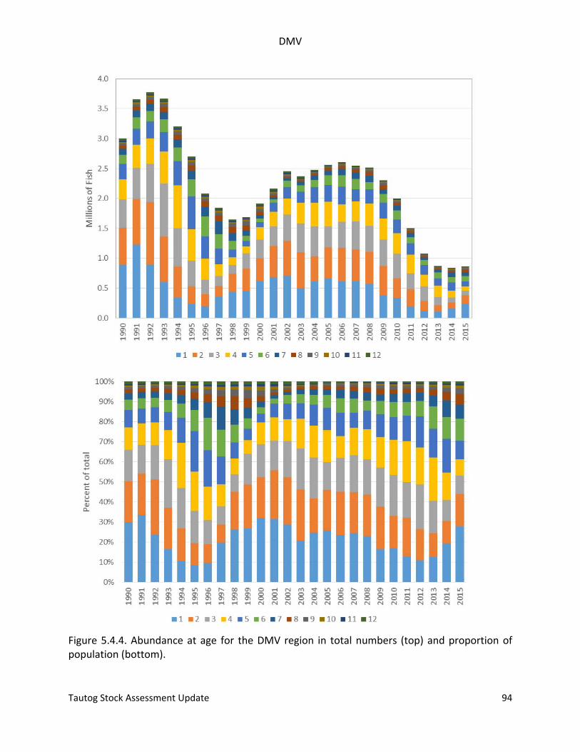
DMV
Tautog Stock Assessment Update 94
Figure 5.4.4. Abundance at age for the DMV region in total numbers (top) and proportion of population (bottom).
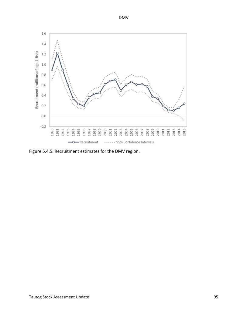
DMV
Tautog Stock Assessment Update 95
Figure 5.4.5. Recruitment estimates for the DMV region.
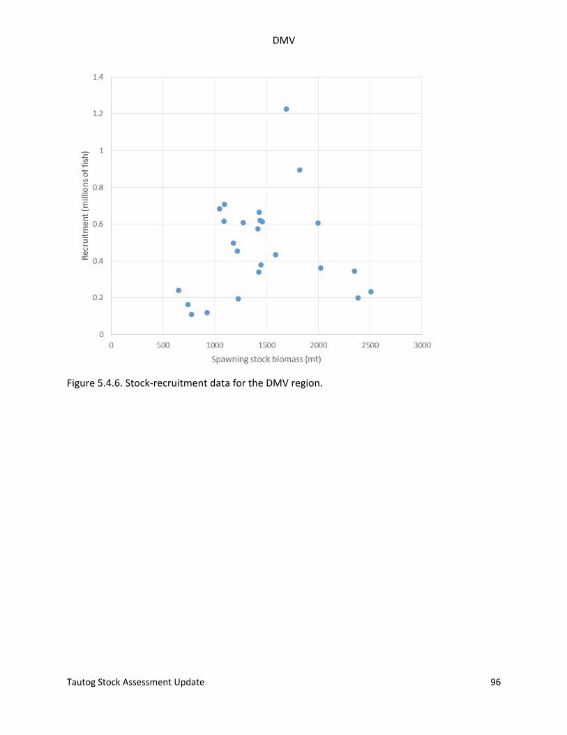
DMV
Tautog Stock Assessment Update 96
Figure 5.4.6. Stock‐recruitment data for the DMV region.
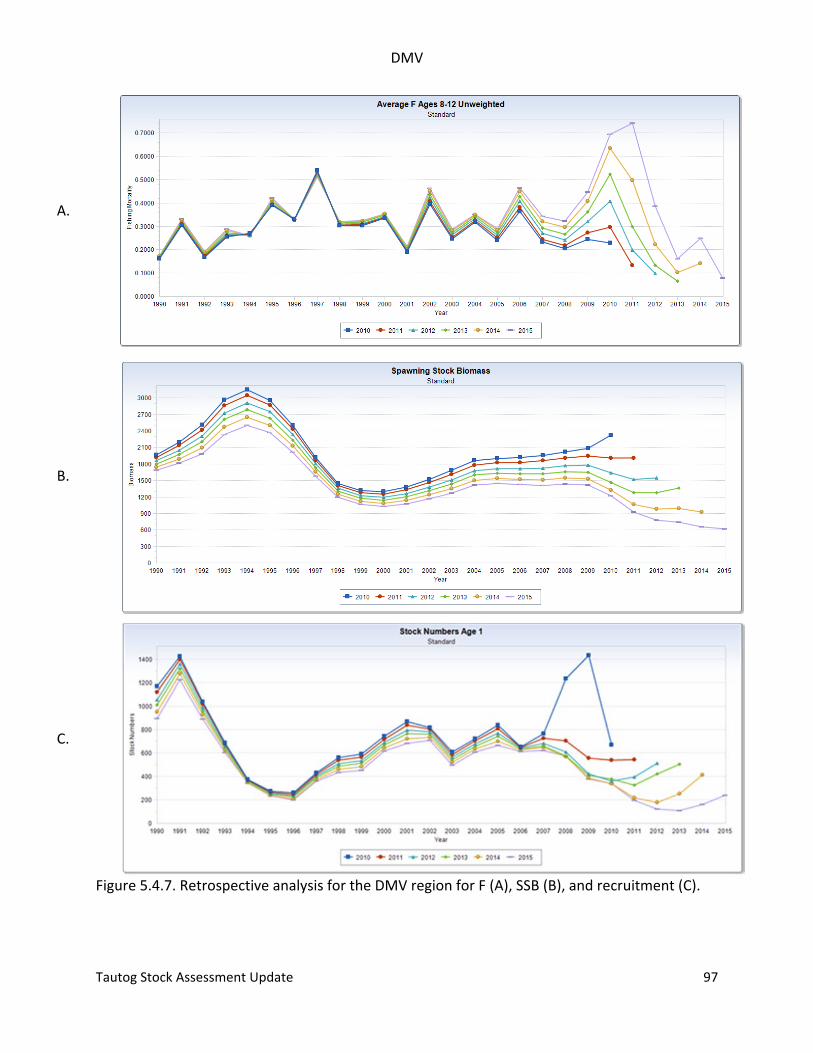
DMV
Tautog Stock Assessment Update 97
Figure 5.4.7. Retrospective analysis for the DMV region for F (A), SSB (B), and recruitment (C).
A.
B.
C.
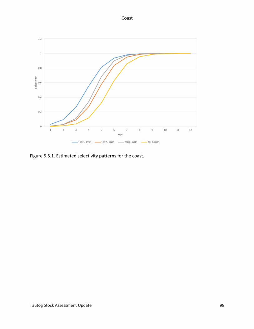
Coast
Tautog Stock Assessment Update 98
Figure 5.5.1. Estimated selectivity patterns for the coast.
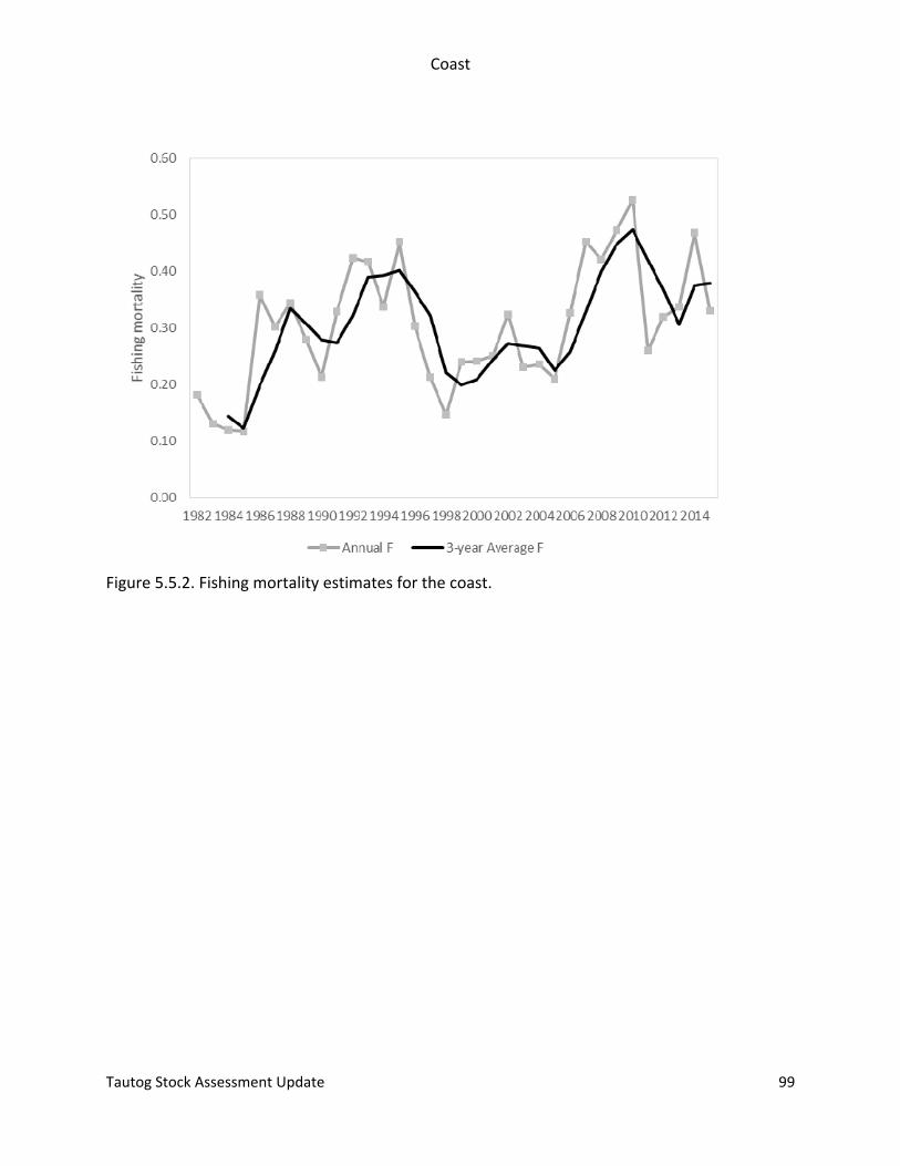
Coast
Tautog Stock Assessment Update 99
Figure 5.5.2. Fishing mortality estimates for the coast.
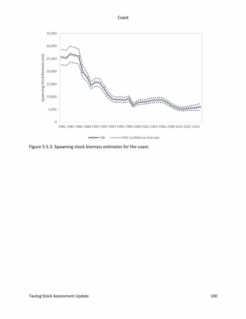
Coast
Tautog Stock Assessment Update 100
Figure 5.5.3. Spawning stock biomass estimates for the coast.
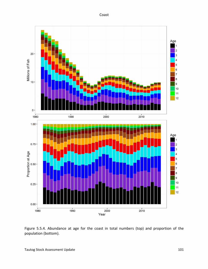
Coast
Tautog Stock Assessment Update 101
Figure 5.5.4. Abundance at age for the coast in total numbers (top) and proportion of the population (bottom).
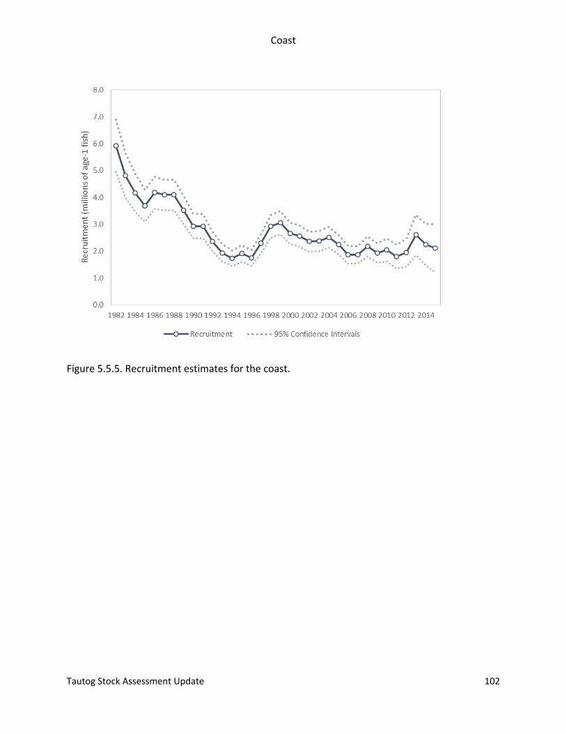
Coast
Tautog Stock Assessment Update 102
Figure 5.5.5. Recruitment estimates for the coast.
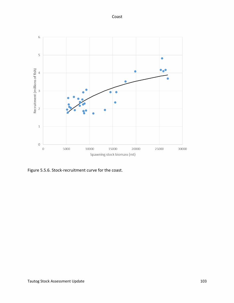
Coast
Tautog Stock Assessment Update 103
Figure 5.5.6. Stock‐recruitment curve for the coast.
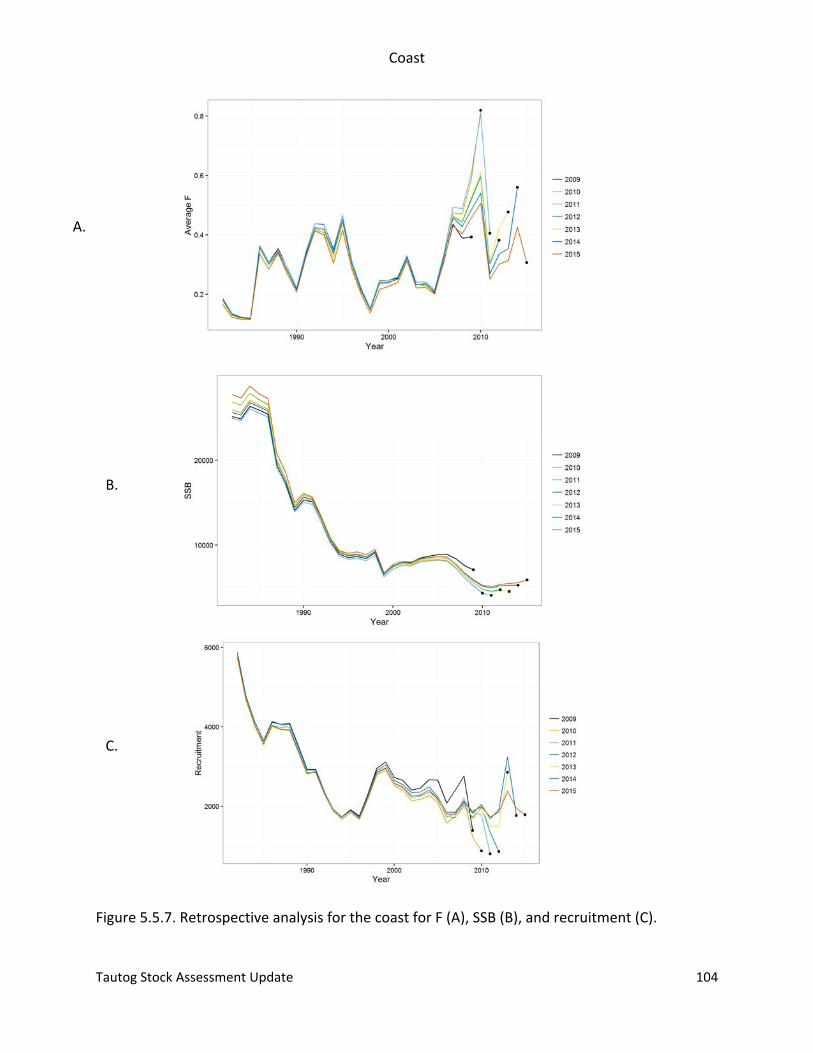
Coast
Tautog Stock Assessment Update 104
Figure 5.5.7. Retrospective analysis for the coast for F (A), SSB (B), and recruitment (C).
C.
B.
A.
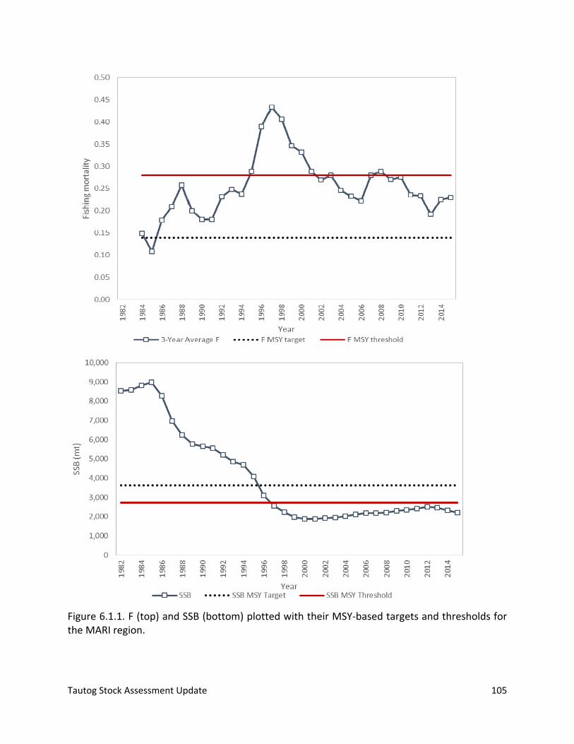
Tautog Stock Assessment Update 105
Figure 6.1.1. F (top) and SSB (bottom) plotted with their MSY‐based targets and thresholds for the MARI region.
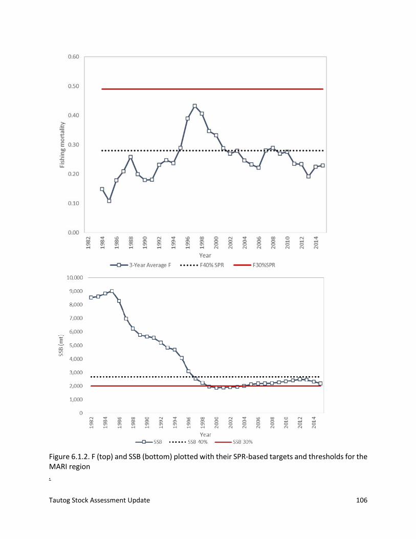
Tautog Stock Assessment Update 106
Figure 6.1.2. F (top) and SSB (bottom) plotted with their SPR‐based targets and thresholds for the MARI region .
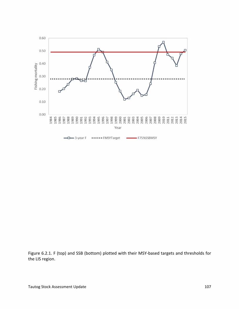
Tautog Stock Assessment Update 107
Figure 6.2.1. F (top) and SSB (bottom) plotted with their MSY‐based targets and thresholds for the LIS region.
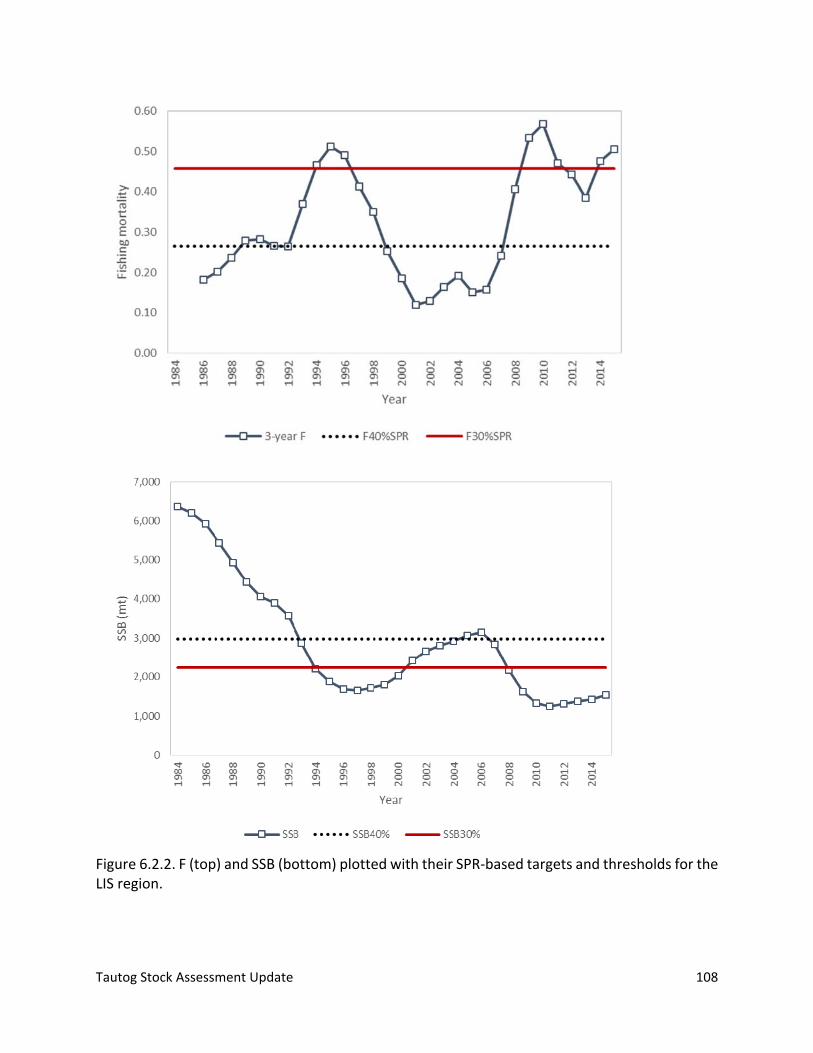
Tautog Stock Assessment Update 108
Figure 6.2.2. F (top) and SSB (bottom) plotted with their SPR‐based targets and thresholds for the LIS region.
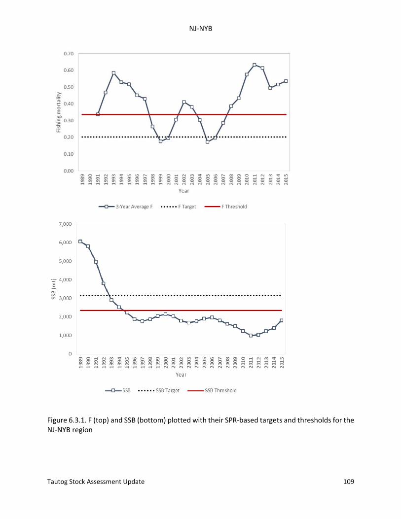
NJ‐NYB
Tautog Stock Assessment Update 109
Figure 6.3.1. F (top) and SSB (bottom) plotted with their SPR‐based targets and thresholds for the NJ‐NYB region
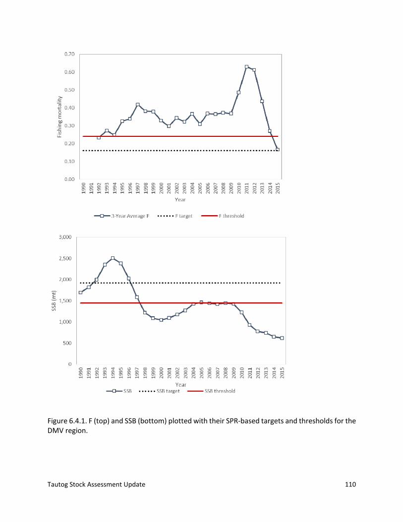
Tautog Stock Assessment Update 110
Figure 6.4.1. F (top) and SSB (bottom) plotted with their SPR‐based targets and thresholds for the DMV region.
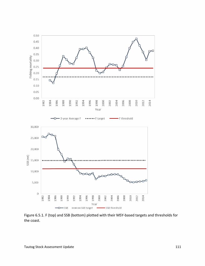
Tautog Stock Assessment Update 111
Figure 6.5.1. F (top) and SSB (bottom) plotted with their MSY‐based targets and thresholds for
the coast.
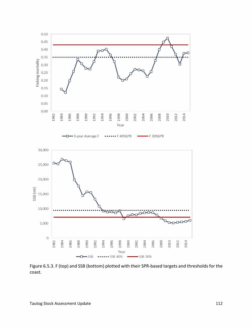
Tautog Stock Assessment Update 112
Figure 6.5.3. F (top) and SSB (bottom) plotted with their SPR‐based targets and thresholds for the coast.
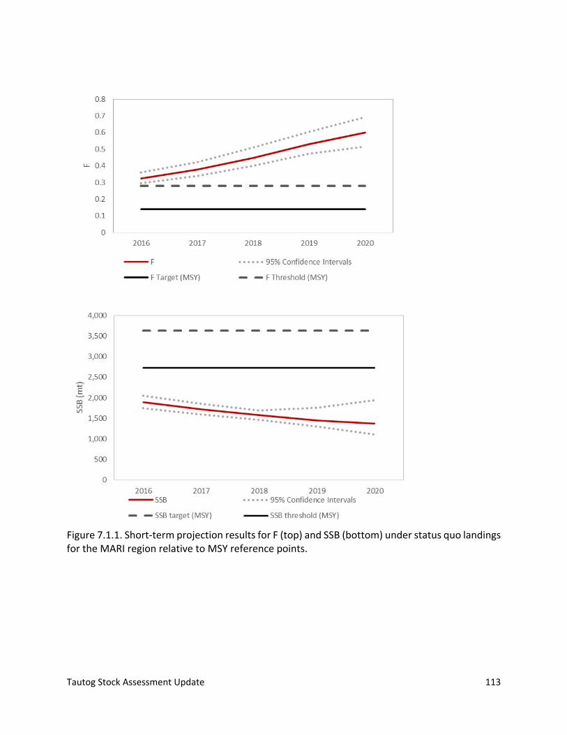
Tautog Stock Assessment Update 113
Figure 7.1.1. Short‐term projection results for F (top) and SSB (bottom) under status quo landings for the MARI region relative to MSY reference points.
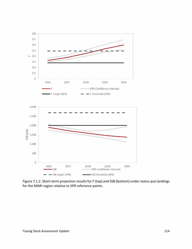
Tautog Stock Assessment Update 114
Figure 7.1.2. Short‐term projection results for F (top) and SSB (bottom) under status quo landings for the MARI region relative to SPR reference points.
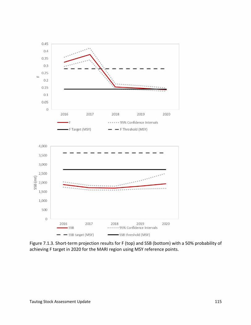
Tautog Stock Assessment Update 115
Figure 7.1.3. Short‐term projection results for F (top) and SSB (bottom) with a 50% probability of achieving F target in 2020 for the MARI region using MSY reference points.
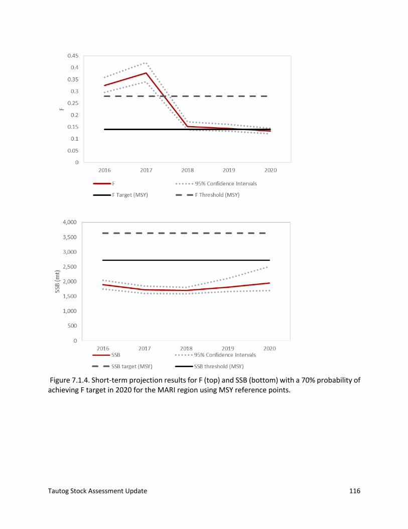
Tautog Stock Assessment Update 116
Figure 7.1.4. Short‐term projection results for F (top) and SSB (bottom) with a 70% probability of achieving F target in 2020 for the MARI region using MSY reference points.
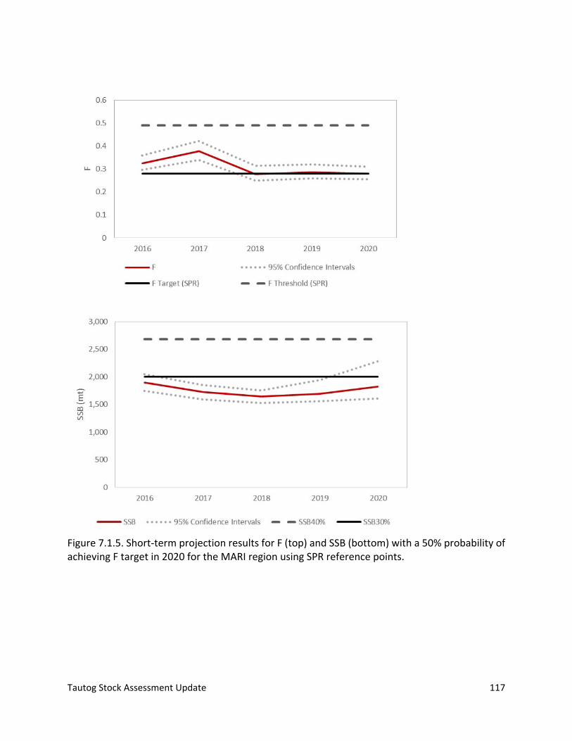
Tautog Stock Assessment Update 117
Figure 7.1.5. Short‐term projection results for F (top) and SSB (bottom) with a 50% probability of achieving F target in 2020 for the MARI region using SPR reference points.
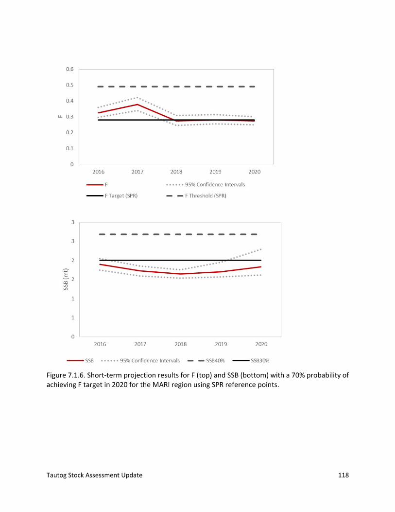
Tautog Stock Assessment Update 118
Figure 7.1.6. Short‐term projection results for F (top) and SSB (bottom) with a 70% probability of achieving F target in 2020 for the MARI region using SPR reference points.
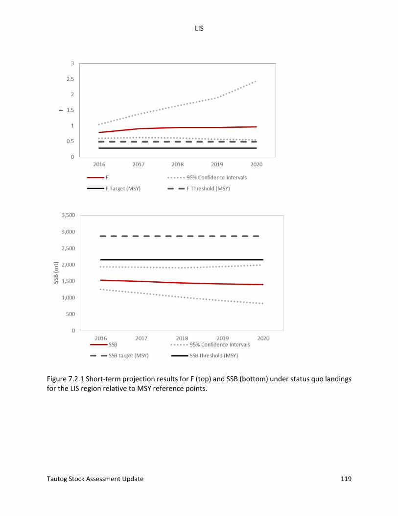
LIS
Tautog Stock Assessment Update 119
Figure 7.2.1 Short‐term projection results for F (top) and SSB (bottom) under status quo landings for the LIS region relative to MSY reference points.
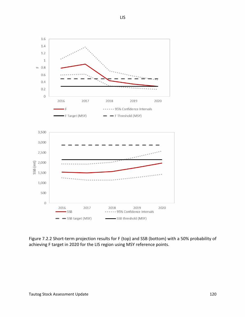
LIS
Tautog Stock Assessment Update 120
Figure 7.2.2 Short‐term projection results for F (top) and SSB (bottom) with a 50% probability of achieving F target in 2020 for the LIS region using MSY reference points.
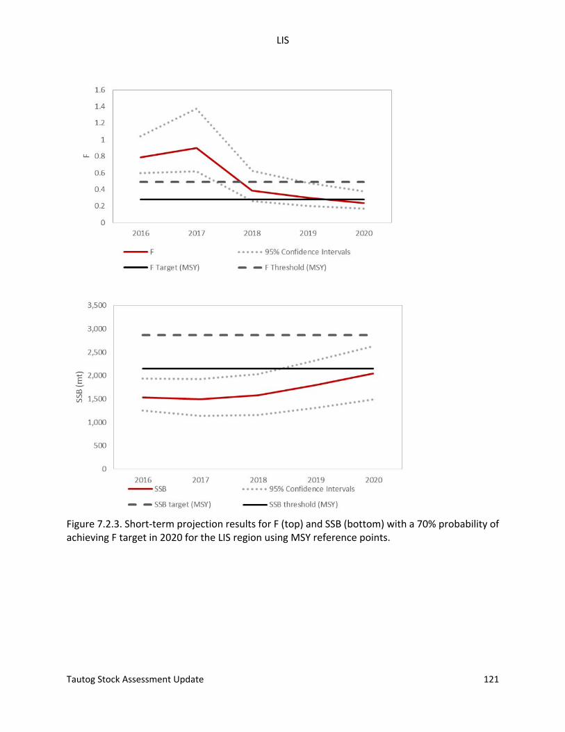
LIS
Tautog Stock Assessment Update 121
Figure 7.2.3. Short‐term projection results for F (top) and SSB (bottom) with a 70% probability of achieving F target in 2020 for the LIS region using MSY reference points.
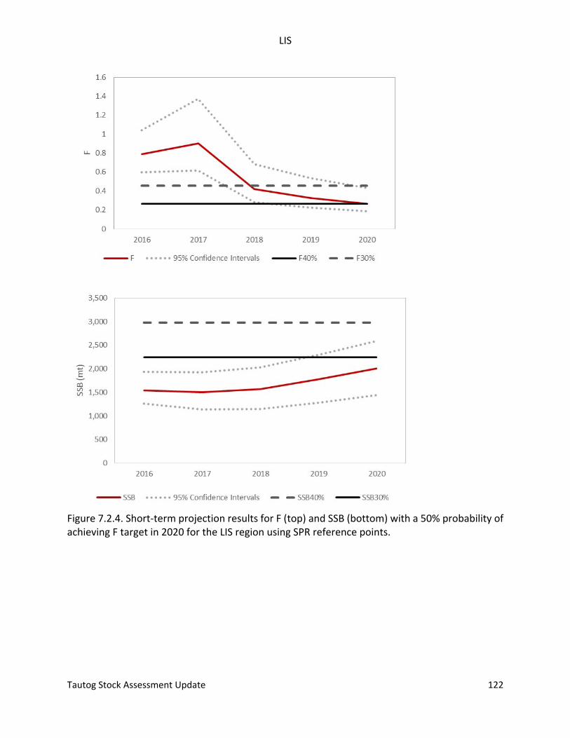
LIS
Tautog Stock Assessment Update 122
Figure 7.2.4. Short‐term projection results for F (top) and SSB (bottom) with a 50% probability of achieving F target in 2020 for the LIS region using SPR reference points.
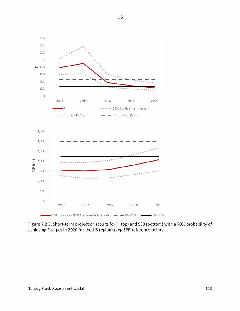
LIS
Tautog Stock Assessment Update 123
Figure 7.2.5. Short‐term projection results for F (top) and SSB (bottom) with a 70% probability of achieving F target in 2020 for the LIS region using SPR reference points.
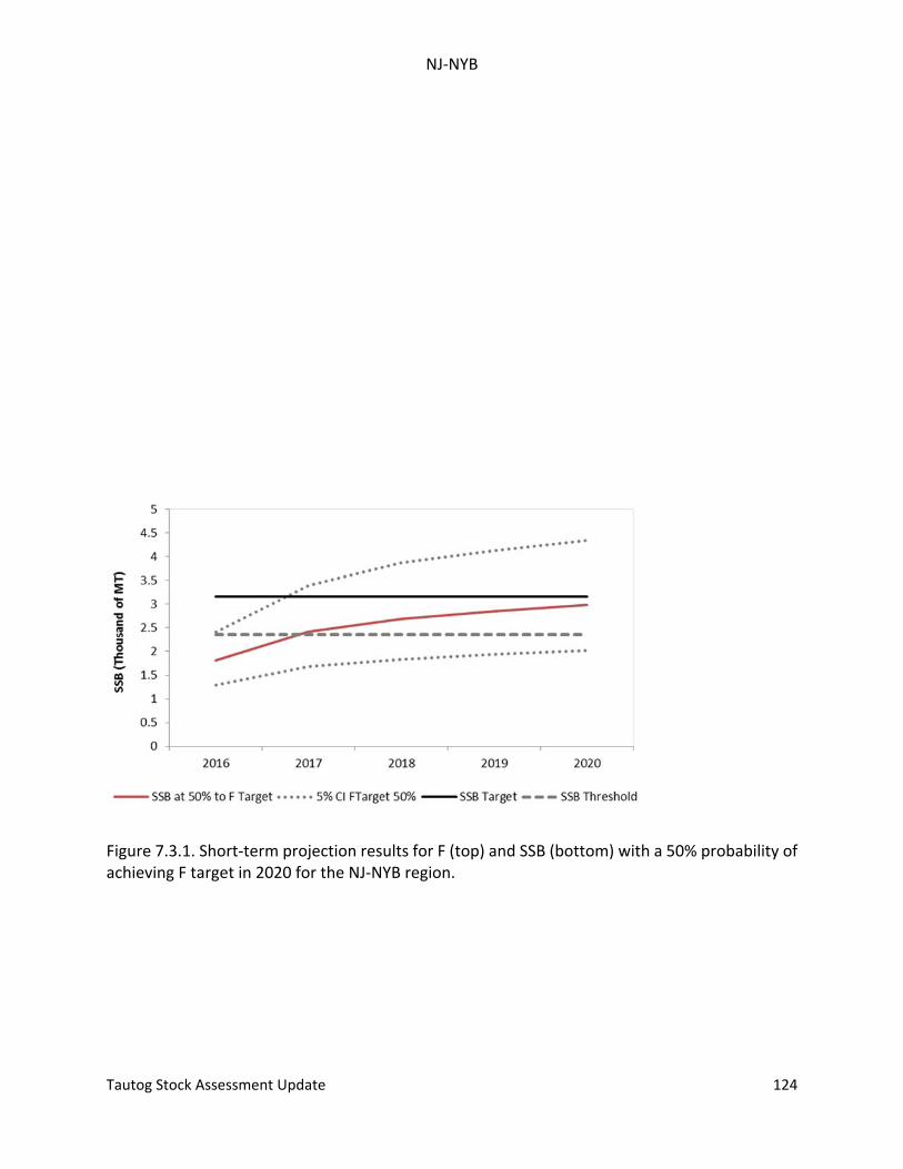
NJ‐NYB
Tautog Stock Assessment Update 124
Figure 7.3.1. Short‐term projection results for F (top) and SSB (bottom) with a 50% probability of achieving F target in 2020 for the NJ‐NYB region.
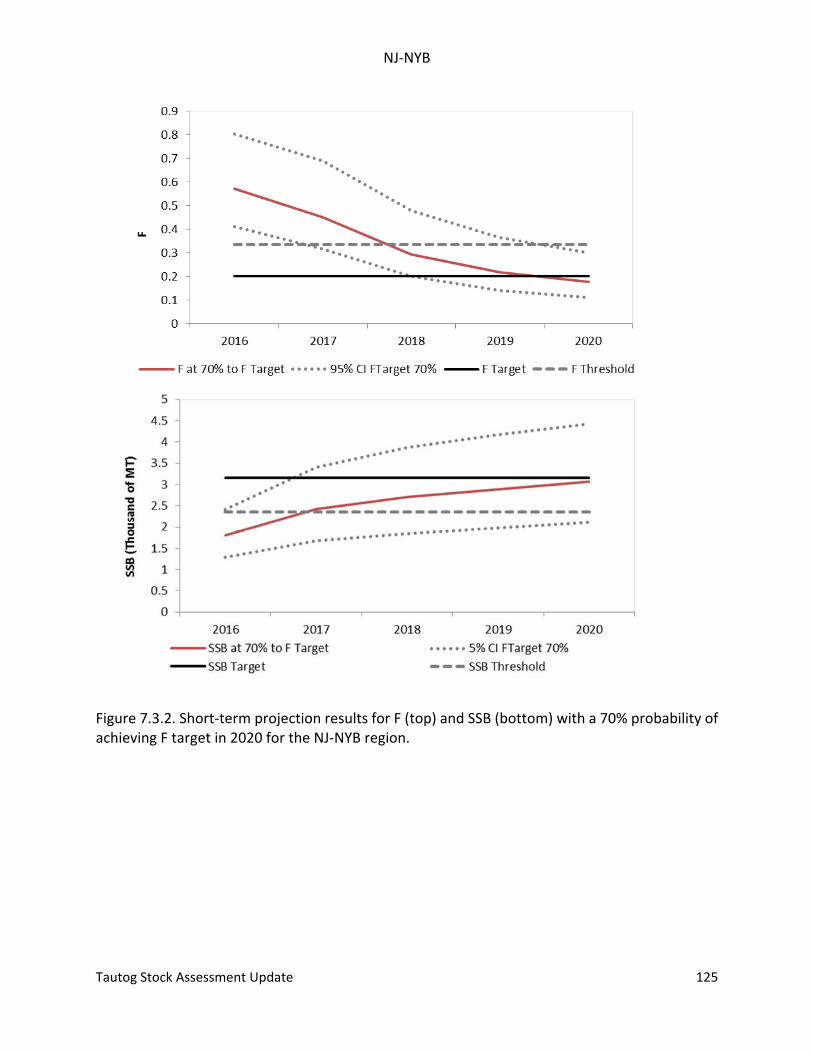
NJ‐NYB
Tautog Stock Assessment Update 125
Figure 7.3.2. Short‐term projection results for F (top) and SSB (bottom) with a 70% probability of achieving F target in 2020 for the NJ‐NYB region.
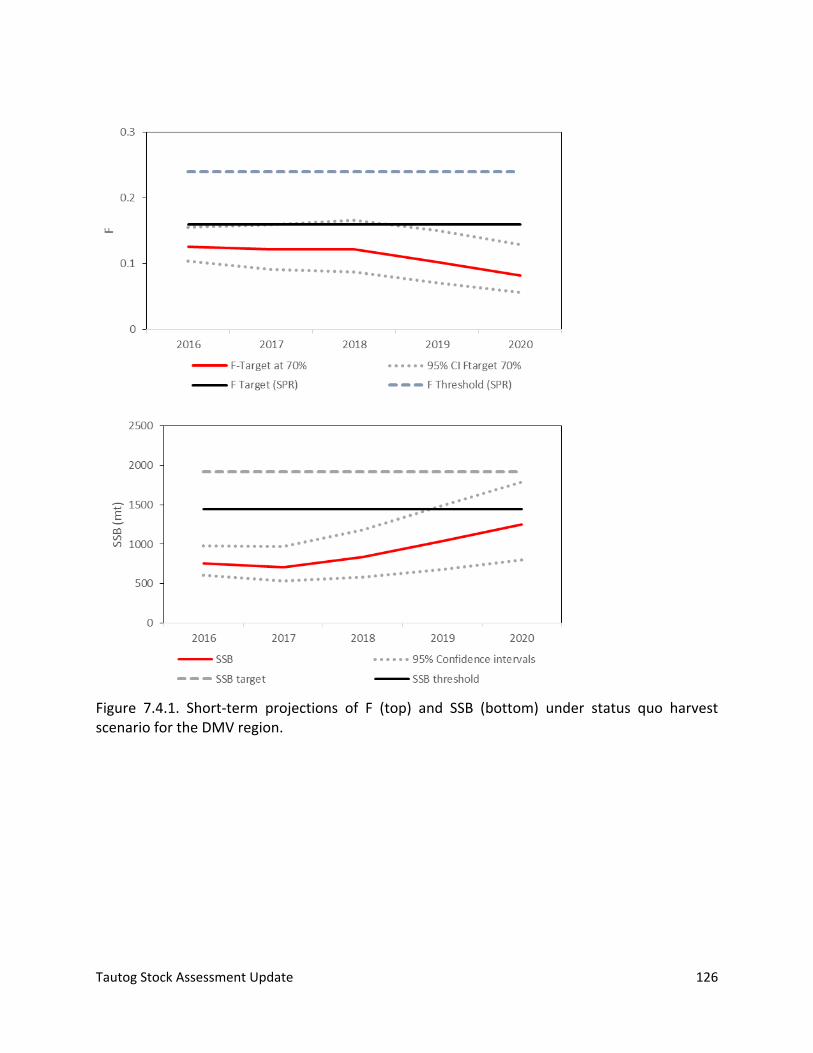
Tautog Stock Assessment Update 126
Figure 7.4.1. Short‐term projections of F (top) and SSB (bottom) under status quo harvest scenario for the DMV region.
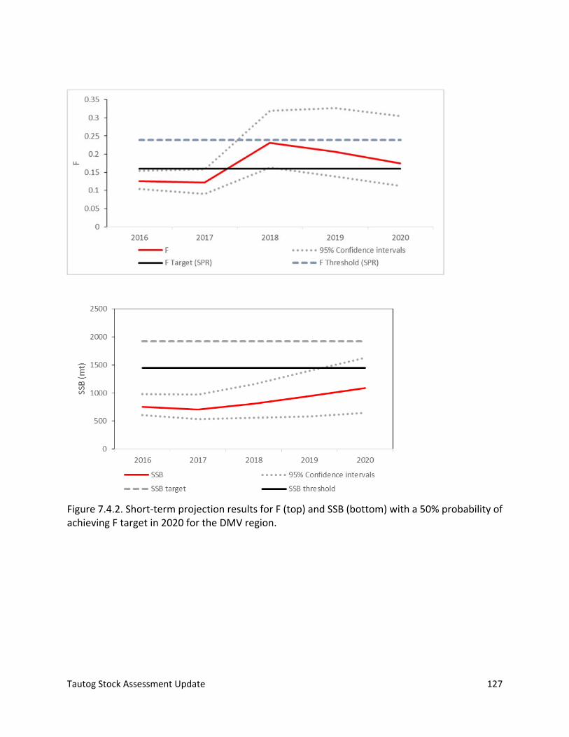
Tautog Stock Assessment Update 127
Figure 7.4.2. Short‐term projection results for F (top) and SSB (bottom) with a 50% probability of achieving F target in 2020 for the DMV region.
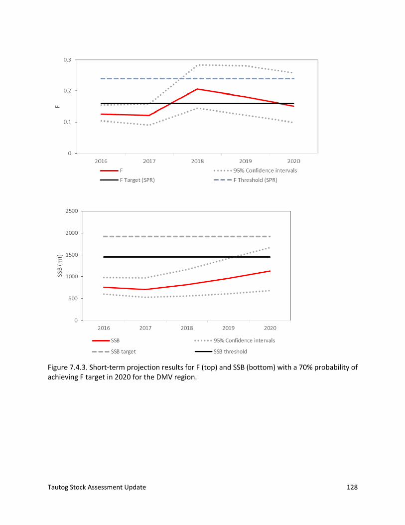
Tautog Stock Assessment Update 128
Figure 7.4.3. Short‐term projection results for F (top) and SSB (bottom) with a 70% probability of achieving F target in 2020 for the DMV region.
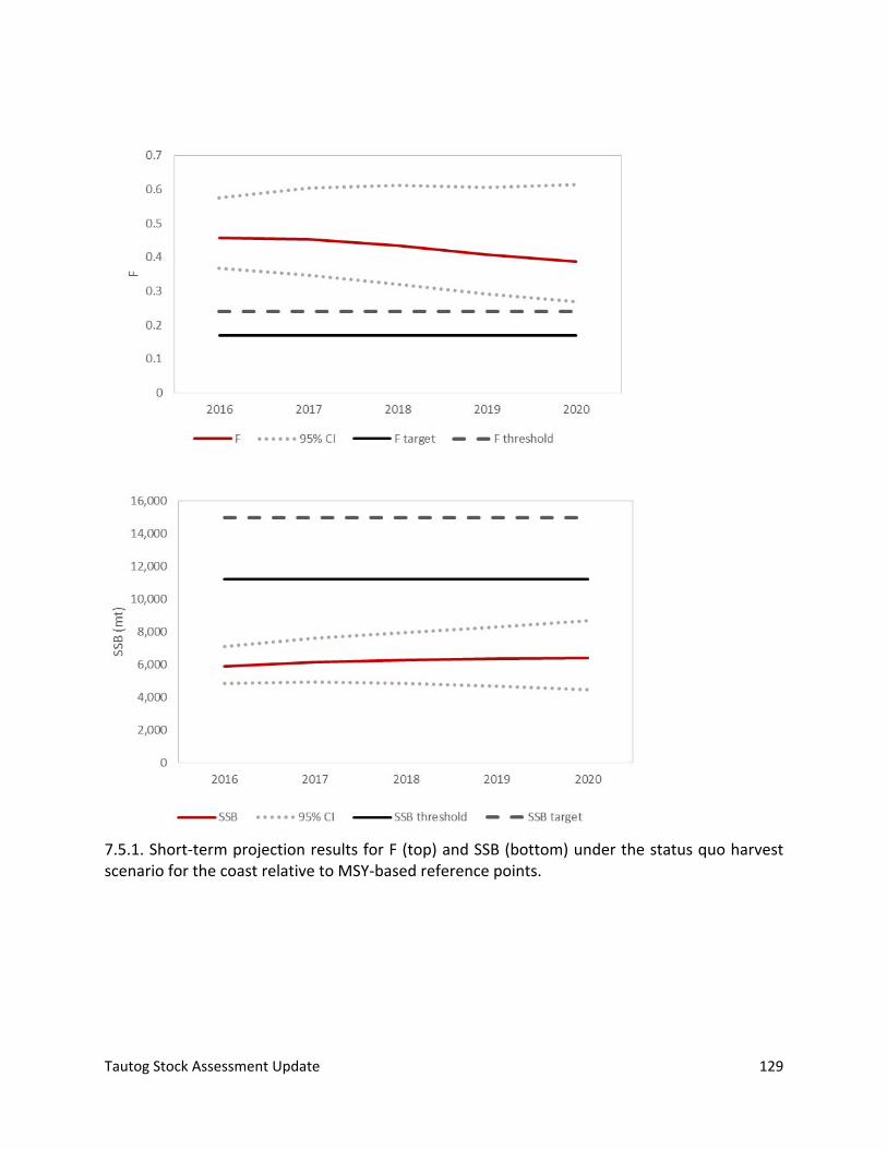
Tautog Stock Assessment Update 129
7.5.1. Short‐term projection results for F (top) and SSB (bottom) under the status quo harvest scenario for the coast relative to MSY‐based reference points.
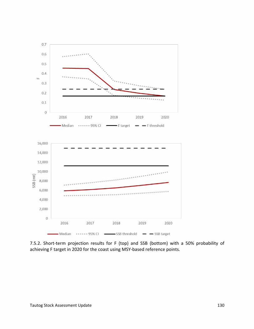
Tautog Stock Assessment Update 130
7.5.2. Short‐term projection results for F (top) and SSB (bottom) with a 50% probability of achieving F target in 2020 for the coast using MSY‐based reference points.
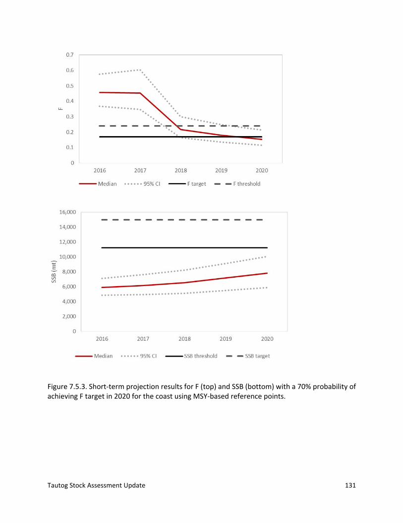
Tautog Stock Assessment Update 131
Figure 7.5.3. Short‐term projection results for F (top) and SSB (bottom) with a 70% probability of achieving F target in 2020 for the coast using MSY‐based reference points.
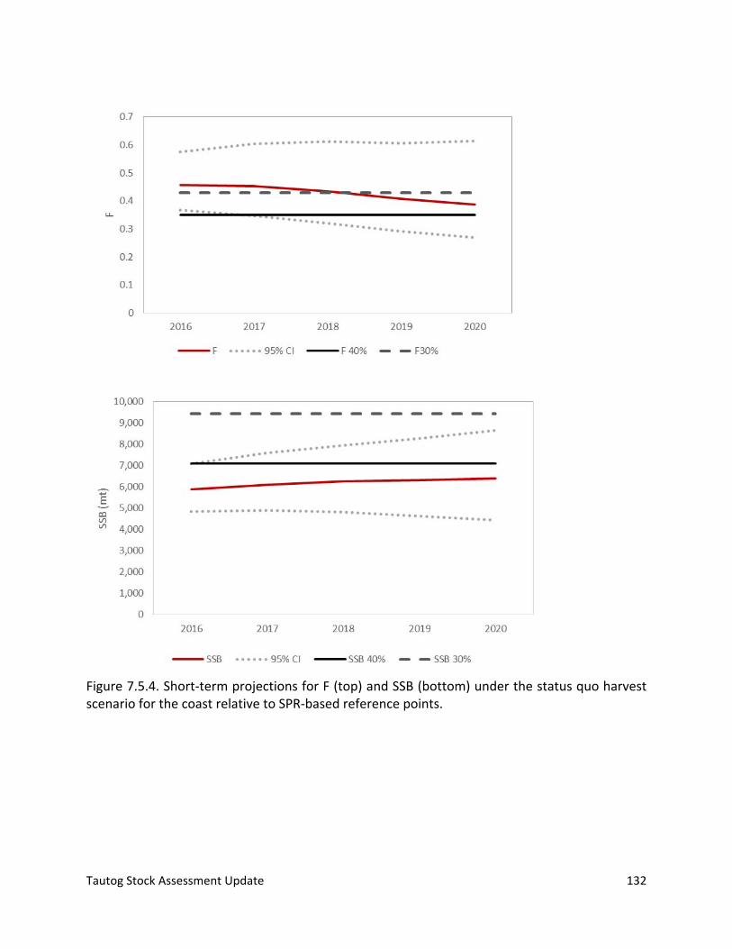
Tautog Stock Assessment Update 132
Figure 7.5.4. Short‐term projections for F (top) and SSB (bottom) under the status quo harvest scenario for the coast relative to SPR‐based reference points.
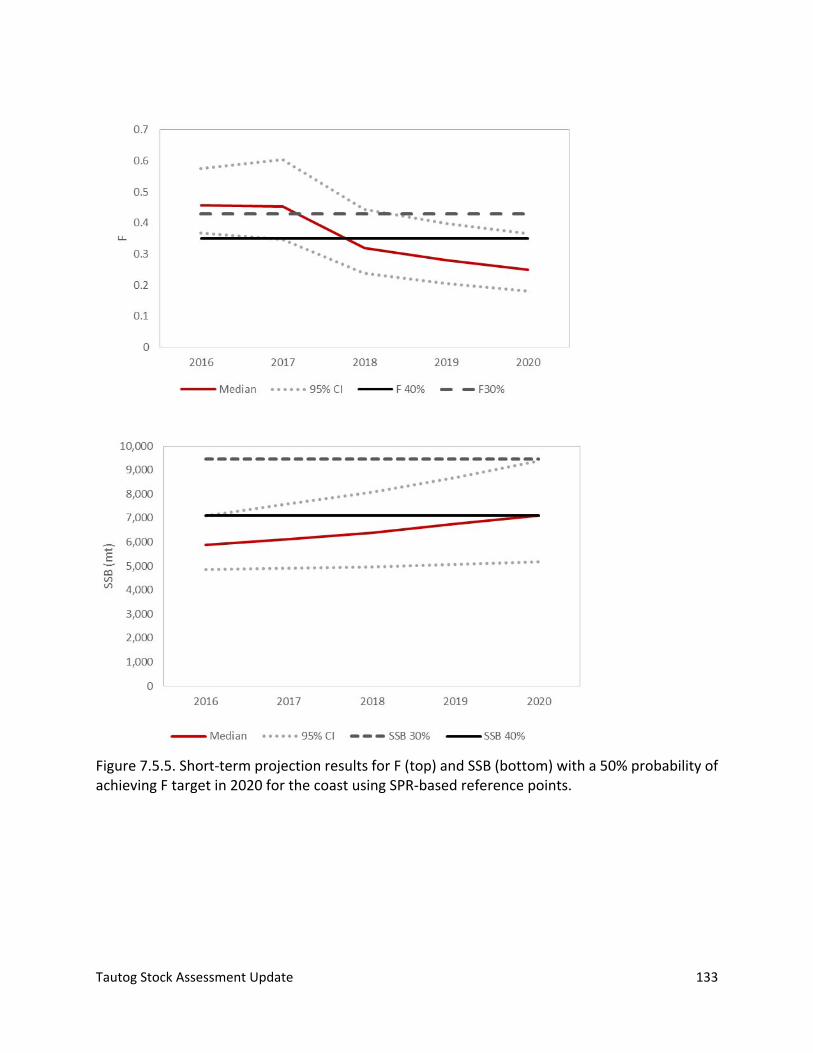
Tautog Stock Assessment Update 133
Figure 7.5.5. Short‐term projection results for F (top) and SSB (bottom) with a 50% probability of achieving F target in 2020 for the coast using SPR‐based reference points.
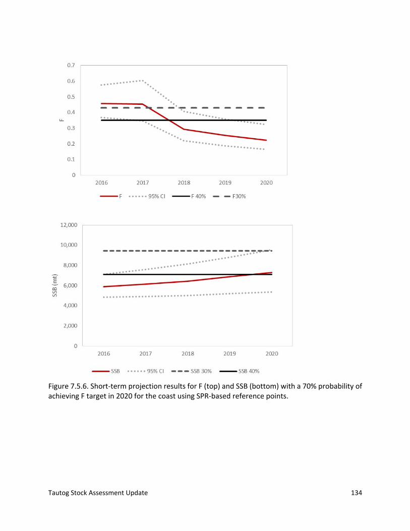
Tautog Stock Assessment Update 134
Figure 7.5.6. Short‐term projection results for F (top) and SSB (bottom) with a 70% probability of achieving F target in 2020 for the coast using SPR‐based reference points.