Embed Size (px)
Citation preview

Stellar magnetic activityfrom the photosphere to circumstellar
disks
Dissertationzur Erlangung des Doktorgrades
des Departments Physikder Universitat Hamburg
vorgelegt von
Stefan Czeslaaus Hamburg
Hamburg2010

Gutachter der Dissertation: Prof. Dr. J. H. M. M. SchmittProf. Dr. E. D. Feigelson
Gutachter der Disputation: Prof. Dr. P. HauschildtProf. Dr. D. Horns
Datum der Disputation: 11.11.2010
Vorsitzender des Prufungsausschusses: Dr. R. Baade
Vorsitzender des Promotionsausschusses: Prof. Dr. J. Bartels
Dekan der MIN Fakultat: Prof. Dr. H. Graener

ZusammenfassungDie Erforschung der Sonnenaktivitat gehort zu den altesten Zweigen der Astronomie. DerFortschritt der Beobachtungstechnik ermoglichte eine Ausdehnung der Aktivitatsstudienweit uber die Sonne hinaus in den Bereich der stellaren Aktivitat. Die Entwicklung vonsatellitengestutzten Instrumenten erlaubte den Astronomen den Zugriff auf Spektralberei-che, die von der Erdatmosphare verdeckt werden. Die Erforschung des so erschlossenenRontgenhimmels gestattet grundlegende Einsichten in die Natur stellarer magnetischer Ak-tivitat, die besonders wertvoll fur das Studium junger Sterne sind. Mit der Entdeckung desersten extrasolaren Planeten vor 15 Jahren begann der rasante Aufstieg des bis dato kleinen,diesen Objekten gewidmeten, Forschungsbereichs zu einem der großten und aktivsten Zweigeder Astronomie.
In der vorliegenden Arbeit werden unterschiedliche Aspekte stellarer Aktivitat unter-sucht. Die Themen reichen von dem klassischen Feld der Sternenflecken uber die Erforschungzirkumstellaren Materials mittels reprozessierter Rontgenstrahlung bis hin zur magnetischenAktivitat substellarer Objekte. Die Daten hierzu stammen von CoRoT im Optischen undvon Chandra im Rontgenbereich.
Zu Beginn wird die optische Lichtkurve des sonnenahnlichen, jedoch jungen SternsCoRoT-2a im Hinblick auf den Einfluss von Aktivitat auf die Transitlichtkurven eines be-deckenden, jupiterahnlichen Planeten untersucht. Des Weiteren wird eine neue Lichtkurven-inversionstechnik angewandt, um die Helligkeitsverteilung auf dem Stern zu rekonstruieren.
Stellare Aktivitat hat einen signifikanten Effekt auf die Transitlichtkurven, der bei genau-er Bestimmung der Planetenparameter nicht vernachlassigt werden sollte. Wir waren in derLage, die Oberflachenhelligkeitsverteilung des Sterns uber ein halbes Jahr hinweg in zwei,durch die Bedeckung des Planeten definierten, Bereichen zu rekonstruieren. Die zugehorigenKarten zeigen einen Stern mit zwei aktiven Langen auf gegenuberliegenden Hemispharen.
Anschließend werden Rontgenquellen einer Sternentstehungsregion im Orion untersucht,die im Rahmen des Chandra Orion Ultradeep Project beobachtet wurden. In den Quellenwird nach der Fe Kα I Fluoreszenzlinie gesucht und gegebenenfalls ihr Zeitverhalten analy-siert. Die vorherrschende Meinung ist, dass die Fe Kα I Linienemission auf Photoionisationin beleuchteten zirkumstellaren Scheiben zuruckzufuhren ist. Dieses Szenario kann mittelsdes Zeitverhaltens der Linienemission getestet werden.
Die Analyse liefert 23 Quellen, die signifikante Fe Kα I Linienemission zeigen. Diezeitliche Variabilitat der Fe Kα I Linie weist eine große Vielfalt auf. Einige Beobachtungenscheinen der weitverbreiteten These der Anregung durch Photoionisation zu widersprechen,die trotzdem die plausibelste Erklarung fur den Ursprung der Linie darstellt, wenn komplexeGeometrien in Erwagung gezogen werden.
Im letzten Teil der Arbeit wird uber die Rontgendetektion des ersten bedeckenden PaaresBrauner Zwerge berichtet, die auf der Massenskala den Platz zwischen Planeten und Sterneneinnehmen. Das untersuchte System ist das erste, in dem die Parameter von BraunenZwergen genau bestimmt werden konnen, und nimmt somit eine Schlusselstellung in derErforschung der fruhen Entwicklung und Aktivitat von massearmen Objekten ein.
Die im Rahmen dieser Arbeit prasentierten Studien demonstrieren die enorme Aus-sagekraft von Lichtkurvenanalysen. Wahrend die Analyse der Fe Kα I Linie in stellarenQuellen bereits an die Grenzen des momentan verfugbaren Instrumentariums fuhrt, birgtdie Analyse von optischen Helligkeitsverlaufen noch großes Potential, da zur Zeit tausendehochwertiger Lichtkurven von den Weltraumobservatorien CoRoT und Kepler beobachtetwerden.


Abstract
The study of solar activity is among the oldest branches of astronomy. With the inventionof new observation techniques, the scope of activity research was expanded beyond the Sun,giving rise to the field of stellar activity. An important phase of progress was initiated bythe development of space-based instrumentation, allowing astronomers to access wavelengthregimes obscured by the Earth’s atmosphere. The thus opened spectral window of X-raysyields fundamental insights into the nature of stellar magnetic activity, particularly valuablefor the study of young stars. No more than 15 years ago, the discovery of the first extrasolarplanet sparked the inflation of a virtually nonexistent area of research, which has now evolvedinto one of the largest and most attractive branches of astronomy, namely that of extrasolarplanets.
In this work, stellar activity is investigated from several points of view. The topicsreach from the rather classical field of starspots to the study of circumstellar material viareprocessed X-ray light and magnetic activity in substellar objects. The studies are carriedout using data from the optical observatory CoRoT and the Chandra X-ray observatory.
The starting point is an analysis of the optical light curve of the young, though otherwisesolar-like, star CoRoT-2a aimed at studying the influence of stellar activity on the profileof transits caused by an eclipsing Jovian planet. Furthermore, a novel light curve inversiontechnique is applied to reconstruct the surface brightness distribution of the host star.
Stellar spots on the host star CoRoT-2a are found to have a significant impact on theshapes of the transit light curves, which cannot be neglected in an accurate procedure todetermine the planetary parameters. For a continuous span of about half a year, the surfacebrightness distribution of the host star is simultaneously reconstructed in two distinct regionsdefined by the surface fraction eclipsed and not eclipsed by the planetary disk during atransit. The corresponding maps show a brightness distribution consistent with the presenceof two active longitudes located on opposing hemispheres.
In the following part of the work, X-ray sources in the Orion star forming region, thetarget of the Chandra Orion Ultradeep Project, are searched for fluorescent Fe Kα I lineemission, which is believed to originate from photoionization in illuminated circumstellardisks. A test for the validity of this formation scenario is provided by the temporal behaviorof the line emission. Therefore, the light curve of the fluorescent line is examined in allsources with a detection.
Our analysis reveals 23 sources with significant emission in the Fe Kα I line. The temporalbehavior of the line shows a large variety, which in some cases seems to contradict themost widely accepted photoexcitation scenario for the formation of the line. Nevertheless,photoexcitation remains the most plausible explanation, if complex source geometries aretaken into account.
In the last part of the work at hand, the X-ray detection of the first known eclipsingbrown-dwarf binary is reported. Brown dwarfs occupy an intermediate place between planetsand stars on the mass scale, and the system under consideration is the first in which accurateparameters can be obtained for the constituents. Thus, it represents a potential landmarksystem for understanding the early evolution and activity of low mass objects.
The studies presented in this work demonstrate the enormous power of light curve anal-yses. While the study of the Fe Kα I line in stellar sources has probably reached the limitsof currently available X-ray instrumentation, it will be interesting to pursue the analysis ofoptical light curves, because currently thousands of high quality, short cadence light curvesare observed by the space-based planet searching missions CoRoT and Kepler.


Contents
1 Introduction - Cornerstones of stellar activity research 1
2 Analyzing photospheric activity in planetary transits 32.1 Solar spots . . . . . . . . . . . . . . . . . . . . . . . . . . . . . . . . . . . . . . . 32.2 Spotlight on starspots . . . . . . . . . . . . . . . . . . . . . . . . . . . . . . . . . 5
2.2.1 Observations and techniques . . . . . . . . . . . . . . . . . . . . . . . . . 52.2.2 The most important findings . . . . . . . . . . . . . . . . . . . . . . . . . 6
2.3 Planet hunting and stellar activity . . . . . . . . . . . . . . . . . . . . . . . . . . 72.3.1 Hunting planets . . . . . . . . . . . . . . . . . . . . . . . . . . . . . . . . 72.3.2 The CoRoT mission . . . . . . . . . . . . . . . . . . . . . . . . . . . . . . 7
2.4 Planetary transits and stellar activity . . . . . . . . . . . . . . . . . . . . . . . . 82.5 Publications . . . . . . . . . . . . . . . . . . . . . . . . . . . . . . . . . . . . . . . 8
2.5.1 My contributions . . . . . . . . . . . . . . . . . . . . . . . . . . . . . . . . 9
How stellar activity affects the size estimates of extrasolar planets . . . . . . . . 10A planetary eclipse map of CoRoT-2a.
Comprehensive lightcurve modeling combining rotational-modulation andtransits . . . . . . . . . . . . . . . . . . . . . . . . . . . . . . . . . . . . . 16
Planetary eclipse mapping of CoRoT-2a.Evolution, differential rotation, and spot migration . . . . . . . . . . . . . 23
3 The X-ray perspective of magnetic activity in young stars and their environ-ments 333.1 A short history of X-ray astronomy . . . . . . . . . . . . . . . . . . . . . . . . . . 333.2 X-ray instrumentation . . . . . . . . . . . . . . . . . . . . . . . . . . . . . . . . . 333.3 The Chandra X-ray observatory . . . . . . . . . . . . . . . . . . . . . . . . . . . . 343.4 Stars in X-rays . . . . . . . . . . . . . . . . . . . . . . . . . . . . . . . . . . . . . 353.5 How to study cool material in X-rays . . . . . . . . . . . . . . . . . . . . . . . . . 363.6 Publications . . . . . . . . . . . . . . . . . . . . . . . . . . . . . . . . . . . . . . . 39
The nature of the fluorescent iron line in V 1486 Orionis . . . . . . . . . . . . . . 39Puzzling fluorescent emission from Orion . . . . . . . . . . . . . . . . . . . . . . 43
3.7 Towards the substellar regime . . . . . . . . . . . . . . . . . . . . . . . . . . . . . 583.8 Publication . . . . . . . . . . . . . . . . . . . . . . . . . . . . . . . . . . . . . . . 59
Discovery of X-ray emission from the eclipsing brown-dwarf binary 2MASS J05352184-0546085 . . . . . . . . . . . . . . . . . . . . . . . . . . . . . . . . . . . . . 59
4 Summary and conclusion 63
5 Outlook 645.1 Projects in progress . . . . . . . . . . . . . . . . . . . . . . . . . . . . . . . . . . 65


1 INTRODUCTION - CORNERSTONES OF STELLAR ACTIVITY RESEARCH
1 Introduction - Corner-stones of stellar activityresearch
In ancient times, the Sun, the vital source of lifeon Earth, was perceived as an incarnation ofimmutable perfection. Nonetheless, thoughtfulobservers like Chinese astronomers of the Handynasty or European monks have long noticedimpurities on the solar (sur)face, dark spots dis-turbing the Sun’s perfect symmetry. Yet, it isnot before the early 17th century, that we findempirical reports on those spots, and another200 years passed before the 11 years solar cyclewas discovered at the beginning of the 19th cen-tury by Samuel Heinrich Schwabe. These earlyreports mark the first steps into a new branchof astronomy, namely that of solar and stellaractivity.
It is the marvelous accident that, in ourepoch, the Moon nearly perfectly covers the so-lar disk during an eclipse to be credited with thenext crucial advances in solar studies. In thefew minutes of a total eclipse, the extended,filigree outer atmosphere of the Sun becomesvisible, which is otherwise so greatly outshoneby the photosphere. Subsequently, researchersbecame increasingly aware of the solar atmo-sphere, which has remained in scientific focussince. Figure 1 demonstrates the appearanceof the outer Sun during an eclipse observed withmodern instrumentation.
Curiously, the average temperature of theouter solar atmosphere does not decline withincreasing height, as one might naively expect,but it rises. Today, we distinguish betweenthe chromosphere and the corona, with thelatter being the outermost, hottest, and mostextended layer. The entire outer atmosphere ofthe Sun is a highly inhomogeneous region (cf.,Fig. 1), pervaded by long-lived and evanescentstructures (e.g., Roberts 1945; Bohlin et al.1975). It has long been noted (Hall 2008)that the high level of organization and the
11980 eclipse image courtesy Rhodes College, Mem-phis, Tennessee, and High Altitude Observatory(HAO), University Corporation for Atmospheric Re-search (UCAR), Boulder, Colorado. UCAR is spon-sored by the National Science Foundation.
Figure 1: The solar atmosphere observed dur-ing an eclipse in 1980 1.
temperature structure in the outer Sun pointto deviations from radiative equilibrium inthese layers, i.e., energy is transported throughother channels than radiation. It was only anatural consequence of these findings to searchfor the processes, collectively referred to asactivity2, responsible for the surplus of energyin the outer solar atmosphere.
The magnetic field of the Sun was identifiedas a major key for understanding the propertiesof the solar atmosphere. The Sun possessesa self-sustaining magnetic field generated viaa dynamo process (e.g., Parker 1955a), whichcan be held responsible for the photospheric so-lar spots (e.g., Parker 1955b) as well as struc-tures observed in the chromosphere and corona.The magnetic field is rooted in the photosphere,where its evolution is governed by the plasmamotion, and it extends into the outer layers ofthe atmosphere where it, in turn, dominatesthe plasma motion. In this way, the magneticfield projects plasma motions from the outersolar convection zone into the upper layers ofthe atmosphere. Beyond a “passive” role asa structural element, the magnetic field alsoprovides a channel for energy transport. Theenergy stored in the magnetic field can be re-leased via magnetic reconnection (e.g., Priest &Forbes 2000), and, thus, become available as asource of additional heating in the outer atmo-sphere. Although there seems to be agreement
2A rigorous definition of this term does not exist.
1

1 INTRODUCTION - CORNERSTONES OF STELLAR ACTIVITY RESEARCH
that magnetic reconnection is a major contribu-tor to the outer solar atmosphere’s energy bud-get and is also the origin of impulsive, violentevents called flares, many of its facets remainelusive.
While early studies of activity necessarilyconcentrated on the Sun, which remains thebest studied star because it can be resolved ingreat detail, the advent of increasingly powerfulobservation techniques has extended the hori-zon of activity research far beyond the limitsof the solar system. One important observabletracer of the additional heating in the outerstellar atmosphere is the emission reversal inthe lines of singly ionized metals as for exam-ple Ca II and Mg II. Long term monitoringprograms, concentrating on activity indicators,such as the famous Mount Wilson Ca II H&Kcampaign (e.g., Baliunas et al. 1995) demon-strated that activity comparable to that of ourSun can also be observed in many other late-type stars. The detected activity patterns showa large variety in amplitude and temporal be-havior, which ranges from cyclic to erratic, buta general trend indicates a decreasing ampli-tude of the observed activity in older stars; thisdecrease in activity is tightly correlated withthe loss of stellar angular momentum and isknown as the “activity-rotation-age paradigm”(e.g., Skumanich 1972).
Today, the large ground-based obser-vatories are complemented by space-basedtelescopes, opening our eyes to wavelengthbands obscured by the Earth’s atmosphere.One of these spectral windows is the X-rayregime with photon energies between severalhundred to many thousands of electron Volts.X-ray light is mostly produced in materialheated to temperatures of millions of Kelvinsor particles accelerated to relativistic ener-gies. Beginning with their first astronomicaldetection in the early 1960s, the ability ofX-ray photons to penetrate large columns ofinterstellar and intergalactic material causedtheir growing importance in the study of highenergy processes throughout the universe.
In the beginning populated with sparse,strong sources detected with rocket-borneinstrumentation, the X-ray sky has become a
crowded place, occupied with sources rangingfrom galaxy clusters to virtually all kinds ofgalactic bodies including our Sun. X-rays fromlate-type stars are predominantly produced intheir coronae, so that they serve as a valuablediagnostic of stellar activity. Again, stellaryouth was found to be a period of particularactivity also in the X-ray regime, making starforming regions preferred targets for X-rayobservers.
In 1972 Olin Wilson, the initiator and long-term manager of the Mount Wilson Ca II H&Kcampaign, noted in a provocative statement: ‘Itis important to realize that a chromosphere is acompletely negligible part of a star. Neither itsmass nor its own radiation makes a significantcontribution to those quantities of the star asa whole’ (Hall 2008); a statement in which onecould easily replace chromosphere by corona.While there is a lot of truth in these words,it is also instructive to reveal its shortcoming(which Olin Wilson was of course aware of).While the outer atmospheric layers usually pro-vide a negligible fraction of the stellar energyflux, they may, indeed, provide a major fractionof the energy flux in a specific spectral win-dow such as the X-ray regime. The presenceof the stellar magnetic field, among others, es-tablishes an important connection between theprocesses in the stellar interior deep below thesurface and the outer stellar atmosphere. Morerecently the influence of the stellar magneticfield, high energy radiation, and, thus, activityon the star’s surroundings were recognized as apotential key to a better understanding of theevolution of protoplanetary disks, and, there-fore, planet formation.
Consequently, the study of stellar activityand, hence, these almost negligible outer layersof the stars, can provide us with a better un-derstanding of the star and its evolution as awhole.
2

2 PHOTOSPHERIC ACTIVITY 2.1 Solar spots
2 Analyzing photosphericactivity in planetarytransits
Sunspots were the earliest known activity in-dicators, although they were not immediatelyrecognized as such. Much like the lunar eclipseof the Sun promoted our understanding of itsouter layers, my collaborators and I now useeclipses by a close-in Jovian planet to betterunderstand the photospheric appearance andevolution of the active star CoRoT-2a.
2.1 Solar spots
Sunspots have been known for a long time, yettheir nature remained mysterious for many cen-turies, and many details are still under debatetoday. In 1769 Alexander Wilson observed pro-jection effects of sunspots approaching the so-lar limb, leading him to the conclusion that thespots are, indeed, located on the solar surfaceand that they constitute slight depressions inthe solar photosphere. Since then, our knowl-edge has increased significantly, and the pointsmost relevant to this work are discussed in thefollowing.
Sunspots are regions on the solar surface,which are cooler than the ambient photo-sphere and, therefore, appear dark. Figure 2(upper panel) shows a group of spots onthe solar surface observed with SOHO. Thispicture demonstrates several typical aspects ofsunspots. First, they rarely appear individu-ally, but usually occur in spatially associatedgroups referred to as “active regions”. Sec-ond, they show substantial structure: shapesranging from circular to irregular and a darkcore, the umbra, surrounded by a brighterregion called the penumbra. The umbra isthe coolest part of the spot with an effectivetemperature ≈ 2000 K lower than that of thephotosphere, while the effective temperature ofthe penumbra is typically only a few hundredKelvin below photospheric values.
As soon as sunspots appear on the surface,they start to decay. Their lifetimes range fromhours to months, with larger spots living longer
on average (e.g., Solanki 2003). The spot distri-bution on the Sun is not homogeneous, neitherin time nor in space. The average area cov-ered by spots varies cyclically with a period of11 years. During one cycle, not only the spotcovered area varies, but also the preferred lo-cation of spot appearance changes, migratingfrom ±30 latitude closer to the equator. Thisbehavior is reflected in the famous butterfly di-agram shown in the bottom panel of Fig. 2.
Figure 2: Upper panel: Sunspot group ob-served by SOHO (Credit: NASA/SOHO).Lower panel: Butterfly diagram showing thesunspot covered area as a function of time (fromSolanki 2003).
The above mentioned sunspot phenomenol-ogy could long be observed before the attemptsto understand it converged into a meaningfulphysical model of sunspot formation and evolu-tion. It was already emphasized that the solarmagnetic field is a key for understanding thestructure and heating of the chromosphere andthe corona. Yet, the solar dynamo, by whichthe magnetic field is generated, is mainly local-ized at the tachocline (cf. Sect. 3.7), which is
3

2.1 Solar spots 2 PHOTOSPHERIC ACTIVITY
located far within the Sun at ≈ 70 % of its ra-dius. Thus, there has to be some process bring-ing magnetic flux from the tachocline to the ex-terior, whereby it has to cross the intermediatelayers.
Sunspots or active regions turned out notonly to be distinguished by brightness, butalso by increased magnetic field strength:The magnetic field in the umbra reaches1000 − 5000 G and is nearly perpendicularto the photosphere, while it is weaker andmore inclined in the penumbra. Thus, there isstrong evidence that we are looking at differentincarnations of a common phenomenon nomatter whether we analyze the structure andheating of the chromosphere and the corona orwe try to understand the origin of sunspots.
A thorough review of the transportprocesses bringing magnetic flux from thetachocline to the surface of the Sun can, forexample, be found in Fan (2009). Althoughmany details remain elusive, the generalpicture is that magnetic flux associated withthe toroidal field of the Sun rises throughthe outer convection zone concentrated inmagnetic flux tubes and eventually penetratesthe photosphere. The rise is driven by theforce of buoyancy, which originates from extrapressure provided by the magnetic field.
In equilibrium, there must be pressure bal-ance between the ambient gas pressure, pe, andthe pressure within a magnetic flux tube so that
pe = pi +B2
8π. (1)
Here pi is the gas pressure in the flux tube andthe last term describes the magnetic contribu-tion. In an isothermal ideal gas, this leads to areduced density in the flux tube and, thus, tobuoyancy. Although this remains an idealiza-tion, it demonstrates the basic idea of buoyancydriven magnetic flux tubes.
Active regions can, thus, be identified withplaces where rising magnetic flux from the solarinterior penetrates the photosphere, but whyshould this lead to a reduction of the surfaceeffective temperature? The reason for that canalready be identified in Fig. 2. Disregarding thespots and concentrating on the ambient pho-
Figure 3: The internal structure of the Sun.Credit: NASA
tosphere, we notice that it has a small scalestructure, which turns out to be the result ofthe energy transport in the outer Sun.
In stars, energy is transported either by con-vection, radiation, or heat conduction. Thedominating process is determined by the envi-ronment in different layers of the star. Indeed,Fig. 3 demonstrates that the Sun itself pos-sesses zones in which convective energy trans-port dominates and zones in which radiative en-ergy transport prevails, while heat conductionis negligible in the solar interior. In particular,energy transport in the layer directly below thephotosphere is convective, and the structure ob-served in the photosphere bears witness to therise and fall of convection cells transporting en-ergy to the surface.
The magnetic field couples to the ionizedplasma in the convection zone and suppressesthe motion of the convection cells, ensuinga deficit in energy transport in that region,which we perceive as a solar spot. It should beemphasized at this point that active regionsare composed not only of spots, but also ofbright structures such as plages and faculae,which are less prominent to the eye, but, onthe Sun, overcompensate the brightness loss
4

2 PHOTOSPHERIC ACTIVITY 2.2 Spotlight on starspots
due to spots, so that the Sun becomes brighterat spot coverage maximum. This, however,no longer holds for younger, more active stars(e.g., Radick et al. 1998). Needless to stressthe connection between observable activityand solar interior again here.
The surface of the Sun is in a state of con-tinuous change. Our present day knowledgereaches far beyond what is discussed above, yetit is not of immediate importance for the workat hand, and I refer the reader to the overviewgiven by Solanki (2003) and references thereinfor a more complete collection.
2.2 Spotlight on starspots1
Given the principles of sunspot formation, itis a small step to suggest that also other starswith a structure similar to that of the Sun, inparticular, those with an outer convection zoneand a magnetic field, should have spots. Today,this idea is commonly accepted, and the studyof starspots has evolved into a major tool forunderstanding stellar structure, activity, andevolution.
In the following, the most important resultsof starspot studies are summarized, but asthis remains an active topic of research thereare many details and nuances, which cannotbe mentioned, and I refer the reader forexample to the reviews by Berdyugina (2005)or Strassmeier (2009) for a more completeoverview.
2.2.1 Observations and techniques
In 1947 Kron analyzed the light curve ofthe eclipsing binary AR Lacertae, in whichhe noticed asymmetries in the profile of thesecondary minimum. Kron (1947) stated thehypothesis ‘that the surface of the G5 star hasupon it huge light and dark patches’, and heconcluded that a thorough analysis of moredata ‘may lead to a better understanding of thesizes, latitudes, and motions of the patches’.Although the hypothesis of starspots had been
1I note that the term starspot is used here to refer toindividual starspots as well as to active regions, wherespots emerge and decay, because both can usually notbe distinguished on other stars than the Sun.
around for hundreds of years already (see Hall1994, for an overview of the history of starspotdiscovery), the work of Kron is now consideredthe first to have reported on the discovery ofstarspots, and many more were to come.
In a search for continuum variabilityamong solar-like stars, Radick et al. (1983)found positive results for stars with spectraltype K2−F7 within their limits of accuracy.Although Radick et al. (1983) claim physicalreality neither for the K2 nor the F7 limit,their outcomes fit well into the picture of starswith outer convection zones having spots, if weattribute the variability to starspots.
For an in-depth analysis of starspots, it isnecessary to resolve stellar surfaces in some de-tail. As direct imaging of stellar surfaces is to-day only possible in exceptional cases such asBetelgeuse (Young et al. 2000), several indirecttechniques are applied to achieve this goal.
One of those is “Doppler Imaging” (e.g.,Deutsch 1958; Vogt et al. 1987; Piskunov et al.1990), in which the distortion of spectral-lineprofiles is used to reconstruct the brightnessdistribution on the stellar surface. DopplerImaging requires high cadence, high resolutionspectra with good phase coverage, and itsapplication is, thus, limited to bright, fastrotating stars. Figure 4 shows an example of aDoppler Image derived for the star V889 Herby Huber et al. (2009b).
Figure 4: Doppler Images of V889 Her fromHuber et al. (2009b).
Another technique is that of “light curve in-version” (e.g., Vogt 1981; Rodono et al. 1986),exploiting the influence of starspots on the stel-lar continuum emission to reconstruct its sur-face. Obtaining light curves is observationally
5

2.2 Spotlight on starspots 2 PHOTOSPHERIC ACTIVITY
less challenging than obtaining the high resolu-tion spectra needed to carry out Doppler Imag-ing, yet, they also contain less information. Thereason for this is that a distortion of a spectral-line profile contains information on the radialvelocity of the disturbing pattern, encoded inits position within the profile, whereas lightcurves lack this information. In a recent studyof Huber et al. (2009b), it was, however, demon-strated that radial velocity measurements, car-ried out simultaneously with the photometricobservations, can partly replace the informa-tion not contained in the light curve alone.
No matter whether Doppler Imaging orlight curve inversion are used, the problemusually remains ill-posed, and a regularizationis applied to limit the size of the solutionspace. Common approaches are the Tikhonovregularization (e.g., Piskunov et al. 1990) or amaximum entropy approach (e.g., Vogt et al.1987).
Other techniques to study starspots com-prise Zeeman Doppler-Imaging, combining theanalysis of Doppler shifts and Zeeman splittingof spectral lines to recover the distribution ofthe stellar magnetic field (Semel et al. 1993;Donati et al. 1989), the modeling of molecularbands, which is based on the fact that certainmolecular lines can only be formed in the coolspot region of a surface and not in the ambi-ent photosphere (Vogt 1979), and the methodof line depth ratios (Gray 1996; Catalano et al.2002), being also based on the formation con-ditions for spectral lines in environments of dif-ferent temperature.
All of these techniques have contributed tothe picture of starspots, we have today.
2.2.2 The most important findings
While sunspots typically cover far less than 1 %of the solar surface, it was found that manystars show much larger spot coverages, reach-ing considerable fractions of the surface. Enor-mous photometric amplitudes of 0.63 mag wereobserved for the RS CVn stars II Peg (Tas &Evren 2000) and HD 12454 (Strassmeier 1999).In the latter case, the authors also report onstrong color changes accompanying the pho-
tometric variability, indicating that cool spotscover approximately 20 % of the stellar surfaceor 40 % of the visible disk.
In their analysis of spot coverage and tem-perature among 5 active, evolved stars, O’Nealet al. (1996) find spot coverage factors betweenvirtually zero and ‘just under 60 %’, with someof their filling factors considerably exceedingpreviously published values. However, themethod of O’Neal et al. (1996) is sensitive notonly to the asymmetric2 spot coverage, but alsoto the symmetric part, which usually cannotbe recovered with methods such as light curveinversion3 or Doppler Imaging. Thus, theauthors conclude that some stars are spottedalso during brightness maximum. Symmetricspot contributions may be present in the formof a homogeneously distributed population ofsmaller spots, or a large, persistent polar spotas for example in the case of V889 Her (seeFig. 4).
Analyses of the starspot lifetime are im-peded by our (current) inability to distinguishbetween individual starspots evolving as unitsand active regions, where individual spotsemerge and decay continuously. Hall (1994)studied 112 starspots on 26 stars and foundlifetimes of the order of several days consistentwith sunspot values. He concluded that thespot lifetime is determined by maximum spotarea for small spots and limited by shear dueto differential rotation for large spots. Incontrast to this, other starspots seem to bemuch more persistent lasting for hundreds ofdays (e.g., Huber et al. 2009b) or years (e.g.,Hatzes 1995).
One prominent starspot configuration,found in many active stars, is that of “activelongitudes”, i.e., longitudes at which starspotspreferentially appear. In RS CVn stars activelongitudes were for instance reported on byZeilik et al. (1988) and Henry et al. (1995),in FK Com stars by Jetsu et al. (1993), andin young, active solar analogs by Berdyugina
2The terms asymmetric and symmetric refer to thelongitudinal distribution of spots on the stellar surface.The symmetric fraction of the spot distribution causesno variations in the stellar continuum light curve.
3See Huber et al. (2009a) for an example where itcan be done.
6

2 PHOTOSPHERIC ACTIVITY 2.3 Planet hunting and stellar activity
et al. (2002). Active longitudes seem to bepreferentially separated by ≈ 180, i.e., locatedon opposing hemispheres, and a periodicswitching of the amplitude of spot emergencefrom one hemisphere to the other was alsoobserved in several stars; FK Com is theprototype for this so called “flip-flop” effect(Jetsu et al. 1993).
Today, starspots are believed to be commonon active stars, and coverage fractions may ex-ceed that of the Sun by orders of magnitude inthe most active stars. Prominent starspot char-acteristics such as the presence of polar spots,the existence of active longitudes, and the flip-flop effect have been established for many stars,while the physical origin of these features re-mains debated.
2.3 Planet hunting and stellar ac-tivity
Within the last 15 years planetary science hasgrown into a major branch of astronomy. Manycurrent and upcoming space missions are de-voted to finding and studying extrasolar plan-ets and planetary systems, and the attractionof the field is still increasing. While it remainsthe clearly stated goal of this effort, and oneof the most natural desires of mankind, to finda second Earth, the giant wake of this sciencedriver provides data en masse, allowing for ex-tensive research on many other topics.
2.3.1 Hunting planets
Planets usually only produce negligibleamounts of optical light, so that they can moreeasily be detected via their influence on otherbodies, most notably their host stars.
One of the techniques exploiting this con-cept is the “radial velocity method”. Thoughthe host star is, by definition, much moremassive than a planet orbiting it, the planetnonetheless exerts a force of gravitationalattraction on the host star, and, given a twobody system, both will orbit the commonbarycenter. The radial velocity method is usedto detect the planet-induced, periodic motionof the host star by the analysis of Doppler
shifts of spectral lines.
As signals with larger amplitude are usu-ally easier to detect than weak signals, also theradial velocity method is most effective in find-ing those planets causing the most substantialhost-star motions; in particular, this favors thediscovery of close-in planets with a large mass.
Indeed, the first extrasolar planet reportedon was such an object, 51 Pegasi b (Mayor &Queloz 1995), a Jovian mass planet orbitingthe host star in a 4.2 d orbit at a distance of0.05 AU. 51 Peg b was the first in the new classof “hot Jupiters”, a type of planet (fortunately)not existing in the solar system and, with fewexceptions (e.g., Struve 1952), not widely fore-seen by the scientific community. Today morethan 400 such planets are known, and theirnumber increases virtually every day.
The discovery of 51 Pegasi b and, thus, theclass of hot Jupiters, provided substantial sup-port for the rise of another technique of planetsearch, which is the “transit method”. Plane-tary transits are a well known phenomenon inthe solar system, as both Mercury and Venushave often been observed to cross the solar disk.As the planets are much cooler than the solarphotosphere, the apparent solar disk diminishesin brightness for the time of transit. Yet, theprobability of finding any planet resembling onein our solar system via a transit was regardedas too low for the transit method to be of anypractical relevance; this changed radically whenastronomers became aware of hot Jupiters.
Ironically, a more than a thousand years oldmisinterpretation of a crossing solar spot as an-other transiting planet, is still a serious compli-cation in detecting transits of extrasolar planetstoday. Signals resembling those caused by plan-ets, whether in the photometry or the radialvelocity, may be feigned by stellar activity, andas the planets under scrutiny approach Earthsize, it becomes more and more complicated touniquely identify planets.
2.3.2 The CoRoT mission
In order to detect Earth sized planets via thetransit method, relative photometric accuraciesof 10−5 need to be reached, which is hardly
7

2.5 Publications 2 PHOTOSPHERIC ACTIVITY
possible from the ground mainly because at-mospheric disturbances interfere with the mea-surements. Therefore, the space-based observa-tory CoRoT (COnvection ROtation and plan-etary Transits) was launched and successfullyput in operation on December 27th, 2006 (Au-vergne et al. 2009).
CoRoT basically consists of an optical tele-scope with a diameter of 27 cm. Its mission is tosimultaneously monitor the brightness of sev-eral thousand stars and provide approximatelyhalf year long, continuous photometry of sev-eral fields in the sky with unprecedented timecoverage, accuracy, and temporal cadence. Thescientific goals of CoRoT are the search for ex-trasolar planets, of which it has discovered atleast seven so far, and asteroseismological stud-ies.
2.4 Planetary transits and stellaractivity
Usually stellar activity is considered not muchmore than an annoying source of noise duringthe search for extrasolar planets, however, ‘oneastronomer’s noise, is the other astronomer’ssignal’ 4.
The profile of a planetary transit light-curveis determined by the properties of the planetas well as by the properties of the star. Thebrightness distribution on the stellar disk givesrise to a characteristic transit profile. Evenwhen a star is perfectly inactive without anyspots or faculae, the visible stellar disk is nothomogeneously bright, because of limb darken-ing (Mandel & Agol 2002). The upper panel ofFig. 5 shows an image of the Sun, demonstrat-ing the effect of limb darkening on the bright-ness distribution of the stellar disk, and thelower panel shows transit light-curves for threedifferent cases of linear limb darkening, indi-cating the response of the transit light curve tochanges of the disk brightness distribution.
If the star is active and has starspots, theyinfluence the surface brightness distributionand, therefore, the transit profile (Silva 2003;Wolter et al. 2009). When a planet crosses
4A. Hatzes during a lecture on planetary transit onMay 11th, 2010 in Hamburg.
Figure 5: Upper panel: SOHO picture of theSun; Credit: NASA/ESA. Lower panel: Tran-sit profiles for different coefficients of linearlimb darkening.
the stellar disk, it occults different parts ofit at different times. As the transit profile isproportional to the amount of light blocked bythe planet during its disk passage, the disk’sbrightness distribution along the planetarypath is encoded in the transit profile and canpotentially be recovered.
The following publications represent a con-fluence of planetary science and stellar activityresearch and demonstrate the wealth of infor-mation, which can be extracted from photom-etry obtained during transit searches.
2.5 Publications
In the following pages I reproduce three works(Czesla et al. 2009; Huber et al. 2009a, 2010) onCoRoT-2, which were published in Astronomy& Astrophysics.
8

2 PHOTOSPHERIC ACTIVITY 2.5 Publications
2.5.1 My contributions
In each paper included in this thesis, at leasttwo authors are listed. In this section, I givean overview of my contributions to the workson CoRoT-2, especially for those works whereI am not listed as the first author. The workson CoRoT-2 are the result of a collective effort,and it would neither be fair nor correct to at-tribute individual sections exclusively to me (oranother collaborator). I will, therefore, ratheroutline where I provided major contributions,and where not.
All works on CoRoT-2 can be traced backto an idea promoted by my college and friendKlaus F. Huber, who is also (co)author of all ofthe papers. From the beginning he wanted tomodel the light curve and the transits simulta-neously. During the early phase of this effort,we noticed that the previously published plan-etary parameters for CoRoT-2b are not appro-priate for our purpose, which was the startingpoint of Czesla et al. (2009); I provided majorcontributions to all parts of this work.
Sometime during the work, an accident hap-pened to me, which forced me to stay at homefor a few weeks. In this time Klaus Huber fre-quently visited me at home, where we set upthe computer code, which was later used tocarry out the light curve modeling. It is dueto my larger experience in programming andthe programming language c++ in particular,that I can claim a major role in setting up thecode. I think that Klaus and I provided ap-proximately equal contributions to Huber et al.(2009a). The major part of Huber et al. (2010)was contributed by Klaus Huber, yet, I alsohave a share in every part of the work.
I shall not forget to note that also the othercoauthors provided contributions to the works,which I, however, will not name in detail here.
9

A&A 505, 1277–1282 (2009)DOI: 10.1051/0004-6361/200912454c© ESO 2009
Astronomy&
Astrophysics
How stellar activity affects the size estimates of extrasolar planets
S. Czesla, K. F. Huber, U. Wolter, S. Schröter, and J. H. M. M. Schmitt
Hamburger Sternwarte, Universität Hamburg, Gojenbergsweg 112, 21029 Hamburg, Germanye-mail: [email protected]
Received 8 May 2009 / Accepted 1 July 2009
ABSTRACT
Light curves have long been used to study stellar activity and have more recently become a major tool in the field of exoplanet research.We discuss the various ways in which stellar activity can influence transit light curves, and study the effects using the outstandingphotometric data of the CoRoT-2 exoplanet system. We report a relation between the “global” light curve and the transit profiles,which turn out to be shallower during high spot coverage on the stellar surface. Furthermore, our analysis reveals a color dependenceof the transit light curve compatible with a wavelength-dependent limb darkening law as observed on the Sun. Taking into accountactivity-related effects, we redetermine the orbit inclination and planetary radius and find the planet to be ≈3% larger than reportedpreviously. Our findings also show that exoplanet research cannot generally ignore the effects of stellar activity.
Key words. techniques: photometric – stars: activity – starspots – stars: individual: CoRoT-2a – planetary systems
1. Introduction
The brightness distribution on the surface of active stars is bothspatially inhomogeneous and temporally variable. The state andevolution of the stellar surface structures can be traced by therotational and secular modulation of the observed photometriclight curve. In the field of planet research, light curves includ-ing planetary transits are of particular interest, since they hold awealth of information about both the planet and its host star.
The outstanding quality of the space-based photometry pro-vided by the CoRoT mission (e.g., Auvergne et al. 2009) pro-vides stellar light curves of unprecedented precision, temporalcadence and coverage. While primarily designed as a planetfinder, the CoRoT data are also extremely interesting in the con-text of stellar activity. Lanza et al. (2009) demonstrated the infor-mation content to be extracted from these light curves in the spe-cific case of CoRoT-2a. This star is solar-like in mass and radius,but rotates faster at a speed of v sin(i) = 11.85 ± 0.50 km s−1
(Bouchy et al. 2008). Its rotation period of ≈4.52 days was de-duced from slowly evolving active regions, which dominate thephotometric variations. Thus, CoRoT-2a is a very active star byall standards. Even more remarkably, CoRoT-2a is orbited bya giant planet (Alonso et al. 2008), which basically acts as ashutter scanning the surface of CoRoT-2a along a well definedlatitudinal band.
The transiting planetary companion provides a key to un-derstanding the surface structure of its host star. While previ-ous analyses have either ignored the transits (Lanza et al. 2009)or the “global” light curve (Wolter et al. 2009), we show thatthere is a relation between the transit shape and the global lightcurve, which cannot generally be neglected in extrasolar planetresearch.
2. Observations and data reduction
Alonso et al. (2008) discovered the planet CoRoT-2b using thephotometric CoRoT data (see Table 1). Its host star has a spec-tral type of G7V with an optical (stellar) companion too close
Table 1. Stellar/planetary parameters of CoRoT-2a/b.
Stara Value ± Error Ref.b
Ps (4.522 ± 0.024) d L09
Spectral type G7V B08
Planetc Value ± Error Ref.
Pp (1.7429964 ± 0.0000017) d A08
Tc [BJD] (2454237.53362 ± 0.00014) d A08
i (87.84 ± 0.10) A08
Rp/Rs (0.1667 ± 0.0006) A08
a/Rs (6.70 ± 0.03) A08
ua, ub (0.41 ± 0.03), (0.06 ± 0.03) A08
a Ps – stellar rotation period; b taken from Lanza et al. (2009) [L09],Alonso et al. (2008) [A08], or Bouchy et al. (2008) [B08]; c Pp – orbitalperiod, Tc – central time of first transit, i – orbital inclination, Rp,Rs –planetary and stellar radii, a – semi major axis of planetary orbit, ua, ub
– linear and quadratic limb darkening coefficients.
to be resolved by CoRoT. According to Alonso et al. (2008),this secondary contributes a constant (5.6 ± 0.3)% of the totalCoRoT-measured flux. CoRoT-2b’s orbital period of ≈1.74 daysis about one third of CoRoT-2a’s rotation period, and the almostcontinuous CoRoT data span 142 days, sampling about 30 stel-lar rotations and more than 80 transits. The light curve showsclear evidence of strong activity: there is substantial modulationof the shape on timescales of several days, and the transit profilesare considerably deformed as a consequence of surface inhomo-geneities (Wolter et al. 2009).
Our data reduction starts with the results provided by theCoRoT N2 pipeline (N2_VER 1.2). CoRoT provides three-bandphotometry (nominally red, green, and blue), which we extendby a virtual fourth band resulting from the combination (ad-dition) of the other bands. This “white” band is, henceforth,treated as an independent channel, and our analysis will mainlyrefer to this band. It provides the highest count rates and, more
Article published by EDP Sciences
2.5 Publications 2 PHOTOSPHERIC ACTIVITY
10

1278 S. Czesla et al.: How stellar activity affects the size estimates of extrasolar planets
importantly, is less susceptible to instrumental effects such aslong-term trends and “jumps” present in the individual colorchannels.
In all bands, we reject those data points flagged as “bad”by the standard CoRoT pipeline (mostly related to the SouthAtlantic anomaly). The last step leaves obvious outliers in thelight curves. To remove them, we estimate the standard deviationof the data point distribution in short (≈3000 s) slices and rejectthe points more than 3σ off a (local) linear model. Inevitably,we also remove a fraction of physical data (statistical outliers)in this step, but we estimate that loss to be less than a percent ofthe total number of data points, which we consider acceptable.
In all bands apart from the white, we find photometric dis-continuities (jumps), which are caused by particle impact on theCoRoT detector. In the case of CoRoT-2a, the jumps are of mi-nor amplitude compared to the overall count rate level, and wecorrect them by adjusting the part of the light curve followingthe jump to the preceding level.
Finally, we correct the CoRoT photometry for systematic,instrumental trends visible in all bands apart from white. To ap-proximate the instrumental trend, we fit the (entire) light curvewith a second order polynomial, q, and apply the equation
ccorr,i = co,i · c
qi
, (1)
where co,i is the ith observed data point, qi is the associated valueof the best-fit second order polynomial, c represents the meanof all observed count rates in the band, and ccorr,i the correctedphotometry.
The resulting light curve still shows a periodic signal clearlyrelated to the orbital motion of the CoRoT satellite. This is againa minor effect in the white band, and we neglect this in the con-text of the following analysis.
In a last step, we subtract 5.6% of the median light curvelevel to account for the companion contribution. We use thesame rule for all bands, which is only an approximation be-cause, as Alonso et al. (2008) point out, the companion has alater type (probably K or M) and, therefore, a different spectrumfrom CoRoT-2a.
3. Analysis
3.1. Transit profiles and stellar activity
A planet crossing the stellar disk imprints a characteristic transitfeature on the light curve of the star (e.g., Pont et al. 2007; Wolteret al. 2009). The exact profile is determined by planetary param-eters as well as the structure of the stellar surface. A model thatdescribes the transit profile must account for both. One of the keyparameters of the surface model is the limb darkening law. Thepresence of limb darkening seriously complicates transit model-ing, because it can considerably affect the transit profile, while itis difficult to recover its characteristics from light curve analyses(e.g., Winn 2009).
Stellar activity adds yet another dimension of complexity tothe problem, because a (potentially evolving) surface brightnessdistribution also affects the transit profiles. The local bright-ness on the surface can either be decreased by dark spots orincreased by bright faculae compared to the undisturbed pho-tosphere. Spots (or faculae) located within the eclipsed sectionof the stellar surface lead to a decrease (increase) in the transitdepth, and the true profile depends on the distribution of thosestructures across the planetary path. Spots and faculae located onthe non-eclipsed section of the surface do not directly affect the
transit profile but change the overall level of the light curve. Astransit light curves are, however, usually normalized with respectto the count rate level immediately before and after the transit,the non-eclipsed spot contribution enters (or can enter) the re-sulting curve as a time-dependent modulation of the normalizedtransit depth.
3.2. Transit light-curve normalization
As mentioned above, the normalization may affect the shapeof the transit profiles. We now discuss two normalization ap-proaches and compare their effect on the transit profiles. We de-fine fi to be the measured flux in time bin i, ni an estimate ofthe count rate level without the transit (henceforth referred to asthe “local continuum”), and p a measure of the unspotted pho-tospheric level in the light curve, i.e., the count rate obtained inthe respective band, when the star shows a purely photosphericsurface. Usually, the quantity
yi = fi/ni (2)
is referred to as the “normalized flux”.If we normalize the flux according to Eq. (2), we may pro-
duce variations in the transit light-curve depth in response tonon-uniform surface flux distributions as encountered on activestars. To demonstrate this, we assume that a planet transits itshost star twice. During the first transit, the stellar surface remainsfree of spots, but during the second transit there is a large activeregion on any part of the star not covered by the planetary disk(but visible). Consequently, the local continuum estimate, ni, forthe second transit is lower, and the normalized transit appearsdeeper, although it is exactly the same transit in absolute (non-normalized) numbers.
To overcome this shortcoming, we define the alternative nor-malization to be
zi =fi − ni
p+ 1. (3)
In both cases, the transit light curve is normalized with respect tothe local continuum either by division or subtraction. The con-ceptual difference lies in the treatment of the local continuumlevel and how it enters the normalized transit light curve. UsingEq. (3), the observed transit is shifted, normalized by a constant,and shifted again. While the scaling in this case remains the samefor all transits, the scaling applied in Eq. (2) is a function of thelocal continuum.
Following the above example, we assume that the same tran-sit can be normalized by using Eqs. (2) and (3). To evaluate thedifferences between the approaches, we consider the expression
zi
yi
=( fi − ni)/p + 1
fi/ni
≥ 1 . (4)
For ni = p, Eq. (4) holds as a strict equality, i.e., both normal-izations yield identical results. The inequality equates to true, ifp > ni and ni > fi. The first condition reflects that the local con-tinuum estimate should not exceed the photospheric light-curvelevel, and the second one says that the light-curve level is belowthe local continuum. The second condition is naturally fulfilledduring a transit, and the first is also met as long as faculae donot dominate over the dark spots during the transit. In the caseof CoRoT-2a, Lanza et al. (2009) find no evidence of a signif-icant flux contribution due to faculae, so that we conclude thatthe normalized transit obtained using Eq. (3) is always shallowerthan that resulting from Eq. (2), unless ni = p, in which case theoutcomes are equal.
2 PHOTOSPHERIC ACTIVITY 2.5 Publications
11
S. Czesla et al.: How stellar activity affects the size estimates of extrasolar planets 1279
3.2.1. Quantifying the normalization induced differencein transit depth
We now study a single transit and consider data points cov-ered by index set j, for which the term n j − f j reaches a max-imal value of T0 at some index value j = T . At this po-sition, the normalization obtained from Eq. (3) is given byzT = ( fT − nT )/p + 1 = −T0/p + 1, whereas Eq. (2) yieldsyT = fT /nT = (nT − T0)/nT . These values are now used to com-pare the transit depths provided by the two normalizations. Wenote that we assume that the normalized depth is maximal atindex T ; this is always true for Eq. (3), but not necessarily forEq. (2), a point that we assume to be a minor issue. We againfind that zT = yT if nT = p. If, however, the local continuumestimate is given by nT ≈ αp (α ≤ 1), the results differ by
zT − yT = T0 p−1(α−1 − 1
). (5)
Using the extreme values observed for CoRoT-2a (α ≈ 0.96 andT0 ≈ 0.03× p), the right-hand side of Eq. (5) yields ≈ 1.3× 10⁻³
for the difference in transit depth, caused exclusively by applyingtwo different normalization prescriptions.
3.2.2. Which normalization should be used?
For planetary research it is important to “clean” the transit lightcurves of stellar activity before deriving the “undisturbed” pro-file associated with the planet only. Since transit light curves nor-malized using Eq. (3) are all scaled using the same factor, theypreserve their shape and depth (at least relative to each other)and can, therefore, be combined consistently, which is not nec-essarily the case when Eq. (2) is used. This does not mean thatthe obtained transit depth is necessarily the “true” depth, becauseEq. (3) includes the photospheric brightness level, p, as a time-independent scaling factor. At least in the context of the light-curve analysis, p cannot be determined with certainty since thestar may not show an undisturbed surface during the observation,which may actually never be shown.
A problem evident in CoRoT light-curve analyses is the exis-tence of long-term instrumental gradients in the data (cf. Sect. 2).By modeling these trends with a “sliding” response, Rd, of thedetector, so that the relation between “true” photometry, ci, andobservation, co,i, is given by ci,o = ci · Rd,i, we find that Eq. (1)yields
ccorr,i = ci ·(Rd,i
c
qi
)· (6)
Obviously, the true photometry is recovered when the embracedterm equates to one. However, the scaling of c in Eq. (1) is ar-bitrary, so that this is not necessarily the case. As long as qi,however, appropriately represents the shape of Rd,i, the term pro-vides a global scaling, which cancels out in both of the Eqs. (2)and (3).
For our transit analysis, we argue in favor of the normal-ization along Eq. (3). We estimate the photospheric level fromthe highest count rate during the most prominent global maxi-mum (at JD ≈ 2 454 373.3) in each individual band. These es-timates are based on the reduced light curves; in particular, wehave accounted for both the instrumental trend and the stellarcompanion. Throughout our analysis, we use the values pwhite =703 000, pred = 489 000, pgreen = 88 500, and pblue = 124 500 (inunits of e−/32s). Since even at that time, spots are likely to havebeen present on the stellar disk, these estimates might representlower limits to the true value of p.
180
185
190
195
200
205
210
215
220
660000 670000 680000 690000 700000
TE
W [s]
Mean continuum level [e-/(32 s)]
Fig. 1. Transit equivalent width (TEW) versus transit continuum levelas well as the best-fit linear model.
3.3. Transit profiles in CoRoT-2a
The global light curve of CoRoT-2a shows pronounced maximaand minima and a temporally variable amplitude of the globalmodulation (Alonso et al. 2008). It is natural to expect the spotcoverage on the eclipsed section of the stellar surface to besmallest where the global light curve is found at a high level,and transit events occurring during those phases should, thus, beleast contaminated with the effects of stellar activity. The oppo-site should be true for transits during low light-curve levels.
To quantify the impact of activity on the transit profile, wedefine the transit equivalent width (TEW) of transit n
T EWn =
∫ tIV
tI
(1 − zn(t)
)dt ≈∑
i
(1 − zn,i)δti, (7)
where tI and tIV must be chosen so that they enclose the en-tire transit. Extending the integration boundaries beyond the trueextent of the transit does not change the expectation value ofEq. (7), but only introduces an extra amount of error. The nomi-nal unit of the TEW is time.
3.3.1. The relation between transit equivalent widthand global light-curve modulation
As outlined above, we expect activity to have greater impactwhen the overall light-curve level is low. When this is true, itshould be reflected by a relation between the transit equivalentwidth and the transit continuum level (the overall light-curvelevel at transit time).
In Fig. 1, we show the distribution of TEWs as a functionof the local continuum level for all 79 transits observed with a32 s sampling. There is a clear tendency for larger TEWs to beassociated with higher continuum levels, thus, providing obvi-ous evidence of activity-shaped transit light curves. In the samefigure, we also show the best-fit linear model relation, which hasa gradient of d(TEW)/d(CL) = (5 ± 1.5) × 10−4 s/(e−32 s).
To corroborate the reality of the above stated correlation, wecalculated the correlation coefficient, R. Its value of R = 0.642confirms the visual impression of a large scatter in the distribu-tion of data points (cf., Fig. 1). We estimate the statistical errorfor a single data point to be ≈0.1%, so that the scatter cannot beexplained by measurement errors. To check whether the contin-uum level and the TEW are independent variables, we employa t-test and find the null hypothesis (independent quantities) tobe rejected with an error probability of 1.8 × 10⁻¹⁰, so that thecorrelation between the TEWs and the continuum level must beregarded as highly significant.
As a cross-check of the interpretation of this finding, we alsoinvestigated the distribution of TEWs against time, which showsno such linear relation (R = 0.110). Therefore, we argue that the
2.5 Publications 2 PHOTOSPHERIC ACTIVITY
12

1280 S. Czesla et al.: How stellar activity affects the size estimates of extrasolar planets
-0.06 -0.04 -0.02 0 0.02 0.04 0.06
Time [d]
0.96
0.965
0.97
0.975
0.98
0.985
0.99
0.995
1
1.005
No
rma
lize
d f
lux
Fig. 2. Average transit light curves obtained by combining the ten pro-files exhibiting the highest (thick dashes) and lowest (thin dashes) con-tinuum levels. The crosses indicate our lower envelope estimate andthe color gradient (red) illustrates the distribution of data points for allavailable transits.
effect is not instrumental or caused by our data reduction, butphysical.
3.4. Comparing high and low continuum level transits
Since activity is evident in the profiles of the transit light curves,we further investigate its effect by comparing the most and leastaffected transit light curves. Therefore, we average the ten tran-sits with the highest continuum levels (No. 3, 16, 42, 47, 50, 55,68, 73, 76, and 81) and compare the result to an average of theten transits with the lowest continuum level (No. 15, 23, 35, 40,43, 69, 72, 75, 77, and 80). In Fig. 2, we show the two averagesas well as our computed lower envelope (see Sect. 3.5) super-imposed on the entire set of folded photometry data points. Thedistribution of the entire set is denoted by a color gradient (red)with stronger color indicating a stronger concentration of datapoints. The curve obtained from the transits at a “low continuumstate” is clearly shallower, as was already indicated by the TEWdistribution presented in Fig. 1.
The difference in TEW amounts to ≈15.5 s in this extremecase. We checked the significance of this number with a MonteCarlo approach. On the basis of 20 randomly chosen transits, weconstructed two averaged light curves using 10 transits for eachand calculated the difference in TEW. Among 1000 trials, we didnot find a single pair with a difference beyond 12 s, so that theresult is not likely to be caused by an accidental coincidence.
3.5. Obtaining a lower envelope to the transit profiles
As was demonstrated in the preceding section, activity shapesthe transit light curves, and we cannot exclude that every transitis affected so that a priori no individual profile can be used as atemplate representing the “undisturbed” light curve. The distor-tion of the individual profiles is, however, not completely ran-dom, but the sign of the induced deviation is known as long aswe assume that the dark structures dominate over bright faculae,which seems justified for CoRoT-2a (Lanza et al. 2009). In thiscase, activity always tends to raise the light-curve level and, thus,decreases the transit depth. Therefore, the most suitable model ofthe undisturbed profile can be estimated to be a lower envelopeto the observed transit profiles.
We take a set of NT transit observations and fold the asso-ciated photometry at a single transit interval, providing us withthe set LCT,i of transit data points. If the lower envelope werealready among the set of observed transits, it would in principlelook like every other light curve. In particular, it shows the sameamount of intrinsic scattering (not including activity), character-ized by the variance σ2
0.
We estimate the variance to be
σ20 ≈
1
N
N∑
j
(LCT, j − µ j)2, (8)
where µ j is the (unknown) expectation value and N is the numberof data points. The aim of the following effort is to identify thelowest conceivable curve sharing the same variance. To achievethis, we divide the transit span into a number of subintervals,each containing a subsample, s, of LCT . The distribution of datapoints in s is now approximated by a “local model”, lm(γ), witha free normalization γ; lm can for instance be a constant or a gra-dient. Given lm, we adapt the normalization to solve the equation
∣∣∣∣∣∣
(∑s(LCs − lm(γ))2 · H(lm(γ) − LCs)∑
s H(lm(γ) − LCs)− σ2
0
)∣∣∣∣∣∣ = 0, (9)
where H denotes the Heaviside function (H(x) = 1 for x > 0, andH(x) = 0 otherwise). In this way, we search for the local modelcompatible with the known variance of the lower envelope. Theratio on the left-hand side of Eq. (9) represents a variance esti-mator exclusively based on data points below the local model.It increases (strictly) monotonically except for the values of γ,where the local model “crosses” a data point and the denomi-nator increases by one instantaneously. Therefore, there may bemore than one solution to Eq. (9). From the mathematical pointof view, all solutions are equivalent, but for a conservative esti-mate of the lower envelope the largest one should be used.
In Fig. 2, we show the lower envelope, which is in far closeragreement with the average of the high continuum transit pro-files than with its low continuum counterpart. The derivationof the lower envelope is based on Eq. (9). To obtain an esti-mate of σ2
0, we fitted a 500 s long span within the transit flanks
(3500 ± 250 s from the transit center), where activity has littleeffect, with a straight line and calculated the variance with re-spect to this model. The resulting value (using normalized flux)of σ2
0= 1.6 × 10⁻⁶ was adopted in the calculation. Furthermore,
we chose a bin width of 150 s, and the “local model” was definedas a regression line within a ±100 s time span around the bin cen-ter. Additionally, we postulated that at least 8 (out of ≈350) datapoints per bin should be located below the envelope, which im-proved the stability of the method to the effect of outliers but hasotherwise little impact.
3.6. Transit profiles in different color channels
CoRoT observes in three different bands termed “red”, “green”,and “blue”. In the following, we present a qualitative analy-sis of the transit profiles in the separate bands. In the case ofCoRoT-2a, approximately 70% of the flux is observed in the redband, and the remaining 30% is more or less equally distributedamong the green and blue channels. To compare the profiles, weaverage all available transits in each band individually and nor-malize the results with respect to their TEW, i.e., after this stepthey all have the same TEW. The resulting profiles represent thecurves that would be obtained if the stellar flux integrated alongthe planetary path was the same in all bands.
2 PHOTOSPHERIC ACTIVITY 2.5 Publications
13

S. Czesla et al.: How stellar activity affects the size estimates of extrasolar planets 1281
-18
-16
-14
-12
-10
-8
-6
-4
-2
0
2
-0.06 -0.04 -0.02 0 0.02 0.04 0.06
No
rma
lize
d f
lux [
10
-5]
Time [d]
redgreen
blue
-16
-15
-14
-13
-0.03 -0.02 -0.01 0 0.01 0.02 0.03N
orm
aliz
ed flu
x [10
-5]
Time [d]
-12
-10
-8
-6
-4
-2
0
-0.05 -0.045 -0.04 -0.035 -0.03 -0.025
Norm
aliz
ed flu
x [10
-5]
Time [d]
Fig. 3. Left panel: normalized transit in the three CoRoT bands red,green, and blue obtained by averaging all available data. Upper right:close-up of the transit center. Lower right: close-up of the ingress flankof the transit.
In Fig. 3, we show the transit light curves normalized in thisway (TEW=1) obtained in the three bands.
The normalized transits show a difference in both their flankprofile and their depth. The blue and green transit profiles areboth narrower than the red one, and deeper at the center. Thisbehavior is most pronounced in the blue band, so that the greentransit light curve virtually always lies in-between the curves ob-tained in red and blue.
The behavior described above can be explained by a color-dependent limb darkening law, with stronger limb darkening atshorter wavelengths as predicted by atmospheric models (Claret2004) and observed on the Sun (Pierce & Slaughter 1977). Wechecked that analytical transit models (Pál 2008) generated fora set of limb darkening coefficients, indeed, reproduce the ob-served behavior when normalized with respect to their TEW.
Normalizing the averaged transits not with respect to TEWbut using Eq. (3) yields approximately the same depth in allbands, while the difference in the flanks becomes more pro-nounced. The reason for this could be an incorrect relative nor-malization, which can e.g., occur if the eclipsed section of thestar is (on average) redder than the remainder of the surface be-cause of pronounced activity or gravity darkening, or it may be arelic of an inappropriate treatment of the companion’s flux con-tribution. Whatever the explanation, it is clear from Fig. 3 thatthe flanks and centers in the individual bands cannot be recon-ciled simultaneously by a renormalization. Therefore, our anal-ysis shows that the transit light curves are color dependent.
4. Stellar activity and planetary parameters
The preceding discussion shows that stellar activity has a consid-erable influence on the profile of the transit light curves, and thederivation of the planetary parameters will therefore also be af-fected. We now determine the radius and the orbit inclination ofCoRoT-2b taking activity into account, and discuss the remain-ing uncertainties in the modeling.
4.1. Deriving the planetary radius and inclinationfrom the lower envelope profile
In the analysis presented by Alonso et al. (2008), the fit to theplanetary parameters is based on the average of 78 transit light
0.96
0.965
0.97
0.975
0.98
0.985
0.99
0.995
1
1.005
-0.06 -0.04 -0.02 0 0.02 0.04 0.06
No
rma
lize
d f
lux (
wh
ite
lig
ht)
Time [d]
Lower envelopeModel LC
Fig. 4. Lower envelope of all normalized transit light curves (alreadyshown in Fig. 2) and our model fit.
curves (see Table 1 for an excerpt of their results). While thisyields a good approximation, the results still include a contri-bution of stellar activity, and an undisturbed transit is needed tocalculate “clean” planetary parameters.
We follow a simplified approach to estimate the impact ofactivity on the planetary parameters. In particular, we use thelower envelope derived in Sect. 3.4 as the most suitable avail-able model for the undisturbed transit. Starting from the resultsreported by Alonso et al. (2008), we reiterate the fit of the plane-tary parameters. In our approach, we fix the parameters of transittiming, i.e., the semi-major axis and stellar radius, and the limbdarkening coefficients at the values given by Alonso et al. (2008)(cf. Table 1). The two free parameters are the planetary radiusand its inclination.
We note that limb darkening coefficients recovered by lightcurve analyses are not reliable, especially when more than onecoefficient is fitted (e.g., Winn 2009). However, since an accu-rate calibration of the CoRoT color bands is not yet availableand the coefficients determined by Alonso et al. (2008) roughlycorrespond to numbers predicted by stellar atmosphere models1,we decided to use the Alonso et al. values, which also simplifiesthe comparison of the results.
For the fit, we use the analytical models given by Pál (2008)in combination with a Nelder-Mead simplex algorithm (e.g.,Press et al. 1992).
The result of our modeling is illustrated in Fig. 4. The mostprobable radius ratio is Rp/Rs = 0.172 ± 0.001 at an inclina-tion of 87.7 ± 0.2. The quoted errors are statistical errors andonly valid in the context of the model. These numbers shouldbe compared with the values Rp/Rs = 0.1667 ± 0.0006 and87.84 ± 0.1 (cf., Table 1) derived without taking activity ef-fects into account. The best-fit model inclination is compatiblewith the value determined by Alonso et al. (2008), but “our”planet is larger by ≈3%. The planet’s size depends mainly onthe transit depth, which is, indeed, affected at about this level byboth normalization (Sect. 3.2.1) and stellar activity (Sect. 3.4).
Clearly, the derived change in Rp/Rs of 0.005 is much largerthan the statistical error obtained from light-curve fitting, and,therefore, the neglect of activity leads to systematic errors in ex-cess of statistical errors. While the overall effect in planet radiusis ≈3%, the error in density becomes ≈10%. These errors arecertainly tolerable for modeling planetary mass-radius relation-ships, but they are unacceptable for precision measurements ofpossible orbit changes in these systems.
1 For Teff = 5600 K and log(g) = 4.5, the PHOENIX models given byClaret (2004) yield quadratic limb darkening coefficients of ua = 0.46and ub = 0.25 in the Sloan-r′ band.
2.5 Publications 2 PHOTOSPHERIC ACTIVITY
14

1282 S. Czesla et al.: How stellar activity affects the size estimates of extrasolar planets
4.1.1. Planetary parameters and photospheric level
As already indicated the normalization according to Eq. (3) re-lies on a “photospheric light-curve level”, p, which enters as aglobal scaling factor and, therefore, also impedes the constraintof the planet’s properties.
In a simple case, the star appears as a sphere with a purelyphotospheric surface, and the observed transit depth, f0, can beidentified with the square of the ratio of the planetary to the stel-lar radius
f =max(ni − fi)
p=
(Rp
R∗
)2Ld, (10)
where Ld is a correction factor that accounts for limb darkening.However, when the observed star is active and the light curveis variable, there is no guarantee that the maximum point in theobserved photometry is an appropriate representation of the pho-tospheric stellar luminosity. Persistent inhomogeneities, such aspolar spots and long-lived spot contributions, modulate the lightcurve, so that the pure photosphere might only be visible any-time the star is not observed or possibly never.
Assume our estimate, pm, of the photospheric level under-estimates the true value, p, by a factor of 0 < c ≤ 1 so thatpm = p · c and fle,i denotes the lower envelope transit light curve.The measured transit depth, fm, then becomes
fm =max(ni − fle,i)
pm
=
(Rp
R∗
)2Ld
c, (11)
and another scaling factor must be applied to the radius ratio.While pm is a measured quantity, c is unknown, and if we ne-glect it in the physical interpretation, i.e., the right-hand side ofEq. (11), the ratio of planetary to stellar radius will be overesti-mated by a factor of 1/
√c.
The value of c cannot be quantified in the context of thiswork; only an estimate can be provided. Doppler imaging stud-ies have found that polar spots are common and persistent struc-tures in young, active stars (e.g., Huber et al. 2009). Assumingthat polar spots also exist on Corot-2a and that they reach to a lat-itude of 70, they occupy roughly 2% of the visible stellar disk.Adopting a spot contrast of 50%, c becomes 0.99 in this case,and the planet size would be overestimated by 0.5%. Since thepoles of CoRoT-2a are seen under a large viewing angle, theirimpact would, thus, be appreciably smaller than the amplitudeof the global brightness modulation (ca. 4%). Nonetheless, interms of sign, this effect counteracts the transit depth decreasecaused by activity, and if the polar spots are larger or symmetricstructures at lower latitudes contribute, it may even balance it.
5. Discussion and conclusion
Stellar activity is clearly seen in the CoRoT measured transitlight curves of CoRoT-2a, and an appropriate normalization isnecessary to derive the true transit light curve profile accurately.
The transit profiles observed in CoRoT-2a are affected byactivity, as is obvious in many transits where active regionscause distinct “bumps” in the light curve (e.g., Wolter et al.2009). Furthermore, our analysis indicates that not only profiles
with bumps but presumably all transit profiles are influenced bystellar activity. This is evident in the relationship between thetransit equivalent width and the level of the global light curve:transits observed during periods where the star appears relativelybright are deeper than those observed during faint phases. Wedemonstrated that this correlation is extremely significant, butalso that the data points show a large scatter around an assumedlinear model relation. If the star were to modulate its surfacebrightness globally and homogeneously, this relation would beperfectly linear except for measurement errors. Therefore, weinterpret the observed scatter as a consequence of surface evolu-tion. When the global light curve is minimal, we also find morespots on the eclipsed portion of the surface, but only on average,and for an individual transit, this may not be the case. Thus, thesurface configuration is clearly not the same for every minimumobserved.
In addition, we demonstrated that the transit profiles exhibit acolor dependence compatible with a color-dependent limb dark-ening law as expected from stellar atmospheric models and theanalogy with the solar case.
All these influences can potentially interfere with the deter-mination of the planetary parameters. Using our lower (whitelight) transit envelope, we determined new values for the planet-to-star radius ratio and the orbital inclination. While the latterremains compatible with previously reported results, the planetradius turns out to be larger (compared to the star) by about 3%.Although our approach takes into account many activity-relatedeffects, a number of uncertainties remain. For example, the pho-tospheric light curve level needed for transit normalization can-not be determined with certainty from our analysis and the sameapplies to the limb darkening law. We are therefore more certainthan for the planetary parameters themselves, in our conclusionthat the errors in their determination are much larger than thestatistical ones.
While CoRoT-2a is certainly an extreme example of an ac-tive star, stellar activity is a common phenomenon especially onyoung stars. Therefore, in general, stellar activity cannot be ne-glected in planetary research, if the accuracy of the results shouldexceed the percent level.
Acknowledgements. S.C. and U.W. acknowledge DLR support (50OR0105).K.H. is a member of the DFG Graduiertenkolleg 1351 Extrasolar Planets and
their Host Stars. S.S. acknowledges DLR support (50OR0703).
References
Alonso, R., Auvergne, M., Baglin, A., et al. 2008, A&A, 482, L21Auvergne, M., Bodin, P., Boisnard, L., et al. 2009, ArXiv e-printsBouchy, F., Queloz, D., Deleuil, M., et al. 2008, A&A, 482, L25Claret, A. 2004, A&A, 428, 1001Huber, K. F., Wolter, U., Czesla, S., et al. 2009, A&A, acceptedLanza, A. F., Pagano, I., Leto, G., et al. 2009, A&A, 493, 193Pál, A. 2008, MNRAS, 390, 281Pierce, A. K., & Slaughter, C. D. 1977, Sol. Phys., 51, 25Pont, F., Gilliland, R. L., Moutou, C., et al. 2007, A&A, 476, 1347Press, W. H., Teukolsky, S. A., Vetterling, W. T., et al. 1992, Numerical recipes
in C. The art of scientific computing, ed. W. H. Press, S. A. Teukolsky, W. T.Vetterling, & B. P. Flannery
Winn, J. N. 2009, in IAU Symposium, 253, IAU Symp., 99Wolter, U., Schmitt, J. H. M. M., Huber, K. F., et al. 2009, A&A, accepted
2 PHOTOSPHERIC ACTIVITY 2.5 Publications
15

A&A 508, 901–907 (2009)DOI: 10.1051/0004-6361/200912867© ESO 2009
Astronomy&
Astrophysics
A planetary eclipse map of CoRoT-2a
Comprehensive lightcurve modeling combining rotational-modulationand transits
K. F. Huber, S. Czesla, U. Wolter, and J. H. M. M. Schmitt
Hamburger Sternwarte, Universität Hamburg, Gojenbergsweg 112, 21029 Hamburg, Germanye-mail: [email protected]
Received 10 July 2009 / Accepted 12 September 2009
ABSTRACT
We analyze the surface structure of the planet host star CoRoT-2a using a consistent model for both the “global” (i.e., rotationallymodulated) lightcurve and the transit lightcurves, using data provided by the CoRoT mission. After selecting a time interval coveringtwo stellar rotations and six transits of the planetary companion CoRoT-2b, we have adopted a “strip” model of the surface to reproducethe photometric modulation inside and outside the transits simultaneously. Our reconstructions show that it is possible to achieveappropriate fits for the entire subinterval using a low-resolution surface model with 36 strips. The surface reconstructions indicate thatthe brightness on the eclipsed section of the stellar surface is (6 ± 1)% lower than the average brightness of the remaining surface.This result suggests a concentration of stellar activity in a band around the stellar equator similar to the behavior observed on the Sun.
Key words. techniques: photometric – stars: activity – planetary systems – starspots – stars: individual: CoRoT-2a
1. Introduction
Astronomers have long been interested in the surface structureof active stars and their evolution; yet, the surfaces of starsother than the Sun can hardly be resolved directly, so that in-direct techniques must be used to obtain an image of the sur-face. One such technique is Doppler imaging (Vogt & Penrod1983), which requires a dense series of high-resolution spectraand stellar rotation velocities of v sin (i) >∼ 20 km s−1 (comparedto veq ≈ 2 km s−1 for the Sun). Alternatively, lightcurves alsoyield information on stellar surface structures and can usually beobtained at low observational cost. However, photometry pro-vides less information and the problem of lightcurve inversion isknown to be notoriously ill-posed.
Since the launch of CoRoT in 2006, an increasing amountof high-quality space-based photometry has become available.Without the limitations the atmosphere and the day-night cycleimpose on ground-based observatories, CoRoT is able to providephotometry with unprecedented temporal coverage and cadence,which is enormously interesting in the context of stellar activityand surface reconstruction.
In the course of the CoRoT planet-hunting project, the giantplanet CoRoT-2b (Alonso et al. 2008) was detected. The hoststar of this planet, CoRoT-2a, is solar-like in mass and radius,but rotates approximately four times faster than the Sun and isconsiderably more active. The planet orbits its host star approx-imately three times per stellar rotation and, during its passageacross the stellar disk, acts as a shutter scanning the surface ofthe star along a well-defined latitudinal band. Because the “lo-cal” surface structure is imprinted on the transit profiles (Wolteret al. 2009; Czesla et al. 2009), they can be used to partially re-solve the ambiguity of the lightcurve inversion problem.
While Lanza et al. (2009) used the “global” lightcurve ofthe host star to reconstruct its surface inhomogeneities, without
considering the transits, Wolter et al. (2009) concentrated on asingle transit lightcurve to reconstruct a fraction of the surface,neglecting the “global” lightcurve. In this work, we combine andrefine these approaches to present a reconstruction that simul-taneously describes both the overall lightcurve and the transitsduring two stellar rotations.
2. Observations and data reduction
Alonso et al. (2008) discovered the planet CoRoT-2b using pho-tometric data provided by the CoRoT mission (for a detailed de-scription, see Auvergne et al. 2009). The planet was detectedin the field observed during the first long run carried out be-tween May 16 and Oct. 15, 2007. The default sampling rate ofCoRoT photometry is 1/512 s−1. The CoRoT-2 lightcurve wasobserved at this rate only for the first five days, after which thetransits were detected and the satellite switched to alarm mode,continuing to take data every 32 s. The light collected by theCoRoT telescope is dispersed using a prism and recorded by aCCD chip. Individual sources are separated by a photometricmask, which also defines three broadband channels (nominallyred, green, and blue). Currently, there is no appropriate calibra-tion available for these channels, so that it is unfeasible to use thecolor information in this work. The signal obtained by summingup the individual channels, often referred to as “white light”,corresponds to an optical measurement with a filter transmis-sion maximum in the red wavelength region (Auvergne et al.2009). Accordingly, Lanza et al. (2009) assume an isophotalwavelength of 700 nm for their passband. The CoRoT data un-dergo a standard pipeline processing, during which data pointsare flagged that are significantly affected by known events, as forexample the South Atlantic Anomaly (SAA), so that they can beremoved from the lightcurve.
Article published by EDP Sciences
2.5 Publications 2 PHOTOSPHERIC ACTIVITY
16

902 K. F. Huber et al.: A planetary eclipse map of CoRoT-2a
Table 1. Stellar/planetary parameters of CoRoT-2a/b.
Stara Value ± Error Ref.b
Ps (4.522 ± 0.024) d L09
P∗s 4.57 d
Spectral type G7V B08
Planetc Value ± Error Ref.
Pp (1.7429964 ± 0.0000017) d A08
Tc [BJD] (2 454 237.53362 ± 0.00014) d A08
i (87.7 ± 0.2)° C09
Rp/Rs (0.172 ± 0.001) C09
a/Rs (6.70 ± 0.03) A08
ua, ub (0.41 ± 0.03), (0.06 ± 0.03) A08
a Ps – stellar rotation period, P∗s – stellar rotation period used for theobservation interval analyzed in this paper (see Sect. 3.4). b Taken fromLanza et al. (2009) [L09], Alonso et al. (2008) [A08], Bouchy et al.(2008) [B08], or Czesla et al. (2009) [C09]. c Pp – orbital period, Tc –central time of first transit, i – orbital inclination, Rp,Rs – planetary andstellar radii, a – semi major axis of planetary orbit, ua, ub – linear andquadratic limb darkening coefficients.
The host star CoRoT-2 has a spectral type of G7V with anoptical companion at a distance of approximately 4.3′′ (2MASS,Skrutskie et al. 2006), too close to be resolved by CoRoT.According to Alonso et al. (2008) the secondary contributes aconstant fraction of (5.6 ± 0.3)% to the total CoRoT-measuredflux. In Table 1 we list the system parameters of CoRoT-2a/b,which are used throughout our analysis. CoRoT-2b’s orbitalperiod of ≈1.74 days is about a third of CoRoT-2a’s rotationperiod; hence, the almost continuous CoRoT data sample of142 days covers about 30 stellar rotations and more than 80 tran-sits. The lightcurve shows signatures of strong stellar activityand substantial rotational modulation (Lanza et al. 2009). Weuse the same CoRoT raw data reduction procedures as describedin Czesla et al. (2009, Sect. 2).
3. Analysis
3.1. Modeling approach
The measurements of the Rossiter-McLaughlin effect by Bouchyet al. (2008) suggest that the rotation axis of the host starand the planet’s orbit normal are approximately co-aligned(λ = 7.4 ± 4.5°). The sign λ represents the misalignment an-gle projected on the plane of the sky, and its value stronglyfavors aligned orbital and rotational axes, even though itdoes not prove it. More support for a co-aligned geometrycomes from the following argument. Comparing the measuredv sin(i) = 11.85 km s−1 with a calculated equatorial velocity ofveq = 2πRs/Ps ≈ 10 km s−1 derived with the theoretically ob-tained value Rs = 0.9 · R⊙ (Alonso et al. 2008) also favorssin(i) ≈ 1.
As a result, the planet always eclipses the same low-latitudeband between 6 and 26 degrees. The transits separate the stellarsurface into two observationally distinct regions, i.e., a regioneclipsed by CoRoT-2b and another region that is not. In the caseof CoRoT-2a, the eclipsed section covers ≈21% of the stellardisk corresponding to ≈17.3% of its surface. The time-resolvedplanet migration across the visible stellar disk sequentially cov-ers and uncovers surface fractions, so that the brightness pro-file of the underlying stellar surface is imprinted on the transitlightcurve.
Fig. 1. Our model geometry using 12 longitudinal strips for thenoneclipsed and 24 strips for the eclipsed section, respectively.
For our modeling, we separate the surface into the eclipsedand the noneclipsed section, which are both further subdividedinto equally sized, longitudinal bins or “strips” as demonstratedin Fig. 1. Let Ne be the number of bins in the eclipsed sectionand Nn be the number of noneclipsed strips. As is apparent fromFig. 1, Ne and Nn need not be the same. Altogether, we haveNtot = Ne + Nn bins enumerated by some index j. A bright-ness b j is assigned to each of these surface bins, with which itcontributes to the total (surface) flux of the star. Then let V ji
denote the visibility of the jth bin at time ti. The visibility ismodified in response to both a change in the viewing geome-try caused by the stellar rotation and a transit of the planet. Themodeled flux fmod,i at time ti is then given by the expression
fmod,i =
Ntot∑
j=1
V jib j. (1)
We determine the unknown brightnesses, b j, by comparing fmod,i
to a set of MC CoRoT flux measurements using a specificallyweighted version of the χ2-statistics:
χ2m =
MC∑
i=1
( fmod,i − fobs,i)2
σ2i
· wi, (2)
where χ2m differs from χ2 by a weighting factor, wi, which we
choose to be 10 for lightcurve points in transits and 1 otherwise.In this way, the global lightcurve and the transits are given aboutthe same priority in the minimization process. Error bars for theindividual photometric measurements were estimated from thedatapoint distribution in the lightcurve, and the same value ofσ = 1000 e−/32 s (= 1.4 × 10⁻³ after lightcurve normalization)was used for all points.
In our modeling we currently exclude surface structureswith a limb-angle dependent contrast. This particularly refersto solar-like faculae, for which Lanza et al. (2009) find no ev-idence in their analysis. The planet CoRoT-2b is modeled as adark sphere without any thermal or reflected emission. This ap-proximation is justified by the findings of Alonso et al. (2009),who report a detection of the secondary transit with a depth of(0.006 ± 0.002)%, which is negligible in our analysis.
The actual fit is carried out using a (nongradient)Nelder-Mead simplex algorithm (e.g. Press et al. 1992). Allstrips are mutually independent, and as we define only a rather
2 PHOTOSPHERIC ACTIVITY 2.5 Publications
17

K. F. Huber et al.: A planetary eclipse map of CoRoT-2a 903
coarse strip subdivision for the noneclipsed section of the sur-face and since the eclipsed section is thoroughly covered by thetransits, no further regularization is necessary.
3.2. Fit parameter space – parametrization, restrictions,and interpretation
Our fit space has a total of Ntot = Ne+Nn dimensions, and the as-sociated parameters are the brightnesses, b j=1...Ntot
. The most ob-vious choice of fit parameters are the brightnesses themselves.Nevertheless, using a slightly different definition in our algo-rithm provides some advantages. Instead of using the brightnessof the global strips in our fits, we replace them with a weightedsum of the brightnesses of the eclipsed and the noneclipsedstrips covering the same longitudes. This quantity z is a mea-sure of the total flux emitted from all strips enclosed within acertain longitude range and, therefore, represents the level ofthe global lightcurve independent of how the brightness is dis-tributed among the individual strips contributing to the sum.Without any transit observations, the distribution of flux amongthe individual contributors could hardly be restricted further, be-cause latitudinal information could not be recovered. Thus, weuse the tuple (bl=1...Ne
, zk=1...Nn) for our reconstructions, where z
is defined by
zk = bNe+k +1
c · qs<q0+q∑
s=q0
bs. (3)
In Eq. (3), bNe+k denotes the brightness of the kth global strip,q is defined by Ne/Nn (the factor by which the eclipsed sectionis oversampled compared to the noneclipsed section), the indexrange q0 ≤ s < q0 + q enumerates all eclipsed strips coveringthe same longitudes as the global strip referred to by bNe+k, andc is a scaling factor accounting for the size difference betweenthe eclipsed and the noneclipsed sections.
The practical advantage of using z instead of the brightnessvalues themselves lies in the parameter interdependence. If weassume a fit algorithm adjusts the structure of a transit lightcurveusing the eclipsed strips, every modification of their brightnesscauses a modification of the global lightcurve level, which mightpossibly be compensated by an appropriate adjustment of theglobal strip’s brightness. Such an adjustment is inherent in thedefinition of z, so that bl=1...Ne
and zk=1...Nnbecome largely inde-
pendent quantities. In our fits we use c = 5, which roughly cor-responds to the ratio of disk area covered by global and eclipsedstrips.
To normalize the observed CoRoT-2a lightcurve, we dividedall measurements by the highest flux value in our lightcurve sothat 0 < (normalizedflux) ≤ 1. The matrix V ji in Eq. (1) is nor-malized according to
Ntot∑
j=1
V ji = 1 for all i,
which yields fmod,i = 1 for b j = 1, i.e., a constant modellightcurve at level 1. In a first, tentative interpretation, a surfaceelement with the brightness 1 corresponds to a photospheric el-ement free of any spots. Nonetheless, this is only correct as longas we assume that the largest observed flux in the lightcurve in-deed represents the “spot-cleaned” photospheric luminosity. AsCoRoT-2a is, however, a very active star, it seems probable thatpolar spots persist on its surface. Moreover, it seems likely thatlower latitude structures cover a fraction of the stellar surface
even if the lightcurve is at maximum. For this reason, individ-ual surface elements (strips) may be brighter than the “averagesurface” during the maximum observed flux. While such infor-mation could not be recovered if no transits were observed, in-dividual surface regions eclipsed by the planet can conceivablybe brighter than the “global” photosphere seen during lightcurvemaximum. Therefore, we do not exclude strips with brightnessvalues above 1 in our fits; i.e., we do not fix the photosphericbrightness. This results in brightnesses above 1 for individualstrips (e.g. Fig. 5). The only parameter space restriction appliedduring our fits is that the brightness must be positive.
3.3. Which part of the lightcurve should be used?
To derive a meaningful model, we need to select a time span,which is both long enough to provide an appropriate cov-erage of the surface, and short enough to minimize the ef-fects of surface evolution. The latter, while doubtlessly present,appears slow compared to the stellar rotation period. Lanzaet al. (2009) give typical lifetimes of 55 d (≈12 rotations)for active regions and 20−30 d for some individual spots. Inour analysis, we use the time span ranging from phase 1.85through 3.85 (BJD = 2 454 245.988 to BJD = 2 454 255.128,BJD=Barycentric Julian Date), which covers 6 transits andshows only small variations in the global lightcurve. The dataare re-binned using a binsize of 128 s for the transit coveredperiods and 2016 s for the remaining lightcurve.
Our binning approach has to take into account interruptionsof the lightcurve due to data drop outs (for instance caused bythe South Atlantic Anomaly) and, of course, has to account forthe change in bin size when a transit period begins or ends.Moreover, the CoRoT-2 lightcurve is sampled at two differentrates (1/512 s−1 and 1/32 s−1), which does not, however, causeany problem during the time span under consideration here. Toobtain the binned curve, we averaged all flux values comprisedof a bin and place the resulting value at the barycenter of thecontributing time stamps. To compute the error, we divided thestandard deviation for individual points by the square root of thenumber of averaged points. With this approach we (typically)obtain an error of 7×10⁻⁴ for in-transit points and 1.8×10⁻⁴ forout-of-transit points.
In Fig. 2 we demonstrate the coverage of the eclipsed surfacesection by these 6 transits within the selected phase interval. Asingle rotation phase including three transits only provides a veryinhomogeneous “scan” of the eclipsed surface because of limbdarkening, projection geometry, and the distribution of transitintervals (cf. Fig. 2). As a transit occurs every ≈0.4 stellar rota-tions, a homogeneous coverage of one full rotation is achievedusing five transits. Nonetheless, we decided to use an integernumber of stellar rotations and used six transits with the last oneshowing virtually the same part of the eclipsed surface as thefirst.
3.4. Surface evolution, rotation period, and model limits
Although the lightcurve of CoRoT-2a shows remarkably peri-odic minima and maxima, the rotation period of the star is notknown exactly. Using a Lomb-Scargle periodogram, Lanza et al.(2009) find a rotation period of (4.52 ± 0.14) d for the star,which is further refined in the course of their surface model-ing. Assuming that the longitudinal migration of the active lon-gitudes should be minimal, Lanza et al. pin down the stellar rota-tion period to 4.5221 d. While this rotation period minimizes the
2.5 Publications 2 PHOTOSPHERIC ACTIVITY
18
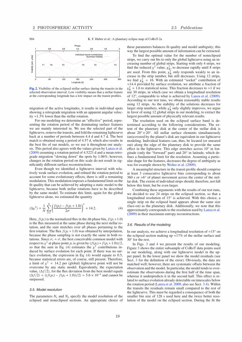
904 K. F. Huber et al.: A planetary eclipse map of CoRoT-2a
0 60 120 180 240 300 360
01/62/61/24/65/61
Vis
ibili
ty [
arb
. u
nits]
Longitude [d]
Phase
T1 T2T3 T4T5T6
Individual transit contributionsSummed Visibility
Fig. 2. Visibility of the eclipsed stellar surface during the transits in theselected observation interval. Low visibility means that a stellar featureat the corresponding longitude has a low impact on the transit profiles.
migration of the active longitudes, it results in individual spotsshowing a retrograde migration with an apparent angular veloc-ity ≈1.3% lower than the stellar rotation.
For our modeling we determine an “effective” period, repre-senting the rotation period of the dominating surface featureswe are mainly interested in. We use the selected part of thelightcurve, remove the transits, and fold the remaining lightcurveback at a number of periods between 4.4 d and 4.7 d. The bestmatch is obtained using a period of 4.57 d, which also results inthe best fits of our models, so we use it throughout our analy-sis. This period also agrees with the values given by Lanza et al.(2009) assuming a rotation period of 4.5221 d and a mean retro-grade migration “slowing down” the spots by 1.06%; however,changes in the rotation period on this scale do not result in sig-nificantly different surface reconstructions.
Even though we identified a lightcurve interval with rela-tively weak surface evolution, and refined the rotation period toaccount for some evolutionary effects, there is still a remainingmodulation. This modulation imposes a fundamental limit on thefit quality that can be achieved by adopting a static model to thelightcurve, because both stellar rotations have to be describedby the same model. To estimate this limit, again for the globallightcurve alone, we estimated the quantity
〈∆χ2〉 = 1
N
N∑
i=1
(f (pi) − f (pi + 1.0)
2σ
)2≈ 14.2. (4)
Here, f (pi) is the normalized flux in the ith phase bin, f (pi+1.0)is the flux measured at the same phase during the next stellar ro-tation, and the sum stretches over all phases pertaining to thefirst rotation. The flux f (pi + 1.0) was obtained by interpolation,because the phase sampling is not exactly the same in both ro-tations. Since σi ≈ σ, the best conceivable common model withrespect to χ2 at phase point pi is given by ( f (pi)+ f (pi+1.0))/2,so that the sum in Eq. (4) estimates the χ2 contributions in-duced by surface evolution for each point. If there was no sur-face evolution, the expression in Eq. (4) would equate to 0.5,because statistical errors are, of course, still present. Therefore,a limit of χ2 ≈ 14.2 per (global) lightcurve point will not beovercome by any static model. Equivalently, the expectationvalue, 〈∆ f /2〉, for the flux deviation from the best model equals〈∆ f /2〉 = 〈( f (pi) − f (pi + 1.0))/2〉 = 5.6 × 10⁻⁴ and cannot besurpassed.
3.5. Model resolution
The parameters Ne and Nn specify the model resolution of theeclipsed and noneclipsed sections. An appropriate choice of
these parameters balances fit quality and model ambiguity; thisway the largest possible amount of information can be extracted.
To find the optimal value for the number of noneclipsedstrips, we carry out fits to only the global lightcurve using an in-creasing number of global strips. Starting with only 4 strips, wefind the reduced χ2 value, χ2
R, to decrease rapidly until 8 strips
are used. From this point, χ2R
only responds weakly to an in-crease in the strip number, but still decreases. Using 12 strips,we find χ2
R= 16. With an estimated “socket” contribution of
≈14.4 provided by surface evolution, we attribute a fraction ofχ2
R≈ 1.6 to statistical noise. This fraction decreases to ≈1 if we
use 30 strips, in which case we obtain a longitudinal resolutionof 12°, comparable to what is achieved by Lanza et al. (2009).According to our test runs, we obtain reasonably stable resultsusing 12 strips. As the stability of the solutions decreases forlarger strip numbers, while χ2
Ronly slightly improves, we argue
in favor of using 12 global strips in our modeling, to extract thelargest possible amount of physically relevant results.
The resolution used on the eclipsed surface band is de-termined according to the following considerations. The ex-tent of the planetary disk at the center of the stellar disk isabout 20°× 20°. All stellar surface elements simultaneously(un)covered by the planet’s disk are equivalent in our lightcurvemodeling. Individual features can, thus, be located (or smearedout) along the edge of the planetary disk to provide the sameeffect in the lightcurve. This edge stretches across 10° in lon-gitude (only the “forward” part) and 20° in latitude, which de-fines a fundamental limit for the resolution. Assuming a partic-ular shape for the features, decreases the degree of ambiguity aswas for example shown by Wolter et al. (2009).
A meaningful structure in the transit profile should compriseat least 3 consecutive lightcurve bins corresponding to about360 s or ≈6° of planet movement across the center of the stel-lar disk. The extent of individual strips should, therefore, not fallbelow this limit, but be even larger.
Combining these arguments with the results of our test runs,we decided to use 24 strips on the eclipsed section, so that alongitudinal resolution of 15° is achieved. With this choice, asingle strip on the eclipsed band appears about the same size(face-on) as the planetary disk. Additionally, we note that thisapproximately corresponds to the resolution used by Lanza et al.(2009) in their maximum entropy reconstructions.
3.6. Results of the modeling
In our analysis, we achieve a longitudinal resolution of ≈15° onthe eclipsed section making up ≈17% of the stellar surface and30° for the rest.
In Figs. 3 and 4 we present the results of our modeling.Figure 3 shows the entire subsample of CoRoT data points usedin our modeling, along with our lightcurve model in the up-per panel. In the lower panel we show the model residuals (seeSect. 3 for the definition of the error). Obviously, the data arematched well; however, there are systematic offsets between theobservation and the model. In particular, the model tends to over-estimate the observations during the first half of the time span,whereas it underpredicts it in the second half. This effect is re-lated to surface evolution already detectable on timescales belowthe rotation period (Lanza et al. 2009, also see Sect. 3.4). Withinthe transits the residuals remain small compared to the rest ofthe lightcurve. This must be regarded a consequence of both thesmaller bin size of 128 s used here and the twice better reso-lution of the model on the eclipsed section. During the fit the
2 PHOTOSPHERIC ACTIVITY 2.5 Publications
19

K. F. Huber et al.: A planetary eclipse map of CoRoT-2a 905
0.9
0.91
0.92
0.93
0.94
0.95
0.96
0.97
0.9854248 54252 54254
Re
lative
brig
htn
ess
MJD [d]
T1 T2 T3 T4 T5 T6
-10
0
10
2 2.5 3 3.5 4
Re
sid
ua
ls [
σ]
Phase
Fig. 3. Upper panel: CoRoT data for rotational phases 1.85 to 3.85(2016 s binning for the global lightcurve and 128 s for the transits, redsymbols) and our model lightcurve (dashed blue curve). Lower panel:residuals of our model.
transit residuals are “overweighted” by a factor of ten to avoidthem to be prevailed by the much larger global residuals.Although, the deviations can be as large as 10σ, the mean de-viation of the global lightcurve from the model amounts to620 × 10−6 not far from the theoretical limit of 560 × 10−6 (cf.Sect. 3.4).
The lightcurve presented in Fig. 3 contains six transits (la-beled “T1 − 6”). The associated transit lightcurves are shown indetail with our models in Fig. 4. Each individual panel showsthe same transit twice: the lower curve represents a transit recon-struction from the full data sample (phases 1.85−3.85), and theupper curve denotes a reconstruction from only the first (T1−3)or second (T4−6) half of the sample data (shifted up by 0.03).The dotted lines show the transits as we would observe themwithout any activity on the eclipsed section of the surface, wherewe assume a brightness of 1 for the underlying photosphere.
The transit reconstructions obtained from half of the sam-ple data reproduce the transit substructure very accurately. Theresulting surface reconstructions are, however, unreliable wherethe surface is insufficiently covered (cf. Fig. 2, around longitudesof 180° and 320°). Interestingly, those reconstructions based ondata from two rotation phases also recover most of the transitsubstructure and are by no means off the mark. When both rota-tion periods are used, χ2 typically increases by 10−20%, a dif-ference hardly visible in Fig. 4. As an exception, the fit qualityof the third transit (T3) decreases dramatically, with χ2 increas-ing by a factor of ≈2.5. This is, however, mainly a consequenceof the observed surface evolution shifting the continuum level.The overall stability of the fit quality indicates that lifetimes ofsurface features are a few stellar rotations, which agrees with theresults of Lanza et al. (2009).
In Fig. 5 (lower and middle panels) we present the stripbrightness distribution pertaining to the lightcurve model shownin Figs. 3 and 4, i.e., a 1D-reconstruction of the surface. Weestimated mean and errors by recording the distribution of theparameter values obtained from 50 reconstructions with ran-domized starting points, and the respective distributions are in-dicated by the color gradients in Fig. 5. The error bars corre-spond to the associated standard deviations. They reflect the abil-ity of the fitting algorithm to converge to a unique extremum,which is determined by both the characteristics of the algorithmand the structure of the fit statistics. Investigating the brightness
0.92
0.94
0.96
0.98
1
1.9 1.91 1.92
Re
lative
brig
htn
ess
Phase
T1
2.28 2.29 2.3Phase
T2
0.92
0.94
0.96
0.98
1
2.66 2.67 2.68R
ela
tive
brig
htn
ess
Phase
T3
3.04 3.05 3.06Phase
T4
0.92
0.94
0.96
0.98
1
3.42 3.43 3.44
Re
lative
brig
htn
ess
Phase
T5
3.81 3.82Phase
T6
Fig. 4. Close-up of the six individual transits (128 s binning).Observations are drawn as red points (including 1σ errors). The up-per curve (black) in each panel shows the fit obtained from 1 rotation(phases 1.85 to 2.85 for T 1−3 and 2.85 to 3.85 for T 4−6); the lowercurve (blue) gives the fit obtained by modeling both rotations (as seenin Fig. 3). The dashed lines show the undisturbed transit profile forcomparison.
distribution of the noneclipsed strips, we notice a slight degen-eracy in some of the 12 noneclipsed strips; i.e., a fraction of thebrightness may be redistributed without considerable loss of fitquality. The averaging of the 50 reconstructions flattens out suchfeatures, thus acting like a regularization of the brightness distri-bution. No such effect is observed for the eclipsed strips.
We compared our results to the reconstructions given byLanza et al. (2009, their Fig. 4) and find our longitude scale tobe shifted by ≈70° with respect to the Lanza et al. scale. Our re-constructions show the same bright band at a longitude of ≈260°(330° in our work). Tentatively averaging over an appropriate“time band” in their Fig. 4, we also find qualitative agreementfor the remaining spot distribution.
Clearly, the flux fraction contributed by the eclipsed stripsis less than that of the noneclipsed strips, because the area theycover is smaller by a factor of five. In the upper panel of Fig. 5we show the lightcurve model contributions provided by theeclipsed and the noneclipsed section with their sum making upthe model for the CoRoT data, which is also shown. The medianflux level was subtracted from all curves to emphasize the mod-ulation amplitude in favor of flux level. Obviously, the modula-tion amplitudes induced by the eclipsed and noneclipsed sectionbalance approximately. This indicates that their influence on thestellar variability is about the same despite their large differencein size.
2.5 Publications 2 PHOTOSPHERIC ACTIVITY
20

906 K. F. Huber et al.: A planetary eclipse map of CoRoT-2a
Noneclipsed section
Eclipsed section
0 60 120 180 240 300 360
Longitude [degrees]
0.6
0.8
1
Re
lative
str
ip b
rig
htn
ess
Noneclipsed section
Eclipsed section
0.9
1
-0.02
-0.01
0
0.01
0.02
0.03
2 2.2 2.4 2.6 2.8 3
∆ f
lux
Phase
Noneclipsed section
Eclipsed section
Variability induced by eclipsed sectionVariability induced by noneclipsed section
Fig. 5. Upper panel: the CoRoT data (red symbols) and the flux mod-ulation contributed in our model by the eclipsed (blue curve) andnoneclipsed section (dotted gray curve) individually. All curves aremedian-subtracted. Middle and lower panels: Brightness distribution ofthe strips located on the eclipsed and noneclipsed sections of the sur-face. The color gradient renders the distribution obtained from 50 re-constructions with randomized starting points.
A visualization of our best-fit surface reconstruction is pre-sented in Fig. 6, showing a Hammer projection of the associateddistribution of surface brightnesses. The planet-defined low-latitude band shows especially dark features, e.g. in the rangeof 200° to 300° in longitude, and is clearly visible. Also thenoneclipsed sections of the star show significant variations. Notethat our map only shows the average brightness of these regions;since the noneclipsed regions are larger by area, they contributemore flux; however, the “missing” flux in these regions is likelyto also be concentrated in spots. In the following section we ad-dress the issue of the flux contribution from the eclipsed andnoneclipsed sections.
3.6.1. Brightness distribution and spot coverage
Without a very precise absolute flux calibration (as e.g. in Jefferset al. 2006), lightcurve analyses can usually only investigate theinhomogeneous part of the entire spot coverage. This statementis, however, partially invalidated by a transiting planet becauseit breaks the symmetry of the problem. Spots eclipsed by theplanetary disk distort the transit profiles regardless of whetherthey belong to a structure that appears symmetric on a globalscale or not.
As an example, assume that half the eclipsed section ofCoRoT-2a, say longitudes 0−180°, is spotted, while the otherhalf is covered by an undisturbed photosphere. Clearly, the tran-sits will be shallower when the planet eclipses the dark portionof the star, and they will be deeper when the bright section iseclipsed. Also, the lightcurve will be distorted. Assume as wellthat a comparable section between longitudes 180−360° is darkon the opposite hemisphere of the star outside the eclipsed band.In this case the global spot configuration is perfectly symmet-ric with respect to longitude and the global lightcurve does notshow any trace of activity. Nevertheless, the transits will still be
Fig. 6. Surface map of CoRoT-2a showing the reconstructed brightnessdistribution. Spots located on the noneclipsed surface are blurred overthe entire reconstruction strip because of their unknown latitude result-ing in the lower contrast compared to the eclipsed section.
0.8
1
0 60 120 180 240 300 360
Becl./B
non-e
cl.
Longitude [d]
0.94
Mean ratio
Fig. 7. Ratio of the surface brightness in the eclipsed (Becl.) andnoneclipsed (Bnon−ecl.) sections.
shallower when the planet eclipses the dark band, and they willstill be deeper when the bright surface is eclipsed.
If the spots were distributed symmetrically across the stel-lar surface, we would expect the stellar surface to be homoge-neously bright. In Fig. 7 we show the brightness ratio of eclipsedand noneclipsed sections as a function of longitude. Since thereare more eclipsed than noneclipsed strips, we always comparestrips covering the same longitude. Only in two cases is theeclipsed section brighter than its noneclipsed counterpart, whilein 22 cases it is not.
The mean ratio is 0.94 ± 0.01 so that the part of the starpassingly covered by the planet is found to be 6% darker thanthe rest of the surface. The remaining (nontransited) surface isbrighter on average, but locally it may even be darker.
4. Discussion and conclusions
We present a surface reconstruction for the planet host starCoRoT-2a. Our modeling is based on a CoRoT data interval cov-ering two full stellar rotations, and it treats the entire lightcurve –including the planetary transits – in a consistent way.
We show that a consistent modeling of the lightcurve ispossible using a static model, i.e., not including any spot evo-lution. Although surface evolution on scales of the stellar ro-tation period is seen in both the reconstruction of the globallightcurve (as already reported by Lanza et al. 2009) and thetransit lightcurves, this effect is weak in the context of our anal-ysis. The static model provides reasonable fits to six consecutivetransit lightcurves. The associated surface configuration changeslittle during this period, so the surface evolution must be rela-tively slow compared to the timescale of ≈9 d under considera-tion. This timescale is also valid for the lifetimes of spots on theeclipsed surface section.
Our results indicate that the planet-eclipsed band on the stel-lar surface is – on average – about 6% darker than the remainingpart of the surface. Lanza et al. (2009) note that the strength
2 PHOTOSPHERIC ACTIVITY 2.5 Publications
21

K. F. Huber et al.: A planetary eclipse map of CoRoT-2a 907
of differential rotation derived from their lightcurve fits seemsmuch lower than the expected values derived from measure-ments in other systems (Barnes et al. 2005). They speculate thatthis may indicate a spot distribution limited to a narrow latitudeband. If this is true, the latitude band is possibly located at lowlatitudes, i.e., within ±30° around the equator as observed on theSun. In this case it covers the eclipsed section where we find adarker surface, i.e., higher spot coverage. We caution that thisresult may also be influenced by the adopted planetary param-eters (mainly the size), which are hard to determine accurately(Czesla et al. 2009).
We checked whether the effect of gravitational darkeningcould significantly contribute to a darker surface in the vicinityof the equator. For the stellar parameters of CoRoT-2a, we findthat the (effective) gravitational accelerations at the poles andat the equator are equal to within 0.07%, so that gravitationaldarkening does not significantly contribute to the brightness gra-dient found in our modeling. This result is nearly independent ofthe assumed coefficient, β1 (T 4
eff gβ1 with the effective surface
temperature Teff and the surface gravity g), which is approxi-mately 0.3−0.4 for CoRoT-2a (Claret 2000).
The “narrow-band hypothesis”, i.e., a higher spot coveragein the planet-eclipsed section compared to the noneclipsed sur-face, also provides a natural explanation for the fact that both theeclipsed and noneclipsed surface regions account for about thesame amplitude of variation in the lightcurve. Using the Sun asan analogy again, we would qualitatively expect the same struc-ture, as seen under the planet path, on the opposite hemisphereas well: two “active belts” that are symmetric with respect tothe equator. The noneclipsed activity belt, which would be onlyobservable in the global lightcurve, would then be primarily re-sponsible for the variability of the lightcurve contributed by thenoneclipsed surface section.
We conclude that our results support a surface model con-sisting of active regions north and south of the equator, possi-bly even bands of spots at low latitudes analogous to the Sun.Further investigations of this system using more sophisticatedmodels (first of all surface evolution) and using the entire obser-vation interval of approximately 140 days have the potential ofrevealing more information on the constantly changing surfacedistribution of spots on CoRoT-2a.
Acknowledgements. K.H. is a member of the DFG Graduiertenkolleg 1351Extrasolar Planets and their Host Stars. S.C. and U.W. acknowledge DLRsupport (50OR0105).
References
Alonso, R., Auvergne, M., Baglin, A., et al. 2008, A&A, 482, L21Alonso, R., Guillot, T., Mazeh, T., et al. 2009, A&A, 501, L23Auvergne, M., Bodin, P., Boisnard, L., et al. 2009, A&A, 506, 411Barnes, J. R., Cameron, A. C., Donati, J.-F., et al. 2005, MNRAS, 357, L1Bouchy, F., Queloz, D., Deleuil, M., et al. 2008, A&A, 482, L25Claret, A. 2000, A&A, 359, 289Czesla, S., Huber, K. F., Wolter, U., Schröter, S., & Schmitt, J. H. M. M. 2009,
A&A, acceptedJeffers, S. V., Barnes, J. R., Cameron, A. C., & Donati, J.-F. 2006, MNRAS, 366,
667Lanza, A. F., Pagano, I., Leto, G., et al. 2009, A&A, 493, 193Press, W. H., Teukolsky, S. A., Vetterling, W. T., & Flannery, B. P. 1992,
Numerical recipes in C. The art of scientific computing, ed. W. H. Press, S. A.Teukolsky, W. T. Vetterling, & B. P. Flannery (Cambridge University Press)
Skrutskie, M. F., Cutri, R. M., Stiening, R., et al. 2006, AJ, 131, 1163Vogt, S. S., & Penrod, G. D. 1983, PASP, 95, 565Wolter, U., Schmitt, J. H. M. M., Huber, K. F., et al. 2009, A&A, 504,
561
2.5 Publications 2 PHOTOSPHERIC ACTIVITY
22

A&A 514, A39 (2010)DOI: 10.1051/0004-6361/200913914© ESO 2010
Astronomy&
Astrophysics
Planetary eclipse mapping of CoRoT-2a
Evolution, differential rotation, and spot migration
K. F. Huber, S. Czesla, U. Wolter, and J. H. M. M. Schmitt
Hamburger Sternwarte, Universität Hamburg, Gojenbergsweg 112, 21029 Hamburg, Germany
Received 18 December 2009 / Accepted 17 February 2010
ABSTRACT
The lightcurve of CoRoT-2 shows substantial rotational modulation and deformations of the planet’s transit profiles caused bystarspots. We consistently model the entire lightcurve, including both rotational modulation and transits, stretching over approxi-mately 30 stellar rotations and 79 transits. The spot distribution and its evolution on the noneclipsed and eclipsed surface sections arepresented and analyzed, making use of the high resolution achievable under the transit path.We measure the average surface brightness on the eclipsed section to be (5 ± 1)% lower than on the noneclipsed section. Adopting asolar spot contrast, the spot coverage on the entire surface reaches up to 19% and a maximum of almost 40% on the eclipsed section.Features under the transit path, i.e. close to the equator, rotate with a period close to 4.55 days. Significantly higher rotation periodsare found for features on the noneclipsed section indicating a differential rotation of ∆Ω > 0.1. Spotted and unspotted regions in bothsurface sections concentrate on preferred longitudes separated by roughly 180°.
Key words. planetary systems – techniques: photometric – stars: activity – starspots – stars: individual: CoRoT-2a
1. Introduction
The space-based CoRoT mission (e.g. Auvergne et al. 2009),launched in late 2006, provides stellar photometry of unprece-dented quality. One of CoRoT’s primary tasks is the search forextra-solar planets using the transit method. So far several sys-tems with eclipsing exoplanets were found, one of them CoRoT-2 harboring a giant close-in “hot-jupiter”.
The planet CoRoT-2b was discovered by Alonso et al.(2008), who determined the system parameters from transitsand follow-up radial velocity (RV) measurements. Bouchy et al.(2008) observed the Rossiter-McLaughlin effect using addi-tional RV measurements and determined the projected angleλ = (7.2 ± 4.5)° between the stellar spin and the planetaryorbital axis. Lanza et al. (2009) used the strong rotationalmodulation of the lightcurve to study the spot distributionand its evolution; they detect a stellar rotation period ofProt = (4.522 ± 0.024) d and two active longitudes on oppo-site hemispheres. The secondary eclipse of the planet was firstdetected by Alonso et al. (2009) in white light. Later the analy-sis was refined and extended by Snellen et al. (2010), detectingsignificant thermal emission of the planet; Gillon et al. (2009)repeated this work using additional infrared data. They also findan offset of the secondary transit timing indicating a noncircularorbit.
The determination of the planetary parameters by Alonsoet al. (2008) did not account for effects of stellar activity, whichis in general not negligible for active stars. Czesla et al. (2009)re-analyze the transits and derive new parameters for the planetradius Rp/Rs and the orbital inclination i considering the defor-mation of transit profiles due to spot occultation. This is espe-cially important for attempts to reconstruct active surface regionsfrom transit profiles. An analysis of a single transit by Wolteret al. (2009) shows the potential of eclipse-mapping and yieldedconstraints on the properties of the detected starspot. Similar
approaches to analyze signatures of starspots in transit profileswere also carried out by Pont et al. (2007) (HD 189733) andRabus et al. (2009) (TrES-1) primarily using data obtained withthe Hubble Space Telescope. In a more comprehensive approach,Huber et al. (2009) reconstructed an interval of the CoRoT-2lightcurve over two stellar rotations including the transits.
This work is based on the paper of Huber et al. (2009). Wenow analyze the entire data set of CoRoT-2, modeling both therotational modulation of the global lightcurve and transits simul-taneously. In this way we derive stellar surface maps for both thenoneclipsed and the eclipsed section of the star.
2. Observations and data reduction
The data were obtained in the first long run of the CoRoT satel-lite (May 16 to Oct. 15, 2007). The planetary system CoRoT-2(Star CorotID 0101206560) consists of an active solar-like G7Vstar and a large planetary companion on a close orbit. Due to itsedge-on view and an orbit period of only about 1.7 days, thislightcurve contains about 80 transits, roughly 3 during each stel-lar rotation.
The large surface inhomogeneities of this very active starare clearly visible in the rotational modulation of the CoRoTlightcurve taken over approximately 140 days. Although thereis surface evolution even on timescales of one stellar rotation,these changes are small compared to the modulation amplitude.Significant deformations of the transit profiles due to spots arealso visible throughout the whole time series.
The stellar and planetary parameters used throughout thisanalysis are given in Table 1. The extensive raw data analysisand reduction follows the descriptions in Czesla et al. (2009)and Huber et al. (2009).
In this paper we only analyze the alarm mode dataof CoRoT-2, when the satellite switched from a sampling
Article published by EDP Sciences Page 1 of 10
2 PHOTOSPHERIC ACTIVITY 2.5 Publications
23

A&A 514, A39 (2010)
Table 1. Stellar/planetary parameters of CoRoT-2a/b.
Stara Value ± Error Ref.
Ps (4.522 ± 0.024) d L09
Spectral type G7V B08
Planetb Value ± Error Ref.
Pp (1.7429964 ± 0.0000017) d A08
Tc [BJD] (2 454 237.53562 ± 0.00014) d A08
i (87.7 ± 0.2)° C09
Rp/Rs (0.172 ± 0.001) C09
a/Rs (6.70 ± 0.03) A08
ua, ub (0.41 ± 0.03), (0.06 ± 0.03) A08
References. taken from Lanza et al. (2009) [L09], Alonso et al. (2008)[A08], Bouchy et al. (2008) [B08], or Czesla et al. (2009) [C09].
Notes. (a) Ps - stellar rotation period; (b) Pp – orbital period, Tc – centraltime of first transit, i – orbital inclination, Rp,Rs – planetary and stellarradii, a – semi major axis of planetary orbit, ua, ub – linear and quadraticlimb darkening coefficients.
rate of 1/512 s−1 to 1/32 s−1 (which started after 3 tran-sits), and use the combination of the three color channels(“white” light). Our analysis starts after one stellar rotation atJD= Tc + Ps = 2454242.05562 (see Table 1) or a stellar ro-tation phase of φs = 1.0, respectively. We use units of stellarrotation phase in our analysis, the last point of our data intervalcorresponds to φs = 31.24. This leaves us with an observationspan of more than 30 stellar rotations containing 79 transits. Inthe following the first transit inside our data interval is labeled 0,the last 78.
3. Analysis
3.1. The model
The projected axes of the planetary orbit and the stellar rotationare co-aligned (Bouchy et al. 2008), which strongly suggests a3-dimensional alignment. Hence, the rotation axis of CoRoT-2ais inclined by approximately 88°. While this impedes the recon-struction of latitudinal information of surface features, the exis-tence of a planet crossing the stellar disk allows to access latitu-dinal information on spots beneath its path. During a planetarypassage the surface brightness distribution is mapped onto thelightcurve as deformations of the transit profiles. As a conse-quence of the co-aligned orientation of the planetary orbit andthe stellar spin, the surface band scanned by the planetary diskremains the same: the planet constantly crosses the latitudinalband between 6° and 26°. Accordingly, the stellar surface canbe subdivided into two sections: the eclipsed section and thenoneclipsed section (cf., Huber et al. 2009).
Our surface model subdivides the two individual sectionsinto a number of “strips”; Ne is the number of strips in theeclipsed and Nn in the noneclipsed section, respectively. Eachstrip represents a longitudinal interval inside the latitudinalboundaries of the corresponding section. The layout of our sur-face model is shown in Fig. 1 of Huber et al. (2009).
3.1.1. Model resolution and error estimation
The problem of lightcurve inversion is well known to be ill-posed, so that the parameter space is usually further constraintby a regularization. One such regularization is the maximum
Fig. 1. Observations and best fit model for CoRoT-2. The transit num-bers are plotted below the lightcurve; for a detailed presentation of thetransits see Fig. 9. See Sect. 3.4 for discussion.
entropy approach, applied, for example, by Lanza et al. (2009)in their analysis of CoRoT-2a.
We use a Nelder-Mead (NM) Simplex algorithm for mini-mization (Press et al. 1992). Our model does not require any
Page 2 of 10
2.5 Publications 2 PHOTOSPHERIC ACTIVITY
24

K. F. Huber et al.: Planetary eclipse mapping of CoRoT-2a
regularization because of its relatively small number ofparameters. As discussed by Huber et al. (2009), we choose anumber of strips balancing the improvement in χ2 and the dete-rioration in uniqueness. For higher strip numbers, adjacent stripsincreasingly influence each other because brightness can be re-distributed without significant loss of fit quality. In our erroranalysis we assume that there is a unique best-fit solution to ourproblem and that the NM algorithm approaches it to within thelimits of its ability to converge. Starting from the yet unknownbest-fit solution, brightness can be redistributed among the stripsat the expense of fit quality. A set of Nelder-Mead fit runs will,therefore, provide a sequence of solutions with different realiza-tions of this brightness redistribution.
We calculate 50 reconstructions with randomized startingpoints and adopt the average of all reconstructions as our mostappropriate model. As an estimate for the error of the stripbrightness, we use the standard deviation of the parameter val-ues, obtained from the set of reconstructions.
We do point out that the averaged solution appears smootherthan most individual reconstructions in the sense that the differ-ence between adjacent strip brightnesses is smaller. This can beunderstood in the picture of brightness redistribution, becausethe brightening of one strip may preferably be compensated bydarkening an adjacent one, which increases their contrast. Thiseffect is largely canceled out by the averaging, which makes itappear much like a regularization of the solutions.
It may be criticized that the brightness error we use is largelydetermined by the ability of the NM algorithm to converge to aunique solution. We emphasize, however, that the χ2 range cov-ered by the 50 reconstructions exceeds that required for ‘classi-cal’ error analysis, and the estimate will, therefore, remain ratherconservative from that point of view.
Our test runs indicate that for our purpose the most appro-priate number of strips to choose for the noneclipsed section isNn = 12, which will be used in our analysis. Larger numbers ofNn appear to already oversample the surface significantly. Thestrip number for the eclipsed section is chosen to be Ne = 24which approximately reflects the size of features that are resolv-able inside of transits (Huber et al. 2009).
3.2. Normalization
The observations are normalized with respect to the ab initio un-known spot-free photospheric flux of the star, which is definedas maximum brightness bphot = 1. Unfortunately, it is not trivialto obtain this photospheric flux level because spots are likely tobe located on the visible disk at all times.
A possible solution for this problem is to adopt the maxi-mum observed flux as photospheric. However, this presumablyintroduces an error because the brightest part of the lightcurveshows only the flux level of the stellar disk during the minimumobserved spot coverage, which needs not be zero. Lanza et al.(2009) determine an average minimum of flux deficit of approx-imately 2.5%. Tests with slightly varying maximum brightnessvalues in our reconstructions show no qualitative difference inthe brightness distribution except for a change in the average to-tal spot coverage; however, they show a significant decrease inχ2 of the lightcurve reconstructions for a maximum brightness1% to 2% larger than the highest observed flux. As a result wechoose a photospheric flux level of 2% higher than the maximumobserved flux. The entire lightcurve is normalized with respectto this value.
3.3. Lightcurve modeling
For analysis, the lightcurve is split into equally sized intervals,each covering one stellar rotation and three transits. Due to sur-face evolution detectable on timescales smaller than one stellarrotation, we choose to define a new interval after each transit.Thus, the resulting intervals overlap. Interval 0 contains the tran-sits number 0 to 2, interval 1 contains the transits number 1 to3, and so on. This way we end up with 76 lightcurve intervalswhich are individually reconstructed by our modeling algorithm.
Using fit intervals smaller than one stellar rotation could fur-ther reduce the influence of surface evolution. However, we needat least three transits in each interval to sufficiently cover theeclipsed section. Therefore, we always use a complete rotationfor each reconstruction interval.
We use the fitting method presented in Huber et al. (2009).Each fit interval is rebinned to 94 × 32 = 3 008 seconds for theglobal lightcurve and to 128 seconds inside of transits. Transitpoints are weighted with a factor of 10 higher than global pointsto give them approximately the same weight in the minimizationprocess. We assume the planet to be a dark sphere without anyemission; this seems to be a good approximation consideringa secondary transit depth of about (0.006 ± 0.002)% (Alonsoet al. 2009). All other necessary parameters can be found inTable 1.
We introduce a penalty function to suppress reconstructedbrightnesses above the photospheric value of one. Without thisboundary the brightness of individual strips exceeds this limit insome reconstructions. Strips with values above unity must be in-terpreted as regions with a brightness greater than the (defined)photosphere; however, in this approach we want to consider onlycool surface features, which was found to be a good approxima-tion by Lanza et al. (2009). Several tests showed that this penaltyfunction does not significantly alter the outcome of our recon-structions; it primarily prevents the minimization process fromgetting stuck in (local) minima outside the relevant parameterrange.
To analyze the transits accurately, we require an “undis-turbed transit profile”, which means a profile corrected for theeffects of stellar activity. This “standard transit profile” wasdetermined by Czesla et al. (2009), where a planet size ofRp/Rs = 0.172 was found. With the planetary parameters derivedby Alonso et al. (2008) no satisfactory fits to the transits andglobal lightcurve can be produced.
3.4. Results of the modeling
We present our lightcurve reconstruction in Fig. 1. It showsthe observed CoRoT-2 lightcurve (red triangles), including thetransits, and our reconstruction (blue solid line). The shown re-constructed lightcurve is a combination of all models for the76 fit intervals; their overlaps were combined using a Gaussianweighting. Each transit is labeled with its number on the loweredge of the graph; a more detailed picture of their fits is given inFig. 9, where we present all transits in a stacked plot.
Below the lightcurve the residuals σ = (O − C)/σO (O-observed lightcurve, C-reconstructed lightcurve,σO-error of ob-servation) are given. The mean values for σO are 1.8× 10⁻⁴ out-side and 6.9 × 10⁻⁴ inside of transits. Maximum values of theresiduals are approximately 10σ, which corresponds to a de-viation of about 0.2% between the observed and reconstructedlightcurves. On average, the absolute values of residuals are1.12σ or O −C = 4.4 × 10⁻⁴, respectively.
Page 3 of 10
2 PHOTOSPHERIC ACTIVITY 2.5 Publications
25

A&A 514, A39 (2010)
0
0.1
0.2
0.3
-5 -3 -1 1 3 5
Fra
ctio
n o
f p
oin
ts
Residuals [σ]
µt = +0.024
σt = 1.161
µg = -0.059
σg = 1.742
χ2red = 2.18
Fig. 2. Distribution of residuals σ between the observations and thebest fit model (see Fig. 1). The overall distribution is the sum of twoGaussians, one coming from inside the transits (mean µt and width σt)and the other coming from outside of them (global, mean µg andwidth σg). For details see Sect. 3.4.
Figure 2 shows the distribution of residuals from Fig. 1. Itis approximately Gaussian, although the underlying distributionis twofold: one component is a Gaussian distribution of residu-als from inside the transits with σt = 1.161, and another broadercomponent is coming from the residuals of the global lightcurve,which is significantly wider with σg = 1.742. The addition ofboth Gaussians reproduces the overall distribution of residualsaccurately. We calculate χ2
red= 2.18 from all residuals of the
entire lightcurve.The interpretation of χ2
redas an actual goodness-of-fit indi-
cator is not straightforward in this case. An increase of the stripnumber should lead towards χ2
redvalues of 1. Test calculations
show that our fit quality cannot be substantially improved be-yond a certain level when the number of strips is increased. Thislevel of χ2
redprimarily reflects the evolution of the lightcurve
within one stellar rotation, which cannot be improved withinour static model, and which is especially visible in the globallightcurve (σg ≫ σt). Unfortunately, it is very hard to quantifythis effect.
3.5. Construction of brightness maps
In Fig. 3 we present maps of the temporal evolution of the bright-ness distributions. The left panel gives the brightness map forthe noneclipsed, the right panel for the eclipsed surface section.The rows show the reconstructed brightness distributions for all76 lightcurve intervals; each interval is labeled by the number ofthe first transit it contains. Due to the different resolutions in thetwo surface sections, we linearly interpolate the brightness val-ues in each individual row; there is no interpolation applied be-tween different rows. To generate the combined brightness mapshown in Fig. 8 (left panel), the maps of the two separated sec-tions are weighted, corresponding to their disk fraction of 0.79for the noneclipsed and 0.21 for the eclipsed section, and added.The errors are combined the same way. Adjacent rows in ourmaps are not independent because the fit interval is only shiftedby one transit (≈1/3 stellar rotation) when moving from one rowto the next.
The errors are displayed directly below each map. For thebrightness values of the global lightcurve fit (Fig. 3, left panel),the mean error is about 1%, for the transits (Fig. 3, right panel) it
is approximately 3%. The errors in the latter map are larger (onaverage) and more inhomogeneously distributed because theyalso reflect the coverage of the eclipsed section by the transits;areas only marginally visible in transits cannot be reconstructedwith high accuracy.
The stellar longitude scale of our maps runs backwards from360° to 0°. This is due to our retrograde definition of the stellarlongitude l compared to stellar phases φs; their relation is l =(φN − φs) · 360° (with an integer stellar rotation number φN =[φs] + 1).
The identification of significant structures in these maps de-serves some attention. The brightness information is color codedusing black color for the darkest structures and white for photo-spheric brightness. Considering the approximate mean error ofeach map, we indicate areas with a brightness significantly be-low unity with yellow color. Hence, not only black areas of thesemaps are spots but yellow structures represent a significant de-crease in brightness as well.
4. Discussion
In this section we discuss and interpret the spot distributions ofour brightness maps and their evolution. This involves quite afew different aspects, which are often difficult to disentangle, andon which we focus on individually in the following subsections.
4.1. Identifying physical processes and detection limits
Our brightness maps allow us to witness the evolution of thestellar surface and, to some degree, to discriminate betweenindividual processes causing changes of the spot distribution:Emergence/dissociation, differential rotation, or migration ofsurface features leave potentially distinguishable signatures.Unfortunately, the high diversity of CoRoT-2a’s surface and alimited resolution complicate the interpretation of these signa-tures.
On the eclipsed section the position of a feature is fairlywell known and it is likely to be physically coherent. On thenoneclipsed section it is not clear whether a feature is actually asingle connected active region or a superposition of two (or evenseveral) different regions.
Features on the eclipsed section provide a valuable referencepoint for the detection of differential rotation. Systematic lon-gitudinal movements of spots in the transit map do not indicatedifferential rotation but rather a difference to the input rotationperiod. However, a comparison of transit and global maps couldreveal different rotation periods on different surface sections.
Systematic longitudinal movements of structures in theglobal map do not necessarily indicate differential rotation ei-ther. A simultaneous decay and growth of two distinct activeregions at different longitudes might leave a signature similarto a single differentially rotating active region. Therefore, theprocesses of differential rotation and spot evolution are hard todiscern.
A very interesting scenario is the possibility to find spot mi-gration due to the planet. If a spot moves from the noneclipsedto the eclipsed section, its signature also moves from the globalto the transit brightness map. If present, such signatures are de-tectable in high quality brightness maps.
In the following discussion we attempt to attribute signaturesin the brightness maps to the specific processes discussed above.Depending on the number of longitudinal strips used, map struc-tures have an estimated error in longitude of about half the strip
Page 4 of 10
2.5 Publications 2 PHOTOSPHERIC ACTIVITY
26

K. F. Huber et al.: Planetary eclipse mapping of CoRoT-2a
GLOBAL MAP TRANSIT MAP
Fig. 3. Left panel: brightness map reconstructed from the global lightcurve (noneclipsed surface). Right panel: brightness map for the recon-structions of the transits (eclipsed surface). The combination of both maps is presented in Fig. 8. Each row presents the reconstructed brightnessdistribution of one fit interval; the transit number indicates the number of this interval’s first transit. Each step in transit number equals a temporalstep of 1.74 days. The brightness is color-coded, the maximum photospheric brightness is unity. The error maps at the bottom of each panel showthe estimated reconstruction error. See Sects. 3.3 and 3.5 for details.
width, which is about ±7.5° for the transit and ±15° for theglobal map, respectively.
4.2. Spot coverage
The brightness maps of Fig. 3 show clear evidence of (a) a cover-age of a large fraction of the surface with dark features and (b) asubstantial evolution of this spot distribution within the roughly140 days of observations. Considering the pronounced rota-tional modulation of the lightcurve, and the persistently chang-ing shape between individual rotations, this result is hardly sur-prising. The lowest flux of the rotationally-modulated lightcurveis about 0.92 (modulo the uncertainty in lightcurve normaliza-tion, see Sect. 3.2); if the starspots were absolutely dark, theywould still cover 8% of the disk. The largest peak-to-peak vari-ation during one rotation spans from 0.98 to 0.92 indicatingroughly 6% more spots on the darker hemisphere.
Using a spot contrast of cs = 0.7, which is about the aver-age bolometric contrast of sunspots (Beck & Chapman 1993;Chapman et al. 1994), we determine a maximum spot coverageof 37% on the eclipsed and 16% on the noneclipsed section. Forthe entire stellar surface a maximum and minimum spot cover-age of 19% and 16% are derived.
Details on brightness values and spot coverage can befound in Fig. 4. The average brightness B is the mean bright-ness of each reconstruction interval. The top panel givesthe ratio between the mean brightness of the eclipsed andnoneclipsed sections, the second and third panel (from top)the eclipsed and noneclipsed brightnesses separately, and thebottom panel shows the variation of the total brightnessBTotal = (1 − A) · Becl. + A · Bnon−ecl. with A = 0.79. The associ-ated spot coverage fraction is calculated using (1 − B)/(1 − cs).
Instead of converting brightness into spot coverage, we canalso reverse the process. Assuming the darkest element of thetransit map is entirely covered by one spot, the reconstructedbrightness represents the spot contrast. One strip on the eclipsedsection has a size of about 1% of the entire surface. We obtain avalue of 0.76 for the darkest surface element of the transit map,which is not far from the solar spot contrast of 0.7. The minimumbrightness of 0.76 can be translated into a temperature contrast
0.920
0.940
0.960
0.980 4240 4260 4280 4300 4320 4340 4360 4380
Bec
l/B
no
n-e
cl
Julian date
0.880
0.900
0.92030
35
40
Bec
l
Sp
ot
co
ver
age
ecl
. [%
]
0.950
0.960
0.970 10
12
14
16
Bn
on
-ecl
Sp
ot
cover
age
no
n-e
cl.
[%]
0.940
0.945
0.950
0.955
0 5 10 15 20 25 30
16
18
20
BT
ota
l
Sp
ot
cover
age
all
[%
]Rotation phase
Fig. 4. Average brightness values of the eclipsed (Becl.) and noneclipsed(Bnon−ecl.) sections for each reconstruction interval. The y-axes on theright show the corresponding spot coverage for a spot contrast of 0.7.Top panel: ratio Becl./Bnon−ecl. of the mean brightnesses. Second panel
from top: mean brightness and spot coverage for the eclipsed sec-tion. Third panel from top: mean brightness and spot coverage for thenoneclipsed section. Bottom panel: total brightness BTotal; the blackcurve shows the results of Lanza et al. (2009) shifted by +9% (seeSect. 4.2).
of ∼400 K between the spot and the photosphere, which is atTp = 5625 K (Bouchy et al. 2008).
4.3. Rotation period
For CoRoT-2a Lanza et al. (2009) determine a rotation periodof (4.52 ± 0.14) d by means of the Lomb-Scargle periodogram,which the authors later refine to be Ps = (4.522 ± 0.024) daysby minimizing the longitudinal migration of their active longi-tudes. We adopted Ps for our reconstructions. It is almost identi-cal to the largest peak in the Lomb-Scargle periodogram (Fig. 5)
Page 5 of 10
2 PHOTOSPHERIC ACTIVITY 2.5 Publications
27

A&A 514, A39 (2010)
0
2000
4000
6000
8000
4 4.25 4.5 4.75 5 5.25 5.5
Po
wer
Period [days]
P1 P2P3
Fig. 5. Section of the Lomb-Scargle periodogram of the CoRoT-2lightcurve containing the highest peak. The three peaks are labeled P1 =4.53, P2 = 4.95, and P3 = 4.72 days according to decreasing power. Theadopted rotation period of our reconstructions, Ps = 4.522 days (Lanzaet al. 2009), is close to P1.
centered at P1 = 4.53 d. P1 is accompanied by two other distin-guishable peaks at P2 = 4.95 d and P3 = 4.72 d, which are re-lated to structures in our surface maps as discussed in Sect. 4.4.
Since the planet crosses the stellar disk in a latitudinal bandbetween 6° and 26°, spots on the eclipsed section must be lo-cated close to the equator. The approximate vertical alignmentof the darkest features in the transit map indicates that low-latitude features rotate close to the adopted rotation period of4.522 days used in our reconstructions. In contrast, features onthe noneclipsed section do show longitudinal migration, whichmay be attributed to differential rotation of spot groups at lati-tudes >∼30°. This finding suggests that active regions close to theequator dominate the modulation of the lightcurve.
A closer inspection of the transit map shows a small but con-stant longitudinal shift of about 60° over the entire 30 rotations.It is not only visible in the dark structures located at ∼200° and∼60° longitude, but for the bright region at ∼300° as well. Asa consequence, these low-latitude features do not rotate exactlywith a rotation period of 4.522 days but about 2° per rotationmore slowly, which translates into a rotation period of approxi-mately 4.55 days. Lanza et al. (2009) state a retrograde migrationof their second active longitude corresponding to this rotationperiod.
We recalculated the surface reconstructions adopting a rota-tion period of 4.55 days. As expected the longitudinal shift previ-ously detected in the transit map disappeared, but some featuresnow seem to migrate in the other direction. Therefore, the exactrotation period of features on the eclipsed section is probablyslightly smaller than 4.55 days. The global map changes accord-ingly when using a rotation period of 4.55 days; the brightnessdistribution reconstructed at larger transit numbers is shifted to-wards larger longitudes, but remains qualitatively the same, sothat these maps are not presented separately.
4.4. Longitudinal movement / differential rotation
Some attributes of the global map suggest a longitudinal move-ment of surface structures; a labeling of particularly interestingregions is given in Fig. 6. Especially considering the inactive re-gions, the bright structure B1 at the bottom left appears to movefrom ∼300° to ∼100° (B2) within about 4 stellar rotations. Itcontinues moving in the direction of decreasing longitude reach-ing roughly 240° near transit number 50 (B3). Regions B4 andB5 do not seem to fit well into the line drawn by B1, B2, and B3.However, a line connecting B4 and B5 roughly matches with thepreviously detected rotation period between 4.8 and 5.0 days.The tilted shape of the dark structure D1 roughly agrees with
Fig. 6. The global surface map (left panel of Fig. 3) with pronounceddark and bright features marked and labeled D1 – D3 and B1 – B5, re-spectively. The dash-dotted line and the arrows indicate the tentativemovement of bright regions (see Sect. 4.4).
this range of periods as well. D2 indicates a smaller rotation pe-riod consistent with P3.
Although such surface map characteristics do not necessar-ily prove differential rotation, they are certainly suggestive ofdifferential rotation. Assuming now this to be correct, we willelaborate on its consequences. The largest rotation periods weobtain from structures of the global map lie between about 4.8and 5.0 days. We studied the longitudinal movements of thesestructures on surface maps obtained from lightcurve reconstruc-tions applying different rotation periods and always end up withsimilar results. An examination of CoRoT-2’s periodogram re-veals a splitting up of the highest peak into three components:P1 = 4.53 d, P2 = 4.95 d, and P3 = 4.72 d (see Fig. 5). It is strik-ing that P2 is close to the rotation period determined from tiltedstructures in our global map.
If these rotation periods do arise from differential rotation,we can estimate a lower limit of its strength. The rotation pe-riod of eclipsed spots close to the equator is consistent with thehighest peak P1 = 4.53 days of the periodogram, the largest peri-ods detected in the global map are around P2 = 4.95 days; there-fore, we adopt this period for the most slowly rotating active re-gions. This way we determine a lower limit of ∆Ω > 0.1 rad/d orα > 0.08. This is consistent with values expected for stars withtemperatures and rotation periods similar to that of CoRoT-2(Barnes et al. 2005). Using a 3-spot model approach, Fröhlichet al. (2009) derive an estimate of ∆Ω > 0.11 rad/d, which is ingood agreement with our result.
Although the peaks in the periodogram fit nicely in with ourbrightness maps, attributing them to three active regions withassociated rotation periods may not be fully adequate. We sim-ulated several lightcurves with differentially rotating spots andexamined their periodograms. Although the main peak splits upinto different components, the periodogram does not necessar-ily map the exact rotation periods of the differentially rotatingspots to the peak barycenters. An exhaustive analysis of the pe-riodogram is beyond this work’s scope, but the above approachmay serve as an approximation, and it shows that the character-istics of the periodogram can be aligned with surface map at-tributes.
As an alternative, or maybe extension, to the interpretation interms of differential rotation, an evolution of the global activitypattern should be considered, which does not invoke longitudi-nal movement of individual surface features, but a redistribu-tion of strength between active regions. The spot distributionon the global map suggests sudden longitudinal relocations of
Page 6 of 10
2.5 Publications 2 PHOTOSPHERIC ACTIVITY
28

K. F. Huber et al.: Planetary eclipse mapping of CoRoT-2a
the most active feature. For the first ∼25 transits the dominantspotted region D1 keeps its position at ∼30° showing an ap-parent movement towards smaller longitudes at the end of thisinterval. Afterwards the dominant active region is found approx-imately 180° apart from the previous position in region D2. Such180°-jumps, or rather “hemisphere-jumps”, as the value of 180°should not be taken too seriously here, are found for inactive(bright) regions as well.
An appealing explanation for this apparent shift is a changeof the relative strength of two active regions, which does notinvolve movement of any of the structures themselves. Thesejumps are possibly a sign for some flip-flop scenario as al-ready claimed for other stars (Jetsu et al. 1993; Korhonen et al.2001), where the relative strength between two active longi-tudes is changing suddenly and periodically. The timescale ofthese “jump periods” derived from our global brightness mapis roughly 10 stellar rotations; however, this is not seen in thetransit map.
4.5. Lifetimes of features
Both the global and the transit map provide the possibility tomeasure lifetimes of spotted regions. For the noneclipsed sec-tion it is not clear whether a dark structure actually is a singleconnected active region or a superposition of several individualones at roughly the same longitude but completely different lati-tudes.
The transit map shows a high stability of the spot positions.One group of spots is located between 200° and 240°, which isstable up to transit number 35; then the spot coverage seems todecrease for about one stellar rotation. Afterwards the spot dis-tribution becomes more complicated and spreads over a largerarea. The left part of this more complex region, at about 210°longitude, is probably a continuation of the preceding active re-gion; however, at about 160° longitude a new, clearly separatedgroup of spots appears. This latter structure appears to have alifetime of approximately 10 stellar rotations, which would be ingood agreement with timescales observed on the global map.
Another group of spots is located between 0° and 100°. Atthe beginning of the observation these spots are spread over thislarger interval of about 100° on the eclipsed section; later, ap-proximately after transit number ∼50, they seem to concentratein a smaller interval. This active region seems to have a signif-icant fine structure in time, which might indicate smaller life-times of individual spot groups; however, those structures couldalso be artifacts of the reconstruction algorithm. We prefer theinterpretation that this active region, and the left side of the otheractive region, are persistent over all 30 rotations, although theyprobably contain smaller spots undergoing significant evolutionon much shorter timescales.
The left side of both maps (around 300° in longitude) showsbright regions which are least covered by spots during all obser-vations, indicating a lifetime of half a year for this “inactive lon-gitude”. For the darkest structures of the global map, maximumlifetimes of about 10 to 15 stellar rotations can be estimated.This is in agreement with the results of Lanza et al. (2009), whodetermine a lifetime of ≈55 days (=12 stellar rotations) for ac-tive regions, and identify this time span with the “beat period”visible in the lightcurve.
Although there are some structures in the transit map thatsuggest smaller lifetimes than half a year for individual spotgroups, the lifetimes of features on the two different surface sec-tions seem to be different. A direct comparison of the globaland the transit map is shown in Fig. 7. The active regions on
Fig. 7. Direct comparison of the two brightness maps of Fig. 3. Theglobal map is drawn in color, structures of the transit map are shownwith contour lines. Upper panel: map of bright structures in the globalmap with bnon−ecl. > 0.95. The contour line delimits brightness valuesof the transit map above becl. = 0.94. Lower panel: map of dark struc-tures with bnon−ecl. < 0.95. Here the contour lines indicate a transit mapbrightness of becl. = 0.87.
the eclipsed section remain active all the time despite their pos-sibly significant fine structure. In contrast, active regions onthe noneclipsed section evolve faster showing more pronouncedchanges and a longitudinal movement compared to the spots onthe eclipsed section. The reason for the apparent lifetime differ-ence is not clear. Possibly the darkest structures represent onlya superposition of several spotted groups at about the same lati-tude. If these groups change their mutual longitudinal positions,or a fraction of the spot groups dissolves, the dark structuresin our maps would brighten. In this case the darkest structureswould only represent special configurations of the spot distribu-tion and their “lifetimes” in our maps would not be directly con-nected to the lifetimes of individual active regions on the surface.
The stable vertical alignment of features in our transit mapcannot be caused by a systematically incorrect transit profileused in our reconstructions. The transits do not always cover ex-actly the same part of the eclipsed section, which is also visiblein the error distribution of the transit map; dark structures indi-cate where the coverage is best, bright where it is worst. Thus, anerror introduced by the transit profile would be distributed overthe entire map.
4.6. Comparing global and transit maps: spot migration?
Finally, there is the possibility of detecting signatures of spotmigration – the movement of spots from the equator to the polesor vice-versa – in our brightness maps. Figure 7 presents thedirect comparison of the brightest structures (upper panel) andthe darkest structures (lower panel) of the global and the transitmap. Especially the dark structure D2 (see Fig. 6) in the middleof the lower panel’s map suggests that features on the eclipsed
Page 7 of 10
2 PHOTOSPHERIC ACTIVITY 2.5 Publications
29

A&A 514, A39 (2010)
(2009)
Fig. 8. Left panel: brightness distribution of the entire surface for all reconstructed intervals; it represents a combination of both the global and thetransit map. The error for each bin of the brightness map is shown below. Right panel: comparison of our brightness distribution (contours) to thereconstruction of Lanza et al. (2009), which are shown in color coding. See Sect. 4.7 for details.
and noneclipsed sections are related. For the first 30 transitsthere is a dark feature of the transit map at this longitude, thenit starts to disappear when D2 becomes darker. This reflects ascenario where a spot group moves from the eclipsed sectionto the noneclipsed. After transit number 40, D2 starts to disap-pear while other structures appear on the eclipsed section. If thisreally represents a case of spot migration, the spot group eithermoves back onto the eclipsed section, or it stays outside and newspots emerge under the transit path.
A similar observation can be made concerning the brightstructures in the upper panel of Fig. 7. The bright structures inthe transit map between 60° and 120° alternate with the brightregions B2 and B4. First there is a bright structure on the eclipsedmap below region B2, then there is a little bit of both betweenB2 and B4, and after region B4 a bright structure is emerging inthe transit map.
It is impossible to prove whether these signatures reallyrepresent spot migration; probably some of them are due toother processes, e.g. short-term evolution of spotted regions.Nevertheless, there is a similarity to what one would expectto see in brightness maps from surfaces showing spot migra-tion. A behavior supporting a shift of spots from the eclipsedto the noneclipsed sections (and vice-versa) can be observed inFig. 4 (second and third panel). It suggests a correlation betweenthe mean brightnesses of the two sections; when the averagebrightness of the eclipsed section decreases, it increases on thenoneclipsed part. However, this correlation does not necessarilyprove a steady motion between the two sections and might aswell indicate that vanishing spots just reappear somewhere else.
4.7. Comparison to previous results
Figure 8 (left panel) displays the combined brightness map de-rived from both the eclipsed (transit map) and noneclipsed sec-tions (global map) of Fig. 3: the single maps are multiplied bytheir corresponding surface fractions (0.21 for the eclipsed and0.79 for the noneclipsed) and added.
Lanza et al. (2009) present a map of the surface evolutionderived from a fit to the global lightcurve (their Fig. 4) not in-cluding the transits. In the right panel of Fig. 8 we present acomparison of their results to ours. Since we do not use fillingfactors, we translated their map into brightnesses using their spotcontrast of 0.665. We take the resulting map (color coding) and
superimpose it on our combined map from both the eclipsed andnoneclipsed sections (contours). In the left panel of Fig. 8 thesame contour lines are drawn to provide a better comparison.Lanza et al.’s and our results show good agreement, althougha perfect match in fine-structure is neither found nor expected.Dark and bright structures are located at very similar positionsand the shapes are consistent.
Adding up the brightness values of each reconstruction inter-val of the map in Fig. 8 (left panel), we can study the variationsof the mean total brightness BTotal of the star. This is presentedin Fig. 4 (bottom panel). With a maximum of BTotal = 0.951 anda minimum value of 0.942, the maximum difference betweenthe highest and lowest average total brightness is only about1%, which is much less than the maximum brightness differ-ences within the brightness maps. This implies that the star as awhole does not change its overall spot coverage as dramaticallyas it redistributes it; when spots disappear, other spots show up.The solid line in the panel gives the comparison to the results ofLanza et al. (2009). We translated their values to our spot con-trast of 0.7 and shifted it by a constant spot coverage of +9% tomatch our points. Our average spot coverage of 17.5% is roughlytwice as high. Although, a 9% shift seems to be enormous, about80% of it (+7%) can be attributed to a different normalization ofthe lightcurve and, thus, photosphere. While Lanza et al. (2009)define the maximum flux in the lightcurve as their photosphericlevel, our photosphere is 2% brighter (cf. Sect. 3.2), which has tobe compensated by spots. We attribute the remaining 2% to thedifferences in the adopted models. In particular, we use longi-tudinal strips and spots can only be distributed homogeneouslyacross a strips, while Lanza et al. (2009) localize the spots in200 bins on the surface.
Previously, we detected an average brightness under theeclipsed section (6 ± 1)% higher than on the noneclipsed sec-tion (Huber et al. 2009). This value is redetermined from thereconstruction of the entire lightcurve presented in this paper. Itdecreases to (5.4 ± 0.9)% (see top panel of Fig. 4).
4.8. Brightness maps and lightcurve modulation
It is striking that the rotational variations of the star are addition-ally modulated with a beat period about a factor 10 to 15 larger.During the maxima of this large-scale modulation (at about tran-sit numbers 15, 45, and at the end of the lightcurve), the minima
Page 8 of 10
2.5 Publications 2 PHOTOSPHERIC ACTIVITY
30

K. F. Huber et al.: Planetary eclipse mapping of CoRoT-2a
Fig. 9. Observation (blue triangles) and reconstruction (red solid line) of 79 transits from the CoRoT-2 lightcurve. The first transit of each columnis shifted to a continuum of zero, each subsequent transit is shifted by −0.025. The number of each transit is annotated inside the plot. See Fig. 1for the entire lightcurve.
of the stellar rotation are deep and regular, i.e., the lightcurvehas only one distinct minimum per rotation. During the minimaof this beat period (at about transit numbers 30 and 60), the ro-tational modulation is flatter and more complex; the minima aresplit up in two. The beat period maxima indicate the existence ofone large active region or longitude dominating the stellar sur-face. The minima indicate that two smaller active regions at sig-nificantly different longitudes imprint their signatures onto thelightcurve leaving double-peaked structures during one stellarrotation. This means dark regions are redistributed on timescalesof 10 to 15 stellar rotations from essentially one large feature toat least two smaller, longitudinally separated ones, and then backto a large one.
This is also observable in our brightness maps. Figure 8shows a change of the dominant surface feature from ∼60° to∼220° at about transit number 20. Earlier the lightcurve wasdominated by one large active longitude leading to one broadminimum during each rotation. During the transition phase, es-pecially around transit number 25, the lightcurve minima be-come double-peaked. After transit number 30 the activity center
of the active longitude at 220° moves to about 180° and, thus,closer to the other active longitude at about 60°, which has notentirely disappeared and starts to grow stronger again. Becausethe active longitudes are closer now, the minima grow deeper;additionally, the bright region at 300° becomes larger and themaxima rise.
Again there are double-peak structures between transit num-bers 55 and 60 for the same reasons. The decrease of the strongmaxima is primarily due to the temporary change of the brightlongitude at 300°. Interestingly, the amplitude and width of theminima become even larger at the end of the lightcurve, wherethe active longitudes first move closer together. In the end, thefeature at ∼20° becomes dominant spreading over almost 60° inlongitude and leading to very low lightcurve minima.
The main reason why the rotation period of the star is sonicely indicated by almost constantly separated maxima of thelightcurve – despite the pronounced surface evolution – is thatthe on average brightest part of the surface, located on the inac-tive longitude at 300°, remains stable at its position.
Page 9 of 10
2 PHOTOSPHERIC ACTIVITY 2.5 Publications
31

A&A 514, A39 (2010)
5. Conclusions
We present a reconstruction of the complete CoRoT-2 lightcurve– including transits – covering about 140 days or 30 stellar rota-tions. In contrast to previous work, both the transit profiles andthe rotationally-modulated global lightcurve are fitted simulta-neously leading to a consistent solution for the entire lightcurve.From the transits the brightness distribution on the eclipsed sur-face section is recovered, which is the part of the surface be-tween 6° and 26° latitude constantly eclipsed by the planet. Thenoneclipsed section is reconstructed from the rotational modula-tion.
The evolution of the spot distributions on both surface sec-tions is presented in two maps showing the surface brightnessdistribution as a function of time. The composite map, whichshows the evolution of the entire surface, is juxtapositioned withpreviously published results. The results are found to be in agree-ment taking into account different modeling approaches and as-sumptions.
The transit map shows two preferred longitudes densely cov-ered with spots and separated by approximately 180°. Both ac-tive regions persist for the entire observing time of ∼140 days,although they undergo significant evolution in size, structure,and brightness. In the transit map they show a constant retro-grade movement indicating that the adopted stellar rotation pe-riod of Ps = 4.522 days does not exactly describe their rotation.We determine that these low-latitude features rotate at a periodof approximately 4.55 days, which is also true for the long-livedinactive longitude at ∼300°.
The global map is more complex than the transit map pre-sumably because the structures it describes represent a super-position of features at similar longitudes but different latitudes.Usually it shows only one dominant dark feature at a time, whichchanges position after approximately 10 to 15 stellar rotations.Again these dominant features are separated by about 180° inlongitude. A persistent inactive longitude exists at about 300°similar to the one in the transit map and at about the same po-sition. The global map indicates that there are features locatedon the noneclipsed section with significantly larger rotation pe-riods than 4.522 days. This suggests the presence of differentialrotation with spots moving more slowly at high latitudes than atlow latitudes. We estimate a differential rotation of ∆Ω > 0.1 orα > 0.08, respectively.
Assuming a spot contrast of 0.7, the spot coverage of theeclipsed section reaches a maximum of 37%, which is morethan twice as large as the maximum on the noneclipsed sec-tion. On average the eclipsed section is (5 ± 1)% darker thanits noneclipsed counterpart. Sunspots are located within ±30°around the solar equator. Similarly, our results indicate that spotgroups on CoRoT-2 are also concentrated in a low-latitude “ac-tive belt”.
Acknowledgements. We thank A. F. Lanza for kindly providing us with theirresults for comparison. K.H. is a member of the DFG Graduiertenkolleg 1351Extrasolar Planets and their Host Stars and acknowledges its support. S.C. andU.W. acknowledge DLR support (50OR0105).
Note added in proof: Late in the review process, we becameaware of a paper by Silva (2003, ApJ, 585, L147) where plan-etary eclipse mapping is modeled using images of the Sun.Contemporaneously to our work, Silva-Valio et al. (2010, A&A,510, A25) used a very different approach to examine the transitsof the CoRoT-2 lightcurve for properties of starspots.
References
Alonso, R., Auvergne, M., Baglin, A., et al. 2008, A&A, 482, L21Alonso, R., Guillot, T., Mazeh, T., et al. 2009, A&A, 501, L23Auvergne, M., Bodin, P., Boisnard, L., et al. 2009, A&A, 506, 411Barnes, J. R., Cameron, A. C., Donati, J.-F., et al. 2005, MNRAS, 357, L1Beck, J. G., & Chapman, G. A. 1993, Sol. Phys., 146, 49Bouchy, F., Queloz, D., Deleuil, M., et al. 2008, A&A, 482, L25Chapman, G. A., Cookson, A. M., & Dobias, J. J. 1994, ApJ, 432, 403Czesla, S., Huber, K. F., Wolter, U., Schröter, S., & Schmitt, J. H. M. M. 2009,
A&A, 505, 1277Fröhlich, H., Küker, M., Hatzes, A. P., & Strassmeier, K. G. 2009, A&A, 506,
263Gillon, M., Lanotte, A. A., Barman, T., et al. 2010, A&A, 511, A3Huber, K. F., Czesla, S., Wolter, U., & Schmitt, J. H. M. M. 2009, A&A, 508,
901Jetsu, L., Pelt, J., & Tuominen, I. 1993, A&A, 278, 449Korhonen, H., Berdyugina, S. V., Strassmeier, K. G., & Tuominen, I. 2001,
A&A, 379, L30Lanza, A. F., Pagano, I., Leto, G., et al. 2009, A&A, 493, 193Pont, F., Gilliland, R. L., Moutou, C., et al. 2007, A&A, 476, 1347Press, W. H., Teukolsky, S. A., Vetterling, W. T., & Flannery, B. P. 1992,
Numerical recipes in C. The art of scientific computing, ed. W. H. Press, S. A.Teukolsky, W. T. Vetterling, & B. P. Flannery (Cambridge University Press)
Rabus, M., Alonso, R., Belmonte, J. A., et al. 2009, A&A, 494, 391Snellen, I. A. G., de Mooij, E. J. W., & Burrows, A. 2010, A&A, in pressWolter, U., Schmitt, J. H. M. M., Huber, K. F., et al. 2009, A&A, 504, 561
Page 10 of 10
2.5 Publications 2 PHOTOSPHERIC ACTIVITY
32

3 X-RAY ASTRONOMY 3.2 X-ray instrumentation
3 The X-ray perspectiveof magnetic activity inyoung stars and theirenvironments
In this section I outline the development of X-ray astronomy and describe the most importantcharacteristics of X-ray instrumentation. I givean overview of those aspects putting my workinto context, and, finally, present my own con-tributions.
3.1 A short history of X-ray as-tronomy
The dawn of X-ray astronomy came in thewake of a new technology; namely that ofrocketry. As the mean free path of X-rayphotons in air (at sea level) is of the order ofmeters, the Earth’s atmosphere must be leftbehind to observe an extraterrestrial source.The first X-ray observations were carried outusing rocket-borne instrumentation. Duringone of the flights, the first extrasolar X-raysource, Scorpius X-1, was discovered (Giacconiet al. 1962). Although subsequent rocketexperiments were carried out, the total X-rayexposure time available in 1970 was no morethan about one hour.
This changed dramatically after Decem-ber 12, 1970, when the first X-ray satellite,UHURU, was launched. UHURU carried outboth an all-sky survey and pointed observa-tions. It discovered 300 new X-ray sourcesand achieved an angular resolution of a fewarcminutes, which allowed to identify thesources with various kinds of celestial objects.Among the most notable results of the missionare the discovery of enormous amounts of hotgas in galaxy clusters, which in one fell swoopdoubled the mass of known baryonic matterin the local universe, and the realization thataccretion can serve as a highly efficient energysource (for a summary see, e.g., Giacconi2003).
The success of UHURU provided substan-tial momentum for the realization of successormissions, of which the first was Skylab, a
manned American space laboratory. It was,among others, equipped with instrumentsproviding the first spatially resolved X-rayimages of the Sun (e.g., Zombeck et al. 1978).The next extrasolar X-ray mission followedin 1978 when the EINSTEIN satellite waslaunched into orbit. Compared to UHURU,the EINSTEIN observatory provided en-hanced resolution, sensitivity, and, for the firsttime, allowed for spectroscopy in the X-rayregime. With EINSTEIN, the number of X-raysources and the detail in which they couldbe studied increased significantly. The dataprovided by EINSTEIN not only deepenedour understanding of the extragalactic sources,but also revealed X-ray emission associatedwith virtually all kinds of main sequence stars.About two decades after UHURU, the ROSATobservatory was launched to carry out the thenext, much more efficient survey of the X-raysky during which more than 100 000 sourceswere discovered. Besides the survey, manypointed observations were carried out untilthe mission ended in 1999. Although, moresensitive X-ray observatories are operatedtoday, the ROSAT data remain the mostrecent all-sky survey.
Today, important X-ray telescopes forextrasolar observations are Chandra, XMM-Newton, Suzaku, and Swift, of which Chandrais the most relevant for the work at hand.
3.2 X-ray instrumentation
A major challenge in observational high energyastronomy is focusing the radiation. In the X-ray regime conventional mirrors as used in op-tical telescopes proved to be inappropriate forcollecting light, so that an alternative approachwas needed. A possible solution was proposedby Wolter (1952), and it was named after him.
The basic physical concept behind the work-ing of a Wolter telescope is total reflection of X-ray photons after grazing incidence on metallicsurfaces. Because of the required grazing pho-ton incidence, the appearance of Wolter tele-scopes differs substantially from optical mir-rors. As an example, Fig. 6 shows the telescopebuild for the Chandra X-ray observatory, which
33
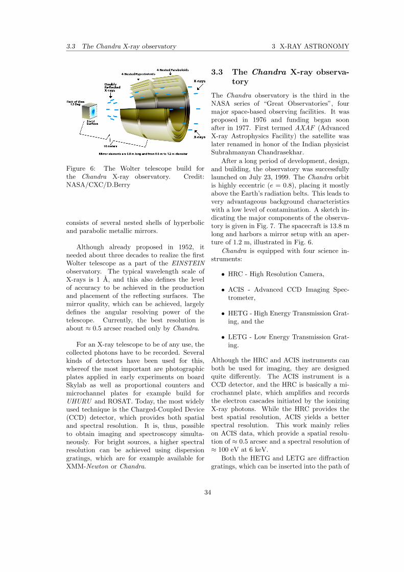
3.3 The Chandra X-ray observatory 3 X-RAY ASTRONOMY
Figure 6: The Wolter telescope build forthe Chandra X-ray observatory. Credit:NASA/CXC/D.Berry
consists of several nested shells of hyperbolicand parabolic metallic mirrors.
Although already proposed in 1952, itneeded about three decades to realize the firstWolter telescope as a part of the EINSTEINobservatory. The typical wavelength scale ofX-rays is 1 A, and this also defines the levelof accuracy to be achieved in the productionand placement of the reflecting surfaces. Themirror quality, which can be achieved, largelydefines the angular resolving power of thetelescope. Currently, the best resolution isabout ≈ 0.5 arcsec reached only by Chandra.
For an X-ray telescope to be of any use, thecollected photons have to be recorded. Severalkinds of detectors have been used for this,whereof the most important are photographicplates applied in early experiments on boardSkylab as well as proportional counters andmicrochannel plates for example build forUHURU and ROSAT. Today, the most widelyused technique is the Charged-Coupled Device(CCD) detector, which provides both spatialand spectral resolution. It is, thus, possibleto obtain imaging and spectroscopy simulta-neously. For bright sources, a higher spectralresolution can be achieved using dispersiongratings, which are for example available forXMM-Newton or Chandra.
3.3 The Chandra X-ray observa-tory
The Chandra observatory is the third in theNASA series of “Great Observatories”, fourmajor space-based observing facilities. It wasproposed in 1976 and funding began soonafter in 1977. First termed AXAF (AdvancedX-ray Astrophysics Facility) the satellite waslater renamed in honor of the Indian physicistSubrahmanyan Chandrasekhar.
After a long period of development, design,and building, the observatory was successfullylaunched on July 23, 1999. The Chandra orbitis highly eccentric (e = 0.8), placing it mostlyabove the Earth’s radiation belts. This leads tovery advantageous background characteristicswith a low level of contamination. A sketch in-dicating the major components of the observa-tory is given in Fig. 7. The spacecraft is 13.8 mlong and harbors a mirror setup with an aper-ture of 1.2 m, illustrated in Fig. 6.
Chandra is equipped with four science in-struments:
• HRC - High Resolution Camera,
• ACIS - Advanced CCD Imaging Spec-trometer,
• HETG - High Energy Transmission Grat-ing, and the
• LETG - Low Energy Transmission Grat-ing.
Although the HRC and ACIS instruments canboth be used for imaging, they are designedquite differently. The ACIS instrument is aCCD detector, and the HRC is basically a mi-crochannel plate, which amplifies and recordsthe electron cascades initiated by the ionizingX-ray photons. While the HRC provides thebest spatial resolution, ACIS yields a betterspectral resolution. This work mainly relieson ACIS data, which provide a spatial resolu-tion of ≈ 0.5 arcsec and a spectral resolution of≈ 100 eV at 6 keV.
Both the HETG and LETG are diffractiongratings, which can be inserted into the path of
34

3 X-RAY ASTRONOMY 3.4 Stars in X-rays
Figure 7: Major components of the Chandra X-ray observatory. Credit: NASA/CXC/NGST
light to obtain high resolution spectra of indi-vidual sources, which are recorded using ACIS.
Due to the great success of Chandra the ini-tial 5 year mission schedule has been extended,and Chandra has currently been in operationfor more than 10 years.
3.4 Stars in X-rays
The first direct detection of X-ray emissionfrom the solar corona was made during a rocketflight in 1949 (Burnight 1949). About twodecades later, Catura et al. (1975) reportedthe first discovery of X-ray emission from astellar system, Capella, and their result wassoon corroborated by Mewe et al. (1975), whowere the first to explain the observed X-rayemission with the presence of a corona.
With the exception of extraordinarily hotsources such as white dwarfs, coronal X-rayemission of stars does not interfere with photo-spheric contributions, as is the case for opticalor ultraviolet light. Therefore, X-ray emissionprovides an excellent means to study stellarcoronae and stellar activity. Fortunately, wefind a perfect example of a corona on our Sun,where it can be spatially resolved and studiedin great detail. Rosner et al. (1978) formulateda model of the quiet solar corona, in which themagnetic field was a main ingredient, and thecorona was made up of magnetic loops. Theauthors derived scaling laws for the coronalloops, which allowed to interpret the structure
Figure 8: X-ray sources across theHertzsprung-Russel diagram. Source sam-ple compiled from Berghoefer et al. (1996),Hunsch et al. (1998a), Hunsch et al. (1998b),and Hunsch et al. (1999).
in the coronae of other stars as scaled versionsof solar structures, without being able toactually resolve them.
Although stars have also been observedwith other X-ray observatories, the progressachieved by the EINSTEIN and, in particular,the ROSAT observatory were outstanding.Before EINSTEIN only the most extremestellar sources were known, but as EINSTEINwas observing the sky, stars all across theHertzsprung-Russel diagram showed up asX-ray sources (Vaiana et al. 1981), and sowere identified as a class of abundant X-rayemitters. The enhanced sensitivity of ROSATallowed to study stellar populations in muchmore detail, in particular, it was possible toanalyze volume limited samples of stars.
Schmitt et al. (1995) report an X-ray detec-tion rate of ≈ 90 % among M and K type starsin the solar neighborhood (7 pc), and as thestudy was extended (Schmitt 1997) the authorsfound similar detection rates for G and F typestars within 13 pc from the Sun. Yet, Schmitt(1997) failed to detect a single A type star ear-lier than A7 from their sample; an outcome,consistent with X-ray emission originating inmagnetically heated coronae, which should, in-deed, not be present in such stars, because they
35

3.5 How to study cool material in X-rays 3 X-RAY ASTRONOMY
posses no outer convection zones. It should benoted that early A stars may actually be intrin-sically X-ray bright in some cases, due to othermechanisms (Czesla & Schmitt 2007a, and ref-erences).
Massive B and O type stars were also foundto be X-ray bright (Berghoefer et al. 1996), andtheir emission is believed to originate in shocksdriven by their massive winds (e.g., Lucy &White 1980). Figure 8 shows the distributionof a ROSAT sample of X-ray sources in theHertzsprung-Russel diagram. Clearly, the mainsequence and the giant branch can be identified,and there is no type of star not showing up asan X-ray source.
Studies of activity indicators in the visualsuch as Ca II H&K (e.g., Baliunas et al. 1995)had already revealed that the stellar youthis a particularly active phase, a conclusionsoon confirmed by X-ray observations. Starforming regions arise from the collapse of alarge molecular cloud, in which dozens orthousands of stars are formed (see, e.g., McKee& Ostriker 2007, for an extensive review). Theevolution of the newly born stars is divided intofour categories, class 0-III. This classificationmainly describes steps in the stellar evolutionranging from deeply embedded cores still inthe process of collapse (class 0), over evolvedprotostars with envelopes and disks (class I),which evolve into pre main-sequence stars withdisks from which they still accrete significantamounts of matter (class II, classical T-Tauristars), and, finally, reach the weak-line T Tauristage (class III) when accretion has virtuallyceased.
It was EINSTEIN to discover the first X-rays from T Tauri stars. Feigelson & Decampli(1981) report the detection of X-ray emissionfrom 8 T Tauri stars in Taurus and Orion, ofwhich one, DG Tauri, was found to be highlyvariable; all were found to be quite X-raybright with X-ray luminosities in the range of1030−31 erg/s. The number of X-ray detectedyoung stellar objects (YSO) was greatly in-creased by ROSAT. Yet, star forming regionsare locations with a high source density, whichare often deeply embedded in circumstellarmaterial located in disks and envelopes as well
as in the remains of the cloud from which theyemanated. This combination interfered withboth the spatial resolution provided by theearly X-ray observatories and the relativelysoft bands (≤ 3 keV) which were covered.
The advent of XMM-Newton and Chan-dra revolutionized the study of star formingregions, because the available resolution andeffective area increased by about an orderof magnitude, and also the accessible bandwas extended mainly into the harder regime(≈ 0.2 − 10 keV). Using these observatories,several studies of star forming regions havebeen carried out; most notably the Taurusregion was extensively observed with XMM-Newton in the frame of the “XMM-Newtonextended survey of the Taurus molecularcloud” (Gudel et al. 2007) and Orion was tar-geted with Chandra. The observation of Orionis the deepest Chandra observation dedicatedto a single star forming region and was carriedout in the frame of the “Chandra Ultra-DeepProject” (COUP), which comprises about 1 Msof exposure time distributed over ≈ 13 days.COUP revealed 1616 X-ray sources in Orion(Getman et al. 2005b), and the sources werethen studied in many respects. For example,Getman et al. (2005a) investigated the Orionmembership of the sources, Feigelson et al.(2005) analyzed the X-ray properties of theOrion region, and Preibisch et al. (2005)focused their effort on the origin of X-rayemission in T Tauri stars, to name but a few5.
The space-based X-ray observatories havedemonstrated that virtually all stars are X-rayemitters, and the study of this emission has be-come a major tool in understanding the stellaractivity and evolution.
3.5 How to study cool material inX-rays
X-rays can only be produced in environments,which allow the transfer of sufficiently largeenergy portions to photons. Appropriateconditions can for example be found in plas-mas heated to millions of Kelvins or when
5see http://www.astro.psu.edu/coup/ for a morecomplete listing of related works.
36

3 X-RAY ASTRONOMY 3.5 How to study cool material in X-rays
Figure 9: Sketch of a fluorescent event. Credit:NASA/CXC/M.Weiss
particles are accelerated to relativistic ener-gies. Nonetheless, it is possible, under certainconditions, to study cold material in the X-rayregime.
Cold material can be studied by its effecton already produced X-rays. One possibility isto study the absorption characteristics of coldmaterial. For example absorption edges, i.e.,sudden changes in the absorption cross sectionoriginating in the structure of the atomic elec-tron shells, can be used to draw conclusions oncold material, which, of course, must be locatedin the line of sight to do so. This restriction canbe overcome by studying the radiation originat-ing from reprocessing of X-rays in cold mate-rial. One such reprocessing channel is fluores-cence.
The term “fluorescence” was coined byStokes (1852) and derives from the mineral“fluorite”. A sketch of a fluorescent processis given in Fig. 9. A photon of energy εi isabsorbed by an atom or ion (panel a) being leftin an excited state with an electron vacancyon an inner shell (panel b). The ion possiblyreleases its excess energy in form of a photonwith well defined energy, εo, i.e., a fluorescentphoton (panel c), and the result of many suchdeexcitations is a narrow emission line at thatenergy. As already noted by Stokes, the energyof the reemitted photon is generally lowerthan that of the absorbed one (εo < εi). Inthe process, any charged particle, for examplean electron, may take the role of the photonexciting the ion.
Fluorescent lines may in principle be ob-served from all elements contained in an illumi-nated cold plasma, yet, not all are of the same
Figure 10: Estimate for the strength of the flu-orescent Kα line of several elements.
importance in astrophysics today. The fluores-cent line gaining the most attention is that orig-inating in neutral or lowly ionized iron (hence-forth “Fe Kα I line”) for several reasons. Thereis a strong fourth power dependence of the flu-orescence yield, i.e., the probability for fluores-cent deexcitation, on atomic number, makingheavier elements stronger fluorescent sources,and iron is by an order of magnitude the mostabundant element heavier than Neon. Assum-ing similar cross sections for photoelectric ab-sorption, a rough estimate for the number offluorescent photons contributed by a specific el-ement, X, can be derived from
strength ∼ Z4 ×Ab(X) ×∫ ∞Ke
1
εeε/kT dε . (2)
Here, Z is the atomic number of the element,Ke is its K edge energy, and kT = 3 keV wasassumed. Figure 10 shows the estimate for allelements with atomic numbers between 18 and30, demonstrating the dominance of the ironcontribution.
The Fe Kα I line energy of ≈ 6.4 keV liesin a spectral region where the continuum con-tribution of typical thermal X-ray spectra withtemperatures of a few keV is small, the densityof other spectral features is low, and, finally,the energy band can be observed with today’sX-ray observatories.
The study of the Fe Kα I line has notonly become a major tool to analyze the
37

3.6 Publications 3 X-RAY ASTRONOMY
innermost portions of the engines operating inactive galactic nuclei, where the gravitationalattraction of the black hole dominates its envi-ronment, but is also a valuable instrument tostudy the less extreme environments of stars.In our Sun the Fe Kα I line has long beendetected and used to study the compositionof the solar photosphere. Promising sourcesbeyond the solar system are young stars, whichare still surrounded by the remains of the cloudthey emanated from. In the two followingpublications, fluorescent X-ray emission fromyoung stars in Orion is analyzed with a specialemphasis on its temporal evolution.
The major contribution to these workswas provided by myself, however, not withoutsupport and ideas provided by my supervisorJ.H.M.M. Schmitt.
38

A&A 470, L13–L16 (2007)DOI: 10.1051/0004-6361:20077741c© ESO 2007
Astronomy&
Astrophysics
Letter to the Editor
The nature of the fluorescent iron line in V 1486 OrionisS. Czesla and J. H. H. M. Schmitt
Hamburger Sternwarte, Universität Hamburg, Gojenbergsweg 112, 21029 Hamburg, Germanye-mail: [email protected]
Received 27 April 2007 / Accepted 24 May 2007
ABSTRACT
The fluorescent 6.4 keV iron line provides information on cool material in the vicinity of hard X-ray sources as well as on thecharacteristics of the X-ray sources themselves. First discovered in the X-ray spectra of the flaring Sun, X-ray binaries and activegalactic nuclei (AGN), the fluorescent line was also observed in a number of stellar X-ray sources. The young stellar object (YSO)V1486 Ori was observed in the framework of the Chandra Ultra Deep Project (COUP) as the source COUP 331. We investigate itsspectrum, with emphasis on the strength and time variability of the fluorescent iron Kα line, derive and analyze the light curve ofCOUP 331 and proceed with a time-resolved spectral analysis of the observation. The light curve of V 1486 Ori shows two majorflares, the first one lasting for ≈20 ks with a peak X-ray luminosity of 2.6 × 1032 erg/s (dereddened in the 1−10 keV band) and thesecond one – only partially observed – for >60 ks with an average X-ray luminosity of 2.4 × 1031 erg/s (dereddened). The spectrum ofthe first flare is very well described by an absorbed thermal model at high temperature, with a pronounced 6.7 keV iron line complex,but without any fluorescent Kα line. The X-ray spectrum of the second flare is characterized by even higher temperatures (>∼10 keV)without any detectable 6.7 keV Fe XXV feature, but with a very strong fluorescent iron Kα line appearing predominantly in the 20 ksrise phase of the flare. Preliminary model calculations indicate that photoionization is unlikely to account for the entire fluorescentemission during the rise phase.
Key words. stars: early-type – stars: activity – X-ray: stars
1. Introduction
The COUP data set provides a nearly continuous 13 day longX-ray observation of the Orion nebula star forming region andis currently one of the best suited data sets for the explorationof the X-ray properties of large and homogeneous samples ofyoung stars. Substantial analysis of this data set has alreadybeen performed (e.g. by Getman et al. 2005). In particular,Tsujimoto et al. (2005) carried out a systematic search for theoccurrence of the fluorescent iron Kα line at 6.4 keV, iden-tifying 7 COUP sources with detectable fluorescent emission.This emission line is particularly interesting since it can providea wealth of information on the emitting source(s). Fluorescent6.4 keV photons – hereafter referred to as Fe I Kα photons – re-sult from a de-excitation of neutral or lowly ionized iron atoms,following an excitation leaving the iron ion with a K-shell va-cancy. When the latter is filled by another (mostly L-shell) elec-tron, the excess energy can be carried by a fluorescent photon.Highly ionized iron can also show this behavior, but the transi-tion energy rises because of the reduced screening of the innerelectrons from the nuclear charge. Several processes lead to theejection of a K-shell electron and, thus, to the creation of theFe I Kα line. During the process of photoionization a K-shellelectron is ejected from iron after the absorption of a photon withan energy exceeding 7.11 keV. Alternatively, high energy parti-cles can eject K-shell electrons with the same threshold energy.
The first detection of the fluorescent Fe I Kα line wasreported in the context of solar physics (e.g. Neupert et al.1967). A model succeeding in explaining most of the so-lar Fe I Kα emission with photoionization only was proposed and
evaluated by Bai (1979), yet, e.g., Zarro et al. (1992) argue thatphotoionization alone is not sufficient to account for all of thesolar Fe I Kα emission. Fluorescent Kα line emission has alsobeen reported from other celestial X-ray sources. It is typicallyencountered in the high-energy emission from AGN and X-raybinaries, which are characterized by high X-ray luminosities andrather hard X-ray spectra, thus providing large photon numbersabove the 7.11 keV threshold for photoionization. Fabian et al.(1989) detect the fluorescent iron line in the spectrum of theX-ray binary Cyg-X1, and Tanaka et al. (1995) were the first toreport the relativistically broadened line in the spectrum of theAGN MCG-6-30-15. Recent observations with XMM-Newtonand Chandra extended the class of Fe I Kα line emitters toa number of stellar sources, such as the class I YSO Elias 2-29(Favata et al. 2005), the above seven COUP sources discussedby Tsujimoto et al. (2005), and the YSO YLW 16A for whichImanishi et al. (2001) carried out time-resolved spectroscopy.
In this letter we present a detailed analysis of the X-ray prop-erties of the YSO V 1486 Ori (=COUP 331) with emphasis onits Fe I Kα emission, which was already reported by Tsujimotoet al. (2005), who measured a normalization of 2.6(0.1−4.6) ×10−7 ph/(cm2 s) with an equivalent width of 126 eV for thefluorescent line. Unfortunately, the YSO V 1486 Ori has sofar not received much attention at other energy bands. Fromthe 2MASS-all-sky survey we infer its infrared magnitudes as12.5 mag, 10.6 mag, and 9.4 mag, in the J, H, and Ks bands,respectively. Tsujimoto et al. (2005) show that the infrared col-ors of V 1486 Ori do not match the regions of reddened dwarfsor giants and argue for the presence of a NIR-emitting innerdisk. Moreover a rotation period of (6.09 ± 0.3) d is known for
Article published by EDP Sciences and available at http://www.aanda.org or http://dx.doi.org/10.1051/0004-6361:20077741
3 X-RAY ASTRONOMY 3.6 Publications
39

L14 S. Czesla and J. H. H. M. Schmitt: The nature of the fluorescent iron line in V 1486 Orionis
Fig. 1. Background-subtracted light curve of COUP 331 with 2 ks bin-ning. Inserted panels show close-up views of the flares I and II.
V 1486 Ori (Herbst et al. 2002; Stassun et al. 1999). FollowingTsujimoto et al. (2005) we adopt a distance of 450 pc for Orion.
2. Observations and data analysis
The COUP data was obtained during 13 consecutive daysin Jan. 2003 with the Advanced CCD Imaging Spectrometer(ACIS) on board the Chandra X-ray observatory. The total ex-posure time is ≈840 ks, separated into 6 observation segmentsextending over a total time of ≈1140 ks. All observations havethe same aimpoint (α = 5h35m17s and δ = −523′40′′) and thefield of view covers an area of 17′ × 17′; the source COUP 331is located at α = 5h35m9.2s and δ = −530′58′′ (cf. Getmanet al. 2005). Our analysis is based on the pre-processed pho-ton data provided by the Chandra pipeline; for further analysiswe applied the CIAO-software in version 3.4. We first screenedthe photon data for events in the 0.3−13 keV energy band tosuppress background. Thereafter, we defined source and back-ground regions as a circle with an 8 arcsec radius and an annulusextending from ≈14–32 arcsec, both centered on the nominalsource position.
2.1. The light curve
We generated the background-subtracted 2−9 keV band lightcurve of COUP 331 shown in Fig. 1. The 6 observation seg-ments can be clearly identified. For most of the COUP observa-tions COUP 331 was recorded at a count rate of 3.3 × 10⁻³ cts/s,except for two periods. A strong flare (termed “flare I”) oc-curred ≈90 ks after the beginning of the observation. The flarerapidly rises to its peak within ≈4 ks, the decay is again quiterapid with an e-folding time of τdecay = 5.2 ks, but, unfortu-nately, is only partially observed. A second, less prominent butvery significant count rate enhancement (termed “flare II”) oc-curred 1080 ks after the start of the COUP campaign. This sec-ond flare was also not fully covered. Flare II has a much slowerrise phase lasting for ≈20 ks, and thereafter, the 2−9 keV bandcount rate remains more or less constant for at least 40 ks whenthe COUP observations were terminated. For the rest of the ob-servations COUP 331 was found in quiescence.
Fig. 2. Spectrum of COUP 331 during flare I (upper curve) and the qui-escent phase (lower curve), both fitted with an absorbed VAPEC model.
2.2. Spectral analysis
In the following section we carry out temporally resolved spec-tral analysis of the flare I, flare II, and quiescent phases ofCOUP 331; note that all quoted errors refer to 90% confidenceintervals unless stated otherwise. COUP 331 is located about7 arcmin off-axis, hence it does not appear as a perfectly sym-metric point-source. However, we regard its image distortion asweak and apply the CIAO standard tools for the extraction ofpoint-source spectra (i.e. psextract). The spectra were ana-lyzed using the XSPEC environment in version 11.3.1.
2.2.1. The quiescent phase
The quiescent phase spans the 0−1050 ks time interval with theexception of the first flare event, and is the longest lasting phase,covering ≈90% of the total observation time. Note that we disre-gard a ≈20 ks contribution preceding flare II. During quiescenceCOUP 331 is detected with a net count-rate of 3.3 × 10⁻³ cts/scorresponding to an (unabsorbed) X-ray luminosity of 1.6 ×1030 erg/s. We checked for temporal changes in the quiescentspectrum, but did not find evidence for any significant variations.The quiescent X-ray spectrum is well described by an absorbedthin-thermal plasma model (we used the VAPEC models) withall metal abundances – apart from Fe, which is left as a free pa-rameter – fixed to 0.3 times the solar values. In Fig. 2 we showthe data and the fit; the best fit model parameters are presented inTable 1, where we list the derived absorbing hydrogen column-density, the temperature, the iron abundance and the fit quality.
2.3. Flare I
For an analysis of flare I we considered all data recorded inthe time interval from 87.5 to 102 ks; the spectrum of flare I isshown in Fig. 2. The flare spectrum is very well described by thesame model as applied for the quiescent phase (cf. Sect. 2.2.1)with somewhat different spectral parameters listed in Table 1.We find – as expected for a flare – an enhanced temperature of6.8 keV, leading to a spectrum with a clearly detected Fe line fea-ture at 6.7 keV, but with no detected excess emission at 6.4 keV.From the spectrum we derive an (unabsorbed) peak X-ray lu-minosity of LX = 2.6 × 1032 erg/s (in the 1−10 keV band)reached directly after the rise phase, and – with an e-foldingtime of 5.2 ks for the decay phase – a total energy output of
3.6 Publications 3 X-RAY ASTRONOMY
40

S. Czesla and J. H. H. M. Schmitt: The nature of the fluorescent iron line in V 1486 Orionis L15
Table 1. Fit parameters for the absorbed VAPEC model.
Phase nH Temp. AbFe χ2/d.o.f.[1022 H/cm2] [keV] [Ab]
Quiescent 1.091.210.97 3.03.4
2.6 0.320.540.12 131.6/134
Flare I 1.281.411.18 6.88.2
5.5 0.731.020.46 94.2/99
Flare II 1.551.661.41
>∼13 ≈0.88a 102/95
a This value is ill-constrained since temperature-dependent.
∆E ≈ 1.4 × 1036 erg in the same band. With these numbers,flare I observed on COUP 331 is among the largest stellar flaresever observed.
2.4. Flare II
For the analysis of flare II we considered all data recorded after1080 ks (cf. Fig. 1). The X-ray spectrum was generated and an-alyzed in the same fashion as those of the quiescent and flare Iphases. From the spectrum of the entire observed flare II phase(see Fig. 3) we calculate an 1−10 keV band X-ray luminosityof 2.4 × 1031 erg/s. Considering a duration of at least 60 ks, thetotal energy output in this energy band is ∆E > 1.4 × 1036 erg.
In the fit process of the flare II data we encountered two prob-lems. First, the absence of temperature-sensitive features in thespectrum – especially the hot Fe XXV feature at 6.7 keV andits Fe XXVI counterpart near 7 keV – prevents us from tightlyconstraining the plasma temperature. We find that any choiceof the temperature beyond 10 keV leads to acceptable fits, andthus decided to apply a value of 13 keV. Second, the spec-trum shows definite excess emission above the thermal con-tinuum at 6.4 keV, which we attribute to the Fe I Kα line.We therefore included an additional instrumentally broadenedGaussian component centered at 6.4 keV into our model andrefitted, leaving only the normalization of the Gaussian com-ponent free to vary. The thus obtained fit is shown in Fig. 3,which shows the obvious presence of the 6.4 keV line and vir-tual absence of the 6.7 keV Fe XXV feature. The resulting fitparameters for the thermal model are again listed in Table 1,and for the Gaussian component we arrive at a normalizationof 5(3.3−6.7) × 10−6 ph/(cm2 s), corresponding to an equiva-lent width of 685(452–918) eV. As is obvious from Fig. 3, theinclusion of a Gaussian component at 6.4 keV into the modelsignificantly increases the fit quality.
As a first result we thus note that the 6.4 keV emission fea-ture is present – at best – only during 60 ks during flare II. Inorder to further temporally constrain the presence of the 6.4 keViron line we constructed a background-subtracted 6.1−6.7 keVnarrow-band light curve of COUP 331 with a 4 ks binning inaddition to the 2 ks binned 2−9 keV band light curve; both lightcurves are shown in Fig. 4. As is clear from Fig. 4 the 2−9 keVband light curve stays more or less constant after the rise topeak, while the 6.1−6.7 keV narrow-band light curve decaysquite rapidly. We therefore subdivided the the flare II phase datainto three consecutive 20 ks time intervals, denoted by “rise-phase”, “phase II”, and “phase III” as indicated in Fig. 4. TheX-ray spectra in the 5–8 keV region corresponding to these timeintervals are shown in Fig. 5. In these plots the solid line in-dicates the thermal model described earlier. For all spectra thesame model was applied, but we allowed the normalizationsof the VAPEC and Gaussian component to be fitted indepen-dently for all time intervals; all other parameters were regardedglobally. Figure 5 clearly demonstrates an evolution of the
Fig. 3. The COUP 331 spectrum during flare II with a close-up of the5−8 keV energy band. Two model fits are indicated. First, (solid line)an absorbed thermal model and second (dashed line), the same thermalmodel with additional instrumentally-broadened Gaussian componentcentered at 6.4 keV.
Fig. 4. The background-subtracted narrow-band light curve (solid line)of COUP 331 during the last 80 ks of the COUP observation. The lightcurve peaks in the rise-phase of flare II. For clarity the 2−9 keV lightcurve is also shown (dotted line – scaled to fit the plot range).
Fe I Kα line strength. Interestingly the line normalization de-creases as time proceeds, while the underlying thermal spectrumremains almost unaffected. We thus interpret the variations in thenarrow-band light curve shown in Fig. 4 as arising from varia-tions in the Fe I Kα feature’s strength. Note that the constancy ofthe thermal spectrum does not imply the same for the tempera-ture, since the latter exceeds 10 keV, producing a flat spectrumin the “low energy” band we are observing. The Kα feature isstrongest during the flare II rise phase where our fits yield a lineflux of 9.1(5.8−13.4)× 10−6 ph/(cm2 s) (an EW of ≈1400 eV)while in phase II and III it is reduced to 3.04(0.8–7.6) and0.9(0–4.8) × 10−6 ph/(cm2 s), respectively. This is also reflectedby the narrow-band light curve around 6.4 keV (cf. Fig. 4).
3. Interpretation and conclusions
Our time resolved analysis of the COUP X-ray data of theYSO COUP 331 shows that for ≈90% of the entire observationtime the object is found in a quiescent state characterized byan X-ray temperature of 30−40 MK. Two major flares are cov-ered by the COUP observation. In the first data segment a rel-atively short duration event with a peak X-ray luminosity of
3 X-RAY ASTRONOMY 3.6 Publications
41

L16 S. Czesla and J. H. H. M. Schmitt: The nature of the fluorescent iron line in V 1486 Orionis
Fig. 5. Time-resolved 5.5−8 keV section of the COUP 331 spectrum(cf. Fig. 4). Note the decrease of the Fe I Kα line’s strength.
2.6 × 1032 erg/s occurred, which clearly shows the 6.7 keV ironfeature, but no Fe I Kα emission.
In the last COUP data segment a long duration flare eventoccurred; starting with a ≈20 ks rise phase it lasted >60 ks. Thedecay of this flare cannot be constrained because the COUP ob-servations were stopped. The total amount of energy released inthe 1−10 keV energy band is >1.4 × 1036 erg; the X-ray temper-ature of this flare is extremely large (>∼10 keV) and can in fact notbe well constrained with the Chandra data. A clear and highlysignificant detection of the fluorescent Kα line is obtained onlyduring the 20 ks rise time of this flare; at later times the line maystill be present albeit at a lower level. This event on COUP 331resembles a huge flare observed on Algol, observed by Favata &Schmitt (1999) with BeppoSAX, which also shows a slow risephase, followed by a nearly constant phase – lasting for ≈80 ks –in its 1.6−10 keV band light curve. However, the corresponding15−100 keV band light curve clearly shows the characteristics ofa decay phase (cf., Favata & Schmitt 1999, Figs. 1 and 2). Theenergy output of 1.4 × 1037 erg derived by Favata & Schmitt(1999) in the 0.1−10 keV band compares well to the numbersestimated for COUP 331, note however that no Fe I Kα line wasdetected.
The precise temporal association between Fe I Kα lineemission and high energy continuum is necessary in order toquantitatively assess the origin of the Fe I Kα emission observed
in COUP 331; we find that the actual photon flux in the flu-orescent Kα line during the flare II rise phase is 35 timeslarger than reported by Tsujimoto et al. (2005). This discrep-ancy arises because Tsujimoto et al. (2005) give time-averagedvalues, whereas our values refer to several limited time inter-vals. The X-ray temperature during the flare event was extremelylarge; the total luminosity in the Fe I Kα line alone is ≈2.3 ×1030 erg/s. While these circumstances appear to favor the ex-citation of the Fe I Kα line through photoionization, prelimi-nary model calculations challenge such a scenario. We repeatedthe calculations carried out by Bai (1979) applying a reflectorwith cosmic abundances. We used the same branching ratios andcross sections for iron, but slightly different cross section for ab-sorption by other elements composed according to cosmic abun-dances. Furthermore, we located the source directly on the re-flector to make it subtend half the sky, thus providing an upperlimit for the fluorescent iron line flux. The illuminating inputspectrum was modeled as a thermal X-ray spectrum with a tem-perature of 13 keV, normalized to the measured fluxes. Our pre-liminary calculations show that an already optimally assumedfluorescence geometry significantly underpredicts the observedFe I Kα flux, making an interpretation of the Fe I Kα line throughphotoionization difficult to accept. However, these calculationswill be extensively discussed in a larger and systematic contextin a forthcoming paper, where we will also address its impact onthe characteristics of COUP 331 and other sources with fluores-cent Kα emission.
Acknowledgements. S.C. acknowledges support from the DLR undergrant 50OR0105.
ReferencesBai, T. 1979, Sol. Phys., 62, 113Fabian, A. C., Rees, M. J., Stella, L., & White, N. E. 1989, MNRAS, 238, 729Favata, F., & Schmitt, J. H. M. M. 1999, A&A, 350, 900Favata, F., Micela, G., Silva, B., Sciortino, S., & Tsujimoto, M. 2005, A&A, 433,
1047Getman, K. V., Flaccomio, E., Broos, P. S., et al. 2005, ApJS, 160, 319Herbst, W., Bailer-Jones, C. A. L., Mundt, R., Meisenheimer, K., &
Wackermann, R. 2002, A&A, 396, 513Imanishi, K., Koyama, K., & Tsuboi, Y. 2001, ApJ, 557, 747Neupert, W. M., Gates, W., Swartz, M., & Young, R. 1967, ApJ, 149, L79Stassun, K. G., Mathieu, R. D., Mazeh, T., & Vrba, F. J. 1999, AJ, 117, 2941Tanaka, Y., Nandra, K., Fabian, A. C., et al. 1995, Nature, 375, 659Tsujimoto, M., Feigelson, E. D., Grosso, N., et al. 2005, ApJS, 160, 503Zarro, D. M., Dennis, B. R., & Slater, G. L. 1992, ApJ, 391, 865
3.6 Publications 3 X-RAY ASTRONOMY
42
Astronomy & Astrophysicsmanuscript no. line˙light c© ESO 2010June 28, 2010
Puzzling fluorescent emission from OrionS. Czesla and J.H.M.M. Schmitt
Hamburger Sternwarte, Universitat Hamburg, Gojenbergsweg 112, 21029 Hamburg, Germany
Received 02.04.2010/ accepted 24.06.2010
ABSTRACT
Fluorescent X-ray emission offers one of the rare possibilities to study cool material in the X-ray regime. In the beginning used toanalyze the composition of the solar photosphere, the availability ofChandra and XMM-Newton has made the study of fluorescentemission a major tool for investigating cool material surrounding active,young stars and the inner parts of galactic nuclei. Yet, thequestion whether photoionization alone is the excitation mechanism of fluorescent X-ray emission or electron collisional excitationalso contributes is not completely settled. In this work, we develop a new technique to search for fluorescent emission and analyze itstemporal behavior, which we apply to a sample of 106 young, active stars in Orion. Our analysis yields a sample of 23 X-ray sourceswith fluorescent emission, including 6 objects already reported on in an earlier study. The fluorescent sources show a large variety intheir temporal behavior. While the fluorescent emission is associated with soft X-ray flares in some cases, it sometimes appears as aquasi persistent feature, or is seen during bona-fide quiescent periods. We conclude that fluorescent X-ray emission can be observedin a much larger fraction of young, active stars then previously believed. The temporal variability is often hard to reconcile with thephotoionization model, which remains, however, plausible if we allow for suitable geometries. It prevails over electron collisionalexcitation, mainly because the energetics of the latter are physically challenging.
Key words. Stars: activity; Stars: flare; X-rays: stars
1. Introduction
Fluorescent emission pushes the horizon of X-ray astronomybe-yond the observation of high energy material, carrying the im-print of cold matter into the X-ray regime. The origin of fluores-cent photons is cool, neutral matter pervaded by ionizing photonor particle radiation originating in a nearby high energy source.Following an inner shell ionization in the cold matter, excitedions potentially release their energy in form of fluorescentpho-tons, which convey information on the existence, structure, andcomposition of their creation site. Geometries appropriate forproducing a detectable amount of fluorescent emission are com-mon in a variety of celestial X-ray sources, and fluorescent X-ray emission has been reported in many targets including activegalactic nuclei and young stellar objects.
The interaction of an ion with high energy radiation can re-sult in the removal of one of the ion’s inner shell electrons.In thecontext of fluorescent emission, two conceivable mechanisms ofK-shell electron removal are at issue: Photoionization by soft X-rays and collisional excitation by electrons with kinetic energyin excess of the K-shell ionization edge. Independent of thein-teracting particle, an excited ion returns to a lower energystatethrough a rearrangement of its electron configuration, as a conse-quence of which the excess energy of the excited state is releasedby one of two competing processes. Either it is deposited in an“Auger electron”, being expelled from the ion, or it is released inthe form of a fluorescent photon. The probability of photon emis-sion rises strongly with increasing atomic number (Bambyneket al. 1972) and is termed the “fluorescence yield”. Consultingtypical solar system or cosmic abundance patterns (e.g., Anders& Grevesse 1989), iron becomes the most promising candidateto search for fluorescent emission. The K-shell ionization en-ergy of neutral iron is 7.112 keV, and the energy of its Kα linelies in the X-ray regime at about 6.4 keV; both numbers changeslowly with increasing ionization (e.g., Kaastra & Mewe 1993).
Spin-orbit interaction and the effects of photon scattering createa characteristic line profile (e.g., Sunyaev & Churazov 1996),which can, however, hardly be resolved with today’s instrumen-tation in astronomy.
Astronomical detections of the fluorescent Kα line of neu-tral or lowly ionized iron (in the following “Fe Kα I line”),were first obtained from solar observations (e.g., Neupert et al.1967; Doschek et al. 1971), in particular, during solar flares. Thequestion how much photoionization and collisional excitation byelectrons contributes to the observed solar fluorescent emission,was addressed by several authors. Parmar et al. (1984) analyzea sample of solar flares and conclude that ‘most, if not all,’ ofthe fluorescent X-rays are due to photoionization, and that theirresults agree well with associated simulations provided byBai(1979). Even though Zarro et al. (1992) and Emslie et al. (1986)do find evidence for a contribution of fluorescent photons causedby electron collisional excitation during the impulsive phase ofindividual flares, they also agree that the bulk of the fluorescentemission must be attributed to photoionization. The argument forphotoionization as the dominant process is based on the strengthor equivalent width of the fluorescent line as well as its temporalrelation to the observed hard and soft X-ray flux.
About thirty years after the reports of fluorescent emissioninsolar X-ray spectra, Tanaka et al. (1995) published their discov-ery of the Fe Kα I line in the spectrum of the active galactic nu-cleus (AGN) MGC-6-30-15. In excess of an imprint of cold ma-terial, this line also carries information on the relativistic space-time structure at its origin, providing a deep insight into the innerparts of an AGN. Ballantyne & Fabian (2003) argue that also inAGN sources photoionization largely dominates over electronor proton collisional excitation. The discovery of Tanaka et al.sparked an intensification of the search for the Fe Kα I line inX-ray sources, in the wake of which fluorescent emission wasalso discovered in several stellar sources other than the Sun.
1
3 X-RAY ASTRONOMY 3.6 Publications
43
S. Czesla and J.H.M.M. Schmitt: Puzzling fluorescent emission from Orion
Stellar sources with reported fluorescent emission includeYLWA 16 (Imanishi et al. 2001) with a Fe Kα I line detec-tion during a flare, HR 9024 for which Testa et al. (2008)present evidence for the Fe Kα I line in aChandra High EnergyTransmission Grating spectrum, and Elias 29, which shows a flu-orescent line of variable strength (Giardino et al. 2007). With theexception of HR 9024, the above stars are young stellar objects(YSOs). While photoionization remains the most common ex-planation for the origin of the fluorescent photons, Giardino et al.(2007) argue that the characteristics of the fluorescent emissionobserved from Elias 29 are hard to reconcile with the predictionsof the photoionization scenario and suggest a nonthermal elec-tron population invisible in soft X-rays as a possible explanationfor their findings.
As young stellar sources are known to possess large amountsof cold circumstellar material in the form of disks or envelopes,it seems reasonable to search for the Fe Kα I line in star formingregions. The Orion Nebula is a center of recent and still ongo-ing star formation, harboring a wealth of young stellar objects invarious evolutionary states. Orion was also the target of a longChandra observation known as the “Chandra Orion UltradeepProject” (COUP) (e.g, Getman et al. 2005). Tsujimoto et al.(2005) carried out a search for the Fe Kα I line in the COUPdata and presented a sample of seven COUP sources with a flu-orescent Fe Kα I line detection. One of their sources was furtheranalyzed by Czesla & Schmitt (2007), who reported the tempo-ral concentration of the observed Fe Kα I line flux in the risephase of one of two flares.
In this study we reanalyze the X-ray data of 106 COUPsources, including the sample presented by Tsujimoto et al.(2005). We systematically search for fluorescent Fe Kα I lineemission and present an analysis emphasizing its temporal evo-lution. Therefore, we first introduce a method for obtainingthelight curve of the Fe Kα I line feature and discuss its significanceas obtained from spectral fitting. We then proceed with an anal-ysis of the Fe Kα I line behavior in the Tsujimoto et al. (2005)sources and some additional sources with fluorescent emission.Finally, we discuss the impact of our findings on the commonlyaccepted photoionization model of fluorescent emission anditsalternatives.
2. On the detection and analysis of transientspectral features
Longer integration times lead to the accumulation of signal, al-lowing for better constrained results unless transient features areunder consideration, which are flattened out during longer inte-grations.
Inspired by the problem of analyzing the behavior of the flu-orescent Fe Kα I line (Czesla & Schmitt 2007), we present asystematic method to detect transient spectral features and an-alyze their temporal variability, often with a higher resolutionthan allowed for by pure spectral analysis. In the followingweapply the relations between several narrow-band light curves toderive the “light curve” of a particular spectral feature.
2.1. The “line light curve (LLC)” method
Assume we are given a spectrum with an overall shape well de-scribed by some model,M, and, further, that the overall spec-tral shape (but not necessarily its normalization) varies onlyslowly with respect to the temporal resolution of the feature un-der scrutiny. Our model is supposed to describe the observed
spectrum, i.e., it already accounts for our instrument. Below, weassume a thermal model,Mth, with an additional emission line,which is, however, not a necessary precondition.
Let the emission line have a central energy ofǫe, and weare interested in its temporal behavior. The line, which maybebroadened by whatever effects, shall be fully comprised by the“emission band”Ie = [ǫe−δǫ1, ǫe+δǫ2]. The number,Ne, of pho-tons expected within this band is given by the sum of the thermalcontribution,Nth,e, given byMth and the line contribution,Nline,so that
Ne = Nline + Nth,e . (1)
Now we choose a “comparison band”,Ic = [ǫc1, ǫc2], whichcomprises only continuum emission. InIc the thermal compo-nent providesNth,c photons, again determined byMth. Definingthe “continuum ratio”,rc, such that
Nth,c = rc · Nth,e (2)
we obtain the number of expected line photons by
Nline = Ne − Nth,c
rc. (3)
For a given energy interval and model, the continuum ratio,rc, is uniquely defined. Narrow-band light curves correspond-ing to the emission and comparison bands provide both photonnumbers on the right hand side of Eq. 3 (Ne andNth,c), and, con-sequently, the left hand side of Eq. 3 equates to the line strengthas a function of time.
Accordingly, we define the “line light curve (LLC)” as a se-quence of pairs,ti, llci, wherellci denotes the quantity
llci = Ne,i − Nth,c,i
rc, j, (4)
which is basically the number of excess photons in the ith time-bin (cf. Eq. 3) andti represents the associated time stamp. Anextra index,j, attached torc accounts for those cases where asingle value of the continuum ratio is insufficient.
An integration of the LLC over a time span yields a mea-sure of excess emission observed within this span. Formally, wedefine the “cumulative LLC” (CLLC) as
cllcn =
j0+n∑
j= j0
llc j. (5)
With no excess emission the expectation value ofcllcn is zero bydefinition; but what is its distribution? As the values of thesum-mands are statistically determined, the problem of finding thedistribution ofcllcn compares to finding the end-point distribu-tion of a random walk. By definition the quantityNe,i (see Eq.4)obeys a Poisson distribution with an expectation value ofµi. Ifwe assume that the quantityNth,c,i/rc, j can be measured very ac-curately, so that its distribution is adequately approximated byaδ-peak,dP(Nth,c,i/rc) = δ(Nth,c,i/rc − µi)d(Nth,c,i/rc) (a justifiedsimplification whenrc is sufficiently large), the distribution inthe individual bins,llci, of the LLC becomes
P(llci) = Poisson(µ = µi, llci + µi) , (6)
which is effectively a shifted Poisson distribution with a varianceof µi, but a mean of zero due to the shift, wherellci may takevalues in the interval [−µi,∞).
Equation 6 indicates that the cumulated LLC,cllcn, is a sumof Poisson distributed quantities and, hence, Poisson distributed
2
3.6 Publications 3 X-RAY ASTRONOMY
44

S. Czesla and J.H.M.M. Schmitt: Puzzling fluorescent emission from Orion
(but shifted) itself. Consequently, the standard deviation of cllcnbecomes
σ(cllcn) =
√√n∑
i=1
µi . (7)
This quantity yields an approximation to the expected widthofthe end-point distribution of the random walk defined by thenumbers obtained from Eq. 5 increasing the upper summationboundary,n, step by step.
Combining the estimate of the line strength with that of theunderlying continuum, we can also derive an estimate of the EW,which is given by
EW [emission band width]=Ne − Nth/rc
Nth/rc= rc
Ne
Nth− 1 . (8)
2.2. The choice of the energy intervals
For any application of the above method, appropriate emissionand comparison energy bands must be found. In the specific caseof the fluorescent Fe Kα I line centered at 6.4 keV, we argue infavor of the following intervals.
For the emission interval it is convenient to applyIe =[6.2 keV,6.5 keV], which, at the spectral resolution provided bythe Chandra ACIS and XMM-Newton EPIC instruments, con-tains≈ 80% of all Fe Kα I line photons. Unfortunately, the “ironline complex”, a number of lines pertaining to Fe XXV and otherhigh ionization stages of iron, is located close to the high energyboundary of the emission band at about 6.7 keV. To avoid con-tamination, an asymmetric band with respect to the Fe Kα I linecenter was chosen.
For the comparison interval,Ic, we use an energy band ex-tending from 6.2 keV to lower energy. Compared to an inter-val beyond 6.5 keV, typical stellar X-ray spectra provide morephotons at lower energies, the detectors on-boardChandra andXMM- Newton are more sensitive here, and, finally, no promi-nent lines are located there. In practice we use 5.2 keV as a lowerboundary for the comparison interval.
2.3. The dependences of the continuum ratio on spectralparameters
At the heart of the LLC approach is the subtraction of the con-tinuum contribution underlying a spectral feature. The contin-uum has to be extrapolated (or maybe interpolated) from an-other part of the spectrum, and the “predictor” of its contribu-tion is the continuum ratio,rc. As we are concerned with ther-mal spectra, a major issue to be addressed is the temperaturedependence ofrc. Source temperatures do not remain perfectlyconstant, and we are not able to determine them with arbitraryaccuracy. Therefore, it is essential to show that small variationsin temperature do not have a serious impact on the continuumratio.
In Fig. 1 we show the continuum ratio for a wide range oftemperatures. The solid and dashed lines indicate the ratioas ob-tained with and without considering the effect of a varying effec-tive area. In the example we use 6.2−6.5 keV and 5.2−6.2 keVas the boundaries of the emission and comparison bands, and theeffective area is modeled with a linear dependence on energy;we useAe f f [cm2] = 1000 cm2 − 100 cm2/keV · ǫ [keV], whichin the energy range under consideration, is quite representativeof numbers obtained forChandra and XMM-Newton.
2 4 6 8
10 12 14 16 18
0 1 2 3 4 5 6 7
r c
Temperature [keV]
Continuum ratio, rc (without EA)Continuum ratio (with EA)
Fig. 1. The continuum ratio,rc, as a function of temperature.
Clearly, rc varies quickly for temperatures below≈ 2 keVand then approaches an almost constant value. When the effec-tive area effect is taken into account, the ratio increases as morephotons are detected where the effective area is larger, but theoverall behavior remains unaffected. We conclude thatrc is ro-bust against small (and even large) temperature variationsfortemperatures beyond 2 keV.
3. Spectral binning and the fit statistics
We are concerned with an individual feature at a well knownenergy. Therefore, we can adapt our binning approach to meetour purpose best. In particular, we are interested in the narrowFe Kα I emission line at 6.4 keV. In view of that, we use a fixedbin-size of≈ 100 eV (actually 7Chandra channels which is alittle more than 100 eV) chosen so that one bin is centered on theFe Kα I line energy. For spectral fitting we use the C-statistics(Cash 1979), which can handle low photon numbers per bin, butprovides no goodness of fit indicator such asχ2 does.
3.1. The significance of a spectral emission line
The test for the existence of a spectral line belongs to a categoryof statistical problems frequently encountered in X-ray astron-omy: hypothesis testing in the case of nested models. For a givendata set,D, we define two alternative models,m1(θ1) andm2(θ2),specified by their parameter vectorsθ1 andθ2 with n1 andn2 freeparameters. Letn2 > n1 andm1 be a subset ofm2, so thatm1 isnested withinm2. The problem consists in deciding which of themodels is to be preferred.
In our particular case,m1 is a thermal model andm2 is thesame thermal model extended by a narrow Gaussian line at afixed energy of 6.4 keV. As a measure of the “quality” withwhich a given parameter vector,θ1,2, reproduces the data, weuse the likelihood statistics.
The maximum likelihood achieved withm1 is L1, and thefit with the additional narrow spectral line at 6.4 keV providesanother likelihoodL2. As m1 is nested withinm2, the introduc-tion of the additional component cannot worsen the fit result. Apopular tool for finding the preferred model is the likelihood-ratio-test (LRT). Protassov et al. (2002), however, point out thatthis test, while being applicable in a variety of other cases, failsin this particular situation, basically because the topology of theunderlying parameter space does not fulfill the requirements de-manded by the test.
In the case of a narrow emission line the difference in the di-mensions of the parameter spaces (n2 − n1) before and after theintroduction of the line is one, and with an appropriate (valid) pa-rameter space, the LRT test statistics,−2 log (L1/L2), follows aχ2 distribution with a single degree of freedom. This isnot thecase here. A deficit that cannot be cured by more signal or betterinstruments, but is inherent in the mathematical structureof the
3
3 X-RAY ASTRONOMY 3.6 Publications
45
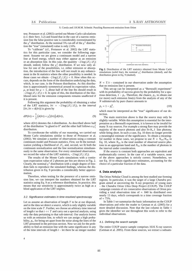
S. Czesla and J.H.M.M. Schmitt: Puzzling fluorescent emission from Orion
test. Protassov et al. (2002) carried out Monte-Carlo calculations(c.f. their Sect. 3.2) and found that in the case of a narrow emis-sion line the false-positive rate is considerably overestimated bytheχ2 distribution. At the nominal 5% cut-off of theχ2 distribu-tion the “true” (simulated) value is only 2.6%.
To “calibrate” (cf., Protassov et al. 2002) the LRT statis-tics for this particular case, we consider the following argu-ment: Assume we are given a continuum model and a narrowline at fixed energy, which may either appear as an emissionor an absorption line. In this case, the quantity−2 log (L1/L2)should, indeed, follow theχ2
1 distribution. If we now only al-low for one of the possibilities, i.e. either emission or absorp-tion, the introduction of the line will not result in any enhance-ment in the fit statistics where the other possibility is needed. Inthose cases we obtain−2 log (L1/L2) = 0. How often this oc-curs, depends on the form of the distribution underlying thedata,which, in our case, is the Poisson distribution. As this distribu-tion is approximately symmetrical around its expectation value,µ, at least forµ > 1, about half of the line fits should result in−2 log (L1/L2) = 0. In spite of this, the distribution of the like-lihood ratio for the emission components remains unaffected ifit is present.
Following this argument the probability of obtaining a valueof the LRT statistics,lrt = −2 log (L1/L2), in the interval[lrt, lrt + d(lrt)] is given by
dP(lrt) =12
(δ(lrt) + χ2
1(lrt))
d(lrt) , (9)
whereδ(lrt) denotes theδ-distribution. As described above halfof the distribution “is glued to 0” and the other half followsaχ2
1distribution.
To corroborate the validity of our reasoning, we carried outMonte Carlo simulations similar to those of Protassov et al.(2002). We simulate a number of observations using a constantcontinuum model and Poisson statistics. First, we fit the normal-ization yielding a likelihood ofL1, and, second, we fit both thecontinuum normalization and the line normalization simultane-ously to the same observation. For every simulated observation,we record the value of the LRT statistics,−2 log (L1/L2).
The results of the Monte Carlo simulations with a contin-uum expectation value of 2 photons per bin are shown in Fig. 2.Clearly, the nominalχ2 distribution with a single degree of free-dom fails to reproduce the simulated findings, whereas the dis-tribution given in Eq. 9 provides a considerably better approxi-mation.
Therefore, when testing for the presence of a narrow emis-sion line, we can interpret the numbers obtained for the LRTstatistics using Eq. 9 as a reference distribution. In practice, thismeans that our sensitivity is approximately twice as high asablind application of the LRT implies.
3.2. Significance estimates in time-resolved spectroscopy
Let us assume an observation of lengthT to be at our disposal,and in the data we detect a source, which is only slightly variableon the time scaleT . Further, we choose an arbitrary time intervalof lengtht so thatt << T and carry out a spectral analysis, usingonly the data pertaining to that sub-interval. Our analysisleavesus with an emission line, to which we can assign a high proba-bility, pe, for being set apart from the noise along the lines of theLRT presented in the previous section. Now we ask for the prob-ability to find an emission line with the same significance in anyof the time intervals of lengtht – let there be an integer number
0 1 2 3 4 5
Likelihood ratio test statistics
0.0
0.2
0.4
0.6
0.8
1.0
CD
F
Simulated distribution21
1
2+
1
2
21
Fig. 2. Distribution of the LRT statistics obtained from Monte Carlosimulations (solid line), the nominalχ2
1 distribution (dotted), and thedistribution given in Eq. 9 (dashed).
N ≈ T/t – contained in our observation under the assumptionthat no emission line is present.
This set-up can be interpreted as a “Bernoulli experiment”with its probability of success given by the probability fora spu-rious detection, 1− pe. Therefore, the chance,ps, to obtain one(or more) such emission line(s) from the analysis of any of theN subintervals by pure chance amounts to
ps = 1− pNe , (10)
which must be interpreted as the “true” significance of our de-tection.
The main restriction above is that the source may only beslightly variable. While this assumption is essential for the inter-pretation as a Bernoulli experiment, it is known to be invalid formany X-ray sources. For example a strong flare may provide themajority of the source photons and also Fe Kα I line photons,while being short. In such a case, Eq. 10 does no longer providea meaningful estimate of the significance. To obtain a meaning-ful number in these cases, we propose to useN = Ntot/Nint inEq. 10, whereNtot is the total number of observed source pho-tons in an appropriate band andNint is the number of photons inthe interval under consideration.
If the source is constant both approaches are equivalent andmathematically correct. In the case of a variable source, noneof the above approaches is strictly correct. Nonetheless, weuse Eq. 10 to obtain significance estimators, accounting forthechoice of a particular fraction of the data.
4. Data analysis
The Orion Nebular Cloud is among the best studied star formingregions. In particular, it was the target of a largeChandra pro-gram aimed at uncovering the X-ray properties of young stars– theChandra Orion Ultra Deep Project (COUP). The COUPcampaign consists of six consecutive observations of Orionpro-viding a total observation time of≈ 840 ks distributed overnearly 13 days, which corresponds to a time coverage fractionof ≈ 75%.
In Table 1 we summarize the basic information on the COUPobservations and refer the reader to Getman et al. (2005) foramore detailed discussion. Note that the last column in Table1gives the identifier we use throughout this work to refer to theindividual observations.
4.1. Defining the search sample
The entire COUP source sample comprises 1616 X-ray sources(Getman et al. 2005). From these sources, we extract a subsam-
4
3.6 Publications 3 X-RAY ASTRONOMY
46

S. Czesla and J.H.M.M. Schmitt: Puzzling fluorescent emission from Orion
Table 1. The COUP observations.
Obs. ID Start [ks]a Length [ks] Identifier4395 0 100 O13744 156 164 O24373 384 172 O34374 616 169 O44396 841 165 O53498 1070 69 O6
a Counted from MJD 52647.9.
ple used in our search for the fluorescent Fe Kα I line. Since theline has a fixed energy of 6.4 keV, it is advisable to include onlythose sources, which show a sufficient number of counts in anappropriate energy interval around 6.4 keV.
In our analysis we use only sources with more than 30 countsin the “emission-band” (6.2−6.5 keV). In particular, we iteratedthrough the sources presented by Getman et al. (2005), extractedthe source counts in the emission band, corrected them for thePSF coverage of our extraction region, and included the sourcewhen our search criterion was matched.
For the weakest source included in the sample of Tsujimotoet al. (2005) (COUP 649), we find 31 emission band photons,making our sample include the Tsujimoto et al. sources as a sub-sample.
Our final sample comprises a total of 108 COUP sources,which provide the the most promising candidates for our searchfor fluorescent emission. For our purpose, COUP 123 andCOUP 124 collapse into a single source, because they are ei-ther too close to be resolved (1.4 arcsec,≈ 5 arcmin off-axis), ora single source. Their spectrum is appropriately describedby asingle temperature thermal model.
Additionally, we had to exclude COUP 90 and COUP 828from our sample, because they are located on chip edges, whichprevented us from obtaining appropriate spectra (CIAO 4.1), sothat the sample size reduces to 106 COUP sources.
4.2. Extraction regions and pile-up
For most of our sources we use circular extraction regions cover-ing the entire source. Our search sample necessarily contains themost X-ray luminous sources in the COUP field, which may suf-fer from severe pile-up. To avoid a strong pile-up effect, we useannulus shaped extraction regions in 29 cases. Whether pile-upbecomes severe depends not only on the source count rate, butalso on its temporal behavior and positioning on the detector. Wechose the annulus parameters in accordance with these consid-erations, and note whenever an annulus shaped region was usedfor extraction.
4.3. A standard analysis
Our search sample consists of 106 sources. To achieve a homo-geneous scan for the fluorescent Fe Kα I line, they should betreated using standard criteria, eliminating biases arising fromindividual, subjective choices during the analysis.
4.3.1. Bayesian block analysis of the broad-band light curves
A key ingredient in the LLC method is the determination of thecorrect continuum ratio. The observed count rate for individ-ual X-ray sources can vary by orders of magnitude during the
COUP campaign. Although the continuum ratio is relatively ro-bust against temperature variations (see Sec. 2.3), it is advisableto distinguish between periods of different count rate regimes,possibly indicating different source spectra and continuum ra-tios. Of course a transition between different spectra may notalways be accompanied by a count rate change, but we neglectthis possibility here.
Our count rate analysis is based on the broad-band (2−9 keV)light curve. To separate the entire campaign data of individualsources into intervals with comparable count rate, we applytheconcept of “Bayesian blocks” elaborated by Scargle (1998).Themethod of Bayesian blocks ‘converts raw photon counts into themost probable piecewise constant representation of brightness asa function of time’ (Scargle 1998).
We apply an iterative algorithm to find individual changepoints in the light curves. This, according to Scargle (1998), doesnot represent the exact mathematical treatment of the problem,but, nonetheless, yields comparable results. As was pointed outby Scargle, an appropriate condition must be found to stop theiteration before segmenting the data set excessively. Instead ofapplying the Bayes factor (Eq. 48 in Scargle 1998) and a prior,we use the likelihood ratio, which can be easily calculated,todecide whether to introduce a change point or not.
As the continuum ratio depends only weakly on the spectraltemperature, we aim at a coarse segmentation of the light curvesin order to separate periods between which the spectrum of theassociated source may significantly differ and with it the contin-uum ratio. To introduce a change point, we demand no less than100 counts per block, a minimum block length of 20 ks, and avalue of the LRT statistics larger than 100.
With this method we separate the 106 source light curvesinto 419 intervals of comparable count rate, and proceed by gen-erating spectra for every individual source and block, which canbe used to determine the corresponding continuum ratio.
4.3.2. Automated model fits
For our analysis we use both thermal as well as power law mod-els, for which we set up automated fit procedures using XSPEC.
The fits of the thermal model are based on the 0.3 − 9 keVenergy band. As a basis for our fits, we use an absorbed two-temperature APEC (e.g. Smith et al. 2001) model extended byan emission line representing the fluorescent Fe Kα I line at6.4 keV. Additionally, we allow for emission lines at variousother energies, which are later used to substantiate our results.The nominal intrinsic width of all lines is 0 eV. All element abun-dances but that of iron are treated as a single fit parameter, whichis also shared among the two thermal components. In contrast,the iron abundance represents an independent fit parameter inboth thermal components.
Starting a fit process with unfavorable initial conditions caneasily lead to unphysical results, even if the fit converges appro-priately. Therefore, the process must be set up carefully toavoidconverging to unrealistic solutions.
Our approach is the following: We start using only one ofthe two available thermal components and than add in the sec-ond. If the enhancement in C-statistics exceeds 6.4 by introduc-ing the the later component, this solution is kept, otherwise theone temperature solution is used. The value of 6.4 correspondsto the 90% cut-off in a likelihood ratio test comparing modelswhich differ by 3 degrees of freedom, which are temperature,iron abundance, and normalization here. We note that the numer-ical equality with the fluorescent line energy is purely accidental.
5
3 X-RAY ASTRONOMY 3.6 Publications
47

S. Czesla and J.H.M.M. Schmitt: Puzzling fluorescent emission from Orion
Furthermore, we apply a number of restrictions to the tem-peratures and abundances to avoid unphysical solutions. Ifthetemperature of any thermal component exceeds 8 keV, we fix itat 8 keV and reiterate the fit, because temperatures beyond thislimit can hardly be resolved inChandra ACIS I spectra. If oneof the iron abundances exceeds 10 times the solar value, it isfixed to the value of the global abundance pattern, because itisusually not well constrained in this case. Similarly, the globalabundances are fixed at solar values, if the fit result is foundtoexceed 10 times the solar value.
After an acceptable solution is found, we obtain fluxes andequivalent widths for the fluorescent line and the comparisonline on the basis of these fits. Finally, the fits are used to derivethe continuum ratio for the Bayesian block under consideration.In this vein, effective area and absorption are automatically ac-counted for in its derivation.
To complement the results of the thermal model, we alsoadapt an absorbed power law model using only the high energytail (3 − 9 keV band) of the spectra. This model is extended bynarrow emission lines accounting for the Fe Kα I line at 6.4 keVand the hot iron line complex at 6.7 keV.
The results of these fits are particularly interesting as theyyield the EW of the hot iron line complex, and they providemeans to check whether the adaption of the thermal modelfailed.
4.3.3. Line light curve analysis
As soon as the continuum ratios are determined, the LLC and theCLLC can be calculated. According to our reasoning, periodsofbona fide fluorescent emission are characterized by an increasein the CLLC. Taking an impartial position, the morphology ofthe increase is unknown. Neither can we say on what time scalesthe CLLC typically evolves, nor can we say whether the rise iscontinuous or not, or whether it is correlated with the soft X-raycontinuum.
In our search for candidate intervals, we first exclude thosesources, which do not show a CLLC excess larger than the ex-pected one (cf. Eq. 7). For each remaining source, we search allconceivable connected intervals longer than 20 ks for the largestrelative excess in fluorescent photons. About 4 000 of such in-tervals can be constructed considering that we have 89 bins of≈ 10 ks length each. For each of these conceivable intervals, wecalculate the quantityNσ defined by
Nσ =∑
i LLCi√∑i
Nc,i(∆t)i
rc,i
. (11)
wherei is an index running over all light curve bins in the inter-val, Nc is the observed rate of comparison band photons,rc thecontinuum ratio, and∆t is the duration of the individual bins.As an additional constraint, we demand that each interval tobeconsidered must at least comprise 5 CLLC excess photons and≥ 50 comparison band photons to be relevant.
The most promising candidate interval is that with the high-est Nσ value. Yet, as every source will contain one such inter-val, we have to choose a reasonable limit forNσ; only beyondthis limit intervals shall be considered valid candidate intervals.Replacing the Poisson distributions by normal distributions, itmay be shown thatNσ approximately follows a standard normaldistribution. Therefore, the probability thatmax(Nσ) exceeds alimit, L, becomes
p(max(Nσ) > L) = 1− Normal0,1(Nσ < L)n , (12)
wheren is the number of intervals for whichNσ is determinedandNormal0,1 denotes the standard normal distribution. If, as inour case,n is≈ 4000 and we demandp(max(Nσ) > L) = 0.2, weobtainL ≈ 3.9, which is considered a reasonable limit forNσ.The preceding approximation does not take into account, thatmost intervals overlap and are, therefore, not independent, andit also neglects, that some may not contain enough photons tobe relevant. To overcome these shortcoming, we obtain a moreappropriate limit by a Monte Carlo simulation. For each source,we simulate a number of light curves based on Poisson statisticwith the observation as our expectation value. From these artifi-cial light curves a distribution ofmax(Nσ) can be derived, whichtakes into account all constraints. We note, however, that the thusobtained results are in good agreement with the approximation.
Following the above stated approach, we find candidate in-tervals in 25 of our sample sources, and we proceed by ex-tracting the associated spectra. We then apply the same auto-mated thermal fits as above to find a spectral model. On the ba-sis of this model, we calculate the significance of the fluores-cent Fe Kα I line in the interval using Eq. 9 and apply Eq. 10 toaccount for our interval choice. We evaluate Eq. 10 using bothdefinitions of the number of repetitions in the Bernoulli experi-ment, i.e., interval length and the number of enclosed photons.The maximum of both results is used as a significance estima-tor. We prefer the maximum to the more conservative minimumhere, because latter would necessarily underestimate the signif-icance during a flare, which is typically short but intense. Wealso note that the application of Eq. 10 is no longer fully jus-tified here, because the “experiments” are not fully independentwhen a distinguished interval is chosen in advance. Nonetheless,the number is used as an estimate.
In Table 2 we list those sources with a line detection at a sig-nificance level of≥ 95%. Our sample comprises 23 sources in-cluding 6 sources already reported on by Tsujimoto et al. (2005).Note that we excluded COUP 554 from the list, because a cor-rect analysis of this source was impeded by pile-up. Consultingthe 95% limit, we estimate that 1− 2 detection given in Table 2must be attributed to noise. Taking into account the difficulties indefining the true significance of the Fe Kα I line in this tempo-rally resolved analysis, we note that also accepting 3−4 spuriousdetections, does not seriously alter the outcome of the analysis.
5. Discussion
This section starts with a presentation of individual sources, pro-ceeds with an analysis of several sample properties, and, finally,closes with a discussion dedicated to the physical scenarioofFe Kα I line creation in the light of our results.
5.1. Previously known COUP sources with fluorescentemission
Tsujimoto et al. (2005) present a sample of 7 COUP sources(COUP sequence nos. 331, 561, 621, 647, 649, 1030, and 1040)with a detection of fluorescent emission. The authors, how-ever, did not carry out time-resolved spectroscopy, but usetime-averaged spectra. Below we present the outcomes obtained forthe Tsujimoto et al. sources to demonstrate the techniques de-veloped so far.
In the following values given in parentheses refer to the 90%confidence range for the given parameter.
6
3.6 Publications 3 X-RAY ASTRONOMY
48

S. Czesla and J.H.M.M. Schmitt: Puzzling fluorescent emission from Orion
Table 2. Most promising intervals for fluorescent emission and basic fit results.
COUPa b Nσ Interval Sign. Fe Kα I EW N6.4keV NH T1 T2
seq. no. [ks] [%] [eV] [10−7 ph/(cm2 s)] [1022 H/cm2] [keV] [keV]7 3.95 60-961 99.99 446(216-667) 2.48(1.20-3.71) 0.02(0.01-0.03) 2.08(1.97-2.34) 0.83(0.81-0.85)9 3.86 514-851 99.35 366(123-628) 7.95(2.67-13.63) 0.19(0.15-0.22) 3.72(3.12-5.14) 1.00(0.89-1.07)245a 5.32 80-891 99.98 482(261-906) 1.90(1.03-3.57) 0.16(0.10-0.20) 4.51(3.60-8.23) 0.84(0.77-1.00)267 4.81 30-196 99.88 400(176-672) 13.02(5.73-21.88) 2.42(2.15-2.61) 8.00 -331b 6.92 1080-1110 100 1437(959-1927) 78.9(52.7-105.8) 1.79(1.60-2.00) 8.00 -449 3.67 296-961 98.69 212(60-391) 1.62(0.46-2.98) 1.53(1.29-1.76) 2.87(2.41-3.47) 0.98(0.76-1.13)561b 4.64 100-414 99.98 569(279-914) 4.60(2.25-7.38) 0.98(0.90-1.07) 2.40(2.20-2.64) -599 4.65 10-1080 99.99 448(216-663) 2.07(1.00-3.06) 7.64(6.65-8.75) 3.67(2.86-4.89) -621b 6.21 10-296 99.97 602(307-973) 4.84(2.47-7.83) 4.54(4.29-5.24) 3.25(2.64-4.98) 0.08(0.00-0.09)647b 4.22 50-626 99.85 440(194-767) 3.42(1.51-5.96) 25.23(20.33-31.63) 5.87(3.69-9.32) -662 4.09 246-394 98.35 206(93-434) 12.61(5.70-26.57) 16.06(14.40-17.88) 8.00 0.08(0.00-0.11)669 4.39 384-776 99.88 384(160-616) 2.73(1.14-4.38) 0.33(0.29-0.36) 8.00 1.02(0.95-1.06)680 4.21 80-716 99.94 410(190-689) 2.25(1.04-3.77) 11.63(9.68-13.41) 8.00 0.08(0.00-0.09)682 3.53 851-1130 98.62 312(108-591) 3.01(1.04-5.71) 1.52(1.22-1.76) 3.05(2.71-3.71) 0.09(0.00-0.11)797a 3.26 20-951 96.85 82(11-151) 3.28(0.45-6.08) 29.04(27.23-30.92) 8.00 -801 4.79 166-636 99.54 456(163-785) 5.91(2.11-10.20) 0.41(0.36-0.48) 3.08(2.40-4.25) 1.04(0.89-1.23)942 3.90 286-716 99.99 308(173-506) 4.68(2.62-7.69) 1.08(0.99-1.15) 3.44(3.16-3.87) -1030a,b 3.17 206-716 99.68 143(56-231) 6.35(2.50-10.25) 16.14(13.85-18.68) 8.00 0.28(0.22-0.33)1035 4.09 394-686 98.26 410(153-851) 2.78(1.04-5.77) 1.76(1.59-2.02) 2.24(1.92-2.53) -1040b 3.80 266-544 98.62 307(110-664) 3.14(1.12-6.78) 1.44(1.29-1.60) 2.95(2.58-3.46) -1080 4.35 766-961 98.58 332(107-578) 6.99(2.26-12.19) 2.35(1.95-2.86) 3.28(2.68-3.86) 0.63(0.00-0.88)1380 3.95 554-786 96.37 187(49-336) 5.68(1.49-10.21) 0.51(0.45-0.59) 8.00 1.15(0.93-1.47)1499 4.50 384-524 99.69 372(145-631) 7.25(2.83-12.30) 0.43(0.37-0.49) 4.56(3.88-5.40) -
a Annulus shaped source region.b Sources present in the sample of Tsujimoto et al. (2005).
5.1.1. COUP 331 - V 1486 Ori
This source was already discussed in detail in a previous publica-tion by Czesla & Schmitt (2007). V 1486 Ori shows two majorflare events during the COUP campaign. The first, rather shortone, takes place towards the end of O1 (“Flare I” in Czesla &Schmitt 2007); no significant fluorescent Fe Kα I line emissionwas detected here.
In Fig. 3 (panel A) we show the broad-band light curve, thechange points returned by the Bayesian analysis, and the result-ing CLLC. The first flare is not accompanied by a considerableexcess in the CLLC. The spectrum is well fitted by an absorbedthermal model with a strong (hot) iron line complex at≈ 6.7 keV.
The CLLC clearly indicates that the fluorescent Fe Kα I lineemission is present during the rise-phase of a second, moreviolent flare ignited during O6, which is in line with previ-ous findings (Czesla & Schmitt 2007). The automated searchfor intervals with fluorescent Fe Kα I emission returned the1080− 1110 ks period (cf. Table 2) as the most promising can-didate interval. In Fig. 4 we present the LLC and the spectrumfor the corresponding part of the observation. The LLC clearlyshows the concentration of Fe Kα I line emission in the risephase of the flare, and the spectral analysis yields an EW of1440(960− 1930) eV for the line.
The measured EW of this Fe Kα I line exceeds typical modelpredictions (see Sect. 6) by an order of magnitude, and it is,thus, particularly interesting. A more detailed discussion aboutthe origin of this Fe Kα I line is given later in Sect. 6.3.
5.1.2. COUP 561
Figure 3 (B) shows the results of our light curve analysis forCOUP 561. The CLLC shows two phases of increase. During thesecond COUP observation, as in the longest part of the COUP
-1 0 1 2 3 4 5 6 7
1060 1070 1080 1090 1100 1110 1120 1130
(Sca
led)
cou
nts
Time [ks]
LLC2-9 keV LC
6 6.4 6.8020406080100120140160180
Cou
nts/
keV
Energy [keV]
Fig. 4. Left: LLC and (scaled) broad-band light curve (2.5 ks binning)for COUP 331 (O6). Right: Excerpt of the spectrum (corresponding tothe gray shaded time span in the left panel). Both a model with andwithout extra line emission are indicated.
campaign, COUP 561 is encountered in a quiescent state tojudge from the BBLC. Nonetheless, the CLLC indicates about10 excess photons in the emission band.
-2
-1
0
1
2
3
4
5
-100 0 100 200 300 400 500 600
(Sca
led)
cou
nts
Time [ks]
LLC2-9 keV LC
6 6.4 6.80
20
40
60
80
100
120
140
Cou
nts/
keV
Energy [keV]
Fig. 5. Left panel: The LLC and the broad-band light curve (both 10 ksbinning) of COUP 561. Latter scaled to show the same maximal countrate as the LLC. The gray shaded area denotes the time span for whichan excerpt of the spectrum is shown in the right panel. There weshow the X-ray spectrum around 6.4 keV and indicate both a thermalmodel with and without excess emission at the energy of the fluorescentFe Kα I line.
7
3 X-RAY ASTRONOMY 3.6 Publications
49

S. Czesla and J.H.M.M. Schmitt: Puzzling fluorescent emission from Orion
0
40
80
120
160
|-----O1-----| |---------O2---------| |----------O3----------| |----------O4----------| |----------O5----------| |----O6----|
Cou
nt r
ate
[/ks]
COUP 331 - V 1486 Ori
I1 I2 I3 I4
(A)|-----O1-----| |---------O2---------| |----------O3----------| |----------O4----------| |----------O5----------| |----O6----|
COUP 331 - V 1486 Ori
-5
0
5
10
15
20
0 200 400 600 800 1000
Time [ks] (from MJD 52647.9)
Cum
ulat
ed L
LC[c
ount
s]
-5
0
5
10
15
20
0 200 400 600 800 1000
Time [ks] (from MJD 52647.9)
Cum
ulat
ed L
LC[c
ount
s]
-5
0
5
10
15
20
0 200 400 600 800 1000
Time [ks] (from MJD 52647.9)
Cum
ulat
ed L
LC[c
ount
s]
-5
0
5
10
15
20
0 200 400 600 800 1000
Time [ks] (from MJD 52647.9)
Cum
ulat
ed L
LC[c
ount
s]
-5
0
5
10
15
20
0 200 400 600 800 1000
Time [ks] (from MJD 52647.9)
Cum
ulat
ed L
LC[c
ount
s]C
umul
ated
LLC
[cou
nts]
0
20
40
60
80
|-----O1-----| |---------O2---------| |----------O3----------| |----------O4----------| |----------O5----------| |----O6----|
Cou
nt r
ate
[/ks]
COUP 561
I1 I2 I3 I4
(B)|-----O1-----| |---------O2---------| |----------O3----------| |----------O4----------| |----------O5----------| |----O6----|
COUP 561
-5
0
5
10
15
20
25
0 200 400 600 800 1000
Time [ks] (from MJD 52647.9)
Cum
ulat
ed L
LC[c
ount
s]
-5
0
5
10
15
20
25
0 200 400 600 800 1000
Time [ks] (from MJD 52647.9)
Cum
ulat
ed L
LC[c
ount
s]
-5
0
5
10
15
20
25
0 200 400 600 800 1000
Time [ks] (from MJD 52647.9)
Cum
ulat
ed L
LC[c
ount
s]
-5
0
5
10
15
20
25
0 200 400 600 800 1000
Time [ks] (from MJD 52647.9)
Cum
ulat
ed L
LC[c
ount
s]
-5
0
5
10
15
20
25
0 200 400 600 800 1000
Time [ks] (from MJD 52647.9)
Cum
ulat
ed L
LC[c
ount
s]C
umul
ated
LLC
[cou
nts]
0
5
10
15
20
25|-----O1-----| |---------O2---------| |----------O3----------| |----------O4----------| |----------O5----------| |----O6----|
Cou
nt r
ate
[/ks]
COUP 621
I1 I2 I3 I4 I5
(C)|-----O1-----| |---------O2---------| |----------O3----------| |----------O4----------| |----------O5----------| |----O6----|
COUP 621
-5
0
5
10
15
20
25
0 200 400 600 800 1000
Time [ks] (from MJD 52647.9)
Cum
ulat
ed L
LC[c
ount
s]
-5
0
5
10
15
20
25
0 200 400 600 800 1000
Time [ks] (from MJD 52647.9)
Cum
ulat
ed L
LC[c
ount
s]
-5
0
5
10
15
20
25
0 200 400 600 800 1000
Time [ks] (from MJD 52647.9)
Cum
ulat
ed L
LC[c
ount
s]
-5
0
5
10
15
20
25
0 200 400 600 800 1000
Time [ks] (from MJD 52647.9)
Cum
ulat
ed L
LC[c
ount
s]
-5
0
5
10
15
20
25
0 200 400 600 800 1000
Time [ks] (from MJD 52647.9)
Cum
ulat
ed L
LC[c
ount
s]C
umul
ated
LLC
[cou
nts]
0
5
10
15
20
25|-----O1-----| |---------O2---------| |----------O3----------| |----------O4----------| |----------O5----------| |----O6----|
Cou
nt r
ate
[/ks]
COUP 647
I1 I2
(D)|-----O1-----| |---------O2---------| |----------O3----------| |----------O4----------| |----------O5----------| |----O6----|
COUP 647
-5
0
5
10
15
20
0 200 400 600 800 1000
Time [ks] (from MJD 52647.9)
Cum
ulat
ed L
LC[c
ount
s]-5
0
5
10
15
20
0 200 400 600 800 1000
Time [ks] (from MJD 52647.9)
Cum
ulat
ed L
LC[c
ount
s]-5
0
5
10
15
20
0 200 400 600 800 1000
Time [ks] (from MJD 52647.9)
Cum
ulat
ed L
LC[c
ount
s]-5
0
5
10
15
20
0 200 400 600 800 1000
Time [ks] (from MJD 52647.9)
Cum
ulat
ed L
LC[c
ount
s]-5
0
5
10
15
20
0 200 400 600 800 1000
Time [ks] (from MJD 52647.9)
Cum
ulat
ed L
LC[c
ount
s]C
umul
ated
LLC
[cou
nts]
0
10
20
30
40
|-----O1-----| |---------O2---------| |----------O3----------| |----------O4----------| |----------O5----------| |----O6----|
Cou
nt r
ate
[/ks]
COUP 649
I1 I2 I3 I4 I5
(E)|-----O1-----| |---------O2---------| |----------O3----------| |----------O4----------| |----------O5----------| |----O6----|
COUP 649
-5
0
5
0 200 400 600 800 1000
Time [ks] (from MJD 52647.9)
Cum
ulat
ed L
LC[c
ount
s]
-5
0
5
0 200 400 600 800 1000
Time [ks] (from MJD 52647.9)
Cum
ulat
ed L
LC[c
ount
s]
-5
0
5
0 200 400 600 800 1000
Time [ks] (from MJD 52647.9)
Cum
ulat
ed L
LC[c
ount
s]
-5
0
5
0 200 400 600 800 1000
Time [ks] (from MJD 52647.9)
Cum
ulat
ed L
LC[c
ount
s]
-5
0
5
0 200 400 600 800 1000
Time [ks] (from MJD 52647.9)
Cum
ulat
ed L
LC[c
ount
s]C
umul
ated
LLC
[cou
nts]
0
20
40
60
80
|-----O1-----| |---------O2---------| |----------O3----------| |----------O4----------| |----------O5----------| |----O6----|
Cou
nt r
ate
[/ks]
COUP 1030
I1 I2 I3 I4 I5
(F)|-----O1-----| |---------O2---------| |----------O3----------| |----------O4----------| |----------O5----------| |----O6----|
COUP 1030
-5
0
5
10
15
20
25
0 200 400 600 800 1000
Time [ks] (from MJD 52647.9)
Cum
ulat
ed L
LC[c
ount
s]
-5
0
5
10
15
20
25
0 200 400 600 800 1000
Time [ks] (from MJD 52647.9)
Cum
ulat
ed L
LC[c
ount
s]
-5
0
5
10
15
20
25
0 200 400 600 800 1000
Time [ks] (from MJD 52647.9)
Cum
ulat
ed L
LC[c
ount
s]
-5
0
5
10
15
20
25
0 200 400 600 800 1000
Time [ks] (from MJD 52647.9)
Cum
ulat
ed L
LC[c
ount
s]
-5
0
5
10
15
20
25
0 200 400 600 800 1000
Time [ks] (from MJD 52647.9)
Cum
ulat
ed L
LC[c
ount
s]C
umul
ated
LLC
[cou
nts]
0
55
110
165
220
|-----O1-----| |---------O2---------| |----------O3----------| |----------O4----------| |----------O5----------| |----O6----|
Cou
nt r
ate
[/ks]
COUP 1040
I1 I2 I3 I4
(G)|-----O1-----| |---------O2---------| |----------O3----------| |----------O4----------| |----------O5----------| |----O6----|
COUP 1040
-5
0
5
10
15
20
0 200 400 600 800 1000
Time [ks] (from MJD 52647.9)
Cum
ulat
ed L
LC[c
ount
s]
-5
0
5
10
15
20
0 200 400 600 800 1000
Time [ks] (from MJD 52647.9)
Cum
ulat
ed L
LC[c
ount
s]
-5
0
5
10
15
20
0 200 400 600 800 1000
Time [ks] (from MJD 52647.9)
Cum
ulat
ed L
LC[c
ount
s]
-5
0
5
10
15
20
0 200 400 600 800 1000
Time [ks] (from MJD 52647.9)
Cum
ulat
ed L
LC[c
ount
s]
-5
0
5
10
15
20
0 200 400 600 800 1000
Time [ks] (from MJD 52647.9)
Cum
ulat
ed L
LC[c
ount
s]C
umul
ated
LLC
[cou
nts]
Fig. 3. Panel A to G: Light curves for the objects reported on by Tsujimoto et al. (2005). The time axis refers to the begin of the COUP campaign(MJD 52647.87). Upper panel: Broad-band (2− 9 keV) light curve (BBLC). Lower panel: The cumulated LLC (CLLC) and an estimate of itswidth (gray shaded, see Eq. 7). Vertical separators mark change points associated with a shift of the activity level (determined by the Bayesianblock analysis of the BBLC).
In Fig. 5 (left panel) we show the LLC pertaining the firsthalf of the COUP campaign, and the most promising candidateinterval (100− 414 ks) for fluorescent emission is gray shaded.In the right panel we plot the spectrum obtained for this interval,which shows a fluorescent line with an EW of 570(280−910) eV.The hot iron-line complex is virtually absent.
During the flare in the following observation, the CLLCindicates another increase by about 10 photons. This num-
ber is confirmed by a spectral analysis of the associated span(504− 544 ks), where we find a Fe Kα I line with an EW of132(12− 270) eV. Because of the larger flare continuum the lineis much less prominent here, and with 96% it is also much lesssignificant.
8
3.6 Publications 3 X-RAY ASTRONOMY
50

S. Czesla and J.H.M.M. Schmitt: Puzzling fluorescent emission from Orion
5.1.3. COUP 621
The outcome of the light curve analysis for COUP 621 is shownin Fig. 3 (C). COUP 621 shows two flares with the first one fullycovered by the observation (except for a probably small fractionof the rise-phase) and the second one remaining unobserved for≈ 60 ks of its central phase. None of these flares is accompaniedby a CLLC excess. The CLLC shows an increase, which is notassociated with one of the flares, but rather emerges during aperiod of quiescence to judge from the BBLC.
-2
0
2
4
6
8
0 100 200 300 400 500
(Sca
led)
cou
nts
Time [ks]
LLC2-9 keV LC
6 6.4 6.80
20
40
60
80
100
120
Cou
nts/
keV
Energy [keV]
Fig. 6. COUP 621; as in Fig. 5
In Fig. 6 we show the LLC corresponding to O2 and O3 inthe left panel where we also indicate the most promising interval(cf. Table 2). In the right panel we show the associated spectrum.Excess emission at the location of the fluorescent line is promi-nent with a line EW of 600(310− 970) eV, and the hot iron linecomplex is weak compared to it.
This case is special because two flares detected in soft X-raysare not accompanied by fluorescent Fe Kα I line emission, whilethere is a line detection during a period preceding the first flare.The line emission may be attributed to a hidden flare locatedat a geometrically quite favorable position. At least it must beattributed to an event, which does not show up in soft X-rays.
5.1.4. COUP 647
Among the sources analyzed by Tsujimoto et al. COUP 647 isby far the most deeply embedded one with a hydrogen columndensity of≈ 31 × 1022 cm−2.
The CLLC shows two phases of increase. One associatedwith a flare towards the end of the COUP campaign, and anotherone earlier in a presumably quiescent phase of the source (seeFig. 3 D). Our automated CLLC analysis returns the first phase,in particular the 50−626 ks interval, as the most promising can-didate interval, for which we show the spectrum in the left panelof Fig. 7. The EW of the line in this phase is 440(194− 767) eV.
Additionally, we show the spectrum of the flare during whichthe line shows up with an EW of 150(10− 300) eV.
6 6.4 6.80
40
80
120
160
200
Cou
nts/
keV
Energy [keV]
6 6.4 6.80
40
80
120
160
200
Cou
nts/
keV
Energy [keV]
Fig. 7. Left panel: excerpt of the spectrum during the bona fide quies-cent phase of COUP 647. Right panel: The same part of the spectrumduring the flare.
5.1.5. COUP 649
Among the sources of fluorescent emission reported on byTsujimoto et al. (2005), COUP 649 is the one with the weak-est Fe Kα I line.
Figure 3 (E) shows the BBLC and the associated CLLC. Thesource signal is dominated by a single flare, beyond which thesource is virtually invisible. This source was rejected by our au-tomated analysis, because the determined excess is not sufficientto fulfill our criteria. The light curve of COUP 649 shows rapidvariability where the source is visible, and we speculate that thisimpedes an appropriate light curve analysis.
In a spectral analysis of the flare, however, we find a fluores-cent emission with an EW of≈ 260(80− 450) eV, compatiblewith the results given by Tsujimoto et al. (2005). We note that,in this case, the EW is not affected by time averaging, becauseonly the flare contributes signal.
5.1.6. COUP 1030
Figure 3 (F) shows the light curves pertaining to COUP 1030.A flare occurs in O4, and we find that the source is piled-up inthis state. In the following analysis we, therefore, revertto anannulus-shaped source region neglecting the innermost 0.6 arc-sec.
-4
-2
0
2
4
6
640 660 680 700 720 740 760 780 800
(Sca
led)
cou
nts
Time [ks]
LLC2-9 keV LC
6 6.4 6.80
100
200
300
400
500
Cou
nts/
keV
Energy [keV]
Fig. 8. COUP 1030; as in Fig. 5
The automated CLLC analysis yields the 206− 716 ks inter-val to be the most promising to detect fluorescent Fe Kα I emis-sion. This interval covers the flare, which, according to theCLLC, provides the largest contribution of fluorescent photons.In the right panel of Fig. 8 we show the spectrum of COUP 1030during the most promising interval, and our spectral analysisshows a fluorescent line with an EW of 143(56− 231) eV. Theresult is compatible with the values given by Tsujimoto et al.(2005); time averaging has no effect on the EW if the signal isstrongly concentrated in a single flare. This source appearsmuchlike a “text book” example of fluorescent emission originatingfrom photoionization both with respect to temporal behavior andEW.
5.1.7. COUP 1040
COUP 1040 remains virtually invisible in the> 6.2 keV band,except for a flare period during O2.
Figure 3 (G) shows the light curves. The LLC indicates fluo-rescent emission accompanying a flare. There is a steep rise in ashort (≈ 10 ks) interval in the central flare, and the CLLC contin-ues to rise during the decay phase. Our automated analysis de-termines an interval containing the decay phase (266− 544 ks)of the flare to be the most promising candidate interval to besearched for fluorescent Fe Kα I emission. In Fig. 9 (left panel)we show the spectrum pertaining to this interval. Indeed, there
9
3 X-RAY ASTRONOMY 3.6 Publications
51

S. Czesla and J.H.M.M. Schmitt: Puzzling fluorescent emission from Orion
may be excess emission at 6.4 keV, however, the continuum inthe 5.2 − 6.2 keV range is not well fitted by the model, so thatthe CLLC may be misleading in this case.
5.2 5.6 6 6.4 6.80
40
80
120
Cou
nts/
keV
Energy [keV]
6 6.4 6.80
50
100
150
200
250
300
350
Cou
nts/
keV
Energy [keV]
Fig. 9. Left panel: The spectrum during the automatically determined,most promising fluorescent interval of COUP 1040. Right panel: Thespectrum during the second COUP observation (O2).
The right panel of Fig. 9 shows the spectrum during the O2,which covers the flare and its decay phase. The signal is muchstronger here, and the fluorescent line is detectable. While theline flux of 11(6− 20)× 10−7 ph/(cm2 s) is considerably higherthan the value reported by Tsujimoto et al. (2005), our EW of178(90− 310) eV is compatible with their result, as it remainsunchanged by time averaging if no further signal is accumulated.
5.2. Three individual sources with distinct behavior
In the following section we present three additional indi-vidual sources with a detection of fluorescent emission. Thesources show three different types of temporal behavior of theFe Kα I line, and further demonstrate the variety of Fe Kα I lineemitters.
5.2.1. COUP 267
The X-ray spectrum of COUP 267 shows the characteristics ofa “two absorber X-ray source” (TAX source, e.g., Gudel et al.2007), with a mildly absorbed soft component dominating be-low about 1 keV and a hard component hidden behind a signif-icantly higher column of material. During the leading 100 ksofCOUP campaign data, COUP 267 shows a flare (see Fig. 10, up-per panel). A comparison of the soft (0.3− 1.2 keV) light curveand its hard counterpart (1.2 − 9.0 keV) uncovers that the flareexclusively affects the hard band.
In Fig. 10 we show the light curves and the spectrum ofCOUP 267 during the 30−196 ks time span selected by our auto-matic search for fluorescence, which basically covers the decayphase of the flare. The EW of the fluorescent line amounts to400(180− 670) eV here. The two differently absorbed thermalcomponents can clearly be distinguished in the spectral model,and excess emission at the energy of the fluorescent line is vis-ible. The upper right box in Fig. 10 shows a close-up of thisregion, where the best-fit line is also indicated.
The TAX nature of this source implies the presence of con-siderable amounts of circumstellar material surrounding the cen-tral star, where fluorescent emission may well have its origin.Although the measured EW appears high compared to the modelpredictions (see Sect. 6), the fluorescent emission is associatedwith the flare, and we conclude that photoionization provides areasonable explanation for the observation.
0
5
10
15
20
25
30|-----O1-----| |---------O2---------| |----------O3----------| |----------O4----------| |----------O5----------| |----O6----|
Cou
nt r
ate
[/ks]
I1 I2 I3
|-----O1-----| |---------O2---------| |----------O3----------| |----------O4----------| |----------O5----------| |----O6----|
-5
0
5
10
0 200 400 600 800 1000
Time [ks] (from MJD 52647.9)
Cum
ulat
ed L
LC[c
ount
s]
-5
0
5
10
0 200 400 600 800 1000
Time [ks] (from MJD 52647.9)
Cum
ulat
ed L
LC[c
ount
s]
-5
0
5
10
0 200 400 600 800 1000
Time [ks] (from MJD 52647.9)
Cum
ulat
ed L
LC[c
ount
s]
-5
0
5
10
0 200 400 600 800 1000
Time [ks] (from MJD 52647.9)
Cum
ulat
ed L
LC[c
ount
s]
-5
0
5
10
0 200 400 600 800 1000
Time [ks] (from MJD 52647.9)
Cum
ulat
ed L
LC[c
ount
s]C
umul
ated
LLC
[cou
nts]
Fig. 10. Upper panel: The 2− 9 keV band light curve and the CLLC ofCOUP 267. Lower panel: The spectrum during the 30− 196 ks intervalwith a close-up of the Fe Kα I line region.
5.2.2. COUP 599
The strength of the X-ray source COUP 599 remains constantthrough the entire COUP campaign as demonstrated by the lightcurve shown in Fig. 11. The CLLC rises almost without interrup-tion. Accordingly, the most promising fluorescent intervalfoundin our automated search comprises virtually the entire data.
In the lower panel of Fig. 11, we show the spectrum of thesource in the 10− 1080 ks interval. There is excess emissionat 6.4 keV, which we attribute to the fluorescent line, and wedetermine an EW of 450(220− 660) eV for it.
The position of COUP 599 is about 1 arcsec northwest of theBecklin-Neugebauer object (Becklin & Neugebauer 1967), and,as already noted by Garmire et al. (2000) in a pre-COUP study,it may be related to it, although an independent origin cannot beexcluded.
The X-ray luminosity of this source is constant and so is itsFe Kα I line flux. Again, the EW is high compared to valuesrarely exceeding 100 eV as derived by Drake et al. (2008), butthe strong absorption with a column density ofNH = 7.6(6.6 −8.7)× 1022 H/cm2, points towards the presence of circumstellarmaterial, which could yield a quite favorable geometry.
5.2.3. COUP 1499, V NX Ori
While V NX Ori is found in quiescence for the longest part ofthe COUP campaign, it also shows a period of remarkable ac-tivity. This begins with a very short flare taking place towardsthe end of the second observation. Here, the count rate skyrock-ets to about 40 c/ks (2− 9 keV band) within 2 ks and then de-
10
3.6 Publications 3 X-RAY ASTRONOMY
52
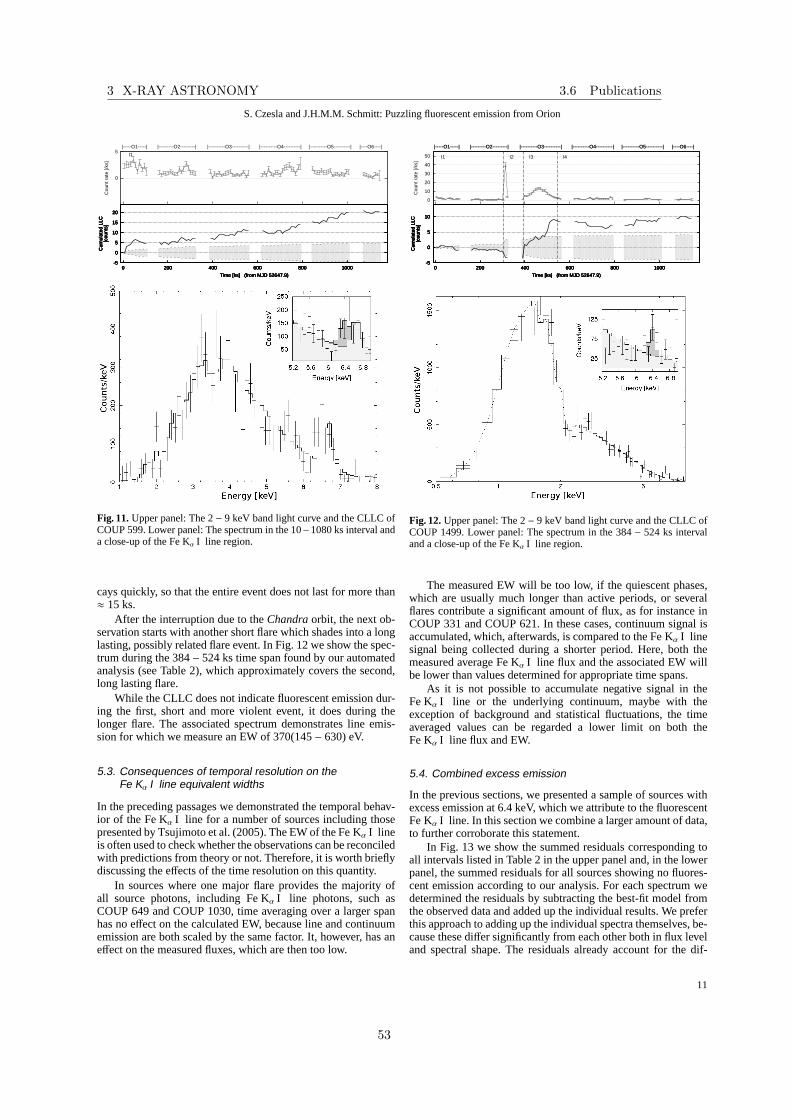
S. Czesla and J.H.M.M. Schmitt: Puzzling fluorescent emission from Orion
0
5|-----O1-----| |---------O2---------| |----------O3----------| |----------O4----------| |----------O5----------| |----O6----|
Cou
nt r
ate
[/ks]
I1
-5
0
5
10
15
20
0 200 400 600 800 1000
Time [ks] (from MJD 52647.9)
Cum
ulat
ed L
LC[c
ount
s]
-5
0
5
10
15
20
0 200 400 600 800 1000
Time [ks] (from MJD 52647.9)
Cum
ulat
ed L
LC[c
ount
s]
-5
0
5
10
15
20
0 200 400 600 800 1000
Time [ks] (from MJD 52647.9)
Cum
ulat
ed L
LC[c
ount
s]
-5
0
5
10
15
20
0 200 400 600 800 1000
Time [ks] (from MJD 52647.9)
Cum
ulat
ed L
LC[c
ount
s]
-5
0
5
10
15
20
0 200 400 600 800 1000
Time [ks] (from MJD 52647.9)
Cum
ulat
ed L
LC[c
ount
s]
Fig. 11. Upper panel: The 2− 9 keV band light curve and the CLLC ofCOUP 599. Lower panel: The spectrum in the 10−1080 ks interval anda close-up of the Fe Kα I line region.
cays quickly, so that the entire event does not last for more than≈ 15 ks.
After the interruption due to theChandra orbit, the next ob-servation starts with another short flare which shades into alonglasting, possibly related flare event. In Fig. 12 we show the spec-trum during the 384− 524 ks time span found by our automatedanalysis (see Table 2), which approximately covers the second,long lasting flare.
While the CLLC does not indicate fluorescent emission dur-ing the first, short and more violent event, it does during thelonger flare. The associated spectrum demonstrates line emis-sion for which we measure an EW of 370(145− 630) eV.
5.3. Consequences of temporal resolution on theFe Kα I line equivalent widths
In the preceding passages we demonstrated the temporal behav-ior of the Fe Kα I line for a number of sources including thosepresented by Tsujimoto et al. (2005). The EW of the Fe Kα I lineis often used to check whether the observations can be reconciledwith predictions from theory or not. Therefore, it is worth brieflydiscussing the effects of the time resolution on this quantity.
In sources where one major flare provides the majority ofall source photons, including Fe Kα I line photons, such asCOUP 649 and COUP 1030, time averaging over a larger spanhas no effect on the calculated EW, because line and continuumemission are both scaled by the same factor. It, however, hasaneffect on the measured fluxes, which are then too low.
0
10
20
30
40
50
|-----O1-----| |---------O2---------| |----------O3----------| |----------O4----------| |----------O5----------| |----O6----|
Cou
nt r
ate
[/ks]
I1 I2 I3 I4
|-----O1-----| |---------O2---------| |----------O3----------| |----------O4----------| |----------O5----------| |----O6----|
-5
0
5
10
0 200 400 600 800 1000
Time [ks] (from MJD 52647.9)
Cum
ulat
ed L
LC[c
ount
s]
-5
0
5
10
0 200 400 600 800 1000
Time [ks] (from MJD 52647.9)
Cum
ulat
ed L
LC[c
ount
s]
-5
0
5
10
0 200 400 600 800 1000
Time [ks] (from MJD 52647.9)
Cum
ulat
ed L
LC[c
ount
s]
-5
0
5
10
0 200 400 600 800 1000
Time [ks] (from MJD 52647.9)
Cum
ulat
ed L
LC[c
ount
s]
-5
0
5
10
0 200 400 600 800 1000
Time [ks] (from MJD 52647.9)
Cum
ulat
ed L
LC[c
ount
s]C
umul
ated
LLC
[cou
nts]
Fig. 12. Upper panel: The 2− 9 keV band light curve and the CLLC ofCOUP 1499. Lower panel: The spectrum in the 384− 524 ks intervaland a close-up of the Fe Kα I line region.
The measured EW will be too low, if the quiescent phases,which are usually much longer than active periods, or severalflares contribute a significant amount of flux, as for instanceinCOUP 331 and COUP 621. In these cases, continuum signal isaccumulated, which, afterwards, is compared to the Fe Kα I linesignal being collected during a shorter period. Here, both themeasured average Fe Kα I line flux and the associated EW willbe lower than values determined for appropriate time spans.
As it is not possible to accumulate negative signal in theFe Kα I line or the underlying continuum, maybe with theexception of background and statistical fluctuations, the timeaveraged values can be regarded a lower limit on both theFe Kα I line flux and EW.
5.4. Combined excess emission
In the previous sections, we presented a sample of sources withexcess emission at 6.4 keV, which we attribute to the fluorescentFe Kα I line. In this section we combine a larger amount of data,to further corroborate this statement.
In Fig. 13 we show the summed residuals corresponding toall intervals listed in Table 2 in the upper panel and, in the lowerpanel, the summed residuals for all sources showing no fluores-cent emission according to our analysis. For each spectrum wedetermined the residuals by subtracting the best-fit model fromthe observed data and added up the individual results. We preferthis approach to adding up the individual spectra themselves, be-cause these differ significantly from each other both in flux leveland spectral shape. The residuals already account for the dif-
11
3 X-RAY ASTRONOMY 3.6 Publications
53

S. Czesla and J.H.M.M. Schmitt: Puzzling fluorescent emission from Orion
ferences in spectral shape, and the contribution of spectrawithmore photons grows with the square root of the photon number,and not linearly as would be the case otherwise.
An emission line feature, which is not accounted for in themodels but present in some or all of the spectra, should lead toan accumulation of residual photons at the respective energy. InFig. 13 we show the result using the residuals with respect tothethermal model (cf. Sec.4.3) and a power law model extended bya Gaussian line of variable width (but< 0.1 keV) and normal-ization at a fixed energy of 6.7 keV to account for the hot ironlines.
In both cases, an excess at 6.4 keV can clearly be identified.We find that this excess is well represented by a Gaussian cen-tered at 6.4 keV. The best-fit width of the Gaussian is 100 eV,which is consistent with an intrinsically narrow, instrumentallybroadened line at the location of the fluorescent Fe Kα I line. Wenote that leaving the central energy as a free fit parameter doesnot alter this result. Depending on the considered energy rangefor the adaption of the Gaussian, and on whether we allow anoffset for the Gaussian line, we find amplitudes of 300−400 pho-tons. Therefore, we argue for the presence of≈ 350 excess pho-tons, which can be attributed to the fluorescent Fe Kα I line inthese spectra. This number can be converted into an average lineEW of roughly 250 eV, which we find in good agreement withprevious results.
-600-400-200
0 200 400 600 800
1000
3.2 3.6 4 4.4 4.8 5.2 5.6 6 6.4 6.8 7.2 7.6 8
Cou
nts
Energy [keV]
(b)
-50
0
50
100
150
Cou
nts
(a)
Fig. 13. The summed residuals from all bona-fide fluorescent intervals(panel a) and the same for all sources not showing intervals with fluores-cent emission (panel b). Solid (black) line: The residuals with respect tothermal models, dashed (red) line: The residuals with respect to a powerlaw model with additional hot iron line at 6.7 keV.
Instead of collecting the residuals only from the periodsof bona-fide fluorescent emission, the collection can also beinverted to comprise only data of those sources in which noFe Kα I line emission was detected. Neither of the resultingcurves, whether calculated with respect to the thermal or thepower law models, shows a distinct feature at 6.4 keV (Fig. 13,lower panel). The residuals collected from the thermal modelsshow a substructure indicating that the average spectral slope istoo steep. Such an effect is not present in the power-law mod-els, which, however, cover a much smaller fraction of the spec-trum. Consulting the power law fit residuals, a small excess of≈ 100 photons at 6.4 keV may still be present, but it is not clearlyset apart from the noise. We note that we also find no surplus of
negative residuals here as would be expected, if we only had re-moved sources showing a positive noise excess from the sample.
5.5. Comparison features at different energies
For the following analysis we revert to the Bayesian block data,i.e., a subdivision made without paying special attention to thepresence or absence of the Fe Kα I line, even though this mightbe the case due to physical reasons. Starting from the best-fitthermal model, we add a narrow emission line at various ener-gies between 5.5 keV and 6.7 keV. For each Bayesian block, werecord the best-fit line fluxes and EWs.
5.4 5.6 5.8 6.0 6.2 6.4 6.6 6.8Emission line energy [keV]
0.0
0.5
1.0
1.5
2.0
2.5
3.0
3.5
Line f
lux [10
7 ph/(cm2 s)]Mean flux
Median flux
Fig. 14. Mean (solid line) and median (dashed line) flux for narrowemission line at various energies.
In Fig. 14 we show the mean and median line flux deter-mined for the emission line, shifting it from 5.5 keV to 6.7 keVin steps of 100 eV. This set-up includes the actual Fe Kα I lineat 6.4 keV as a special case. Both mean and median line flux are> 0 everywhere, since we demand an emission line. We do notexpect any strong features between 5.5 keV and 6.3 keV, so thatthe results can be attributed to the photon noise.
The mean line flux shown in Fig. 14 remains constant untilthe line energy exceeds 6.1 keV, after which the mean flux rises,reaches a maximum at 6.4 keV, and falls again. We note that thedecrease towards 6.7 keV happens because the thermal modelsinclude the hot iron lines. To assure that not a few large valuesdominate the plot, which is conceivable if the mean line flux isconsidered, we also give the median line flux, which is morestable against outliers. At a lower level, the median flux showsthe same basic pattern with a maximum at 6.4 keV. The levelshows that many values are close to zero, reflecting the casesinwhich an absorption line would formally yield a better fit.
At each line energy the statistic for the comparison line isdifferent, because it is affected by the spectral shape and the ef-fective area. Under the hypothesis that there is nothing specialabout the Fe Kα I line energy, so that the majority of our detec-tions should actually be attributed to noise, the derived result isimplausible. If this hypothesis was to be accepted, there shouldbe a gradual evolution of the mean and median line fluxes overthe entire range, which is, indeed, the case until the line energyexceeds 6.1 keV, but not beyond.
The findings summarized in Fig. 14 are compatible with aninstrumentally broadened emission line at 6.4 keV, and we ad-
12
3.6 Publications 3 X-RAY ASTRONOMY
54

S. Czesla and J.H.M.M. Schmitt: Puzzling fluorescent emission from Orion
duce this as a corroboration of our interpretation of the observedexcess emission as fluorescent Fe Kα I line emission, which isdistinct from photon noise.
5.6. Duty cycle of Fe Kα I line emission
In Table 2 we list the sources and time spans, which show sig-nificant Fe Kα I line emission according to our analysis. Thetable comprises 23 sources, with a total observation time of23× 838 ks≈ 19 000 ks. Summing up the interval lengths, wefind that fluorescent emission is detected during≈ 50% of thistime.
Using the entire sample of 106 sources as a reference, fluo-rescent emission is detectable during about 10% of the observa-tion time, and it is distributed among 20% of the sample sources.This consideration does only take into account those sources inwhich fluorescent emission can be claimed with reasonable cer-tainty. Based on the creation scenario of fluorescent emission,it seems likely that the number of fluorescent sources is actu-ally larger, yet a detection cannot be claimed where the signalremains insufficient. The duty cycle derived here should, there-fore, be regarded a minimum, limited by the sensitivity of theinstrument and, of course, our method.
6. On the origin of the Fe K α I line emission
The reality of the fluorescent Fe Kα I line has so far been es-tablished in quite a number of stellar sources. While all authorsagree that neutral or lowly ionized iron gives rise to the photonsmaking up this spectral component, there is still some debatewhether nonthermal electrons contribute to the excitationof theiron ions. In the following, we briefly juxtapose photoionizationand electron collisional excitation regarding the expected EWsand temporal behavior.
6.1. Implications of photoionization
The fluorescent emission caused by photoionized neutral orlowly ionized iron was investigated theoretically by a num-ber of authors. Bai (1979) and Drake et al. (2008) carried outMonte Carlo calculations, simulating solar and stellar flares.George & Fabian (1991) simulated an accretion disk illuminatedwith a power law spectrum, approaching the situation in AGNsources. George & Fabian (1991) obtain typical EWs between100− 200 eV for a centrally illuminated disk using power lawphoton-indices betweenΓ = 1.3−2.3. The EWs obtained by Bai(1979) and Drake et al. (2008) for thermal input spectra tendbesmaller, rarely exceeding 100 eV.
While the above results refer to solar iron abundances of≈ 4 × 10⁻⁵ Fe/H, the Fe Kα I line EW caused by photoionizediron can be increased, when larger iron abundances are assumed(Drake et al. 2008). In an analysis of the correlation betweeniron abundance and Fe Kα I line EW, however, Ballantyne et al.(2002) find that the EW cannot be increased beyond any limit.As already indicated by Bai (1979) (Fig. 4) or Matt et al. (1997),the EW rises linearly for iron abundances of the order of orlower than the solar value beyond which the relation flattens.According to Ballantyne et al. (2002), the maximal obtainableFe Kα I line EW is around 800 eV.
The Fe Kα I line EWs expected from photoionized iron is,thus, of the order of≈ 100 eV and may reach≈ 800 eV undervery favorable conditions. The light curve of the Fe Kα I lineshould be correlated with the light curve of the incident soft
X-ray continuum, but reverberation effects may be present.Assuming a typical scale of 20 AU for the extent of a stellarsource, delays, if present, would be of the order of≈ 10 ks.
High Fe Kα I line EWs and a virtually unpredictable tempo-ral behavior may be obtained, if totally or partially hiddenX-raysources are considered as proposed by Drake et al. (2008). Thecontinuum emission by those sources can contribute to the repro-cessed photon field, but their direct continuum radiation remainsinvisible, so that the measured Fe Kα I line flux may be signif-icant providing a large EW, which appears to be uncorrelatedwith the measured continuum.
6.2. Electron collisional excitation
The subject of electron collisional excitation of the fluores-cent Fe Kα I line was for example investigated by Emslie et al.(1986). These authors calculate the Fe Kα I line photon flux,Φ,due to electron excitation; the result is given in their Eq. 12. Incombination with their Eq. 7, the relation can be recast and writ-ten as
4πR2
AF(> E1)Φ = ωβ(AbFe)
γ − 1γ
Eγ−11
Kν
∫ ∞
χ
E1−γQI(E)dE , (13)
whereAbFe is the iron abundance,γ + 1 is the spectral index ofthe incident electron power law spectrum,E1 is the lower cut-offenergy of the electron spectrum,K = 2.61× 10⁻¹⁸ keV2/cm2,ν = 1.6 × 10⁻⁹ is the conversion factor from keV to erg,χ =7.112 keV is the K-shell ionization energy of neutral iron,ω isthe iron fluorescence yield,β is the branching between Kα andKβ,γ..., QI is the cross section for K-shell ionization by iron (seee.g., Hombourger 1998),R is the distance to the source,F(> E1)is the total injected electron energy flux in ergs/(s cm2), andA isthe area of the flare. We note that in Eq. 13 we already assumedthat there is no hydrogen column between the electron injectionsite and the neutral iron, which corresponds toN∗ = 0 in Emslieet al. (1986).
Assumingγ = 2.1, AbFe = 4 × 10⁻⁵, E1 = 20 keV, and adistance of 450 pc, Eq.13 can be partially evaluated
AF(> E1) ≈ 4.5× 1041 cm2 ergphoton
× Φ , (14)
where AF(> E1) is the incident energy flux in the form ofelectrons in ergs/s. Using Eq.14 we derive that, for the typicalFe Kα I line fluxes of several times 10−7 ph/(cm2 s) measured forthe COUP sources (Tsujimoto et al. 2005), the injected flux ofelectrons in excess of 20 keV should be of the order of 1035 erg/s.
This number is enormous compared to solar values, wherethetotal energy deposited in nonthermal electrons during a flareis of the order of 1032 erg. Even though flares in Orion YSOsmay be ‘several orders of magnitude more powerful than anysolar flare’ (Getman et al. 2008), the energetics remain problem-atic. Using Eq. 17 from Saint-Hilaire & Benz (2005), we esti-mate the amount of thermal energy,Eth, contained in the plasmaof a large flare to be
Eth = 3kbT√
EM2/n2 · f ≈ 1036 erg , (15)
assuming an emission measure of 1055 cm−3, a density ofn =1012 cm−3, a temperature ofkbT = 10 keV, and a filling fac-tor, f , of unity. In their analysis of RHESSI data of mediumsized solar flares, Saint-Hilaire & Benz (2005) concluded thatEth is of the order of the energy contained in nonthermal parti-cles. Extrapolating this result to the Orion flares, we conclude
13
3 X-RAY ASTRONOMY 3.6 Publications
55

S. Czesla and J.H.M.M. Schmitt: Puzzling fluorescent emission from Orion
that currents sufficient to provide significant Fe Kα I line fluxescannot be sustained for longer than a few seconds.
As pointed out by Emslie et al. (1986), a contribution of elec-tron induced fluorescent emission may be observed during theimpulsive phase of a flare. The Fe Kα I line flux due to electroncollisional excitation should be temporally correlated with thehard X-ray flux, which was, indeed observed by Emslie et al.(1986). Such data are, however, not available for Orion, so thatwe cannot revert to this line of argumentation.
Recently, Peterson et al. (2010) presented high resolutionra-dio images of the Algol binary system resolving a large coro-nal loop reaching from one to the other pole of the K giantsecondary, being orientated towards the primary B star. Theauthors modeled the radio emission observed from this loopby assuming synchrotron emission from an electron populationwith a homogeneous density ofne = 10−3 electrons/cm−3 anda power law spectrum so thatn(E) = ne(E/Emin)−3/2 whereEmin = 80 keV. Assuming that the electrons are moving atthe speed of light, we estimate an electron flux of roughly3× 1010 cm · 1000 cm−3 = 3× 10¹³ electrons/cm−2. Further as-suming a loop length of 1012 cm and a radius to loop length ratioof 0.1 (Favata et al. 2005), the electron flux over the entire loopcross section becomes≈ 1035 electrons/cm2. If we attribute anenergy of 100 keV to all of these electrons, the resulting energyflux in form of energetic electrons becomes 1028 erg/s. Althoughthis number is still far below the needed value, we note thatFavata et al. (2005) find evidence for large magnetic loops withhalf lengths of≈ 1012 cm in their analysis of large COUP flares,which may connect the stellar photosphere with a disk. Withoutbeing able to give a detailed physical modeling, we do not ex-clude that under certain conditions sufficient fluxes of energeticelectrons may be sustained in large magnetic structures.
When a population of high energy electrons hits a thick tar-get such as a stellar photosphere, the electrons thermalizein theplasma and heat it. This gives rise to the evaporation of softX-ray emitting loops observed during solar and stellar flares.Inspired by their findings, Giardino et al. (2007) elaborateon amechanism, which can prevent a population of accelerated elec-trons from causing a soft X-ray flare. Basically, the authorssug-gest that, if the plasma density in the flux tube into which theelectrons are injected, is high enough, the electrons do notther-malize in the photosphere, but are decelerated in situ. Duringthis process, energy is deposited in nonthermal hard X-raysandcollisional excitation of heavier ions such as iron, potentially re-sulting in Fe Kα I line photons. Appropriate conditions for thismechanism to work may, indeed, be found in young stars withongoing accretion.
6.3. Putting our analysis into the context
As outlined in Sec. 6, model calculations of the Fe Kα I linestrength based on photoionization rarely predict line EWs>100 eV. Yet, the EWs listed in Table 2 tend to be significantlylarger than 100 eV, even though some may be smaller consider-ing the errors. The values reported in Table 2 are qualitativelycompatible with the numbers published for Elias 29, for whichGiardino et al. (2007) derive EWs of up to≈ 800 eV during theirsecond time segment.
If photoionization is to be held responsible for the line emis-sion, it must explainall of these observations; both the ob-served EW and the temporal behavior. As the observed EWs tendto be higher than typical predictions, this issue should be ad-dressed first. Drake et al. (2008) discuss four ways in which theFe Kα I line EW may be raised. These are supersolar Fe abun-
dances, disk flaring, a contribution of electron collisional excita-tion, and line-of-sight obscuration of the central flaring source.According to Drake et al. disk flaring, which increases the solidangle coverage of the reflector, can increase the expected EWbyfactors< 2, and increasing the iron abundance ensues a roughlylinear response of the line EW. EWs of the order of 400 eV as inthe majority of our detections, are, therefore, within reach with-out reverting to extreme physical conditions. Additionally, wenote that obscuration of the X-ray source does not only increasethe Fe Kα I line EW when the absorber is impenetrable, but alsoif it has only small optical thickness. The reason is that fluores-cent photons at 6.4 keV can be created as the X-rays are passingthe absorber, while continuum photons can only be destroyed.Yaqoob et al. (2010) show, in a different context, that the op-tically thin approximation for the fluorescence problem breaksdown for column densities as low as≈ 2 × 10²² H/cm2, whichshould also be the scale on which this effect may become notice-able. The effect may well be responsible for a fraction of the ob-served EW in sources with sufficiently large absorbing columns,i.e., in about half of our sources (see Table 2).
The most extreme Fe Kα I line is observed during the risephase of a flare in V 1486 Ori, where we determine a line EWof ≈ 1400 eV (see Sect. 5.1.1) exceeding typical model predic-tions by an order of magnitude. To explain this measurement inthe frame of photoionization, Drake et al. (2008) suggest that theFe Kα I line is due to photoionization by a partially hidden X-ray source. While this is an appealing idea, the LLC shown inFig. 4 is also suggestive of an impulsive peak, as presented byEmslie et al. (1986) (Fig. 3) for the case of the Sun. Accordingto Emslie et al. (1986) this peak, which, however, lasted fornolonger than≈ 20 s there, is associated with Fe Kα I line emis-sion due to electron collisional excitation. Assuming thatthis isalso true for the case of V 1486 Ori, we can calculate the electronflux needed to excite the observed line. Applying Eq. 14 substi-tuting the line flux of≈ 8×10⁻⁶ ph/(cm2 s) during the time spangiven in Table 2, yields an energy input of about 3× 1036 ergs/sthat would be required to sustain this line by electron collisionalexcitation. Whether or not the observed Fe Kα I line emissionof V 1486 Ori contains a contribution originating from electroncollisional excitation cannot ultimately be decided from the dataat hand, but if is does, the energy released into electrons must beenormous.
Even though EWs of≈ 400 eV may be explained by pho-toionization, some sources still show a puzzling temporal be-havior. For example COUP 621, one of the Tsujimoto et al.(2005) sources, shows two flares, which seem not to be accom-panied by fluorescent emission, whereas Fe Kα I line emissionis observed during a bona-fide quiescent period preceding thefirst flare. This observation may be attributed to a “hidden flare”somewhere behind the star or the disk, which is only visible inits reprocessed light. It may also be associated with an eventpreceding and maybe preparing the first flare such as magneticreconnection releasing high energy electrons. Feigelson et al.(1998) show that there are large scale magnetic structures in anX-ray protostar in Corona Australis and that the observed polar-ized radio emission arises from a nonthermal electron popula-tion spiraling along the field lines. Giardino et al. (2007) arguethat magnetic reconnection could be sustained for several days,but they do not give a physical model for it. As, however, theenergetics of collisional electron excitation is very challenging(see Eq.14), this explanation seems physically problematic, and,in light of current knowledge, photoionization by a hidden flareappears a more straight forward answer. Similar to COUP 621,other sources like V 1486 Ori and V NX Ori show both, flares
14
3.6 Publications 3 X-RAY ASTRONOMY
56
S. Czesla and J.H.M.M. Schmitt: Puzzling fluorescent emission from Orion
with and without detectable fluorescent emission. We interpretthis as a relic of a manifold geometry. Depending on the loca-tion of flare eruption, the conditions for photoionizing iron andcreating fluorescent photons, at least towards our line of sight,can be quite different. Perhaps some flares are associated withlarge magnetic structures connecting photosphere and disk, asproposed by Giardino et al. (2007) or Favata et al. (2005), butalso different locations above the photosphere itself have con-siderable consequences for the observed Fe Kα I line EW (e.g.,Bai 1979; Drake et al. 2008).
7. Conclusion
As a first result of this work, we state that there are far moreX-ray sources with detectable fluorescent Fe Kα I line emissionin the COUP field than previously reported. While extending thesample of known stellar Fe Kα I line sources, the major part ofthis study is dedicated to the analysis of the temporal behaviorof the Fe Kα I line emission, which yields another result: a largediversity in the relation between Fe Kα I line emission and softX-ray continuum.
Fluorescent emission is found to accompany a flare in somecases, sometimes it is a persistent feature, and in other cases itappears “out of nothing” with no obvious response by the softX-ray continuum.
The diverse temporal behavior of fluorescent Fe Kα I lineemission cannot always easily be reconciled with the picture ofphotoionization as the dominant excitation mechanism of thisemission. Even in sources which show flares during the COUPcampaign, the majority of fluorescent photons may still be ob-served in bona-fide quiescent phases. In those cases, but alsoin others, the observed EWs are often appreciably higher thanpredicted by photoionization-based model calculations apply-ing conventional assumptions on geometry and elemental abun-dances.
Nonetheless, we argue that photoionization remains themost promising explanation for the observations. The alterna-tive mechanism of electron collisional excitation is appealing insome cases, because it provides an explanation for Fe Kα I lineemission not accompanied by a change in the level of soft X-ray emission, but the energetics are challenging. In order to ex-plain the observed Fe Kα I line fluxes, enormous fluxes of ener-getic electrons, which remain invisible otherwise, must besus-tained sometimes for days. Electron collisional excitation maycertainly provide a fraction of the fluorescent line photons, but itcan hardly serve as an explanation for their majority.
The observations can be reconciled with predictions basedon photoionization, if we assume more complicated environ-ments. This includes partially or completely hidden X-raysources as well as a modification of the iron abundance. Alsofluorescence occurring in the circumstellar absorbing material,currently not accounted for in the models, possibly accounts fora fraction of the observed EWs.
Our current understanding of the fluorescent Fe Kα I line iscertainly not satisfactory. The great diagnostic power of the linefor a variety of celestial sources makes further observations, cov-ering the line in even more detail, clearly desirable.
Acknowledgements. This work has made use of data obtained from theChandradata archive. S.C. acknowledges support from the DLR under grant 50OR0105.We thank Eric D. Feigelson for providing us with the outcomes of the analysisof the COUP data carried out by his collaborators and him.
ReferencesAnders, E. & Grevesse, N. 1989, Geochim. Cosmochim. Acta, 53, 197Bai, T. 1979, Sol. Phys., 62, 113Ballantyne, D. R. & Fabian, A. C. 2003, ApJ, 592, 1089Ballantyne, D. R., Fabian, A. C., & Ross, R. R. 2002, MNRAS, 329, L67Bambynek, W., Crasemann, B., Fink, R. W., et al. 1972, Reviews of Modern
Physics, 44, 716Becklin, E. E. & Neugebauer, G. 1967, ApJ, 147, 799Cash, W. 1979, ApJ, 228, 939Czesla, S. & Schmitt, J. H. H. M. 2007, A&A, 470, L13Doschek, G. A., Meekins, J. F., Kreplin, R. W., Chubb, T. A., &Friedman, H.
1971, ApJ, 170, 573Drake, J. J., Ercolano, B., & Swartz, D. A. 2008, ApJ, 678, 385Emslie, A. G., Phillips, K. J. H., & Dennis, B. R. 1986, Sol. Phys., 103, 89Favata, F., Flaccomio, E., Reale, F., et al. 2005, ApJS, 160, 469Feigelson, E. D., Carkner, L., & Wilking, B. A. 1998, ApJ, 494, L215+Garmire, G., Feigelson, E. D., Broos, P., et al. 2000, AJ, 120,1426George, I. M. & Fabian, A. C. 1991, MNRAS, 249, 352Getman, K. V., Feigelson, E. D., Broos, P. S., Micela, G., & Garmire, G. P. 2008,
ApJ, 688, 418Getman, K. V., Flaccomio, E., Broos, P. S., et al. 2005, ApJS, 160, 319Giardino, G., Favata, F., Pillitteri, I., et al. 2007, A&A, 475, 891Gudel, M., Telleschi, A., Audard, M., et al. 2007, A&A, 468, 515Hombourger, C. 1998, Journal of Physics B Atomic Molecular Physics, 31, 3693Imanishi, K., Koyama, K., & Tsuboi, Y. 2001, ApJ, 557, 747Kaastra, J. S. & Mewe, R. 1993, A&AS, 97, 443Matt, G., Fabian, A. C., & Reynolds, C. S. 1997, MNRAS, 289, 175Neupert, W. M., Gates, W., Swartz, M., & Young, R. 1967, ApJ, 149, L79+Parmar, A. N., Culhane, J. L., Rapley, C. G., et al. 1984, ApJ, 279, 866Peterson, W. M., Mutel, R. L., Gudel, M., & Goss, W. M. 2010, Nature, 463, 207Protassov, R., van Dyk, D. A., Connors, A., Kashyap, V. L., & Siemiginowska,
A. 2002, ApJ, 571, 545Saint-Hilaire, P. & Benz, A. O. 2005, A&A, 435, 743Scargle, J. D. 1998, ApJ, 504, 405Smith, R. K., Brickhouse, N. S., Liedahl, D. A., & Raymond, J. C.2001, ApJ,
556, L91Sunyaev, R. A. & Churazov, E. M. 1996, Astronomy Letters, 22, 648Tanaka, Y., Nandra, K., Fabian, A. C., et al. 1995, Nature, 375, 659Testa, P., Drake, J. J., Ercolano, B., et al. 2008, ApJ, 675, L97Tsujimoto, M., Feigelson, E. D., Grosso, N., et al. 2005, ApJS, 160, 503Yaqoob, T., Murphy, K. D., Miller, L., & Turner, T. J. 2010, MNRAS, 401, 411Zarro, D. M., Dennis, B. R., & Slater, G. L. 1992, ApJ, 391, 865
15
3 X-RAY ASTRONOMY 3.6 Publications
57

3.7 Towards the substellar regime 3 X-RAY ASTRONOMY
3.7 Towards the substellar regime
The Hertzsprung-Russel diagram of ROSATsources (see Fig. 8) impressively demonstratedthat X-ray emitters are distributed all over themain sequence. While the upper limit of themain sequence is clearly marked by the massiveO type stars, which are powerful sources ofX-ray emission, the situation is more uncertainfor objects with low mass, especially as thesubstellar regime is approached.
In the stellar population with subsolarmasses, an important border is crossed at amass of ≈ 0.3 M, below which stars becomefully convective. Solar like αΩ dynamos arethought to be located at the “tachocline”, theinterface shear layer connecting the rigidlyrotating radiative core and the differentially ro-tating outer convection zone. As a tachoclinedoes not exist in fully convective stars, achange of dynamo type from a solar like αΩ toa distributed α2 dynamo is expected at thisborder, suggesting a change in the structure ofthe magnetic field. This, in turn, might leadto a sudden change in the X-ray properties atthat point, which, however, seems not to beconfirmed by observations (e.g., Fleming et al.1995), maybe indicating a smooth transitionfrom αΩ to α2 dynamos. Whatever the actualreason for this might be, it is another exampleof the already emphasized connection betweenthe stellar interior and stellar activity.
Whether the gravitational collapse offragments of a molecular cloud gives rise to theformation of a star or not depends on the massinvolved, or, more precisely, on the ability ofthe resulting bodies to sustain hydrogen burn-ing. Objects with a mass below about 0.07 Mcannot fuse hydrogen into helium and becomebrown dwarfs or maybe Jupiters. Although,brown dwarfs are believed to be among themost numerous objects in the Galaxy, theirfaintness complicates direct observations, and,while a number of candidates were alreadyknown, the first confirmed discovery of a browndwarf had to await the year 1995 (e.g., Reboloet al. 1995).
In late M type stars and evolved browndwarfs the photospheres become virtually
neutral, which ensues potential magnetic fieldconfigurations above the photosphere. As thisis already a minimum energy configuration,energy transport via magnetic reconnection,i.e., a topological reconfiguration to a lowerenergy state, can hardly contribute to theenergy budget of the outer atmosphere (Flem-ing et al. 2000). Nonetheless, flare events areoften observed to take place on these late Mtype stars and also on evolved brown dwarfs(Fleming et al. 2000; Schmitt & Liefke 2002;Rutledge et al. 2000), and Fleming et al. (2000)argue that these must arise from topologicallymore complex magnetic configurations withouta footpoint in the photosphere. The questionwhether there is a quiescent contribution and,hence, a corona has not yet been completelysettled, although observational evidence hasbeen assembled, which points into that direc-tion (Fleming et al. 2003; Schmitt & Liefke2002; Robrade & Schmitt 2008, 2009; Bergeret al. 2008; Robrade et al. 2010) .
The faintness of brown dwarfs makes adetermination of parameters such as massand radius particularly difficult. Yet, thereis one system in which these quantities canbe determined with high accuracy, namely2MASS J05352184-0546085, the first knowneclipsing binary system consisting of two browndwarfs discovered by Stassun et al. (2006).Although the constituents of that system areyoung and, therefore, have not yet reached anevolved state in which they spend the longesttime of their lives, 2MASS J05352184-0546085represents an exceptional system, which maygreatly contribute to our understanding oflow-mass objects and their activity. In thefollowing work, my coworkers and I present theX-ray detection of 2MASS J05352184-0546085as well as a careful analysis of its properties.
For this work, I provided the major part ofthe Chandra data analysis, while P. ChristianSchneider did the XMM-Newton data analysis.The interpretation was reached in collabora-tion with equal contributions by me and P.C.Schneider.
58

A&A 491, 851–854 (2008)DOI: 10.1051/0004-6361:200810818c© ESO 2008
Astronomy&
Astrophysics
Discovery of X-ray emission from the eclipsing brown-dwarf binary
2MASS J05352184-0546085
S. Czesla, P. C. Schneider, and J. H. M. M. Schmitt
Hamburger Sternwarte, Universität Hamburg, Gojenbergsweg 112, 21029 Hamburg, Germanye-mail: [email protected]
Received 18 August 2008 / Accepted 12 September 2008
ABSTRACT
The eclipsing brown-dwarf binary system 2MASS J05352184-0546085 is a case sui generis. For the first time, it allows a detailedanalysis of the individual properties of young brown dwarfs, in particular, masses, and radii, and the temperature ratio of the systemcomponents can be determined accurately. The system shows a “temperature reversal" with the more massive component being thecooler one, and both components are found to be active. We analyze X-ray images obtained by Chandra and XMM-Newton con-taining 2MASS J05352184-0546085 in their respective field of view. The Chandra observatory data show a clear X-ray source at theposition of 2MASS J05352184-0546085, whereas the XMM-Newton data suffer from contamination from other nearby sources, butare consistent with the Chandra detection. No indications of flaring activity are found in either of the observations (together ≈70 ks),and we thus attribute the observed flux to quiescent emission. With an X-ray luminosity of 3 × 1028 erg/s we find an LX/Lbol-ratioclose to the saturation limit of 10−3 and an LX/LHα-ratio consistent with values obtained from low-mass stars. The X-ray detection of2MASS J05352184-0546085 reported here provides additional support for the interpretation of the temperature reversal in terms ofmagnetically suppressed convection, and suggests that the activity phenomena of young brown dwarfs resemble those of their moremassive counterparts.
Key words. stars: low-mass, brown dwarfs – stars: binaries: eclipsing – stars: activity –X-rays: individuals: 2MASS J05352184-0546085
1. Introduction
Magnetic activity is extremely common among late-type starswith outer convection zones (e.g., Schmitt 1997). The cause ofthat activity as diagnosed by chromospheric and coronal emis-sions is ultimately thought to be a magnetic dynamo operatingnear the base of the convection zones of these stars. Near thespectral type ∼M3, stars are thought to become fully convec-tive, thereby preventing the emergence of a solar like dynamo intheir interiors, and yet the activity properties seem to remain un-changed across this borderline (e.g. Fleming et al. 1993). A satu-ration level of LX/Lbol ∼ 10−3 is observed also for fully convec-tive stars, although with substantial dispersion. Ultra cool dwarfs(spectral type M7 and later) show a drop in activity as measuredthrough their Hα emission, and among L-type dwarfs Hα emis-sion is rarely found (Gizis et al. 2000). For the majority of ac-tive M dwarfs the ratio between Hα and bolometric luminosity islog(LHα/Lbol) ∼ −3.8, while for most objects of spectral class Lthis ratio drops below −5. Mohanty et al. (2002) argue that thehigh degree of neutrality in the outer atmospheres of very low-mass stars effectively diminishes the activity level with effectivetemperature.
X-ray detections from ultra cool dwarfs are quite sparse, andonly a few objects have been identified as X-ray sources dur-ing flaring and quiescent periods. Examples comprise the bi-nary system GJ 569 B consisting of two evolved (age ≈500 Myr)substellar objects of late-M spectral type detected by Stelzer(2004) and the latest (with respect to spectral type) object be-ing the M9 dwarf LHS 2065 (e.g., Schmitt & Liefke 2002;Robrade & Schmitt 2008). Hence, the behavior of X-ray
emission is unclear as one approaches the boundary towards thesubstellar brown dwarfs and also the role played by the differ-ent stellar parameters for the activity evolution of these objectsremains unclear (Stelzer & Micela 2007). It is particularly sur-prising that some of the very rapidly rotating substellar objectsshow little or no signs of activity. During the very early phasesof their evolution, however, when the optical characteristics ofbrown dwarfs resemble those of stars with spectral type M6 orso, they are often found to be quite active. Starting with the firstX-ray detection of Cha Hα 1 in the Chamaeleon I star formingregion (Neuhauser & Comeron 1998), quite a number of browndwarfs settled in star forming regions and (young) clusters havebeen detected in X-rays. The detection rate is higher for youngbrown dwarf compared to evolved ones, which might be relatedto a higher intrinsic X-ray luminosity, hotter outer atmospheres,or both.
A crucial advance in the observational endeavor to unravelthe nature of low-mass objects was the discovery of an eclips-ing brown-dwarf binary (“2MASS J05352184-0546085"– in thefollowing 2MASS 0535-0546, Stassun et al. 2006), which al-lowed to directly measure masses, radii, and a temperature ratiofor brown dwarfs for the first time. The 2MASS 0535-0546 sys-tem is thought to be a member of the Orion Nebular Cluster(ONC) and, hence, very young (age ≈106 years). It consists oftwo M 6.5 ± 0.5 dwarfs in an eccentric (e = 0.31) 9.78 day or-bit, such that the two eclipses are separated by a phase differ-ence of 0.67. In their analysis of 2MASS 0535-0546 Stassunet al. (2006) determine masses of M1 = 56 ± 4 MJup andM2 = 36 ± 3 MJup as well as radii of R1 = 0.67 ± 0.03 R⊙ and
Article published by EDP Sciences
3 X-RAY ASTRONOMY 3.8 Publications
59

852 S. Czesla et al.: Discovery of X-ray emission from the eclipsing brown-dwarf binary 2MASS J05352184-0546085
Table 1. X-ray data of 2MASS 0535-0546.
Instr. ID Obs. time Obs. date[ks] [MJD]
Chandra 2548 48.5 52 523.54XMM-Newton 0112660101 22.1 52 167.08
Fig. 1. X-ray image (2 arcsec/bin) of the surrounding of2MASS 0535-0546. A circular (5 arcsec radius) region centeredon the nominal target position is superimposed on the image.
R2 = 0.49 ± 0.02 R⊙ for the primary and secondary component,respectively. Astonishingly, a “temperature reversal" is observedin this system, i.e., the higher-mass primary component wasfound to be cooler than its lower-mass companion (T1 ≈ 2700 Kand T2 ≈ 2800 K, Stassun et al. 2007; Reiners et al. 2007).
From the activity point of view 2MASS 0535-0546 is par-ticularly interesting since both components appear to be sub-stantially active, and according to Reiners et al. (2007) theHα-emission of the primary exceeds that of the secondary bya factor of 7. The same authors find a rotational velocity ofabout v sin(i) = 10 km s−1 for the primary, while they giveonly an upper limit of 5 km s−1 for the secondary. Assuminga magnetic origin of this activity and the same scaling betweenHα-emission and magnetic field strength as found for earlier typestars, Reiners et al. (2007) argue for the presence of magneticfields of B f ≈ 4 kG for the primary and B f ≈ 2 kG for thesecondary.
In this letter we report the discovery of X-ray emission of theeclipsing brown-dwarf binary 2MASS 0535-0546, which pro-vides further support for the presence of magnetic activity in thissystem.
2. Observations and data analysis
2MASS 0535-0546 was serendipitously covered by observa-tions with both the Chandra and XMM-Newton observato-ries; the basic properties of these observations are provided inTable 1.
2.1. The Chandra data
The “flanking field south" of the ONC containing2MASS 0535-0546 was observed with the “ACIS I" instrumentonboard Chandra. In the associated image 2MASS 0535-0546 islocated relatively far off-axis (6.7 arcmin), but is still well ex-posed, so that a sensitive search for X-ray emission is feasible.The Chandra image in the vicinity of 2MASS 0535-0546 isshown in Fig. 1.
In an effort to suppress background and with the knowledge,that young brown dwarfs have X-ray spectra with median ener-gies of the order of or higher than 1 keV (e.g. Preibisch et al.2005), we limited the energy range of the image to the 0.5–2.5 keV band; a circle of radius 5 arcsec is drawn around thenominal position of 2MASS 0535-0546. According to our point-spread-function (PSF) modeling the encircled region contains≈95% of the 1 keV photons from a point source at the respectiveoff-axis position of the target. Within this circle we find a to-tal of 8 photons. Extrapolating the photon numbers measured inthe same energy band from nearby source-free regions yields anexpectation value of 0.8 background counts. The Poisson proba-bility of obtaining 8 or more counts with an expectation value of0.8 is only 2 × 10⁻⁷. Therefore, we attribute the recorded signalto an X-ray source with a count level of 7.2± 2.8 photons. Whatabout out-of-band photons? In the considered source region not asingle photon with an energy below 500 eV was detected, whiletwo photons are contained in the 2.5–10 keV band. This num-ber is, however, in good agreement with the expectation valuederived from the close-by comparison region, and we, thus, at-tribute these photons to background.
The median energy of the source photons is 1.4 keV, a valuegoing well with those obtained by Preibisch et al. (2005) for8 other brown dwarf members of the ONC detected in a qui-escent state. For the depth of the absorbing column towards2MASS 0535-0546 we estimated a value of nH = 1021 cm−2
combining the visual extinction of AV ≈ 0.75 mag given byStassun et al. (2006) with the relation
nH
[cm−2
]= 1.79 × 10²¹ mag−1 · AV
derived by Predehl & Schmitt (1995); a result consistent withthe lower values derived from brighter, close-by X-ray sources.Assuming an absorbed one-component thermal spectrum withsubsolar (0.3) abundances, a plasma temperature of ≈2 keV, anda distance of 450 pc (e.g. Stassun et al. 2006) we compute anX-ray luminosity of (3.0 ± 1.2) × 1028 erg/s in the 0.5–2.5 keVband, which – again – is well covered by the range determinedby Preibisch et al. (2005).
To check the uniqueness of our identification we searched forother potential emitters close (30 arcsec) to 2MASS 0535-0546,but neither Simbad1, NED2, nor the 2MASS-survey pro-vided any candidates in the environment under considera-tion. Therefore, we attribute the detected X-ray emission to2MASS 0535-0546.
2.1.1. Timing
Do the source photons arrive homogeneously distributed in timeor not? In Fig. 2 we present the background-subtracted 0.5–2.5 keV band light-curve of 2MASS 0535-0546 in the upperpanel and the individual photons (registered by their energies)plotted against arrival time in the lower panel. While no photonsarrived during the first quarter of the observation, the assumptionof a constant arrival rate is still consistent with the observations.More importantly, the light curve (cf., Fig. 2) suggests the pres-ence of persistent X-ray emission more or less homogeneouslydistributed in arrival time and not flaring emission as – for ex-ample – observed in a number of brown dwarf ONC members(Preibisch et al. 2005) or the ultra cool dwarf LHS 2065 (Schmitt& Liefke 2002).
1 http://simbad.u-strasbg.fr/simbad/2 http://nedwww.ipac.caltech.edu/
3.8 Publications 3 X-RAY ASTRONOMY
60

S. Czesla et al.: Discovery of X-ray emission from the eclipsing brown-dwarf binary 2MASS J05352184-0546085 853
0 0.1 0.2 0.3 0.4 0.5 0.6
Ra
te [
ph
/ks]
Background-subtracted light-curve
0
0.5
1
1.5
2
0 10 20 30 40 50
En
erg
y [
ke
V]
Time [ks] from MJD 52523.54
Photon energies and arrival times
Fig. 2. Upper panel: background-subtracted 0.5–2.5 keV band lightcurve (13 ks binning). Lower panel: photon energy against arrival time.
2.2. The XMM-Newton data
As 2MASS 0535-0546 is clearly detected in the Chandra data,we searched for further evidence in other serendipitous X-rayobservations. In an XMM-Newton observation of ι Orionis2MASS 0535-0546 is located roughly 9 arcmin off-axis andwe perform a similar analysis as for the Chandra data, i.e.,we define a source-free background region in the vicinity of2MASS 0535-0546 and concentrate on the energy range 0.5–2.5 keV. We calculate the excess counts in a circular region witha radius of 15 arcsec (to take into account the larger XMM-Newton PSF) around the nominal source position.
While in the Chandra image 2MASS 0535-0546 is clearlyseparated from all neighboring sources (see Fig. 1), we canunfortunately not exclude some contamination from close-bysources in the XMM-Newton data. Furthermore, in the imageconstructed from the pn data (i.e., the most sensitive instrumentonboard XMM-Newton) the readout strip generated by the outof time events from the central bright source (ι Orionis) is lo-cated less than one arcmin from 2MASS 0535-0546 providingyet an additional source of possible contamination. Momentarilyneglecting these problems, we find 8 ± 4, 7 ± 4 and 13 ± 6 excessphotons above the background for the MOS 1, MOS 2, and pn,data respectively. Converting into count rates and fluxes usingthe same model as for the Chandra photons (cf. Sect. 2.1) anda vignetting factor of 0.6 (see XMM-Newton-Users HandbookSect. 3.2.2.2), we find a value of (14.0 ± 4.0) × 1028 erg/s forthe averaged X-ray luminosity in the MOS 1, MOS 2, and pndata using WebPIMMS3. This is a factor of five higher than theX-ray flux from 2MASS 0535-0546 observed with Chandra.If we now estimate the contamination level of the source re-gion by placing a similarly sized region at a comparable positionwith respect to the neighboring, contaminating sources, the ob-served flux level decreases to values roughly consistent with theChandra measured flux. Although the XMM-Newton data aloneare insufficient to claim a detection, we conclude that they areat least consistent with the assumption of X-ray emission from2MASS 0535-0546 at the same level as observed with Chandra,and from an inspection of the arrival times of individual photonswe can also exclude the presence of (stronger) flares.
2.3. Phase coverage of X-ray observations
In Fig. 3 we show the phase folded optical light curveof 2MASS 0535-0546 as given by Stassun et al. (2006),where we indicate those phase intervals covered either byXMM-Newton or Chandra. The XMM-Newton observation
3 http://heasarc.nasa.gov/Tools/w3pimms.html
Fig. 3. Phase folded photometric data from Stassun et al. (2006).Observation phases of Chandra and XMM-Newton are indicated byblack bars at the bottom and a gray column.
takes place shortly after the eclipse of the secondary, but unfortu-nately, none of the eclipses is covered by the presently availableX-ray data. Therefore, we are unable to unambiguously attributethe detected X-ray emission to any of the individual componentsof 2MASS 0535-0546, which is clearly a task for follow-up ob-servations.
2.4. Chromospheric and coronal activity
The bolometric luminosity, Lbol, of the individual componentscan be calculated from
Lbol = 4πr2σT 4 , (1)
with r denoting the radius of the brown dwarf, σ the Stefan-Boltzmann constant, and T the effective temperature. Using thevalues given by Stassun et al. (2007) for the radii and temper-atures of 2700 K and 2800 K, we find bolometric luminositiesof 8 × 1031 erg/s and 5.1 × 1031 erg/s for the primary and sec-ondary component.
As the primary shows strong magnetic activity (Reiners et al.2007), we naturally blame it to be also responsible for the X-rayemission. Comparing the X-ray luminosity of 3 × 1028 erg/s toits bolometric luminosity leads to a ratio of log LX/Lbol = −3.4,and similar results of −3.2 and −3.6 are obtained if not the pri-mary but the secondary or both were the X-ray bright compo-nent(s).
Preibisch et al. (2005) detected quiescent emission from8 young brown dwarfs in the ONC. We find that both the X-rayluminosity of 2MASS 0535-0546 and the log LX/Lbol-ratio (nomatter whether the primary or the secondary is held responsi-ble for the X-ray emission) point to a rather active, however, notunprecedented object. From the activity point of view, it appearssimilar to the late M dwarf 2MASS J05350705-0525005 (COUP280), which is the most active brown dwarf in the (quiescent)Preibisch et al. (2005) sample showing an log LX/Lbol-ratio of−3.3; with an X-ray luminosity of 5× 1028 erg/s it is also amongthe most luminous. This provides further support for our attribu-tion of the recorded X-ray flux to the 2MASS 0535-0546system.
What do these outcomes imply for the relation between chro-mospheric and coronal activity in 2MASS 0535-0546? Reinerset al. (2007) derive values of log(LHα/Lbol) = −3.5 for the pri-mary and log(LHα/Lbol) = −4.3 for the secondary. Substitutingour results we obtain log(LX/LHα) = 0.1 if the primary were theX-ray bright constituent and log(LX/LHα) = 0.7 if it is the sec-ondary.
3 X-RAY ASTRONOMY 3.8 Publications
61
854 S. Czesla et al.: Discovery of X-ray emission from the eclipsing brown-dwarf binary 2MASS J05352184-0546085
These values compare well to those given by Dahm et al.(2007) for similarly young low-mass (M < 0.5 M⊙) classicaland weak-line T-Tauri stars in NGC 2264, and are also within therange of log(LX/LHα)-ratios obtained by Hawley et al. (1996) foractive cluster and field M-dwarfs in a more advanced evolution-ary state.
3. Summary and conclusions
In summary, we find an unambiguous X-ray detection of theeclipsing brown-dwarf binary 2MASS 0535-0546. An X-raysource at the nominal position of 2MASS 0535-0546 is clearlyseen with the Chandra observatory, and the results are also com-patible with an XMM-Newton image observed about one yearearlier. The X-ray luminosity of 2MASS 0535-0546 is of theorder of 3×1028 erg/s, and even though the Chandra light curvemight indicate some moderate increase in luminosity, no flaringactivity is seen in either of the observations. Therefore, we at-tribute the flux to quiescent X-ray emission.
An inspection of the source photons recorded byChandra shows that the observed plasma emits at a tem-perature of at least 1 keV and probably more. The relativehardness of the spectrum is compatible with the results obtainedby Stelzer & Micela (2007) for a wide and similarly youngbrown-dwarf binary system. From the bolometric luminosityof the primary component we compute a value of −3.4 for thelog(LX/Lbol)-ratio, which is close to the saturation limit of ≈−3and within the range of values determined by Preibisch et al.(2005) for other brown dwarf members of the ONC detectedin quiescence as well as compatible with values computed byStelzer et al. (2006) for other young brown dwarfs. Invokingthe findings of Reiners et al. (2007) we find log(LX/LHα)values well consistent with previously published results forlow-mass stars. Unfortunately, none of the optical eclipses iscovered by the available X-ray data, so we have no way at themoment to assign the X-ray flux to the individual componentsof 2MASS 0535-0546.
What can our results tell us about the origin of the tem-perature reversal? The effect may be caused either by a non-coeval formation of the brown dwarfs or by the impact of mag-netic fields, which hamper energy transport by convection. TheX-ray detection of 2MASS 0535-0546 alone supports the pres-ence of magnetic fields causing the X-ray emission; further ev-idence is the hardness of the source photons indicating thatmagnetic processes are the source of the activity. Our resultsare, therefore, fully in line with those of Reiners et al. (2007),pointing towards the presence of strong magnetic activity in2MASS 0535-0546 near the saturation limit and hence a mag-netic origin of the observed temperature reversal.
Acknowledgements. This work has made use of data obtained from theChandra and XMM-Newton data archives. S.C. acknowledges support fromthe DLR under grant 50OR0105. P.C.S. acknowledges support from the DLRunder grant 50OR703.
References
Dahm, S. E., Simon, T., Proszkow, E. M., & Patten, B. M. 2007, AJ, 134, 999Fleming, T. A., Giampapa, M. S., Schmitt, J. H. M. M., & Bookbinder, J. A.
1993, ApJ, 410, 387Gizis, J. E., Monet, D. G., Reid, I. N., et al. 2000, AJ, 120, 1085Hawley, S. L., Gizis, J. E., & Reid, I. N. 1996, AJ, 112, 2799Mohanty, S., Basri, G., Shu, F., Allard, F., & Chabrier, G. 2002, ApJ, 571, 469Neuhauser, R., & Comeron, F. 1998, Science, 282, 83Predehl, P., & Schmitt, J. H. M. M. 1995, A&A, 293, 889Preibisch, T., McCaughrean, M. J., Grosso, N., et al. 2005, ApJS, 160, 582Reiners, A., Seifahrt, A., Stassun, K. G., Melo, C., & Mathieu, R. D. 2007, ApJ,
671, L149Robrade, J., & Schmitt, J. H. M. M. 2008, ArXiv e-prints, 806Schmitt, J. H. M. M. 1997, A&A, 318, 215Schmitt, J. H. M. M., & Liefke, C. 2002, A&A, 382, L9Stassun, K. G., Mathieu, R. D., & Valenti, J. A. 2006, Nature, 440, 311Stassun, K. G., Mathieu, R. D., & Valenti, J. A. 2007, ApJ, 664, 1154Stelzer, B. 2004, ApJ, 615, L153Stelzer, B., & Micela, G. 2007, A&A, 474, 129Stelzer, B., Micela, G., Flaccomio, E., Neuhäuser, R., & Jayawardhana, R. 2006,
A&A, 448, 293
3.8 Publications 3 X-RAY ASTRONOMY
62

4 SUMMARY AND CONCLUSION
4 Summary and conclusion
In this thesis, stellar activity was investigatedfrom several points of view, making use of dif-ferent observation techniques and facilities.
In the first part, it was demonstrated whatamount of information can be extracted fromlight curves of planetary eclipses. While themain target of the ongoing transit surveys isfinding unknown planets, we developed a newtechnique to use the same data to investigatethe host stars of transiting planets. The tech-nique was demonstrated using the data of themilestone system CoRoT-2, a particularly ac-tive star orbited by a close-in Jovian planet.
In a first step, my coworkers and I revisitedthe planetary parameters derived by transitmodeling taking stellar activity into account.We came to the conclusion that the activityof the host star leaves detectable traces in thetransit light curves, and that these cannotgenerally be neglected when the planetaryparameters are determined; at least, if thevalues are to be accurate to more than a fewpercent.
In a second step, we applied a novellight-curve inversion technique to reconstructthe surface brightness distribution and itsevolution on the host star in two observation-ally separate regions; the first is given by thesurface fraction recurrently eclipsed by theplanet and the second covers the entire rest.The map of the noneclipsed section shows thatthe centers of spot coverage alternate betweenopposing hemispheres of CoRoT-2a, whichmay be explained by differential rotation, theflip-flop phenomenon, or a combination ofboth. The map corresponds well to previouslypublished results, which were obtained usingmaximum entropy regularizations. The map ofthe eclipsed section shows a relatively stableconfiguration with two active regions about180 apart, fitting well into the picture of a starwith two active longitudes already suggestedby the map of the noneclipsed section.
While our analysis clearly shows the intrica-cies for the determination of planetary param-eters introduced by activity, it also reveals thata lot of valuable information can be extracted
from the photometry of active stars and, in par-ticular, those active stars with transiting plan-ets.
In the second part of the thesis, I left thefield of planet research and concentrated on X-ray emission of young stars, which may, rightnow, be in the process of forming planets.
Many young stars are known to be power-ful X-ray emitters and are surrounded by sub-stantial amounts of circumstellar material inthe form of accretion disks and envelopes. Thedisks are believed to be the birthplace of plan-ets, and a good understanding of planet forma-tion, therefore, requires knowledge of the disks.
The fluorescent Fe Kα I line represents oneof the few possibilities to study cool materialin the X-ray regime, and the geometry ofcircumstellar disks makes them a particularlypromising target for Fe Kα I line studies.However, before definite conclusions on thedisk geometry and state can be drawn fromsuch analyses, the creation mechanism of theFe Kα I line has to be understood precisely. Inthis thesis, fluorescent Fe Kα I line emissionof young stars in Orion was investigated witha special emphasis on its temporal evolution.The most widely accepted creation scenarioattributes the Fe Kα I line emission to photo-electric excitation of neutral or lowly ionizediron by X-rays and, thus, suggests a temporalcorrelation of high energy X-ray continuumand Fe Kα I line emission. While this wasfound to be true in many cases, some exampleswere presented, which seem to contradict thisscenario. The results indicate that eitheranother excitation mechanism, such as electronexcitation, is responsible for these observa-tions, or more complicated geometries must betaken into account to explain the observations.A decisive answer cannot be given using thedata at hand, and will probably have to awaitthe next generation of X-ray observatories.
On the mass scale, brown dwarfs lie betweenplanets and stars. Their low luminosity im-pedes detailed studies so that many facets oftheir formation and evolution remain elusive.We reported on the X-ray detection of the firsteclipsing brown dwarf binary. As has becomeclear, eclipses are a powerful tool, which, in
63

5 OUTLOOK
this case, allowed the determination of accu-rate brown dwarf radii and temperatures forthe first time. Surprisingly, the structure ofthe system, most notably the observed temper-ature reversal, is not compatible with conven-tional evolutionary tracks, which is probablyrelated to the presence of the magnetic field,also believed to be responsible for the X-rayemission. Unfortunately, it is hardly possibleto assign the X-ray emission to one of the con-stituents (or both) by observing an eclipse withthe currently available X-ray instrumentation,because the flux is too low. Nonetheless, thisX-ray detection underlines the importance ofmagnetic phenomena during the early phasesof (sub)stellar evolution.
5 Outlook
A major part of this thesis focuses on theFe Kα I line observed in young stars in Orion.The work concentrated first on a detectionof the line and second on its temporal be-havior. Already the analysis of these basicline properties is complicated, because usuallyonly a low number of line photons is detected.The Fe Kα I line lies at an energy not favoredby the effective area and resolving power oftoday’s X-ray observatories. The enormouspower of an analysis of its profile can todayonly be exploited in the case of active galacticnuclei, where the distortion is extreme due torelativistic effects and much more distinct thanin stars.
A higher sensitivity and about an order ofmagnitude enhancement in resolution at theFe Kα I line energy is envisaged by using a newkind of astronomical X-ray detector, namely abolometer. A bolometric detector was alreadypart of the Suzaku mission launched in 2005,where it, unfortunately, failed. While the cur-rent detectors on board Chandra and XMM-Newton will still allow for some progress in stel-lar Fe Kα I line research, the next big step, inmy opinion, will have to await the advent of anobservatory equipped with a bolometric detec-tor or some instrument with similar capabili-ties. This will allow to study the line strength
and temporal behavior as well as the line profilein much more detail.
The line profile will provide us with new in-sights into the nature of the reprocessing mate-rial such as its ionization fraction, velocity dis-persion, and composition. A larger signal willalso allow a more detailed study of the tempo-ral association of Fe Kα I line flux and contin-uum flux, yielding a more decisive answer onthe question whether photoelectric excitationis the only creation mechanism responsible forFe Kα I line emission.
Far from stagnation, the field of planetaryscience has recently been boosted by the suc-cessful launch of Kepler and CoRoT, two space-based observatories providing photometric dataof unparalleled quality. Doubtlessly targetedat finding a second Earth, the data gatheredby these instruments is also very interesting inthe context of stellar activity as the brightnessof thousands of stars is continuously monitoredfor months. The work carried out in the frameof this thesis concentrated on a single, eventhough outstanding, target. In future analysesit will be possible to study further single tar-gets as well as large samples of objects, usinghigh accuracy, short cadence data extending foryears.
These analyses will significantly contributeto answering key questions of starspot research;to name but a few: Which stars show spotsand what is the coverage fraction? What arethe spot temperatures and lifetimes? The long-time, short cadence monitoring provided by thespace-based missions offers a great opportunityto study the surface evolution of active stars ingreat detail, and it will help to gain more in-sight into the distribution and nature of activelongitudes and the flip-flop effect. This, in turn,allows to refine theories of the stellar dynamo.
A question also particularly interesting dur-ing the search for extrasolar planets of low massis how stellar activity influences the observedradial velocity signals, and whether the activitysignature can be modeled so that more accurateradial velocity curves can be derived.
Beyond all those excellent scientific oppor-tunities, I will not forget to mention that thediscovery of a second Earth, may elevate the
64

5 OUTLOOK
public attention and acceptance gained by as-tronomy to a level perhaps last reached by as-trology.
5.1 Projects in progress
The space of further work is vast, but a num-ber of projects have already been started by mycoworkers and me personally.
In response to the results of the Fe Kα I linesearches, I started modeling the influence of ab-sorbing material on the X-ray Fe Kα I line andsearch for possibilities to increase the observedequivalent width using photoexcitation.
A numerical code is being build up to studythe influence of starspots on the apparent ra-dial velocity shifts of stars. Spectroscopic ob-servation are envisaged, which are to be car-ried out simultaneously with the Kepler photo-metric measurements, so that the informationcontained in high resolution spectra and highaccuracy photometry can be combined.
A number of spectroscopic follow-up obser-vations of stars showing a similar light curveas that of CoRoT-2, however, without transits,were successfully proposed to gain further in-sight into the nature of these objects. In par-ticular, these observations will allow us to de-rive the spectral type, luminosity class, and thestrength and variability of several activity indi-cators, providing us with valuable informationon the class of stars showing these characteris-tic light curves.
Finally, a series of VLT UVES spectraof CoRoT-2, proposed by U. Wolter andobserved by K.F. Huber, was obtained, whichis currently analyzed to investigate the transitin even more detail.
65

5 OUTLOOK
References
Auvergne, M., Bodin, P., Boisnard, L., et al.2009, A&A, 506, 411
Baliunas, S. L., Donahue, R. A., Soon, W. H.,et al. 1995, ApJ, 438, 269
Berdyugina, S. V. 2005, ”Living Rev. So-lar Phys., 2, (2005), 2. [Online Article]:11.05.2010”
Berdyugina, S. V., Pelt, J., & Tuominen, I.2002, A&A, 394, 505
Berger, E., Gizis, J. E., Giampapa, M. S., et al.2008, ApJ, 673, 1080
Berghoefer, T. W., Schmitt, J. H. M. M., &Cassinelli, J. P. 1996, A&AS, 118, 481
Bohlin, J. D., Vogel, S. N., Purcell, J. D., et al.1975, ApJ, 197, L133
Burnight, T. R. 1949, Phys. Rev, 76, 165
Catalano, S., Biazzo, K., Frasca, A., & Marilli,E. 2002, A&A, 394, 1009
Catura, R. C., Acton, L. W., & Johnson, H. M.1975, ApJ, 196, L47
Czesla, S., Huber, K. F., Wolter, U., Schroter,S., & Schmitt, J. H. M. M. 2009, A&A, 505,1277
Czesla, S. & Schmitt, J. H. H. M. 2007a, A&A,465, 493
Czesla, S. & Schmitt, J. H. H. M. 2007b, A&A,470, L13
Czesla, S., Schneider, P. C., & Schmitt,J. H. M. M. 2008, A&A, 491, 851
Deutsch, A. J. 1958, in IAU Symposium,Vol. 6, Electromagnetic Phenomena in Cos-mical Physics, ed. B. Lehnert, 209–+
Donati, J., Semel, M., & Praderie, F. 1989,A&A, 225, 467
Fan, Y. 2009, ”Living Rev. Solar Phys., 6,(2009), 2. [Online Article]: 04.05.2010”
Feigelson, E. D. & Decampli, W. M. 1981, ApJ,243, L89
Feigelson, E. D., Getman, K., Townsley, L.,et al. 2005, ApJS, 160, 379
Fleming, T. A., Giampapa, M. S., & Garza, D.2003, ApJ, 594, 982
Fleming, T. A., Giampapa, M. S., & Schmitt,J. H. M. M. 2000, ApJ, 533, 372
Fleming, T. A., Schmitt, J. H. M. M., & Gi-ampapa, M. S. 1995, ApJ, 450, 401
Getman, K. V., Feigelson, E. D., Grosso, N.,et al. 2005a, ApJS, 160, 353
Getman, K. V., Flaccomio, E., Broos, P. S.,et al. 2005b, ApJS, 160, 319
Giacconi, R. 2003, Reviews of Modern Physics,75, 995
Giacconi, R., Gursky, H., Paolini, F. R., &Rossi, B. B. 1962, Physical Review Letters,9, 439
Gray, D. F. 1996, in IAU Symposium, Vol. 176,Stellar Surface Structure, ed. K. G. Strass-meier & J. L. Linsky, 227–+
Gudel, M., Briggs, K. R., Arzner, K., et al.2007, A&A, 468, 353
Hall, D. S. 1994, International Amateur-Professional Photoelectric Photometry Com-munications, 54, 1
Hall, J. C. 2008, ”Living Rev. Solar Phys., 5,(2008), 2. [Online Article]: 27.03.2010”
Hatzes, A. P. 1995, ApJ, 451, 784
Henry, G. W., Eaton, J. A., Hamer, J., & Hall,D. S. 1995, ApJS, 97, 513
Huber, K. F., Czesla, S., Wolter, U., & Schmitt,J. H. M. M. 2009a, A&A, 508, 901
Huber, K. F., Czesla, S., Wolter, U., & Schmitt,J. H. M. M. 2010, A&A, 514, A39+
Huber, K. F., Wolter, U., Czesla, S., et al.2009b, A&A, 501, 715
66

5 OUTLOOK
Hunsch, M., Schmitt, J. H. M. M., Sterzik,M. F., & Voges, W. 1999, A&AS, 135, 319
Hunsch, M., Schmitt, J. H. M. M., & Voges, W.1998a, A&AS, 127, 251
Hunsch, M., Schmitt, J. H. M. M., & Voges, W.1998b, A&AS, 132, 155
Jetsu, L., Pelt, J., & Tuominen, I. 1993, A&A,278, 449
Kron, G. E. 1947, PASP, 59, 261
Lucy, L. B. & White, R. L. 1980, ApJ, 241, 300
Mandel, K. & Agol, E. 2002, ApJ, 580, L171
Mayor, M. & Queloz, D. 1995, Nature, 378, 355
McKee, C. F. & Ostriker, E. C. 2007, ARA&A,45, 565
Mewe, R., Heise, J., Gronenschild, E. H. B. M.,et al. 1975, ApJ, 202, L67
O’Neal, D., Saar, S. H., & Neff, J. E. 1996, ApJ,463, 766
Parker, E. N. 1955a, ApJ, 122, 293
Parker, E. N. 1955b, ApJ, 121, 491
Piskunov, N. E., Tuominen, I., & Vilhu, O.1990, A&A, 230, 363
Preibisch, T., Kim, Y., Favata, F., et al. 2005,ApJS, 160, 401
Priest, E. & Forbes, T. 2000, Magnetic Recon-nection, ed. Priest, E. & Forbes, T.
Radick, R. R., Lockwood, G. W., Skiff, B. A.,& Baliunas, S. L. 1998, ApJS, 118, 239
Radick, R. R., Mihalas, D., Lockwood, G. W.,et al. 1983, PASP, 95, 621
Rebolo, R., Osorio, M. R. Z., & Martın, E. L.1995, Nature, 377, 129
Roberts, W. O. 1945, ApJ, 101, 136
Robrade, J., Poppenhaeger, K., & Schmitt,J. H. M. M. 2010, A&A, 513, A12+
Robrade, J. & Schmitt, J. H. M. M. 2008, A&A,487, 1139
Robrade, J. & Schmitt, J. H. M. M. 2009, A&A,496, 229
Rodono, M., Cutispoto, G., Pazzani, V., et al.1986, A&A, 165, 135
Rosner, R., Tucker, W. H., & Vaiana, G. S.1978, ApJ, 220, 643
Rutledge, R. E., Basri, G., Martın, E. L., &Bildsten, L. 2000, ApJ, 538, L141
Schmitt, J. H. M. M. 1997, A&A, 318, 215
Schmitt, J. H. M. M., Fleming, T. A., & Gi-ampapa, M. S. 1995, ApJ, 450, 392
Schmitt, J. H. M. M. & Liefke, C. 2002, A&A,382, L9
Semel, M., Donati, J., & Rees, D. E. 1993,A&A, 278, 231
Silva, A. V. R. 2003, ApJ, 585, L147
Skumanich, A. 1972, ApJ, 171, 565
Solanki, S. K. 2003, A&A Rev., 11, 153
Stassun, K. G., Mathieu, R. D., & Valenti, J. A.2006, Nature, 440, 311
Stokes, G. G. 1852, Philosophical Transactionsof the Royal Society of London, 142, 463
Strassmeier, K. G. 1999, A&A, 347, 225
Strassmeier, K. G. 2009, A&A Rev., 17, 251
Struve, O. 1952, The Observatory, 72, 199
Tas, G. & Evren, S. 2000, Inform. Bull. Var.Stars, 4992, 1
Vaiana, G. S., Cassinelli, J. P., Fabbiano, G.,et al. 1981, ApJ, 245, 163
Vogt, S. S. 1979, PASP, 91, 616
Vogt, S. S. 1981, ApJ, 250, 327
Vogt, S. S., Penrod, G. D., & Hatzes, A. P.1987, ApJ, 321, 496
67

5 OUTLOOK
Wolter, H. 1952, Annalen der Physik, 445, 94
Wolter, U., Schmitt, J. H. M. M., Huber, K. F.,et al. 2009, A&A, 504, 561
Young, J. S., Baldwin, J. E., Boysen, R. C.,et al. 2000, MNRAS, 315, 635
Zeilik, M., de Blasi, C., Rhodes, M., & Bud-ding, E. 1988, ApJ, 332, 293
Zombeck, M. V., Vaiana, G. S., Haggerty, R.,et al. 1978, ApJS, 38, 69
68

Danksagung - Acknowledgements
I thank Astronomy and Astrophysics for the kind permission to repoduce the papers Czesla &Schmitt (2007b), Czesla et al. (2008), Czesla et al. (2009), Huber et al. (2009a), and Huberet al. (2010).
For the rest of this section I will switch to German.
In meinem bisherigen Leben war es mir vergonnt viele Menschen zu treffen, von denen ichviel gelernt habe. Den Wert und oft auch die Bedeutung dessen was sie mich gelehrt haben,habe ich jedoch oft erst spater erkannt, und ich wunsche mir von Zeit zu Zeit diesen Menschendeutlicher dafur gedankt zu haben, was sie mir gegeben haben.
In der wahrscheinlich vergeblichen Hoffnung dieses jetzt zu vermeiden, mochte ich im Folgen-den denen danken, die mich wahrend der Anfertigung meiner Arbeit unterstutzt haben.
Zuvorderst danke ich Prof. Schmitt dafur sein Wissen und seine Erfahrung mit mir geteilt zuhaben. Ich danke ihm fur seine fortwahrende Unterstutzung, seine Geduld und seinen Scharfsinnund mochte ihn wissen lassen, daß ich ihn sowohl als Wissenschaftler als auch als Menschenschatze.
Ich danke meinem Freund und Kollegen Klaus Huber ohne dessen Ideen, Visionen und Ver-stand diese Arbeit nicht moglich gewesen ware.
Ich danke meinem Kollegen und Mitmusikliebhaber Uwe Wolter fur viele Diskussionen undunzahlige hilfreiche Anmerkungen, die mich vorangebracht haben.
Ich danke meinen Kollegen und Freunden Christian Schneider und Sebastian Schroter furihre Beitrage und wertvolle Diskussionen.
Ferner mochte ich bei all meinen nicht namentlich aufgefuhrten Kollegen fur ihre Un-terstutzung und ein wunderbares Arbeitsklima bedanken.
Die Liste derer denen ich zu danken habe, konnte nicht vollstanding sein ohne meine Familie,insbesondere meiner Mutter Renate, meinem Vater Axel D. und meiner Schwester Sabine, ohnederen Unterstutzung diese Arbeit nicht moglich gewesen ware.
Besonderer Dank gilt auch meiner Freundin Maire fur soviel was nicht hierhin gehort.