Examensarbete 30 hpJuni 2013

AVR for a synchronous generator with a six-phase PM alternator and rotating excitation system

Boris Ivanic

Påbyggnadsprogrammet till civilingenjörsexamen i elektroteknikMaster Programme in Electrical Engineering

!

Teknisk- naturvetenskaplig fakultet UTH-enheten Besöksadress: Ångströmlaboratoriet Lägerhyddsvägen 1 Hus 4, Plan 0 Postadress: Box 536 751 21 Uppsala Telefon: 018 – 471 30 03 Telefax: 018 – 471 30 00 Hemsida: http://www.teknat.uu.se/student

Abstract

AVR for a synchronous generator with a six-phase PMalternator and rotating excitation system

Boris Ivanic

Automatic voltage regulation is necessary for all power producing synchronousgenerators to ensure that the produced power have a constant and stable voltagelevel and to sustain grid stability.The aim of this thesis is to design and build an automatic voltage regulator for asynchronous generator. A six-phase permanent magnet alternator will be used toexcite the rotor with solid-state relay controlled rotating bridge rectifier. The fieldcurrent is regulated by a closed loop control system that is based on a programmablelogic controller, PLC.Programing of the PLC is executed in the developing environment CoDeSys, IEC61131-3, which is the international standard for programing PLC applications.Simulations for predicting the system behavior is done with a web based in-browsertool, circuitlab.com.The results show a good performance of the regulator and the closed loop systemalthough there is room for improvement of the solid-state controlled rectifier system.

Tryckt av: Ångströmslaboratoriet, Uppsala Universitet

Sponsor: ABBISSN: 1654-7616, UPTEC E13001Examinator: Nora MassziÄmnesgranskare: Urban LundinHandledare: Mattias Wallin

!

V

Sammanfattning Automatisk spänningsreglering är nödvändigt för alla kraftproducerande gene-ratorer för att säkerställa att den producerade spänningen har konstant och stabil nivå och att upprätthålla nätstabilitet.

Syftet med denna avhandling är att designa och bygga en automatisk spän-ningsregulator för en synkrongenerator. En sex-fas permanent magnet växel-strömsgenerator kommer att användas för att excitera rotorn med en roterande halvledarreläkontrollerad likriktarbrygga. Fältström regleras av ett återkopplad system som är baserat på en PLC.

Programmering av PLC genomförs i utvecklingsmiljön CoDeSys som använ-der sig av IEC 61131-3 standarden för PLC applikationer. Simuleringar för att förutsäga systemets beteende görs med ett webbaserat webbläsar verktyg, circuitlab.com.

Resultaten visar en bra prestanda av regulatorn och det återkopplade systemet även om det finns utrymme för förbättringar av det halvledarrelä kontrollerade likriktarbryggan.

VI

Acknowledgements

I would like to thank the whole division of Electricity at Ångstrom Laboratory for giving me the opportunity and enabling me with all the tools needed and also a thanks to ABB for sponsoring us with a PLC PM564 and Control Panel CP620 thus making this thesis possible. A special thanks to my reviewer Urban Lundin and my supervisor Mattias Wallin for being so patient with my progress and always being available and in good mood when I needed their help or advice. I have learned a lot from you. I would like to thank my friend and co-worker Eyuel Tibebu who eased the work during the long hours at the laboratory with his ingenuity and great sense of humor. Many thanks to my family, girlfriend and friends for the tremens-dous support you gave me.

VII

Table of Contents 1! Introduction+.................................................................................................................+1!1.1! Project+purpose+................................................................................................................+1!1.2! Project+limitations+..........................................................................................................+2!

2! Theory+............................................................................................................................+3!2.1! The+experimental+generator+Svante+.........................................................................+3!2.2! The+six>phase+PM+alternator+.......................................................................................+4!2.3! Six+phase+system+..............................................................................................................+6!2.4! Voltage+regulation+...........................................................................................................+8!2.5! Excitation+systems+.......................................................................................................+10!2.6! Solid+state+relay+.............................................................................................................+11!2.7! Low>pass+filter+as+a+D/A+converter+.........................................................................+13!

3! Method+........................................................................................................................+15!3.1! Stationary+excitation+systems+..................................................................................+15!3.2! Rotating+excitation+systems+......................................................................................+18!3.3! Rotating+connector+house+(RCH)+.............................................................................+19!3.4! Double+wye+rectifier+....................................................................................................+23!3.5! Current+transducer+and+differential+amplifier+...................................................+24!3.6! SSR+MCPC1250+...............................................................................................................+26!3.7! Low>pass+filter,+digital+to+analog+conversion+......................................................+26!3.8! Voltage+transducer,+U420L>155+...............................................................................+28!3.9! Power+supply+for+the+rotating+excitation+system+..............................................+29!

4! PLC+................................................................................................................................+32!4.1! PM564>T>ETH+................................................................................................................+32!4.2! Software+...........................................................................................................................+33!4.3! Functions+block+.............................................................................................................+33!4.4! PID+function+block+........................................................................................................+34!4.5! Control+panel+HMI+........................................................................................................+37!

5! Result+...........................................................................................................................+40!5.1! The+PLC+cabinet+.............................................................................................................+40!5.2! Determination+and+result+of+Ziegler>Nichols+method+......................................+41!5.3! Rotor+voltage+..................................................................................................................+45!5.4! Rise+and+settling+time+..................................................................................................+46!5.5! Finished+rotating+connector+house+........................................................................+47!

6! Future+work+...............................................................................................................+49!7! Evaluation+and+conclusion+...................................................................................+52!8! Simulations+................................................................................................................+54!8.1! Three>+vs.+six>phase+.....................................................................................................+54!8.2! Differential+amplifier+..................................................................................................+59!8.3! Conclusion+.......................................................................................................................+59!

9! Appendix+....................................................................................................................+62!+

+

+

+

1

1 Introduction

Hydropower plants have an enormous importance to Swedish electricity supply, both in terms of production and stability. In year 2012 48 percent, 77.7TWh, of the electricity used in Sweden was produced by hydropower. It is essential that the electricity produced by hydropower plants is stable and of good quality. Synchronous generators that are used in hydropower plants are generally big and heavy machines, the inertia that is provided by the rotating mass, more than 1000 tonnes in some cases, prevents a lot of disturbances from the grid to affect the rotational speed. The stability of the grid is preserved by keeping the rotational speed relatively constant, a constant electric frequency is insured which is one part of good electric quality. Also to damp any oscillations in the power system a feedback control system called Power System Stabilizer, PSS, that monitors rotor speed deviation, terminal voltage frequency and provide an input signal to the regulator of the excitation system to improve dynamics of the power system. Another part of a power system that requires regulation is the amplitude of the terminal voltage. During normal operation the terminal voltage level needs to be maintained constant or within certain limits ensuring a good electric quality and stable grid. This is achieved with an Automatic Voltage Regulator, AVR. By constantly monitoring the terminal voltage and using that information as a feedback signal for a controller which regulates the excitation system, constant terminal voltage can be maintained [1].

1.1 Project purpose Purpose of this project is to develop a rotating solid-state relay, SSR, controlled bridge rectifier for excitation of the rotor. The bridge rectifier must have adaptable connections so that the six-phases from the alternator can be varied for experimental purposes. By rearranging the connections of phases in a certain way the alternator can be modified to a three-phase machine. A container needs to be built to mount the bridge rectifier, its wireless control and power electronics on the main shaft. The second part of the project is to develop a feedback controller with Human Machine Interface, HMI, that is capable of both manual and automated control of the field current using a Programmable Logic Controller, PLC, and a touch display provided by ABB. Automatic field current control is done by constan-tly monitoring the terminal voltage of the generator and using it as feedback to control the field current in real time with a PI controller, by doing so AVR is achieved. The practical work of developing and designing such system is going to be covered in this thesis.

2

1.2 Project limitations One limitation to this project was the alternator that will provide power to the bridge rectifier has not been built yet and the design of it has been altered during this project. This has complicated the selection of components where components with a wider range had to be used. Also the SSR controlled rectification did not work as it was intended, that turned out to be a challenge in the final stages of this project. And because of the lack of an alternator during the final testing a stationary excitation system is used to simulate the six-phased alternator. The AVR system was tested with an 185kW synchronous generator and a stationary excitation system, in theory this AVR system could be implemented and operated with any power producing synchronous generator, but the system needs to be recalibrated every time it is used with a different synchronous generator and also when the six-phased alternator is mounted and the rotating excitation system is used.

3

2 Theory

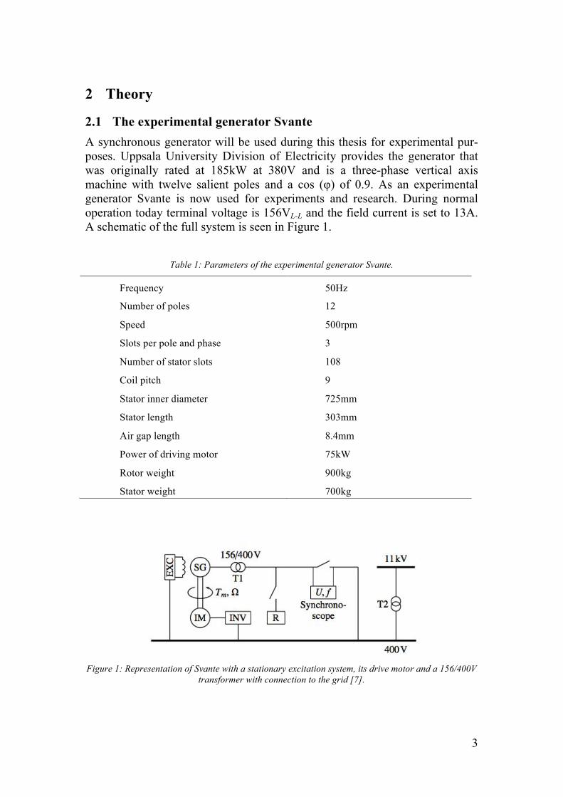
2.1 The experimental generator Svante A synchronous generator will be used during this thesis for experimental pur-poses. Uppsala University Division of Electricity provides the generator that was originally rated at 185kW at 380V and is a three-phase vertical axis machine with twelve salient poles and a cos (φ) of 0.9. As an experimental generator Svante is now used for experiments and research. During normal operation today terminal voltage is 156VL-L and the field current is set to 13A. A schematic of the full system is seen in Figure 1.

Table 1: Parameters of the experimental generator Svante.

Frequency 50Hz

Number of poles 12

Speed 500rpm

Slots per pole and phase 3

Number of stator slots 108

Coil pitch 9

Stator inner diameter 725mm

Stator length 303mm

Air gap length 8.4mm

Power of driving motor 75kW

Rotor weight 900kg

Stator weight 700kg

Figure 1: Representation of Svante with a stationary excitation system, its drive motor and a 156/400V

transformer with connection to the grid [7].

4

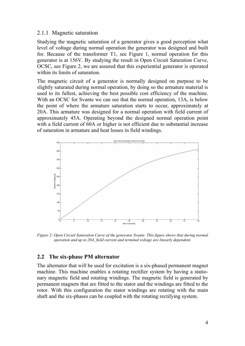
2.1.1 Magnetic saturation Studying the magnetic saturation of a generator gives a good perception what level of voltage during normal operation the generator was designed and built for. Because of the transformer T1, see Figure 1, normal operation for this generator is at 156V. By studying the result in Open Circuit Saturation Curve, OCSC, see Figure 2, we are assured that this experiential generator is operated within its limits of saturation. The magnetic circuit of a generator is normally designed on purpose to be slightly saturated during normal operation, by doing so the armature material is used to its fullest, achieving the best possible cost efficiency of the machine. With an OCSC for Svante we can see that the normal operation, 13A, is below the point of where the armature saturation starts to occur, approximately at 20A. This armature was designed for a normal operation with field current of approximately 45A. Operating beyond the designed normal operation point with a field current of 60A or higher is not efficient due to substantial increase of saturation in armature and heat losses in field windings.

Figure 2: Open Circuit Saturation Curve of the generator Svante. This figure shows that during normal

operation and up to 20A, field current and terminal voltage are linearly dependent.

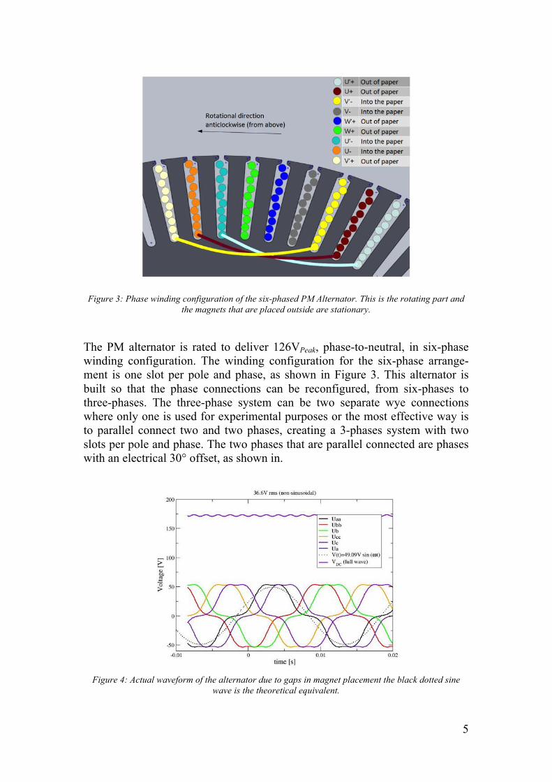
2.2 The six-phase PM alternator The alternator that will be used for excitation is a six-phased permanent magnet machine. This machine enables a rotating rectifier system by having a statio-nary magnetic field and rotating windings. The magnetic field is generated by permanent magnets that are fitted to the stator and the windings are fitted to the rotor. With this configuration the stator windings are rotating with the main shaft and the six-phases can be coupled with the rotating rectifying system.

5

Figure 3: Phase winding configuration of the six-phased PM Alternator. This is the rotating part and

the magnets that are placed outside are stationary.

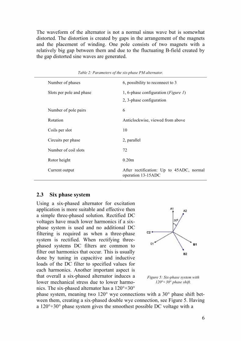
The PM alternator is rated to deliver 126VPeak, phase-to-neutral, in six-phase winding configuration. The winding configuration for the six-phase arrange-ment is one slot per pole and phase, as shown in Figure 3. This alternator is built so that the phase connections can be reconfigured, from six-phases to three-phases. The three-phase system can be two separate wye connections where only one is used for experimental purposes or the most effective way is to parallel connect two and two phases, creating a 3-phases system with two slots per pole and phase. The two phases that are parallel connected are phases with an electrical 30° offset, as shown in.

Figure 4: Actual waveform of the alternator due to gaps in magnet placement the black dotted sine

wave is the theoretical equivalent.

6

The waveform of the alternator is not a normal sinus wave but is somewhat distorted. The distortion is created by gaps in the arrangement of the magnets and the placement of winding. One pole consists of two magnets with a relatively big gap between them and due to the fluctuating B-field created by the gap distorted sine waves are generated.

Table 2: Parameters of the six-phase PM alternator.

Number of phases 6, possibility to reconnect to 3

Slots per pole and phase 1, 6-phase configuration (Figure 1)

2, 3-phase configuration

Number of pole pairs 6

Rotation Anticlockwise, viewed from above

Coils per slot 10

Circuits per phase 2, parallel

Number of coil slots 72

Rotor height 0.20m

Current output After rectification: Up to 45ADC, normal operation 13-15ADC

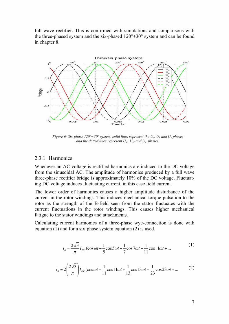
2.3 Six phase system Using a six-phased alternator for excitation application is more suitable and effective then a simple three-phased solution. Rectified DC voltages have much lower harmonics if a six-phase system is used and no additional DC filtering is required as when a three-phase system is rectified. When rectifying three-phased systems DC filters are common to filter out harmonics that occur. This is usually done by tuning in capacitive and inductive loads of the DC filter to specified values for each harmonics. Another important aspect is that overall a six-phased alternator induces a lower mechanical stress due to lower harmo-nics. The six-phased alternator has a 120°+30° phase system, meaning two 120° wye connections with a 30° phase shift bet-ween them, creating a six-phased double wye connection, see Figure 5. Having a 120°+30° phase system gives the smoothest possible DC voltage with a

Figure 5: Six-phase system with 120°+30° phase shift.

7

full wave rectifier. This is confirmed with simulations and comparisons with the three-phased system and the six-phased 120°+30° system and can be found in chapter 8.

2.3.1 Harmonics Whenever an AC voltage is rectified harmonics are induced to the DC voltage from the sinusoidal AC. The amplitude of harmonics produced by a full wave three-phase rectifier bridge is approximately 10% of the DC voltage. Fluctuat-ing DC voltage induces fluctuating current, in this case field current. The lower order of harmonics causes a higher amplitude disturbance of the current in the rotor windings. This induces mechanical torque pulsation to the rotor as the strength of the B-field seen from the stator fluctuates with the current fluctuations in the rotor windings. This causes higher mechanical fatigue to the stator windings and attachments. Calculating current harmonics of a three-phase wye-connection is done with equation (1) and for a six-phase system equation (2) is used.

(1)

(2)

Figure 6: Six-phase 120°+30° system, solid lines represent the Ua, Ub and Uc phases and the dotted lines represent Ua’, Ub’ and Uc’ phases.

iA =2 3π

IDC (cosωt −15cos5ωt + 1

7cos7ωt − 1

11cos11ωt +...

iA = 22 3π

!

"#

$

%&IDC (cosωt −

111cos11ωt + 1

13cos13ωt − 1

23cos23ωt +...

8

Equation (2) shows that the six-phased system holds a higher order of har-monics, 12k±1, while a simple three-phase wye system holds a lower order of harmo-nics, 6k±1, as shown in equation (1). The result is that a lower mechanical stress is induced with a six-phase system. Reduction of the harmonics for a three-phased system can be accomplished by modifying the rectifier system. The six-pulse system is swapped with a 12-pulse system. And by using a wye-wye and a wye-delta transformer as shown in Figure 7, the same effect is achieved regarding the harmonics. Wye-delta transformer shifts the three phases 30° and the 120°+30° phased system is realized.

2.4 Voltage regulation Voltage control and grid stability issues are related to weak systems and long transmissions lines. But these kinds of problems are also linked to the constantly increasing demands for electricity, even in strong and highly deve-loped countries where the power suppliers cannot keep up with the constantly increasing demands for electricity. AVR is a feedback system that is constantly monitoring the produced voltage level at the generator terminals and with a controller the AVR system is able to regulate the excitation level of the rotor. Terminal voltage, UL-L, magnetic field of the rotor poles the (B-field), B, and the field current, If are directly proportional. By controlling the excitation of the rotor poles proportional control of the amplitude of terminal voltage is achieved as shown in equation (3).

(3)

Generator formula shows the direct relationship of the magnetic field, B, and terminal voltage, UL-L. The other variables are fr which is a product of distribution factor, kd, and the pitch factor, kp, p is the number of poles, q is the

UL−L =32fr2pqBδ

0lsωmRr

Figure 7: Three-phase system with wye-wye and wye-delta transformers creating a 120°+30° six-phase system. This is a common solution to the harmonic problem linked to

torque pulsation caused by three-phase excitation systems.

9

number of slots per pole and phase, ls is the stator length, ωm is the angular frequency of the rotor and Rr is the rotor radius. A desired level of UL-L is set to the controller and depending on the desired dynamics of the system P-, PD-, PI- or PID-controller is used and its Kp, Ki and Kd values can be determined [2].

2.4.1 Ziegler–Nichols method Ziegler-Nichols method is a commonly used method in industries to give a first estimate of the parameters of a P-, PD-, PI- and PID-controller for different processes. With this method good and stable baseline values are calculated for the controller. Kp, Ki and Kd can of course later be fine tuned so that the properties meet specific requirements for the controller [13] [14]. The Method:

1. Run the process under normal operation with the controller system active.

2. Choose the P-controller 3. The Kp value is increased from zero until the output signal y starts to

oscillate with constant amplitude. That Kp value is called the ultimate sensitivity, Su.

4. The period of the constant oscillating output signal is called the ultimate period, Pu.

5. Now that all necessary measurements are found and Kp, Ki and Kd can be calculated using Table 3, if there is any stability issue the Kp value needs to be decreased.

Table 3: Ziegler-Nichols method calculation table is used to calculate KP, KI and KD values.

Type Kp Ki Kd

P Su/2 - -

PI Su/2.2 1.2Kp/Pu -

PID 0.60Su 2Kp/Pu KpPu/8

Pessen Integral Rule 0.7Su 2.5Kp/Pu 0.15KpPu

Some Overshoot 0.33Su 2Kp/Pu KpPu/3

No Overshoot 0.2Su 2Kp/Pu KpPu/3

10

2.5 Excitation systems An excitation system provides DC current that is conducted thru the field windings. There are many variations of excitation systems in use. Mostly used today are AC powered, either by an alternator mounted on the main shaft with a rotating rectifying bridge, or by drawing AC power from the grid rectifying stationary and then conducting DC power to the rotor by slip rings and brushes.

Table 4: Example of excitation systems that are common in industry today.

Category Type Power source Used

DC Commutator, Brushless

(Rotating)

Generator main shaft

Outdated

AC AC/DC, Slip rings

(Static rectifier)

3-phase AC, Grid

Mainly used today

AC Alternator, Brushless

(Rotating rectifier)

Generator main Shaft

Recent

With a rotating excitation system there is a lower resistance throughout the excitation system. DC power is directly conducted to the rotor without slip rings and brushes as shown in Figure 20. By measuring resistance at no-load in Svante’s rotor windings, the slip rings and the cables, the resistive difference between a rotating and a stationary excitation system can be calculated [8]. Comparing resistance, stationary and a rotating excitation system:

• Rotor windings, slip rings and cables (red and blue): 3.367 Ω

• Total resistance in all pole windings: 3.03 Ω The result is ≈10% less resistance when exciting directly without use of slip rings and relatively long transferring cables approximately 10m long.

11

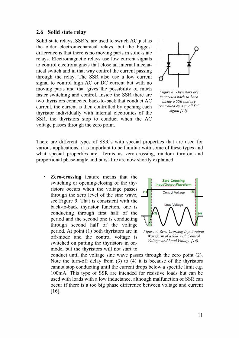
2.6 Solid state relay Solid-state relays, SSR’s, are used to switch AC just as the older electromechanical relays, but the biggest difference is that there is no moving parts in solid-state relays. Electromagnetic relays use low current signals to control electromagnets that close an internal mecha-nical switch and in that way control the current passing through the relay. The SSR also use a low current signal to control high AC or DC current but with no moving parts and that gives the possibility of much faster switching and control. Inside the SSR there are two thyristors connected back-to-back that conduct AC current, the current is then controlled by opening each thyristor individually with internal electronics of the SSR, the thyristors stop to conduct when the AC voltage passes through the zero point. There are different types of SSR’s with special properties that are used for various applications, it is important to be familiar with some of these types and what special properties are. Terms as zero-crossing, random turn-on and proportional phase-angle and burst-fire are now shortly explained.

• Zero-crossing feature means that the switching or opening/closing of the thy-ristors occurs when the voltage passes through the zero level of the sine wave, see Figure 9. That is consistent with the back-to-back thyristor function, one is conducting through first half of the period and the second one is conducting through second half of the voltage period. At point (1) both thyristors are in off-mode and the control voltage is switched on putting the thyristors in on-mode, but the thyristors will not start to conduct until the voltage sine wave passes through the zero point (2). Note the turn-off delay from (3) to (4) it is because of the thyristors cannot stop conducting until the current drops below a specific limit e.g. 100mA. This type of SSR are intended for resistive loads but can be used with loads with a low inductance, although malfunction of SSR can occur if there is a too big phase difference between voltage and current [16].

Figure 8: Thyristors are connected back-to-back

inside a SSR and are controlled by a small DC

signal [15].

Figure 9: Zero-Crossing Input/output Waveform of a SSR with Control Voltage and Load Voltage [16].

12

• Random Turn-on means that the SSR can turn on the AC voltage instantly at any point, switching time is about 100µs or less. Figure 10 shows that there is no delay between point (1) and (2) and the same thyristor turn-off delay as mentioned earlier. These kinds of SSR’s are suited for controlling the AC power for inductive loads with power factor of <0.75, there are no issues with phase difference between voltage and current [16].

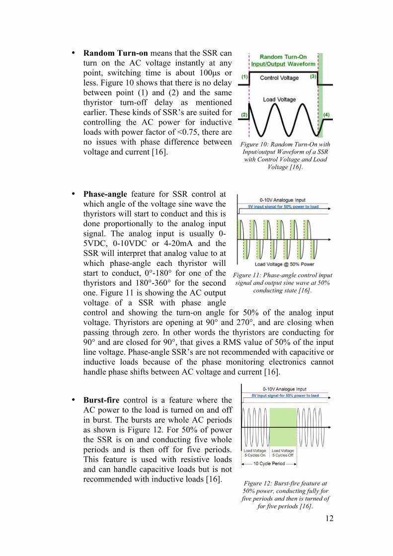
• Phase-angle feature for SSR control at which angle of the voltage sine wave the thyristors will start to conduct and this is done proportionally to the analog input signal. The analog input is usually 0-5VDC, 0-10VDC or 4-20mA and the SSR will interpret that analog value to at which phase-angle each thyristor will start to conduct, 0°-180° for one of the thyristors and 180°-360° for the second one. Figure 11 is showing the AC output voltage of a SSR with phase angle control and showing the turn-on angle for 50% of the analog input voltage. Thyristors are opening at 90° and 270°, and are closing when passing through zero. In other words the thyristors are conducting for 90° and are closed for 90°, that gives a RMS value of 50% of the input line voltage. Phase-angle SSR’s are not recommended with capacitive or inductive loads because of the phase monitoring electronics cannot handle phase shifts between AC voltage and current [16].

• Burst-fire control is a feature where the AC power to the load is turned on and off in burst. The bursts are whole AC periods as shown is Figure 12. For 50% of power the SSR is on and conducting five whole periods and is then off for five periods. This feature is used with resistive loads and can handle capacitive loads but is not recommended with inductive loads [16].

Figure 10: Random Turn-On with Input/output Waveform of a SSR with Control Voltage and Load

Voltage [16].

Figure 11: Phase-angle control input signal and output sine wave at 50%

conducting state [16].

Figure 12: Burst-fire feature at 50% power, conducting fully for five periods and then is turned of

for five periods [16].

13

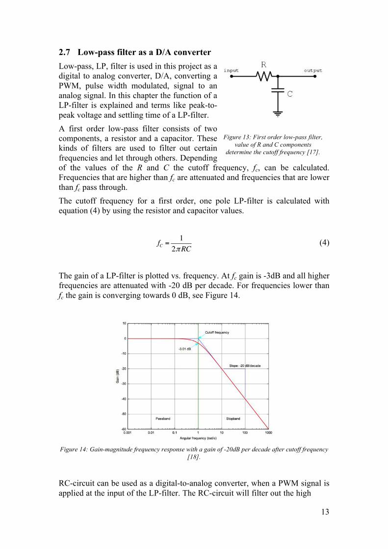
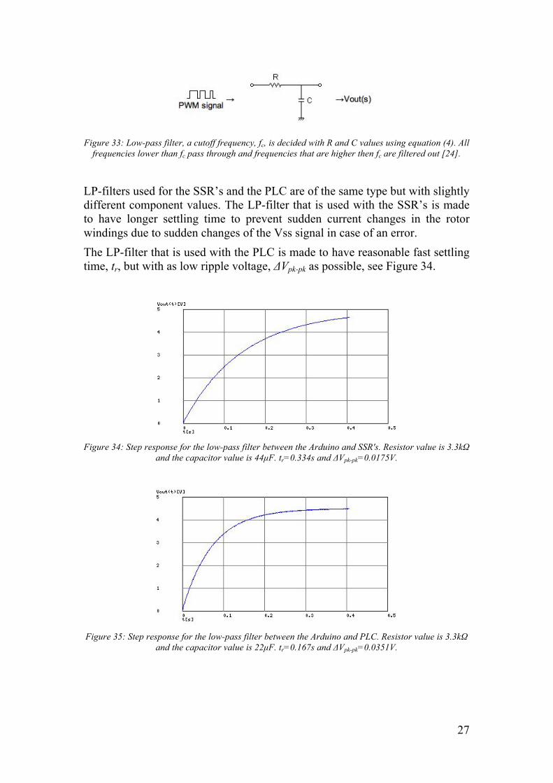
2.7 Low-pass filter as a D/A converter Low-pass, LP, filter is used in this project as a digital to analog converter, D/A, converting a PWM, pulse width modulated, signal to an analog signal. In this chapter the function of a LP-filter is explained and terms like peak-to-peak voltage and settling time of a LP-filter. A first order low-pass filter consists of two components, a resistor and a capacitor. These kinds of filters are used to filter out certain frequencies and let through others. Depending of the values of the R and C the cutoff frequency, fc, can be calculated. Frequencies that are higher than fc are attenuated and frequencies that are lower than fc pass through. The cutoff frequency for a first order, one pole LP-filter is calculated with equation (4) by using the resistor and capacitor values.

fC =1

2πRC (4)

The gain of a LP-filter is plotted vs. frequency. At fc gain is -3dB and all higher frequencies are attenuated with -20 dB per decade. For frequencies lower than fc the gain is converging towards 0 dB, see Figure 14.

Figure 14: Gain-magnitude frequency response with a gain of -20dB per decade after cutoff frequency

[18].

RC-circuit can be used as a digital-to-analog converter, when a PWM signal is applied at the input of the LP-filter. The RC-circuit will filter out the high

Figure 13: First order low-pass filter, value of R and C components

determine the cutoff frequency [17].

14

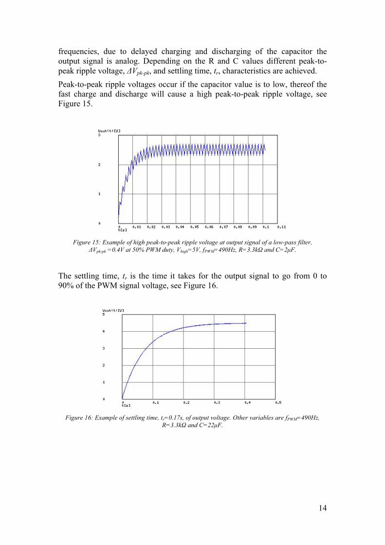
frequencies, due to delayed charging and discharging of the capacitor the output signal is analog. Depending on the R and C values different peak-to-peak ripple voltage, ΔVpk-pk, and settling time, tr, characteristics are achieved. Peak-to-peak ripple voltages occur if the capacitor value is to low, thereof the fast charge and discharge will cause a high peak-to-peak ripple voltage, see Figure 15.

Figure 15: Example of high peak-to-peak ripple voltage at output signal of a low-pass filter,

ΔVpk-pk =0.4V at 50% PWM duty, Vhigh=5V, fPWM=490Hz, R=3.3kΩ and C=2µF.

The settling time, tr is the time it takes for the output signal to go from 0 to 90% of the PWM signal voltage, see Figure 16.

Figure 16: Example of settling time, tr=0.17s, of output voltage. Other variables are fPWM=490Hz,

R=3.3kΩ and C=22µF.

15

3 Method

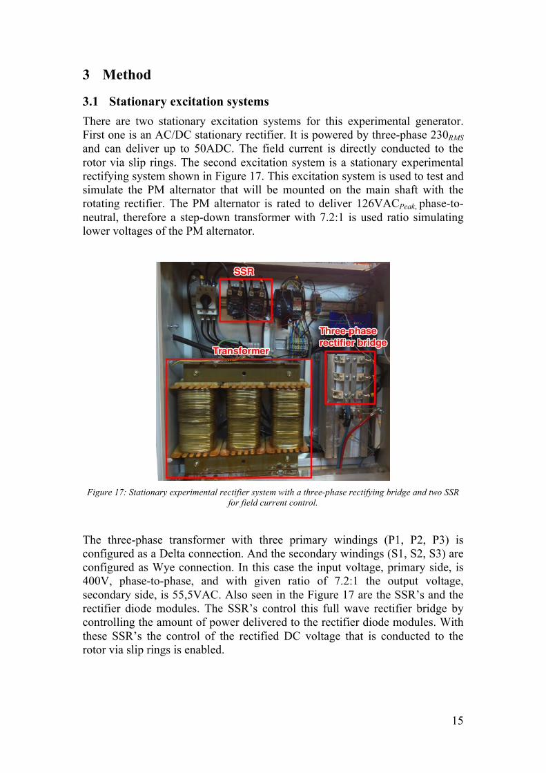
3.1 Stationary excitation systems There are two stationary excitation systems for this experimental generator. First one is an AC/DC stationary rectifier. It is powered by three-phase 230RMS and can deliver up to 50ADC. The field current is directly conducted to the rotor via slip rings. The second excitation system is a stationary experimental rectifying system shown in Figure 17. This excitation system is used to test and simulate the PM alternator that will be mounted on the main shaft with the rotating rectifier. The PM alternator is rated to deliver 126VACPeak, phase-to-neutral, therefore a step-down transformer with 7.2:1 is used ratio simulating lower voltages of the PM alternator.

Figure 17: Stationary experimental rectifier system with a three-phase rectifying bridge and two SSR

for field current control.

The three-phase transformer with three primary windings (P1, P2, P3) is configured as a Delta connection. And the secondary windings (S1, S2, S3) are configured as Wye connection. In this case the input voltage, primary side, is 400V, phase-to-phase, and with given ratio of 7.2:1 the output voltage, secondary side, is 55,5VAC. Also seen in the Figure 17 are the SSR’s and the rectifier diode modules. The SSR’s control this full wave rectifier bridge by controlling the amount of power delivered to the rectifier diode modules. With these SSR’s the control of the rectified DC voltage that is conducted to the rotor via slip rings is enabled.

16

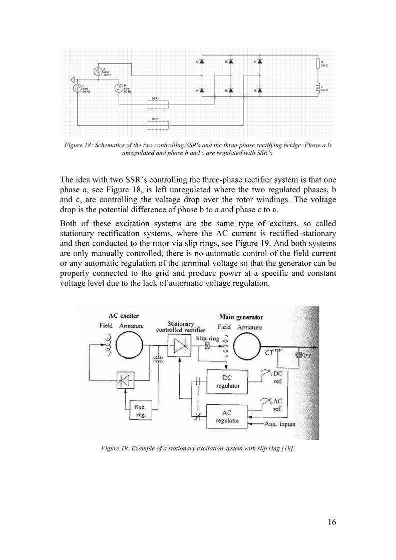
Figure 18: Schematics of the two controlling SSR's and the three-phase rectifying bridge. Phase a is

unregulated and phase b and c are regulated with SSR’s.

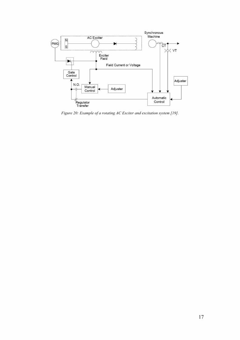
The idea with two SSR’s controlling the three-phase rectifier system is that one phase a, see Figure 18, is left unregulated where the two regulated phases, b and c, are controlling the voltage drop over the rotor windings. The voltage drop is the potential difference of phase b to a and phase c to a. Both of these excitation systems are the same type of exciters, so called stationary rectification systems, where the AC current is rectified stationary and then conducted to the rotor via slip rings, see Figure 19. And both systems are only manually controlled, there is no automatic control of the field current or any automatic regulation of the terminal voltage so that the generator can be properly connected to the grid and produce power at a specific and constant voltage level due to the lack of automatic voltage regulation.

Figure 19: Example of a stationary excitation system with slip ring [19].

17

Figure 20: Example of a rotating AC Exciter and excitation system [19].

18

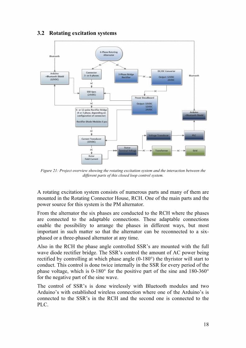
3.2 Rotating excitation systems

Figure 21: Project overview showing the rotating excitation system and the interaction between the

different parts of this closed loop control system.

A rotating excitation system consists of numerous parts and many of them are mounted in the Rotating Connector House, RCH. One of the main parts and the power source for this system is the PM alternator. From the alternator the six phases are conducted to the RCH where the phases are connected to the adaptable connections. These adaptable connections enable the possibility to arrange the phases in different ways, but most important in such matter so that the alternator can be reconnected to a six-phased or a three-phased alternator at any time. Also in the RCH the phase angle controlled SSR’s are mounted with the full wave diode rectifier bridge. The SSR’s control the amount of AC power being rectified by controlling at which phase angle (0-180°) the thyristor will start to conduct. This control is done twice internally in the SSR for every period of the phase voltage, which is 0-180° for the positive part of the sine and 180-360° for the negative part of the sine wave. The control of SSR’s is done wirelessly with Bluetooth modules and two Arduino’s with established wireless connection where one of the Arduino’s is connected to the SSR’s in the RCH and the second one is connected to the PLC.

19

Additionally mounted to the RCH is the power supply system with three voltage supply levels for the Arduino (12VDC), Current Transducer (10VDC) and SSR’s (24VDC). From the RCH the rectified DC current is then conducted directly to the rotor windings allowing rotor excitation. The current transducer is measuring the current that is passing through the rotor windings and is connected to the Arduino so that this information can be sent to the PLC. The terminal voltage is monitored by a voltage transducer that is also con-nected to the PLC creating a closed loop controller system of the excitation. By controlling the excitation of the rotor through e.g. a PI controller with terminal voltage as feedback a closed loop controller is created in the form of a automatic voltage regulator.

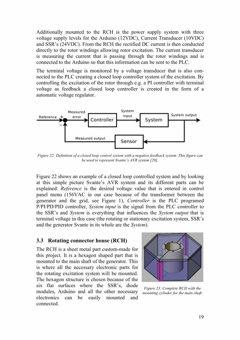
Figure 22: Definition of a closed loop control system with a negative feedback system. This figure can

be used to represent Svante’s AVR system [20].

Figure 22 shows an example of a closed loop controlled system and by looking at this simple picture Svante’s AVR system and its different parts can be explained: Reference is the desired voltage value that is entered in control panel menu (156VAC in our case because of the transformer between the generator and the grid, see Figure 1), Controller is the PLC programed P/PI/PD/PID controller, System input is the signal from the PLC controller to the SSR’s and System is everything that influences the System output that is terminal voltage in this case (the rotating or stationary excitation system, SSR’s and the generator Svante in its whole are the System).

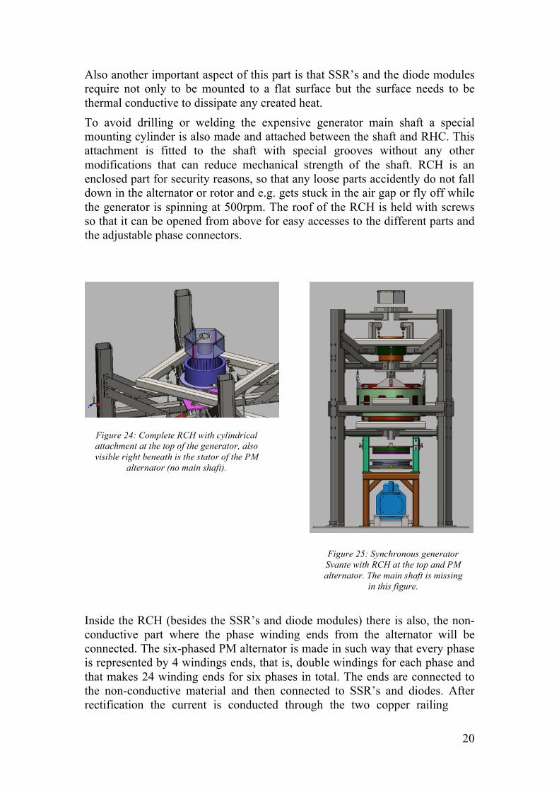
3.3 Rotating connector house (RCH) The RCH is a sheet metal part custom-made for this project. It is a hexagon shaped part that is mounted to the main shaft of the generator. This is where all the necessary electronic parts for the rotating excitation system will be mounted. The hexagon structure is chosen because of the six flat surfaces where the SSR’s, diode modules, Arduino and all the other necessary electronics can be easily mounted and connected.

Figure 23: Complete RCH with the mounting cylinder for the main shaft.

20

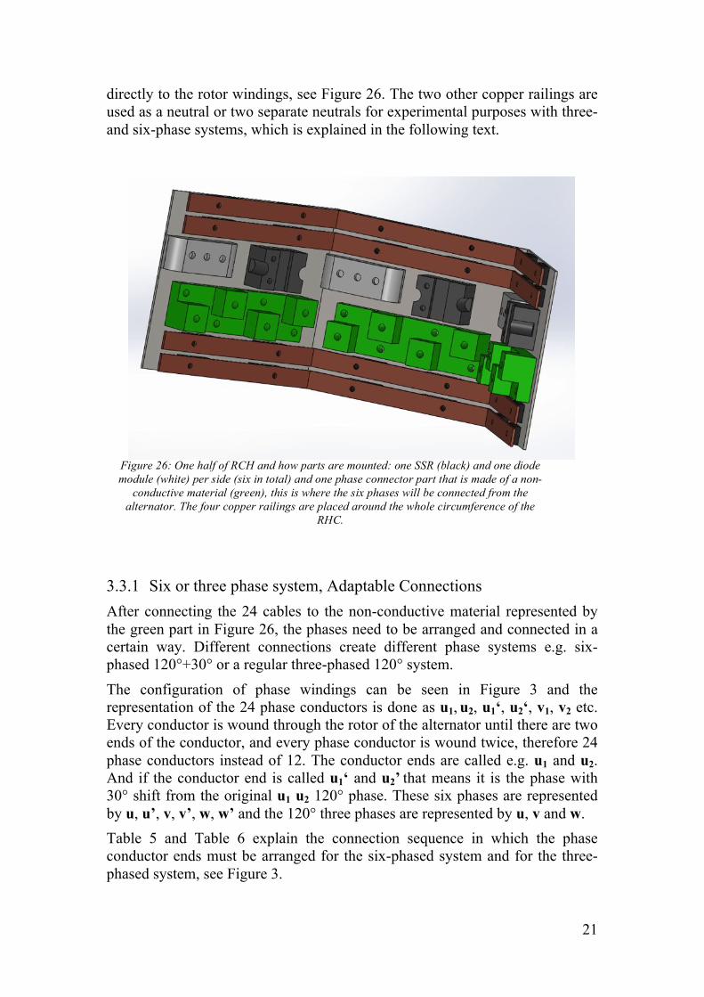
Also another important aspect of this part is that SSR’s and the diode modules require not only to be mounted to a flat surface but the surface needs to be thermal conductive to dissipate any created heat. To avoid drilling or welding the expensive generator main shaft a special mounting cylinder is also made and attached between the shaft and RHC. This attachment is fitted to the shaft with special grooves without any other modifications that can reduce mechanical strength of the shaft. RCH is an enclosed part for security reasons, so that any loose parts accidently do not fall down in the alternator or rotor and e.g. gets stuck in the air gap or fly off while the generator is spinning at 500rpm. The roof of the RCH is held with screws so that it can be opened from above for easy accesses to the different parts and the adjustable phase connectors.

Inside the RCH (besides the SSR’s and diode modules) there is also, the non-conductive part where the phase winding ends from the alternator will be connected. The six-phased PM alternator is made in such way that every phase is represented by 4 windings ends, that is, double windings for each phase and that makes 24 winding ends for six phases in total. The ends are connected to the non-conductive material and then connected to SSR’s and diodes. After rectification the current is conducted through the two copper railing

Figure 25: Synchronous generator Svante with RCH at the top and PM alternator. The main shaft is missing

in this figure.

Figure 24: Complete RCH with cylindrical attachment at the top of the generator, also visible right beneath is the stator of the PM

alternator (no main shaft).

21

directly to the rotor windings, see Figure 26. The two other copper railings are used as a neutral or two separate neutrals for experimental purposes with three- and six-phase systems, which is explained in the following text.

3.3.1 Six or three phase system, Adaptable Connections After connecting the 24 cables to the non-conductive material represented by the green part in Figure 26, the phases need to be arranged and connected in a certain way. Different connections create different phase systems e.g. six-phased 120°+30° or a regular three-phased 120° system. The configuration of phase windings can be seen in Figure 3 and the representation of the 24 phase conductors is done as u1, u2, u1‘, u2‘, v1, v2 etc. Every conductor is wound through the rotor of the alternator until there are two ends of the conductor, and every phase conductor is wound twice, therefore 24 phase conductors instead of 12. The conductor ends are called e.g. u1 and u2. And if the conductor end is called u1‘ and u2’ that means it is the phase with 30° shift from the original u1 u2 120° phase. These six phases are represented by u, u’, v, v’, w, w’ and the 120° three phases are represented by u, v and w. Table 5 and Table 6 explain the connection sequence in which the phase conductor ends must be arranged for the six-phased system and for the three-phased system, see Figure 3.

Figure 26: One half of RCH and how parts are mounted: one SSR (black) and one diode module (white) per side (six in total) and one phase connector part that is made of a non-

conductive material (green), this is where the six phases will be connected from the alternator. The four copper railings are placed around the whole circumference of the

RHC.

22

Table 5: Connection arrangement for a six-phased alternator system.

u21-u12 U

u21’-u12’ U’

v21-v12 V

v21’-v12’ V’

w21-w12 W

w21’-w12’ W’

u11, u22, v11, v22, w11, w22 N1

u11’, u22’, v11’, v22’, w11’, w22’ N2

Table 6: Connection arrangement for a three-phased alternator system.

u21-u21’ U

v21-v11 -

v21’-v11’ -

w21-w21’ W

u12-u22 -

u12’-u22’ -

v12-v12’ V

w12-w22 -

w12’-w22’ -

u11, u11’, w11, w11’, v22, v22’ N1

- N2

23

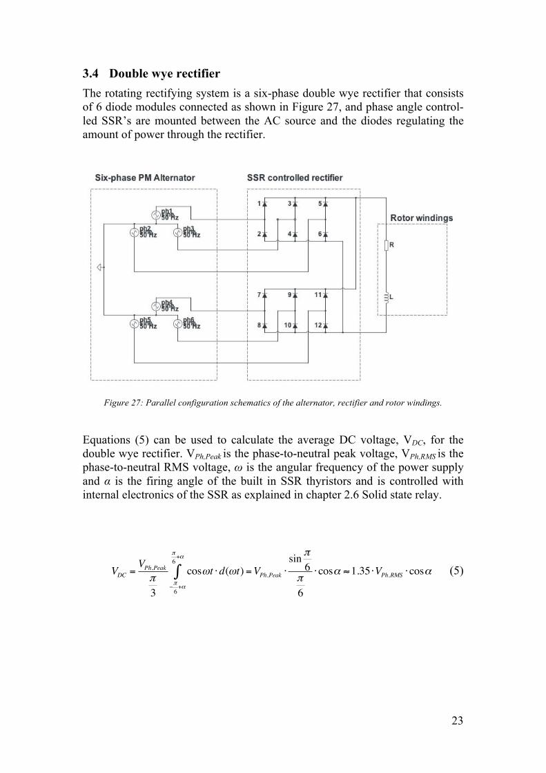
3.4 Double wye rectifier The rotating rectifying system is a six-phase double wye rectifier that consists of 6 diode modules connected as shown in Figure 27, and phase angle control-led SSR’s are mounted between the AC source and the diodes regulating the amount of power through the rectifier.

Figure 27: Parallel configuration schematics of the alternator, rectifier and rotor windings.

Equations (5) can be used to calculate the average DC voltage, VDC, for the double wye rectifier. VPh,Peak is the phase-to-neutral peak voltage, VPh,RMS is the phase-to-neutral RMS voltage, ω is the angular frequency of the power supply and α is the firing angle of the built in SSR thyristors and is controlled with internal electronics of the SSR as explained in chapter 2.6 Solid state relay.

VDC =VPh,Peakπ3

cosωt ⋅d(ωt)−π6+α

π6+α

∫ =VPh,Peak ⋅sin π6

π6

⋅cosα ≈1.35 ⋅VPh,RMS ⋅cosα (5)

24

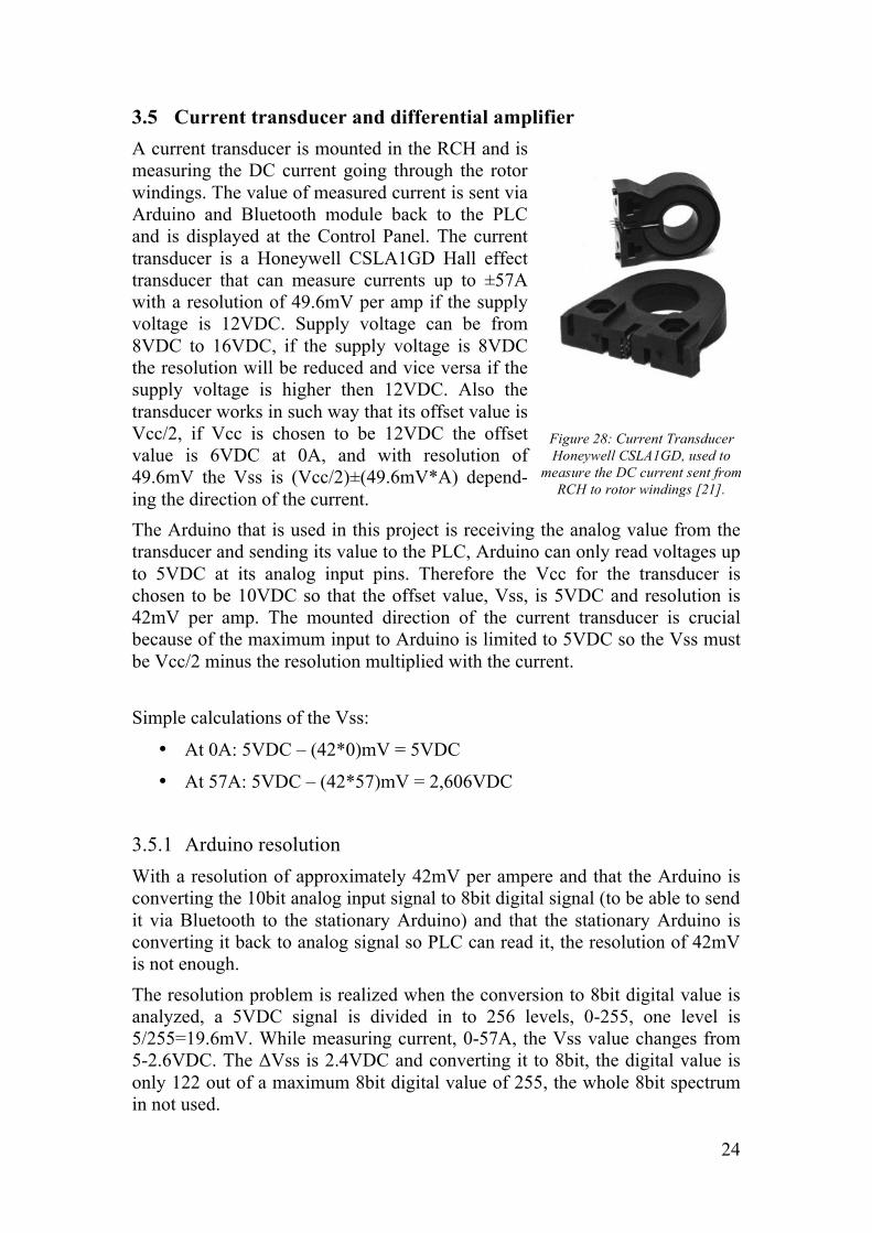
3.5 Current transducer and differential amplifier A current transducer is mounted in the RCH and is measuring the DC current going through the rotor windings. The value of measured current is sent via Arduino and Bluetooth module back to the PLC and is displayed at the Control Panel. The current transducer is a Honeywell CSLA1GD Hall effect transducer that can measure currents up to ±57A with a resolution of 49.6mV per amp if the supply voltage is 12VDC. Supply voltage can be from 8VDC to 16VDC, if the supply voltage is 8VDC the resolution will be reduced and vice versa if the supply voltage is higher then 12VDC. Also the transducer works in such way that its offset value is Vcc/2, if Vcc is chosen to be 12VDC the offset value is 6VDC at 0A, and with resolution of 49.6mV the Vss is (Vcc/2)±(49.6mV*A) depend-ing the direction of the current. The Arduino that is used in this project is receiving the analog value from the transducer and sending its value to the PLC, Arduino can only read voltages up to 5VDC at its analog input pins. Therefore the Vcc for the transducer is chosen to be 10VDC so that the offset value, Vss, is 5VDC and resolution is 42mV per amp. The mounted direction of the current transducer is crucial because of the maximum input to Arduino is limited to 5VDC so the Vss must be Vcc/2 minus the resolution multiplied with the current.

Simple calculations of the Vss:

• At 0A: 5VDC – (42*0)mV = 5VDC

• At 57A: 5VDC – (42*57)mV = 2,606VDC

3.5.1 Arduino resolution With a resolution of approximately 42mV per ampere and that the Arduino is converting the 10bit analog input signal to 8bit digital signal (to be able to send it via Bluetooth to the stationary Arduino) and that the stationary Arduino is converting it back to analog signal so PLC can read it, the resolution of 42mV is not enough. The resolution problem is realized when the conversion to 8bit digital value is analyzed, a 5VDC signal is divided in to 256 levels, 0-255, one level is 5/255=19.6mV. While measuring current, 0-57A, the Vss value changes from 5-2.6VDC. The ΔVss is 2.4VDC and converting it to 8bit, the digital value is only 122 out of a maximum 8bit digital value of 255, the whole 8bit spectrum in not used.

Figure 28: Current Transducer Honeywell CSLA1GD, used to

measure the DC current sent from RCH to rotor windings [21].

25

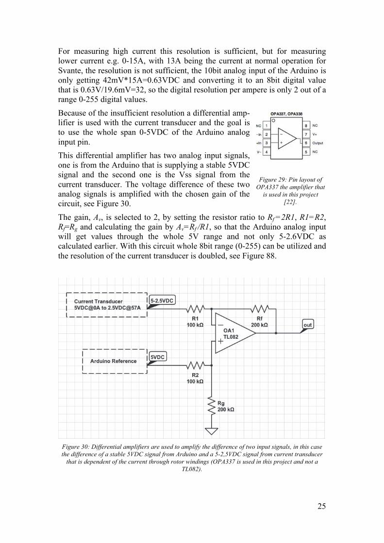
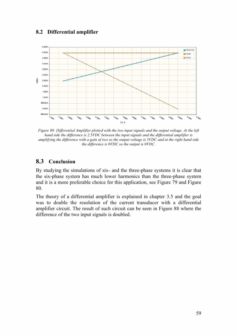
For measuring high current this resolution is sufficient, but for measuring lower current e.g. 0-15A, with 13A being the current at normal operation for Svante, the resolution is not sufficient, the 10bit analog input of the Arduino is only getting 42mV*15A=0.63VDC and converting it to an 8bit digital value that is 0.63V/19.6mV=32, so the digital resolution per ampere is only 2 out of a range 0-255 digital values. Because of the insufficient resolution a differential amp-lifier is used with the current transducer and the goal is to use the whole span 0-5VDC of the Arduino analog input pin. This differential amplifier has two analog input signals, one is from the Arduino that is supplying a stable 5VDC signal and the second one is the Vss signal from the current transducer. The voltage difference of these two analog signals is amplified with the chosen gain of the circuit, see Figure 30. The gain, Av, is selected to 2, by setting the resistor ratio to Rf =2R1, R1=R2, Rf=Rg and calculating the gain by Av=Rf /R1, so that the Arduino analog input will get values through the whole 5V range and not only 5-2.6VDC as calculated earlier. With this circuit whole 8bit range (0-255) can be utilized and the resolution of the current transducer is doubled, see Figure 88.

Figure 30: Differential amplifiers are used to amplify the difference of two input signals, in this case the difference of a stable 5VDC signal from Arduino and a 5-2,5VDC signal from current transducer

that is dependent of the current through rotor windings (OPA337 is used in this project and not a TL082).

Figure 29: Pin layout of OPA337 the amplifier that

is used in this project [22].

26

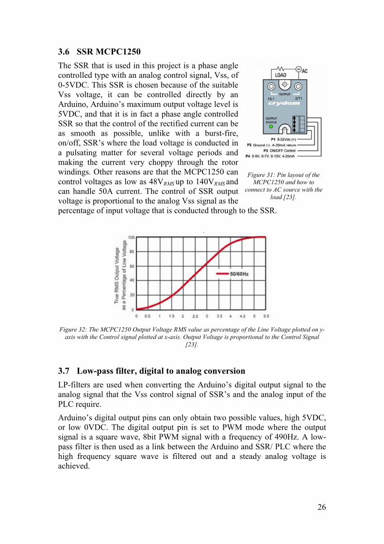
3.6 SSR MCPC1250 The SSR that is used in this project is a phase angle controlled type with an analog control signal, Vss, of 0-5VDC. This SSR is chosen because of the suitable Vss voltage, it can be controlled directly by an Arduino, Arduino’s maximum output voltage level is 5VDC, and that it is in fact a phase angle controlled SSR so that the control of the rectified current can be as smooth as possible, unlike with a burst-fire, on/off, SSR’s where the load voltage is conducted in a pulsating matter for several voltage periods and making the current very choppy through the rotor windings. Other reasons are that the MCPC1250 can control voltages as low as 48VRMS up to 140VRMS and can handle 50A current. The control of SSR output voltage is proportional to the analog Vss signal as the percentage of input voltage that is conducted through to the SSR.

Figure 32: The MCPC1250 Output Voltage RMS value as percentage of the Line Voltage plotted on y-

axis with the Control signal plotted at x-axis. Output Voltage is proportional to the Control Signal [23].

3.7 Low-pass filter, digital to analog conversion LP-filters are used when converting the Arduino’s digital output signal to the analog signal that the Vss control signal of SSR’s and the analog input of the PLC require. Arduino’s digital output pins can only obtain two possible values, high 5VDC, or low 0VDC. The digital output pin is set to PWM mode where the output signal is a square wave, 8bit PWM signal with a frequency of 490Hz. A low-pass filter is then used as a link between the Arduino and SSR/ PLC where the high frequency square wave is filtered out and a steady analog voltage is achieved.

Figure 31: Pin layout of the MCPC1250 and how to

connect to AC source with the load [23].

27

Figure 33: Low-pass filter, a cutoff frequency, fc, is decided with R and C values using equation (4). All

frequencies lower than fc pass through and frequencies that are higher then fc are filtered out [24].

LP-filters used for the SSR’s and the PLC are of the same type but with slightly different component values. The LP-filter that is used with the SSR’s is made to have longer settling time to prevent sudden current changes in the rotor windings due to sudden changes of the Vss signal in case of an error. The LP-filter that is used with the PLC is made to have reasonable fast settling time, tr, but with as low ripple voltage, ΔVpk-pk as possible, see Figure 34.

Figure 34: Step response for the low-pass filter between the Arduino and SSR's. Resistor value is 3.3kΩ

and the capacitor value is 44µF. tr=0.334s and ΔVpk-pk=0.0175V.

Figure 35: Step response for the low-pass filter between the Arduino and PLC. Resistor value is 3.3kΩ

and the capacitor value is 22µF. tr=0.167s and ΔVpk-pk=0.0351V.

28

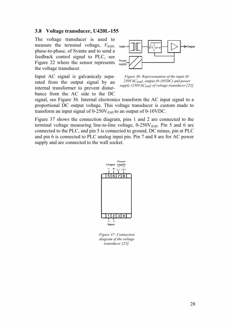
3.8 Voltage transducer, U420L-155 The voltage transducer is used to measure the terminal voltage, VRMS, phase-to-phase, of Svante and to send a feedback control signal to PLC, see Figure 22 where the sensor represents the voltage transducer. Input AC signal is galvanicaly sepa-rated from the output signal by an internal transformer to prevent distur-bance from the AC side to the DC signal, see Figure 36. Internal electronics transform the AC input signal to a proportional DC output voltage. This voltage transducer is custom made to transform an input signal of 0-250VRMS to an output of 0-10VDC. Figure 37 shows the connection diagram, pins 1 and 2 are connected to the terminal voltage measuring line-to-line voltage, 0-250VRMS. Pin 5 and 6 are connected to the PLC, and pin 5 is connected to ground, DC minus, pin at PLC and pin 6 is connected to PLC analog input pin. Pin 7 and 8 are for AC power supply and are connected to the wall socket.

Figure 36: Representation of the input (0-250VACRMS), output (0-10VDC) and power

supply (230VACRMS) of voltage transducer [25].

Figure 37: Connection diagram of the voltage

transducer [25].

29

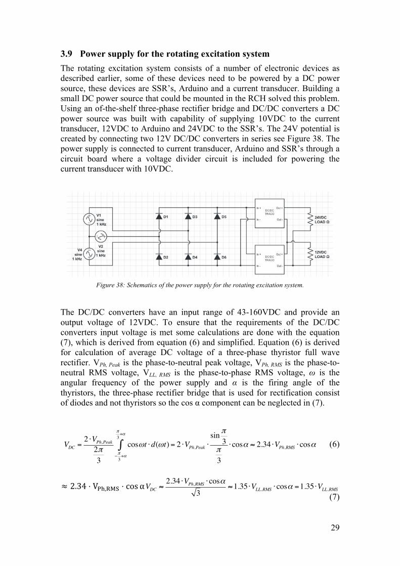
3.9 Power supply for the rotating excitation system The rotating excitation system consists of a number of electronic devices as described earlier, some of these devices need to be powered by a DC power source, these devices are SSR’s, Arduino and a current transducer. Building a small DC power source that could be mounted in the RCH solved this problem. Using an of-the-shelf three-phase rectifier bridge and DC/DC converters a DC power source was built with capability of supplying 10VDC to the current transducer, 12VDC to Arduino and 24VDC to the SSR’s. The 24V potential is created by connecting two 12V DC/DC converters in series see Figure 38. The power supply is connected to current transducer, Arduino and SSR’s through a circuit board where a voltage divider circuit is included for powering the current transducer with 10VDC.

Figure 38: Schematics of the power supply for the rotating excitation system.

The DC/DC converters have an input range of 43-160VDC and provide an output voltage of 12VDC. To ensure that the requirements of the DC/DC converters input voltage is met some calculations are done with the equation (7), which is derived from equation (6) and simplified. Equation (6) is derived for calculation of average DC voltage of a three-phase thyristor full wave rectifier. VPh, Peak is the phase-to-neutral peak voltage, VPh, RMS is the phase-to-neutral RMS voltage, VLL, RMS is the phase-to-phase RMS voltage, ω is the angular frequency of the power supply and α is the firing angle of the thyristors, the three-phase rectifier bridge that is used for rectification consist of diodes and not thyristors so the cos α component can be neglected in (7).

VDC =2 ⋅VPh,Peak2π3

cosωt−π3+α

π3+α

∫ ⋅d(ωt) = 2 ⋅VPh,Peak ⋅sin π

3π3

⋅cosα ≈ 2.34 ⋅VPh,RMS ⋅cosα (6)

≈ 2.34 ⋅ V!",!"# ⋅ cosαVDC ≈2.34 ⋅VPh,RMS ⋅cosα

3≈1.35 ⋅VLL,RMS ⋅cosα =1.35 ⋅VLL,RMS

(7)

30

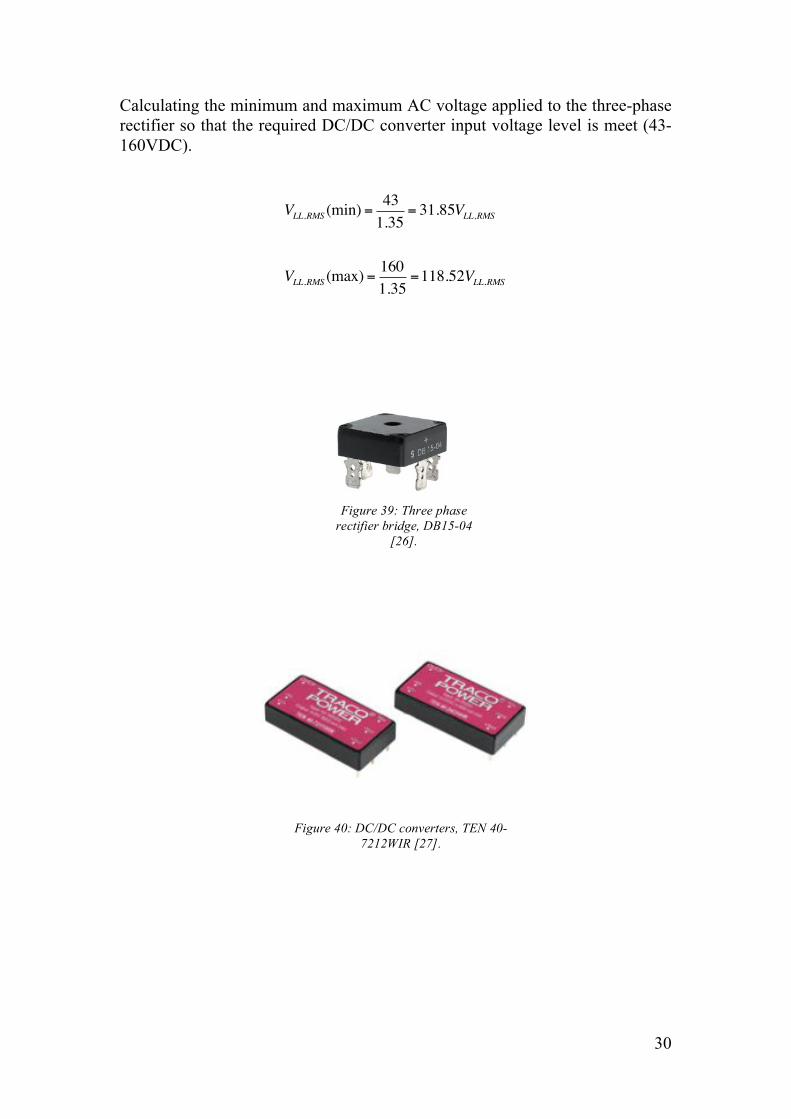
Calculating the minimum and maximum AC voltage applied to the three-phase rectifier so that the required DC/DC converter input voltage level is meet (43-160VDC).

VLL,RMS (min) =431.35

= 31.85VLL,RMS

VLL,RMS (max) =1601.35

=118.52VLL,RMS

Figure 39: Three phase rectifier bridge, DB15-04

[26].

Figure 40: DC/DC converters, TEN 40-7212WIR [27].

31

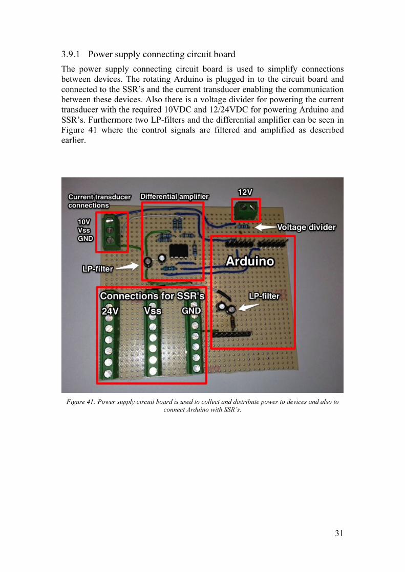
3.9.1 Power supply connecting circuit board The power supply connecting circuit board is used to simplify connections between devices. The rotating Arduino is plugged in to the circuit board and connected to the SSR’s and the current transducer enabling the communication between these devices. Also there is a voltage divider for powering the current transducer with the required 10VDC and 12/24VDC for powering Arduino and SSR’s. Furthermore two LP-filters and the differential amplifier can be seen in Figure 41 where the control signals are filtered and amplified as described earlier.

Figure 41: Power supply circuit board is used to collect and distribute power to devices and also to

connect Arduino with SSR’s.

32

4 PLC

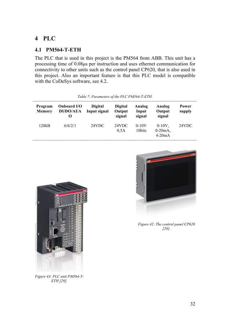
4.1 PM564-T-ETH The PLC that is used in this project is the PM564 from ABB. This unit has a processing time of 0.08µs per instruction and uses ethernet communication for connectivity to other units such as the control panel CP620, that is also used in this project. Also an important feature is that this PLC model is compatible with the CoDeSys software, see 4.2.

Table 7: Parameters of the PLC PM564-T-ETH.

Program Memory

Onboard I/O DI/DO/AI/A

O

Digital Input signal

Digital Output signal

Analog Input signal

Analog Output signal

Power supply

128kB 6/6/2/1 24VDC 24VDC 0,5A

0-10V 10bits

0-10V, 0-20mA, 4-20mA

24VDC

Figure 43: PLC unit PM564-T-ETH [29].

Figure 42: The control panel CP620 [28].

33

4.2 Software The developing environment for programing PLC’s is called CoDeSys, Controller Developing System. This software is free and it follows an international standard, IEC 61131-3, for PLC programing, except for the CFC language that is also available in CoDeSys [30]. CoDeSys provides six different programing languages that can be combined and used together to create one program [11]. The languages are:

• IL (Instruction List), resembles assembler programing.

• ST (Structured Text), resembles C programing, see BluetoothCheck in chapter 0.

• LD (Ladder Diagram), graphical programing with virtual e.g. coils and contacts.

• FBD (Function Block Diagram), graphical programing with function blocks e.g. AND & OR gates, see Mode in chapter 0.

• SFC (Sequential Function Chart), graphical programing to simplify making of sequential process, see Mode_Sequence in chapter 0.

• CFC (Continuous Function Chart), graphical programing that is almost like FBD but elements are freely peaceable which allows e.g. feedback, see PLC_PRG in chapter 0.

4.3 Functions block Function blocks, FB, is a Program Organization Unit, POU, that can be found in FBD and CFC languages. The FB is a virtual block with inputs and outputs see Figure 45. Besides the built-in FB that can be used such as e.g. logic gates, custom FB can also be made for specific function [10]. The built-in function blocks that are used in the PLC_PRG, main PLC program, are explained in the following text and in the next chapter 4.4 and also a custom FB is explained in 4.4.1.

Figure 45: Custom made FB Mode and two built-in FB logical OR gates.

Figure 44: CoDeSys logo [30].

34

PLC_PRG:

• TP - Timer

• OR - Logic

• TRUNC - Converter SD_Save_Read

• SD_READ - Reading data from the SD Card

• SD_WRITE - Writing data to the SD Card Save_Read_timer

• TP - Timer

• TON - Timer Regulator

• AND - Logic

• ADD - Math

• PD - Regulator

• PID - Regulator

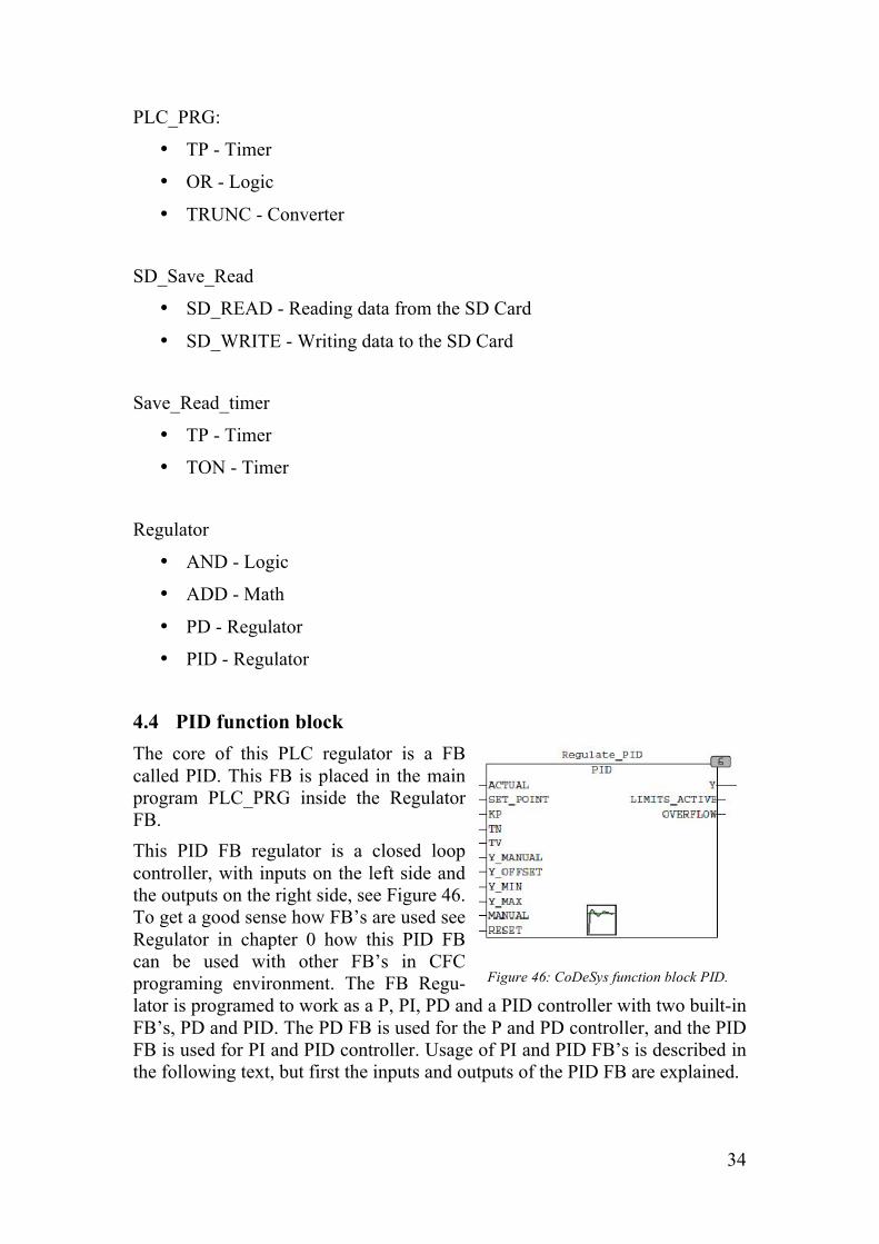
4.4 PID function block The core of this PLC regulator is a FB called PID. This FB is placed in the main program PLC_PRG inside the Regulator FB. This PID FB regulator is a closed loop controller, with inputs on the left side and the outputs on the right side, see Figure 46. To get a good sense how FB’s are used see Regulator in chapter 0 how this PID FB can be used with other FB’s in CFC programing environment. The FB Regu-lator is programed to work as a P, PI, PD and a PID controller with two built-in FB’s, PD and PID. The PD FB is used for the P and PD controller, and the PID FB is used for PI and PID controller. Usage of PI and PID FB’s is described in the following text, but first the inputs and outputs of the PID FB are explained.

Figure 46: CoDeSys function block PID.

35

Inputs and outputs of PID function block [10]:

• ACTUAL is the measured terminal voltage signal.

• SET_POINT is the desired voltage.

• KP is proportional gain.

• TN is integral action time, TN=Kp/Ki.

• TV is derivative action time, TV=Kd/Kp.

• Y_MANUAL defines output value during manual control.

• Y_OFFSET is offset for the output Y.

• Y_MIN is the lower limit for the output Y.

• Y_MAX is the upper limit for the output Y.

• MANUAL determines when manual control is applied.

• RESET resets the controller.

• Y is the calculated output value.

• LIMITS_ACTIVE indicates if Y exceeds minimum or maximum limit.

• OVERFLOW indicates overflow. The PID function block uses equation (8) to calculate the value of Y, where e is the control error, which is the output value subtracted from the desired value (SET_POINT – Y). TN is the integral action time given in milliseconds and the TV variable is the derivative action time also given in milliseconds. The controller FB, PD and PID, use the variable TN and TD instead of Ki and Kd which is more common expression in literature. TN and TD is directed to the industry with the unit being in ms instead of 1/ms. There are also other names for these variables such as Kc, Ti and Td where the units can be min/rep or rep/sec.

Y = KP e(t)+ 1TN

e(τ )dτ +TVddte(t)

0

t

∫"

#$

%

&' (8)

Output Y is directly connected via PLC analog output pin to an Arduino analog input pin that can only handle 5VDC as mentioned earlier. That is why as a safety measurement the lower limit, Y_MIN, is set to 0VDC and the upper limit, Y_MAX, is set to 5VDC for the output Y.

36

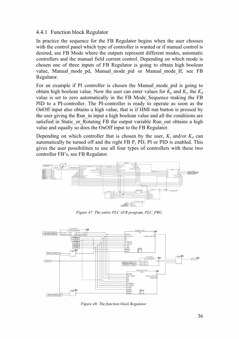
4.4.1 Function block Regulator In practice the sequence for the FB Regulator begins when the user chooses with the control panel which type of controller is wanted or if manual control is desired, see FB Mode where the outputs represent different modes, automatic controllers and the manual field current control. Depending on which mode is chosen one of three inputs of FB Regulator is going to obtain high boolean value, Manual_mode_pd, Manual_mode_pid or Manual_mode_If, see FB Regulator. For an example if PI controller is chosen the Manual_mode_pid is going to obtain high boolean value. Now the user can enter values for Kp and Ki, the Kd value is set to zero automatically in the FB Mode_Sequence making the FB PID to a PI-controller. The PI-controller is ready to operate as soon as the OnOff input also obtains a high value, that is if HMI run button is pressed by the user giving the Run_in input a high boolean value and all the conditions are satisfied in Static_or_Rotating FB the output variable Run_out obtains a high value and equally so does the OnOff input to the FB Regulator. Depending on which controller that is chosen by the user, Ki and/or Kd can automatically be turned off and the right FB P, PD, PI or PID is enabled. This gives the user possibilities to use all four types of controllers with these two controller FB’s, see FB Regulator.

Figure 47: The entire PLC AVR program, PLC_PRG.

Figure 48: The function block Regulator.

37

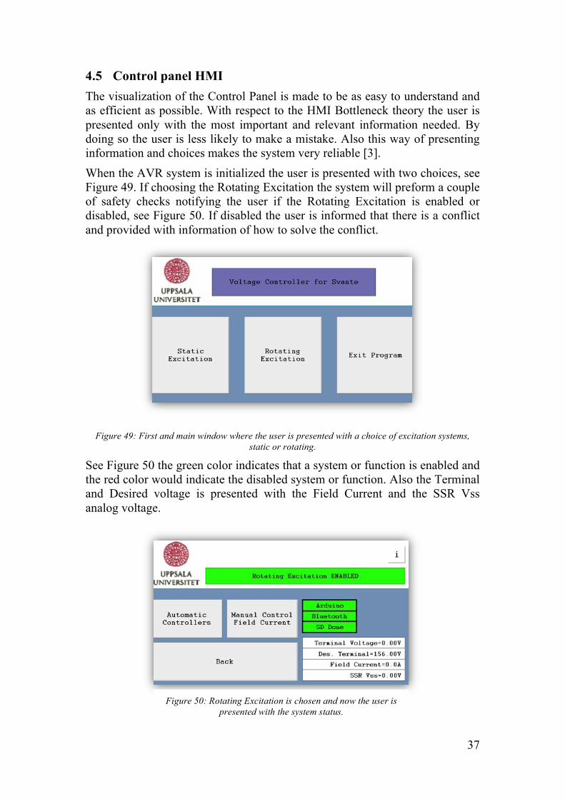
4.5 Control panel HMI The visualization of the Control Panel is made to be as easy to understand and as efficient as possible. With respect to the HMI Bottleneck theory the user is presented only with the most important and relevant information needed. By doing so the user is less likely to make a mistake. Also this way of presenting information and choices makes the system very reliable [3]. When the AVR system is initialized the user is presented with two choices, see Figure 49. If choosing the Rotating Excitation the system will preform a couple of safety checks notifying the user if the Rotating Excitation is enabled or disabled, see Figure 50. If disabled the user is informed that there is a conflict and provided with information of how to solve the conflict.

Figure 49: First and main window where the user is presented with a choice of excitation systems,

static or rotating.

See Figure 50 the green color indicates that a system or function is enabled and the red color would indicate the disabled system or function. Also the Terminal and Desired voltage is presented with the Field Current and the SSR Vss analog voltage.

Figure 50: Rotating Excitation is chosen and now the user is presented with the system status.

38

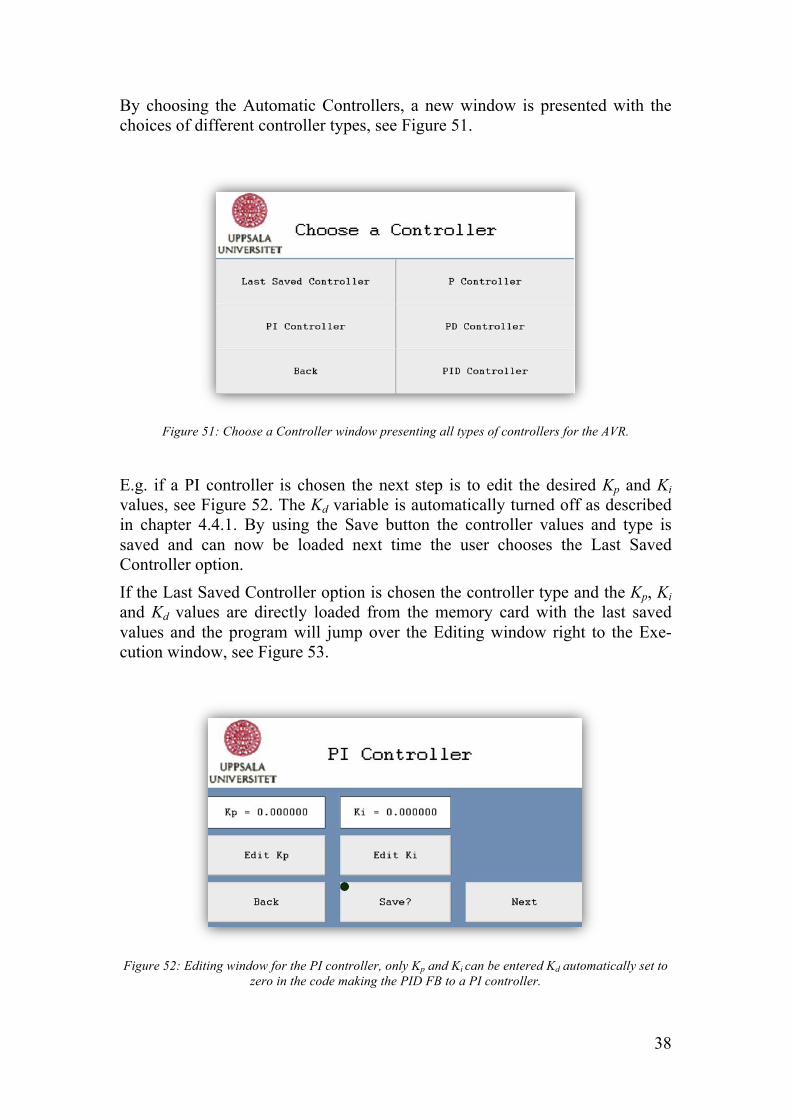
By choosing the Automatic Controllers, a new window is presented with the choices of different controller types, see Figure 51.

Figure 51: Choose a Controller window presenting all types of controllers for the AVR.

E.g. if a PI controller is chosen the next step is to edit the desired Kp and Ki values, see Figure 52. The Kd variable is automatically turned off as described in chapter 4.4.1. By using the Save button the controller values and type is saved and can now be loaded next time the user chooses the Last Saved Controller option. If the Last Saved Controller option is chosen the controller type and the Kp, Ki and Kd values are directly loaded from the memory card with the last saved values and the program will jump over the Editing window right to the Exe-cution window, see Figure 53.

Figure 52: Editing window for the PI controller, only Kp and Ki can be entered Kd automatically set to

zero in the code making the PID FB to a PI controller.

39

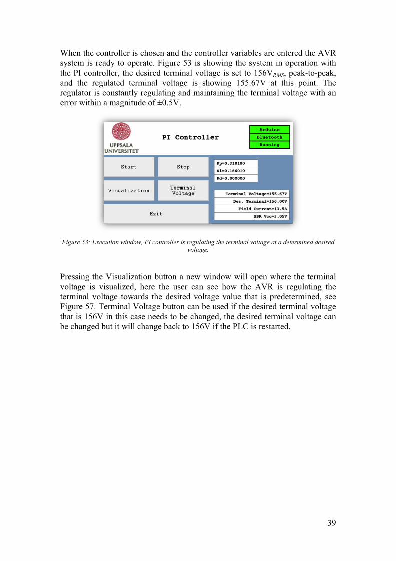
When the controller is chosen and the controller variables are entered the AVR system is ready to operate. Figure 53 is showing the system in operation with the PI controller, the desired terminal voltage is set to 156VRMS, peak-to-peak, and the regulated terminal voltage is showing 155.67V at this point. The regulator is constantly regulating and maintaining the terminal voltage with an error within a magnitude of ±0.5V.

Figure 53: Execution window, PI controller is regulating the terminal voltage at a determined desired

voltage.

Pressing the Visualization button a new window will open where the terminal voltage is visualized, here the user can see how the AVR is regulating the terminal voltage towards the desired voltage value that is predetermined, see Figure 57. Terminal Voltage button can be used if the desired terminal voltage that is 156V in this case needs to be changed, the desired terminal voltage can be changed but it will change back to 156V if the PLC is restarted.

40

5 Result

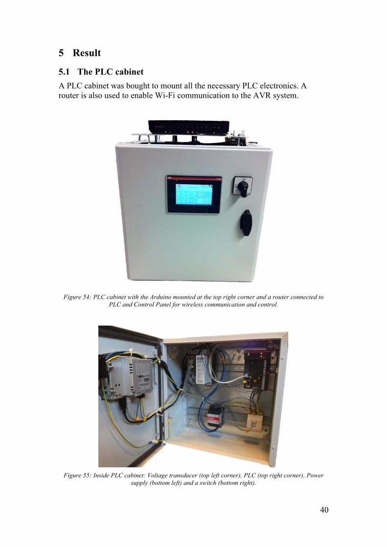
5.1 The PLC cabinet A PLC cabinet was bought to mount all the necessary PLC electronics. A router is also used to enable Wi-Fi communication to the AVR system.

Figure 54: PLC cabinet with the Arduino mounted at the top right corner and a router connected to

PLC and Control Panel for wireless communication and control.

Figure 55: Inside PLC cabinet: Voltage transducer (top left corner), PLC (top right corner), Power

supply (bottom left) and a switch (bottom right).

41

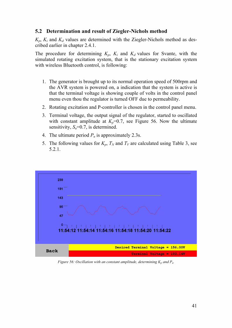
5.2 Determination and result of Ziegler-Nichols method Kp, Ki and Kd values are determined with the Ziegler-Nichols method as des-cribed earlier in chapter 2.4.1. The procedure for determining Kp, Ki and Kd values for Svante, with the simulated rotating excitation system, that is the stationary excitation system with wireless Bluetooth control, is following:

1. The generator is brought up to its normal operation speed of 500rpm and the AVR system is powered on, a indication that the system is active is that the terminal voltage is showing couple of volts in the control panel menu even thou the regulator is turned OFF due to permeability.

2. Rotating excitation and P-controller is chosen in the control panel menu. 3. Terminal voltage, the output signal of the regulator, started to oscillated

with constant amplitude at Kp=0.7, see Figure 56. Now the ultimate sensitivity, Su=0.7, is determined.

4. The ultimate period Pu is approximately 2.3s. 5. The following values for Kp, TN and TV are calculated using Table 3, see

5.2.1.

Figure 56: Oscillation with an constant amplitude, determining Kp and Pu.

42

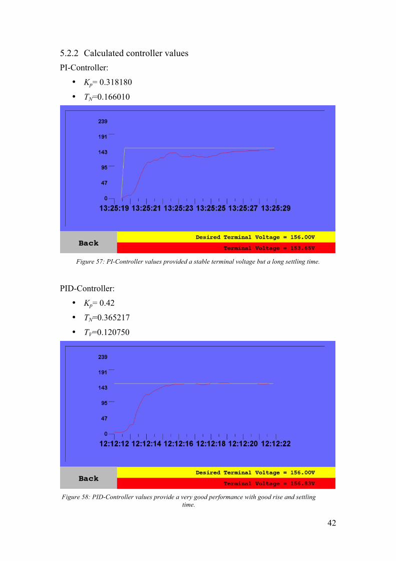
5.2.2 Calculated controller values PI-Controller:

• Kp= 0.318180

• TN=0.166010

Figure 57: PI-Controller values provided a stable terminal voltage but a long settling time.

PID-Controller:

• Kp= 0.42

• TN=0.365217

• TV=0.120750

Figure 58: PID-Controller values provide a very good performance with good rise and settling

time.

43

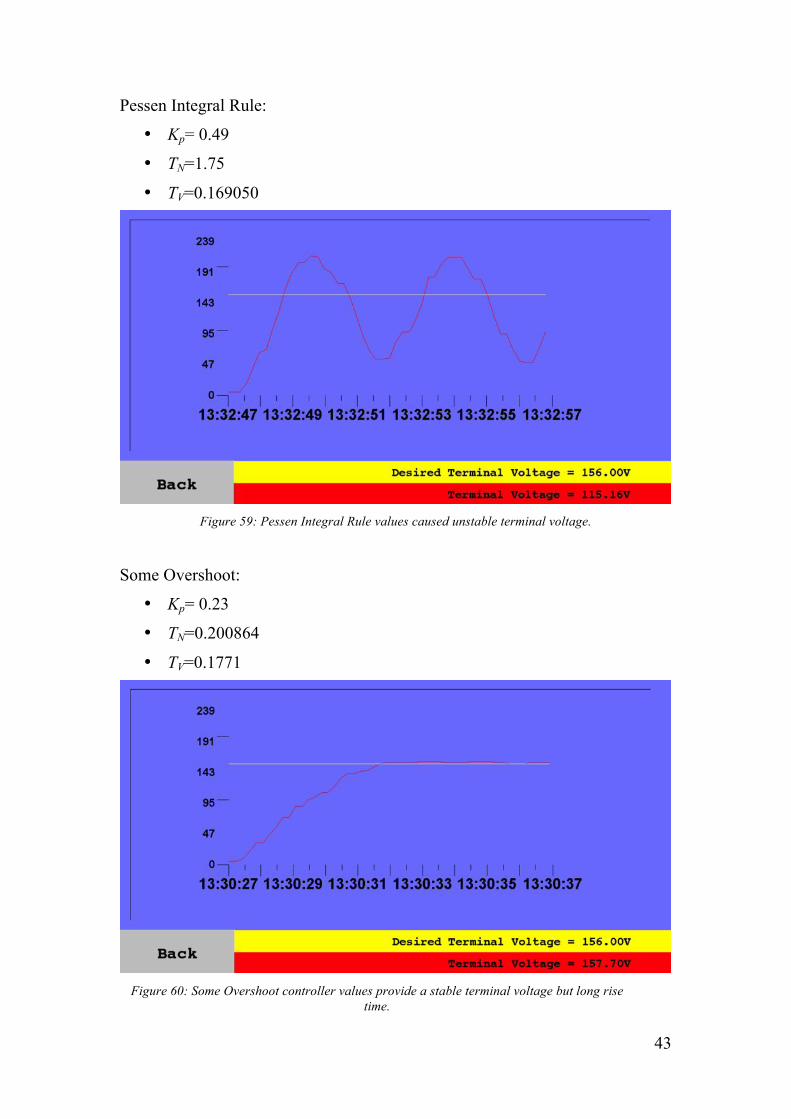
Pessen Integral Rule:

• Kp= 0.49

• TN=1.75

• TV=0.169050

Figure 59: Pessen Integral Rule values caused unstable terminal voltage.

Some Overshoot:

• Kp= 0.23

• TN=0.200864

• TV=0.1771

Figure 60: Some Overshoot controller values provide a stable terminal voltage but long rise

time.

44

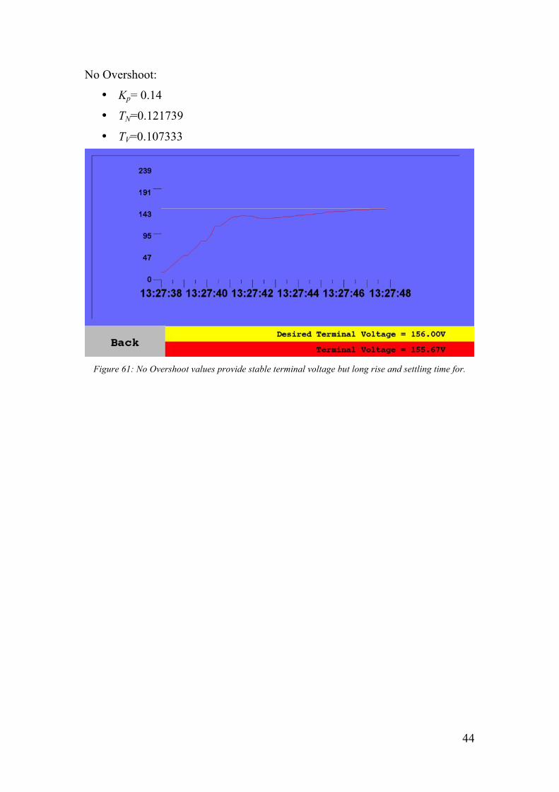
No Overshoot:

• Kp= 0.14

• TN=0.121739

• TV=0.107333

Figure 61: No Overshoot values provide stable terminal voltage but long rise and settling time for.

45

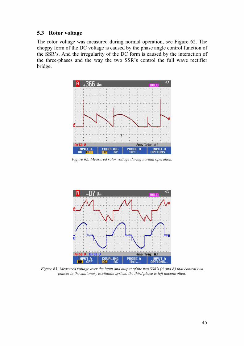
5.3 Rotor voltage The rotor voltage was measured during normal operation, see Figure 62. The choppy form of the DC voltage is caused by the phase angle control function of the SSR’s. And the irregularity of the DC form is caused by the interaction of the three-phases and the way the two SSR’s control the full wave rectifier bridge.

Figure 62: Measured rotor voltage during normal operation.

Figure 63: Measured voltage over the input and output of the two SSR's (A and B) that control two

phases in the stationary excitation system, the third phase is left uncontrolled.

46

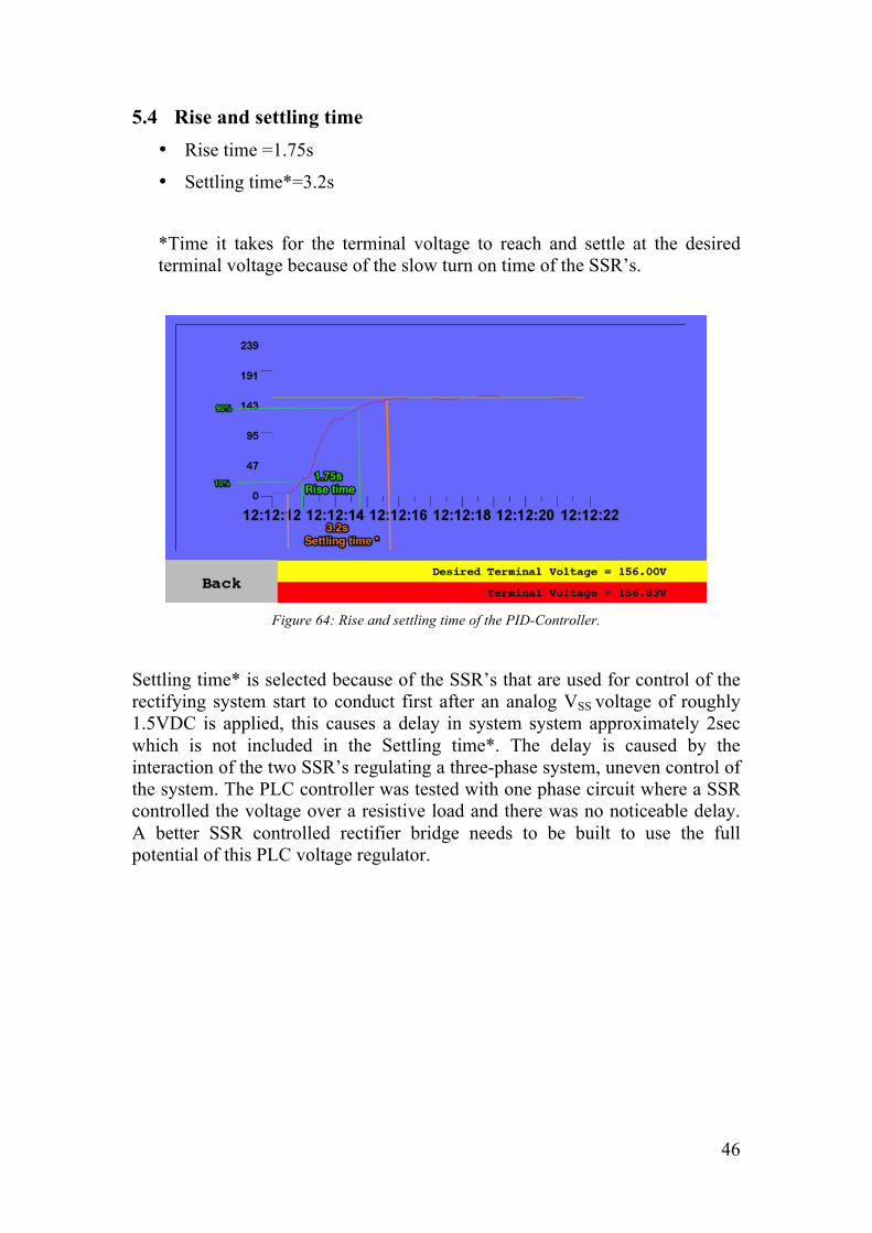
5.4 Rise and settling time • Rise time =1.75s

• Settling time*=3.2s

*Time it takes for the terminal voltage to reach and settle at the desired terminal voltage because of the slow turn on time of the SSR’s.

Figure 64: Rise and settling time of the PID-Controller.

Settling time* is selected because of the SSR’s that are used for control of the rectifying system start to conduct first after an analog VSS voltage of roughly 1.5VDC is applied, this causes a delay in system system approximately 2sec which is not included in the Settling time*. The delay is caused by the interaction of the two SSR’s regulating a three-phase system, uneven control of the system. The PLC controller was tested with one phase circuit where a SSR controlled the voltage over a resistive load and there was no noticeable delay. A better SSR controlled rectifier bridge needs to be built to use the full potential of this PLC voltage regulator.

47

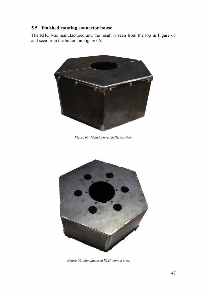
5.5 Finished rotating connector house The RHC was manufactured and the result is seen from the top in Figure 65 and seen from the bottom in Figure 66.

Figure 65: Manufactured RCH, top view.

Figure 66: Manufactured RCH, bottom view.

48

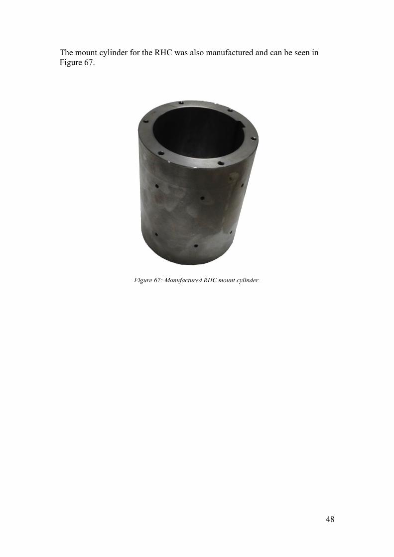
The mount cylinder for the RHC was also manufactured and can be seen in Figure 67.

Figure 67: Manufactured RHC mount cylinder.

49

6 Future work

Installation Installation of the Rotating Connector House to the generator main shaft and mounting the SSR’s, rectifier bridge, Arduino, current transducer, AC/DC- and DC/DC-converter to the RCH. Also connecting the phases from the alternator to the RCH and finally connecting the rectified power to the rotor windings. New bridge rectifier Using IGBTs or thyristors instead of diodes and making a bridge rectifier. Higher speed and resolution of the controller system Utilizing the PLC communication protocols Modbus RTU or CS31 for serial communication and changing out the Arduino Bluetooth communication to a module with RS-485 standard. This would improve the communication speed up to 187.5kBaud with a 16-bit resolution. Higher speed and resolution of the controller system with Arduino To speed up the digital to analog conversion from the rotating Arduino board to SSR’s, and to get rid of the slow PWM signal conversion to analog voltage with low-pass filter, a R-2R resistor ladder can simply be made with few resistors, R-2R resistor laddered is a very cheep and proven solution. Or a DAC, Digital to Analog Converter, can be bought and mounted instead of LP-filter, this would only improve settling time and the resolution would be the same due to Arduino’s digital output 8-bit resolution. Making a R-2R ladder network and connecting a0-a7, see Figure 68, to an Arduino’s 8 digital output pins would make a 8-bit digital to analog converter with switching speeds of 31250Hz ≈32µs, Arduino’s clock speed. If higher resolution is needed a 10-bit or 16-bit R-2R resistor ladder can be made, 5/1023=4.88mVDC for the 10-bit and 5/6553615≈15µVDC for the 16-bit R-2R. In that case the Arduino Uno would have to be replaced with the bigger Arduino Mega with 54 digital pins.

Figure 68: R-2R resistor ladder is used as a digital to analog converter [31].

50

Memory management When using the rotating excitation system or static excitation system and saving Kp, Ki and Kd values, they are all saved to same file despite the transfer function is not the same for the two systems and this may cause some confusion when switching between the two systems where one is stable and the other unstable. Or just frustrating because the Kp, Ki and Kd values have to be entered manually every time when switching between the systems. PLC code needs to be modified and a solution is to create two different files, one for the static and one for the rotating systems. These files would then be loaded from SD memory depending on which system is chosen. Re-calibrate Kp, Ki and Kd values Redo the Ziegler-Nichols method and determine new Kp, Ki and Kd values when everything is installed. The method is a good way of finding good and stabile values but it may require some further fine-tuning to get the desired controller dynamics regarding rise and setting time. Modifying current SSR’s Modifying the existing SSR’s so that they conduct only in one way and using them as 6/12 pulse thyristor rectifier, but now with the benefit where only an analog signal needs to be applied for control. Buy new SSR’s with random turn-on or DC control feature The random turn-on SSR’s seems to be a better choice than the phase angle controlled ones regarding inductive loads. It would be interesting to see the behavior of the rectifier system with random turn-on SSR’s, if it is the inductive load of the rotor windings that is causing the SSR delays and irregular shape of the DC. The DC controlled SSR would be mounted after a full wave rectifier bridge and directly control the DC voltage over the rotor winding. Further Automatization Evolve the system to be able to run some automated scenarios. For example making an Open Circuit Saturation Curve that can be time-consuming espe-cially for one person doing it manually, the PLC could be programed to do it automatically. It would be much faster process and with any desired resolution. User would just enter what maximum current level is desired and what current resolution is desired. PLC would make a file with all data needed, terminal voltage and rotor current.

51

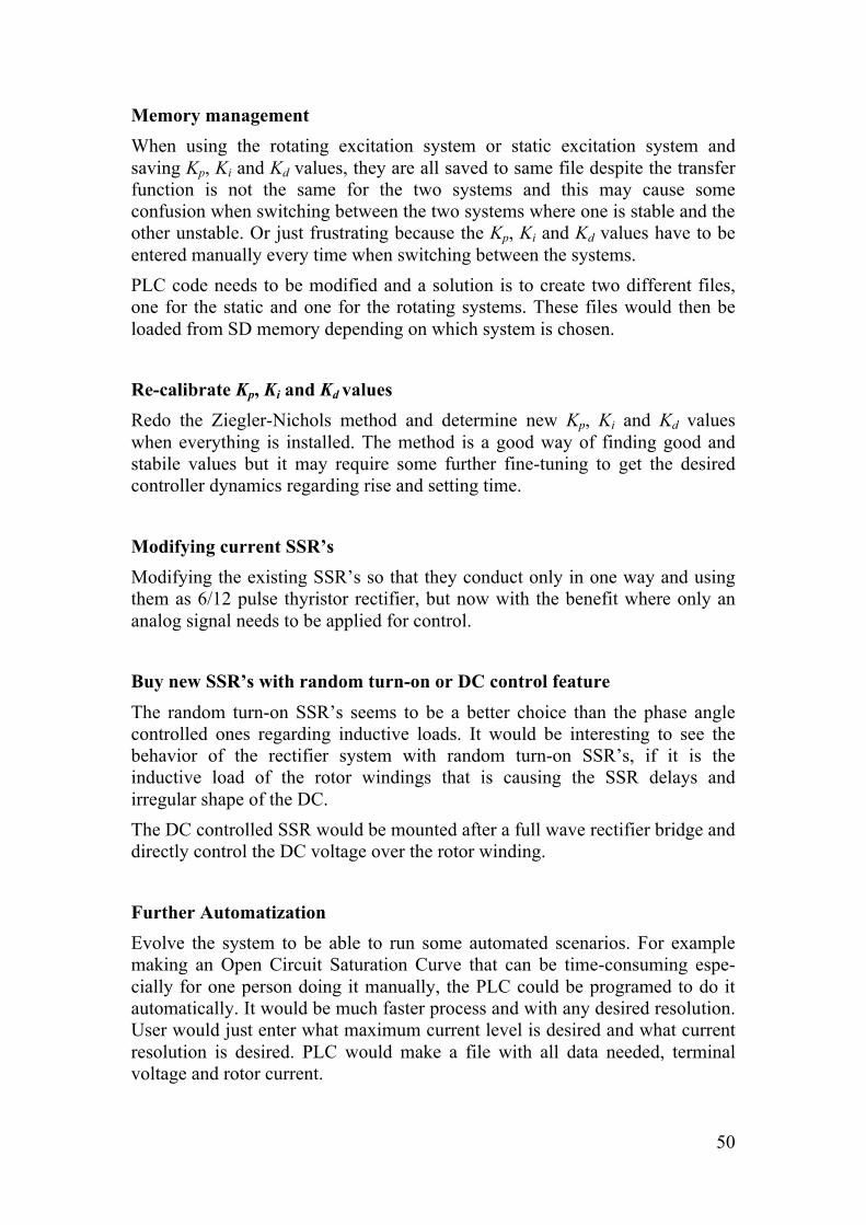
Freewheeling diode A freewheeling diode should be mounted on the rotating and stationary rectify-ing system so that the magnetic energy that is build up in the rotor windings can be safely conducted back around thru the windings and discharge instead of risking to destroying the SSR’s with a high voltage spike that can be induced by the magnetic discharge.

Figure 69: Example of a circuit with the freewheeling diode.

52

7 Evaluation and conclusion

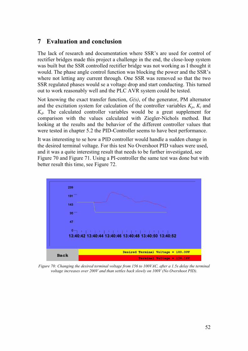
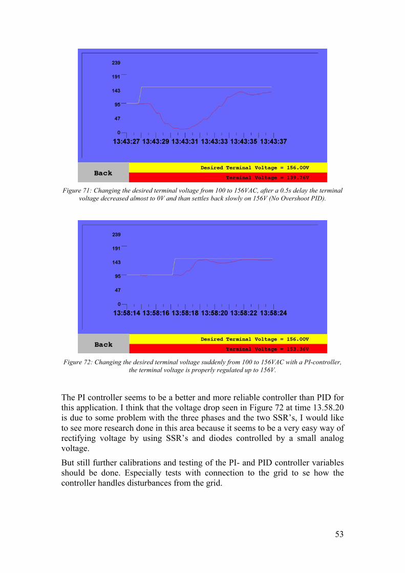
The lack of research and documentation where SSR’s are used for control of rectifier bridges made this project a challenge in the end, the close-loop system was built but the SSR controlled rectifier bridge was not working as I thought it would. The phase angle control function was blocking the power and the SSR’s where not letting any current through. One SSR was removed so that the two SSR regulated phases would se a voltage drop and start conducting. This turned out to work reasonably well and the PLC AVR system could be tested. Not knowing the exact transfer function, G(s), of the generator, PM alternator and the excitation system for calculation of the controller variables Kp, Ki and Kd. The calculated controller variables would be a great supplement for comparison with the values calculated with Ziegler-Nichols method. But looking at the results and the behavior of the different controller values that were tested in chapter 5.2 the PID-Controller seems to have best performance. It was interesting to se how a PID controller would handle a sudden change in the desired terminal voltage. For this test No Overshoot PID values were used, and it was a quite interesting result that needs to be further investigated, see Figure 70 and Figure 71. Using a PI-controller the same test was done but with better result this time, see Figure 72.

Figure 70: Changing the desired terminal voltage from 156 to 100VAC, after a 1.5s delay the terminal

voltage increases over 200V and than settles back slowly on 100V (No Overshoot PID).

53

Figure 71: Changing the desired terminal voltage from 100 to 156VAC, after a 0.5s delay the terminal

voltage decreased almost to 0V and than settles back slowly on 156V (No Overshoot PID).

Figure 72: Changing the desired terminal voltage suddenly from 100 to 156VAC with a PI-controller,

the terminal voltage is properly regulated up to 156V.

The PI controller seems to be a better and more reliable controller than PID for this application. I think that the voltage drop seen in Figure 72 at time 13.58.20 is due to some problem with the three phases and the two SSR’s, I would like to see more research done in this area because it seems to be a very easy way of rectifying voltage by using SSR’s and diodes controlled by a small analog voltage. But still further calibrations and testing of the PI- and PID controller variables should be done. Especially tests with connection to the grid to se how the controller handles disturbances from the grid.

54

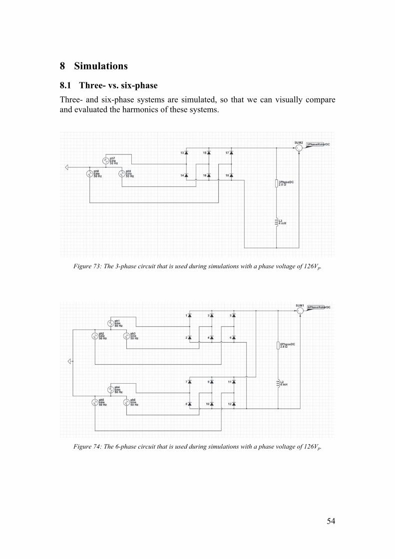
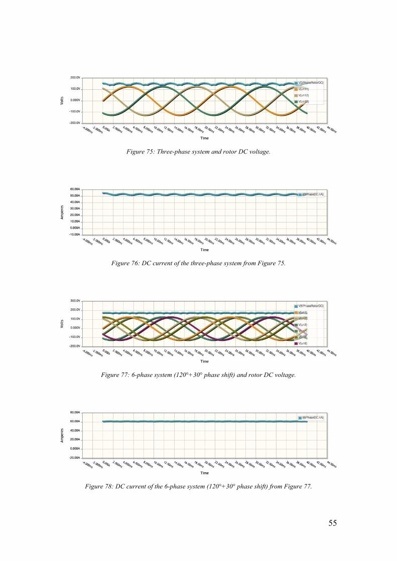
8 Simulations

8.1 Three- vs. six-phase Three- and six-phase systems are simulated, so that we can visually compare and evaluated the harmonics of these systems.

Figure 73: The 3-phase circuit that is used during simulations with a phase voltage of 126Vp.

Figure 74: The 6-phase circuit that is used during simulations with a phase voltage of 126Vp.

55

Figure 75: Three-phase system and rotor DC voltage.

Figure 76: DC current of the three-phase system from Figure 75.

Figure 77: 6-phase system (120°+30° phase shift) and rotor DC voltage.

Figure 78: DC current of the 6-phase system (120°+30° phase shift) from Figure 77.

56

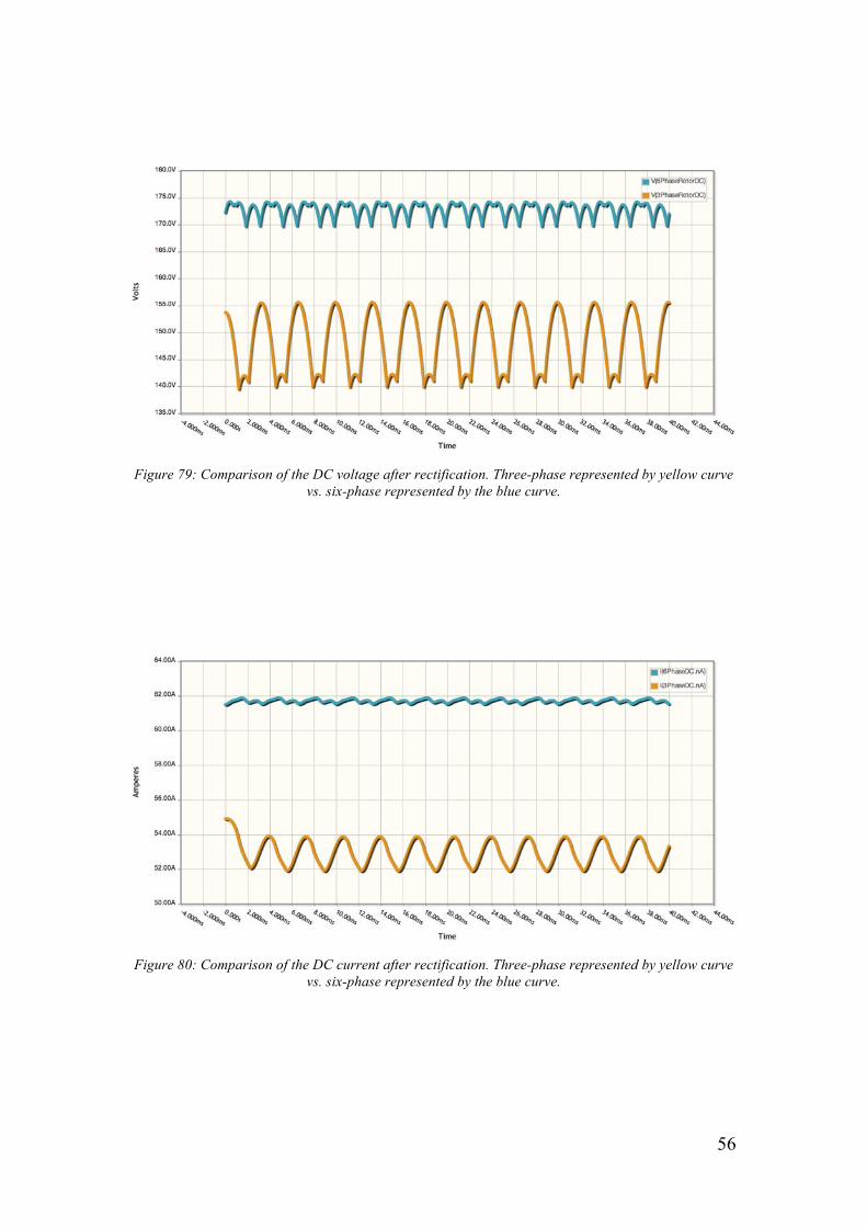
Figure 79: Comparison of the DC voltage after rectification. Three-phase represented by yellow curve

vs. six-phase represented by the blue curve.

Figure 80: Comparison of the DC current after rectification. Three-phase represented by yellow curve

vs. six-phase represented by the blue curve.

57

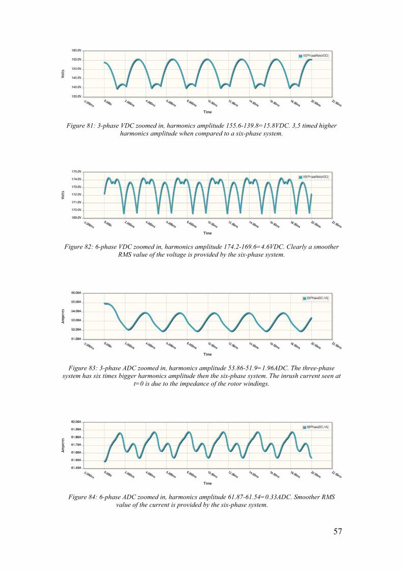
Figure 81: 3-phase VDC zoomed in, harmonics amplitude 155.6-139.8=15.8VDC. 3,5 timed higher

harmonics amplitude when compared to a six-phase system.

Figure 82: 6-phase VDC zoomed in, harmonics amplitude 174.2-169.6=4.6VDC. Clearly a smoother

RMS value of the voltage is provided by the six-phase system.

Figure 83: 3-phase ADC zoomed in, harmonics amplitude 53.86-51.9=1.96ADC. The three-phase

system has six times bigger harmonics amplitude then the six-phase system. The inrush current seen at t=0 is due to the impedance of the rotor windings.

Figure 84: 6-phase ADC zoomed in, harmonics amplitude 61.87-61.54=0.33ADC. Smoother RMS

value of the current is provided by the six-phase system.

58

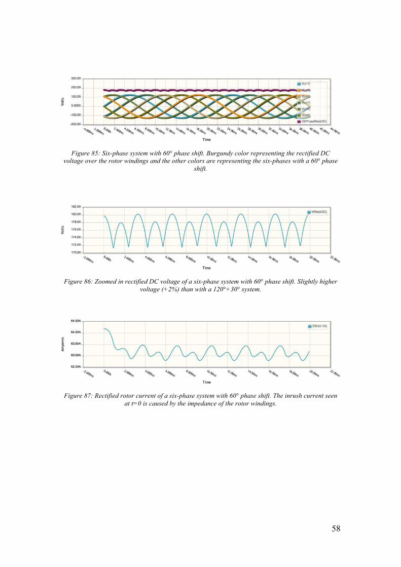
Figure 85: Six-phase system with 60° phase shift. Burgundy color representing the rectified DC

voltage over the rotor windings and the other colors are representing the six-phases with a 60° phase shift.

Figure 86: Zoomed in rectified DC voltage of a six-phase system with 60° phase shift. Slightly higher

voltage (+2%) than with a 120°+30° system.

Figure 87: Rectified rotor current of a six-phase system with 60° phase shift. The inrush current seen

at t=0 is caused by the impedance of the rotor windings.

59

8.2 Differential amplifier

Figure 88: Differential Amplifier plotted with the two input signals and the output voltage. At the left

hand side the difference is 2,5VDC between the input signals and the differential amplifier is amplifying the difference with a gain of two so the output voltage is 5VDC and at the right hand side

the difference is 0VDC so the output is 0VDC.

8.3 Conclusion By studying the simulations of six- and the three-phase systems it is clear that the six-phase system has much lower harmonics than the three-phase system and it is a more preferable choice for this application, see Figure 79 and Figure 80. The theory of a differential amplifier is explained in chapter 3.5 and the goal was to double the resolution of the current transducer with a differential amplifier circuit. The result of such circuit can be seen in Figure 88 where the difference of the two input signals is doubled.

60

References

[1] Prabha Kundur, Power Systems Stability and Control, Electric Power Research Institute, January 1994.

[2] Gene F. Franklin, J. David Powell, Abbas Emami-Naeini, Feedback Control of Dynamic Systems, Fifth Edition, 2005.

[3] David Benyon, Phil Turner, Susan Turner, Designing Interactive Systems, Addison-Wesley 2005.

[4] Lars-Hugo Hemert, Digitala kretsar, Division of Electricity, Studentliteratur, 1996.

[5] Bengt Molin, Analog elektronik, Studentliteratur, 2001.

[6] Mattias Wallin, An experimental generator test setup for hydropower research and model verification, Division of Electricity, Uppsala University, January 2011.

[7] Mattias Wallin, Measurement and modeling of unbalanced magnetic pull in hydropower generators, Division of Electricity, Uppsala University, April 2013.

[8] Erica Lindström, Rotor resistans mätning, Division of Electricity, Uppsala University, 2012.

[9] http://web.ing.puc.cl/~power/paperspdf/dixon/21.pdf, June 2013.

[10] http://www05.abb.com/global/scot/scot209.nsf/veritydisplay/4983602c6751527bc125739f002abf0b/$file/2cdc125021m0202.pdf, June 2013.

[11] http://www.parkermotion.com/manuals/Hauser/Compax3/CoDeSys_Manual_V2p3.pdf, June 2013.

[12] http://www.fameview.com/download/src/AC500-eCo-Hardware.pdf, June 2013.

[13] J.G Ziegler and N.B Nicholds, Optimum Setting for Automatic Controllers, Rochester, N.Y.

[14] Finn Haugen, Ziegler-Nichols’ Closed-Loop Method, TechTeach 17. July 2010.

[15] http://www.omron-ap.com/FAQ/FAQ02153/index.asp, June 2013.

[16] http://www.crydom.com/en/Tech/Newsletters/Solid%20Statements%20-%20SSRs%20switching%20types.pdf, June 2013.

[17] http://www.ampbooks.com/home/amplifier-calculators/RC-ripple-filter/, June 2013.

[18] http://commons.wikimedia.org/wiki/File:Butterworth_response.svg, June 2013.

[19] Juan de Santiago, Excitation Systems for Synchronous Generators, Uppsala University.

61

[20] http://upload.wikimedia.org/wikipedia/commons/2/24/Feedback_loop_with_descriptions.svg, June 2013.

[21] http://octopart.com/csla1ce-honeywell-1803194, June 2013.

[22] http://www.ti.com/lit/ds/sbos077b/sbos077b.pdf, June 2013.

[23] http://www.crydom.com/en/products/catalog/m_cpc.pdf, June 2013.

[24] http://sim.okawa-denshi.jp/en/PWMtool.php, June 2013.

[25] http://www.tillquist.com/kraftautomation/kategorier/matvardesomvandlare/spanning-ac/u420?highlight=YToxOntpOjA7czo0OiJ1NDIwIjt9, June 2013.

[26] https://www.elfa.se/elfa3~tr_en/elfa/init.do?item=70-003-15&toc=19084, June 2013.

[27] http://www.tracopower.com/products/ten40wir.pdf, June 2013.

[28] http://www.abb.com/product/seitp329/6b9c7e5f00fb4961c125790600299bbc.aspx?country=00&tabKey=2&cid=9AAC124505&gid=ABB1SAP520100R0001, June 2013.

[29] http://www.abb.com/product/seitp329/be2c616b9f2fc3e2c1256ff00047a8f2.aspx?tabKey=2&gid=ABB1TNE968900R1110&cid=9AAC100147, June 2013.

[30] http://www.codesys.com, June 2013.

[31] http://upload.wikimedia.org/wikipedia/commons/thumb/4/41/R2r-ladder.png/420px-R2r-ladder.png, June 2013.

62

9 Appendix

PLC code PLC_PRG

0001 (*Main program*)00020003 PROGRAM PLC_PRG0004 VAR0005 Conv: Converter;0006 Regulator_p_i_d: Regulator;0007 Mode_box: Mode;00080009 Terminal_Voltage: REAL;00100011 Regulator_Output_Voltage: REAL;0012 Var_desired_value: REAL;00130014 Run: BOOL;00150016 Meassured_Field_Current: REAL;0017 Read_save1: SD_Save_Read;00180019 Numpad_BoYo: Numpad_B;0020 NumP_1: BOOL;0021 NumP_2: BOOL;0022 NumP_3: BOOL;0023 NumP_4: BOOL;0024 NumP_5: BOOL;0025 NumP_6: BOOL;0026 NumP_7: BOOL;0027 NumP_8: BOOL;0028 NumP_9: BOOL;0029 NumP_0: BOOL;0030 NumP_Dot: BOOL;0031 NumP_Clear: BOOL;0032 NumP_OK: BOOL;00330034 Load_Configuration: BOOL;0035 Load_Last_Configuration: BOOL;0036 Save_button: BOOL;00370038 Load_Last_timer: TP;0039 Load_Last_time: TIME:=T#500ms;0040 Conversion: KiKd_to_TnTv;0041 StaticOrRotating: Static_or_Rotating;0042 Static: BOOL;0043 Rotating: BOOL;0044 END_VAR00450046 VAR_INPUT00470048 END_VAR0049

63

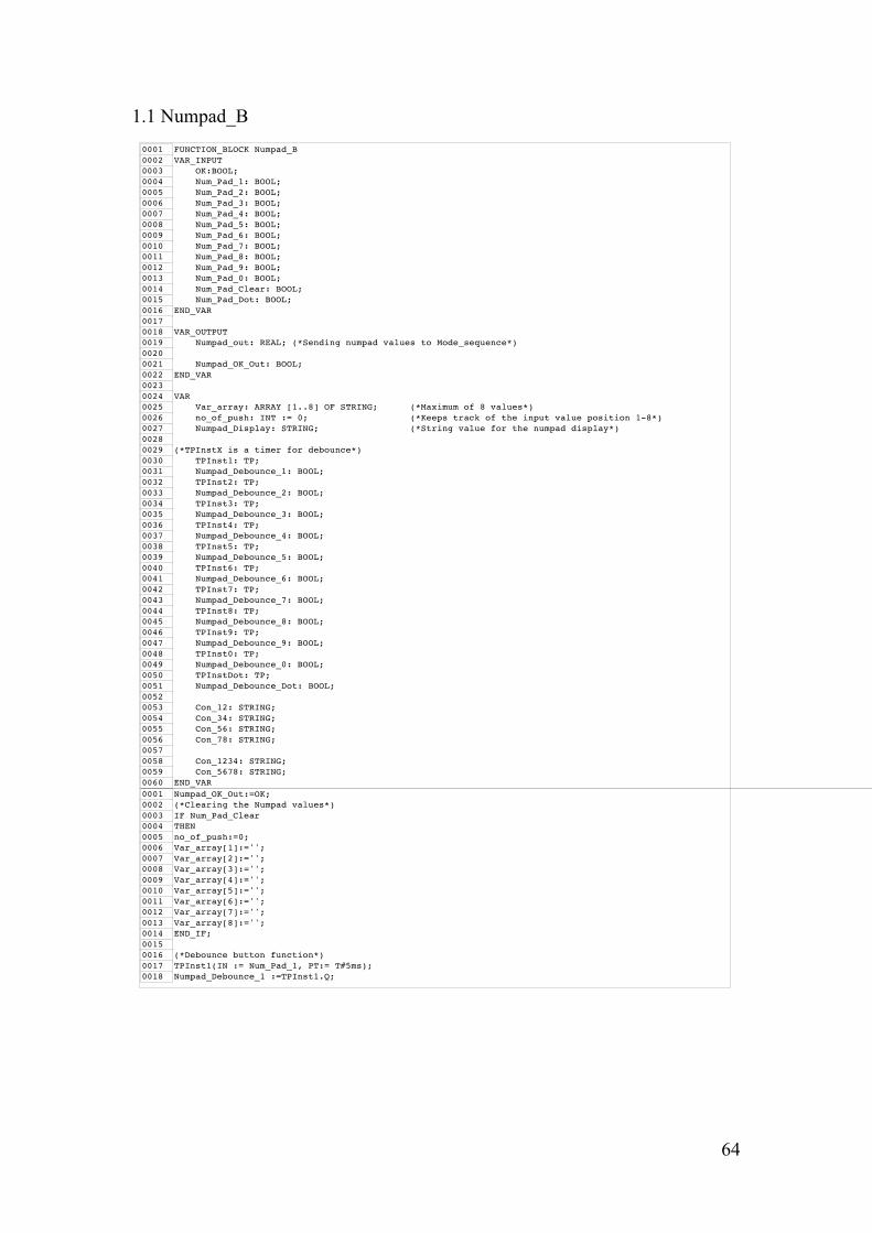
64

1.1 Numpad_B

0001 FUNCTION_BLOCK Numpad_B0002 VAR_INPUT0003 OK:BOOL;0004 Num_Pad_1: BOOL;0005 Num_Pad_2: BOOL;0006 Num_Pad_3: BOOL;0007 Num_Pad_4: BOOL;0008 Num_Pad_5: BOOL;0009 Num_Pad_6: BOOL;0010 Num_Pad_7: BOOL;0011 Num_Pad_8: BOOL;0012 Num_Pad_9: BOOL;0013 Num_Pad_0: BOOL;0014 Num_Pad_Clear: BOOL;0015 Num_Pad_Dot: BOOL;0016 END_VAR00170018 VAR_OUTPUT0019 Numpad_out: REAL; (*Sending numpad values to Mode_sequence*)00200021 Numpad_OK_Out: BOOL;0022 END_VAR00230024 VAR0025 Var_array: ARRAY [1..8] OF STRING; (*Maximum of 8 values*)0026 no_of_push: INT := 0; (*Keeps track of the input value position 1-8*)0027 Numpad_Display: STRING; (*String value for the numpad display*)00280029 (*TPInstX is a timer for debounce*)0030 TPInst1: TP;0031 Numpad_Debounce_1: BOOL;0032 TPInst2: TP;0033 Numpad_Debounce_2: BOOL;0034 TPInst3: TP;0035 Numpad_Debounce_3: BOOL;0036 TPInst4: TP;0037 Numpad_Debounce_4: BOOL;0038 TPInst5: TP;0039 Numpad_Debounce_5: BOOL;0040 TPInst6: TP;0041 Numpad_Debounce_6: BOOL;0042 TPInst7: TP;0043 Numpad_Debounce_7: BOOL;0044 TPInst8: TP;0045 Numpad_Debounce_8: BOOL;0046 TPInst9: TP;0047 Numpad_Debounce_9: BOOL;0048 TPInst0: TP;0049 Numpad_Debounce_0: BOOL;0050 TPInstDot: TP;0051 Numpad_Debounce_Dot: BOOL;00520053 Con_12: STRING;0054 Con_34: STRING;0055 Con_56: STRING;0056 Con_78: STRING;00570058 Con_1234: STRING;0059 Con_5678: STRING;0060 END_VAR0001 Numpad_OK_Out:=OK;0002 (*Clearing the Numpad values*)0003 IF Num_Pad_Clear0004 THEN0005 no_of_push:=0;0006 Var_array[1]:='';0007 Var_array[2]:='';0008 Var_array[3]:='';0009 Var_array[4]:='';0010 Var_array[5]:='';0011 Var_array[6]:='';0012 Var_array[7]:='';0013 Var_array[8]:='';0014 END_IF;00150016 (*Debounce button function*)0017 TPInst1(IN := Num_Pad_1, PT:= T#5ms);0018 Numpad_Debounce_1 :=TPInst1.Q;

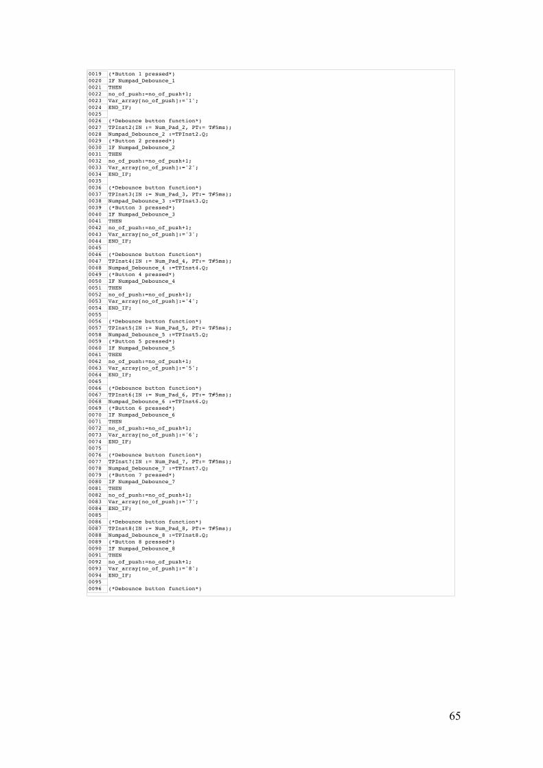
65

0019 (*Button 1 pressed*)0020 IF Numpad_Debounce_10021 THEN0022 no_of_push:=no_of_push+1;0023 Var_array[no_of_push]:='1';0024 END_IF;00250026 (*Debounce button function*)0027 TPInst2(IN := Num_Pad_2, PT:= T#5ms);0028 Numpad_Debounce_2 :=TPInst2.Q;0029 (*Button 2 pressed*)0030 IF Numpad_Debounce_20031 THEN0032 no_of_push:=no_of_push+1;0033 Var_array[no_of_push]:='2';0034 END_IF;00350036 (*Debounce button function*)0037 TPInst3(IN := Num_Pad_3, PT:= T#5ms);0038 Numpad_Debounce_3 :=TPInst3.Q;0039 (*Button 3 pressed*)0040 IF Numpad_Debounce_30041 THEN0042 no_of_push:=no_of_push+1;0043 Var_array[no_of_push]:='3';0044 END_IF;00450046 (*Debounce button function*)0047 TPInst4(IN := Num_Pad_4, PT:= T#5ms);0048 Numpad_Debounce_4 :=TPInst4.Q;0049 (*Button 4 pressed*)0050 IF Numpad_Debounce_40051 THEN0052 no_of_push:=no_of_push+1;0053 Var_array[no_of_push]:='4';0054 END_IF;00550056 (*Debounce button function*)0057 TPInst5(IN := Num_Pad_5, PT:= T#5ms);0058 Numpad_Debounce_5 :=TPInst5.Q;0059 (*Button 5 pressed*)0060 IF Numpad_Debounce_50061 THEN0062 no_of_push:=no_of_push+1;0063 Var_array[no_of_push]:='5';0064 END_IF;00650066 (*Debounce button function*)0067 TPInst6(IN := Num_Pad_6, PT:= T#5ms);0068 Numpad_Debounce_6 :=TPInst6.Q;0069 (*Button 6 pressed*)0070 IF Numpad_Debounce_60071 THEN0072 no_of_push:=no_of_push+1;0073 Var_array[no_of_push]:='6';0074 END_IF;00750076 (*Debounce button function*)0077 TPInst7(IN := Num_Pad_7, PT:= T#5ms);0078 Numpad_Debounce_7 :=TPInst7.Q;0079 (*Button 7 pressed*)0080 IF Numpad_Debounce_70081 THEN0082 no_of_push:=no_of_push+1;0083 Var_array[no_of_push]:='7';0084 END_IF;00850086 (*Debounce button function*)0087 TPInst8(IN := Num_Pad_8, PT:= T#5ms);0088 Numpad_Debounce_8 :=TPInst8.Q;0089 (*Button 8 pressed*)0090 IF Numpad_Debounce_80091 THEN0092 no_of_push:=no_of_push+1;0093 Var_array[no_of_push]:='8';0094 END_IF;00950096 (*Debounce button function*)

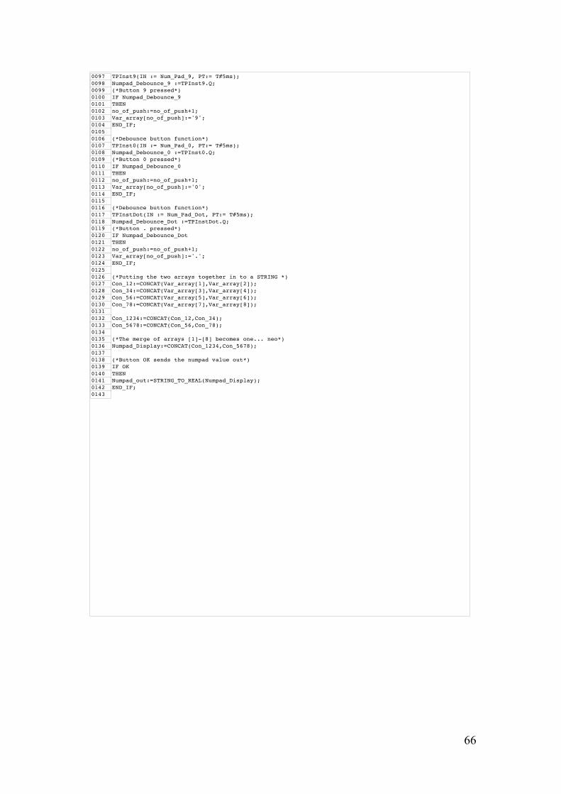
66

0097 TPInst9(IN := Num_Pad_9, PT:= T#5ms);0098 Numpad_Debounce_9 :=TPInst9.Q;0099 (*Button 9 pressed*)0100 IF Numpad_Debounce_90101 THEN0102 no_of_push:=no_of_push+1;0103 Var_array[no_of_push]:='9';0104 END_IF;01050106 (*Debounce button function*)0107 TPInst0(IN := Num_Pad_0, PT:= T#5ms);0108 Numpad_Debounce_0 :=TPInst0.Q;0109 (*Button 0 pressed*)0110 IF Numpad_Debounce_00111 THEN0112 no_of_push:=no_of_push+1;0113 Var_array[no_of_push]:='0';0114 END_IF;01150116 (*Debounce button function*)0117 TPInstDot(IN := Num_Pad_Dot, PT:= T#5ms);0118 Numpad_Debounce_Dot :=TPInstDot.Q;0119 (*Button . pressed*)0120 IF Numpad_Debounce_Dot0121 THEN0122 no_of_push:=no_of_push+1;0123 Var_array[no_of_push]:='.';0124 END_IF;01250126 (*Putting the two arrays together in to a STRING *)0127 Con_12:=CONCAT(Var_array[1],Var_array[2]);0128 Con_34:=CONCAT(Var_array[3],Var_array[4]);0129 Con_56:=CONCAT(Var_array[5],Var_array[6]);0130 Con_78:=CONCAT(Var_array[7],Var_array[8]);01310132 Con_1234:=CONCAT(Con_12,Con_34);0133 Con_5678:=CONCAT(Con_56,Con_78);01340135 (*The merge of arrays [1]-[8] becomes one... neo*)0136 Numpad_Display:=CONCAT(Con_1234,Con_5678);01370138 (*Button OK sends the numpad value out*)0139 IF OK0140 THEN0141 Numpad_out:=STRING_TO_REAL(Numpad_Display);0142 END_IF;0143

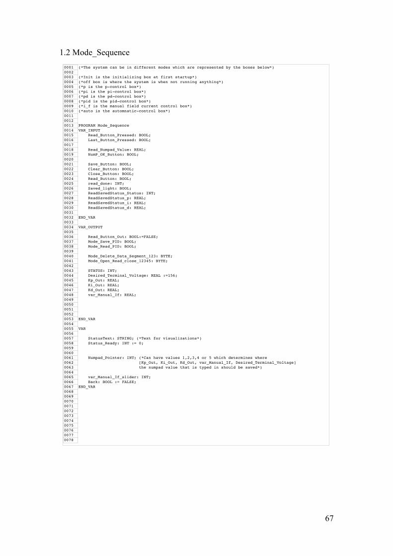
67

1.2 Mode_Sequence

0001 (*The system can be in different modes which are represented by the boxes below*)00020003 (*Init is the initializing box at first startup*)0004 (*off box is where the system is when not running anything*)0005 (*p is the p-control box*)0006 (*pi is the pi-control box*)0007 (*pd is the pd-control box*)0008 (*pid is the pid-control box*)0009 (*i_f is the manual field current control box*)0010 (*auto is the automnatic-control box*)001100120013 PROGRAM Mode_Sequence0014 VAR_INPUT0015 Read_Button_Pressed: BOOL;0016 Last_Button_Pressed: BOOL;00170018 Read_Numpad_Value: REAL;0019 NumP_OK_Button: BOOL;00200021 Save_Button: BOOL;0022 Clear_Button: BOOL;0023 Close_Button: BOOL;0024 Read_Button: BOOL;0025 read_done: INT;0026 Saved_light: BOOL;0027 ReadSavedStatus_Status: INT;0028 ReadSavedStatus_p: REAL;0029 ReadSavedStatus_i: REAL;0030 ReadSavedStatus_d: REAL;00310032 END_VAR00330034 VAR_OUTPUT00350036 Read_Button_Out: BOOL:=FALSE;0037 Mode_Save_PID: BOOL;0038 Mode_Read_PID: BOOL;00390040 Mode_Delete_Data_Segment_123: BYTE;0041 Mode_Open_Read_close_12345: BYTE;00420043 STATUS: INT;0044 Desired_Terminal_Voltage: REAL :=156;0045 Kp_Out: REAL;0046 Ki_Out: REAL;0047 Kd_Out: REAL;0048 var_Manual_If: REAL;00490050005100520053 END_VAR00540055 VAR00560057 StatusText: STRING; (*Text for visualizations*)0058 Status_Ready: INT := 0;005900600061 Numpad_Pointer: INT; (*Can have values 1,2,3,4 or 5 which determines where0062 [Kp_Out, Ki_Out, Kd_Out, var_Manual_If, Desired_Terminal_Voltage]0063 the numpad value that is typed in should be saved*)00640065 var_Manual_If_slider: INT;0066 Back: BOOL := FALSE;0067 END_VAR00680069007000710072007300740075007600770078

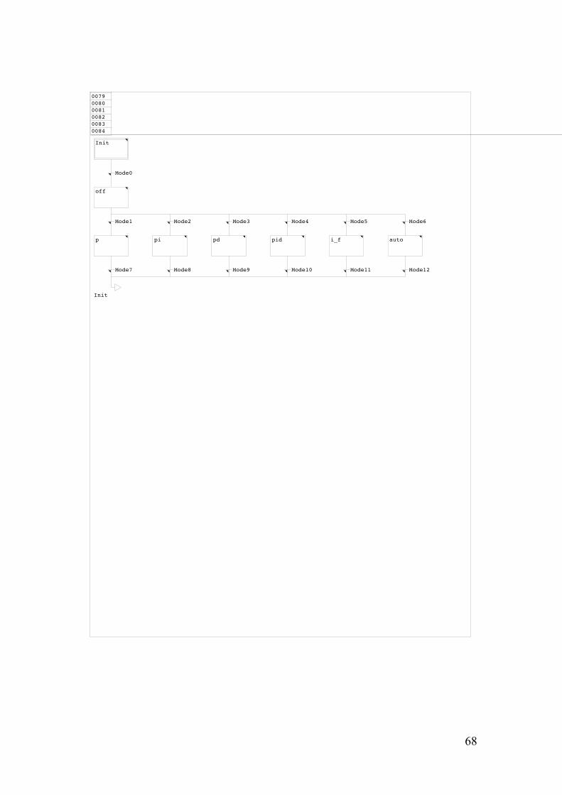
68

007900800081008200830084

Init

Mode0

off

Mode1

p

Mode7

Mode2

pi

Mode8

Mode3

pd

Mode9

Mode4

pid

Mode10

Mode5

i_f

Mode11

Mode6

auto

Mode12

Init

69

1.2.1 Init

0001 (*Determinating if back button is used or exit button, to read or not to read, that is the question *)00020003 IF Back AND NOT Saved_light0004 THEN0005 Status:=0;0006 ELSE0007 Read_Button_Out:=TRUE;0008 Status:=0;0009 digital_output_0:=FALSE; (*turn of static SSR's when "YES" button is used from AUTO_exit*)0010 END_IF;

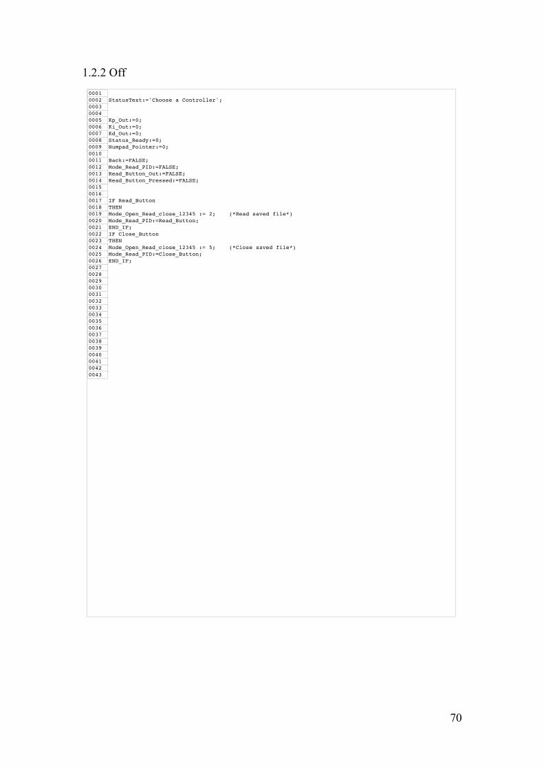
70

1.2.2 Off

00010002 StatusText:='Choose a Controller';000300040005 Kp_Out:=0;0006 Ki_Out:=0;0007 Kd_Out:=0;0008 Status_Ready:=0;0009 Numpad_Pointer:=0;00100011 Back:=FALSE;0012 Mode_Read_PID:=FALSE;0013 Read_Button_Out:=FALSE;0014 Read_Button_Pressed:=FALSE;001500160017 IF Read_Button0018 THEN0019 Mode_Open_Read_close_12345 := 2; (*Read saved file*)0020 Mode_Read_PID:=Read_Button;0021 END_IF;0022 IF Close_Button0023 THEN0024 Mode_Open_Read_close_12345 := 5; (*Close saved file*)0025 Mode_Read_PID:=Close_Button;0026 END_IF;00270028002900300031003200330034003500360037003800390040004100420043

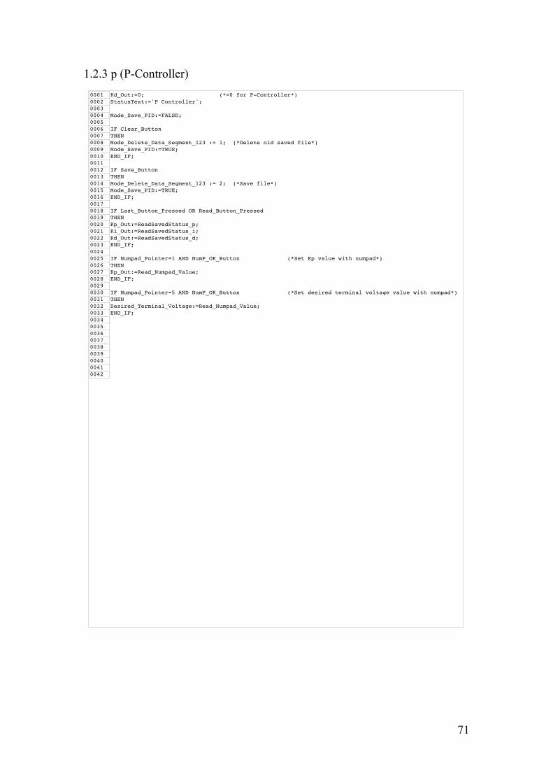
71

1.2.3 p (P-Controller)

0001 Kd_Out:=0; (*=0 for P-Controller*)0002 StatusText:='P Controller';00030004 Mode_Save_PID:=FALSE;00050006 IF Clear_Button0007 THEN0008 Mode_Delete_Data_Segment_123 := 1; (*Delete old saved file*)0009 Mode_Save_PID:=TRUE;0010 END_IF;00110012 IF Save_Button0013 THEN0014 Mode_Delete_Data_Segment_123 := 2; (*Save file*)0015 Mode_Save_PID:=TRUE;0016 END_IF;00170018 IF Last_Button_Pressed OR Read_Button_Pressed0019 THEN0020 Kp_Out:=ReadSavedStatus_p;0021 Ki_Out:=ReadSavedStatus_i;0022 Kd_Out:=ReadSavedStatus_d;0023 END_IF;00240025 IF Numpad_Pointer=1 AND NumP_OK_Button (*Set Kp value with numpad*)0026 THEN0027 Kp_Out:=Read_Numpad_Value;0028 END_IF;00290030 IF Numpad_Pointer=5 AND NumP_OK_Button (*Set desired terminal voltage value with numpad*)0031 THEN0032 Desired_Terminal_Voltage:=Read_Numpad_Value;0033 END_IF;003400350036003700380039004000410042

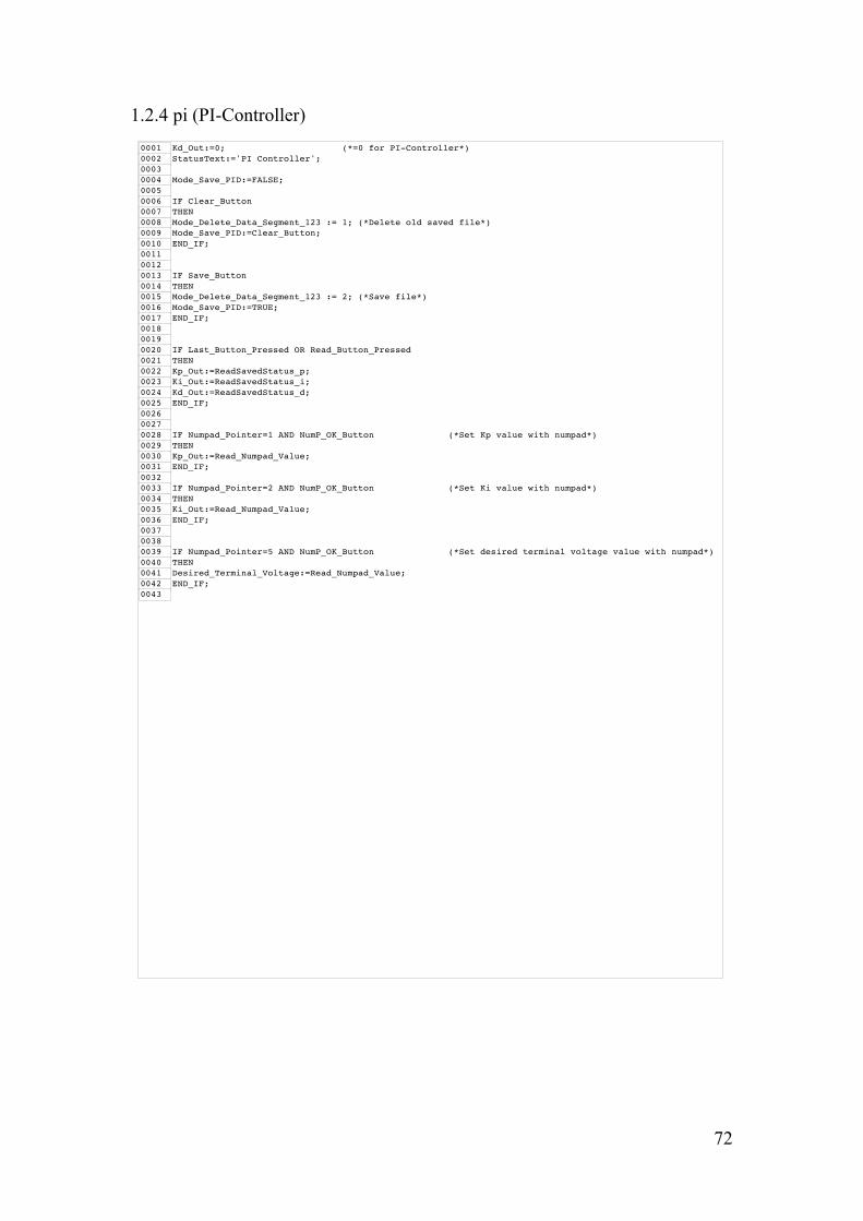
72

1.2.4 pi (PI-Controller)

0001 Kd_Out:=0; (*=0 for PI-Controller*)0002 StatusText:='PI Controller';00030004 Mode_Save_PID:=FALSE;00050006 IF Clear_Button0007 THEN0008 Mode_Delete_Data_Segment_123 := 1; (*Delete old saved file*)0009 Mode_Save_PID:=Clear_Button;0010 END_IF;001100120013 IF Save_Button0014 THEN0015 Mode_Delete_Data_Segment_123 := 2; (*Save file*)0016 Mode_Save_PID:=TRUE;0017 END_IF;001800190020 IF Last_Button_Pressed OR Read_Button_Pressed0021 THEN0022 Kp_Out:=ReadSavedStatus_p;0023 Ki_Out:=ReadSavedStatus_i;0024 Kd_Out:=ReadSavedStatus_d;0025 END_IF;002600270028 IF Numpad_Pointer=1 AND NumP_OK_Button (*Set Kp value with numpad*)0029 THEN0030 Kp_Out:=Read_Numpad_Value;0031 END_IF;00320033 IF Numpad_Pointer=2 AND NumP_OK_Button (*Set Ki value with numpad*)0034 THEN0035 Ki_Out:=Read_Numpad_Value;0036 END_IF;003700380039 IF Numpad_Pointer=5 AND NumP_OK_Button (*Set desired terminal voltage value with numpad*)0040 THEN0041 Desired_Terminal_Voltage:=Read_Numpad_Value;0042 END_IF;0043

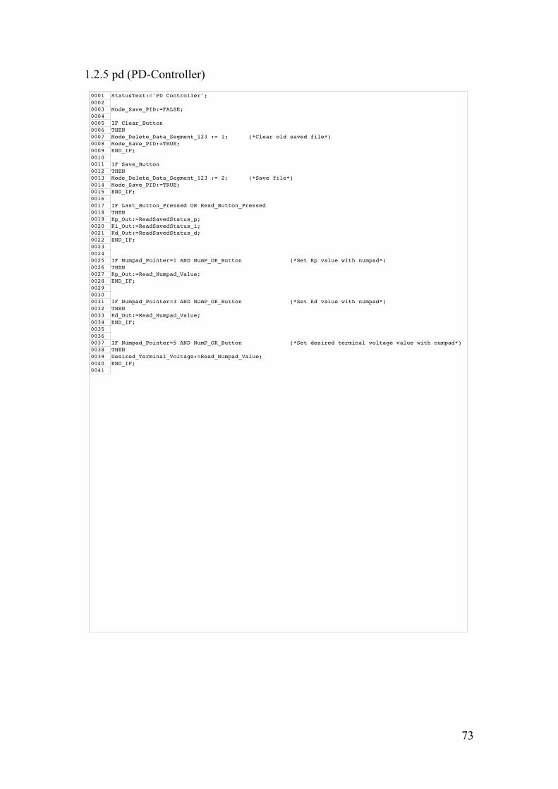
73

1.2.5 pd (PD-Controller)

0001 StatusText:='PD Controller';00020003 Mode_Save_PID:=FALSE;00040005 IF Clear_Button0006 THEN0007 Mode_Delete_Data_Segment_123 := 1; (*Clear old saved file*)0008 Mode_Save_PID:=TRUE;0009 END_IF;00100011 IF Save_Button0012 THEN0013 Mode_Delete_Data_Segment_123 := 2; (*Save file*)0014 Mode_Save_PID:=TRUE;0015 END_IF;00160017 IF Last_Button_Pressed OR Read_Button_Pressed0018 THEN0019 Kp_Out:=ReadSavedStatus_p;0020 Ki_Out:=ReadSavedStatus_i;0021 Kd_Out:=ReadSavedStatus_d;0022 END_IF;002300240025 IF Numpad_Pointer=1 AND NumP_OK_Button (*Set Kp value with numpad*)0026 THEN0027 Kp_Out:=Read_Numpad_Value;0028 END_IF;002900300031 IF Numpad_Pointer=3 AND NumP_OK_Button (*Set Kd value with numpad*)0032 THEN0033 Kd_Out:=Read_Numpad_Value;0034 END_IF;003500360037 IF Numpad_Pointer=5 AND NumP_OK_Button (*Set desired terminal voltage value with numpad*)0038 THEN0039 Desired_Terminal_Voltage:=Read_Numpad_Value;0040 END_IF;0041

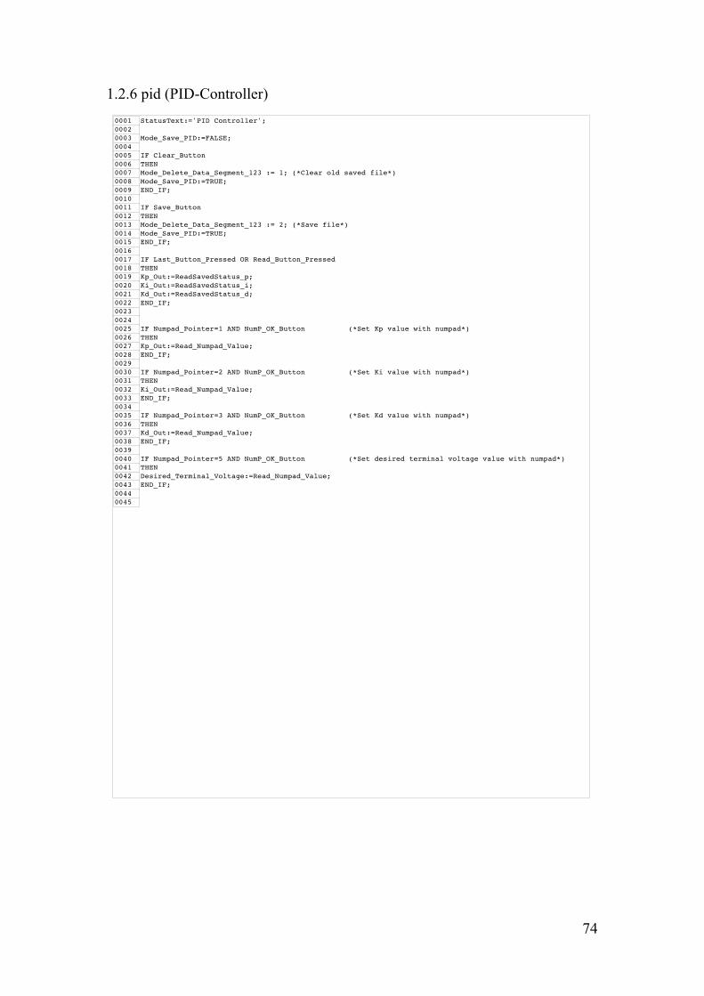
74

1.2.6 pid (PID-Controller)

0001 StatusText:='PID Controller';00020003 Mode_Save_PID:=FALSE;00040005 IF Clear_Button0006 THEN0007 Mode_Delete_Data_Segment_123 := 1; (*Clear old saved file*)0008 Mode_Save_PID:=TRUE;0009 END_IF;00100011 IF Save_Button0012 THEN0013 Mode_Delete_Data_Segment_123 := 2; (*Save file*)0014 Mode_Save_PID:=TRUE;0015 END_IF;00160017 IF Last_Button_Pressed OR Read_Button_Pressed0018 THEN0019 Kp_Out:=ReadSavedStatus_p;0020 Ki_Out:=ReadSavedStatus_i;0021 Kd_Out:=ReadSavedStatus_d;0022 END_IF;002300240025 IF Numpad_Pointer=1 AND NumP_OK_Button (*Set Kp value with numpad*)0026 THEN0027 Kp_Out:=Read_Numpad_Value;0028 END_IF;00290030 IF Numpad_Pointer=2 AND NumP_OK_Button (*Set Ki value with numpad*)0031 THEN0032 Ki_Out:=Read_Numpad_Value;0033 END_IF;00340035 IF Numpad_Pointer=3 AND NumP_OK_Button (*Set Kd value with numpad*)0036 THEN0037 Kd_Out:=Read_Numpad_Value;0038 END_IF;00390040 IF Numpad_Pointer=5 AND NumP_OK_Button (*Set desired terminal voltage value with numpad*)0041 THEN0042 Desired_Terminal_Voltage:=Read_Numpad_Value;0043 END_IF;00440045

75

1.2.7 if (Manual Field Current Control)

0001 (*StatusText:='Manual Field Current Controller';*)000200030004 IF Numpad_Pointer=4 AND NumP_OK_Button (*Set the If value with numpad*)0005 THEN0006 var_Manual_If:=Read_Numpad_Value;0007 END_IF;00080009 var_Manual_If:=var_Manual_If_slider*54;

76

1.2.8 auto

00010002 Mode_Open_Read_close_12345 := 5;0003 Mode_Read_PID:=TRUE;00040005 Kp_Out:=ReadSavedStatus_p;0006 Ki_Out:=ReadSavedStatus_i;0007 Kd_Out:=ReadSavedStatus_d;

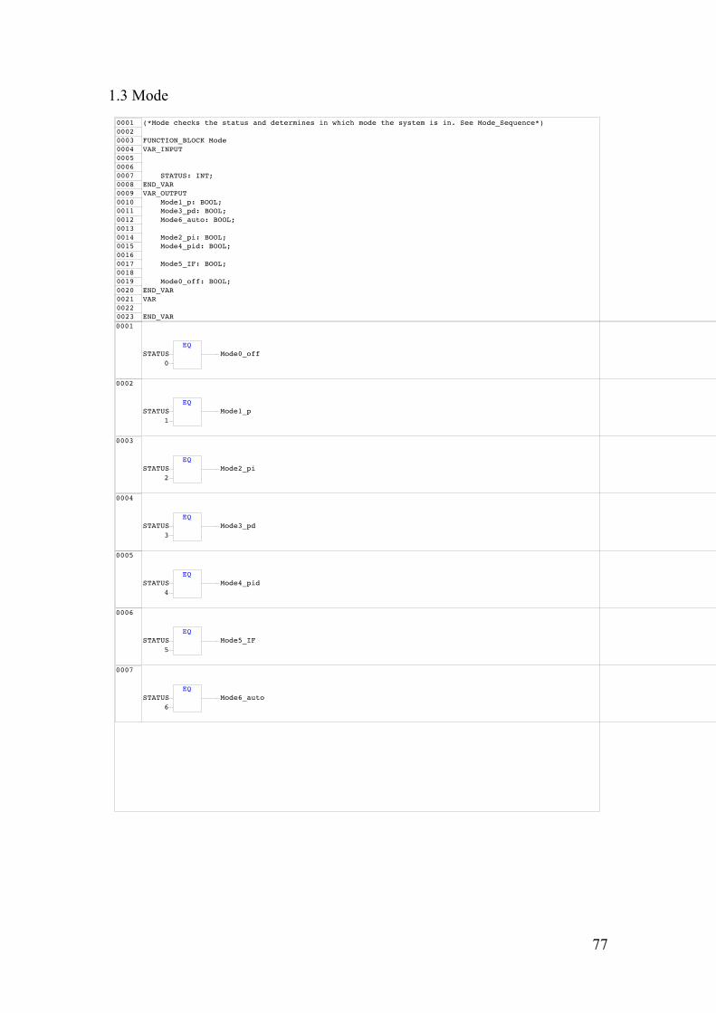
77

1.3 Mode

0001 (*Mode checks the status and determines in which mode the system is in. See Mode_Sequence*)00020003 FUNCTION_BLOCK Mode0004 VAR_INPUT000500060007 STATUS: INT;0008 END_VAR0009 VAR_OUTPUT0010 Mode1_p: BOOL;0011 Mode3_pd: BOOL;0012 Mode6_auto: BOOL;00130014 Mode2_pi: BOOL;0015 Mode4_pid: BOOL;00160017 Mode5_IF: BOOL;00180019 Mode0_off: BOOL;0020 END_VAR0021 VAR00220023 END_VAR0001

Mode0_offEQ

STATUS0

0002

Mode1_pEQ

STATUS1

0003

Mode2_piEQ

STATUS2

0004

Mode3_pdEQ

STATUS3

0005

Mode4_pidEQ

STATUS4

0006

Mode5_IFEQ

STATUS5

0007

Mode6_autoEQ

STATUS6

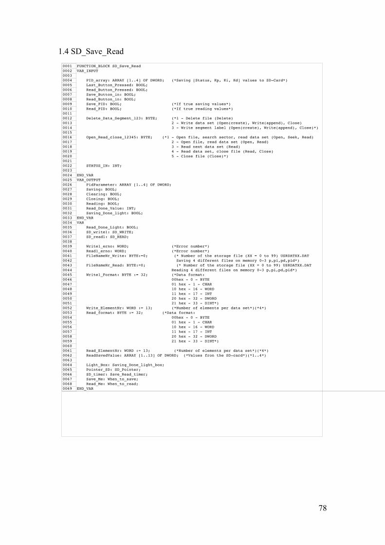
78

1.4 SD_Save_Read

0001 FUNCTION_BLOCK SD_Save_Read0002 VAR_INPUT00030004 PID_array: ARRAY [1..4] OF DWORD; (*Saving [Status, Kp, Ki, Kd] values to SD-Card*)0005 Last_Button_Pressed: BOOL;0006 Read_Button_Pressed: BOOL;0007 Save_Button_in: BOOL;0008 Read_Button_in: BOOL;0009 Save_PID: BOOL; (*If true saving values*)0010 Read_PID: BOOL; (*If true reading values*)00110012 Delete_Data_Segment_123: BYTE; (*1 - Delete file (Delete)0013 2 - Write data set (Open(create), Write(append), Close)0014 3 - Write segment label (Open(create), Write(append), Close)*)00150016 Open_Read_close_12345: BYTE; (*1 - Open file, search sector, read data set (Open, Seek, Read)0017 2 - Open file, read data set (Open, Read)0018 3 - Read next data set (Read)0019 4 - Read data set, close file (Read, Close)0020 5 - Close file (Close)*)00210022 STATUS_IN: INT;00230024 END_VAR0025 VAR_OUTPUT0026 PidParameter: ARRAY [1..4] OF DWORD;0027 Saving: BOOL;0028 Clearing: BOOL;0029 Closing: BOOL;0030 Reading: BOOL;0031 Read_Done_Value: INT;0032 Saving_Done_light: BOOL;0033 END_VAR0034 VAR0035 Read_Done_Light: BOOL;0036 SD_write1: SD_WRITE;0037 SD_read1: SD_READ;00380039 Write1_erno: WORD; (*Error number*)0040 Read1_erno: WORD; (*Error number*)0041 FileNameNr_Write: BYTE:=0; (* Number of the storage file (XX = 0 to 99) USRDATXX.DAT0042 Saving 4 different files on memory 0-3 p,pi,pd,pid*)0043 FileNameNr_Read: BYTE:=0; (* Number of the storage file (XX = 0 to 99) USRDATXX.DAT0044 Reading 4 different files on memory 0-3 p,pi,pd,pid*)0045 Write1_Format: BYTE := 32; (*Data format:0046 00hex - 0 - BYTE0047 01 hex - 1 - CHAR0048 10 hex - 16 - WORD0049 11 hex - 17 - INT0050 20 hex - 32 - DWORD0051 21 hex - 33 - DINT*)0052 Write_ElementNr: WORD := 13; (*Number of elements per data set*)(*4*)0053 Read_format: BYTE := 32; (*Data format:0054 00hex - 0 - BYTE0055 01 hex - 1 - CHAR0056 10 hex - 16 - WORD0057 11 hex - 17 - INT0058 20 hex - 32 - DWORD0059 21 hex - 33 - DINT*)00600061 Read_ElementNr: WORD := 13; (*Number of elements per data set*)(*4*)0062 ReadSavedValue: ARRAY [1..13] OF DWORD; (*Values fron the SD-card*)(*1..4*)00630064 Light_Box: Saving_Done_light_box;0065 Pointer_SD: SD_Pointer;0066 SD_timer: Save_Read_timer;0067 Save_Me: When_to_save;0068 Read_Me: When_to_read;0069 END_VAR

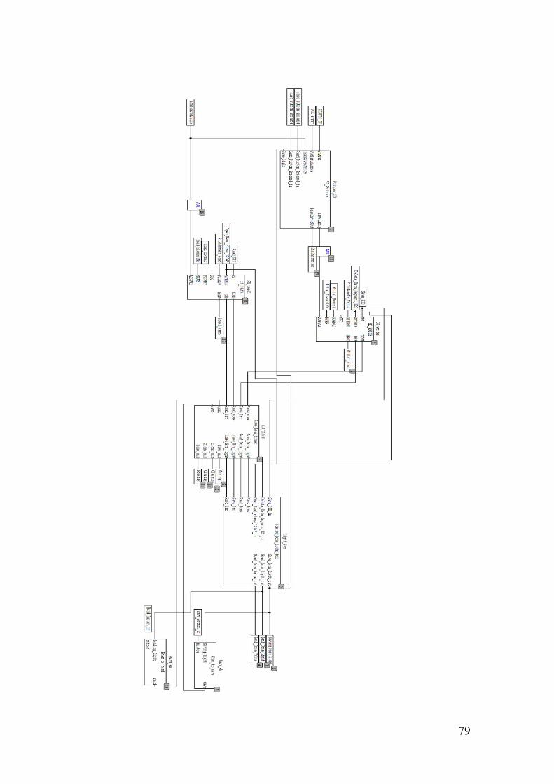
79

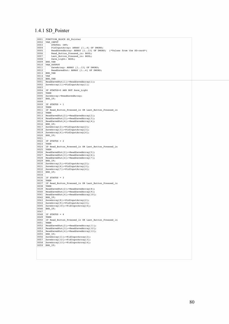
80

1.4.1 SD_Pointer

0001 FUNCTION_BLOCK SD_Pointer0002 VAR_INPUT0003 STATUS: INT;0004 PidInputArray: ARRAY [1..4] OF DWORD;0005 ReadSavedArray: ARRAY [1..13] OF DWORD; (*Values from the SD-card*)0006 Read_Button_Pressed_in: BOOL;0007 Last_Button_Pressed_in: BOOL;0008 Save_Light: BOOL;0009 END_VAR0010 VAR_OUTPUT0011 SaveArray: ARRAY [1..13] OF DWORD;0012 ReadSavedOut: ARRAY [1..4] OF DWORD;0013 END_VAR0014 VAR0015 END_VAR0001 ReadSavedOut[1]:=ReadSavedArray[1];0002 SaveArray[1]:=PidInputArray[1];00030004 IF STATUS=0 AND NOT Save_Light0005 THEN0006 SaveArray:=ReadSavedArray;0007 END_IF;00080009 IF STATUS = 10010 THEN0011 IF Read_Button_Pressed_in OR Last_Button_Pressed_in0012 THEN0013 ReadSavedOut[2]:=ReadSavedArray[2];0014 ReadSavedOut[3]:=ReadSavedArray[3];0015 ReadSavedOut[4]:=ReadSavedArray[4];0016 END_IF;0017 SaveArray[2]:=PidInputArray[2];0018 SaveArray[3]:=PidInputArray[3];0019 SaveArray[4]:=PidInputArray[4];0020 END_IF;00210022 IF STATUS = 20023 THEN0024 IF Read_Button_Pressed_in OR Last_Button_Pressed_in0025 THEN0026 ReadSavedOut[2]:=ReadSavedArray[5];0027 ReadSavedOut[3]:=ReadSavedArray[6];0028 ReadSavedOut[4]:=ReadSavedArray[7];0029 END_IF;0030 SaveArray[5]:=PidInputArray[2];0031 SaveArray[6]:=PidInputArray[3];0032 SaveArray[7]:=PidInputArray[4];0033 END_IF;00340035 IF STATUS = 30036 THEN0037 IF Read_Button_Pressed_in OR Last_Button_Pressed_in0038 THEN0039 ReadSavedOut[2]:=ReadSavedArray[8];0040 ReadSavedOut[3]:=ReadSavedArray[9];0041 ReadSavedOut[4]:=ReadSavedArray[10];0042 END_IF;0043 SaveArray[8]:=PidInputArray[2];0044 SaveArray[9]:=PidInputArray[3];0045 SaveArray[10]:=PidInputArray[4];0046 END_IF;00470048 IF STATUS = 40049 THEN0050 IF Read_Button_Pressed_in OR Last_Button_Pressed_in0051 THEN0052 ReadSavedOut[2]:=ReadSavedArray[11];0053 ReadSavedOut[3]:=ReadSavedArray[12];0054 ReadSavedOut[4]:=ReadSavedArray[13];0055 END_IF;0056 SaveArray[11]:=PidInputArray[2];0057 SaveArray[12]:=PidInputArray[3];0058 SaveArray[13]:=PidInputArray[4];0059 END_IF;

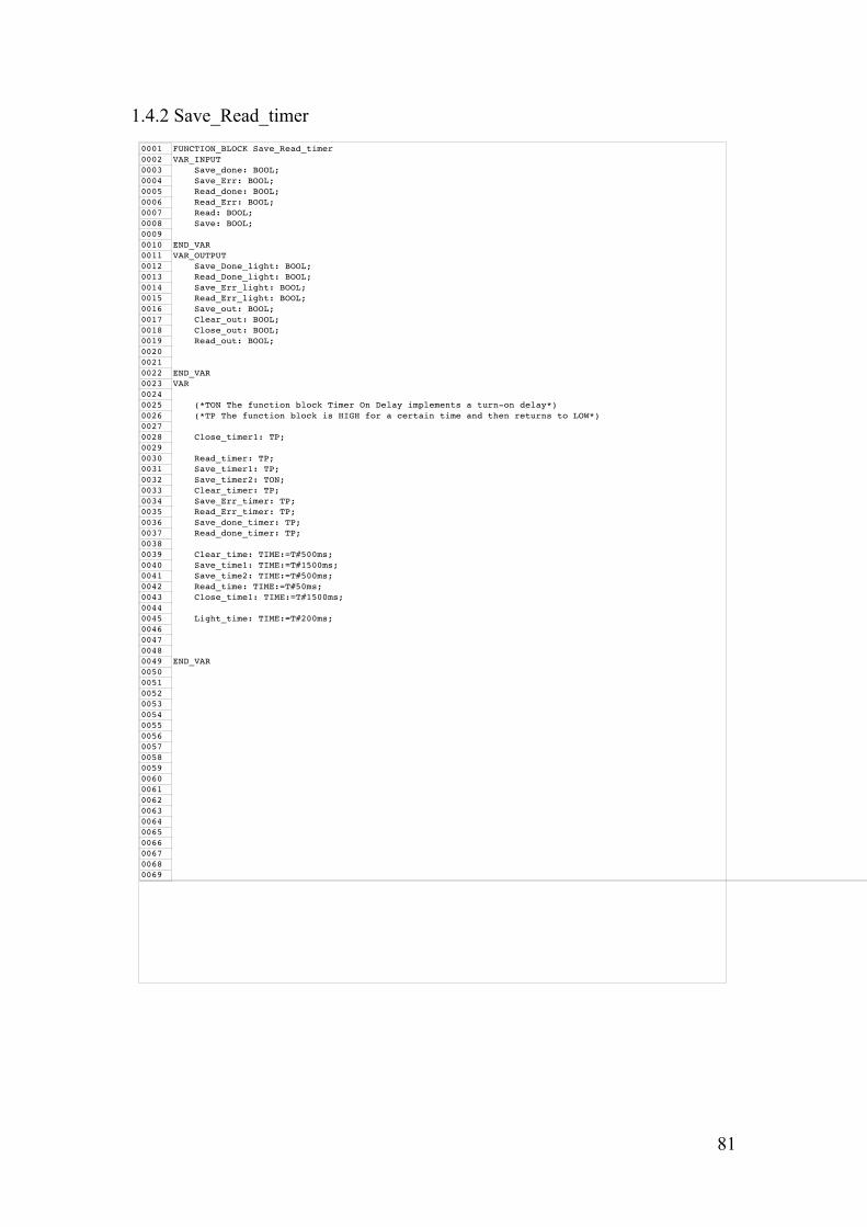
81

1.4.2 Save_Read_timer

0001 FUNCTION_BLOCK Save_Read_timer0002 VAR_INPUT0003 Save_done: BOOL;0004 Save_Err: BOOL;0005 Read_done: BOOL;0006 Read_Err: BOOL;0007 Read: BOOL;0008 Save: BOOL;00090010 END_VAR0011 VAR_OUTPUT0012 Save_Done_light: BOOL;0013 Read_Done_light: BOOL;0014 Save_Err_light: BOOL;0015 Read_Err_light: BOOL;0016 Save_out: BOOL;0017 Clear_out: BOOL;0018 Close_out: BOOL;0019 Read_out: BOOL;002000210022 END_VAR0023 VAR00240025 (*TON The function block Timer On Delay implements a turn-on delay*)0026 (*TP The function block is HIGH for a certain time and then returns to LOW*)00270028 Close_timer1: TP;00290030 Read_timer: TP;0031 Save_timer1: TP;0032 Save_timer2: TON;0033 Clear_timer: TP;0034 Save_Err_timer: TP;0035 Read_Err_timer: TP;0036 Save_done_timer: TP;0037 Read_done_timer: TP;00380039 Clear_time: TIME:=T#500ms;0040 Save_time1: TIME:=T#1500ms;0041 Save_time2: TIME:=T#500ms;0042 Read_time: TIME:=T#50ms;0043 Close_time1: TIME:=T#1500ms;00440045 Light_time: TIME:=T#200ms;0046004700480049 END_VAR00500051005200530054005500560057005800590060006100620063006400650066006700680069

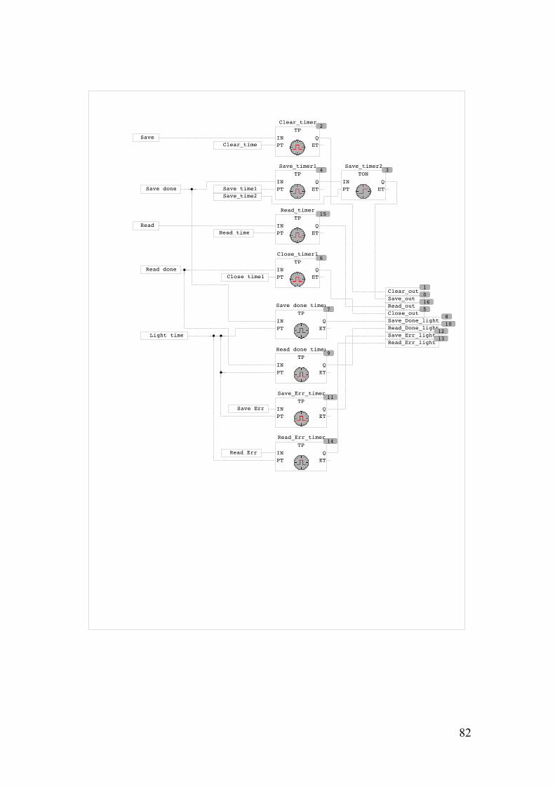
82

Save_out 0

Save_time1

Save

Clear_out 1

Clear_time

Close_time1

2 Clear_timerTP

INPT

QET

3 Save_timer2TON

INPT

QET

Save_time2Save_done

4 Save_timer1TP

INPT

QET

Close_out 5

Read_done

6 Close_timer1TP

INPT

QET

7 Save_done_timerTP

INPT

QET

Save_Done_light 8

9 Read_done_timerTP

INPT

QET

Read_Done_light 10

Save_Err

11 Save_Err_timerTP

INPT

QET

Save_Err_light 12 Light_time

Read_Err

Read_Err_light 13

14 Read_Err_timerTP

INPT

QET

Read_time

15 Read_timerTP

INPT

QET

Read_out 16

Read

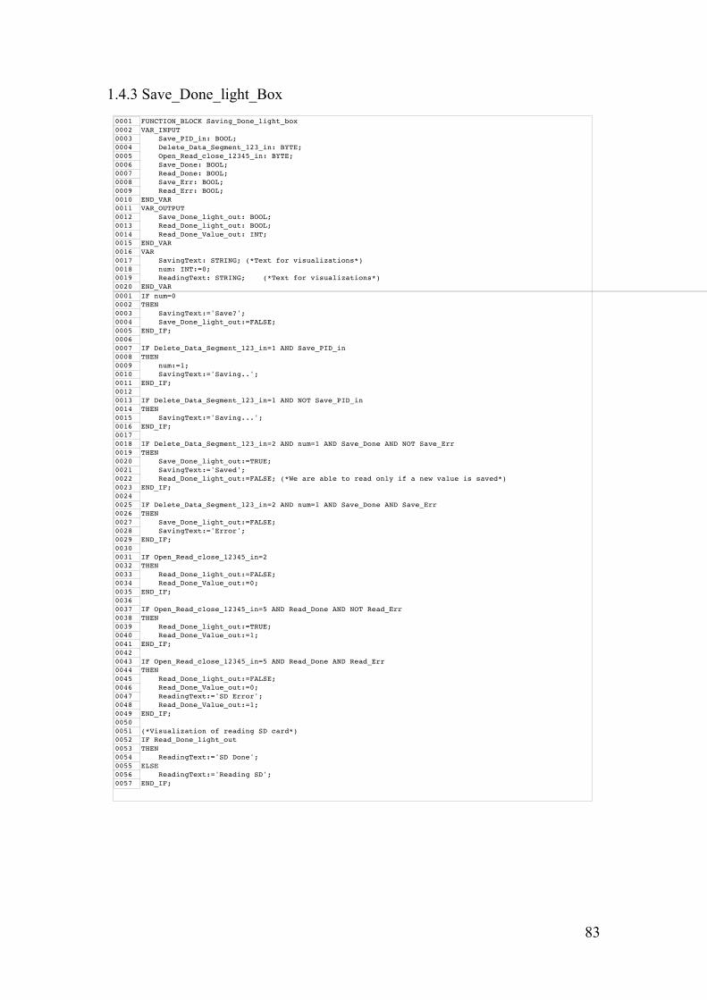
83

1.4.3 Save_Done_light_Box

0001 FUNCTION_BLOCK Saving_Done_light_box0002 VAR_INPUT0003 Save_PID_in: BOOL;0004 Delete_Data_Segment_123_in: BYTE;0005 Open_Read_close_12345_in: BYTE;0006 Save_Done: BOOL;0007 Read_Done: BOOL;0008 Save_Err: BOOL;0009 Read_Err: BOOL;0010 END_VAR0011 VAR_OUTPUT0012 Save_Done_light_out: BOOL;0013 Read_Done_light_out: BOOL;0014 Read_Done_Value_out: INT;0015 END_VAR0016 VAR0017 SavingText: STRING; (*Text for visualizations*)0018 num: INT:=0;0019 ReadingText: STRING; (*Text for visualizations*)0020 END_VAR0001 IF num=00002 THEN0003 SavingText:='Save?';0004 Save_Done_light_out:=FALSE;0005 END_IF;00060007 IF Delete_Data_Segment_123_in=1 AND Save_PID_in0008 THEN0009 num:=1;0010 SavingText:='Saving..';0011 END_IF;00120013 IF Delete_Data_Segment_123_in=1 AND NOT Save_PID_in0014 THEN0015 SavingText:='Saving...';0016 END_IF;00170018 IF Delete_Data_Segment_123_in=2 AND num=1 AND Save_Done AND NOT Save_Err0019 THEN0020 Save_Done_light_out:=TRUE;0021 SavingText:='Saved';0022 Read_Done_light_out:=FALSE; (*We are able to read only if a new value is saved*)0023 END_IF;00240025 IF Delete_Data_Segment_123_in=2 AND num=1 AND Save_Done AND Save_Err0026 THEN0027 Save_Done_light_out:=FALSE;0028 SavingText:='Error';0029 END_IF;00300031 IF Open_Read_close_12345_in=20032 THEN0033 Read_Done_light_out:=FALSE;0034 Read_Done_Value_out:=0;0035 END_IF;00360037 IF Open_Read_close_12345_in=5 AND Read_Done AND NOT Read_Err0038 THEN0039 Read_Done_light_out:=TRUE;0040 Read_Done_Value_out:=1;0041 END_IF;00420043 IF Open_Read_close_12345_in=5 AND Read_Done AND Read_Err0044 THEN0045 Read_Done_light_out:=FALSE;0046 Read_Done_Value_out:=0;0047 ReadingText:='SD Error';0048 Read_Done_Value_out:=1;0049 END_IF;00500051 (*Visualization of reading SD card*)0052 IF Read_Done_light_out0053 THEN0054 ReadingText:='SD Done';0055 ELSE0056 ReadingText:='Reading SD';0057 END_IF;

84

1.4.4 When_to_save

0001 FUNCTION_BLOCK When_to_save0002 VAR_INPUT0003 Saving_light: BOOL;0004 button: BOOL;0005 END_VAR0006 VAR_OUTPUT0007 save: BOOL;0008 END_VAR0009 VAR0010 END_VAR0001 IF Saving_light0002 THEN0003 save:=FALSE;0004 ELSE0005 save:=button;0006 END_IF;

85

1.4.5 When_to_read

0001 FUNCTION_BLOCK When_to_read0002 VAR_INPUT0003 Reading_light: BOOL;0004 button: BOOL;0005 END_VAR0006 VAR_OUTPUT0007 read: BOOL;0008 END_VAR0009 VAR0010 END_VAR0001 IF Reading_light0002 THEN0003 read:=FALSE;0004 ELSE0005 read:=button;0006 END_IF;0007

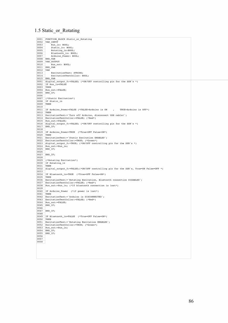
86

1.5 Static_or_Rotating

0001 FUNCTION_BLOCK Static_or_Rotating0002 VAR_INPUT0003 Run_in: BOOL;0004 Static_in: BOOL;0005 Rotating_in:BOOL;0006 Bluetooth_in: BOOL;0007 Arduino_Power: BOOL;0008 END_VAR0009 VAR_OUTPUT0010 Run_out: BOOL;0011 END_VAR0012 VAR0013 ExcitationText: STRING;0014 ExcitationTextCollor: BOOL;0015 END_VAR0001 digital_output_0:=FALSE; (*ON/OFF controlling pin for the SSR's *)0002 IF Run_in=FALSE0003 THEN0004 Run_out:=FALSE;0005 END_IF;00060007 (*Static Excitation*)0008 IF Static_in0009 THEN00100011 IF Arduino_Power=FALSE (*FALSE=Arduino is ON , TRUE=Arduino is OFF*)0012 THEN0013 ExcitationText:='Turn off Arduino, disconnect USB cable!';0014 ExcitationTextCollor:=FALSE; (*Red*)0015 Run_out:=FALSE;0016 digital_output_0:=FALSE; (*ON/OFF controlling pin for the SSR's *)0017 END_IF;00180019 IF Arduino_Power=TRUE (*True=OFF False=ON*)0020 THEN0021 ExcitationText:='Static Excitation ENABLED';0022 ExcitationTextCollor:=TRUE; (*Green*)0023 digital_output_0:=TRUE; (*ON/OFF controlling pin for the SSR's *)0024 Run_out:=Run_in;0025 END_IF;00260027 END_IF;00280029 (*Rotating Excitation*)0030 IF Rotating_in0031 THEN0032 digital_output_0:=FALSE;(*ON/OFF controlling pin for the SSR's, True=ON False=OFF *)00330034 IF Bluetooth_in=TRUE (*True=OFF False=ON*)0035 THEN0036 ExcitationText:='Rotating Excitation, Bluetooth connection DISABLED';0037 ExcitationTextCollor:=FALSE; (*Red*)0038 Run_out:=Run_in; (*If bluetooth connection is lost*)00390040 IF Arduino_Power (*if power is lost*)0041 THEN0042 ExcitationText:='Arduino is DISCONNECTED';0043 ExcitationTextCollor:=FALSE; (*Red*)0044 Run_out:=FALSE;0045 END_IF;00460047 END_IF;00480049 IF Bluetooth_in=FALSE (*True=OFF False=ON*)0050 THEN0051 ExcitationText:='Rotating Excitation ENABLED';0052 ExcitationTextCollor:=TRUE; (*Green*)0053 Run_out:=Run_in;0054 END_IF;0055 END_IF;005600570058

87

1.6 KiKd_to_TnTv

0001 (*Converts the Ki and Kd parameters to Tn and Tv so that they are compatible with the regulators*)0002 FUNCTION_BLOCK KiKd_to_TnTv0003 VAR_INPUT0004 Kp_in: REAL;0005 Ki: REAL;0006 Kd: REAL;0007 END_VAR0008 VAR_OUTPUT0009 Kp_out: REAL;0010 Tn: REAL;0011 Tv: REAL;0012 END_VAR0013 VAR0014 END_VAR0001 Kp_out:=Kp_in;0002 Tn:=Kp_in/Ki;0003 Tv:=Kd/Kp_in;0004

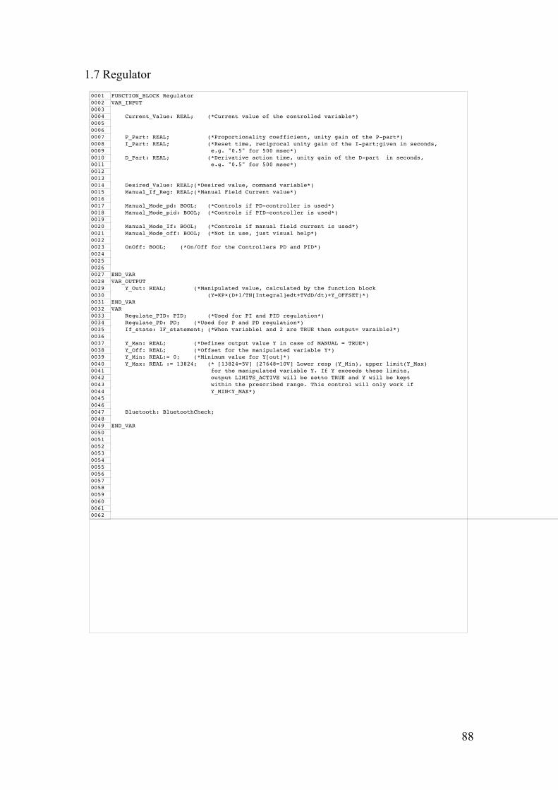
88

1.7 Regulator

0001 FUNCTION_BLOCK Regulator0002 VAR_INPUT00030004 Current_Value: REAL; (*Current value of the controlled variable*)000500060007 P_Part: REAL; (*Proportionality coefficient, unity gain of the P-part*)0008 I_Part: REAL; (*Reset time, reciprocal unity gain of the I-part;given in seconds,0009 e.g. "0.5" for 500 msec*)0010 D_Part: REAL; (*Derivative action time, unity gain of the D-part in seconds,0011 e.g. "0.5" for 500 msec*)001200130014 Desired_Value: REAL;(*Desired value, command variable*)0015 Manual_If_Reg: REAL;(*Manual Field Current value*)00160017 Manual_Mode_pd: BOOL; (*Controls if PD-controller is used*)0018 Manual_Mode_pid: BOOL; (*Controls if PID-controller is used*)00190020 Manual_Mode_If: BOOL; (*Controls if manual field current is used*)0021 Manual_Mode_off: BOOL; (*Not in use, just visual help*)00220023 OnOff: BOOL; (*On/Off for the Controllers PD and PID*)0024002500260027 END_VAR0028 VAR_OUTPUT0029 Y_Out: REAL; (*Manipulated value, calculated by the function block0030 (Y=KP×(D+1/TN[Integral]edt+TVdD/dt)+Y_OFFSET)*)0031 END_VAR0032 VAR0033 Regulate_PID: PID; (*Used for PI and PID regulation*)0034 Regulate_PD: PD; (*Used for P and PD regulation*)0035 If_state: IF_statement; (*When variable1 and 2 are TRUE then output= varaible3*)00360037 Y_Man: REAL; (*Defines output value Y in case of MANUAL = TRUE*)0038 Y_Off: REAL; (*Offset for the manipulated variable Y*)0039 Y_Min: REAL:= 0; (*Minimum value for Y[out]*)0040 Y_Max: REAL := 13824; (* [13824=5V] [27648=10V] Lower resp (Y_Min), upper limit(Y_Max)0041 for the manipulated variable Y. If Y exceeds these limits,0042 output LIMITS_ACTIVE will be setto TRUE and Y will be kept0043 within the prescribed range. This control will only work if0044 Y_MIN<Y_MAX*)004500460047 Bluetooth: BluetoothCheck;00480049 END_VAR0050005100520053005400550056005700580059006000610062

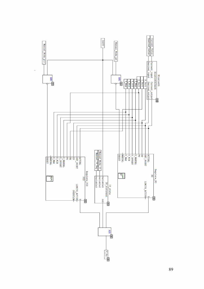
89

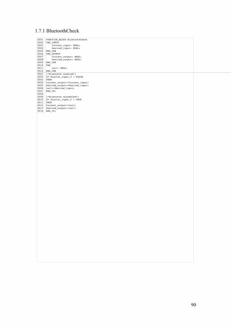
90

1.7.1 BluetoothCheck

0001 FUNCTION_BLOCK BluetoothCheck0002 VAR_INPUT0003 Current_input: REAL;0004 Desired_input: REAL;0005 END_VAR0006 VAR_OUTPUT0007 Current_output: REAL;0008 Desired_output: REAL;0009 END_VAR0010 VAR0011 var1: REAL;0012 END_VAR0001 (*Bluetooth enabled*)0002 IF digital_input_0 = FALSE0003 THEN0004 Current_output:=Current_input;0005 Desired_output:=Desired_input;0006 var1:=Desired_input;0007 END_IF;00080009 (*Bluetooth dissabled*)0010 IF digital_input_0 = TRUE0011 THEN0012 Current_output:=var1;0013 Desired_output:=var1;0014 END_IF;

91

1.7.2 IF_Statement

0001 (*IF_statement controlls the manual control of the field current*)00020003 FUNCTION_BLOCK IF_statement0004 VAR_INPUT0005 variable1: BOOL; (*OnOff*)0006 variable2: BOOL; (*Manual_Mode_If*)0007 variable3: REAL; (*Manual_If_Reg*)0008 END_VAR0009 VAR_OUTPUT0010 out: REAL; (*Output value*)0011 END_VAR0012 VAR00130014 END_VAR0001 out := 0;00020003 IF variable1 AND variable20004 THEN0005 out := variable3;00060007 IF variable3>13824 (*13824 = 5V = Arduino maximum*)0008 THEN0009 out:=13824;00100011 END_IF;0012 END_IF;0013

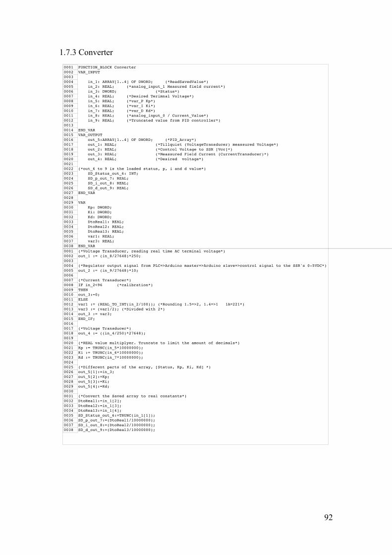
92

1.7.3 Converter

0001 FUNCTION_BLOCK Converter0002 VAR_INPUT00030004 in_1: ARRAY[1..4] OF DWORD; (*ReadSavedValue*)0005 in_2: REAL; (*analog_input_1 Measured field current*)0006 in_3: DWORD; (*Status*)0007 in_4: REAL; (*Desired Terimnal Voltage*)0008 in_5: REAL; (*var_P Kp*)0009 in_6: REAL; (*var_I Ki*)0010 in_7: REAL; (*var_D Kd*)0011 in_8: REAL; (*analog_input_0 / Current_Value*)0012 in_9: REAL; (*Truncated value from PID controller*)00130014 END_VAR0015 VAR_OUTPUT0016 out_5:ARRAY[1..4] OF DWORD; (*PID_Array*)0017 out_1: REAL; (*Tillquist (VoltageTransducer) meassured Voltage*)0018 out_2: REAL; (*Control Voltage to SSR [Vcc]*)0019 out_3: REAL; (*Meassured Field Current (CurrentTransducer)*)0020 out_4: REAL; (*Desired voltage*)00210022 (*out_6 to 9 is the loaded status, p, i and d value*)0023 SD_Status_out_6: INT;0024 SD_p_out_7: REAL;0025 SD_i_out_8: REAL;0026 SD_d_out_9: REAL;0027 END_VAR00280029 VAR0030 Kp: DWORD;0031 Ki: DWORD;0032 Kd: DWORD;0033 DtoReal1: REAL;0034 DtoReal2: REAL;0035 DtoReal3: REAL;0036 var1: REAL;0037 var3: REAL;0038 END_VAR0001 (*Voltage Transducer, reading real time AC terminal voltage*)0002 out_1 := (in_8/27648)*250;00030004 (*Regulator output signal from PLC=>Arduino master=>Arduino slave=>control signal to the SSR's 0-5VDC*)0005 out_2 := (in_9/27648)*10;00060007 (*Current Transducer*)0008 IF in_2<96 (*calibration*)0009 THEN0010 out_3:=0;0011 ELSE0012 var1 := (REAL_TO_INT(in_2/100)); (*Rounding 1.5=>2, 1.4=>1 1A=221*)0013 var3 := (var1/2); (*Divided with 2*)0014 out_3 := var3;0015 END_IF;00160017 (*Voltage Transducer*)0018 out_4 := ((in_4/250)*27648);00190020 (*REAL value multiplyer. Truncate to limit the amount of decimals*)0021 Kp := TRUNC(in_5*10000000);0022 Ki := TRUNC(in_6*10000000);0023 Kd := TRUNC(in_7*10000000);00240025 (*Different parts of the array, [Status, Kp, Ki, Kd] *)0026 out_5[1]:=in_3;0027 out_5[2]:=Kp;0028 out_5[3]:=Ki;0029 out_5[4]:=Kd;00300031 (*Convert the Saved array to real constants*)0032 DtoReal1:=in_1[2];0033 DtoReal2:=in_1[3];0034 DtoReal3:=in_1[4];0035 SD_Status_out_6:=TRUNC(in_1[1]);0036 SD_p_out_7:=(DtoReal1/10000000);0037 SD_i_out_8:=(DtoReal2/10000000);0038 SD_d_out_9:=(DtoReal3/10000000);

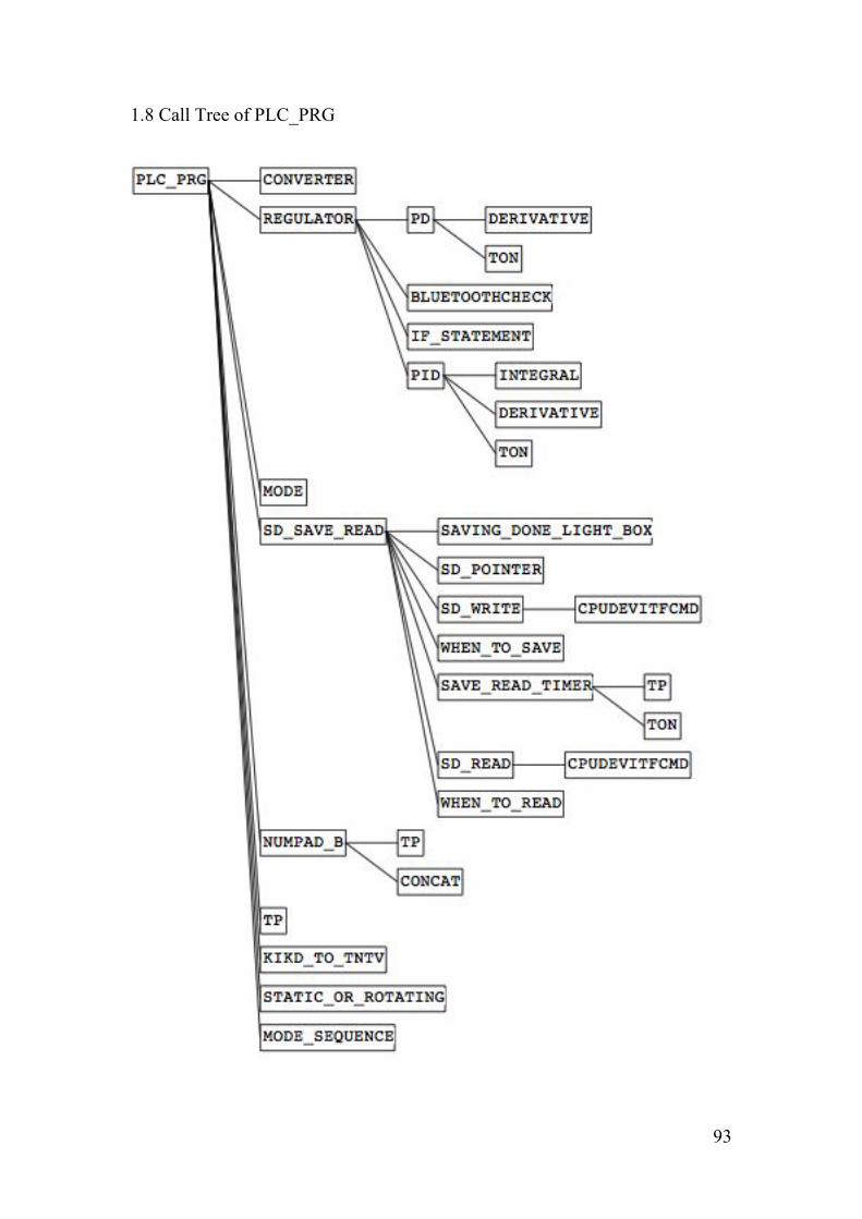
93

1.8 Call Tree of PLC_PRG

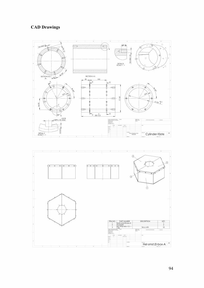
94

CAD Drawings

��[�����

�5���

�������

$

$

&

������������

�����

���� �����

'

' '

'

��[�����

� ���������� �

�5���

%

6(&7,21�$�$

���[����

���[�0�[�����

'(7$,/�%�6&$/(������

����3��������������������

����������

'(7$,/�&�6&$/(������

�������[�����

���[�0�[���� ���[����

6(&7,21�'�'�[

'

(

)

&

� � � �

%

$

��� �

&

'

� � � �

$

%

&\OLQGHU�IlVWH

����������7/-

:(,*+7��

5|U� �����[�����6���-�+

$�

6+((7���2)��6&$/(����

':*�12�

7,7/(�

5(9,6,21'2�127�6&$/(�'5$:,1*

0$7(5,$/�

'$7(6,*1$785(1$0(

'(%85�$1'�%5($.�6+$53�('*(6

),1,6+�81/(66�27+(5:,6(�63(&,),('�',0(16,216�$5(�,1�0,//,0(7(56685)$&(�),1,6+�72/(5$1&(6�/,1($5�-6���MV��',$0(7(5�-6���MV��

4�$

0)*

$339'

&+.'

'5$:1

�

�

�

�

,7(0�12� 3$57�180%(5 '(6&5,37,21 47<�� 6YHWV�VPVW�(O�ER[�$ �� gYHUSOnW �� ,62������0��[��������

��1 6NUXY�VWnO ��

'

(

)

&

� � � �

%

$

��� �

&

'

� � � �

$

%

+HO�VPVW�(O�ER[�$

����������7/-

:(,*+7��

$�

6+((7���2)��6&$/(����

':*�12�

7,7/(�

5(9,6,21'2�127�6&$/(�'5$:,1*

0$7(5,$/�

'$7(6,*1$785(1$0(

'(%85�$1'�%5($.�6+$53�('*(6

),1,6+�81/(66�27+(5:,6(�63(&,),('�',0(16,216�$5(�,1�0,//,0(7(56685)$&(�),1,6+�72/(5$1&(6�/,1($5�-6���MV��',$0(7(5�-6���MV��

4�$

0)*

$339'

&+.'

'5$:1

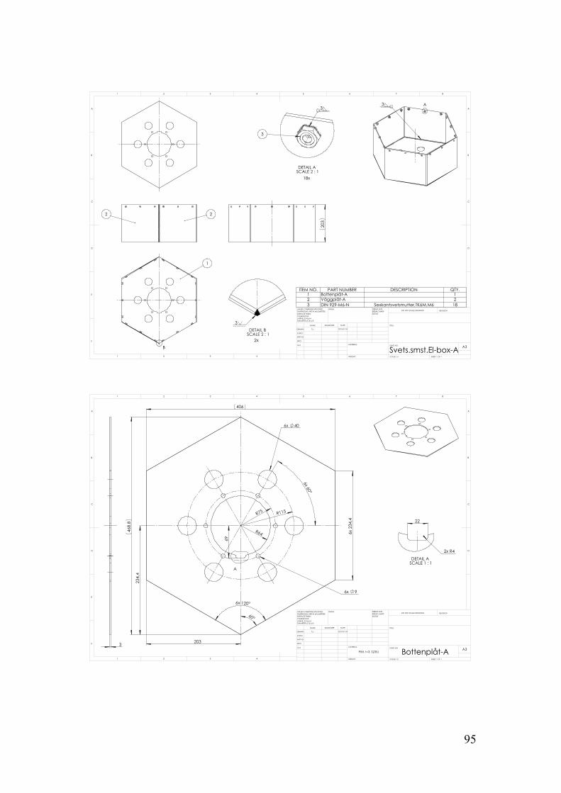
95

%

�

��

�����

$

�[

�

'(7$,/�$�6&$/(������

�

�

'(7$,/�%�6&$/(������

�

��[

,7(0�12� 3$57�180%(5 '(6&5,37,21 47<�� %RWWHQSOnW�$ �� 9lJJSOnW�$ �� ',1�����0��1 6H[NDQWVYHWVPXWWHU�7.�0�0� ��

'

(

)

&

� � � �

%

$

��� �

&

'

� � � �

$

%

6YHWV�VPVW�(O�ER[�$

����������7/-

:(,*+7��

$�

6+((7���2)��6&$/(����

':*�12�

7,7/(�

5(9,6,21'2�127�6&$/(�'5$:,1*

0$7(5,$/�

'$7(6,*1$785(1$0(

'(%85�$1'�%5($.�6+$53�('*(6

),1,6+�81/(66�27+(5:,6(�63(&,),('�',0(16,216�$5(�,1�0,//,0(7(56685)$&(�),1,6+�72/(5$1&(6�/,1($5�-6���MV��',$0(7(5�-6���MV��

4�$

0)*

$339'

&+.'

'5$:1

�����

��[������

��[�������

�������

�������

�5���

��[� ���

��[� ��

����

�����

�����

��[�����

�5��� �5����

$

���

����

��[�5��

'(7$,/�$�6&$/(������

'

(

)

&

� � � �

%

$

��� �

&

'

� � � �

$

%

%RWWHQSOnW�$

����������7/-

:(,*+7��

3OnW��W ���6���-$�

6+((7���2)��6&$/(����

':*�12�

7,7/(�

5(9,6,21'2�127�6&$/(�'5$:,1*

0$7(5,$/�

'$7(6,*1$785(1$0(

'(%85�$1'�%5($.�6+$53�('*(6

),1,6+�81/(66�27+(5:,6(�63(&,),('�',0(16,216�$5(�,1�0,//,0(7(56685)$&(�),1,6+�72/(5$1&(6�/,1($5�-6���MV��',$0(7(5�-6���MV��

4�$

0)*

$339'

&+.'

'5$:1

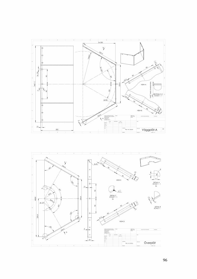
96

���

��[������

��[�5��

�5����

�����

�����

�������

�������

�������

��[�����

$

%

)

�����

�������

����

��[�

��

����

����& &

����

����

������

����

9,(:�$

������

����

���� ����

9,(:�%

�[��

�KHOD�|YHUNDQWHQ

�XWY����������������������������

6(&7,21�&�&�6&$/(������

'

(

)

&

� � � �

%

$

��� �

&

'

� � � �

$

%

9lJJSOnW�$

����������7/-

:(,*+7��

3OnW��W ���6���-5 $�

6+((7���2)��6&$/(����

':*�12�

7,7/(�

5(9,6,21'2�127�6&$/(�'5$:,1*

0$7(5,$/�

'$7(6,*1$785(1$0(

'(%85�$1'�%5($.�6+$53�('*(6

),1,6+�81/(66�27+(5:,6(�63(&,),('�',0(16,216�$5(�,1�0,//,0(7(56685)$&(�),1,6+�72/(5$1&(6�/,1($5�-6���MV��',$0(7(5�-6���MV��

4�$

0)*

$339'

&+.'

'5$:1

�5���

�����

�����

��[� ��

�������

�������

�������

�������

�������

�����

�����

������

������

�5���

$

%

&

'

(��[�5��

���

����

����

����

����

���

����

�5��

'(7$,/�$�6&$/(������

���

���

'(7$,/�%�6&$/(������

'(7$,/�&�6&$/(������

�

������

����

����

����

9,(:�'

�[

������

����

����

����

9,(:�(

�[

'

(

)

&

� � � �

%

$

��� �

&

'

� � � �

$

%

gYHUSOnW

����������7/-

:(,*+7��

3OnW��W ���6���-U$�

6+((7���2)��6&$/(����

':*�12�

7,7/(�

5(9,6,21'2�127�6&$/(�'5$:,1*

0$7(5,$/�

'$7(6,*1$785(1$0(

'(%85�$1'�%5($.�6+$53�('*(6

),1,6+�81/(66�27+(5:,6(�63(&,),('�',0(16,216�$5(�,1�0,//,0(7(56685)$&(�),1,6+�72/(5$1&(6�/,1($5�-6���MV��',$0(7(5�-6���MV��

4�$

0)*

$339'

&+.'

'5$:1

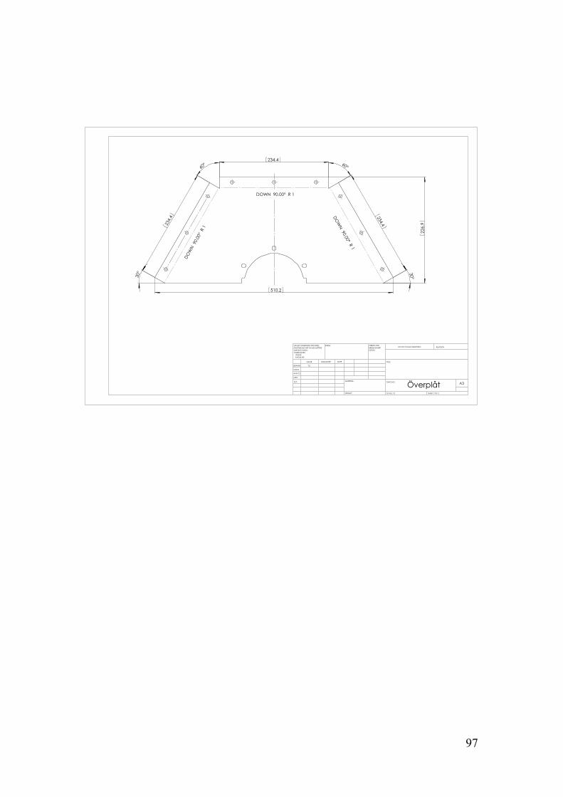
97

����� �����

����������

�������������� �������

�������

�������

'2:1����������5���

'2:1����������5���

'2:1����������5���

gYHUSOnW

7/-

:(,*+7��

$�

6+((7���2)��6&$/(����

':*�12�

7,7/(�

5(9,6,21'2�127�6&$/(�'5$:,1*

0$7(5,$/�

'$7(6,*1$785(1$0(

'(%85�$1'�%5($.�6+$53�('*(6

),1,6+�81/(66�27+(5:,6(�63(&,),('�',0(16,216�$5(�,1�0,//,0(7(56685)$&(�),1,6+�72/(5$1&(6����/,1($5����$1*8/$5�

4�$

0)*

$339'

&+.'

'5$:1