Embed Size (px)
Citation preview
Baseband Receiver
Unipolar vs. Polar SignalingSignal Space Representation

Unipolar vs. Polar Signaling
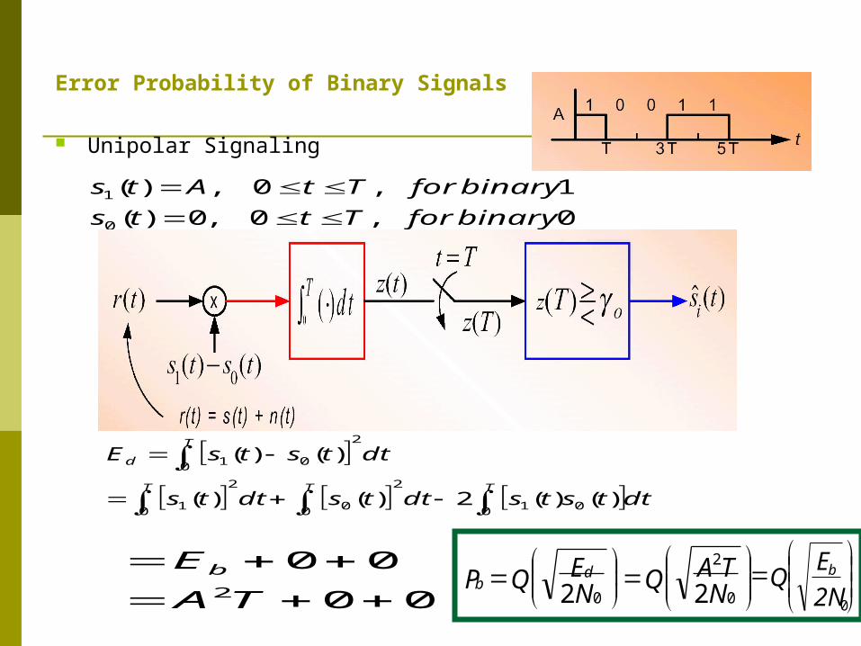
Error Probability of Binary Signals Unipolar Signaling
0,0,0)(
1,0,)(
0
1
binaryforTtts
binaryforTtAts
dttstsE
dttstsdttsdtts
dttstsE
T
b
TTT
T
d
0 01
0 01
2
0 0
2
0 1
2
0 01
)()(22
)()(2)()(
)()(
00
002
TA
Eb
0
2
0 22 NTAQN
EQP db
02N
EQ b
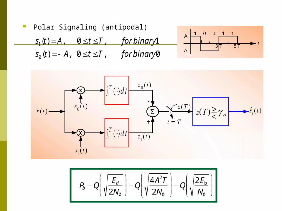
Polar Signaling (antipodal)
0,0,)(
1,0,)(
0
1
binaryforTtAts
binaryforTtAts
00
2
0
2
2
4
2 N
EQ
N
TAQ
N
EQP bd
b

Bipolar signals require a factor of 2 increase in energy compared to Orthagonal
Since 10log102 = 3 dB, we say that bipolar signaling offers a 3 dB better performance than Orthagonal
0
2
N
EQP b
b
0
)(
N
EQP
AntipodalBipolarOrthogonal
bb
6
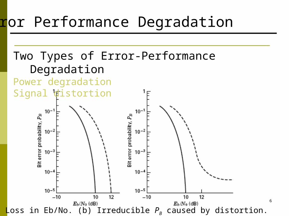
Error Performance Degradation
Two Types of Error-Performance DegradationPower degradationSignal distortion
(a) Loss in Eb/No. (b) Irreducible PB caused by distortion.
Signal Space Analysis
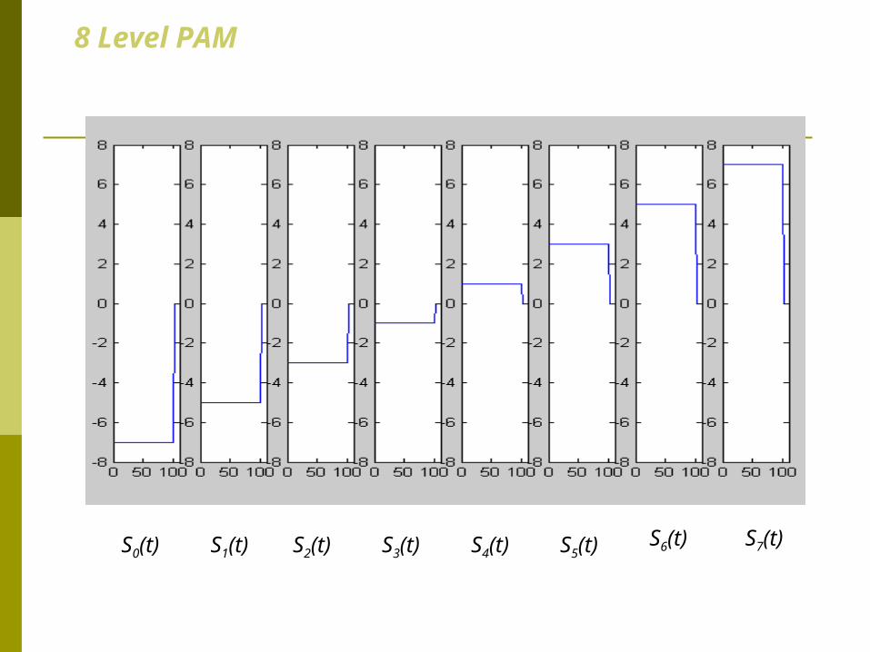
8 Level PAM
S0(t) S1(t) S2(t) S3(t) S4(t) S5(t)S6(t) S7(t)
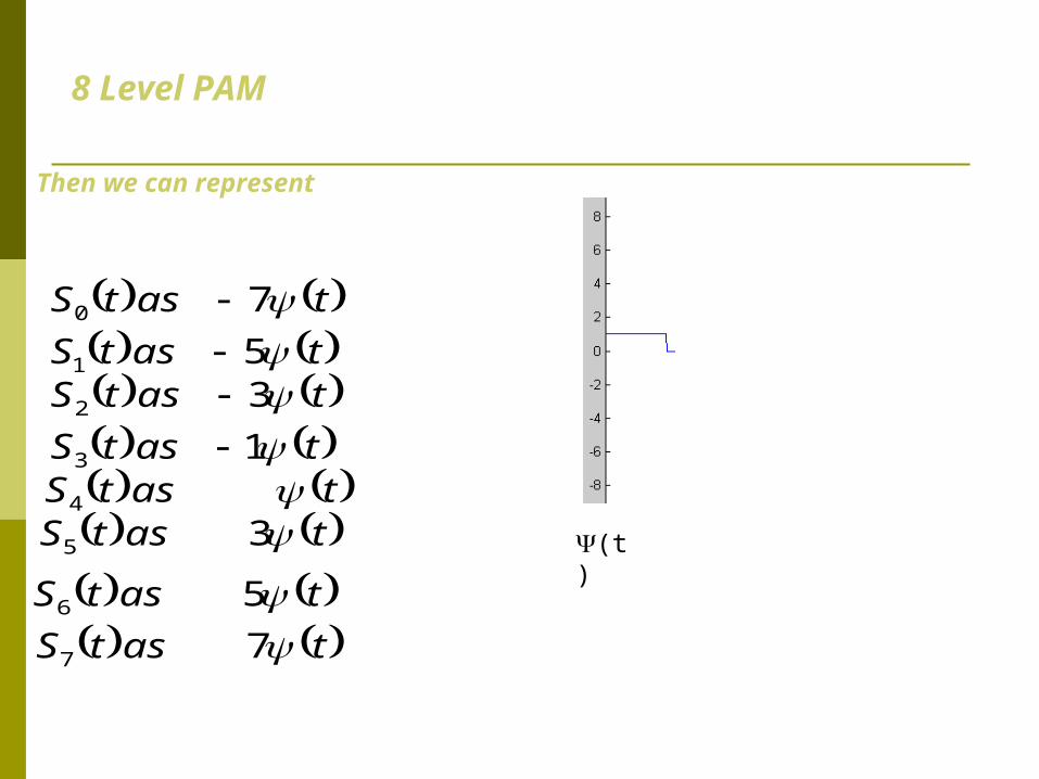
8 Level PAM
Then we can represent
(t)
tastS 4
tastS 35
tastS 56
tastS 77
tastS 13 tastS 32
tastS 70 tastS 51
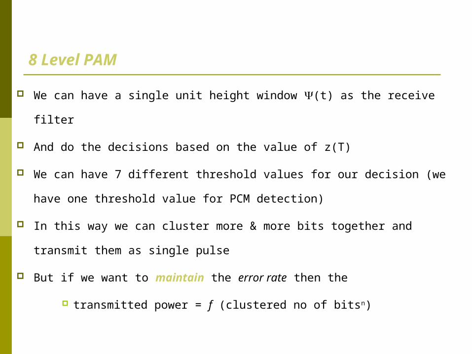
8 Level PAM
We can have a single unit height window (t) as the receive filter
And do the decisions based on the value of z(T)
We can have 7 different threshold values for our decision (we have one
threshold value for PCM detection)
In this way we can cluster more & more bits together and transmit them as
single pulse
But if we want to maintain the error rate then the
transmitted power = f (clustered no of bitsn)
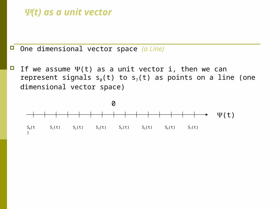
(t) as a unit vector
One dimensional vector space (a Line)
If we assume (t) as a unit vector i, then we can represent signals s0(t) to s7(t) as points on a line (one dimensional vector space)
S1(t) S2(t) S3(t) S4(t) S5(t) S6(t) S7(t)S0(t)
(t)
0
12
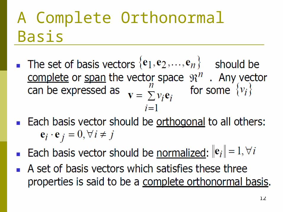
A Complete Orthonormal Basis

Signal space What is a signal space?
Vector representations of signals in an N-dimensional orthogonal space
Why do we need a signal space? It is a means to convert signals to vectors and vice
versa. It is a means to calculate signals energy and Euclidean
distances between signals. Why are we interested in Euclidean distances
between signals? For detection purposes: The received signal is
transformed to a received vectors. The signal which has the minimum distance to the received signal is estimated as the transmitted signal.
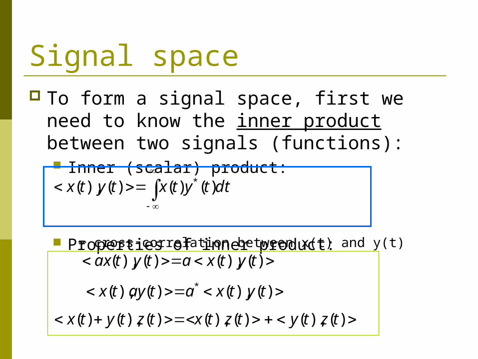
Signal space To form a signal space, first we need to
know the inner product between two signals (functions): Inner (scalar) product:
Properties of inner product:
dttytxtytx )()()(),( *
= cross-correlation between x(t) and y(t)
)(),()(),( tytxatytax
)(),()(),( * tytxataytx
)(),()(),()(),()( tztytztxtztytx
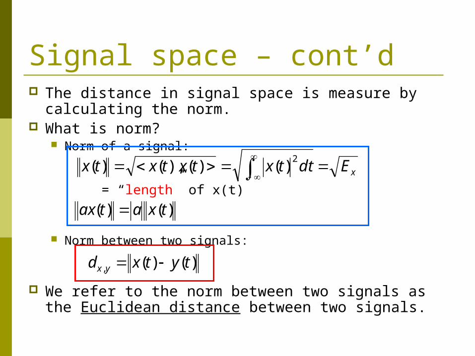
Signal space – cont’d The distance in signal space is measure by
calculating the norm. What is norm?
Norm of a signal:
Norm between two signals:
We refer to the norm between two signals as the Euclidean distance between two signals.
xEdttxtxtxtx
2)()(),()(
)()( txatax
)()(, tytxd yx
= “length” of x(t)
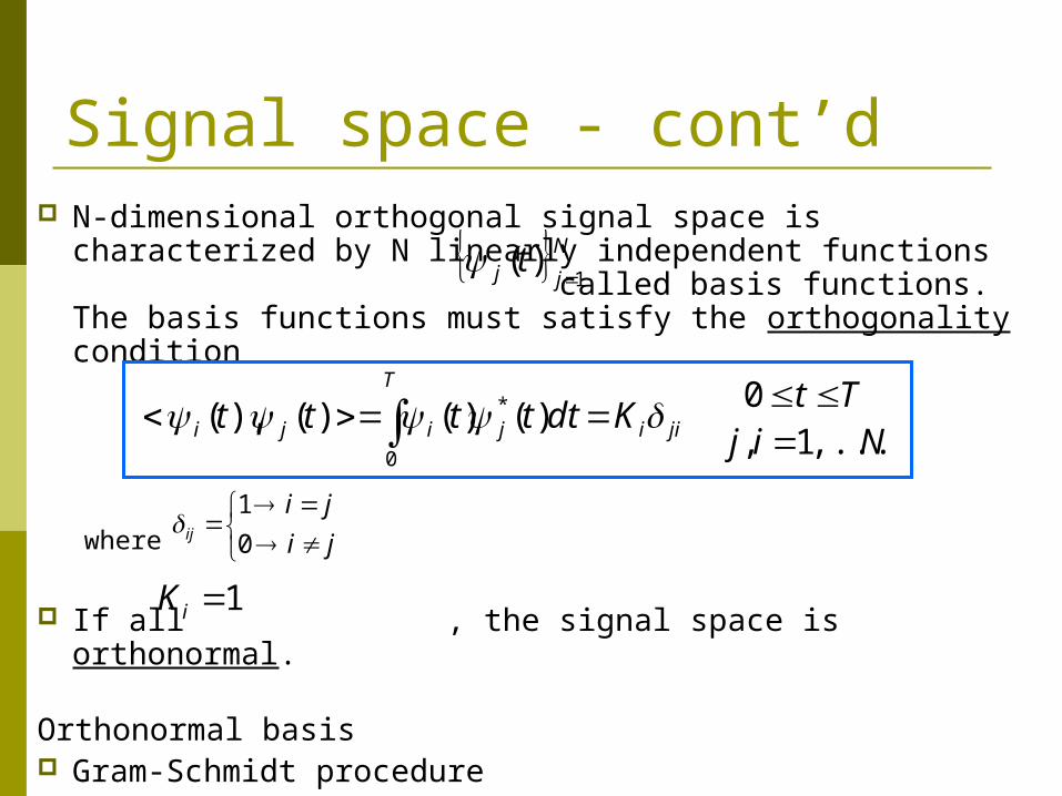
Signal space - cont’d N-dimensional orthogonal signal space is
characterized by N linearly independent functions called basis functions. The basis functions must satisfy the orthogonality condition
where
If all , the signal space is orthonormal.
Orthonormal basis Gram-Schmidt procedure
N
jj t1
)(
jiij
T
iji Kdttttt )()()(),( *
0
Tt 0Nij ,...,1,
ji
jiij 0
1
1iK

Signal space – cont’d
Any arbitrary finite set of waveforms where each member of the set is of duration T,
can be expressed as a linear combination of N orthonogal waveforms
where .
where
M
ii ts 1)(
N
jj t1
)(
MN
N
jjiji tats
1
)()( Mi ,...,1MN
dtttsK
ttsK
aT
jij
jij
ij )()(1
)(),(1
0
* Tt 0Mi ,...,1Nj ,...,1
),...,,( 21 iNiii aaas2
1ij
N
jji aKE
Vector representation of waveform Waveform energy
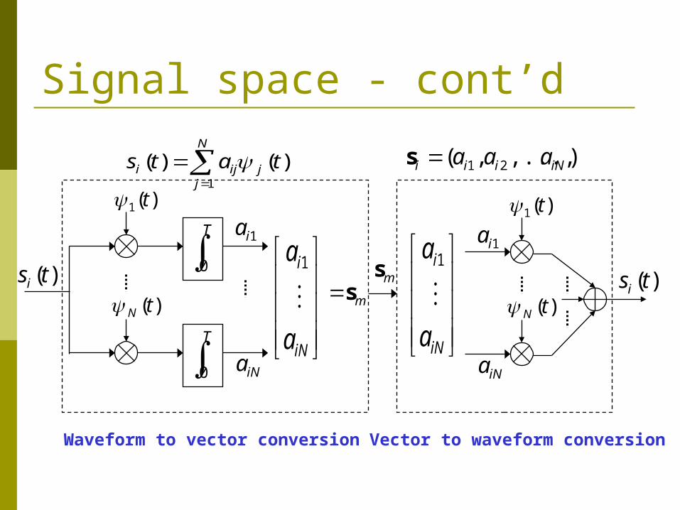
Signal space - cont’d
N
jjiji tats
1
)()( ),...,,( 21 iNiii aaas
iN
i
a
a
1
)(1 t
)(tN
1ia
iNa
)(tsi
T
0
)(1 t
T
0
)(tN
iN
i
a
a
1
ms)(tsi
1ia
iNa
ms
Waveform to vector conversion Vector to waveform conversion
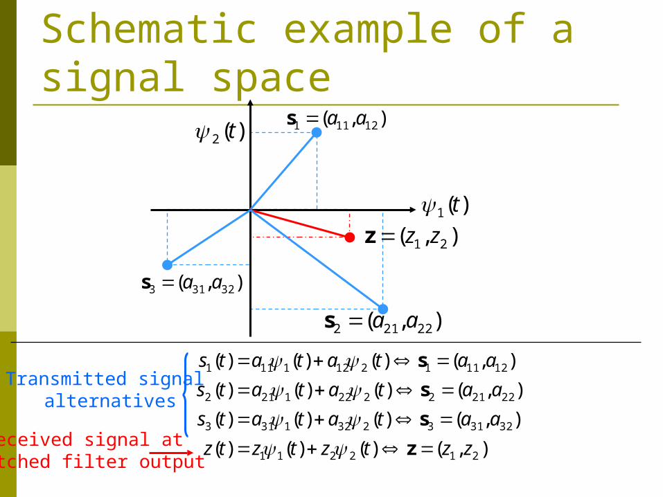
Schematic example of a signal space
),()()()(
),()()()(
),()()()(
),()()()(
212211
323132321313
222122221212
121112121111
zztztztz
aatatats
aatatats
aatatats
z
s
s
s
)(1 t
)(2 t ),( 12111 aas
),( 22212 aas
),( 32313 aas
),( 21 zzz
Transmitted signal alternatives
Received signal at matched filter output
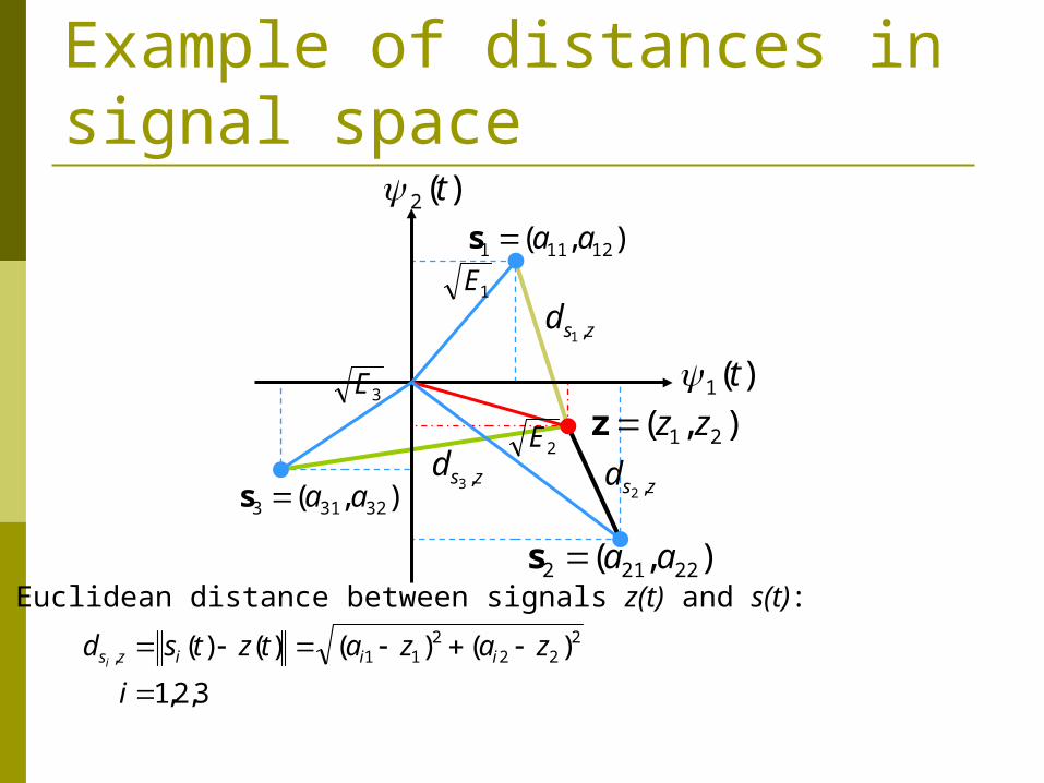
Example of distances in signal space
)(1 t
)(2 t),( 12111 aas
),( 22212 aas
),( 32313 aas
),( 21 zzz
zsd ,1
zsd ,2zsd ,3
The Euclidean distance between signals z(t) and s(t):
3,2,1
)()()()( 222
211,
i
zazatztsd iiizsi
1E
3E
2E
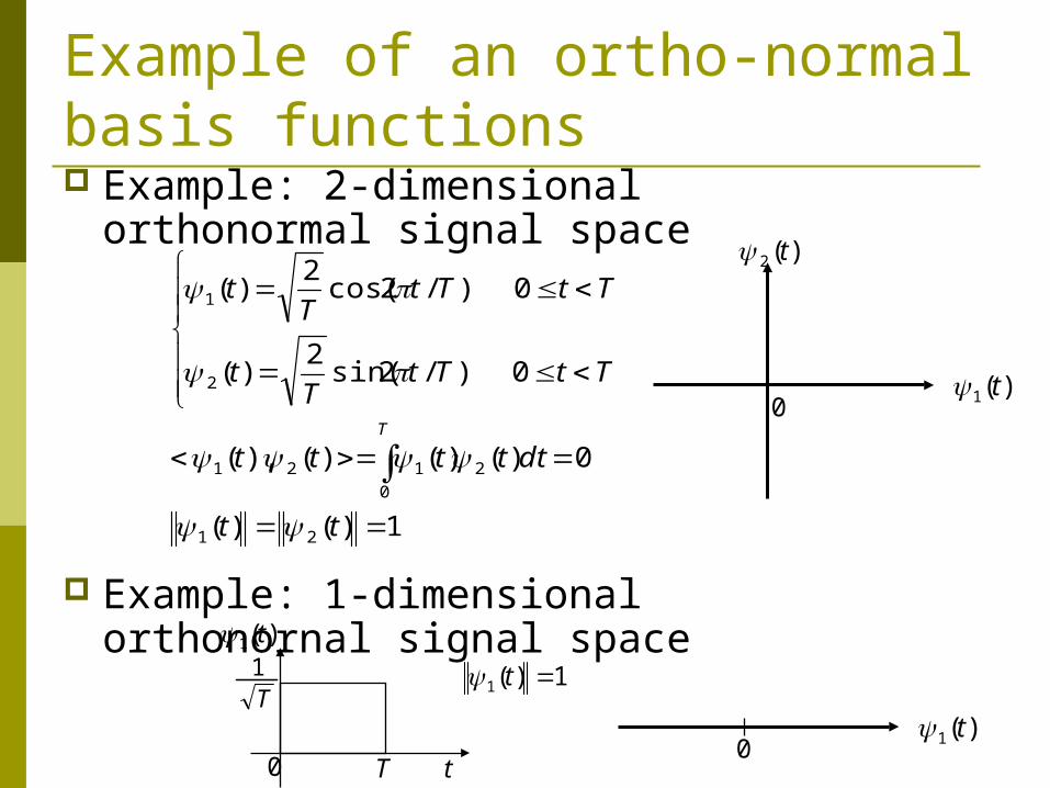
Example of an ortho-normal basis functions Example: 2-dimensional
orthonormal signal space
Example: 1-dimensional orthonornal signal space
1)()(
0)()()(),(
0)/2sin(2
)(
0)/2cos(2
)(
21
2
0
121
2
1
tt
dttttt
TtTtT
t
TtTtT
t
T
)(1 t
)(2 t
0
T t
)(1 t
T1
0
1)(1 t
)(1 t0
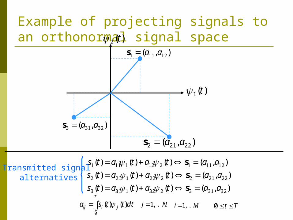
Example of projecting signals to an orthonormal signal space
),()()()(
),()()()(
),()()()(
323132321313
222122221212
121112121111
aatatats
aatatats
aatatats
s
s
s
)(1 t
)(2 t),( 12111 aas
),( 22212 aas
),( 32313 aas
Transmitted signal alternatives
dtttsaT
jiij )()(0 Tt 0Mi ,...,1Nj ,...,1
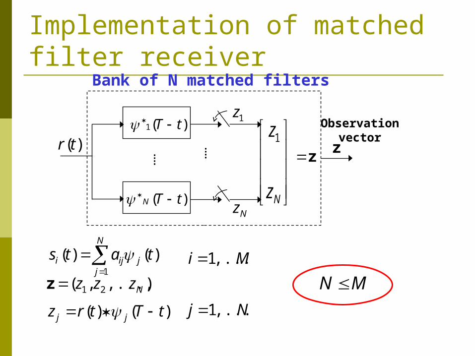
Implementation of matched filter receiver
)(tr
1z)(1 tT
)( tTN Nz
Bank of N matched filters
Observationvector
)()( tTtrz jj Nj ,...,1
),...,,( 21 Nzzzz
N
jjiji tats
1
)()(
MN Mi ,...,1
Nz
z1
z z

Implementation of correlator receiver
),...,,( 21 Nzzzz
Nj ,...,1dtttrz j
T
j )()(0
T
0
)(1 t
T
0
)(tN
Nr
r
1
z)(tr
1z
Nz
z
Bank of N correlators
Observationvector
N
jjiji tats
1
)()( Mi ,...,1
MN
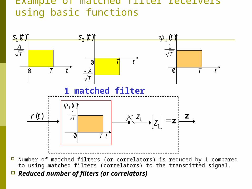
Example of matched filter receivers using basic functions
Number of matched filters (or correlators) is reduced by 1 compared to using matched filters (correlators) to the transmitted signal.
Reduced number of filters (or correlators)
T t
)(1 ts
T t
)(2 ts
T t
)(1 t
T1
0
1z z)(tr z
1 matched filter
T t
)(1 t
T1
0
1z
TA
TA0
0

26
Example 1.
27
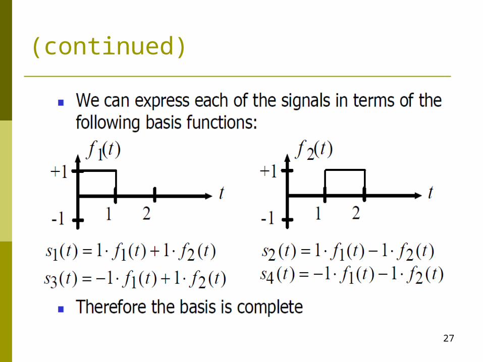
(continued)

28
(continued)

29
Signal Constellation for Ex.1
30
Notes on Signal Space Two entirely different signal sets can have the same geometric
representation. The underlying geometry will determine the performance and the
receiver structure for a signal set. In both of these cases we were fortunate enough to guess the correct
basis functions. Is there a general method to find a complete orthonormal basis for an
arbitrary signal set? Gram-Schmidt Procedure
31
Gram-Schmidt Procedure
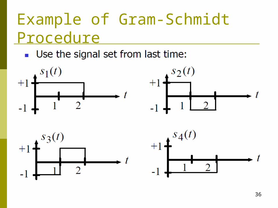
Suppose we are given a signal set:
We would like to find a complete orthonormal basis for this signal set.
The Gram-Schmidt procedure is an iterative procedure for creating an orthonormal basis.
1{ ( ),..........., ( )}Ms t s t
1{ ( ),.........., ( )}, Kf t f t K M
32
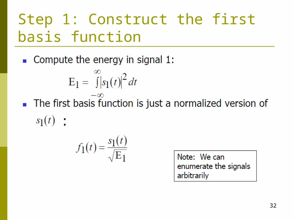
Step 1: Construct the first basis function
33
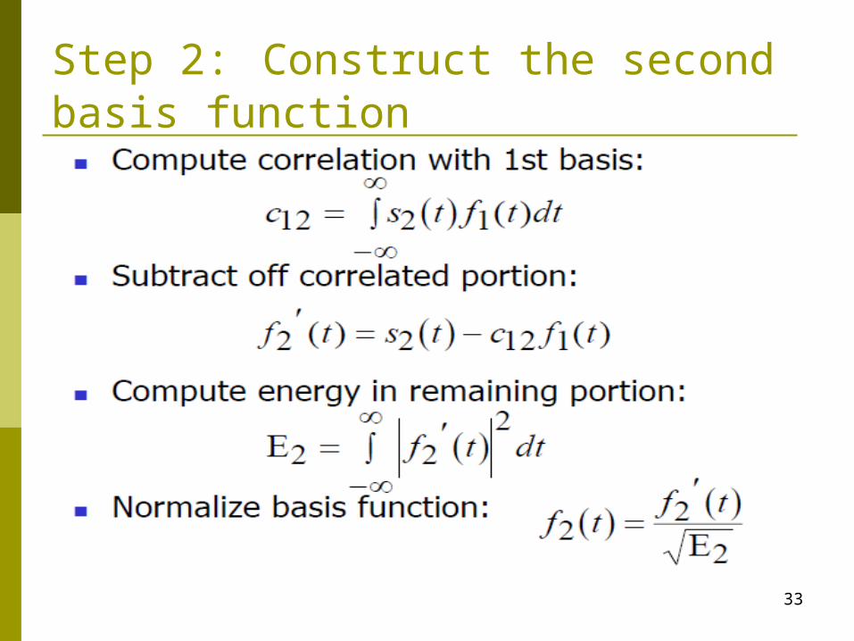
Step 2: Construct the second basis function

34
Procedure for the successive signals

35
Summary of Gram-Schmidt Prodcedure
36
Example of Gram-Schmidt Procedure

37
Step 1:
38
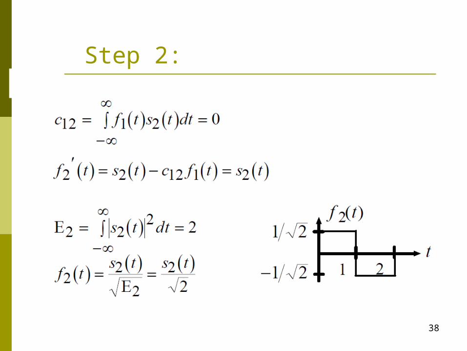
Step 2:
39
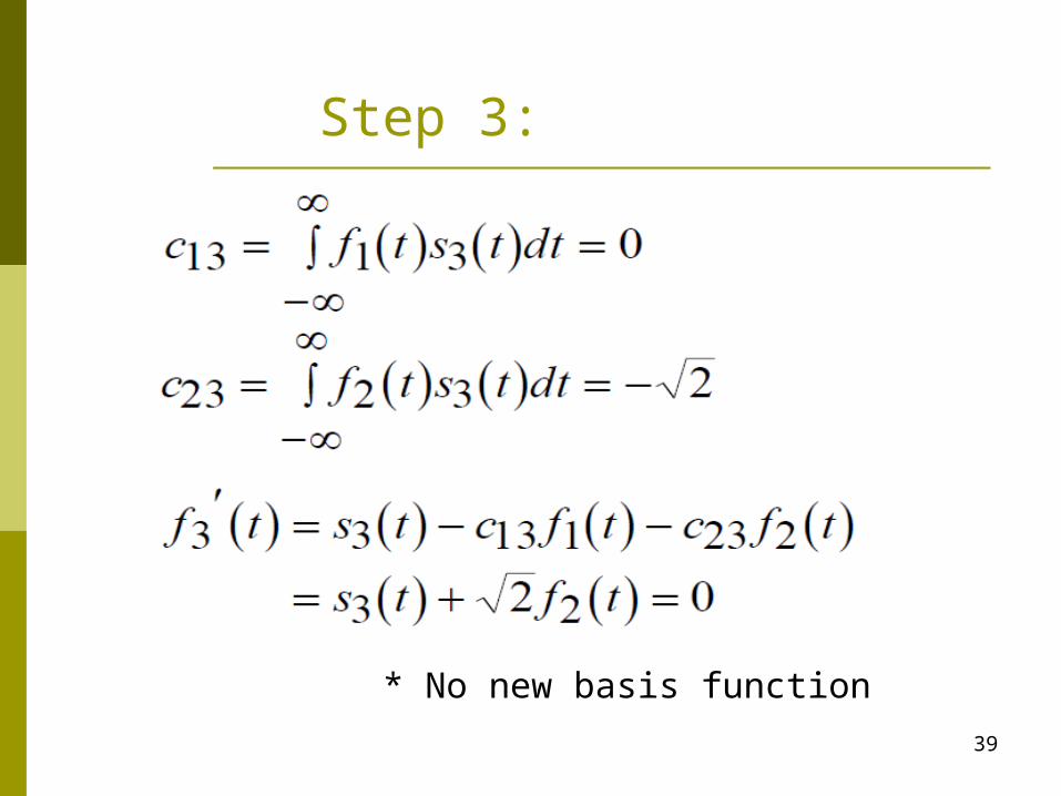
Step 3:
* No new basis function

40
Step 4:
* No new basis function. Procedure is complete
41
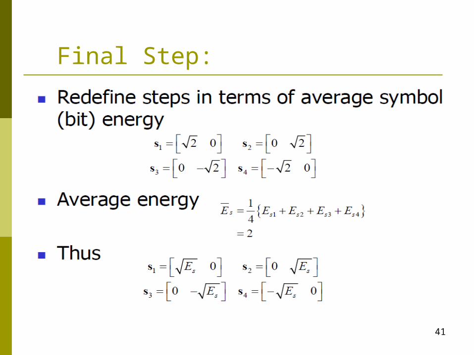
Final Step:

42
Signal Constellation Diagram

Bandpass Signals
Representation
44
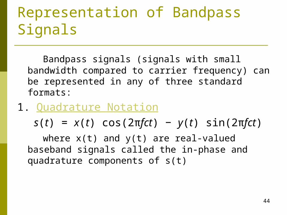
Representation of Bandpass Signals
Bandpass signals (signals with small bandwidth compared to carrier frequency) can be represented in any of three standard formats:
1. Quadrature Notation s(t) = x(t) cos(2πfct) − y(t) sin(2πfct) where x(t) and y(t) are real-valued baseband signals called the in-
phase and quadrature components of s(t)
45
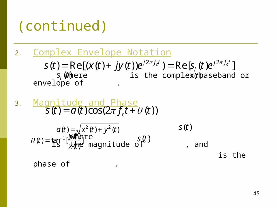
(continued)
2. Complex Envelope Notation
where is the complex baseband or envelope of . 3. Magnitude and Phase
where is the magnitude of , and is the phase of .
2 2( ) Re[( ( ) ( )) ) Re[ ( ) ]c cj f t j f tls t x t jy t e s t e
( )ls t ( )s t
( ) ( )cos(2 ( ))cs t a t f t t 2 2( ) ( ) ( )a t x t y t ( )s t
1 ( )( ) tan [ ]
( )
y tt
x t ( )s t
46
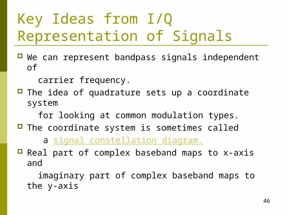
Key Ideas from I/QRepresentation of Signals We can represent bandpass signals independent of carrier frequency. The idea of quadrature sets up a coordinate system for looking at common modulation types. The coordinate system is sometimes called a signal constellation diagram. Real part of complex baseband maps to x-axis and imaginary part of complex baseband maps to the y-axis

47
Constellation Diagrams
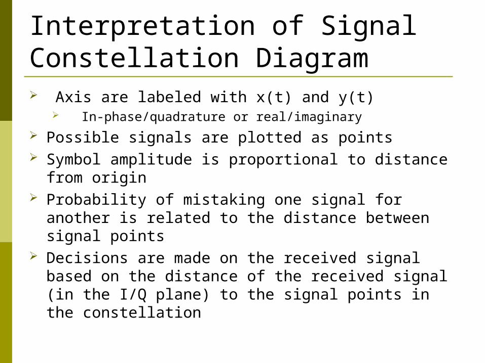
Interpretation of Signal Constellation Diagram Axis are labeled with x(t) and y(t)
In-phase/quadrature or real/imaginary Possible signals are plotted as points Symbol amplitude is proportional to distance from
origin Probability of mistaking one signal for another is
related to the distance between signal points Decisions are made on the received signal based
on the distance of the received signal (in the I/Q plane) to the signal points in the constellation
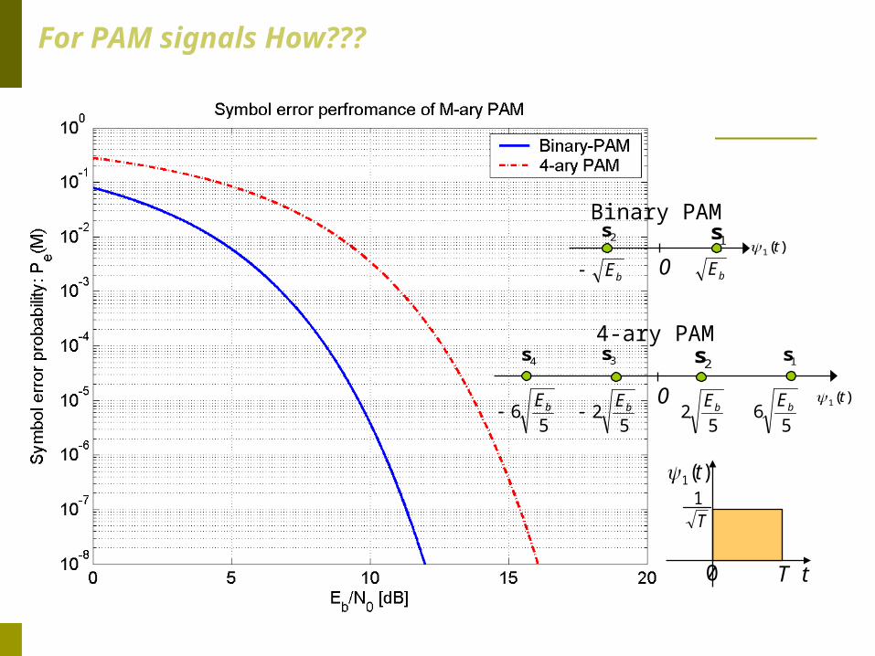
For PAM signals How???
)(1 t0
1s2s
bEbE
Binary PAM
)(1 t0
2s3s
52 bE
56 bE
56 bE
5
2 bE
4s 1s4-ary PAM
T t
)(1 t
T1
0