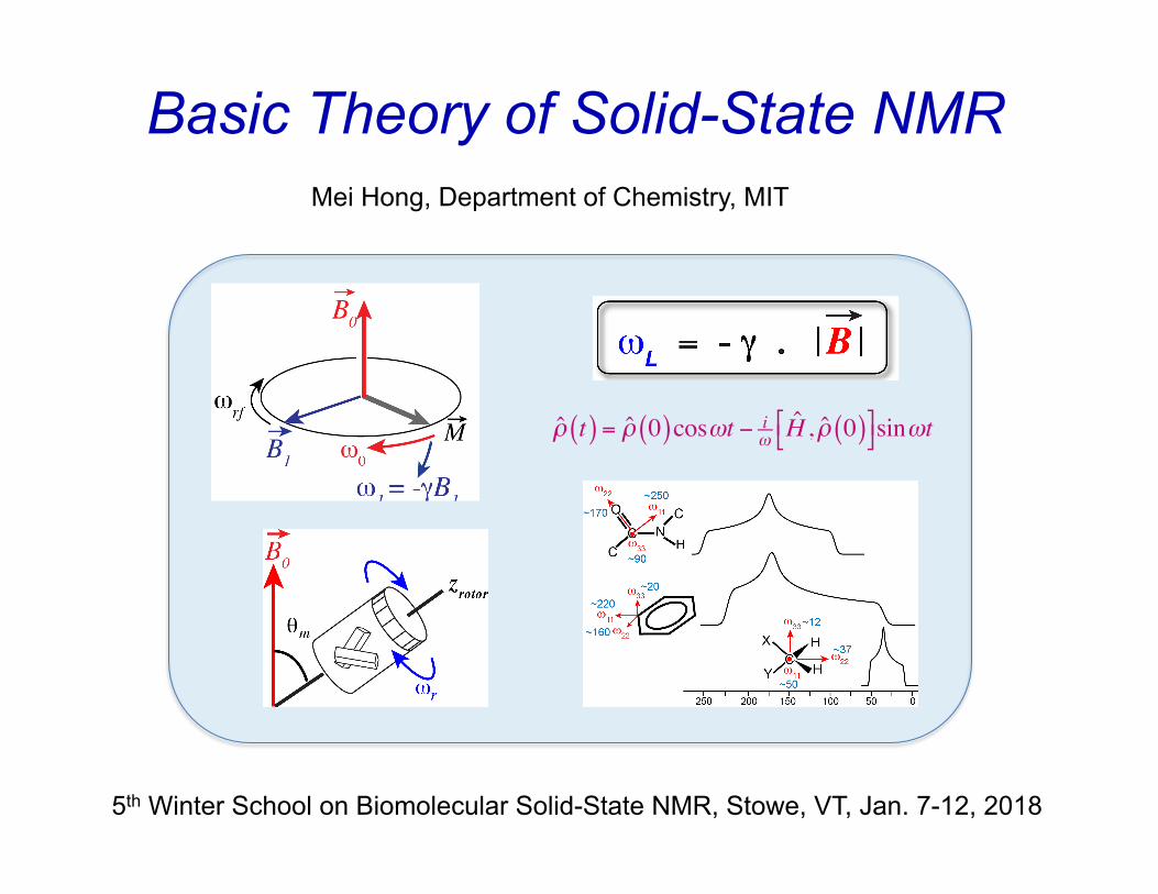
Basic Theory of Solid-State NMR

ρ t( ) = ρ 0( )cosωt − iω H , ρ 0( )$%

&'sinωt

5th Winter School on Biomolecular Solid-State NMR, Stowe, VT, Jan. 7-12, 2018

Mei Hong, Department of Chemistry, MIT

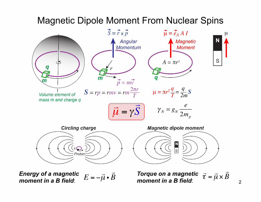
Magnetic Dipole Moment From Nuclear Spins

2

µ = γ

S γ N = gN

e2mp

E = −µ iB

τ =µ ×BEnergy of a magnetic

moment in a B field: Torque on a magnetic moment in a B field:

τ =µ ×B

τ =

dSdt

=1γd µdt

$

%&

'&⇒ dµdt

= γµ ×B

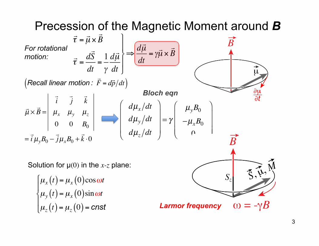
Precession of the Magnetic Moment around B

3

For rotational motion:

Recall linear motion : F = dp dt( )

Solution for µ(0) in the x-z plane:

µx t( ) = µx 0( )cosωtµy t( ) = µx 0( )sinωtµz t( ) = µz 0( ) = cnst

"

#$

%$

!µ ×!B =

i!

j!

k!

µx µy µz0 0 B0

=!i µyB0 −

!jµxB0 +

!k ⋅0

Bloch eqn

dµx dtdµy dt

dµz dt

⎛

⎝

⎜⎜⎜

⎞

⎠

⎟⎟⎟= γ

µyB0−µxB00

⎛

⎝

⎜⎜⎜

⎞

⎠

⎟⎟⎟

Larmor frequency

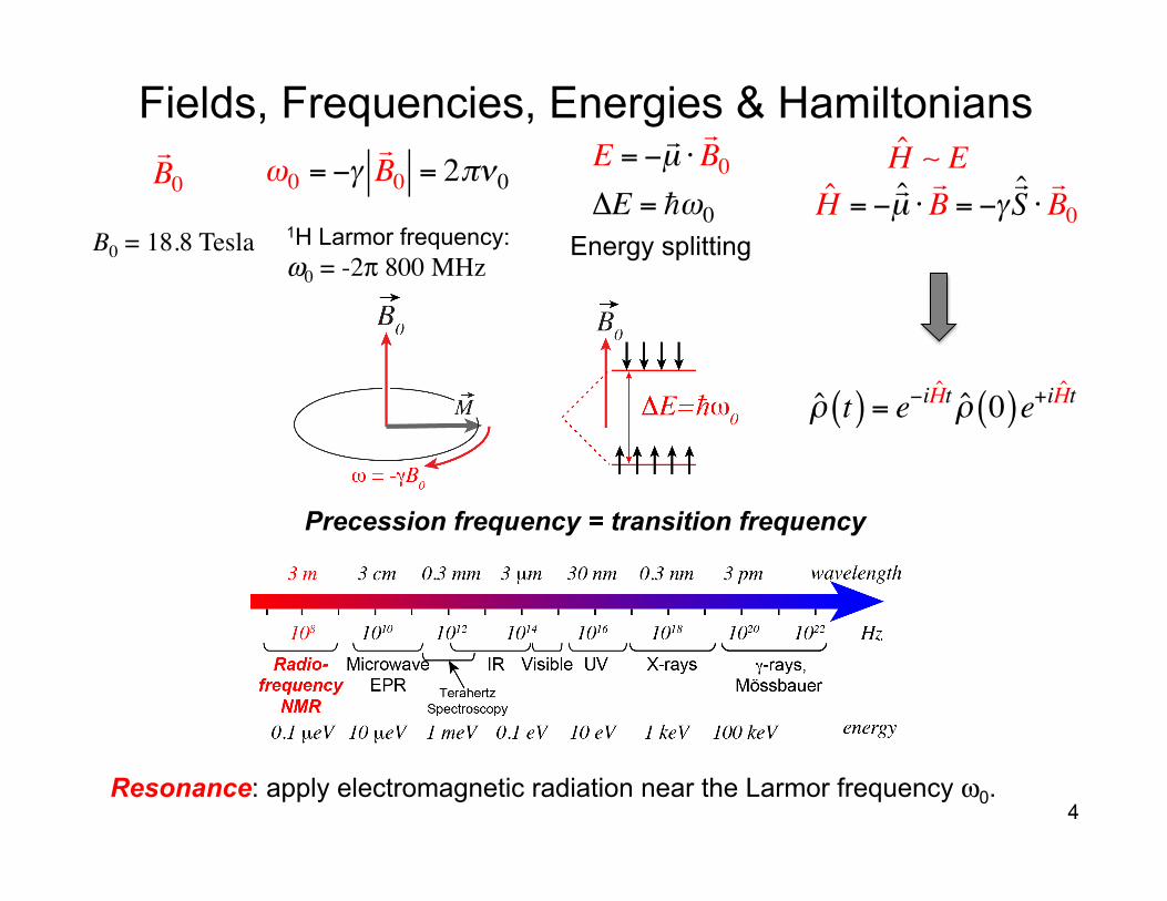
Fields, Frequencies, Energies & Hamiltonians

Precession frequency = transition frequency

ρ t( ) = e−iHt ρ 0( )e+iHt

4

H EH = −

µ ⋅B = −γ

S ⋅B0

E = − µ ⋅B0

ΔE = ω0 B0

B0 = 18.8 Tesla 1H Larmor frequency: ω0 = -2π 800 MHz

Energy splitting

ω0 = −γB0 = 2πν0

Resonance: apply electromagnetic radiation near the Larmor frequency ω0.

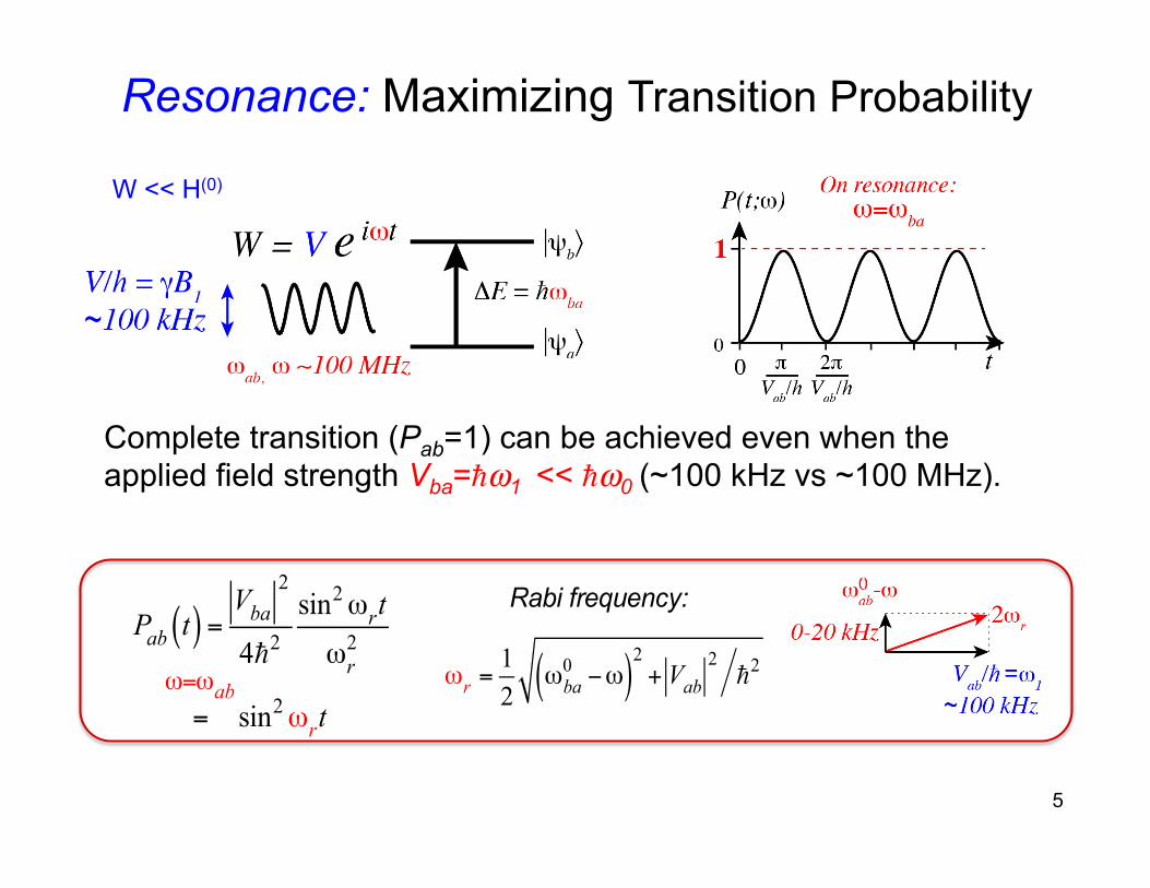
Resonance: Maximizing Transition Probability

Complete transition (Pab=1) can be achieved even when the applied field strength Vba=ħω1 << ħω0  (~100 kHz vs ~100 MHz).

W << H(0)

5

Pab t( ) =Vba

2

42

sin2ωrtωr

2

=ω=ωab

sin2ωrt

Rabi frequency:

ωr =12

ωba0 −ω( )

2+ Vab

22

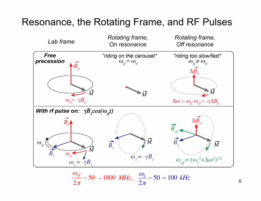
Resonance, the Rotating Frame, and RF Pulses

Lab frame Rotating frame, On resonance

Rotating frame, Off resonance

6 ωrf

2π 50 –1000 MHz, ω1

2π 50 – 100 kHz

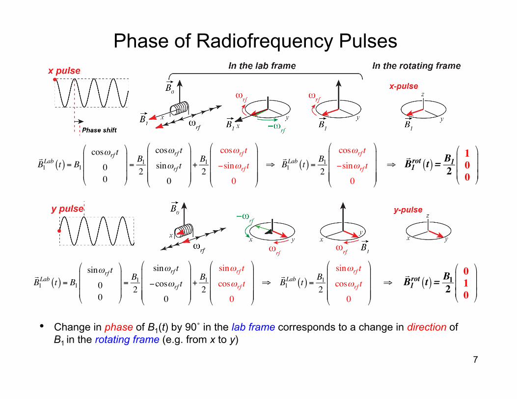
Phase of Radiofrequency Pulses

•  Change in phase of B1(t) by 90˚ in the lab frame corresponds to a change in direction of B1 in the rotating frame (e.g. from x to y)

B1Lab t( ) = B1

cosωrf t

00

"

#

$$$

%

&

'''=B12

cosωrf t

sinωrf t

0

"

#

$$$$

%

&

''''+B12

cosωrf t

−sinωrf t

0

"

#

$$$$

%

&

'''' ⇒

B1Lab t( ) = B1

2

cosωrf t

−sinωrf t

0

"

#

$$$$

%

&

'''' ⇒

B1rot t( ) =

B12

100

"

#

$$$

%

&

'''

7

B1Lab t( ) = B1

sinωrf t

00

"

#

$$$

%

&

'''=B12

sinωrf t

−cosωrf t

0

"

#

$$$$

%

&

''''+B12

sinωrf t

cosωrf t

0

"

#

$$$$

%

&

'''' ⇒

B1Lab t( ) = B1

2

sinωrf t

cosωrf t

0

"

#

$$$$

%

&

'''' ⇒

B1rot t( ) =

B12

010

"

#

$$$

%

&

'''

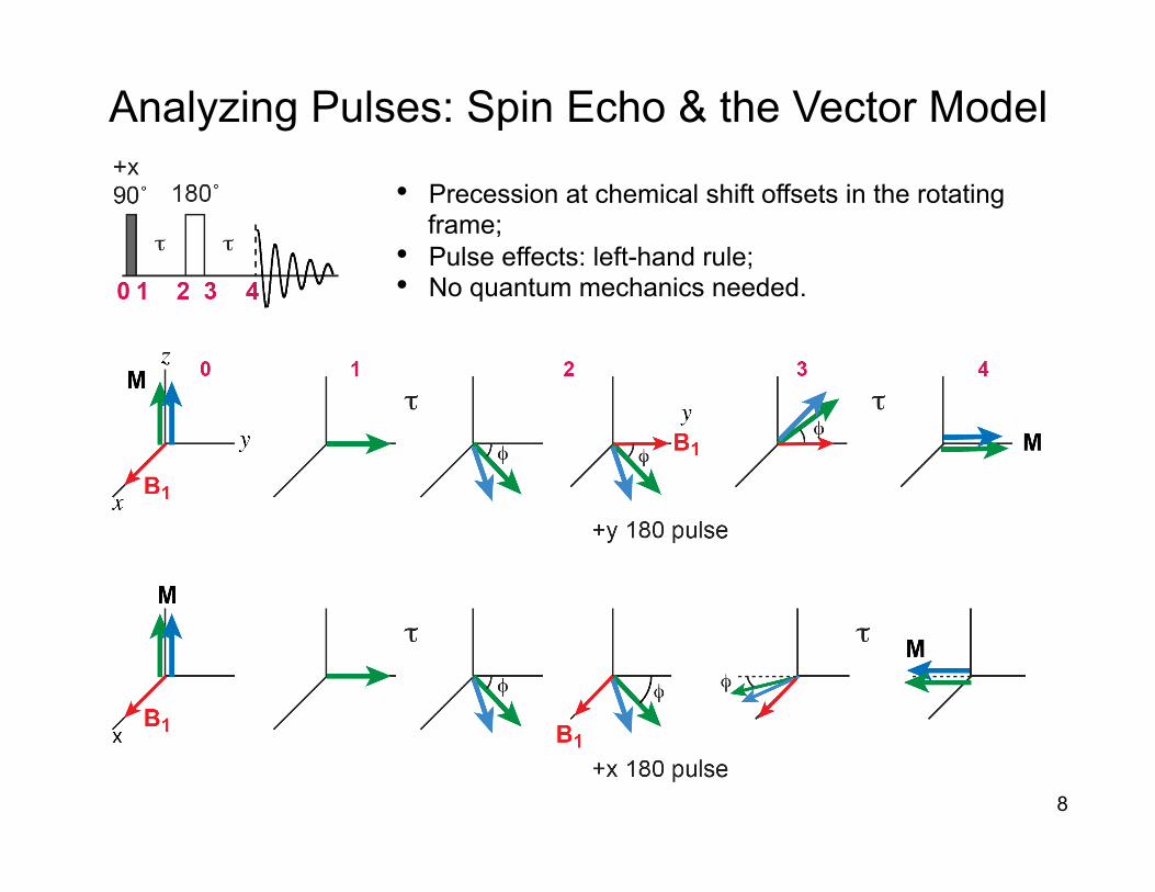
Analyzing Pulses: Spin Echo & the Vector Model

•  Precession at chemical shift offsets in the rotating frame;

•  Pulse effects: left-hand rule; •  No quantum mechanics needed.

8

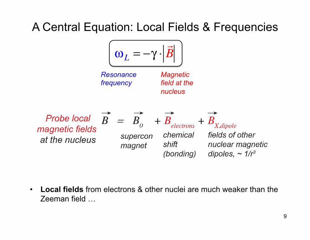
A Central Equation: Local Fields & Frequencies

9

•  Local fields from electrons & other nuclei are much weaker than the Zeeman field …

ωL = −γ ⋅!B

Resonance frequency

Magnetic field at the nucleus

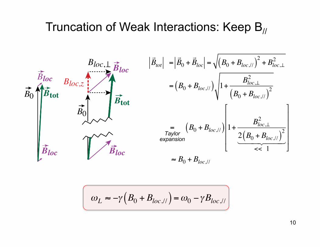
Truncation of Weak Interactions: Keep B//

Btot =

B0 +

Bloc = B0 + Bloc,//( )2 + Bloc,⊥2

= B0 + Bloc,//( ) 1+Bloc,⊥2

B0 + Bloc,//( )2

= Taylor expansion

B0 + Bloc,//( ) 1+Bloc,⊥2

2 B0 + Bloc,//( )2

<< 1

"

#

$$$$

%

&

''''

≈ B0 + Bloc,//

ωL ≈ −γ B0 + Bloc,//( ) =ω0 −γBloc,//

10

HZeeman = −γ I zB0

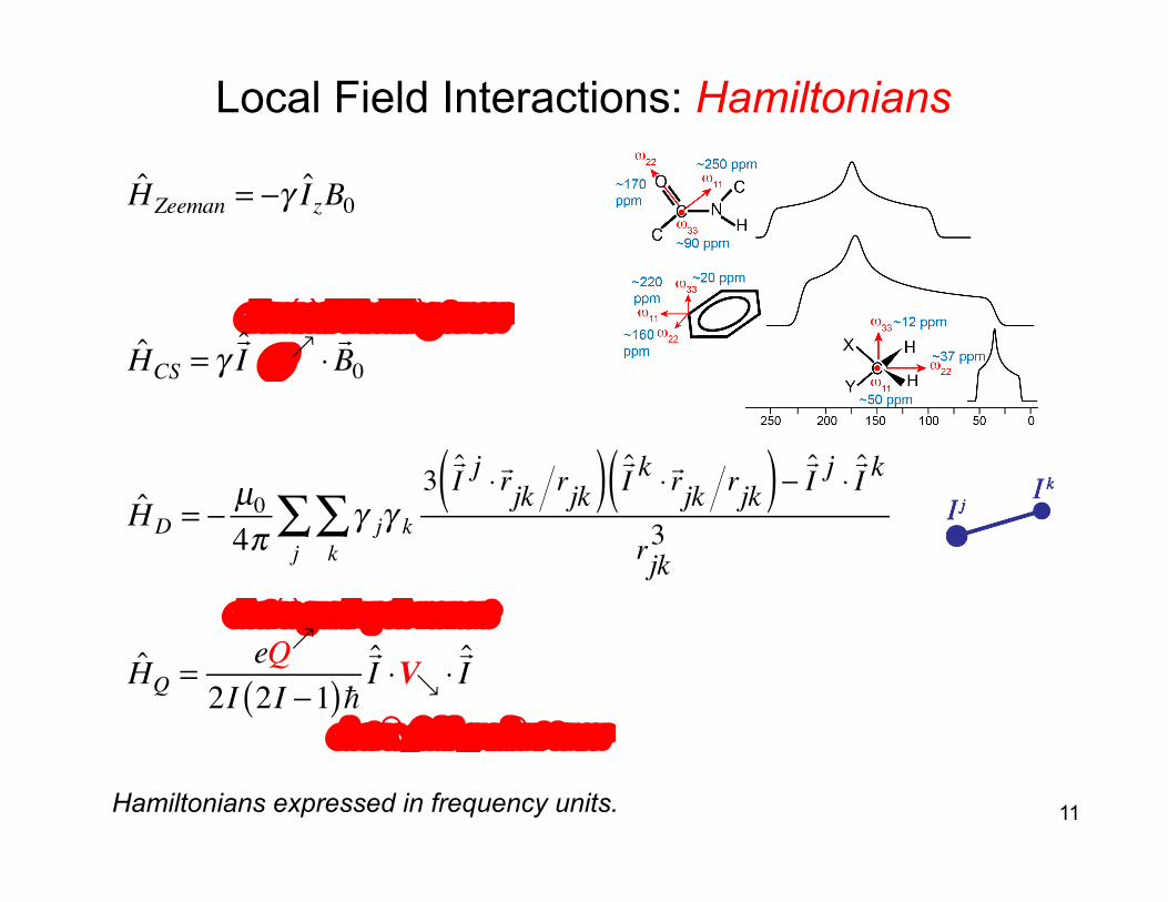
11 Hamiltonians expressed in frequency units.

chemical shielding tensor

HCS = γ!I ⋅σ↗ ⋅

!B0

HD = − µ04π

γ jγ k3!I j ⋅ !rjk rjk( ) !I k ⋅ !rjk rjk( )− !I j ⋅ !I k

rjk3

k∑

j∑

electric quadrupole moment

HQ = e ↗Q2I 2I −1( )"

#I ⋅V↘ ⋅

#I

electric field gradient tensor

Local Field Interactions: Hamiltonians

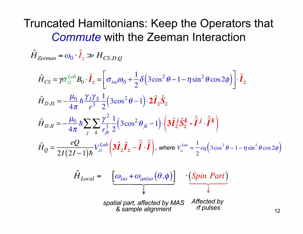
HCS = γσ zzLabB0 ⋅ Iz = σ isoω0 +

12δ 3cos2θ −1−η sin2θ cos2φ( )⎡

⎣⎢⎤⎦⎥⋅ Iz

HD,IS = − µ04π!γ Iγ Sr3

123cos2θ −1( ) ⋅2 IzSz

HD,II = − µ04π!

γ 2

rjk3123cos2θ jk −1( )

k∑

j∑ ⋅ 3Izj Szk -

"I j ⋅"I k( )

HQ = eQ2I 2I −1( )!Vzz

Lab 3Iz Iz −"I ⋅"I( ), where Vzz

Lab =1

2eq 3cos2 θ − 1− η sin2 θ cos 2φ( )

Truncated Hamiltonians: Keep the Operators that Commute with the Zeeman Interaction

HLocal = ωiso +ωaniso θ ,φ( )$% &'

↓

spatial part, affected by MAS& sample alignment

⋅ Spin Part( )

↓

Affected by rf pulses

12

HZeeman =ω0 ⋅ I z HCS,D,Q

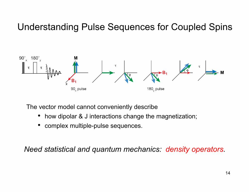
Understanding Pulse Sequences for Coupled Spins

The vector model cannot conveniently describe •  how dipolar & J interactions change the magnetization; •  complex multiple-pulse sequences.

14

Need statistical and quantum mechanics: density operators.

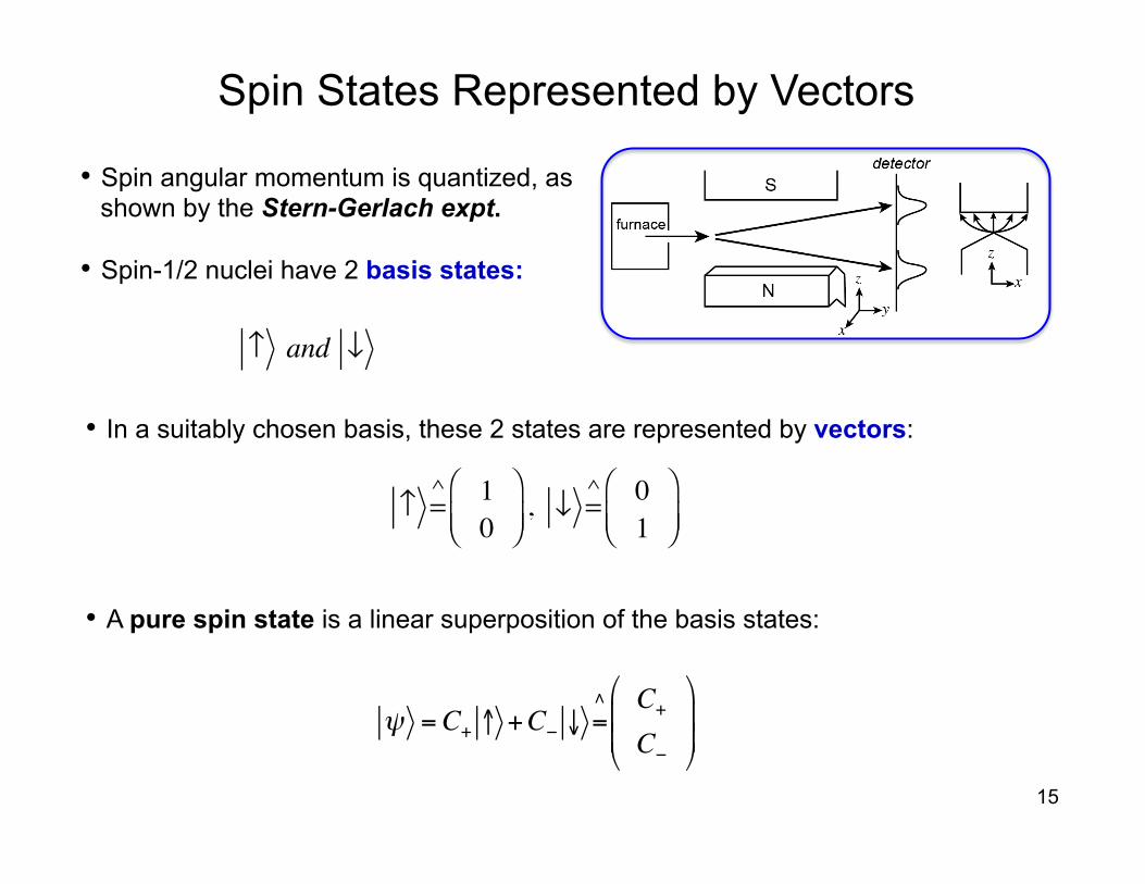
•  Spin angular momentum is quantized, as shown by the Stern-Gerlach expt.

•  Spin-1/2 nuclei have 2 basis states:

Spin States Represented by Vectors

↑ =

∧ 10

⎛⎝⎜

⎞⎠⎟, ↓ =

∧ 01

⎛⎝⎜

⎞⎠⎟

↑ and ↓

ψ =C+ ↑ +C− ↓ =∧ C+

C−

&

'((

)

*++

15

•  In a suitably chosen basis, these 2 states are represented by vectors:

•  A pure spin state is a linear superposition of the basis states:

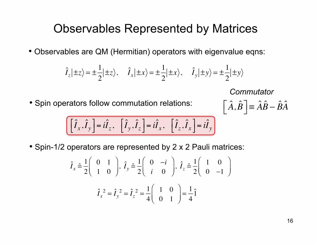
• Observables are QM (Hermitian) operators with eigenvalue eqns:

A, B⎡⎣ ⎤⎦ ≡ AB − BA

I x , I y!"

#$= iIz , I y , I z!

"#$= iI x , I z , I x!

"#$= iI y

Observables Represented by Matrices

•  Spin operators follow commutation relations:

•  Spin-1/2 operators are represented by 2 x 2 Pauli matrices:

I z ±z = ± 1

2±z , I x ±x = ± 1

2±x , I y ±y = ± 1

2±y

I x =

12

0 11 0

⎛⎝⎜

⎞⎠⎟, I y =

12

0 −ii 0

⎛⎝⎜

⎞⎠⎟, I z =

12

1 00 −1

⎛⎝⎜

⎞⎠⎟

I x2 = I y

2 = I z2 = 1

41 00 1

⎛⎝⎜

⎞⎠⎟= 141

16

Commutator

Our Samples: an Ensemble of Spins •  Expectation (average) value of an observable A:

•  The observable in NMR is the magnetization...

•  At thermal equilibrium:

ρeq =e−H kT

Tr e−H kT( )≈

12I +1

1− HkT

$

%&

'

()

Dropped: commutes with all operators

Trace, sum of diagonal ω0 << kT

ρeq' ≈

12I +1

γB0kT

Iz$

%&

'

() ∝ I z

17

For pure states: = C+* C−

*( ) A++ A+−A−+ A−−

⎛

⎝⎜

⎞

⎠⎟

C+

C−

⎛

⎝⎜

⎞

⎠⎟ =

C+*C+A++ + C−

*C−A−−

+C+*C−A+− + C−

*C+A−+

A ≡ ψ Aψ

ρ ≡ pk ψ k ψ kk∑ = pk

Ck+

Ck−

⎛

⎝⎜

⎞

⎠⎟ Ck+

* Ck−*( )

k

∑ =C+C+

* C+C−*

C−C+* C−C−

*

⎛

⎝

⎜⎜

⎞

⎠

⎟⎟

•  A statistical ensemble of spins is described by a density operator:

For mixtures: A = pk ψ k Aψ k = ∑ Tr ρ A( )

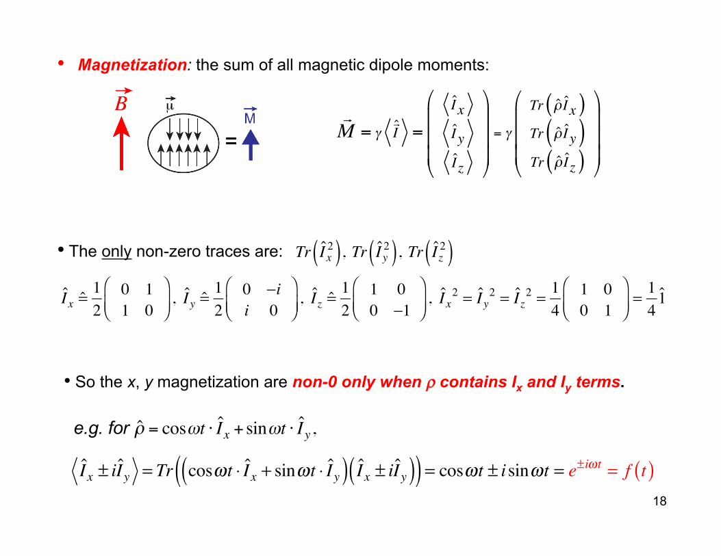
•  Magnetization: the sum of all magnetic dipole moments:

M = γ

I =

I x

I y

I z

"

#

$$$

%

&

'''= γ

Tr ρ I x( )Tr ρ I y( )Tr ρ I z( )

"

#

$$$

%

&

'''

18

I x =

12

0 11 0

⎛⎝⎜

⎞⎠⎟, I y =

12

0 −ii 0

⎛⎝⎜

⎞⎠⎟, I z =

12

1 00 −1

⎛⎝⎜

⎞⎠⎟, I x

2 = I y2 = I z

2 = 14

1 00 1

⎛⎝⎜

⎞⎠⎟= 141

Tr Ix

2( ), Tr Iy2( ), Tr Iz

2( )•  The only non-zero traces are:

I x ± iI y = Tr cosωt ⋅ I x + sinωt ⋅ I y( ) I x ± iI y( )( ) = cosωt ± isinωt = e±iωt = f t( ) e.g. for ρ = cosωt ⋅ I x + sinωt ⋅ I y ,

•  So the x, y magnetization are non-0 only when ρ contains Ix and Iy terms.

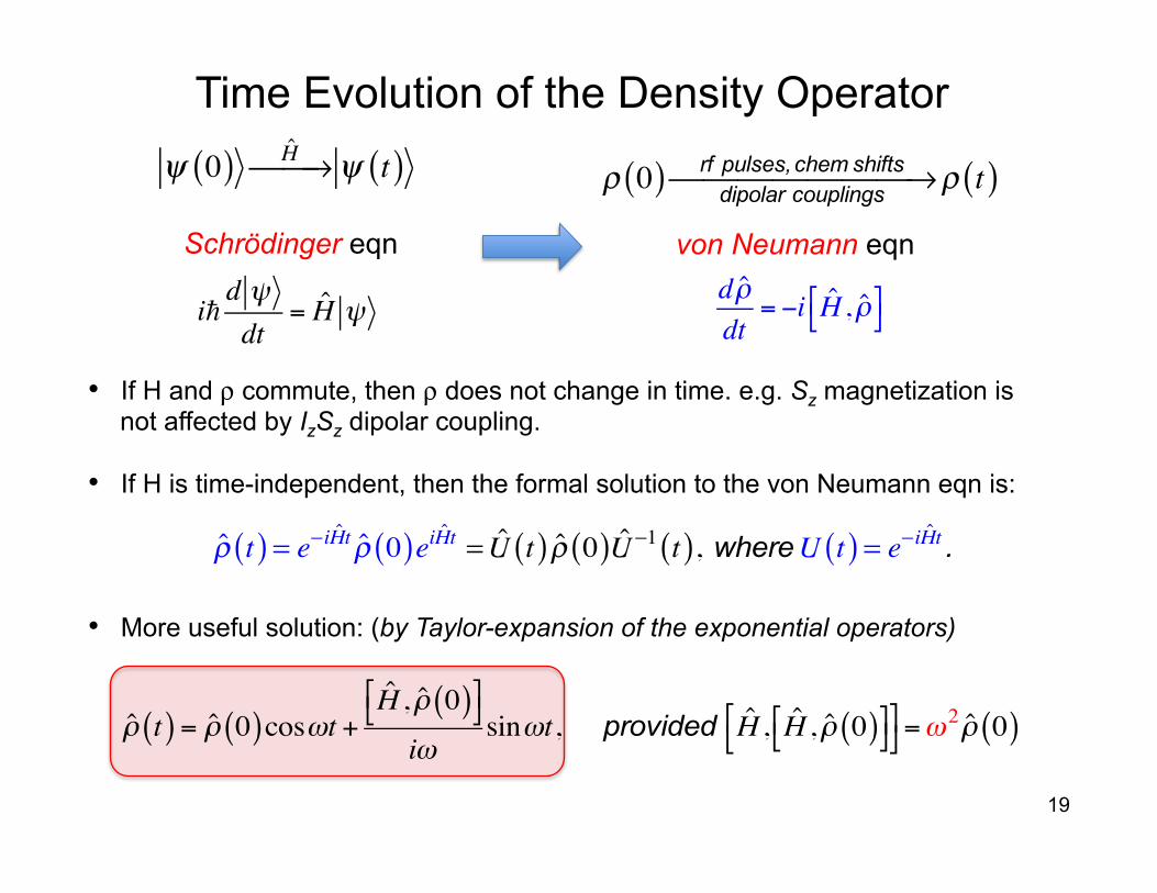
Time Evolution of the Density Operator

19

•  If H and ρ commute, then ρ does not change in time. e.g. Sz magnetization is not affected by IzSz dipolar coupling.

id ψdt

= H ψ

ψ 0( ) H⎯ →⎯ ψ t( )

Schrödinger eqn  dρdt

= −i H , ρ#$

%&

von Neumann eqn   ρ 0( ) rf pulses, chem shifts

dipolar couplings⎯ →⎯⎯⎯⎯⎯⎯ ρ t( )

ρ t( ) = e−iHt ρ 0( )eiHt = U t( ) ρ 0( )U−1 t( ), where U t( ) = e−iHt .

•  If H is time-independent, then the formal solution to the von Neumann eqn is:

ρ t( ) = ρ 0( )cosωt +

H , ρ 0( )#$

%&

iωsinωt, provided H , H , ρ 0( )#

$%&

#$

%&=ω

2ρ 0( )

•  More useful solution: (by Taylor-expansion of the exponential operators)

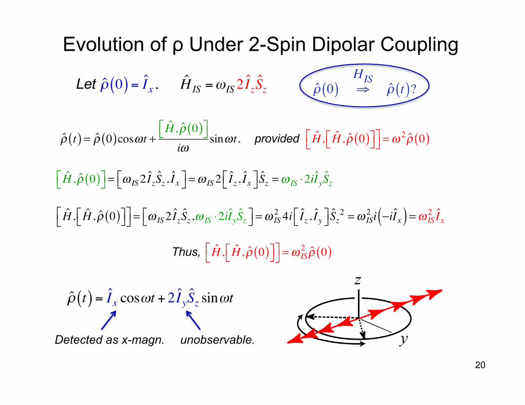
Evolution of ρ Under 2-Spin Dipolar Coupling

Let ρ 0( ) = I x , H IS =ωIS2 I zSz

ρ t( ) = ρ 0( )cosωt +

H , ρ 0( )⎡⎣ ⎤⎦iω

sinωt, provided H , H , ρ 0( )⎡⎣ ⎤⎦⎡⎣

⎤⎦ =ω

2ρ 0( )

Thus, H , H , ρ 0( )⎡⎣ ⎤⎦⎡

⎣⎤⎦ =ω IS

2 ρ 0( )

ρ 0( ) ⇒HIS

ρ t( )?

ρ t( ) = I x cosωt +2 I ySz sinωt

Detected as x-magn. unobservable.

20

H , ρ 0( )⎡⎣ ⎤⎦ = ω IS2 I zSz , I x⎡⎣ ⎤⎦ =ω IS2 I z , I x⎡⎣ ⎤⎦ Sz =ω IS ⋅2iI ySz

H , H , ρ 0( )⎡⎣ ⎤⎦⎡⎣

⎤⎦ = ω IS2 I zSz ,ω IS ⋅2iI ySz⎡⎣ ⎤⎦ =ω IS

2 4i Iz , I y⎡⎣ ⎤⎦ Sz2 =ω IS

2 i −iI x( ) =ω IS2 I x

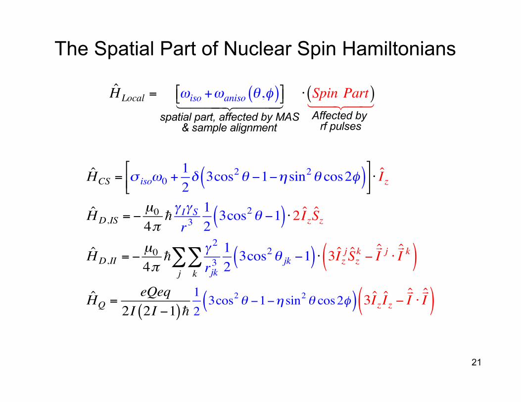
HCS = σ isoω0 +12δ 3cos2θ −1−η sin2θ cos2φ( )(

)*+

,-⋅ I z

HD,IS = −µ04πγ IγSr3

123cos2θ −1( ) ⋅2 I zSz

HD,II = −µ04π

γ 2

rjk3123cos2θ jk −1( )

k∑

j∑ ⋅ 3I z

jSzk −I j ⋅I k( )

HQ =eQeq

2I 2I −1( )123cos2θ −1−η sin2θ cos2φ( ) 3I z Iz −

I ⋅I( )

The Spatial Part of Nuclear Spin Hamiltonians

HLocal = ωiso +ωaniso θ ,φ( )$% &'spatial part, affected by MAS

& sample alignment

⋅ Spin Part( )

Affected by rf pulses

21

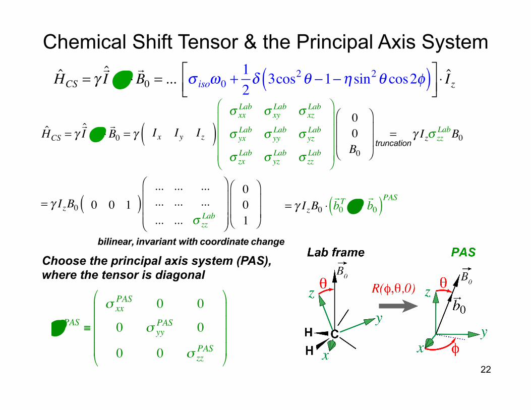
Chemical Shift Tensor & the Principal Axis System

HCS = γ

!I ⋅"σ ⋅!B0 = ... σ isoω0 +

12δ 3cos2θ −1−η sin2θ cos2φ( )⎡

⎣⎢⎤⎦⎥⋅ I z

HCS = γ!I ⋅"σ ⋅!B0 = γ Ix Iy Iz( )

σ xxLab σ xy

Lab σ xzLab

σ yxLab σ yy

Lab σ yzLab

σ zxLab σ yz

Lab σ zzLab

⎛

⎝

⎜⎜⎜⎜

⎞

⎠

⎟⎟⎟⎟

00B0

⎛

⎝

⎜⎜

⎞

⎠

⎟⎟

=truncation

γ Izσ zzLabB0

= γ IzB0 0 0 1( )... ... ...... ... ...... ... σ zz

Lab

⎛

⎝

⎜⎜⎜

⎞

⎠

⎟⎟⎟

001

⎛

⎝

⎜⎜

⎞

⎠

⎟⎟

Choose the principal axis system (PAS), where the tensor is diagonal

σ PAS ≡

σ xxPAS 0 0

0 σ yyPAS 0

0 0 σ zzPAS

#

$

%%%%

&

'

((((

22

= γ IzB0 ⋅

!b0T "σ !b0( )PAS

bilinear, invariant with coordinate change

= cosφ sinθ , sinφ sinθ , cosθ( )

ωxxPAS 0 0

0 ωyyPAS 0

0 0 ωzzPAS

$

%

&&&&

'

(

))))

cosφ sinθsinφ sinθcosθ

$

%

&&&

'

(

)))

b0PAS

Iz

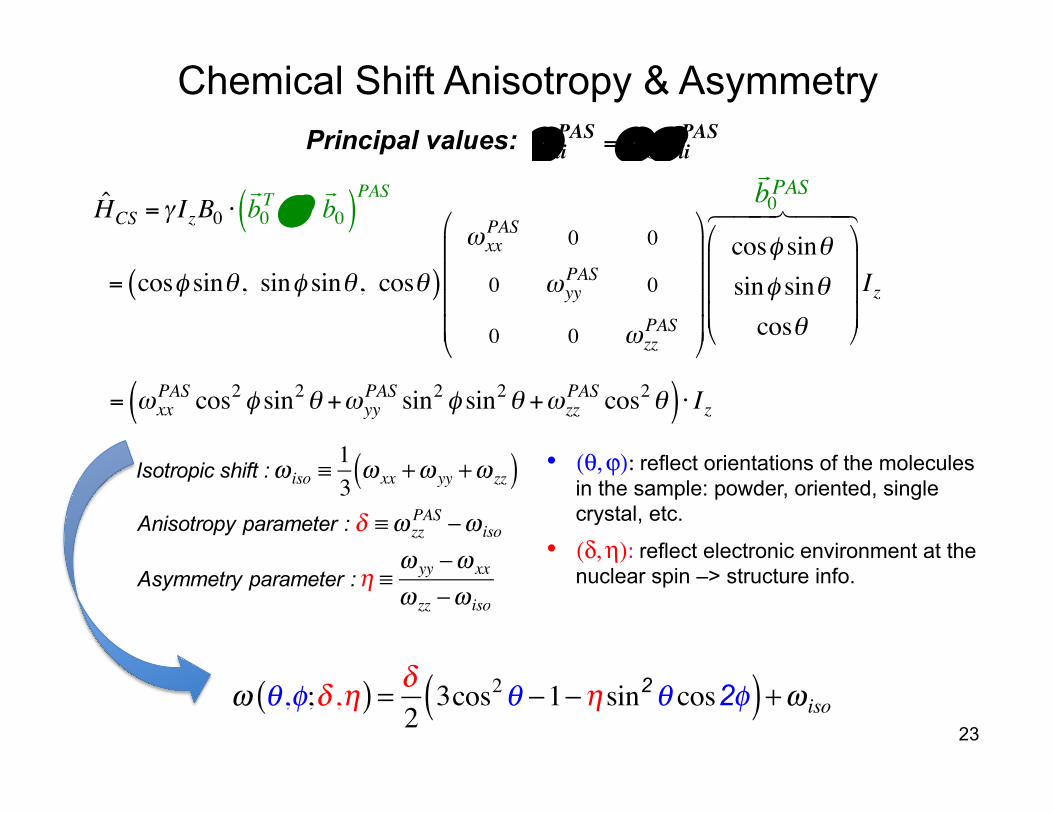
Chemical Shift Anisotropy & Asymmetry Principal values: ω ii

PAS =ω0σ iiPAS

= ωxxPAS cos2 φ sin2θ +ωyy

PAS sin2 φ sin2θ +ωzzPAS cos2θ( ) ⋅ Iz

HCS = γ IzB0 ⋅

b0T σ b0( )

PAS

Isotropic shift : ω iso ≡13ω xx +ω yy +ω zz( )

Anisotropy parameter : δ ≡ω zzPAS −ω iso

Asymmetry parameter : η ≡ω yy −ω xx

ω zz −ω iso

Directional cosines

Chemical shift anisotropy can also be expressed in terms of directional cosines.

•  (θ, ϕ):  reflect orientations of the molecules in the sample: powder, oriented, single crystal, etc.  

•  (δ, η):  reflect electronic environment at the nuclear spin –> structure info.

23 ω θ ,φ;δ ,η( ) = δ

23cos2θ −1−η sin2θ cos2φ( ) +ω iso

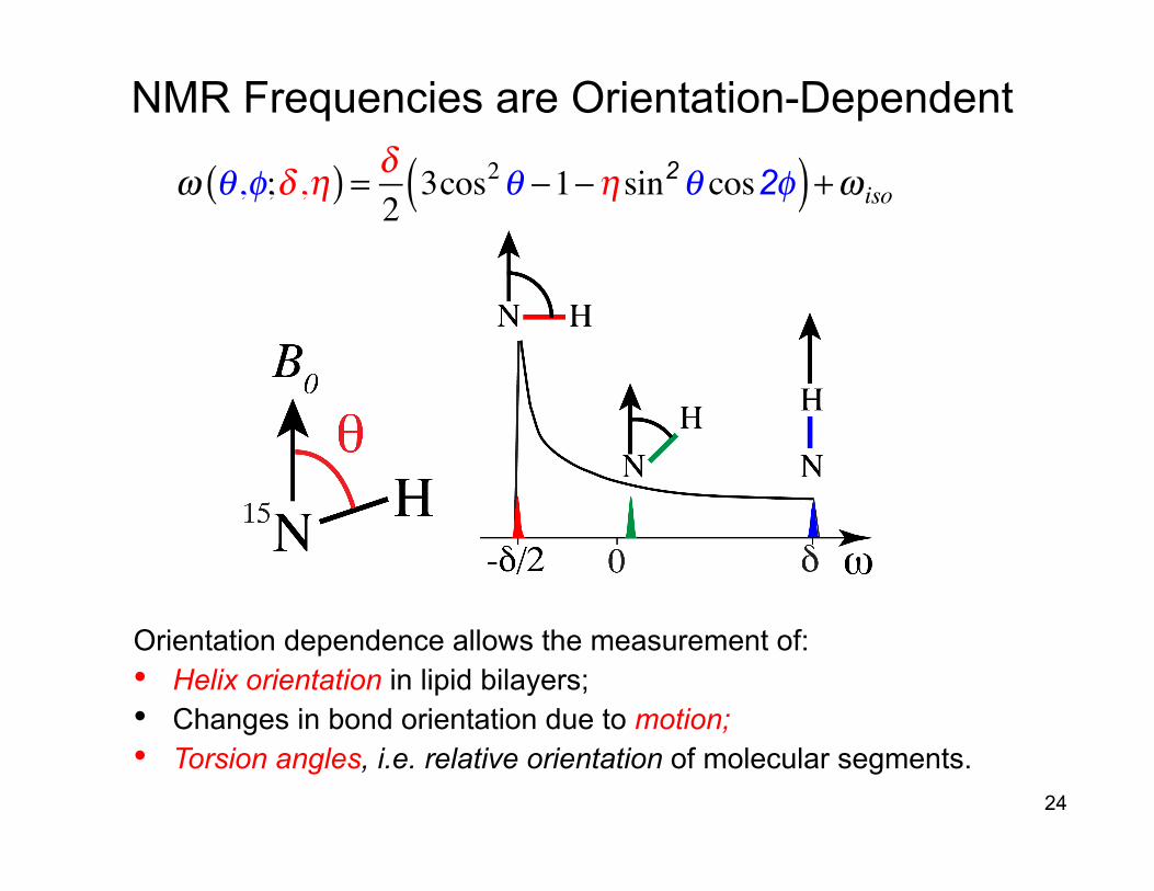
Orientation dependence allows the measurement of: •  Helix orientation in lipid bilayers; •  Changes in bond orientation due to motion; •  Torsion angles, i.e. relative orientation of molecular segments.

NMR Frequencies are Orientation-Dependent

24

ω θ ,φ;δ ,η( ) = δ

23cos2θ −1−η sin2θ cos2φ( ) +ω iso

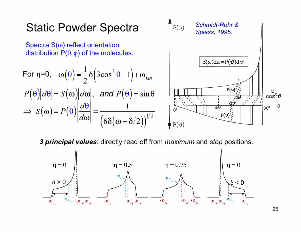
3 principal values: directly read off from maximum and step positions.

P θ( ) dθ = S ω( ) dω , and P θ( ) = sinθ

⇒ S ω( ) = P θ( ) dθdω

= 1

6δ ω + δ 2( )( )1 2

For η=0,

Static Powder Spectra Spectra S(ω) reflect orientation distribution P(θ, ϕ) of the molecules.

ω θ( ) = 1

2δ 3cos2 θ−1( )+ωiso

25

Schmidt-Rohr & Spiess, 1995.

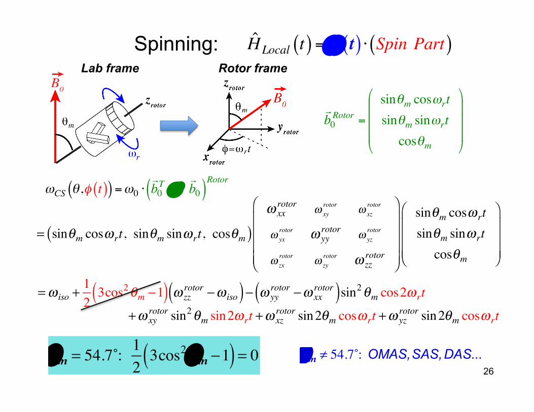
b0Rotor =

sinθm cosωrtsinθm sinωrtcosθm

#

$

%%%

&

'

(((

= sinθm cosω rt, sinθm sinω rt, cosθm( )ω xxrotor ω xy

rotor ω xzrotor

ω yxrotor ω yy

rotor ω yzrotor

ω zxrotor ω zy

rotor ω zzrotor

⎛

⎝

⎜⎜⎜⎜

⎞

⎠

⎟⎟⎟⎟

sinθm cosω rtsinθm sinω rtcosθm

⎛

⎝

⎜⎜⎜

⎞

⎠

⎟⎟⎟

ωCS θ ,φ t( )( ) =ω0 ⋅

b0T σ b0( )

Rotor

Spinning: HLocal t( ) =ω t( ) ⋅ Spin Part( )

θm = 54.7˚: 1

23cos2θm −1( ) = 0 θm ≠ 54.7˚: OMAS, SAS, DAS...

26

=ω iso +123cos2θm −1( ) ω zz

rotor −ω iso( )− ω yyrotor −ω xx

rotor( )sin2θm cos2ω rt

+ω xyrotor sin2θm sin2ω rt +ω xz

rotor sin2θm cosω rt +ω yzrotor sin2θm cosω rt

Lab frame Rotor frame

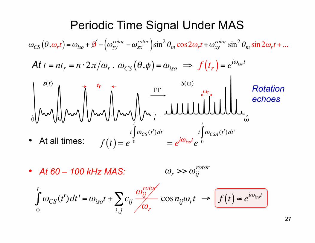
Periodic Time Signal Under MAS

f t( ) = ei ωCS (t' )dt '0

t

∫= eiω isote

i ωCSA (t' )dt '0

t

∫•  At all times:

At t = ntr = n ⋅2π ωr , ωCS θ ,φ( ) =ωiso ⇒ f tr( ) = eiωisot

Rotation echoes

ωCS θ ,ωrt( ) =ωiso + 0 − ωyyrotor −ωxx

rotor( )sin2θm cos2ωrt +ωxyrotor sin2θm sin2ωrt + ...

•  At 60 – 100 kHz MAS: ωr >>ωijrotor

ωCS (t' )dt '

0

t

∫ =ωisot + ciji, j∑

ωijrotor

ωrcosnijωrt → f t( ) ≈ eiωisot

27

28

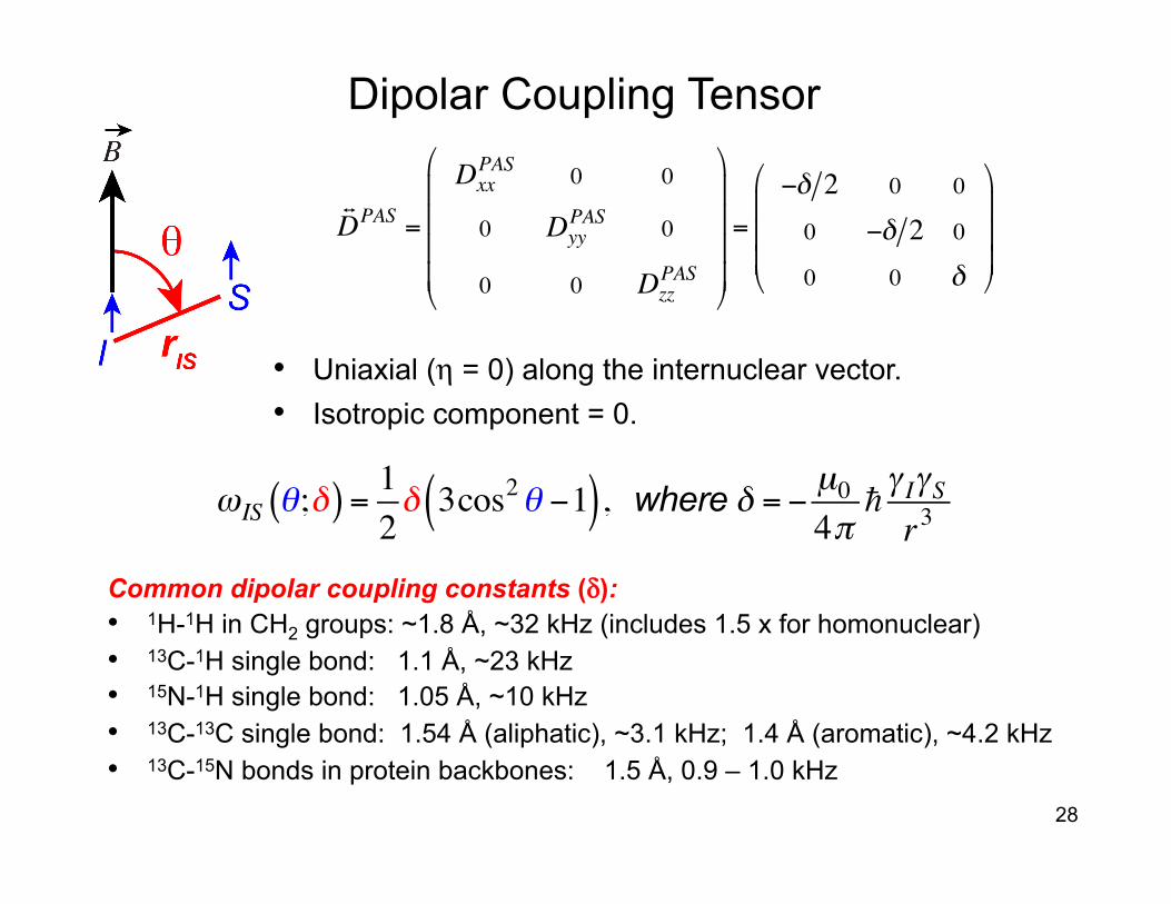
Dipolar Coupling Tensor

DPAS =

DxxPAS 0 0

0 DyyPAS 0

0 0 DzzPAS

!

"

####

$

%

&&&&

=

−δ 2 0 0

0 −δ 2 0

0 0 δ

!

"

###

$

%

&&&

ωIS θ;δ( ) = 1

2δ 3cos2θ −1( ), where δ = − µ0

4πγ IγSr3

•  Uniaxial (η = 0) along the internuclear vector. •  Isotropic component = 0.

Common dipolar coupling constants (δ): •  1H-1H in CH2 groups: ~1.8 Å, ~32 kHz (includes 1.5 x for homonuclear) •  13C-1H single bond: 1.1 Å, ~23 kHz •  15N-1H single bond: 1.05 Å, ~10 kHz •  13C-13C single bond: 1.54 Å (aliphatic), ~3.1 kHz; 1.4 Å (aromatic), ~4.2 kHz •  13C-15N bonds in protein backbones: 1.5 Å, 0.9 – 1.0 kHz

29

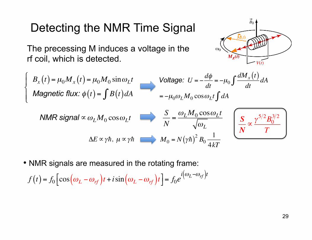
Bx t( ) = µ0Mx t( ) = µ0M0 sinωLt

Magnetic flux: φ t( ) = B t( )dA∫

$

%&

'&

The precessing M induces a voltage in the rf coil, which is detected.

Voltage: U = −dφdt

= −µ0dMx t( )dt

dA∫= −µ0ωLM0 cosωLt dA∫

• NMR signals are measured in the rotating frame:

f t( ) = f0 cos ωL −ωrf( )t + isin ωL −ωrf( )t#$

%&= f0e

i ωL−ωrf( )t

Detecting the NMR Time Signal

M0 = N γ( )2 B0

14kT ΔE∝γ, µ∝γ

SN∝γ 5 2B0

3 2

T NMR signal ∝ωLM0 cosωLt

SN=ωLM0 cosωLt

ωL

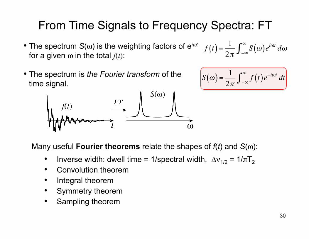
• The spectrum S(ω) is the weighting factors of eiωt for a given ω in the total f(t):

• The spectrum is the Fourier transform of the time signal.

From Time Signals to Frequency Spectra: FT

S ω( ) = 12π

f t( )e−iωt dt−∞

∞∫

f t( ) = 12π

S ω( )eiωt dω−∞

∞∫

Many useful Fourier theorems relate the shapes of f(t) and S(ω): •  Inverse width: dwell time = 1/spectral width, Δν1/2 = 1/πT2 •  Convolution theorem •  Integral theorem •  Symmetry theorem •  Sampling theorem

30