Embed Size (px)
Citation preview
7/28/2019 Bayes SEM. Ferra Et Al 2013
http://slidepdf.com/reader/full/bayes-sem-ferra-et-al-2013 1/17
This article was downloaded by: [Universiti Kebangsaan Malaysia]On: 11 April 2013, At: 00:38Publisher: Taylor & FrancisInforma Ltd Registered in England and Wales Registered Number: 1072954 Registeredoffice: Mortimer House, 37-41 Mortimer Street, London W1T 3JH, UK
Journal of Applied StatisticsPublication details, including instructions for authors and
subscription information:
http://www.tandfonline.com/loi/cjas20
Bayesian structural equation modeling
for the health indexFerra Yanuar
a, Kamarulzaman Ibrahim
b& Abdul Aziz Jemain
b
aDepartment of Mathematics, Faculty of Mathematics and Natural
Sciences, Universitas Andalas, Kampus Limau Manis, 25163,
Padang, Indonesiab
School of Mathematical Sciences, Faculty of Science and
Technology, Universiti Kebangsaan Malaysia, 43600, Bangi,
Selangor, Malaysia
Version of record first published: 04 Apr 2013.
To cite this article: Ferra Yanuar , Kamarulzaman Ibrahim & Abdul Aziz Jemain (2013):
Bayesian structural equation modeling for the health index, Journal of Applied Statistics,
DOI:10.1080/02664763.2013.785491
To link to this article: http://dx.doi.org/10.1080/02664763.2013.785491
PLEASE SCROLL DOWN FOR ARTICLE
Full terms and conditions of use: http://www.tandfonline.com/page/terms-and-conditions
This article may be used for research, teaching, and private study purposes. Anysubstantial or systematic reproduction, redistribution, reselling, loan, sub-licensing,
systematic supply, or distribution in any form to anyone is expressly forbidden.
The publisher does not give any warranty express or implied or make any representationthat the contents will be complete or accurate or up to date. The accuracy of anyinstructions, formulae, and drug doses should be independently verified with primarysources. The publisher shall not be liable for any loss, actions, claims, proceedings,demand, or costs or damages whatsoever or howsoever caused arising directly orindirectly in connection with or arising out of the use of this material.
7/28/2019 Bayes SEM. Ferra Et Al 2013
http://slidepdf.com/reader/full/bayes-sem-ferra-et-al-2013 2/17
Journal of Applied Statistics, 2013
http://dx.doi.org/10.1080/02664763.2013.785491
Bayesian structural equation modeling forthe health index
Ferra Yanuara∗, Kamarulzaman Ibrahimb and Abdul Aziz Jemainb
a Department of Mathematics, Faculty of Mathematics and Natural Sciences, Universitas Andalas, Kampus
Limau Manis, 25163 Padang, Indonesia;b
School of Mathematical Sciences, Faculty of Science and Technology, Universiti Kebangsaan Malaysia, 43600 Bangi, Selangor, Malaysia
( Received 29 September 2010; accepted 11 March 2013)
There are many factors which could influence the level of health of an individual. These factors are
interactive and their overall effects on health are usually measured by an index which is called as health
index. The health index could also be used as an indicator to describe the health level of a community.
Since the health index is important, many research have been done to study its determinant. The main
purpose of this study is to model the health index of an individual based on classical structural equation
modeling (SEM) and Bayesian SEM. For estimation of the parameters in the measurement and structural
equation models, the classical SEM applies the robust-weighted least-square approach, while the BayesianSEM implements the Gibbs sampler algorithm. The Bayesian SEM approach allows the user to use the
prior information for updating the current information on the parameter. Both methods are applied to the
data gathered from a survey conducted in Hulu Langat, a district in Malaysia. Based on the classical and
the Bayesian SEM, it is found that demographic status and lifestyle are significantly related to the health
index. However, mental health has no significant relation to the health index.
Keywords: health index; structural equation modeling; Bayesian SEM;Gibbs sampler; prior information
1. Introduction
The information on the health status of an individual is often gathered based on a health survey.It can be used by decision-makers to allocate resources prudently when planning of activities
which aims at improving the overall health status of a particular community is made. For ease
of interpretation, this information can be summarized in a single value called a health index.
Therefore, it is important to identify the factors that could affect the health index. Various studies
indicate that many factors influence the health index of an individual, including socio-demography,
lifestyle and mental health. Since these influential factors are interrelated and latent because they
cannot be measured directly, it is quite complicated to determine the health index. Consequently,
an appropriate technique which allows for this interrelationship known as the structural equation
∗Corresponding author. Email: [email protected]
© 2013 Taylor & Francis
7/28/2019 Bayes SEM. Ferra Et Al 2013
http://slidepdf.com/reader/full/bayes-sem-ferra-et-al-2013 3/17
2 F. Yanuar et al.
modeling (SEM) has to be applied when estimating the health index. SEM is the statistical tool
which is suitable to be applied for summarizing the health index of an individual.
In this study, the classical SEM is used to construct the model for describing the health index.
SEM has been used by many researchers to analyze a complex phenomenon which involves
hypothesized relationships between independent latent variables and dependent latent variables
[5,13,35]. Since the general goal of SEM is to test the hypothesis that the observed covariancematrix for a set of measured variables is equal to the covariance matrix defined by the hypothesized
model, computational algorithm in SEM is developed on the basis of the sample covariance matrix
S . SEM uses the assumption that the observations are independent and identically distributed
according to the multivariate normal distribution [18]. If this assumption is not fulfilled, the
sample covariance matrix cannot be determined in the usual way and difficult to be obtained [28].
Therefore, many researchers such as Scheines et al. [31], Lee and Shi [19], Ansari et al. [2,3]
and Lee et al. [21] proposed the use of Bayesian approach in SEM to overcome these problems.
This involves the use of Gibbs sampler [12] to obtain samples of arbitrary sizes for summarizing
the posterior distribution for describing the parameters of interest. From these samples, the user
can compute the point estimates, standard deviations and interval estimates for the purpose of making an inference. The Bayesian approach is attractive since it allows the user to use the prior
information for updating the current information regarding the parameters of interest.
The main purpose of this study is to illustrate the value of the classical SEM and the Bayesian
SEM for developing a model which describes the health index of an individual living in Hulu
Langat, Malaysia. The interrelationship among the latent variables such as mental health, socio-
demographic characteristics and lifestyle, and between the latent variables and their respective
manifest variables are determined using the data found from the survey that were undertaken in
Hulu Langat.
2. Data and instrument
The analysis is applied on a data set obtained from the Health Risk Assessment (HRA) survey
that took place in Hulu Langat, a district in Malaysia [9]. The HRA survey was organized by
the Department of Community Health, Medical Faculty, Universiti Kebangsaan Malaysia (UKM)
in collaboration with Hospital Universiti Kebangsaan Malaysia (HUKM) [9] in the year 2001.
HUKM was involved as the main center that coordinated the survey.
The objective of the survey was to promote disease prevention activities and healthy living for
people in the area of Hulu Langat. The data obtained in the HRA survey have also been applied by
Yanuar et al. [37] for constructing the health index. It has to be clarified here that the types of data
involved in their analysis are continuous, binary and ordinal. In this study, however, all the data
considered are of the ordinal type and details on them are given later in this section. Consideringonly one type of data makes the analysis slightly easier. In addition, both the classical and the
Bayesian SEM are applied on the same type of data, making the results found based on the two
approaches comparable. Based on the survey, it is reported that about 5.7% of the people living in
Hulu Langat experiencedhaving three most common diseases which include gastritis, diabetes and
asthma. The data that were provided by 5035 respondents who had given a complete information
required in the survey are considered in the analysis. The respondents eligible to participate in
the survey are those who are 18 years old and older, representing the adult population of Hulu
Langat. The respondents are chosen randomly based on the house visit or consultation in HUKM
between April 2000 and August 2001. The choice of house visit is done randomly based on the
list of household that were available with the enumerators.The information gathered in the survey includes information about lifestyle, socio-demographic
status, mental health condition and biomarkers of individuals living in Hulu Langat. The indicators
used for describing the socio-demographic factor are employment status, education level and age
7/28/2019 Bayes SEM. Ferra Et Al 2013
http://slidepdf.com/reader/full/bayes-sem-ferra-et-al-2013 4/17
Journal of Applied Statistics 3
group [4,8,33,34]. Respondents are asked about their employment status, and the responses are
indicated by 1, 2 and 3 for ‘unemployed’, ‘ordinary’ and ‘professional’, respectively. With respect
to the education level, the responses obtained are coded as 1 as ‘never attend school or attend
elementary school’, 2 as ‘attend high school’ and 3 as ‘attend college/university’. The responses
to employment status are coded as 1, 2 and 3 for ‘unemployed’, ordinary’ and ‘professional’,
respectively. The age of the respondents are classified into three groups which are between 18 and31 years old, between 31 and 56 and more than 56 years old, coded as 1, 2 and 3, respectively.
The indicators for lifestyle as hypothesized in this study are based on the list of health-related
behaviors that have been proposed by several authors. The list of health-related behaviors that has
been suggested by Nakayama et al. [25] is the list that has been used by Boardman [4] andShi [32],
which includes physical exercise, smoking habits, average sleeping hours and average working
hours in a day, is considered in this study. The respondents were asked about their smoking
habits and the responses are coded as 1, 2 and 3 for denoting ‘smoker’, ‘quit’ and ‘non-smoker’,
respectively. Regarding frequency of physical exercise, respondents were asked ‘how many times
a week on the average do you have physical exercise?’ The responses for this question consist of
three categories that are coded as 1, 2 and 3 to indicate ‘none’, ‘1 or 2 times in a week’ and ‘morethan 3 times in a week’, respectively. Working hours in a day are coded into 1 as ‘more than 14 h’,
2 as ‘9–14 h’ and 3 as ‘less than 9 h’. Average sleeping hours in a day are grouped as well, with 1
referring to ‘less than 7 h’, 2 as ‘more than 8 h’ and 3 as ‘7–8 h’.
Nakayama et al. [25] and Boardman [4] have proposed that level of stress, happiness in life
and the number of serious problems that were faced during the last year could be used as the
indicators for mental health. The stress level is divided into three categories which are coded
as 1, 2 and 3, referring to ‘high stress level’, ‘middle’ and ‘normal’, respectively. Happiness in
life is coded into 1 as ‘not happy’, 2 as ‘average’ and 3 as ‘happy’. Meanwhile, the number of
experiences of serious problems during the last year has been categorized into three categories as
well and coded as 1, 2 and 3, referring to ‘having more than 2 problems’, ‘having 1 or 2 problems’
and ‘no problem’, respectively. In addition, medical screening was carried out to measure weight
and height, cholesterol and blood pressure level during consultation at the clinic in the hospital or
during a house visit. The number of health problems that was faced by the respondents are also
asked.
The health index which is assumed to be related to mental health, socio-demography and
lifestyle could also be measured directly based on certain indicators. In this study, the indicators
of the health index are blood pressure, cholesterol level, body mass index (BMI) and the number
of common health problems that the respondent ever had. BMI is defined as the body mass of
an individual divided by the square of his or her height. The values of BMI that are coded as 1,
2 and 3, which denote ‘obese’, ‘risky (underweight or overweight)’ and ‘normal’, respectively,
are based on the guidelines provided by the Centers for Disease Control and Prevention [ 7]. Theclassifications that are made for blood pressure level are ‘high blood pressure’ which is coded as 1,
‘pre-hypertension’ which is coded as 2 and ‘normal’ which is coded as 3, based on the categories
proposed by the American Heart Association [1]. The classifications that are used for the total
cholesterol level consist of three ordered categories as well and decided using the categories
suggested by the National Institutes of Health [26]. Regarding the information on the health level,
the respondents are asked whether they have ever had one or more of the 14 common health
problems considered in the questionnaires of the survey. The respondents who have more than
four health problems are categorized as ‘unhealthy’ and coded as 1, who have two to four health
problems are considered as ‘less healthy’ and coded as 2, and those with fewer than two health
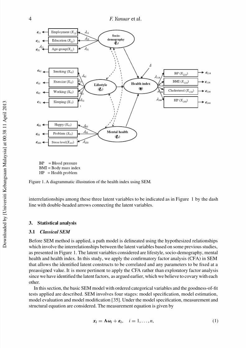
problems are considered as ‘healthy’ and coded as 3.In Figure 1, the hypothesized model which involves measurement and structural components is
used to illustrate the health index model. Since it is also reasonable to hypothesize that lifestyle,
socio-demographic status and mental health are correlated, we suggest that the presence of the
7/28/2019 Bayes SEM. Ferra Et Al 2013
http://slidepdf.com/reader/full/bayes-sem-ferra-et-al-2013 5/17
4 F. Yanuar et al.
Figure 1. A diagrammatic illustration of the health index using SEM.
interrelationships among these three latent variables to be indicated as in Figure 1 by the dash
line with double-headed arrows connecting the latent variables.
3. Statistical analysis
3.1 Classical SEM
Before SEM method is applied, a path model is delineated using the hypothesized relationships
which involve the interrelationships between the latent variables based on some previous studies,
as presented in Figure 1. The latent variables considered are lifestyle, socio-demography, mental
health and health index. In this study, we apply the confirmatory factor analysis (CFA) in SEM
that allows the identified latent constructs to be correlated and any parameters to be fixed at a
preassigned value. It is more pertinent to apply the CFA rather than exploratory factor analysis
since we have identified the latent factors, as argued earlier, which we believe to covary with each
other.
In this section, the basic SEM model with ordered categorical variables and the goodness-of-fit
tests applied are described. SEM involves four stages: model specification, model estimation,
model evaluation and model modification [35]. Under the model specification, measurement and
structural equation are considered. The measurement equation is given by
xi = ωi + εi, i = 1, . . . , n, (1)
7/28/2019 Bayes SEM. Ferra Et Al 2013
http://slidepdf.com/reader/full/bayes-sem-ferra-et-al-2013 6/17
Journal of Applied Statistics 5
where xi is an p × 1 vector of indicators describing the q × 1 random vector of latent variables
ωi, is p × q matrices of the loading coefficients as obtained from the regressions of xi on ωi
and εi is p × 1 random vectors of the measurement errors which follow N (0,ψε). It is assumed
that for i = 1, . . . , n, ωi is independent, follows a normal distribution N (0,) and uncorrelated
with the random vector εi.
Let the latent variable ωi be partitioned into (ηi, ξ i), where ηi and ξ i are m × 1 and n × 1vectors of latent variables, respectively. Equation (2) is the structural equation for explaining the
interrelationship among the latent factors in a form of mathematical expression which is given by
ηi = Bηi + ξ i + δi, i = 1, . . . , n, (2)
where B is m × m matrix of structural parameters governing the relationship among the endoge-
nous latent variables which is assumed to have zeros in the diagonal, is m × n regression
parameter matrix for relating the endogenous latent variables and exogenous latent variables, and
δi is m × 1 vector of disturbances which is assumed N (0,ψδ), where ψδ is a diagonal covariance
matrix. It is also assumed that δi is uncorrelated withξ i. Since only one endogenous latent variableis involved in this study, or Bηi = 0, so Equation (2) can be rewritten as ηi = ξ i + δi.
The second stage of the modeling involves estimation of the parameters specified by the mea-
surement and structural equation models. The aim of the model estimation is to minimize the
difference between the hypothesized matrix and the sample covariance matrix based on a suitable
fitting function. Since non normal and/or non continuous data are considered in this study, robust-
weighted least-square (RWLS) estimation method is an appropriate technique to be utilized. The
analysis based on RWLS provides parameter estimates, standard errors, computed χ 2 and fit
indices which are found using diagonal elements of the weight matrix that are derived from the
asymptotic variances of the thresholds and estimates of the latent correlation [10].
The next process in SEM is the model evaluation of the sample parameters. The criteria for
estimation of fit include examination of the solution, measure of overall fit and detailed assessment
of fit. The first process involved under model evaluation is to check for the appropriateness of each
variable such as the right sign or size of the parameter estimates, correlations between parameter
estimates, the squared multiple correlations or whether or not the ranges of the standard errors fall
within reasonable intervals. The next process is to evaluate the overall model fit by investigating
whether or not the specified model fits the data. A complete discussion of model fit is outside
the scope of this article, thus, emphasis is given on only three most popular fit indices that are
presented by Mplus: the root mean square error of approximation (RMSEA), comparative fit index
(CFI) and Tucker Lewis index (TLI) [14,35]. RMSEA provides a measure of the lack of fit of
a particular model compared with a perfect or saturated model, where the values of 0.06 or less
indicate a good fit, while values larger than 0.10 are an indication of poor fitted models [ 14]. CFIand TLI compare the improvement of the fit of the proposed model over a more restricted model,
called an independence or null model, which specifies no relationships among the variables. The
values of CFI and TLI which are closer to 1.0 (or more than 0.80) indicate the better fitted models
[14]. Mplus also presents the χ 2 and weighted root mean square residual (WRMR). But in this
study, neither of these measures is considered as an indicator of the model fit because the χ 2 test
is sensitive to the sample size and WRMR is an indicator for experimental fit which does not
always behave well.
The last step in SEM is the model modification, a process which is done to improve the fit,
thereby estimating the most likely relationships between variables. Examples of the methods that
could be used in modifying a SEM model are χ
2
difference, Lagrange multiplier (ML) and Waldtests. Many programs provide modification indices that indicate the improvement in fit as the
result of adding an additional path to the model. For the model modification, Mplus applies the
χ 2 difference [35].
7/28/2019 Bayes SEM. Ferra Et Al 2013
http://slidepdf.com/reader/full/bayes-sem-ferra-et-al-2013 7/17
6 F. Yanuar et al.
3.2 Bayesian SEM approach
In this study, the variables gathered are in the form of ordered category. Before conducting the
Bayesian analysis, a threshold specification has to be identified in order to treat the ordered
categorical data as manifestations of hidden continuous normal distribution. Following is a brief
explanation about threshold specification.
Suppose X = ( x1, x2, . . . , x n) and Y = ( y1, y2, . . . , y n) be the ordered categorical data matrices
and latent continuous variables, respectively. The relationship between X and Y is explained by
using the threshold specification as follows. For illustration, consider x1. The same process can
also be done for x2, . . . , x n. Let:
x1 = c if τ c−1 < y1 < τ c, (3)
where c is the number of categories for x1, τ c−1 and τ c denote the threshold levels associated with
y1. For example, in this study, we consider c = 3, where τ 0 = −∞ and τ 3 = ∞. Meanwhile, the
values of τ 1 and τ 2 are determined based on the proportion of cases in each category of x1 using
the formula given by
τ k = −1
2
r =1
N r
N
, k = 1, 2, (4)
where −1(·) is the inverse of the standardized normal distribution, N r is the number of cases in
the r th category and N is the total number of cases. Here, it is assumed that y1 follows a normal
distribution. Thus, we have Y = ( y1, y2, . . . , y n) following a multivariate normal distribution.
Under the Bayesian SEM, we also consider X = ( x1, x2, . . . , x n) and Y = ( y1, y2, . . . , y n)
to be the ordered categorical data matrices and latent continuous variables, respectively, and
= (ω1,ω2, . . . ,ωn) be the matrix of latent variables. The observed data X are augmented with
the latent data (Y ,) in the posterior analysis. In this subsection, we will apply the Bayesianestimation in SEM in order to do posterior analysis to obtain the values of unknown threshold in
τ = (τ 1, τ 2), joint Bayesian estimates of and the structural parameter θ , a vector that includes
all the unknown parameters in , ψδ, ψε, and ω.
The Bayesian method is applied to derive the posterior distribution [τ , θ ,| X ]. The user may
apply maximum likelihood (ML) estimation method to derive the posterior distribution. How-
ever, a high-dimensional integration is required; thus, it is difficult to apply an ML estimation
method in this study [3,19,21]. Thus, the Gibbs sampler algorithm is applied to overcome this
difficulty. The Gibbs sampler is a Markov Chain Monte Carlo (MCMC) technique that generates
a sequence of random observations from the full conditional posterior distribution of unknown
model parameters. The user can create and implement the algorithm easily using winBUGS [33].
Since ordered categorical variables are used, the latent matrix Y should be augmented in the
posterior analysis, resulting in the joint posterior distribution [τ , θ ,, Y | X ]. The Gibbs sampler
process starts with the setting of initial starting values (τ (0), θ (0),(0),Y (0)), and then conduct
the simulation for (τ (1), θ (1),(1), Y (1)). At the r th iteration, by making use of the current values
(τ (r ), θ ( r),( r),Y ( r)), the Gibbs sampler is carried out as follows:
a: Generate ( r+1) from p(|τ (r ), θ ( r),Y ( r), X ),
b: Generate θ ( r+1) from p(θ |( r+1), τ (r ),Y ( r), X ),
c: Generate (τ (r +1),Y ( r+1)) from p(τ , Y |( r+1), θ ( r+1), X ).
Under mild regularity conditions, the samples converge to the desired posterior distribution. The
derivation of the conditional distribution that is required in the Gibbs sampler process is discussed
in Lee and Shi [19] or Lee [18]. In the process when determining the posterior distribution, the
7/28/2019 Bayes SEM. Ferra Et Al 2013
http://slidepdf.com/reader/full/bayes-sem-ferra-et-al-2013 8/17
Journal of Applied Statistics 7
selection of prior distribution for (,ψε) and has to be made. In this study, we take the prior
distribution for those three parameters via the following conjugate type distribution. Letting ψεk
be the k th diagonal element of ψε and k be the k th row of , we consider
ψ −1εk ∼ Gamma(α0εk , β0εk ), (5)
(k |ψ−1εk ) ∼ N (0k , ψεk H0 yk ), (6)
−1 ∼ W q( R0, ρ0), (7)
where Gamma(, ) is the gamma distribution, W q(, ) is an q-dimensional Wishart distribution,
parameters α0εk , β0εk , 0εk , ρ0, positive definite matrix H0 yk and R0 are hyperparameters which
are assumed to be described by an uninformative prior distribution.
The next process in the Bayesian SEM is a convergence test of the model parameters. The
convergence is assessed using a variety of diagnostics as detailed in the CODA package, plotting
the time series to assess the quality of the individual parameters with different starting values
graphically, and provide a diagnosis based on the trace plots [2,16,31]. We also use the Brooks–
Gelman–Rubin convergence statistics [29]. This convergence statistics test compares the variationbetween and within multiple chains, denoted by R. The estimated parameters converge if the value
of R is close to 1. In addition, the accuracy of the posterior estimates are inspected by assuring
that the Monte Carlo error (an estimate of the difference between the mean of the sampled values
and the true posterior mean) for all the parameters to be less than 5% of the sample standard
deviation [6].
For assessing the plausibility of our proposed model which includes the measurement equation
and structural equation, we plot the residual estimates versus latent variable estimates to give
information for the fit of the model. The residuals estimates for measurement equation (ε̂i) can
be obtained from
ε̂i
= yi
− ̂ξ̂ i, i = 1, . . . , n, (8)
where ̂ and ξ̂ i are Bayesian estimates obtained via the MCMC methods. The hypothesized
models provide a good fit if the plots are centered at zero and lie within two parallel horizontal
lines. The estimates of residuals in the structural equation (δ̂i) can be obtained from following
equation:
δ̂i = ( I − ˆ B)η̂i − ̂ξ̂ i, i = 1, . . . , n, (9)
where ˆ B, η̂i, ̂ and ξ̂ i are Bayesian estimates that are obtained from the corresponding simulated
observations through the MCMC. The proposed model fitted the data well or provided a reasonably
good fit if the plots lie within two parallel horizontal lines that are centered at zero and no trends
are detected.
3.3 Modeling description
As given in Figure 1, the hypothesized model in this study consists of 14 indicator variables with
three exogenous latent variables and one endogenous latent variable. The measurement equation
is defined by
yi = ωi + εi, i = 1, . . . , n, (10)
where ωi = (ηi, ξ i1, ξ i2, ξ i3)T. It is assumed that εi is independent, following N (0,ψε ) and
uncorrelated with the latent variable ωi. The structural equation is modeled as follows:
ηi = γ 1ξ i1 + γ 2ξ i2 + γ 3ξ i3 + δi, (11)
where (ξ i1, ξ i2, ξ i3)T is distributed as N (0,) and independent with δi which is distributed as
N (0,ψδ).
7/28/2019 Bayes SEM. Ferra Et Al 2013
http://slidepdf.com/reader/full/bayes-sem-ferra-et-al-2013 9/17
8 F. Yanuar et al.
In the data analysis, we use Mplus version 5.2 [23] to estimate the parameters for the classical
model, while the Bayesian model is fitted to the data using winBUGS version 1.4 [ 33]. The
hierarchical structure is implemented by selecting the prior information for parameters involved
in the hypothesized model as described in Equations (5)–(7).
4. Results
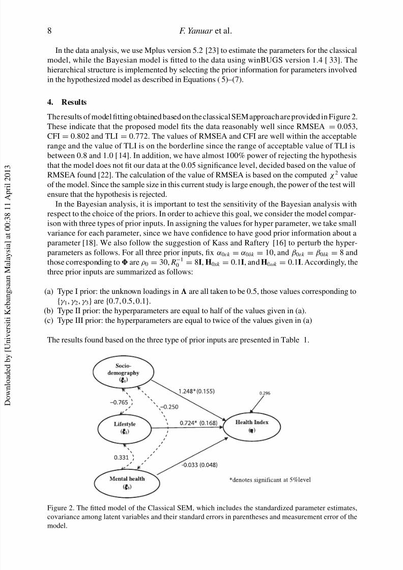
The results of model fitting obtained based on the classical SEM approach are provided in Figure 2.
These indicate that the proposed model fits the data reasonably well since RMSEA = 0.053,
CFI = 0.802 and TLI = 0.772. The values of RMSEA and CFI are well within the acceptable
range and the value of TLI is on the borderline since the range of acceptable value of TLI is
between 0.8 and 1.0 [14]. In addition, we have almost 100% power of rejecting the hypothesis
that the model does not fit our data at the 0.05 significance level, decided based on the value of
RMSEA found [22]. The calculation of the value of RMSEA is based on the computed χ 2 value
of the model. Since the sample size in this current study is large enough, the power of the test will
ensure that the hypothesis is rejected.
In the Bayesian analysis, it is important to test the sensitivity of the Bayesian analysis with
respect to the choice of the priors. In order to achieve this goal, we consider the model compar-
ison with three types of prior inputs. In assigning the values for hyper parameter, we take small
variance for each parameter, since we have confidence to have good prior information about a
parameter [18]. We also follow the suggestion of Kass and Raftery [16] to perturb the hyper-
parameters as follows. For all three prior inputs, fix α0εk = α0δk = 10, and β0εk = β0δk = 8 and
those corresponding to are ρ0 = 30, R−10 = 8I, H0 xk = 0.1I, and H0ωk = 0.1I. Accordingly, the
three prior inputs are summarized as follows:
(a) Type I prior: the unknown loadings in are all taken to be 0.5, those values corresponding to
{γ 1, γ 2, γ 3} are {0.7, 0.5, 0.1}.(b) Type II prior: the hyperparameters are equal to half of the values given in (a).
(c) Type III prior: the hyperparameters are equal to twice of the values given in (a)
The results found based on the three type of prior inputs are presented in Table 1.
Figure 2. The fitted model of the Classical SEM, which includes the standardized parameter estimates,
covariance among latent variables and their standard errors in parentheses and measurement error of the
model.
7/28/2019 Bayes SEM. Ferra Et Al 2013
http://slidepdf.com/reader/full/bayes-sem-ferra-et-al-2013 10/17
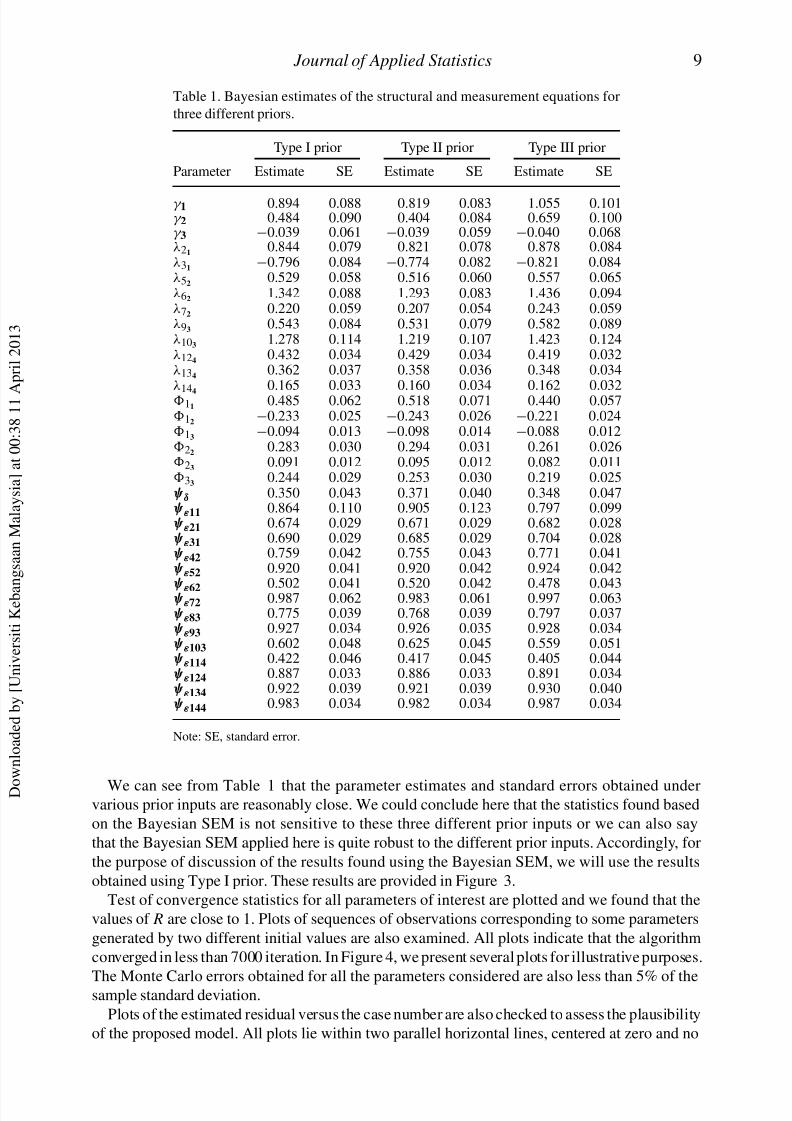
Journal of Applied Statistics 9
Table 1. Bayesian estimates of the structural and measurement equations for
three different priors.
Type I prior Type II prior Type III prior
Parameter Estimate SE Estimate SE Estimate SE
γ 1 0.894 0.088 0.819 0.083 1.055 0.101γ 2 0.484 0.090 0.404 0.084 0.659 0.100γ 3 −0.039 0.061 −0.039 0.059 −0.040 0.068λ21
0.844 0.079 0.821 0.078 0.878 0.084λ31
−0.796 0.084 −0.774 0.082 −0.821 0.084λ52
0.529 0.058 0.516 0.060 0.557 0.065λ62
1.342 0.088 1.293 0.083 1.436 0.094λ72
0.220 0.059 0.207 0.054 0.243 0.059λ93
0.543 0.084 0.531 0.079 0.582 0.089λ103
1.278 0.114 1.219 0.107 1.423 0.124λ124
0.432 0.034 0.429 0.034 0.419 0.032λ134
0.362 0.037 0.358 0.036 0.348 0.034λ
144 0.165 0.033 0.160 0.034 0.162 0.032110.485 0.062 0.518 0.071 0.440 0.057
12−0.233 0.025 −0.243 0.026 −0.221 0.024
13−0.094 0.013 −0.098 0.014 −0.088 0.012
220.283 0.030 0.294 0.031 0.261 0.026
230.091 0.012 0.095 0.012 0.082 0.011
330.244 0.029 0.253 0.030 0.219 0.025
ψδ 0.350 0.043 0.371 0.040 0.348 0.047ψε11 0.864 0.110 0.905 0.123 0.797 0.099ψε21 0.674 0.029 0.671 0.029 0.682 0.028ψε31 0.690 0.029 0.685 0.029 0.704 0.028ψε42 0.759 0.042 0.755 0.043 0.771 0.041ψε52 0.920 0.041 0.920 0.042 0.924 0.042
ψε62 0.502 0.041 0.520 0.042 0.478 0.043ψε72 0.987 0.062 0.983 0.061 0.997 0.063ψε83 0.775 0.039 0.768 0.039 0.797 0.037ψε93 0.927 0.034 0.926 0.035 0.928 0.034ψε103 0.602 0.048 0.625 0.045 0.559 0.051ψε114 0.422 0.046 0.417 0.045 0.405 0.044ψε124 0.887 0.033 0.886 0.033 0.891 0.034ψε134 0.922 0.039 0.921 0.039 0.930 0.040ψε144 0.983 0.034 0.982 0.034 0.987 0.034
Note: SE, standard error.
We can see from Table 1 that the parameter estimates and standard errors obtained undervarious prior inputs are reasonably close. We could conclude here that the statistics found based
on the Bayesian SEM is not sensitive to these three different prior inputs or we can also say
that the Bayesian SEM applied here is quite robust to the different prior inputs. Accordingly, for
the purpose of discussion of the results found using the Bayesian SEM, we will use the results
obtained using Type I prior. These results are provided in Figure 3.
Test of convergence statistics for all parameters of interest are plotted and we found that the
values of R are close to 1. Plots of sequences of observations corresponding to some parameters
generated by two different initial values are also examined. All plots indicate that the algorithm
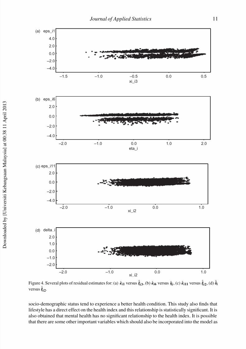
converged in less than 7000 iteration. In Figure 4, we present several plots for illustrative purposes.
The Monte Carlo errors obtained for all the parameters considered are also less than 5% of thesample standard deviation.
Plots of the estimated residual versus the case number are also checked to assess the plausibility
of the proposed model. All plots lie within two parallel horizontal lines, centered at zero and no
7/28/2019 Bayes SEM. Ferra Et Al 2013
http://slidepdf.com/reader/full/bayes-sem-ferra-et-al-2013 11/17
10 F. Yanuar et al.
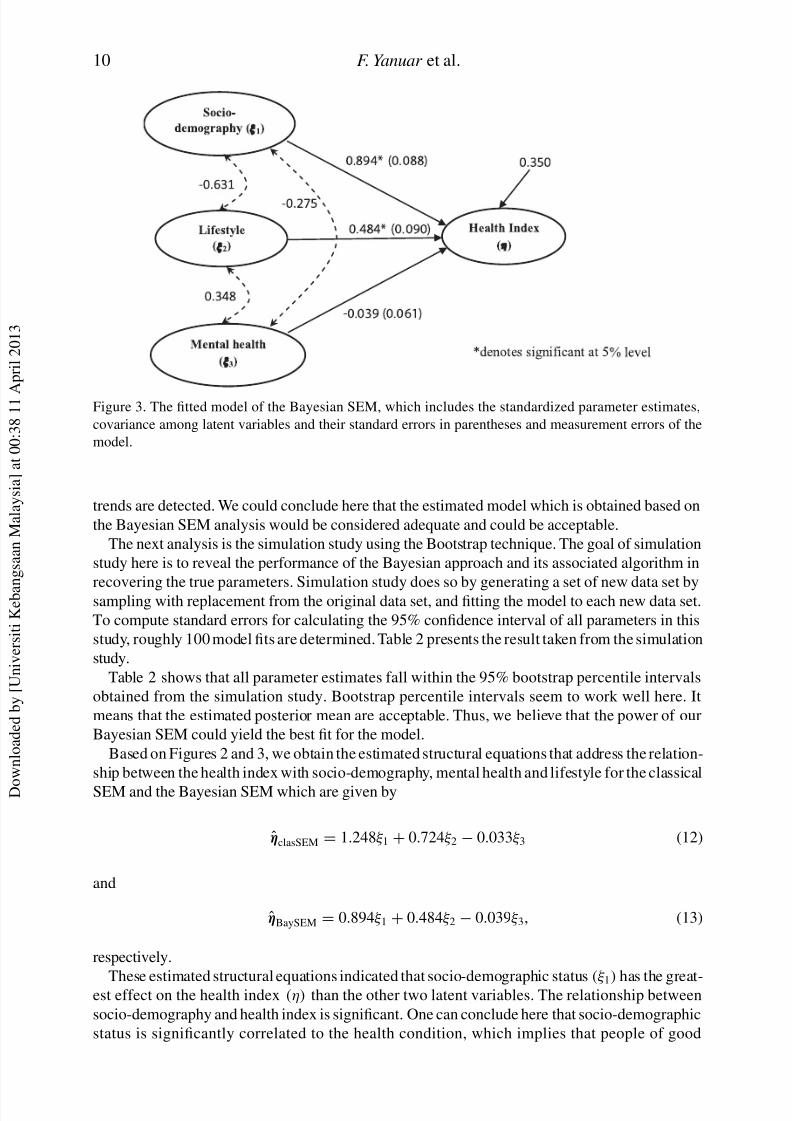
Figure 3. The fitted model of the Bayesian SEM, which includes the standardized parameter estimates,
covariance among latent variables and their standard errors in parentheses and measurement errors of the
model.
trends are detected. We could conclude here that the estimated model which is obtained based on
the Bayesian SEM analysis would be considered adequate and could be acceptable.
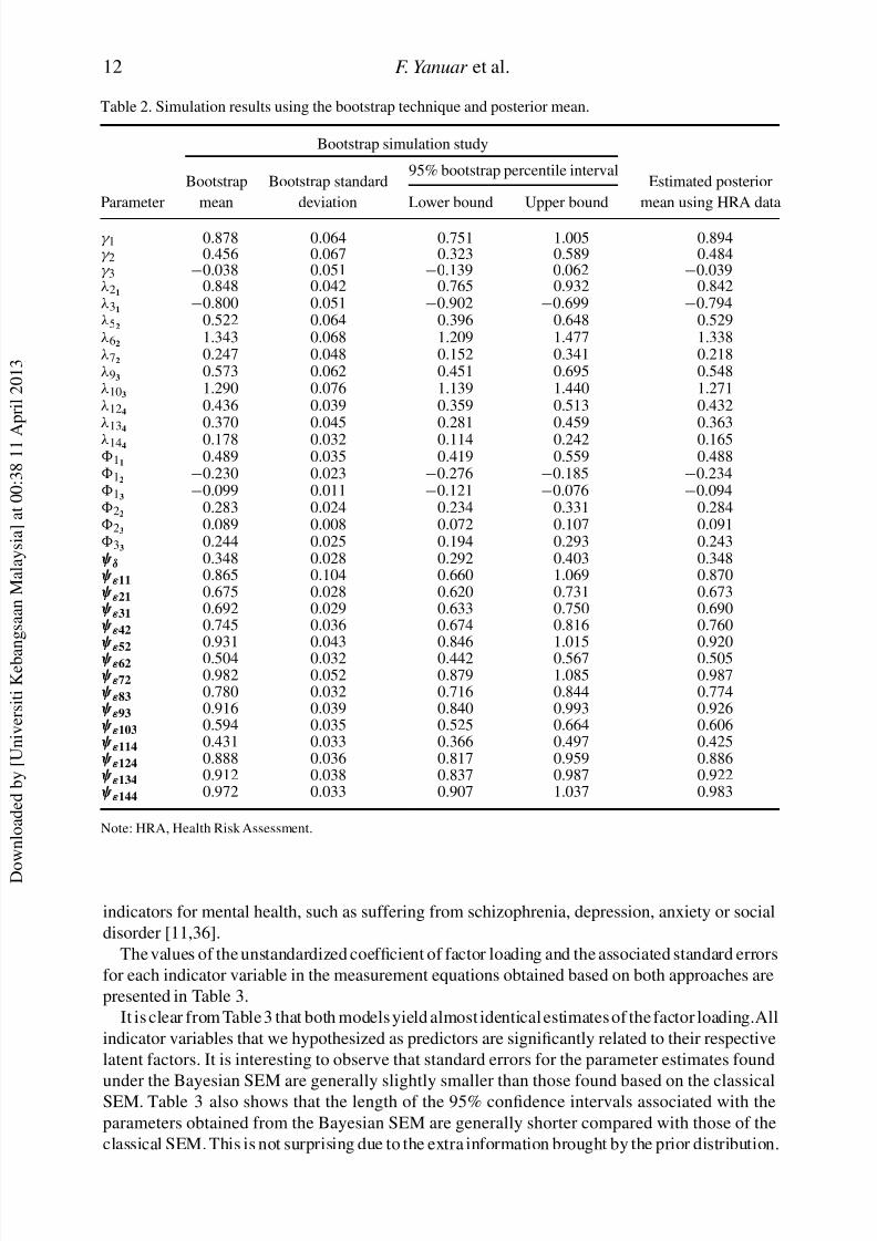
The next analysis is the simulation study using the Bootstrap technique. The goal of simulation
study here is to reveal the performance of the Bayesian approach and its associated algorithm in
recovering the true parameters. Simulation study does so by generating a set of new data set bysampling with replacement from the original data set, and fitting the model to each new data set.
To compute standard errors for calculating the 95% confidence interval of all parameters in this
study, roughly 100 model fits are determined. Table 2 presents the result taken from the simulation
study.
Table 2 shows that all parameter estimates fall within the 95% bootstrap percentile intervals
obtained from the simulation study. Bootstrap percentile intervals seem to work well here. It
means that the estimated posterior mean are acceptable. Thus, we believe that the power of our
Bayesian SEM could yield the best fit for the model.
Based on Figures 2 and 3, we obtain the estimated structural equations that address the relation-
ship between the health index with socio-demography, mental health and lifestyle for the classical
SEM and the Bayesian SEM which are given by
η̂clasSEM = 1.248ξ 1 + 0.724ξ 2 − 0.033ξ 3 (12)
and
η̂BaySEM = 0.894ξ 1 + 0.484ξ 2 − 0.039ξ 3, (13)
respectively.
These estimated structural equations indicated that socio-demographic status (ξ 1) has the great-est effect on the health index (η) than the other two latent variables. The relationship between
socio-demography and health index is significant. One can conclude here that socio-demographic
status is significantly correlated to the health condition, which implies that people of good
7/28/2019 Bayes SEM. Ferra Et Al 2013
http://slidepdf.com/reader/full/bayes-sem-ferra-et-al-2013 12/17
Journal of Applied Statistics 11
xi_i3
–1.5 –1.0 –0.5 0.0 0.5
eps_i1
–4.0
–2.0
0.0
2.0
4.0
(a)
eta_i
–2.0 –1.0 0.0 1.0 2.0
eps_i6
–4.0
–2.0
0.0
2.0
(b)
xi_i2 –2.0 –1.0 0.0 1.0
eps_i11
–4.0
–2.0
0.0
2.0
(c)
xi_i2 –2.0 –1.0 0.0 1.0
delta_i
–2.0
–1.0
0.0
1.0
2.0
(d)
Figure 4. Several plots of residual estimates for: (a) ε̂i1 versus ξ̂ i3, (b) ε̂i6 versus η̂i, (c) ε̂i11 versus ξ̂ i2, (d) δ̂i
versus ξ̂ i2.
socio-demographic status tend to experience a better health condition. This study also finds thatlifestyle has a direct effect on the health index and this relationship is statistically significant. It is
also obtained that mental health has no significant relationship to the health index. It is possible
that there are some other important variables which should also be incorporated into the model as
7/28/2019 Bayes SEM. Ferra Et Al 2013
http://slidepdf.com/reader/full/bayes-sem-ferra-et-al-2013 13/17
12 F. Yanuar et al.
Table 2. Simulation results using the bootstrap technique and posterior mean.
Bootstrap simulation study
95% bootstrap percentile intervalBootstrap Bootstrap standard Estimated posterior
Parameter mean deviation Lower bound Upper bound mean using HRA data
γ 1 0.878 0.064 0.751 1.005 0.894γ 2 0.456 0.067 0.323 0.589 0.484γ 3 −0.038 0.051 −0.139 0.062 −0.039λ21
0.848 0.042 0.765 0.932 0.842λ31
−0.800 0.051 −0.902 −0.699 −0.794λ52
0.522 0.064 0.396 0.648 0.529λ62
1.343 0.068 1.209 1.477 1.338λ72
0.247 0.048 0.152 0.341 0.218λ93
0.573 0.062 0.451 0.695 0.548λ103
1.290 0.076 1.139 1.440 1.271λ124
0.436 0.039 0.359 0.513 0.432λ134
0.370 0.045 0.281 0.459 0.363
λ144 0.178 0.032 0.114 0.242 0.16511
0.489 0.035 0.419 0.559 0.48812
−0.230 0.023 −0.276 −0.185 −0.23413
−0.099 0.011 −0.121 −0.076 −0.09422
0.283 0.024 0.234 0.331 0.28423
0.089 0.008 0.072 0.107 0.09133
0.244 0.025 0.194 0.293 0.243ψδ 0.348 0.028 0.292 0.403 0.348ψε11 0.865 0.104 0.660 1.069 0.870ψε21 0.675 0.028 0.620 0.731 0.673ψε31 0.692 0.029 0.633 0.750 0.690ψε42 0.745 0.036 0.674 0.816 0.760ψε52
0.931 0.043 0.846 1.015 0.920ψε62 0.504 0.032 0.442 0.567 0.505ψε72 0.982 0.052 0.879 1.085 0.987ψε83 0.780 0.032 0.716 0.844 0.774ψε93 0.916 0.039 0.840 0.993 0.926ψε103 0.594 0.035 0.525 0.664 0.606ψε114 0.431 0.033 0.366 0.497 0.425ψε124 0.888 0.036 0.817 0.959 0.886ψε134 0.912 0.038 0.837 0.987 0.922ψε144 0.972 0.033 0.907 1.037 0.983
Note: HRA, Health Risk Assessment.
indicators for mental health, such as suffering from schizophrenia, depression, anxiety or social
disorder [11,36].
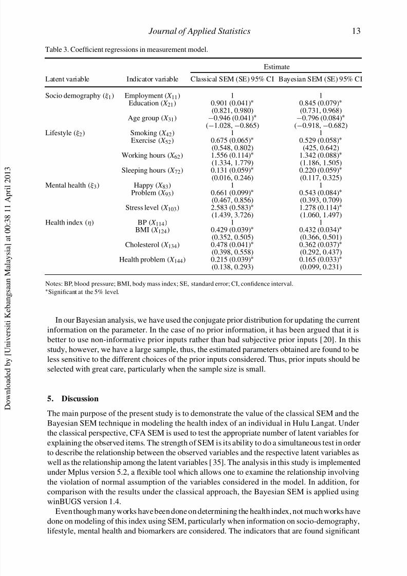
The values of the unstandardized coefficient of factor loading and the associated standard errors
for each indicator variable in the measurement equations obtained based on both approaches are
presented in Table 3.
It is clear from Table 3 that both models yield almost identical estimates of the factor loading.All
indicator variables that we hypothesized as predictors are significantly related to their respective
latent factors. It is interesting to observe that standard errors for the parameter estimates found
under the Bayesian SEM are generally slightly smaller than those found based on the classicalSEM. Table 3 also shows that the length of the 95% confidence intervals associated with the
parameters obtained from the Bayesian SEM are generally shorter compared with those of the
classical SEM. This is not surprising due to the extra information brought by the prior distribution.
7/28/2019 Bayes SEM. Ferra Et Al 2013
http://slidepdf.com/reader/full/bayes-sem-ferra-et-al-2013 14/17
Journal of Applied Statistics 13
Table 3. Coefficient regressions in measurement model.
Estimate
Latent variable Indicator variable Classical SEM (SE) 95% CI Bayesian SEM (SE) 95% CI
Socio demography (ξ 1) Employment ( X 11) 1 1Education ( X 21) 0.901 (0.041)∗ 0.845 (0.079)∗
(0.821, 0.980) (0.731, 0.968)Age group ( X 31) −0.946 (0.041)∗ −0.796 (0.084)∗
(−1.028, −0.865) (−0.918, −0.682)Lifestyle (ξ 2) Smoking ( X 42) 1 1
Exercise ( X 52) 0.675 (0.065)∗ 0.529 (0.058)∗
(0.548, 0.802) (425, 0.642)Working hours ( X 62) 1.556 (0.114)∗ 1.342 (0.088)∗
(1.334, 1.779) (1.186, 1.505)Sleeping hours ( X 72) 0.131 (0.059)∗ 0.220 (0.059)∗
(0.016, 0.246) (0.117, 0.325)Mental health (ξ 3) Happy ( X 83) 1 1
Problem ( X 93) 0.661 (0.099)∗ 0.543 (0.084)∗
(0.467, 0.856) (0.393, 0.709)Stress level ( X 103) 2.583 (0.583)∗ 1.278 (0.114)∗
(1.439, 3.726) (1.060, 1.497)Health index (η) BP ( X 114) 1 1
BMI ( X 124) 0.429 (0.039)∗ 0.432 (0.034)∗
(0.352, 0.505) (0.366, 0.501)Cholesterol ( X 134) 0.478 (0.041)∗ 0.362 (0.037)∗
(0.398, 0.558) (0.292, 0.437)Health problem ( X 144) 0.215 (0.039)∗ 0.165 (0.033)∗
(0.138, 0.293) (0.099, 0.231)
Notes: BP, blood pressure; BMI, body mass index; SE, standard error; CI, confidence interval.∗Significant at the 5% level.
In our Bayesian analysis, we have used the conjugate prior distribution for updating the current
information on the parameter. In the case of no prior information, it has been argued that it is
better to use non-informative prior inputs rather than bad subjective prior inputs [20]. In this
study, however, we have a large sample, thus, the estimated parameters obtained are found to be
less sensitive to the different choices of the prior inputs considered. Thus, prior inputs should be
selected with great care, particularly when the sample size is small.
5. Discussion
The main purpose of the present study is to demonstrate the value of the classical SEM and the
Bayesian SEM technique in modeling the health index of an individual in Hulu Langat. Under
the classical perspective, CFA SEM is used to test the appropriate number of latent variables for
explaining the observed items. The strength of SEM is its ability to do a simultaneous test in order
to describe the relationship between the observed variables and the respective latent variables as
well as the relationship among the latent variables [35]. The analysis in this study is implemented
under Mplus version 5.2, a flexible tool which allows one to examine the relationship involving
the violation of normal assumption of the variables considered in the model. In addition, for
comparison with the results under the classical approach, the Bayesian SEM is applied using
winBUGS version 1.4.Even though many works have been done on determining the health index, not much works have
done on modeling of this index using SEM, particularly when information on socio-demography,
lifestyle, mental health and biomarkers are considered. The indicators that are found significant
7/28/2019 Bayes SEM. Ferra Et Al 2013
http://slidepdf.com/reader/full/bayes-sem-ferra-et-al-2013 15/17
14 F. Yanuar et al.
in explaining the latent factors considered in this study are as follows. The socio-demographic
indicators are employment status, education level and age-group. Lifestyle is explained using
smoking habit, frequency of engaging in physical exercise, number of working hours and number
of sleeping hours. Stress levels, how do the respondent feel about her /his life and experience of
serious problems that respondents have, are used as indicators to measure mental health condition.
This study found that socio-demography and lifestyle have a significant effect on the health index,but mental health does not. These findings are similar to the study of Rizal [30], who indicated
that hypertension, which he considered as an indicator of a health index, is significantly related to
indicators of socio-demography, such as age, education level, employment status and indicators of
lifestyle, i.e. smoking habit andexercise. He also finds that mental healthdoes not have a significant
effect on the health index. This result is similar to the study of Jamsiah et al. [15], which found that
hypertension have no association with stress, which they believe to be an indicator of mental health.
However, some studies found that mental health is significantly related to the health index
[24]. This conflicting evidence between this study and some other previous studies could possibly
be due to the choice of indicators used to explain mental health. Some studies have considered
schizophrenia, depression and anxiety for describing mental health [11,36]. However, for themajority of Malaysians, we believe, and it remains to be investigated, that it is uncalled-for in our
society for someone to admit of having a mental disease such as schizophrenia because having
schizophrenia is associated with being insane and people that are insane have no place in the
society. Accordingly, distant proxies such as the level of stress experienced by the respondents
have been used in this study instead of medical diagnoses as indicators of mental health. In
addition, the studies by Nakayama et al. [25] and Nagano et al. [24], which were carried out in
the factories indicate that the Japanese workers who used to work overtime have a high level of
stress, implying that long working hours contribute a negative impact on mental health. Thus,
length of working hours is another factor which could possibly be considered as an indicator for
mental health.
It is envisaged that factors such as living environment, food consumption and length of working
hours should also be considered when modeling the health index. The study conducted by Kiyu
et al. [17] in Sarawak, for example, has identified that smoking habit, exercise habit and living
environment are factors that are significant in determining the level of health. Noor [27] has
indicated in his work that food consumption and lifestyle play an important role in influencing
the level of health of an individual. Certainly, many other factors in addition to these three factors
could possibly influence a person’s health condition.
The idea of modeling the health index by considering various indicators which describe the
latent factors could further be explored by incorporating new HRA survey data. This idea is
particularly suitable under the sequential Bayesian approach by considering results of this study
as the prior input for the new survey. In this way, at least to some extent, the current health statusof individual living in Hulu Langat can be monitored.
Acknowledgements
The authors thank the Associate Professor Khalib A Latiff and Mr Khairul Yusof from the Department of Community
Health, Medical Faculty, UKM, who furnished us the health survey data used in this study. This research was financially
supported by Directorate General of Higher Education, Ministry of National Education, Indonesia. In addition, a partial
support was also obtained from UKM under the research grant with the code UKM-ST-06-FRGS0011-2007. We also
thank several anonymous referees for their constructive comments which have improved the final version of this paper.
References
[1] American Heart Association, What is High Blood Pressure?, 2008. Available at http://www.americanheart.org/
presenter.jhtml?identifier=2112.
7/28/2019 Bayes SEM. Ferra Et Al 2013
http://slidepdf.com/reader/full/bayes-sem-ferra-et-al-2013 16/17
Journal of Applied Statistics 15
[2] A. Ansari, K. Jedidi, and L. Dube, Heterogeneous factor analysis models: A Bayesian approach, Psychometrika
67 (2002), pp. 49–78.
[3] A. Ansari, K. Jedidi, and S. Jagpal, A hierarchical Bayesian methodology for treating heterogeneity in structural
equation models, Market. Sci. 19 (2000), pp. 328–347.
[4] J.D. Boardman, Stress and physical health: The role of neighborhoods as mediating and moderating mechanisms,
Soc. Sci. Med. 58 (2004), pp. 2473–2483.
[5] D.R. Boniface and M.E. Tefft, The application of structural equation modeling to the construction of a index for themeasurement of health-related behaviours, The Stat. 46 (1997), pp. 505–514.
[6] S.P. Brooks and A. Gelman, Alternative methods for monitoring convergence of iteration simulations, J. Comput.
Graph. Statist. 7 (1998), pp. 434–455.
[7] Centers for Disease Control and Prevention, About BMI for adults, preprint (2009). Available at
http://www.cdc.gov/healthyweight/assessing/bmi/adult_bmi/index.html.
[8] A. Cheadle, D. Pearson, E. Wagner, B.M. Psaty, P. Diehr, and T. Koepsell, Relationship between socioeconomic
status, health status, and lifestyle practices of American Indians: Evidence from a plains reservation population,
Public Health Report 109 (1994), pp. 405–413.
[9] Department of Community Health, Medical Faculty, Universiti Kebangsaan Malaysia, Health risk assessment of
Hulu Langat District , UKM Press, Bangi, Malaysia, 2002.
[10] D.B. Flora and P.J. Curran, An empirical evaluation of alternative methods of estimation for confirmatory factor
analysis with ordinal data, Psychol. Methods 4 (2004), pp. 466–491.
[11] D. Freeman, D. Stahl, S. McManus, H. Melzer, T. Brugha, N. Wiles, and P. Bebbington, Insomnia, worry, anxiety
and depression as predictors of the occurrence and persistence of paranoid thinking, Soc. Psychiatry. Psychiatr.
Epidemiol. 47 (2012), pp. 1195–1203.
[12] G. Geman and D. Geman, Stochastic relaxation, Gibbs distributions, and the Bayesian restoration of images, IEEE
Trans. Pattern Anal. Mach. Intell. 6 (1984), pp. 721–741.
[13] R.S. Hesketh and A. Skrondal, Classical latent variable models for medical research, Stat. Methods Med. Res.
17 (2008), pp. 5–32.
[14] L. Hu and P.M. Bentler, Cutoff criteria for fit indexes in covariance structure analysis: Conventional criteria versus
new alternatives, Struct. Equ. Model. 6 (1999), pp. 1–55.
[15] M. Jamsiah, S.S. Rosnah, and H.I. Noor, Stress in adult population in the suburbs of Hulu Langat, Selangor ,
J. Community Health. 16 (2010), pp. 12–16 (In Malay).
[16] R.E. Kass and A.E. Raftery, Bayes factors, J. Amer. Statist. Assoc. 90 (1995), pp. 773–795.
[17] A. Kiyu, A. Ashley, B. Steinkuehler, J. Hashim, J. Hall, F.S. Peter, W. Lee, and R. Taylor, Evaluation of the healthyvillage program in Kapit District, Sarawak, Malaysia, Health Promot. Int. 21 (2006), pp. 13–18.
[18] S.Y. Lee, Structural Equation Modeling: A Bayesian Approach, John Wiley & Sons, Ltd., New York, 2007.
[19] S.Y. Lee and J.Q. Shi, Bayesian analysis of structural equation model with fixed covariates, Struct. Equ. Model.
7 (2000), pp. 411–430.
[20] S.Y. Lee and X.Y. Song, Evaluation of the Bayesian and maximum likelihood approaches in analyzing structural
equation models with small sample sizes, Multivar. Behav. Res. 39 (2004), pp. 653–686.
[21] S.Y. Lee, X.Y. Song, S. Skeviton, and Y.T. Hao, Application of structural equation models to quality of life, Struct.
Equ. Model. 12 (2005), pp. 435–453.
[22] R.C. MacCallum, M.W. Browne, and H.H. Sugawara, Poweranalysisand determination of sample sizefor covariance
structure modeling, Psychol. Method. 1 (1996), pp. 130–149.
[23] L.K. Muthén and B.O Muthén, Mplus User’s Guide, 5th ed., Muthén & Muthén, Los Angeles, CA, 2007.
[24] C. Nagano, R. Etoh, N. Honda, R. Fujii, N. Sasaki,Y. Kawase,T. Tsutsui, and S. Horie, Association of overtime-work hours with lifestyle and mental health status, Int. Congr. Ser. 1294 (2006), pp. 190–193.
[25] K. Nakayama, K. Yamaguchi, S. Maruyama, and K. Morimoto, The relationship of lifestyle factors, personal char-
acter, and mental health status of employees of a major Japanese electrical manufacturer , Environ. Health Prevent.
Med. 5 (2001), pp. 144–149.
[26] National Institutes of Health, National Heart, Lung, and Blood Institute, ATP III Guidelines At-A-Glance. Quick
Desk Reference, NIH publication No. 01-3305, 2001. Available at http://www.nhlbi.nih.gov/guidelines/cholesterol/
atglance.pdf.
[27] M.I. Noor, The nutrition and health transition in Malaysia, Public Health Nutrition 5 (2002), pp. 191–195.
[28] U.H. Olsson, T. Foss, S.V. Troye, and R.D. Howell, The performance of ML, GLS, and WLS estimation in SEM
under conditions of misspecification and non-normality, Struct. Equ. Model. 7 (2000), pp. 557–595.
[29] J. Palomo, D.B. Dunson, and K. Bollen, Bayesian structural equation modeling, Handb. Comput. Stat. Appl. 1
(2007), pp. 163–188.
[30] A.M. Rizal, The study of the prevalence of the level of knowledge, attitudes and hypertension practices and factors
effecting them among the residents in Kampung Batu 5, Semenyih, Selangor , Jurnal Kesihatan Masyarakat 7 (2001),
pp. 57–62 (In Malay).
7/28/2019 Bayes SEM. Ferra Et Al 2013
http://slidepdf.com/reader/full/bayes-sem-ferra-et-al-2013 17/17
16 F. Yanuar et al.
[31] R. Scheines, H. Hoijtink, and A. Boomsma, Bayesian estimation and testing of structural equation models,
Psychometrika 64 (1999), pp. 37–52.
[32] L. Shi, Socio-demography characteristics and individual health behaviors, Socio Demograph. Factors Health Behav.
91 (1998), pp. 933–942.
[33] D. Spiegelhalter, A. Thomas, N. Best, and D. Lunn, WinBUGS User Manual, Version 1.4, 2003. Available at
http://www.mrc-bsu.cam.ac.uk/bugs.
[34] D.G. Uitenbroek, A. Kerekovska, and N. Festchieva, Health lifestyle behaviour and socio-demography characteris-tics. A study of Varna, Glasgow and Edinburgh, Soc. Sci. Med. 43 (1996), pp. 367–377.
[35] J.B. Ullman, Structural equation modeling: Reviewing the basics and moving forward , J. Pers. Assess. 87 (2006),
pp. 35–50.
[36] WebMD, Mental Health and Schizophrenia. Available at http://www.webmd.com/schizophrenia/guide/mental-
health-schizophrenia.
[37] F. Yanuar, K. Ibrahim, and A.A. Jemain, On the application of structural equation modeling for the construction of
a health index , Environ. Health Prevent. Med. 15 (2010), pp. 285–291.