Embed Size (px)
Citation preview

1
Bayesian Network Meta-Analysis
in BUGS
21 January 2016
Thi Minh Thao HUYNH
Methods & Analytic – global HEOR – SANOFI
JGEM‐SFES
BUGS: Bayesian Inference Using Gibbs Sampling
2 2
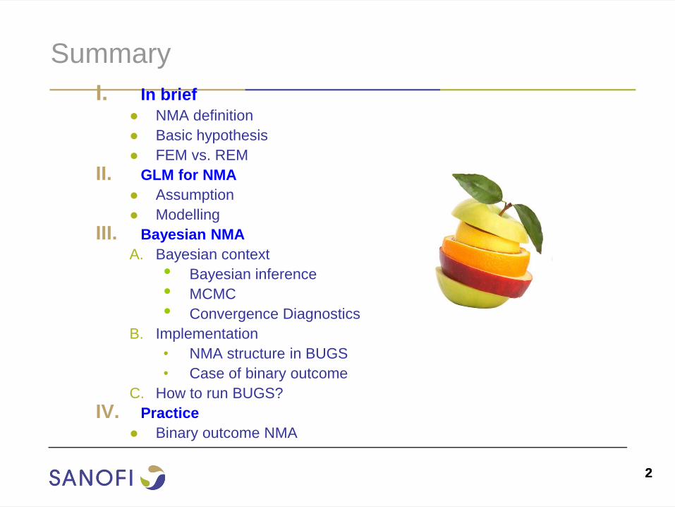
Summary
I. In brief
● NMA definition
● Basic hypothesis
● FEM vs. REM
II. GLM for NMA
● Assumption
● Modelling
III. Bayesian NMA
A. Bayesian context
• Bayesian inference
• MCMC
• Convergence Diagnostics
B. Implementation
• NMA structure in BUGS
• Case of binary outcome
C. How to run BUGS?
IV. Practice
● Binary outcome NMA

3 3
I. In brief
● NMA definition
● Basic hypotheses
● FEM vs. REM
4 4
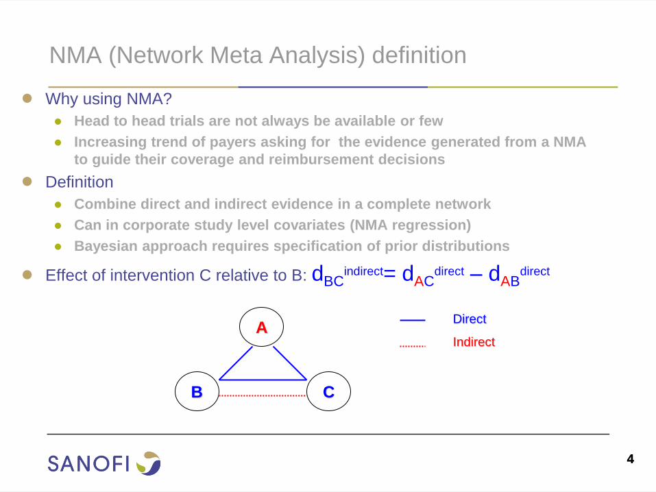
NMA (Network Meta Analysis) definition
● Why using NMA?
● Head to head trials are not always be available or few
● Increasing trend of payers asking for the evidence generated from a NMA
to guide their coverage and reimbursement decisions
● Definition
● Combine direct and indirect evidence in a complete network
● Can in corporate study level covariates (NMA regression)
● Bayesian approach requires specification of prior distributions
● Effect of intervention C relative to B: dBCindirect= dAC
direct – dABdirect
A
B C
Direct
Indirect
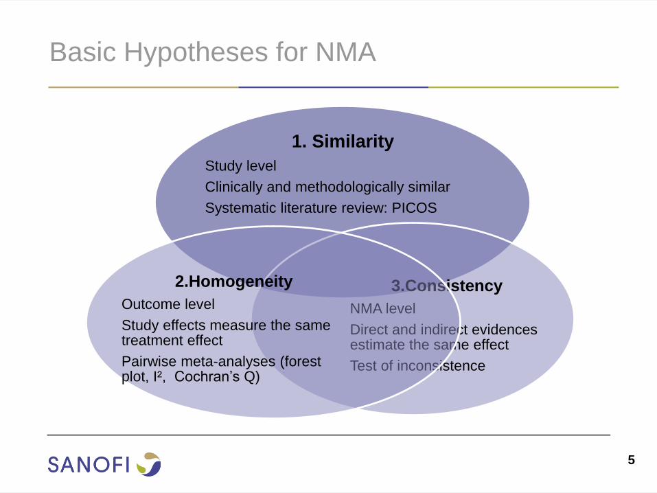
Basic Hypotheses for NMA
1. Similarity
Study level
Clinically and methodologically similar
Systematic literature review: PICOS
3.Consistency
NMA level
Direct and indirect evidences estimate the same effect
Test of inconsistence
2.Homogeneity
Outcome level
Study effects measure the same treatment effect
Pairwise meta-analyses (forest plot, I², Cochran’s Q)
5
6 6
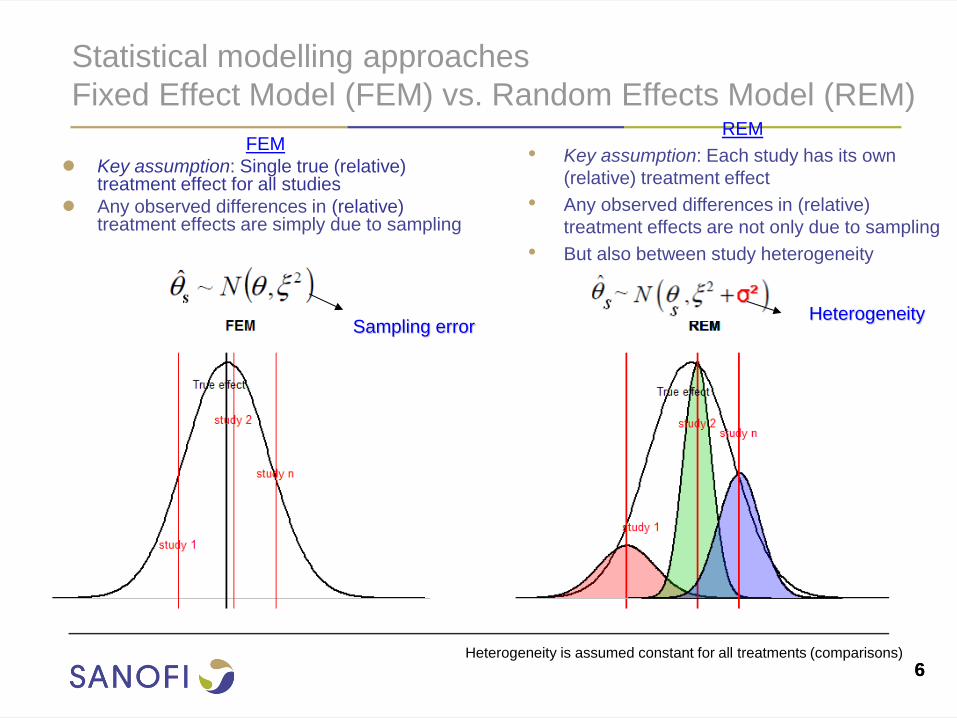
Statistical modelling approaches
Fixed Effect Model (FEM) vs. Random Effects Model (REM)
FEM
● Key assumption: Single true (relative) treatment effect for all studies
● Any observed differences in (relative) treatment effects are simply due to sampling
REM
• Key assumption: Each study has its own
(relative) treatment effect
• Any observed differences in (relative)
treatment effects are not only due to sampling
• But also between study heterogeneity
Heterogeneity Sampling error
Heterogeneity is assumed constant for all treatments (comparisons)

7 7
II. GLM for NMA
● Assumption
● Modelling
● Idea
● Likelihood
● Model(GLM)
8 8
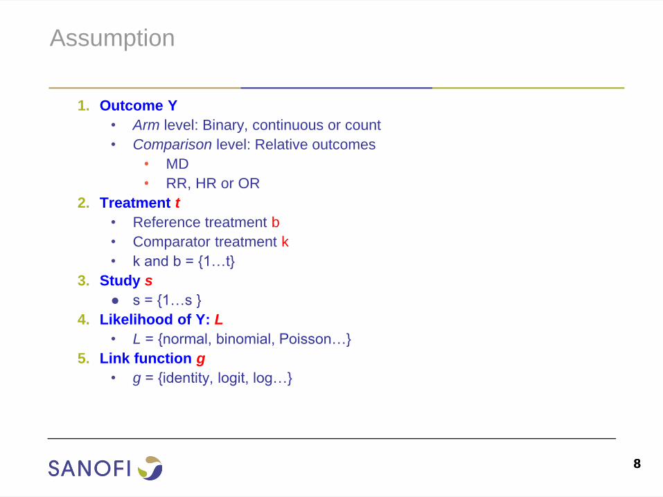
Assumption
1. Outcome Y
• Arm level: Binary, continuous or count
• Comparison level: Relative outcomes
• MD
• RR, HR or OR
2. Treatment t
• Reference treatment b
• Comparator treatment k
• k and b = {1…t}
3. Study s
● s = {1…s }
4. Likelihood of Y: L
• L = {normal, binomial, Poisson…}
5. Link function g
• g = {identity, logit, log…}
9 9
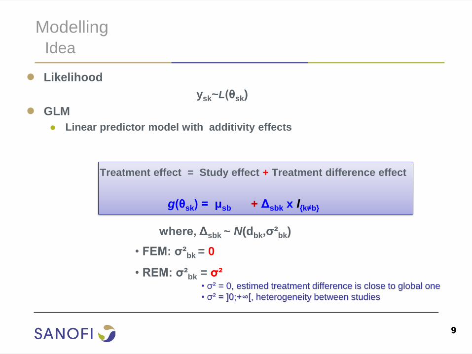
Modelling
Idea
● Likelihood
ysk~L(θsk)
● GLM
● Linear predictor model with additivity effects
Treatment effect = Study effect + Treatment difference effect
g(θsk) = μsb + Δsbk x Ι{k≠b}
where, Δsbk ~ N(dbk,σ²bk)
• FEM: σ²bk = 0
• REM: σ²bk = σ² • σ² = 0, estimed treatment difference is close to global one
• σ² = ]0;+∞[, heterogeneity between studies
10 10
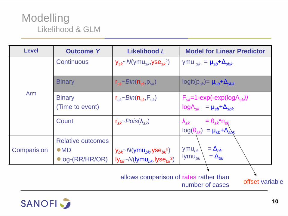
Modelling Likelihood & GLM
Level Outcome Y Likelihood L Model for Linear Predictor
Arm
Continuous ysk~N(ymusk,ysesk²)
ymu sk = μsb+Δsbk
Binary rsk~Bin(nsk,psk) logit(psk)= μsb+Δsbk
Binary
(Time to event)
rsk~Bin(nsk,Fsk) Fsk=1-exp(-exp(logΛsk))
logΛsk = μsb+Δsbk
Count rsk~Pois(λsk) λsk = θsk*nsk
log(θsk) = μsb+Δsbk
Comparision
Relative outcomes
●MD
●log-(RR/HR/OR)
ybk~N(ymubk,ysebk²)
lybk~N(lymubk,lysebk²)
ymubk = Δbk
lymubk = Δbk
allows comparison of rates rather than
number of cases offset variable
II. NMA with Bayesian approach
A. Bayesian context
• Bayesian inference
• MCMC Simulation
• Convergence Diagnostic
B. Implementation
• NMA structure in BUGS
• Case of binary outcome
C. How to run WinBUGS?
11 11
12 12
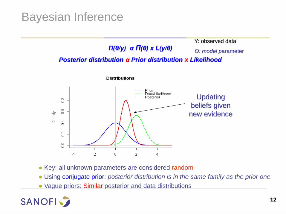
Bayesian Inference
Π(θ/y) α Π(θ) x L(y/θ)
Posterior distribution α Prior distribution x Likelihood
● Key: all unknown parameters are considered random
● Using conjugate prior: posterior distribution is in the same family as the prior one
● Vague priors: Similar posterior and data distributions
Y: observed data
Θ: model parameter
Updating
beliefs given
new evidence
13 13
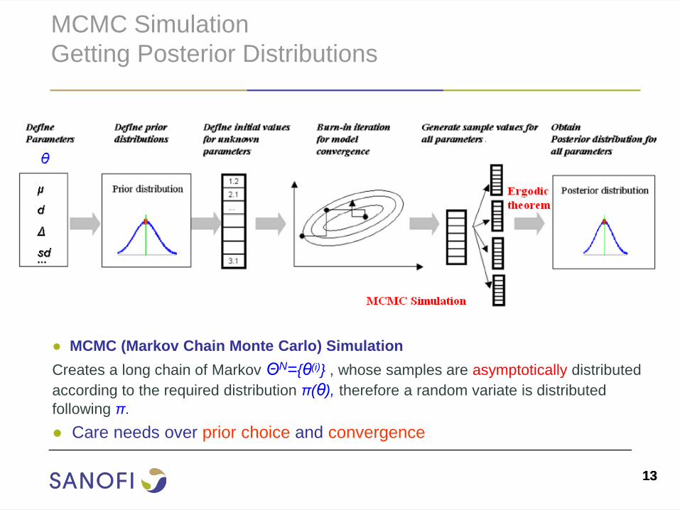
MCMC Simulation
Getting Posterior Distributions
● MCMC (Markov Chain Monte Carlo) Simulation
Creates a long chain of Markov ΘN={θ(i)} , whose samples are asymptotically distributed
according to the required distribution π(θ), therefore a random variate is distributed
following π.
● Care needs over prior choice and convergence
14 14
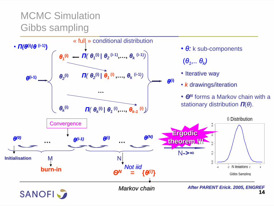
MCMC Simulation
Gibbs sampling
θ(i-1)
θ(i)
θ1(i) Π( θ1
(i) | θ2 (i-1),…, θk
(i-1))
θ2(i) Π( θ2
(i) | θ1 (i) ,…, θk
(i-1))
θk(i)
Π( θk(i) | θ1
(i),…, θk-1 (i) )
…
After PARENT Erick. 2005, ENGREF
M
burn-in
N
ΘN = {θ(i)}
… …
• θ: k sub-components
(θ1,.. θk)
• Iterative way
• k drawings/iteration
• ΘN forms a Markov chain with a
stationary distribution Π(θ).
-4 -2 0 2 4
0.0
0.1
0.2
0.3
0.4
Distribution
Gibbs Sampling
N iterations
Convergence
θ(i) θ(N) θ(i-1)
Ergodic
theorem !!! θ(0)
Initialisation
• Π(θ(i)/θ (i-1))
Not iid
N->∞
« full » conditional distribution
Markov chain
15 15
MCMC Simulation
Convergence diagnostics
1. Definition
● Convergence refers to the idea that MCMC technique will eventually
reach a stationary distribution.
(not a single value)
2. Main issus
1. How long for “burn-in”?
2. How many iterations after convergence?
• If the model has converged, further samples should not influence the
calculation of the mean
3. To identify non-convergence
● Simulate multi over-dispersed starting chains:
● Methods: plots and MC error
• Intuition: basically same behavior of all of the chains
16 16
Convergence Diagnostics
Plot diagnostics
1. Trajectory plot
• Plots: parameter value at time t vs. thinned iteration number
• Look like a snake around a stable mean value
2. Autocorrelation
• Autocorrelation refers to a pattern of serial correlation in the chain
• Thin the chains if high autocorrelation: storing every kth sample
3. Kernel density plots
• Same distribution of all chains
• Sometimes non-convergence is reflected in multimodal distributions.
=> let the algorithm run a bit longer
4. Gelman-Rubin (GR) Diagnostic
• Idea: Within-chain variance = Between-chain variance
17 17
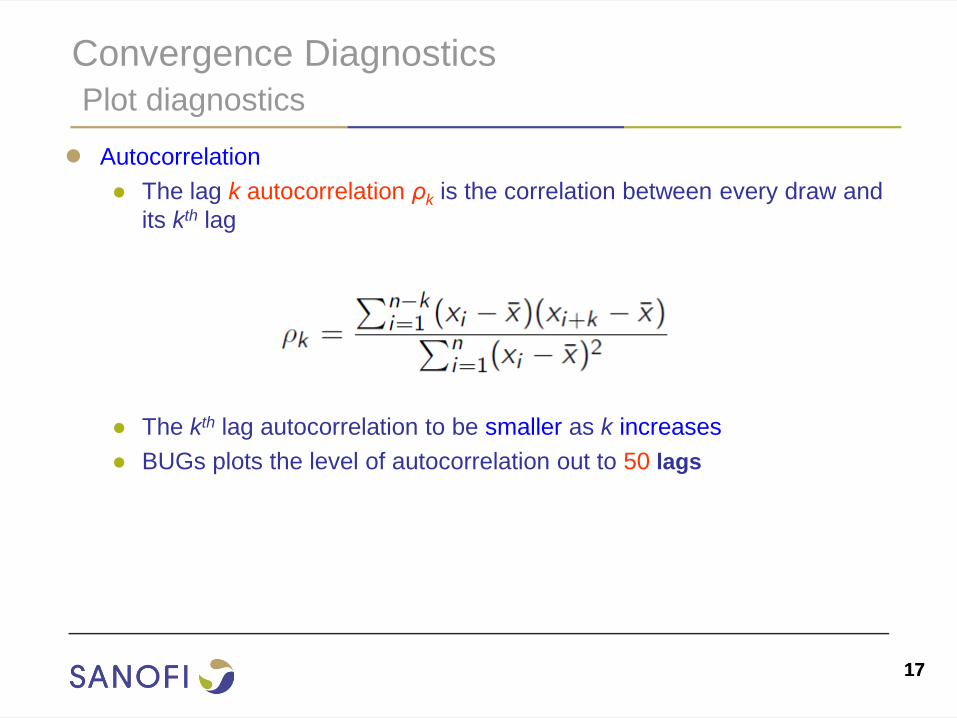
Convergence Diagnostics
Plot diagnostics
● Autocorrelation
● The lag k autocorrelation ρk is the correlation between every draw and
its kth lag
● The kth lag autocorrelation to be smaller as k increases
● BUGs plots the level of autocorrelation out to 50 lags
18 18
Convergence Diagnostics
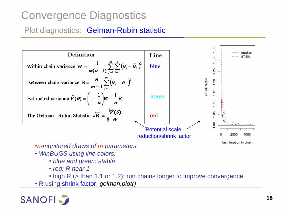
Plot diagnostics: Gelman-Rubin statistic
•n-monitored draws of m parameters
• WinBUGS using line colors:
• blue and green: stable
• red: R near 1
• high R (> than 1.1 or 1.2): run chains longer to improve convergence
• R using shrink factor: gelman.plot()
Potential scale
reduction/shrink factor
19 19
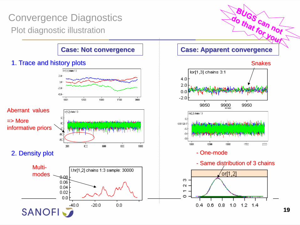
Convergence Diagnostics
Plot diagnostic illustration
1. Trace and history plots
Case: Not convergence
2. Density plot
Case: Apparent convergence
Aberrant values
=> More
informative priors
Snakes
Multi-
modes
- One-mode
- Same distribution of 3 chains
20 20
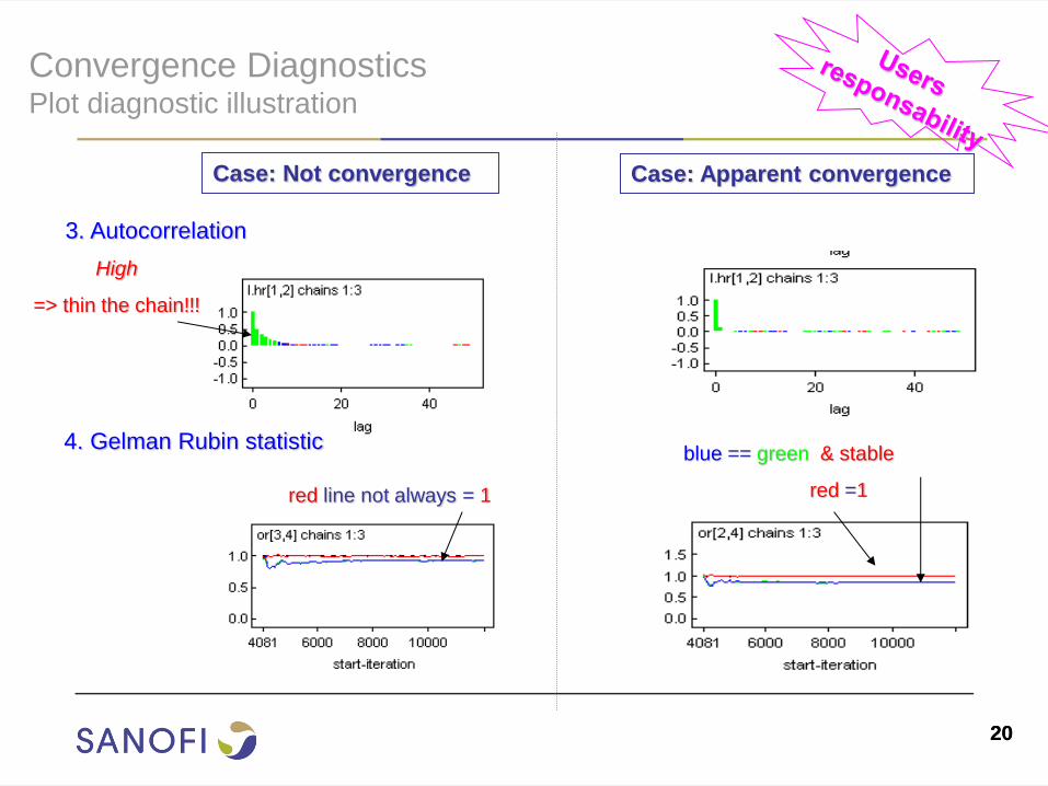
Convergence Diagnostics Plot diagnostic illustration
blue == green & stable
red =1
3. Autocorrelation
4. Gelman Rubin statistic
Case: Not convergence Case: Apparent convergence
High
=> thin the chain!!!
red line not always = 1
21 21
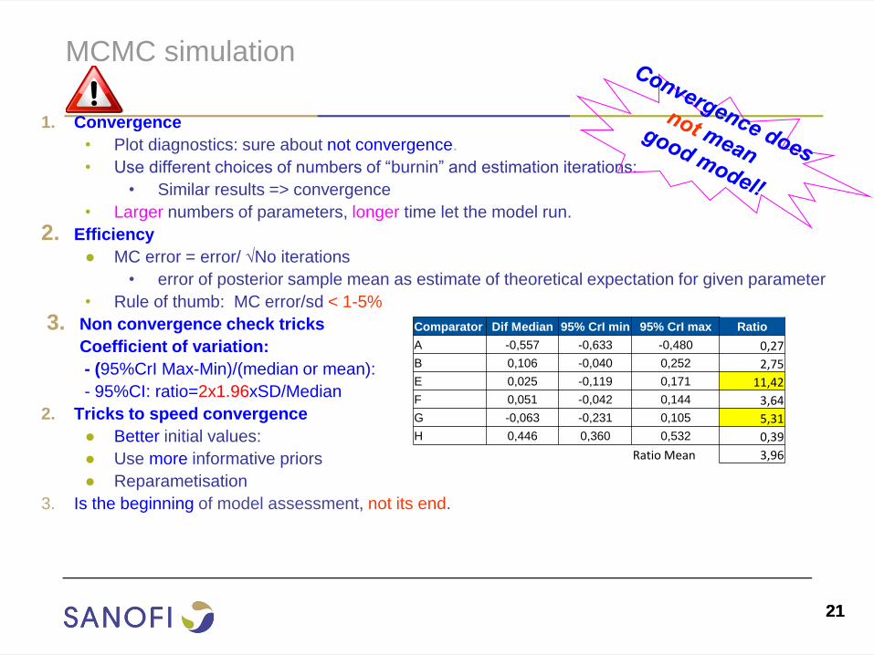
MCMC simulation
1. Convergence
• Plot diagnostics: sure about not convergence.
• Use different choices of numbers of “burnin” and estimation iterations:
• Similar results => convergence
• Larger numbers of parameters, longer time let the model run.
2. Efficiency
● MC error = error/ √No iterations
• error of posterior sample mean as estimate of theoretical expectation for given parameter
• Rule of thumb: MC error/sd < 1-5%
3. Non convergence check tricks
Coefficient of variation:
- (95%CrI Max-Min)/(median or mean):
- 95%CI: ratio=2x1.96xSD/Median
2. Tricks to speed convergence
● Better initial values:
● Use more informative priors
● Reparametisation
3. Is the beginning of model assessment, not its end.
Comparator Dif Median 95% CrI min 95% CrI max Ratio
A -0,557 -0,633 -0,480 0,27
B 0,106 -0,040 0,252 2,75
E 0,025 -0,119 0,171 11,42
F 0,051 -0,042 0,144 3,64
G -0,063 -0,231 0,105 5,31
H 0,446 0,360 0,532 0,39
Ratio Mean 3,96
II. NMA with Bayesian approach
A. Bayesian context
• Bayesian inference
• MCMC Simulation
• Convergence Diagnostic
B. Implementation
• NMA structure in BUGS
• Case of binary outcome
C. How to run BUGS?
22 22
23 23
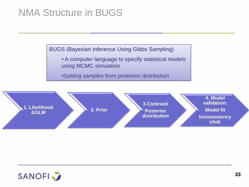
NMA Structure in BUGS
BUGS (Bayesian Inference Using Gibbs Sampling)
• A computer language to specify statistical models
using MCMC simulation
•Getting samples from posteriori distribution
1. Likelihood &GLM
2. Prior
3.Contrast/
Posterior distribution
4. Model validation:
Model fit
Inconsistency chek
24 24
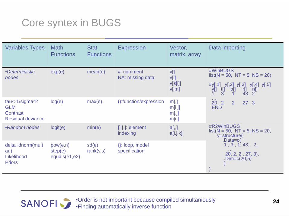
Core syntex in BUGS
Variables Types Math
Functions
Stat
Functions
Expression Vector,
matrix, array
Data importing
•Deterministic
nodes
exp(e) mean(e) #: comment
NA: missing data
v[]
v[i]
v[s[i]]
v[i:n]
#WinBUGS list(N = 50, NT = 5, NS = 20) #y[,1] y[,2] y[,3] y[,4] y[,5] y[] t[] b[] r[] n[] 1 3 1 43 2 … 20 2 2 27 3 END
tau<-1/sigma^2
GLM
Contrast
Residual deviance
log(e) max(e) ():function/expression
m[,]
m[i,j]
m[,j]
m[i,]
•Random nodes logit(e)
min(e)
[] [,]: element
indexing
a[,,]
a[i,j,k]
#R2WinBUGS list(N = 50, NT = 5, NS = 20, y=structure( .Data=c( 1 , 3 , 1, 43, 2, … 20, 2, 2 , 27, 3), .Dim=c(20,5) )
)
delta~dnorm(mu,t
au)
Likelihood
Priors
pow(e,n)
step(e)
equals(e1,e2)
sd(e)
rank(v,s)
{}: loop, model
specification
•Order is not important because compiled simultaniously
•Finding automatically inverse function
25 25
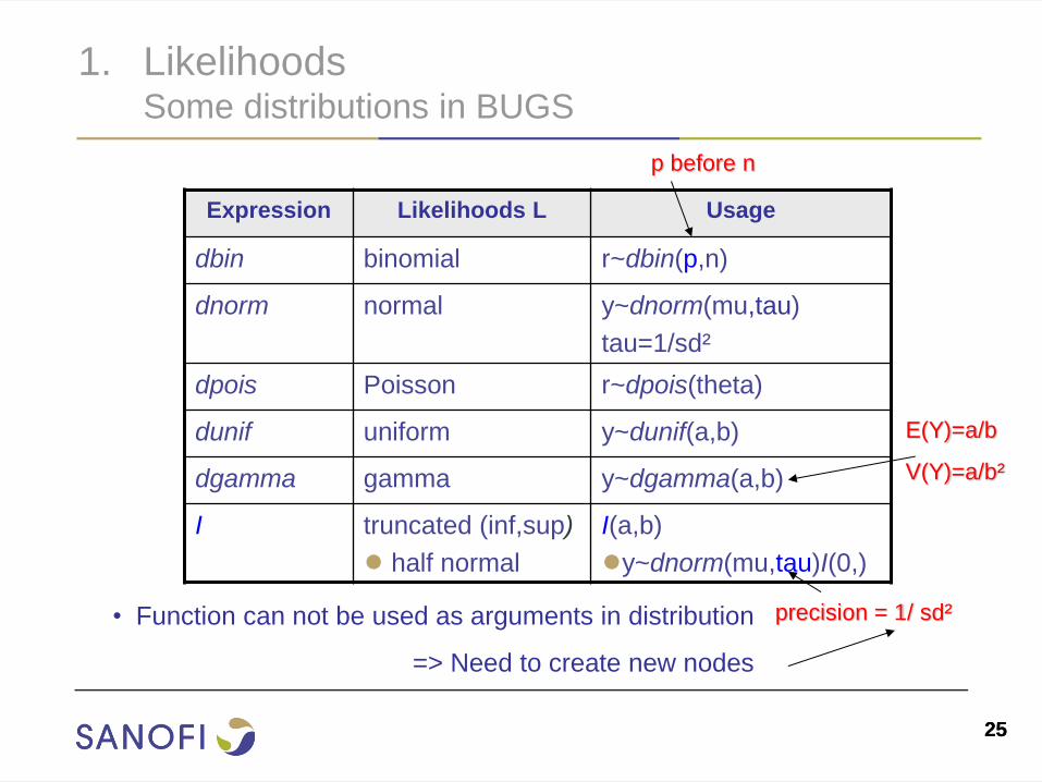
1. Likelihoods Some distributions in BUGS
Expression Likelihoods L Usage
dbin binomial r~dbin(p,n)
dnorm normal y~dnorm(mu,tau)
tau=1/sd²
dpois Poisson r~dpois(theta)
dunif uniform y~dunif(a,b)
dgamma gamma y~dgamma(a,b)
I truncated (inf,sup)
● half normal
I(a,b)
●y~dnorm(mu,tau)I(0,)
precision = 1/ sd²
p before n
E(Y)=a/b
V(Y)=a/b²
• Function can not be used as arguments in distribution
=> Need to create new nodes
28 28
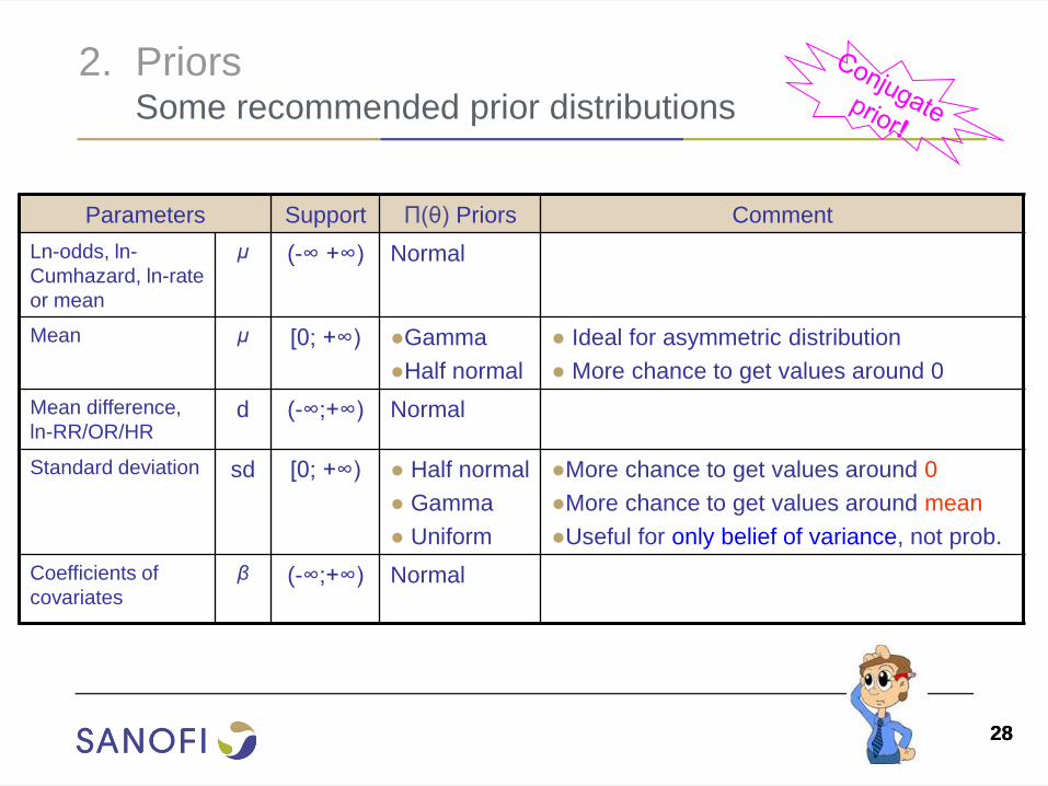
2. Priors Some recommended prior distributions
Parameters Support Π(θ) Priors Comment
Ln-odds, ln-
Cumhazard, ln-rate
or mean
μ
(-∞ +∞) Normal
Mean
μ [0; +∞) ●Gamma
●Half normal
● Ideal for asymmetric distribution
● More chance to get values around 0
Mean difference,
ln-RR/OR/HR d (-∞;+∞) Normal
Standard deviation sd [0; +∞) ● Half normal
● Gamma
● Uniform
●More chance to get values around 0
●More chance to get values around mean
●Useful for only belief of variance, not prob.
Coefficients of
covariates
β
(-∞;+∞) Normal
29 29
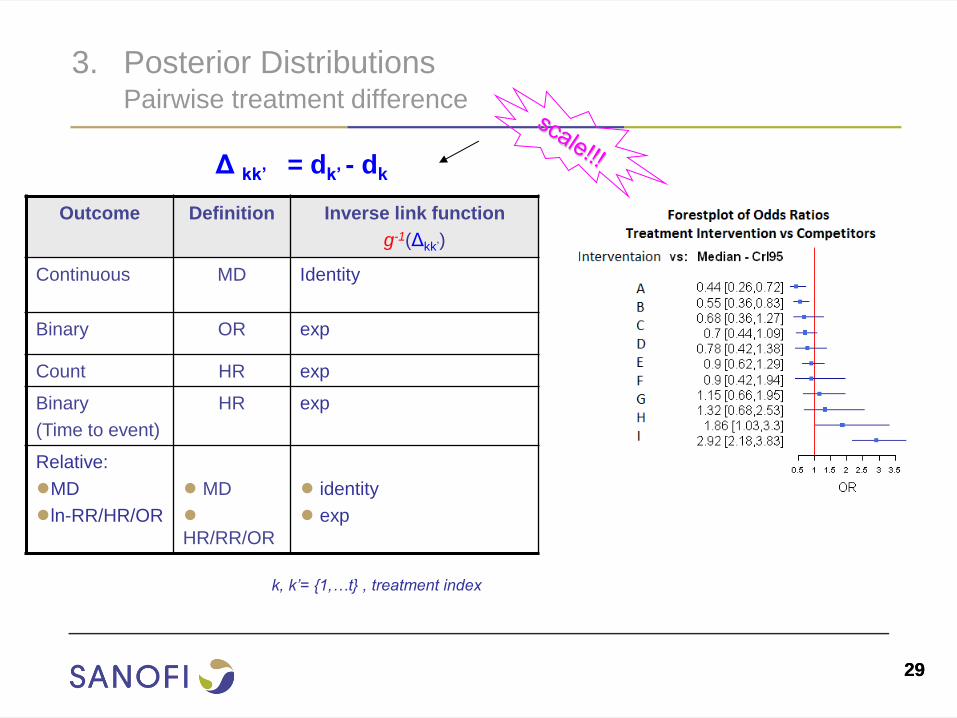
3. Posterior Distributions Pairwise treatment difference
Outcome
Definition Inverse link function
g-1(Δkk’)
Continuous MD Identity
Binary OR exp
Count HR exp
Binary
(Time to event)
HR exp
Relative:
●MD
●ln-RR/HR/OR
● MD
●
HR/RR/OR
● identity
● exp
Δ kk’ = dk’ - dk
k, k’= {1,…t} , treatment index
30 30
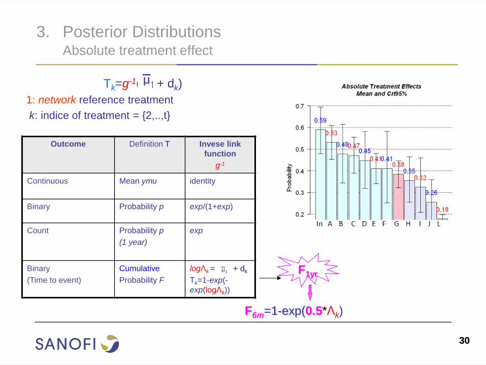
3. Posterior Distributions Absolute treatment effect
Outcome Definition T Invese link
function
g-1
Continuous Mean ymu identity
Binary Probability p exp/(1+exp)
Count Probability p
(1 year)
exp
Binary
(Time to event)
Cumulative
Probability F
logΛk = + dk
Tk=1-exp(-
exp(logΛk))
Tk=g-1( + dk)
1: network reference treatment
k: indice of treatment = {2,..,t}
F1yr
F6m=1-exp(0.5*Λk)
31 31
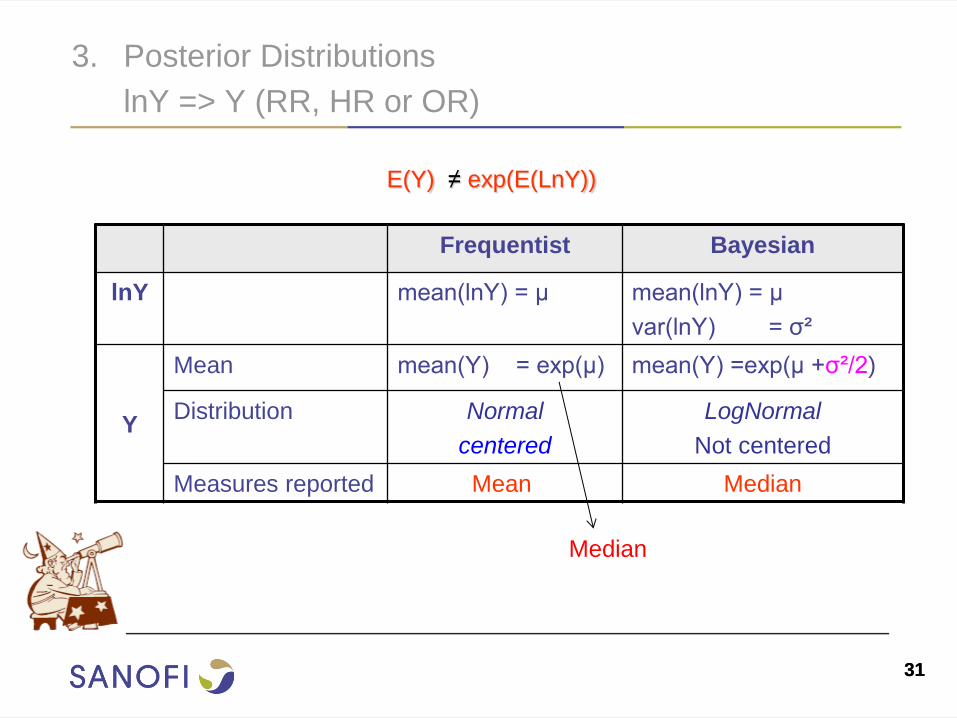
3. Posterior Distributions lnY => Y (RR, HR or OR)
Frequentist Bayesian
lnY mean(lnY) = μ
mean(lnY) = μ
var(lnY) = σ²
Y
Mean mean(Y) = exp(μ) mean(Y) =exp(μ +σ²/2)
Distribution Normal
centered
LogNormal
Not centered
Measures reported Mean Median
E(Y) ≠ exp(E(LnY))
Median
32 32
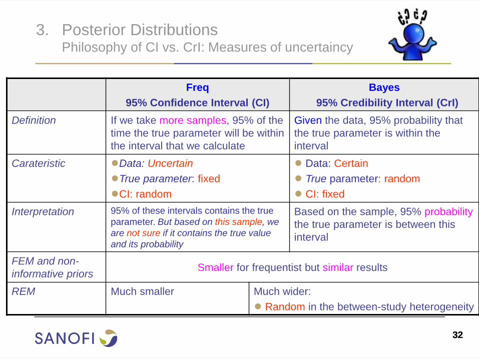
3. Posterior Distributions Philosophy of CI vs. CrI: Measures of uncertaincy
Freq
95% Confidence Interval (CI)
Bayes
95% Credibility Interval (CrI)
Definition If we take more samples, 95% of the
time the true parameter will be within
the interval that we calculate
Given the data, 95% probability that
the true parameter is within the
interval
Carateristic ●Data: Uncertain
●True parameter: fixed
●CI: random
● Data: Certain
● True parameter: random
● CI: fixed
Interpretation 95% of these intervals contains the true
parameter. But based on this sample, we
are not sure if it contains the true value
and its probability
Based on the sample, 95% probability
the true parameter is between this
interval
FEM and non-
informative priors Smaller for frequentist but similar results
REM Much smaller Much wider:
● Random in the between-study heterogeneity
33 33
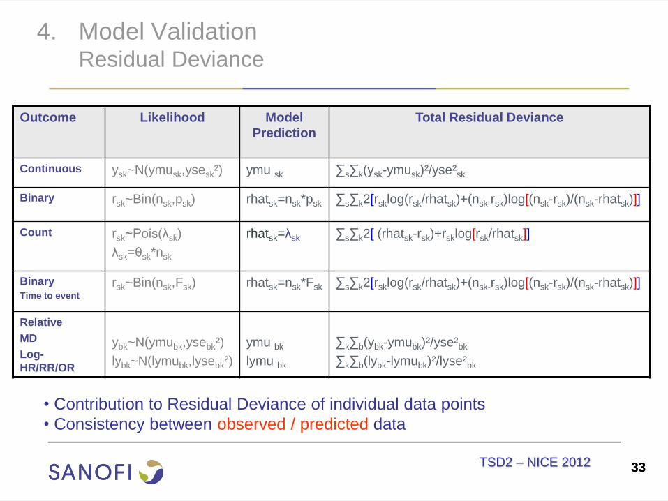
4. Model Validation Residual Deviance
Outcome Likelihood Model
Prediction
Total Residual Deviance
Continuous ysk~N(ymusk,ysesk²) ymu sk ∑s∑k(ysk-ymusk)²/yse²sk
Binary rsk~Bin(nsk,psk) rhatsk=nsk*psk ∑s∑k2[rsklog(rsk/rhatsk)+(nsk-rsk)log[(nsk-rsk)/(nsk-rhatsk)]]
Count
rsk~Pois(λsk)
λsk=θsk*nsk
rhatsk=λsk ∑s∑k2[ (rhatsk-rsk)+rsklog[rsk/rhatsk]]
Binary
Time to event
rsk~Bin(nsk,Fsk) rhatsk=nsk*Fsk
∑s∑k2[rsklog(rsk/rhatsk)+(nsk-rsk)log[(nsk-rsk)/(nsk-rhatsk)]]
Relative
MD
Log-
HR/RR/OR
ybk~N(ymubk,ysebk²)
lybk~N(lymubk,lysebk²)
ymu bk
lymu bk
∑k∑b(ybk-ymubk)²/yse²bk
∑k∑b(lybk-lymubk)²/lyse²bk
• Contribution to Residual Deviance of individual data points
• Consistency between observed / predicted data
TSD2 – NICE 2012
34 34
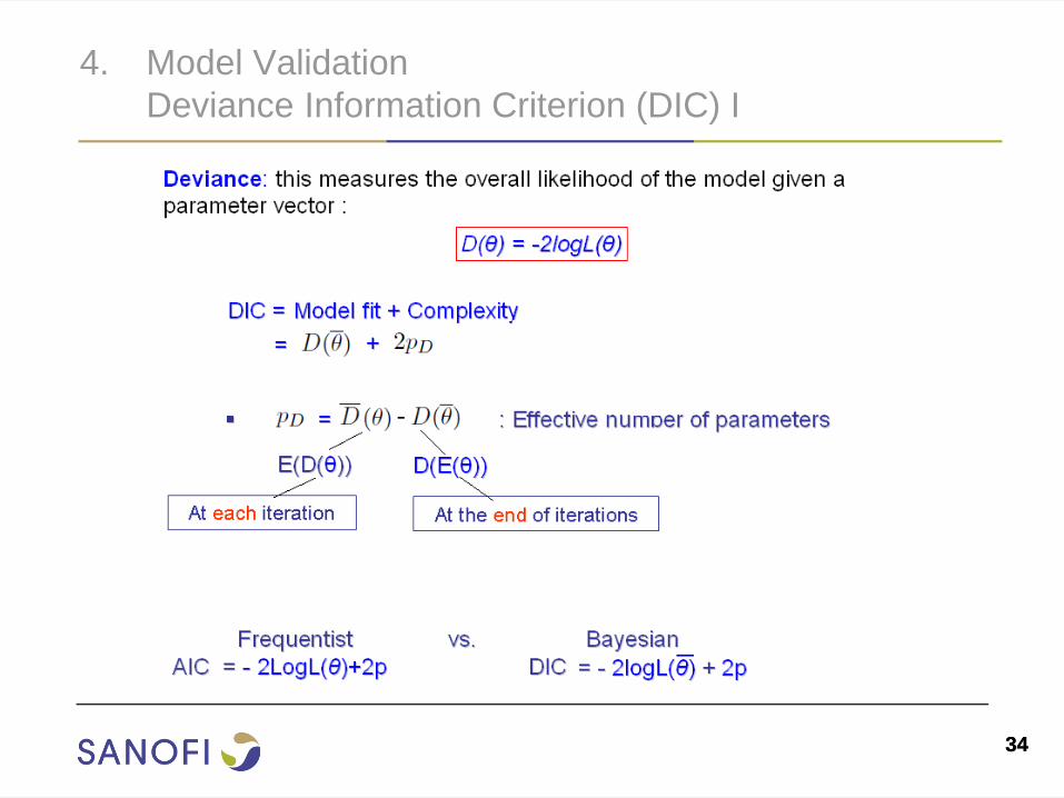
4. Model Validation
Deviance Information Criterion (DIC) I
35
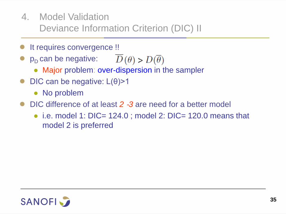
● It requires convergence !!
● pD can be negative:
● Major problem: over‐dispersion in the sampler
● DIC can be negative: L(θ)>1
● No problem
● DIC difference of at least 2 ‐3 are need for a better model
● i.e. model 1: DIC= 124.0 ; model 2: DIC= 120.0 means that
model 2 is preferred
4. Model Validation
Deviance Information Criterion (DIC) II
36 36
4. Model Validation
Tool for goodness of fit
1. Residual deviance:
• Total residual deviance
• ~ N (number of arms )
• Mean residual deviance by arm: (total RD divided by N)
• ~ 1
• Useful for comparing models with different number of arms
2. DIC
Lower DIC suggests a more parsimonious model
• Useful for comparing different parameter models
• eg.: FEM vs REM or models with and without covariates
3. Comparing NMA and direct results
Model with results most similar to direct results (mean/median, CrI vs CI)
37 37
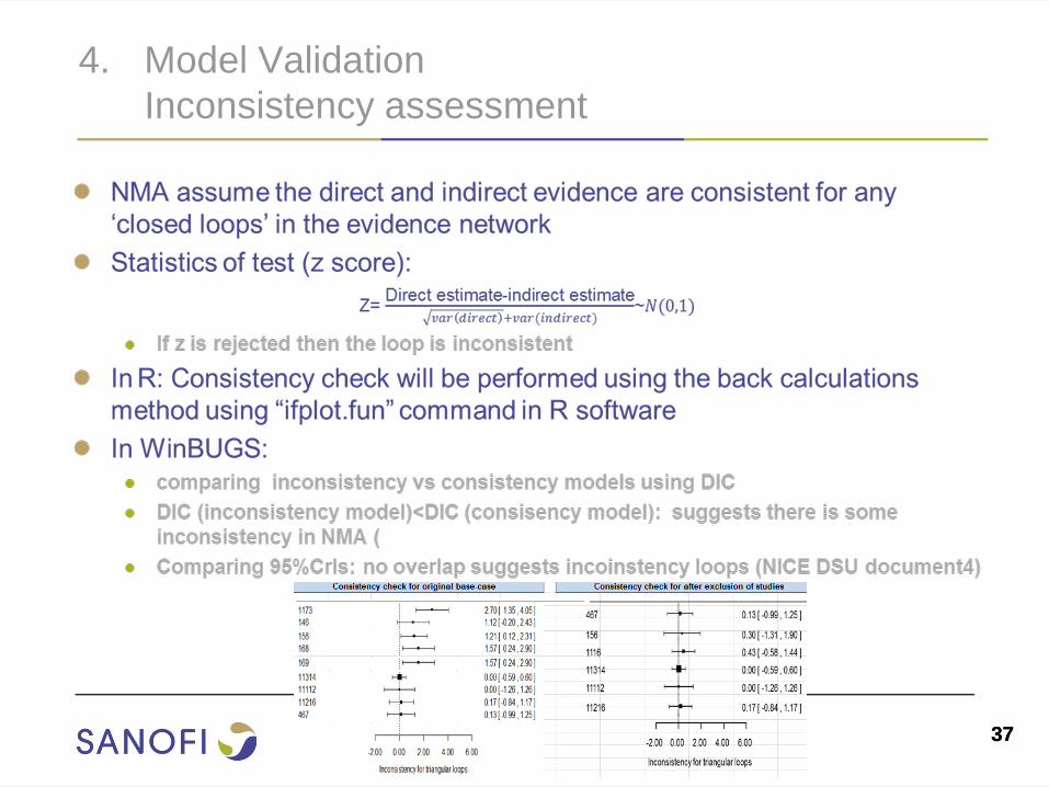
4. Model Validation
Inconsistency assessment

38 38
4. Model Validation
Sensitivity analysis
1. Prior choice
● In REM:
• Between-study variance/sd is poorly estimated due to few data
=> Importance of priors for between-study sd
• Using DIC
2. After deleting some studies (if necessary)
• Using mean residual deviance by arm
3. NMA with covariate
• Using DIC et mean residual deviance by arm
39 39
Case of binary outcome
● BUGS Data Format
● BUGS Code
• FEM
• REM
40 40
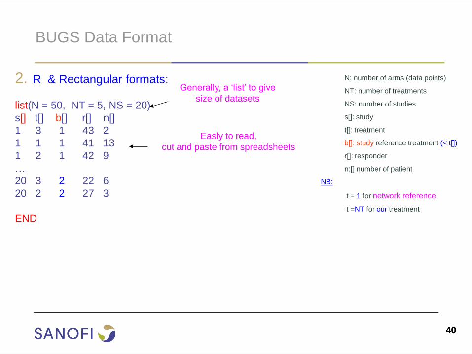
BUGS Data Format
2. R & Rectangular formats:
list(N = 50, NT = 5, NS = 20)
s[] t[] b[] r[] n[]
1 3 1 43 2
1 1 1 41 13
1 2 1 42 9
…
20 3 2 22 6
20 2 2 27 3
END
N: number of arms (data points)
NT: number of treatments
NS: number of studies
s[]: study
t[]: treatment
b[]: study reference treatment (< t[])
r[]: responder
n:[] number of patient
NB:
t = 1 for network reference
t =NT for our treatment
Generally, a ‘list’ to give
size of datasets
Easly to read,
cut and paste from spreadsheets
41 41
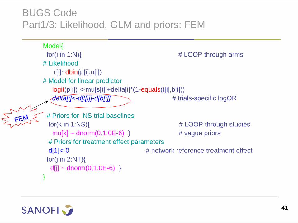
BUGS Code
Part1/3: Likelihood, GLM and priors: FEM
Model{
for(i in 1:N){ # LOOP through arms
# Likelihood
r[i]~dbin(p[i],n[i])
# Model for linear predictor
logit(p[i]) <-mu[s[i]]+delta[i]*(1-equals(t[i],b[i]))
delta[i]<-d[t[i]]-d[b[i]] # trials-specific logOR
# Priors for NS trial baselines
for(k in 1:NS){ # LOOP through studies
mu[k] ~ dnorm(0,1.0E-6) } # vague priors
# Priors for treatment effect parameters
d[1]<-0 # network reference treatment effect
for(j in 2:NT){
d[j] ~ dnorm(0,1.0E-6) }
}
42 42
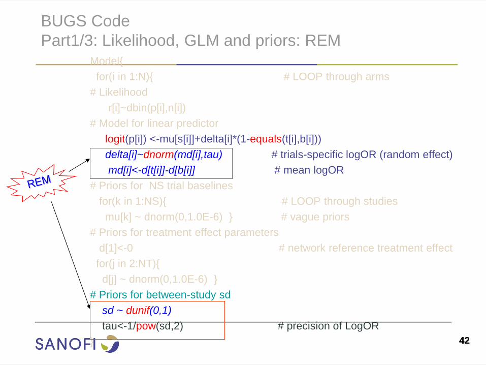
BUGS Code
Part1/3: Likelihood, GLM and priors: REM Model{
for(i in 1:N){ # LOOP through arms
# Likelihood
r[i]~dbin(p[i],n[i])
# Model for linear predictor
logit(p[i]) <-mu[s[i]]+delta[i]*(1-equals(t[i],b[i]))
delta[i]~dnorm(md[i],tau) # trials-specific logOR (random effect)
md[i]<-d[t[i]]-d[b[i]] # mean logOR
# Priors for NS trial baselines
for(k in 1:NS){ # LOOP through studies
mu[k] ~ dnorm(0,1.0E-6) } # vague priors
# Priors for treatment effect parameters
d[1]<-0 # network reference treatment effect
for(j in 2:NT){
d[j] ~ dnorm(0,1.0E-6) }
# Priors for between-study sd
sd ~ dunif(0,1)
tau<-1/pow(sd,2) # precision of LogOR
}
43 43
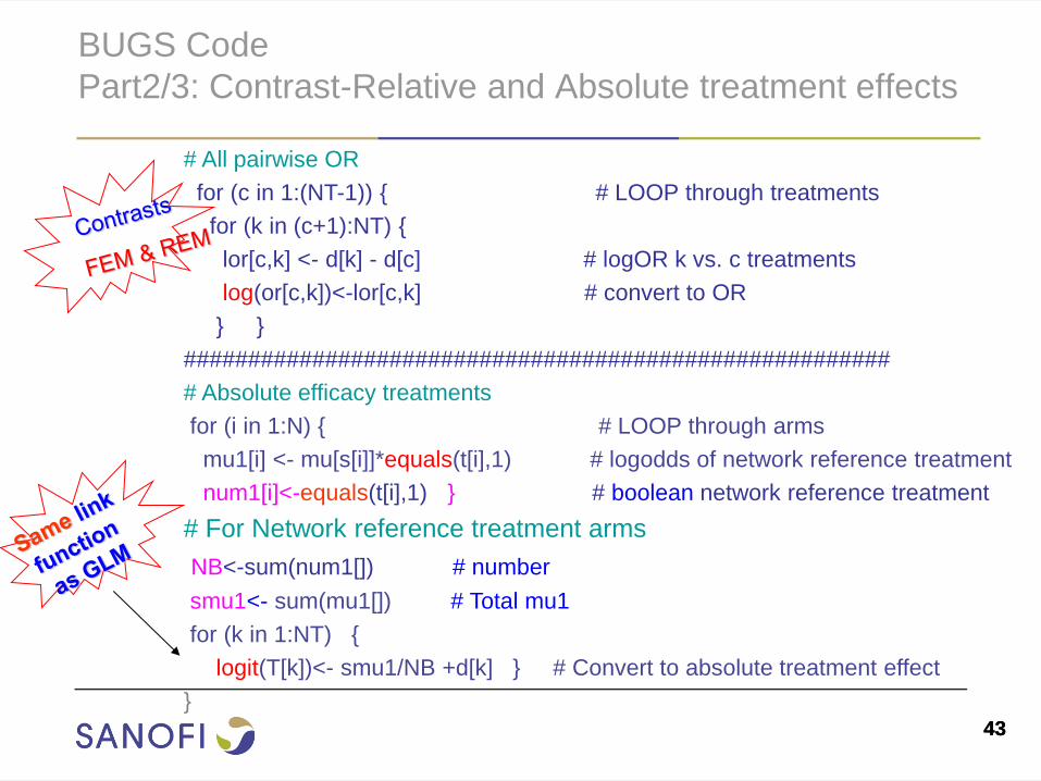
BUGS Code
Part2/3: Contrast-Relative and Absolute treatment effects
# All pairwise OR
for (c in 1:(NT-1)) { # LOOP through treatments
for (k in (c+1):NT) {
lor[c,k] <- d[k] - d[c] # logOR k vs. c treatments
log(or[c,k])<-lor[c,k] # convert to OR
} }
#######################################################
# Absolute efficacy treatments
for (i in 1:N) { # LOOP through arms
mu1[i] <- mu[s[i]]*equals(t[i],1) # logodds of network reference treatment
num1[i]<-equals(t[i],1) } # boolean network reference treatment
# For Network reference treatment arms
NB<-sum(num1[]) # number
smu1<- sum(mu1[]) # Total mu1
for (k in 1:NT) {
logit(T[k])<- smu1/NB +d[k] } # Convert to absolute treatment effect
}
44 44
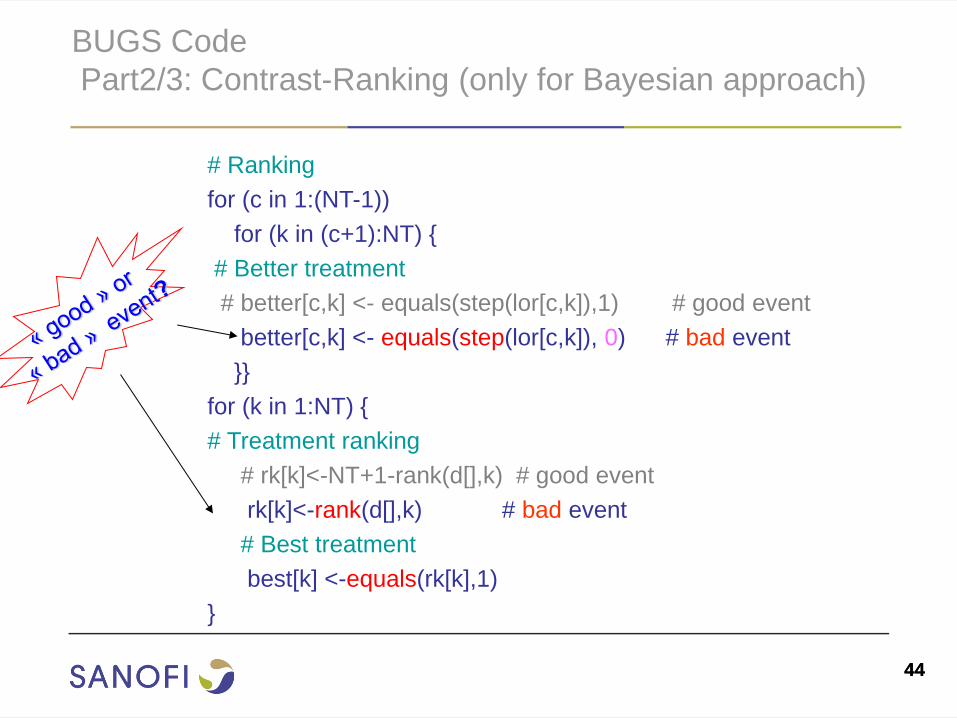
BUGS Code
Part2/3: Contrast-Ranking (only for Bayesian approach)
# Ranking
for (c in 1:(NT-1))
for (k in (c+1):NT) {
# Better treatment
# better[c,k] <- equals(step(lor[c,k]),1) # good event
better[c,k] <- equals(step(lor[c,k]), 0) # bad event
}}
for (k in 1:NT) {
# Treatment ranking
# rk[k]<-NT+1-rank(d[],k) # good event
rk[k]<-rank(d[],k) # bad event
# Best treatment
best[k] <-equals(rk[k],1)
}
45 45
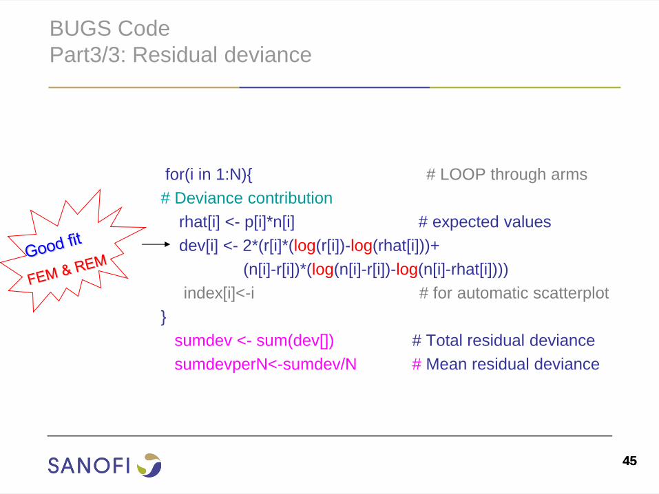
BUGS Code
Part3/3: Residual deviance
for(i in 1:N){ # LOOP through arms
# Deviance contribution
rhat[i] <- p[i]*n[i] # expected values
dev[i] <- 2*(r[i]*(log(r[i])-log(rhat[i]))+
(n[i]-r[i])*(log(n[i]-r[i])-log(n[i]-rhat[i])))
index[i]<-i # for automatic scatterplot
}
sumdev <- sum(dev[]) # Total residual deviance
sumdevperN<-sumdev/N # Mean residual deviance
II. NMA with Bayesian approach
A. Bayesian context
• Bayesian inference
• MCMC Simulation
• Convergence Diagnostic
B. Implementation
• NMA structure in BUGS
• Case of binary outcome
C. How to run BUGS?
• By hand
• By script
• By R
46 46
47 47
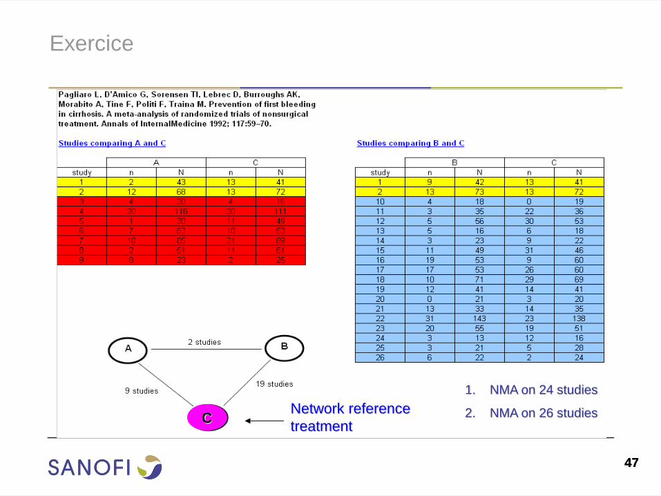
Exercice
C Network reference
treatment
1. NMA on 24 studies
2. NMA on 26 studies
49 49
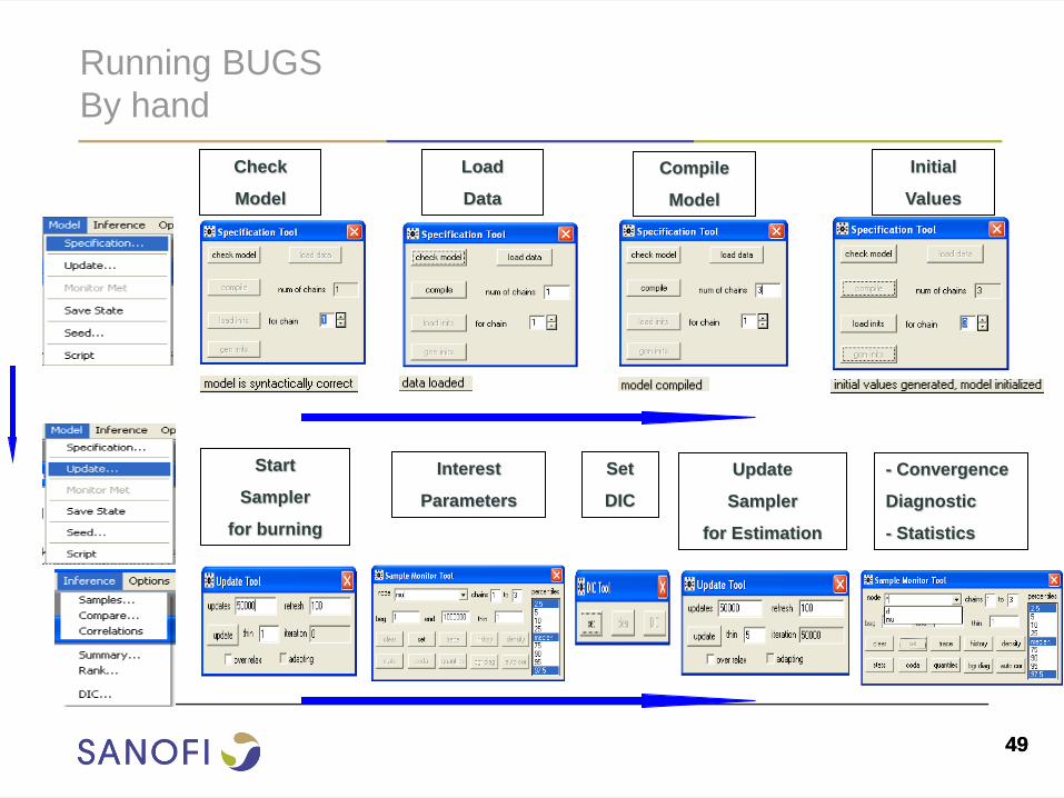
Running BUGS
By hand
Check
Model
Load
Data
Compile
Model
Initial
Values
Start
Sampler
for burning
Update
Sampler
for Estimation
Interest
Parameters
- Convergence
Diagnostic
- Statistics
Set
DIC
51 51
Initial values
● BUGS can automatically generate initial values for the MCMC analysis
using gen inits
● Fine if have informative priors
● Better to provide reasonable values in an initial values in case of non
informative priors
● Can be after model description or in a separate file.
● Same format as inputs
52 52
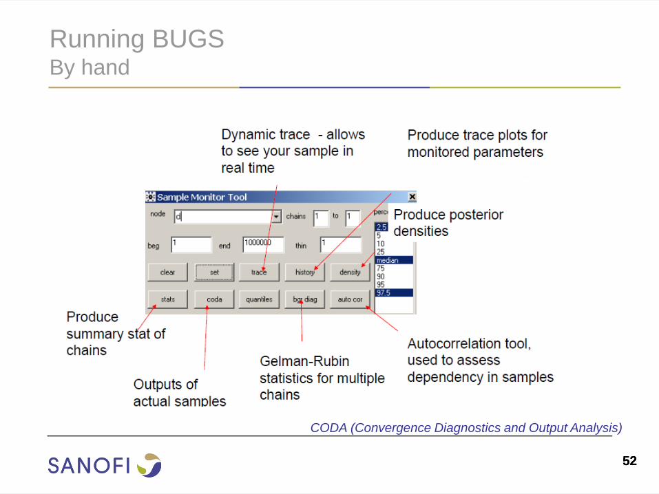
Running BUGS By hand
CODA (Convergence Diagnostics and Output Analysis)
53 53
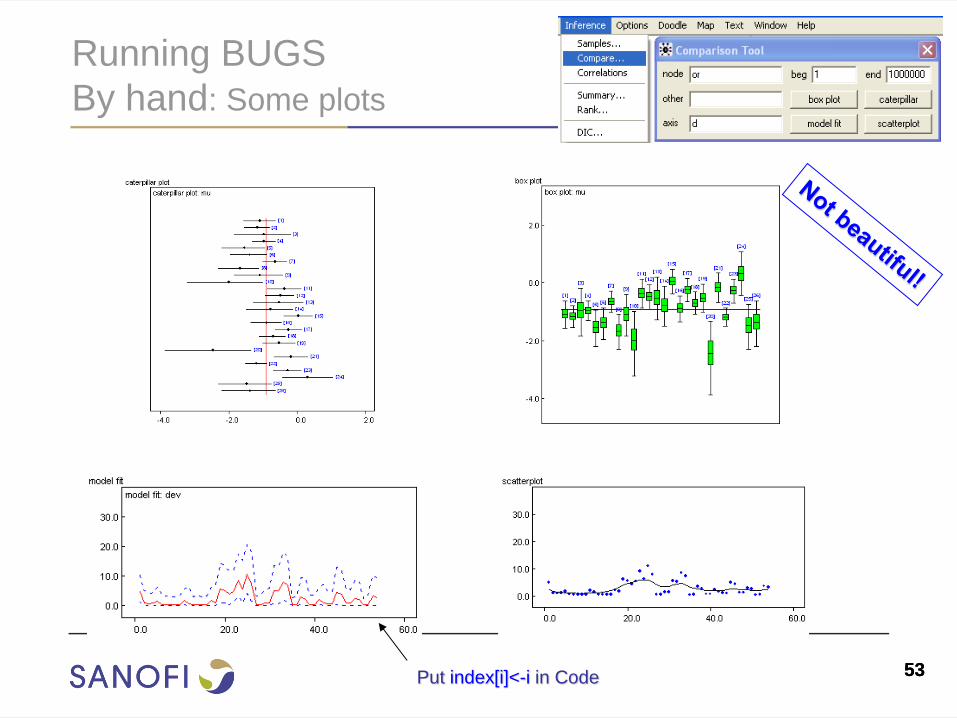
Running BUGS
By hand: Some plots
Put index[i]<-i in Code
54 54
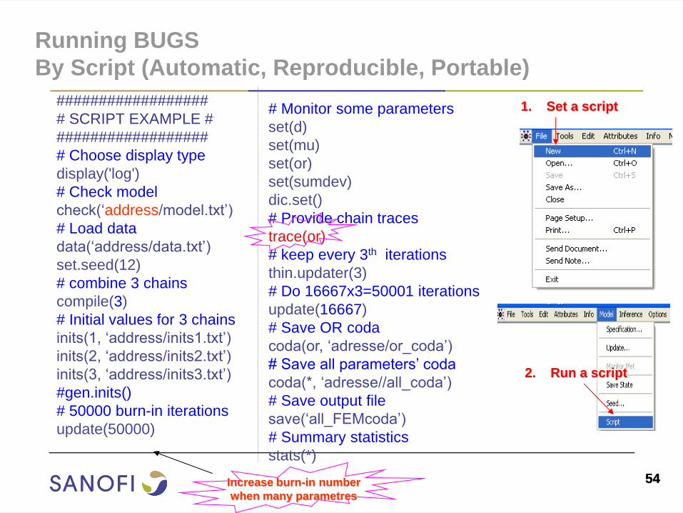
Running BUGS
By Script (Automatic, Reproducible, Portable)
##################
# SCRIPT EXAMPLE #
##################
# Choose display type
display('log')
# Check model
check(‘address/model.txt’)
# Load data
data(‘address/data.txt’)
set.seed(12)
# combine 3 chains
compile(3)
# Initial values for 3 chains
inits(1, ‘address/inits1.txt’)
inits(2, ‘address/inits2.txt’)
inits(3, ‘address/inits3.txt’)
#gen.inits()
# 50000 burn-in iterations
update(50000)
# Monitor some parameters
set(d)
set(mu)
set(or)
set(sumdev)
dic.set()
# Provide chain traces
trace(or)
# keep every 3th iterations
thin.updater(3)
# Do 16667x3=50001 iterations
update(16667)
# Save OR coda
coda(or, ‘adresse/or_coda’)
# Save all parameters’ coda
coda(*, ‘adresse//all_coda’)
# Save output file
save(‘all_FEMcoda’)
# Summary statistics
stats(*)
1. Set a script
2. Run a script
Increase burn-in number
when many parametres
55 55
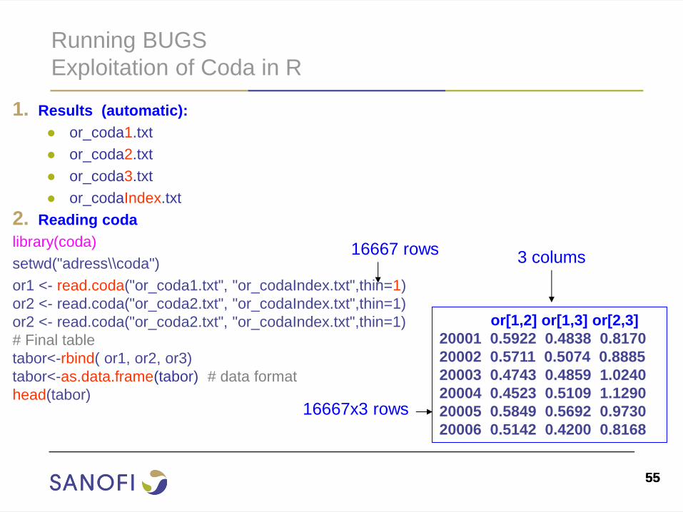
Running BUGS
Exploitation of Coda in R
1. Results (automatic):
● or_coda1.txt
● or_coda2.txt
● or_coda3.txt
● or_codaIndex.txt
2. Reading coda
library(coda)
setwd("adress\\coda")
or1 <- read.coda("or_coda1.txt", "or_codaIndex.txt",thin=1)
or2 <- read.coda("or_coda2.txt", "or_codaIndex.txt",thin=1)
or2 <- read.coda("or_coda2.txt", "or_codaIndex.txt",thin=1)
# Final table
tabor<-rbind( or1, or2, or3)
tabor<-as.data.frame(tabor) # data format
head(tabor)
16667 rows 3 colums
or[1,2] or[1,3] or[2,3]
20001 0.5922 0.4838 0.8170
20002 0.5711 0.5074 0.8885
20003 0.4743 0.4859 1.0240
20004 0.4523 0.5109 1.1290
20005 0.5849 0.5692 0.9730
20006 0.5142 0.4200 0.8168
16667x3 rows
58 58
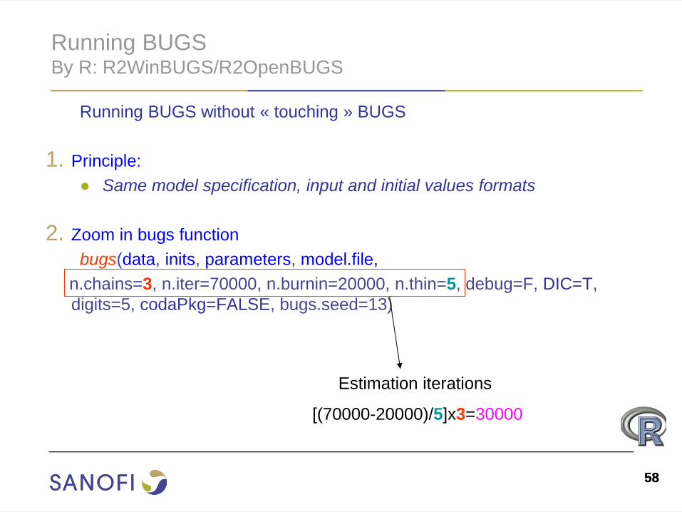
Running BUGS By R: R2WinBUGS/R2OpenBUGS
Running BUGS without « touching » BUGS
1. Principle:
● Same model specification, input and initial values formats
2. Zoom in bugs function
bugs(data, inits, parameters, model.file,
n.chains=3, n.iter=70000, n.burnin=20000, n.thin=5, debug=F, DIC=T,
digits=5, codaPkg=FALSE, bugs.seed=13)
Estimation iterations
[(70000-20000)/5]x3=30000
59 59
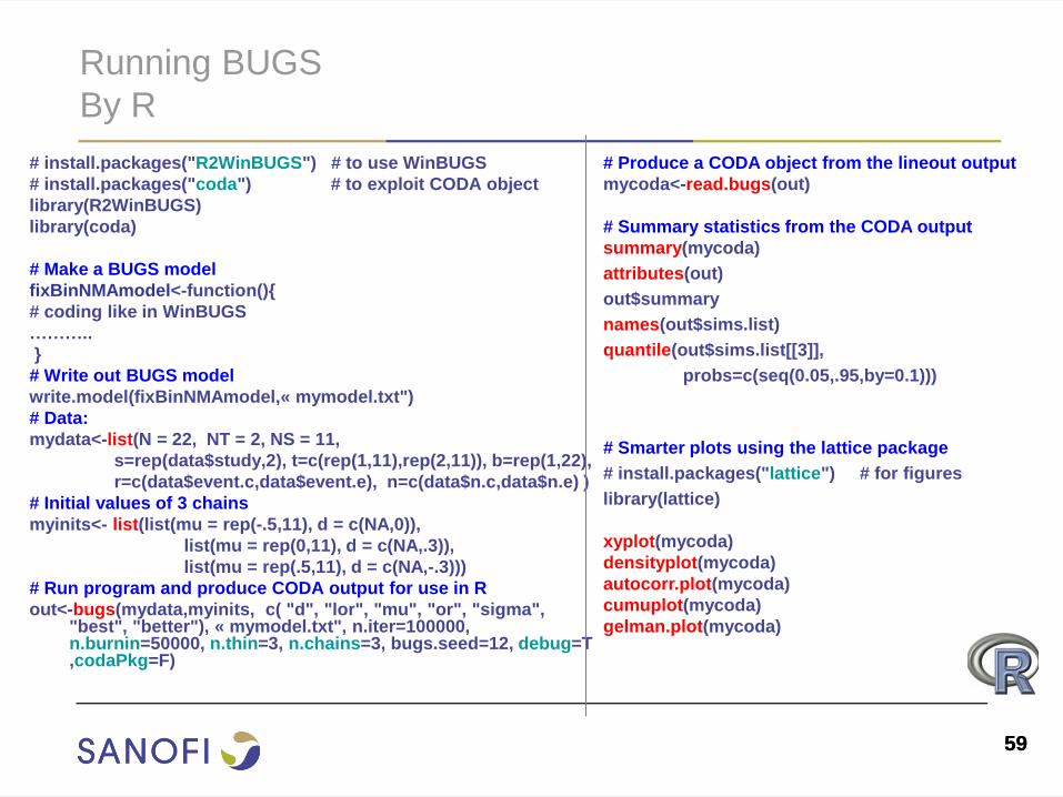
Running BUGS
By R
# install.packages("R2WinBUGS") # to use WinBUGS
# install.packages("coda") # to exploit CODA object
library(R2WinBUGS)
library(coda)
# Make a BUGS model
fixBinNMAmodel<-function(){
# coding like in WinBUGS
………..
}
# Write out BUGS model
write.model(fixBinNMAmodel,« mymodel.txt")
# Data:
mydata<-list(N = 22, NT = 2, NS = 11,
s=rep(data$study,2), t=c(rep(1,11),rep(2,11)), b=rep(1,22),
r=c(data$event.c,data$event.e), n=c(data$n.c,data$n.e) )
# Initial values of 3 chains
myinits<- list(list(mu = rep(-.5,11), d = c(NA,0)),
list(mu = rep(0,11), d = c(NA,.3)),
list(mu = rep(.5,11), d = c(NA,-.3)))
# Run program and produce CODA output for use in R
out<-bugs(mydata,myinits, c( "d", "lor", "mu", "or", "sigma", "best", "better"), « mymodel.txt", n.iter=100000, n.burnin=50000, n.thin=3, n.chains=3, bugs.seed=12, debug=T ,codaPkg=F)
# Produce a CODA object from the lineout output
mycoda<-read.bugs(out)
# Summary statistics from the CODA output
summary(mycoda)
attributes(out)
out$summary
names(out$sims.list)
quantile(out$sims.list[[3]],
probs=c(seq(0.05,.95,by=0.1)))
# Smarter plots using the lattice package
# install.packages("lattice") # for figures
library(lattice)
xyplot(mycoda)
densityplot(mycoda)
autocorr.plot(mycoda)
cumuplot(mycoda)
gelman.plot(mycoda)
60
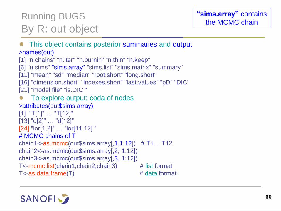
Running BUGS
By R: out object
● This object contains posterior summaries and output >names(out)
[1] "n.chains" "n.iter" "n.burnin" "n.thin" "n.keep"
[6] "n.sims" "sims.array" "sims.list" "sims.matrix" "summary"
[11] "mean" "sd" "median" "root.short" "long.short"
[16] "dimension.short" "indexes.short" "last.values" "pD" "DIC"
[21] "model.file" "is.DIC "
● To explore output: coda of nodes >attributes(out$sims.array)
[1] "T[1]" … "T[12]"
[13] "d[2]" … "d[12]"
[24] "lor[1,2]" … "lor[11,12] "
# MCMC chains of T
chain1<-as.mcmc(out$sims.array[,1,1:12]) # T1… T12
chain2<-as.mcmc(out$sims.array[,2, 1:12])
chain3<-as.mcmc(out$sims.array[,3, 1:12])
T<-mcmc.list(chain1,chain2,chain3) # list format
T<-as.data.frame(T) # data format
“sims.array” contains
the MCMC chain

61 61
IV. Practice
Binary outcome NMA
1. Exercice:
● Data
● Output interpretation
62 62
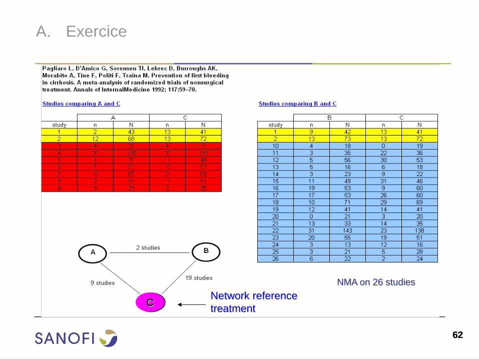
A. Exercice
C Network reference
treatment
NMA on 26 studies
63 63
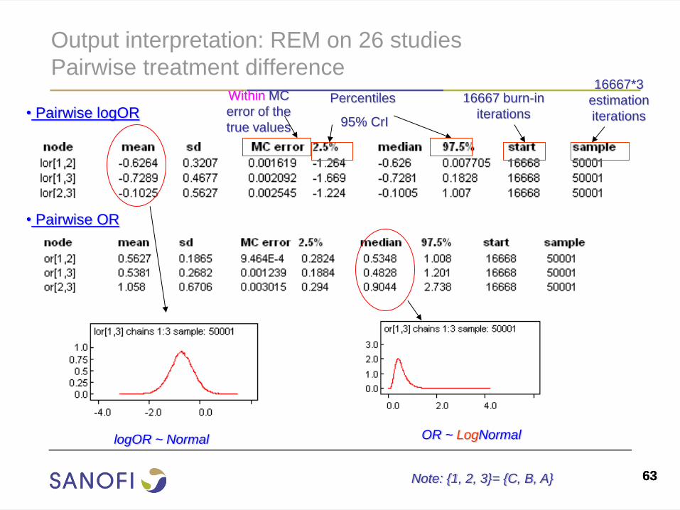
Output interpretation: REM on 26 studies
Pairwise treatment difference
logOR ~ Normal
• Pairwise logOR
• Pairwise OR
OR ~ LogNormal
Note: {1, 2, 3}= {C, B, A}
16667 burn-in
iterations
16667*3
estimation
iterations
Percentiles
95% CrI
Within MC
error of the
true values
64 64
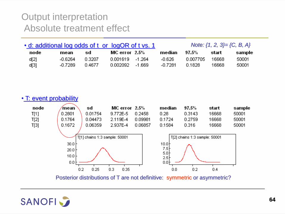
Output interpretation
Absolute treatment effect
• T: event probability
• d: additional log odds of t or logOR of t vs. 1
Posterior distributions of T are not definitive: symmetric or asymmetric?
Note: {1, 2, 3}= {C, B, A}
65 65
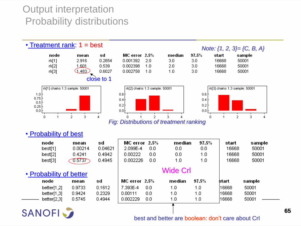
Output interpretation
Probability distributions
• Probability of better
• Treatment rank: 1 = best
• Probability of best
close to 1
Fig: Distributions of treatment ranking
best and better are boolean: don’t care about CrI
Note: {1, 2, 3}= {C, B, A}
Wide Crl
66 66
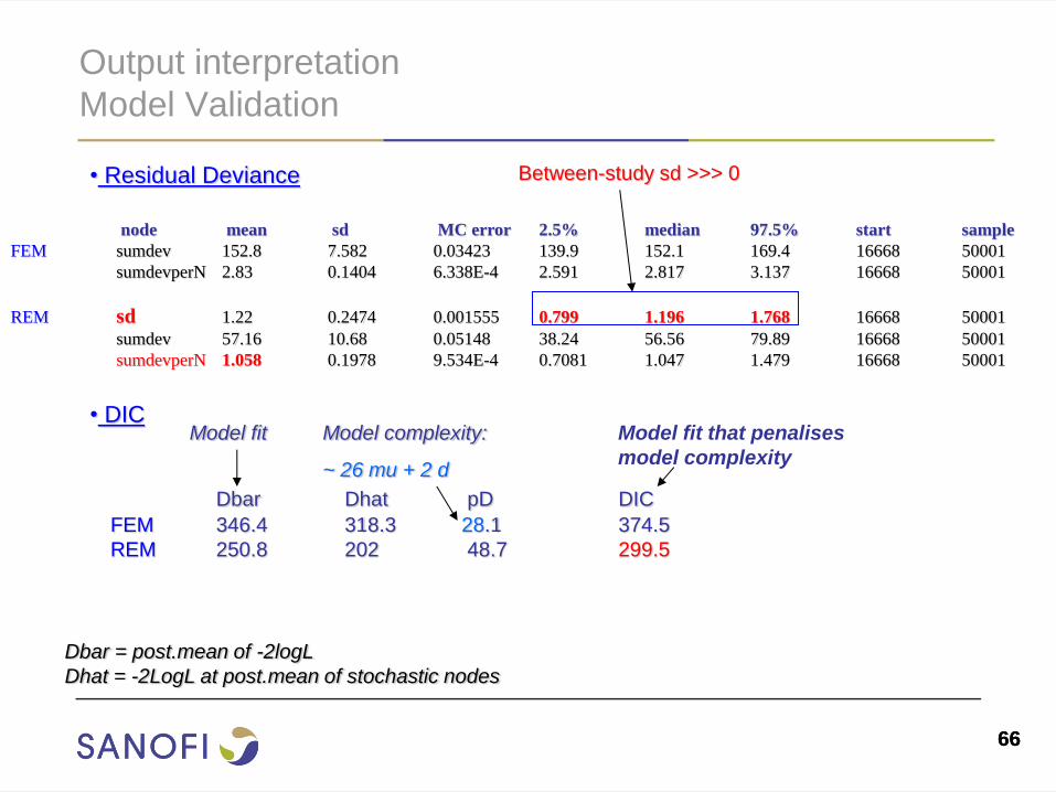
Output interpretation
Model Validation
• Residual Deviance
node mean sd MC error 2.5% median 97.5% start sample
FEM sumdev 152.8 7.582 0.03423 139.9 152.1 169.4 16668 50001
sumdevperN 2.83 0.1404 6.338E-4 2.591 2.817 3.137 16668 50001
REM sd 1.22 0.2474 0.001555 0.799 1.196 1.768 16668 50001
sumdev 57.16 10.68 0.05148 38.24 56.56 79.89 16668 50001
sumdevperN 1.058 0.1978 9.534E-4 0.7081 1.047 1.479 16668 50001
Between-study sd >>> 0
Dbar Dhat pD DIC
FEM 346.4 318.3 28.1 374.5
REM 250.8 202 48.7 299.5
• DIC
Dbar = post.mean of -2logL
Dhat = -2LogL at post.mean of stochastic nodes
Model complexity:
~ 26 mu + 2 d
Model fit Model fit that penalises
model complexity
67 67
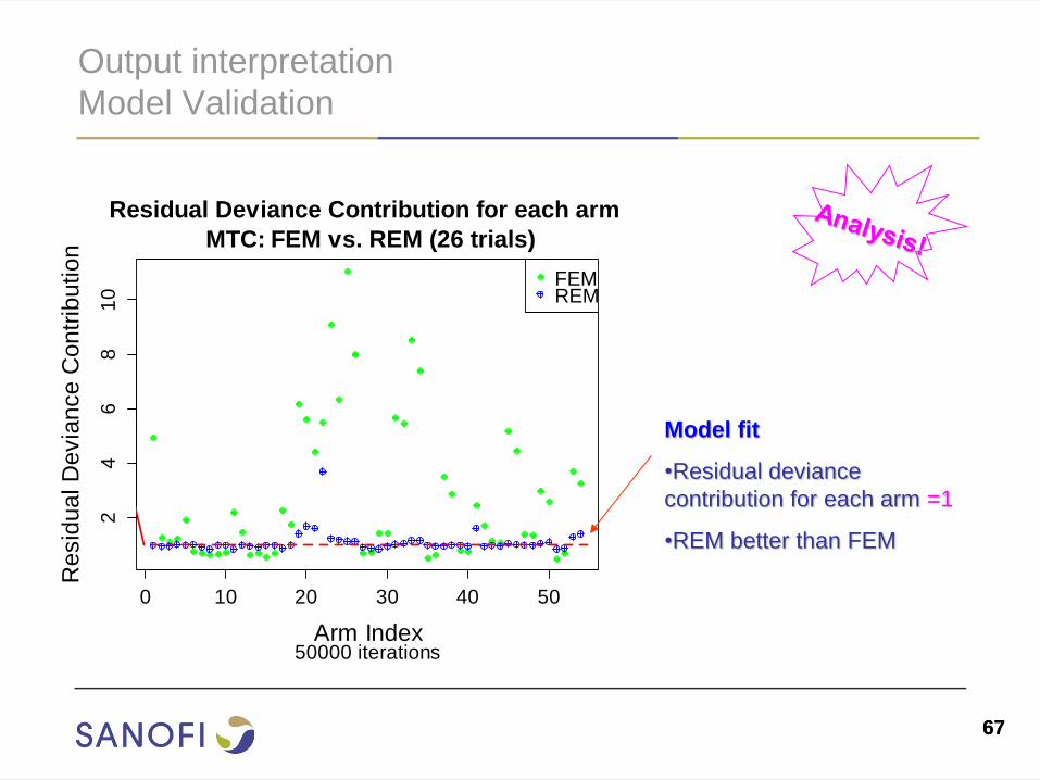
Output interpretation
Model Validation
0 10 20 30 40 50
24
68
10
Residual Deviance Contribution for each arm
MTC: FEM vs. REM (26 trials)
50000 iterationsArm Index
Resid
ua
l D
evia
nce
Con
trib
utio
n
FEMREM
Model fit
•Residual deviance
contribution for each arm =1
•REM better than FEM
68 68
Conclusion
● Modelling:
● Linear predictor model with additivity effects
● Making sure convergence before model fit assessment
● Between-trial heterogeneity (REM or meta regression) can only be well estimated with enough trials
● Guideline requires inconsistency with clear standards for identification of inconsistency but dealing with inconsistency are currently lacking
● Maintain the randomization within a study and integrate the difference / relative effect across different studies
● But cannot replace direct evidence
● Based on aggregate data: may not enough powerful to detect difference:
• NMA combing individual patient and aggregate data
●Not always respects all basic assumptions: similarity, homogeneity and consistence.
●Rather comprehensive sensitivity analyses supports the robustness of the findings
●Interpret results under such context
●High trend of HTA’s demand in case of direct evidence lack
69 69
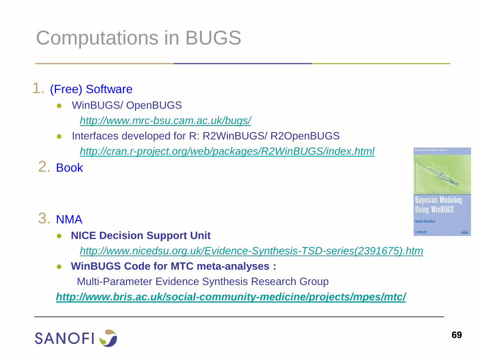
Computations in BUGS
1. (Free) Software
● WinBUGS/ OpenBUGS
http://www.mrc-bsu.cam.ac.uk/bugs/
● Interfaces developed for R: R2WinBUGS/ R2OpenBUGS
http://cran.r-project.org/web/packages/R2WinBUGS/index.html
2. Book
3. NMA
● NICE Decision Support Unit
http://www.nicedsu.org.uk/Evidence-Synthesis-TSD-series(2391675).htm
● WinBUGS Code for MTC meta-analyses :
Multi-Parameter Evidence Synthesis Research Group
http://www.bris.ac.uk/social-community-medicine/projects/mpes/mtc/

Computations in BUGS
70

71 71
Bibliography
● Lu G, Ades AE. Journal Of The American Statistical Association, 2006
● J. Spiegelhalter : Bayesian approches to random-effects meta-analysis : A comparative study. Statist.
Med. 1995 ; 14 : 2685-2699
● Dias S, Welton N, Sutton A, Ades AE. NICE DSU Technical Support Document 2: A Generalised
Linear Modelling Framework for Pairwise and Network Meta-Analysis of Randomised Controlled Trials.
2012
● CADTH. Indirect Evidence: Indirect Treatment Comparisons in Meta-Analysis. 2009
● Interpreting Indirect Treatment Comparisons and Network Meta-Analysis for Health-Care
● Decision Making: Report of the ISPOR Task Force on Indirect Treatment Comparisons. Good
Research Practices: Part 1
● Dias, S., N. J. Welton, A. J. Sutton, D. M. Caldwell, G. Lu and A. Ades (2011). "NICE DSU technical
support document 4: inconsistency in networks of evidence based on randomised controlled trials."
Decision Support Unit.

72 72
The end
Thank you for your attention
Q & A