Bayesian outlier detection in Geostatistical models · Bayesian outlier detection in Geostatistical models ... In the classical linear regression model, the residuals are usually

Bayesian outlier detection in Geostatistical models

Viviana G. R. Loboa and Thaıs C. O. Fonsecab

aFluminense Federal University, Rio de Janeiro, Brazil; bFederal University of Rio deJaneiro, Rio de Janeiro, Brazil

ARTICLE HISTORY

Compiled October 4, 2016

ABSTRACT

This work considers residual analysis and predictive techniques in the identifi-cation of individual and multiple outliers in geostatistical data. The standardizedBayesian spatial residual is proposed and computed for three competing models:the Gaussian, Student-t and Gaussian-log-Gaussian spatial processes. In this con-text, the spatial models are investigated regarding their plausibility for datasetscontaminated with outliers. The posterior probability of an outlying observation iscomputed based on the standardized residuals and different thresholds for outlierdiscrimination are tested. From a predictive point of view, methods such as theconditional predictive ordinate, the predictive concordance and the Savage-Dickeydensity ratio for hypothesis testing are investigated in the identification of outliers inthe spatial setting. For illustration, contaminated datasets are considered to accessthe performance of the three spatial models in the identification of outliers in spatialdata.

KEYWORDSResidual analysis; Spatial statistics; Outlier detection; Predictive performance;Contaminated datasets.

1. Introduction

From a theoretical point of view, statistical inference goes beyond parameter estima-tion and prediction [see 20, page 343]. Often, tests are performed regarding modelparameters which are based on models that are not adequate to the data under study.That is, model adequacy checking should not be based on model parameter testing.Some verification of model goodness of fit is then called for. From a Bayesian perspec-tive, the issue is the same, statements are done regarding the posterior distributionwhich is also based on the chosen sampling distribution for the data. The usual modelcriticism is done throught model comparison and prediction for few out of sample ob-servations. Often, these model checkings are not able to access whether the assumedmodel is plausible for the data. This work is motivated by the idea that model de-termination or checking should be based on residual analysis, predictive performanceand outlier detection. [14] suggest a general framework based on goodness of fittingchecking from a Bayesian point of view. This is the kind of approach this paper aims

CONTACT Thais C. O. Fonseca, Av. Athos da Silveira Ramos, Centro de Tecnologia, Bloco C Sala C114

D, IM-UFRJ, CEP 21941-909, Rio de Janeiro, Brazil, Email: [email protected]

to pursue for spatially correlated data modelling.An stylized fact of statistical applications in general is that if the data contain

aberrant observations, the estimated model might not be a good representation of thephenomenon under study, leading to poor predictions for out of sample observations.An important tool in the identification of atypical observations is the residual analysis.In the classical linear regression model, the residuals are usually defined as the differ-ence between observed and fitted values. In the Bayesian context, [4] defines an outlieras an observation with large random error generated by the sampling distribution ofthe data. In this case, the discrepant observation might be detected through the pos-terior distribution of these random errors. On the other hand, [11] considers an outlierany observation which was not generated by the mechanism generating the majorityof the data. In the independent data setting several papers discussed the detectionof outliers such as [23] which considers heavy tailed distributions defined throught aGaussian mixture model to accommodate and detect outliers in a regression setup.

The focus of this work is the analysis and detection of regional outliers which mightbe neightboors in space. Indeed, in the spatial statistics context the issue of outlierdetection or modeling is even more important than in the independent case. Predic-tion at new locations is usually based on krigging ideas and krigging predictors arewell known to be affected by outliers as they are obtained as linear combination ofobservations. In geostatistics, an outlier may have a strong effect in the prediction ofits neighboors when the observed value for the process at this location is much higheror lower than expected for that region in space. [5] comment that, in applied settings,even small changes in some regions in space might cause large differences between thepredicted and observed process. Observations in these regions should not be discartedas this might cause bias in the estimation of parameters and predictions [5, page 221].

Several papers have proposed robust alternatives or modifications of usual krigingpredictor. [9] proposed a model to robustify the kriging predictor by defining themodel for geostatistical data as a mixture of a spatial process and a contaminationprocess. In this proposal each site has a corresponding contamination variable whichindicates whether the site is contaminated or not. The optimal predictor in this casedepends on weights which will be affected by the contamination variables. However, thepredictor is unfiasible in practice and an approximation is considered. [18] proposed theGaussian-Log-Gaussian process which is able to capture heterogeneity in space througha mixing process used to increase the Gaussian process variability. This proposal isan alternative to the usual Gaussian process which is very sensitive to outliers. Themixture approach is able to both accommodate and detect outliers. The detectionstep is done throught hypothesis testing. In particular, [18] considered Bayes factorsfor that purpose. Notice however that hypothesis testing based on Bayes Factors willdepend on the loss function considered to reach a conclusion regarding the outlyingobservation. Thus, it might be useful to consider other identification techniques jointlywith the hypothesis testing.

A potentially robust alternative model for spatial processes is the Student-t processdiscussed in [21]. However, the Student-t process inflates the variance of the wholeprocess in the presence of outliers in the data and does not allow for individual orregional outlier detection as it does not allow for different kurtosis behaviours acrossspace.

In the literature few proposals deal with model checking or validation for correlateddata. In particular, few papers discuss model checking for random functions. [15] de-scribes a deletion scheme for models based on correlated observations. [10] and [16]proposed graphical diagnostics for time series models. [16] propose a rotated residual

2

for independent and time series data which has good asymptotic properties. And [2]propose Bayesian diagnostics for computer models through Cholesky decompositionsof the covariance matrix. The proposal results in numerical and graphical tools formodel checking in the context of Gaussian processes.

This work proposes to extend the Bayesian residual approach of [4] to accomodatespatially correlated observations. In particular, the data is assumed to vary continu-ously in a spatial domain of interest D and residual analysis and predictive tecniquesare investigated aiming to identify potential outliers or regions of larger variability inthe data. The chosen model is crucial in the definition of residuals, thus this paperconsiders a flexible mixture model for geostatistical data.

The paper is organized as follows. Section 2 describes three competing modelsfor geostatistical data analysis: the Gaussian process, the Student-t process and theGaussian-Log-Gaussian process. Section 3 presents the proposed spatial residual foroutlier identification, discusses the predictive approach and defines a new measure foroutlier detection which is based on cross-validation ideas. In addition, the hypothesistest for outlying observations in the context of Gaussian-Log-Gaussian processes ispresented for comparison with the other proposed techniques. Section 4 illustrates themethods for outlier detection with contaminated datasets and section 5 concludes.

2. Mixture modelling for outlier detection

As follows we consider a mixture model which mimics a mechanism for outlier gener-ation in a geostatistical context. Consider the spatial process defined in s ∈ D suchthat

Z(s) = xT (s)β + σZ(s)

λ(s)1/2+ ε(s), (1)

where Z(s) is a Gaussian process defined in s ∈ D with zero mean and correlationfunction ρ(s, s′), s, s′ ∈ D. The process Z(s) is independent of ε(s) ∼ N(0, τ2) whichmodels the measurement error parametrized by τ2, the nugget effect. The mean func-tion depend on covariates xT (s) = (x1(s), . . . , xk(s)) and β, a vector of regressioncoefficcients. The process λ(s) is the mixing process allowing for spatial heterogeneity.If λ(s) 6= 1 the process Z(s) is non-Gaussian. In the absence of nugget effect, theprocess λ(s) must be correlated to induce mean squared continuity of Z(s) [see 18,for details]. Consider s1, . . . , sn spatial locations in D and Z = (Z(s1), . . . , Z(sn)) theobserved data at these locations. The models investigated in this work are detailed asfollows.

(A) Gaussian model: we set λ(s) = 1, ∀s ∈ D as a benchmark. The distributionof Z is

Z | β, σ2, τ2, θ ∼ Nn(Xβ, σ2Σθ + τ2In), (2)

Σθ(i,j) = ρ(si, sj) = ρ(si, sj ; θ), i,j=1,. . . ,n.

(B) Student-t model: define λ(s) = λ, ∀s ∈ D such that λ | ν ∼ Ga(ν/2, ν/2).

3

Then, by marginalization, the distribution of Z is

Z | β, ν, σ2, τ2, θ ∼ Student-t(ν,Xβ, σ2Σθ + τ2In). (3)

Similar to the Gaussian process, the Student-t process has the advantageof depending on the mean and covariance functions only for its definition.Details about the Student-t process in a non-Bayesian context may be seen in[21]. Appendix A presents the likelihood function resulting from this model.Appendix B.1 presents the posterior inference considered which is based onJeffreys independent prior distribution for the unknown degree of freedomparameter as proposed by [7].

(C) Gaussian-Log-Gaussian model: consider ln(λ) | ν, θ ∼ Nn

(−ν

2 1n, νΣθ

)with

λ = (λ(s1), . . . , λ(sn)). Then, the distribution of Z is

Z | β, σ2, τ2,Λ, θ ∼ Nn(Xβ, σ2(Λ−1/2ΣθΛ−1/2) + τ2In), (4)

with Λ = diag(λ). Properties, estimation and predition for the GLG model areintroduced in [18] and extendend to the space-time case in [8]. Appendix B.2presents the posterior inference for the model parameters.

Although the Student-t model allows for variance inflation, it increases the kurtosis forthe process in every location and does not allow for individual changes in variability.For the GLG model, if λ(sk) is close to one then the observation is not consideredan outlier. However values of λ(sk) close to zero indicate outlying observation. Themarginal kurtosis for the process Z(s) is given by κ = 3 exp{ν} implying that ν → 0results in the Gaussian case with kurtosis 3 and large values of ν indicate fatter tailsthan the Gaussian model.

In this paper, we investigate the three models in the detection of outliers in spatialdata. For that purpose, we compare the performance of methods for outlier detectionin the context of correlated data. Furthermore, we propose a new measure based oncross validation ideas and extend the Bayesian residual proposed by [4] to the spatialcontext.

3. Outlier detection in spatial modelling

In this section we describe three approaches to outlier detection in spatial modelling:the posterior probability computation of a large residual, predictive techniques such asthe predictive concordance and the hypothesis testing for the latent mixing variables.

3.1. Bayesian residual analysis

Definition 3.1. Consider Z = (Z(s1), . . . , Z(sn)) observations at n spatial locationsof the the spatial process {Z(s), s ∈ D} as defined in (1) such that Z | β, σ2,Λ ∼Nn(Xβ, σ2(Λ−1/2ΣθΛ

−1/2)), with Λ = diag(λ). Then the standardized Bayesian spa-tial residual for the mixture model without nugget effect is

r = σ−1Λ1/2Σ−1/2θ (Z −Xβ) (5)

4

If the errors are Gaussian distributed then approximately 95% of the individualresiduals are expected to be in the interval [−2, 2]. If an observation is out of thisinterval there is some evidence that this observation could be an outlier. In order todetect outlying observations, [4] define the posterior probability that an observationis an outlier as pi = P (|ri| > t | z). According to [4] the value of t can be chosen sothat the prior probability of no outliers is large, say 0.95. The constant t is chosento be Φ−1(0.5 + 0.5(0.951/n)). Any observation with posterior probability of being anoutlier larger than the prior probability 2Φ(−t) would be suspect. In a context ofbinary regression [1] and [22] consider t = 0.75.

In the geostatistical setting, we will set the value of t to different constants andverify by simulation for several scenarios how the mixture process is sensitive to thischoice. It is expected that not all values used for regression model will have goodperformance in the correlated data context.

Furthermore, we investigate the joint posterior probability of two observations beingoutliers. This is a phenomena which is expected in spatial applications. In particular,due to spatial correlation of observations and smoothness of the spatial process, twoobservations which are close together are expected to have large errors if there is amechanism causing outliers in the spatial region where these two observations arelocated. Thus, the joint posterior probability that the pair (ri, rj) is a regional ormultiple outlier is

pij = P (|ri| > t, |rj | > t | z). (6)

In particular, the variance process 1/λ(s) in the GLG model is considered to becorrelated with ln(λ) | ν ∼ Nn

(−ν

2 1n, νΣθ

). Thus, if an individual outlier is detected

then this indicates that observations in the close neighborhood are potential outliers.This could be verified computing pij . [8] extends this proposal by allowing for in-dependent outlying observations through individual nugget effects for each location.This approach is not discussed in this work as replicates in time would be required forparameter estimation.

3.2. Predictive approach

An alternative definition of an outlier was given by [13]. An observation is said aberrantor discrepant if it is in the tails of the predictive posterior distribution. The authordefine the Predictive Concordance for observed value zi as

pci = P (zrep > zi) =

∫ ∞zi

p(zrep)dzrep, (7)

with zrep an imaginary observation and p(zrep) the predictive distribution of zrep. Thismeasure is similar to the Bayesian p-value. [13] says that any observation which is inthe 2.5% tail of p(zrep) should be considered an outlier. The percentage of outliers inthe data should be smaller than (100−C)% where C% is the Predictive Concordance.[13] suggests the achievement of 95% predictive concordance for model adequacy.

Notice that the pci is computed based on the full predictive distribution, however, tocheck whether zi is an outlier it actually uses zi to obatin the predictive distribution.Thus, the model might predict this observation better than it should if zi was notin the data. The leave-one-out predictive distribution obtained by removing zi fromthe data might give better information about model performance to predict zi. [13]

5

proposed the Conditional Predictive Ordinate or CPO

CPOi = p(zi|z(i)) =

∫p(zi|θ)p(θ|z(i))dθ (8)

where zi represents a observed value from z and z(i) represents the vector z withoutzi. Notice that p(zrep|z(i)) represents the predictive density of a new observation giventhe dataset which does not include zi. Values of CPOi close to zero suggest thatobservation i is a potential outlier. [19] comments that althought the CPOi could beused as a surprise index it might return similar values for all observations failling inidentifying outlying observations. In these situations [19] suggest a new measure calledRatio ordinate measure (ROM) which is the CPO standardized by max{p(zrep|z(i))}.This measure aims at given more realistic indications of outliers in a dataset.

Following the ideas based on predictive distributions and Predictive Concordancethis work proposes a measure for spatial data which is based on cross-validation ideas.

Definition 3.2. The p-value from CPO is defined as

CPOpi = P (zrep > zi | z(i)) (9)

The proposed measure is similar to the predictive concordance however it leaves ziout of the dataset used for parameter estimation. This proposal checks if the observedvalue zi is in accordance with the predictive distribution which was obtained excludingzi from the dataset. [12] argues that zi should not be used to determine the predictivedistribution for model checking. For this measure, values of zi in either tails of thepredictive distribution will indicate that zi is an outlier.

3.3. Savage-Dickey ratio test

A different approach to outlier detection considers inference directly in the mixingprocess λ(s), s ∈ D. Thus, λ(sk) close to one indicates that observation at locationsk is not an outlier. Thus, the model that considers λ(sk) = 1 could be compared tothe model which considers free λ(sk). This model comparison could be done throughBayes Factors after fitting both models to the data. An alternative to fitting bothmodels and then computing the Bayes Factor [17] is to consider only the model withfree λ(sk) and the Savage-Dickey density ratio to approximate the Bayes Factor forthe hypothesis that λ(sk) = 1 versus λ(sk) 6= 1. The Savage-Dickey density ratio wasproposed by [6] and can be used when the restriction in the parameter being tested inthe null hypothesis is not in the boundary of the parameter domain.

According to [18] the hypothesis testing is useful to indicate outliers in the data orregions with larger variability in space.

The resulting approximation for the Bayes Factor for each location sk is given by

Rk =p(λ(sk) | z)

p(λ(sk)) |λ(sk)=1

(10)

with the ratio Rk being favorable to the model with λ(sk) = 1 and all the other λfree against the model with free λ(sk). Thus, small values of Rk (much smaller than1) will indicate outliers. [17] give some guidelines for interpretation of Bayes Factors.According to the authors, values of Rk smaller than 0.10 give strong evidence that

6

λ(sk) 6= 1. Values between 0.1 and 0.3 give substancial evidence that λ(sk) 6= 1, whilevalues between 0.3 and 1 give some evidence but are not very conclusive.

4. Application

4.1. Simulated dataset

In this subsection the three models presented in section 2, Gaussian model (GM),Student-t model (STM) and Gaussian log Gaussian model (GLGM) are consideredin the identification of outliers in contaminated datasets. In the context of dynamicalmodels [23] comments that contaminated datasets, simulated originally from Gaus-sian distribution and then contaminated to characterize aberrant observations, area useful tool to evaluate the performance of robust models. In this simulated studywe consider the ideia of Gaussian data contamination in the context of spatial data.Three scenarios of contamination are presented: no contamination, weak contamina-tion and moderate contamination as presented in table 1. Observations in the weakscenario were contaminated summing a random increment uσ such that σ is the obser-vational standard deviation and u ∼ Uniform(1, 3.5) for observations 1 and 20 andu ∼ Uniform(1, 2.5) for observation 6. While in the moderate scenario the randomincrement was generated from u ∼ Uniform(1, 3.5) for observations 1, 13, 15, 16, 20,30, from u ∼ Uniform(1, 2.5) for observations 6 and from u ∼ Uniform(1, 6.5) forobservations 29. The locations considered for data simulation and contamination arepresented in figure 1. Notice that some of the contaminated locations are neighboorsin space.

Assume that Z(s) is a spatial process in D. Consider data observed in n = 30spatial locations z = (z(s1), . . . , z(sn))′. Then, z is simulated from fn(µ, σ2Σθ), suchthat µi = µ(si) = β0 + β1lati + β2longi and covariance matrix Σθ with componentsΣθ(ij) = exp{−||si−sj ||/φ}, with lati and longi the latitude and longitude for locationi, respectively. The parameter values considered for simulation were β0 = 6, 716, β1 =2, 7, β2 = −1, 808 for the mean vector, and σ = 1, φ = 0, 61 for the covariance matrixparameters.

Samples from the posterior distribution for the parameters of interest are obtainedby Markov Chain Monte Carlo simulation. Some details about posterior simulationare presented in the Appendix B. For more details of sampling from parameters fromthese models see [18].

In this simulated example, it is expected that contaminated observations have largeposterior residual probabilities while non-contaminated observations should have smallresidual probabilities. For the limiar t three choices were considered: t1 = 0.75, t2 =2, t3 = 3.1 with t1 from [1] and [22], t2 an arbitrary intermediate constant and t3based on [4]. Figure 2 presents the posterior distribution for the residuals for eachmodel and scenario of contamination. Note that in scenario 1 (first row), which hasno contamination, the three models have a desirable behavior and do not indicateoutlying observations in the data. In scenario 2, only the GLG model identifies theobservation 6 as an outlier and the three models identify observations 1 and 20. Inthe scenario 3, with moderate outliers the GLG model is the only model which hasrealistic posterior probabilities of large residuals for all the contaminated observationswhile the Gaussian and Student-t models fails to identify most of these observations.

For the actual identification of outlying observations the limiar t1, t2 and t3 areconsidered. Table 2 presents the posterior probabilities of atypical observations for

7

t3, pi(|ri| > t3 | z). In the scenario 1 (no contamination) it is expected that theprobabilities of outliers are small. However, if limiars t1 and t2 are considered theseprobabilities are unexpectedly high. Thus, this suggests that only limiar t3 should beconsidered for outlier identification in the spatial data scenario simulated in this work.

Contaminated observations in scenarios 2 and 3 are presented in tables 3 and 4. TheGLG model give large probabilities of outliers for the contaminated observations whilegives small probabilities for observations which were not contaminated. The Gaussianand Student-t models fail to identify the contaminated observation 6 as an outlier. Inscenario 2 with weak contamination, the GLG model gave a probability of 0.228 forobservation 6 being an outlier while the Gaussian and Student-t models had 0.000 and0.001, respectively. For instance, in scenario 3, the models gave probabilities for thecontaminated observation 30 of being an outlier 0.000 (GM),0.042 (STM) and 0.795(GLGM). Thus, the GLG was the only model to correctly identify all the outlyingobservations in the data. Notice that in this simulated example no observation wasclassified as an outlier when it was not contaminated.

In addition, scenarios 2 and 3 are investigated for multiple outliers. In the context ofgeostatistical data, it is expected that outliers are not observed isolated but in a regionin space. In this direction, the joint probability of multiple outliers was computed pijas in equation (6). Table 5 presents the probabilities for a set of pairs in the sampledlocations and the corresponding posterior correlation.

Once again the GLG model is the only model which correctly give reasonably largeposterior probabilities for all pairs of outliers in scenario 2. The Gaussian and Student-t models give reasonably large probabilities for the pair (1, 20) however give close tozero posterior probability for the pair (1, 6) and (6, 20). This is explained by the factthat the Gaussian and Student-t model do not model heterogeneity in space.

Table 6 presents the results for scenario 3. Only the pair (1, 15) have reasonablylarge posterior probabilities of being multiple outliers in the Gaussian and Student-tmodels althought all the other pairs in the table have very large spatial correlation.The GLG model correctly indicates all the contaminated pairs as multiple outliers.

As follows, the predictive measures were computed for the contaminated scenarios.In particular, tables 7 to 9 present the pci as presented in (7) for the scenarios: nooutliers, weak outliers and moderate outliers, respectively. If the observation is notin the 5% tail it is not classified as outlier. Observation in the tail are indicated aspotential outliers.

The CPO is misleading in scenario 1, resulting in cpoi of 0.006 (GM), 0.000 (STM)and 0.137 (GLG) for observation 27 which would indicate an outlier, however, noobservation was contaminated in this scenario. The predictive concordance pci and theproposed p-value based on CPO behave as expect and do not indicate any observationas an outlier in this scenario. For scenario 3, the advantages of the proposed p-value iseven more evident. In scenario 2, observation 27 was not contaminated however, cpoiwas 0.039 (GM), 0.000 (STM) and 0.000 (GLGM) indicating an outlier. While theproposed CPOp were 0.769 (GM), 0.898 (STM) and 0.385 (GLGM) which correctlydo not indicate outlying observation. The predictive concordance also give reasonableresults for observation 27: 0.742 (GM), 0.651 (STM) and 0.486 (GLGM). In scenario 3,while the cpoi is smaller than 10−4 for observation 27 (non-contaminated) indicatingan outlier, the CPOp is 0.281 and the pci is 0.402. An analogous behaviour is obtainedfor observation 3 which was not contaminated.

Table 10 indicate strong evidence that λi 6= 1 for all contaminated observations inthe hypothesis testing for scenario 2. For instance, for observation 1, the Bayes Factorin favour of free λi is 0.011 giving strong evidence of free λ(s) in this location. The

8

results for scenario 3 with moderate contamination are presented in table 11. The ratioRi correctly indicates all contaminated observation as outliers such as observation 6which has Ri = 0.05 indicating strong evidence of an outlying observation.

Table 1. Contamination scenarios.

Scenario 1 no outliers in the dataScenario 2 weak outliers: 3 points were contaminatedScenario 3 moderate outliers: 8 points were contaminated

Table 2. Standardized residuals and posterior probabilities of outliers, pi(|ri| > t|z) for scenario 1 (no outlier).

Scenario 1 (no outlier)Gaussian Student-t GLG

i ri p(t1)i p(t2)i p(t3)i ri p(t1)i p(t2)i p(t3)i ri p(t1)i p(t2)i p(t3)i1 0.730 0.489 0.033 0.738 0.530 0.044 1.170 0.742 0.298 0.0623 -0.575 0.403 0.020 -0.547 0.420 0.021 -0.467 0.519 0.084 0.0116 -0.100 0.296 0.002 -0.033 0.269 0.006 -0.181 0.474 0.073 0.00815 0.759 0.536 0.039 0.794 0.551 0.058 0.003 1.372 0.772 0.301 0.07220 0.495 0.391 0.020 0.495 0.392 0.024 0.928 0.663 0.193 0.03027 -0.724 0.517 0.082 0.003 -0.580 0.480 0.058 0.002 -0.691 0.645 0.208 0.03830 0.074 0.309 0.007 0.143 0.317 0.007 0.443 0.519 0.111 0.009

aPosterior probabilities smaller than 10−3 are omitted from the table.

Table 3. Standardized residuals and posterior probabilities of outliers, pi(|ri| > t|z) for scenario 2 (weak outliers).

bold-faced observations represent contaminated observations.

Scenario 2 (weak outlier)Gaussian Student-t GLG

i ri p(t1)i p(t2)i p(t3)i ri p(t1)i p(t2)i p(t3)i ri p(t1)i p(t2)i p(t3)i1 3.711 1.000 0.998 0.797 3.731 1.000 0.995 0.839 5.426 1.000 1.000 0.9973 -0.796 0.524 0.007 -0.639 0.455 0.016 0.222 0.432 0.053 0.0056 0.920 0.618 0.010 1.050 0.698 0.092 0.001 2.364 0.965 0.664 0.22815 0.680 0.473 0.004 0.756 0.522 0.044 1.883 0.877 0.436 0.11220 2.622 0.999 0.848 0.114 2.668 0.999 0.863 0.299 4.300 0.999 0.995 0.90427 -0.871 0.548 0.060 -0.592 0.505 0.053 0.001 0.137 0.578 0.143 0.03330 -0.056 0.152 0.102 0.273 0.005 1.058 0.667 0.209 0.045


9

Table 4. Standardized residuals and posterior probabilities of outliers, pi(|ri| > t|z) for scenario 3 (moderate

outliers). Bold-faced observations represent contaminated observations.

Scenario 3 (moderate outlier)Gaussian Student-t GLG

i ri p(t1)i p(t2)i p(t3)i ri p(t1)i p(t2)i p(t3)i ri p(t1)i p(t2)i p(t3)i1 3.71 1.000 0.979 0.344 3.080 0.999 0.925 0.456 5.338 1.000 1.000 0.9863 -0.796 0.756 0.008 -0.958 0.630 0.044 0.001 0.507 0.478 0.072 0.0076 0.920 0.114 0.472 0.345 0.017 2.628 0.969 0.733 0.31015 0.680 1.000 0.993 0.723 3.817 1.000 0.994 0.805 5.734 1.000 1.000 0.99620 2.622 0.997 0.563 0.002 2.135 0.971 0.574 0.066 4.273 1.000 0.989 0.89627 -0.871 0.959 0.335 0.023 -1.459 0.808 0.254 0.017 0.702 0.624 0.244 0.06730 -0.056 0.965 0.192 1.937 0.957 0.443 0.042 3.988 1.000 0.975 0.795


Table 5. Posterior probabilities of multiple outliers pij =

p(|ri| > t3, |rj | > t3|z) and posterior correlation ρij for ri andrj , for each model in scenario 2.

i,j Gaussian Student-t GLG Correlation ρij1,6 0.001 0.228 0.8691,20 0.114 0.299 0.904 0.9506,20 0.001 0.227 0.854

aPosterior probabilities smaller than 10−3 are omitted from thetable.

Table 6. Posterior probabilities of multiple outliers pij = p(|ri| >t3, |rj | > t3|z) and posterior correlation ρij for ri and rj , for eachmodel in scenario 3.

i,j Gaussian Student-t GLG Correlation ρij1,15 0.307 0.433 0.982 0.8341,20 0.002 0.066 0.896 0.9581,29 0.006 0.603 0.8501,30 0.042 0.794 0.8476,20 0.307 0.87515,20 0.002 0.066 0.893 0.933

aPosterior probabilities smaller than 10−3 are omitted from thetable.

Table 7. pci,cpoi, CPOpi for some observations in the sample. Bold-faced observationsrepresent the contaminated observations.

Scenario 1Gaussian Student-T GLG

Obs. pci cpoi CPOpi pci cpoi CPOpi pci cpoi CPOpi1 0.271 0.145 0.257 0.297 0.039 0.201 0.252 0.001 0.2613 0.685 0.200 0.712 0.680 0.016 0.769 0.611 0.259 0.26115 0.278 0.112 0.262 0.267 0.011 0.197 0.226 0.101 0.23520 0.337 0.227 0.341 0.361 0.017 0.286 0.307 0.174 0.29127 0.678 0.006 0.700 0.647 0.000 0.873 0.643 0.137 0.627

aValues smaller than 10−4 are omitted from the table.

Table 8. pci,cpoi, CPOpi for some observations in the sample. Bold-faced observations repre-

sent the contaminated observations.


Obs. pci cpoi CPOpi pci cpoi CPOpi pci cpoi CPOpi1 0.001 0.001 0.013 0.0193 0.767 0.2395 0.780 0.700 0.0577 0.886 0.457 0.239 0.50715 0.264 0.281 0.243 0.269 0.173 0.199 0.177 0.232 0.27720 0.009 0.003 0.001 0.016 0.031 0.004 0.11027 0.742 0.039 0.769 0.651 0.898 0.486 0.385


10

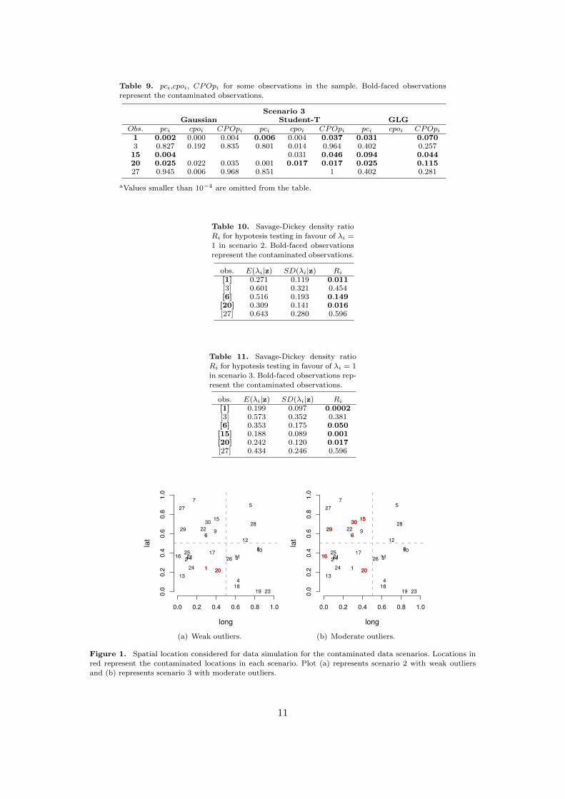
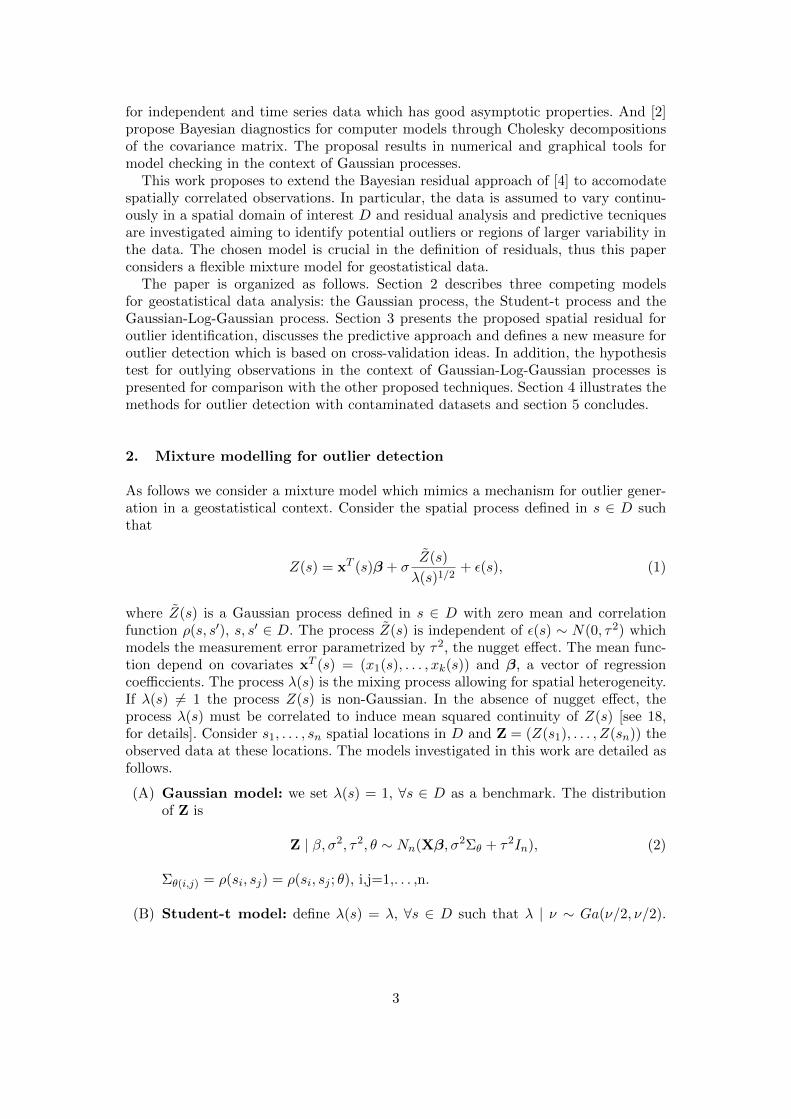
Table 9. pci,cpoi, CPOpi for some observations in the sample. Bold-faced observations

represent the contaminated observations.


Obs. pci cpoi CPOpi pci cpoi CPOpi pci cpoi CPOpi1 0.002 0.000 0.004 0.006 0.004 0.037 0.031 0.0703 0.827 0.192 0.835 0.801 0.014 0.964 0.402 0.25715 0.004 0.031 0.046 0.094 0.04420 0.025 0.022 0.035 0.001 0.017 0.017 0.025 0.11527 0.945 0.006 0.968 0.851 1 0.402 0.281


Table 10. Savage-Dickey density ratio

Ri for hypotesis testing in favour of λi =1 in scenario 2. Bold-faced observations

represent the contaminated observations.

obs. E(λi|z) SD(λi|z) Ri

[1] 0.271 0.119 0.011[3] 0.601 0.321 0.454[6] 0.516 0.193 0.149[20] 0.309 0.141 0.016[27] 0.643 0.280 0.596

Table 11. Savage-Dickey density ratio

Ri for hypotesis testing in favour of λi = 1

in scenario 3. Bold-faced observations rep-resent the contaminated observations.

obs. E(λi|z) SD(λi|z) Ri

[1] 0.199 0.097 0.0002[3] 0.573 0.352 0.381[6] 0.353 0.175 0.050[15] 0.188 0.089 0.001[20] 0.242 0.120 0.017[27] 0.434 0.246 0.596

long

lat

0.0 0.2 0.4 0.6 0.8 1.0

0.0

0.2

0.4

0.6

0.8

1.0

1

2 3

4

5

6

7

8

9

10

11

12

13

14

15

1617

1819

20

21

22

23

24

25

26

27

2829

30

1 20

6

(a) Weak outliers.

long

lat

0.0 0.2 0.4 0.6 0.8 1.0

0.0

0.2

0.4

0.6

0.8

1.0

1

2 3

4

5

6

7

8

9

10

11

12

13

14

15

1617

1819

20

21

22

23

24

25

26

27

2829

30

1 20

6

15

29

30

16

(b) Moderate outliers.

Figure 1. Spatial location considered for data simulation for the contaminated data scenarios. Locations inred represent the contaminated locations in each scenario. Plot (a) represents scenario 2 with weak outliers

and (b) represents scenario 3 with moderate outliers.

11

(a) GM. (b) STM. (c) GLGM.

(d) GM. (e) STM. (f) GLGM.

(g) GM. (h) STM. (i) GLGM.

Figure 2. Posterior distribution for the residuals in each scenario: no contamination (first row), weak con-tamination (second row) and moderate contamination (tird row).

12

5. Conclusions

The idea that the Student-t process would result in robustness to outliers is misleadingas the degree of freedom is the same in all spatial locations leading to inflation in theglobal variance. However, the model does not allow for actual detection of regions withaberrant observation in spatial data. These ideas were discussed in [3] and [18]. Thiswork adds in this direction by presenting simulation for spatial contaminated datasetsand obtaining no outlier detection for most of outliers in the data using the Student-tmodel. The Student-t process for spatial data is not able to detect outliers either bymarginal probabilities or multiple detection procedures. The GLG mixture process, onthe other hand, indicates the outliers in all simulated scenarios for all detection toolspresented in this work. The residual analyses presented here is purely spatial in thesense that the mixture process is considered in space only. [8] considered a mixturemodel in space-time which is not exploit in this work.

The spatial Bayesian residuals, the proposed cross-validation p-value and theSavage-Dickey density indicate correctly the outliers and multiple outliers under theGLG model assumption. The CPO fail in identifying outliers for all models, givingmisleading indications for the contaminated scenarios. As an alternative, this workproposed the p-value based on the CPO, which is able to correctly detect aberrantobservations in the spatial data.

Acknowledgements

This work was part of the Master’s dissertation of Viviana G. R. Lobo under thesupervision of T. C. O. Fonseca. Lobo benefited from a scholarship from Conselho deAperfeicoamento de Pessoal de Nıvel Superior (CAPES), Brazil. T. C. O. Fonseca waspartially supported by Conselho Nacional de Desenvolvimento Cientıfico e Tecnologico(CNPq).

References

[1] Albert, J. and Chib, S. Bayesian residual analysis for binary response regression models.Biometrika, 82 (1995), pp. 747-759.

[2] Bastos, L. S. and OHagan, A. Diagnostics for Gaussian process emulators. Technometrics,51 (2008), pp. 425-438.

[3] Breusch, T. S., Robertson, J. C., and Welsh, A. H. The emperors new clothes: a critiqueof the multivariate t regression model. Statistica Neerlandica, 1997.

[4] Chaloner, K. and Brant, R. A Bayesian approach to outlier detection and residual analysis.Biometrika, 75, 4 (1988), pp. 651-659.

[5] Chiles, J.-P. and Delfiner, P. Modeling Spatial Uncertainty. New York: Wiley, 1999.[6] Dickey, J. The Weighted Likelihood Ratio, Linear Hypotheses on Normal Location Param-

eters. The Annals of Statistics, 42, 1 (1971), pp. 204-223.[7] Fonseca, T. C. O. and Ferreira, M. A. R. and Migon, H. S. Objective Bayesian analysis

for the Student-t regression model Biometrika, 95, 2 (2008), pp. 325–333.[8] Fonseca, T. C. O. and Steel, M. F. J. Non- Gaussian Spatiotemporal Modelling through

Scale Mixing. Biometrika, 98, 4 (2011), pp. 761-774.[9] Fournier, B. and Furrer, R. Automatic mapping in the presence of substutive errors: a

robust kriging approach. Applied GIS, 1 (2005), pp. 121-1216.[10] Fraccaro, R., Hyndman, R. J., and Veevers, A. Residual Diagnostic Plots for Checking

13

for Model Misspecification in Time Series Regression. Australian & New Zealand Journalof Statistics, 42, 4 (2000), pp. 463-477.

[11] Freeman, P. R. On the number of outliers in data from a linear model, 349365. Valencia:University Press, 1980.

[12] Gelfand, A. Model determination using predictive distributions with implementation viasampling-based methods. Technical report, Department of Statistics, Stanford University1992.

[13] Gelfand, A. Model Determination Using Samplings Based Methods. Chapman & Hall,Boca Raton, FL, 1996.

[14] Gelman, A., Meng, X.-L., and Stern, H. Posterior predictive assessment of model fitnessvia realized discrepancies. Statistica Sinica, 6 (1996), pp. 733-807.

[15] Hasllet, J. A Simple Derivation of Deletion Diagnostic Results for the General LinearModel with Correlated Errors. Journal of the Royal Statistical Society: Series B (StatisticalMethodology), 61, 3 (1999), pp. 603-609.

[16] Houseman, E. A., Ryan, L., and Coull, B. Cholesky Residuals for Assessing Normal Er-rors in a Linear Model with Correlated Outcomes. Journal of the American StatisticalAssociation, 99 (2004), pp. 383-394.

[17] Kass, R. E. and Raftery, A. E. Bayes Factors. Journal of the American Statistical Asso-ciation, 90, 430 (1995), pp. 773-795.

[18] Palacios, M. B. and Steel, M. F. J. Non-Gaussian Bayesian Geostatistical Modeling. Jour-nal of the American Statistical Association, 101, 474 (2006), pp. 604-618.

[19] Petit, L. The conditional predictive ordinate for the normal distribution. Journal of theRoyal Statistical Society: Series B (Statistical Methodology), 52, 21 (1990), pp. 175-184.

[20] Robert, C. P. The Bayesian Choice. Second edition ed. Springer, New York, 2007.[21] Roislien, J. and Omre, H. T-distributed Random Fields: A Parametric Model for Heavy-

tailed Well-log Data. Mathematical Geology, 38, 7 (2006), pp. 821849.[22] Souza, A. D. P. and Migon, H. S. Bayesian outlier analysis in binary regression. Journal

of Applied Statistics, 37, 8 (2010), pp. 1355-1368.[23] West, M. Outlier models and prior distributions in Bayesian linear regression. Journal

of the Royal Statistical Society: Series B (Statistical Methodology), 48, 3 (1984), pp.431-439.

Appendix A. Student-t Process

The joint density function for the spatial data z = (z(s1), . . . , z(sn)) in the Student-tmodel is given by

p(z | µ, σ2, ν, θ) =Γ(ν+n

2 )

Γ(ν2 )(σ2νπ)n/2|Σθ|−1/2

[1 +

(z− µ)TΣ−1θ (z− µ)

σ2ν

]−ν+n/2

(A1)

z ∈ <n, ν, σ2 > 0.

Appendix B. Markov Chain Monte Carlo Sampler

The prior distributions considered for the parameters, the complete conditional distri-butions and proposal densities used in the MCMC algorithm are detailed as follows.

14

B.1. Student-t Bayesian model

Consider the marginalized model (A1) obtained by integrating the mixing variable λ.

z|β, σ2, φ, ν ∼ Student− tn(µ, ν,Σθ), (B1)

with Σθ(ij) = σ2(1 + (||si − sj ||/φ)1.5)−1.

(1) Prior distribution: σ2 ∼ GI(a, b), a, b > 0. Thus,

p(σ2 | z,β, φ, ν) ∝ p(z |β, φ, σ2, ν)π(σ2)︸︷︷︸Metropolis-Hastings Step

The proposal density in the MCMC sampler is:

ln(σ2) ∼ Normal(ln(σ2(k−1)), σ2(σ2)).

(2) Prior distribution: β ∼ Normaln(0, τ2βIn), τ2

β > 0. Thus,

p(β | z, σ2, φ, ν) ∝ p(z |β, σ2, φ, ν)π(β)︸︷︷︸Metropolis-Hastings Step


β ∼ Normal(β(k−1), σ2(β)).

(3) Prior distribution: φ ∼ Gama(1, c/med(us)), with c > 0 and med(us) the mediandistance in the observed data. Thus,

p(φ|z,β, σ2, ν) ∝ p(z|β, σ2, φ, ν)π(φ)︸︷︷︸Metropolis-Hastings Step


ln(φ) ∼ Normal(ln(φ(k−1)), σ2(φ)).

(4) Jeffreys independent prior distribution [7]:

p(ν) ∝(

ν

ν + 3

)1/2{ψ′(ν

2

)− ψ′

(ν + 1

2

)− 2(ν + 3)

ν(ν + 1)2

}1/2

,

with ψ′(a) = d{ψ(a)}da the trigamma function. In the context of regression models,

this prior distribution garantees that the posterior distribution for ν is proper.Thus,

p(ν|z,β, σ2, φ) ∝ p(z|β, σ2, φ, ν)π(ν)︸︷︷︸Metropolis-Hastings step

15


ln(ν) ∼ Normal(ln(ν(k−1)), σ2(ν)).

B.2. GLG Bayesian model

We follow [18] in the simulation from the posterior distribution for parameters in theGLG model. The vector z has conditional distribution given by

f(z |β,θ, σ2,Λ) ∼ Normaln(µ, σ2Λ−1ΣθΛ−1)

with Λ = diag(λ1, . . . , λn) and θ = φ the spatial range parameter. Define Σ∗θ =Λ−1Σ(θ)Λ−1.

(1) Prior distribution: σ2 ∼ GI(a, b), a, b > 0. Thus,

p(σ2 | z,β,θ,λ, ν) ∝ p(z |β,θ, σ2,λ, ν)π(σ2)

∝ (σ2)−(a+n/2+1)exp

{− 1

σ2

[1

2(z− µ)′Σ

∗(−1)θ (z− µ)

]+ b

}

Thus, σ2 | Φ ∼ IGamma(a+ n

2 ,12(z− µ)′Σ

∗(−1)θ (z− µ) + b

).

(2) Prior distribution: β ∼ Normaln(0, τ2βIn), τ2

β > 0. Thus,

p(β | z, ν, σ2, φ,λ) ∝ p(z | β, σ2, φ,λ, ν)π(β)

∝ exp

{−1

2

[(z− µ)′σ−2Σ

∗(−1)θ (z− µ) + τ−2

β β′β]}

As a result β | Φ ∼ Normaln (m,M) with

M =

(Ipτ2β

+X′Σ

∗(−1)θ

σ2

)−1

e m = M ×

(1

τ2β

+X′z

σ2

)

(3) Prior distribution: ν ∼ GIG(ζ, δ, ι)

p(ν | z,β,θ,λ, σ2) ∝ p(λ | ν)π(ν)

∝ νζ−n/2−1exp

{− 1

2ν

[(lnλ +

ν

2

)TΣ∗(−1)θ

(lnλ +

ν

2

)+ δ2

]− 1

2ι2ν

}

Thus, ν | Φ ∼ GIG(ζ − n

2 , δ2 + ι2

)and n represents the dimension of Σ∗θ.

(4) Prior distribution: φ ∼ Gama(1, c/med(us)), with c > 0 and med(us) the mediandistance in the observed data. Thus,

16

p(φ | z,β, ν,λ, σ2) ∝ p(z |β, σ2,λ, ν)π(φ)︸︷︷︸Metropolis-Hastings step


ln(φ) ∼ Normal(ln(φ(k−1)), σ2(φ)).

(5) Prior distribution: λ | ν, φ ∼ Log −Normal(−ν

21, νΣθ

)p(λ |φ, ν, z,β, σ2) ∝ p(z |λ, φ, ν,β, σ2)π(λ | ν)︸︷︷︸

Metropolis-Hastings step

The spatial region is divided in subregions and a random walk proposal densityis used for each subregion. [18] propose a independent sampler which might bemore efficient than random walk proposals in the case of large datasets.

17

Documents

Bayesian outlier detection in Geostatistical models · Bayesian outlier detection in Geostatistical models ... In the classical linear regression model, the residuals are usually