Embed Size (px)
Citation preview
Bayesian Spatiotemporal Modeling for Detecting Neuronal
Activation via Functional Magnetic Resonance Imaging
Martin Bezener ∗
Stat-Ease, Inc.
Lynn E. Eberly
Division of Biostatistics
University of Minnesota, Twin Cities
John Hughes †
Department of Biostatistics and Informatics
University of Colorado
Galin Jones ‡
School of Statistics
University of Minnesota, Twin Cities
Donald R. Musgrove §
Division of Biostatistics
University of Minnesota, Twin Cities
December 6, 2016
∗Authors are listed in alphabetical order.†Supported by the Simons Foundation.‡Supported by the National Institutes of Health and the National Science Foundation.§Supported by University of Minnesota Academic Health Center Faculty Research Development Grant 11.12.
1
Abstract
We consider recent developments in Bayesian spatiotemporal models for detecting neuronal
activation in fMRI experiment. A Bayesian approach typically results in complicated poste-
rior distributions that can be of enormous dimension for a whole-brain analysis, thus posing a
formidable computational challenge. Recently developed Bayesian approaches to detecting lo-
cal activation have proved computationally efficient while requiring few modeling compromises.
We review two such methods and implement them on a data set from the Human Connectome
Project in order to show that, contrary to popular opinion, careful implementation of Markov
chain Monte Carlo methods can be used to obtain reliable results in a matter of minutes.
1 Introduction
Functional neuroimaging experiments often aim to either uncover localized regions where the brain
activates during a task, or describe the networks required for a particular brain function. Our
focus is on functional magnetic resonance imaging (fMRI) techniques to study localized neuronal
activation in response to a task. Neuronal activation occurs in milliseconds and is not observed
directly in fMRI experiments. However, activation of neurons leads to an increase in metabolic
activity, resulting in an increase of oxygenated blood flow to the activated regions of the brain. The
magnetic properties of oxygen can then be exploited to measure the so-called blood oxygen level
dependent (BOLD) signal contrast.
The BOLD signal response is not observed at the neuronal level. Instead the image space is
partitioned into voxels in a rectangular three-dimensional lattice. The partition size is often between
200,000 and 500,000 voxels. The BOLD response is typically observed for each voxel at each of
several hundred time points 2–3 seconds apart. The nature of the BOLD response is somewhat
complicated. The BOLD response increases above baseline roughly two seconds after the onset of
neuronal activation, peaks 5–8 seconds after activation, and falls below baseline for ten or so seconds
(see e.g. Aguirre et al., 1997). While this describes the general shape of the hemodynamic response
function (HRF), it is well known that the specific hemodynamic response can depend on the location
of the voxel and the nature of the task (Aguirre et al., 1998). There is also a complicated spatial
dependence; activation tends to occur in groups of voxels, but activation is not limited to spatially
2
contiguous voxels since long-range spatial associations are common. Thus, even for a single subject,
there can be an enormous amount of data that exhibits complicated spatiotemporal dependence.
fMRI analyses begin by preprocessing the data to adjust for motion, physiologically-based noise
(e.g., cardiac and respiratory sources), and scanner drift. Preprocessing can also include segmenta-
tion, spatial co-registration, normalization, and spatial smoothing. Preprocessing is not our focus,
but the reader can find much more about these topics in Friston et al. (2007), Huettel et al. (2009),
Kaushik et al. (2013), Lazar (2008), Lindquist (2008), Mikl et al. (2008), and Triantafyllou et al.
(2006) among many others.
Once preprocessing is complete, statistical modeling continues to play a crucial role in the
analysis. There can be several goals in an fMRI experiment, including characterization of the
HRF, estimation of the magnitude and volume of neuronal activation, and assessment of functional
connectivity. Our focus is on detecting neuronal activation, but it has been argued that HRF
estimation and activation detection are inextricable (cf. Makni et al., 2008).
Classical approaches to detecting activation are based on voxel-wise univariate statistics, often
using a linear model for each voxel, which are displayed in a statistical parametric map (SPM).
Of course, SPMs do not account for the inherent spatial correlation among voxels, and there is
a problem of multiplicity in conducting inference. These issues are typically addressed through
the use of Gaussian random field theory (Friston et al., 2007, 1995, 1994; Worsley et al., 1992).
SPMs are conceptually simple and computationally efficient. Hence, they see widespread use in the
neuroimaging community. However, these methods do not result in a full statistical model, and the
required assumptions have often been criticized as unrealistic (see, e.g., Holmes et al., 1996).
There has been a recent explosion in the development of Bayesian models for neuroimaging
applications (see Bowman, 2014; Friston et al., 2007; Lazar, 2008; Zhang et al., 2015, for compre-
hensive reviews). The most common approach to constructing Bayesian models for detecting local
activation begins with a general linear model. For voxel v = 1, . . . , N and time t = 1, . . . , T , let Yv,t
be the value of the BOLD signal, and assume
Yv,t = zTt av + xv,tβv + εv,t (1)
where zTt av is the baseline drift, which is modeled as a linear combination of basis functions, and
3
εv,t is the measurement error. The part of the linear model of primary interest is xv,tβv. Here xv,t
is a fixed and known transformed input stimulus (see Hensen and Friston, 2007, for a thorough
introduction to this topic), and βv is the activation amplitude. When βv is nonzero the voxel
is “active,” and hence our goal is to find the voxels for which this occurs. Accounting for the
spatiotemporal nature of the response can be accomplished by making distributional assumptions
on the εv,t and using appropriate prior distributions on the parameters.
A Bayesian approach typically results in complicated posterior distributions that can be of enor-
mous dimension for a whole-brain analysis, thus posing a formidable computational challenge. One
common approach to addressing the computational difficulties is to make modeling compromises,
such as accounting for spatial dependence while ignoring temporal dependence (Genovese, 2000;
Smith and Fahrmeir, 2007; Smith et al., 2003). Even so, the required computation is typically still
too intensive for the methods to become widely adopted.
Recently developed Bayesian approaches to detecting local activation have proved computation-
ally efficient while requiring few modeling compromises. In Section 2 we discuss two novel Bayesian
areal models. In Sections 2.1.3 and 2.2.5 we implement Markov chain Monte Carlo (MCMC) algo-
rithms which, although the posteriors are high dimensional, illustrate that MCMC methods can be
implemented so that reliable results are obtained in a matter of minutes. In the rest of this section
we describe the data which is analyzed in Sections 2.1.3, 2.2.5, and 2.3.
1.1 Emotion Processing Data
The data was collected as part of the Human Connectome Project (Essen et al., 2013), and aims to
evaluate emotional processing. The experiment was a modified version of the design proposed by
Hariri et al. (2002), which we now summarize.
The subject laid in a scanner and completed one of two tasks arranged in a block design. In
the first task, two faces were displayed in the top half of a screen. One of the faces had a fearful
expression, and the other had an angry expression. A third face was displayed in the bottom half
of the screen. The third face had either a fearful expression or an angry expression. The subject
chose which of the two faces in the top half of the screen matched the expression of the third face
4
0 50 100 150 200
−0.5
0.0
0.5
1.0
1.5
Time (seconds)
Res
pons
eFacesShapes
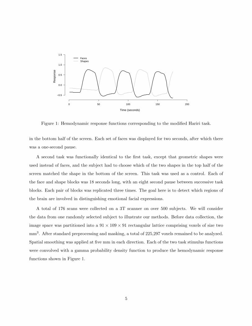
Figure 1: Hemodynamic response functions corresponding to the modified Hariri task.
in the bottom half of the screen. Each set of faces was displayed for two seconds, after which there
was a one-second pause.
A second task was functionally identical to the first task, except that geometric shapes were
used instead of faces, and the subject had to choose which of the two shapes in the top half of the
screen matched the shape in the bottom of the screen. This task was used as a control. Each of
the face and shape blocks was 18 seconds long, with an eight second pause between successive task
blocks. Each pair of blocks was replicated three times. The goal here is to detect which regions of
the brain are involved in distinguishing emotional facial expressions.
A total of 176 scans were collected on a 3T scanner on over 500 subjects. We will consider
the data from one randomly selected subject to illustrate our methods. Before data collection, the
image space was partitioned into a 91 × 109 × 91 rectangular lattice comprising voxels of size two
mm3. After standard preprocessing and masking, a total of 225,297 voxels remained to be analyzed.
Spatial smoothing was applied at five mm in each direction. Each of the two task stimulus functions
were convolved with a gamma probability density function to produce the hemodynamic response
functions shown in Figure 1.
5
2 Variable Selection in Bayesian Spatiotemporal Models
Detecting activation using (1) is equivalent to selecting the voxels with nonzero βv, and hence is a
variable selection problem. Bezener et al. (2015), Lee et al. (2014), Musgrove et al. (2015), Smith
and Fahrmeir (2007) and Smith et al. (2003) built on the approach of George and McCulloch (1993,
1997) to variable selection. However, Smith and Fahrmeir (2007) and Smith et al. (2003) ignored
temporal correlation, although they did incorporate spatial dependence in their models. Lee et al.
(2014) extended the approach of Smith and Fahrmeir (2007) and Smith et al. (2003) to include
both spatial and temporal dependence. All three of these papers rely on using a binary spatial
Ising prior to model the spatial dependence. While appealing from a modeling perspective, the
Ising prior results in substantial computational challenges that can be avoided with the approaches
described below. Both approaches are based on partitioning the image into three-dimensional
parcels and using a sparse spatial generalized linear mixed model (SGLMM). While there are many
commonalities between the two models, there are substantial differences between the models and
the required computation.
2.1 Bezener et al.’s (2015) Areal Model
Let Yv = (Yv,1, . . . , Yv,Tv)T be the time series of BOLD signal image intensities for voxel v = 1, . . . , N .
Suppose there are p experimental tasks or stimuli, and let Xv be a known Tv × p design matrix and
βv be a p× 1 vector. If Λv is a Tv × Tv positive definite matrix, assume
Yv = Xvβv + εv εv ∼ NTv(0, σ2vΛv) . (2)
The regression coefficients correspond to activation amplitudes, and detecting neuronal activation
is equivalent to detecting the nonzero βv,j . We will address this through the introduction of latent
variables. Let γv,j be binary random variables such that βv,j 6= 0 if γv,j = 1, and βv,j = 0 if γv,j = 0.
Let γv = (γv,1, γv,2, . . . , γv,p), so that βv(γv) is the vector of nonzero coefficients from βv, and Xv(γv)
is the corresponding design matrix. Model (2) can be expressed as
Yv = Xv(γv)βv(γv) + εv . (3)
6
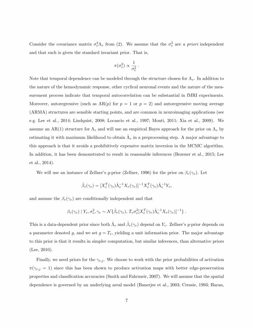
Consider the covariance matrix σ2vΛv from (2). We assume that the σ2v are a priori independent
and that each is given the standard invariant prior. That is,
π(σ2v) ∝1
σ2v.
Note that temporal dependence can be modeled through the structure chosen for Λv. In addition to
the nature of the hemodynamic response, other cyclical neuronal events and the nature of the mea-
surement process indicate that temporal autocorrelation can be substantial in fMRI experiments.
Moreover, autoregressive (such as AR(p) for p = 1 or p = 2) and autoregressive moving average
(ARMA) structures are sensible starting points, and are common in neuroimaging applications (see
e.g. Lee et al., 2014; Lindquist, 2008; Locascio et al., 1997; Monti, 2011; Xia et al., 2009). We
assume an AR(1) structure for Λv and will use an empirical Bayes approach for the prior on Λv by
estimating it with maximum likelihood to obtain Λv in a preprocessing step. A major advantage to
this approach is that it avoids a prohibitively expensive matrix inversion in the MCMC algorithm.
In addition, it has been demonstrated to result in reasonable inferences (Bezener et al., 2015; Lee
et al., 2014).
We will use an instance of Zellner’s g-prior (Zellner, 1996) for the prior on βv(γv). Let
βv(γv) = [XTv (γv)Λ
−1v Xv(γv)]
−1XTv (γv)Λ
−1v Yv,
and assume the βv(γv) are conditionally independent and that
βv(γv) | Yv, σ2v , γv ∼ N{βv(γv), Tvσ2v [XTv (γv)Λ
−1v Xv(γv)]
−1} .
This is a data-dependent prior since both Λv and βv(γv) depend on Yv. Zellner’s g-prior depends on
a parameter denoted g, and we set g = Tv, yielding a unit information prior. The major advantage
to this prior is that it results in simpler computation, but similar inferences, than alternative priors
(Lee, 2010).
Finally, we need priors for the γv,j . We choose to work with the prior probabilities of activation
π(γv,j = 1) since this has been shown to produce activation maps with better edge-preservation
properties and classification accuracies (Smith and Fahrmeir, 2007). We will assume that the spatial
dependence is governed by an underlying areal model (Banerjee et al., 2003; Cressie, 1993; Haran,
7
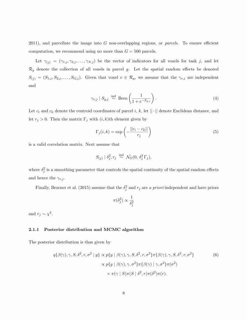
2011), and parcellate the image into G non-overlapping regions, or parcels. To ensure efficient
computation, we recommend using no more than G = 500 parcels.
Let γ(j) = (γ1,j , γ2,j , . . . , γN,j) be the vector of indicators for all voxels for task j, and let
Rg denote the collection of all voxels in parcel g. Let the spatial random effects be denoted
S(j) = (S1,j , S2,j , . . . , SG,j). Given that voxel v ∈ Rg, we assume that the γv,j are independent
and
γv,j | Sg,jind∼ Bern
(1
1 + e−Sg,j
). (4)
Let ci and ck denote the centroid coordinates of parcel i, k, let || · || denote Euclidean distance, and
let rj > 0. Then the matrix Γj with (i, k)th element given by
Γj(i, k) = exp
(−||ci − ck||
rj
)(5)
is a valid correlation matrix. Next assume that
S(j) | δ2j , rjind∼ NG(0, δ2j Γj),
where δ2j is a smoothing parameter that controls the spatial continuity of the spatial random effects
and hence the γv,j .
Finally, Bezener et al. (2015) assume that the δ2j and rj are a priori independent and have priors
π(δ2j ) ∝1
δ2j
and rj ∼ χ2.
2.1.1 Posterior distribution and MCMC algorithm
The posterior distribution is thus given by
q{β(γ), γ, S, δ2, r, σ2 | y} ∝ p{y | β(γ), γ, S, δ2, r, σ2}π{β(γ), γ, S, δ2, r, σ2} (6)
∝ p{y | β(γ), γ, σ2}π{β(γ) | γ, σ2}π(σ2)
× π(γ | S)π(S | δ2, r)π(δ2)π(r).
8

The dimension of the posterior in (6) is 2p(N + 1) + N + pG, which can be up to several millions
of variables. Our main goals are to determine which tasks and stimuli result in voxel activation as
well as to determine the amount of spatial dependence in the images. Thus, it is sufficient to work
with the marginal posterior
q(γ, S, r | y) =
∫q{β(γ), γ, S, δ2, r, σ2 | y} dβ(γ) dσ2 dδ2 , (7)
which is derived explicitly by Bezener et al. (2015).
The posterior in (7) is still analytically intractable, and so MCMC methods are required to
sample from it. Bezener et al. (2015) develop a component-wise MCMC approach based on the
posterior full conditional densities. That is,
q(γ | S, r, y) ∝ π(γ | S)N∏v=1
(1 + Tv)−qv/2K(γv)
−Tv/2
q(S | γ, r, y) ∝ π(γ | S)π(S | r)
q(r | S, γ, y) ∝ π(S | r)π(r) .
Schematically, one update of the MCMC algorithm looks like
(S, γ, r)→ (S′, γ, r)→ (S′, γ′, r)→ (S′, γ′, r′),
where each update is a Metropolis–Hastings step based on the relevant conditional density (for the
full details see Bezener et al. (2015)).
2.1.2 Starting Values
Selection of starting values for the MCMC simulation is an especially critical issue with a high-
dimensional posterior density. We suggest two strategies for choosing the MCMC starting values.
The first method is straightforward:
(1.) Set each γ(0)v,j = 0.
(2.) Initialize each spatial random effect as S(0)g,j ∼ N(0, τ2), where τ2 is small (e.g. τ2 = 0.001).
(3.) Set each spatial correlation parameter to its prior mean: r(0)j = E[π(rj)].
9
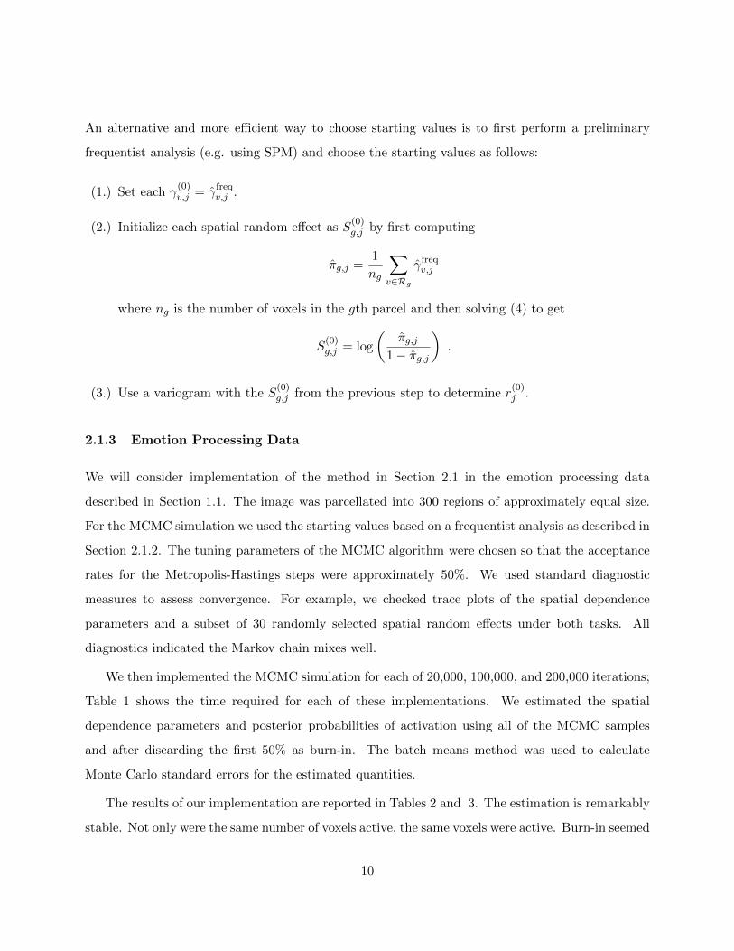
An alternative and more efficient way to choose starting values is to first perform a preliminary
frequentist analysis (e.g. using SPM) and choose the starting values as follows:
(1.) Set each γ(0)v,j = γfreqv,j .
(2.) Initialize each spatial random effect as S(0)g,j by first computing
πg,j =1
ng
∑v∈Rg
γfreqv,j
where ng is the number of voxels in the gth parcel and then solving (4) to get
S(0)g,j = log
(πg,j
1− πg,j
).
(3.) Use a variogram with the S(0)g,j from the previous step to determine r
(0)j .
2.1.3 Emotion Processing Data
We will consider implementation of the method in Section 2.1 in the emotion processing data
described in Section 1.1. The image was parcellated into 300 regions of approximately equal size.
For the MCMC simulation we used the starting values based on a frequentist analysis as described in
Section 2.1.2. The tuning parameters of the MCMC algorithm were chosen so that the acceptance
rates for the Metropolis-Hastings steps were approximately 50%. We used standard diagnostic
measures to assess convergence. For example, we checked trace plots of the spatial dependence
parameters and a subset of 30 randomly selected spatial random effects under both tasks. All
diagnostics indicated the Markov chain mixes well.
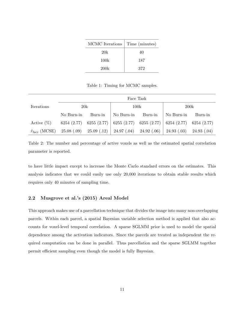
We then implemented the MCMC simulation for each of 20,000, 100,000, and 200,000 iterations;
Table 1 shows the time required for each of these implementations. We estimated the spatial
dependence parameters and posterior probabilities of activation using all of the MCMC samples
and after discarding the first 50% as burn-in. The batch means method was used to calculate
Monte Carlo standard errors for the estimated quantities.
The results of our implementation are reported in Tables 2 and 3. The estimation is remarkably
stable. Not only were the same number of voxels active, the same voxels were active. Burn-in seemed
10
MCMC Iterations Time (minutes)
20k 40
100k 187
200k 372
Table 1: Timing for MCMC samples.
Face Task
Iterations 20k 100k 200k
No Burn-in Burn-in No Burn-in Burn-in No Burn-in Burn-in
Active (%) 6254 (2.77) 6255 (2.77) 6255 (2.77) 6255 (2.77) 6254 (2.77) 6254 (2.77)
rface (MCSE) 25.08 (.09) 25.09 (.12) 24.97 (.04) 24.92 (.06) 24.93 (.03) 24.93 (.04)
Table 2: The number and percentage of active voxels as well as the estimated spatial correlation
parameter is reported.
to have little impact except to increase the Monte Carlo standard errors on the estimates. This
analysis indicates that we could easily use only 20,000 iterations to obtain stable results which
requires only 40 minutes of sampling time.
2.2 Musgrove et al.’s (2015) Areal Model
This approach makes use of a parcellation technique that divides the image into many non-overlapping
parcels. Within each parcel, a spatial Bayesian variable selection method is applied that also ac-
counts for voxel-level temporal correlation. A sparse SGLMM prior is used to model the spatial
dependence among the activation indicators. Since the parcels are treated as independent the re-
quired computation can be done in parallel. Thus parcellation and the sparse SGLMM together
permit efficient sampling even though the model is fully Bayesian.
11
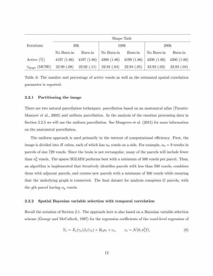
Shape Task
Iterations 20k 100k 200k
No Burn-in Burn-in No Burn-in Burn-in No Burn-in Burn-in
Active (%) 4197 (1.86) 4197 (1.86) 4200 (1.86) 4199 (1.86) 4200 (1.86) 4200 (1.86)
rshape (MCSE) 22.99 (.08) 22.92 (.11) 22.94 (.04) 22.94 (.05) 22.93 (.03) 22.93 (.04)
Table 3: The number and percentage of active voxels as well as the estimated spatial correlation
parameter is reported.
2.2.1 Partitioning the image
There are two natural parcellation techniques: parcellation based on an anatomical atlas (Tzourio-
Mazoyer et al., 2002) and uniform parcellation. In the analysis of the emotion processing data in
Section 2.2.5 we will use the uniform parcellation. See Musgrove et al. (2015) for more information
on the anatomical parcellation.
The uniform approach is used primarily in the interest of computational efficiency. First, the
image is divided into H cubes, each of which has n0 voxels on a side. For example, n0 = 9 results in
parcels of size 729 voxels. Since the brain is not rectangular, many of the parcels will include fewer
than n30 voxels. The sparse SGLMM performs best with a minimum of 500 voxels per parcel. Thus,
an algorithm is implemented that iteratively identifies parcels with less than 500 voxels, combines
them with adjacent parcels, and creates new parcels with a minimum of 500 voxels while ensuring
that the underlying graph is connected. The final dataset for analysis comprises G parcels, with
the gth parcel having ng voxels.
2.2.2 Spatial Bayesian variable selection with temporal correlation
Recall the notation of Section 2.1. The approach here is also based on a Bayesian variable selection
scheme (George and McCulloch, 1997) for the regression coefficients of the voxel-level regression of
Yv = Xv(γv)βv(γv) +Rvρv + εv, εv ∼ N (0, σ2vI), (8)
12
where Rv is a voxel-level lagged prediction matrix that is introduced to model temporal correlation.
Each of βv, γv, ρv, and σ2v is unknown. Variable selection is carried out in part by placing a spike-
and-slab mixture prior on the regression coefficients βv such that each βv,j , j = 1, . . . , p, is drawn
from a diffuse normal distribution (the slab) or a point mass at zero (the spike). This structure
reflects the prior belief that a coefficient is nonzero or zero, respectively. To facilitate MCMC
sampling, latent indicator variables γv = (γv,1, . . . , γv,p) are used such that the mixture prior for
each βvj has the form
π(βv,j | γv,j) = γv,jN(0, τ2j
)+ (1− γv,j)I0, (9)
where τ2j is an unknown stimulus-level variance and I0 denotes a point mass at zero. This prior
specification makes the natural assumption that the regression coefficients are a priori independent
conditional on the indicator variables (George and McCulloch, 1997). Spatial dependence between
voxels is modeled by placing a spatial prior on the indicator variables.
To account for the serial correlation present in the univariate voxel time series, an AR model
of order r is easily implemented and computationally efficient. Similar to Penny et al. (2003), the
matrix of lagged prediction errors, denoted Rv, is included in the regression model. The AR coeffi-
cients ρv,r = (ρv,1, . . . , ρv,r)′ are assumed a priori independent and normally distributed with mean
zero and known variance, which is typically taken to be “large.” To complete the voxel-level prior
specification, the error variance and stimulus-level variance are assumed a priori independent with
default priors π(σ2v)∝ 1/σ2v and π
(τ2j
)∝ 1/τ2j , respectively. In this way, regression coefficients
across voxels share a prior variance, resulting in additional smoothing beyond that induced by the
spatial prior.
2.2.3 Sparse SGLMM prior
The spatial prior is used to model the the voxel- and task-specific binary indicator variables γvj .
The chosen spatial prior is the sparse areal generalized linear mixed model (Hughes and Haran,
2013) and is used to account for spatial dependence for each of γj = (γ1,j , . . . , γng ,j)′, j = 1, . . . , p.
Specifically, the γj are conditionally independent Bernoulli random variables with a probit link
13
function such that
γv,j | ηv,jind∼ Bern{Φ(av,j + ηv,j)}
ηv,j = m′vδj + εv,j
εv,j ∼ N (0, 1) ,
(10)
where Φ(·) denotes the cumulative distribution function of a standard normal random variable, mv
is a vector of synthetic spatial predictors, δj = (δ1,j , . . . , δq,j) is a vector of spatial random effects,
av,j is an offset that controls the prior probability of activation, and ηv,j is an auxiliary variable
that is introduced to facilitate Gibbs sampling (Holmes and Held, 2006). Voxels are located at
the vertices of an underlying undirected graph, the structure of which reflects spatial adjacency
among voxels. For a partition of G parcels, with each parcel indexed by g, the graph is represented
using its parcel-level adjacency matrix A, which is ng × ng with entries given by diag(A) = 0 and
(A)u,v = I(u ∼ v). In the context of a two-dimensional analysis, a voxel neighborhood might
comprise the four nearest voxels. With three-dimensional fMRI data, a neighborhood contains the
26 nearest voxels.
The prior for the spatial random effects is
π(δj | κj)π(κj) = N{δj | 0, (κjM ′QM)−1
}× Gamma (κj | aκ , bκ) , (11)
where κj is a smoothing parameter; M is an ng× q matrix, the columns of which are the q principal
eigenvectors of A; and Q = D − A is the graph Laplacian, where D is the diagonal degree matrix.
Note that m′v is the vth row of M . The columns of M are multiresolutional spatial basis vectors
that are well suited for spatial smoothing and capture both the small-scale and large-scale spatial
variation typically exhibited by fMRI data (Woolrich et al., 2004). Sparsity is introduced by selecting
the columns of M corresponding to eigenvalues greater than 0.05. This choice permits appropriate
spatial smoothing while reducing the dimensionality considerably (typically, q < ng/2). The choice
of prior on the smoothing parameter κj follows Kelsall and Wakefield (1999) by using aκ = 1/2 and
bκ = 2000, which does not lead to artifactual spatial structure in the posterior.
14
2.2.4 Posterior computation and inference
Denote the voxel-level parameters as θv = (β′v, γ′v, ρ′v, σ
2v , )′, and the parcel-level parameters as
Θg = (δ′, κ′, (τ2)′)′. Within the gth parcel (having ng voxels), the prior distribution is
π(θv,Θg) =
ng∏v=1
π(ρv)π(σ2v)π(βv | γv)p∏j=1
π(γj | δj)π(δj | κj)π(κj)π(τ2j ),
which implies that the between-voxel and between-task parameters are conditionally independent
a priori. The posterior distribution is obtained in the usual way by combining priors and the
likelihood.
To obtain updates for each γv,j , a voxel-level likelihood is used where βv,j has been integrated
out analytically. For Wv,t,(j) = Yv,t −∑p
l 6=j Xt,lβv,l, let W ∗v,t,(j) = Wv,t,(j) −∑r
k=1 ρv,kWv,t−k,(j), and
let X∗t,j = Xt,j −∑r
k=1 ρv,kXt−k,j . Then, conditional on γv,j , the likelihood can be written as a
mixture with two components:
L1 = τ−1j exp
{− 1
2σ2v
T∑t=1
(W ∗v,t,(j) −X
∗t,jβv,j
)2− 1
2τ2jβ2v,j
}
and
L0 = exp
{− 1
2σ2v
T∑t=1
W ∗2v,t,(j)
},
where L1 is the voxel-level likelihood when γv,j = 1, and L0 is the likelihood when γv,j = 0.
Integrating βv,j out of L1, it is straightforward to show that
L1 = τ−1j σ∗−1v,j exp
− 1
2σ2v
T∑t=1
W ∗2v,t,(j) +1
2σ∗2v,j
(1
σ2v
T∑t=1
W ∗v,t,(j)X∗t,j
)2 ,
where σ∗2v,j = σ−2v∑T
t=1X∗2t,j+τ
−2j . The posterior probability that γv,j = 1 is q (γv,j = 1 | Yv, ·) = (1 + P)−1,
where
P =L0
L1
q (γv,j = 0 | ηj)q (γv,j = 1 | ηj)
.
Conditional on γv,j = 0, set βv,j = 0. Otherwise, βv,j is updated from its full conditional
distribution. Writing W ∗v,t,(j) = X∗t,jβv,j + εv,t, and using the fact that the error term is normally
distributed, each βv,j has a normal prior distribution. Conditional on γv,j = 1, the posterior
15
distribution of βv,j is N (βv,j , τ2v,j), where
βv,j = τ2v,j
T∑t=1
W ∗v,t,(j)X∗t,j and τ2v,j =
(T∑t=1
X∗2t,j + σ2v/τ2j
)−1.
Posterior sampling of each of ηj = (η1,j , . . . , ηng ,j)′, δj , and κj uses probit regression with auxil-
iary variables, conditional on γv,j only (Holmes and Held, 2006). The full conditional distributions
are given in (Musgrove et al., 2015).
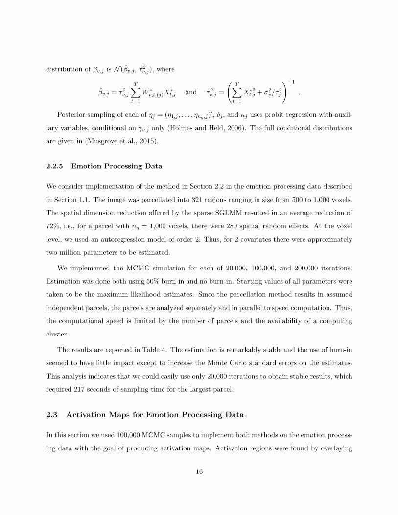
2.2.5 Emotion Processing Data
We consider implementation of the method in Section 2.2 in the emotion processing data described
in Section 1.1. The image was parcellated into 321 regions ranging in size from 500 to 1,000 voxels.
The spatial dimension reduction offered by the sparse SGLMM resulted in an average reduction of
72%, i.e., for a parcel with ng = 1,000 voxels, there were 280 spatial random effects. At the voxel
level, we used an autoregression model of order 2. Thus, for 2 covariates there were approximately
two million parameters to be estimated.
We implemented the MCMC simulation for each of 20,000, 100,000, and 200,000 iterations.
Estimation was done both using 50% burn-in and no burn-in. Starting values of all parameters were
taken to be the maximum likelihood estimates. Since the parcellation method results in assumed
independent parcels, the parcels are analyzed separately and in parallel to speed computation. Thus,
the computational speed is limited by the number of parcels and the availability of a computing
cluster.
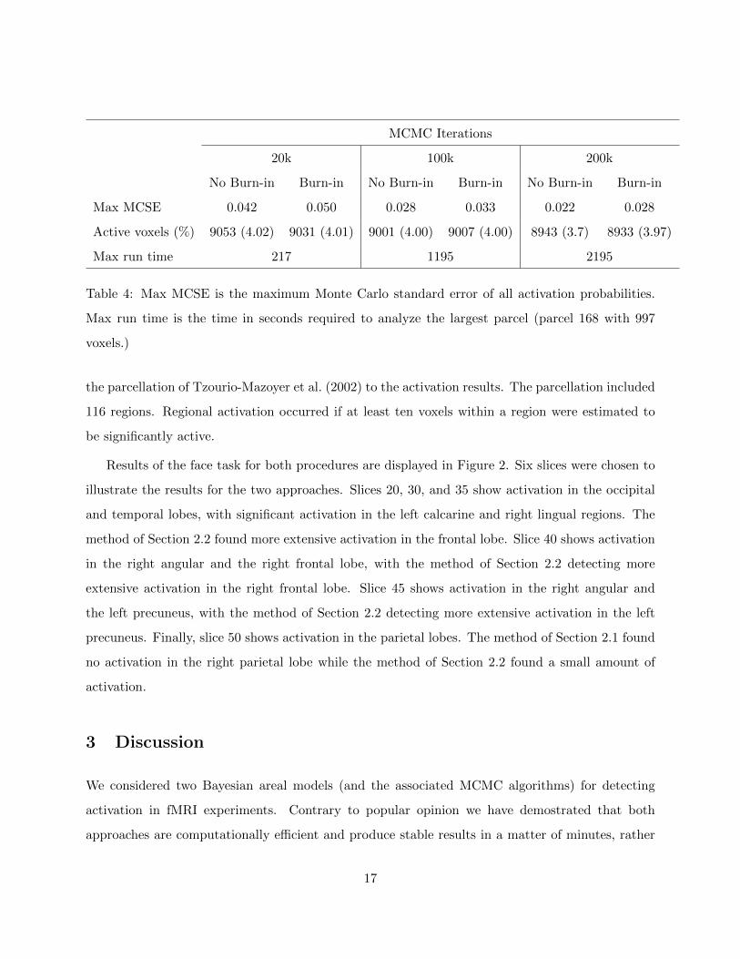
The results are reported in Table 4. The estimation is remarkably stable and the use of burn-in
seemed to have little impact except to increase the Monte Carlo standard errors on the estimates.
This analysis indicates that we could easily use only 20,000 iterations to obtain stable results, which
required 217 seconds of sampling time for the largest parcel.
2.3 Activation Maps for Emotion Processing Data
In this section we used 100,000 MCMC samples to implement both methods on the emotion process-
ing data with the goal of producing activation maps. Activation regions were found by overlaying
16
MCMC Iterations
20k 100k 200k
No Burn-in Burn-in No Burn-in Burn-in No Burn-in Burn-in
Max MCSE 0.042 0.050 0.028 0.033 0.022 0.028
Active voxels (%) 9053 (4.02) 9031 (4.01) 9001 (4.00) 9007 (4.00) 8943 (3.7) 8933 (3.97)
Max run time 217 1195 2195
Table 4: Max MCSE is the maximum Monte Carlo standard error of all activation probabilities.
Max run time is the time in seconds required to analyze the largest parcel (parcel 168 with 997
voxels.)
the parcellation of Tzourio-Mazoyer et al. (2002) to the activation results. The parcellation included
116 regions. Regional activation occurred if at least ten voxels within a region were estimated to
be significantly active.
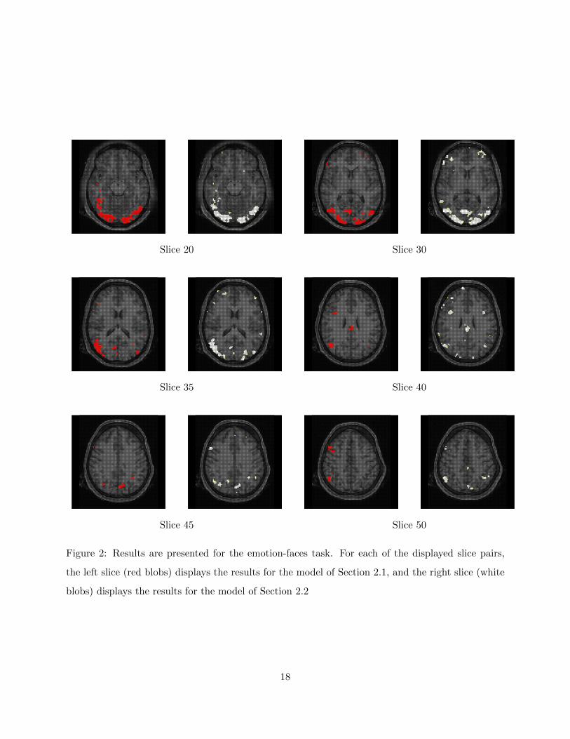
Results of the face task for both procedures are displayed in Figure 2. Six slices were chosen to
illustrate the results for the two approaches. Slices 20, 30, and 35 show activation in the occipital
and temporal lobes, with significant activation in the left calcarine and right lingual regions. The
method of Section 2.2 found more extensive activation in the frontal lobe. Slice 40 shows activation
in the right angular and the right frontal lobe, with the method of Section 2.2 detecting more
extensive activation in the right frontal lobe. Slice 45 shows activation in the right angular and
the left precuneus, with the method of Section 2.2 detecting more extensive activation in the left
precuneus. Finally, slice 50 shows activation in the parietal lobes. The method of Section 2.1 found
no activation in the right parietal lobe while the method of Section 2.2 found a small amount of
activation.
3 Discussion
We considered two Bayesian areal models (and the associated MCMC algorithms) for detecting
activation in fMRI experiments. Contrary to popular opinion we have demostrated that both
approaches are computationally efficient and produce stable results in a matter of minutes, rather
17
Slice 20 Slice 30
Slice 35 Slice 40
Slice 45 Slice 50
Figure 2: Results are presented for the emotion-faces task. For each of the displayed slice pairs,
the left slice (red blobs) displays the results for the model of Section 2.1, and the right slice (white
blobs) displays the results for the model of Section 2.2
18
than hours or days. Both methods are based on parcellations. In Section 2.1 the parcellations are
not assumed independent, while in Section 2.2 they are. The advantage of assuming independence is
that the computation may then be parallelized. The disadvantage is that it is a somewhat awkward
assumption that seems to have little relevance to the underlying science. On the other hand the
computation required in Section 2.1 is not parallelizeable and hence takes longer. In the emotion
processing data example we see that both approaches yield similar results, although the approach
of Section 2.2 yields more active voxels than does the approach of Section 2.1.
Acknowledgments
Data were provided by the Human Connectome Project, WU-Minn Consortium (Principal Investi-
gators: David Van Essen and Kamil Ugurbil; 1U54MH091657) funded by the 16 NIH Institutes and
Centers that support the NIH Blueprint for Neuroscience Research; and by the McDonnell Center
for Systems Neuroscience at Washington University.
References
Aguirre, G. K., Zarahan, E., and D’Esposito, M. (1998). The variability of human, BOLD hemo-
dynamic repsonses. NeuroImage, 8:360–369.
Aguirre, G. K., Zarahn, E., and D’Esposito, M. (1997). Empirical analyses of BOLD fMRI statis-
tics. II. Spatially smoothed data collected under null-hypothesis and experimental conditions.
NeuroImage, 5:199–212.
Banerjee, S., Carlin, B. P., and Gelfand, A. E. (2003). Hierarchical Modeling and Analysis for
Spatial Data. Chapman and Hall/CRC, New York, 1st edition.
Bezener, M., Hughes, J., and Jones, G. L. (2015). Bayesian spatiotemporal modeling using hierar-
chical spatial priors with applications to functional magnetic resonance imaging. Preprint.
Bowman, F. D. (2014). Brain imaging analysis. Annual Review of Statistics and Its Application,
1:61–85.
19
Cressie, N. A. (1993). Statistics for Spatial Data. Wiley Interscience, New York, Revised edition.
Essen, D. C. V., Smith, S. M., Barch, D. M., Behrens, T. E., Yavoub, E., and Ugurbil, K. (2013).
The WU-Minn Human Connectome Project: An overview. Neuroimage, pages 62–79.
Friston, K. J., Ashburner, J. T., Kiebel, S. J., Nichols, T. E., and Penny, W. D. (2007). Statistical
Parametric Mapping: The Analysis of Functional Brain Images. Academic Press, London.
Friston, K. J., Holmes, A., Worsley, K. J., Polin, J. B., Frith, C., and Frackowik, R. (1995).
Statistical parametric maps in functional imaging: A general linear approach. Human Brain
Mapping, 2:189–210.
Friston, K. J., Worsley, K., Frackowiak, R., Mazziotta, J., and Evans, A. (1994). Assessing the
significance of focal activations using their spatial extent. Human Brain Mapping, 1:210–220.
Genovese, C. R. (2000). A Bayesian time-course model for functional magnetic resonance imaging
data. Journal of the American Statistical Association, 95(451):691–703.
George, E. I. and McCulloch, R. E. (1993). Variable selection via Gibbs sampling. Journal of the
American Statistical Association, 88(423):881–889.
George, E. I. and McCulloch, R. E. (1997). Approaches for Bayesian variable selection. Statistica
Sinica, 7:339–373.
Haran, M. (2011). Gaussian random field models for spatial data. In Brooks, S. P., Gelman, A. E.,
Jones, G. L., and Meng, X. L., editors, Handbook of Markov Chain Monte Carlo, pages 449–478.
Chapman and Hall/CRC, London.
Hariri, A. R., Mattay, V. S., Tessitore, A., Kolachana, B., Fera, F., Goldman, D., Egan, M. F., and
Weinberger, D. R. (2002). Serotonin transporter genetic variation and the response of human
amygdala. Science, 297:400–4003.
Hensen, R. and Friston, K. (2007). Convolution models for fMRI. In Statistical Parametric Mapping:
The Analysis of Functional Brain Images. Academic Press.
20
Holmes, A. P., Blair, R. C., Watson, J. D., and Ford, I. (1996). Nonparametric analysis of statistic
images from functional mapping experiments. Journal of Cerebral Blood Flow & Metabolism,
16:7–22.
Holmes, C. C. and Held, L. (2006). Bayesian auxiliary variable models for binary and multinomial
regression. Bayesian Analysis, 1(1):145–168.
Huettel, S. A., Somng, A. W., and McCarthy, G. (2009). Functional Magnetic Resonance Imaging.
Sinauer Associates, Sunderland, MA.
Hughes, J. and Haran, M. (2013). Dimension Reduction and Alleviation of Confounding for Spatial
Generalized Linear Mixed Models. Journal of the Royal Statistical Society: Series B (Statistical
Methodology), 75(1):139–159.
Kaushik, K., Karesh, K., and Suresha, D. (2013). Segmentation of the white matter from the
brain fMRI images. International Journal of Advanced Research in Computer Engineering and
Technology, 2:1314–1317.
Kelsall, J. and Wakefield, J. (1999). Discussion of “Bayesian Models for Spatially Correlated Disease
and Exposure Data”, by Best et al. In Berger, J., Bernardo, J., Dawid, A., and Smith, A., editors,
Bayesian Statistics 6. Oxford University Press.
Lazar, N. A. (2008). The Statistical Analysis of fMRI Data. Springer, New York.
Lee, K.-J. (2010). Computational issues in using Bayesian hieratchical methods for the spatial
modeling of fMRI data. PhD thesis, University of Minnesota, School of Statistics.
Lee, K.-J., Jones, G. L., Caffo, B. S., and Bassett, S. S. (2014). Spatial Bayesian variable selection
models on functional magnetic resonance imaging time-series data. Bayesian Analysis, 9:699–732.
Lindquist, M. A. (2008). The statistical analysis of fMRI data. Statistical Science, 23:439–464.
Locascio, J., Jennings, P. J., Moore, C. I., and Corkin, S. (1997). Time series analysis in the time
domain and resampling methods for studies of functional magnetic brain imaging. Human Brain
Mapping, pages 168–193.
21
Makni, S., Idier, J., Vincent, T., Thirion, B., Dehaene-Lambertz, G., and Ciuciu, P. (2008). A fully
Bayesian approach to the parcel-based detection-estimation of brain activity in fMRI. NeuroIm-
age, 41:941–969.
Mikl, M., Marecek, R., Hlustık, P., Pavlicova, M., Drastich, A., Chlebus, P., Brazdil, M., and
Krupa, P. (2008). Effects of spatial smoothing on fMRI group inferences. Magnetic Resonance
Imaging, 26:490–503.
Monti, M. M. (2011). Statistical analysis of fMRI time-series: A critical review of the GLM approach.
Frontiers in Human Neuroscience, 5.
Musgrove, D. R., Hughes, J., and Eberly, L. E. (2015). Fast, fully Bayesian spatiotemporal inference
of fMRI data. Preprint.
Penny, W., Kiebel, S., and Friston, K. (2003). Variational Bayesian inference for fMRI time series.
NeuroImage, 19:727–741.
Smith, M. and Fahrmeir, L. (2007). Spatial Bayesian variable selection with application to functional
magnetic resonance imaging. Journal of the American Statistical Association, 102(478):417–431.
Smith, M., Putz, B., Auer, D., and Fahrmeir, L. (2003). Assessing brain activity through spatial
Bayesian variable selection. NeuroImage, 20.
Triantafyllou, C., Hoge, R., and Wald, L. (2006). Effect of spatial smoothing on physiological noise
in high-resolution fMRI. NeuroImage, 32:551–557.
Tzourio-Mazoyer, N., Landeau, B., Papathanassiou, D., Crivello, F., Etard, O., Delcroix, N., Ma-
zoyer, B., and Joliot, M. (2002). Automated anatomical labeling of activations in spm using a
macroscopic anatomical parcellation of the mni mri single-subject brain. Neuroimage, 15(1):273–
289.
Woolrich, M. W., Jenkinson, M., Brady, J. M., and Smith, S. M. (2004). Fully Bayesian spatio-
temporal modeling of fMRI data. IEEE Transactions on Medical Imaging, 23:213–231.
22
Worsley, K., Marrett, S., Neelin, P., and Evans, A. (1992). A three-dimensional statistical analysis
for CBF activation studies in human brain. Journal of Cerebral Blood Flow and Metabolism,
12:900–918.
Xia, J., Liang, F., and Wang, Y. M. (2009). fMRI analysis through Bayesian variable selection with
a spatial prior. IEEE Int. Symp. on Biomedical Imaging (ISBI), pages 714–717.
Zellner, A. (1996). On assessing prior distributions and Bayesian regression analysis with g-prior
distributions. In Bayesian Inference and Decision Techniques: Essays in Honor of Brunode
Finetti North-Holland/Elsevier, pages 233–243.
Zhang, L., Guindani, M., and Vannucci, M. (2015). Bayesian models for functional magnetic
resonance imaging data analysis. WIREs Computational Statistics, 7:21–41.
23