B

R

d1aaaHimptiit

E

w

©

GEOPHYSICS, VOL. 73, NO. 5 �SEPTEMBER-OCTOBER 2008�; P. S207–S217, 11 FIGS.10.1190/1.2969776

eamlet migration using local cosine basis

u-Shan Wu1, Yongzhong Wang2, and Mingqiu Luo3

fqwwrtMcbwrp�cc

ABSTRACT

We have developed the theoretical foundation and technicaldetails of a migration method using a local-cosine-bases �LCB�beamlet propagator. A beamlet propagator for heterogeneousmedia based on local perturbation theory is derived, and a fastimplementation method is constructed. The use of local back-ground velocities and local perturbations results in a two-scaledecomposition of beamlet propagators: a background propagatorfor large-scale structures and a local phase-screen correction forsmall-scale local perturbations. Because of its locally adaptivenature, the beamlet propagator can handle strong lateral velocityvariations with improved accuracy. For high-efficiency migra-tion, we use a table-driven method and apply some techniques ofsparse matrix operations. Compared with the Fourier finite-dif-

bs

sw�ppmfgiagfi

receiveetary Ph

esently

luo@sc

S207

erence and generalized screen propagator methods, the imageuality and computational efficiency are similar. In some cases,e see fewer migration artifacts around and inside salt bodiesith our method. We attribute this to the better high-angle accu-

acy of beamlet propagators in strong-contrast media. Numericalests using synthetic data sets of the SEG-EAGE 2D salt model,

armousi model, and Sigsbee 2Amodel demonstrate its high ac-uracy and reasonable efficiency.Another special feature of LCBeamlet migration is the availability of information in the localavenumber domain during migration, which can be used to cor-

ect acquisition aperture effect and for other processing. Com-ared to beamlet migration using the Gabor-Daubechies frameGDF� propagator, LCB migration is much more efficient be-ause LCB is an orthonormal basis, whereas GDF has redundan-y �usually greater than two� in the decomposition.

INTRODUCTION

Wave-equation-based migration methods implemented in dualomains, i.e., space and wavenumber �Ristow and Rühl, 1994; Wu,994; Wu and Xie, 1994; Xie and Wu, 1998, 1999, 2005; Huang etl., 1999a, 1999b; Jin et al., 1999, 2002; de Hoop et al., 2000; Huangnd Fehler, 2000�, can handle lateral velocity variations with reason-ble accuracy and efficiency using the fast Fourier transform �FFT�.owever, the treatment of strong lateral velocity variations, such as

n subsalt imaging, is still a great challenge. In the dual-domainethods, at each depth the velocity profile of the medium is decom-

osed into a global background �reference� velocity and global per-urbations. Propagation in the homogeneous reference medium ismplemented in the wavenumber domain by phase shift, whereas thenteraction of the wavefield with the perturbations is performed inhe space domain. For strong-contrast media, the perturbations can

Manuscript received by the Editor 17 September 2007; revised manuscript1University of California, Santa Cruz, Institute of Geophysics and Plan

-mail: wrs@pmc.ucsc.edu.2 Formerly Geophysical Development Corp., Houston, Texas, U.S.A.; pr

ang@geokinetics.com.3Screen Imaging Tech., Inc. �SITI�, Sugar Land, Texas, U.S.A. E-mail: mq2008 Society of Exploration Geophysicists.All rights reserved.

e very large. The propagation of high-angle waves �steep events� inuch media remains a tough problem.

To improve the accuracy of high-angle waves propagating introng-contrast media, some research has been done to localize theavefield in both the space and wavenumber domains. Steinberg

1993� and Steinberg and Birman �1995� derive the phase-spaceropagators using the windowed Fourier transform �WFT� and aerturbation approach. The localized propagators are controlledainly by the local properties of the heterogeneous medium; there-

ore, they tend to make better approximations than the global propa-ators. However, decomposition and reconstruction using WFT andnverse WFT are very expensive; hence, the method is difficult todopt in practical use. Additionally, the method is formulated with alobal perturbation to the partial-differential wave equation; there-ore, large perturbations in strong-contrast media are still handlednaccurately, even for localized waves.

d 13 February 2008; published online 26 September 2008.ysics, Modeling and Imaging Laboratory, Santa Cruz, California, U.S.A.

Geokinetics Processing, Inc., Houston, Texas, U.S.A. E-mail: yongzhong.

reenimaging.com.

Jglesct

aMt2b2waglgb

ssoabpvtt

mfstAwbwis

�sipt

WHDtpltw

wc�

B

wa

w

Tp

T

e

m

F

S208 Wu et al.

The windowed screen method was introduced �Wu and Jin, 1997;in and Wu, 1998, 1999� to circumvent the difficulty imposed by thelobal perturbation method. In this method, a local background ve-ocity and local perturbations are introduced through the WFT. How-ver, because the perfect WFT reconstruction is formidably expen-ive, the method relies on broadly overlapped windows and empiri-al interpolations, generally making it applicable only when few dis-inct material boundaries exist.

A beamlet migration approach based on local reference velocitiesnd local perturbation theory has been proposed �Wu et al., 2000�.igration methods based on this theory have been developed using

he Gabor-Daubechies frame �GDF� �Wu and Chen, 2001, 2002a,002b, 2006; Chen and Wu, 2002; Chen et al., 2006� and local cosineases �LCB� �Wang and Wu, 2002; Luo and Wu, 2003; Wang et al.,003, 2005; Wu et al., 2003; Luo et al., 2004�. In these methods, theavefields are localized spatially with local windows and direction-

lly with local wavenumbers. The wavefield at each depth is propa-ated with beamlet propagators �sparse propagator matrices�, fol-owed by local perturbation corrections. These methods can provideood imaging results when compared to traditional wave-equation-ased methods.

We first introduce the LCB and wavefield decomposition/recon-truction with it. Then we describe the theory and method of con-tructing the propagator matrix in the LCB beamlet domain, basedn local perturbation theory. The beamlet propagator is composed ofbackground propagator that propagates beamlets in large-scale

ackground media and a perturbation operator that performs localerturbation corrections accounting for small-scale lateral velocityariations. To calculate the background propagator, we adopt twoypes of approximations: the local homogeneous approximation andhe average slowness approximation.

In this paper, we concentrate on the 2D implementation of theethod and develop a fast algorithm using the fast local cosine trans-

orm, a sparse matrix calculation, and a table-driven scheme to con-truct the propagator matrix. In the numerical examples, we applyhe method to poststack depth migration of the SEG/EAGE 2D A-� salt model and prestack migrations of the Marmousi model asell as the 2D Smaart JV Sigsbee2A model. We find that the LCBeamlet propagator can handle strong lateral velocity variationsith improved accuracy. The efficiency of LCB beamlet migration

s comparable to Fourier finite-difference �FFD� and generalizedcreen propagator �GSP� one-way wave migration.

LOCAL COSINE BASES

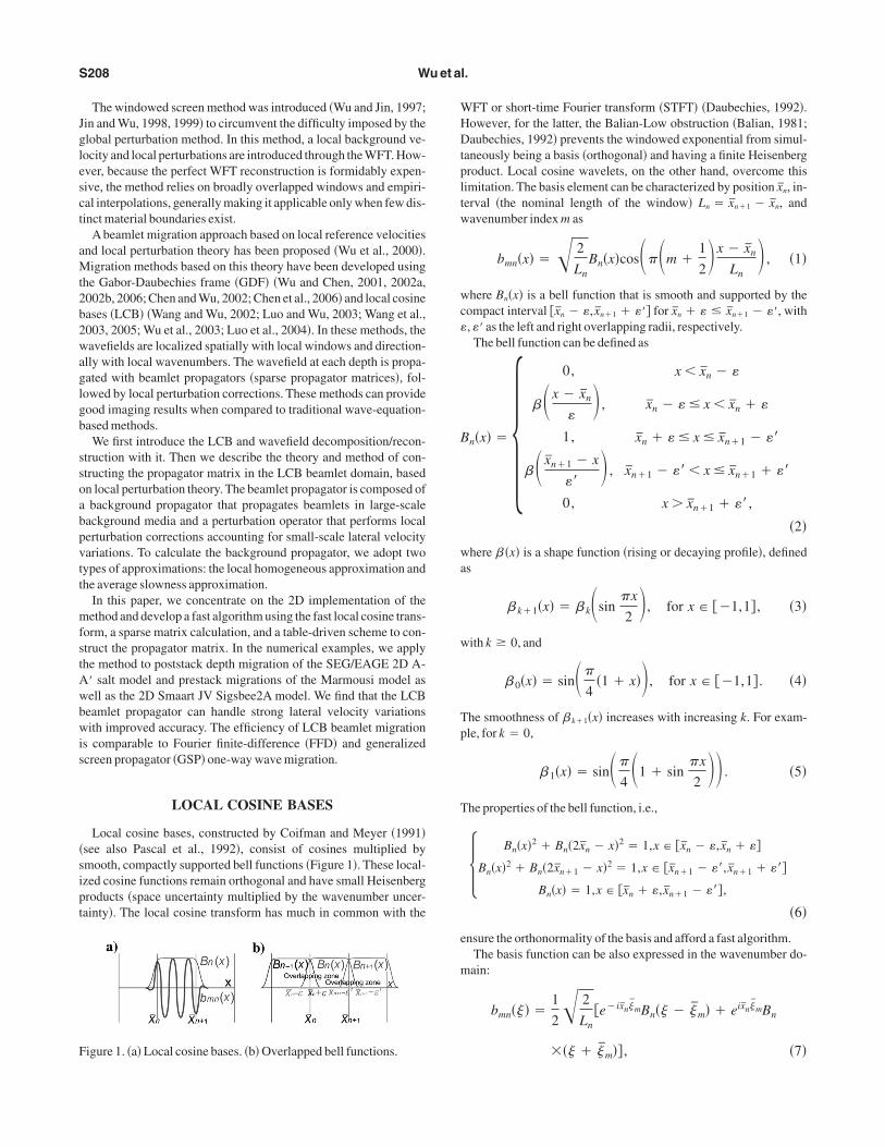
Local cosine bases, constructed by Coifman and Meyer �1991�see also Pascal et al., 1992�, consist of cosines multiplied bymooth, compactly supported bell functions �Figure 1�. These local-zed cosine functions remain orthogonal and have small Heisenbergroducts �space uncertainty multiplied by the wavenumber uncer-ainty�. The local cosine transform has much in common with the

igure 1. �a� Local cosine bases. �b� Overlapped bell functions.

FT or short-time Fourier transform �STFT� �Daubechies, 1992�.owever, for the latter, the Balian-Low obstruction �Balian, 1981;aubechies, 1992� prevents the windowed exponential from simul-

aneously being a basis �orthogonal� and having a finite Heisenbergroduct. Local cosine wavelets, on the other hand, overcome thisimitation. The basis element can be characterized by position xn, in-erval �the nominal length of the window� Ln � xn�1 � xn, andavenumber index m as

bmn�x� �� 2

LnBn�x�cos���m �

1

2� x � xn

Ln� , �1�

here Bn�x� is a bell function that is smooth and supported by theompact interval �xn � �, xn�1 � ��� for xn � � � xn�1 � ��, with, �� as the left and right overlapping radii, respectively.The bell function can be defined as

n�x� ��0, x � xn � �

�� x � xn

�� , xn � � � x � xn � �

1, xn � � � x � xn�1 � ��

�� xn�1 � x

��� , xn�1 � �� � x � xn�1 � ��

0, x � xn�1 � ��,

�2�

here � �x� is a shape function �rising or decaying profile�, defineds

� k�1�x� � � k�sin�x

2�, for x � ��1,1� , �3�

ith k � 0, and

� 0�x� � sin��

4�1 � x��, for x � ��1,1� . �4�

he smoothness of � k�1�x� increases with increasing k. For exam-le, for k � 0,

� 1�x� � sin��

4�1 � sin

�x

2�� . �5�

he properties of the bell function, i.e.,

� Bn�x�2 � Bn�2xn � x�2 � 1,x � �xn � �, xn � ��

Bn�x�2 � Bn�2xn�1 � x�2 � 1,x � �xn�1 � ��, xn�1 � ���

Bn�x� � 1,x � �xn � �, xn�1 � ��� ,�6�

nsure the orthonormality of the basis and afford a fast algorithm.The basis function can be also expressed in the wavenumber do-ain:

bmn�� � �1

2� 2

Ln�e�ixn� mBn�� � � m� � eixn� mBn

�� � � �� , �7�

m

wB

ivctft�Ift

wptsslbncipt

W

e

wfir

w

wntawpc

t

is1dsaw

wfi

P

te

Iifieg

FSbdb

Local cosine beamlet migration S209

here Bn�� � is the Fourier transform of the bell �window� function

n�x� and � m � ���m �12��/Ln.

A local cosine transform �LCT� �and inverse transform� can bemplemented by fast algorithms, such as the one introduced by Mal-ar �1992� �see also Mallat, 1999�. The fast LCT uses a folding pro-edure to make the windowed section into a periodic function andhen implements the local projection by fast discrete cosine trans-orm �DCT�. The fast algorithm has an order of O�Nxlog2Nw� compu-ations, where Nx is the number of samples along the transform linein the x-direction� and Nw is the window length in sampling points.n the case of large Nx �long lateral extent�, the LCT is theoreticallyaster than the FFT, which has an order of O�Nxlog2Nx� computa-ions.Appendix A gives more details about the fast LCT.

ONE-WAY WAVE PROPAGATIONIN THE BEAMLET DOMAIN

The wavefield can be decomposed into beamlets, the elementaryaves in the beamlet domain, through the LCT. One-way waveropagation also can be formulated in the beamlet domain, leadingo wave propagation in the beamlet domain. In general, especially introngly heterogeneous media, the beamlets will be distorted andcattered after propagation and therefore will not remain individual-y as elementary waves. To express the propagated wavefield into theeamlet basis, we must redecompose the distorted beamlets into aew set of beamlets, i.e., a beamlet is coupled into other beamlets be-ause of propagation and scattering. Only forward propagation ismportant for the application of beamlet propagation to the imagingroblem; backscattering is neglected. Therefore, we formulate onlyhe one-way wave propagation in the beamlet domain.

avefield decomposition

Generally in the frequency-space �f-x� domain, the scalar wavequation can be written as

� x2 � � z

2 �2

V2�x,z��u�x,z,� � 0, �8�

here denotes frequency, V�x,z� is velocity, and u�x,z,� standsor the frequency-domain wavefield. For simplicity, u�x,z� is usednstead of u�x,z,� to denote the frequency-domain wavefield in theest of the paper.

The wavefield at depth z can be decomposed into beamlets withindows along the x-axis:

u�x,z� � �n

�m

u�x,z�,bmn�x��bmn�x�

� �n

�m

u�xn, � m;z�bmn�x� , �9�

here bmn�x� are the decomposition beamlets. Because of the ortho-ormality of the LCB, bmn�x� are also the reconstruction beamlets;he basis function is defined by equation 1. In equation 9, u�xn, � m;z�re the coefficients of the decomposition beamlets located at spaceindow xn and wavenumber window � m, and �,� stands for innerroduct as u�x,z�,bmn�x�� � �u�x,z�b

mn* �x�dx, where * denotes the

omplex conjugate. Note that bmn* �x� � bmn�x� because bmn�x� is real.

If the space and wavenumber windows are partitioned uniformly,hen x � n�x, � � m�� , and �x, �� , are the sampling intervals

n m

n the x-axis and wavenumber � -axis, respectively. If the decompo-ition beamlets are not orthogonal, such as the frames �Daubechies,992�, the reconstruction beamlets have to be the dual atoms of theecomposition atoms. For an application of GDF beamlet decompo-ition and propagation, see Wu et al. �2000�, Wu and Chen �2002b�,nd Chen et al. �2006�. Figure 2a illustrates the decomposition of theavefield into beamlets.Note that the local cosines are real functions. The inner product

u,bmn� implies

u,bmn� � ur,bmn� � i ui,bmn� , �10�

here ur and ui are the real and imaginary parts of the complex wave-eld, respectively.

ropagation in the beamlet domain

Substituting the wavefield decomposition equation 9 into equa-ion 8, the beamlets will also propagate obeying the scalar wavequation

�n

�m

u�xn, � m;z�� x2 � � z

2 �2

V2�x,z��bmn�x� � 0.

�11�

n equation 11, u�xn, � m;z� is a set of coefficients with z as the label-ng parameter, not a variable. The propagation effect of the wave-eld is now included in the evolution of beamlets. For a local beamvolution problem, invoking the one-way wave approximation �ne-lecting interactions between the forward-scattered and backscat-

igure 2. One-way wave propagation in the beamlet domain. �a�pace-domain wavefield is decomposed into the summation ofeamlets. �b� Wave propagation in the beamlet domain. �c� Space-omain wavefield at depth z � �z is reconstructed from the neweamlets.

tb

Hh

af

T

T

HPub

W

soc

Hiee

ttHanw

epgiwfsvl

L

Vcalfiew�a

wpatH

w

iw

i

sstc

nbts

S210 Wu et al.

ered waves�, we can write a formal solution for the evolution ofeamlets:

amn�x� � e�iAn�zbmn�x� . �12�

ere, amn is a function evolved from a beamlet bmn propagating in theeterogeneous medium and An is the square-root operator,

An ��� x2 �

2

V2�x,z�. �13�

As mentioned, amn is no longer a beamlet because of the distortionfter propagation. Decomposing amn with the same beamlet basesunctions

amn�x� � �l

�j

amn,bjl�bjl�x� . �14�

he propagator matrix P in the beamlet domain is

Pjl,mn � P�xl, � j; xn, � m� � amn�x�,bjl�x�� . �15�

he beamlet-domain wavefield at depth z � �z can be obtained as

u�xl, � j;z � �z� � �n

�m

P�xl, � j; xn, � m�u�xn, � m;z�

� �n

�m

Pjl,mnu�xn, � m;z� . �16�

ere, Pjl,mn are the matrix elements of the beamlet propagator matrix, which governs the beamlet propagation and cross-coupling. Fig-re 2b illustrates conceptually the propagation and cross-coupling ofeamlets.

avefield reconstruction

We limit the beamlet decomposition to the use of orthogonal baseso the reconstruction atoms are the same as the decomposition at-ms.As shown in Figure 2c, the wavefield at depth z � �z can be re-onstructed from the beamlet-domain wavefield through

u�x,z � �z� � �n

�m

u�xn, � m;z�amn�x�

� �l

�j

u�xl, � j;z � �z�bjl�x� . �17�

BEAMLET PROPAGATOR WITH LOCALPERTURBATION APPROXIMATION

Equation 15 formally defines the beamlet propagator matrix.owever, calculation of the beamlet propagator is quite complicated

n generally heterogeneous media. The evolution of beamlets is gov-rned by the operator equation 12, which involves a square-root op-rator. No exact solution is available for a general problem.

Various approximations are invoked to make the calculation prac-ical. High-frequency asymptotic approximations can be applied tohe evolution of beamlets in smoothly varying media �Foster anduang, 1991; Steinberg, 1993�. However, the accuracy of the

symptotic solution becomes unacceptable for strongly heteroge-eous media. On the other hand, exploring the efficiency of fastavelet transforms and the sparseness of the propagator matrix, Wu

t al. �2000� apply a local perturbation approximation to the beamletropagator, resulting in a split-step implementation of wave propa-ation in the beamlet domain. Because no high-frequency asymptot-cs are involved, the local perturbation approach can keep all of theave phenomena of forward propagation, such as diffraction, inter-

erence, and scattering and cross-coupling between beamlets, in theimulation. We apply the local perturbation approximation and de-elop specific techniques of fast implementation to the LCB beam-ets.

ocal perturbation approximation

In the local perturbation approximation, a local reference velocity0�xn,z� is selected for each window xn, and the local perturbation isalculated from the local reference velocity. Because of the adapt-bility of local reference velocities to the lateral variations of the ve-ocity model, generally the local perturbations are small, so that therst-order approximation, i.e., the phase-screen �or split-step Fouri-r� approximation, can be adopted for the phase correction in eachindow. This leads to the approximation of the square-root operator

for the approximation, see Wu et al. �2000� and Chen et al. �2006��s

An ��� x2 �

2

V2�x,z���� x

2 �2

V02�xn,z�

� �kn�x�

� ¯ , �18�

here �kn�x� � ��1/V�x,z�� � �1/V0�xn,z��� denotes the localerturbations. Therefore, the beamlet evolution equation 12 can bepproximated by a dual-domain expression �thin-slab propagator forhe pseudodifferential operator; see Wu and de Hoop �1996� and deoop et al. �2000��:

amn�x� � ei�kn�x��z 1

2�� d� ei� xei�2/V0

2�xn,z��� 2�zbmn�� �

� ei�kn�x��z 1

2�� d� ei� xei� n�zbmn�� � , �19�

here

bmn�� � �� dxe�i� xbmn�x� �20�

s the basis vector in the wavenumber domain, � is the horizontalavenumber, and

� n �� 2

V02�xn,z�

� � 2 �21�

s the vertical wavenumber with the local reference velocity.Equation 19 is a dual-domain implementation of an operator split-

tep approximation. The first factor in the right-hand side is a phase-creen term in the space domain; the second factor is a phase shift inhe wavenumber domain using the local reference velocity and lo-alized by a beamlet projection.

Direct implementation of the equation 19 would still be global inature and therefore time consuming. For each beamlet, there woulde a global phase-shift operation in the wavenumber domain withhe given reference velocity plus a phase-screen correction in thepace domain after an inverse Fourier transform. The final wavefield

atpainpwr

rgplttul

b�rmsdwe

gmNitcls

mept

wolfitrttceap1

wc�fasui

O

nlm

aeas

w

Ftpt

Local cosine beamlet migration S211

fter propagation can be reconstructed by summing up the contribu-ions from all of the beamlets. In operation, it is similar to phase shiftlus interpolation �PSPI; Gazdag and Squazzero, 1984�, nonstation-ry phase shift �NSPS; Margrave and Ferguson, 1999�, or general-zed PSPI methods �Margrave et al., 2006�. Although in general, theumber of beamlets should be much smaller than the samplingoints along the decomposition line, the direct implementationould still be computation intensive. We develop an efficient algo-

ithm of propagation in the beamlet domain based on equation 19.Before we derive the beamlet propagator, let us discuss the accu-

acy of beamlet evolution using local reference velocities for back-round propagation and localized phase-screen correction for localerturbations. Figure 3 illustrates the decomposition of a lateral ve-ocity profile into a background velocity profile and local perturba-ions �Figure 3b�. The decomposition is in fact a biscale decomposi-ion. The large-scale component is a piecewise homogeneous medi-m with the scale of window width; the small-scale component is theocal perturbations with respect to the local reference velocities.

In comparison, the standard perturbation scheme has a globalackground velocity and global perturbations spreading to all scalesFigure 3a�. In standard dual-domain one-way propagation algo-ithms, such as FFD or GSP, the background propagation is imple-ented with the phase-shift method in the wavenumber domain: the

mall-angle scattered waves resulting from perturbations are han-led by the phase-screen correction, and the large-angle scatteredaves are compensated by a finite-difference procedure implement-

d in the space or wavenumber domain.In the beamlet evolution equation 19, we calculate the back-

round propagation with one of two approximations: the local ho-ogeneous approximation or the average slowness approximation.ote that in equation 19, although the original beamlet bmn is local-

zed in the nth window, the distorted beamlet field amn after propaga-ion is usually spread to the neighboring windows. Therefore, the lo-al homogeneous approximation, in which V0 in equation 19 is theocal reference velocity in the nth window, is valid only for laterallymoothly varying media.

For strong laterally varying media, the average slowness approxi-ation has better accuracy, in which the reference velocity V0 in

quation 19 for propagating across several different windows is ap-roximated by using the slowness averaging along the raypath be-ween the starting �nth� and ending windows:

V0 �1

s0�

�li

�sili, �22�

here s0 is the average slowness, si � 1/Vi is the slowness �inversef the velocity� of the ith window along the path, and li is the pathength within the ith window. This slowness averaging does not af-ect the propagation inside the window. However, the averaging canmprove the phase accuracy of cross-window propagation. Becausehe small-scale local perturbations are fluctuations around the localeference velocity, the phase errors caused by these rapid fluctua-ions tend to cancel each other for large-angle waves propagating be-ween windows. Therefore, the use of average slowness is rather ac-urate for large-angle, cross-window waves. Because of this consid-ration and because phase-screen correction is only good for small-ngle waves, we limit the phase-screen correction to in-windowropagation. Under the average slowness approximation, equation9 can be rewritten as

amn�x� � n�x�1

2�� d� ei� xei� n�zbmn�� � ,

n�x� � �ei�kn�x��z, x � �xn � �, xn�1 � ���1, O.W.

� ,

�23�

here n�x� is the phase-screen filter and �xn � �, xn�1 � ��� is theompact support of the bell function Bn�x�. Note that in equation 23,n � �2/V0

2 � � 2, which varies with v0 calculated by equation 22or neighboring windows. Based on this analysis, we know that thepproximation in equation 23 is more accurate than the first-orderplit-step approximation for the beamlet evolution. In this paper, wese the average slowness approximation for all beamlet migrationsn the numerical examples.

ne-way wave propagator in the beamlet domain

Equations 19 and 23 are still the dual-domain �space and wave-umber domains� expressions for the beamlet propagator. In the fol-owing equation, we derive the wave propagator in the beamlet do-

ain. In equation 19 or 23, we define

amn0 �x� �

1

2�� d� ei� xei� n�zbmn�� � �24�

s the evolved beamlet by background propagation using the refer-nce velocity V0�xn,z�. After the background propagation to z � �z,

mn0 �x� is no longer a beamlet in the original basis and the redecompo-ition can be written as

� dxbjl�x�amn0 �x� �

1

2�� dxbjl�x� � d� ei� xei� n,l�zbmn�� �

�1

2�� d� bjl�� � �bmn�� �ei� n,l�z

� Pjl,mn0 , �25�

ith

igure 3. Background velocity profile �using local reference veloci-ies� and local perturbations in the local perturbation theory, com-ared with the global reference velocity �dashed line� and global per-urbations in standard perturbation methods.

Htdcwse

w

i

u

Ib

wam

L

e

Idi

T

go

oc4s

pdFsww

splestfit

Ft��t

S212 Wu et al.

bjl�� � �� dxbjl�x�e�i� x. �26�

ere, Pjl,mn0 � P0�xl, � j; xn, � m� is the kernel of the beamlet propaga-

or �or the element of the propagator matrix� in the background me-ia, which gives the coupling from the beamlet at window xn with lo-al wavenumber � m at depth z to the beamlet at window xl with localavenumber � j at depth z � �z. To reconstruct the wavefield in the

pace domain, the inverse beamlet transform �inverse LCB� is need-d, and the evolved beamlet at z � �z can be written as

amn�x� � n�x��l

�j

bjl�x�Pjl,mn0

� �l

Pl,n1 �x��

j

bjl�x�Pjl,mn0 , �27�

here

Pl,n1 �x� � � n�x� , l � n

1, l � n� �28�

s the local perturbation operator in the mixed domain.The wavefield at depth z � �z can be reconstructed by summing

p the contributions from all beamlets at depth z:

u�x,z � �z� � �n

�m

u�xn, � m;z�amn�x�

� �n

�m

u�xn, � m;z��l

Pl,n1 �x��

j

bjl�x�Pjl,mn0

� �l

�j

bjl�x��n

Pl,n1 �x��

m

Pjl,mn0 u�xn, � m;z�

� �l

l�x��j

bjl�x��n

�m

Pjl,mn0 u�xn, � m;z� .

�29�

igure 4. Propagator matrices of the LCB background propagator inhe beamlet domain. Total number of samples in the x-direction

256; individual window nominal length � 32. �a, c� f � 5.9 Hz;b, d�: f � 25.0 Hz. Views �a� and �b� are the real part; �c� and �d� arehe imaginary part.

n equation 29, we can see the split-step implementation of theeamlet propagator,

Pjl,mn � Pl,n1 Pjl,mn

0 , �30�

hich consists of background propagation in the beamlet domainnd phase-screen corrections in the localized windows �mixed do-ain�.

CB background beamlet propagator

For the LCB equation 7, the background beamlet propagatorquation 25 can be calculated as

Pjl,mn0 �

1

4��LlLn� d� �e�i� jxlBl�� � � � j�

� ei� jxlBl�� � � � j���e�i� mxnBn�� � � m�

� ei� mxnBn�� � � m��ei� n,l�z. �31�

f we use uniform LCB and keep the bell shape the same for all win-ows, we can have a simple relation between Bn�� � and B0�� �, whichs the window at x � 0:

Bn�� � � e�i� xnB0�� � . �32�

he LCB background propagator equation 31 becomes

Pjl,mn0 �

1

4�Ln� d� �B0�� � � m� � B0�� � � m��

�B0�� � � � j� � B0�� � � � j��

ei� �xl�xn�ei� n,l�z. �33�

Let us further discuss the accuracy and efficiency of the back-round beamlet propagator. Because of the efficient representationf localized wavefields by beamlets, the background propagator

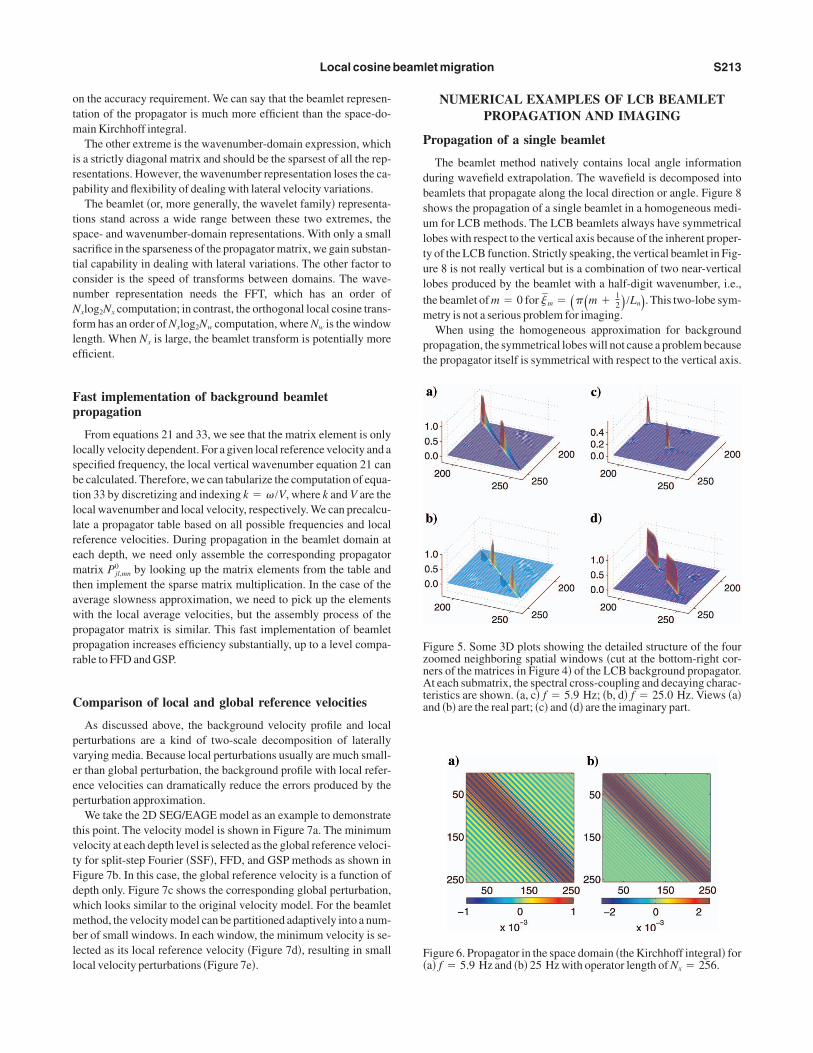
Pjl,mn0 is usually a highly sparse matrix. Figure 4 shows the sparsenessf the LCB propagator in a homogeneous background. Figure 4a andis for f � 5.9 Hz, and Figure 4b and d is for f � 25.0 Hz; Figurea and b shows the real part of the propagators, and Figure 4c and dhows the imaginary part.

Figure 5 shows the detailed structure of the two zoomed beamletropagators in a form of a 3D plot for four neighboring spatial win-ows situated at the lower-right corners of the propagator matrices inigure 4. At each window, the corresponding submatrix shows thepectral coupling between the input and output. The low- and high-avenumber components correspond to the small- and large-angleaves, respectively.For comparison, we plot the corresponding propagator in the

pace domain �the Kirchhoff integral� in Figure 6. The space-domainropagator is a full matrix, and truncating the operator at a finiteength �operator aperture� will result in errors and artifacts. Howev-r, the beamlet propagator matrix is similar to eigenfunction expan-ion, where insignificant coefficients decay much faster than withhe space-domain operator. In fact, discarding the insignificant coef-cients does not lose operator aperture at all. In practice, we can set a

hreshold for operator compression, such as 10�3–10�7, depending

otm

irp

tsstcnNfle

Fp

lsbtllremtawppr

C

pveep

tvtFdwmbll

P

dbsultultm

pt

FznAta

F�

Local cosine beamlet migration S213

n the accuracy requirement. We can say that the beamlet represen-ation of the propagator is much more efficient than the space-do-

ain Kirchhoff integral.The other extreme is the wavenumber-domain expression, which

s a strictly diagonal matrix and should be the sparsest of all the rep-esentations. However, the wavenumber representation loses the ca-ability and flexibility of dealing with lateral velocity variations.

The beamlet �or, more generally, the wavelet family� representa-ions stand across a wide range between these two extremes, thepace- and wavenumber-domain representations. With only a smallacrifice in the sparseness of the propagator matrix, we gain substan-ial capability in dealing with lateral variations. The other factor toonsider is the speed of transforms between domains. The wave-umber representation needs the FFT, which has an order of

xlog2Nx computation; in contrast, the orthogonal local cosine trans-orm has an order of Nxlog2Nw computation, where Nw is the windowength. When Nx is large, the beamlet transform is potentially morefficient.

ast implementation of background beamletropagation

From equations 21 and 33, we see that the matrix element is onlyocally velocity dependent. For a given local reference velocity and apecified frequency, the local vertical wavenumber equation 21 cane calculated. Therefore, we can tabularize the computation of equa-ion 33 by discretizing and indexing k � /V, where k and V are theocal wavenumber and local velocity, respectively. We can precalcu-ate a propagator table based on all possible frequencies and localeference velocities. During propagation in the beamlet domain atach depth, we need only assemble the corresponding propagatoratrix Pjl,mn

0 by looking up the matrix elements from the table andhen implement the sparse matrix multiplication. In the case of theverage slowness approximation, we need to pick up the elementsith the local average velocities, but the assembly process of theropagator matrix is similar. This fast implementation of beamletropagation increases efficiency substantially, up to a level compa-able to FFD and GSP.

omparison of local and global reference velocities

As discussed above, the background velocity profile and localerturbations are a kind of two-scale decomposition of laterallyarying media. Because local perturbations usually are much small-r than global perturbation, the background profile with local refer-nce velocities can dramatically reduce the errors produced by theerturbation approximation.

We take the 2D SEG/EAGE model as an example to demonstratehis point. The velocity model is shown in Figure 7a. The minimumelocity at each depth level is selected as the global reference veloci-y for split-step Fourier �SSF�, FFD, and GSP methods as shown inigure 7b. In this case, the global reference velocity is a function ofepth only. Figure 7c shows the corresponding global perturbation,hich looks similar to the original velocity model. For the beamletethod, the velocity model can be partitioned adaptively into a num-

er of small windows. In each window, the minimum velocity is se-ected as its local reference velocity �Figure 7d�, resulting in smallocal velocity perturbations �Figure 7e�.

NUMERICAL EXAMPLES OF LCB BEAMLETPROPAGATION AND IMAGING

ropagation of a single beamlet

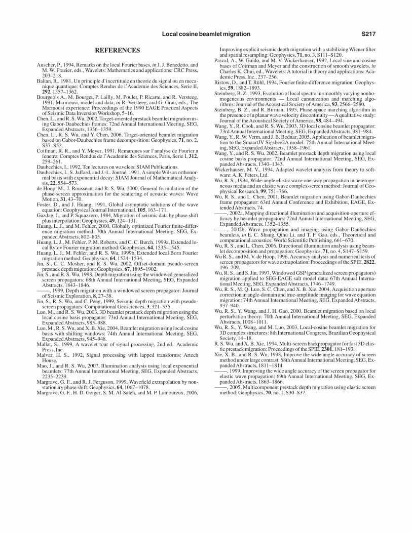
The beamlet method natively contains local angle informationuring wavefield extrapolation. The wavefield is decomposed intoeamlets that propagate along the local direction or angle. Figure 8hows the propagation of a single beamlet in a homogeneous medi-m for LCB methods. The LCB beamlets always have symmetricalobes with respect to the vertical axis because of the inherent proper-y of the LCB function. Strictly speaking, the vertical beamlet in Fig-re 8 is not really vertical but is a combination of two near-verticalobes produced by the beamlet with a half-digit wavenumber, i.e.,he beamlet of m � 0 for � m � ���m �

12�/Ln�. This two-lobe sym-

etry is not a serious problem for imaging.When using the homogeneous approximation for background

ropagation, the symmetrical lobes will not cause a problem becausehe propagator itself is symmetrical with respect to the vertical axis.

igure 5. Some 3D plots showing the detailed structure of the fouroomed neighboring spatial windows �cut at the bottom-right cor-ers of the matrices in Figure 4� of the LCB background propagator.t each submatrix, the spectral cross-coupling and decaying charac-

eristics are shown. �a, c� f � 5.9 Hz; �b, d� f � 25.0 Hz. Views �a�nd �b� are the real part; �c� and �d� are the imaginary part.

igure 6. Propagator in the space domain �the Kirchhoff integral� fora� f � 5.9 Hz and �b� 25 Hz with operator length of N � 256.

x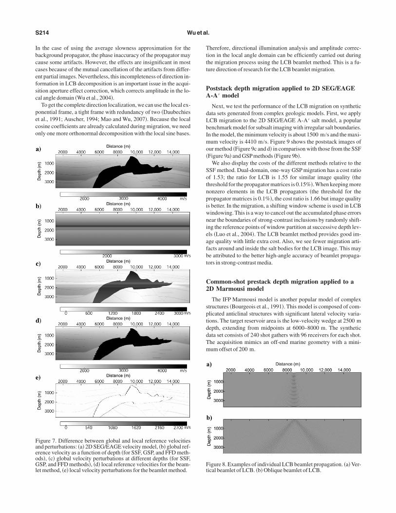

Ibccefsc

peco

Tttt

PA

dLbImo�

Sotnpiwnieafbt

C2

sptddTm

FaeoGl

Ft

S214 Wu et al.

n the case of using the average slowness approximation for theackground propagator, the phase inaccuracy of the propagator mayause some artifacts. However, the effects are insignificant in mostases because of the mutual cancellation of the artifacts from differ-nt partial images. Nevertheless, this incompleteness of direction in-ormation in LCB decomposition is an important issue in the acqui-ition aperture effect correction, which corrects amplitude in the lo-al angle domain �Wu et al., 2004�.

To get the complete direction localization, we can use the local ex-onential frame, a tight frame with redundancy of two �Daubechiest al., 1991; Auscher, 1994; Mao and Wu, 2007�. Because the localosine coefficients are already calculated during migration, we neednly one more orthonormal decomposition with the local sine bases.

igure 7. Difference between global and local reference velocitiesnd perturbations: �a� 2D SEG/EAGE velocity model, �b� global ref-rence velocity as a function of depth �for SSF, GSP, and FFD meth-ds�, �c� global velocity perturbations at different depths �for SSF,SP, and FFD methods�, �d� local reference velocities for the beam-

et method, �e� local velocity perturbations for the beamlet method.

herefore, directional illumination analysis and amplitude correc-ion in the local angle domain can be efficiently carried out duringhe migration process using the LCB beamlet method. This is a fu-ure direction of research for the LCB beamlet migration.

oststack depth migration applied to 2D SEG/EAGE-A� model

Next, we test the performance of the LCB migration on syntheticata sets generated from complex geologic models. First, we applyCB migration to the 2D SEG/EAGE A-A� salt model, a popularenchmark model for subsalt imaging with irregular salt boundaries.n the model, the minimum velocity is about 1500 m/s and the maxi-um velocity is 4410 m/s. Figure 9 shows the poststack images of

ur method �Figure 9c and d� in comparison with those from the SSFFigure 9a� and GSP methods �Figure 9b�.

We also display the costs of the different methods relative to theSF method. Dual-domain, one-way GSP migration has a cost ratiof 1.53; the ratio for LCB is 1.55 for similar image quality �thehreshold for the propagator matrices is 0.15%�. When keeping moreonzero elements in the LCB propagators �the threshold for theropagator matrices is 0.1%�, the cost ratio is 1.66 but image qualitys better. In the migration, a shifting window scheme is used in LCBindowing. This is a way to cancel out the accumulated phase errorsear the boundaries of strong-contrast inclusions by randomly shift-ng the reference points of window partition at successive depth lev-ls �Luo et al., 2004�. The LCB beamlet method provides good im-ge quality with little extra cost. Also, we see fewer migration arti-acts around and inside the salt bodies for the LCB image. This maye attributed to the better high-angle accuracy of beamlet propaga-ors in strong-contrast media.

ommon-shot prestack depth migration applied to aD Marmousi model

The IFP Marmousi model is another popular model of complextructures �Bourgeois et al., 1991�. This model is composed of com-licated anticlinal structures with significant lateral velocity varia-ions. The target reservoir area is the low-velocity wedge at 2500 mepth, extending from midpoints at 6000–8000 m. The syntheticata set consists of 240 shot gathers with 96 receivers for each shot.he acquisition mimics an off-end marine geometry with a mini-um offset of 200 m.

a)

b)

igure 8. Examples of individual LCB beamlet propagation. �a� Ver-ical beamlet of LCB. �b� Oblique beamlet of LCB.

tpumqr

C

uctnhBTgt

mtg

LdlL

Ft�C0t

Fe�m

Ft

Local cosine beamlet migration S215

Figure 10a is the Marmousi velocity model, and Figure 10b showshe shot-record prestack depth migration �PSDM� result by thehase-screen �SSF� method with minimum reference velocity. Fig-re 10c gives the shot-profile PSDM result by the LCB beamletethod. The LCB beamlet method achieves much better image

uality than the phase-screen method, particularly for the deep targeteservoir area and anticlines.

ommon-shot PSDM applied to 2D Sigsbee2A model

The benchmark data Sigsbee2A from the Smaart joint venture issed here to see the image quality of LCB beamlet migration for thisomplex salt structure and different scattering objects. The acquisi-ion has 500 shots with right-hand-side receivers; the maximumumber of receivers for one shot is 348. The original velocity modelas 3201 samples in horizontal extent and 1200 samples in depth.oth sample intervals are 7.6 m �25 feet�, as shown in Figure 11a.he image by the LCB method is shown in Figure 11b. We see theood image quality of LCB migration in this complex geologic set-ing.

DISCUSSION

We discuss here the advantages and disadvantages of the LCBethod compared to the beamlet migration using the GDF propaga-

or �Wu and Chen, 2001; Chen et al., 2006�. The LCB beamlet mi-ration is much more efficient than the GDF method because the

igure 9. Comparison of image quality and cost of poststack migra-ion on the 2D SEG/EAGE A-A� salt model by different methods.a� SSF method. Computing cost is set to 1.00. �b� GSP method.omputing cost is �1.53. �c� LCB method �propagator threshold.15%�. Computing cost is �1.55. �d� LCB method �propagatorhreshold 0.1%�. Computing cost is �1.66.

CB is an orthonormal basis. In contrast, the GDF has redundancy inecomposition. When the redundancy is two, as normally used in theiterature, the propagator matrix is four times larger than that of theCB in the 2D case. However, the redundancy in the GDF propaga-

igure 10. Comparisons of migration results for the Marmousi mod-l. �a� Velocity model. �b� Prestack image from the phase-screenSSF� migration method. �c� Prestack image from the LCB beamletigration method.

a)

b)

igure 11. �a� Velocity model. �b� Prestack image by LCB method ofhe 2D Sigsbee2Asalt model.

tcd

otweWpwtutBmTcdd

oltcbasppel

oqsLoitt

fRStacct

B

is�vfaa

F

b�cTtbU

�

T�i

E

tfoepc

F

tt

S216 Wu et al.

or may result in fewer migration artifacts. Also, the GDF methodan be approximated easily by asymptotic solutions in smooth me-ia.

An important special feature of the LCB beamlet migration meth-d, similar to other beamlet methods, is the availability of informa-ion in the local wavenumber domain. This information in the localavenumber domain can be used to correct the acquisition aperture

ffect and for other processing related to the local angle domain �seeu et al., 2004�. However, we know that LCB beamlets have incom-

lete direction information, i.e., they always have symmetrical lobesith respect to the vertical axis because of the inherent property of

he LCB function. To get the complete direction localization, we canse the local exponential frame, a tight frame with a redundancy ofwo �Daubechies et al., 1991; Auscher, 1994; Mao and Wu, 2007�.ecause the local cosine coefficients are already calculated duringigration, we only need one more orthonormal decomposition.herefore, illumination analysis, resolution analysis, and amplitudeorrection in the local-angle domain can be carried out efficientlyuring migration using the LCB beamlet method. This is one futureirection of research for LCB beamlet migration.

CONCLUSION

We have presented the theoretical foundation and technical detailsf a migration method using an LCB beamlet propagator. The beam-et propagator in heterogeneous media based on local perturbationheory has been derived, and a fast implementation method has beenonstructed. The use of local background velocity and local pertur-ations results in a two-scale decomposition of beamlet propagators:background propagator for large-scale structures and a local phase-creen correction for small-scale local perturbations. The beamletropagator can handle strong lateral velocity variations with im-roved accuracy. For the LCB, the propagator matrices are calculat-d efficiently using a table-driven method; propagation in the beam-et domain is implemented by sparse matrix operations.

The numerical examples demonstrate the accuracy and efficiencyf this approach. Compared with the FFD and GSP methods, imageuality and computational efficiency are similar. In some cases, weee fewer migration artifacts around and inside the salt bodies for theCB image. This may be attributed to the better high-angle accuracyf beamlet propagators in strong-contrast media. The availability ofnformation in the local angle domain of LCB migration is an impor-ant feature and can be utilized for acquisition aperture effect correc-ion and other processing related to local angle spectra.

ACKNOWLEDGMENTS

The authors acknowledge the support from the Wavelet Trans-orm on Propagation and Imaging for Seismic Exploration �WTOPI�esearch Consortium and the Department of Energy/Basic Energyciences project at the University of California, Santa Cruz. We

hank all of the industrial sponsors of our research consortium. Welso thank Jun Cao, Xiao-Bi Xie, Shengwen Jin, Chuck Mosher, Ri-hard W. Verm, Richard Cook, and M. Lee Bell for the helpful dis-ussions and suggestions. We are grateful to Smaart JV for providinghe Sigsbee2Asynthetic data set.

APPENDIX A

FAST ALGORITHM OF LCT

ell (window) function

The bell �window� function Bn�x� over the interval In � �xn, xn�1�s defined by the equations 2–5 in the text. From equation 3, we canhow that � k�1��x � xn�/�� has �2k � 1� vanishing derivatives at x

xn � � and x � xn � �, and � k�1��xn�1 � x�/��� has �2k � 1�anishing derivatives at x � xn�1 � �� and x � xn�1 � ��. There-ore, � k�1��x � xn�/�� or � k�1��xn�1 � x�/��� can be made into anrbitrarily smooth shape function. We set k � 2 in our numerical ex-mples.

olding

Instead of calculating inner products with the LCB elementsmn�x� having overlapping intervals, we can preprocess wavefieldsdata� so that the standard fast discrete cosine transform algorithman be used for efficient computation �e.g., Wickerhauser, 1994�.his can be realized by folding the overlapping parts of the bell func-

ions back into the intervals. Suppose we wish to fold a signal f�x�ack into the interval In � �xn, xn�1� across xn and xn�1 �Figure 1b�.sing the bell function Bn�x� defined by equation 2, we have

fnew�x�

� f��x� � Bn�x�f�x� � Bn�2xn � x�f�2xn � x� , if xn � x � xn � �

f��x� � Bn�x�f�x� � Bn�2xn�1 � x�f�2xn�1 � x� , if xn�1 � �� � x � xn�1

f�x� , if xn � � � x � xn�1 � �� .

�A-1�he resultant folded data fnew�x� is now defined in the interval In

�xn, xn�1�. To reconstruct f�x� from fnew�x�, we can use the follow-ng unfolding formulas:

f�x�

� � Bn�x�fnew�x� � Bn�2xn � x�fnew�2xn � x� , if xn � x � xn � �

Bn�x�fnew�x� � Bn�2xn�1 � x�fnew�2xn�1 � x� , if xn�1 � �� � x � xn�1

fnew�x� , if xn � � � x � xn�1 � �� .

�A-2�

dge extension

When the bell shifts to the leftmost or the rightmost endpoint ofhe signal, we cannot directly obtain f��x� or f��x� from the aboveormulas because of the lack of data in the leftmost and rightmostverlapping zones. Four extension methods are available: �1� zeroxtension, �2� symmetry extension, �3� smooth extension, and �4�eriodization extension. Based on the features of seismic signals, wehose the zero-extension method.

ast DCT

After the procedures of folding and edge extension, we can applyhe fast DCT to the folded data fnew�x� to obtain the local cosineransform coefficients.

A

B

B

C

C

C

DD

d

F

G

H

H

H

J

J

—

J

L

L

M

M

M

M

M

P

R

S

S

W

W

W

W

W

W

—

—

W

W

W

W

W

W

R

X

—

—

Local cosine beamlet migration S217

REFERENCES

uscher, P., 1994, Remarks on the local Fourier bases, in J. J. Benedetto, andM. W. Frazier, eds., Wavelets: Mathematics and applications: CRC Press,203–218.

alian, R., 1981, Un principle d’incertitude en theorie du signal ou en meca-nique quantique: Comptes Rendus de l’Academie des Sciences, Serie II,292, 1357–1362.

ourgeois A., M. Bourget, P. Lailly, M. Poulet, P. Ricarte, and R. Versteeg,1991, Marmousi, model and data, in R. Versteeg, and G. Grau, eds., TheMarmousi experience: Proceedings of the 1990 EAGE Practical Aspectsof Seismic Data Inversion Workshop, 5–16.

hen, L., and R. S. Wu, 2002, Target-oriented prestack beamlet migration us-ing Gabor-Daubechies frames: 72nd Annual International Meeting, SEG,ExpandedAbstracts, 1356–1359.

hen, L., R. S. Wu, and Y. Chen, 2006, Target-oriented beamlet migrationbased on Gabor-Daubechies frame decomposition: Geophysics, 71, no. 2,S37–S52.

oifman, R. R., and Y. Meyer, 1991, Remarques sur l’analyse de Fourier afenetre: Comptes Rendus de l’Academie des Sciences, Paris, Serie I, 312,259–261.

aubechies, I., 1992, Ten lectures on wavelets: SIAM Publications.aubechies, I., S. Jaffard, and J.-L. Journé, 1991, A simple Wilson orthonor-mal basis with exponential decay: SIAM Journal of Mathematical Analy-sis, 22, 554–573.

e Hoop, M., J. Rousseau, and R. S. Wu, 2000, General formulation of thephase-screen approximation for the scattering of acoustic waves: WaveMotion, 31, 43–70.

oster, D., and J. Huang, 1991, Global asymptotic solutions of the waveequation: Geophysical Journal International, 105, 163–171.

azdag, J., and P. Squazzero, 1984, Migration of seismic data by phase shiftplus interpolation: Geophysics, 49, 124–131.

uang, L. J., and M. Fehler, 2000, Globally optimized Fourier finite-differ-ence migration method: 70th Annual International Meeting, SEG, Ex-pandedAbstracts, 802–805.

uang, L. J., M. Fehler, P. M. Roberts, and C. C. Burch, 1999a, Extended lo-cal Rytov Fourier migration method: Geophysics, 64, 1535–1545.

uang, L. J., M. Fehler, and R. S. Wu, 1999b, Extended local Born Fouriermigration method: Geophysics, 64, 1524–1534.

in, S., C. C. Mosher, and R. S. Wu, 2002, Offset-domain pseudo-screenprestack depth migration: Geophysics, 67, 1895–1902.

in, S., and R. S. Wu, 1998, Depth migration using the windowed generalizedscreen propagators: 68th Annual International Meeting, SEG, ExpandedAbstracts, 1843–1846.—–, 1999, Depth migration with a windowed screen propagator: Journalof Seismic Exploration, 8, 27–38.

in, S., R. S. Wu, and C. Peng, 1999, Seismic depth migration with pseudo-screen propagators: Computational Geosciences, 3, 321–335.

uo, M., and R. S. Wu, 2003, 3D beamlet prestack depth migration using thelocal cosine basis propagator: 73rd Annual International Meeting, SEG,ExpandedAbstracts, 985–988.

uo, M., R. S. Wu, and X. B. Xie, 2004, Beamlet migration using local cosinebasis with shifting windows: 74th Annual International Meeting, SEG,ExpandedAbstracts, 945–948.allat, S., 1999, A wavelet tour of signal processing, 2nd ed.: AcademicPress, Inc.alvar, H. S., 1992, Signal processing with lapped transforms: ArtechHouse.ao, J., and R. S. Wu, 2007, Illumination analysis using local exponentialbeamlets: 77th Annual International Meeting, SEG, Expanded Abstracts,2235–2239.argrave, G. F., and R. J. Ferguson, 1999, Wavefield extrapolation by non-stationary phase shift: Geophysics, 64, 1067–1078.

argrave, G. F., H. D. Geiger, S. M. Al-Saleh, and M. P. Lamoureux, 2006,

Improving explicit seismic depth migration with a stabilizing Wiener filterand spatial resampling: Geophysics, 71, no. 3, S111–S120.

ascal, A., W. Guido, and M. V. Wickerhauser, 1992, Local sine and cosinebases of Coifman and Meyer and the construction of smooth wavelets, inCharles K. Chui, ed., Wavelets: A tutorial in theory and applications: Aca-demic Press, Inc., 237–256.

istow, D., and T. Rühl, 1994, Fourier finite-difference migration: Geophys-ics, 59, 1882–1893.

teinberg, B. Z., 1993, Evolution of local spectra in smoothly varying nonho-mogeneous environments — Local canonization and marching algo-rithms: Journal of theAcoustical Society ofAmerica, 93, 2566–2580.

teinberg, B. Z., and R. Birman, 1995, Phase-space marching algorithm inthe presence of a planar wave velocity discontinuity —Aqualitative study:Journal of theAcoustical Society ofAmerica, 98, 484–494.ang, Y., R. Cook, and R. S. Wu, 2003, 3D local cosine beamlet propagator:73rdAnnual International Meeting, SEG, ExpandedAbstracts, 981–984.ang, Y., R. W. Verm, and J. B. Bednar, 2005, Application of beamlet migra-tion to the SmaartJV Sigsbee2A model: 75th Annual International Meet-ing, SEG, ExpandedAbstracts, 1958–1961.ang, Y., and R. S. Wu, 2002, Beamlet prestack depth migration using localcosine basis propagator: 72nd Annual International Meeting, SEG, Ex-pandedAbstracts, 1340–1343.ickerhauser, M. V., 1994, Adapted wavelet analysis from theory to soft-ware:A. K. Peters, Ltd.u, R. S., 1994, Wide-angle elastic wave one-way propagation in heteroge-neous media and an elastic wave complex-screen method: Journal of Geo-physical Research, 99, 751–766.u, R. S., and L. Chen, 2001, Beamlet migration using Gabor-Daubechiesframe propagator: 63rd Annual Conference and Exhibition, EAGE, Ex-tendedAbstracts, 74.—–, 2002a, Mapping directional illumination and acquisition-aperture ef-ficacy by beamlet propagators: 72nd Annual International Meeting, SEG,ExpandedAbstracts, 1352–1355.—–, 2002b, Wave propagation and imaging using Gabor-Daubechiesbeamlets, in E. C. Shang, Qihu Li, and T. F. Gao, eds., Theoretical andcomputational acoustics: World Scientific Publishing, 661–670.u, R. S., and L. Chen, 2006, Directional illumination analysis using beam-let decomposition and propagation: Geophysics, 71, no. 4, S147–S159.u R. S., and M. V. de Hoop, 1996, Accuracy analysis and numerical tests ofscreen propagators for wave extrapolation: Proceedings of the SPIE, 2822,196–209.u, R. S., and S. Jin, 1997, Windowed GSP �generalized screen propagators�migration applied to SEG-EAGE salt model data: 67th Annual Interna-tional Meeting, SEG, ExpandedAbstracts, 1746–1749.u, R. S., M. Q. Luo, S. C. Chen, and X. B. Xie, 2004, Acquisition aperturecorrection in angle-domain and true-amplitude imaging for wave equationmigration: 74th Annual International Meeting, SEG, Expanded Abstracts,937–940.u, R. S., Y. Wang, and J. H. Gao, 2000, Beamlet migration based on localperturbation theory: 70th Annual International Meeting, SEG, ExpandedAbstracts, 1008–1011.u, R. S., Y. Wang, and M. Luo, 2003, Local-cosine beamlet migration for3D complex structures: 8th International Congress, Brazilian GeophysicalSociety, 14–18.

. S. Wu, and X. B. Xie, 1994, Multi-screen backpropagator for fast 3D elas-tic prestack migration: Proceedings of the SPIE, 2301, 181–193.

ie, X. B., and R. S. Wu, 1998, Improve the wide angle accuracy of screenmethod under large contrast: 68thAnnual International Meeting, SEG, Ex-pandedAbstracts, 1811–1814.—–, 1999, Improving the wide angle accuracy of the screen propagator forelastic wave propagation: 69th Annual International Meeting, SEG, Ex-pandedAbstracts, 1863–1866.—–, 2005, Multicomponent prestack depth migration using elastic screen

method: Geophysics, 70, no. 1, S30–S37.