1

Before beginning, I would like to acknowledge the amazing contributions of Ken Nolte. I suspect that the origins of most of our discussion during this workshop can be traced to Dr. Nolte. He was a true “Legend of Hydraulic Fracturing.”

2

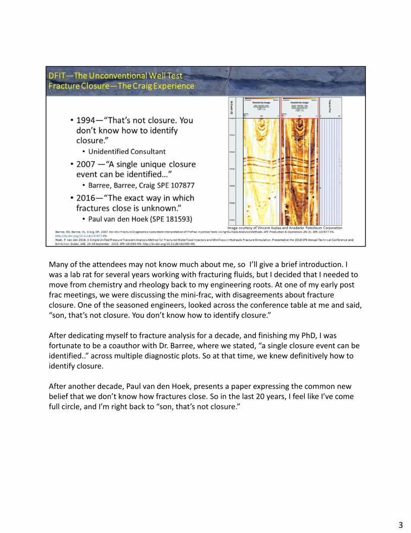
Many of the attendees may not know much about me, so  I’ll give a brief introduction. I was a lab rat for several years working with fracturing fluids, but I decided that I needed to move from chemistry and rheology back to my engineering roots. At one of my early post frac meetings, we were discussing the mini‐frac, with disagreements about fracture closure. One of the seasoned engineers, looked across the conference table at me and said, “son, that’s not closure. You don’t know how to identify closure.”

After dedicating myself to fracture analysis for a decade, and finishing my PhD, I was fortunate to be a coauthor with Dr. Barree, where we stated, “a single closure event can be identified..” across multiple diagnostic plots. So at that time, we knew definitively how to identify closure.

After another decade, Paul van den Hoek, presents a paper expressing the common new belief that we don’t know how fractures close. So in the last 20 years, I feel like I’ve come full circle, and I’m right back to “son, that’s not closure.”

3

I began DFIT testing specifically to determine pressure and permeability in about July 1998. The first DFIT well is shown in the picture. Western Colorado’s not a bad oilfield to work in, huh? 

4

The DFIT program we started in 1998 was hugely successful. By 2002 we have analyzed over 1,200 DFIT. At the time, reservoir pressure was estimated from closure and after‐closure flow regimes, and permeability was estimated from before‐closure analysis, and after closure when radial flow was observed.

But what about the majority of the data. Why wasn’t it used. Why couldn’t we use all the data…

5

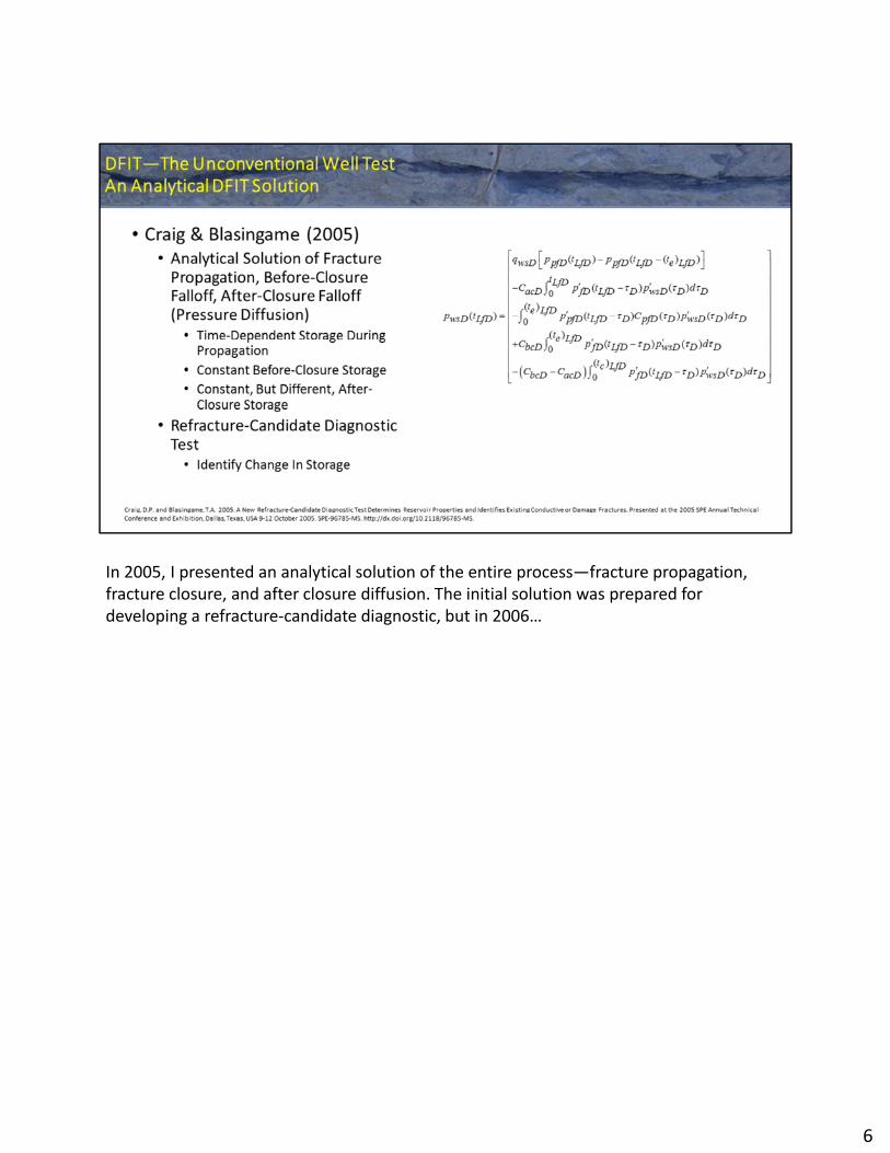
In 2005, I presented an analytical solution of the entire process—fracture propagation, fracture closure, and after closure diffusion. The initial solution was prepared for developing a refracture‐candidate diagnostic, but in 2006…

6

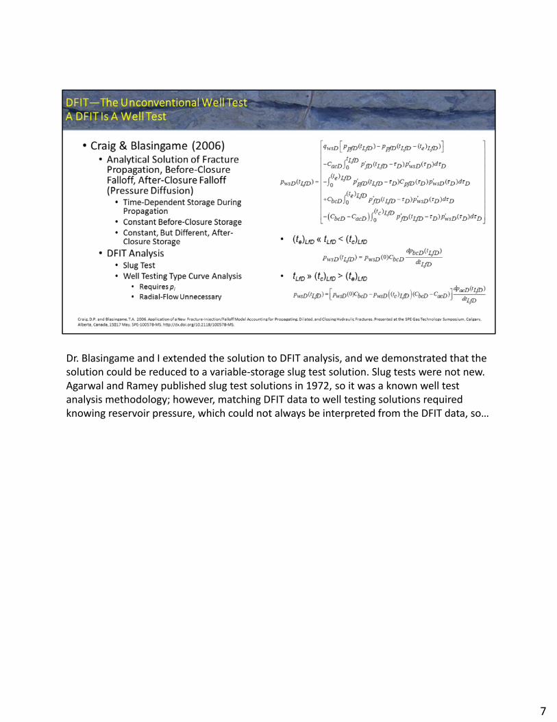
Dr. Blasingame and I extended the solution to DFIT analysis, and we demonstrated that the solution could be reduced to a variable‐storage slug test solution. Slug tests were not new. Agarwal and Ramey published slug test solutions in 1972, so it was a known well test analysis methodology; however, matching DFIT data to well testing solutions required knowing reservoir pressure, which could not always be interpreted from the DFIT data, so…

7

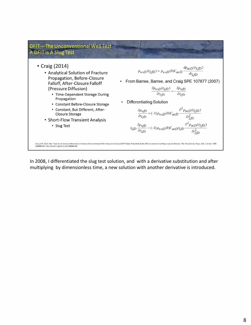
In 2008, I differentiated the slug test solution, and  with a derivative substitution and after multiplying  by dimensionless time, a new solution with another derivative is introduced.

8

While it may not look clear, the new solution is extremely powerful. It means the same semilog derivative used in the Barree holistic analysis method can be matched to a well‐testing type curve. From the match point reservoir pressure can be determined. With this new match, the well testing type curve analysis methodology was complete, and all DFIT could be analyzed by well testing methods. So let’s look at an example…

9

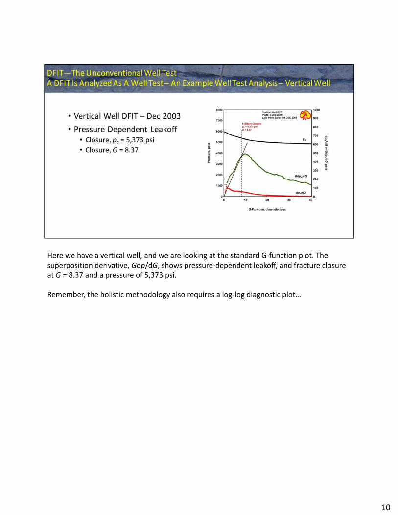
Here we have a vertical well, and we are looking at the standard G‐function plot. The superposition derivative, Gdp/dG, shows pressure‐dependent leakoff, and fracture closure at G = 8.37 and a pressure of 5,373 psi.

Remember, the holistic methodology also requires a log‐log diagnostic plot…

10

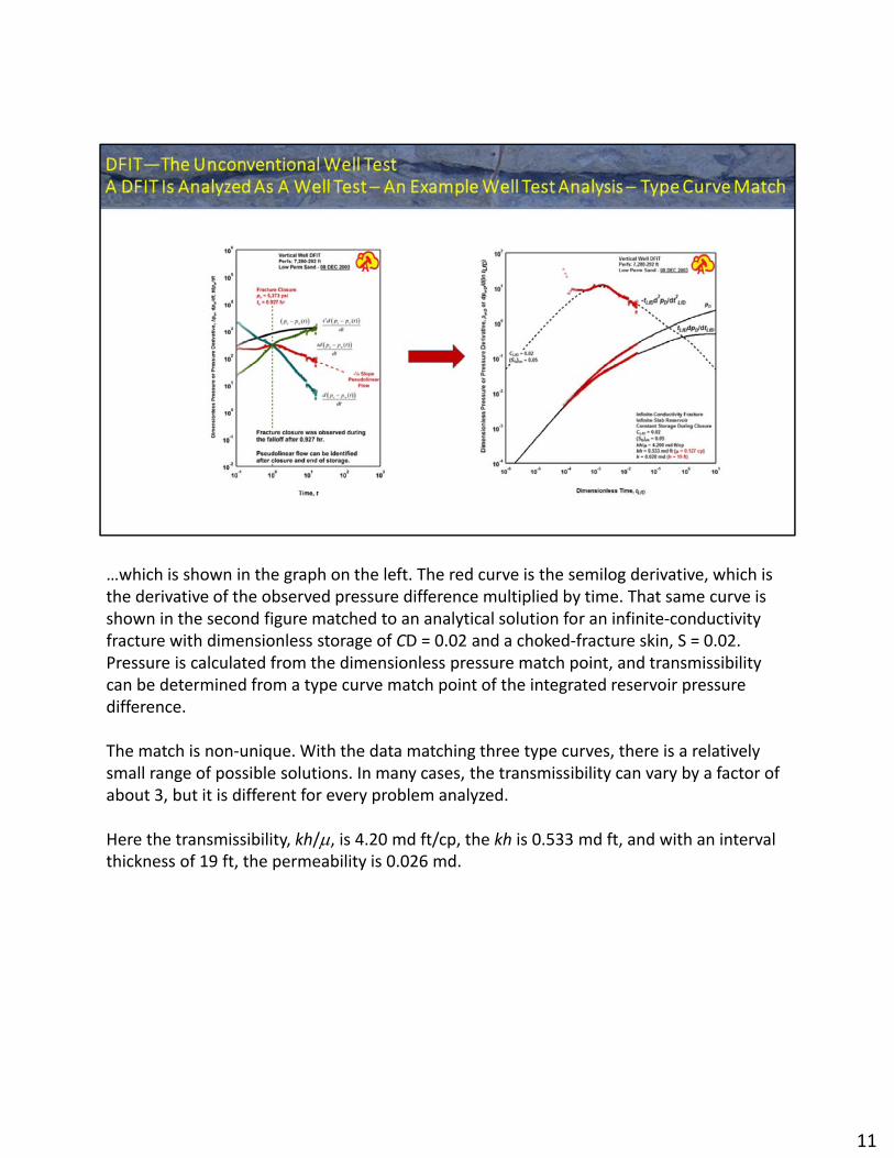
…which is shown in the graph on the left. The red curve is the semilog derivative, which is the derivative of the observed pressure difference multiplied by time. That same curve is shown in the second figure matched to an analytical solution for an infinite‐conductivity fracture with dimensionless storage of CD = 0.02 and a choked‐fracture skin, S = 0.02. Pressure is calculated from the dimensionless pressure match point, and transmissibility can be determined from a type curve match point of the integrated reservoir pressure difference.

The match is non‐unique. With the data matching three type curves, there is a relatively small range of possible solutions. In many cases, the transmissibility can vary by a factor of about 3, but it is different for every problem analyzed.

Here the transmissibility, kh/, is 4.20 md ft/cp, the kh is 0.533 md ft, and with an interval thickness of 19 ft, the permeability is 0.026 md.

11

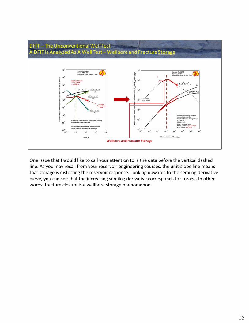
One issue that I would like to call your attention to is the data before the vertical dashed line. As you may recall from your reservoir engineering courses, the unit‐slope line means that storage is distorting the reservoir response. Looking upwards to the semilog derivative curve, you can see that the increasing semilog derivative corresponds to storage. In other words, fracture closure is a wellbore storage phenomenon.

12

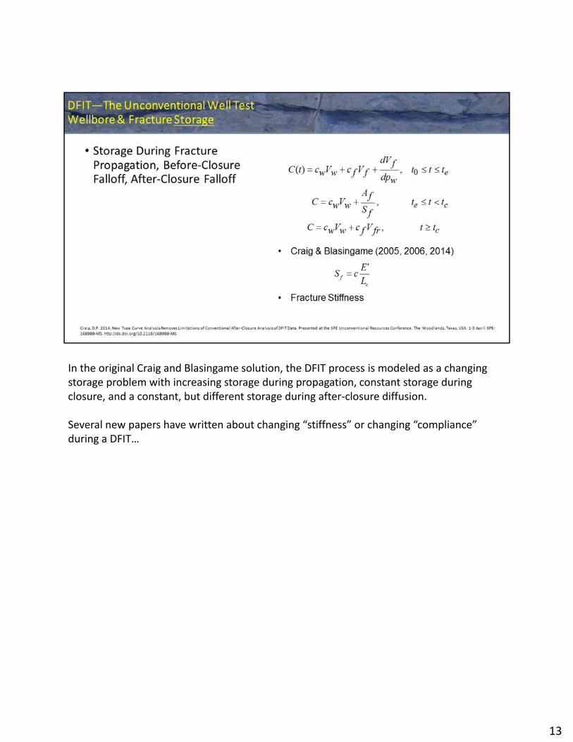
In the original Craig and Blasingame solution, the DFIT process is modeled as a changing storage problem with increasing storage during propagation, constant storage during closure, and a constant, but different storage during after‐closure diffusion.

Several new papers have written about changing “stiffness” or changing “compliance” during a DFIT…

13

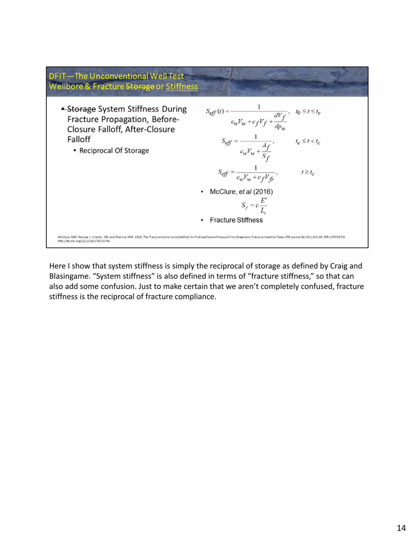
Here I show that system stiffness is simply the reciprocal of storage as defined by Craig and Blasingame. “System stiffness” is also defined in terms of “fracture stiffness,” so that can also add some confusion. Just to make certain that we aren’t completely confused, fracture stiffness is the reciprocal of fracture compliance.

14

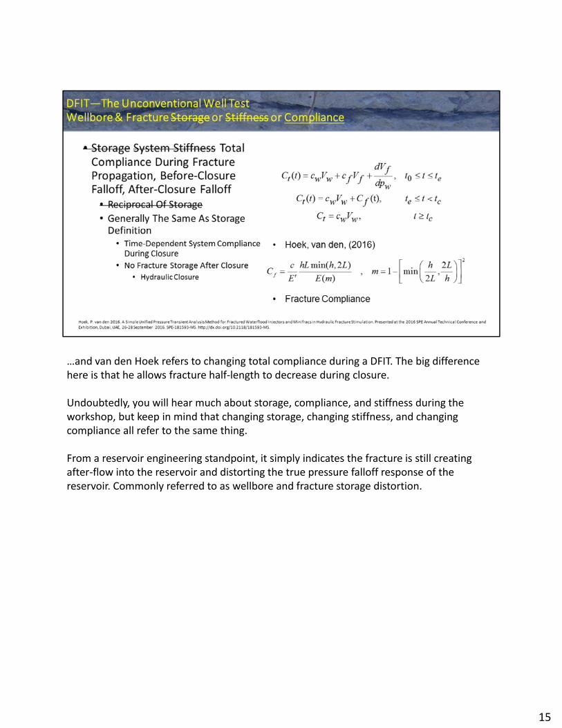
…and van den Hoek refers to changing total compliance during a DFIT. The big difference here is that he allows fracture half‐length to decrease during closure.

Undoubtedly, you will hear much about storage, compliance, and stiffness during the workshop, but keep in mind that changing storage, changing stiffness, and changing compliance all refer to the same thing. 

From a reservoir engineering standpoint, it simply indicates the fracture is still creating after‐flow into the reservoir and distorting the true pressure falloff response of the reservoir. Commonly referred to as wellbore and fracture storage distortion.

15

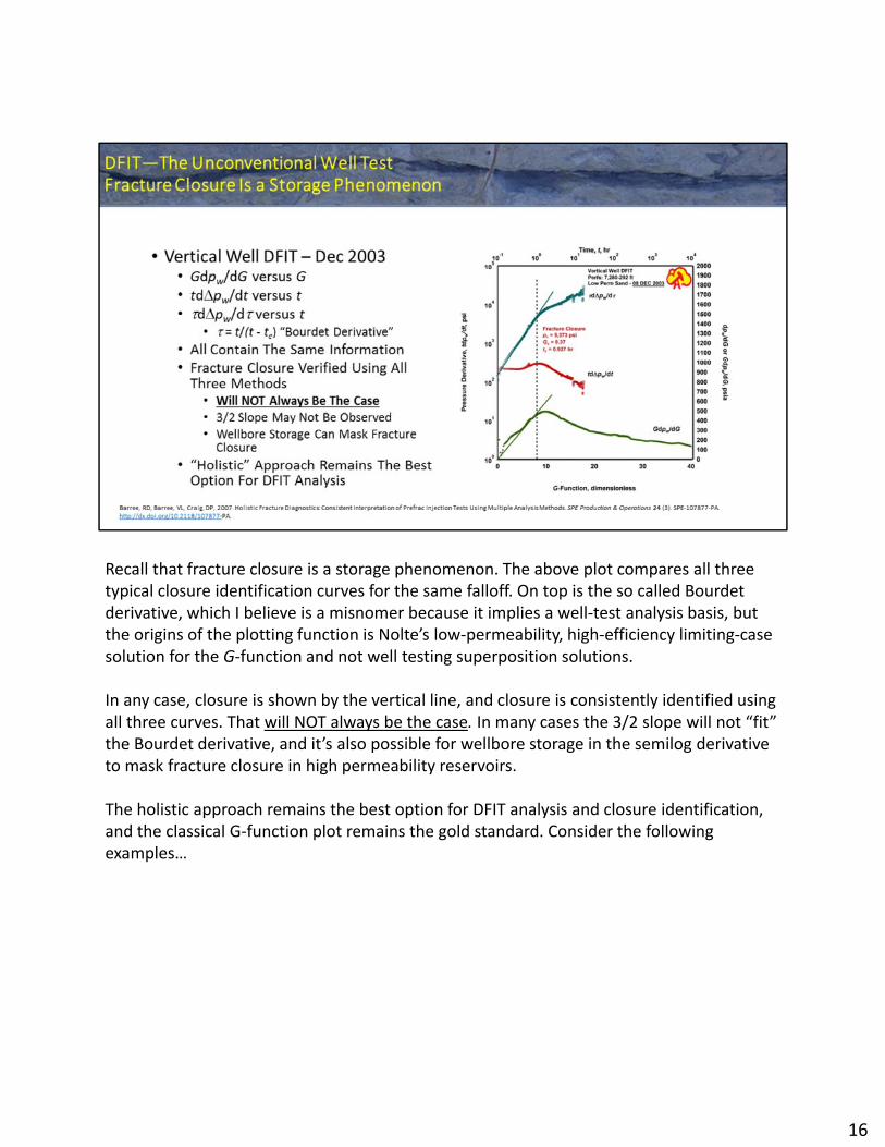
Recall that fracture closure is a storage phenomenon. The above plot compares all three typical closure identification curves for the same falloff. On top is the so called Bourdetderivative, which I believe is a misnomer because it implies a well‐test analysis basis, but the origins of the plotting function is Nolte’s low‐permeability, high‐efficiency limiting‐case solution for the G‐function and not well testing superposition solutions. 

In any case, closure is shown by the vertical line, and closure is consistently identified using all three curves. That will NOT always be the case. In many cases the 3/2 slope will not “fit” the Bourdet derivative, and it’s also possible for wellbore storage in the semilog derivative to mask fracture closure in high permeability reservoirs.

The holistic approach remains the best option for DFIT analysis and closure identification, and the classical G‐function plot remains the gold standard. Consider the following examples…

16

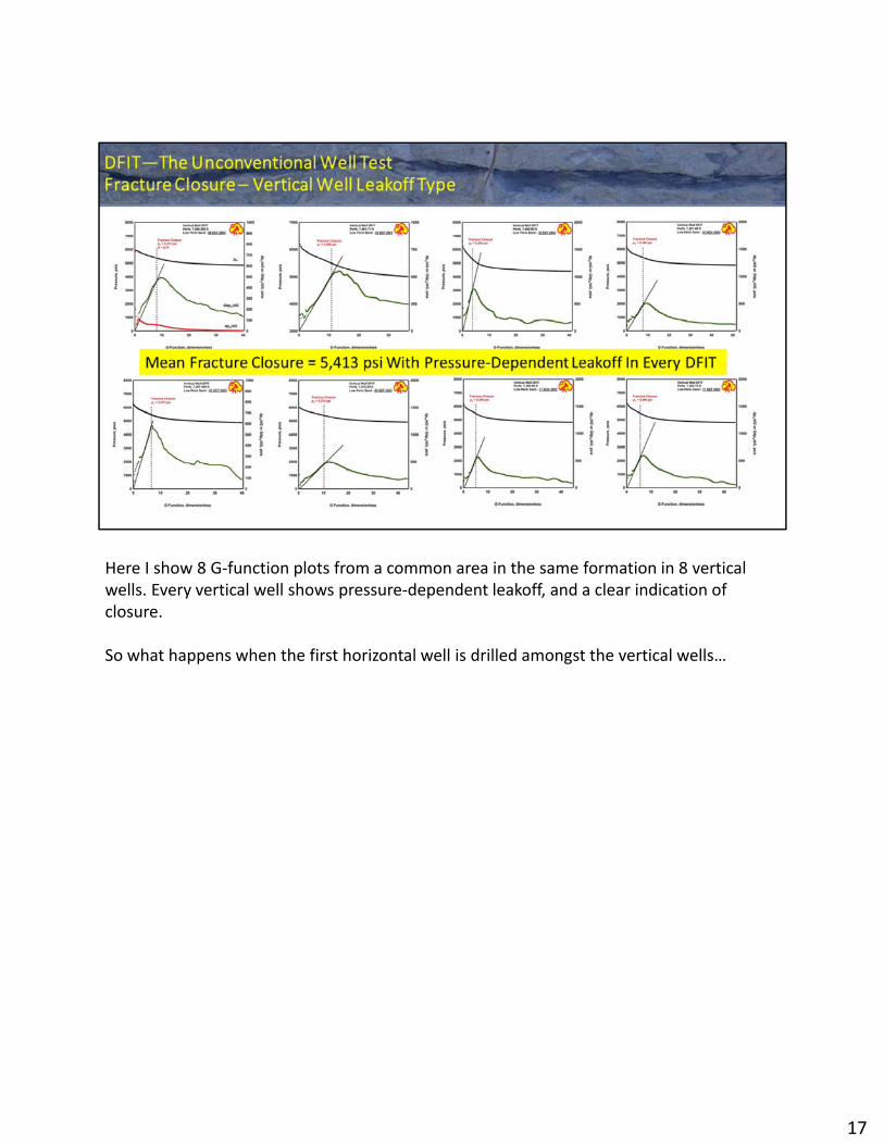
Here I show 8 G‐function plots from a common area in the same formation in 8 vertical wells. Every vertical well shows pressure‐dependent leakoff, and a clear indication of closure.

So what happens when the first horizontal well is drilled amongst the vertical wells…

17

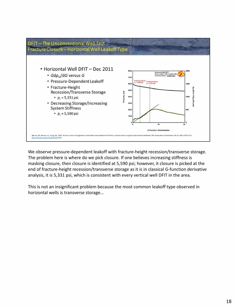
We observe pressure‐dependent leakoff with fracture‐height recession/transverse storage. The problem here is where do we pick closure. If one believes increasing stiffness is masking closure, then closure is identified at 5,590 psi; however, it closure is picked at the end of fracture‐height recession/transverse storage as it is in classical G‐function derivative analysis, it is 5,331 psi, which is consistent with every vertical well DFIT in the area.

This is not an insignificant problem because the most common leakoff type observed in horizontal wells is transverse storage…

18

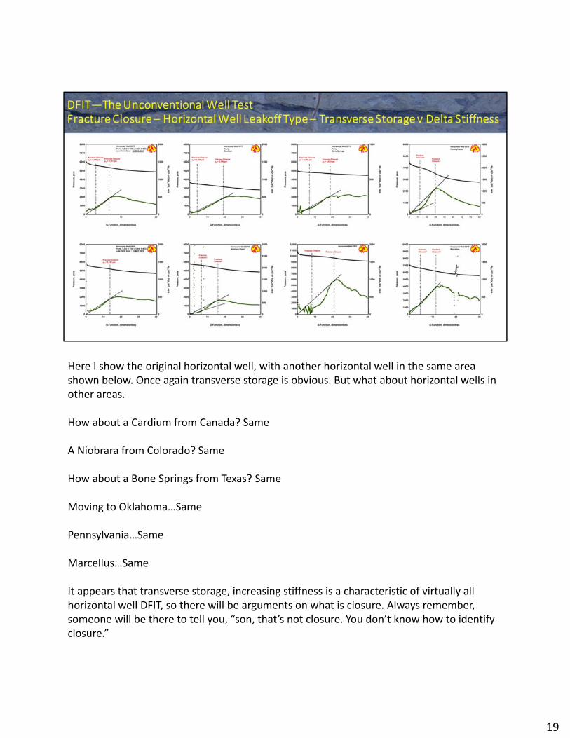
Here I show the original horizontal well, with another horizontal well in the same area shown below. Once again transverse storage is obvious. But what about horizontal wells in other areas.

How about a Cardium from Canada? Same

A Niobrara from Colorado? Same

How about a Bone Springs from Texas? Same

Moving to Oklahoma…Same

Pennsylvania…Same

Marcellus…Same

It appears that transverse storage, increasing stiffness is a characteristic of virtually all horizontal well DFIT, so there will be arguments on what is closure. Always remember, someone will be there to tell you, “son, that’s not closure. You don’t know how to identify closure.”

19

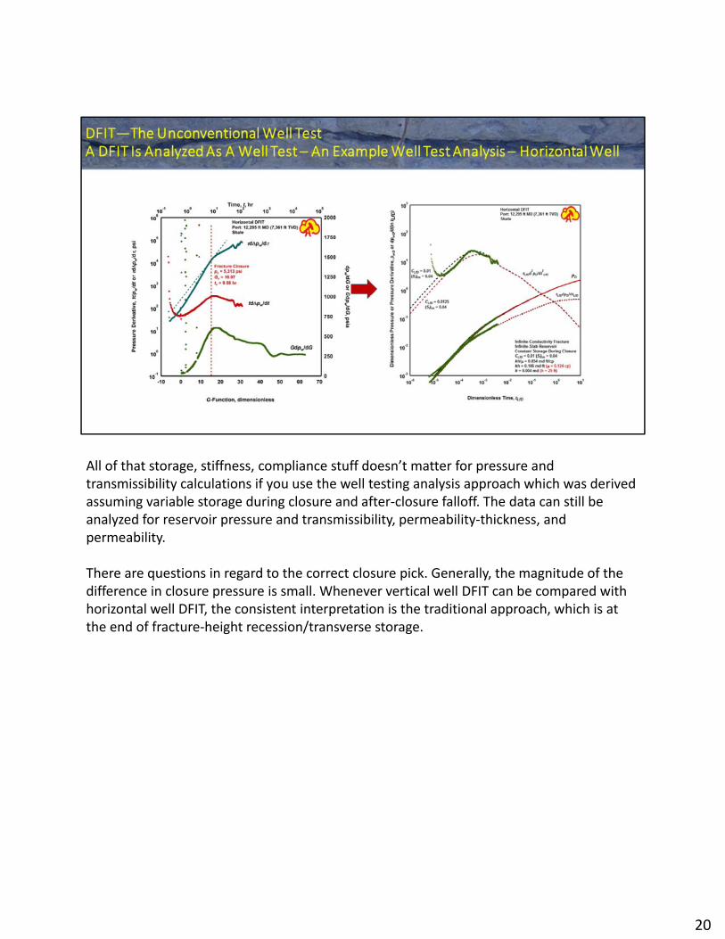
All of that storage, stiffness, compliance stuff doesn’t matter for pressure and transmissibility calculations if you use the well testing analysis approach which was derived assuming variable storage during closure and after‐closure falloff. The data can still be analyzed for reservoir pressure and transmissibility, permeability‐thickness, and permeability.

There are questions in regard to the correct closure pick. Generally, the magnitude of the difference in closure pressure is small. Whenever vertical well DFIT can be compared with horizontal well DFIT, the consistent interpretation is the traditional approach, which is at the end of fracture‐height recession/transverse storage.

20

21

22

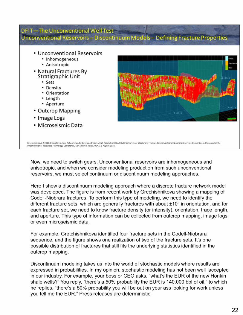
Now, we need to switch gears. Unconventional reservoirs are inhomogeneous and anisotropic, and when we consider modeling production from such unconventional reservoirs, we must select continuum or discontinuum modeling approaches.

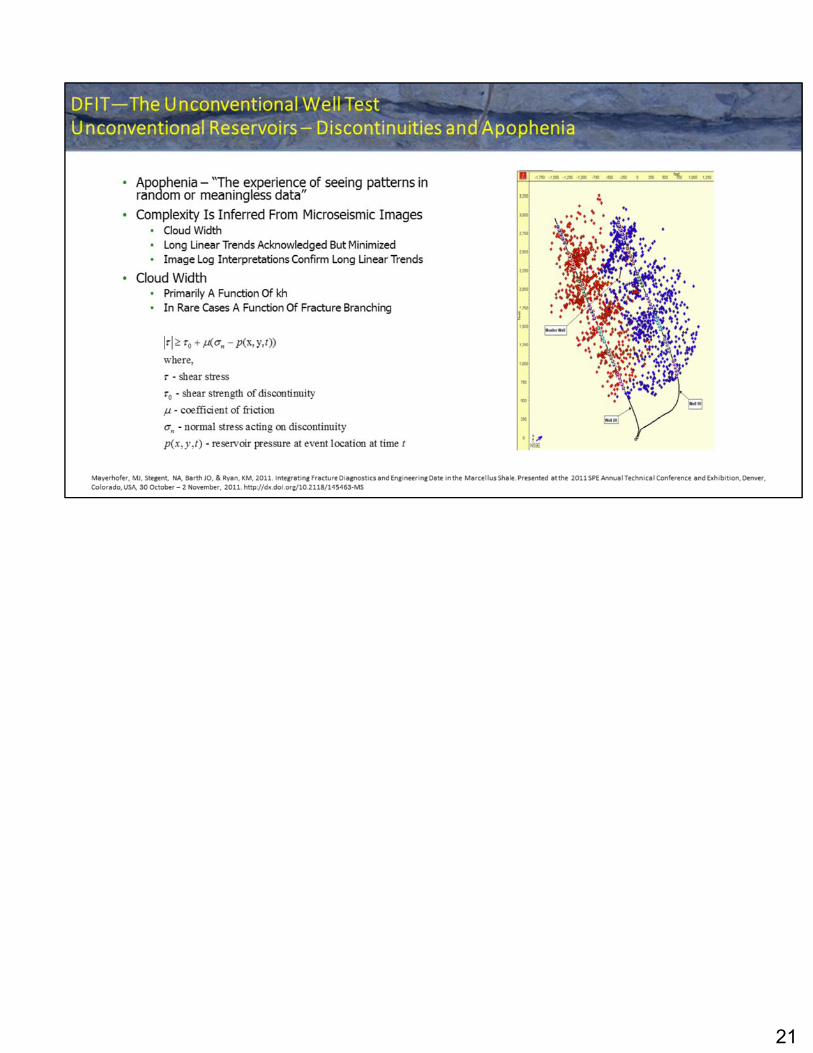
Here I show a discontinuum modeling approach where a discrete fracture network model was developed. The figure is from recent work by Grechishnikova showing a mapping of Codell-Niobrara fractures. To perform this type of modeling, we need to identify the different fracture sets, which are generally fractures with about ±10° in orientation, and for each fracture set, we need to know fracture density (or intensity), orientation, trace length, and aperture. This type of information can be collected from outcrop mapping, image logs, or even microseismic data.

For example, Gretchishnikova identified four fracture sets in the Codell-Niobrara sequence, and the figure shows one realization of two of the fracture sets. It’s one possible distribution of fractures that still fits the underlying statistics identified in the outcrop mapping.

Discontinuum modeling takes us into the world of stochastic models where results are expressed in probabilities. In my opinion, stochastic modeling has not been well accepted in our industry. For example, your boss or CEO asks, “what’s the EUR of the new Honkinshale wells?” You reply, “there’s a 50% probability the EUR is 140,000 bbl of oil,” to which he replies, “there’s a 50% probability you will be out on your ass looking for work unless you tell me the EUR.” Press releases are deterministic.

23

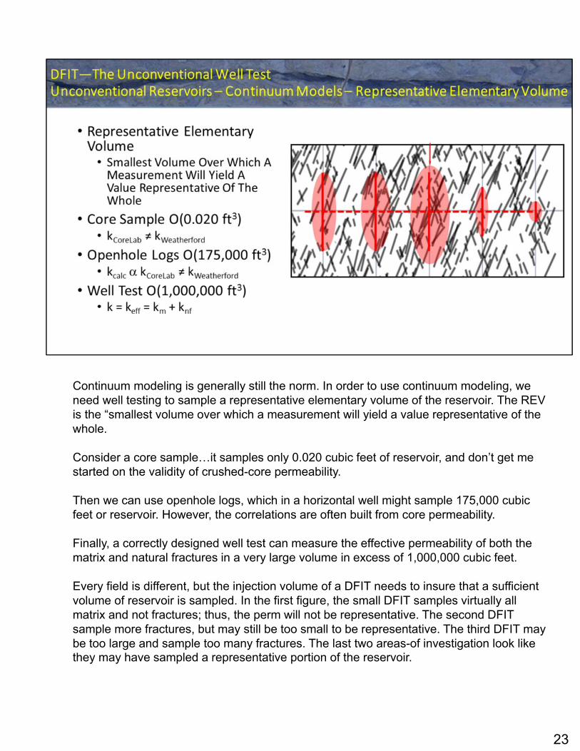
Continuum modeling is generally still the norm. In order to use continuum modeling, we need well testing to sample a representative elementary volume of the reservoir. The REV is the “smallest volume over which a measurement will yield a value representative of the whole.

Consider a core sample…it samples only 0.020 cubic feet of reservoir, and don’t get me started on the validity of crushed-core permeability.

Then we can use openhole logs, which in a horizontal well might sample 175,000 cubic feet or reservoir. However, the correlations are often built from core permeability.

Finally, a correctly designed well test can measure the effective permeability of both the matrix and natural fractures in a very large volume in excess of 1,000,000 cubic feet.

Every field is different, but the injection volume of a DFIT needs to insure that a sufficient volume of reservoir is sampled. In the first figure, the small DFIT samples virtually all matrix and not fractures; thus, the perm will not be representative. The second DFIT sample more fractures, but may still be too small to be representative. The third DFIT may be too large and sample too many fractures. The last two areas-of investigation look like they may have sampled a representative portion of the reservoir.

24

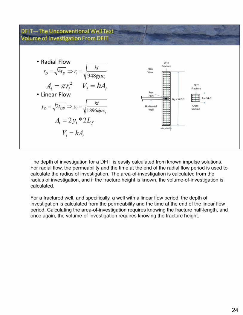
The depth of investigation for a DFIT is easily calculated from known impulse solutions. For radial flow, the permeability and the time at the end of the radial flow period is used to calculate the radius of investigation. The area-of-investigation is calculated from the radius of investigation, and if the fracture height is known, the volume-of-investigation is calculated.

For a fractured well, and specifically, a well with a linear flow period, the depth of investigation is calculated from the permeability and the time at the end of the linear flow period. Calculating the area-of-investigation requires knowing the fracture half-length, and once again, the volume-of-investigation requires knowing the fracture height.

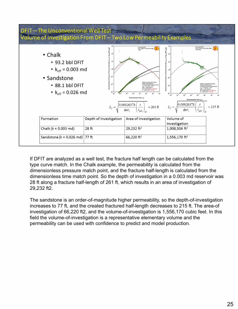
25

If DFIT are analyzed as a well test, the fracture half length can be calculated from the type curve match. In the Chalk example, the permeability is calculated from the dimensionless pressure match point, and the fracture half-length is calculated from the dimensionless time match point. So the depth of investigation in a 0.003 md reservoir was 28 ft along a fracture half-length of 261 ft, which results in an area of investigation of 29,232 ft2.

The sandstone is an order-of-magnitude higher permeability, so the depth-of-investigation increases to 77 ft, and the created fractured half-length decreases to 215 ft. The area-of investigation of 66,220 ft2, and the volume-of-investigation is 1,556,170 cubic feet. In this field the volume-of-investigation is a representative elementary volume and the permeability can be used with confidence to predict and model production.

26