An Alternative Theory of the Plant Size Distribution,

with Geography and Intra- and International Trade

Holmes and Stevens (forthcoming!)

Standard Theory of the Within—Industry Size Distribution

• New plants enter an industry and obtain a productivity draw.Plants that get good draws choose to be big. Lucas (1978)

• This idea has widespread use in international to explain tradefacts.

— Melitz

— Bernard, Eaton, Jensen Kortum (BEJK)

This Paper

• Observation: Even when we go to narrowly-defined industries,big plants often do not look like homothetic expansions of

smaller plants

• Plants of different size tend to do different functions. (Pioreand Sable (1984))

— Small plants: Specialty goods, craft production, (custom,

retail-like)

— Large plants: Standardized goods for inventory, mass pro-

duction

Example Industry that gets extra attention

• Wood Furniture

— Factories in North Carolina with 1000 plus employees make

stock furniture pieces

— Small craft shops scattered around the country, like Amish

furniture shops.

— NAICS industry classification puts them both in NAICS

337122

What We Do

• Theory of Geography and Trade applied to locations in theU.S.

— Standardized goods (off-the-shelf BEJK)

— Specialty goods

• Estimate the model

— Use Census micro data on the Commodity Flow Data

• Result 1: Estimate the share of establishment counts in thespecialty good segments

— In most industries, more then half the plants are specialtygood plants

— In most industries, the share is growing.

• Result 2: Concerns the plant size/industry concentration re-lationship

— Pure BEJK special case bombs quantitatively (can get thisqualitatively)

— Model with specialty goods segment added fits this

• Result 3: What happens when imports from China begin flow-ing into an industry?

As an illustration, the impact of China on the wood furniture in-

dustry...

• U.S. industry has collapsed over period 1997-2007.

• Standard model predicts NC share of what is left should rise.

• Big screwup!

• Places like High Point, N.C. vs. places like New York.

Four Basic Facts about the Within-Industry (6-digit NAICS) Size

Distribution

1. Enormous variation in plant size.

• Variance in ln(emp)=1.55 in overall manufacturing.

• 82% remains when difference out industry means.

2. Skewed right, large fraction of small plants.

• Overall average size=46 emp, yet 67% of plants = 20

emp

• 423 out of 473 industries (90% of emp), at least 26% of

plants =20.

3. Small plants tend to ship locally

• Bernard and Jensen (1995) on exports

• Holmes and Stevens (2012) on domestic shipments

4. Small plants are geograpically diffuse, large plants concen-

trated

• Holmes and Stevens (2002).

• Table

Model: Locations

• There are locations indexed by

• 0◦ is distance beween ◦ and 0.

Model: Industry Segments Indexed by

• Below we group industry segments into Industries. But that

is a concern for the Census. Consumers think about industries

• Utility Cobb-Douglas for composite good of industry segment with spending share .

• Each industry segment follows the model of BEJK.

BEJK Model of Each Industry Segment (drop for now).

• Segment is a CES composite of continuum of differentiated

products ∈ [0 ] ( variety).

• locations vary in productivity parameter , wages .

• Transportation costs: () is iceberg transportation cost of

shipping miles

• Fixed set of potential entrants at each location for product ,each gets a productivity draw. First best, second best, drawn

from a distribution depending on .

• Bertrand competition for each customer so most efficient pro-ducer at a destination gets the job (at price no more than

second most efficient producer’s cost)

• Frechet Distribution assumption yields clean analytical formu-lae

Everything Boils Down To...

◦ ≡ ◦−◦ : cost efficiency index

0◦ = ((0◦)−) : distance adjustment from ◦ to 0.

• Then the probability that 6= is lowest cost to a particular

point at is

0◦ =◦0◦P=1 0

• This is also the sales share.

Sales and Plant Counts Across locations

• Sales ◦ to 0

0◦ = 0◦0.

• Sales from source ◦ across all destinations

◦ =X=1

◦.

• Plant counts at ◦,

= ◦◦

for a scaling parameter equal to the ratio of overall variety to

goods per plant ,

≡

.

• In summary, for each industry segment have:

— A model of segment sales from each location to each lo-

cation

— A model of plant counts at each location

Aggregating Locations to Regions

• When we go to the data, the geographic units we use will varyin geographic coverage,

• Conceptual aggregate locations to regions.

• The region-level variable 0◦ as the share of shipments fromany source location in region ◦ to any destination location,

0◦ =X

0∈Λ0

0

0

⎛⎜⎝ X◦∈Λ◦

0◦

⎞⎟⎠ , (1)

• Girst step in aggregation is to define measure of internal dis-tance,

≡X0∈Λ

X◦∈Λ

◦

0

0◦ (2)

where

≡X∈Λ

.

• ≡ () and 0◦ = (0◦)

• To a first order (small distance) can approximate 0◦ with

0◦

0◦ ≡0◦◦P=1 0

. (3)

Aggregating Segments into Industry

• Industry a set of segments in industry

— Primary segment ( = 1)

— Speciality segment = 2

• Assume the following about spending share

≥ ≡X=2

.

Model 1 of Speciality Segment: High Transportation Cost

• Parameters of speciality the same as primary EXCEPT 1 and

() 1 () , for 0 and ≥ 2 (4)

• The

=

+P06= 0

0

+P06= 0

10

= 1.

(5)

• We also have,lim→∞ = 1. (6)

• So plant counts proportional to count of locations (will bepopulation in empirical analysis

Model 2 of Speciality Segment: Niche with Idiosyncratic Sourcesof Supply

• Story

• Now the share of plant counts in a segment is:

=P

0=1 0.

• To calculate region ’s share across all specialty segmentstogether in industry , we take the average,

=1

+1X=2

⎛⎝ P0=1

0

⎞⎠ .

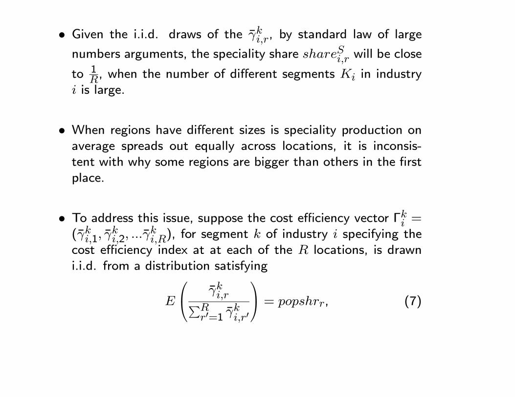
• Given the i.i.d. draws of the , by standard law of large

numbers arguments, the speciality share will be close

to 1, when the number of different segments in industry

is large.

• When regions have different sizes is speciality production onaverage spreads out equally across locations, it is inconsis-tent with why some regions are bigger than others in the firstplace.

• To address this issue, suppose the cost efficiency vector Γ =(1

2

), for segment of industry specifying the

cost efficiency index at at each of the locations, is drawni.i.d. from a distribution satisfying

⎛⎝ P0=1

0

⎞⎠ = , (7)

Then

≈ × . (8)

•

Data

• 1997 Census of Manufactures (CM): Plant level data of theuniverse of plants (sales, location, etc.)

• 1997 Commodity Flow Survey (CFS): Sample of Shipments

from a sample of (15,000) plants

— origin and destination and link to CM

— after conditioning on industry and distance, we use 500,000

observations for structural estimates

Data Selections

• Industry defined at 6-digit NAICS level (North American In-dustry Classification System). Pick 172 (out of 473) indus-

tries where demand approximately follows population

• is population share

• Locations defined at level of Bureau of Economic AnalysisEconomic Area

— = 177

— Based on MSAs, except rural counties get included in the

partition

Seven Industries that Get Extra Attention

• 1997 changed from SIC to NAICS, a ”production based sys-tem.” Plants using the “same production technology” groupedin the same industry

• SIC system

— did this sometimes (sugar from beets and from cane dif-ferent industries)

— “missed” other times, some chocolate factories, wood fur-niture stores, etc. placed in retail under SIC

• 1997 micro data, for these seven industries for each planthave NAICS and SIC. Use this to classify plants as R or Mdepending on SIC. Take R as a proxy for speciality.

Quantitative Analysis

• Model of distance adjustment for ,

ln 0◦ = −loglog ln 0◦

which yields a constant distance elasticity loglog . The second

is a semi-log specification,

ln 0◦ = −semi,1 0◦ − semi,2 (0◦)

2 ,

• First-stage estimates: Constrained model with only primarysegment (one segment model)

— Pick and Γ = (1 2 177) to:

∗ fit sales distribution across locations perfectly (have theuniverse). Use iterative procedure to back out Γ.

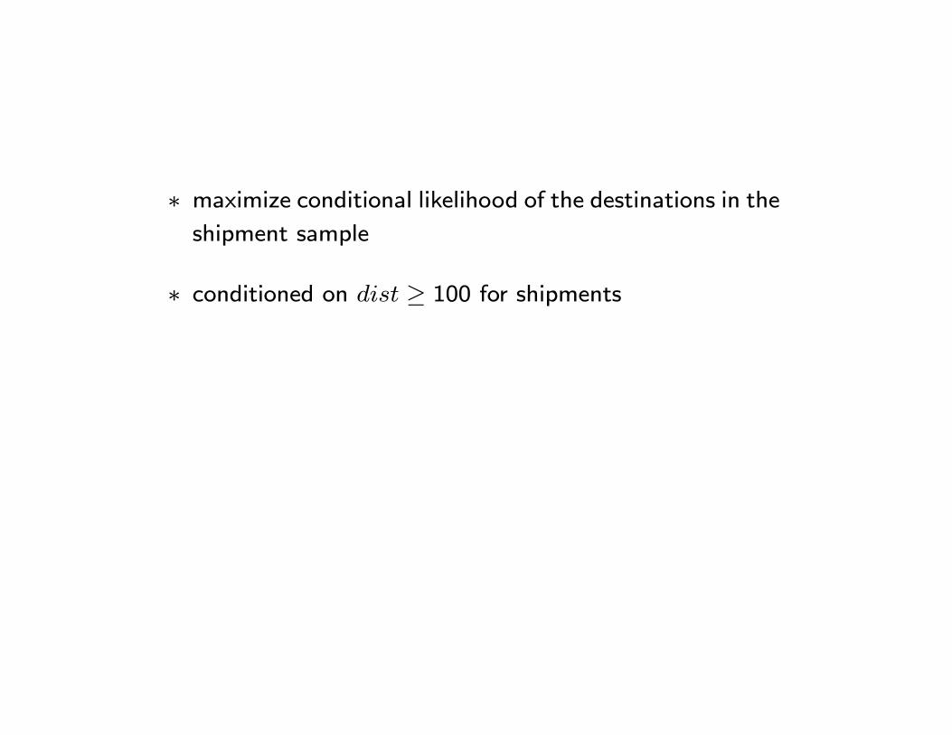
∗ maximize conditional likelihood of the destinations in theshipment sample

∗ conditioned on ≥ 100 for shipments

• Stage 2: Estimate plant count model

— Baseline estimates, take limit where sales revenue share of

specialty is zero. So and Γ same as for one segment

model of just primary segment.

— Specialty segment still factors into plant counts. Pick and to fit

= (Γ

) + + + , (9)

— Also consider an alternative where make assumptions on

size of speciality plants and difference them out of sales,

with little difference in results.

Plan

• Compare

— Estimated industry model with only primary segment

— Estimated industry modwl with specialty segment

• Examine plant size/geographic concentration relationship

• Examine effect of China surge

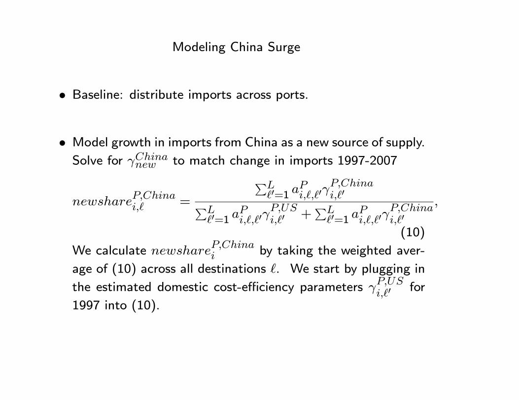
Modeling China Surge

• Baseline: distribute imports across ports.

• Model growth in imports from China as a new source of supply.Solve for to match change in imports 1997-2007

=

P0=1

0

0P

0=1 0

0 +

P0=1

0

0

(10)

We calculate by taking the weighted aver-

age of (10) across all destinations . We start by plugging in

the estimated domestic cost-efficiency parameters 0 for

1997 into (10).

• Next let

= × ,

where is the share in the 2007 data of man-ufacturing imports from China going through customs at loca-tion . We solve for the scaler so that the implied

value of equals the China new-import sharefor industry .

• Stochastic transition of cost efficiency. To explicitly take intoaccount this force, we employ the following procedure. Westart with those 88 industries in the bottom category of Table8 for which the new China share is zero. We take make agrid of the cost efficiencies in 1997 and 2007 and estimate astochastic transition process for the cost efficiencies over thegrid. We then assume the same transition matrix applies forthe other industries, and run 10,000 different simulations, tak-ing averages over simulations for each location and industry.