Embed Size (px)
Citation preview

Band 82
Tobias Schnaidt
Bewertung und Finanzierung in der Immobilien-projektentwicklung
Schriften
zu Immobilienökonomie
und Immobilienrecht
Herausgeber:
IREIBS International Real Estate Business School
Prof. Dr. Sven Bienert
Prof. Dr. Stephan Bone-Winkel
Prof. Dr. Kristof Dascher
Prof. Dr. Dr. Herbert Grziwotz
Prof. Dr. Tobias Just
Prof. Gabriel Lee, Ph. D.
Prof. Dr. Kurt Klein
Prof. Dr. Jürgen Kühling, LL.M.
Prof. Dr. Gerrit Manssen
Prof. Dr. Dr. h.c. Joachim Möller
Prof. Dr. Karl-Werner Schulte HonRICS
Prof. Dr. Wolfgang Schäfers
Prof. Dr. Steffen Sebastian
Prof. Dr. Wolfgang Servatius
Prof. Dr. Frank Stellmann
Prof. Dr. Martin Wentz


I Inhaltsverzeichnis
Inhaltsverzeichnis
Inhaltsverzeichnis ....................................................................................................... I
Abkürzungsverzeichnis Kapitel 1 ................................................................................ III
Abkürzungsverzeichnis Kapitel 2 ................................................................................ III
Abkürzungsverzeichnis Kapitel 3 ................................................................................ III
Abkürzungsverzeichnis Kapitel 4 ............................................................................... IV
Symbolverzeichnis .................................................................................................... VI
1 Einleitung ........................................................................................................... 1
2 German valuation: Review of methods and legal framework .............................. 6
2.1 Introduction ............................................................................................... 6
2.2 Legal sources and fields of application ........................................................ 8
2.3 Transparency of information ....................................................................... 9
2.4 Value definitions: market value ................................................................. 10
2.5 Value definitions mortgage value .............................................................. 11
2.6 Definitions of rents ................................................................................... 11
2.7 Methods ................................................................................................... 13
2.7.1 Cost approach ................................................................................... 13
2.7.2 Comparative method ......................................................................... 14
2.7.3 Capitalisation approach ..................................................................... 16
2.7.4 Formulation and function of the rate of capitalisation ........................ 17
2.7.5 DCF Method ...................................................................................... 19
2.8 Conclusion ................................................................................................ 20
3 Alternative Immobilienfinanzierung durch Immobilienanleihen - Alternative Real
Estate Financing with Real Estate Bonds .................................................................. 21
3.1 Einleitung ................................................................................................. 21
3.2 Immobilienanleihe .................................................................................... 22
3.3 Gründe für alternative Finanzierungsinstrumente ...................................... 23
3.3.1 Finanzierungssituation in der Immobilienwirtschaft ............................ 23
3.3.2 Regulierungen ................................................................................... 24
3.4 Disintermediation durch Anleihen ............................................................. 26
3.4.1 Grundlegende Einordung ................................................................... 26
3.4.2 Finanzierungskosten mittels Anleihen ................................................ 28
3.5 Emissionsmuster von Immobilienanleihen in der Praxis .............................. 30
II Inhaltsverzeichnis
3.5.1 Theorie, Beschreibung der Datenbasis und der Erhebung ................... 30
3.5.2 Unternehmensfinanzierung mit Immobilienanleihen .......................... 32
3.5.3 Fallbeispiel Bestandfinanzierung ........................................................ 32
3.5.4 Fallbeispiel Projektentwicklung .......................................................... 33
3.5.5 Fallbeispiel Immobilienanleihe im Insolvenzfall ................................... 35
3.6 Fazit ......................................................................................................... 36
4 Real estate development – Risk and Solvency ................................................... 37
4.1 Introduction ............................................................................................. 37
4.2 Literature review....................................................................................... 38
4.3 The model ................................................................................................ 41
4.3.1 Fundamentals of residual valuation.................................................... 41
4.3.2 Setup ................................................................................................ 44
4.3.3 Simulation of Residual and Time: ....................................................... 45
4.3.4 Iteration based quantification ............................................................ 50
4.3.5 Risk analysis and continuation of the iteration ................................... 55
4.4 Case studies ............................................................................................. 55
4.5 Variations of the model: ........................................................................... 67
4.6 Conclusion ............................................................................................... 68
Anhang ................................................................................................................... 69
Zusammenfassung der Emissionen von Immobilienanleihen 2005 bis 2013 ......... 70
Literatur .................................................................................................................. 73
Legal sources ...................................................................................................... 79

III Abkürzungsverzeichnis Kapitel 1
Abkürzungsverzeichnis Kapitel 1
IFRS International Financial Reporting Standards
OMV Open Market Value
RICS Royal Institution of Chartered Surveyors
TEGoVA The European Group of Valuers Associations
Abkürzungsverzeichnis Kapitel 2
BVI Bundesverband Investment und Asset Management
C coefficient
DCF Discounted Cash Flow
ImmoWertV Immobilienwertermittlungsverordnung
IPD International Property Database
IVSC International Valuers Standards Council
LUR Land Use Ratio
M Multiplier
P Sales prices
RN Net revenue
T Remaining lifespan
TC Rate of capitalisation
V Market Value
VS Ground value
Abkürzungsverzeichnis Kapitel 3
BCG Boston Consulting Group
GDV Gesamtverband der Deutschen Wohnungswirtschaft
i Expliziten Kapitalkosten
I Intermediär
KAGB Kapitalanlagegesetzbuch
rf Risikofeier Zins
RZ Risikozuschlag
SchVG Schuldverschreibungsgesetz
TAK Transaktionskosten
IV Abkürzungsverzeichnis Kapitel 4
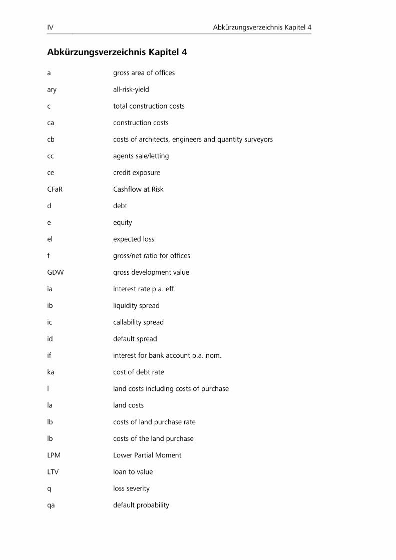
Abkürzungsverzeichnis Kapitel 4
a gross area of offices
ary all-risk-yield
c total construction costs
ca construction costs
cb costs of architects, engineers and quantity surveyors
cc agents sale/letting
ce credit exposure
CFaR Cashflow at Risk
d debt
e equity
el expected loss
f gross/net ratio for offices
GDW gross development value
ia interest rate p.a. eff.
ib liquidity spread
ic callability spread
id default spread
if interest for bank account p.a. nom.
ka cost of debt rate
l land costs including costs of purchase
la land costs
lb costs of land purchase rate
lb costs of the land purchase
LPM Lower Partial Moment
LTV loan to value
q loss severity
qa default probability

V Abkürzungsverzeichnis Kapitel 4
r office rent
s sales price minus cost of selling
s sales price minus cost of selling
t total time
T maximum time
t total time
ta construction time
tb void time
u residual
ul unexpected loss
v total construction cost factor
VaR Value at Risk
y equity yield p.a.
yp years purchase rate
ZRPF Zero Recourse Project Finance

VI Symbolverzeichnis
Symbolverzeichnis
σ Standardabweichung
σ² Varianz
1 Einleitung
1 Einleitung
Die Immobilienprojektentwicklung ist ein komplexer Prozess, der mit Vielzahl von
Entscheidungen verbunden ist, die weitreichende Konsequenzen haben.
Die Entscheidung für oder gegen ein Projekt hängt maßgeblich vom Wert nach der
Entwicklung (Verkaufspreis), dem Wert vor der Entwicklung (Einkaufspreis) den (Hers-
tellungs-)Kosten und damit dem Gewinn des Projekts zusammen. Die in den (Herstel-
lungs-)Kosten enthaltenen Kosten der Finanzierung sind dabei von der Art der Finan-
zierung abhängig: Sie kann Einfluss auf die Verteilung von Risiko und Rendite haben.
Vorliegende Dissertation setzt sich mit den Aspekten Bewertung, Finanzierungsalter-
nativen und quantitativem Risikomanagement auseinander
Den ersten Teil der Dissertation bildet der Aufsatz „German valuation: review of me-
thods and legal framework“, der in Zusammenarbeit von Prof. Dr. Steffen Sebastian
und Tobias Schnaidt entstanden und im 2012 Journal of Property Investment and Fi-
nance veröffentlicht wurde.
Motiviert ist der Aufsatz durch die seit einigen Jahrzehnten laufenden Diskussionen
über die Präzision der deutschen Immobilienbewertungsmethoden, die insbesondere
den Vergleich mit den angelsächsischen oder britischen Verfahren suchen. Als Haupt-
kritikpunkt werden die zu statische Anpassung und eine damit einhergehende man-
gelhafte Anpassung an die aktuellen Marktwerte genannt, die zu einer unsachgemä-
ße Glättung führen können.1 Die britischen Bewertungsmethoden werden hingegen
als dynamisch und marktkonform wahrgenommen. Die Debatte hat insbesondere
dadurch an Dynamik gewonnen, dass es zu einem gestiegenen Bedarf an internatio-
nalen Bewertungsstandards gekommen ist. Im Rahmen der europäischen Harmonisie-
rungsbemühungen stellt sich die Frage, ob man das Red Book der Royal Institution of
Chartered Surveyors (RICS), die Empfehlungen der The European Group of Valuers
Associations (TEGoVA) oder doch nationale Standards bei der Immobilienbewertung
zur Anwendung kommen sollen. Grenzübergreifende Investitionen und internationale
Immobilienunternehmen, die sich an die International Financial Reporting Standards
(IFRS) halten müssen, führen auch zu der Frage, ob es einen internationalen Bewer-
tungsstandard gibt, der generell zur Anwendung kommen sollte.
Ziel des Aufsatzes ist zu zeigen, dass die deutsche Bewertungsmethodik nicht wie
häufig behauptet zu Ergebnissen führt, die nicht die aktuellen Marktkonditionen wie-
derspiegeln und massiv geglättet sind. Kritik am deutschen Bewertungssystem kam
insbesondere nach der Krise der Offenen Immobilienfonds 2005/2006 auf.2
Der Kritik der britischen Bewerter entgegnen die deutschen Bewerter, dass die
deutsche Bewertungsmethodik mit ihren Werten, die auf nachhaltig erzielbaren Mie-
1 Vgl. Crosby (2007). 2 Vgl. Gläsner et al. (2010), Weistroffer (2010)
2 Einleitung
ten basiert, die beabsichtigten Ergebnisse liefert und dabei transparenter ist als der
britische Ansatz und somit als überlegen anzusehen ist.
Im Aufsatz werden die deutschen Bewertungsmethoden analysiert und die vorherr-
schenden Unterschiede zu den britischen Bewertungsstandards hervorgehoben. Es
wird gezeigt, dass die vorgestellten Bewertungsmethoden zu vergleichbaren Ergeb-
nissen führen und auch, dass signifikante Unterschiede zu den britischen Bewer-
tungsstandards nicht der Hauptfaktor für die Glättung in der Bewertung sind. Die ob-
servierten empirischen Phänomene müssen mindestens ergänzende Ursachen haben
und somit können die deutschen Bewertungsverfahren hierfür nicht verantwortlich
gemacht werden.
Verkehrs-, Beleihungs- und Residualwerte sind maßgebliche Kennzahlen zur Ent-
scheidungsfindung in der Immobilienprojektentwicklung. Neben der Investitionsent-
scheidung sind diese natürlich auch maßgeblich für die Entscheidungsfindung in der
Finanzierung von Projektentwicklungen.
Als zweiter Teil geht der Aufsatz „Alternative Immobilienfinanzierung durch Immobi-
lienanleihen“, der in Zusammenarbeit von Tobias Schnaidt und
Prof. Dr. Steffen Sebastian entstanden ist, in die Dissertation ein. Der Aufsatz ist 2014
in der Zeitschrift Betriebswirtschaftliche Forschung und Praxis erschienen und fokus-
siert die Immobilienanleihen und deren Bedeutung für die Unternehmens- und Im-
mobilienfinanzierung.
Er ist motiviert durch die Rückläufigkeit des Volumens der bankbasierten gewerbli-
chen Immobilienfinanzierung im Zuge der Weltfinanzkrise in Deutschland.3 Die Regu-
lierung nach Basel III stellt erweiterte Anforderungen an die Eigenkapitalausstattung
der Banken und kann daher einen weiteren Rückgang verursachen.4 Noch im Jahr
2012 wurde in einer Vielzahl von Berichten postuliert, dass insbesondere für Immobi-
lienfinanzierungen Finanzierungslücken bestehen.5 Nach aktuellen Studien ist bislang
davon auszugehen, dass in Deutschland alternative Anbieter (Nichtbanken) den
Rückgang der bankbasierten Finanzierung kompensieren konnten.6 Für den von Ban-
ken dominierten deutschen Immobilienfinanzierungsmarkt wird zukünftig erwartet,
dass der Anteil alternativer Anbieter weiter steigt. Neben den Versicherern, welche
selbst durch die anstehenden Regulierungen nach Solvency II in ihrer Anlageentschei-
dung beeinflusst werden,7 und Kreditfonds (Debt Fonds)
8 werden auch „Immobilien-
anleihen“ genannt. Zudem sind viele Anleger aufgrund des aktuellen niedrigen Zins-
niveaus auf der Suche nach alternativen Anlagemöglichkeiten mit höheren Renditen.
3 Vgl. Hesse/Just (2013), S. 6. 4 Vgl. Graalmann (2011), S. 15. 5 Vgl. Ahlswede/Just (2010), S. 17, Almond (2012), S. 7, Haugwitz (2012), Kat-zung/Schuhmacher (2012). 6 Vgl. Almond/Vrensen (2013), S.1 ff. 7 Vgl. Rehkugler/Schindler (2012). 8 Zu Debt Fonds vgl. Thomesczek (2012).

3 Einleitung
Insbesondere in 2013 lässt sich bei Immobilienanleihen eine Zunahme von Emissionen
beobachten.9
Diese Form der Disintermediation wird auf ihre Zweckdienlichkeit für Anleger und
Anbieter untersucht. Entsprechend der relativ geringen Bedeutung von Immobilienan-
leihen und der schwierigen Abgrenzung zu Mittelstandsanleihen ohne Immobilienbe-
zug existiert bislang keine Marktübersicht zu Immobilienanleihen. Der vorliegende
Beitrag konsolidiert die verfügbaren Daten zu Emissionen von Immobilienanleihen für
2005 bis 2013.
Im Ergebnis induzieren Basel III und Solvency II eine höhere Attraktivität der Alternati-
ven zur bankbasierten Immobilienfinanzierung. Weiterhin ist in Anbetracht des ak-
tuellen Niedrigzinsumfelds und des zunehmenden Margendrucks aus Sicht der Anle-
ger die höhere Rendite ein wesentliches Argument für die Vorteilhaftigkeit von Im-
mobilienanleihen. Anleihen können für die Immobilienfinanzierung eine potentielle
Alternative darstellen. Welche Bedeutung sie aktuell und in Zukunft haben werden,
muss nicht zuletzt aufgrund der unzureichenden Datenbasis offen bleiben. Vieles
spricht dafür, dass es sich auch weiterhin um ein Nischenprodukt handeln wird.
Maßgebliches Kriterium für den Erfolg ist die Frage, ob die Finanzierungskosten bei
Modellen mit Anleihen einem Wirtschaftlichkeitsvergleich mit anderen Alternativen
standhalten. Aus der Sicht der Emittenten von Immobilienanleihen besteht die Vor-
teilhaftigkeit von Immobiliendarlehen darin, durch die Elimination eines Intermediärs
zu günstigeren Finanzierungskosten zu kommen.10
In der Vergangenheit wurden
auch Anleihen zu sehr günstigen Konditionen ausgegeben, obwohl die emittierenden
Unternehmen keine ausreichende Bonität für ein Bankdarlehen ausweisen konnten.
Unter dem Aspekt des Anlegerschutzes ist dies bedenklich.11
Um Finanzierungsalternativen vergleichen zu können, muss man auf geeignete Daten
zurückgreifen können oder die Kosten einer Finanzierung selbst auf Basis der sonst
verfügbaren Daten ermitteln.
Im dritten Teil wird ein quantitatives Bewertungs- und Entscheidungsmodell für das
Risikomanagement eines Trader-Developers vorgestellt. Hier wird die Möglichkeit ge-
geben, Einflüsse verschiedener Finanzierungsarten und entsprechender Risiko- und
Renditeverteilungen zu analysieren.
Die ursprüngliche Entscheidung für ein Entwicklungsprojekt ist schwierig. Transakti-
onskosten sind hoch und das Ergebnis des Projekts ist unsicher. Geht man von einer
Zero-Recourse Projektfinanzierung aus, kann nur das fertiggestellte Projekt eine un-
komplizierte Rückzahlung des eingesetzten Kapitals gewährleisten. Das führt dazu,
dass die Sicherstellung der Liquidität des Entwicklers bis zur Fertigstellung von höch-
ster Wichtigkeit ist.
9 Vgl. Katzung (2013). 10 Für Mittelstandanleihen ohne Immobilienbezug vgl. Horsch/Sturm (2007). 11 Vgl. Katzung (2013).

4 Einleitung
Die eingegangenen Risiken sollten sich in der Finanzierungsstruktur wiederfinden und
schlussendlich durch eine abwägende Betrachtung der möglichen Projektszenarien zu
einem nachvollziehbaren Kaufpreisangebot führen, dass ein angemessenes Risiko-
und Renditeprofil für alle involvierten Parteien zur Folge hat.
Bereits MacFarlane (1995) beschrieb das Problem von Immobilienprojektentwicklern,
das eigene Risiko zu unterschätzen und aufgrund dessen eine zu geringe Rendite an-
zustreben. Eine derartige langfristige Einstellung führt unausweichlich zu einem De-
saster, insbesondere wenn der Entwickler ein Portfolio ähnlicher Projekte und einen
hohen Fremdkapitaleinsatz hat. Weiterhin identifizierte er das Problem, dass erwarte-
te Gewinne in die Finanzierung von späteren Projektentwicklungen eingerechnet
werden, ohne, dass diese gegen etwaige Differenzen im Ergebnis abgesichert sind.
Diese Herangehensweise sei aber für typisch für Immobilienprojektentwickler, die am
Ende eines Immobilienzyklus in die Insolvenz geraten.
Atherton et al. (2008) stellen fest, dass eine Unterschätzung des Risikos zu einer
Überschätzung des Wertes eines Objektes führt und es damit zu einem überhöhten
Kaufangebot des Entwicklungsprojektes kommt.12 Sie weisen darauf hin, dass simula-
tionsbasierte Vorhersagemodelle helfen, die wichtigsten Variablen und den mögli-
chen Einfluss des Entwicklers zu identifizieren. I. d. R. ist die maßgebliche Variable der
Kaufpreisfaktor bzw. der Liegenschaftszins13 zum Zeitpunkt der Fertigstellung oder
Vermietung ist. Dies jedoch ist die Variable auf die der Entwickler den wenigsten Ein-
fluss hat. Obwohl sie erwarten, dass finale Entscheidungen auf Basis gegenwärtiger
Annahmen getroffen werden, glauben Sie, dass eine solche Analyse eine bessere Ent-
scheidung ermöglicht, da unter Berücksichtigung der möglichen Wertschwankungen
die Risikokomponente besser verstanden wird.
Als Methode zur Quantifizierung von Risiken und Renditen wird ein Residualwertver-
fahren eingeführt, dass auf einer Monte Carlo Simulation basiert. Die aus den simu-
lierten Eingangsvariablen hervorgehenden Residuen, die im Wesentlichen aus Ver-
kaufspreis, den Herstellungskosten ohne Finanzierungskosten sowie Bau- und Leers-
tandszeit basieren, werden anschließend mit einem Risikoanaylsetool verbunden. Ite-
rativ werden dann die Anteile von Fremd- und Eigenkapital, die Höhe der Risikoauf-
schläge auf den Fremdkapitalbasiszinssatz und das Risiko-/Renditeprofil des Eigenka-
pitals bestimmt. Dies geschieht beispielhaft mit einer gewählten Ausfallwahrschein-
lichkeit und einem Kaufpreisangebot, das solange angepasst wird, bis das Rendite-
/Risikoprofil den Anforderungen des Entwicklers genügt.
Der vorliegende Aufsatz kann den Verantwortlichen in der Immobilienprojektentwick-
lung helfen, ihre gegenwärtigen Instrumente zur Entscheidungsfindung zu verbes-
sern. Der Fokus liegt hierbei auf Zero-Recourse Projektfinanzierung von Trader-
Developern. Das vorgestellte Modell last sich in verschiedene Richtungen erweitern
12 What should lead on the short run to the fact that the sites are sold to the worst develop-er. 13 ARY All risk yield und YP years purchase

5 Einleitung
und kann helfen verschiedene Finanzierungsformen zu analysieren und zu verglei-
chen. Auch im laufenden Projektentwicklungsprozess kann es genutzt werden, um
nach Realisation von Werten die Risiken und Renditen zu quantifizieren. Sollte es zu
ungünstigen Bedingungen kommen, die die Liquidität gefährden, können so frühzei-
tig Gegenmaßnahmen ergriffen werden, sofern dies im gemeinsamen Interesse der
beteiligten Parteien ist.
6 German valuation: Review of methods and legal framework
2 German valuation: Review of methods and legal frame-
work
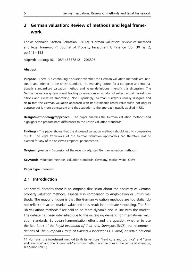
Tobias Schnaidt, Steffen Sebastian, (2012) "German valuation: review of methods
and legal framework", Journal of Property Investment & Finance, Vol. 30 Iss: 2,
pp.145 - 158
http://dx.doi.org/10.1108/14635781211206896
Abstract
Purpose - There is a continuing discussion whether the German valuation methods are inac-
curate and inferior to the British standard. The enduring efforts for a European and interna-
tionally standardised valuation method and value definitions intensify this discussion. The
German valuation system is said leading to valuations which do not reflect actual market con-
ditions and excessive smoothing. Not surprisingly, German surveyors usually disagree and
claim that the German valuation approach with its sustainable rental value fulfils not only its
purpose but is more transparent and thus superior to the approach usually applied in UK.
Design/methodology/approach - The paper analyses the German valuation methods and
highlights the predominant differences to the British valuation standards.
Findings - The paper shows that the discussed valuation methods should lead to comparable
results. The legal framework of the German valuation approaches can therefore not be
blamed for any of the observed empirical phenomenon.
Originality/value – Discussion of the recently adjusted German valuation methods.
Keywords: valuation methods, valuation standards, Germany, market value, OMV
Paper type - Research
2.1 Introduction
For several decades there is an ongoing discussion about the accuracy of German
property valuation methods, especially in comparison to Anglo-Saxon or British me-
thods. The mayor criticism is that the German valuation methods are too static, do
not reflect the actual market value and thus result in inordinate smoothing. The Brit-
ish valuations methods14 are said to be more dynamic and in line with the market.
The debate has been intensified due to the increasing demand for international valu-
ation standards, European harmonisation efforts and the question whether to use
the Red Book of the Royal Institution of Chartered Surveyors (RICS), the recommen-
dations of The European Group of Valuers Associations (TEGoVA) or retain national 14 Normally, the investment method (with its versions “hard core and top slice” and “term and reversion” and the Discounted-Cash-Flow method are the ones in the centre of attention, see Simon (2006).
7 German valuation: Review of methods and legal framework
standards. Cross-border investments and international real estate companies which
need to apply International Financial Reporting Standards (IFRS) lead to the question
whether there is an international valuation standard that can be generally applied or
not.
Criticism on the German valuation system is mainly based upon valuation issues of
the German open ended funds; especially after the crisis in 2005/2006. Crosby
(2007) discusses the valuation process of the German open ended funds and finds
that there is no direct evidence that the property funds were over-valued. However,
he finds that the German valuation process makes an over-valuation in a recession
more likely than in other countries. He further states that the valuations in UK are far
more objective and conceptually correct than in Germany.
Weistroffer (2010) examines empirically the valuation of open ended funds and con-
cludes that the valuation values deviated systematically from the prices achieved in
the market and that the fund properties were overvalued in the previous years before
the crisis. The author attributes this result to the smoothing effect of the German
valuation standards as described by Crosby (2007). The author claims that the Ger-
man valuation system is incapable in reflecting a prolonged downswing in the prop-
erty market in valuation values. He argues the supposed market valuations are in fact
influenced by sustainable value concepts similar to mortgage lending valuations. This
explicit critique is based upon the high degree of smoothness in German property
valuations compared to other standards. The author ascertained that this sustainable
long term value model smoothes the peaks and troughs of the real estate market
and fails to bring forth actual market values. Both Crosby (2007) and Weistroffer
(2010) conclude that the German valuation system was a major cause for the open-
ended fund crisis in 2005/2006.
Gläsner et al. (2010) investigate the valuation of German open ended funds of their
properties in Belgium, France, Italy, the Netherlands, Spain and the UK. They could
demonstrate that they differ significantly from that of other European participants,
i.e. IPD. The authors explain that the stability of capital growth results from the influ-
ence made by fund managers towards appraisers. Those findings are said to be in
contrast to the findings of Crosby et al. (2009) that state that open-end funds in the
UK influence appraisers to mark down valuations more quickly in times of bearish
markets. While Crosby found that UK fund managers strive to quickly mark to mar-
ket, Gläsner et al. find that German fund managers have an interest in stabilising and
smoothing value changes.
In this article, we illustrate the main characteristics of the German valuation stan-
dards and examine whether their methodology is the source of the observed effects
on the German property markets. We find that despite significant differences to the
British valuation standards the methodology on its own cannot be the main factor of
8 German valuation: Review of methods and legal framework
appraisal smoothing. The reasons for the observed empirical phenomenon must have
at least additional causes.
Altmeppen and Brauer (2009) expressed the opinion that is virtually essential to hide
extreme over- or undervaluation of active markets. It would contradict the fair value
concept to appraise a profitable property with a considerable discount in a downturn
of the market. A fair valuation that is worthy of the name should always move mod-
erately and avoid extreme valuations.
Other objections come from practitioners who disregard the German valuation sys-
tem as cumbersome and inefficient (see Zurhorst 1999; see also Morgan and Harrop
1991). As a response German property surveyors criticised this negative view (Mo-
shammer et al. 2000). They reject conclusions that German methods lead to biased
results and that market and object specific circumstances are not taken into account.
Moreover, the surveyors highlight the more explicit consideration of building depre-
ciation. Support for the German valuation standard also comes from Simon (2006),
who rejects the criticism that the German capitalisation method is generally not it
line with the market and too static. He argues that the method itself is not the deci-
sive factor but the objective and justifiable derivation of the market value. Further-
more, the author states that the Anglo-Saxon core & top slice and term & reversion
methods are also known in Germany and that the German capitalisation method cor-
responds with the capitalisation method on basis of the overall capitalisation rate.
The view that German valuation methods are conceptually consistent with methods
used in the UK and internationally is also expressed by Downie et al. (1996). Howev-
er, the authors argue that the application of the methods differs fundamentally.
Most German property surveyors follow strict valuation procedures due to the com-
prehensive codification of valuation techniques in Germany (see Horn 2003).
MacParland et al. (2002) conducted a survey among property valuers in Sweden, the
Netherlands, Germany and France. The results of the survey indicate that no individ-
ual technique is used throughout the four countries and that Germany valuers prefer
the capitalisation method. The arguments for the capitalisation method are the easy
implementation and low complexity in comparison to the DCF method. Furthermore,
German valuers argue that the capitalisation method is said to be the most transpa-
rent due to inadequate market information in Germany.
2.2 Legal sources and fields of application
Today’s regulations first originated from the General Court Ordinance for the Prus-
sian States of 1793. These rules were constantly revised and improved before finally
being grouped together under Prussian law for the Valuations Agency of the 8th
June 1918, the law on which today’s regulations are essentially based. The complete
liberalisation of property prices, which occurred belatedly in 1960 after the price
freeze of 1936, gave rise to the new regulations. It responded to the need for creat-
9 German valuation: Review of methods and legal framework
ing a certain transparency in the property market, something which had not existed
previously, and for protecting sellers and buyers alike against injustices suffered due
to lack of information. It was far from a desire to exert a State influence on price de-
velopments again: essentially it was a question of wanting clarification in order to
restrict extreme fluctuations in property cycles.
It is in this context that property valuation rights were established in paragraphs 192
to 199 of the Construction Code (Baugesetzbuch). This contains the essential ele-
ments regarding the creation of local Committees of valuers (Örtliche Gutachte-
rausschüsse), their remit and the general definition of market value. This code
authorises the federal government to issue decrees for unifying the principles of for-
mulation for the market value, which was done with the Valuation Decree, revised in
1988 and 1997, whereas the Länder (German states) have the capacity to define the
conditions of constitution of the Committees of valuers and their remit. After a long
debate a new legislation, the Property Valuation Decree (ImmoWertV) came recently
into force on July 1st, 2010 replacing the Valuation Decree of 1988.
According to the code of construction, the Property Valuation Decree is the legal
framework applied for all transactions with public bodies and for compensation in
cases of expropriation. Moreover, the agency for monitoring insurance companies
clearly indicated that only the by revenue method in accordance with the Valuation
Decree of 1988 is permitted (it is mandatory for any buildings acquired by an insur-
ance company to be valued before purchase). In principle, in all other circums-
tances it is not mandatory to use the legal framework of valuation. But in praxis all
property valuations in Germany are based solely on this legal framework and only
methods of the Property Value Decree are applied. For example, the law on invest-
ment companies (Investmentgesetz) require that properties held by a property mu-
tual fund must be valued on the occasion of purchase and sale, and at least every
twelve months during the period of ownership. Even though in this instance the
valuers in charge of the funds are free to choose their method, they almost exclu-
sively apply the capitalisation method in accordance with the (Property) Valuation
Decree.
2.3 Transparency of information
Solicitors are obliged to transmit to the local committees a copy of the contract for
each property transaction. If this involves a rented building, the solicitor must also
specify the gross rent. Thus the committee has the information on all the transac-
tions which come under his jurisdiction. The committee also has the right to re-
quest supplementary information from the proprietor as well as from the occupant
of the building. The State agencies and courts are supposed to help the committee
in carrying out its functions. For reasons of confidentiality, the tax office cannot be
involved in this assistance. So in theory 100% percent of all transactions are regis-
10 German valuation: Review of methods and legal framework
tered and detailed information can be demanded from the market participants. Un-
fortunately, decentralisation leads to different levels of professionalism among local
committee and data privacy protection does the rest to avoid that the German
market is not as transparent as it could be.
The Committee constructs a database on the sales prices from the information ga-
thered. Its main task is to draw key figures from this, such as price development in-
dexes. The figures are published or made accessible to the public, whilst the data-
bases themselves remain strictly confidential. Nevertheless, any valuer tasked with
carrying out a valuation can request information which is absolutely necessary for
his valuation but still information may only be communicated without the name of
the proprietors being divulged. The exact extent of anonymity varies according to
the Länder.
2.4 Value definitions: market value
In Germany the market value is defined according to paragraph 194 of the Con-
struction Code as: "... the price which may be achieved under regular trading con-
ditions depending on the legal circumstances and characteristics, depending on
the general nature and the site of the land [...] without regard to any exceptional
or personal circumstances". Legislation interprets this definition by establishing that
the market value is the price which would "probably" be achieved under normal
conditions (the vendor is willing to sell, competent to sell, etc.), which means the
most probable value and which lies at around the average level of potential values
(see Thomas 1995). In the course of the revision of the Valuation Decree of 1988
the term “Verkehrswert” was changed towards “Marktwert”, taking up the rec-
ommendations of the International Valuation Standards Council (IVCS). Both terms
would translate by market value.
These concepts clearly differ from the approach of British valuers who defined un-
til 2003 the open market value (OMV) as the “best price”. In the course of the
harmonization of valuation standards the RICS have replaced the OMV definition
with the definition of the IVSC. The RICS Market value is now defined as the “es-
timated amount for which a property should exchange on the date of valuation
between a willing buyer and a willing seller in an arm’s length transaction after
proper marketing wherein the parties have acted knowledgeably, prudently and
without compulsion.” (French 2003; Mansfeld and Lorenz 2004).
For Germany, Simon (2006) basically interprets the IVSC definition of value as the
price of transactions of comparable properties. According to this interpretation the
German market value has always been sufficient to the definition of the IVSC. Mans-
field and Lorenz (2004) disagree: “Starting from a base where the definitions of the
values are very similar we have to take a look on the main differences that persist.”
11 German valuation: Review of methods and legal framework
The main issue to which Mansfield and Lorenz (2004) refer is their interpretation of
the value. They still see the German market value as an average price of normal busi-
ness dealings and the British market value as the price of best use.
As previously used definitions have not been wrong but only less harmonized and
maybe less clear it is highly questionable if these small differences both between
market value and open market value and German and UK definitions can explain
large if any differences in valuation results.
2.5 Value definitions mortgage value
It is appropriate to present shortly the German concept of mortgage value (Belei-
hungswert) because a large number of valuations are used in determining this value.
Paragraph 16 of the mortgage banks act (Pfandbriefgesetz) defines this value in the
following way:
"The value which is assumed for the loan security must not be greater than the mar-
ket value determined by a cautious formulation […]. In determining this value, only
the durable characteristics of the property and the revenue that the property can
guarantee for each proprietor through correct use may be taken into account".
In practice, the mortgage value is based on the market value reduced by certain al-
lowances against the net revenue; for example between 10 and 30 % for residential
buildings, and 15 to 40 % for offices and commercial premises depending on the
risk. The cautious nature of this approach is seen in particular by the need to antic-
ipate future developments in the property market.
2.6 Definitions of rents
One major issue in the German valuation system is the definition of rents. The Valua-
tion Decree 1988 states that the basis of the estimation with a capitalisation ap-
proach is the “sustainable annual net return”. The net return is further defined as the
difference between the sustainable annual gross return and the sustainable annual
charges.
This definition is cause for various misunderstandings both within German valuers as
well as foreign experts. Frequently this definition has been understood as an average
of the rental value over several years. For example, the spokesman of the German
Federal Association of Investment and Asset Management Companies (BVI), Andreas
Fink was cited saying that future down- and upwards cycles have only limited effect.
Valuers state that an engagement in a property market is a long-term sustainable in-
vestment and therefore valuations should be estimated in a long-term context as well
(Haiman 2005). A similar misinterpretation of Kilbinger (2006) is cited in Crosby
(2007).
12 German valuation: Review of methods and legal framework
Is has clearly to be said that all these kind of interpretation of the term “sustainable
rent” from both German and foreign experts are wrong. The German Valuation De-
crees never left any room for calculation averages over several years or cycles. The
stable and sustainable gross revenue strictly means only that the valuer has to verify
that the rent currently set by the contract is consistent with market rents. If there is a
notable difference, he must apply the market rent.15 With other words, while the Brit-
ish expert would start looking at the existing lease contracts and later adjust the val-
ue for over- or underrenting, his German counterpart would start with the market
rent and adjust finally the market value if the actual rent differs from the market rent.
However to determine the actual market rent, the valuer will usually look backward,
i.e. calculate the market rent as an average of rental contracts archived in the past.
Kleiber (2009) describes that valuers often use rental surveys that are based on aver-
ages of the past four years.
The new Property Valuation Decree 2010 takes at long last into account the everlast-
ing misinterpretations and does no longer use the term “sustainable rents and re-
turns” but “rent and returns usual in the market” i.e. market rents. In the official rea-
sons for the new legislation it is furthermore stated that with this change of terms no
change in the meaning is intended. Rents which are usual in the actual market are
said to be sustainable (see ImmoWertV, p. 52).
Then, having duly verified the gross revenue, the valuers deduct the charges which
are not incumbent upon the tenant in order to obtain the net revenue. The use of net
revenue is often criticised for it fluctuates more or less randomly according to the
charges imputed. The gross revenue might be more stable, but it takes less account
of the investor’s viewpoint. In contrast to UK, this might be relevant because the te-
nant does not bear all the charges, especially usually not major maintenance. In Ger-
many, net and gross revenue are thus not almost always substantially different. The
German method avoids this problem by calculating the charges in the same way as
the revenue, which means stable and sustainable charges. Abnormally low or high
charges must not be taken into account. Thus, maintenance charges to be deducted
are not those for one single period. The consistent annual amount required to consti-
tute a sufficient reserve for carrying out future maintenance works for the remaining
life term of the property is calculated. The predictions require a detailed analysis of
expenses from the previous years. The German valuer may also use reliable statistical
data for predicting the charges.
15 If the term of the lease prevents readjustment for a fairly lengthy period, the valuer must take this into account. In this respect the law does not specify anything explicit. In Great Brit-ain, where commercial leases have a term of twenty to twenty-five years and where property cycles have fluctuated more widely, gaps have often found between market rents and the rents established by the contract. Consequently the British valuation experts have developed sophisticated methods in this respect. In Germany commercial leases have usually a term of five to ten years and are indexed to living costs so have almost developed in line with market rents.

13 German valuation: Review of methods and legal framework
It is very interesting in that context that Gläsner at al. (2010) did indeed find a sub-
stantial smoothing effect in German valuations in Q1 2005 to Q1 2008 but the
change in rental values was at least similar within German open ended funds com-
pared to IPD figures. However, the yield shift is said to differ extremely. German
open-end funds do not change the capitalization rates of their foreign investments in
a comparable way to the domestic market participants which leads to the conclusion
that it is not the definition of the sustainable which causes the smoothing. More like-
ly reasons are behavioural issues, i.e. the potential influence of fund managers to
valuers.
2.7 Methods
To put the German approach into context it is helpful to refer to the general valua-
tion framework. We know that there is no "true value", whether this is for a property
investment or for other investments in general. Values can differ according to the ob-
jectives and reasons for the valuation. For example, for a property the value differs
depending on whether it involves valuing either the maximum price at which an in-
vestor is prepared to purchase the property, or the maximum amount of mortgage
that a bank is prepared to grant against the same property. In all cases the aim
should be to use an "objective" method, which means where the theoretic model can
be checked and controlled. The result of such a valuation can only be criticised for
the following reasons:
1. It is felt that the theoretic model is not true to reality.
2. Empirical transition is called into question, especially the assessment of the
parameters.
But a valuer cannot be tasked with arranging an arbitrary valuation.
The federal government specified the formulation techniques in the Valuation De-
cree, where the permitted methods are described in detail. The terminology in the
decree is oriented along the principal approaches which we find in most other coun-
tries:
1. Cost approach (paragraphs 21 to 25);
2. Comparison approach (paragraphs 13and 14)
3. Capitalisation approach (paragraphs 15 to 20) which includes a so-called
“DCF-method“
We are going to critically examine these methods.
2.7.1 Cost approach
In traditional economic writing it has long been claimed that the value of a com-
mercial item is based around what is called its "natural" value. The natural value is
the sum of all the manufacturing costs which are involved in producing the item.
14 German valuation: Review of methods and legal framework
The value of an item will therefore be equal to its replacement cost. The usual crit-
icism for opposing this method does not account for the different possibilities of
use, and in particular future revenue.
In accordance with the Property Valuation Decree of 2010 the cost replacement
method takes into account the actual costs which must be met in order to repro-
duce the same item in its original condition. These costs benefit from deductions
depending on the level of wear and tear and obsolescence. As the actual result
obtained is rarely the market value, the valuer must estimate the necessary allow-
ance in order to adapt it to the market. Given that the cost replacement method
leads to appraisals which are more or less satisfactory, it might only used in Ger-
many when it involves a building used by the proprietor and when no comparable
transaction exists, such as an unusual type of detached house, for example.
2.7.2 Comparative method
The concept of the comparative method indicates that it is possible to segment the
whole market heterogeneously into different categories depending on the factors
which determine the value, in such a way that we then obtain sufficiently homoge-
nous segments. Inside these segments, from the data regarding the transactions we
can determine a representative price from these segments which can be used as a
comparison basis. As far as factors which determine the value are concerned, in
Property Valuation Decree itemises different criteria, amongst which are qualitative
factors (type of use, site) and quantitative factors (age, area, etc.). Normally, separate
segments are not formed for properties which are only distinguished by quantitative
factors such as age or area, because it is felt that it is possible to calculate the impact
of these factors on the value.
However, as it is practically impossible to measure the impact of a qualitative criterion
such as the region, transactions are grouped together by sites of similar quality and
by use (offices, accommodation, etc.). In other words, we wouldn’t compare an of-
fice block in the centre of Berlin with a hotel in Frankfurt, but we would compare
buildings of different age or size located in sites of similar quality in Stuttgart. It is
crucial for the reliability of this method that there are an adequate number of trans-
actions in all segments, that these are not too old and that they are accessible by
means of databases. Only then will the segment prices be representative and trans-
parent. Although in theory all transaction are available in the databases of the local
authorities including not only transaction prices but various information on the prop-
erty, quality and being up-to-date might vary substantially among different communi-
ties. Some are said not even being able to provide yield data (McParland et al: 2002,
p. 134).
But however subtle the segmentation in the market is, the properties in a segment
always remain too heterogeneous to be directly comparable. Adjustments which take
15 German valuation: Review of methods and legal framework
into account the differences are required. One of the main tasks of the local commit-
tee of valuers is therefore to establish reference prices for land for the region under
their responsibility. The technique consists of attributing a reference value to a ficti-
tious land type whose main characteristics give an approximation of the average land
in the sample used. This land type is described with its main characteristics, in par-
ticular its area, its land use ratio, etc. The value is always given for the year end. From
the transactions the committees will fix coefficients which express the variation in
prices according to changes in the main characteristics. In zones where land is al-
ready built on, the Committees must assess the reference price of a fictitious land
type based on the value this land would have if it was not yet built on.
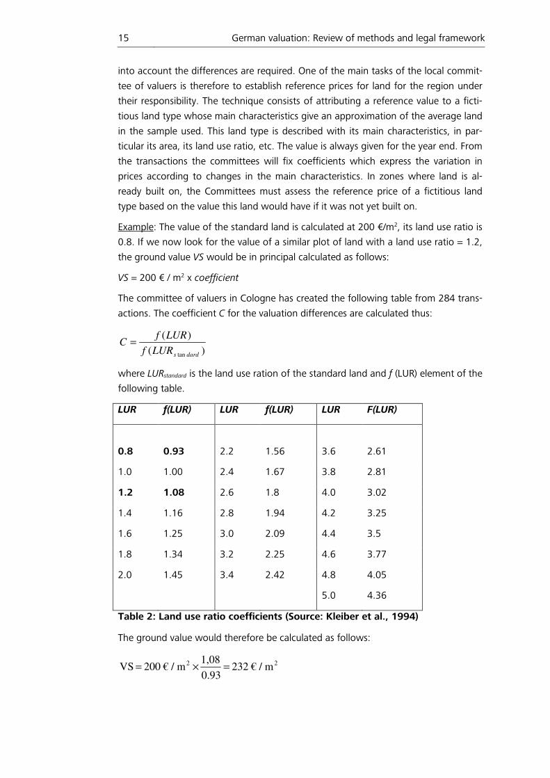
Example: The value of the standard land is calculated at 200 €/m2, its land use ratio is
0.8. If we now look for the value of a similar plot of land with a land use ratio = 1.2,
the ground value VS would be in principal calculated as follows:
VS = 200 € / m2 x coefficient
The committee of valuers in Cologne has created the following table from 284 trans-
actions. The coefficient C for the valuation differences are calculated thus:
)(
)(
tan dardsLURf
LURfC =
where LURstandard is the land use ration of the standard land and f (LUR) element of the
following table.
LUR f(LUR) LUR f(LUR) LUR F(LUR)
0.8 0.93 2.2 1.56 3.6 2.61
1.0 1.00 2.4 1.67 3.8 2.81
1.2 1.08 2.6 1.8 4.0 3.02
1.4 1.16 2.8 1.94 4.2 3.25
1.6 1.25 3.0 2.09 4.4 3.5
1.8 1.34 3.2 2.25 4.6 3.77
2.0 1.45 3.4 2.42 4.8 4.05
5.0 4.36
Table 2: Land use ratio coefficients (Source: Kleiber et al., 1994)
The ground value would therefore be calculated as follows:
22 m / € 232 0.93
1,08 m / € 200 VS =×=
16 German valuation: Review of methods and legal framework
Similar coefficients exist for several other factors such as the area of the plot, the
depth/width ratio etc.
The coefficients defined by the committees allow the valuer to calculate the market
value of a specific plot of land in a manner which is both "objective" and above all
transparent. But despite these solid statistical bases, in some cases market influences
remain which cannot be entirely reproduced by these calculations, especially as in
certain regions the figures are only updated every two years. The valuer is thus enti-
tled to adjust these results depending on his assessment of the current state of the
market.
When the products are too complex, adjustment by coefficients becomes impossible.
It is for this reason that in Germany the application of the method known as the "by
comparison" method only applies to "simple" products such as:
• Standard apartments;
• Common types of buildings intended for use by the proprietors;
• And in particular building plots where the factors which determine the price
can be more easily identified and measured.
2.7.3 Capitalisation approach
The comparison approach is not part of the financial mathematical methods because
essentially it involves only a special comparison method. In fact, the capitalisation ap-
proach does nothing more than compare prices based on their net revenues in as-
suming that the net revenue is the essential factor which determines the price. One
peculiarity of the German method is that initially they assess the market value of the
land separately. This is based on the logic that the ground has an indefinite lifespan
whereas a building has a limited term of use. Even if the separate determination of
the ground value provides in theory more accurate results it is in most cases of little
practical relevance as the result do not alter significantly. Naubereit (2008) examines
IPD data for Germany and finds that the ground value does not require an explicit
provision, while offering added informational value in cases of short remaining build-
ing life.
As far as investment property is concerned, the German method integrates five fac-
tors for value determination (see table 2):
1. The market value of the land.
2. The gross stable and sustainable revenue assuming that there is regular
management.
3. Stable and sustainable charges.
4. The lifespan remaining.
5. The rate of capitalisation.
17 German valuation: Review of methods and legal framework
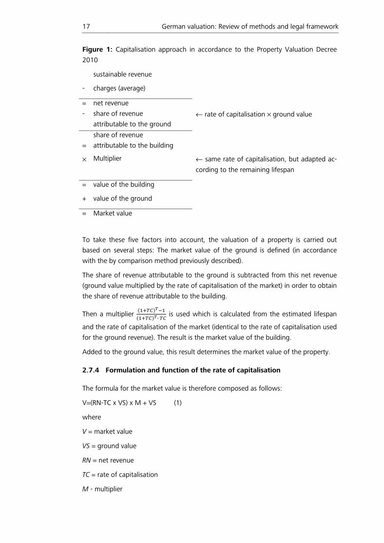
Figure 1: Capitalisation approach in accordance to the Property Valuation Decree
2010
sustainable revenue
- charges (average)
= net revenue
- share of revenue
attributable to the ground
← rate of capitalisation × ground value
=
share of revenue
attributable to the building
× Multiplier ← same rate of capitalisation, but adapted ac-
cording to the remaining lifespan
= value of the building
+ value of the ground
= Market value
To take these five factors into account, the valuation of a property is carried out
based on several steps: The market value of the ground is defined (in accordance
with the by comparison method previously described).
The share of revenue attributable to the ground is subtracted from this net revenue
(ground value multiplied by the rate of capitalisation of the market) in order to obtain
the share of revenue attributable to the building.
Then a multiplier ���������
�������· �� is used which is calculated from the estimated lifespan
and the rate of capitalisation of the market (identical to the rate of capitalisation used
for the ground revenue). The result is the market value of the building.
Added to the ground value, this result determines the market value of the property.
2.7.4 Formulation and function of the rate of capitalisation
The formula for the market value is therefore composed as follows:
V=(RN-TC x VS) x M + VS (1)
where
V = market value
VS = ground value
RN = net revenue
TC = rate of capitalisation
M - multiplier
18 German valuation: Review of methods and legal framework
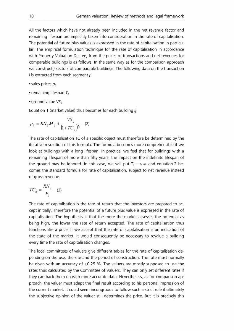
All the factors which have not already been included in the net revenue factor and
remaining lifespan are implicitly taken into consideration in the rate of capitalisation.
The potential of future plus values is expressed in the rate of capitalisation in particu-
lar. The empirical formulation technique for the rate of capitalisation in accordance
with Property Valuation Decree, from the prices of transactions and net revenues for
comparable buildings is as follows: In the same way as for the comparison approach
we construct j sectors of comparable buildings. The following data on the transaction
i is extracted from each segment j:
• sales prices pij.
• remaining lifespan Tij
• ground value VSij
Equation 1 (market value) thus becomes for each building ij:
( ) ijT
ij
ij
ijijij
TC
VSMRNp
++=
1 (2)
The rate of capitalisation TC of a specific object must therefore be determined by the
iterative resolution of this formula. The formula becomes more comprehensible if we
look at buildings with a long lifespan. In practice, we feel that for buildings with a
remaining lifespan of more than fifty years, the impact on the indefinite lifespan of
the ground may be ignored. In this case, we will put Tij —> ∞ and equation 2 be-
comes the standard formula for rate of capitalisation, subject to net revenue instead
of gross revenue:
ij
ij
ijP
RNTC = (3)
The rate of capitalisation is the rate of return that the investors are prepared to ac-
cept initially. Therefore the potential of a future plus value is expressed in the rate of
capitalisation. The hypothesis is that the more the market assesses the potential as
being high, the lower the rate of return accepted. The rate of capitalisation thus
functions like a price. If we accept that the rate of capitalisation is an indication of
the state of the market, it would consequently be necessary to revalue a building
every time the rate of capitalisation changes.
The local committees of valuers give different tables for the rate of capitalisation de-
pending on the use, the site and the period of construction. The rate must normally
be given with an accuracy of ±0.25 %. The valuers are mostly supposed to use the
rates thus calculated by the Committee of Valuers. They can only set different rates if
they can back them up with more accurate data. Nevertheless, as for comparison ap-
proach, the valuer must adapt the final result according to his personal impression of
the current market. It could seem incongruous to follow such a strict rule if ultimately
the subjective opinion of the valuer still determines the price. But it is precisely this
19 German valuation: Review of methods and legal framework
subjectivity that the German methodological framework is trying to reduce to a
minimum. The fact remains that the legislators have always been aware that the
property market, due to the heterogeneous nature of properties, will never be able to
be fully objective which the limit of transparency of any valuation method is. Ulti-
mately, valuations of buildings intended for investment are essentially done using the
capitalisation method (but also involving the ground value obtained through the
comparison method).
Furthermore, with the new regulation of 2010, a simplified version of the capitalisa-
tion approach was introduced which allows to omit the separate valuation of land
and building. We abstain here from a detailed description.
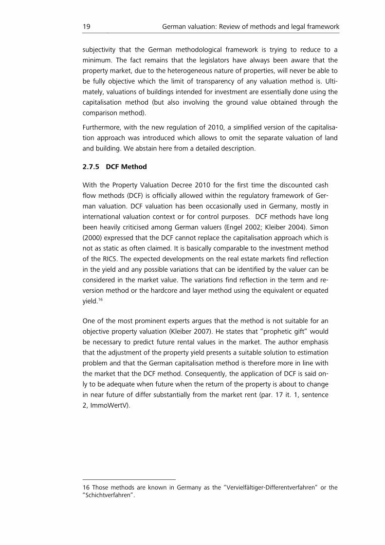
2.7.5 DCF Method
With the Property Valuation Decree 2010 for the first time the discounted cash
flow methods (DCF) is officially allowed within the regulatory framework of Ger-
man valuation. DCF valuation has been occasionally used in Germany, mostly in
international valuation context or for control purposes. DCF methods have long
been heavily criticised among German valuers (Engel 2002; Kleiber 2004). Simon
(2000) expressed that the DCF cannot replace the capitalisation approach which is
not as static as often claimed. It is basically comparable to the investment method
of the RICS. The expected developments on the real estate markets find reflection
in the yield and any possible variations that can be identified by the valuer can be
considered in the market value. The variations find reflection in the term and re-
version method or the hardcore and layer method using the equivalent or equated
yield.16
One of the most prominent experts argues that the method is not suitable for an
objective property valuation (Kleiber 2007). He states that “prophetic gift” would
be necessary to predict future rental values in the market. The author emphasis
that the adjustment of the property yield presents a suitable solution to estimation
problem and that the German capitalisation method is therefore more in line with
the market that the DCF method. Consequently, the application of DCF is said on-
ly to be adequate when future when the return of the property is about to change
in near future of differ substantially from the market rent (par. 17 it. 1, sentence
2, ImmoWertV).
16 Those methods are known in Germany as the “Vervielfältiger-Differentverfahren” or the “Schichtverfahren”.
20 German valuation: Review of methods and legal framework
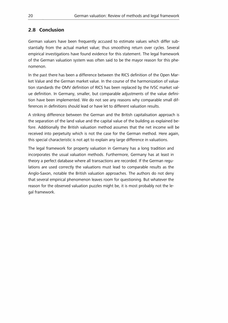
2.8 Conclusion
German valuers have been frequently accused to estimate values which differ sub-
stantially from the actual market value; thus smoothing return over cycles. Several
empirical investigations have found evidence for this statement. The legal framework
of the German valuation system was often said to be the mayor reason for this phe-
nomenon.
In the past there has been a difference between the RICS definition of the Open Mar-
ket Value and the German market value. In the course of the harmonization of valua-
tion standards the OMV definition of RICS has been replaced by the IVSC market val-
ue definition. In Germany, smaller, but comparable adjustments of the value defini-
tion have been implemented. We do not see any reasons why comparable small dif-
ferences in definitions should lead or have let to different valuation results.
A striking difference between the German and the British capitalisation approach is
the separation of the land value and the capital value of the building as explained be-
fore. Additionally the British valuation method assumes that the net income will be
received into perpetuity which is not the case for the German method. Here again,
this special characteristic is not apt to explain any large difference in valuations.
The legal framework for property valuation in Germany has a long tradition and
incorporates the usual valuation methods. Furthermore, Germany has at least in
theory a perfect database where all transactions are recorded. If the German regu-
lations are used correctly the valuations must lead to comparable results as the
Anglo-Saxon, notable the British valuation approaches. The authors do not deny
that several empirical phenomenon leaves room for questioning. But whatever the
reason for the observed valuation puzzles might be, it is most probably not the le-
gal framework.
21 Alternative Immobilienfinanzierung durch Immobilienanleihen - Alternative Real Estate Financing with Real Estate Bonds
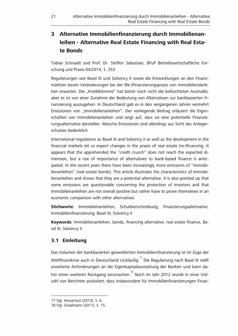
3 Alternative Immobilienfinanzierung durch Immobilienan-
leihen - Alternative Real Estate Financing with Real Esta-
te Bonds
Tobias Schnaidt und Prof. Dr. Steffen Sebastian, BFuP Betriebswirtschaftliche For-
schung und Praxis 04/2014, S. 353
Regulierungen wie Basel III und Solvency II sowie die Entwicklungen an den Finanz-
märkten lassen Veränderungen bei der (Re-)Finanzierungspraxis von Immobiliendarle-
hen erwarten. Die „Kreditklemme“ hat bisher noch nicht die befürchteten Ausmaße,
aber es ist von einer Zunahme der Bedeutung von Alternativen zur bankbasierten Fi-
nanzierung auszugehen. In Deutschland gab es in den vergangenen Jahren vermehrt
Emissionen von „Immobilienanleihen“. Der vorliegende Beitrag erläutert die Eigen-
schaften von Immobilienanleihen und zeigt auf, dass sie eine potentielle Finanzie-
rungsalternative darstellen. Manche Emissionen sind allerdings aus Sicht des Anleger-
schutzes bedenklich.
International regulations as Basel III and Solvency II as well as the development in the
financial markets let us expect changes in the praxis of real estate (re-)financing. It
appears that the apprehended the “credit crunch“ does not reach the expected di-
mension, but a rise of importance of alternatives to bank-based finance is antic-
ipated. In the recent years there have been increasingly more emissions of “Immobi-
lienanleihen” (real estate bonds). This article illustrates the characteristics of Immobi-
lienanleihen and shows that they are a potential alternative. It is also pointed up that
some emissions are questionable concerning the protection of investors and that
Immobilienanleihen are not overall positive but rather have to prove themselves in an
economic comparison with other alternatives.
Stichworte: Immobilienanleihen, Schuldverschreibung, Finanzierungsalternative,
Immobilienfinanzierung, Basel III, Solvency II
Keywords: Immobilienanleihen, bonds, financing alternative, real estate finance, Ba-
sel III, Solvency II
3.1 Einleitung
Das Volumen der bankbasierten gewerblichen Immobilienfinanzierung ist im Zuge der
Weltfinanzkrise auch in Deutschland rückläufig.17
Die Regulierung nach Basel III stellt
erweiterte Anforderungen an die Eigenkapitalausstattung der Banken und kann da-
her einen weiteren Rückgang verursachen.18
Noch im Jahr 2012 wurde in einer Viel-
zahl von Berichten postuliert, dass insbesondere für Immobilienfinanzierungen Finan-
17 Vgl. Hesse/Just (2013), S. 6. 18 Vgl. Graalmann (2011), S. 15.
22 Alternative Immobilienfinanzierung durch Immobilienanleihen - Alternative Real Estate Financing with Real Estate Bonds
zierungslücken bestehen.19
Nach aktuellen Studien ist bislang davon auszugehen,
dass in Deutschland alternative Anbieter (Nichtbanken) den Rückgang der bankba-
sierten Finanzierung kompensieren konnten.20
Für den von Banken dominierten deut-
schen Immobilienfinanzierungsmarkt wird zukünftig erwartet, dass der Anteil alterna-
tiver Anbieter weiter steigt. Neben den Versicherern, welche selbst durch die anste-
henden Regulierungen nach Solvency II in ihrer Anlageentscheidung beeinflusst wer-
den,21
und Kreditfonds (Debt Fonds)22
werden auch „Immobilienanleihen“ genannt.
Zudem sind viele Anleger aufgrund des aktuellen niedrigen Zinsniveaus auf der Suche
nach alternativen Anlagemöglichkeiten mit höheren Renditen. Insbesondere in 2013
lässt sich bei Immobilienanleihen eine Zunahme von Emissionen beobachten.23
Dieser Beitrag fokussiert die Immobilienanleihen und deren Bedeutung für die Unter-
nehmens- und Immobilienfinanzierung. Hierbei wird diese Form der Disintermediation
auf ihre Zweckdienlichkeit für Anleger und Anbieter untersucht. Entsprechend der re-
lativ geringen Bedeutung von Immobilienanleihen und der schwierigen Abgrenzung
zu Mittelstandsanleihen ohne Immobilienbezug existiert bislang keine Marktübersicht
zu Immobilienanleihen. Der vorliegende Beitrag konsolidiert die verfügbaren Daten zu
Emissionen von Immobilienanleihen für 2005 bis 2013.
3.2 Immobilienanleihe
Eine Anleihe ist grundsätzlich eine Darlehensurkunde in Form einer Schuldverschrei-
bung auf den Inhaber gemäß § 793 BGB, durch die der Aussteller zu einer Leistung
an den jeweiligen Inhaber der Urkunde verpflichtet wird. Zudem werden häufig die
Normen des Schuldverschreibungsgesetzes (SchVG)24
zur Anwendung kommen, die
im Wesentlichen Regelungen zur Beschlussfassung der Anleger beinhalten und für
den Fall der Insolvenz des Schuldners eine Sanierung – beispielsweise durch Forde-
rungsverzicht – ermöglichen sollen.25
Gemäß § 1 Abs.1 SchVG erstreckt sich das Ge-
setz für inhaltsgleiche Schuldverschreibungen nach deutschem Recht aus Gesamt-
emissionen.26
Somit ist der maßgebliche Unterschied zu gewöhnlichen Darlehen, dass
bei Anleihen eine Handelbarkeit bereits ohne Einwilligung des Schuldners vorgesehen
ist.
19 Vgl. Ahlswede/Just (2010), S. 17, Almond (2012), S. 7, Haugwitz (2012), Kat-zung/Schuhmacher (2012). 20 Vgl. Almond/Vrensen (2013), S.1 ff. 21 Vgl. Rehkugler/Schindler (2012). 22 Zu Debt Fonds vgl. Thomesczek (2012). 23 Vgl. Katzung (2013). 24 Schuldverschreibungsgesetz (SchVG) vom 31.07.2009. 25 Vgl. Vogel (2013), S. 5f. 26 Nach § 2 Abs.2 SchVG nicht für Schuldverschreibungen nach Pfandbriefgesetz oder der öffentlichen Hand.
23 Alternative Immobilienfinanzierung durch Immobilienanleihen - Alternative Real Estate Financing with Real Estate Bonds
Der Begriff der Immobilienanleihe ist hingegen gesetzlich nicht definiert und wird
entsprechend in Schrifttum und Praxis nicht einheitlich verwendet. Unter Immobilien-
anleihen werden daher grundsätzlich alle Anleihen mit Immobilienbezug verstanden,
sei es in Form einer grundpfandrechtlichen Absicherung oder aufgrund der Zugehö-
rigkeit des Emittenten zur Bau- bzw. Immobilienbranche. Im letzteren Fall kann die
Anleihe auch ungesichert oder nur durch Negativerklärung gesichert sein.27
Sofern Anleihen nicht oder nur nachrangig über Grundpfandrechte besichert werden,
drohen Anleihegläubigern vergleichbar mit Mezzanine-Kreditgebern bei Kreditausfall
der Totalverlust ihrer Einlage. Zudem werden diese Anleihen oftmals nur zur Finanzie-
rung einer oder weniger Immobilien über Objektgesellschaften vergeben und können
ein hohes idiosynkratisches Risiko beinhalten. Somit sind Immobilienanleihen ver-
gleichbar mit einer Fremdkapitalform von Geschlossenen Immobilienfonds. Ebenso
wie diese weisen sie auch den Nachteil einer nur eingeschränkten Handelbarkeit auf.
Während Geschlossene Immobilienfonds durch das im Juli 2013 in Kraft getretene
Kapitalanlagengesetzbuch (KAGB) umfassend reguliert werden, gibt es für Immobi-
lienanleihen keinen vergleichbaren gesetzlichen Rahmen des Anlegerschutzes. Bei-
spielsweise existieren keine Vorschriften für das Verhältnis von Emissionsvolumen zu
Grundstückswert. Bei unbedarften Privatanlegern kann der Begriff Immobilienanleihe
daher eine Sicherheit suggerieren, die tatsächlich nicht gegeben ist.28
Bemerkenswert
ist, dass der Begriff Immobilienanleihe in den Wertpapierprospekten äußerst selten
vertreten ist. In Presse, Veröffentlichungen von Kanzleien und Werbung von Unter-
nehmen findet sich dieser Begriff hingegen vielfach29
. Aus Anlegersicht stellen Immo-
bilienanleihen somit eine grundsätzlich riskante Anleihe mit geringer Liquidität dar.
Entsprechend sollte dies durch eine angemessene Risiko- und Liquiditätsprämie ent-
lohnt werden. Zudem sollten einzelne Immobilienanleihen als undiversifizierte Anla-
geform nur einen geringen Anteil am gesamten Anlagevermögen haben.
3.3 Gründe für alternative Finanzierungsinstrumente
3.3.1 Finanzierungssituation in der Immobilienwirtschaft
In den kommenden Jahren stehen große Volumina von Gewerbeimmobilienfinanzie-
rungen zur Refinanzierung an. Der Markt für Immobilienfinanzierungen in Deutsch-
land ist im Wesentlichen bankenbasiert. Das Angebot von Immobilienfinanzierungen
wird sich durch die anstehenden Regulierungen zur Umsetzung von Basel III jedoch
tendenziell verringern.30
27 Vgl. hierzu die Typisierung von Loritz (2011), S. 15. 28 Vgl. hierzu Alram/Schalast (2009), S.48 im Kontext des zulässigen Wettbewerbs und Irre-führung bzgl. Abgrenzung von Hypothekenanleihe und Hypothekenpfandbrief. 29 z.B. Katzung (2013), Brückner/de Boer (2011), Samonig AG (2011). 30 Vgl. Ahlswede/Just (2010), S. 17.
24 Alternative Immobilienfinanzierung durch Immobilienanleihen - Alternative Real Estate Financing with Real Estate Bonds
Almond (2012) ermittelt für Deutschland eine Finanzierungslücke in den Jahren 2012
und 2013 in Höhe von 19,7 Mrd. Euro. Die weltweite Finanzierungslücke sieht er bei
163,52 Mrd. Euro.31
Nach Volquarts und Radner (2011) werden alternative Finanzie-
rungsformen durch Basel III, auslaufende Immobiliendarlehen und eine stärkere Fo-
kussierung auf riskante Investments (Value-Add) an Bedeutung gewinnen. Insbeson-
dere bei Neudarlehen ab einem Volumen von 50 Mio. Euro gehen Kapitalgeber und -
nehmer von einer Zunahme alternativer Finanzierungsformen aus.32
Hesse und Just
(2013) prognostizieren ebenfalls, dass der Anteil der alternativen Immobilienfinanzie-
rungen zunehmen wird. Sie sehen aber vor allem Versicherungsunternehmen und
CMBS, mit Einschränkungen auch Debt Fonds, als potentielle Alternative.33
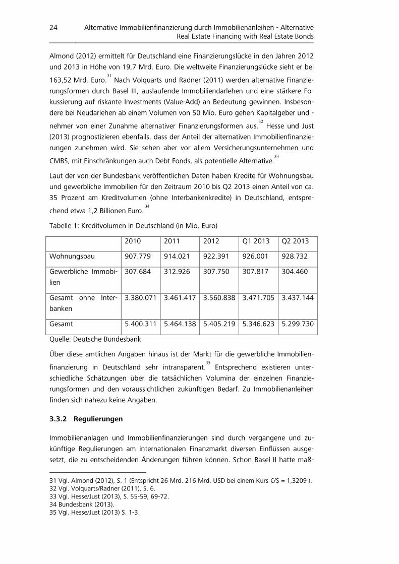
Laut der von der Bundesbank veröffentlichen Daten haben Kredite für Wohnungsbau
und gewerbliche Immobilien für den Zeitraum 2010 bis Q2 2013 einen Anteil von ca.
35 Prozent am Kreditvolumen (ohne Interbankenkredite) in Deutschland, entspre-
chend etwa 1,2 Billionen Euro. 34
Tabelle 1: Kreditvolumen in Deutschland (in Mio. Euro)
2010 2011 2012 Q1 2013 Q2 2013
Wohnungsbau 907.779 914.021 922.391 926.001 928.732
Gewerbliche Immobi-
lien
307.684 312.926 307.750 307.817 304.460
Gesamt ohne Inter-
banken
3.380.071 3.461.417 3.560.838 3.471.705 3.437.144
Gesamt 5.400.311 5.464.138 5.405.219 5.346.623 5.299.730
Quelle: Deutsche Bundesbank
Über diese amtlichen Angaben hinaus ist der Markt für die gewerbliche Immobilien-
finanzierung in Deutschland sehr intransparent.35
Entsprechend existieren unter-
schiedliche Schätzungen über die tatsächlichen Volumina der einzelnen Finanzie-
rungsformen und den voraussichtlichen zukünftigen Bedarf. Zu Immobilienanleihen
finden sich nahezu keine Angaben.
3.3.2 Regulierungen
Immobilienanlagen und Immobilienfinanzierungen sind durch vergangene und zu-
künftige Regulierungen am internationalen Finanzmarkt diversen Einflüssen ausge-
setzt, die zu entscheidenden Änderungen führen können. Schon Basel II hatte maß-
31 Vgl. Almond (2012), S. 1 (Entspricht 26 Mrd. 216 Mrd. USD bei einem Kurs €/$ = 1,3209 ). 32 Vgl. Volquarts/Radner (2011), S. 6. 33 Vgl. Hesse/Just (2013), S. 55-59, 69-72. 34 Bundesbank (2013). 35 Vgl. Hesse/Just (2013) S. 1-3.
25 Alternative Immobilienfinanzierung durch Immobilienanleihen - Alternative Real Estate Financing with Real Estate Bonds
gebliche Auswirkungen auf die Immobilienfinanzierung. Insbesondere bei den Ent-
wicklern stiegen die Kapitalkosten.36
Aktuell stehen Basel III und Solvency II im Vor-
dergrund, die noch nicht abschließend in gültiges Recht umgesetzt sind. Beide Re-
gelwerke sind aktuell Thema einer Reihe von Aufsätzen, die insbesondere auf die zu
erwartenden Wechselwirkungen eingehen und die möglichen Effekte auf Immobilien-
investitionen und -finanzierungen untersuchen. Hughes und Moss (2011) gehen
durch die aktuelle Gestaltung von Solvency II davon aus, dass sich bei den Versiche-
rungen eine Reallokation von direkten Immobilieninvestitionen hin zu Immobilienfi-
nanzierungen einstellen wird, die auf die Höhe der jeweiligen Kapitalunterlegung zu-
rückzuführen ist.37
Darüber hinaus erwarten sie einen Zuwachs der Bedeutung von
Anleihen und eine Steigerung der Fremdkapitalkosten bei abnehmender Verfügbar-
keit.38
Die generelle Attraktivität von Unternehmensanleihen mit gutem Rating wird auch
dadurch steigen, dass Bankanleihen unter den Einflüssen von Basel III und Solvency II
an Attraktivität verlieren. Investitionsentscheidungen von Versicherungen werden
trotz der Regulierungen auch weiterhin maßgeblich von den Zahlungsverpflichtungen
der Versicherer abhängen, aufgrund derer eine Auswahl bezüglich Laufzeit und Cash-
flow eines Investments entscheidend ist.39
Der Gesamtverband der Deutschen Versicherungswirtschaft e.V. (GDV) (2011) sieht
durch die aktuelle Kalibrierung des Spreadrisikos falsche Anreize gesetzt. Diese be-
günstigt die Investition in kurzfristige Anlagen. Für Versicherer, die i.d.R. langfristige
Verbindlichkeiten haben, ergibt sich so eine Durationslücke, die sie verstärkt dem
Zinsänderungsrisiko aussetzt. Auch die momentan noch vorgesehene Konzentration
auf Ratings bei der Kapitalunterlegung von Anlagen stößt beim GDV auf Kritik, der
eine ungerechte Gleichstellung von Pfandbriefen mit AA Rating und anderen Schuld-
titeln sieht.40
Mögliche Anhaltspunkte, um die Effekte durch Regulierungen abzu-
schätzen, liefern Fallbeispiele aus anderen Ländern. An dieser Stelle seien die USA
erwähnt. Hier wurde bereits in den 90er Jahren eine risikobasierte Kapitalunterlegung
für das Minimumsolvenzkapital eingeführt. Für die Versicherer wurden durch die Re-
gulierung CMBS attraktiver als die üblichen Darlehen auf Gewerbeimmobilien.41
Rehkugler und Schindler (2012) sehen zwar die (direkten) Immobilienanlagen in
Deutschland für Versicherer einem Nachteil ausgesetzt, da die geforderte Eigenmit-
telausstattung nicht kongruent mit dem deutschen Immobilienmarkt sei. Die Auswir-
kungen von Solvency II sind noch nicht abschließend zu bewerten, sie sind allerdings
36 Vgl. Pitschke (2004), S. 272 -276. 37 Vgl. Hughes/Moss (2011), S. 19. 38 Vgl. Hughes/Moss (2011), S. 21. 39 Vgl. Zähres (2011), S. 16. 40 Vgl. GDV (2011), S. 1-5. 41 Vgl. Zähres (2011), S. 18.
26 Alternative Immobilienfinanzierung durch Immobilienanleihen - Alternative Real Estate Financing with Real Estate Bonds
konkreter als jene, die durch die Basel III auf die Immobilienwirtschaft zukommen.42
Graalmann (2011) geht davon aus, dass es aufgrund von Basel III zu Kreditverknap-
pung oder einem Anstieg der Kreditkosten kommen wird. Er sieht insbesondere das
risikoarme Immobilienkreditgeschäft benachteiligt.43
Untersuchungen von der Boston Consulting Group (BCG) (2010) und Härle et al.
(2010) lassen hier andere Schlüsse zu. BCG geht von einer leichten Kostenreduktion
von 25 Basispunkten44
bei Hypothekendarlehen aus, Härle et al. dagegen von einer
Steigerung von 25 Basispunkten bei Hypothekendarlehen für Wohnimmobilien und
50 Basispunkten bei sonstigen Hypothekendarlehen. Zusätzlich wird eine Kostenre-
duzierung von 10 Basispunkten bei Unternehmensanleihen und Pfandbriefen erwar-
tet, die mindestens ein AA Rating aufweisen. Für Unternehmensanleihen und Pfand-
briefe mit schlechteren oder gar keinen Ratings sind allerdings Kostensteigerungen
von bis zu 70 Basispunkten zu erwarten.45
3.4 Disintermediation durch Anleihen
3.4.1 Grundlegende Einordung
In ihrem grundlegenden Aufsatz kommen Leland und Pyle (1973) zu dem Schluss,
dass die Existenz von Finanzintermediären durch die traditionellen Modelle der Fi-
nanzmärkte nur unzureichend erklärt wird. Wenn Transaktionskosten unberücksich-
tigt bleiben, finden Kapitalgeber und -nehmer direkt zueinander und die Kosten des
Finanzintermediärs werden gespart. Die in der Realität vorhandenen Transaktionskos-
ten sind ein Argument für Intermediation, aber regelmäßig nicht der alleinige Grund.
Der ursächliche Grund in der Realität liegt in der Informationsasymmetrie.46
Nach
Benston und Smith (1976) sind Transaktionskostenvorteile durch Größeneffekte der
Finanzintermediäre möglich und somit sind diese die maßgebliche Existenzberechti-
gung.47
In der Immobilienwirtschaft kann aufgrund der Heterogenität der gehandelten Güter
davon ausgegangen werden, dass Informationsasymmetrien eine maßgebliche Rolle
spielen und somit eine Kapitalüberlassung verhindern können oder einen direkten
Einfluss auf den Preis der Kapitalüberlassung haben. Entsprechend hat der Kapital-
nehmer eine zusätzliche Prämie zu zahlen, die je nach Informationssymmetrie höher
oder niedriger ausfallen kann.
42 Vgl. Rehkugler/Schindler (2012), S. 18 f. 43 Vgl. Graalmann (2011), S. 15. 44 Vgl. BCG (2010), S. 19. 45 Vgl. Härle et. al (2010), S. 9. 46 Vgl. Leland/Pyle (1977), S. 382 f. Demnach können insbesondere Hypotheken- und Versi-cherungsinformationen, die spezifischer Natur und nicht öffentlich verfügbar sind, nur mit großem Aufwand erlangt werden. 47 Vgl. Benston/Smith (1976), S. 216, 222.
27 Alternative Immobilienfinanzierung durch Immobilienanleihen - Alternative Real Estate Financing with Real Estate Bonds
Die expliziten Kapitalkosten i ergeben sich also aus dem risikofreien Zins rf und dem
Risikozuschlag RZ. Weiterhin sind die Transaktionskosten TAK zu integrieren. Daraus
ergibt sich bei vollständiger Betrachtung eine Vorteilhaftigkeit für den Einsatz eines
Intermediärs I und den Kapitalkosten II sofern gilt:48
i = rf + RZ + TAK > rf + RZI + TAKI = iI (1)
Bei der Bemessung des Risikozuschlag ist festzuhalten, dass ein Intermediär die mög-
lichen Risiken und das eventuelle Handeln des Kapitalnehmers besser einzuschätzen
weiß als ein durchschnittlicher privater Anleger, insbesondere wenn das vergebene
Kapital nicht zweckgebunden ist. Die Informationsasymmetrie kann hier sehr hoch
sein. Sicherheiten können aber den Informationsbedarf und somit den Risikozuschlag
mindern. Dies ist insbesondere in der Immobilienwirtschaft relevant, da Kapitalüber-
lassungen mit Grundpfandrechten abgesichert werden können.49
Wenn Marktteilnehmer auf Intermediäre zurückgreifen, kann dies in verschiedener
Funktion geschehen. Rudolph (2006) nennt hier Finanzgutachter, Finanzauktionato-
ren, Finanzhändler oder Market Maker und Finanzproduzenten. Als Finanzintermediä-
re im engeren Sinn werden Geschäftsbanken und Investmentbanken bezeichnet,
während Emissionsbanken, Kursmakler oder Ratingagenturen als Finanzintermediäre
im weiteren Sinn klassifiziert werden.50
Infolgedessen können bei Disintermediation
grundsätzlich zwei Stufen unterschieden werden, wobei auch Abstufungen oder
Mischformen möglich sind. Wenn die ursprüngliche Intermediärsrolle einer Ge-
schäftsbank als Kapitalnehmer und -geber entfällt, spricht man von einer Disinterme-
diation erster Stufe, sofern die Bank eine Begleitfunktion bei der Transaktion ein-
nimmt. Hier kommen dann die zuvor genannten Funktionen Finanzgutachter, Finanz-
auktionatoren, Finanzhändler oder Market Maker in Betracht. Von Disintermediation
zweiter Stufe spricht man, wenn auch die Funktion der Investmentbank entfällt und
die Marktwiderstände durch den Emittenten überwunden werden.51
In der Interme-
diärstätigkeit eröffnet sich auch ein potenzielles Geschäftsfeld für Banken, die über
entsprechende Qualifikationen im Immobilienfinanzierungsbereich verfügen, insbe-
sondere wenn aufgrund erhöhter Eigenkapitalanforderungen durch Basel III eine Ver-
ringerung des Kreditgeschäfts umgesetzt werden muss.
Aus der Sicht der Darlehensnehmer erscheint es bedeutsam, Alternativen zu finden,
die die Lücke schließen, die durch auslaufende CMBS-Finanzierungen und das verrin-
gerte bankbasierte Neugeschäft bei Immobiliendarlehen erwartet werden. Als Kapi-
talgeber kommen hier insbesondere institutionelle Investoren wie Versicherungsun-
ternehmen in Betracht, die aufgrund ihrer Erfahrung als Immobilieninvestoren bereits
48 Vgl. Horsch/Sturm (2007), S. 267 f. 49 Vgl. Benston/Smith (1976), S. 216, 221. 50 Vgl. Rudolph (2006), S. 559 f. 51 Eine Unterstützung durch Beratungsmandate ist denkbar. In Frage kommen neben den In-vestmentbanken auch Wirtschaftsprüfer, Anwälte oder Unternehmensberater, vgl. Horsch/Sturm (2007), S. 270-273.
28 Alternative Immobilienfinanzierung durch Immobilienanleihen - Alternative Real Estate Financing with Real Estate Bonds
über die immobilienspezifische Qualifikation und Marktkenntnis verfügen. Immobi-
lienanleihen können attraktiv sein, da in der traditionellen Anlage in Staatsanleihen
die notwendigen Zielrenditen momentan nicht zu erzielen sind.
Marktwiderstände bei Kapitalüberlassungen resultieren aus der hohen Erklärungsbe-
dürftigkeit und Vertrauensempfindlichkeit, die maßgeblich von den Eigenschaften des
Kapitalnehmers, des Kapitalgebers und des Finanzierungsgegenstandes abhängen.52
Zudem werden Immobilienanleihen häufig von Kapitalnehmern begeben, welche neu
am Markt sind und keinen Track-Record aufweisen können. Ein Finanzmarketing
muss diesen Umständen angepasst werden.53
Grundsätzlich können Immobilienanlei-
hen als Privatplatzierung, über einen Strukturvertrieb oder unternehmenseigenes
Marketing, öffentliche Platzierung, über eine Wertpapierbörse oder öffentlich in ei-
nem speziell geschaffenen Marktsegment einer Börse emittiert werden.54
Die not-
wendige Überwachungsfunktion, die bei einer normalen Immobilienfinanzierung mit
einem Bankdarlehen durch die Marktfolge übernommen wird, gestaltet sich bei einer
Finanzierung über Anleihen schwierig. Die Überwachungsfunktion könnte z.B. durch
die Bewertung der Qualität von Anleihen an Ratingagenturen delegiert werden.55
3.4.2 Finanzierungskosten mittels Anleihen
Die Aussichten einer Finanzierung durch Anleihen sind maßgeblich durch die Höhe
der Transaktionskosten bestimmt. Im Vergleich zu Schuldscheindarlehen oder norma-
len Darlehen sind die Transaktionskosten bei Anleihen relativ hoch. Die Kosten der
Mittelaufnahme liegen bei Schuldscheindarlehen etwa bei 1 bis 2 Prozent des Nomi-
nalwertes, wobei keine laufenden Nebenkosten entstehen. Bei Anleihen liegen die
Emissionskosten bei etwa 2,5 bis 4 Prozent, wobei auch laufende Nebenkosten in
Höhe von etwa 1 bis 2 Prozent des Nominalwertes entstehen. Man kann also für die
Emission von einer börsengängigen Teilschuldverschreibung von Transaktionskosten
von 3,5 bis 6 Prozent des Nominalwertes ausgehen.56
Zu den üblichen Kosten, die
durch die Bestellung von Grundpfandrechten und die Bearbeitung der Bank entste-
hen, kommen die spezifischen Kosten der Emission. Diese können durch den Treu-
händer57
, die Beratungsleistungen, den Vertrieb, die Bewertung, das Rating und den
Prospekt sowie bei Börsennotierung, den Clearstream und die Börsenzulassung aus-
gelöst sein. Eine prozentuale Reduzierung der Kosten ist mit steigender Volumengrö-
ße zu erwarten.
52 Vgl. Süchting/Paul (1998), S. 619 ff. 53 Vgl. Horsch/Sturm (2007), S. 279. 54 Ein Beispiel ist das Segment Bondm der Börse Stuttgart AG. Vgl. auch Brückner (2011), S. 13. 55 Vgl. hierzu kritisch Loritz (2010), S.1 f. 56 Vgl. Drukarczyk (2003), S. 401 ff. 57 Es kommt ein Treuhänder für die Grundpfandrechte und ggf. ein Treuhänder für die zweckgebundene Mittelverwendung in Frage.

29 Alternative Immobilienfinanzierung durch Immobilienanleihen - Alternative Real Estate Financing with Real Estate Bonds
Neben der Höhe der Transaktionskosten ist der Risikozuschlag (Credit Spread) die
zweite maßgebende Größe (siehe Gleichung (1)). Nach aktuellem Forschungsstand ist
noch keine abschließend konsistente Begründung für die Höhe des Credit Spreads
gegeben. Nach Yu (2005) ist eine Bestimmung von Bandbreiten des Credit Spreads
möglich. Hierzu werden die Komponenten Default Spread, Liquidity Spread, Callabili-
ty Spread und als Sammelposition eine Remaining Gap eingeführt. Im Folgenden sol-
len bezugnehmend auf Horsch und Sturm (2007) die maßgebenden Einflussfaktoren
verschiedener Immobilienfinanzierungsarten auf diese Komponenten erläutert wer-
den.58
Der Default Spread kann am ehesten über das Entgelt für den Expected Loss quantifi-
ziert werden. Hier ist zu beachten, dass bei einer Finanzierung von Immobilien dieser
Expected Loss sehr niedrig sein kann, da neben den grundpfandrechtlichen Sicherhei-
ten auch sonstige Sicherheitsvereinbarungen wie Negativerklärungen oder die Abtre-
tung von Mieteinnahmen zur Verfügung stehen. Schlussendlich sind hier die Belei-
hungshöhe und die finanzierte Tranche (Senior, Junior oder Mezzanine) maßgebend.
Der Liquidity Spread basiert auf dem Entgelt, dass für die Inkaufnahme eingeschränk-
ter Handelbarkeit beziehungsweise Liquidität gewährt wird. Hier ist bei Immobilien-
anleihen die Art der gewählten Emission entscheidend. Sollte die Anleihe börsengän-
gig sein, so kann der Liquidity Spread entsprechend gering ausfallen. Eine Börsenno-
tierung alleine genügt allerdings nicht, um eine hohe Liquidität zu gewährleisten, da
Emissionsvolumen und Anzahl der Kapitalgeber diese ebenso beeinflussen. Bei illiqui-
den Anleihen ist der Inhaber der Anleihe dem Risiko ausgesetzt, diese nur einge-
schränkt oder zu einem nicht angemessenen Preis verkaufen zu können.
Der Callability Spread ergibt sich aus dem Entgelt für die in den Anleihebedingungen
festgelegten Rechte des Emittenten. Für diesen kann es je nach Art der Investition
wichtig sein, dass er das Recht hat, die Anleihe vorzeitig zu tilgen.
Als Remaining Gap ermitteln Horsch und Sturm (2007) bei der Analyse der betrachte-
ten Unternehmensanleihe einen Betrag von 115 Basispunkten. Neben anderen mögli-
chen Erklärungen gehen sie davon aus, dass der verbleibende Spread für die man-
gelnde Reputation des Emittenten bezahlt werden muss. Dies kann gegebenenfalls
durch die Einbindung bekannter Investmentbanken gemindert werden, die aber Ein-
fluss auf die Transaktionskosten hat. Sollte aber eine Disintermediation der Stufe zwei
vollzogen werden, so wird der Remaining Gap als Missing Reputation Spread be-
zeichnet.59
Ein hoher Missing Reputation Spread sollte für eine Vielzahl der Immobi-
lienanleihen zu erwarten sein, da es sich nicht um ein etabliertes Produkt handelt.
Möglich ist aber, dass Emissionen aufgrund der Suggestion oder der tatsächlicher Si-
cherheit durch den Immobiliencharakter keinen hohen Missing Reputation Spread
aufweisen müssen, um vom Markt angenommen zu werden.
58 Vgl. Horsch/Sturm (2007), S. 288-292. 59 Vgl. Horsch/Sturm (2007), S. 300 f.

30 Alternative Immobilienfinanzierung durch Immobilienanleihen - Alternative Real Estate Financing with Real Estate Bonds
3.5 Emissionsmuster von Immobilienanleihen in der Praxis
3.5.1 Theorie, Beschreibung der Datenbasis und der Erhebung
Im Zeitraum 2005 bis 2013 konnten wir 61 Emissionen Anleihen beobachten, die sich
als Immobilienanleihen qualifizieren lassen. Insbesondere für die Jahre 2005 bis 2009
ist von einer unvollständigen Datenbasis auszugehen, da diese Emissionen teilweise
schon ausgelaufen sind oder Informationen nicht in ausreichendem Maße recher-
chierbar waren. Zudem werden nur öffentliche Emissionen aufgeführt. Anleihen, die
direkt an institutionelle Investoren vergeben werden, werden mangels verfügbarer
Informationen nicht erfasst. Die Daten wurden aus den veröffentlichten Wertpapier-
prospekten oder Anleihebedingungen entnommen.
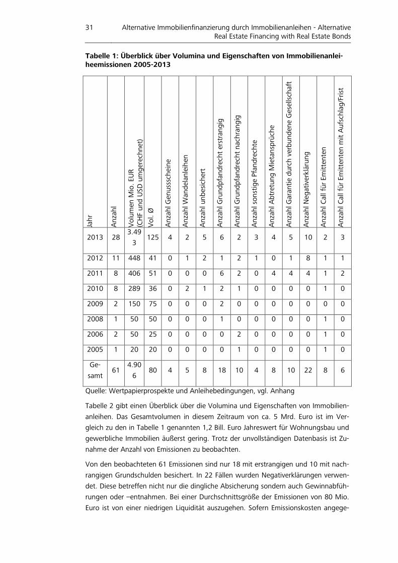
31 Alternative Immobilienfinanzierung durch Immobilienanleihen - Alternative Real Estate Financing with Real Estate Bonds
Tabelle 1: Überblick über Volumina und Eigenschaften von Immobilienanlei-heemissionen 2005-2013
Jah
r
An
zah
l
Vo
lum
en M
io. EU
R
(CH
F und
USD
um
ger
echnet
)
Vo
l. Ø
An
zah
l Gen
usss
chei
ne
An
zah
l Wan
del
anle
ihen
An
zah
l un
bes
ich
ert
An
zah
l Gru
nd
pfa
nd
rech
t er
stra
ng
ig
An
zah
l Gru
nd
pfa
nd
rech
t nac
hra
ng
ig
An
zah
l so
nst
ige
Pfan
dre
chte
An
zah
l Ab
tret
ung
Mie
tan
sprü
che
An
zah
l Gar
anti
e d
urc
h v
erb
un
den
e G
esel
lsch
aft
An
zah
l Neg
ativ
erkl
ärun
g
An
zah
l Cal
l für
Emit
ten
ten
An
zah
l Cal
l für
Emit
ten
ten m
it A
ufs
chla
g/F
rist
2013 28 3.49
3 125 4 2 5 6 2 3 4 5 10 2 3
2012 11 448 41 0 1 2 1 2 1 0 1 8 1 1
2011 8 406 51 0 0 0 6 2 0 4 4 4 1 2
2010 8 289 36 0 2 1 2 1 0 0 0 0 1 0
2009 2 150 75 0 0 0 2 0 0 0 0 0 0 0
2008 1 50 50 0 0 0 1 0 0 0 0 0 1 0
2006 2 50 25 0 0 0 0 2 0 0 0 0 1 0
2005 1 20 20 0 0 0 0 1 0 0 0 0 1 0
Ge-
samt 61
4.90
6 80 4 5 8 18 10 4 8 10 22 8 6
Quelle: Wertpapierprospekte und Anleihebedingungen, vgl. Anhang
Tabelle 2 gibt einen Überblick über die Volumina und Eigenschaften von Immobilien-
anleihen. Das Gesamtvolumen in diesem Zeitraum von ca. 5 Mrd. Euro ist im Ver-
gleich zu den in Tabelle 1 genannten 1,2 Bill. Euro Jahreswert für Wohnungsbau und
gewerbliche Immobilien äußerst gering. Trotz der unvollständigen Datenbasis ist Zu-
nahme der Anzahl von Emissionen zu beobachten.
Von den beobachteten 61 Emissionen sind nur 18 mit erstrangigen und 10 mit nach-
rangigen Grundschulden besichert. In 22 Fällen wurden Negativerklärungen verwen-
det. Diese betreffen nicht nur die dingliche Absicherung sondern auch Gewinnabfüh-
rungen oder –entnahmen. Bei einer Durchschnittsgröße der Emissionen von 80 Mio.
Euro ist von einer niedrigen Liquidität auszugehen. Sofern Emissionskosten angege-
32 Alternative Immobilienfinanzierung durch Immobilienanleihen - Alternative Real Estate Financing with Real Estate Bonds
ben waren, lagen diese zwischen 0,4 bis 6,35 Prozent, wobei teilweise auch Ausga-
beaufschläge von bis zu 5 Prozent erhoben wurden.
Neun der Anleihen sind Wandelschuldverschreibungen oder Genussscheine. Diese
sind grundsätzlich als Instrumente zur Eigenkapitalsubstitution anzusehen und wer-
den an dieser Stelle nicht gesondert analysiert.
3.5.2 Unternehmensfinanzierung mit Immobilienanleihen
Neben Anleihen, die der Finanzierung der allgemeinen Geschäftstätigkeit dienen, gibt
es Emissionen, bei denen der Verwendungszweck des Emissionserlöses zwar grob de-
finiert, aber nicht konkret spezifiziert ist. Dies impliziert eine hohe Informationsasym-
metrie zwischen Emittent und Anleger.60
Sind die Anleihen nicht mit einer werthalti-
gen Grundschuld ausgestattet, sollten die Kupons aufgrund der Unsicherheit entspre-
chend hoch sein. Am Markt sind bei derartigen Anleihen aber auch Kupons von 5
Prozent und darunter zu beobachten. Dies impliziert, dass das Risiko von den Anle-
gern nicht adäquat bewertet wird und von den Emittenten genutzt wird, um niedrige
Risikoprämien zu erreichen.
Aufgrund der o.a. Unsicherheit ist bei einer Vielzahl der Emissionen von einem Credit
Spread auszugehen, welcher durch den Default Spread dominiert sein sollte. Die Ra-
tings und die seltenen Callrechte lassen einen niedrigen Callability Spread erwarten.
Die Heterogenität der Emittenten und der rechtlichen Ausgestaltung der Emissionen
führt zu unterschiedlichen Liquidity Spreads und Missing Reputation Spreads.
Da selten erstrangige Grundpfandrechte zur Besicherung verwendet werden, ist da-
von auszugehen, dass Senior Tranchen anderweitig zu besseren Konditionen finan-
ziert werden und Immobilienanleihen eher im Bereich der Junior Tranche oder Mez-
zanine Anwendung finden. Teilweise bleibt auch das gesamte Grundbuch durch Ne-
gativerklärung unbelastet. Die Anleiheemissionen stehen dann im gleichen Rang mit
anderen Verbindlichkeiten, haben allerdings auch nicht notwendigerweise einen Be-
zug zum Beleihungs- oder Verkehrswert des Grundstücks. Wenn Emittenten nur die
Stammeinlage oder sogar ein negatives Eigenkapital ausweisen, tragen Immobilien-
anleihen auch anteilig hohe Risiken. Insbesondere wenn über die Bestandhaltung hi-
naus Repositionierung und Handelsgewinne den Fokus der (dann riskanten) Ge-
schäftstätigkeit darstellen, muss die Höhe der Credit Spreads kritisch betrachtet wer-
den.
3.5.3 Fallbeispiel Bestandfinanzierung
Die Deutsche Annington SE, eines der großen bestandhaltenden Wohnungsunter-
nehmen, hat die beobachteten großvolumigen Emissionen der Deutschen Annington
B.V. im Rahmen ihres Debt Issuance Program als Anschlussfinanzierung für auslau-
60 Die Informationsasymmetrie kann bspw. durch Ratings gemindert werden. Loritz (2010) S.1 f. sieht Ratings in intransparenten Immobilienmärkten kritisch.
33 Alternative Immobilienfinanzierung durch Immobilienanleihen - Alternative Real Estate Financing with Real Estate Bonds
fende CMBS genutzt. Die Anleihen sind nicht grundpfandrechtlich besichert. Die
Deutsche Annington SE tritt als Garantin auf. Emittentin und Garantin verpflichten
sich in einer Negativerklärung keine Eintragung dinglicher Sicherungsrechte einzutra-
gen oder fortbestehen zu lassen, wobei hiervon Sicherungsrechte für verbriefte Kapi-
talmarktverbindlichkeiten ausgenommen sind.61
Allerdings ist die Garantin bezüglich
des Eingehens von Finanzverbindlichkeiten eingeschränkt.62
Die Anleihen erhalten
kein eigenes Rating, stattdessen wird auf das Unternehmensrating abgestellt.63
Im
Detail bestehen Unterschiede zwischen den einzelnen Emissionen. Die Final Terms der
A1HRVD geben der Emittentin beispielweise das Recht der vorzeitigen Rückzahlung
zu einem Wahlrückzahlbetrag, der sich aus dem Nennwert und den abgezinsten aus-
stehenden Zinszahlungen errechnet. Der Zinssatz für die Abzinsung ergibt sich aus
der Benchmarkrendite zuzüglich 35 Basispunkte. Die Benchmarkrendite ist als Rendite
einer Anleihe der Bundesrepublik Deutschland mit einer Laufzeit, die der Restlaufzeit
der Anleihe definiert.64
Für die Emissionskosten ist ein Betrag in Höhe von 3,005 Mio. Euro bei einem Emissi-
onsvolumen von 500 Mio. Euro angegeben, was 0,6 Prozent entspricht. Bei den beo-
bachteten Emissionen ist aufgrund der hohen Volumina ein geringer Liquidity Spread
zu erwarten. Der Default Spread dieser Anleihen sollte denen von Unternehmensan-
leihen mit gleichem Rating entsprechen. Zudem ergeben sich keine Anhaltspunkte,
die auf einen hohen Spread bezüglich mangelnder Reputation schließen lassen. Mit
zunehmender Laufzeit ist ein steigender Kupon zu beobachten, was einer normalen
Zinsstrukturkurve entspricht. Die spezifischen Callrechte der A1HRVD sollten aufgrund
des Marktwertbezugs nur zu einem geringen Callability Spread führen. Eine Erwirt-
schaftung der Kupons in der genannten Höhe durch Bestandhaltung erscheint realis-
tisch.
3.5.4 Fallbeispiel Projektentwicklung
Projektentwicklungen zeichnen sich i.d.R durch eine hohe Eigenkapitalrendite bei
entsprechendem Risiko aus. Ein positiver Cashflow, welcher für Zins und (endfällige)
Tilgung verwendet werden kann, wird häufig erst bei Projektabschluss erwirtschaftet,
sodass laufende Zinszahlungen auch aus Eigen- und Fremdkapital finanziert werden
müssen. Für den Projekterfolg ist die Liquidität des Kapitalnehmers bis zur Abschluss
von höchster Priorität. Die Bemessung der Laufzeit ist in diesem Zusammenhang von
besonderer Bedeutung. Bei Verzögerungen kann eine Finanzierungsverlängerung er-
forderlich sein, die dann mit den Anleihegläubigern abzustimmen ist. Praktikabler ist
61 Vgl. Deutsche Annington B.V. (2013a), S. 96 f. 62 Vgl. Deutsche Annington B.V. (2013b), S. 29 f., § 11 Verpflichtungserklärungen regelt die Bedingungen zur Einschränkung des Eingehens von Finanzmarktverbindlichkeiten, Einhalten des konsolidierten Deckungsgrads und Gesamtbetrag des unbelasteten Vermögens und das Berichtswesen. 63 Vgl. Deutsche Annington B.V. (2013b), S. 59. 64 Vgl. Deutsche Annington B.V. (2013b), S. 14 f.
34 Alternative Immobilienfinanzierung durch Immobilienanleihen - Alternative Real Estate Financing with Real Estate Bonds
eine über die geplante Projektdauer hinausgehende Laufzeit mit einem vorzeitigen
Tilgungsrecht. Bei einer normalen Zinsstrukturkurve führt dies zu einem höheren Ba-
siszins und zu einem Spread für die Callability. Zudem ist das Risiko im Vergleich zu
einem Bestandsobjekt größer, was in einem größeren Credit Spread der Anleihe re-
sultiert.
Immobilienanleihen zur Finanzierung von Projektentwicklung sind nur in geringer
Zahl zu beobachten. Nach Schützle (2011) könnte ein Grund darin liegen, dass Pro-
jektentwickler nur unzureichende Kenntnisse über alternative Finanzierungs-
instrumente haben.65
Zudem kann bei einer Vielzahl von Gläubigern mit heterogener
Kompetenz die professionelle und termingerechte Umsetzung einer eventuell not-
wendigen Prolongation erschwert sein.
Ein Beispiel für eine typische Finanzierung einer Projektentwicklung mittels Immobi-
lienanleihen ist die die Emission der Cloud No7 GmbH mit einem Volumen von 35
Mio. Euro. Diese weist einen Kupon von 6 Prozent bei einer Laufzeit von 4 Jahren aus
und ist über erstrangige Grundpfandrechte in Höhe von 40 Mio. Euro und die Abtre-
tung der Pachtansprüche aus dem Hotelbetrieb abgesichert.66
Zudem verbleibt ein
Betrag in Höhe von zweimal 6 Prozent aus der Emission zur Absicherung der Zinszah-
lung bei einem Treuhänder, was 50 Prozent des geplanten Zinsaufwands darstellt.67
Das Rating liegt mit BBB im Lower Medium Grade des Investmentgrade. Die Emitten-
tin hat Tilgungsrechte zum Nennbetrag zum 03.01.2016, 03.07.2016 und
03.01.2017.68
Die Kosten der Errichtung werden mit ungefähr 80 Mio. Euro angegeben,69
wobei
nicht ersichtlich ist, ob Finanzierungskosten enthalten sind. Sind hier die Kostengrup-
pen 100 bis 700 der DIN 276 gemeint, wären auch die Zinsen für Fremdkapital
enthalten. Dem steht ein Verkehrswert des fertiggestellten Projekts in Höhe von etwa
91 Mio. Euro gegenüber.70
Die Verwendung der Emissionserlöse ist spezifiziert.71
Vereinfachend kann man den
80 Mio. Euro für die Errichtungskosten die Emissionserlöse von 35 Mio. Euro gege-
65 Vgl. Schützle (2011), S. 135 f. 66 Vgl Cloud No7 GmbH (2013), S. 66. 67 Vgl Cloud No7 GmbH (2013), S. T5. 68 Vgl Cloud No7 GmbH (2013), S. 65. 69 Vgl Cloud No7 GmbH (2013), S. 42. 70 Vgl Cloud No7 GmbH (2013), S. I5. 71 Vgl Cloud No7 GmbH (2013), S. T4 f. Aus der Emission sollen bis zu 15 Mio. € für die Er-richtung und Entwicklung inkl. der Rückführung der Vorfinanzierung und nicht spezifizierte Beträge für Vertriebs- und Verkaufsprovisionen verwendet werden. Weiterhin sollen bis zu 1,5 Mio. € für die Emissionskosten, 6,3 Mio. € für Bankverbindlichkeiten, 3,75 Mio. € zu Befriedi-gung von Forderungen der Gesellschafter, 4,2 Mio. € für die Absicherung der Zinszahlungen, 1,2 Mio. € für laufende Geschäftskosten und etwa 30.000 € für den Treuhänder verwendet werden. Bis auf einen Restbetrag von weiteren 3 Mio. € ist das Emissionsvolumen somit ver-plant.
35 Alternative Immobilienfinanzierung durch Immobilienanleihen - Alternative Real Estate Financing with Real Estate Bonds
nüberstellen. Die Differenz von 45 Mio. Euro zeigt, dass ohne Mittel aus geplanten
Verkäufen nach Makler- und Bauträgerverordnung (MaBV) oder weitere Aufnahme
von Fremd- oder Eigenmitteln eine Finanzierung des Projekts bis zur Fertigstellung
nicht möglich ist. Somit besteht ein hohes Vertriebsrisiko.72
Aufgrund des Geschäftsmodells ist anzunehmen, dass der Default Spread den Credit
Spread dominiert. Rating und Laufzeit sind vergleichbar zu den beobachteten Be-
standsemissionen. Der Callability Spread für die Sondertilgungsrechte kann eine Erklä-
rung für den höheren Kupon liefern. Aufgrund des geringen Emissionsvolumina ist
zudem eine niedrige Liquidität und somit ein hoher Liquiditiy Spread zu erwarten. Es
scheint weiterhin wahrscheinlich, dass der Anteil des Remaining Gap hoch und auf
den Mangel von Reputation und Track-Record zurückzuführen ist. Im Vergleich zu
marktüblichen Bankkonditionen ist der Kupons eher niedrig. Eine Erwirtschaftung der
Kuponzahlungen durch die Projektentwicklung erscheint entsprechend realisierbar.
3.5.5 Fallbeispiel Immobilienanleihe im Insolvenzfall
Als prominenter Nachweis für Diskrepanzen zwischen suggerierter und tatsächlicher
Sicherheit kann die WGF AG dienen, die im Dezember 2012 Insolvenz anmeldete. Die
WGF AG stellte als Sicherungsinstrumente erstrangige Grundschulden, Covenants,
Mittelverwendungs- und Treuhandverträge. Jedoch wies die WGF AG zum
31.12.2009 laut Prospekt der Anleihe WGFH07 vom 17.09.2010 ein Eigenkapital in
Höhe von ca. 7 Mio. Euro bei einem Stammkapital von 3 Mio. Euro im Verhältnis zu
Verbindlichkeiten in einer Höhe von ca. 150 Mio. Euro, hiervon ca. 141 Mio. Euro als
Anleihekapital, aus.73
Dies entspricht einem Verhältnis von Stammeinlage zu Anleihe-
verbindlichkeit in Höhe von 3 zu 141 oder einem Anteil von 2,1 Prozent.74
Diese Informationen waren bei genauer Lektüre der Prospekte zugänglich. Es er-
scheint jedoch fraglich, ob dies der Mehrheit der Anleger bewusst war, als sie die An-
leihen zeichneten. Selbst für fachkundige Anleger war nicht erkennbar, dass die Ge-
sellschaft in 2009 bereits ein negatives Eigenkapital von ca. 7 Mio. Euro aufwies. Der
Jahresabschluss wurde rückwirkend geändert.75
Im Insolvenzplan werden für die Hy-
pothekenanleihegläubiger in Phase 1 der Rückzahlung (2013 bis 2015) Beträge von
50,7 Mio. Euro und in Phase 2 (2014 bis 60 Prozent der Forderung erfüllt sind) 53,4
Mio. Euro in Aussicht gestellt.76
Bemerkenswert ist, dass im Insolvenzplan dahinge-
hend argumentiert wird, dass im Fall einer Verwertung auf dem Wege der Zwangs-
versteigerung, für den angebundenen Projektentwicklungsbestand kein Verwer-
72 Vgl. hierzu auch Cloud No7 GmbH (2013), S. 12 zu Finanzierungsrisiken. 73 Vgl. WGF AG (2010), S. 118. 74 Am 21.02.2014 notierte die Anleihe mit 13,00, vgl. Kursdaten der Börse Düsseldorf AG. 75 Vgl. WGF AG (2012). 76 Vgl. WGF AG (2013), S. 18.
36 Alternative Immobilienfinanzierung durch Immobilienanleihen - Alternative Real Estate Financing with Real Estate Bonds
tungserlös realisierbar wäre.77
Folgt man dieser Argumentation lässt sich die Sinnhaf-
tigkeit von erstrangigen Grundpfandrechten und aufwendigen Treuhand- und Mittel-
verwendungsverträgen zumindest anzweifeln. Bei laufenden Projektentwicklungen
erfolgt zwar i.d.R. keine lineare Wertsteigerung, abgeschlossene Genehmigungs- und
Verpachtungsprozesse leisten diese aber zumindest etappenweise, da somit maßgeb-
liche Risiken entfallen.
Zwischenzeitlich wurde Klage auf Schadenersatz wegen Prospekthaftung gegen die
Verantwortlichen eingereicht.78
3.6 Fazit
Basel III und Solvency II induzieren eine höhere Attraktivität der Alternativen zur
bankbasierten Immobilienfinanzierung. Weiterhin ist in Anbetracht des aktuellen
Niedrigzinsumfelds und des zunehmenden Margendrucks aus Sicht der Anleger die
höhere Rendite ein wesentliches Argument für die Vorteilhaftigkeit von Immobilien-
anleihen. Anleihen können für die Immobilienfinanzierung eine potentielle Alternative
darstellen. Welche Bedeutung sie aktuell und in Zukunft haben werden, muss nicht
zuletzt aufgrund der unzureichenden Datenbasis offen bleiben. Vieles spricht dafür,
dass es sich auch weiterhin um ein Nischenprodukt handeln wird.
Maßgebliches Kriterium für den Erfolg ist die Frage, ob die Finanzierungskosten bei
Modellen mit Anleihen einem Wirtschaftlichkeitsvergleich mit anderen Alternativen
standhalten. Aus der Sicht der Emittenten von Immobilienanleihen besteht die Vor-
teilhaftigkeit von Immobiliendarlehen darin, durch die Elimination eines Intermediärs
zu günstigeren Finanzierungskosten zu kommen.79
In der Vergangenheit wurden
auch Anleihen zu sehr günstigen Konditionen ausgegeben, obwohl die emittierenden
Unternehmen keine ausreichende Bonität für ein Bankdarlehen ausweisen konnten.
Unter dem Aspekt des Anlegerschutzes ist dies bedenklich.80
77 Vgl. WGF AG (2013), S.21. 78 Vgl. Leykam (2014). 79 Für Mittelstandanleihen ohne Immobilienbezug vgl. Horsch/Sturm (2007). 80 Vgl. Katzung (2013).
37 Real estate development – Risk and Solvency
4 Real estate development – Risk and Solvency
Abstract
Making the initial decision for a real estate development project is hard. Transaction
costs for the site acquisition are high and the outcome of the project is uncertain.
Regarding zero recourse project finance, only a finished project can ensure a smooth
payback of the invested capital. Therefore the solvency of the developer until comple-
tion is of utmost importance. Risks in the development process should be reflected in
the financing structure. In the end, the careful consideration of the expected out-
comes should result in a reasonable bid price for the site and a finance structure that
has a proper risk and return profile for all parties involved. This paper presents a prac-
tical spreadsheet and simulation-based method for decision making in real estate de-
velopment with zero recourse project finance. Simulation-based residual valuation re-
sults are combined with an iteration-based quantification of risk, solvency and return
that helps defining a bid price for the site and possible financing structure. Especially
for unique design developments and alternative financed developments this is of high
value. Although the quality of results is depending on the quality of input data, this
paper can help professionals in real estate development to improve their tools for de-
cision making.
Keywords – Monte Carlo simulation, Risk management, Bid price, Finance structure,
Solvency
4.1 Introduction
This paper presents an extension of common simulation-based approaches of calcu-
lating projects in the real estate development industry. Simulation-based residual
valuation results are combined with an iteration-based quantification of risk, solvency
and return. Finance conditions, in particular the components of the credit spread, are
based on the risk derived from simulation results and further assumptions and not
taken into account by choosing a distribution. The considered components of the
calculated credit spread are the default-, liquidity- and callability spread. In order to
obtain the necessary linkage of the project and the financing the approach is re-
stricted to only consider a trader-developer81 with a zero recourse project finance
structure because the financing of a real estate development in a big real estate
company with a multitude of business branches and sources of cash-flow is not com-
parable concerning requirements of debt and equity providing solvency to ensure the
completion and the future value of the development. It is shown that a simulation-
based approach of calculating projects helps improving decision making concerning
the initial decision for or against a project and is also key for structuring the financing
of the development. A major result lies in a reasonable price for the site and after a
81 The employer of a service developer might want to use a similar approach.
38 Real estate development – Risk and Solvency
positive decision on the structure of the financing ensuring a completion of the pro-
ject and the solvency of the developer.
4.2 Literature review
The development of real estate is a risky venture and the financing is a crucial part of
the development process. The usage of simulation for quantification of values and
risks in real estate development and the financing of real estate development projects
are addressed by several academic publications.
MacFarlane (1995) highlighted the problem of developers underestimating their risks
and therefore seeking too low return. In long-term perspective a disaster for the de-
veloper is inevitable and even worse if the investment is highly geared or if the inves-
tor has a portfolio of similar projects. MacFarlane identifies another major problem
when profits of an earlier development are carried in a later development without
protection against the different possible outcomes. In his opinion these characteris-
tics are common in development companies going bankrupt on the down-side of a
property cycle.
Atherton et al. (2008) find that underestimation of risk pertaining to the project leads
to overestimation concerning the value and consequently the highest possible bid for
the site82. They point out that using a prescriptive model helps identifying the key
variables for the decision making process. Often the rent and the years purchase (yp)
or its counterpart the all-risk-yield (ary), are the most important variables because
they determine the value in the moment of the completion or the end of the void
time83. Yet these are the both variables the developer has the least influence on. Al-
though they expect the final decision being made relative to current assumptions,
they expect the decision maker to be able to make a better decision by assessing the
possible ups and downs and therefore having a better understanding of the risk.
Wiedenmann (2005) presented a system for an optimized decision making in choos-
ing between different development projects. This was done by an equal treatment of
risk and return, which he was not expecting being used in the former return-driven
development industry. His system is designed in a transparent, easy understandable
and user-friendly way. One major result is the identification of 51 parameters re-
garded in an economic calculation. 27 of these parameters are identified as risk bear-
ing and should therefore not be considered via single point parameters but with a
distribution. The remaining 24 are known. Validating the common procedures of
quantifying risk he found the Monte Carlo Simulation superior to other methods, es-
pecially regarding transparency for risk and overall feasibility. The result of his system
is a return figure based on a value-at-risk for each considered project. These results
are made comparable by drawing them into a coordinate system. For easy assess-
82 What should lead on the short run to the fact that the sites are sold to the worst devel-oper. 83 When it is planned to sell the project.
39 Real estate development – Risk and Solvency
ment of these results he also presented a rating system based on a boundary func-
tion that can be implemented in the coordinate system to classify the different pro-
jects. As others before he identifies the major flaw or limitation in this approach in
the input variables.
Gimplewich (2011) presented the ‘Simulation-based excess return model for real es-
tate development’, a methodology for combining Monte Carlo simulation-based risk
assessment with the widely practiced discounted-cash-flow-modelling. It provides an
easy metric for risk and return analysis that helps for decision making.
In spite of those publications empirical studies show that few companies use simula-
tion-based models for decision making in the development process. Bohn et al.
(2002) published a study about risk analysis methods in the German real estate de-
velopment sector. 81 of the approached 300 developers participated and only
12.50 % of them use simulation with probabilistic distributions. The dominant
method was scenario analysis with 80 %. Gehner et al. (2006) conducted a survey to
gain insight in the real estate development process, the risks involved and the risk
analysis and control methods used. They approached 31 companies in the Nether-
lands resulting in 15 participating companies. They achieved similar results as Bohn et
al. (2006) having 80 % positive responds for scenario/sensitivity analysis and 0 % for
probabilistic technique, although intuition/experience and qualitative description
were the dominant techniques (100 %).
Wiegelmann (2012) presented a study on the practice of risk management by real es-
tate developers based on empirical research over seven European countries as of
2004/584. The sample includes 159 organisations of which 69 responded. He sees
evidence that “[...] developers tend to take a more reactive rather than proactive
stance to managing risk [...]” and he sees indications that “[...] the development in-
dustry lacks a formal and structured approach throughout the risk management
process.” (Wiegelmann, 2012 p. 184).
Simulation processes, e.g. Monte Carlo simulation, (10.1 %) and value at risk or
other models based on probability distributions (7.2 %) can be seen as rather un-
common methods used for the assessment of identified risk. (Wiegelmann, 2012 p.
142).
For the use of key indicators and threshold values Wiegelmann (2012) shows interest-
ing results when conducting a differentiated analysis. In this special regard the devel-
oper type affects the features of risk management of the company. “Most of the in-
vestor developers tend to have key indicators and threshold values for their risk man-
agement, whereas, most of the trader developers do not make use from key indica-
tors and threshold values”. In addition to that a differentiated analysis confirms “[...]
the expectation that, as the complexity of projects increases, more sophisticated
84 Netherlands, Germany, United-Kingdom, France Spain, Italy and Switzerland.
40 Real estate development – Risk and Solvency
management and monitoring tools are required to provide effective project and risk
management.” (Wiegelmann, 2012 p. 152)
There might be a potential increase of simulation usage by companies in the after-
math of those studies but in any case it is indicated that improvement in the methods
is of interest. This is especially the case when changes in the financing conditions for
development companies or development projects are expected (Pitschke and Bone-
Winkel 2006, Volquarts and Radner 2011). Developers may try to use alternative
ways of financing their projects. In this regard different major failures or bankruptcies
of real estate companies are notable which were trying to use bonds as a way of fi-
nancing their companies or projects.85
Risk management and finance conditions are also addressed by Walsh (2008). He fo-
cussed on developing a model for risk management for real estate developments by
companies with low equity, allowing them to do project finance in contrast to the
ordinary corporate finance. Analysing the possibilities of zero recourse project finance
(ZRPF) in the time and capital intensive conditions of project developments the object
comes into focus. ‘Zero recourse project finance includes the creation of a special
purpose vehicle for a real estate development project, financed by earmarked funds
without the possibility of recourse and equity of one or more project sponsors’
(Walsh, 2008 p. 38 according to Esty, 2004 p. 25). In short, the advantage of ZRPF
lies in the alignment of interest, reduction of information asymmetry, structuring of
action- and command rights, co-determination and control rights after the conclusion
of a contract as a tool against “hidden action” and “hidden intention”. As disadvan-
tages he lists the higher costs of transaction and the higher demand for coordination
and information. Concerning quantitative method he acknowledges the strengths of
Value-at-Risk (VaR) and Cash-Flow-at-Risk (CFaR) but also sees their single point
measures as their weakness and therefore they do not meet his risk management
target system (Walsh, 2008)
In a critical evaluation of using Monte Carlo simulation as a decision tool in real es-
tate development projects Loizou and French (2012) are stressing the importance of
using the Monte Carlo simulation in a complementary fashion because of the under-
lying flaws of these sorts of calculations. They are rightly arguing that the “Monte
Carlo simulation is still a variation on a mathematical model” and results are therefore
only depending on the input variables (see Loizou and French, 2012 p.207). The qual-
ity of the input data and the chosen distributions are based on available data of the
past or assumptions made by experts. In both ways they have no absolute validation.
They further state that uncertainty resulting from human interaction and decision
making in a development process is most important but toughest to evaluate.
85 (e.g. WGF AG, Deikon GmbH), In particular German ‘Schuldverschreibungen’ with and/or
without a variable component.
41 Real estate development – Risk and Solvency
Gleißner and Wiegelmann (2012) are identifying the capital requirements (based on
VaR) as the overall level of risk. They expect penalisation of development companies
by the capital markets if the companies fail to implement a system of identifying, as-
sessing and managing risks. In opposition to Loizou and French (2012) they are not
as critical concerning the input variables because they do not see an alternative to
the quantification of risk. In short, non-quantified risks are hardly just zero quantified
risks. Looking at the decision making process they see the key benefit of quantitative
methods in dealing with the appropriateness of expected risk/return profiles through
key measures of risk. They also believe in the use of Lower Partial Moments (LPM) as
a way of evaluating interesting parts of probability densities from minus infinite up to
a given threshold.
The synthesis of the reviewed publications assists the idea of this paper to address
the main statements of the reviewed publications in a new model and to close some
shortcomings of existing models. Referring to MacFarlane (1995) it is supposed to
prevent underestimating risk and builds on the recommendations concerning capital
requirements and the usage of VaR and LPM by Gleißner and Wiegelmann (2012). It
addresses the question of Atherton et al. (2008) on the correct bid for the site. The
first step of the theoretical model is comparable to their build-up under the necessary
limitation of ZRPF whose attributes where addressed by Walsh (2008). Concerning
the handling of finance structure, interest rates and the sensitivity in regard of time
and future values it takes a different and more sensitive approach than Atherton et
al. (2008), Gimplewich (2011) and Wiedenmann (2005). This allows especially the
consideration of different finance approaches that could be necessary as predicted by
Pitschke and Bone-Winkel (2006) as well as Volquarts and Radner (2011). The con-
cerns of Loizou and French (2012) about input variables are acknowledged but in ac-
cordance with Gleißner and Wiegelmann (2012) there is no alternative to a quantifi-
cation of risk.
4.3 The model
4.3.1 Fundamentals of residual valuation
A valuation always consists of at least one equation, but generally it is based on mul-
tiple equations. As shown by Atherton et al. (2008) a classic residual valuation ap-
proach is based on one major equation, which can be solved for individual variables
(see Table 1).
The classic approach is based on the following 5 major variables:
Sales price - market value after completion/value after bankruptcy for the unfinished
building (realizable m² and €/m²)
Construction costs (€/m² including all costs of the process but the financing)
Time (construction and void)
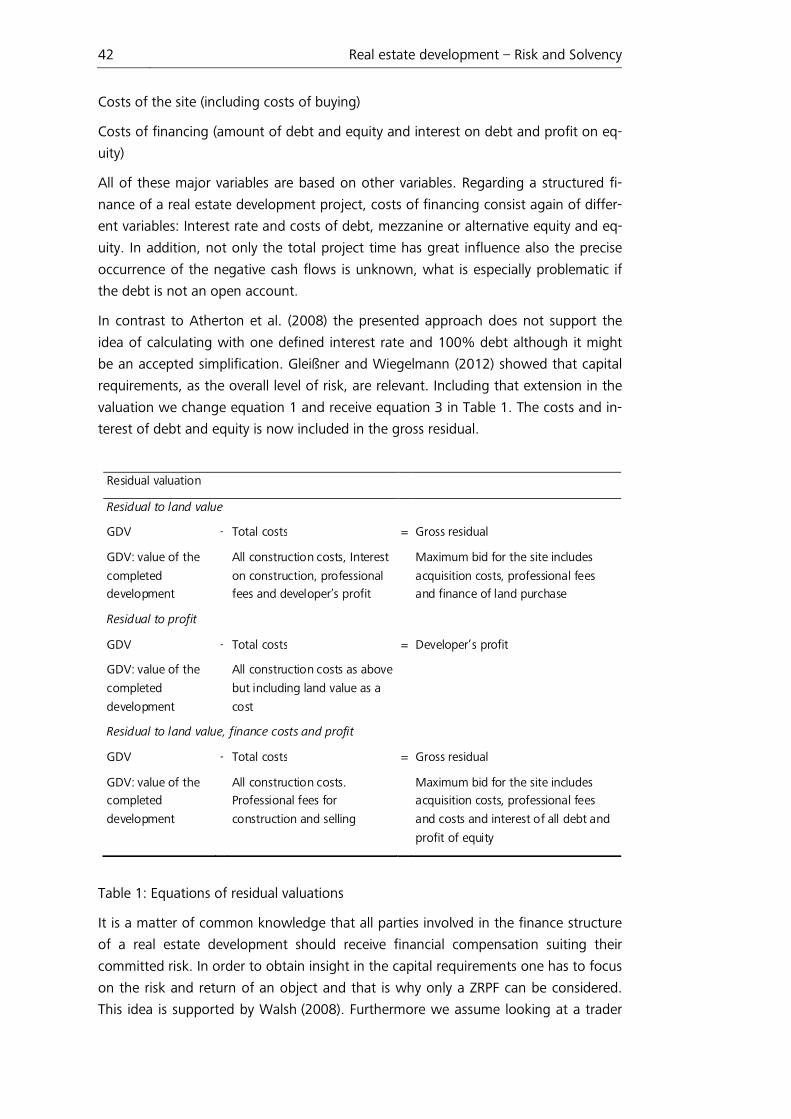
42 Real estate development – Risk and Solvency
Costs of the site (including costs of buying)
Costs of financing (amount of debt and equity and interest on debt and profit on eq-
uity)
All of these major variables are based on other variables. Regarding a structured fi-
nance of a real estate development project, costs of financing consist again of differ-
ent variables: Interest rate and costs of debt, mezzanine or alternative equity and eq-
uity. In addition, not only the total project time has great influence also the precise
occurrence of the negative cash flows is unknown, what is especially problematic if
the debt is not an open account.
In contrast to Atherton et al. (2008) the presented approach does not support the
idea of calculating with one defined interest rate and 100% debt although it might
be an accepted simplification. Gleißner and Wiegelmann (2012) showed that capital
requirements, as the overall level of risk, are relevant. Including that extension in the
valuation we change equation 1 and receive equation 3 in Table 1. The costs and in-
terest of debt and equity is now included in the gross residual.
Table 1: Equations of residual valuations
It is a matter of common knowledge that all parties involved in the finance structure
of a real estate development should receive financial compensation suiting their
committed risk. In order to obtain insight in the capital requirements one has to focus
on the risk and return of an object and that is why only a ZRPF can be considered.
This idea is supported by Walsh (2008). Furthermore we assume looking at a trader
Residual valuation
Residual to land value
GDV - Total costs = Gross residual
GDV: value of the
completed
development
All construction costs, Interest
on construction, professional
fees and developer’s profit
Maximum bid for the site includes
acquisition costs, professional fees
and finance of land purchase
Residual to profit
GDV - Total costs = Developer’s profit
GDV: value of the
completed
development
All construction costs as above
but including land value as a
cost
Residual to land value, finance costs and profit
GDV - Total costs = Gross residual
GDV: value of the
completed
development
All construction costs.
Professional fees for
construction and selling
Maximum bid for the site includes
acquisition costs, professional fees
and costs and interest of all debt and
profit of equity

43 Real estate development – Risk and Solvency
developer to have a defined exit. When we also consider the possibility of insolvency
and therefore the possibility of an unfinished development we have to include the
following possibilities:
Project scenarios
1) Project finished c<(d+e) s<c and d<s Loss of e
2) Project finished c<(d+e) s>c and s<d+e Loss of e
3) Project finished c<(d+e) s>c and s>d+e Gain of e
4) Project unfinished/insolvency c>(d+e) s>d Loss of e
5) Project unfinished insolvency c>(d+e) s<d Loss of d and e
6) Project rejected before start
c Total construction costs (incl. fees, interest and costs of debt and cost for the site incl. fees)
d Debt
e Equity
s Sales price minus cost of selling
Table 2: Project scenarios
Under the presented assumptions it is recognizable that:
• Positive cash-flow can only be generated by selling the object.86 • An unfinished project might not be able to secure the debt at all times. • In contrast to common finance, real estate finance is mostly based on mort-
gages as a way of reducing risk for the (main) creditor. Problems with that approach arise when looking at values of unfinished developments and zero recourse project finance. The mortgage results in a priority in the reclama-tion, but values are not necessarily sufficient to fulfil the claim of the creditor.
• The commitment to the project by debt partners is quite irreversible. • The completion of the project is therefore of utmost importance and depends
heavily on an ensured solvency of the project. • To avoid insolvency, all possible cash-flows until completion must be covered
by debt or equity.87 • The possible losses have to be compensated by equity or the risk premium.
Furthermore the following points have to be considered:
• Delay in the process can influence the market value and the predicted cash-flows.
• Delay can influence the construction costs.
86 Note that after a completion and a successful tenancy a trader-developer could also change its business-model and it is could be possible for him to provide the debt-service of a refinancing with the rental-income or it could be a redevelopment when in a planning phase with positive cash flow due to tenancy. 87 or their substitutes.
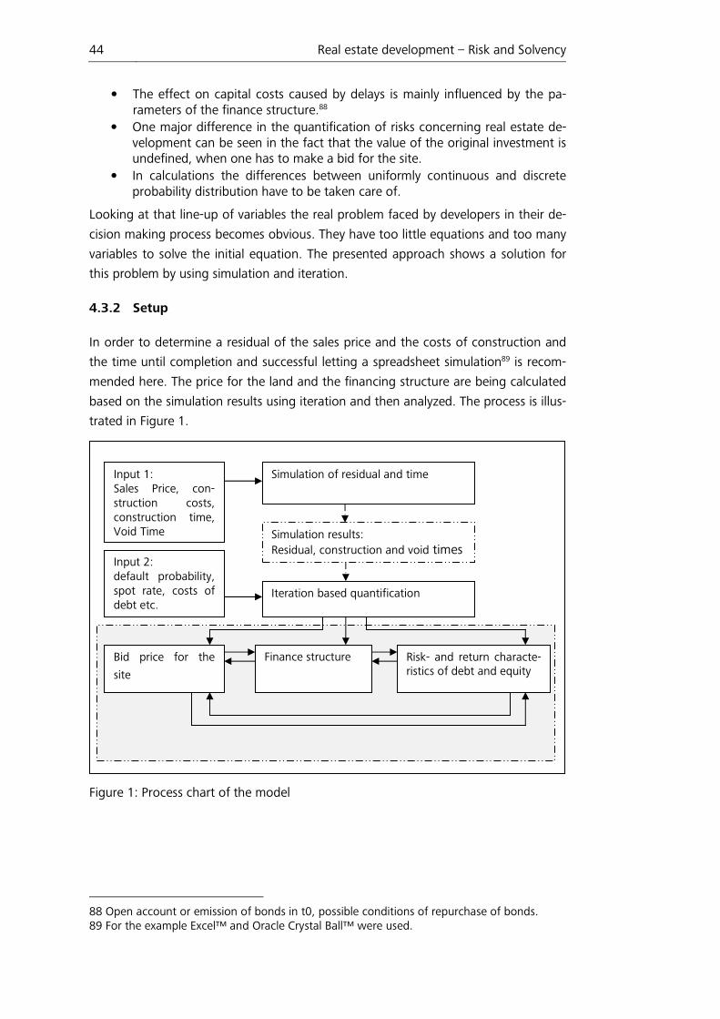
44 Real estate development – Risk and Solvency
• The effect on capital costs caused by delays is mainly influenced by the pa-rameters of the finance structure.88
• One major difference in the quantification of risks concerning real estate de-velopment can be seen in the fact that the value of the original investment is undefined, when one has to make a bid for the site.
• In calculations the differences between uniformly continuous and discrete probability distribution have to be taken care of.
Looking at that line-up of variables the real problem faced by developers in their de-
cision making process becomes obvious. They have too little equations and too many
variables to solve the initial equation. The presented approach shows a solution for
this problem by using simulation and iteration.
4.3.2 Setup
In order to determine a residual of the sales price and the costs of construction and
the time until completion and successful letting a spreadsheet simulation89 is recom-
mended here. The price for the land and the financing structure are being calculated
based on the simulation results using iteration and then analyzed. The process is illus-
trated in Figure 1.
Figure 1: Process chart of the model
88 Open account or emission of bonds in t0, possible conditions of repurchase of bonds. 89 For the example Excel™ and Oracle Crystal Ball™ were used.
Input 1: Sales Price, con-struction costs, construction time, Void Time
Input 2: default probability, spot rate, costs of debt etc.
Simulation of residual and time
Simulation results: Residual, construction and void times
Iteration based quantification
Bid price for the
site
Finance structure Risk- and return characte-ristics of debt and equity
45 Real estate development – Risk and Solvency
4.3.3 Simulation of Residual and Time:
Looking at a trader-developer, the quantification of the value when the construction
is finished or after a certain void time equals the market-value. The precise quantifica-
tion of that market-value is difficult, because it is mainly influenced by the All-Risk-
Yield (ary) and the Years Purchase (yp) which both are also depending of the time of
completion. The expected void and construction times are also hard to predict. Fur-
thermore there are a lot of arguments going on about the appropriate valuation
methods, especially looking at the German Valuation Methods and their Anglo-Saxon
counterparts. For a review see Schnaidt and Sebastian (2011). Holthaus (2007) de-
scribes a model using historic simulation and multiple regressions based on real time
data and not empirical data as advancement in the real estate development industry.
As stated before the risks of property cycles for a developer were already addressed
by MacFarlane (1995). It can be concluded that applying a distribution (density func-
tion) in contrast to single point values is of best practice for the addressed purpose.
This means a simple residual valuation approach with a developer calculation with
sensitivity and scenario analysis is not sufficient especially when regarding unstable
financial and real estate markets or unique feature properties. The parameters pre-
sented by Wiedenmann (2005) are a broad basis. In applied practice a further sup-
plementation and a split up are necessary. This is especially necessary for the differ-
ent parts of the construction costs. The quality of input parameters highly depends
on expertise of the developer or his external service providers. For this example to be
easily presentable an orientation towards the example parameters and input values
of Atherton et al (2008) seems practicable.
After the quantification of the market value we are looking towards the quantifica-
tion of the construction costs (including planning etc. but without interest on capital).
Table 3 shows the input for the residual simulation and the calculation after the simu-
lation and Table 4 the correlations between variables for the simulation. The inputs
shown for finance are not relevant for the simulation of the residual. They are used in
the subsequent iteration. The parts of the effective interest rate p.a. and the costs of
debt are depending on the type of creditor. In the given example a covered corporate
bond of a special purpose vehicle with zero recourse project finance is considered.
Both tables are derived from the inputs used in Atherton et al. (2008) and adjusted to
the further purposes of this paper.90
90 Note that only the residual is simulated.
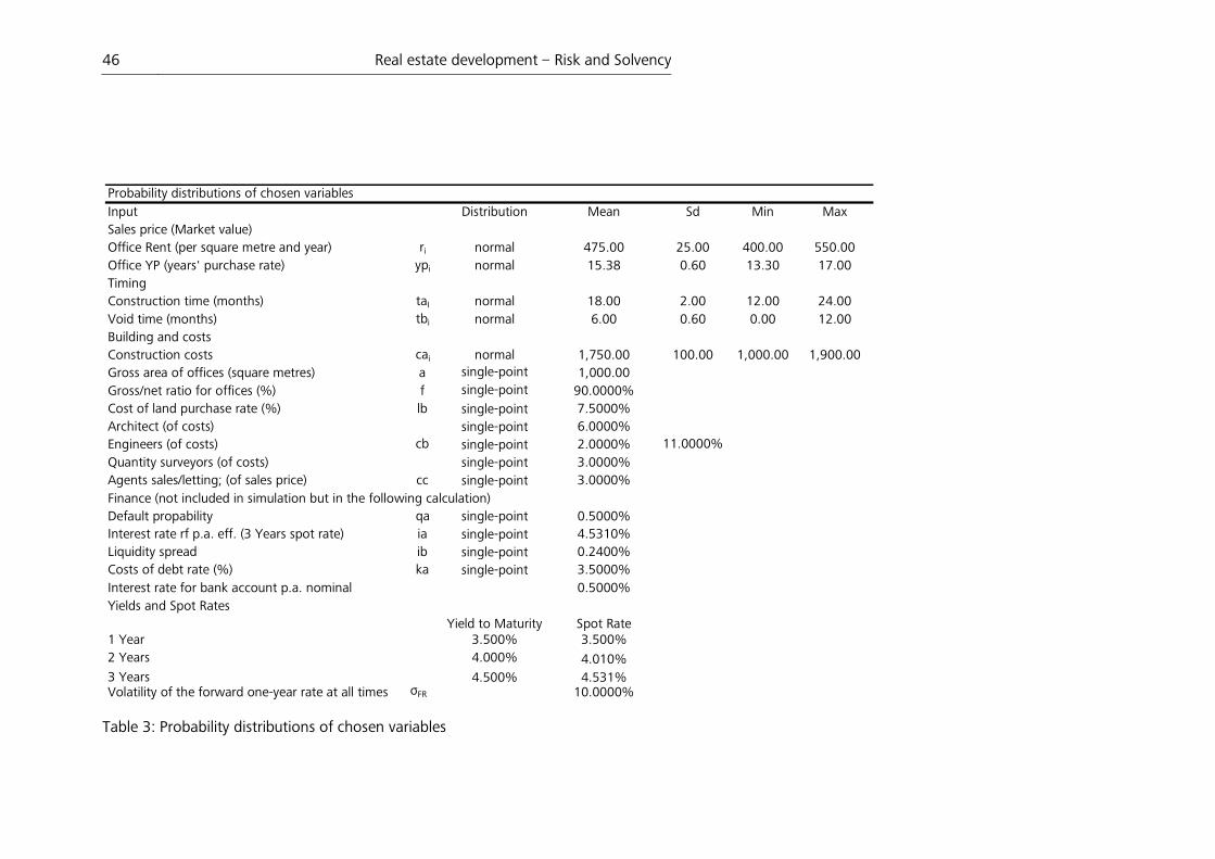
46 Real estate development – Risk and Solvency
Table 3: Probability distributions of chosen variables
Input Distribution Mean Sd Min MaxSales price (Market value)Office Rent (per square metre and year) ri normal 475.00 25.00 400.00 550.00Office YP (years' purchase rate) ypi normal 15.38 0.60 13.30 17.00TimingConstruction time (months) taI normal 18.00 2.00 12.00 24.00Void time (months) tbi normal 6.00 0.60 0.00 12.00Building and costsConstruction costs cai normal 1,750.00 100.00 1,000.00 1,900.00Gross area of offices (square metres) a single-point 1,000.00Gross/net ratio for offices (%) f single-point 90.0000%Cost of land purchase rate (%) lb single-point 7.5000%Architect (of costs) single-point 6.0000%Engineers (of costs) single-point 2.0000%Quantity surveyors (of costs) single-point 3.0000%Agents sales/letting; (of sales price) cc single-point 3.0000%
Finance (not included in simulation but in the following calculation)Default propability qa single-point 0.5000%Interest rate rf p.a. eff. (3 Years spot rate) ia single-point 4.5310%Liquidity spread ib single-point 0.2400%Costs of debt rate (%) ka single-point 3.5000%
Interest rate for bank account p.a. nominal 0.5000%Yields and Spot Rates
Yield to Maturity Spot Rate1 Year 3.500% 3.500%2 Years 4.000% 4.010%3 Years 4.500% 4.531%Volatility of the forward one-year rate at all times σFR 10.0000%
Probability distributions of chosen variables
cb 11.0000%
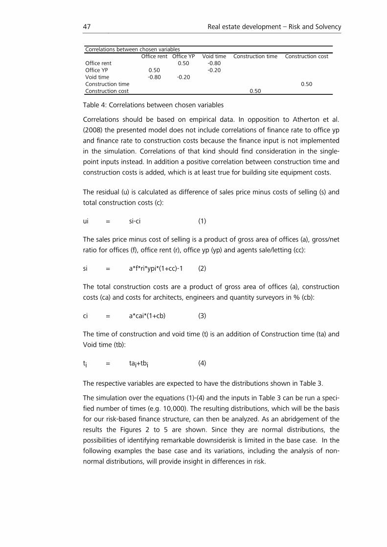
47 Real estate development – Risk and Solvency
Table 4: Correlations between chosen variables
Correlations should be based on empirical data. In opposition to Atherton et al.
(2008) the presented model does not include correlations of finance rate to office yp
and finance rate to construction costs because the finance input is not implemented
in the simulation. Correlations of that kind should find consideration in the single-
point inputs instead. In addition a positive correlation between construction time and
construction costs is added, which is at least true for building site equipment costs.
The residual (u) is calculated as difference of sales price minus costs of selling (s) and
total construction costs (c):
ui = si-ci (1)
The sales price minus cost of selling is a product of gross area of offices (a), gross/net
ratio for offices (f), office rent (r), office yp (yp) and agents sale/letting (cc):
si = a*f*ri*ypi*(1+cc)-1 (2)
The total construction costs are a product of gross area of offices (a), construction
costs (ca) and costs for architects, engineers and quantity surveyors in % (cb):
ci = a*cai*(1+cb) (3)
The time of construction and void time (t) is an addition of Construction time (ta) and
Void time (tb):
ti = tai+tbi (4)
The respective variables are expected to have the distributions shown in Table 3.
The simulation over the equations (1)-(4) and the inputs in Table 3 can be run a speci-
fied number of times (e.g. 10,000). The resulting distributions, which will be the basis
for our risk-based finance structure, can then be analyzed. As an abridgement of the
results the Figures 2 to 5 are shown. Since they are normal distributions, the
possibilities of identifying remarkable downsiderisk is limited in the base case. In the
following examples the base case and its variations, including the analysis of non-
normal distributions, will provide insight in differences in risk.
Correlations between chosen variablesOffice rent Office YP Void time Construction time Construction cost
Office rent 0.50 -0.80Office YP 0.50 -0.20Void time -0.80 -0.20Construction time 0.50Construction cost 0.50
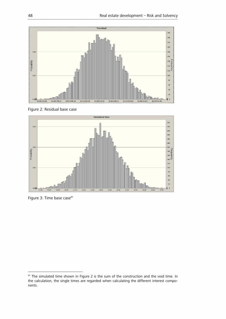
48
Figure 2: Residual base case
Figure 3: Time base case91
91 The simulated time shown in Fithe calculation, the single times anents.
Real estate development – Risk and S
Figure 2 is the sum of the construction and the void are regarded when calculating the different interest
Solvency
id time. In st compo-
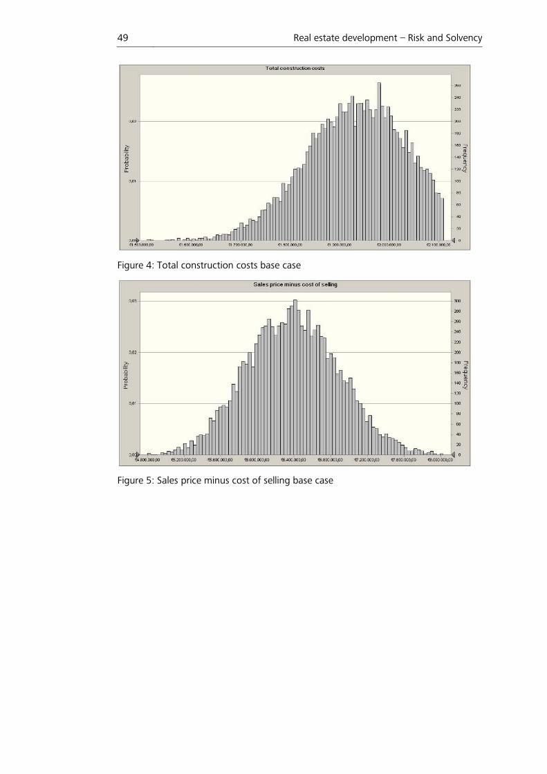
49
Figure 4: Total cons
Figure 5: Sales price
Real estate development
nstruction costs base case
ice minus cost of selling base case
nt – Risk and Solvency

50 Real estate development – Risk and Solvency
4.3.4 Iteration based quantification
The simulation of the residual is followed by calculations for the financing structure.
Iteration solves logically combined equations92 and gives results for previously un-
known multiple variables. A special problem with iteration is oscillation. When having
a residual with discrete distribution and big jumps in the single points, oscillation in
the iteration process can occur. A limitation of trials helps preventing endless itera-
tion. Either the results are satisfying when the iteration stops or one should try to un-
derstand where the oscillation is coming from and then adjust the input or the
boundaries. In this part the used equations and variables are explained. Variables that
are based on the distributions are shown in Table 3.
As mentioned above, the interest rate does not find consideration through a simple
distribution so one has to set up the base and the corresponding components of the
credit spread by equations.
All the parts of the credit spread and the risk free rate p.a. add up to the effective in-
terest rate p.a. for debt. It is an addition of interest rate rf p.a. eff. (ia), liquidity
spread p.a. (ib), callability spread p.a. (ic) and default spread (id) p.a. eff.:
ie = ia+ib+ic+id (5)
The interest rate rf p.a. eff. is based on the maximum time (T). It can be derived of a
risk-free federal bond with the same term with the given spot rates.
A liquidity spread of 24 bps p.a. based on the results of Houweling et al. (2003) is as-
sumed. Bonds for real estate development are most likely of medium volume and
therefore naturally illiquid.
The callability spread p.a. is calculated as the spread of call rights of the issuer by im-
plementing the model of Kalotay et al (1993). For the presented example the follow-
ing adjustments are made: The issuer has the right to call at the end of year 2 that
equals 24 months. By that a call is only possible if the project is finished within a time
of 24 months. If the project takes longer, the planned repayment in year 3 will occur.
This of course has influence on the amount of the interest payments.
We can calculate the default spread p.a. eff. based on the assumption that we have a
cumulated default rate qa in T93. Therefore we have an average default rate of qa/T.
The assumption of qa is a based on the designated risk profile of the debt. In a sim-
ple approach the sum of expected and unexpected loss divided by the maximum time
T and the credit exposure (ce) equals the default spread p.a. in %:
id = (el+ul)/(ce*T) (6)
92 Note that the equations are described with the syntax of Excel™. 93 T is our maximum possible sum of time ta and tb.
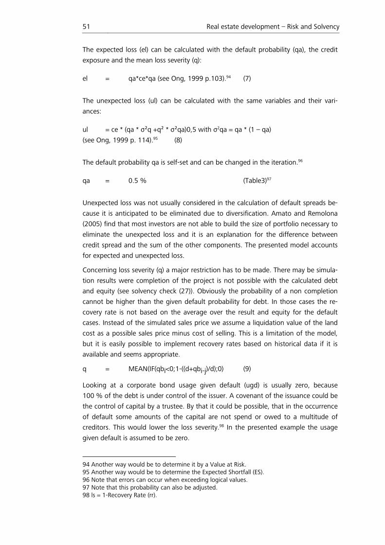
51 Real estate development – Risk and Solvency
The expected loss (el) can be calculated with the default probability (qa), the credit
exposure and the mean loss severity (q):
el = qa*ce*qa (see Ong, 1999 p.103).94 (7)
The unexpected loss (ul) can be calculated with the same variables and their vari-
ances:
ul = ce * (qa * σ²q +q² * σ²qa)0,5 with σ2qa = qa * (1 – qa)
(see Ong, 1999 p. 114).95 (8)
The default probability qa is self-set and can be changed in the iteration.96
qa = 0.5 % (Table3)97
Unexpected loss was not usually considered in the calculation of default spreads be-
cause it is anticipated to be eliminated due to diversification. Amato and Remolona
(2005) find that most investors are not able to build the size of portfolio necessary to
eliminate the unexpected loss and it is an explanation for the difference between
credit spread and the sum of the other components. The presented model accounts
for expected and unexpected loss.
Concerning loss severity (q) a major restriction has to be made. There may be simula-
tion results were completion of the project is not possible with the calculated debt
and equity (see solvency check (27)). Obviously the probability of a non completion
cannot be higher than the given default probability for debt. In those cases the re-
covery rate is not based on the average over the result and equity for the default
cases. Instead of the simulated sales price we assume a liquidation value of the land
cost as a possible sales price minus cost of selling. This is a limitation of the model,
but it is easily possible to implement recovery rates based on historical data if it is
available and seems appropriate.
q = MEAN(IF(qbi<0;1-((d+qbi-j)/d);0) (9)
Looking at a corporate bond usage given default (ugd) is usually zero, because
100 % of the debt is under control of the issuer. A covenant of the issuance could be
the control of capital by a trustee. By that it could be possible, that in the occurrence
of default some amounts of the capital are not spend or owed to a multitude of
creditors. This would lower the loss severity.98 In the presented example the usage
given default is assumed to be zero.
94 Another way would be to determine it by a Value at Risk. 95 Another way would be to determine the Expected Shortfall (ES). 96 Note that errors can occur when exceeding logical values. 97 Note that this probability can also be adjusted. 98 ls = 1-Recovery Rate (rr).
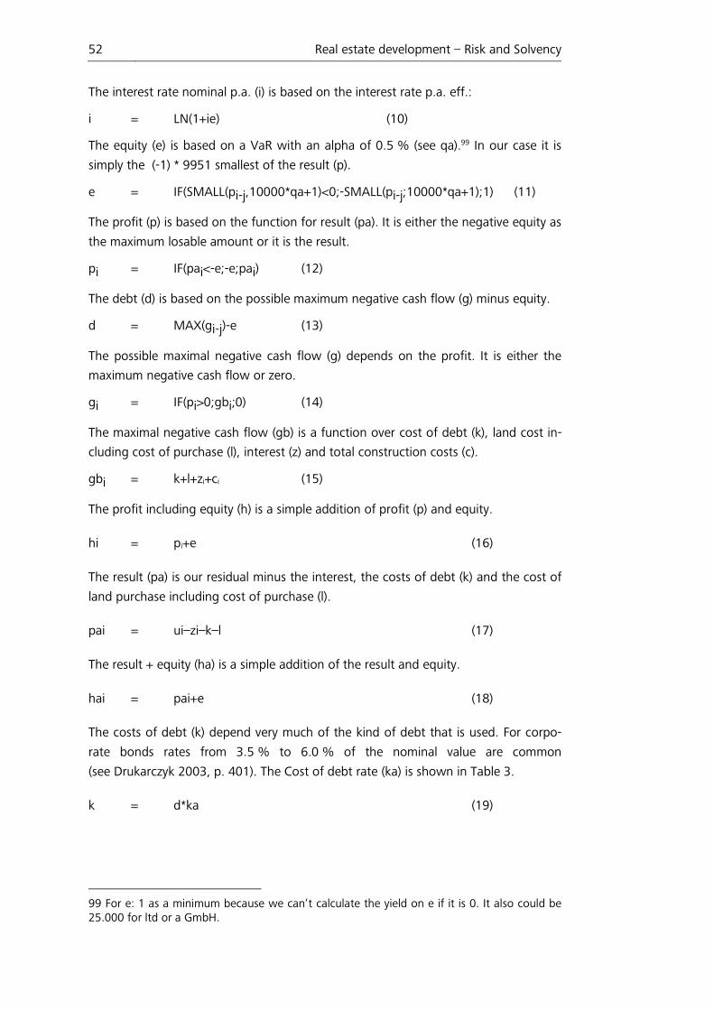
52 Real estate development – Risk and Solvency
The interest rate nominal p.a. (i) is based on the interest rate p.a. eff.:
i = LN(1+ie ) (10)
The equity (e) is based on a VaR with an alpha of 0.5 % (see qa).99 In our case it is
simply the (-1) * 9951 smallest of the result (p).
e = IF(SMALL(pi-j,10000*qa+1)<0;-SMALL(pi-j;10000*qa+1);1) (11)
The profit (p) is based on the function for result (pa). It is either the negative equity as
the maximum losable amount or it is the result.
pi = IF(pai<-e;-e;pai) (12)
The debt (d) is based on the possible maximum negative cash flow (g) minus equity.
d = MAX(gi-j)-e (13)
The possible maximal negative cash flow (g) depends on the profit. It is either the
maximum negative cash flow or zero.
gi = IF(pi>0;gbi;0) (14)
The maximal negative cash flow (gb) is a function over cost of debt (k), land cost in-
cluding cost of purchase (l), interest (z) and total construction costs (c).
gbi = k+l+zi+ci (15)
The profit including equity (h) is a simple addition of profit (p) and equity.
hi = pi+e (16)
The result (pa) is our residual minus the interest, the costs of debt (k) and the cost of
land purchase including cost of purchase (l).
pai = ui–zi–k–l (17)
The result + equity (ha) is a simple addition of the result and equity.
hai = pai+e (18)
The costs of debt (k) depend very much of the kind of debt that is used. For corpo-
rate bonds rates from 3.5 % to 6.0 % of the nominal value are common
(see Drukarczyk 2003, p. 401). The Cost of debt rate (ka) is shown in Table 3.
k = d*ka (19)
99 For e: 1 as a minimum because we can‘t calculate the yield on e if it is 0. It also could be 25.000 for ltd or a GmbH.
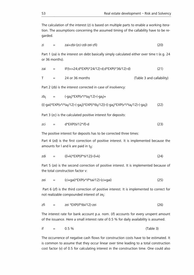
53 Real estate development – Risk and Solvency
The calculation of the interest (z) is based on multiple parts to enable a working itera-
tion. The assumptions concerning the assumed timing of the callability have to be re-
garded.
zi = zai+zbi-(zci-zdi-zei-zfi) (20)
Part 1 (za) is the interest on debt basically simply calculated either over time t (e.g. 24
or 36 months).
zai = IF(t<=24;d*EXP(i*24/12)-d;d*EXP(i*36/12)-d) (21)
T = 24 or 36 months (Table 3 and callability)
Part 2 (zb) is the interest corrected in case of insolvency:
zbi = (-gai)*EXP(v*i*tai/12)-(-gai)+
(((-gai)*EXP(v*i*tai/12)-(-gai))*EXP(i*tbi/12))-((-gai)*EXP(v*i*tai/12)-(-gai)) (22)
Part 3 (zc) is the calculated positive interest for deposits:
zci = d*EXP(ti/12*if)-d (23)
The positive interest for deposits has to be corrected three times:
Part 4 (zd) is the first correction of positive interest. It is implemented because the
amounts for l and k are paid in t0:
zdi = ((l+k)*EXP(if*ti/12))-(l+k) (24)
Part 5 (ze) is the second correction of positive interest. It is implemented because of
the total construction factor v:
zei = (ci+gai)*EXP(v*if*tai/12)-(ci+gai) (25)
Part 6 (zf) is the third correction of positive interest. It is implemented to correct for
not realizable compounded interest of zei:
zfi = zei *EXP(if*tbi/12)-zei (26)
The interest rate for bank account p.a. nom. (if) accounts for every unspent amount
of the issuance. Here a small interest rate of 0.5 % for daily availability is assumed.
if = 0.5 % (Table 3)
The occurrence of negative cash flows for construction costs have to be estimated. It
is common to assume that they occur linear over time leading to a total construction
cost factor (v) of 0.5 for calculating interest in the construction time. One could also
54 Real estate development – Risk and Solvency
assume a factor of 1.0 when the debt amounts to the maximum beginning in t=0 or
a function when variations are planned. In the presented example a linear occurrence
leading to a factor of 0.5 is assumed.
v = 0,5 (Table 3)
To receive an unbiased result, a solvency check has to be implemented due to techni-
cal reasons. Solvency is in most, but not all, cases ensured through the determination
of equity in relation to qa. Basically the maximum negative cash-flow that can occur
in the timeline of the quantification is checked and in case is relevant in the equations
of the credit loss and interest. Insolvency will occur rarely under the assumption of a
qa of 0.5 %. Discrete or skewed distributions can lead to negative impacts resulting
in positive project results where the sales price is higher than all costs, but the total
capital is smaller than the total costs. In that case insolvency would occur before a
sellable project is finished.
gai = IF(0>=(d+e-gbi);d+e-gbi;0) (27)
The credit losses (qb) are a function the possible negative cashflow and the maximal
negative cashflow. It is either the amount of debt minus the value of the land after
selling it in case of insolvency or the result or zero.
qbi = IF(gi=0;IF(gai<0;-d+(la*(1-cc));hai);0) (28)
Equity yield p.a. (y) is derived of profit , equity and time.
yi = IFERROR(EXP((LN(hi/e))/(ti/12))-1;-100%) (29)
The land costs including costs of purchase (l) is either set or estimated and manually
iterated.
l = given or estimated and manually iterated (Table 3/Risk analysis)
The land costs (la) are derived as a quotient of l with the costs of the land purchase
(lb) given by a percentage. This percentage is given in Table 3.
la = l/(1+lb) (30)
lb = 7,5 % (Table 3)
To start the calculation one has to estimate a purchase price including the costs of
the purchase (“l”) for the site100 and EXCEL™ will solve the equations for the given
input using iteration. Precision and iteration attempts have to be set by the user.
100 Note that a maximum purchase price is theoretically set by the maximum residual.
55 Real estate development – Risk and Solvency
4.3.5 Risk analysis and continuation of the iteration
The simulated data and the setup of equations allow focusing on the one variable left
to determine: The cost of the land including the costs of purchase (“l”). There are
now two possibilities:
a) The price of the site is a known offer price and not negotiable or
b) the price is negotiable or unknown and there is a tendering procedure.
For case a) one must evaluate the risk and return and make a decision based on that
analysis.
For case b) one can use the model for optimizing the chosen risk measures by adapt-
ing the price for the site. The highest price reaching the self-set conditions is the
highest offer the developer can make.
One can now manually set “l” to a roughly estimated value and see if the risk meas-
ures accord to the expectations. As said before, the maximum residual value is the
maximum by definition although it is obvious that this value would never match the
expectations for the risk measures. The minimum value below zero is unlikely but
could occur when demands are made by a seller (e.g. public seller). This should lead
to certain cost increase or decrease of the sales price.
As risk or risk adjusted performance measures the Sharpe Ratio, Sortino Ratio,
Omega Ratio, Lower-Partial-Moments, Risk-adjusted and Conditional Value at Risk
are displayed.
Depending on the kind of real estate development object these different risk meas-
ures come into consideration for evaluating yields, profits and capital. A lot of real
estate developments tend to have asymmetric distributions concerning the construc-
tion costs and therefore asymmetric profit distributions. Also when regarding a very
high correlation between construction time and construction costs the downside risk
for equity yield rate rises disproportionally. Therefore downside oriented measures
come into focus. As shown by Kaplan and Knowles (2004) most of these risk meas-
ures are somehow related.
There is no rule for defining an absolute validation of a threshold or value. One has
to use them complementary in regard of the desired targets.
4.4 Case studies
In the following five exemplary cases will be presented in order to give insight in ca-
pabilities of the model.
Assuming a negotiable price an “l” of € 3,100,000 is estimated. Figure 6 shows the
distribution of the profit added to the equity invested for that case. Details of the re-
sults can be seen in Table 5. An adjustment of “l” to a value of 3,500,000 leads to
the distribution for profit and equity shown in Figure 7 and the detailed results in Ta-
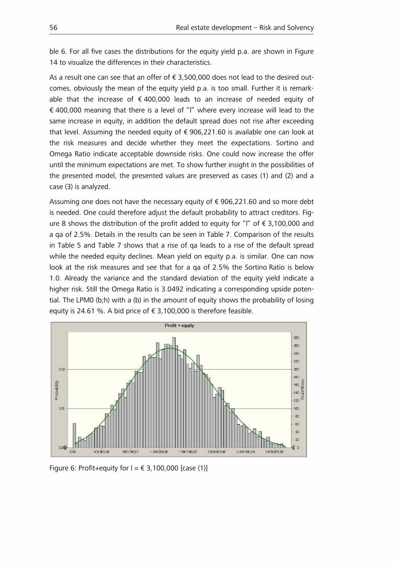
56
ble 6. For all five cases the dist
14 to visualize the differences i
As a result one can see that an
comes, obviously the mean of
able that the increase of € 4
€ 400,000 meaning that there
same increase in equity, in add
that level. Assuming the neede
the risk measures and decide
Omega Ratio indicate acceptab
until the minimum expectations
the presented model, the pres
case (3) is analyzed.
Assuming one does not have th
is needed. One could therefore
ure 8 shows the distribution of
a qa of 2.5%. Details in the res
in Table 5 and Table 7 shows
while the needed equity declin
look at the risk measures and
1.0. Already the variance and
higher risk. Still the Omega Rat
tial. The LPM0 (b;h) with a (b) i
equity is 24.61 %. A bid price o
Figure 6: Profit+equity for l = €
Real estate development – Risk and S
istributions for the equity yield p.a. are shown in
s in their characteristics.
n offer of € 3,500,000 does not lead to the desi
f the equity yield p.a. is too small. Further it is
400,000 leads to an increase of needed eq
re is a level of “l” where every increase will lead
ddition the default spread does not rise after ex
ded equity of € 906,221.60 is available one can
de whether they meet the expectations. Sorti
table downside risks. One could now increase th
ns are met. To show further insight in the possib
esented values are preserved as cases (1) and (2
the necessary equity of € 906,221.60 and so mo
re adjust the default probability to attract credito
of the profit added to equity for “l” of € 3,100,0
results can be seen in Table 7. Comparison of the
s that a rise of qa leads to a rise of the default
lines. Mean yield on equity p.a. is similar. One c
d see that for a qa of 2.5% the Sortino Ratio i
d the standard deviation of the equity yield ind
atio is 3.0492 indicating a corresponding upside
) in the amount of equity shows the probability o
of € 3,100,000 is therefore feasible.
€ 3,100,000 [case (1)]
Solvency
in Figure
sired out-
is remark-
equity of
ad to the
exceeding
n look at
rtino and
the offer
ibilities of
(2) and a
ore debt
itors. Fig-
,000 and
he results
ult spread
can now
is below
indicate a
de poten-
of losing
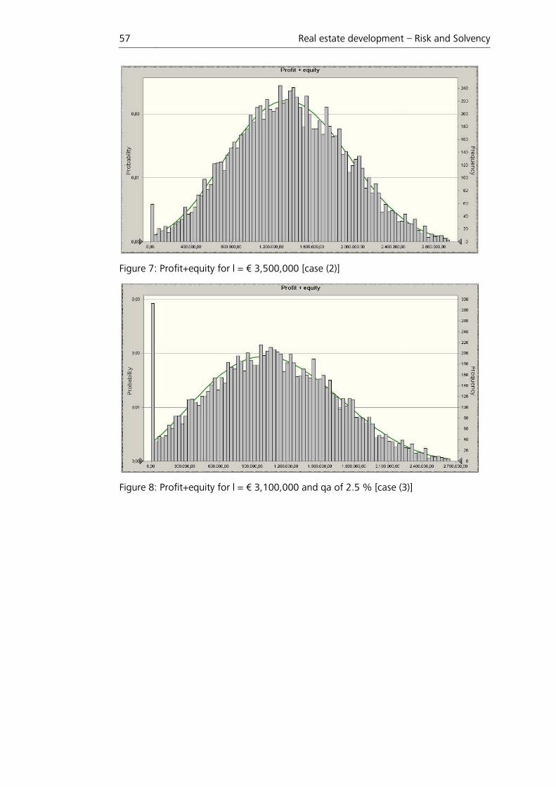
57
Figure 7: Profit+equ
Figure 8: Profit+equ
Real estate development
quity for l = € 3,500,000 [case (2)]
quity for l = € 3,100,000 and qa of 2.5 % [case (3
nt – Risk and Solvency
(3)]
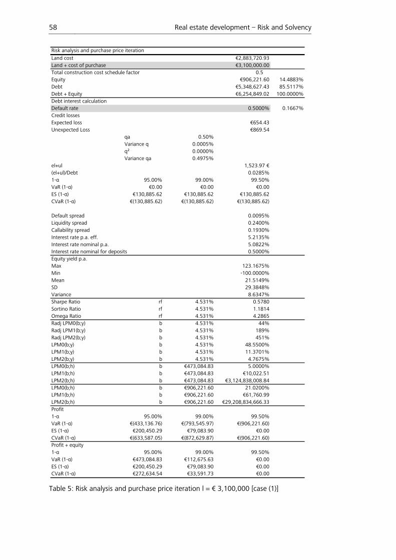
58 Real estate development – Risk and Solvency
Table 5: Risk analysis and purchase price iteration l = € 3,100,000 [case (1)]
Risk analysis and purchase price iteration
Land cost €2,883,720.93Land + cost of purchase €3,100,000.00Total construction cost schedule factor 0.5 Equity €906,221.60 14.4883%Debt €5,348,627.43 85.5117%Debt + Equity €6,254,849.02 100.0000%Debt interest calculationDefault rate 0.5000% 0.1667%Credit lossesExpected loss €654.43Unexpected Loss €869.54
qa 0.50%Variance q 0.0005%q² 0.0000%Variance qa 0.4975%
el+ul 1,523.97 €(el+ul)/Debt 0.0285%1-α 95.00% 99.00% 99.50%VaR (1-α) €0.00 €0.00 €0.00ES (1-α) €130,885.62 €130,885.62 €130,885.62CVaR (1-α) €(130,885.62) €(130,885.62) €(130,885.62)
Default spread 0.0095%Liquidity spread 0.2400%Callability spread 0.1930%Interest rate p.a. eff. 5.2135%Interest rate nominal p.a. 5.0822%
0.5000%Equity yield p.a.Max 123.1675%Min -100.0000%Mean 21.5149%SD 29.3848%Variance 8.6347%Sharpe Ratio rf 4.531% 0.5780Sortino Ratio rf 4.531% 1.1814Omega Ratio rf 4.531% 4.2865Radj LPM0(b;y) b 4.531% 44%Radj LPM1(b;y) b 4.531% 189%Radj LPM2(b;y) b 4.531% 451%LPM0(b;y) b 4.531% 48.5500%LPM1(b;y) b 4.531% 11.3701%LPM2(b;y) b 4.531% 4.7675%LPM0(b;h) b €473,084.83 5.0000%LPM1(b;h) b €473,084.83 €10,022.51LPM2(b;h) b €473,084.83 €3,124,838,008.84LPM0(b;h) b €906,221.60 21.0200%LPM1(b;h) b €906,221.60 €61,760.99LPM2(b;h) b €906,221.60 €29,208,834,666.33Profit1-α 95.00% 99.00% 99.50%VaR (1-α) €(433,136.76) €(793,545.97) €(906,221.60)ES (1-α) €200,450.29 €79,083.90 €0.00CVaR (1-α) €(633,587.05) €(872,629.87) €(906,221.60)Profit + equity1-α 95.00% 99.00% 99.50%VaR (1-α) €473,084.83 €112,675.63 €0.00ES (1-α) €200,450.29 €79,083.90 €0.00CVaR (1-α) €272,634.54 €33,591.73 €0.00
Interest rate nominal for deposits
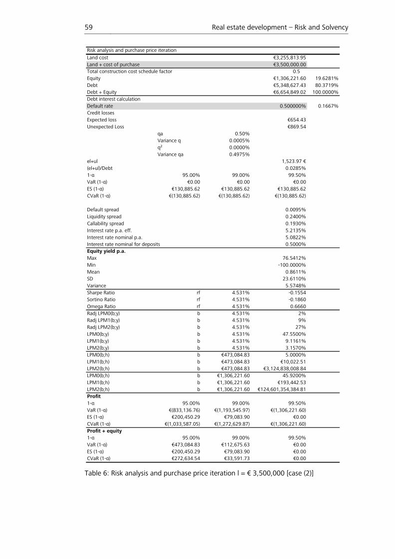
59 Real estate development – Risk and Solvency
Table 6: Risk analysis and purchase price iteration l = € 3,500,000 [case (2)]
Risk analysis and purchase price iteration
Land cost €3,255,813.95Land + cost of purchase €3,500,000.00Total construction cost schedule factor 0.5 Equity €1,306,221.60 19.6281%Debt €5,348,627.43 80.3719%Debt + Equity €6,654,849.02 100.0000%Debt interest calculationDefault rate 0.500000% 0.1667%Credit lossesExpected loss €654.43Unexpected Loss €869.54
qa 0.50%Variance q 0.0005%q² 0.0000%Variance qa 0.4975%
el+ul 1,523.97 €(el+ul)/Debt 0.0285%1-α 95.00% 99.00% 99.50%VaR (1-α) €0.00 €0.00 €0.00ES (1-α) €130,885.62 €130,885.62 €130,885.62CVaR (1-α) €(130,885.62) €(130,885.62) €(130,885.62)
Default spread 0.0095%Liquidity spread 0.2400%Callability spread 0.1930%Interest rate p.a. eff. 5.2135%Interest rate nominal p.a. 5.0822%
0.5000%Equity yield p.a.Max 76.5412%Min -100.0000%Mean 0.8611%SD 23.6110%Variance 5.5748%Sharpe Ratio rf 4.531% -0.1554Sortino Ratio rf 4.531% -0.1860Omega Ratio rf 4.531% 0.6660Radj LPM0(b;y) b 4.531% 2%Radj LPM1(b;y) b 4.531% 9%Radj LPM2(b;y) b 4.531% 27%LPM0(b;y) b 4.531% 47.5500%LPM1(b;y) b 4.531% 9.1161%LPM2(b;y) b 4.531% 3.1570%LPM0(b;h) b €473,084.83 5.0000%LPM1(b;h) b €473,084.83 €10,022.51LPM2(b;h) b €473,084.83 €3,124,838,008.84LPM0(b;h) b €1,306,221.60 45.9200%LPM1(b;h) b €1,306,221.60 €193,442.53LPM2(b;h) b €1,306,221.60 €124,601,354,384.81Profit1-α 95.00% 99.00% 99.50%VaR (1-α) €(833,136.76) €(1,193,545.97) €(1,306,221.60)ES (1-α) €200,450.29 €79,083.90 €0.00CVaR (1-α) €(1,033,587.05) €(1,272,629.87) €(1,306,221.60)Profit + equity1-α 95.00% 99.00% 99.50%VaR (1-α) €473,084.83 €112,675.63 €0.00ES (1-α) €200,450.29 €79,083.90 €0.00CVaR (1-α) €272,634.54 €33,591.73 €0.00
Interest rate nominal for deposits

60 Real estate development – Risk and Solvency
Table 7: Risk analysis and purchase price iteration l = € 3,100,000 and qa of 2.5 %
[case (3)]
Risk analysis and purchase price iteration
Land cost €2,883,720.93Land + cost of purchase €3,100,000.00Total construction cost schedule factor 0.5 Equity €670,107.23 10.5834%Debt €5,661,546.28 89.4166%Debt + Equity €6,331,653.50 100.0000%Debt interest calculationDefault rate 2.500000% 0.8333%Credit lossesExpected loss €4,750.62Unexpected Loss €6,157.55
qa 2.50%Variance qa 0.0047%q² 0.0001%Variance qa 2.4375%
el+ul 10,908.17 €(el+ul)/Debt 0.1927%1-α 95.00% 99.00% 99.50%VaR (1-α) €0.00 €(191,471.20) €(312,926.57)ES (1-α) €190,024.76 €152,713.25 €130,372.79CVaR (1-α) €(190,024.76) €(344,184.45) €(443,299.36)
Default spread 0.0642%Liquidity spread 0.2400%Callability spread 0.2180%
Interest rate p.a. eff. 5.2932%Interest rate nominal p.a. 5.1579%
0.5000%Equity yield p.a.Max 154.6842%Min -100.0000%Mean 22.7360%SD 40.7850%Variance 16.6342%Sharpe Ratio rf 4.531% 0.4464Sortino Ratio rf 4.531% 0.7913Omega Ratio rf 4.531% 3.0492Radj LPM0(b;y) b 4.531% 49%Radj LPM1(b;y) b 4.531% 145%Radj LPM2(b;y) b 4.531% 235%LPM0(b;y) b 4.531% 46.3900%LPM1(b;y) b 4.531% 15.6381%LPM2(b;y) b 4.531% 9.6590%LPM0(b;h) b €161,043.01 5.0000%LPM1(b;h) b €161,043.01 €5,883.62LPM2(b;h) b €161,043.01 €844,023,623.46LPM0(b;h) b €670,107.23 24.6100%LPM1(b;h) b €670,107.23 €74,212.11LPM2(b;h) b €670,107.23 €33,082,561,523.85Profit1-α 95.00% 99.00% 99.50%VaR (1-α) €(509,064.22) €(670,107.23) €(670,107.23)ES (1-α) €117,672.40 €0.00 €0.00CVaR (1-α) €(626,736.62) €(670,107.23) €(670,107.23)Profit + equity1-α 95.00% 99.00% 99.50%VaR (1-α) €161,043.01 €0.00 €0.00ES (1-α) €117,672.40 €0.00 €0.00CVaR (1-α) €43,370.61 €0.00 €0.00
Interest rate nominal for deposits
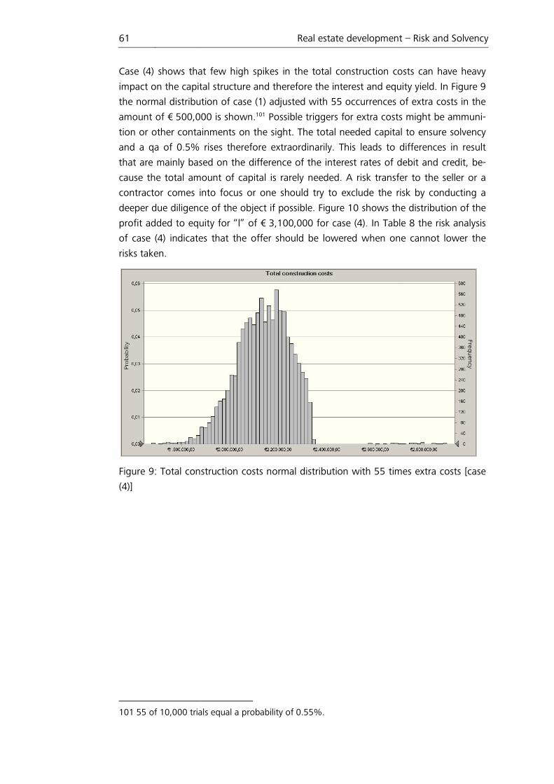
61
Case (4) shows tha
impact on the capit
the normal distribu
amount of € 500,0
tion or other conta
and a qa of 0.5%
that are mainly bas
cause the total am
contractor comes i
deeper due diligenc
profit added to equ
of case (4) indicate
risks taken.
Figure 9: Total con
(4)]
101 55 of 10,000 tria
Real estate development
hat few high spikes in the total construction co
pital structure and therefore the interest and equ
ution of case (1) adjusted with 55 occurrences o
,000 is shown.101 Possible triggers for extra costs
tainments on the sight. The total needed capital
rises therefore extraordinarily. This leads to d
ased on the difference of the interest rates of d
mount of capital is rarely needed. A risk transfe
into focus or one should try to exclude the ri
nce of the object if possible. Figure 10 shows the
quity for “l” of € 3,100,000 for case (4). In Table
tes that the offer should be lowered when one
nstruction costs normal distribution with 55 tim
rials equal a probability of 0.55%.
nt – Risk and Solvency
costs can have heavy
uity yield. In Figure 9
s of extra costs in the
ts might be ammuni-
tal to ensure solvency
differences in result
debit and credit, be-
sfer to the seller or a
risk by conducting a
the distribution of the
ble 8 the risk analysis
ne cannot lower the
imes extra costs [case
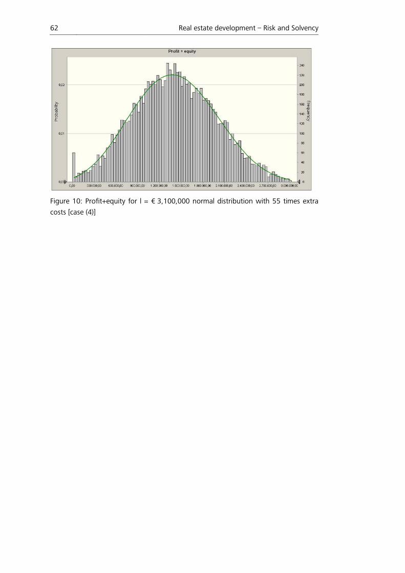
62
Figure 10: Profit+equity for l =
costs [case (4)]
Real estate development – Risk and S
= € 3,100,000 normal distribution with 55 tim
Solvency
mes extra
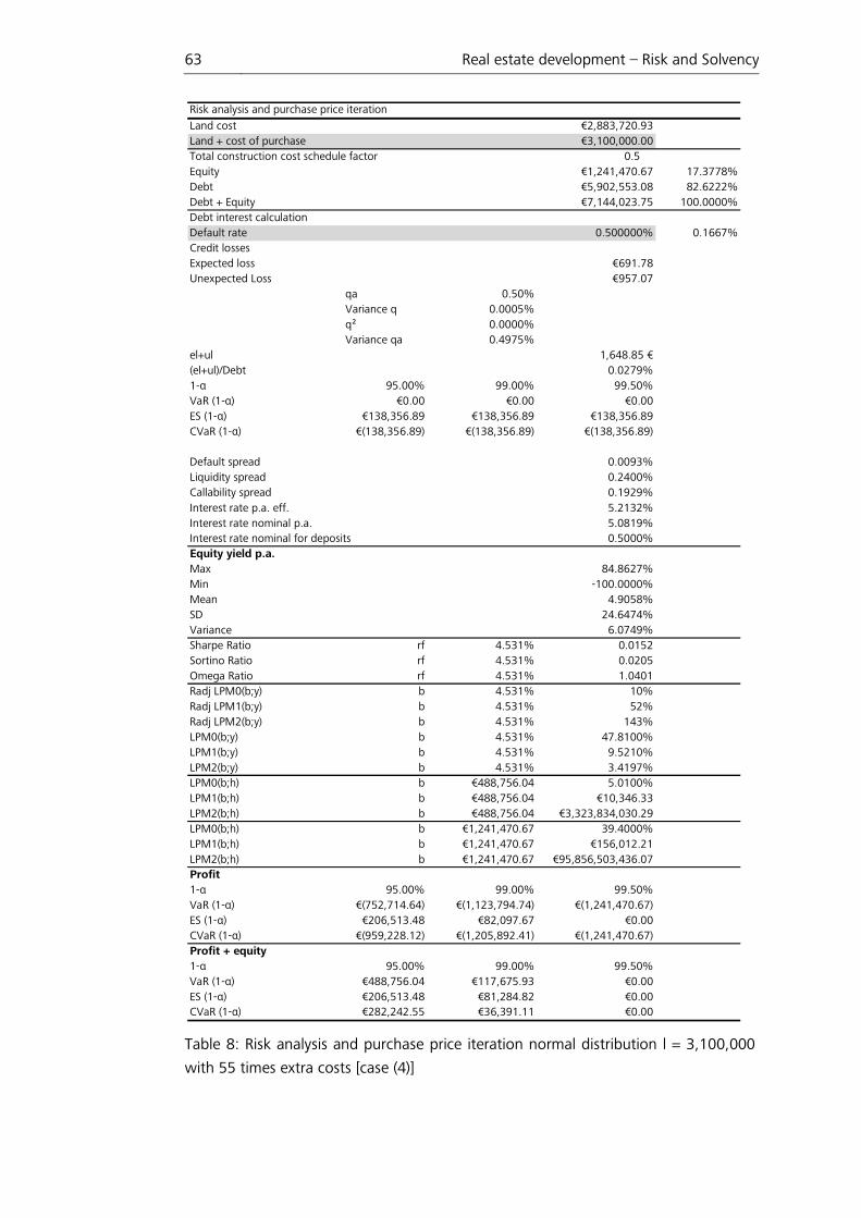
63 Real estate development – Risk and Solvency
Table 8: Risk analysis and purchase price iteration normal distribution l = 3,100,000
with 55 times extra costs [case (4)]
Risk analysis and purchase price iteration
Land cost €2,883,720.93Land + cost of purchase €3,100,000.00Total construction cost schedule factor 0.5 Equity €1,241,470.67 17.3778%Debt €5,902,553.08 82.6222%Debt + Equity €7,144,023.75 100.0000%Debt interest calculationDefault rate 0.500000% 0.1667%Credit lossesExpected loss €691.78Unexpected Loss €957.07
qa 0.50%Variance q 0.0005%q² 0.0000%Variance qa 0.4975%
el+ul 1,648.85 €(el+ul)/Debt 0.0279%1-α 95.00% 99.00% 99.50%VaR (1-α) €0.00 €0.00 €0.00ES (1-α) €138,356.89 €138,356.89 €138,356.89CVaR (1-α) €(138,356.89) €(138,356.89) €(138,356.89)
Default spread 0.0093%Liquidity spread 0.2400%Callability spread 0.1929%
Interest rate p.a. eff. 5.2132%Interest rate nominal p.a. 5.0819%
0.5000%Equity yield p.a.Max 84.8627%Min -100.0000%Mean 4.9058%SD 24.6474%Variance 6.0749%Sharpe Ratio rf 4.531% 0.0152Sortino Ratio rf 4.531% 0.0205Omega Ratio rf 4.531% 1.0401Radj LPM0(b;y) b 4.531% 10%Radj LPM1(b;y) b 4.531% 52%Radj LPM2(b;y) b 4.531% 143%LPM0(b;y) b 4.531% 47.8100%LPM1(b;y) b 4.531% 9.5210%LPM2(b;y) b 4.531% 3.4197%LPM0(b;h) b €488,756.04 5.0100%LPM1(b;h) b €488,756.04 €10,346.33LPM2(b;h) b €488,756.04 €3,323,834,030.29LPM0(b;h) b €1,241,470.67 39.4000%LPM1(b;h) b €1,241,470.67 €156,012.21LPM2(b;h) b €1,241,470.67 €95,856,503,436.07Profit1-α 95.00% 99.00% 99.50%VaR (1-α) €(752,714.64) €(1,123,794.74) €(1,241,470.67)ES (1-α) €206,513.48 €82,097.67 €0.00CVaR (1-α) €(959,228.12) €(1,205,892.41) €(1,241,470.67)Profit + equity1-α 95.00% 99.00% 99.50%VaR (1-α) €488,756.04 €117,675.93 €0.00ES (1-α) €206,513.48 €81,284.82 €0.00CVaR (1-α) €282,242.55 €36,391.11 €0.00
Interest rate nominal for deposits
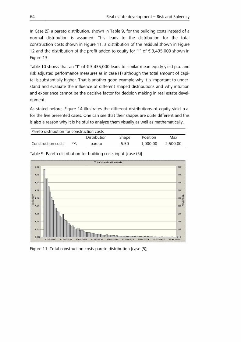
64
In Case (5) a pareto distribution
normal distribution is assum
construction costs shown in Fig
12 and the distribution of the p
Figure 13.
Table 10 shows that an “l” of €
risk adjusted performance mea
tal is substantially higher. That
stand and evaluate the influen
and experience cannot be the d
opment.
As stated before, Figure 14 illu
for the five presented cases. On
is also a reason why it is helpfu
Table 9: Pareto distribution for
Figure 11: Total construction co
Pareto distribution for construct
D
Construction costs cai
Real estate development – Risk and S
ion, shown in Table 9, for the building costs inste
med. This leads to the distribution for th
Figure 11, a distribution of the residual shown in
e profit added to equity for “l” of € 3,435,000 sh
€ 3,435,000 leads to similar mean equity yield p
easures as in case (1) although the total amount
t is another good example why it is important to
ence of different shaped distributions and why i
e decisive factor for decision making in real estat
illustrates the different distributions of equity yi
One can see that their shapes are quite different
ful to analyze them visually as well as mathemati
r building costs input [case (5)]
costs pareto distribution [case (5)]
ction costs
Distribution Shape Position Ma
pareto 5.50 1,000.00 2,500
Solvency
stead of a
the total
in Figure
shown in
d p.a. and
t of capi-
to under-
y intuition
ate devel-
yield p.a.
t and this
tically.
ax
00.00
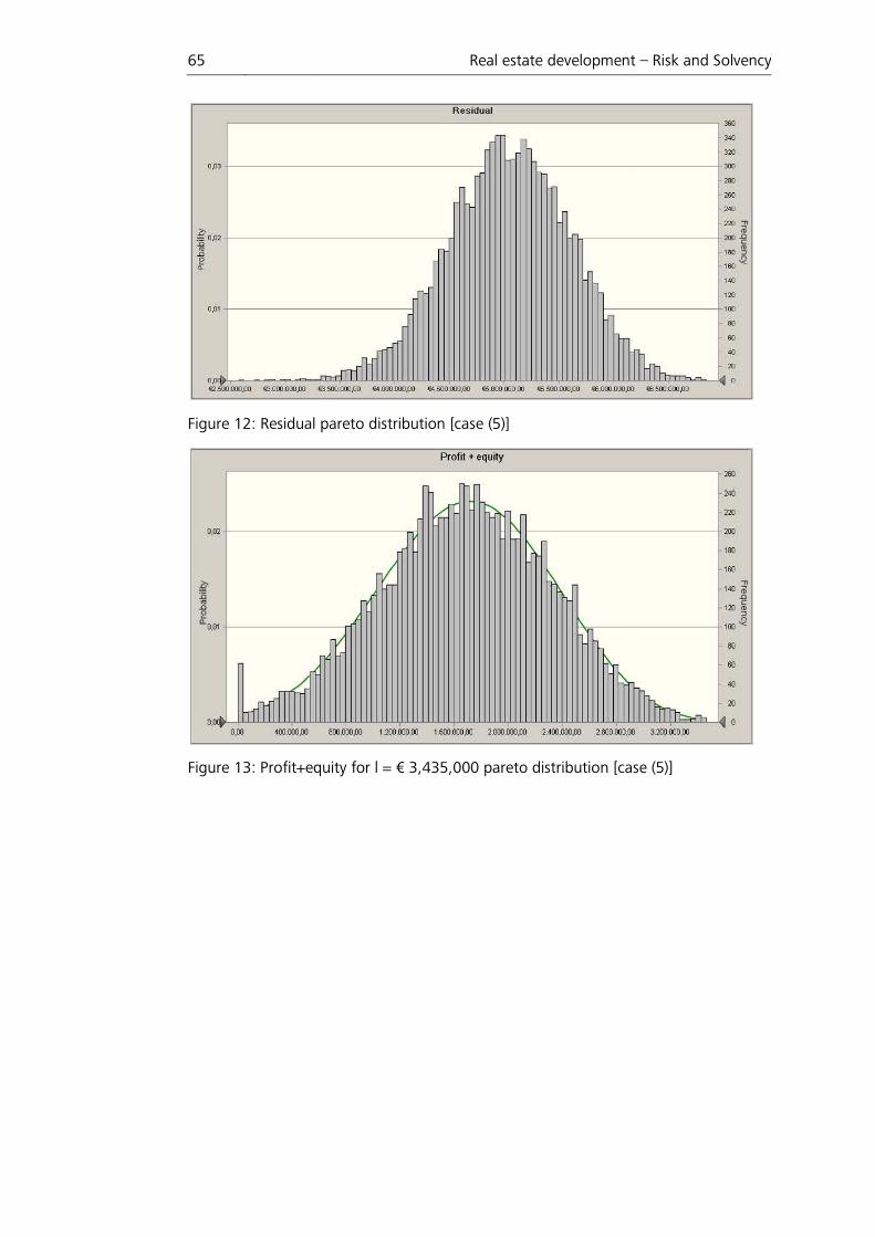
65
Figure 12: Residual
Figure 13: Profit+eq
Real estate development
pareto distribution [case (5)]
equity for l = € 3,435,000 pareto distribution [cas
nt – Risk and Solvency
ase (5)]
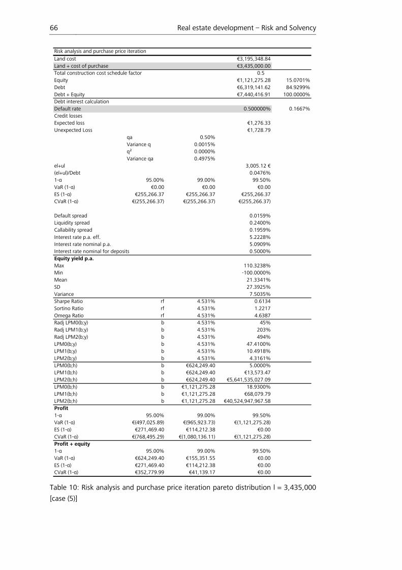
66 Real estate development – Risk and Solvency
Table 10: Risk analysis and purchase price iteration pareto distribution l = 3,435,000
[case (5)]
Risk analysis and purchase price iteration
Land cost €3,195,348.84Land + cost of purchase €3,435,000.00Total construction cost schedule factor 0.5 Equity €1,121,275.28 15.0701%Debt €6,319,141.62 84.9299%Debt + Equity €7,440,416.91 100.0000%Debt interest calculationDefault rate 0.500000% 0.1667%Credit lossesExpected loss €1,276.33Unexpected Loss €1,728.79
qa 0.50%Variance q 0.0015%q² 0.0000%Variance qa 0.4975%
el+ul 3,005.12 €(el+ul)/Debt 0.0476%1-α 95.00% 99.00% 99.50%VaR (1-α) €0.00 €0.00 €0.00ES (1-α) €255,266.37 €255,266.37 €255,266.37CVaR (1-α) €(255,266.37) €(255,266.37) €(255,266.37)
Default spread 0.0159%Liquidity spread 0.2400%Callability spread 0.1959%
Interest rate p.a. eff. 5.2228%Interest rate nominal p.a. 5.0909%
0.5000%Equity yield p.a.Max 110.3238%Min -100.0000%Mean 21.3341%SD 27.3925%Variance 7.5035%Sharpe Ratio rf 4.531% 0.6134Sortino Ratio rf 4.531% 1.2217Omega Ratio rf 4.531% 4.6387Radj LPM0(b;y) b 4.531% 45%Radj LPM1(b;y) b 4.531% 203%Radj LPM2(b;y) b 4.531% 494%LPM0(b;y) b 4.531% 47.4100%LPM1(b;y) b 4.531% 10.4918%LPM2(b;y) b 4.531% 4.3161%LPM0(b;h) b €624,249.40 5.0000%LPM1(b;h) b €624,249.40 €13,573.47LPM2(b;h) b €624,249.40 €5,641,535,027.09LPM0(b;h) b €1,121,275.28 18.9300%LPM1(b;h) b €1,121,275.28 €68,079.79LPM2(b;h) b €1,121,275.28 €40,524,947,967.58Profit1-α 95.00% 99.00% 99.50%VaR (1-α) €(497,025.89) €(965,923.73) €(1,121,275.28)ES (1-α) €271,469.40 €114,212.38 €0.00CVaR (1-α) €(768,495.29) €(1,080,136.11) €(1,121,275.28)Profit + equity1-α 95.00% 99.00% 99.50%VaR (1-α) €624,249.40 €155,351.55 €0.00ES (1-α) €271,469.40 €114,212.38 €0.00CVaR (1-α) €352,779.99 €41,139.17 €0.00
Interest rate nominal for deposits
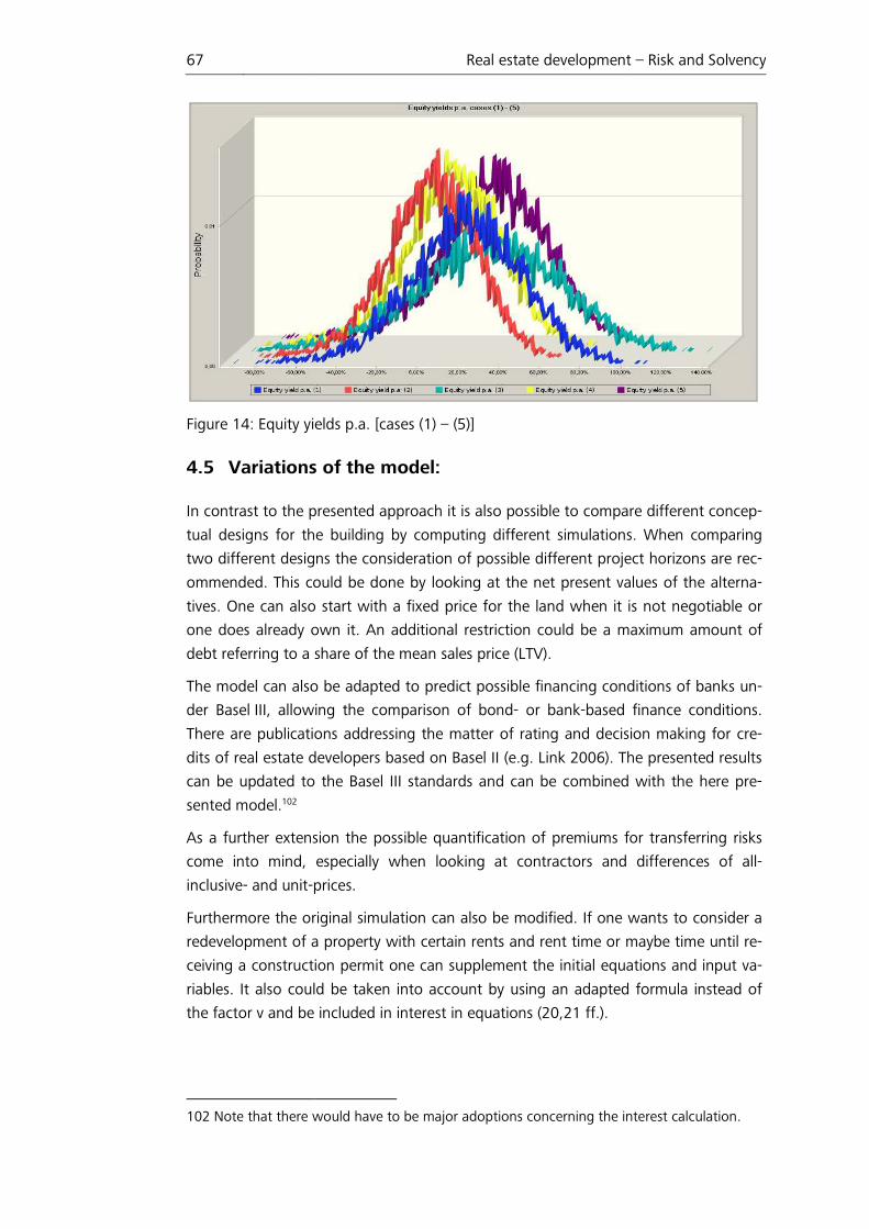
67
Figure 14: Equity yie
4.5 Variations
In contrast to the p
tual designs for th
two different desig
ommended. This co
tives. One can also
one does already o
debt referring to a s
The model can also
der Basel III, allowi
There are publicatio
dits of real estate d
can be updated to
sented model.102
As a further extens
come into mind,
inclusive- and unit-p
Furthermore the or
redevelopment of a
ceiving a constructi
riables. It also coul
the factor v and be
102 Note that there w
Real estate development
yields p.a. [cases (1) – (5)]
s of the model:
presented approach it is also possible to compar
the building by computing different simulations
igns the consideration of possible different proje
could be done by looking at the net present va
so start with a fixed price for the land when it i
own it. An additional restriction could be a m
a share of the mean sales price (LTV).
lso be adapted to predict possible financing cond
wing the comparison of bond- or bank-based
tions addressing the matter of rating and decis
developers based on Basel II (e.g. Link 2006). Th
to the Basel III standards and can be combined
nsion the possible quantification of premiums fo
, especially when looking at contractors and
prices.
original simulation can also be modified. If one w
f a property with certain rents and rent time or m
ction permit one can supplement the initial equa
uld be taken into account by using an adapted
e included in interest in equations (20,21 ff.).
would have to be major adoptions concerning the in
nt – Risk and Solvency
are different concep-
ns. When comparing
ject horizons are rec-
values of the alterna-
t is not negotiable or
maximum amount of
nditions of banks un-
d finance conditions.
ision making for cre-
The presented results
d with the here pre-
for transferring risks
d differences of all-
e wants to consider a
r maybe time until re-
uations and input va-
d formula instead of
interest calculation.
68 Real estate development – Risk and Solvency
4.6 Conclusion
Although simulation has limitations and a qualitative risk management is of high im-
portance the presented model provides an easily understandable extension to the
common residual valuation approach and the respective developer calculation. This
tool for quantitative risk management improves decision-making in favour or against
a project. It also provides the possibility to analyze and compare different finance
structures and the different components as well as project variations. Furthermore it
can be used to support the quantification of risks in the running development process
by updating it with realized inputs and by that help to ensure the solvency until the
project is finished. Possible problems can be identified in early stages and counter
measures regarding the financing can be taken.103
Simulation and estimation of simulation parameters has a higher potential for cheat-
ing than scenario or sensitivity analysis. This comes especially into account when
there is little equity involved and one is risking other people’s money. In a ZRPF the
alignment of interest might therefore only be ensured if all the partners have the
knowhow for evaluating in- and outputs of the simulation. Another limitation might
be the fact that on the short run the smarter developer might not be able to pur-
chase the projects because another developer underestimating risk might buy the site
for a higher price. On the long run this should of course lead to an elimination of the
ignorant developer but he might be replaced by a new actor with the same ignor-
ance.
103 Note that some of the formula presented might have to be adjusted if one has other limi-tations based on new inputs or realized risks.

69 Anhang
Anhang
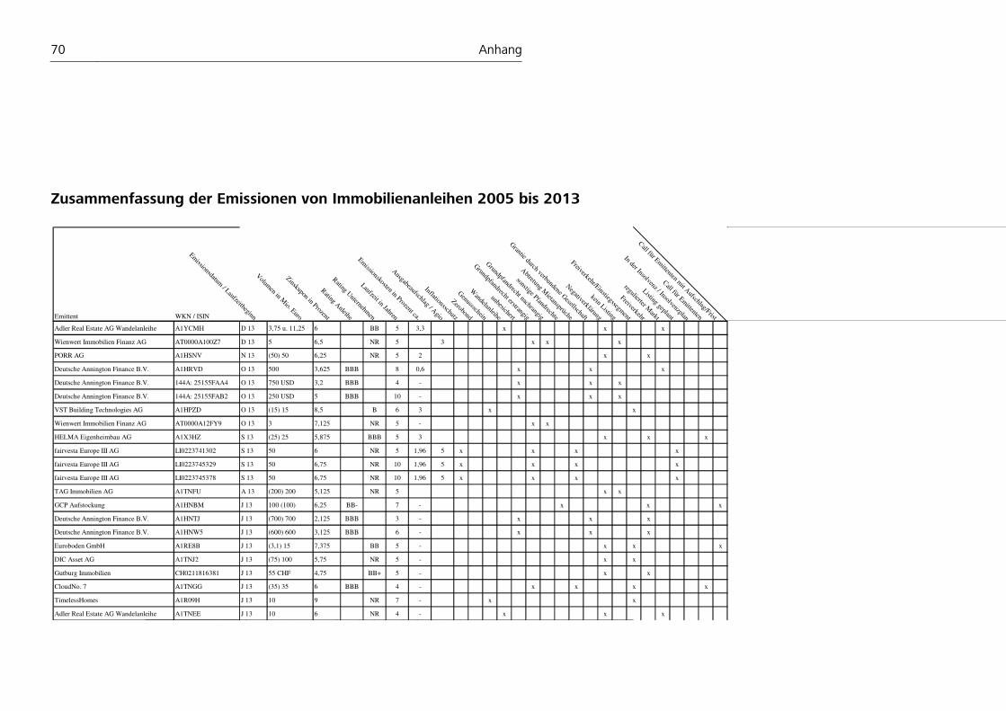
70 Anhang
Zusammenfassung der Emissionen von Immobilienanleihen 2005 bis 2013
Emittent WKN / ISIN
Emissionsdatum
/ Laufzeitbeginn
Volum
en in Mio. Euro
Zinskupon in Prozent
Rating A
nleihe
Rating U
nternehmen
Laufzeit in Jahren
Emissionskosten in Prozent ca.
Ausgabeaufschlag / A
gio
Inflationsschutz
Zerobond
Genussschein
Wandelanleihe
unbesichert
Grundpfandrecht erstrangig
Grundpfandrecht nachrangig
sonstige Pfandrechte
Abtretung M
ietansprüche
Grantie durch verbundene G
esellschaft
Negativerklärung
kein Listing
Freiverkehr/Einstiegssegment
Freiverkehr
regulierter Markt
Listing geplant
In der Insolvenz / Insolvenzplan
Call für Em
ittenten
Call für Em
ittenten mit A
ufschlag/Frist
Adler Real Estate AG Wandelanleihe A1YCMH D 13 3,75 u. 11,25 6 BB 5 3,3 x x x
Wienwert Immobilien Finanz AG AT0000A100Z7 D 13 5 6,5 NR 5 3 x x x
PORR AG A1HSNV N 13 (50) 50 6,25 NR 5 2 x x
Deutsche Annington Finance B.V. A1HRVD O 13 500 3,625 BBB 8 0,6 x x x
Deutsche Annington Finance B.V. 144A: 25155FAA4 O 13 750 USD 3,2 BBB 4 - x x x
Deutsche Annington Finance B.V. 144A: 25155FAB2 O 13 250 USD 5 BBB 10 - x x x
VST Building Technologies AG A1HPZD O 13 (15) 15 8,5 B 6 3 x x
Wienwert Immobilien Finanz AG AT0000A12FY9 O 13 3 7,125 NR 5 - x x
HELMA Eigenheimbau AG A1X3HZ S 13 (25) 25 5,875 BBB 5 3 x x x
fairvesta Europe III AG LI0223741302 S 13 50 6 NR 5 1,96 5 x x x x
fairvesta Europe III AG LI0223745329 S 13 50 6,75 NR 10 1,96 5 x x x x
fairvesta Europe III AG LI0223745378 S 13 50 6,75 NR 10 1,96 5 x x x x
TAG Immobilien AG A1TNFU A 13 (200) 200 5,125 NR 5 x x
GCP Aufstockung A1HNBM J 13 100 (100) 6,25 BB- 7 - x x x
Deutsche Annington Finance B.V. A1HNTJ J 13 (700) 700 2,125 BBB 3 - x x x
Deutsche Annington Finance B.V. A1HNW5 J 13 (600) 600 3,125 BBB 6 - x x x
Euroboden GmbH A1RE8B J 13 (3,1) 15 7,375 BB 5 - x x x
DIC Asset AG A1TNJ2 J 13 (75) 100 5,75 NR 5 - x x
Gutburg Immobilien CH0211816381 J 13 55 CHF 4,75 BB+ 5 - x x
CloudNo. 7 A1TNGG J 13 (35) 35 6 BBB 4 - x x x x
TimelessHomes A1R09H J 13 10 9 NR 7 - x x
Adler Real Estate AG Wandelanleihe A1TNEE J 13 10 6 NR 4 - x x x
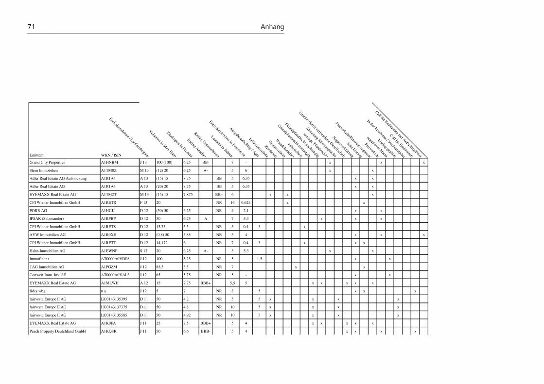
71 Anhang
Emittent WKN / ISIN
Emissionsdatum
/ Laufzeitbeginn
Volum
en in Mio. Euro
Zinskupon in Prozent
Rating A
nleihe
Rating U
nternehmen
Laufzeit in Jahren
Emissionskosten in Prozent ca.
Ausgabeaufschlag / A
gio
Inflationsschutz
Zerobond
Genussschein
Wandelanleihe
unbesichert
Grundpfandrecht erstrangig
Grundpfandrecht nachrangig
sonstige Pfandrechte
Abtretung M
ietansprüche
Grantie durch verbundene G
esellschaft
Negativerklärung
kein Listing
Freiverkehr/Einstiegssegment
Freiverkehr
regulierter Markt
Listing geplant
In der Insolvenz / Insolvenzplan
Call für Em
ittenten
Call für Em
ittenten mit A
ufschlag/Frist
Grand City Properties A1HNBM J 13 100 (100) 6,25 BB- 7 - x x x
Stern Immobilien A1TM8Z M 13 (12) 20 6,25 A- 5 6 x x
Adler Real Estate AG Aufstockung A1R1A4 A 13 (15) 15 8,75 BB 5 6,35 x x
Adler Real Estate AG A1R1A4 A 13 (20) 20 8,75 BB 5 6,35 x x
EYEMAXX Real Estate AG A1TM2T M 13 (15) 15 7,875 BB+ 6 - x x x
CPI Wiener Immobilien GmbH A1RETR F 13 20 NR 16 0,625 x x
PORR AG A1HCJJ D 12 (50) 50 6,25 NR 4 2,1 x x
IPSAK (Salamander) A1RFBP D 12 30 6,75 A 7 5,3 x x x
CPI Wiener Immobilien GmbH A1RETS D 12 13,75 5,5 NR 5 0,4 3 x
AVW Immobilien AG A1R0XE D 12 (0,8) 50 5,85 NR 3 4 x x x
CPI Wiener Immobilien GmbH A1RETT D 12 14,172 6 NR 7 0,4 3 x x x
Hahn-Immobilien AG A1EWNF S 12 20 6,25 A- 5 5,3 x x
Immofinanz AT0000A0VDP8 J 12 100 5,25 NR 5 1,5 x x
TAG Immobilien AG A1PGZM J 12 85,3 5,5 NR 7 x x
Conwert Imm. Inv. SE AT0000A0VAL3 J 12 65 5,75 NR 5 - x x
EYEMAXX Real Estate AG A1MLWH A 12 15 7,75 BBB+ 5,5 5 x x x x x
fides wbg n.a. J 12 5 7 NR 8 5 x x x
fairvesta Europe II AG LI03143135395 D 11 50 4,2 NR 5 5 x x x x
fairvesta Europe II AG LI03143137375 D 11 50 4,8 NR 10 5 x x x x
fairvesta Europe II AG LI03143135585 D 11 50 4,92 NR 10 5 x x x x
EYEMAXX Real Estate AG A1K0FA J 11 25 7,5 BBB+ 5 4 x x x x x
Peach Property Deutchland GmbH A1KQ8K J 11 50 6,6 BBB- 5 4 x x x x
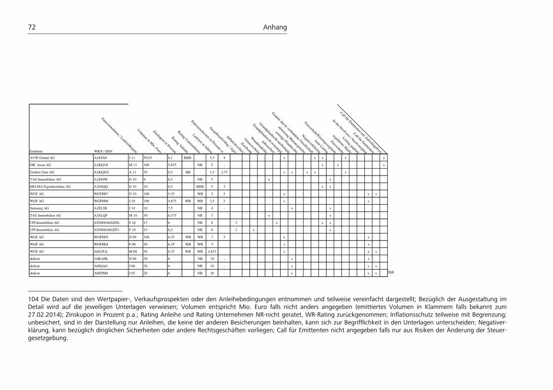
72 Anhang
104
104 Die Daten sind den Wertpapier-, Verkaufsprospekten oder den Anleihebedingungen entnommen und teilweise vereinfacht dargestellt; Bezüglich der Ausgestaltung im Detail wird auf die jeweiligen Unterlagen verwiesen; Volumen entspricht Mio. Euro falls nicht anders angegeben (emittiertes Volumen in Klammern falls bekannt zum 27.02.2014); Zinskupon in Prozent p.a.; Rating Anleihe und Rating Unternehmen NR-nicht geratet, WR-Rating zurückgenommen; Inflationsschutz teilweise mit Begrenzung; unbesichert, sind in der Darstellung nur Anleihen, die keine der anderen Besicherungen beinhalten, kann sich zur Begrifflichkeit in den Unterlagen unterscheiden; Negativer-klärung, kann bezüglich dinglichen Sicherheiten oder andere Rechtsgeschäften vorliegen; Call für Emittenten nicht angegeben falls nur aus Risiken der Änderung der Steuer-gesetzgebung.
Emittent WKN / ISIN
Emissionsdatum
/ Laufzeitbeginn
Volum
en in Mio. Euro
Zinskupon in Prozent
Rating A
nleihe
Rating U
nternehmen
Laufzeit in Jahren
Emissionskosten in Prozent ca.
Ausgabeaufschlag / A
gio
Inflationsschutz
Zerobond
Genussschein
Wandelanleihe
unbesichert
Grundpfandrecht erstrangig
Grundpfandrecht nachrangig
sonstige Pfandrechte
Abtretung M
ietansprüche
Grantie durch verbundene G
esellschaft
Negativerklärung
kein Listing
Freiverkehr/Einstiegssegment
Freiverkehr
regulierter Markt
Listing geplant
In der Insolvenz / Insolvenzplan
Call für Em
ittenten
Call für Em
ittenten mit A
ufschlag/Frist
AVW Grund AG A1E8X6 J 11 50,83 6,1 BBB- 5,5 4 x x x x x
DIC Asset AG A1KQ1N M 11 100 5,875 NR 5 - x x x
Golden Gate AG A1KQXX A 11 30 6,5 BB 3,5 2,75 x x x x x
TAG Immobilien AG A1E89W D 10 9 6,5 NR 5 x x
HELMA Eigenheimbau AG A1E8QQ D 10 10 6,5 BBB 5 3 x x
WGF AG WGFH07 N 10 100 5,35 WR 5 3 x x x
WGF AG WGFH06 J 10 100 4,875 WR WR 2,5 3 x x
Samonig AG A1EL5B J 10 10 7,5 NR 4 - x x
TAG Immobilien AG A1ELQF M 10 30 6,375 NR 5 x x
CPI Immobilien AG AT0000A0GZE6 F 10 15 6 NR 8 3 x x x
CPI Immobilien AG AT0000A0GZF3 F 10 15 6,5 NR 8 3 x x
WGF AG WGFH05 D 09 100 6,35 WR WR 7 5 x x
WGF AG WGFH04 F 09 50 6,35 WR WR 5 x x
WGF AG A0LDUL M 08 50 6,35 WR WR 4,833 x x x
deikon A0KAHL N 06 30 6 NR 10 - x x
deikon A0JQAG J 06 20 6 NR 10 - x x x
deikon A0EPM0 J 05 20 6 NR 10 - x x x
73 Literatur
Literatur
Ahlswede, S./Just, T. (2010), Refinanzierungsrisiken bei Gewerbeimmobiliendarlehen:
CMBS sind nur ein Teil eines wachsenden Problems, Deutsche Bank Research.
Almond, N. (2012), Global Debt Funding Gap – New non-bank lending offsets EBA
impact, DTZ Insight, DTZ Research.
Almond, N./Vrensen H. (2013), Net Debt Funding Gap – Non-banks trigger surplus in
core Europe, DTZ Insight, DTZ Research.
Alram, J./Schalast, C. (2009), Konstruktion einer Anleihe mit hypothekarischer Besi-
cherung, Frankfurt School of Finance and Management Working Paper Series, Nr.
113, Frankfurt am Main.
Altmeppen, H.; F. Brauer (2009): Den Fair Value fairer machen, Immobilien & Finanzie-
rung, Vol. 22, pp. 10-12.
Amato, J.D. and Remolona, E.M. (2005). The pricing of unexpected credit losses. BIS
Working paper, 190, 162-182.
Atherton, E., French, N. and Gabrielli, L. (2008). Decision theory and real estate devel-
opment: a note on uncertainty. Journal of European Real Estate Research, 1, 162-
182. doi: 10.1108/17539260810918730
BCG (2010), BCG Risk Report 2010 - Facing New Realities in European Banking, Risk
Management after the Crisis and Impact of Basel III, Boston.
Benston, G. J./Smith, C. W. S. Jr. (1976), The Journal of Finance, 31. Jg., Nr. 2, S. 215-
231.
Bohn, T., Wiedenmann, M. and Wagner, J. (2002). Datenanalyse und Auswertung:
Risiken bei der Immobilienprojektentwicklung [Data analysis and evaluation: risks as-
sociated with real estate project development]. In Wiedenmann M. (2005), Risikoma-
nagement bei der Immobilien-Projektentwicklung unter besonderer Berücksichtigung
der Risikoanalyse und Risikoquantifizierung, Schriftenreihe Institut für Stadtentwick-
lung und Bauwirtschaft Universität Leipzig, 8, Nordersted: Books on Demand GmbH.
Brückner, D. (2011), Ein Joint Venture hilft, das Eigenkapital zu vergrößern, Immobi-
lienzeitung, 18. Jg., Nr. 6, S. 13.
Brückner, D./de Boer A. (2011), Alles anders, alles gleich Die Finanzierung durch Im-
mobilienanleihen am Kapitalmarkt, GoingPublic Magazin, 14. Jg., Sonderausgabe Ka-
pitalmarktrecht, S. 68-69.
Bundesbank (2013), Basisdaten 2010-2013, in:
http://www.bundesbank.de/Redaktion/DE/Standardartikel/Statistiken/FSI/fsi_basisdate
n_2010_2013.html?searchArchive=0&submit=Suchen&searchIssued=0&templateQuer
yString=basisdaten, abgerufen am 2. Dezember 2013.

74 Literatur
Cloud No7 GmbH (2013), Wertpapierprospekt A1TNGG, in: http://www.cloudno7-
anleihe.de/pdf/Wertpapierprospekt_Cloud_No_7_GmbH_10062013.pdf, abgerufen
am 9. Februar 2014.
Crosby, N. (2007): German Open Ended Funds: Was there a valuation problem? Work-
ing Paper in Real Estate & Planning 05/07, University of Reading.
Crosby, N., C. Lizieri and P. McAllister (2009): Means, Motive and Opportunity? Disen-
tangling Client Influence on Performance Measurement Appraisals, Paper presented at
the European Real Estate Society conference, Stockholm, Sweden.
Deutsche Annington B.V. (2013a), Base Prospectus, in: http://www.wertpapier-
forum.de/index.php?app=core&module=attach§ion=attach&attach_id=81407,
abgerufen am 26. Februar 2014.
Deutsche Annington B.V. (2013b), Wertpapierprospekt A1HRVD, in:
http://www.wertpapier-
forum.de/index.php?app=core&module=attach§ion=attach&attach_id=81408,
abgerufen am 25. Februar 2014.
Downie, M.L., Schulte, K.-W.; Thomas, M. (1996): Germany, in Adair A., Downie. M.
L., McGreal, S. and Vos, G. (eds): European Valuation Practice, Theory and Tech-
niques, E. & F.N. Spon, London.
Drukarczyk, J. (2008), Finanzierung, 10. Auflage, Stuttgart.
Drukarczyk, J. (2008). Finanzierung [Financing] (10th ed.). Stuttgart: Lucius & Lucius.
Engel, R. (2002): Das Aus für die DCF-Methode?, Grundstücksmarkt und Grund-
stückswert 13 (6), pp. 321-332.
Esty, B. C. (2004). Modern Project Finance: A Casebook (1st ed.). Boston: John Wiley &
Sons Inc..
French, N. (2003): The RICS valuation and appraisal standards, Journal of Property In-
vestment and Finance, 21(6), pp. 495-501.
GDV (2011), GDV Positionspapier Auswirkungen von Solvency II auf die Kapitalanla-
gen der deutschen Versicherungsunternehmen.
Gehner, E., Halman, J.I.M. and de Jonge H. (2006). RISK MANAGEMENT IN THE
DUTCH REAL ESTATE DEVELOPMENT SECTOR: A SURVEY. Retrieved from:
www.irbnet.de/daten/iconda/CIB9048.pdf
Gimplevich, D. (2010). Simulation-based excess return model for real estate develop-
ment: A practical Monte Carlo simulation-based method for quantitative risk man-
agement and project valuation for real estate development projects illustrated with a
high-rise office development case study. Journal of Property Investment & Finance,
29, 115 – 144. doi: 10.1108/14635781111112765
Gläsner, S.M.; Thomas, M.; Schiereck, D. (2010): Lack of German Real Estate Fund
Volatility – is the Market or the Valuer to Blame, in: Gläsner, S. M. (2010): Return Pat-
75 Literatur
terns of German Open-End Real Estate Funds - An Empirical Explanation of Smooth
Fund Returns, Frankfurt: Peter Lang, pp. 35-56.
Gleißner, W. and Wiegelmann, T. (2012). Quantitative methods for risk management
in the real estate development industry. Journal of Property Investment & Finance,
30(6), pp. –.
Graalmann, B. (2011), Basel III und die Immobilienfinanzierung, Immobilienmanager,
21. Jg., Nr. 2, S. 15-17.
Härle P. et al. (2010), Basel III and European banking: Its impact, how banks might re-
spond, and the challenges of implementation, McKinsey Working Papers on Risk, Nr.
26.
Haugwitz, L. (2012), Kreditklemme - bis 2015 oder länger?, Immobilien & Finanzie-
rung, 12. Jg., Nr. 23, S. 853.
Hesse, M./Just, T. (2013), IREBS GERMAN DEBT PROJECT – Analyse des deutschen
Marktes für gewerbliche Immobilienfinanzierung, IREBS Institut für Immobilienwirt-
schaft, Regensburg.
Hinrichs/Schultz (2003): Das Discounted–Cash-Flow-Verfahren in der Praxis, Grund-
stücksmarkt und Grundstückswert, 14(5), pp. 265-272.
Holthaus, U. (2007). Ökonomisches Model mit Risikobetrachtung für die Projektent-
wicklung: Eine Problemanalyse mit Lösungsansätzen [Economic model with risk as-
sessment for project development: An analysis of problems with solutions]. Fakultät
für Bauwesen Universität Dortmund. Retrieved from: https://eldorado.tu-
dortmund.de/bitstream/2003/24284/5/holthaus2.pdf
Horn, H.-J. (2003): Der europäische Sachverständigenverband TEGoVA, Immobilien &
Finanzierung, No.13, pp. 24-26.
Horsch, A/Sturm, S. (2007), Disintermediation durch Mikroanleihen, Kredit und Kapi-
tal, 40. Jg., Nr. 2, S. 265-315.
Houweling, P., Mentink, A., Vorst T. (2003). How to measure corporate bond liquid-
ity? Tingbergen Institute Discussion Paper, 30(2), 1-34.
Hughes, F./Moss, A. (2011), Finding the Right Blend - Part II, EPRA News, S. 15-21.
Kalotay, A. J., Williams, G.O., Fabozzi, F.J. (1993). A Model for Valuing Bonds and
Embedded Options. Financial Analysts Journal, 49(3), 35-46.
Kaplan, P. D. and Knowles, J. A. (2004). Kappa: A Generalized Downside Risk-
Adjusted Performance Measure, Journal of Performance Measurement, 8 (3).
Katzung, N. (2013), Risiko Mittelstandsanleihe, in: http://www.immobilien-
zeitung.de/122821/risiko-mittelstandsanleihe, abgerufen am 5. November 2013.
Kilbinger, S.S. (2006): Run on German Real Estate Funds Exposes Flows in Regulation,
Wall Street Journal online, www.realestatejournal.com/reits/20060131-kilbinger.html.
76 Literatur
Kleiber (2009): § 18 ImmoWertVO, in: Kleiber, W., Simon, J., Weyers, G., Schröter, K.
(eds.): „Verkehrswertermittlung von Grundstücken“, 6st edition, 2010, Bundesanzei-
gerverlag, Köln
Kleiber, W. (2004): Was sind eigentlich internationale Bewertungsverfahren? Grund-
stücksmarkt und Grundstückswert, 15(6), pp. 193-207.
Kleiber, W. (2007): Ertragswertermittlung verlangt "prophetische Gaben", Immobilien-
zeitung, Nr.18, p. 8.
Kleiber, W., Simon, J. and Weyers, G (1994): Verkehrswertermittlung von Grundstü-
cken, 2nd edition, 1994, Bundesanzeigerverlag, Köln
Leland, H./Pyle, D. (1977), Informational Symmetries, Financial Structure and Financial
Intermediation, The Journal of Finance, 32. Jg., Nr.2, S. 371-387.
Levy, D. and E. Schuck (2005): The Influence of Clients on Valuations: The Clients' Per-
spective, Journal of Property Investment & Finance 23(2), pp. 182-201.
Leykam, M. (2014), Anlegeranwalt Dittke verklagt WGF-Führung, in:
http://www.immobilienzeitung.de/1000018577/anlegeranwalt-dittke-verklagt-wgf-
fuehrung, abgerufen am 26. Februar 2014.
Link, A. (2006). Rating und Kreditentscheidungsmodell für Immobilien-
Projektentwicklungen [Rating and credit decision model for real estate development
projects]. Banking & Finance aktuell, Band 25, Frankfurt am Main
Loizou, P. and French, N., (2012). Risk and uncertainty in development: A critical
evaluation of using the Monte Carlo simulation method as a decision tool in real es-
tate development projects. Journal of Property Investment & Finance, 30, 198-210.
doi: 10.1108/14635781211206922
Loritz, K.-G. (2010), Anleihen von Immobilienunternehmen – Sicherheit ohne Ratings,
Der Immobilienbrief, 21.11.2010, in: http://www.rohmert-
medien.de/immobilienbrief/anleihen-von-immobilienunternehmen-sicherheit-ohne-
ratings,109203.html, abgerufen am 22. November 2013.
Loritz, K.-G. (2011), Immobilien-Anleihen als zeitgemäße Alternative zu geschlossenen
Fonds – Funktionsweise, rechtliche, wirtschaftliche und sicherheitsbezogene Aspekte.
In: Schmider, K.-H./Wagner, K.-R./Loritz, K.-G. (Hrsgb.) Handbuch der Bauinvestition
und Immobilienkapitalanlage, 91. Aktualisierung, S. 1-41.
MacFarlane, J. (1995). The use of simulation in property investment analysis, Journal
of Property Valuation & Investment, 13, 25-38. doi: 10.1108/14635789510099427
Mansfield, J. R., D. P. Lorenz, (2004): Shaping the future: The impacts of evolving in-
ternational accounting standards on calculation practice in the UK and Germany, in:
Property Management, 22(4), pp. 289-303.
McParl and, C., A. Adair, and S. McGreal (2002): Valuation Standards - A comparison
of four European countries. Journal of Property Investment an Finance, 20(2), pp.
127-141.
77 Literatur
Morgan, J.F.W.; Harrop, M. J. (1991): Neue Ansätze der Bewertung und Beurteilung
von Anlageobjekten, in: Grundstücksmarkt und Grundstückswert, 2 (3), pp. 128-132.
Moshammer, W. (2000): Angelsächsisch ist nicht international, Immobilienzeitung
No. 1, 2/2000, 13.01.2000, 8.
Naubereit, Philipp (2008): Standard Ground Value in the Context of the Harmoniza-
tion of Property Valuation, The Appraisal Journal, Summer, pp. 211-218.
Ong, M. K. (1999). Internal Credit Risk Models: Capital Allocation and Performance
Measurement. London: Risk Books.
Pitschke, C. (2004), Die Finanzierung gewerblicher Immobilienprojektentwicklungen
unter Basel II, Köln.
Pitschke, C. and Bone-Winkel, S. (2006). The impact of the New Basel Capital Accord
on real estate developers. Journal or Property Investment and Finance, 24, 7-26.
doi: 10.1108/14635780610642953
Rehkugler, H./Schindler F. (2012), Neue Regulierungen für die Finanzwirtschaft –
Mögliche Auswirkungen von Solvency II und Basel III für die Attraktivität von Immobi-
lienanlagen und die Immobilienfinanzierung, Betriebswirtschaftliche Forschung und
Praxis, 64 Jg., Nr. 2, S. 105-120.
Rüchardt, Konrad (1991): Bemerkungen zur Immobilienbewertung in Deutschland und
Großbritannien, Grundstücksmarkt und Grundstückswert, 2(5), pp. 128-132.
Rudolph, B. (2006), Unternehmensfinanzierung und Kapitalmarkt, Tübingen.
Samonig AG (2011), Pressemitteilung 02. Februar 2011, in: http://www.immobilien-
kapitalanlage.com/presse/samonig-ag-erste-immobilienanleihe-fuer-energetische-
sanierung/, abgerufen am 25. Februar 2014.
Schnaidt, T. and Sebastian, S. (2012). German valuation: review of methods and legal
framework. Journal or Property Investment and Finance, 30, 145-158.
doi:10.1108/14635781211206896
Schützle, J. (2011), Neue Aspekte in der Projektentwicklung. In: University of Zurich -
Center for Urban & Real Estate Management (Hrsg.), Immobilienwirtschaft aktuell:
Beiträge zur immobilienwirtschaftlichen Forschung 2010, Zürich, S. 125-136.
Simon, J. (2000): Europäische Standards für die Immobilienbewertung, Grundstücks-
markt und Grundstückswert, 11(3), pp. 134 – 141.
Simon, Jürgen (2006), Internationale Bewertungsstandards, Grundstücksmarkt und
Grundstückswert, 17(5), pp. 270-281.
Süchting, J./Paul S. (1998), Bankmanagement, 4. Auflage, Stuttgart.
Thomas (1995), M., Income Approach versus Ertragswertverfahren, Grundstücksmarkt
und Grundstückswert, 6(2), pp.35-38.
Thomesczek, H. (2012), Wellenbrecher im Bau, Immobilienmanager, 22. Jg., Nr. 06,
S. 22-23.
78 Literatur
Vogel, H. G. (2013), Der Rechtsschutz der Schuldverschreibungsgläubiger. In: Baums
(Hrsg.), Das neue Schuldverschreibungsrecht, Berlin (zugleich: Working Paper Nr. 137
des Institute for Law and Finance (ILF), Frankfurt am Main 2013).
Volquarts, M. and Radner , P. (2011). Finanzierungsalternativen für die deutsche Im-
mobilienwirtschaft: Relevanz und Marktstruktur [Financing alternatives for the Ge-
rman real estate industry: Relevance and market structure]. EBS Diskussionspapiere
zur Immobilienwirtschaft, 2, 1-57.
Volquarts, M./Radner , P. (2011), Finanzierungsalternativen für die deutsche Immobi-
lienwirtschaft, Relevanz und Marktstruktur, EBS Diskussionspapiere zur Immobilien-
wirtschaft, Nr. 2.
Walsh, P. M. (2008). Zero Recourse Project Finance: Modell zur Risikostrukturierung
von Immobilienentwicklungen [Zero-recourse Project Finance: Model for risk structur-
ing of real estate developments]. Göttingen: Sierke Verlag.
Weistroffer, C. (2010): The German open end fund crisis A valuation problem?, un-
published working paper.
WGF AG (2010), Wertpapierprospekt WGFH07, in: http://www.anleihen-finder.de/wp-
content/uploads/2012/12/WGF-Wertpapierprospekt-2010-09-17.pdf, abgerufen am
09. Februar 2014.
WGF AG (2012), Geänderter Jahresabschluss Geschäftsjahr 2009, in:
www.bundesanzeiger.de, abgerufen am 26. Februar 2014.
WGF AG (2013), Insolvenzplan AZ 504 IN 269/12, in: http://www.wgfag.de/fileadmin
/user_upload/GeschBereich/Insolvenzplan_Rechtskraft_18072013.pdf, abgerufen am
26. Februar 2014.
Wiedenmann, M. (2005). Risikomanagement bei der Immobilien-Projektentwicklung
unter besonderer Berücksichtigung der Risikoanalyse und Risikoquantifizierung [Risk
management in real estate project development with special consideration of risk
analysis and risk quantification]. Schriftenreihe Institut für Stadtentwicklung und Bau-
wirtschaft Universität Leipzig, 8, Norderstedt: Books on Demand GmbH.
Wiegelmann, T.W. (2012), Risk Management in the Real Estate Development Indus-
try: Investigations into the application of risk management concepts in leading Euro-
pean real estate development organisations. Institute of Sustainable Development &
Architecture, Bond University, Australia. Retrieved from:
http://epublications.bond.edu.au/theses/67/
Yu, F. (2005), Accounting transparency and the term structure of credit spreads, Jour-
nal of Financial Economics, 75. Jg., S. 53-84.
Zähres, M. (2011), Solvency II und Basel III Wechselwirkung beachten, dbresearch.
79 Literatur
Legal sources
Baugesetzbuch: Baugesetzbuch in der Fassung der Bekanntmachung vom 23. Sep-
tember 2004 (BGBl. I S. 2414), das zuletzt durch Artikel 4 des Gesetzes vom 31. Juli
2009 (BGBl. I S. 2585) geändert worden ist.
Pfandbriefgesetz: Pfandbriefgesetz vom 22. Mai 2005 (BGBl. I S. 1373), das zuletzt
durch Artikel 6 des Gesetzes vom 31. Juli 2009 (BGBl. I S. 2512) geändert worden ist
Investmentgesetz: Investmentgesetz vom 15. Dezember 2003 (BGBl. I S. 2676), das
zuletzt durch Artikel 10 des Gesetzes vom 8. April 2010 (BGBl. I S. 386) geändert
worden ist.
ImmoWertV: Verordnung über die Grundsätze für die Ermittlung der Verkehrswerte
von Grundstücken (Immobilienwertermittlungsverordnung - ImmoWertV); Bundesrat
Drucksache 296/09, 03.04.09,
http://www.sprengnetter.de/send_file.php/material/0296-09.pdf (July 8th, 2010).


Universität Regensburg
IREIBS Institut für Immobilienwirtschaft
Fakultät für Wirtschaftswissenschaften