AAllmmaa MMaatteerr SSttuuddiioorruumm –– UUnniivveerrssiittàà ddii BBoollooggnnaa

DOTTORATO DI RICERCA IN

BIODIVERSITA’ ED EVOLUZIONE

Ciclo XXIII

Settore scientifico-disciplinare di afferenza: BIO/05 ZOOLOGIA

MOLLUSCS OF THE MARINE PROTECTED AREA “SECCHE DI TOR PATERNO”

Presentata da: Dott. Paolo Giulio Albano

Coordinatore Dottorato Relatore Prof.ssa Barbara Mantovani Prof. Francesco Zaccanti

Co-relatore Prof. Bruno Sabelli

Esame finale anno 2011

to Ilaria and Chiara, my daughters

This PhD thesis is the completion of a long path from childhood amateur conchology to scientific research. Many people were involved in this journey, but key characters are three. Luca Marini, director of “Secche di Tor Paterno” Marine Protected Area, shared the project idea of field research on molluscs and trusted me in accomplishing the task. Without his active support in finding funds for the field activities this project would have not started. It is no exaggeration saying I would not have even thought of entering the PhD without him. Bruno Sabelli, my PhD advisor, is another person who trusted me above reasonable expectations. Witness of my childhood love for shells, he has become witness of my metamorphosis to a researcher. Last, but not least, Manuela, my wife, shared my objectives and supported me every single day despite the family challenges we had to face. Many more people helped profusely. I sincerely hope not to forget anyone. Marco Oliverio, Sabrina Macchioni, Letizia Argenti and Roberto Maltini were great SCUBA diving buddies during field activities. Betulla Morello, former researcher at ISMAR-CNR in Ancona, was my guide through the previously unexplored land of non-parametric multivariate statistics. Philippe Bouchet and Philippe Maestrati, Muséum National d'Histoire Naturelle (Paris), were welcoming and helpful during my work with them. Navigating through 23.000 specimens of Indo-Pacific triphorids from their research campaigns has been an experience I will never forget. It is rare to have so much material of excellent quality to study. I have been able to touch biodiversity first hand. Paolo Vestrucci and Roberto Colzani manage NIER Ingegneria Spa. Working with this company allowed the first contacts and activities with the Marine Protected Area which then developed into the survey that gave most of the data for this thesis. Paolo Giuntarelli, former director of the public body RomaNatura which manages the Marine Protected Area, kept on the work done by Luca Marini in safe-guarding funds for the field activities during Luca’s absence. Paolo & Marisa, Gabriella & Vincenzo were great in helping me combining work and family. Moreover, Gabriella was supportive and was one of the people who shared my objectives most. Francesca Evangelisti, Eimi Ailen Font, Michela Kuan, Wanda Moshfegh, Linda Tragni, Francesca Orrù, Maria Teresa Greco helped sorting samples out in the field or in laboratory. Anna Maria Candela, Department of Matematics, University of Bari, helped reviewing the English of some mathematical methodological parts. Mirco Travaglini and Stefania Brunetti, Library of the Department of Experimental Evolutionary Biology, helped in locating and obtaining literature. Further help during these three years has been given by Francesco Criscione, Carlo Froglia, Maria Cristina Gambi, Giuliana Gillone, Virginie Héros, Susan M. Kidwell, Constantine Mifsud, Stefano Palazzi, Paul Sammut, Cristiano Solustri, Helmut Zibrowius.

Key-words: Mollusca, ecology, biodiversity, conservation, Posidonia oceanica, coralligenous, detritic pools, Secche di Tor Paterno

1

1 Index 1  Index .......................................................................................................................................................... 1 2  Executive summary ................................................................................................................................... 5 

2.1  The molluscan diversity..................................................................................................................... 5 2.2  Biocoenoses characterization ............................................................................................................ 5 2.3  Analysis of the Posidonia leaves species assemblage ....................................................................... 5 2.4  Analysis of the Posidonia rhizomes species assemblage ................................................................... 6 2.5  Analysis of the coralligenous species assemblage ............................................................................. 6 2.6  Analysis of the detritic species assemblage ....................................................................................... 7 2.7  Agreement between death and living assemblages ........................................................................... 7 

3  Introduction ............................................................................................................................................... 9 3.1  The studied area ................................................................................................................................. 9 3.2  Why sampling in a marine protected area?...................................................................................... 11 3.3  The molluscan fauna ........................................................................................................................ 11 3.4  Abbreviations .................................................................................................................................. 12 

4  Materials and methods ............................................................................................................................. 13 4.1  Field activity .................................................................................................................................... 13 4.2  Laboratory sorting ........................................................................................................................... 15 4.3  Data analysis techniques .................................................................................................................. 15 

4.3.1  Standardisation ........................................................................................................................ 16 4.3.2  Transformation ........................................................................................................................ 16 4.3.3  Similarity matrix ...................................................................................................................... 16 4.3.4  One-way ANalysis Of VARiance (ANOVA) .......................................................................... 17 4.3.5  Mann–Whitney U test .............................................................................................................. 18 4.3.6  Cluster analysis ........................................................................................................................ 18 4.3.7  Non-metric Multi-Dimensional Scaling (MDS) ...................................................................... 19 4.3.8  Multivariate ANalysis Of SIMilarities (ANOSIM) ................................................................. 19 4.3.9  SIMilarity PERcentage breakdown (SIMPER) ....................................................................... 20 4.3.10  PERmutational Multivariate ANalysis Of VAriance (PERMANOVA) .................................. 21 

4.4  Biodiversity indices ......................................................................................................................... 21 4.4.1  Number of species (S) ............................................................................................................. 21 4.4.2  Number of specimens (N) ........................................................................................................ 22 4.4.3  Margalef’s species richness (d) ............................................................................................... 22 4.4.4  Shannon index (H’) ................................................................................................................. 22 4.4.5  Equitability (J’) ........................................................................................................................ 22 4.4.6  Simpson index (λ) .................................................................................................................... 22 

4.5  Biodiversity estimators .................................................................................................................... 23 4.6  Trophic groups and feeding guilds .................................................................................................. 23 4.7  The role of species in describing biocoenoses ................................................................................. 24 

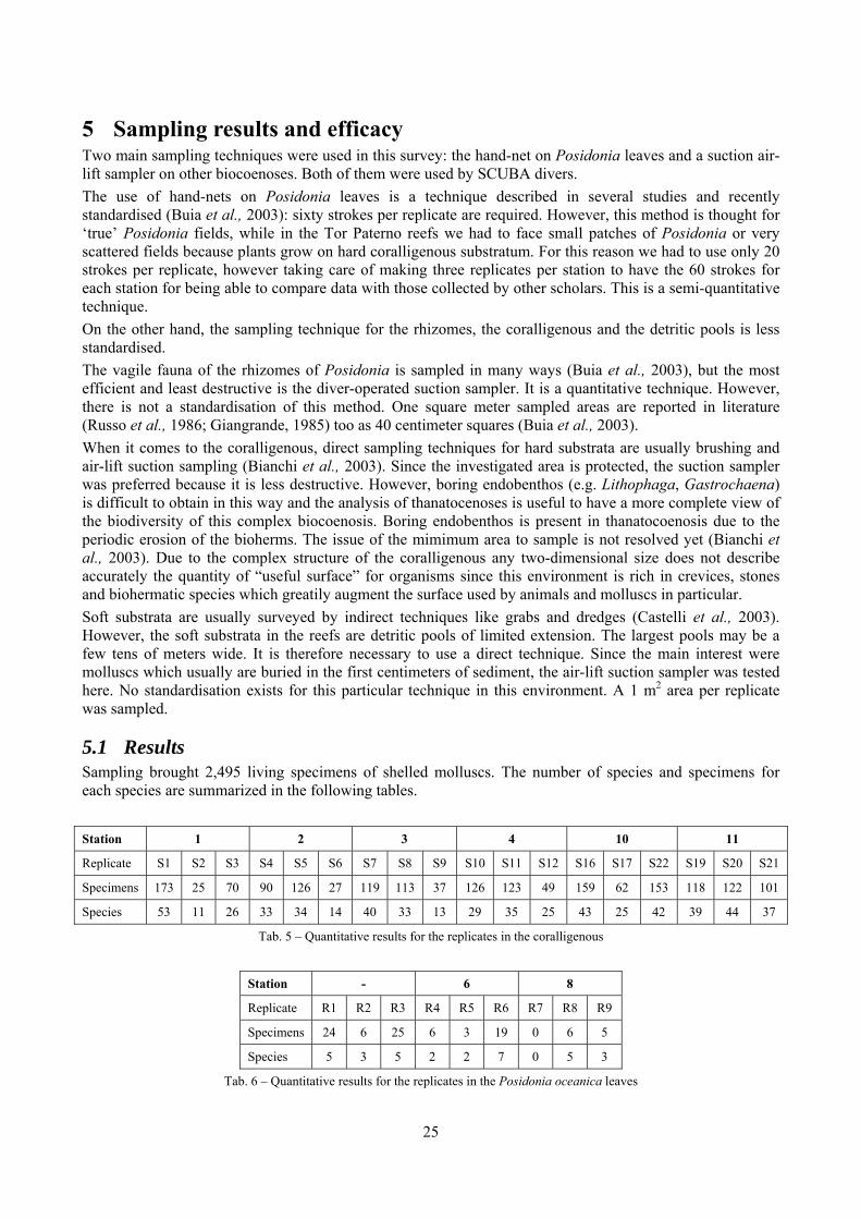
5  Sampling results and efficacy .................................................................................................................. 25 5.1  Results ............................................................................................................................................. 25 5.2  Discussion ........................................................................................................................................ 29 

6  The molluscan diversity .......................................................................................................................... 30 

2

6.1  Results ............................................................................................................................................. 30 6.1.1  Faunal list ................................................................................................................................ 30 6.1.2  Biocenotic preferences ............................................................................................................ 34 

6.2  Discussion ........................................................................................................................................ 39 6.2.1  Biodiversity of the malacofauna and its interest for conservation ........................................... 39 6.2.2  Biocenotic preferences ............................................................................................................ 43 

7  Biocoenoses characterization .................................................................................................................. 45 7.1  Results ............................................................................................................................................. 45 

7.1.1  Univariate approach ................................................................................................................. 45 7.1.2  Multivariate approach .............................................................................................................. 54 7.1.3  Analysis with other phyla ........................................................................................................ 67 

7.1.3.1  Errant Polychaeta ................................................................................................................. 67 7.1.3.2  Crustacea: “crabs” (suborder Pleocyemata) ........................................................................ 69 7.1.3.3  Brachiopoda ......................................................................................................................... 70 

7.2  Discussion ........................................................................................................................................ 71 7.2.1  Molluscs .................................................................................................................................. 71 7.2.2  Other phyla .............................................................................................................................. 73 

8  Analysis of the Posidonia leaves species assemblage ............................................................................. 74 8.1  Results ............................................................................................................................................. 74 

8.1.1  Posidonia oceanica bed structure and morphometry .............................................................. 74 8.1.2  The molluscan community ...................................................................................................... 76 8.1.3  Mollusca community structure ................................................................................................ 78 8.1.4  Comparison with other data sets .............................................................................................. 80 

8.1.4.1  Secche della Meloria (Livorno) ........................................................................................... 82 8.1.4.2  Elba Isl. ................................................................................................................................ 84 8.1.4.3  Giglio Isl. ............................................................................................................................. 87 8.1.4.4  Ischia Isl. .............................................................................................................................. 90 8.1.4.5  Hvrgada Isl, Croatia ............................................................................................................. 93 8.1.4.6  Comparison between localities ............................................................................................ 96 

8.2  Discussion ...................................................................................................................................... 100 8.2.1  Secche di Tor Paterno community ......................................................................................... 100 8.2.2  Comparison with other data sets ............................................................................................ 101 

9  Analysis of the Posidonia rhizomes species assemblage ...................................................................... 104 9.1  Results ........................................................................................................................................... 104 

9.1.1  Posidonia oceanica bed structure and morphometry ............................................................ 104 9.1.2  The molluscan community .................................................................................................... 105 9.1.3  Mollusca community structure .............................................................................................. 112 9.1.4  Comparison with other data sets ............................................................................................ 118 

9.1.4.1  Secche della Meloria (Livorno) ......................................................................................... 119 9.1.4.2  Elba Isl. .............................................................................................................................. 123 9.1.4.3  Giglio Isl. ........................................................................................................................... 130 9.1.4.4  Hvrgada Isl., Croatia .......................................................................................................... 135 9.1.4.5  Comparison between localities .......................................................................................... 139 

9.2  Discussion ...................................................................................................................................... 146 9.2.1  Secche di Tor Paterno community ......................................................................................... 146 

3

9.2.2  Comparison with other data sets ............................................................................................ 147 10  Analysis of the coralligenous species assemblage................................................................................. 148 

10.1  Results ........................................................................................................................................... 149 10.1.1  Habitat description ................................................................................................................. 149 10.1.2  The molluscan community .................................................................................................... 149 10.1.3  Mollusca community structure .............................................................................................. 158 10.1.4  Comparison with other data sets ............................................................................................ 169 

10.1.4.1  Secche di Tor Paterno .................................................................................................... 172 10.1.4.2  Capo San Marco, Sciacca (Agrigento) .......................................................................... 176 10.1.4.3  Riserva Orientata dello Zingaro, Scopello (Trapani) ..................................................... 182 10.1.4.4  Comparison between localities ...................................................................................... 185 

10.2  Discussion ...................................................................................................................................... 190 10.2.1  Secche di Tor Paterno community ......................................................................................... 190 10.2.2  Comparison with other data sets ............................................................................................ 190 

11  Analysis of the detritic species assemblage ........................................................................................... 192 11.1  Results ........................................................................................................................................... 192 

11.1.1  Habitat description ................................................................................................................. 192 11.1.2  The molluscan community .................................................................................................... 192 11.1.3  Mollusca community structure .............................................................................................. 194 11.1.4  Comparison with other data sets ............................................................................................ 197 

11.1.4.1  Secche di Tor Paterno 2004 (Univ. Tor Vergata) .......................................................... 197 11.1.4.2  Comparison between localities ...................................................................................... 204 

11.2  Discussion ...................................................................................................................................... 206 11.2.1  Secche di Tor Paterno community ......................................................................................... 206 11.2.2  Comparison with othet data sets ............................................................................................ 206 

12  Agreement between death and living molluscs assemblages ................................................................ 207 12.1  Materials and methods ................................................................................................................... 208 

12.1.1  Material studied ..................................................................................................................... 208 12.1.2  Sediment analysis .................................................................................................................. 208 12.1.3  Biocoenoses data adjustments ............................................................................................... 209 12.1.4  Data analysis .......................................................................................................................... 210 12.1.5  Metrics to evaluate the fidelity between the death and living assemblages .......................... 210 

12.2  Results ........................................................................................................................................... 211 12.2.1  Experiment repeatability ........................................................................................................ 211 12.2.2  Sediment minimum volume ................................................................................................... 211 12.2.3  Sediments species composition ............................................................................................. 212 12.2.4  Comparison between biocoenoses and thanatocoenoses ....................................................... 217 

12.2.4.1  Qualitative biodiversity comparison .............................................................................. 217 12.2.4.2  Fidelity with respect to species richness and taxonomic composition .......................... 218 12.2.4.3  Species assemblages comparison .................................................................................. 220 12.2.4.4  Fidelity with respect to species dominance ................................................................... 226 

12.3  Discussion ...................................................................................................................................... 228 12.3.1.1  Experiment repeatability ................................................................................................ 228 12.3.1.2  Sediment minimum volume ........................................................................................... 228 12.3.1.3  Sediment species composition ....................................................................................... 228 

4

12.3.1.4  Comparison between biocoenosis and thanatocoenosis ................................................ 228 12.3.1.5  Fidelity with respect to species richness and taxonomic composition .......................... 229 12.3.1.6  Species assemblages comparison .................................................................................. 231 12.3.1.7  Fidelity with respect to species dominance ................................................................... 231 

13  References ............................................................................................................................................. 233 

5

2 Executive summary This thesis was aimed at describing the molluscan biodiversity of the infralittoral off-shore reefs in the “Secche di Tor Paterno” marine protected area. Off-shore reefs are a rather common feature of the Mediterranean Sea submarine landscape constituted by outcrops of hard substratum emerging from wide open soft substrata. Four biocoenoses were sampled by SCUBA diving: Posidonia oceanica leaves and rhizomes, coralligenous concretions and detritic pools. The malacofauna of each biocoenosis was studied in detail. Moreover, comparison data sets from other localities and depths were used as comparison material to further understand the patterns of diversity. Polychaeta, Pleocyemata (Crustacea) and Brachiopoda were studied at different degrees of detail with the final aim to understand to which extent different taxonomic groups worked well as descriptors of biocoenoses and therefore if molluscs were a reasonable or optimal choice. The thanatocoenoses near the biocoenoses were sampled too to assess the agreement between the death and life assemblages. The main conclusions of this thesis are given in the following paragraphs.

2.1 The molluscan diversity The high habitat heterogeneity of the reefs allows the establishment of a highly diverse mollusc assemblage: 162 species were found alive and a good number of them live exclusively in given biocoenoses. The sampled fauna is 9% of the Italian fauna and 15% of the fauna of the biogeographic sector 2. These numbers are very high considering the geographic restrictness of the area, the narrow depth interval which implies that several biocoenoses are not present (e.g. photophilous algae, deep water corals), the lack of true soft substrata, the single season and single year sampling and that a 1 mm sieve was used (so missing some tiny species like Pyramidellidae). Moreover, biodiversity estimators suggest that the total richness of species may reach 236 species (second order Jackknife 2 estimator). The coralligenous proved to be the richest biocoenosis both in terms of total number of species (123) and species living exclusively there (53). The Posidonia rhizomes are the second richest biocoenosis (88 species). The Posidonia leaves were rather poor with just 14 species and the detritic pools host 22 species. However, these two biocoenoses contributed with a good share of species not found elsewhere. This is particularly remarkable for the detritic pools: 13 species (59.1%) were found in this biocoenosis only. The reefs host 4 species of conservation interest: Erosaria spurca and Luria lurida (Gastropoda: Cypraeidae), Lithophaga lithophaga (Bivalvia: Mytilidae), Pinna nobilis (Bivalvia: Pinnidae). No alien species were found on the reefs. The high habitat and species diversity of these reefs, the presence of species of conservation interest and the lack of alien species, pooled with their distance from the coastline which implies less intense anthropogenic impacts suggest the need of a greater effort for the protection and conservation of this kind of submarine structures.

2.2 Biocoenoses characterization The a priori choice of molluscs as descriptors of biocoenoses was confirmed by their good behaviour in discriminating even similar biocoenoses like the coralligenous and Posidonia rhizomes since the molluscan assemblages of the biocoenoses are significantly different (PERMANOVA, p<0.05). Errant Polychaeta, Pleocyemata (Crustacea) and Brachiopoda did not show significantly different communities in these two biocoenoses. The power of molluscs may be in their high species diversity and low vagility. Despite this analysis has some limitations due to samples preservation and taxonomic challenges of polychaetes and crabs, this is the first attempt of such a comparison in Mediterranean complex hard substratum environments.

2.3 Analysis of the Posidonia leaves species assemblage Despite the Posidonia leaves fauna has been studied several times, information about deep water meadows (below 15 m) is scarce.

6

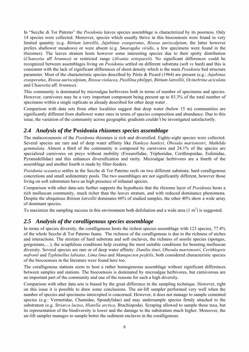
In “Secche di Tor Paterno” the Posidonia leaves species assemblage is characterized by its poorness. Only 14 species were collected. Moreover, species which usually thrive in this biocoenosis were found in very limited quantity (e.g. Bittium latreillii, Jujubinus exasperatus, Rissoa auriscalpium, the latter however prefers shallower meadows) or were absent (e.g. Smaragdia viridis, a few specimens were found in the rhizomes). The leaves stratum hosts however some interesting species due to their spotty distribution (Chauvetia aff brunnea) or restricted range (Alvania settepassii). No significant differences could be recognized between assemblages living on Posidonia settled on different substrata (soft vs hard) and this is consistent with the lack of significant differences of shoot density which is the main Posidonia bed structure parameter. Most of the characteristic species described by Pérès & Picard (1964) are present (e.g.: Jujubinus exasperatus, Rissoa auriscalpium, Rissoa violacea, Pusillina philippi, Bittium latreillii, Ocinebrina aciculata and Chauvetia aff. brunnea). This community is dominated by microalgae herbivores both in terms of number of specimens and species. However, carnivores may be a very important component being present up to 83.3% of the total number of specimens within a single replicate as already described for other deep water . Comparison with data sets from other localities suggest that deep water (below 15 m) communities are significantly different from shallower water ones in terms of species composition and abundance. Due to this issue, the variation of the community across geographic gradients couldn’t be investigated satisfactorily.

2.4 Analysis of the Posidonia rhizomes species assemblage The malacocoenosis of the Posidonia rhizomes is rich and diversified. Eighty-eight species were collected. Several species are rare and of deep water affinity like Hanleya hanleyi, Obesula marisnostri, Mathilda gemmulata. Almost a third of the community is composed by carnivores and 24.1% of the species are specialized carnivores on preys without mobility (Fissurellidae, Triphoridae, Cerithiopsidae, Eulimidae, Pyramidellidae) and this enhances diversification and rarity. Microalgae herbivores are a fourth of the assemblage and another fourth is made by filter-feeders. Posidonia oceanica settles in the Secche di Tor Paterno reefs on two different substrata: hard coralligenous concretions and small sedimentary pools. The two assemblages are not significantly different, however those living on soft substratum have an high presence of infaunal species. Comparison with other data-sets further supports the hypothesis that the rhizome layer of Posidonia hosts a rich molluscan community, much richer than the leaves stratum, and with reduced dominance phenomena. Despite the ubiquitous Bittium latreillii dominates 60% of studied samples, the other 40% show a wide array of dominant species. To maximize the sampling success in this environment both defoliation and a wide area (1 m2) is suggested.

2.5 Analysis of the coralligenous species assemblage In terms of species diversity, the coralligenous hosts the richest species assemblage with 123 species, 77.4% of the whole Secche di Tor Paterno fauna. The richness of the coralligenous is due to the richness of niches and interactions. The mixture of hard substrata and soft enclaves, the richness of sessile species (sponges, gorgonians,…), the sciaphilous conditions help creating the most suitable conditions for boosting molluscan diversity. Several species are rare or of deep water affinity: Danilia tinei, Obesula marisnostri, Cerithiopsis nofronii and Typhinellus labiatus. Lima lima and Manupecten pesfelis, both considered characteristic species of the biocoenosis in the literature were found here too. The coralligenous stations seem to host a rather homogeneous assemblage without significant differences between samples and stations. The biocoenosis is dominated by microalgae herbivores, but carnivorous are an important part of the community and one of the reasons for such a high diversity. Comparison with other data sets is biased by the great difference in the sampling technique. However, right on this issue it is possible to draw some conclusions. The air-lift sampler performed very well when the number of species and specimens intercepted is concerned. However, it does not manage to sample cemented species (e.g.: Vermetidae, Chamidae, Spondylidae) and may undersample species firmly attached to the substratum (e.g. Striarca lactea, Hiatella arctica, Brachiopoda). Scraping allowed to sample these taxa, but its representation of the biodiversity is lower and the damage to the substratum much higher. Moreover, the air-lift sampler manages to sample better the sediment enclaves in the coralligenous.

7

2.6 Analysis of the detritic species assemblage Detritic pools within the reefs may be ascribed to the coastal detritic biocoenosis (DC; Pérès & Picard, 1964). The detritic pools host a poor species assemblage, 22 species, however most of them are exclusive of these soft substrata and these samples have added several species to the knowledge of the malacofauna of the reefs. The only typical molluscan species cited by Pérès & Picard (1964) for this biocoenosis and sampled in the Secche di Tor Paterno pools is Crassopleura maravignae. Specialized carnivores contribute to the biodiversity with a high number of species, up to 40%. Remarkably, bivalves and filter feeders are not dominant despite soft substrata are usually a suitable environment for them. The comparison with data sets from the soft substrata around the reefs and within the boundaries of the Marine Protected Area show that the two assemblages are remarkably different. However, when the analysis is run to understand differences between biocoenoses, the coastal detritic station sampled by Università Tor Vergata is the only without statistically significant differences from the detritic pools confirming the hypothesis that this peculiar environments belong to this biocoenosis, despite it probably represents a different and still to be described facies.

2.7 Agreement between death and living assemblages The analysis of the agreement between death and living assemblages is of interest both in paleoecological reconstruction and in biodiversity conservation, since it could allow the assessment of the biodiversity of an area with a reduced effort and with the advantage of analyzing a time-averaged assemblage which sums up the contribution of several seasons and years. The study has been carried out by a qualitative comparison of samples from the death and living assemblages, with standard metrics and multivariate techniques. The minimum volume for a meaningful analysis has been evaluated in 1 liter of sediment. The analysis was carried out both with the complete data set and with a reduced one with only those species which contribute more than 1% to the overall abundance. The comparison between living and death assemblages showed that there is a high representativeness of sediments in respect of nearby biocoenoses as a result of low bottom transport. It is important to specify that the spatial scale is in the meters or a few tens of meters. This is supported by:

‐ the neat differentiation of the death assemblages nearby different biocoenoses both by a taxonomic and quali-quantitative point of view, despite being spatially close to other biocoenoses

‐ the taxonomic composition of sediments which is strongly influenced by the living communities (e.g. reduced presence of species of the coralligenous endobenthos in the Posidonia assemblage)

‐ The decrease in the values of some fidelity metrics if the full biocoenoses data set is considered instead of only data from the stations nearest to the sediment collection sites

Sediments contain some allochthonous species which thrive in the soft substrata around the reefs (mainly bivalves) and some species which couldn’t be intercepted in the biocoenoses survey due to the little destructive sampling techniques used (e.g. endobenthos species, cementing species). When evaluating the biodiversity of the area, the former should be put apart while the latter are an important addition to the knowledge of the area. Fidelity metrics suggest a good agreement between the living and death assemblages when species richness and taxonomic composition are considered. However, metrics values have to be evaluated in the context of highly diverse molluscan assemblages with little dominance phenomena quite different from those proper of soft substrata which were studied in a number of cases in literature and also different from the few hard substratum cases in literature which focus on a small number of species due to the choice to select only species above 1 or 2 cm in size. The study suggests that fidelity is lower when considering the species dominance where important differences are described between the living and death assemblages. These differences could be associated to the trophism of species and possibly to the species life span.

8

The interpretation of recent and fossil thanatocoenoses is seriously affected by the lack of appropriate knowledge on molluscs life histories. Detailed in formation on diets, seasonality, pluriennial variability of populations and information on life spans of species are keys for a full comprehension of biocoenoses dynamics and their contribution to death assemblages. Reversely, fossil death assemblages need this information for their interpretation in a paleoecological perspective. The study results will help in a better interpretation of paleontological data and foresee good potentialities for the monitoring of biocoenoses using nearby death assemblages. When the latter is considered, the limited diving bottom time required to sample sediments in respect to biocoenoses and the limited field time for treating samples after collection and before laboratory would allow faster surveys and/or greater spatial resolution of sampling. Moreover, the time-averaging effect allows a better description of the fauna, which can be surrogated only by multi-season, pluriennal biocoenoses surveys. However, dead specimens tend to loose important diagnostic characters and may require more skilled personnel for sorting and identification. Another evident drawback of this technique is the limitation to taxa leaving post-mortem remains. Mollusca, however, is the most diverse benthic phylum and therefore allows a good description of the biocoenoses.

9

3 Introduction

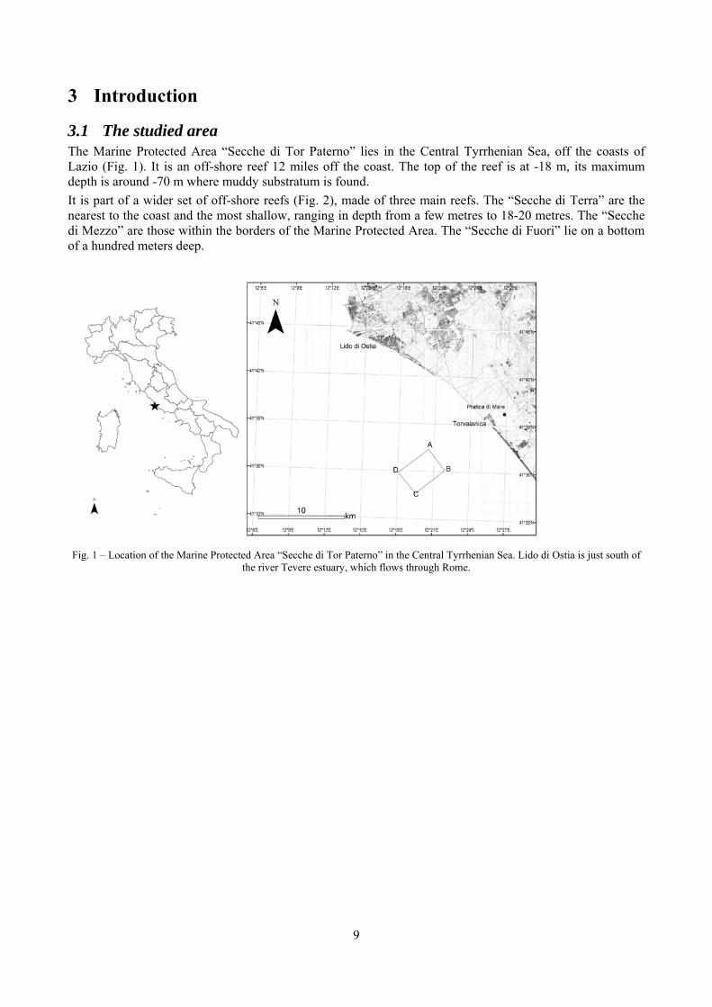
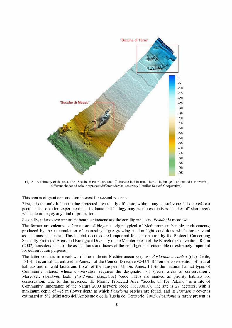
3.1 The studied area The Marine Protected Area “Secche di Tor Paterno” lies in the Central Tyrrhenian Sea, off the coasts of Lazio (Fig. 1). It is an off-shore reef 12 miles off the coast. The top of the reef is at -18 m, its maximum depth is around -70 m where muddy substratum is found. It is part of a wider set of off-shore reefs (Fig. 2), made of three main reefs. The “Secche di Terra” are the nearest to the coast and the most shallow, ranging in depth from a few metres to 18-20 metres. The “Secche di Mezzo” are those within the borders of the Marine Protected Area. The “Secche di Fuori” lie on a bottom of a hundred meters deep.

Fig. 1 – Location of the Marine Protected Area “Secche di Tor Paterno” in the Central Tyrrhenian Sea. Lido di Ostia is just south of

the river Tevere estuary, which flows through Rome.

10

Fig. 2 – Bathimetry of the area. The “Secche di Fuori” are too off-shore to be illustrated here. The image is orientated northwards,

different shades of colour represent different depths. (courtesy Nautilus Società Cooperativa)

This area is of great conservation interest for several reasons. First, it is the only Italian marine protected area totally off-shore, without any coastal zone. It is therefore a peculiar conservation experiment and its fauna and biology may be representatives of other off-shore reefs which do not enjoy any kind of protection. Secondly, it hosts two important benthic biocoenoses: the coralligenous and Posidonia meadows. The former are calcareous formations of biogenic origin typical of Mediterranean benthic environments, produced by the accumulation of encrusting algae growing in dim light conditions which host several associations and facies. This habitat is considered important for conservation by the Protocol Concerning Specially Protected Areas and Biological Diversity in the Mediterranean of the Barcelona Convention. Relini (2002) considers most of the associations and facies of the coralligenous remarkable or extremely important for conservation purposes. The latter consists in meadows of the endemic Mediterranean seagrass Posidonia oceanica ((L.) Delile, 1813). It is an habitat enlisted in Annex I of the Council Directive 92/43/EEC “on the conservation of natural habitats and of wild fauna and flora” of the European Union. Annex I lists the “natural habitat types of Community interest whose conservation requires the designation of special areas of conservation”. Moreover, Posidonia beds (Posidonion oceanicae) (code 1120) are marked as priority habitats for conservation. Due to this presence, the Marine Protected Area “Secche di Tor Paterno” is a site of Community importance of the Natura 2000 network (code IT6000010). The site is 27 hectares, with a maximum depth of –25 m (lower depth at which Posidonia patches are found) and its Posidonia cover is extimated at 5% (Ministero dell'Ambiente e della Tutela del Territorio, 2002). Posidonia is rarely present as

11

a meadow sensu stricto: it is more often present as patches in the coralligenous substratum. Small meadows are present where a large enough sedimentary area is present.

3.2 Why sampling in a marine protected area? Reasons for such a work in a marine protected area lies in the field of conservation, ecology and biodiversity. I stronlgy agree with Giangrande’s view (2003) that inventories of the biodiversity of protected areas are essential. They allow the production of taxonomic lists for the characterization of the different biotopes inside the area and the production of a data set for future comparison. Giangrande discusses this topic about areas proposed for protection, but it applies to already established protected areas too if the basic information is lacking. The main objective of this work was exactly to be a starting point for the study of the biodiversity of the “Secche di Tor Paterno” Marine Protected Area. Despite it is mostly limited to molluscs, its level of detail is far above previous studies. Not only faunistic lists are provided, but different biotopes are characterized and studied on their own and some ecological issues are treated too. The results of this work will be useful for the management of the area especially if further study will be funded in order to have a comparable set of data in a few years. A marine protected area is expected to protect a pristine habitat. Off-shore reefs are a common feature of the Italian coast-line and the results of the analysis of Tor Paterno reefs can be a bench-mark for the analysis of further reefs elsewhere in Italy and in the whole Mediterranean Sea. Last, monitoring of European Union priority habitats like the Posidonia fields is required by law and this can be a contribution towards the fulfillment of these duties.

3.3 The molluscan fauna This study has been focused on the phylum Mollusca. Mollusca is one of the most diverse marine phyla. The number of estimated described marine species is roughly 53,000 with a yearly increment of 350 new species (Bouchet, 2006). The Mediterranean Sea alone hosts almost 2,000 species (Chiarelli in his 1999 annotated check-list recorded 1,792 species, new species have been described and new lessepsian migrants and aliens have been reported since then). The Mediterranean fauna is one of the best known in the world since it has been studied since the 19th century by many scholars. Despite difficult groups still exist and the taxonomy is often complicated by a pletora of unclear taxa and poor comparison with paleontological material, we can assess that most species can be identified to the genus level and a very good percentage to the species level. Molluscs are recognized as excellent descriptors of benthic biocoenoses (Gambi et al., 1982). Moreover they are worldwide recognized as good descriptors of biodiversity (Wells 1998; Mikkelsen & Cracraft 2001; Gladstone 2002; Smith 2005). Most molluscs have a calcareous shell which does not easily dissolve after the death of the animal. Therefore, shells represent an important part of thanatocoenoses and the study of recent biocoenoses allows comparisons with recent and fossil thanatocoenoses. Most Molluscs retain in the adult shell the larval one, allowing inference about the their type of development (planktotrophic vs non-planktotrophic). This has important consequences on the study of the dispersal of species, colonization phenomena and biogeography. The malacofauna of the Secche di Tor Paterno was poorly studied in the past. The most relevant study was carried out by the La Sapienza University in Rome in early ‘90s (1993). The study was aimed at describing the environmental characteristics and fishery resources of the area and covers different biocoenoses and animal and vegetal groups. Molluscs are covered in good detail and a check-list of 445 species is provided. This list is the result of several years of study by University scholars and other researchers from all biocoenoses of the area: from shallow water (a few meters deep) “Secche di Terra” to the deep water (more than a hundred meters) “Secche di Fuori”. The material which allowed to compile this list was obtained in several ways from fishermen’s nets to divers’ samplings, from thanatocoenoses analysis to net sampling on Posidonia leaves. This check-list reports many species from these shallow and deep water environments which nowadays are not within the Marine Protected Area. This study has also been based on benthic samplings by brushing hard substrata on 20×20 centimeters squares from 21 to 37 meters deep,

12

collecting 449 specimens and 40 species. This technical report is poorly known and had little distribution while its synthesis was published a few years later (Ardizzone et al., 1998). The University Tor Vergata in Rome carried out two surveys of the area (Ministero dell’Ambiente, 1998; Cataudella, 2005). Both these surveys have a wider environmental point of view and information on molluscs is limited to the most common species. However, data on coralligenous and Posidonia meadows are given and help to have a better view of these habitats in this area. A few publications have taxonomical interest. In 1984 Amati & Nofroni described a new species of gastropod from the Secche di Tor Paterno (locus typicus): Alvania settepassii (Gastropoda, Rissoidae). In 1987 Amati described two new species from the Mediterranean Sea: Cerithiopsis nofronii (Gastropoda, Cerithiopsidae) and Chrysallida moolenbeeki (Gastropoda, Pyramidellidae). Both these species have a wider Tyrrhenian Sea distribution, however paratypes were selected from the Secche di Tor Paterno. Smaller contributions were made by Oliverio & Villa (1981, 1983). These two papers do not deal specifically with the fauna of the Secche di Tor Paterno, but with the fishermen’s nets samples from boats harboured in Fiumicino (Rome). However, vessels from this town went to the Secche di Tor Paterno area so can indirectly give information on the fauna, especially of the deeper water soft substrata around the rocky reefs. Last, Nicolay & Angioy (1993) illustrate a couple of gastropods: Clathromangelia quadrillum (Gastropoda, Conidae) and Typhinellus sowerbyi (Gastropoda, Muricidae). Despite these are well known Mediterranean species, this paper is one of the very few which illustrates specimens from the area. Despite the survey by La Sapienza University yelds a lot of information and a rich check-list is provided, the malacofauna of the protected area has never been studied in the detail presented here. As better described in chapter 4, most samplings have been made by SCUBA diving with efficient techniques. The huge number of living specimens found has allowed to have a clearer idea of the living malacofauna in the protected reefs and to analyse in detail many local ecological issues. Moreover, the great amount of data allowed to draw general conclusions on the ecology of these biocoenoses. The samplings were so effective that many other phyla were sampled. Research is going on and Brachiopoda has been studied in detail (Evangelisti et al., in print). Brachiopoda were not treated in any other study on this area.

3.4 Abbreviations In graphs and tables the sampled biocoenoses are often indicated by the following abbreviations: COR: coralligenous; FOP: foliar layer of Posidonia oceanica; RIP: rhizome layer of Posidonia oceanica; DET: detritic substratum.

13

4 Materials and methods

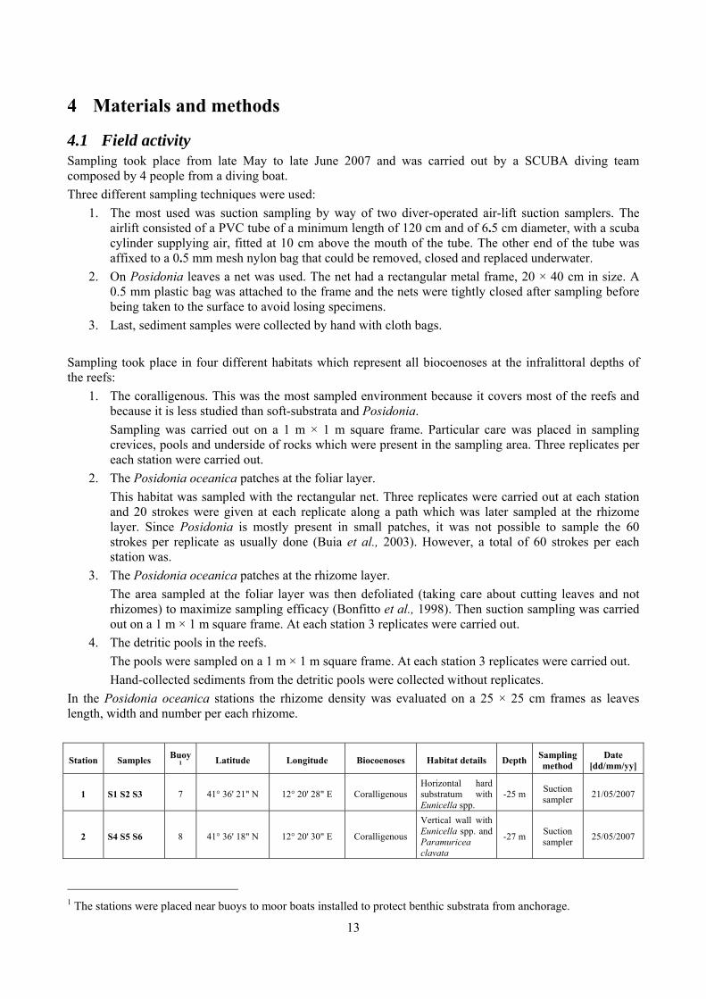
4.1 Field activity Sampling took place from late May to late June 2007 and was carried out by a SCUBA diving team composed by 4 people from a diving boat. Three different sampling techniques were used:

1. The most used was suction sampling by way of two diver-operated air-lift suction samplers. The airlift consisted of a PVC tube of a minimum length of 120 cm and of 6.5 cm diameter, with a scuba cylinder supplying air, fitted at 10 cm above the mouth of the tube. The other end of the tube was affixed to a 0.5 mm mesh nylon bag that could be removed, closed and replaced underwater.

2. On Posidonia leaves a net was used. The net had a rectangular metal frame, 20 × 40 cm in size. A 0.5 mm plastic bag was attached to the frame and the nets were tightly closed after sampling before being taken to the surface to avoid losing specimens.

3. Last, sediment samples were collected by hand with cloth bags. Sampling took place in four different habitats which represent all biocoenoses at the infralittoral depths of the reefs:

1. The coralligenous. This was the most sampled environment because it covers most of the reefs and because it is less studied than soft-substrata and Posidonia. Sampling was carried out on a 1 m × 1 m square frame. Particular care was placed in sampling crevices, pools and underside of rocks which were present in the sampling area. Three replicates per each station were carried out.

2. The Posidonia oceanica patches at the foliar layer. This habitat was sampled with the rectangular net. Three replicates were carried out at each station and 20 strokes were given at each replicate along a path which was later sampled at the rhizome layer. Since Posidonia is mostly present in small patches, it was not possible to sample the 60 strokes per replicate as usually done (Buia et al., 2003). However, a total of 60 strokes per each station was.

3. The Posidonia oceanica patches at the rhizome layer. The area sampled at the foliar layer was then defoliated (taking care about cutting leaves and not rhizomes) to maximize sampling efficacy (Bonfitto et al., 1998). Then suction sampling was carried out on a 1 m × 1 m square frame. At each station 3 replicates were carried out.

4. The detritic pools in the reefs. The pools were sampled on a 1 m × 1 m square frame. At each station 3 replicates were carried out. Hand-collected sediments from the detritic pools were collected without replicates.

In the Posidonia oceanica stations the rhizome density was evaluated on a 25 × 25 cm frames as leaves length, width and number per each rhizome.

Station Samples Buoy1 Latitude Longitude Biocoenoses Habitat details Depth Sampling

method Date

[dd/mm/yy]

1 S1 S2 S3 7 41° 36' 21" N 12° 20' 28" E Coralligenous Horizontal hard substratum with Eunicella spp.

-25 m Suction sampler 21/05/2007

2 S4 S5 S6 8 41° 36' 18" N 12° 20' 30" E Coralligenous

Vertical wall with Eunicella spp. and Paramuricea clavata

-27 m Suction sampler 25/05/2007

1 The stations were placed near buoys to moor boats installed to protect benthic substrata from anchorage.

14

Station Samples Buoy1 Latitude Longitude Biocoenoses Habitat details Depth Sampling

method Date

[dd/mm/yy]

3 S7 S8 S9 8 41° 36' 18" N 12° 20' 30" E Coralligenous Horizontal hard substratum with Eunicella spp.

-25 m Suction sampler 25/05/2007

4 S10 S11 S12 6 41° 36' 15" N 12° 20' 29" E Coralligenous Horizontal hard substratum with Eunicella spp.

-26 m Suction sampler 07/06/2007

5 S13 S14 S15 6 41° 36' 15" N 12° 20' 29" E Detritic Detritic pools in coralligenous substratum

-28 m Suction sampler 07/06/2007

10 S16 S17 S22 1 41° 36' 13" N 12° 20' 30" E Coralligenous Horizontal hard substratum with rare Eunicella spp.

-20 m Suction sampler 20/06/2007

11 S182 S19 S20 S21 4 41° 36' 07" N 12° 20' 20" E Coralligenous

Horizontal hard substratum with Eunicella spp.

-25 m Suction sampler 21/06/2007

- R1 R2 R33 1 41° 36' 13" N 12° 20' 30" E Posidonia oceanica

Posidonia patches on hard substratum – foliar layer

-24m Net 21/05/2007

6 R4 R5 R6 7 41° 36' 21" N 12° 20' 28" E Posidonia oceanica

Posidonia patches on hard substratum – foliar layer

-26 m Net 08/06/2007

8 R7 R8 R9 1 41° 36' 13" N 12° 20' 30" E Posidonia oceanica

Posidonia field on soft substratum – foliar layer

-26 m Net 20/06/2007

7 SP1 SP2 SP3 7 41° 36' 21" N 12° 20' 28" E Posidonia oceanica

Posidonia patches on hard substratum – rhizome layer

-26 m Suction sampler 08/06/2007

9 SP4 SP5 SP6 1 41° 36' 13" N 12° 20' 30" E Posidonia oceanica

Posidonia field on soft substratum – rhizome layer

-26 m Suction sampler 20/06/2007

- D1 Substratum sediment

1 41° 36' 13" N 12° 20' 30" E Posidonia oceanica

Thanatocoenoses nearby small Posidonia meadow

-25 m Hand collected 20/06/2007

- D2 Substratum sediment

8 41° 36' 18" N 12° 20' 30" E Coralligenous

Thanatocoenoses at the base of a wall with Eunicella spp. and Paramuricea clavata

-27m Hand collected 25/05/2007

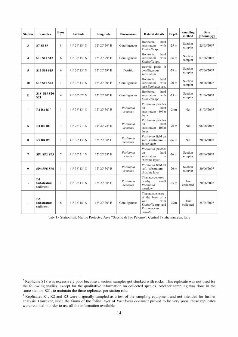
Tab. 1 - Station list, Marine Protected Area “Secche di Tor Paterno”, Central Tyrrhenian Sea, Italy

2 Replicate S18 was excessively poor because a suction sampler got stucked with rocks. This replicate was not used for the following studies, except for the qualitative information on collected species. Another sampling was done in the same station, S21, to maintain the three replicates per station rule. 3 Replicates R1, R2 and R3 were originally sampled as a test of the sampling equipment and not intended for further analysis. However, since the fauna of the foliar layer of Posidonia oceanica proved to be very poor, these replicates were retained in order to use all the information available.

15

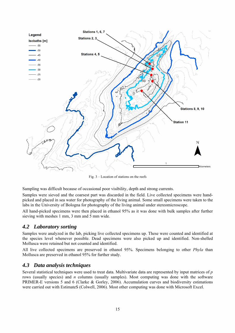
Fig. 3 – Location of stations on the reefs

Sampling was difficult because of occasional poor visibility, depth and strong currents. Samples were sieved and the coarsest part was discarded in the field. Live collected specimens were hand-picked and placed in sea water for photography of the living animal. Some small specimens were taken to the labs in the University of Bologna for photography of the living animal under stereomicroscope. All hand-picked specimens were then placed in ethanol 95% as it was done with bulk samples after further sieving with meshes 1 mm, 3 mm and 5 mm wide.

4.2 Laboratory sorting Samples were analyzed in the lab, picking live collected specimens up. These were counted and identified at the species level whenever possible. Dead specimens were also picked up and identified. Non-shelled Mollusca were retained but not counted and identified. All live collected specimens are preserved in ethanol 95%. Specimens belonging to other Phyla than Mollusca are preserved in ethanol 95% for further study.

4.3 Data analysis techniques Several statistical techniques were used to treat data. Multivariate data are represented by input matrices of p rows (usually species) and n columns (usually samples). Most computing was done with the software PRIMER-E versions 5 and 6 (Clarke & Gorley, 2006). Accumulation curves and biodiversity estimations were carried out with EstimateS (Colwell, 2006). Most other computing was done with Microsoft Excel.

16

The description below is taken from a few statistical manuals (e.g.: Clarke & Warwick, 2001; Soliani, 2005) and has the aim to shortly describe the data analysis techniques. A short comment about the technique results or parameters choices is usually included so that choices in the analysis can be fully understood.

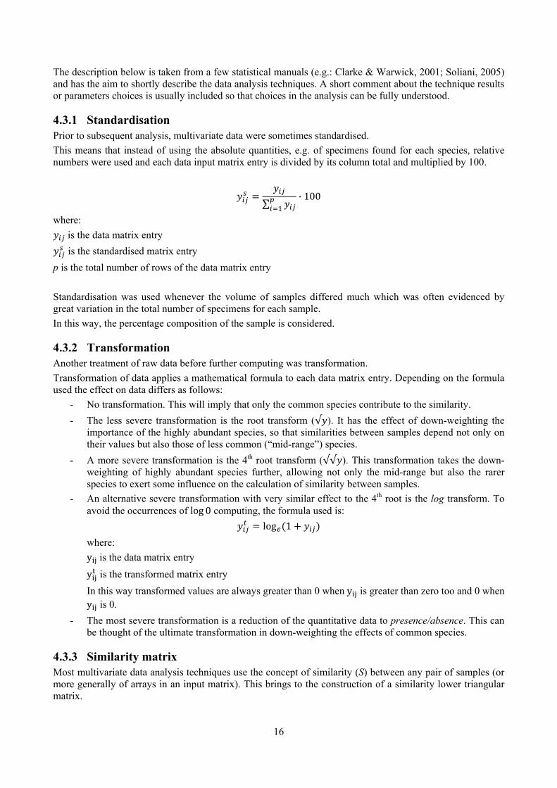
4.3.1 Standardisation Prior to subsequent analysis, multivariate data were sometimes standardised. This means that instead of using the absolute quantities, e.g. of specimens found for each species, relative numbers were used and each data input matrix entry is divided by its column total and multiplied by 100.

∑· 100

where: is the data matrix entry is the standardised matrix entry

p is the total number of rows of the data matrix entry Standardisation was used whenever the volume of samples differed much which was often evidenced by great variation in the total number of specimens for each sample. In this way, the percentage composition of the sample is considered.

4.3.2 Transformation Another treatment of raw data before further computing was transformation. Transformation of data applies a mathematical formula to each data matrix entry. Depending on the formula used the effect on data differs as follows:

- No transformation. This will imply that only the common species contribute to the similarity. - The less severe transformation is the root transform (√ ). It has the effect of down-weighting the

importance of the highly abundant species, so that similarities between samples depend not only on their values but also those of less common (“mid-range”) species.

- A more severe transformation is the 4th root transform (√√ ). This transformation takes the down-weighting of highly abundant species further, allowing not only the mid-range but also the rarer species to exert some influence on the calculation of similarity between samples.

- An alternative severe transformation with very similar effect to the 4th root is the log transform. To avoid the occurrences of log 0 computing, the formula used is:

log 1 where: y is the data matrix entry y is the transformed matrix entry In this way transformed values are always greater than 0 when y is greater than zero too and 0 when y is 0.

- The most severe transformation is a reduction of the quantitative data to presence/absence. This can be thought of the ultimate transformation in down-weighting the effects of common species.

4.3.3 Similarity matrix Most multivariate data analysis techniques use the concept of similarity (S) between any pair of samples (or more generally of arrays in an input matrix). This brings to the construction of a similarity lower triangular matrix.

17

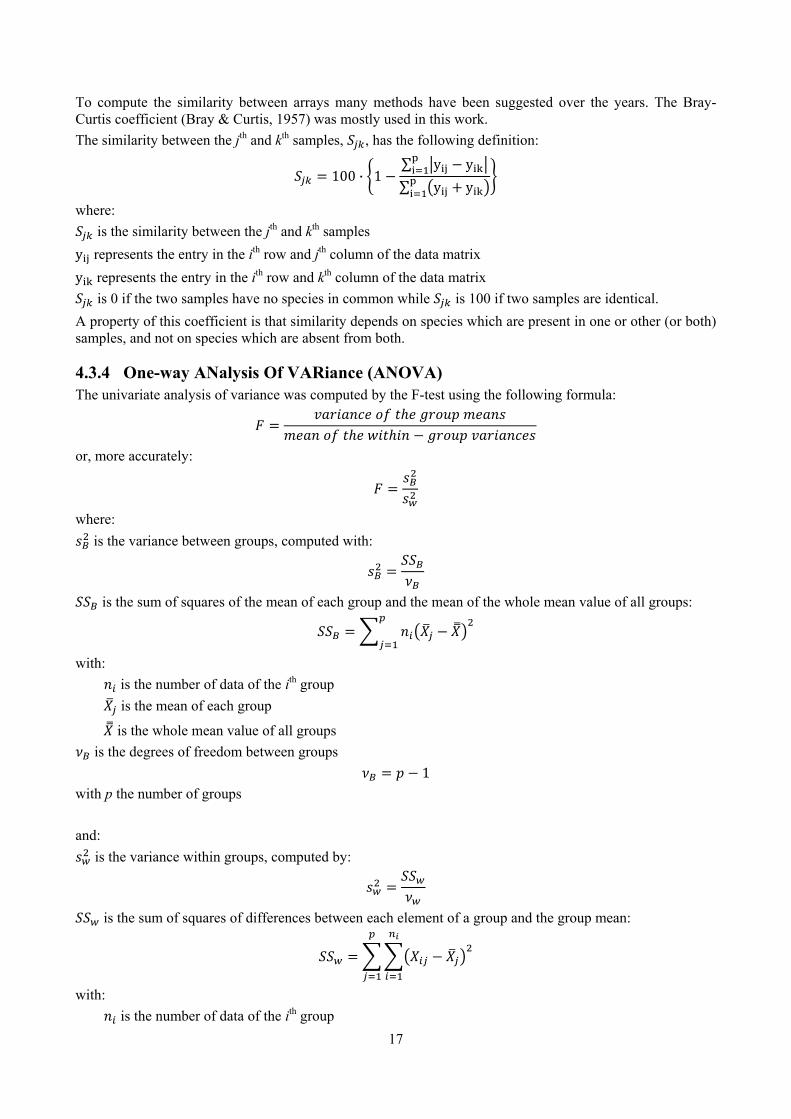
To compute the similarity between arrays many methods have been suggested over the years. The Bray-Curtis coefficient (Bray & Curtis, 1957) was mostly used in this work. The similarity between the jth and kth samples, , has the following definition:

100 · 1∑ y y∑ y y

where: is the similarity between the jth and kth samples

y represents the entry in the ith row and jth column of the data matrix y represents the entry in the ith row and kth column of the data matrix

is 0 if the two samples have no species in common while is 100 if two samples are identical. A property of this coefficient is that similarity depends on species which are present in one or other (or both) samples, and not on species which are absent from both.

4.3.4 One-way ANalysis Of VARiance (ANOVA) The univariate analysis of variance was computed by the F-test using the following formula:

or, more accurately:

where: is the variance between groups, computed with:

is the sum of squares of the mean of each group and the mean of the whole mean value of all groups:

with: is the number of data of the ith group is the mean of each group

is the whole mean value of all groups is the degrees of freedom between groups

1 with p the number of groups and:

is the variance within groups, computed by:

is the sum of squares of differences between each element of a group and the group mean:

with: is the number of data of the ith group

18

is the element of the group is the mean of each group

is the degrees of freedom between groups

with n the total number of elements of all groups and p the number of groups. Statistical significance is tested for by comparing the F test statistic to the F-distribution. The null hypothesis is rejected when the test statistic is greater than the tabled value. Significance level was usually fixed at α=0.05. The F-test can be used as a global test and as a pairwise test between the different types of samples. However, in this case the risk of type I errors (detecting a difference when it does not exist) will cumulate. Therefore the Bonferroni correction may be applied and the significance level is reduced to

where n is the number of pairwise comparisons, despite the increase of risk of type II errors (not detecting a difference when one exists). Please note that the meaning of indices (i, j) and other simbols (n, p, etc) used here is different from those used when treating data matrices for multivariate analysis.

4.3.5 Mann–Whitney U test The Mann–Whitney U test is a non-parametric test for assessing whether two independent samples of observations come from the same distribution. It is virtually identical to performing an ordinary parametric two-sample t-test on the data after ranking over the combined samples. This test has been used every time the hypothesis of normality needed for a t-test was not supported.

4.3.6 Cluster analysis Cluster analysis aims to find natural groupings of samples such that samples within a group are more similar to each other, generally, than samples in different groups. It may be useful to see whether replicate samples within a site form a cluster that is distinct from replicates within other sites and can be an overview of differences between type of sites. It is a method that can be used in cases where the samples are expected to divide into well-defined groups, while it is not appropriate when samples are expected to respond to a more continuous gradient of variation. The clustering technique used here is the hierarchical agglomerative method which takes the similarity matrix as its starting point and successively fuse the samples into groups and the groups into larger clusters creating a dendrogram. The process involves the iterative construction of similarity matrices by successive fusing of samples. The combination of similarity values may follow three methods:

- Single linkage, - Complete linkage, - Group-average link.

Single link clustering has a tendency to produce chains of linked samples, with each successive stage just adding another single sample onto a large group. Complete linkage will tend to have the opposite effect, with an emphasis on small clusters at the early stages. Group-average link tends to stay in the middle between these two extremes.

19

4.3.7 Non-metric Multi-Dimensional Scaling (MDS) This is an ordination procedure first introduced by Shepard (1962) and Kruskal (1964). It constructs a map of the samples in a specified number of dimensions. Its starting point is a similarity or dissimilarity matrix. Its interpretation is in terms of the relative values of similarity to each other and the ranks of the similarities are the only information used by a successful non-metric MDS ordination. However, there will be some distortion between the similarity rankings and the corresponding distance rankings in the ordination plot and the degree of this distortion is called stress. Stress can be thought of the as measuring the difficulty involved in compressing the sample relationships into (usually) two dimensions. Stress values can be evaluated in this way:

- Stress <0.05 gives an excellent representation; - Stress <0.1 corresponds to a good ordination; - Stress <0.2 still gives a potentially useful 2-dimensional picture; - Stress >0.3 indicates that the points are close to being arbitraly placed in the 2-dimensional

ordination space. To ascertain whether the final result is reliable, the procedure is repeated several times from a different starting point. If the same (lowest stress) solution re-appears from a number of different starts then there is a strong assurance, though never a total guarantee, that this is indeed the best solution. So the number of restarts is a measure of the strength of the final plot.

4.3.8 Multivariate ANalysis Of SIMilarities (ANOSIM) ANOSIM is a simple non-parametric permutation procedure applied to the similarity matrix underlying the ordination of samples. It tests whether there are statistically significant differences among different multi-variate samples. It was described by Clarke et al (1988). The starting point of its procedure is computing a test statistic reflecting the observed differences between sites contrasted with differences among replicates within sites. The test is based on the rank similarities between samples in the underlying triangular similarity matrix. The test statistic R is computed by:

12

where: is the average of rank similarities arising from all pairs of replicates between different sites is the average of rank similarities among replicates within sites

and 1

2

with n the total number of samples under consideration. R has the following properties:

- It belongs to the range (-1,1) and usually fall between 0 and 1; - It is equal to 1 only if all replicates within sites are more similar to each other than any replicates

from different sites; - It is approximately zero if the null hypothesis is true, so that similarities between and within sites

will be the same on average (differences are due to casuality and not to sites properties); - It is below zero when similarities across different sites are higher than those within sites and it is

highly unlikely. The second step of the procedure is recomputing the statistic under permutations. If the null hypothesis is true that there are no differences across sites, then there will be little effect on the value of R if the labels identifying which replicates belong to which sites are arbitraly rearranged. Since the number of possible

20

permutations grows quickly with the increase in the number of samples, the full set of permutations is randomly sampled (usually with replacement) to give the null distribution of R. The last step of the procedure is to calculate the significance level by referring the observed R value to its permutation distribution. If the null hypothesis is true, the likely spread of values of R is given by the random rearrangements, so that if the true value of R looks unlikely to have come from this distribution there is evidence to reject the null hypothesis. The level of significance can be computed by:

11

where: t is the number of simulated R values as large or greater than the observed R; T is the total number of simulated values. It is therefore important to highlight that the interpretation of the value of R is strongly related to its distribution and that the possibility of having a significant permutation depends on the number of replicates which has not to be too low.

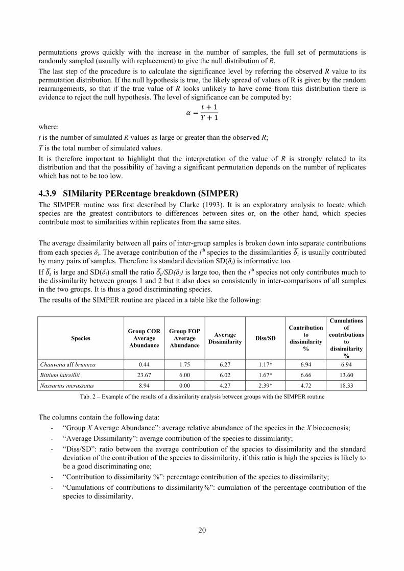
4.3.9 SIMilarity PERcentage breakdown (SIMPER) The SIMPER routine was first described by Clarke (1993). It is an exploratory analysis to locate which species are the greatest contributors to differences between sites or, on the other hand, which species contribute most to similarities within replicates from the same sites. The average dissimilarity between all pairs of inter-group samples is broken down into separate contributions from each species δi. The average contribution of the ith species to the dissimilarities is usually contributed by many pairs of samples. Therefore its standard deviation SD(δi) is informative too. If is large and SD(δi) small the ratio /SD(δi) is large too, then the ith species not only contributes much to the dissimilarity between groups 1 and 2 but it also does so consistently in inter-comparisons of all samples in the two groups. It is thus a good discriminating species. The results of the SIMPER routine are placed in a table like the following:

Species Group COR

Average Abundance

Group FOP Average

Abundance

Average Dissimilarity Diss/SD

Contribution to

dissimilarity %

Cumulations of

contributions to

dissimilarity%

Chauvetia aff brunnea 0.44 1.75 6.27 1.17* 6.94 6.94

Bittium latreillii 23.67 6.00 6.02 1.67* 6.66 13.60

Nassarius incrassatus 8.94 0.00 4.27 2.39* 4.72 18.33

Tab. 2 – Example of the results of a dissimilarity analysis between groups with the SIMPER routine

The columns contain the following data:

- “Group X Average Abundance”: average relative abundance of the species in the X biocoenosis; - “Average Dissimilarity”: average contribution of the species to dissimilarity; - “Diss/SD”: ratio between the average contribution of the species to dissimilarity and the standard

deviation of the contribution of the species to dissimilarity, if this ratio is high the species is likely to be a good discriminating one;

- “Contribution to dissimilarity %”: percentage contribution of the species to dissimilarity; - “Cumulations of contributions to dissimilarity%”: cumulation of the percentage contribution of the

species to dissimilarity.

21

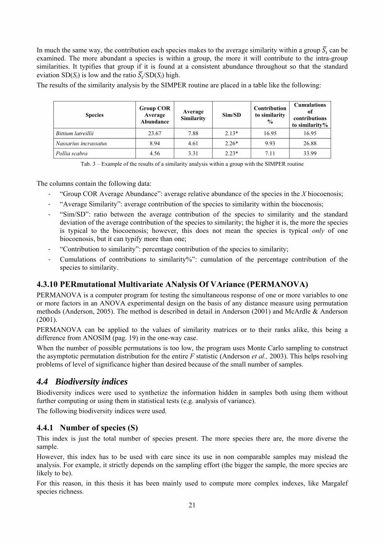
In much the same way, the contribution each species makes to the average similarity within a group can be examined. The more abundant a species is within a group, the more it will contribute to the intra-group similarities. It typifies that group if it is found at a consistent abundance throughout so that the standard eviation SD(Si) is low and the ratio /SD(Si) high. The results of the similarity analysis by the SIMPER routine are placed in a table like the following:

Species Group COR

Average Abundance

Average Similarity Sim/SD

Contribution to similarity

%

Cumulations of

contributions to similarity%

Bittium latreillii 23.67 7.88 2.13* 16.95 16.95

Nassarius incrassatus 8.94 4.61 2.26* 9.93 26.88

Pollia scabra 4.56 3.31 2.23* 7.11 33.99

Tab. 3 – Example of the results of a similarity analysis within a group with the SIMPER routine

The columns contain the following data:

‐ “Group COR Average Abundance”: average relative abundance of the species in the X biocoenosis; ‐ “Average Similarity”: average contribution of the species to similarity within the biocenosis; ‐ “Sim/SD”: ratio between the average contribution of the species to similarity and the standard

deviation of the average contribution of the species to similarity; the higher it is, the more the species is typical to the biocoenosis; however, this does not mean the species is typical only of one biocoenosis, but it can typify more than one;

‐ “Contribution to similarity”: percentage contribution of the species to similarity; ‐ Cumulations of contributions to similarity%”: cumulation of the percentage contribution of the

species to similarity.

4.3.10 PERmutational Multivariate ANalysis Of VAriance (PERMANOVA) PERMANOVA is a computer program for testing the simultaneous response of one or more variables to one or more factors in an ANOVA experimental design on the basis of any distance measure using permutation methods (Anderson, 2005). The method is described in detail in Anderson (2001) and McArdle & Anderson (2001). PERMANOVA can be applied to the values of similarity matrices or to their ranks alike, this being a difference from ANOSIM (pag. 19) in the one-way case. When the number of possible permutations is too low, the program uses Monte Carlo sampling to construct the asymptotic permutation distribution for the entire F statistic (Anderson et al., 2003). This helps resolving problems of level of significance higher than desired because of the small number of samples.

4.4 Biodiversity indices Biodiversity indices were used to synthetize the information hidden in samples both using them without further computing or using them in statistical tests (e.g. analysis of variance). The following biodiversity indices were used.

4.4.1 Number of species (S) This index is just the total number of species present. The more species there are, the more diverse the sample. However, this index has to be used with care since its use in non comparable samples may mislead the analysis. For example, it strictly depends on the sampling effort (the bigger the sample, the more species are likely to be). For this reason, in this thesis it has been mainly used to compute more complex indexes, like Margalef species richness.

22

4.4.2 Number of specimens (N) This index is not a true diversity index, but it is an abundance index. It gives information on the quantity of specimens per sample and when used in relation to the area sampled can describe the density of living specimens in the different samples.

4.4.3 Margalef’s species richness (d) Since the number of species is sample dependent, it is not suitable when different sampling techniques are used or when there are doubts that sampling has been carried out with the same efficacy. Margalef’s species richness index is based on the number of species, but incorporates the total number of individuals too:

1log

Where: S is the number of species; N is the number of specimens.

4.4.4 Shannon index (H’) This is the most commonly used diversity index and is computed by:

· log

where: is the proportion of the total count arising from the ith species:

The higher the value of the index, the more diverse is the sample. Note that the natural logarithm is used. The Shannon index can be sensitive to the degree of sampling effort and should be compared across equivalent sampling desings.

4.4.5 Equitability (J’) This index expresses how evenly the individuals are distributed among the different species. It is referred as Pielou’s evenness index too. It is computed by:

log

This index is close to 1 when all species are equally abundant. It is close to 0 when the sample is highly dominated by a few species.

4.4.6 Simpson index (λ) This is another commonly used index which has a number of forms. Here two forms are used:

1 1

where: is the proportion of the total count arising from the ith species:

23

The index λ has a natural interpretation as the probability that any two individuals from the sample, chosen at random, are from the same species. λ is always ≤1. It is a dominance index, in the sense that its largest values correspond to assemblages whose total abundance is dominated by one, or a very few, of the species present. Its complement 1- λ is thus an equitability or evennes index, taking its largest value when all species have the same abundance.

4.5 Biodiversity estimators Accumulation curves were drawn with EstimateS 8 (Colwell, 2006) with 50 randomizations. Biodiversity estimations were done using the Bootstrap non-parametric first order estimator (Smith et al., 1984) and the Jackknife non-parametric second order estimator (Burnham et al., 1979). The first order estimators take into consideration singletons only, while the second order estimators take into consideration doubletons too. Singletons are defined by Novotny & Basset (2000) as species represented by a single specimen in the sample. Doubletons are those represented by two specimens in the sample. Species found as a single individual in component communities are called “local singletons”, those found as a single individual in the combined data set are called “unique singletons”.

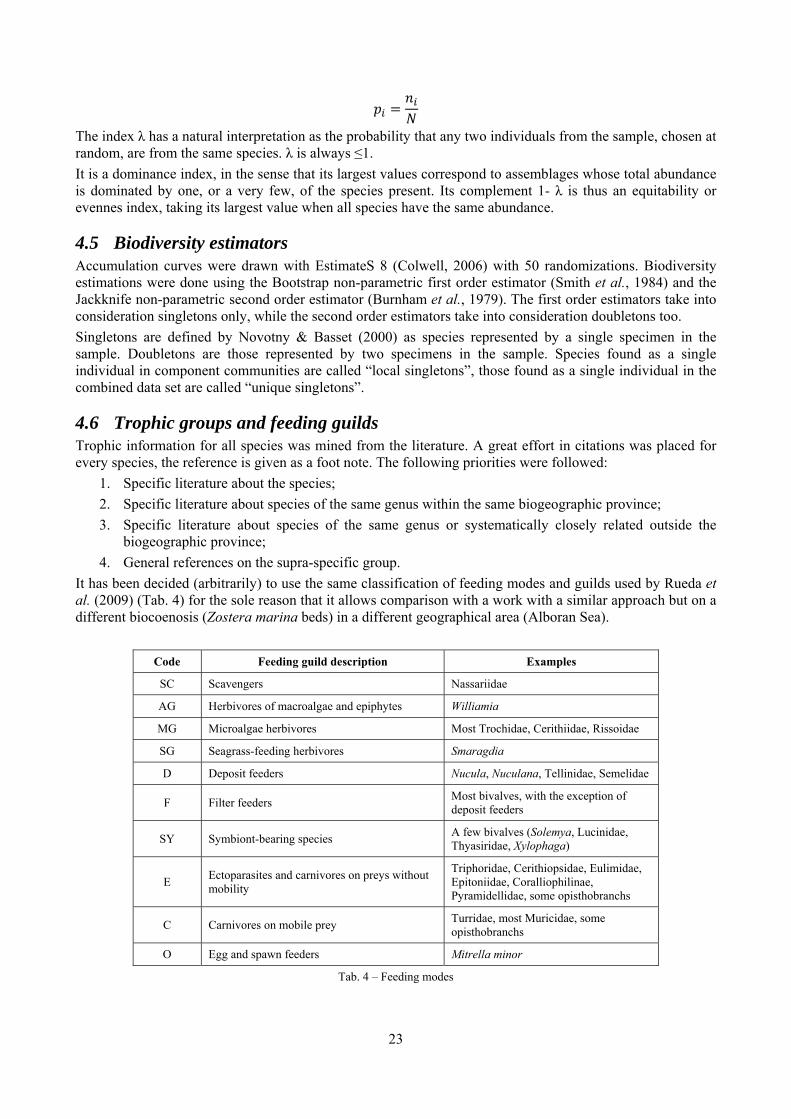
4.6 Trophic groups and feeding guilds Trophic information for all species was mined from the literature. A great effort in citations was placed for every species, the reference is given as a foot note. The following priorities were followed:

1. Specific literature about the species; 2. Specific literature about species of the same genus within the same biogeographic province; 3. Specific literature about species of the same genus or systematically closely related outside the

biogeographic province; 4. General references on the supra-specific group.

It has been decided (arbitrarily) to use the same classification of feeding modes and guilds used by Rueda et al. (2009) (Tab. 4) for the sole reason that it allows comparison with a work with a similar approach but on a different biocoenosis (Zostera marina beds) in a different geographical area (Alboran Sea).

Code Feeding guild description Examples

SC Scavengers Nassariidae

AG Herbivores of macroalgae and epiphytes Williamia

MG Microalgae herbivores Most Trochidae, Cerithiidae, Rissoidae

SG Seagrass-feeding herbivores Smaragdia

D Deposit feeders Nucula, Nuculana, Tellinidae, Semelidae

F Filter feeders Most bivalves, with the exception of deposit feeders

SY Symbiont-bearing species A few bivalves (Solemya, Lucinidae, Thyasiridae, Xylophaga)

E Ectoparasites and carnivores on preys without mobility

Triphoridae, Cerithiopsidae, Eulimidae, Epitoniidae, Coralliophilinae, Pyramidellidae, some opisthobranchs

C Carnivores on mobile prey Turridae, most Muricidae, some opisthobranchs

O Egg and spawn feeders Mitrella minor

Tab. 4 – Feeding modes

24

4.7 The role of species in describing biocoenoses When describing the fauna of biocoenoses, species can be ascribed to three different categories:

‐ Characteristic species: these species are typical of a biocenosis, meaning that they are usually found in it notwithstanding their abundance which can be high (constant species) or low (sporadical species). This group can be divided in two further groups: the exclusive species which can be found only in a given biotope or the species which prefer the biocoenosis, meaning that in that biotope they are significantly more abundant than in others.

‐ Accompanying species: these species are normally present in the given biocoenosis as in others. These species may appear at the given depth level, or can be indicators of edaphic conditions or may have wide ecological tolerance and are usually ubiquitarian.

‐ Accidental species: these are species characteristic of other biocoenoses but occasionally found in the given biotope where they experience limited success (reduced life span, increased predation, inability to reproduce,…).

Particular attention should be given in classifying species which are parasites, symbiontic, commensals or are species-specific epibiontic. Their attitude towards biocoenoses will depend by their host and not by themselves, of course. Another issue to be considered in general, but which is probably of low interest in benthic molluscs, is that some species may have a different affiliation to biocoenoses in different stages of their development.

25

5 Sampling results and efficacy Two main sampling techniques were used in this survey: the hand-net on Posidonia leaves and a suction air-lift sampler on other biocoenoses. Both of them were used by SCUBA divers. The use of hand-nets on Posidonia leaves is a technique described in several studies and recently standardised (Buia et al., 2003): sixty strokes per replicate are required. However, this method is thought for ‘true’ Posidonia fields, while in the Tor Paterno reefs we had to face small patches of Posidonia or very scattered fields because plants grow on hard coralligenous substratum. For this reason we had to use only 20 strokes per replicate, however taking care of making three replicates per station to have the 60 strokes for each station for being able to compare data with those collected by other scholars. This is a semi-quantitative technique. On the other hand, the sampling technique for the rhizomes, the coralligenous and the detritic pools is less standardised. The vagile fauna of the rhizomes of Posidonia is sampled in many ways (Buia et al., 2003), but the most efficient and least destructive is the diver-operated suction sampler. It is a quantitative technique. However, there is not a standardisation of this method. One square meter sampled areas are reported in literature (Russo et al., 1986; Giangrande, 1985) too as 40 centimeter squares (Buia et al., 2003). When it comes to the coralligenous, direct sampling techniques for hard substrata are usually brushing and air-lift suction sampling (Bianchi et al., 2003). Since the investigated area is protected, the suction sampler was preferred because it is less destructive. However, boring endobenthos (e.g. Lithophaga, Gastrochaena) is difficult to obtain in this way and the analysis of thanatocenoses is useful to have a more complete view of the biodiversity of this complex biocoenosis. Boring endobenthos is present in thanatocoenosis due to the periodic erosion of the bioherms. The issue of the mimimum area to sample is not resolved yet (Bianchi et al., 2003). Due to the complex structure of the coralligenous any two-dimensional size does not describe accurately the quantity of “useful surface” for organisms since this environment is rich in crevices, stones and biohermatic species which greatily augment the surface used by animals and molluscs in particular. Soft substrata are usually surveyed by indirect techniques like grabs and dredges (Castelli et al., 2003). However, the soft substrata in the reefs are detritic pools of limited extension. The largest pools may be a few tens of meters wide. It is therefore necessary to use a direct technique. Since the main interest were molluscs which usually are buried in the first centimeters of sediment, the air-lift suction sampler was tested here. No standardisation exists for this particular technique in this environment. A 1 m2 area per replicate was sampled.

5.1 Results Sampling brought 2,495 living specimens of shelled molluscs. The number of species and specimens for each species are summarized in the following tables. Station 1 2 3 4 10 11

Replicate S1 S2 S3 S4 S5 S6 S7 S8 S9 S10 S11 S12 S16 S17 S22 S19 S20 S21

Specimens 173 25 70 90 126 27 119 113 37 126 123 49 159 62 153 118 122 101

Species 53 11 26 33 34 14 40 33 13 29 35 25 43 25 42 39 44 37

Tab. 5 – Quantitative results for the replicates in the coralligenous

Station - 6 8

Replicate R1 R2 R3 R4 R5 R6 R7 R8 R9

Specimens 24 6 25 6 3 19 0 6 5

Species 5 3 5 2 2 7 0 5 3

Tab. 6 – Quantitative results for the replicates in the Posidonia oceanica leaves

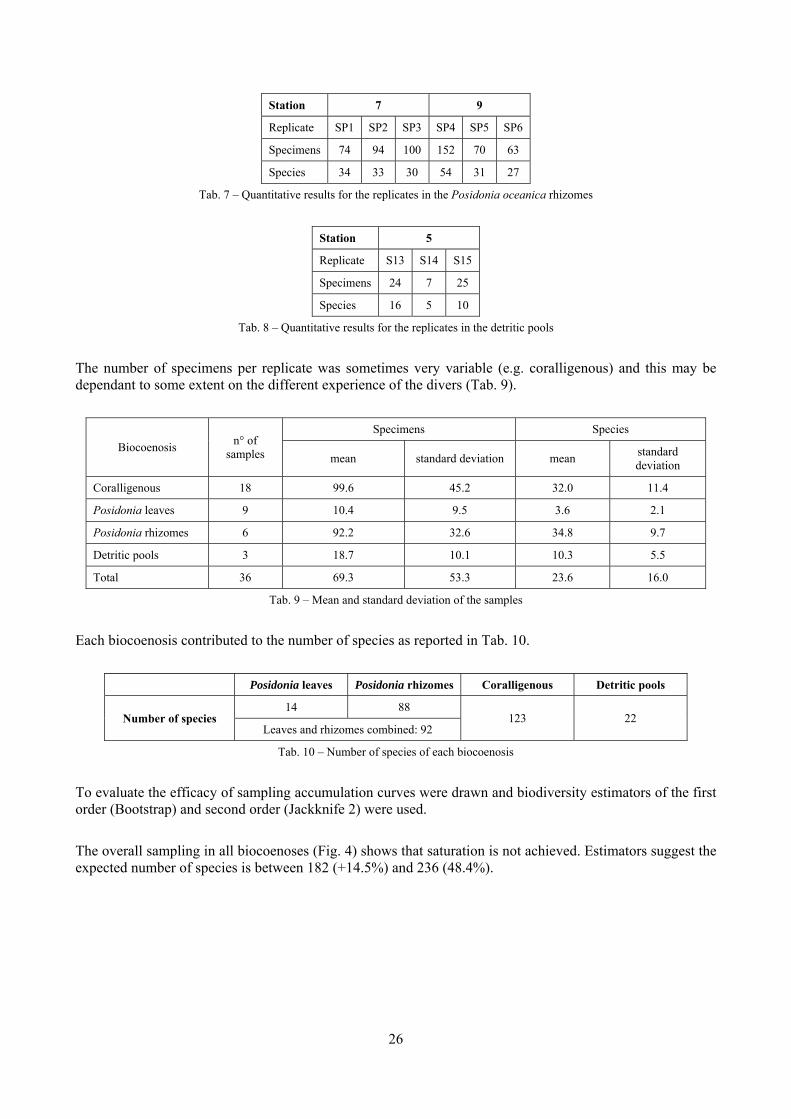
26

Station 7 9

Replicate SP1 SP2 SP3 SP4 SP5 SP6

Specimens 74 94 100 152 70 63

Species 34 33 30 54 31 27

Tab. 7 – Quantitative results for the replicates in the Posidonia oceanica rhizomes

Station 5

Replicate S13 S14 S15

Specimens 24 7 25

Species 16 5 10

Tab. 8 – Quantitative results for the replicates in the detritic pools

The number of specimens per replicate was sometimes very variable (e.g. coralligenous) and this may be dependant to some extent on the different experience of the divers (Tab. 9).

Biocoenosis n° of samples

Specimens Species

mean standard deviation mean standard deviation

Coralligenous 18 99.6 45.2 32.0 11.4

Posidonia leaves 9 10.4 9.5 3.6 2.1

Posidonia rhizomes 6 92.2 32.6 34.8 9.7

Detritic pools 3 18.7 10.1 10.3 5.5

Total 36 69.3 53.3 23.6 16.0

Tab. 9 – Mean and standard deviation of the samples

Each biocoenosis contributed to the number of species as reported in Tab. 10.

Posidonia leaves Posidonia rhizomes Coralligenous Detritic pools

Number of species 14 88

123 22 Leaves and rhizomes combined: 92

Tab. 10 – Number of species of each biocoenosis

To evaluate the efficacy of sampling accumulation curves were drawn and biodiversity estimators of the first order (Bootstrap) and second order (Jackknife 2) were used. The overall sampling in all biocoenoses (Fig. 4) shows that saturation is not achieved. Estimators suggest the expected number of species is between 182 (+14.5%) and 236 (48.4%).

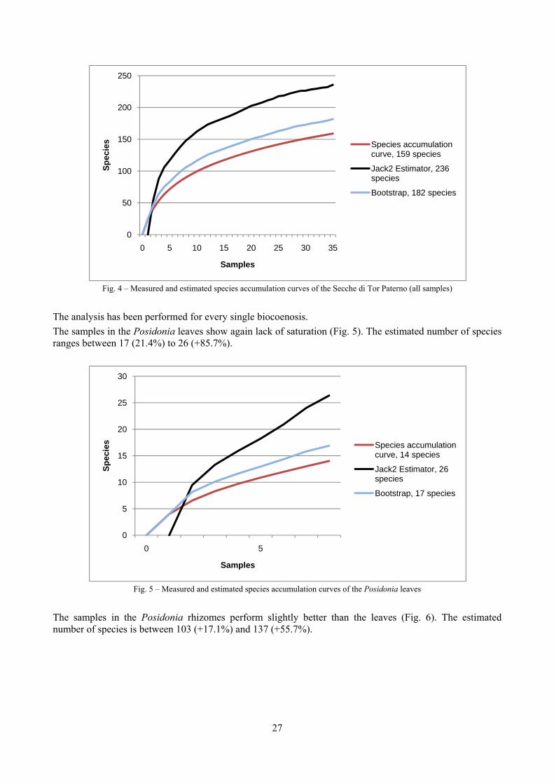
27

Fig. 4 – Measured and estimated species accumulation curves of the Secche di Tor Paterno (all samples)

The analysis has been performed for every single biocoenosis. The samples in the Posidonia leaves show again lack of saturation (Fig. 5). The estimated number of species ranges between 17 (21.4%) to 26 (+85.7%).

Fig. 5 – Measured and estimated species accumulation curves of the Posidonia leaves

The samples in the Posidonia rhizomes perform slightly better than the leaves (Fig. 6). The estimated number of species is between 103 (+17.1%) and 137 (+55.7%).

0

50

100

150

200

250

0 5 10 15 20 25 30 35

Spec

ies

Samples

Species accumulation curve, 159 species

Jack2 Estimator, 236 species

Bootstrap, 182 species

0

5

10

15

20

25

30

0 5

Spec

ies

Samples

Species accumulation curve, 14 species

Jack2 Estimator, 26 species

Bootstrap, 17 species

28

Fig. 6 - Measured and estimated species accumulation curves of the Posidonia rhizomes

The coralligenous showed the best saturation (Fig. 7). The estimated number of species is between 141 (+14.6%) and 186 (+ 51.2%).

Fig. 7 - Measured and estimated species accumulation curves of the coralligenous

The detritic pools did not achieve any saturation (Fig. 8). The estimated number of species spans from 27 (+22.7%) to 36 (+63.6%).

0

30

60

90

120

150

0 5

Spec

ies

Samples

Species accumulation curve, 88 species

Jack2 Estimator, 137 species

Bootstrap, 103 species

0

50

100

150

200

250

0 5 10 15

Spec

ies

Samples

Species accumulation curve, 123 species

Jack2 Estimator, 186 species

Bootstrap, 141 species

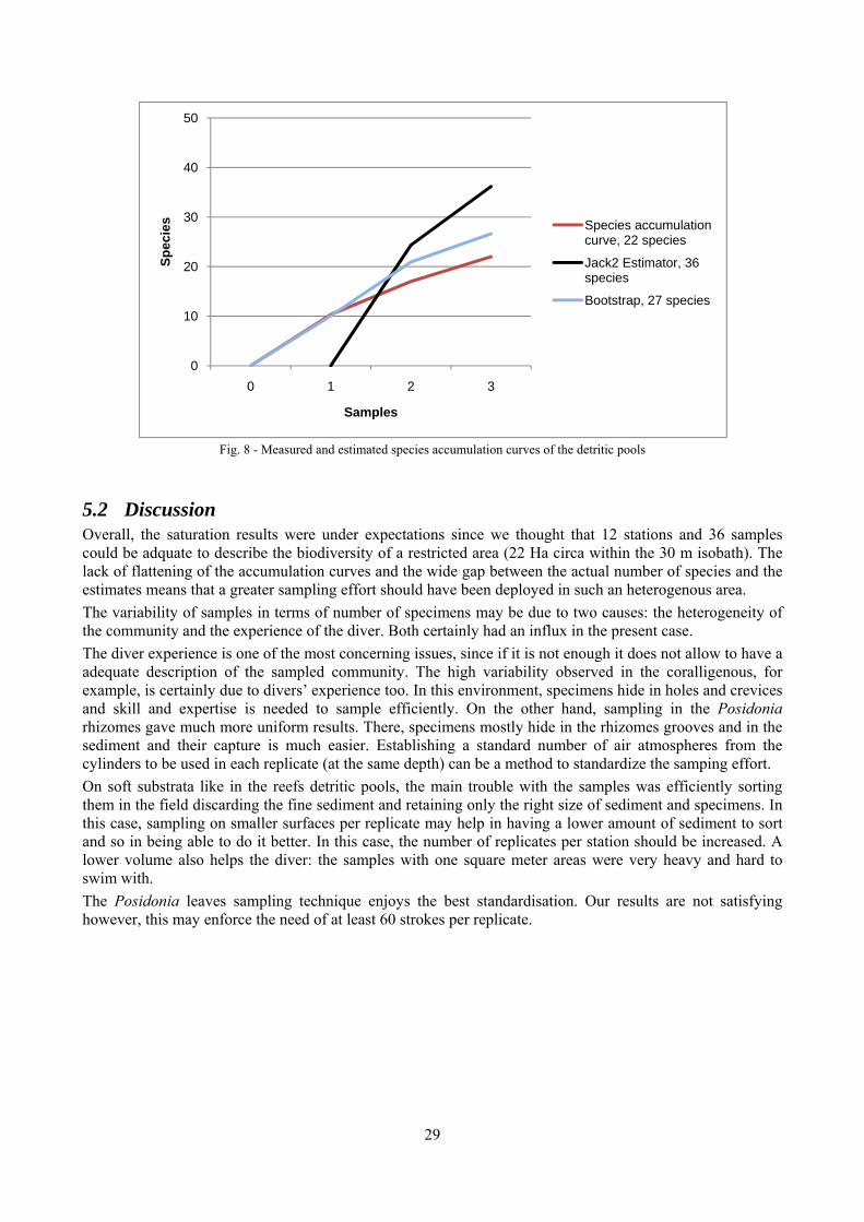
29

Fig. 8 - Measured and estimated species accumulation curves of the detritic pools

5.2 Discussion Overall, the saturation results were under expectations since we thought that 12 stations and 36 samples could be adquate to describe the biodiversity of a restricted area (22 Ha circa within the 30 m isobath). The lack of flattening of the accumulation curves and the wide gap between the actual number of species and the estimates means that a greater sampling effort should have been deployed in such an heterogenous area. The variability of samples in terms of number of specimens may be due to two causes: the heterogeneity of the community and the experience of the diver. Both certainly had an influx in the present case. The diver experience is one of the most concerning issues, since if it is not enough it does not allow to have a adequate description of the sampled community. The high variability observed in the coralligenous, for example, is certainly due to divers’ experience too. In this environment, specimens hide in holes and crevices and skill and expertise is needed to sample efficiently. On the other hand, sampling in the Posidonia rhizomes gave much more uniform results. There, specimens mostly hide in the rhizomes grooves and in the sediment and their capture is much easier. Establishing a standard number of air atmospheres from the cylinders to be used in each replicate (at the same depth) can be a method to standardize the samping effort. On soft substrata like in the reefs detritic pools, the main trouble with the samples was efficiently sorting them in the field discarding the fine sediment and retaining only the right size of sediment and specimens. In this case, sampling on smaller surfaces per replicate may help in having a lower amount of sediment to sort and so in being able to do it better. In this case, the number of replicates per station should be increased. A lower volume also helps the diver: the samples with one square meter areas were very heavy and hard to swim with. The Posidonia leaves sampling technique enjoys the best standardisation. Our results are not satisfying however, this may enforce the need of at least 60 strokes per replicate.

0

10

20

30

40

50

0 1 2 3

Spec

ies

Samples

Species accumulation curve, 22 species

Jack2 Estimator, 36 species

Bootstrap, 27 species

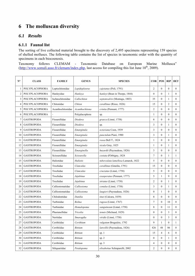
30

6 The molluscan diversity

6.1 Results

6.1.1 Faunal list The sorting of live collected material brought to the discovery of 2,495 specimens representing 159 species of shelled molluscs. The following table contains the list of species in taxonomic order with the quantity of specimens in each biocoenosis. Taxonomy follows CLEMAM - Taxonomic Database on European Marine Mollusca” (http://www.somali.asso.fr/clemam/index.php, last access for compiling this list June 10th, 2009).

N° CLASS FAMILY GENUS SPECIES COR POS RIP DET

1 POLYPLACOPHORA Leptochitonidae Lepidopleurus cajetanus (Poli, 1791) 2 0 0 0

2 POLYPLACOPHORA Hanleyidae Hanleya hanleyi (Bean in Thorpe, 1844) 0 0 1 0

3 POLYPLACOPHORA Ischnochitonidae Callochiton septemvalvis (Montagu, 1803) 35 0 1 0

4 POLYPLACOPHORA Chitonidae Chiton corallinus (Risso, 1826) 15 0 2 0

5 POLYPLACOPHORA Acanthochitonidae Acanthochitona crinita (Pennant, 1777) 2 0 0 0

6 POLYPLACOPHORA - Polyplacophora sp. 1 0 0 0

7 GASTROPODA Fissurellidae Diodora graeca (Linné, 1758) 8 0 0 0

8 GASTROPODA Fissurellidae Diodora sp. 3 0 1 0

9 GASTROPODA Fissurellidae Emarginula octaviana Coen, 1939 3 0 0 0

10 GASTROPODA Fissurellidae Emarginula punctulum Piani, 1980 3 0 1 0

11 GASTROPODA Fissurellidae Emarginula rosea Bell T., 1824 1 0 0 0

12 GASTROPODA Fissurellidae Emarginula sicula Gray, 1825 1 0 1 0

13 GASTROPODA Fissurellidae Emarginella huzardii (Payraudeau, 1826) 3 0 0 0

14 GASTROPODA Scissurellidae Scissurella costata d'Orbigny, 1824 7 0 1 1

15 GASTROPODA Haliotidae Haliotis tuberculata lamellosa Lamarck, 1822 5 0 0 0

16 GASTROPODA Trochidae Clanculus corallinus (Gmelin, 1791) 15 0 0 0

17 GASTROPODA Trochidae Clanculus cruciatus (Linné, 1758) 5 0 0 0

18 GASTROPODA Trochidae Jujubinus exasperatus (Pennant, 1777) 5 1 9 0

19 GASTROPODA Trochidae Jujubinus striatus (Linné, 1758) 2 0 1 0

20 GASTROPODA Calliostomatidae Calliostoma conulus (Linné, 1758) 3 0 1 0

21 GASTROPODA Calliostomatidae Calliostoma laugieri (Payraudeau, 1826) 0 1 0 0

22 GASTROPODA Chilodontidae Danilia tinei (Calcara, 1839) 8 0 0 0

23 GASTROPODA Turbinidae Bolma rugosa (Linné, 1767) 7 0 10 0

24 GASTROPODA Turbinidae Homalopoma sanguineum (Linné, 1758) 8 0 11 0

25 GASTROPODA Phasianellidae Tricolia tenuis (Michaud, 1829) 0 0 3 0

26 GASTROPODA Neritidae Smaragdia viridis (Linné, 1758) 0 0 3 0

27 GASTROPODA Cerithiidae Cerithium vulgatum Bruguière, 1792 9 1 0 1

28 GASTROPODA Cerithiidae Bittium latreillii (Payraudeau, 1826) 426 48 86 0

29 GASTROPODA Cerithiidae Bittium sp. 1 15 4 6 0

30 GASTROPODA Cerithiidae Bittium sp. 2 0 0 1 0

31 GASTROPODA Cerithiidae Bittium sp. 3 4 0 0 0

32 GASTROPODA Siliquariidae Petalopoma elisabettae Schiaparelli, 2002 2 0 0 0

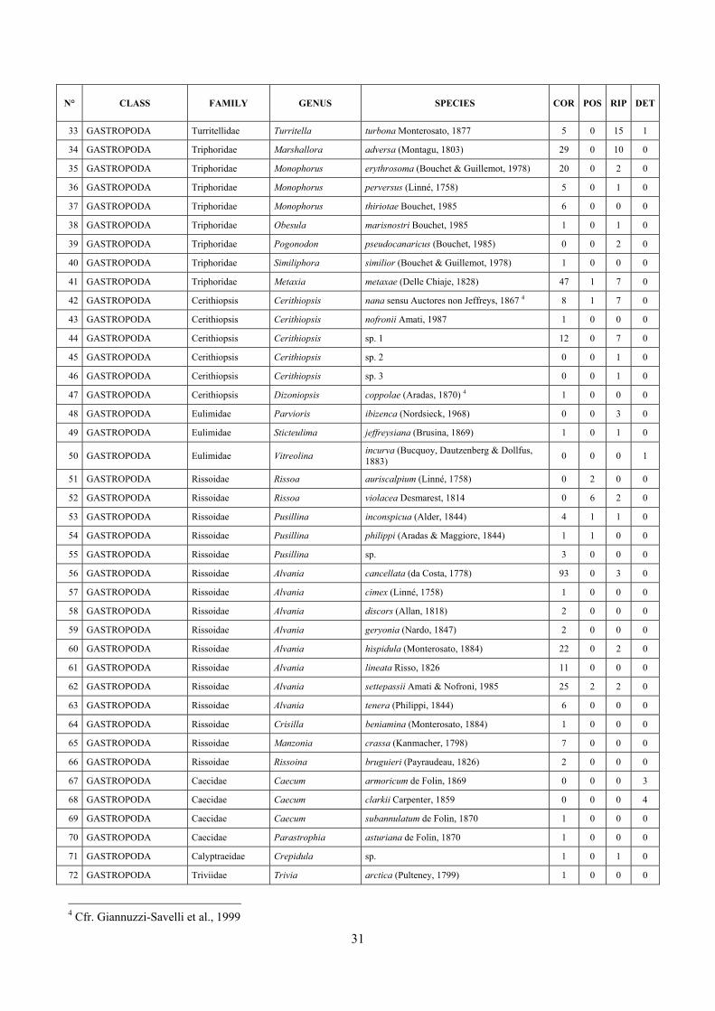
31

N° CLASS FAMILY GENUS SPECIES COR POS RIP DET

33 GASTROPODA Turritellidae Turritella turbona Monterosato, 1877 5 0 15 1

34 GASTROPODA Triphoridae Marshallora adversa (Montagu, 1803) 29 0 10 0

35 GASTROPODA Triphoridae Monophorus erythrosoma (Bouchet & Guillemot, 1978) 20 0 2 0

36 GASTROPODA Triphoridae Monophorus perversus (Linné, 1758) 5 0 1 0

37 GASTROPODA Triphoridae Monophorus thiriotae Bouchet, 1985 6 0 0 0

38 GASTROPODA Triphoridae Obesula marisnostri Bouchet, 1985 1 0 1 0

39 GASTROPODA Triphoridae Pogonodon pseudocanaricus (Bouchet, 1985) 0 0 2 0

40 GASTROPODA Triphoridae Similiphora similior (Bouchet & Guillemot, 1978) 1 0 0 0

41 GASTROPODA Triphoridae Metaxia metaxae (Delle Chiaje, 1828) 47 1 7 0

42 GASTROPODA Cerithiopsis Cerithiopsis nana sensu Auctores non Jeffreys, 1867 4 8 1 7 0

43 GASTROPODA Cerithiopsis Cerithiopsis nofronii Amati, 1987 1 0 0 0

44 GASTROPODA Cerithiopsis Cerithiopsis sp. 1 12 0 7 0

45 GASTROPODA Cerithiopsis Cerithiopsis sp. 2 0 0 1 0

46 GASTROPODA Cerithiopsis Cerithiopsis sp. 3 0 0 1 0

47 GASTROPODA Cerithiopsis Dizoniopsis coppolae (Aradas, 1870) 4 1 0 0 0

48 GASTROPODA Eulimidae Parvioris ibizenca (Nordsieck, 1968) 0 0 3 0

49 GASTROPODA Eulimidae Sticteulima jeffreysiana (Brusina, 1869) 1 0 1 0

50 GASTROPODA Eulimidae Vitreolina incurva (Bucquoy, Dautzenberg & Dollfus, 1883) 0 0 0 1

51 GASTROPODA Rissoidae Rissoa auriscalpium (Linné, 1758) 0 2 0 0

52 GASTROPODA Rissoidae Rissoa violacea Desmarest, 1814 0 6 2 0

53 GASTROPODA Rissoidae Pusillina inconspicua (Alder, 1844) 4 1 1 0

54 GASTROPODA Rissoidae Pusillina philippi (Aradas & Maggiore, 1844) 1 1 0 0

55 GASTROPODA Rissoidae Pusillina sp. 3 0 0 0

56 GASTROPODA Rissoidae Alvania cancellata (da Costa, 1778) 93 0 3 0

57 GASTROPODA Rissoidae Alvania cimex (Linné, 1758) 1 0 0 0

58 GASTROPODA Rissoidae Alvania discors (Allan, 1818) 2 0 0 0

59 GASTROPODA Rissoidae Alvania geryonia (Nardo, 1847) 2 0 0 0

60 GASTROPODA Rissoidae Alvania hispidula (Monterosato, 1884) 22 0 2 0

61 GASTROPODA Rissoidae Alvania lineata Risso, 1826 11 0 0 0

62 GASTROPODA Rissoidae Alvania settepassii Amati & Nofroni, 1985 25 2 2 0

63 GASTROPODA Rissoidae Alvania tenera (Philippi, 1844) 6 0 0 0

64 GASTROPODA Rissoidae Crisilla beniamina (Monterosato, 1884) 1 0 0 0

65 GASTROPODA Rissoidae Manzonia crassa (Kanmacher, 1798) 7 0 0 0

66 GASTROPODA Rissoidae Rissoina bruguieri (Payraudeau, 1826) 2 0 0 0

67 GASTROPODA Caecidae Caecum armoricum de Folin, 1869 0 0 0 3

68 GASTROPODA Caecidae Caecum clarkii Carpenter, 1859 0 0 0 4

69 GASTROPODA Caecidae Caecum subannulatum de Folin, 1870 1 0 0 0

70 GASTROPODA Caecidae Parastrophia asturiana de Folin, 1870 1 0 0 0

71 GASTROPODA Calyptraeidae Crepidula sp. 1 0 1 0

72 GASTROPODA Triviidae Trivia arctica (Pulteney, 1799) 1 0 0 0

4 Cfr. Giannuzzi-Savelli et al., 1999

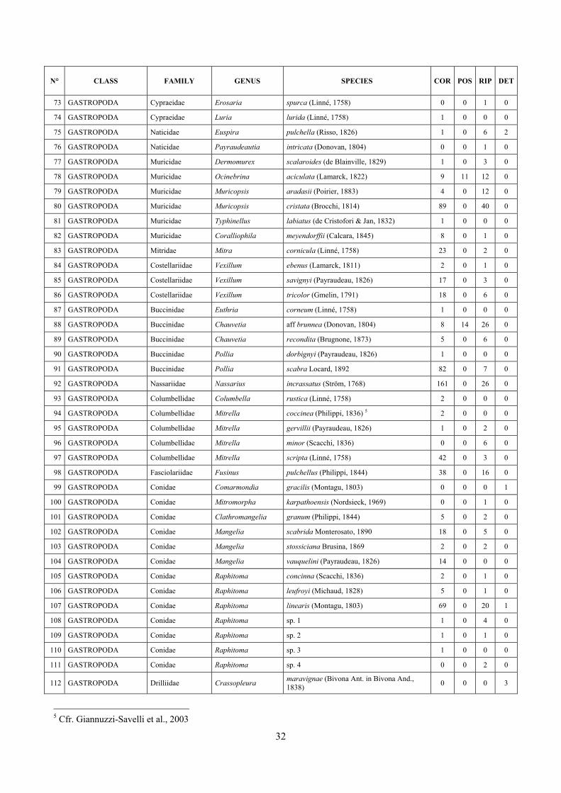
32

N° CLASS FAMILY GENUS SPECIES COR POS RIP DET

73 GASTROPODA Cypraeidae Erosaria spurca (Linné, 1758) 0 0 1 0

74 GASTROPODA Cypraeidae Luria lurida (Linné, 1758) 1 0 0 0

75 GASTROPODA Naticidae Euspira pulchella (Risso, 1826) 1 0 6 2

76 GASTROPODA Naticidae Payraudeautia intricata (Donovan, 1804) 0 0 1 0

77 GASTROPODA Muricidae Dermomurex scalaroides (de Blainville, 1829) 1 0 3 0

78 GASTROPODA Muricidae Ocinebrina aciculata (Lamarck, 1822) 9 11 12 0

79 GASTROPODA Muricidae Muricopsis aradasii (Poirier, 1883) 4 0 12 0

80 GASTROPODA Muricidae Muricopsis cristata (Brocchi, 1814) 89 0 40 0

81 GASTROPODA Muricidae Typhinellus labiatus (de Cristofori & Jan, 1832) 1 0 0 0

82 GASTROPODA Muricidae Coralliophila meyendorffii (Calcara, 1845) 8 0 1 0

83 GASTROPODA Mitridae Mitra cornicula (Linné, 1758) 23 0 2 0

84 GASTROPODA Costellariidae Vexillum ebenus (Lamarck, 1811) 2 0 1 0

85 GASTROPODA Costellariidae Vexillum savignyi (Payraudeau, 1826) 17 0 3 0

86 GASTROPODA Costellariidae Vexillum tricolor (Gmelin, 1791) 18 0 6 0

87 GASTROPODA Buccinidae Euthria corneum (Linné, 1758) 1 0 0 0

88 GASTROPODA Buccinidae Chauvetia aff brunnea (Donovan, 1804) 8 14 26 0

89 GASTROPODA Buccinidae Chauvetia recondita (Brugnone, 1873) 5 0 6 0

90 GASTROPODA Buccinidae Pollia dorbignyi (Payraudeau, 1826) 1 0 0 0

91 GASTROPODA Buccinidae Pollia scabra Locard, 1892 82 0 7 0

92 GASTROPODA Nassariidae Nassarius incrassatus (Ström, 1768) 161 0 26 0

93 GASTROPODA Columbellidae Columbella rustica (Linné, 1758) 2 0 0 0

94 GASTROPODA Columbellidae Mitrella coccinea (Philippi, 1836) 5 2 0 0 0

95 GASTROPODA Columbellidae Mitrella gervillii (Payraudeau, 1826) 1 0 2 0

96 GASTROPODA Columbellidae Mitrella minor (Scacchi, 1836) 0 0 6 0

97 GASTROPODA Columbellidae Mitrella scripta (Linné, 1758) 42 0 3 0

98 GASTROPODA Fasciolariidae Fusinus pulchellus (Philippi, 1844) 38 0 16 0

99 GASTROPODA Conidae Comarmondia gracilis (Montagu, 1803) 0 0 0 1

100 GASTROPODA Conidae Mitromorpha karpathoensis (Nordsieck, 1969) 0 0 1 0

101 GASTROPODA Conidae Clathromangelia granum (Philippi, 1844) 5 0 2 0

102 GASTROPODA Conidae Mangelia scabrida Monterosato, 1890 18 0 5 0

103 GASTROPODA Conidae Mangelia stossiciana Brusina, 1869 2 0 2 0

104 GASTROPODA Conidae Mangelia vauquelini (Payraudeau, 1826) 14 0 0 0

105 GASTROPODA Conidae Raphitoma concinna (Scacchi, 1836) 2 0 1 0

106 GASTROPODA Conidae Raphitoma leufroyi (Michaud, 1828) 5 0 1 0

107 GASTROPODA Conidae Raphitoma linearis (Montagu, 1803) 69 0 20 1

108 GASTROPODA Conidae Raphitoma sp. 1 1 0 4 0

109 GASTROPODA Conidae Raphitoma sp. 2 1 0 1 0

110 GASTROPODA Conidae Raphitoma sp. 3 1 0 0 0

111 GASTROPODA Conidae Raphitoma sp. 4 0 0 2 0

112 GASTROPODA Drilliidae Crassopleura maravignae (Bivona Ant. in Bivona And., 1838) 0 0 0 3

5 Cfr. Giannuzzi-Savelli et al., 2003

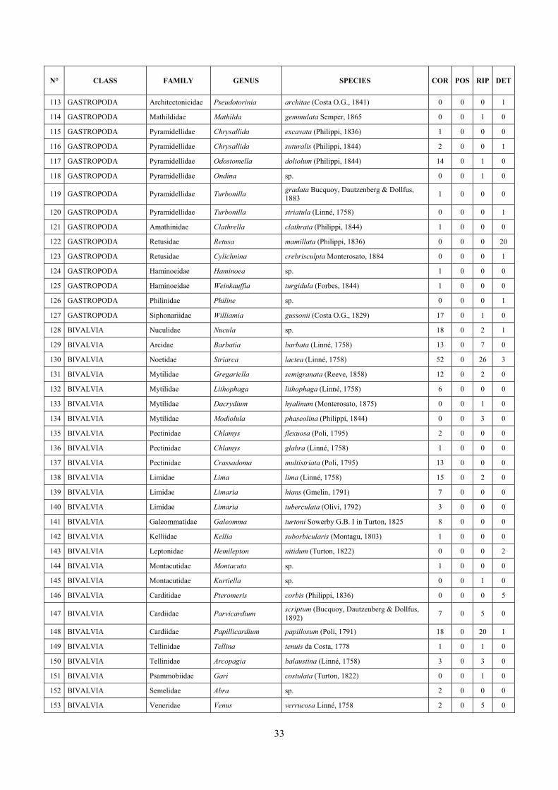
33

N° CLASS FAMILY GENUS SPECIES COR POS RIP DET

113 GASTROPODA Architectonicidae Pseudotorinia architae (Costa O.G., 1841) 0 0 0 1

114 GASTROPODA Mathildidae Mathilda gemmulata Semper, 1865 0 0 1 0

115 GASTROPODA Pyramidellidae Chrysallida excavata (Philippi, 1836) 1 0 0 0

116 GASTROPODA Pyramidellidae Chrysallida suturalis (Philippi, 1844) 2 0 0 1

117 GASTROPODA Pyramidellidae Odostomella doliolum (Philippi, 1844) 14 0 1 0

118 GASTROPODA Pyramidellidae Ondina sp. 0 0 1 0

119 GASTROPODA Pyramidellidae Turbonilla gradata Bucquoy, Dautzenberg & Dollfus, 1883 1 0 0 0

120 GASTROPODA Pyramidellidae Turbonilla striatula (Linné, 1758) 0 0 0 1

121 GASTROPODA Amathinidae Clathrella clathrata (Philippi, 1844) 1 0 0 0

122 GASTROPODA Retusidae Retusa mamillata (Philippi, 1836) 0 0 0 20

123 GASTROPODA Retusidae Cylichnina crebrisculpta Monterosato, 1884 0 0 0 1

124 GASTROPODA Haminoeidae Haminoea sp. 1 0 0 0

125 GASTROPODA Haminoeidae Weinkauffia turgidula (Forbes, 1844) 1 0 0 0

126 GASTROPODA Philinidae Philine sp. 0 0 0 1

127 GASTROPODA Siphonariidae Williamia gussonii (Costa O.G., 1829) 17 0 1 0

128 BIVALVIA Nuculidae Nucula sp. 18 0 2 1

129 BIVALVIA Arcidae Barbatia barbata (Linné, 1758) 13 0 7 0

130 BIVALVIA Noetidae Striarca lactea (Linné, 1758) 52 0 26 3

131 BIVALVIA Mytilidae Gregariella semigranata (Reeve, 1858) 12 0 2 0

132 BIVALVIA Mytilidae Lithophaga lithophaga (Linné, 1758) 6 0 0 0

133 BIVALVIA Mytilidae Dacrydium hyalinum (Monterosato, 1875) 0 0 1 0

134 BIVALVIA Mytilidae Modiolula phaseolina (Philippi, 1844) 0 0 3 0

135 BIVALVIA Pectinidae Chlamys flexuosa (Poli, 1795) 2 0 0 0

136 BIVALVIA Pectinidae Chlamys glabra (Linné, 1758) 1 0 0 0

137 BIVALVIA Pectinidae Crassadoma multistriata (Poli, 1795) 13 0 0 0

138 BIVALVIA Limidae Lima lima (Linné, 1758) 15 0 2 0

139 BIVALVIA Limidae Limaria hians (Gmelin, 1791) 7 0 0 0

140 BIVALVIA Limidae Limaria tuberculata (Olivi, 1792) 3 0 0 0

141 BIVALVIA Galeommatidae Galeomma turtoni Sowerby G.B. I in Turton, 1825 8 0 0 0

142 BIVALVIA Kelliidae Kellia suborbicularis (Montagu, 1803) 1 0 0 0

143 BIVALVIA Leptonidae Hemilepton nitidum (Turton, 1822) 0 0 0 2

144 BIVALVIA Montacutidae Montacuta sp. 1 0 0 0

145 BIVALVIA Montacutidae Kurtiella sp. 0 0 1 0

146 BIVALVIA Carditidae Pteromeris corbis (Philippi, 1836) 0 0 0 5

147 BIVALVIA Cardiidae Parvicardium scriptum (Bucquoy, Dautzenberg & Dollfus, 1892) 7 0 5 0

148 BIVALVIA Cardiidae Papillicardium papillosum (Poli, 1791) 18 0 20 1

149 BIVALVIA Tellinidae Tellina tenuis da Costa, 1778 1 0 1 0

150 BIVALVIA Tellinidae Arcopagia balaustina (Linné, 1758) 3 0 3 0

151 BIVALVIA Psammobiidae Gari costulata (Turton, 1822) 0 0 1 0

152 BIVALVIA Semelidae Abra sp. 2 0 0 0

153 BIVALVIA Veneridae Venus verrucosa Linné, 1758 2 0 5 0

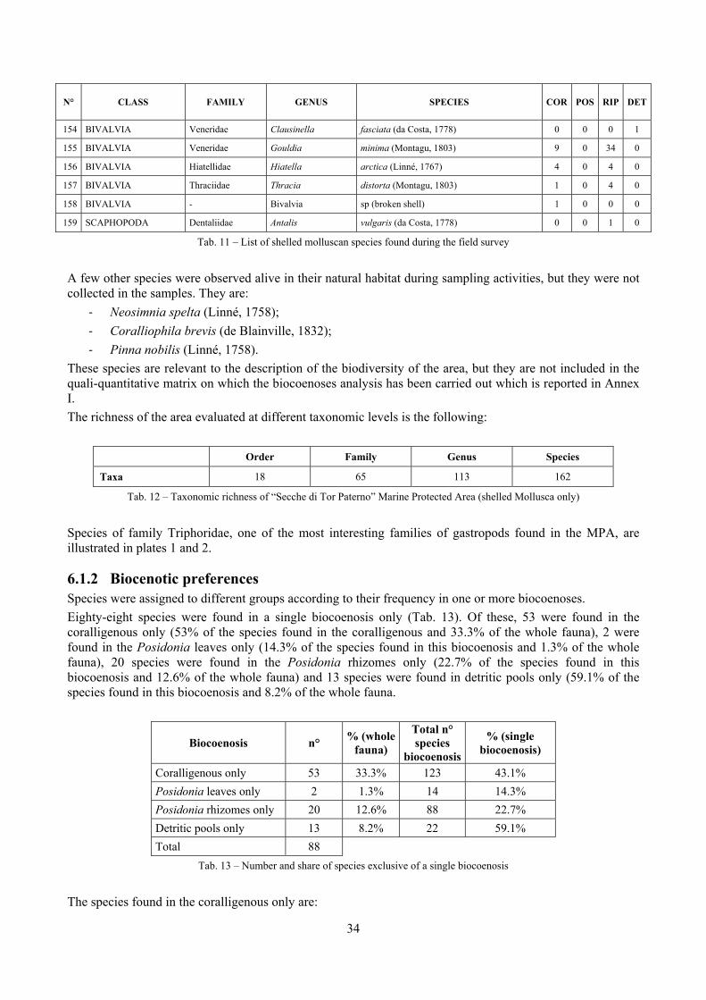
34

N° CLASS FAMILY GENUS SPECIES COR POS RIP DET

154 BIVALVIA Veneridae Clausinella fasciata (da Costa, 1778) 0 0 0 1

155 BIVALVIA Veneridae Gouldia minima (Montagu, 1803) 9 0 34 0

156 BIVALVIA Hiatellidae Hiatella arctica (Linné, 1767) 4 0 4 0

157 BIVALVIA Thraciidae Thracia distorta (Montagu, 1803) 1 0 4 0

158 BIVALVIA - Bivalvia sp (broken shell) 1 0 0 0

159 SCAPHOPODA Dentaliidae Antalis vulgaris (da Costa, 1778) 0 0 1 0

Tab. 11 – List of shelled molluscan species found during the field survey

A few other species were observed alive in their natural habitat during sampling activities, but they were not collected in the samples. They are:

‐ Neosimnia spelta (Linné, 1758); ‐ Coralliophila brevis (de Blainville, 1832); ‐ Pinna nobilis (Linné, 1758).

These species are relevant to the description of the biodiversity of the area, but they are not included in the quali-quantitative matrix on which the biocoenoses analysis has been carried out which is reported in Annex I. The richness of the area evaluated at different taxonomic levels is the following:

Order Family Genus Species

Taxa 18 65 113 162

Tab. 12 – Taxonomic richness of “Secche di Tor Paterno” Marine Protected Area (shelled Mollusca only)

Species of family Triphoridae, one of the most interesting families of gastropods found in the MPA, are illustrated in plates 1 and 2.

6.1.2 Biocenotic preferences Species were assigned to different groups according to their frequency in one or more biocoenoses. Eighty-eight species were found in a single biocoenosis only (Tab. 13). Of these, 53 were found in the coralligenous only (53% of the species found in the coralligenous and 33.3% of the whole fauna), 2 were found in the Posidonia leaves only (14.3% of the species found in this biocoenosis and 1.3% of the whole fauna), 20 species were found in the Posidonia rhizomes only (22.7% of the species found in this biocoenosis and 12.6% of the whole fauna) and 13 species were found in detritic pools only (59.1% of the species found in this biocoenosis and 8.2% of the whole fauna.

Biocoenosis n° % (whole fauna)

Total n° species

biocoenosis

% (single biocoenosis)

Coralligenous only 53 33.3% 123 43.1% Posidonia leaves only 2 1.3% 14 14.3% Posidonia rhizomes only 20 12.6% 88 22.7% Detritic pools only 13 8.2% 22 59.1% Total 88

Tab. 13 – Number and share of species exclusive of a single biocoenosis

The species found in the coralligenous only are:

35

- Lepidopleurus cajetanus - Acanthochitona crinita - Polyplacophora sp. - Diodora graeca - Emarginula octaviana - Emarginula rosea - Emarginella huzardii - Haliotis tuberculata lamellosa - Clanculus corallinus - Clanculus cruciatus - Danilia tinei - Bittium sp. 3 - Petalopoma elisabettae - Monophorus thiriotae - Similiphora similior - Cerithiopsis nofronii - Dizoniopsis coppolae - Pusillina sp. - Alvania cimex - Alvania discors - Alvania geryonia - Alvania lineata - Alvania tenera - Crisilla beniamina - Manzonia crassa - Rissoina bruguieri - Caecum subannulatum - Parastrophia asturiana - Trivia arctica - Luria lurida - Typhinellus labiatus - Euthria corneum - Pollia dorbignyi - Columbella rustica - Mitrella coccinea - Mangelia vauquelini - Raphitoma sp. 3 - Chrysallida excavata - Turbonilla gradata - Clathrella clathrata - Haminoea sp. - Weinkauffia turgidula - Lithophaga lithophaga - Chlamys flexuosa - Chlamys glabra

36

- Crassadoma multistriata - Limaria hians - Limaria tuberculata - Galeomma turtoni - Kellia suborbicularis - Montacuta sp. - Abra sp. - Bivalvia sp. (broken shell)

The species found in the Posidonia leaves only are: - Calliostoma laugieri - Rissoa auriscalpium

The species found in the Posidonia rhizomes only are: - Hanleya hanleyi - Tricolia tenuis - Smaragdia viridis - Bittium sp. 2 - Pogonodon pseudocanaricus - Cerithiopsis sp. 2 - Cerithiopsis sp. 3 - Parvioris ibizenca - Erosaria spurca - Payraudeautia intricata - Mitrella minor - Mitromorpha karpathoensis - Raphitoma sp. 4 - Mathilda gemmulata - Ondina sp. - Dacrydium hyalinum - Modiolula phaseolina - Kurtiella sp. - Gari costulata - Antalis vulgaris

The species found in the detritic pools only are: - Vitreolina incurva - Caecum armoricum - Caecum clarkii - Comarmondia gracilis - Crassopleura maravignae - Pseudotorinia architae - Turbonilla striatula - Retusa mamillata - Cylichnina crebrisculpta - Philine sp. - Hemilepton nitidum - Pteromeris corbis

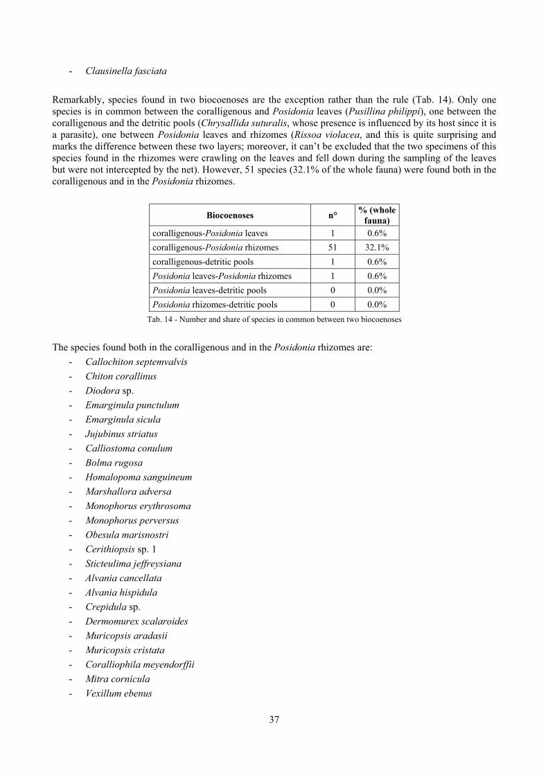
37

- Clausinella fasciata Remarkably, species found in two biocoenoses are the exception rather than the rule (Tab. 14). Only one species is in common between the coralligenous and Posidonia leaves (Pusillina philippi), one between the coralligenous and the detritic pools (Chrysallida suturalis, whose presence is influenced by its host since it is a parasite), one between Posidonia leaves and rhizomes (Rissoa violacea, and this is quite surprising and marks the difference between these two layers; moreover, it can’t be excluded that the two specimens of this species found in the rhizomes were crawling on the leaves and fell down during the sampling of the leaves but were not intercepted by the net). However, 51 species (32.1% of the whole fauna) were found both in the coralligenous and in the Posidonia rhizomes.

Biocoenoses n° % (whole fauna)

coralligenous-Posidonia leaves 1 0.6% coralligenous-Posidonia rhizomes 51 32.1% coralligenous-detritic pools 1 0.6% Posidonia leaves-Posidonia rhizomes 1 0.6% Posidonia leaves-detritic pools 0 0.0% Posidonia rhizomes-detritic pools 0 0.0%

Tab. 14 - Number and share of species in common between two biocoenoses

The species found both in the coralligenous and in the Posidonia rhizomes are:

- Callochiton septemvalvis - Chiton corallinus - Diodora sp. - Emarginula punctulum - Emarginula sicula - Jujubinus striatus - Calliostoma conulum - Bolma rugosa - Homalopoma sanguineum - Marshallora adversa - Monophorus erythrosoma - Monophorus perversus - Obesula marisnostri - Cerithiopsis sp. 1 - Sticteulima jeffreysiana - Alvania cancellata - Alvania hispidula - Crepidula sp. - Dermomurex scalaroides - Muricopsis aradasii - Muricopsis cristata - Coralliophila meyendorffii - Mitra cornicula - Vexillum ebenus

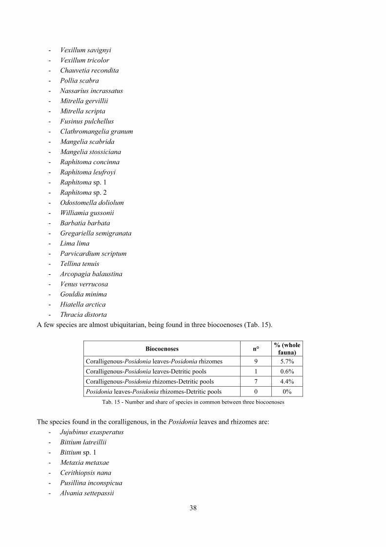
38

- Vexillum savignyi - Vexillum tricolor - Chauvetia recondita - Pollia scabra - Nassarius incrassatus - Mitrella gervillii - Mitrella scripta - Fusinus pulchellus - Clathromangelia granum - Mangelia scabrida - Mangelia stossiciana - Raphitoma concinna - Raphitoma leufroyi - Raphitoma sp. 1 - Raphitoma sp. 2 - Odostomella doliolum - Williamia gussonii - Barbatia barbata - Gregariella semigranata - Lima lima - Parvicardium scriptum - Tellina tenuis - Arcopagia balaustina - Venus verrucosa - Gouldia minima - Hiatella arctica - Thracia distorta

A few species are almost ubiquitarian, being found in three biocoenoses (Tab. 15).

Biocoenoses n° % (whole fauna)

Coralligenous-Posidonia leaves-Posidonia rhizomes 9 5.7% Coralligenous-Posidonia leaves-Detritic pools 1 0.6% Coralligenous-Posidonia rhizomes-Detritic pools 7 4.4% Posidonia leaves-Posidonia rhizomes-Detritic pools 0 0%

Tab. 15 - Number and share of species in common between three biocoenoses

The species found in the coralligenous, in the Posidonia leaves and rhizomes are:

- Jujubinus exasperatus - Bittium latreillii - Bittium sp. 1 - Metaxia metaxae - Cerithiopsis nana - Pusillina inconspicua - Alvania settepassii

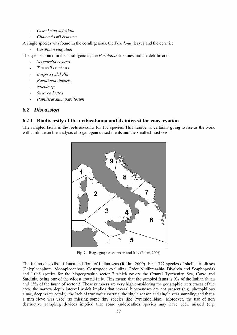
39

- Ocinebrina aciculata - Chauvetia aff brunnea

A single species was found in the coralligenous, the Posidonia leaves and the detritic: - Cerithium vulgatum

The species found in the coralligenous, the Posidonia rhizomes and the detritic are: - Scissurella costata - Turritella turbona - Euspira pulchella - Raphitoma linearis - Nucula sp. - Striarca lactea - Papillicardium papillosum

6.2 Discussion

6.2.1 Biodiversity of the malacofauna and its interest for conservation The sampled fauna in the reefs accounts for 162 species. This number is certainly going to rise as the work will continue on the analysis of organogenous sediments and the smallest fractions.

The Italian checklist of fauna and flora of Italian seas (Relini, 2009) lists 1,792 species of shelled molluscs (Polyplacophora, Monoplacophora, Gastropoda excluding Order Nudibranchia, Bivalvia and Scaphopoda) and 1,085 species for the biogeographic sector 2 which covers the Central Tyrrhenian Sea, Corse and Sardinia, being one of the widest around Italy. This means that the sampled fauna is 9% of the Italian fauna and 15% of the fauna of sector 2. These numbers are very high considering the geographic restrictness of the area, the narrow depth interval which implies that several biocoenoses are not present (e.g. photophilous algae, deep water corals), the lack of true soft substrata, the single season and single year sampling and that a 1 mm sieve was used (so missing some tiny species like Pyramidellidae). Moreover, the use of non destructive sampling devices implied that some endobenthos species may have been missed (e.g.

Fig. 9 – Biogeographic sectors around Italy (Relini, 2009)

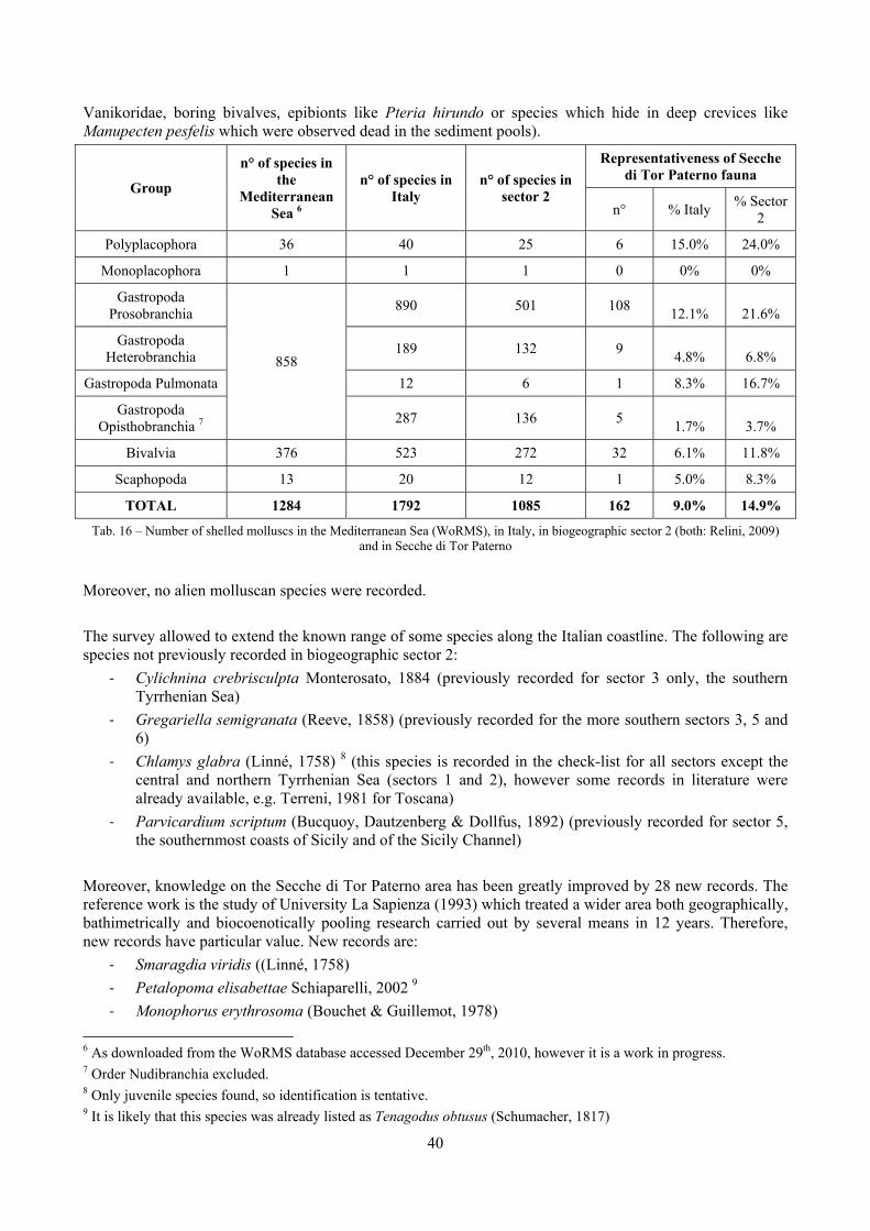
40

Vanikoridae, boring bivalves, epibionts like Pteria hirundo or species which hide in deep crevices like Manupecten pesfelis which were observed dead in the sediment pools).

Group

n° of species in the

Mediterranean Sea 6

n° of species in Italy

n° of species in sector 2

Representativeness of Secche di Tor Paterno fauna

n° % Italy % Sector 2

Polyplacophora 36 40 25 6 15.0% 24.0%

Monoplacophora 1 1 1 0 0% 0%

Gastropoda Prosobranchia

858

890 501 108 12.1% 21.6%

Gastropoda Heterobranchia 189 132 9 4.8% 6.8%

Gastropoda Pulmonata 12 6 1 8.3% 16.7%

Gastropoda Opisthobranchia 7 287 136 5 1.7% 3.7%

Bivalvia 376 523 272 32 6.1% 11.8%

Scaphopoda 13 20 12 1 5.0% 8.3%

TOTAL 1284 1792 1085 162 9.0% 14.9%

Tab. 16 – Number of shelled molluscs in the Mediterranean Sea (WoRMS), in Italy, in biogeographic sector 2 (both: Relini, 2009) and in Secche di Tor Paterno

Moreover, no alien molluscan species were recorded. The survey allowed to extend the known range of some species along the Italian coastline. The following are species not previously recorded in biogeographic sector 2:

‐ Cylichnina crebrisculpta Monterosato, 1884 (previously recorded for sector 3 only, the southern Tyrrhenian Sea)

‐ Gregariella semigranata (Reeve, 1858) (previously recorded for the more southern sectors 3, 5 and 6)

‐ Chlamys glabra (Linné, 1758) 8 (this species is recorded in the check-list for all sectors except the central and northern Tyrrhenian Sea (sectors 1 and 2), however some records in literature were already available, e.g. Terreni, 1981 for Toscana)

‐ Parvicardium scriptum (Bucquoy, Dautzenberg & Dollfus, 1892) (previously recorded for sector 5, the southernmost coasts of Sicily and of the Sicily Channel)

Moreover, knowledge on the Secche di Tor Paterno area has been greatly improved by 28 new records. The reference work is the study of University La Sapienza (1993) which treated a wider area both geographically, bathimetrically and biocoenotically pooling research carried out by several means in 12 years. Therefore, new records have particular value. New records are:

‐ Smaragdia viridis ((Linné, 1758) ‐ Petalopoma elisabettae Schiaparelli, 2002 9 ‐ Monophorus erythrosoma (Bouchet & Guillemot, 1978)

6 As downloaded from the WoRMS database accessed December 29th, 2010, however it is a work in progress. 7 Order Nudibranchia excluded. 8 Only juvenile species found, so identification is tentative. 9 It is likely that this species was already listed as Tenagodus obtusus (Schumacher, 1817)

41

‐ Monophorus thiriotae Bouchet, 1985 ‐ Obesula marisnostri Bouchet, 1985 ‐ Pogonodon pseudocanaricus (Bouchet, 1985) ‐ Caecum armoricum De Folin, 1869 ‐ Caecum clarkii Carpenter, 1859 ‐ Chauvetia recondita (Brugnone, 1873) ‐ Pollia scabra Locard, 1892 ‐ Mitrella coccinea (Philippi, 1836) ‐ Mitromorpha karpathoensis (Nordsieck, 1969) ‐ Raphitoma concinna (Scacchi, 1836) ‐ Pseudotorinia architae (Costa O.G., 1841) ‐ Mathilda gemmulata Semper, 1865 ‐ Turbonilla gradata Bucquoy, Dautzenberg & Dollfus, 1883 ‐ Clathrella clathrata (Philippi, 1844) ‐ Cylichnina crebrisculpta Monterosato, 1884 ‐ Gregariella semigranata (Reeve, 1858) ‐ Modiolula phaseolina (Philippi, 1844) ‐ Chlamys flexuosa (Poli, 1795) ‐ Chlamys glabra (Linné, 1758) ‐ Limaria tuberculata (Olivi, 1792) ‐ Hemilepton nitidum (Turton, 1822) ‐ Tellina tenuis Da Costa, 1778 ‐ Gari costulata (Turton, 1822) ‐ Clausinella fasciata (Da Costa, 1778) ‐ Antalis vulgaris (Da Costa, 1778)

More new records may hide in groups with difficult taxonomy like Bittium, Cerithiopsidae, Mangelia, Raphitoma, which couln’t be assigned to a taxon with certainty. It is important to highlight the presence of the following species of conservation interest:

‐ Erosaria spurca (Linné, 1758) (Gastropoda: Cypraeidae) This species is a member of the family Cypraeidae, much sought after by collectors. For this reason, all Mediterranean autoctonous species of this family are protected. This species is enlisted in Appendix II “Strictly protected fauna species” of the Bern Convention and in Annex II to the Protocol Concerning Specially Protected Areas and Biological Diversity in the Mediterranean of the Barcelona Convention which is devoted to endangered species. A single adult living specimen has been found. A few other dead specimens were found, but the species looks to be very rare in the Area while it is more common in the southern Mediterranean Sea.

‐ Luria lurida (Linné, 1758) (Gastropoda: Cypraeidae) This species belongs to the same family as Erosaria spurca and enjoys the same degree of protection. It is enlisted in Appendix II “Strictly protected fauna species” of the Bern Convention and in the Annex II to the Protocol Concerning Specially Protected Areas and Biological Diversity in the Mediterranean of the Barcelona Convention too. A single living juvenile specimen has been found. A few dead specimens were collected. Again the species is rare in the Area, while it is usually more common in the shallows in coastal waters of most of the Mediterranean Sea, with the exception of its coldest parts (e.g.: North-Eastern Adriatic Sea).

‐ Lithophaga lithophaga (Linné, 1758) (Bivalvia: Mytilidae)

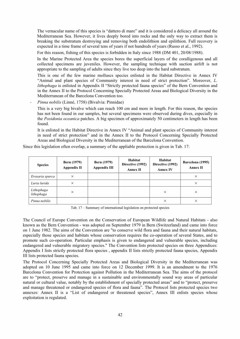
42

The vernacular name of this species is “dattero di mare” and it is considered a delicacy all around the Mediterranean Sea. However, it lives deeply bored into rocks and the only way to extract them is breaking the substratum destroying and removing both endolithion and epilithion. Full recovery is expected in a time frame of several tens of years if not hundreds of years (Russo et al., 1992). For this reason, fishing of this species is forbidden in Italy since 1988 (DM 401, 20/08/1988). In the Marine Protected Area the species bores the superficial layers of the coralligenous and all collected specimens are juveniles. However, the sampling technique with suction airlift is not appropriate to the sampling of adults since they live too deep into the hard substratum. This is one of the few marine molluscs species enlisted in the Habitat Directive in Annex IV “Animal and plant species of Community interest in need of strict protection”. Moreover, L. lithophaga is enlisted in Appendix II “Strictly protected fauna species” of the Bern Convention and in the Annex II to the Protocol Concerning Specially Protected Areas and Biological Diversity in the Mediterranean of the Barcelona Convention too.

‐ Pinna nobilis (Linné, 1758) (Bivalvia: Pinnidae) This is a very big bivalve which can reach 100 cm and more in length. For this reason, the species has not been found in our samples, but several specimens were observed during dives, especially in the Posidonia oceanica patches. A big specimen of approximately 50 centimeters in length has been found. It is enlisted in the Habitat Directive in Annex IV “Animal and plant species of Community interest in need of strict protection” and in the Annex II to the Protocol Concerning Specially Protected Areas and Biological Diversity in the Mediterranean of the Barcelona Convention.

Since this legislation often overlap, a summary of the appliable protection is given in Tab. 17:

Species Bern (1979) Appendix II

Bern (1979) Appendix III

Habitat Directive (1992)

Annex II

Habitat Directive (1992)

Annex IV

Barcelona (1995) Annex II

Erosaria spurca × × Luria lurida × × Lithophaga lithophaga × × ×

Pinna nobilis × × Tab. 17 – Summary of international legislation on protected species

The Council of Europe Convention on the Conservation of European Wildlife and Natural Habitats - also known as the Bern Convention - was adopted on September 1979 in Bern (Switzerland) and came into force on 1 June 1982. The aims of the Convention are "to conserve wild flora and fauna and their natural habitats, especially those species and habitats whose conservation requires the co-operation of several States, and to promote such co-operation. Particular emphasis is given to endangered and vulnerable species, including endangered and vulnerable migratory species." The Convention lists protected species on three Appendices: Appendix I lists strictly protected flora species , appendix II lists strictly protected fauna species, Appendix III lists protected fauna species. The Protocol Concerning Specially Protected Areas and Biological Diversity in the Mediterranean was adopted on 10 June 1995 and came into force on 12 December 1999. It is an amendment to the 1976 Barcelona Convention for Protection against Pollution in the Mediterranean Sea. The aims of the protocol are to “protect, preserve and manage in a sustainable and environmentally sound way areas of particular natural or cultural value, notably by the establishment of specially protected areas” and to “protect, preserve and manage threatened or endangered species of flora and fauna”. The Protocol lists protected species two annexes: Annex II is a “List of endangered or threatened species”, Annex III enlists species whose exploitation is regulated.

43

The Habitats Directive (more formally known as Council Directive 92/43/EEC on the Conservation of natural habitats and of wild fauna and flora) is a European Union directive adopted in 1992 as an EU response to the Berne Convention. It aims to protect some 220 habitats and approximately 1000 species listed in the directive's Annexes. These are species and habitats which are considered to be of European interest, following criteria given in the directive. The directive lists protected species in three annexes: Annex II covers “Animal and plant species of community interest whose conservation requires the designation of special areas of conservation”, Annex IV covers “Animal and plant species of community interest in need of strict protection”, while Annex V lists species “of community interest whose taking in the wild and exploitation may be subject to management measures”. Moreover, Secche di Tor Paterno were the source of material which lead to the description of a few species of shelled molluscs:

‐ Cerithiopsis nofronii Amati, 1987 (Gastropoda: Cerithiopsidae) The locus typicus of this species is Bocche di Bonifacio. Two lots coming from the Tor Paterno reefs were designated as paratypes of this species. A single, but living, specimen has been found in the survey. A few other dead specimens were found in the sorting of thanatocoenosis samples collected before the survey. It seems to be a very rare species in the investigated area. It may prefer deeper waters.

‐ Alvania settepassii Amati & Nofroni, 1985 (Gastropoda: Rissoidae) The locus typicus of this species is the Marine Protected Area. This species is common in the thanatocoenosis sediments, but it is uncommon alive. However, 29 living specimens were found, both juveniles and adults, confirming the presence of a population in the area. This species is present in other parts of the Tyrrhenian Sea and specimens tentatively assigned to this taxon are reported from the Jonian coasts of Puglia (Trono, 2006).

6.2.2 Biocenotic preferences The number of species exclusive of a single biocoenosis is remarkably high. However, only a few species are known for being restricted to the biocoenosis in literature. Several species (Triphoridae, Cerithiopsidae, Pyramidellidae) are parasites or extremely specialized predators and are expected where their host lives. However, for most species the host is not known. Between the species characteristic of the coralligenous there are Danilia tinei (Palazzi & Villari (2001) cite specimens from the rhizomes of dense Posidonia meadows and caves, but these records are occasional in literature), Alvania tenera (cfr. Piani, 1979), Mitrella coccinea. The coralligenous host a good number of exclusive species (19, 35.8%) which feed on microalgae and therefore depend on light, despite dim, for survival (e.g. Polyplacophora, Trochidae, Rissoidae). Rissoa auriscalpium is a characteristic and exclusive species of Posidonia leaves and it is more common in shallow and sheltered water. Between the species found in the rhizomes only, most are carnivorous or parasites (11, 55.5%). Between the few species which feed on microalgae there are Tricolia tenuis and Smaragdia viridis which are usually associated to the leaves. Their presence can be justified with the nictemeral migrations on the plant axis which is already described in literature for T. pullus (Russo et al., 1984). Several species were exclusively found in the detritic pools. These pools are a markedly different habitat from the others and this justifies the high percentage of species found only in them. The main consequence is that sampling these pools, which at first sight seem lifeless, brought an important addition on the knowledge of the biodiversity of Secche di Tor Paterno. Between these, some are Comarmondia gracilis and Crassopleura maravignae, two predators which hide in the sediment. The remarkable high number of species in common between the coralligenous and the Posidonia rhizomes are peculiarly polarized towards parasites and carnivorous species: 31 species, 60.7%! These species are usually pretty vagile and probably find adequate prey or host in both sciaphilous environments.

44

Between the almost ubiquitarian species present in three biocoenoses, two main groups are recognizable. The first is the group of species affiliated to light both because they eat microalgae (e.g. Bittium, Rissoidae) or because they are vagile species not strictly sciaphilous (e.g. Muricidae). This group thrives in the coralligenous and Posidonia leaves and rhizomes. The second is a group of mainly infaunal species associated to soft substrata which thrives not only in the detritic pools, but in the coralligenous and rhizomes too where small pockets of sediment are present. The only species found in the three most diverse biocoenoses, coralligenous, Posidonia leaves and detritic pools, Cerithium vulgatum, should be considered dubious since morphological evidence suggest the species found in the detritic pools may not be C. vulgatum but a different species.

45

7 Biocoenoses characterization Sampling was carried out in the infralittoral level of the reefs which is characterized by biocoenoses which are installed on rock emerging from the surrounding circalittoral soft substrata. At this level, the reefs host four different biocoenoses:

- Biocoenosis of the Posidonia oceanica meadows (“HP”, Pérès & Picard, 1964), which is characterized in its definition by the foliar layer species assemblages;

- Biocoenosis of the rhizomes epifauna of Posidonia oceanica, which can be identified as a particular form of the Coralligenous biocoenosis (“C”, Pérès & Picard, 1964) due to its sciaphilous conditions and that can be related to the precoralligenous;

- Biocoenosis of the coralligenous (“C”, Pérès & Picard, 1964), in its typical aspect, which hosts a few different facies;

- Biocoenosis of the Coastal Detritic (“DC”, Pérès & Picard, 1964). A few issues have to be highlighted. First, water turbidity is very variable due to the estaury of the Tevere river a few kilometers northwards often causes low water transparency, especially during floods. In periods of low rainfall visibility can be good (up to 20 meters) and affected by turbidity brought by bottom currents. This issue combined with the depth (reef tops are at 18 meters and rapidly decrease to lower depths) allow biocoenoses with different light requirements to live one close to each other. On the reefs the conditions allow the existence of Posidonia oceanica and of the coralligenous side to side and this brings to the existence of ecotones and ecoclines which add much to the richness of the area. Second, the Posidonia oceanica meadows are a “carrefour biocenotique” (Bianchi et al. 1989) and we have investigated two different levels: the leaves and the rhizomes. The former is a photophilous environment while the latter is a sciaphilous environment with encrusting coralline algae and has some characters of an enclave of coralligenous in the Posidonia oceanica meadow (Pérès and Picard 1964). Last, the Posidonia rhizomes are characterized by the presence of fine sediment which may allow the settlement of species with affinity to soft substrata. The quantity of sediment depends upon whether Posidonia settles on hard or soft substrata, but it is anyway much higher than in the coralligenous. This can be mostly related to the effect of the foliar layer which reduces water hydrodynamism. A similar effect can be found in small crevices of the coralligenous but it is much more random distributed. The data analysis was therefore aimed at understanding to which extent these biocoenoses host different molluscan species assemblages and which taxa make the difference. This is the basis for further analysis of each biocoenosis and comparison with other data sets.

7.1 Results One of the main problems was to verify to which extent the molluscan assemblages differed in any way between biocoenoses. In other words: do the biocoenoses host typical molluscan assemblages? Then to answer to the question the data were treated with two different approaches:

1. Analysis of data with an univariate approach, using diversity indices to describe each sample; 2. Analysis of data with a multivariate approach, using the full quali-quantitative data matrix shown in

Annex I.

7.1.1 Univariate approach The computed indices were (see chapter 4.4 “Biodiversity indices” for details):

‐ Indices of species richness: o S, number of species; o d, Margalef’s species richness;

‐ Indices of diversity: o H’, Shannon index; o λ, Simpson index.

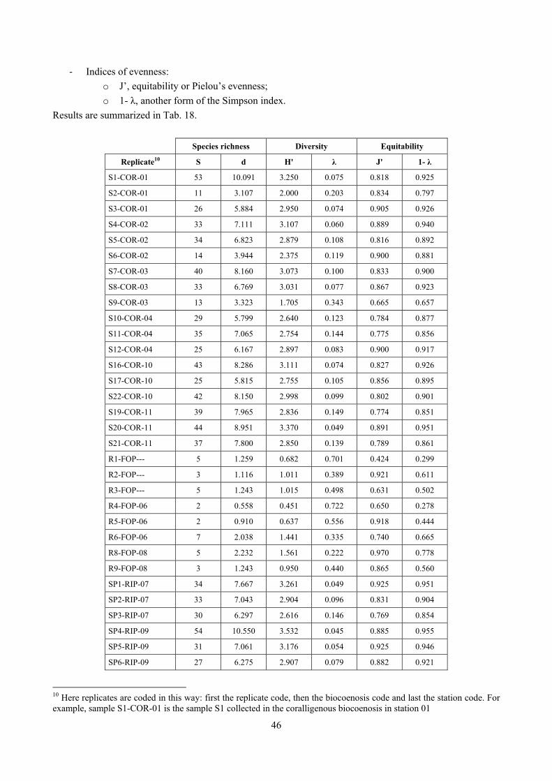
46

‐ Indices of evenness: o J’, equitability or Pielou’s evenness; o 1- λ, another form of the Simpson index.

Results are summarized in Tab. 18.

Species richness Diversity Equitability

Replicate10 S d H' λ J' 1- λ

S1-COR-01 53 10.091 3.250 0.075 0.818 0.925

S2-COR-01 11 3.107 2.000 0.203 0.834 0.797

S3-COR-01 26 5.884 2.950 0.074 0.905 0.926

S4-COR-02 33 7.111 3.107 0.060 0.889 0.940

S5-COR-02 34 6.823 2.879 0.108 0.816 0.892

S6-COR-02 14 3.944 2.375 0.119 0.900 0.881

S7-COR-03 40 8.160 3.073 0.100 0.833 0.900

S8-COR-03 33 6.769 3.031 0.077 0.867 0.923

S9-COR-03 13 3.323 1.705 0.343 0.665 0.657

S10-COR-04 29 5.799 2.640 0.123 0.784 0.877

S11-COR-04 35 7.065 2.754 0.144 0.775 0.856

S12-COR-04 25 6.167 2.897 0.083 0.900 0.917

S16-COR-10 43 8.286 3.111 0.074 0.827 0.926

S17-COR-10 25 5.815 2.755 0.105 0.856 0.895

S22-COR-10 42 8.150 2.998 0.099 0.802 0.901

S19-COR-11 39 7.965 2.836 0.149 0.774 0.851

S20-COR-11 44 8.951 3.370 0.049 0.891 0.951

S21-COR-11 37 7.800 2.850 0.139 0.789 0.861

R1-FOP--- 5 1.259 0.682 0.701 0.424 0.299

R2-FOP--- 3 1.116 1.011 0.389 0.921 0.611

R3-FOP--- 5 1.243 1.015 0.498 0.631 0.502

R4-FOP-06 2 0.558 0.451 0.722 0.650 0.278

R5-FOP-06 2 0.910 0.637 0.556 0.918 0.444

R6-FOP-06 7 2.038 1.441 0.335 0.740 0.665

R8-FOP-08 5 2.232 1.561 0.222 0.970 0.778

R9-FOP-08 3 1.243 0.950 0.440 0.865 0.560

SP1-RIP-07 34 7.667 3.261 0.049 0.925 0.951

SP2-RIP-07 33 7.043 2.904 0.096 0.831 0.904

SP3-RIP-07 30 6.297 2.616 0.146 0.769 0.854

SP4-RIP-09 54 10.550 3.532 0.045 0.885 0.955

SP5-RIP-09 31 7.061 3.176 0.054 0.925 0.946

SP6-RIP-09 27 6.275 2.907 0.079 0.882 0.921

10 Here replicates are coded in this way: first the replicate code, then the biocoenosis code and last the station code. For example, sample S1-COR-01 is the sample S1 collected in the coralligenous biocoenosis in station 01

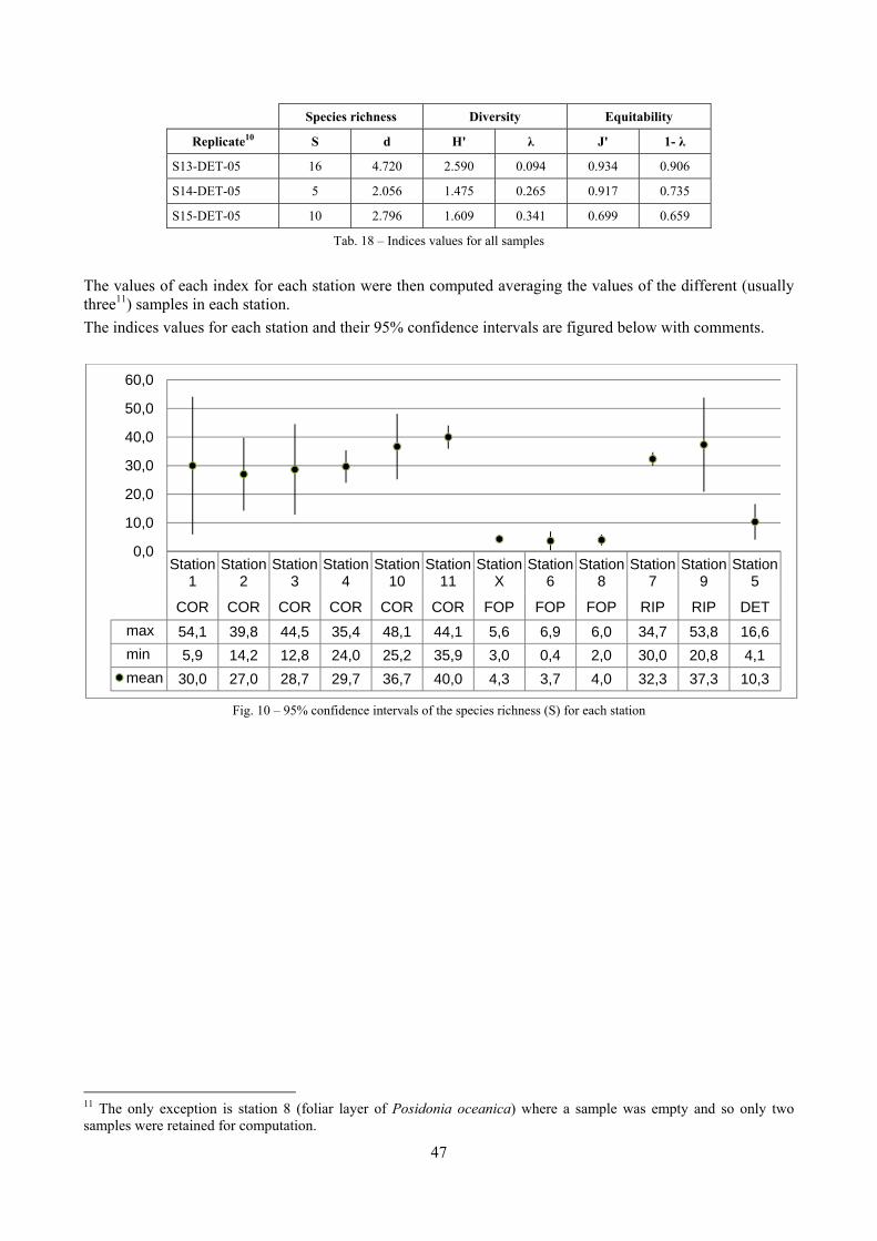
47

Species richness Diversity Equitability

Replicate10 S d H' λ J' 1- λ

S13-DET-05 16 4.720 2.590 0.094 0.934 0.906

S14-DET-05 5 2.056 1.475 0.265 0.917 0.735

S15-DET-05 10 2.796 1.609 0.341 0.699 0.659

Tab. 18 – Indices values for all samples

The values of each index for each station were then computed averaging the values of the different (usually three11) samples in each station. The indices values for each station and their 95% confidence intervals are figured below with comments.

Fig. 10 – 95% confidence intervals of the species richness (S) for each station

11 The only exception is station 8 (foliar layer of Posidonia oceanica) where a sample was empty and so only two samples were retained for computation.

Station1

Station2

Station3

Station4

Station10

Station11

StationX

Station6

Station8

Station7

Station9

Station5

COR COR COR COR COR COR FOP FOP FOP RIP RIP DETmax 54,1 39,8 44,5 35,4 48,1 44,1 5,6 6,9 6,0 34,7 53,8 16,6min 5,9 14,2 12,8 24,0 25,2 35,9 3,0 0,4 2,0 30,0 20,8 4,1mean 30,0 27,0 28,7 29,7 36,7 40,0 4,3 3,7 4,0 32,3 37,3 10,3

0,0

10,0

20,0

30,0

40,0

50,0

60,0

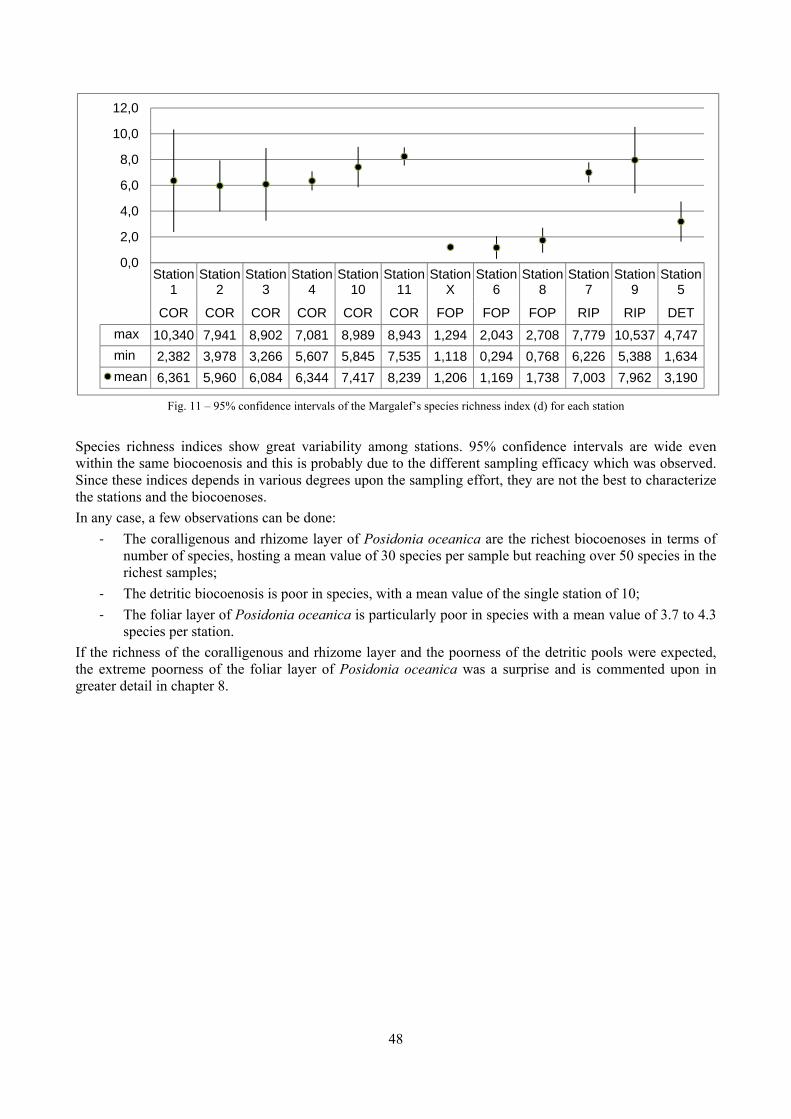
48

Fig. 11 – 95% confidence intervals of the Margalef’s species richness index (d) for each station

Species richness indices show great variability among stations. 95% confidence intervals are wide even within the same biocoenosis and this is probably due to the different sampling efficacy which was observed. Since these indices depends in various degrees upon the sampling effort, they are not the best to characterize the stations and the biocoenoses. In any case, a few observations can be done:

‐ The coralligenous and rhizome layer of Posidonia oceanica are the richest biocoenoses in terms of number of species, hosting a mean value of 30 species per sample but reaching over 50 species in the richest samples;

‐ The detritic biocoenosis is poor in species, with a mean value of the single station of 10; ‐ The foliar layer of Posidonia oceanica is particularly poor in species with a mean value of 3.7 to 4.3

species per station. If the richness of the coralligenous and rhizome layer and the poorness of the detritic pools were expected, the extreme poorness of the foliar layer of Posidonia oceanica was a surprise and is commented upon in greater detail in chapter 8.

Station1

Station2

Station3

Station4

Station10

Station11

StationX

Station6

Station8

Station7

Station9

Station5

COR COR COR COR COR COR FOP FOP FOP RIP RIP DETmax 10,340 7,941 8,902 7,081 8,989 8,943 1,294 2,043 2,708 7,779 10,537 4,747min 2,382 3,978 3,266 5,607 5,845 7,535 1,118 0,294 0,768 6,226 5,388 1,634mean 6,361 5,960 6,084 6,344 7,417 8,239 1,206 1,169 1,738 7,003 7,962 3,190

0,0

2,0

4,0

6,0

8,0

10,0

12,0

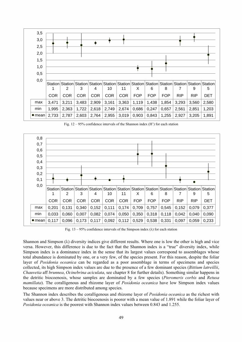
49

Fig. 12 – 95% confidence intervals of the Shannon index (H’) for each station

Fig. 13 – 95% confidence intervals of the Simpson index (λ) for each station

Shannon and Simpson (λ) diversity indices give different results. Where one is low the other is high and vice versa. However, this difference is due to the fact that the Shannon index is a “true” diversity index, while Simpson index is a dominance index in the sense that its largest values correspond to assemblages whose total abundance is dominated by one, or a very few, of the species present. For this reason, despite the foliar layer of Posidonia oceanica can be regarded as a poor assemblage in terms of specimens and species collected, its high Simpson index values are due to the presence of a few dominant species (Bittium latreillii, Chauvetia aff brunnea, Ocinebrina aciculata, see chapter 8 for further details). Something similar happens in the detritic biocoenosis, whose samples are dominated by a few species (Pteromeris corbis and Retusa mamillata). The coralligenous and rhizome layer of Posidonia oceanica have low Simpson index values because specimens are more distributed among species. The Shannon index describes the coralligenous and rhizome layer of Posidonia oceanica as the richest with values near or above 3. The detritic biocoenosis is poorer with a mean value of 1.891 while the foliar layer of Posidonia oceanica is the poorest with Shannon index values between 0.843 and 1.255.

Station1

Station2

Station3

Station4

Station10

Station11

StationX

Station6

Station8

Station7

Station9

Station5

COR COR COR COR COR COR FOP FOP FOP RIP RIP DETmax 3,471 3,211 3,483 2,909 3,161 3,363 1,119 1,438 1,854 3,293 3,560 2,580min 1,995 2,363 1,722 2,618 2,749 2,674 0,686 0,247 0,657 2,561 2,851 1,203mean 2,733 2,787 2,603 2,764 2,955 3,019 0,903 0,843 1,255 2,927 3,205 1,891

0,00,51,01,52,02,53,03,5

Station1

Station2

Station3

Station4

Station10

Station11

StationX

Station6

Station8

Station7

Station9

Station5

COR COR COR COR COR COR FOP FOP FOP RIP RIP DETmax 0,201 0,131 0,340 0,152 0,111 0,174 0,709 0,757 0,545 0,152 0,079 0,377min 0,033 0,060 0,007 0,082 0,074 0,050 0,350 0,318 0,118 0,042 0,040 0,090mean 0,117 0,096 0,173 0,117 0,092 0,112 0,529 0,538 0,331 0,097 0,059 0,233

0,00,10,20,30,40,50,60,70,8

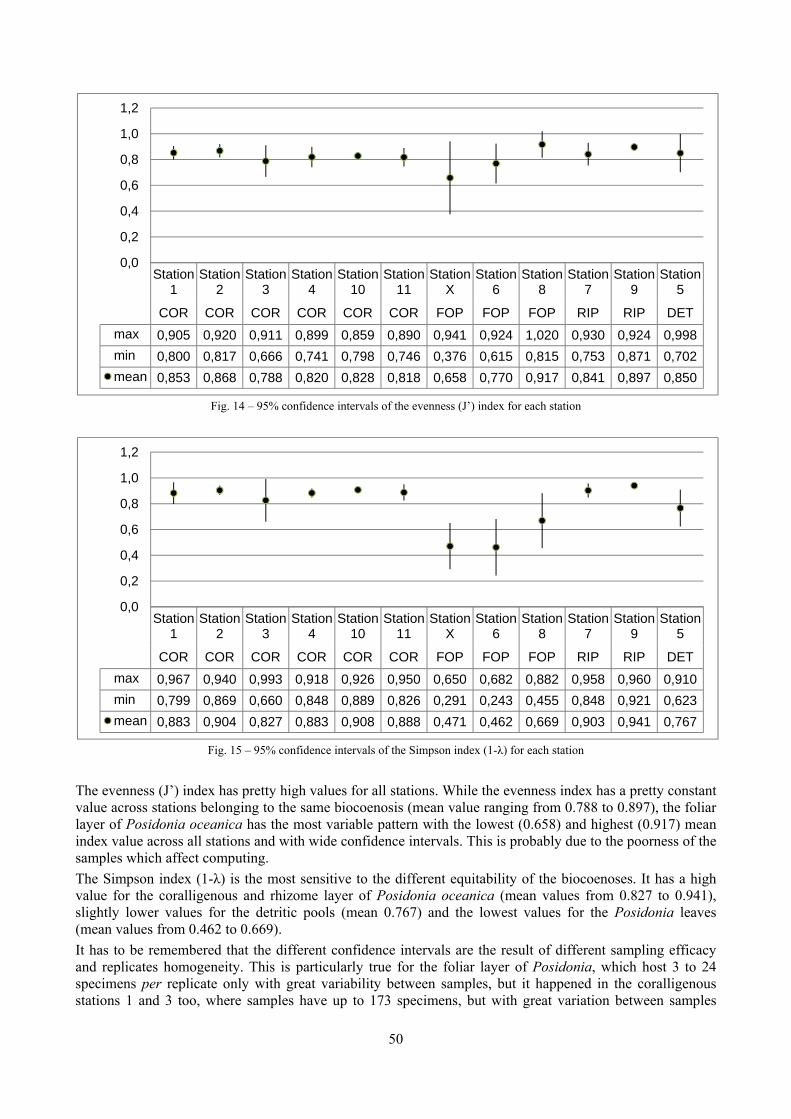
50

Fig. 14 – 95% confidence intervals of the evenness (J’) index for each station

Fig. 15 – 95% confidence intervals of the Simpson index (1-λ) for each station

The evenness (J’) index has pretty high values for all stations. While the evenness index has a pretty constant value across stations belonging to the same biocoenosis (mean value ranging from 0.788 to 0.897), the foliar layer of Posidonia oceanica has the most variable pattern with the lowest (0.658) and highest (0.917) mean index value across all stations and with wide confidence intervals. This is probably due to the poorness of the samples which affect computing. The Simpson index (1-λ) is the most sensitive to the different equitability of the biocoenoses. It has a high value for the coralligenous and rhizome layer of Posidonia oceanica (mean values from 0.827 to 0.941), slightly lower values for the detritic pools (mean 0.767) and the lowest values for the Posidonia leaves (mean values from 0.462 to 0.669). It has to be remembered that the different confidence intervals are the result of different sampling efficacy and replicates homogeneity. This is particularly true for the foliar layer of Posidonia, which host 3 to 24 specimens per replicate only with great variability between samples, but it happened in the coralligenous stations 1 and 3 too, where samples have up to 173 specimens, but with great variation between samples

Station1

Station2

Station3

Station4

Station10

Station11

StationX

Station6

Station8

Station7

Station9

Station5

COR COR COR COR COR COR FOP FOP FOP RIP RIP DETmax 0,905 0,920 0,911 0,899 0,859 0,890 0,941 0,924 1,020 0,930 0,924 0,998min 0,800 0,817 0,666 0,741 0,798 0,746 0,376 0,615 0,815 0,753 0,871 0,702mean 0,853 0,868 0,788 0,820 0,828 0,818 0,658 0,770 0,917 0,841 0,897 0,850

0,0

0,2

0,4

0,6

0,8

1,0

1,2

Station1

Station2

Station3

Station4

Station10

Station11

StationX

Station6

Station8

Station7

Station9

Station5

COR COR COR COR COR COR FOP FOP FOP RIP RIP DETmax 0,967 0,940 0,993 0,918 0,926 0,950 0,650 0,682 0,882 0,958 0,960 0,910min 0,799 0,869 0,660 0,848 0,889 0,826 0,291 0,243 0,455 0,848 0,921 0,623mean 0,883 0,904 0,827 0,883 0,908 0,888 0,471 0,462 0,669 0,903 0,941 0,767

0,0

0,2

0,4

0,6

0,8

1,0

1,2

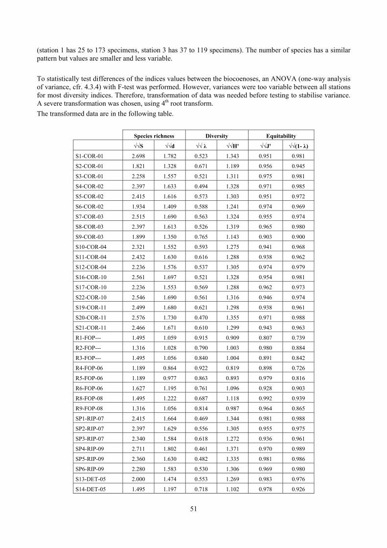
51

(station 1 has 25 to 173 specimens, station 3 has 37 to 119 specimens). The number of species has a similar pattern but values are smaller and less variable. To statistically test differences of the indices values between the biocoenoses, an ANOVA (one-way analysis of variance, cfr. 4.3.4) with F-test was performed. However, variances were too variable between all stations for most diversity indices. Therefore, transformation of data was needed before testing to stabilise variance. A severe transformation was chosen, using 4th root transform. The transformed data are in the following table.

Species richness Diversity Equitability

√√S √√d √√ λ √√H' √√J' √√(1- λ)

S1-COR-01 2.698 1.782 0.523 1.343 0.951 0.981

S2-COR-01 1.821 1.328 0.671 1.189 0.956 0.945

S3-COR-01 2.258 1.557 0.521 1.311 0.975 0.981

S4-COR-02 2.397 1.633 0.494 1.328 0.971 0.985

S5-COR-02 2.415 1.616 0.573 1.303 0.951 0.972

S6-COR-02 1.934 1.409 0.588 1.241 0.974 0.969

S7-COR-03 2.515 1.690 0.563 1.324 0.955 0.974

S8-COR-03 2.397 1.613 0.526 1.319 0.965 0.980

S9-COR-03 1.899 1.350 0.765 1.143 0.903 0.900

S10-COR-04 2.321 1.552 0.593 1.275 0.941 0.968

S11-COR-04 2.432 1.630 0.616 1.288 0.938 0.962

S12-COR-04 2.236 1.576 0.537 1.305 0.974 0.979

S16-COR-10 2.561 1.697 0.521 1.328 0.954 0.981

S17-COR-10 2.236 1.553 0.569 1.288 0.962 0.973

S22-COR-10 2.546 1.690 0.561 1.316 0.946 0.974

S19-COR-11 2.499 1.680 0.621 1.298 0.938 0.961

S20-COR-11 2.576 1.730 0.470 1.355 0.971 0.988

S21-COR-11 2.466 1.671 0.610 1.299 0.943 0.963

R1-FOP--- 1.495 1.059 0.915 0.909 0.807 0.739

R2-FOP--- 1.316 1.028 0.790 1.003 0.980 0.884

R3-FOP--- 1.495 1.056 0.840 1.004 0.891 0.842

R4-FOP-06 1.189 0.864 0.922 0.819 0.898 0.726

R5-FOP-06 1.189 0.977 0.863 0.893 0.979 0.816

R6-FOP-06 1.627 1.195 0.761 1.096 0.928 0.903

R8-FOP-08 1.495 1.222 0.687 1.118 0.992 0.939

R9-FOP-08 1.316 1.056 0.814 0.987 0.964 0.865

SP1-RIP-07 2.415 1.664 0.469 1.344 0.981 0.988

SP2-RIP-07 2.397 1.629 0.556 1.305 0.955 0.975

SP3-RIP-07 2.340 1.584 0.618 1.272 0.936 0.961

SP4-RIP-09 2.711 1.802 0.461 1.371 0.970 0.989

SP5-RIP-09 2.360 1.630 0.482 1.335 0.981 0.986

SP6-RIP-09 2.280 1.583 0.530 1.306 0.969 0.980

S13-DET-05 2.000 1.474 0.553 1.269 0.983 0.976

S14-DET-05 1.495 1.197 0.718 1.102 0.978 0.926

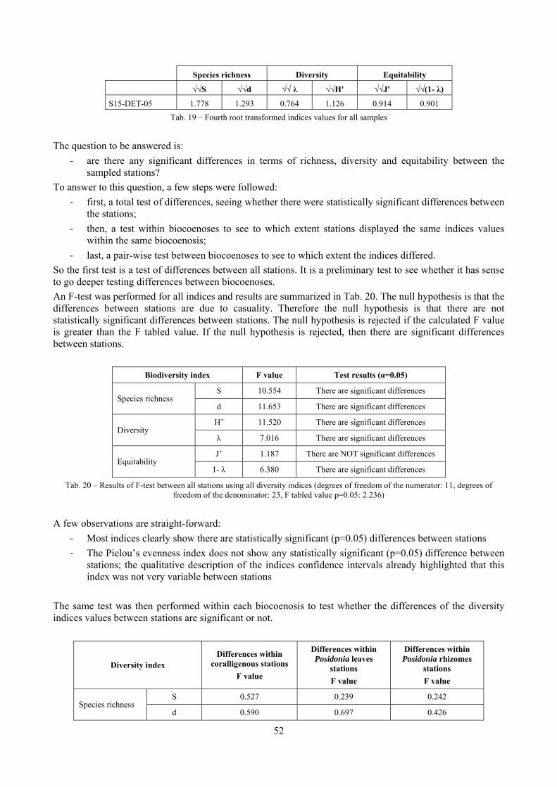
52

Species richness Diversity Equitability

√√S √√d √√ λ √√H' √√J' √√(1- λ)

S15-DET-05 1.778 1.293 0.764 1.126 0.914 0.901 Tab. 19 – Fourth root transformed indices values for all samples

The question to be answered is:

‐ are there any significant differences in terms of richness, diversity and equitability between the sampled stations?

To answer to this question, a few steps were followed: ‐ first, a total test of differences, seeing whether there were statistically significant differences between

the stations; ‐ then, a test within biocoenoses to see to which extent stations displayed the same indices values

within the same biocoenosis; ‐ last, a pair-wise test between biocoenoses to see to which extent the indices differed.

So the first test is a test of differences between all stations. It is a preliminary test to see whether it has sense to go deeper testing differences between biocoenoses. An F-test was performed for all indices and results are summarized in Tab. 20. The null hypothesis is that the differences between stations are due to casuality. Therefore the null hypothesis is that there are not statistically significant differences between stations. The null hypothesis is rejected if the calculated F value is greater than the F tabled value. If the null hypothesis is rejected, then there are significant differences between stations.

Biodiversity index F value Test results (α=0.05)

Species richness S 10.554 There are significant differences

d 11.653 There are significant differences

Diversity H’ 11.520 There are significant differences

λ 7.016 There are significant differences

Equitability J’ 1.187 There are NOT significant differences

1- λ 6.380 There are significant differences

Tab. 20 – Results of F-test between all stations using all diversity indices (degrees of freedom of the numerator: 11, degrees of freedom of the denominator: 23, F tabled value p=0.05: 2.236)

A few observations are straight-forward:

‐ Most indices clearly show there are statistically significant (p=0.05) differences between stations ‐ The Pielou’s evenness index does not show any statistically significant (p=0.05) difference between

stations; the qualitative description of the indices confidence intervals already highlighted that this index was not very variable between stations

The same test was then performed within each biocoenosis to test whether the differences of the diversity indices values between stations are significant or not.

Diversity index Differences within

coralligenous stations F value

Differences within Posidonia leaves

stations F value

Differences within Posidonia rhizomes

stations F value

Species richness S 0.527 0.239 0.242

d 0.590 0.697 0.426

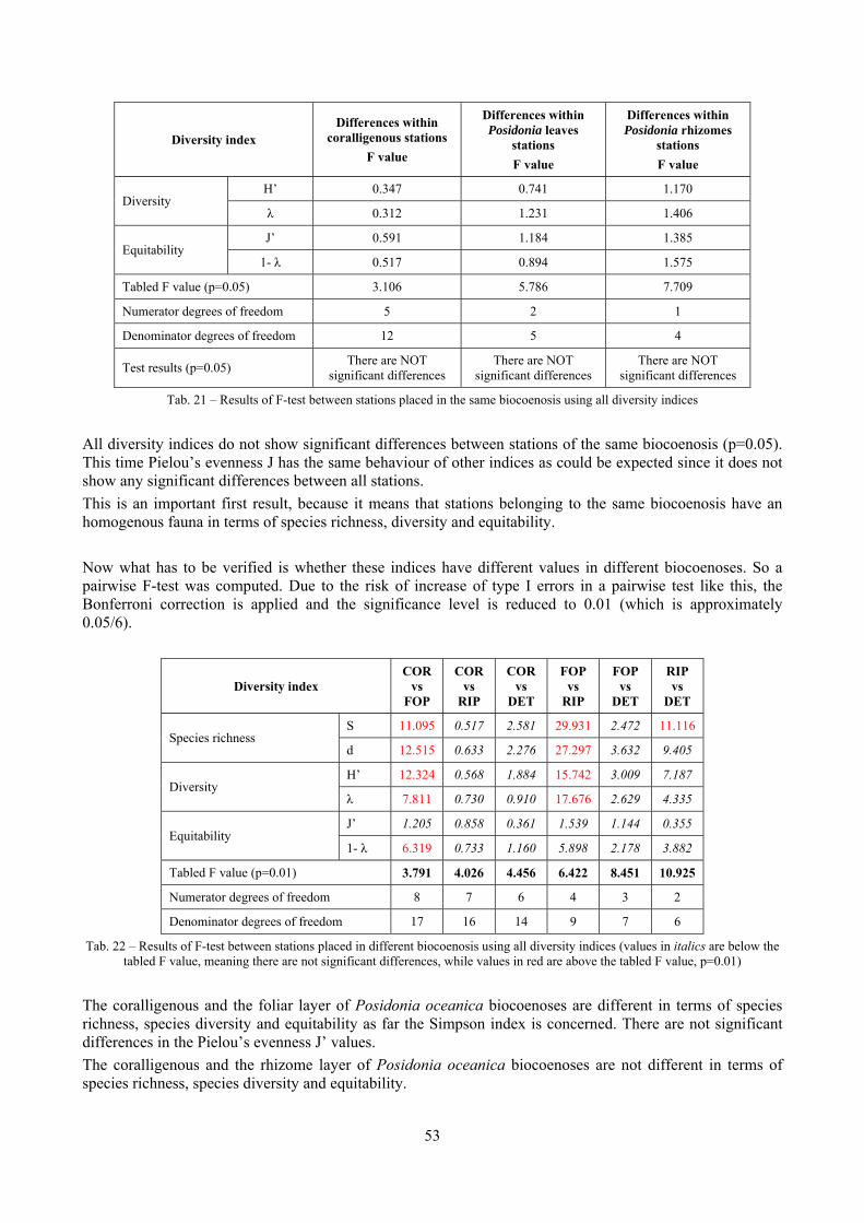
53

Diversity index Differences within

coralligenous stations F value

Differences within Posidonia leaves

stations F value

Differences within Posidonia rhizomes

stations F value

Diversity H’ 0.347 0.741 1.170

λ 0.312 1.231 1.406

Equitability J’ 0.591 1.184 1.385

1- λ 0.517 0.894 1.575

Tabled F value (p=0.05) 3.106 5.786 7.709

Numerator degrees of freedom 5 2 1

Denominator degrees of freedom 12 5 4

Test results (p=0.05) There are NOT significant differences

There are NOT significant differences

There are NOT significant differences

Tab. 21 – Results of F-test between stations placed in the same biocoenosis using all diversity indices

All diversity indices do not show significant differences between stations of the same biocoenosis (p=0.05). This time Pielou’s evenness J has the same behaviour of other indices as could be expected since it does not show any significant differences between all stations. This is an important first result, because it means that stations belonging to the same biocoenosis have an homogenous fauna in terms of species richness, diversity and equitability. Now what has to be verified is whether these indices have different values in different biocoenoses. So a pairwise F-test was computed. Due to the risk of increase of type I errors in a pairwise test like this, the Bonferroni correction is applied and the significance level is reduced to 0.01 (which is approximately 0.05/6).

Diversity index COR

vs FOP

COR vs

RIP

COR vs

DET

FOP vs

RIP

FOP vs

DET

RIP vs

DET

Species richness S 11.095 0.517 2.581 29.931 2.472 11.116

d 12.515 0.633 2.276 27.297 3.632 9.405

Diversity H’ 12.324 0.568 1.884 15.742 3.009 7.187

λ 7.811 0.730 0.910 17.676 2.629 4.335

Equitability J’ 1.205 0.858 0.361 1.539 1.144 0.355

1- λ 6.319 0.733 1.160 5.898 2.178 3.882

Tabled F value (p=0.01) 3.791 4.026 4.456 6.422 8.451 10.925

Numerator degrees of freedom 8 7 6 4 3 2

Denominator degrees of freedom 17 16 14 9 7 6

Tab. 22 – Results of F-test between stations placed in different biocoenosis using all diversity indices (values in italics are below the tabled F value, meaning there are not significant differences, while values in red are above the tabled F value, p=0.01)

The coralligenous and the foliar layer of Posidonia oceanica biocoenoses are different in terms of species richness, species diversity and equitability as far the Simpson index is concerned. There are not significant differences in the Pielou’s evenness J’ values. The coralligenous and the rhizome layer of Posidonia oceanica biocoenoses are not different in terms of species richness, species diversity and equitability.

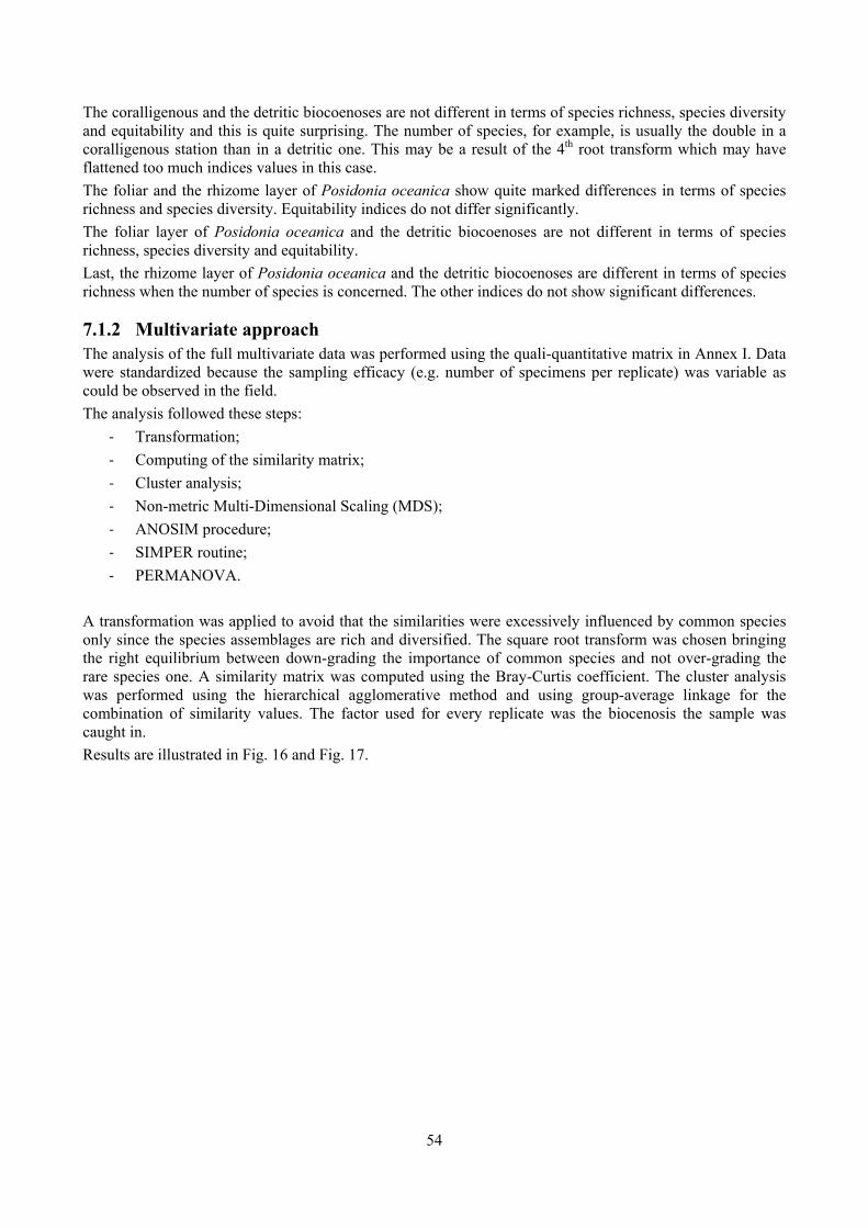
54

The coralligenous and the detritic biocoenoses are not different in terms of species richness, species diversity and equitability and this is quite surprising. The number of species, for example, is usually the double in a coralligenous station than in a detritic one. This may be a result of the 4th root transform which may have flattened too much indices values in this case. The foliar and the rhizome layer of Posidonia oceanica show quite marked differences in terms of species richness and species diversity. Equitability indices do not differ significantly. The foliar layer of Posidonia oceanica and the detritic biocoenoses are not different in terms of species richness, species diversity and equitability. Last, the rhizome layer of Posidonia oceanica and the detritic biocoenoses are different in terms of species richness when the number of species is concerned. The other indices do not show significant differences.

7.1.2 Multivariate approach The analysis of the full multivariate data was performed using the quali-quantitative matrix in Annex I. Data were standardized because the sampling efficacy (e.g. number of specimens per replicate) was variable as could be observed in the field. The analysis followed these steps:

‐ Transformation; ‐ Computing of the similarity matrix; ‐ Cluster analysis; ‐ Non-metric Multi-Dimensional Scaling (MDS); ‐ ANOSIM procedure; ‐ SIMPER routine; ‐ PERMANOVA.

A transformation was applied to avoid that the similarities were excessively influenced by common species only since the species assemblages are rich and diversified. The square root transform was chosen bringing the right equilibrium between down-grading the importance of common species and not over-grading the rare species one. A similarity matrix was computed using the Bray-Curtis coefficient. The cluster analysis was performed using the hierarchical agglomerative method and using group-average linkage for the combination of similarity values. The factor used for every replicate was the biocenosis the sample was caught in. Results are illustrated in Fig. 16 and Fig. 17.

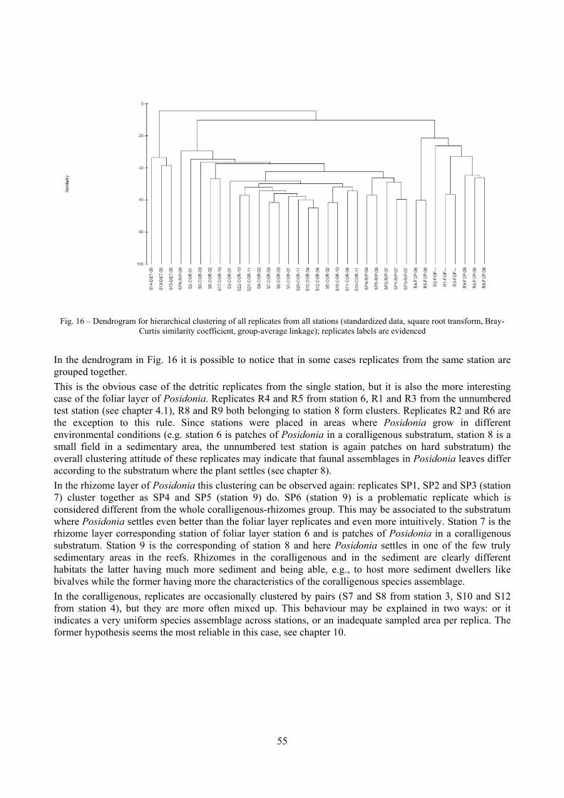
55

Fig. 16 – Dendrogram for hierarchical clustering of all replicates from all stations (standardized data, square root transform, Bray-

Curtis similarity coefficient, group-average linkage); replicates labels are evidenced

In the dendrogram in Fig. 16 it is possible to notice that in some cases replicates from the same station are grouped together. This is the obvious case of the detritic replicates from the single station, but it is also the more interesting case of the foliar layer of Posidonia. Replicates R4 and R5 from station 6, R1 and R3 from the unnumbered test station (see chapter 4.1), R8 and R9 both belonging to station 8 form clusters. Replicates R2 and R6 are the exception to this rule. Since stations were placed in areas where Posidonia grow in different environmental conditions (e.g. station 6 is patches of Posidonia in a coralligenous substratum, station 8 is a small field in a sedimentary area, the unnumbered test station is again patches on hard substratum) the overall clustering attitude of these replicates may indicate that faunal assemblages in Posidonia leaves differ according to the substratum where the plant settles (see chapter 8). In the rhizome layer of Posidonia this clustering can be observed again: replicates SP1, SP2 and SP3 (station 7) cluster together as SP4 and SP5 (station 9) do. SP6 (station 9) is a problematic replicate which is considered different from the whole coralligenous-rhizomes group. This may be associated to the substratum where Posidonia settles even better than the foliar layer replicates and even more intuitively. Station 7 is the rhizome layer corresponding station of foliar layer station 6 and is patches of Posidonia in a coralligenous substratum. Station 9 is the corresponding of station 8 and here Posidonia settles in one of the few truly sedimentary areas in the reefs. Rhizomes in the coralligenous and in the sediment are clearly different habitats the latter having much more sediment and being able, e.g., to host more sediment dwellers like bivalves while the former having more the characteristics of the coralligenous species assemblage. In the coralligenous, replicates are occasionally clustered by pairs (S7 and S8 from station 3, S10 and S12 from station 4), but they are more often mixed up. This behaviour may be explained in two ways: or it indicates a very uniform species assemblage across stations, or an inadequate sampled area per replica. The former hypothesis seems the most reliable in this case, see chapter 10.

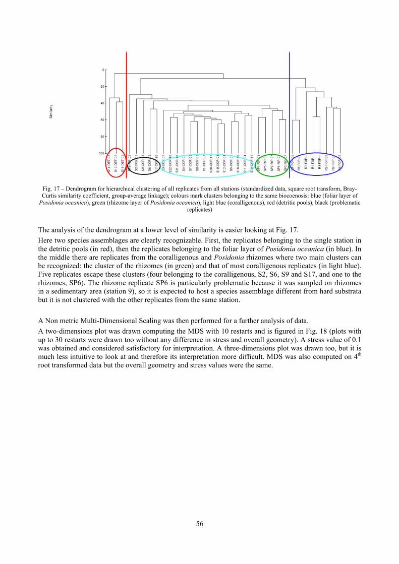
56

Fig. 17 – Dendrogram for hierarchical clustering of all replicates from all stations (standardized data, square root transform, Bray-Curtis similarity coefficient, group-average linkage); colours mark clusters belonging to the same biocoenosis: blue (foliar layer of

Posidonia oceanica), green (rhizome layer of Posidonia oceanica), light blue (coralligenous), red (detritic pools), black (problematic replicates)

The analysis of the dendrogram at a lower level of similarity is easier looking at Fig. 17. Here two species assemblages are clearly recognizable. First, the replicates belonging to the single station in the detritic pools (in red), then the replicates belonging to the foliar layer of Posidonia oceanica (in blue). In the middle there are replicates from the coralligenous and Posidonia rhizomes where two main clusters can be recognized: the cluster of the rhizomes (in green) and that of most coralligenous replicates (in light blue). Five replicates escape these clusters (four belonging to the coralligenous, S2, S6, S9 and S17, and one to the rhizomes, SP6). The rhizome replicate SP6 is particularly problematic because it was sampled on rhizomes in a sedimentary area (station 9), so it is expected to host a species assemblage different from hard substrata but it is not clustered with the other replicates from the same station. A Non metric Multi-Dimensional Scaling was then performed for a further analysis of data. A two-dimensions plot was drawn computing the MDS with 10 restarts and is figured in Fig. 18 (plots with up to 30 restarts were drawn too without any difference in stress and overall geometry). A stress value of 0.1 was obtained and considered satisfactory for interpretation. A three-dimensions plot was drawn too, but it is much less intuitive to look at and therefore its interpretation more difficult. MDS was also computed on 4th root transformed data but the overall geometry and stress values were the same.

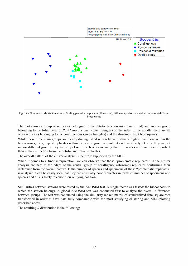
Fig. 18 – Non

The plot shbelonging tother replicWhile thesebiocoenosesin two diffethan in the dThe overall When it coanalysis aredifference fis analysed species and Similarities which the sbetween grotransformeddescribed abThe resultin

n metric Multi-D

hows a groupo the foliar lates belongine three main s, the group erent groups,distinction frpattern of th

omes to a fine here at thefrom the overit can be easthis is likely

between stastation belonoups. The tesd in order tobove. ng R distribut

Dimensional Sc

p of replicatelayer of Posing to the corgroups are c

of replicates, they are verom the detrihe cluster ananer interpretae edges of trall pattern. sily seen thaty to cause the

ations were tengs. A globast was condu

o have data f

tion is the fo

caling plot of al

es belongingidonia ocean

ralligenous (gclearly distin within the c

ery close to eitic and foliaralysis is theration, we cathe central gIf the numbet they are uneir outlying p

ested by the al ANOSIMucted using tfully compa

ollowing:

57

ll replicates (10biocoenoses

g to the detrinica (blue trigreen trianglnguished witcentral groupeach other mr replicates.efore suppor

an observe thgroup of corer of species nusually poorposition.

ANOSIM te test was cothe similarity

arable with th

0 restarts), diffe

itic biocoenoiangles) on tles) and the rth relative dip are not put meaning that

rted by the Mhat those “pralligenous-rand specime

r replicates i

est. A single onducted firsy ranked mathe most sati

erent symbols an

osis (roars inthe sides. In rhizomes (ligistances highaside so cleadifferences

MDS. roblematic r

rhizomes repens of these n terms of n

factor was tst to analysetrix of standaisfying clust

nd colours repr

n red) and anthe middle,

ght blue squaher than thosarly. Despite are much le

replicates” inplicates conf“problemati

number of sp

ested: the bie the overallardized data,ering and M

esent different

nother groupthere are all

ares). se within the

they are putss important

n the clusterfirming theirc replicates”ecimens and

ocoenosis tol differences, square root

MDS-plotting

p l

e t t

r r ” d

o s t g

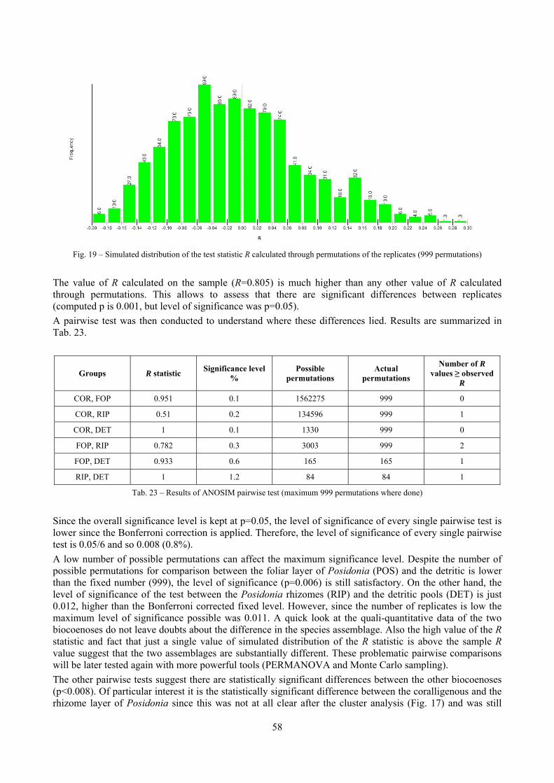
58

Fig. 19 – Simulated distribution of the test statistic R calculated through permutations of the replicates (999 permutations)

The value of R calculated on the sample (R=0.805) is much higher than any other value of R calculated through permutations. This allows to assess that there are significant differences between replicates (computed p is 0.001, but level of significance was p=0.05). A pairwise test was then conducted to understand where these differences lied. Results are summarized in Tab. 23.

Groups R statistic Significance level %

Possible permutations

Actual permutations

Number of R values ≥ observed

R

COR, FOP 0.951 0.1 1562275 999 0

COR, RIP 0.51 0.2 134596 999 1

COR, DET 1 0.1 1330 999 0

FOP, RIP 0.782 0.3 3003 999 2

FOP, DET 0.933 0.6 165 165 1

RIP, DET 1 1.2 84 84 1

Tab. 23 – Results of ANOSIM pairwise test (maximum 999 permutations where done)

Since the overall significance level is kept at p=0.05, the level of significance of every single pairwise test is lower since the Bonferroni correction is applied. Therefore, the level of significance of every single pairwise test is 0.05/6 and so 0.008 (0.8%). A low number of possible permutations can affect the maximum significance level. Despite the number of possible permutations for comparison between the foliar layer of Posidonia (POS) and the detritic is lower than the fixed number (999), the level of significance (p=0.006) is still satisfactory. On the other hand, the level of significance of the test between the Posidonia rhizomes (RIP) and the detritic pools (DET) is just 0.012, higher than the Bonferroni corrected fixed level. However, since the number of replicates is low the maximum level of significance possible was 0.011. A quick look at the quali-quantitative data of the two biocoenoses do not leave doubts about the difference in the species assemblage. Also the high value of the R statistic and fact that just a single value of simulated distribution of the R statistic is above the sample R value suggest that the two assemblages are substantially different. These problematic pairwise comparisons will be later tested again with more powerful tools (PERMANOVA and Monte Carlo sampling). The other pairwise tests suggest there are statistically significant differences between the other biocoenoses (p<0.008). Of particular interest it is the statistically significant difference between the coralligenous and the rhizome layer of Posidonia since this was not at all clear after the cluster analysis (Fig. 17) and was still

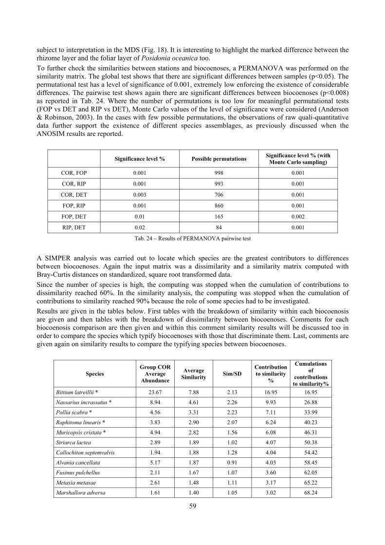
59

subject to interpretation in the MDS (Fig. 18). It is interesting to highlight the marked difference between the rhizome layer and the foliar layer of Posidonia oceanica too. To further check the similarities between stations and biocoenoses, a PERMANOVA was performed on the similarity matrix. The global test shows that there are significant differences between samples (p<0.05). The permutational test has a level of significance of 0.001, extremely low enforcing the existence of considerable differences. The pairwise test shows again there are significant differences between biocoenoses (p<0.008) as reported in Tab. 24. Where the number of permutations is too low for meaningful permutational tests (FOP vs DET and RIP vs DET), Monte Carlo values of the level of significance were considered (Anderson & Robinson, 2003). In the cases with few possible permutations, the observations of raw quali-quantitative data further support the existence of different species assemblages, as previously discussed when the ANOSIM results are reported.

Significance level % Possible permutations Significance level % (with Monte Carlo sampling)

COR, FOP 0.001 998 0.001

COR, RIP 0.001 993 0.001

COR, DET 0.003 706 0.001

FOP, RIP 0.001 860 0.001

FOP, DET 0.01 165 0.002

RIP, DET 0.02 84 0.001

Tab. 24 – Results of PERMANOVA pairwise test

A SIMPER analysis was carried out to locate which species are the greatest contributors to differences between biocoenoses. Again the input matrix was a dissimilarity and a similarity matrix computed with Bray-Curtis distances on standardized, square root transformed data. Since the number of species is high, the computing was stopped when the cumulation of contributions to dissimilarity reached 60%. In the similarity analysis, the computing was stopped when the cumulation of contributions to similarity reached 90% because the role of some species had to be investigated. Results are given in the tables below. First tables with the breakdown of similarity within each biocoenosis are given and then tables with the breakdown of dissimilarity between biocoenoses. Comments for each biocoenosis comparison are then given and within this comment similarity results will be discussed too in order to compare the species which typify biocoenoses with those that discriminate them. Last, comments are given again on similarity results to compare the typifying species between biocoenoses.

Species Group COR

Average Abundance

Average Similarity Sim/SD

Contribution to similarity

%

Cumulations of

contributions to similarity%

Bittium latreillii * 23.67 7.88 2.13 16.95 16.95

Nassarius incrassatus * 8.94 4.61 2.26 9.93 26.88

Pollia scabra * 4.56 3.31 2.23 7.11 33.99

Raphitoma linearis * 3.83 2.90 2.07 6.24 40.23

Muricopsis cristata * 4.94 2.82 1.56 6.08 46.31

Striarca lactea 2.89 1.89 1.02 4.07 50.38

Callochiton septemvalvis 1.94 1.88 1.28 4.04 54.42

Alvania cancellata 5.17 1.87 0.91 4.03 58.45

Fusinus pulchellus 2.11 1.67 1.07 3.60 62.05

Metaxia metaxae 2.61 1.48 1.11 3.17 65.22

Marshallora adversa 1.61 1.40 1.05 3.02 68.24

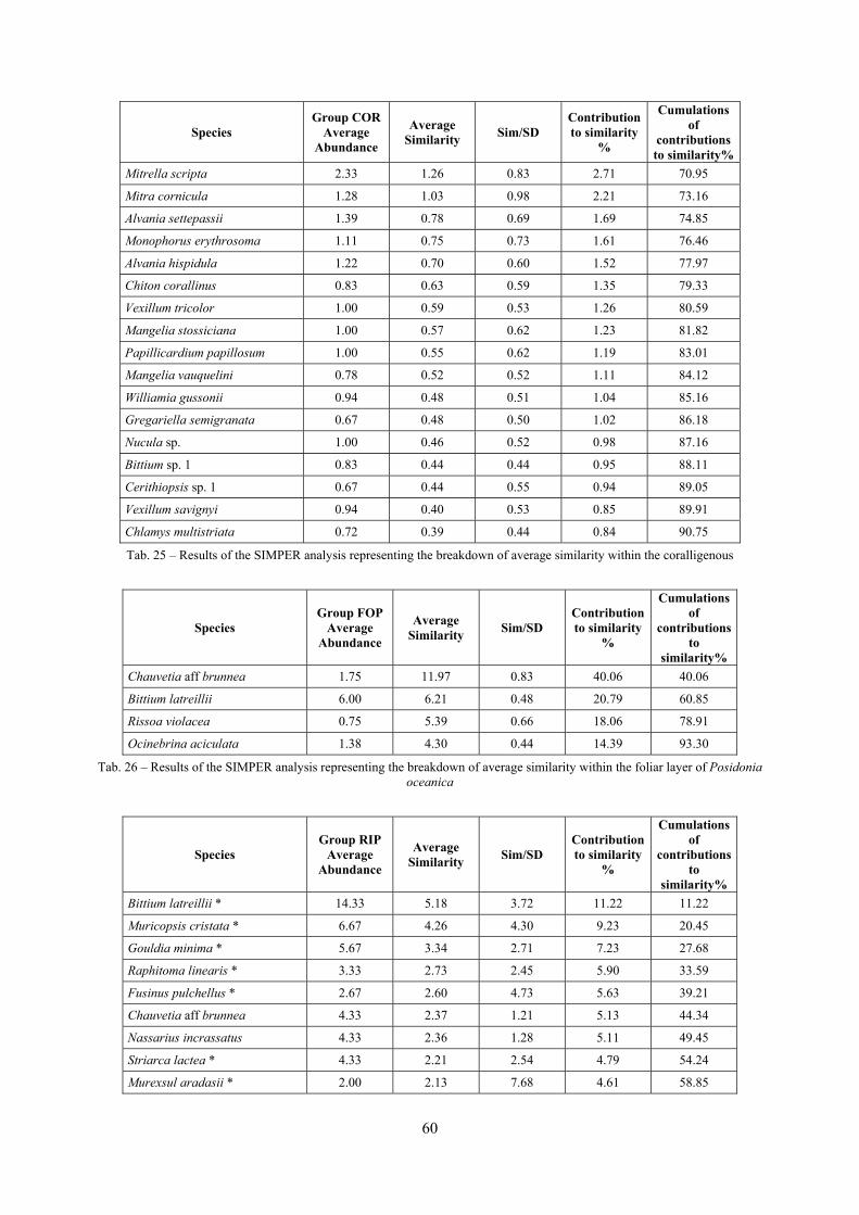
60

Species Group COR

Average Abundance

Average Similarity Sim/SD

Contribution to similarity

%

Cumulations of

contributions to similarity%

Mitrella scripta 2.33 1.26 0.83 2.71 70.95

Mitra cornicula 1.28 1.03 0.98 2.21 73.16

Alvania settepassii 1.39 0.78 0.69 1.69 74.85

Monophorus erythrosoma 1.11 0.75 0.73 1.61 76.46

Alvania hispidula 1.22 0.70 0.60 1.52 77.97

Chiton corallinus 0.83 0.63 0.59 1.35 79.33

Vexillum tricolor 1.00 0.59 0.53 1.26 80.59

Mangelia stossiciana 1.00 0.57 0.62 1.23 81.82

Papillicardium papillosum 1.00 0.55 0.62 1.19 83.01

Mangelia vauquelini 0.78 0.52 0.52 1.11 84.12

Williamia gussonii 0.94 0.48 0.51 1.04 85.16

Gregariella semigranata 0.67 0.48 0.50 1.02 86.18

Nucula sp. 1.00 0.46 0.52 0.98 87.16

Bittium sp. 1 0.83 0.44 0.44 0.95 88.11

Cerithiopsis sp. 1 0.67 0.44 0.55 0.94 89.05

Vexillum savignyi 0.94 0.40 0.53 0.85 89.91

Chlamys multistriata 0.72 0.39 0.44 0.84 90.75

Tab. 25 – Results of the SIMPER analysis representing the breakdown of average similarity within the coralligenous

Species Group FOP

Average Abundance

Average Similarity Sim/SD

Contribution to similarity

%

Cumulations of

contributions to

similarity% Chauvetia aff brunnea 1.75 11.97 0.83 40.06 40.06

Bittium latreillii 6.00 6.21 0.48 20.79 60.85

Rissoa violacea 0.75 5.39 0.66 18.06 78.91

Ocinebrina aciculata 1.38 4.30 0.44 14.39 93.30

Tab. 26 – Results of the SIMPER analysis representing the breakdown of average similarity within the foliar layer of Posidonia oceanica

Species Group RIP

Average Abundance

Average Similarity Sim/SD

Contribution to similarity

%

Cumulations of

contributions to

similarity% Bittium latreillii * 14.33 5.18 3.72 11.22 11.22

Muricopsis cristata * 6.67 4.26 4.30 9.23 20.45

Gouldia minima * 5.67 3.34 2.71 7.23 27.68

Raphitoma linearis * 3.33 2.73 2.45 5.90 33.59

Fusinus pulchellus * 2.67 2.60 4.73 5.63 39.21

Chauvetia aff brunnea 4.33 2.37 1.21 5.13 44.34

Nassarius incrassatus 4.33 2.36 1.28 5.11 49.45

Striarca lactea * 4.33 2.21 2.54 4.79 54.24

Murexsul aradasii * 2.00 2.13 7.68 4.61 58.85

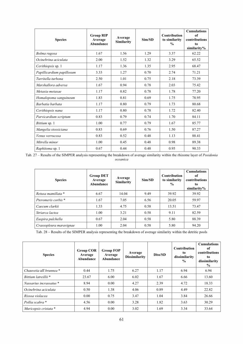
61

Species Group RIP

Average Abundance

Average Similarity Sim/SD

Contribution to similarity

%

Cumulations of

contributions to

similarity% Bolma rugosa 1.67 1.56 1.29 3.37 62.22

Ocinebrina aciculata 2.00 1.52 1.32 3.29 65.52

Cerithiopsis sp. 1 1.17 1.36 1.35 2.95 68.47

Papillicardium papillosum 3.33 1.27 0.70 2.74 71.21

Turritella turbona 2.50 1.01 0.75 2.18 73.39

Marshallora adversa 1.67 0.94 0.78 2.03 75.42

Metaxia metaxae 1.17 0.82 0.78 1.78 77.20

Homalopoma sanguineum 1.83 0.81 0.69 1.75 78.95

Barbatia barbata 1.17 0.80 0.79 1.73 80.68

Cerithiopsis nana 1.17 0.80 0.78 1.72 82.40

Parvicardium scriptum 0.83 0.79 0.74 1.70 84.11

Bittium sp. 1 1.00 0.77 0.79 1.67 85.77

Mangelia stossiciana 0.83 0.69 0.76 1.50 87.27

Venus verrucosa 0.83 0.52 0.48 1.13 88.41

Mitrella minor 1.00 0.45 0.48 0.98 89.38

Raphitoma sp. 1 0.67 0.44 0.48 0.95 90.33

Tab. 27 – Results of the SIMPER analysis representing the breakdown of average similarity within the rhizome layer of Posidonia oceanica

Species Group DET

Average Abundance

Average Similarity Sim/SD

Contribution to similarity

%

Cumulations of

contributions to

similarity% Retusa mamillata * 6.67 14.04 9.49 39.92 39.92

Pteromeris corbis * 1.67 7.05 6.56 20.05 59.97

Caecum clarkii 1.33 4.75 0.58 13.51 73.47

Striarca lactea 1.00 3.21 0.58 9.11 82.59

Euspira pulchella 0.67 2.04 0.58 5.80 88.39

Crassopleura maravignae 1.00 2.04 0.58 5.80 94.20

Tab. 28 – Results of the SIMPER analysis representing the breakdown of average similarity within the detritic pools

Species Group COR

Average Abundance

Group FOP Average

Abundance

Average Dissimilarity Diss/SD

Contribution to

dissimilarity %

Cumulations of

contributions to

dissimilarity%

Chauvetia aff brunnea * 0.44 1.75 6.27 1.17 6.94 6.94

Bittium latreillii * 23.67 6.00 6.02 1.67 6.66 13.60

Nassarius incrassatus * 8.94 0.00 4.27 2.39 4.72 18.33

Ocinebrina aciculata 0.50 1.38 4.06 0.89 4.49 22.82

Rissoa violacea 0.00 0.75 3.47 1.04 3.84 26.66

Pollia scabra * 4.56 0.00 3.28 1.82 3.63 30.29

Muricopsis cristata * 4.94 0.00 3.02 1.69 3.34 33.64

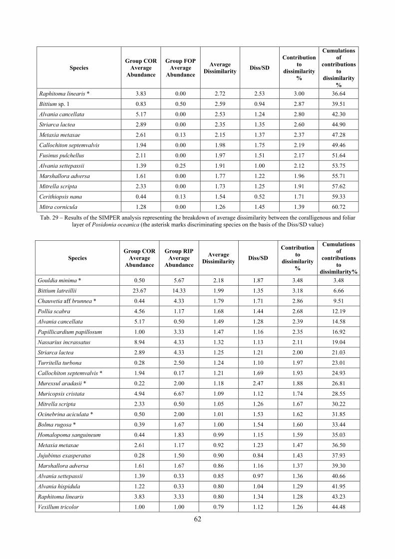
62

Species Group COR

Average Abundance

Group FOP Average

Abundance

Average Dissimilarity Diss/SD

Contribution to

dissimilarity %

Cumulations of

contributions to

dissimilarity%

Raphitoma linearis * 3.83 0.00 2.72 2.53 3.00 36.64

Bittium sp. 1 0.83 0.50 2.59 0.94 2.87 39.51

Alvania cancellata 5.17 0.00 2.53 1.24 2.80 42.30

Striarca lactea 2.89 0.00 2.35 1.35 2.60 44.90

Metaxia metaxae 2.61 0.13 2.15 1.37 2.37 47.28

Callochiton septemvalvis 1.94 0.00 1.98 1.75 2.19 49.46

Fusinus pulchellus 2.11 0.00 1.97 1.51 2.17 51.64

Alvania settepassii 1.39 0.25 1.91 1.00 2.12 53.75

Marshallora adversa 1.61 0.00 1.77 1.22 1.96 55.71

Mitrella scripta 2.33 0.00 1.73 1.25 1.91 57.62

Cerithiopsis nana 0.44 0.13 1.54 0.52 1.71 59.33

Mitra cornicula 1.28 0.00 1.26 1.45 1.39 60.72

Tab. 29 – Results of the SIMPER analysis representing the breakdown of average dissimilarity between the coralligenous and foliar layer of Posidonia oceanica (the asterisk marks discriminating species on the basis of the Diss/SD value)

Species Group COR

Average Abundance

Group RIP Average

Abundance

Average Dissimilarity Diss/SD

Contribution to

dissimilarity %

Cumulations of

contributions to

dissimilarity%Gouldia minima * 0.50 5.67 2.18 1.87 3.48 3.48

Bittium latreillii 23.67 14.33 1.99 1.35 3.18 6.66

Chauvetia aff brunnea * 0.44 4.33 1.79 1.71 2.86 9.51

Pollia scabra 4.56 1.17 1.68 1.44 2.68 12.19

Alvania cancellata 5.17 0.50 1.49 1.28 2.39 14.58

Papillicardium papillosum 1.00 3.33 1.47 1.16 2.35 16.92

Nassarius incrassatus 8.94 4.33 1.32 1.13 2.11 19.04

Striarca lactea 2.89 4.33 1.25 1.21 2.00 21.03

Turritella turbona 0.28 2.50 1.24 1.10 1.97 23.01

Callochiton septemvalvis * 1.94 0.17 1.21 1.69 1.93 24.93

Murexsul aradasii * 0.22 2.00 1.18 2.47 1.88 26.81

Muricopsis cristata 4.94 6.67 1.09 1.12 1.74 28.55

Mitrella scripta 2.33 0.50 1.05 1.26 1.67 30.22

Ocinebrina aciculata * 0.50 2.00 1.01 1.53 1.62 31.85

Bolma rugosa * 0.39 1.67 1.00 1.54 1.60 33.44

Homalopoma sanguineum 0.44 1.83 0.99 1.15 1.59 35.03

Metaxia metaxae 2.61 1.17 0.92 1.23 1.47 36.50

Jujubinus exasperatus 0.28 1.50 0.90 0.84 1.43 37.93

Marshallora adversa 1.61 1.67 0.86 1.16 1.37 39.30

Alvania settepassii 1.39 0.33 0.85 0.97 1.36 40.66

Alvania hispidula 1.22 0.33 0.80 1.04 1.29 41.95

Raphitoma linearis 3.83 3.33 0.80 1.34 1.28 43.23

Vexillum tricolor 1.00 1.00 0.79 1.12 1.26 44.48

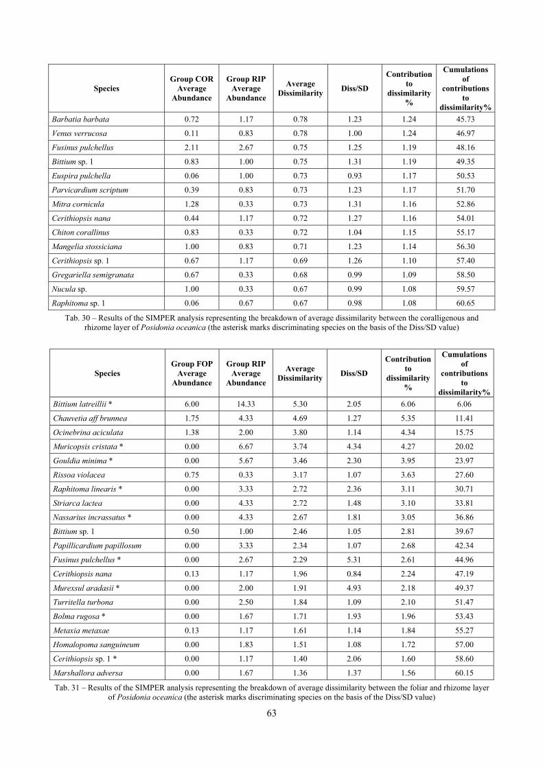
63

Species Group COR

Average Abundance

Group RIP Average

Abundance

Average Dissimilarity Diss/SD

Contribution to

dissimilarity %

Cumulations of

contributions to

dissimilarity%Barbatia barbata 0.72 1.17 0.78 1.23 1.24 45.73

Venus verrucosa 0.11 0.83 0.78 1.00 1.24 46.97

Fusinus pulchellus 2.11 2.67 0.75 1.25 1.19 48.16

Bittium sp. 1 0.83 1.00 0.75 1.31 1.19 49.35

Euspira pulchella 0.06 1.00 0.73 0.93 1.17 50.53

Parvicardium scriptum 0.39 0.83 0.73 1.23 1.17 51.70

Mitra cornicula 1.28 0.33 0.73 1.31 1.16 52.86

Cerithiopsis nana 0.44 1.17 0.72 1.27 1.16 54.01

Chiton corallinus 0.83 0.33 0.72 1.04 1.15 55.17

Mangelia stossiciana 1.00 0.83 0.71 1.23 1.14 56.30

Cerithiopsis sp. 1 0.67 1.17 0.69 1.26 1.10 57.40

Gregariella semigranata 0.67 0.33 0.68 0.99 1.09 58.50

Nucula sp. 1.00 0.33 0.67 0.99 1.08 59.57

Raphitoma sp. 1 0.06 0.67 0.67 0.98 1.08 60.65

Tab. 30 – Results of the SIMPER analysis representing the breakdown of average dissimilarity between the coralligenous and rhizome layer of Posidonia oceanica (the asterisk marks discriminating species on the basis of the Diss/SD value)

Species Group FOP

Average Abundance

Group RIP Average

Abundance

Average Dissimilarity Diss/SD

Contribution to

dissimilarity %

Cumulations of

contributions to

dissimilarity%Bittium latreillii * 6.00 14.33 5.30 2.05 6.06 6.06

Chauvetia aff brunnea 1.75 4.33 4.69 1.27 5.35 11.41

Ocinebrina aciculata 1.38 2.00 3.80 1.14 4.34 15.75

Muricopsis cristata * 0.00 6.67 3.74 4.34 4.27 20.02

Gouldia minima * 0.00 5.67 3.46 2.30 3.95 23.97

Rissoa violacea 0.75 0.33 3.17 1.07 3.63 27.60

Raphitoma linearis * 0.00 3.33 2.72 2.36 3.11 30.71

Striarca lactea 0.00 4.33 2.72 1.48 3.10 33.81

Nassarius incrassatus * 0.00 4.33 2.67 1.81 3.05 36.86

Bittium sp. 1 0.50 1.00 2.46 1.05 2.81 39.67

Papillicardium papillosum 0.00 3.33 2.34 1.07 2.68 42.34

Fusinus pulchellus * 0.00 2.67 2.29 5.31 2.61 44.96

Cerithiopsis nana 0.13 1.17 1.96 0.84 2.24 47.19

Murexsul aradasii * 0.00 2.00 1.91 4.93 2.18 49.37

Turritella turbona 0.00 2.50 1.84 1.09 2.10 51.47

Bolma rugosa * 0.00 1.67 1.71 1.93 1.96 53.43

Metaxia metaxae 0.13 1.17 1.61 1.14 1.84 55.27

Homalopoma sanguineum 0.00 1.83 1.51 1.08 1.72 57.00

Cerithiopsis sp. 1 * 0.00 1.17 1.40 2.06 1.60 58.60

Marshallora adversa 0.00 1.67 1.36 1.37 1.56 60.15

Tab. 31 – Results of the SIMPER analysis representing the breakdown of average dissimilarity between the foliar and rhizome layer of Posidonia oceanica (the asterisk marks discriminating species on the basis of the Diss/SD value)

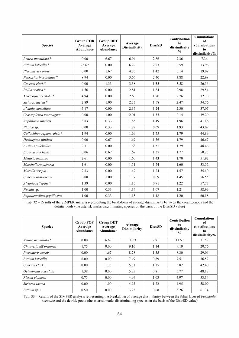
64

Species Group COR

Average Abundance

Group DET Average

Abundance

Average Dissimilarity Diss/SD

Contribution to

dissimilarity %

Cumulations of

contributions to

dissimilarity%Retusa mamillata * 0.00 6.67 6.94 2.86 7.36 7.36

Bittium latreillii * 23.67 0.00 6.22 2.23 6.59 13.96

Pteromeris corbis 0.00 1.67 4.85 1.42 5.14 19.09

Nassarius incrassatus * 8.94 0.00 3.66 2.40 3.88 22.98

Caecum clarkii 0.00 1.33 3.38 1.35 3.58 26.56

Pollia scabra * 4.56 0.00 2.81 1.84 2.98 29.54

Muricopsis cristata * 4.94 0.00 2.60 1.70 2.76 32.30

Striarca lactea * 2.89 1.00 2.33 1.58 2.47 34.76

Alvania cancellata 5.17 0.00 2.17 1.24 2.30 37.07

Crassopleura maravignae 0.00 1.00 2.01 1.35 2.14 39.20

Raphitoma linearis 3.83 0.33 1.85 1.49 1.96 41.16

Philine sp. 0.00 0.33 1.82 0.69 1.93 43.09

Callochiton septemvalvis * 1.94 0.00 1.69 1.75 1.79 44.89

Hemilepton nitidum 0.00 0.67 1.69 1.36 1.79 46.67

Fusinus pulchellus 2.11 0.00 1.68 1.51 1.79 48.46

Euspira pulchella 0.06 0.67 1.67 1.37 1.77 50.23

Metaxia metaxae 2.61 0.00 1.60 1.43 1.70 51.92

Marshallora adversa 1.61 0.00 1.51 1.24 1.60 53.52

Mitrella scripta 2.33 0.00 1.49 1.24 1.57 55.10

Caecum armoricum 0.00 1.00 1.37 0.69 1.45 56.55

Alvania settepassii 1.39 0.00 1.15 0.91 1.22 57.77

Nucula sp. 1.00 0.33 1.14 1.07 1.21 58.99

Papillicardium papillosum 1.00 0.33 1.13 1.18 1.20 60.18

Tab. 32 – Results of the SIMPER analysis representing the breakdown of average dissimilarity between the coralligenous and the detritic pools (the asterisk marks discriminating species on the basis of the Diss/SD value)

Species Group FOP

Average Abundance

Group DET Average

Abundance

Average Dissimilarity Diss/SD

Contribution to

dissimilarity %

Cumulations of

contributions to

dissimilarity%Retusa mamillata * 0.00 6.67 11.53 2.91 11.57 11.57

Chauvetia aff brunnea 1.75 0.00 9.16 1.14 9.19 20.76

Pteromeris corbis 0.00 1.67 8.28 1.35 8.30 29.06

Bittium latreillii 6.00 0.00 7.49 0.89 7.51 36.57

Caecum clarkii 0.00 1.33 5.81 1.35 5.82 42.40

Ocinebrina aciculata 1.38 0.00 5.75 0.81 5.77 48.17

Rissoa violacea 0.75 0.00 4.96 1.03 4.97 53.14

Striarca lactea 0.00 1.00 4.93 1.22 4.95 58.09

Bittium sp. 1 0.50 0.00 3.25 0.68 3.26 61.34

Tab. 33 – Results of the SIMPER analysis representing the breakdown of average dissimilarity between the foliar layer of Posidonia oceanica and the detritic pools (the asterisk marks discriminating species on the basis of the Diss/SD value)

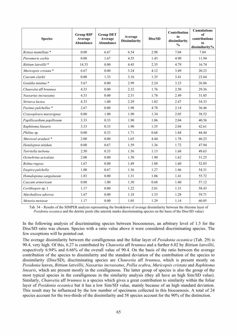
65

Species Group RIP

Average Abundance

Group DET Average

Abundance

Average Dissimilarity Diss/SD

Contribution to

dissimilarity %

Cumulations of

contributions to

dissimilarity%Retusa mamillata * 0.00 6.67 6.54 2.98 7.04 7.04

Pteromeris corbis 0.00 1.67 4.55 1.43 4.90 11.94

Bittium latreillii * 14.33 0.00 4.45 2.35 4.79 16.74

Muricopsis cristata * 6.67 0.00 3.24 4.12 3.49 20.23

Caecum clarkii 0.00 1.33 3.16 1.35 3.41 23.64

Gouldia minima * 5.67 0.00 2.99 2.24 3.23 26.86

Chauvetia aff brunnea 4.33 0.00 2.32 1.76 2.50 29.36

Nassarius incrassatus 4.33 0.00 2.31 1.78 2.49 31.85

Striarca lactea 4.33 1.00 2.29 1.82 2.47 34.33

Fusinus pulchellus * 2.67 0.00 1.98 4.78 2.14 36.46

Crassopleura maravignae 0.00 1.00 1.90 1.34 2.05 38.52

Papillicardium papillosum 3.33 0.33 1.90 1.06 2.04 40.56

Raphitoma linearis 3.33 0.33 1.90 1.55 2.04 42.61

Philine sp. 0.00 0.33 1.71 0.68 1.84 44.44

Murexsul aradasii * 2.00 0.00 1.65 4.44 1.78 46.23

Hemilepton nitidum 0.00 0.67 1.59 1.36 1.72 47.94

Turritella turbona 2.50 0.33 1.56 1.13 1.68 49.63

Ocinebrina aciculata 2.00 0.00 1.50 1.90 1.62 51.25

Bolma rugosa 1.67 0.00 1.49 1.88 1.60 52.85

Euspira pulchella 1.00 0.67 1.36 1.27 1.46 54.31

Homalopoma sanguineum 1.83 0.00 1.31 1.06 1.41 55.72

Caecum armoricum 0.00 1.00 1.30 0.68 1.40 57.12

Cerithiopsis sp. 1 1.17 0.00 1.22 2.01 1.31 58.43

Marshallora adversa 1.67 0.00 1.18 1.33 1.28 59.71

Metaxia metaxae 1.17 0.00 1.05 1.29 1.14 60.85

Tab. 34 – Results of the SIMPER analysis representing the breakdown of average dissimilarity between the rhizome layer of Posidonia oceanica and the detritic pools (the asterisk marks discriminating species on the basis of the Diss/SD value)

In the following analysis of discriminating species between biocoenoses, an arbitrary level of 1.5 for the Diss/SD ratio was chosen. Species with a ratio value above it were considered discriminating species. The few exceptions will be pointed out. The average dissimilarity between the coralligenous and the foliar layer of Posidonia oceanica (Tab. 29) is 90.4, very high. Of this, 6.27 is contributed by Chauvetia aff brunnea and a further 6.02 by Bittium latreillii, respectively 6.94% and 6.66% of the overall value of 90.4. On the basis of the ratio between the average contribution of the species to dissimilarity and the standard deviation of the contribution of the species to dissimilarity (Diss/SD), discriminating species are Chauvetia aff brunnea, which is present mostly on Posidonia leaves, Bittium latreillii, Nassarius incrassatus, Pollia scabra, Muricopsis cristata and Raphitoma linearis, which are present mostly in the coralligenous. The latter group of species is also the group of the most typical species in the coralligenous in the similarity analysis (they all have an high Sim/SD value). Similarly, Chauvetia aff brunnea is a species which gives a great contribution to similarity within the foliar layer of Posidonia oceanica but it has a low Sim/SD value, mainly because of an high standard deviation. This result may be influenced by the low number of specimens collected in this biocoenosis. A total of 24 species account for the two-thirds of the dissimilarity and 58 species account for the 90% of the distinction.

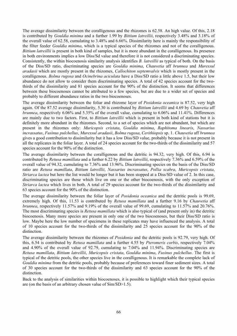
66

The average dissimilarity between the coralligenous and the rhizomes is 62.58. An high value. Of this, 2.18 is contributed by Gouldia minima and a further 1.99 by Bittium latreillii, respectively 3.48% and 3.18% of the overall value of 62.58, cumulating to 3.48% and 6.66%. Dissimilarity here is mainly the responsibility of the filter feeder Gouldia minima, which is a typical species of the rhizomes and not of the coralligenous. Bittium latreillii is present in both kind of samples, but it is more abundant in the coralligenous. Its presence in both environments implies a low Diss/Sd value and therefore it is not considered a discriminating species. Consistently, the within biocoenosis similarity analysis identifies B. latreillii as typical of both. On the basis of the Diss/SD ratio, discriminating species are Gouldia minima, Chauvetia aff brunnea and Murexsul aradasii which are mostly present in the rhizomes, Callochiton septemvalvis which is mostly present in the coralligenous. Bolma rugosa and Ocinebrina aciculata have a Diss/SD ratio a little above 1.5, but their low abundance do not allow to consider them discriminating species. A total of 42 species account for the two-thirds of the dissimilarity and 81 species account for the 90% of the distinction. It seems that differences between these biocoenoses cannot be attributed to a few species, but are due to a wider set of species and probably to different abundance ratios in the two biocoenoses. The average dissimilarity between the foliar and rhizome layer of Posidonia oceanica is 87.52, very high again. Of the 87.52 average dissimilarity, 5.30 is contributed by Bittium latreillii and 4.69 by Chauvetia aff brunnea, respectively 6.06% and 5.35% of the overall value, cumulating to 6.06% and 11.41%. Differences are mainly due to two factors. First, to Bittium latreillii which is present in both kind of stations but it is definitely more abundant in the rhizomes. Second, to a set of species which are not abundant, but which are present in the rhizomes only: Muricopsis cristata, Gouldia minima, Raphitoma linearis, Nassarius incrassatus, Fusinus pulchellus, Murexsul aradasii, Bolma rugosa, Cerithiopsis sp. 1. Chauvetia aff brunnea gives a good contribution to dissimilarity but it has a low Diss/SD value, probably because it is not present in all the replicates in the foliar layer. A total of 24 species account for the two-thirds of the dissimilarity and 57 species account for the 90% of the distinction. The average dissimilarity between the coralligenous and the detritic is 94.32, very high. Of this, 6.94 is contributed by Retusa mamillata and a further 6.22 by Bittium latreillii, respectively 7.36% and 6.59% of the overall value of 94.32, cumulating to 7.36% and 13.96%. Discriminating species on the basis of the Diss/SD ratio are Retusa mamillata, Bittium latreillii, Nassarius incrassatus, Pollia scabra, Muricopsis cristata, Striarca lactea but here the list would be longer but it has been stopped at a Diss/SD value of 2. In this case, discriminating species are those which live on one or the other biocoenosis, with the only exception of Striarca lactea which lives in both. A total of 29 species account for the two-thirds of the dissimilarity and 63 species account for the 90% of the distinction. The average dissimilarity between the foliar layer of Posidonia oceanica and the detritic pools is 99.69, extremely high. Of this, 11.53 is contributed by Retusa mamillata and a further 9.16 by Chauvetia aff brunnea, respectively 11.57% and 9.19% of the overall value of 99.69, cumulating to 11.57% and 20.76%. The most discriminating species is Retusa mamillata which is also typical of (and present only in) the detritic biocoenosis. Many more species are present in only one of the two biocoenoses, but their Diss/SD ratio is low. Maybe here the low number of specimens in these replicates may have influenced the analysis. A total of 10 species account for the two-thirds of the dissimilarity and 25 species account for the 90% of the distinction. The average dissimilarity between the rhizomes of Posidonia and the detritic pools is 92.79, very high. Of this, 6.54 is contributed by Retusa mamillata and a further 4.55 by Pteromeris corbis, respectively 7.04% and 4.90% of the overall value of 92.79, cumulating to 7.04% and 11.94%. Discriminating species are Retusa mamillata, Bittium latreillii, Muricopsis cristata, Gouldia minima, Fusinus pulchellus. The first is typical of the detritic pools, the other species live in the coralligenous. It is remarkable the complete lack of Gouldia minima from the detritic pools, probably because of preferences toward finer sediment sizes. A total of 30 species account for the two-thirds of the dissimilarity and 63 species account for the 90% of the distinction. Back to the analysis of similarities within biocoenoses, it is possible to highlight which their typical species are (on the basis of an arbitrary chosen value of Sim/SD>1.5).

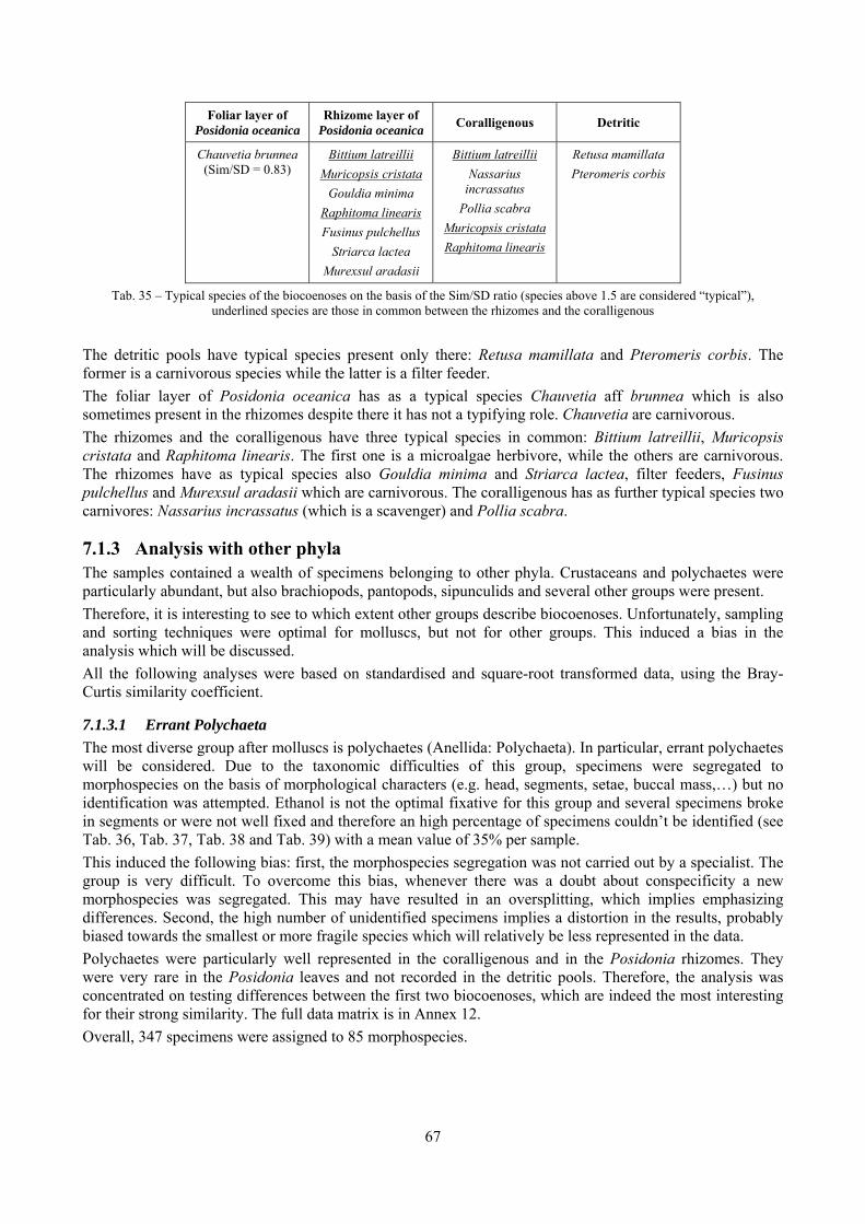
67

Foliar layer of Posidonia oceanica

Rhizome layer of Posidonia oceanica Coralligenous Detritic

Chauvetia brunnea (Sim/SD = 0.83)

Bittium latreillii Muricopsis cristata

Gouldia minima Raphitoma linearis Fusinus pulchellus

Striarca lactea Murexsul aradasii

Bittium latreillii Nassarius

incrassatus Pollia scabra

Muricopsis cristata Raphitoma linearis

Retusa mamillata Pteromeris corbis

Tab. 35 – Typical species of the biocoenoses on the basis of the Sim/SD ratio (species above 1.5 are considered “typical”), underlined species are those in common between the rhizomes and the coralligenous

The detritic pools have typical species present only there: Retusa mamillata and Pteromeris corbis. The former is a carnivorous species while the latter is a filter feeder. The foliar layer of Posidonia oceanica has as a typical species Chauvetia aff brunnea which is also sometimes present in the rhizomes despite there it has not a typifying role. Chauvetia are carnivorous. The rhizomes and the coralligenous have three typical species in common: Bittium latreillii, Muricopsis cristata and Raphitoma linearis. The first one is a microalgae herbivore, while the others are carnivorous. The rhizomes have as typical species also Gouldia minima and Striarca lactea, filter feeders, Fusinus pulchellus and Murexsul aradasii which are carnivorous. The coralligenous has as further typical species two carnivores: Nassarius incrassatus (which is a scavenger) and Pollia scabra.

7.1.3 Analysis with other phyla The samples contained a wealth of specimens belonging to other phyla. Crustaceans and polychaetes were particularly abundant, but also brachiopods, pantopods, sipunculids and several other groups were present. Therefore, it is interesting to see to which extent other groups describe biocoenoses. Unfortunately, sampling and sorting techniques were optimal for molluscs, but not for other groups. This induced a bias in the analysis which will be discussed. All the following analyses were based on standardised and square-root transformed data, using the Bray-Curtis similarity coefficient.

7.1.3.1 Errant Polychaeta The most diverse group after molluscs is polychaetes (Anellida: Polychaeta). In particular, errant polychaetes will be considered. Due to the taxonomic difficulties of this group, specimens were segregated to morphospecies on the basis of morphological characters (e.g. head, segments, setae, buccal mass,…) but no identification was attempted. Ethanol is not the optimal fixative for this group and several specimens broke in segments or were not well fixed and therefore an high percentage of specimens couldn’t be identified (see Tab. 36, Tab. 37, Tab. 38 and Tab. 39) with a mean value of 35% per sample. This induced the following bias: first, the morphospecies segregation was not carried out by a specialist. The group is very difficult. To overcome this bias, whenever there was a doubt about conspecificity a new morphospecies was segregated. This may have resulted in an oversplitting, which implies emphasizing differences. Second, the high number of unidentified specimens implies a distortion in the results, probably biased towards the smallest or more fragile species which will relatively be less represented in the data. Polychaetes were particularly well represented in the coralligenous and in the Posidonia rhizomes. They were very rare in the Posidonia leaves and not recorded in the detritic pools. Therefore, the analysis was concentrated on testing differences between the first two biocoenoses, which are indeed the most interesting for their strong similarity. The full data matrix is in Annex 12. Overall, 347 specimens were assigned to 85 morphospecies.

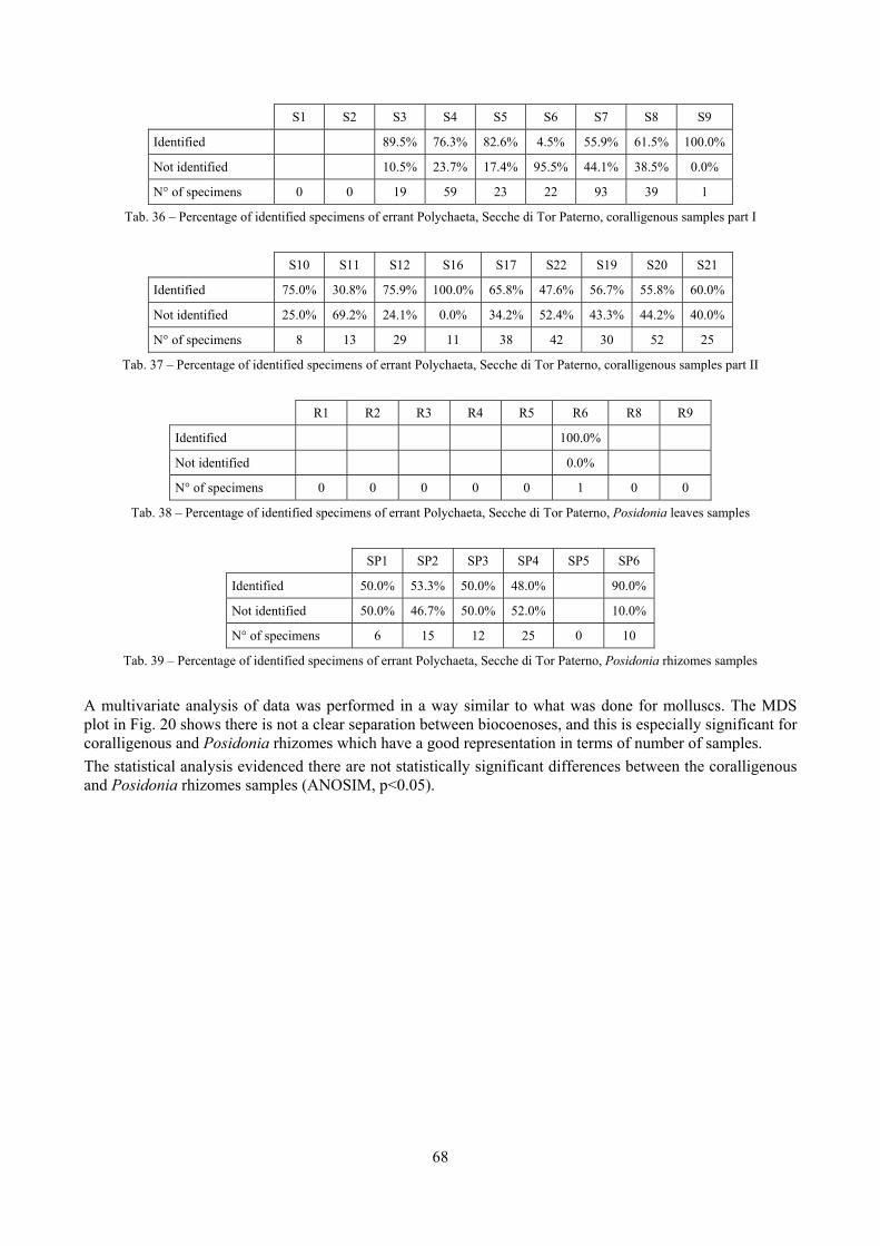
68

S1 S2 S3 S4 S5 S6 S7 S8 S9

Identified 89.5% 76.3% 82.6% 4.5% 55.9% 61.5% 100.0%

Not identified 10.5% 23.7% 17.4% 95.5% 44.1% 38.5% 0.0%

N° of specimens 0 0 19 59 23 22 93 39 1

Tab. 36 – Percentage of identified specimens of errant Polychaeta, Secche di Tor Paterno, coralligenous samples part I

S10 S11 S12 S16 S17 S22 S19 S20 S21

Identified 75.0% 30.8% 75.9% 100.0% 65.8% 47.6% 56.7% 55.8% 60.0%

Not identified 25.0% 69.2% 24.1% 0.0% 34.2% 52.4% 43.3% 44.2% 40.0%

N° of specimens 8 13 29 11 38 42 30 52 25

Tab. 37 – Percentage of identified specimens of errant Polychaeta, Secche di Tor Paterno, coralligenous samples part II

R1 R2 R3 R4 R5 R6 R8 R9

Identified 100.0%

Not identified 0.0%

N° of specimens 0 0 0 0 0 1 0 0

Tab. 38 – Percentage of identified specimens of errant Polychaeta, Secche di Tor Paterno, Posidonia leaves samples

SP1 SP2 SP3 SP4 SP5 SP6

Identified 50.0% 53.3% 50.0% 48.0% 90.0%

Not identified 50.0% 46.7% 50.0% 52.0% 10.0%

N° of specimens 6 15 12 25 0 10

Tab. 39 – Percentage of identified specimens of errant Polychaeta, Secche di Tor Paterno, Posidonia rhizomes samples

A multivariate analysis of data was performed in a way similar to what was done for molluscs. The MDS plot in Fig. 20 shows there is not a clear separation between biocoenoses, and this is especially significant for coralligenous and Posidonia rhizomes which have a good representation in terms of number of samples. The statistical analysis evidenced there are not statistically significant differences between the coralligenous and Posidonia rhizomes samples (ANOSIM, p<0.05).

69

Fig. 20 – Non metric Multi-Dimensional Scaling of errant Polychaeta in Secche di Tor Paterno

7.1.3.2 Crustacea: “crabs” (suborder Pleocyemata) Another group proved to be extremely prolific both qualitatively and quantitatively: Crustacea. However, due to the already described problem of preservation, only a few groups preserved well, those with harder body parts. Therefore, the identification was carried out only on crabs, hermit crabs and a few other groups belonging to the suborder Pleocyemata. Segregation and identification was carried out by Bruno Sabelli and Carlo Froglia. The full data matrix is in Annex 11. Here the bias is mainly in the preservation conditions which did not allow identification of all specimens, especially the most juvenile. No data are present from the detritic pools. The analysis is based on 123 specimens belonging to 46 species. The MDS plot (Fig. 21) shows that there is some clustering of samples according to biocoenosis, however, there are not significant differences between the assemblages of coralligenous and Posidonia rhizomes (ANOSIM, p<0.05). The result of the comparison between the Posidonia leaves and other biocoenoses is unclear, since there are significant differences with the rhizomes but there are not with the coralligenous (both ANOSIM, p<0.05). However, the leaves samples are so poor that conclusions cannot be definitive.

Standardise Samples by TotalTransform: Square rootResemblance: S17 Bray Curtis similarity

BiocoenosisCORPOSRIP

S3

S4S5

S6

S7S8

S9

S10

S11

S12

S16

S17

S22

S19

S20

S21

R6

SP1

SP2

SP3

SP4

SP6

2D Stress: 0,13

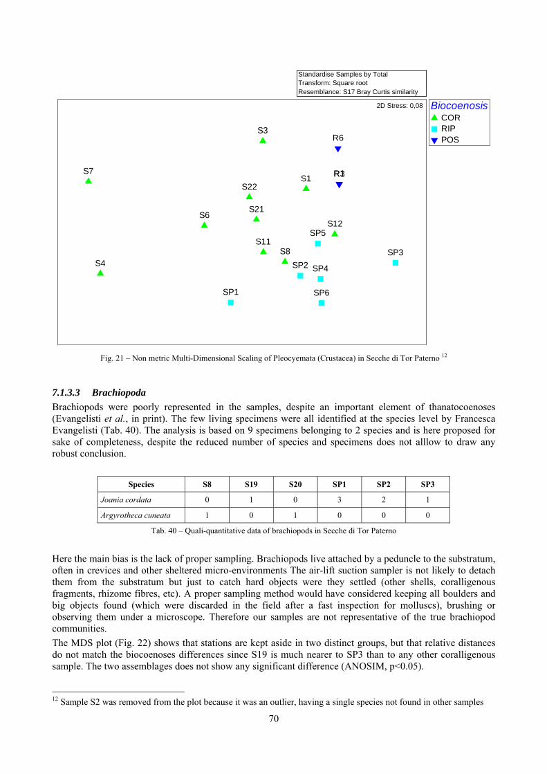
70

Fig. 21 – Non metric Multi-Dimensional Scaling of Pleocyemata (Crustacea) in Secche di Tor Paterno 12

7.1.3.3 Brachiopoda Brachiopods were poorly represented in the samples, despite an important element of thanatocoenoses (Evangelisti et al., in print). The few living specimens were all identified at the species level by Francesca Evangelisti (Tab. 40). The analysis is based on 9 specimens belonging to 2 species and is here proposed for sake of completeness, despite the reduced number of species and specimens does not alllow to draw any robust conclusion.

Species S8 S19 S20 SP1 SP2 SP3

Joania cordata 0 1 0 3 2 1

Argyrotheca cuneata 1 0 1 0 0 0

Tab. 40 – Quali-quantitative data of brachiopods in Secche di Tor Paterno

Here the main bias is the lack of proper sampling. Brachiopods live attached by a peduncle to the substratum, often in crevices and other sheltered micro-environments The air-lift suction sampler is not likely to detach them from the substratum but just to catch hard objects were they settled (other shells, coralligenous fragments, rhizome fibres, etc). A proper sampling method would have considered keeping all boulders and big objects found (which were discarded in the field after a fast inspection for molluscs), brushing or observing them under a microscope. Therefore our samples are not representative of the true brachiopod communities. The MDS plot (Fig. 22) shows that stations are kept aside in two distinct groups, but that relative distances do not match the biocoenoses differences since S19 is much nearer to SP3 than to any other coralligenous sample. The two assemblages does not show any significant difference (ANOSIM, p<0.05).

12 Sample S2 was removed from the plot because it was an outlier, having a single species not found in other samples

Standardise Samples by TotalTransform: Square rootResemblance: S17 Bray Curtis similarity

BiocoenosisCORRIPPOS

S1

S3

S4

S6

S7

S8S11

S12

S21

S22

SP1

SP2SP3

SP4

SP5

SP6

R1R3

R6

2D Stress: 0,08

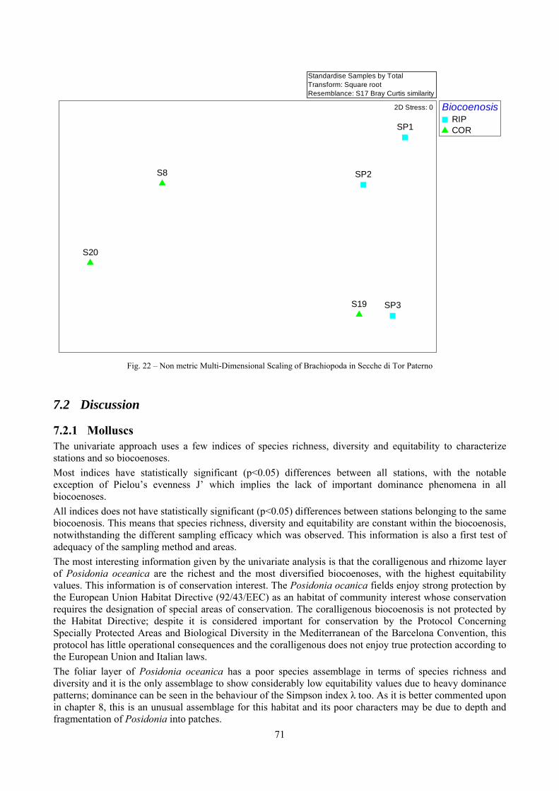
71

Fig. 22 – Non metric Multi-Dimensional Scaling of Brachiopoda in Secche di Tor Paterno

7.2 Discussion

7.2.1 Molluscs The univariate approach uses a few indices of species richness, diversity and equitability to characterize stations and so biocoenoses. Most indices have statistically significant (p<0.05) differences between all stations, with the notable exception of Pielou’s evenness J’ which implies the lack of important dominance phenomena in all biocoenoses. All indices does not have statistically significant (p<0.05) differences between stations belonging to the same biocoenosis. This means that species richness, diversity and equitability are constant within the biocoenosis, notwithstanding the different sampling efficacy which was observed. This information is also a first test of adequacy of the sampling method and areas. The most interesting information given by the univariate analysis is that the coralligenous and rhizome layer of Posidonia oceanica are the richest and the most diversified biocoenoses, with the highest equitability values. This information is of conservation interest. The Posidonia ocanica fields enjoy strong protection by the European Union Habitat Directive (92/43/EEC) as an habitat of community interest whose conservation requires the designation of special areas of conservation. The coralligenous biocoenosis is not protected by the Habitat Directive; despite it is considered important for conservation by the Protocol Concerning Specially Protected Areas and Biological Diversity in the Mediterranean of the Barcelona Convention, this protocol has little operational consequences and the coralligenous does not enjoy true protection according to the European Union and Italian laws. The foliar layer of Posidonia oceanica has a poor species assemblage in terms of species richness and diversity and it is the only assemblage to show considerably low equitability values due to heavy dominance patterns; dominance can be seen in the behaviour of the Simpson index λ too. As it is better commented upon in chapter 8, this is an unusual assemblage for this habitat and its poor characters may be due to depth and fragmentation of Posidonia into patches.

Standardise Samples by TotalTransform: Square rootResemblance: S17 Bray Curtis similarity

BiocoenosisRIPCORSP1

SP2

SP3

S8

S19

S20

2D Stress: 0

72

The detritic pools have a poor species assemblage too. This was predictable, and is confirmed by the values of the species richness indices and the diversity indices. However, the moderately high equitability indices show little dominance of any species. The comparison of indices between the different biocoenoses gave contrasting results depending on the index used and biocoenoses considered. Indices fail to evidence statistically significant differences between the biocoenoses in a consistent way and therefore if they are important descriptors of the species assemblages they are not useful for biocoenosis discrimination. The multivariate techniques manage to handle full quali-quantitative data matrices. Moreover, the techniques used do not need to reduce the number of variables (like PCA – Principal Component Analysis does). All the information is retained and the picture is more reliable. Clustering, Non metric Multi-Dimensional Scaling and similarity tests all confirm that four distinct species assemblages can be recognized with statistical significance (p<0.05): the detritic pools, the foliar and rhizome layers of Posidonia oceanica, the coralligenous. These assemblages usually have different typical species. The detritic is the most different biocoenosis whose typical species are not present elsewhere (Retusa mamillata and Pteromeris corbis). The foliar layer of Posidonia is well distinguishable too. Its most typical species (Chauvetia aff brunnea) is present also in the rhizomes. It has to be pointed out that nictemeral migrations from leaves to rhizomes and back have been documented in the Posidonia fields (Russo et al., 1984) and that our observations refer only to day-time assemblages. However, the day time species assemblage is the most typical of the leaves (Pérès & Picard, 1964). The rhizome layer of Posidonia is well distinguishable from its corresponding foliar level. It is a rich and diversified assemblage of species. Between its typical species there are filter feeders (e.g. Gouldia minima), proof of the importance of sedimentary enclaves between the rhizomes due to the action of the foliar layer which reduces water hydrodinamism. The coralligenous is rich and diversified too. Despite small sedimentary enclaves can be found here too, they are certainly most scattered and rare and the typical species are all microalgae herbivores (Bittium latreillii) or carnivorous (Nassarius incrassatus, Pollia scabra, Muricopsis cristata, Raphitoma linearis) gastropods. The rhizome layer and the coralligenous have close species assemblages and they have three typical species in common (Bittium latreillii, Muricopsis cristata and Raphitoma linearis). Pérès & Picard (1964) already highlighted that the foliar layer and the rhizome layer of Posidonia host two different biocoenoses and that the rhizome layer one is a sciaphilous community very similar to the coralligenous. Moreover, Bianchi et al (1989) suggest that the Posidonia meadows host four different and independent compartments (leaves, rhizomes, rhizomes infauna, vagile fauna). These approaches are confirmed by our data. With the main exception of the filter feeders Gouldia minima and Striarca lactea in the rhizomes, typical species are often carnivorous. The typifying role of carnivores in the biocoenoses is less easy to interpret. It may be due to high predation specialization, e.g. turrids are specialized for polychaetes. However, if carnivores are typifying species it may imply that their prey are not molluscs. Parasites never characterize any biocoenosis, notwithstanding their overall relative abundance (e.g. Triphoridae alone account for almost 100 specimens on 2700, 3.7%). This may be due to the fact that their host do not characterize biocoenoses. Triphoridae tend to be more frequent in the coralligenous, Cerithiopsidae in the rhizomes. Eulimidae and Pyramidellidae are not even present in the SIMPER results because their contribution is really marginal. This may be due to their rarity (especially for Eulimidae) and for their small size (Pyramidellidae, they may have been discarded in the sieving). The indices discussed at the beginning of this paragraph are able to describe characters of the assemblages and tell us to which extent assemblages from different biocoenoses have different characters. To answer the

73

question whether different biocoenoses host typical molluscan assemblages, the univariate approach is not useful. Multivariate approach has to be used since it values the information given by each single species in the assemblage. A striking example of this is that the foliar layer of Posidonia oceanica and the detritic biocoenoses are not different in terms of species richness, species diversity and equitability while these are clearly different on the basis of the analysis of the entire quali-quantitative data. This result shows clearly that indices are not suitable for discriminating between species assemblages, but they are only useful to further describe species assemblages or to compare samples from the same biocoenosis.

7.2.2 Other phyla Notwithstanding the several biases in the analyses described above, the result is somehow interesting and it is one of the very first carried out on such heterogeneous complex hard substrata. Concentrating our attention on the coralligenous vs Posidonia rhizomes differentiation, since they are the most similar environments with the most quantitatively significant samples, no other group shows neat and statistically significant differences like molluscs. As long as decapod crustaceans are concerned, this was already observed by García-Raso et al. (1996) despite in much shallower environments: they concluded that “these biotopes represent part of the habitat of the same decapod crustacean community” despite they host “differing quantitative species compositions” with “the high dominance of a small number of and different species”. Remarkable is the lack of differences in a very diverse group like polychaetes. It is important here to highlight that the result is potentiated by the bias induced by the splitting attitude in morphospecies segregation since this emphasizes differences in samples. The lack of significance of the differences of polychaetes and crustaceans may be due to their high vagility while molluscs are much less mobile animals. Brachiopods are too few in species and specimens to offer any conclusive remark, however, the lack of discriminating potential is probably due to the fact that both the coralligenous and the rhizomes offer the micro-environments needed by this group to settle and grow. These results are in accordance with what was already carried out on soft substrata (Gambi et al., 1982) where molluscs proved to be excellent descriptors.

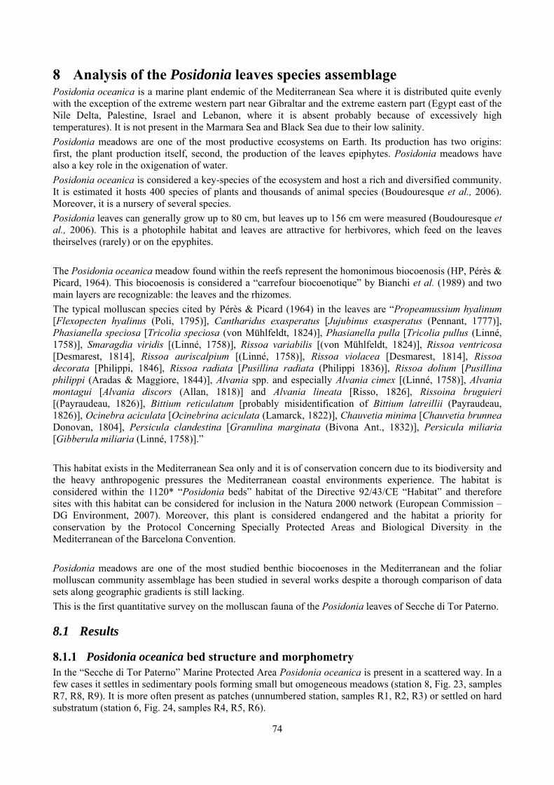
74

8 Analysis of the Posidonia leaves species assemblage Posidonia oceanica is a marine plant endemic of the Mediterranean Sea where it is distributed quite evenly with the exception of the extreme western part near Gibraltar and the extreme eastern part (Egypt east of the Nile Delta, Palestine, Israel and Lebanon, where it is absent probably because of excessively high temperatures). It is not present in the Marmara Sea and Black Sea due to their low salinity. Posidonia meadows are one of the most productive ecosystems on Earth. Its production has two origins: first, the plant production itself, second, the production of the leaves epiphytes. Posidonia meadows have also a key role in the oxigenation of water. Posidonia oceanica is considered a key-species of the ecosystem and host a rich and diversified community. It is estimated it hosts 400 species of plants and thousands of animal species (Boudouresque et al., 2006). Moreover, it is a nursery of several species. Posidonia leaves can generally grow up to 80 cm, but leaves up to 156 cm were measured (Boudouresque et al., 2006). This is a photophile habitat and leaves are attractive for herbivores, which feed on the leaves theirselves (rarely) or on the epyphites. The Posidonia oceanica meadow found within the reefs represent the homonimous biocoenosis (HP, Pérès & Picard, 1964). This biocoenosis is considered a “carrefour biocoenotique” by Bianchi et al. (1989) and two main layers are recognizable: the leaves and the rhizomes. The typical molluscan species cited by Pérès & Picard (1964) in the leaves are “Propeamussium hyalinum [Flexopecten hyalinus (Poli, 1795)], Cantharidus exasperatus [Jujubinus exasperatus (Pennant, 1777)], Phasianella speciosa [Tricolia speciosa (von Mühlfeldt, 1824)], Phasianella pulla [Tricolia pullus (Linné, 1758)], Smaragdia viridis [(Linné, 1758)], Rissoa variabilis [(von Mühlfeldt, 1824)], Rissoa ventricosa [Desmarest, 1814], Rissoa auriscalpium [(Linné, 1758)], Rissoa violacea [Desmarest, 1814], Rissoa decorata [Philippi, 1846], Rissoa radiata [Pusillina radiata (Philippi 1836)], Rissoa dolium [Pusillina philippi (Aradas & Maggiore, 1844)], Alvania spp. and especially Alvania cimex [(Linné, 1758)], Alvania montagui [Alvania discors (Allan, 1818)] and Alvania lineata [Risso, 1826], Rissoina bruguieri [(Payraudeau, 1826)], Bittium reticulatum [probably misidentification of Bittium latreillii (Payraudeau, 1826)], Ocinebra aciculata [Ocinebrina aciculata (Lamarck, 1822)], Chauvetia minima [Chauvetia brunnea Donovan, 1804], Persicula clandestina [Granulina marginata (Bivona Ant., 1832)], Persicula miliaria [Gibberula miliaria (Linné, 1758)].” This habitat exists in the Mediterranean Sea only and it is of conservation concern due to its biodiversity and the heavy anthropogenic pressures the Mediterranean coastal environments experience. The habitat is considered within the 1120* “Posidonia beds” habitat of the Directive 92/43/CE “Habitat” and therefore sites with this habitat can be considered for inclusion in the Natura 2000 network (European Commission – DG Environment, 2007). Moreover, this plant is considered endangered and the habitat a priority for conservation by the Protocol Concerning Specially Protected Areas and Biological Diversity in the Mediterranean of the Barcelona Convention. Posidonia meadows are one of the most studied benthic biocoenoses in the Mediterranean and the foliar molluscan community assemblage has been studied in several works despite a thorough comparison of data sets along geographic gradients is still lacking. This is the first quantitative survey on the molluscan fauna of the Posidonia leaves of Secche di Tor Paterno.

8.1 Results

8.1.1 Posidonia oceanica bed structure and morphometry In the “Secche di Tor Paterno” Marine Protected Area Posidonia oceanica is present in a scattered way. In a few cases it settles in sedimentary pools forming small but omogeneous meadows (station 8, Fig. 23, samples R7, R8, R9). It is more often present as patches (unnumbered station, samples R1, R2, R3) or settled on hard substratum (station 6, Fig. 24, samples R4, R5, R6).

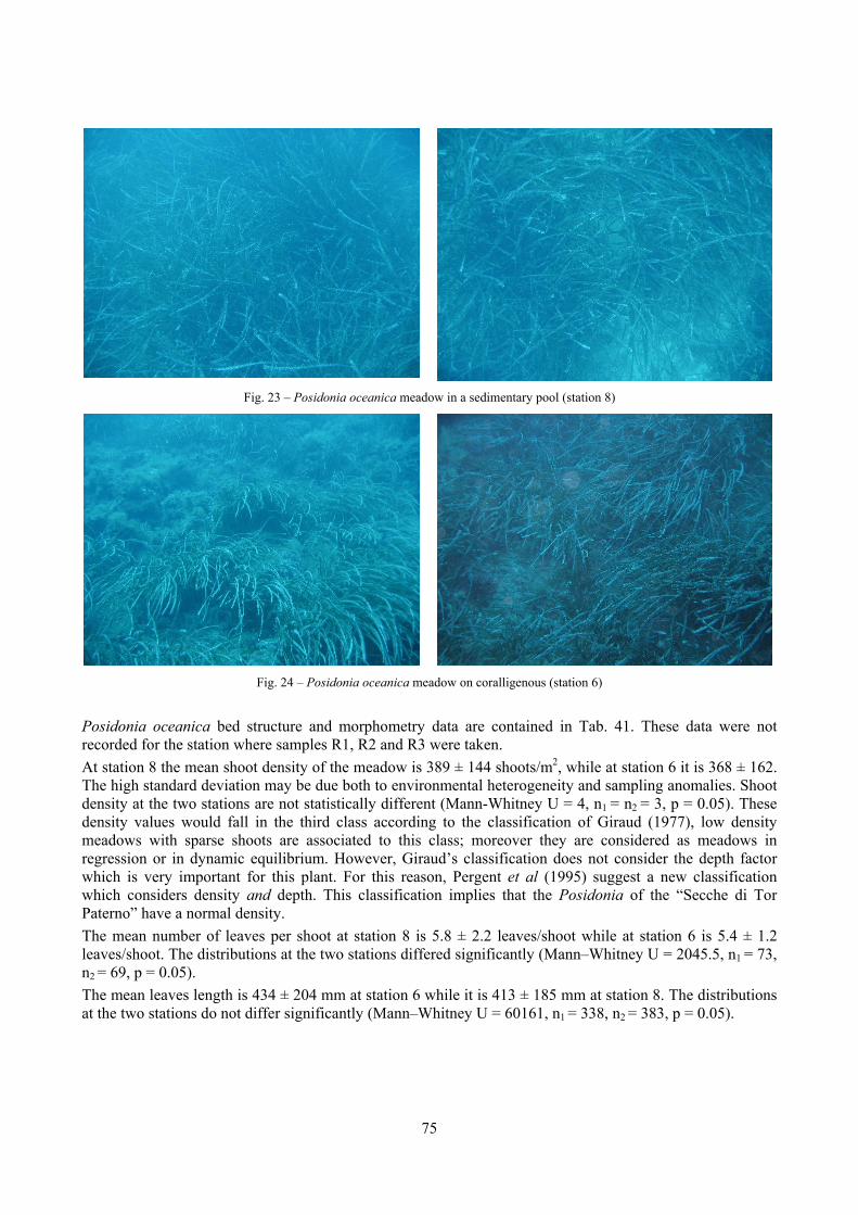
75

Fig. 23 – Posidonia oceanica meadow in a sedimentary pool (station 8)

Fig. 24 – Posidonia oceanica meadow on coralligenous (station 6)

Posidonia oceanica bed structure and morphometry data are contained in Tab. 41. These data were not recorded for the station where samples R1, R2 and R3 were taken. At station 8 the mean shoot density of the meadow is 389 ± 144 shoots/m2, while at station 6 it is 368 ± 162. The high standard deviation may be due both to environmental heterogeneity and sampling anomalies. Shoot density at the two stations are not statistically different (Mann-Whitney U = 4, n1 = n2 = 3, p = 0.05). These density values would fall in the third class according to the classification of Giraud (1977), low density meadows with sparse shoots are associated to this class; moreover they are considered as meadows in regression or in dynamic equilibrium. However, Giraud’s classification does not consider the depth factor which is very important for this plant. For this reason, Pergent et al (1995) suggest a new classification which considers density and depth. This classification implies that the Posidonia of the “Secche di Tor Paterno” have a normal density. The mean number of leaves per shoot at station 8 is 5.8 ± 2.2 leaves/shoot while at station 6 is 5.4 ± 1.2 leaves/shoot. The distributions at the two stations differed significantly (Mann–Whitney U = 2045.5, n1 = 73, n2 = 69, p = 0.05). The mean leaves length is 434 ± 204 mm at station 6 while it is 413 ± 185 mm at station 8. The distributions at the two stations do not differ significantly (Mann–Whitney U = 60161, n1 = 338, n2 = 383, p = 0.05).

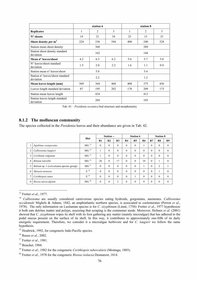
76

station 6 station 8

Replicates 1 2 3 1 2 3

N° shoots 14 21 34 25 15 33

Shoot density per m2 224 336 544 400 240 528

Station mean shoot density 368 389 Station shoot density standard deviation 162 144

Mean n° leaves/shoot 4.2 6.3 6.2 5.6 5.7 5.0 N° leaves/shoot standard deviation 1.5 2.0 2.2 1.6 1.1 0.9

Station mean n° leaves/shoot 5.8 5.4 Station n° leaves/shoot standard deviation 2.2 1.2

Mean leaves length [mm] 569 364 468 408 375 436

Leaves length standard deviation 87 195 202 178 209 175

Station mean leaves length 434 413 Station leaves length standard deviation 204 185

Tab. 41 – Posidonia oceanica bed structure and morphometry

8.1.2 The molluscan community The species collected in the Posidonia leaves and their abundance are given in Tab. 42.

Diet

Station -- Station 6 Station 8 R1 R2 R3 R4 R5 R6 R7 R8 R9

1 Jujubinus exasperatus MG 13 0 0 0 0 0 1 0 0 0

2 Calliostoma laugieri MG 14 1 0 0 0 0 0 0 0 0

3 Cerithium vulgatum MG 15 1 0 0 0 0 0 0 0 0

4 Bittium latreillii MG 16 20 0 17 0 0 10 0 1 0

5 Bittium sp. 1 (reticulatum species group) MG 17 0 0 0 0 0 1 0 2 1

6 Metaxia metaxae E 18 0 0 0 0 0 0 0 1 0

7 Cerithiopsis nana E 19 0 0 0 0 1 0 0 0 0

8 Rissoa auriscalpium MG 20 0 0 2 0 0 0 0 0 0

13 Fretter et al., 1977. 14 Calliostoma are usually considered carnivorous species eating hydroids, gorgonians, anemones. Calliostoma occidentale Mighels & Adams, 1842, an amphiatlantic northern species, is associated to coelenterates (Perron et al., 1978). The only information on Lusitanian species is for C. zizyphinum (Linné, 1758): Fretter et al., 1977 hypothesize it both eats detritus matter and polyps, assessing that scraping is the commoner mode. Moreover, Holmes et al. (2001) showed that C. zizyphinum wipes its shell with its foot gathering any matter (mainly microalgae) that has adhered to the pedal mucus present on the surface of its shell. In this way, it contributes to approximately one-fifth of its daily energetic requirement. Therefore, we consider it a microalgae herbivore and for C. laugieri we follow the same hypothesis. 15 Houbrick, 1992, for congeneric Indo-Pacific species. 16 Russo et al., 2002. 17 Fretter et al., 1981. 18 Bouchet, 1984. 19 Fretter et al., 1982 for the congeneric Cerithiopsis tubercularis (Montagu, 1803). 20 Fretter et al., 1978 for the congeneric Rissoa violacea Desmarest, 1814.

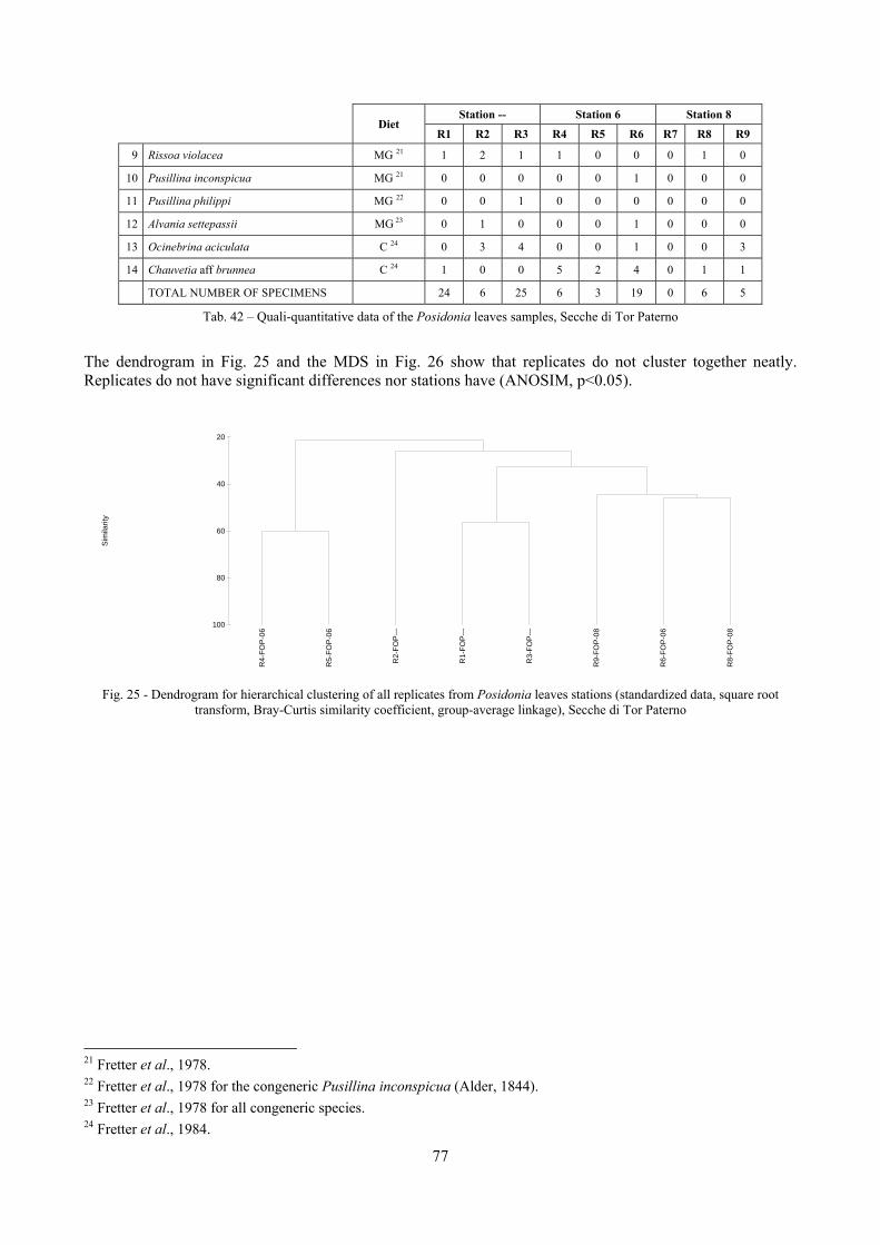
77

Diet

Station -- Station 6 Station 8 R1 R2 R3 R4 R5 R6 R7 R8 R9

9 Rissoa violacea MG 21 1 2 1 1 0 0 0 1 0

10 Pusillina inconspicua MG 21 0 0 0 0 0 1 0 0 0

11 Pusillina philippi MG 22 0 0 1 0 0 0 0 0 0

12 Alvania settepassii MG 23 0 1 0 0 0 1 0 0 0

13 Ocinebrina aciculata C 24 0 3 4 0 0 1 0 0 3

14 Chauvetia aff brunnea C 24 1 0 0 5 2 4 0 1 1

TOTAL NUMBER OF SPECIMENS 24 6 25 6 3 19 0 6 5

Tab. 42 – Quali-quantitative data of the Posidonia leaves samples, Secche di Tor Paterno

The dendrogram in Fig. 25 and the MDS in Fig. 26 show that replicates do not cluster together neatly. Replicates do not have significant differences nor stations have (ANOSIM, p<0.05).

Fig. 25 - Dendrogram for hierarchical clustering of all replicates from Posidonia leaves stations (standardized data, square root

transform, Bray-Curtis similarity coefficient, group-average linkage), Secche di Tor Paterno

21 Fretter et al., 1978. 22 Fretter et al., 1978 for the congeneric Pusillina inconspicua (Alder, 1844). 23 Fretter et al., 1978 for all congeneric species. 24 Fretter et al., 1984.

R4-

FOP

-06

R5-

FOP

-06

R2-

FOP

---

R1-

FOP

---

R3-

FOP

---

R9-

FOP

-08

R6-

FOP

-06

R8-

FOP

-08

100

80

60

40

20

Sim

ilarit

y

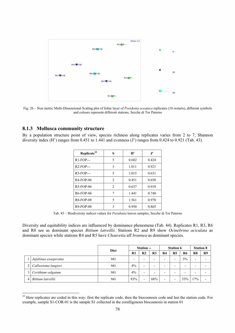
78

Fig. 26 – Non metric Multi-Dimensional Scaling plot of foliar layer of Posidonia oceanica replicates (10 restarts), different symbols

and colours represent different stations, Secche di Tor Paterno

8.1.3 Mollusca community structure By a population structure point of view, species richness along replicates varies from 2 to 7, Shannon diversity index (H’) ranges from 0.451 to 1.441 and evenness (J’) ranges from 0.424 to 0.921 (Tab. 43).

Replicate25 S H' J'

R1-FOP--- 5 0.682 0.424

R2-FOP--- 3 1.011 0.921

R3-FOP--- 5 1.015 0.631

R4-FOP-06 2 0.451 0.650

R5-FOP-06 2 0.637 0.918

R6-FOP-06 7 1.441 0.740

R8-FOP-08 5 1.561 0.970

R9-FOP-08 3 0.950 0.865

Tab. 43 – Biodiversity indices values for Posidonia leaves samples, Secche di Tor Paterno

Diversity and equitability indices are influenced by dominance phenomena (Tab. 44). Replicates R1, R3, R6 and R8 see as dominant species Bittium latreillii. Stations R2 and R9 show Ocinebrina aciculata as dominant species while stations R4 and R5 have Chauvetia aff brunnea as dominant species.

Diet

Station -- Station 6 Station 8 R1 R2 R3 R4 R5 R6 R8 R9

1 Jujubinus exasperatus MG - - - - - 5% - -

2 Calliostoma laugieri MG 4% - - - - - - -

3 Cerithium vulgatum MG 4% - - - - - - -

4 Bittium latreillii MG 83% - 68% - - 53% 17% -

25 Here replicates are coded in this way: first the replicate code, then the biocoenosis code and last the station code. For example, sample S1-COR-01 is the sample S1 collected in the coralligenous biocoenosis in station 01

S--

S6

S8R1-FOP---

R2-FOP---

R3-FOP---

R4-FOP-06

R5-FOP-06

R6-FOP-06

R8-FOP-08

R9-FOP-08

Stress: 0,1

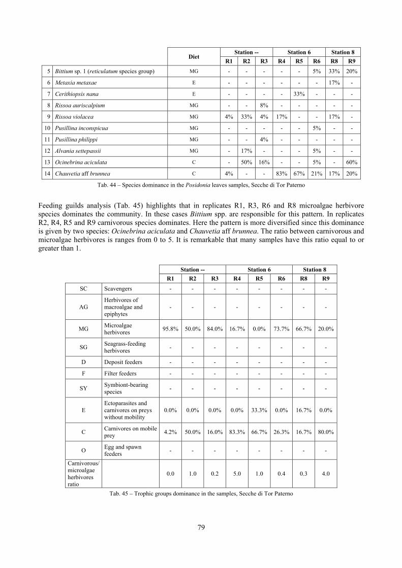
79

Diet

Station -- Station 6 Station 8 R1 R2 R3 R4 R5 R6 R8 R9

5 Bittium sp. 1 (reticulatum species group) MG - - - - - 5% 33% 20%

6 Metaxia metaxae E - - - - - - 17% -

7 Cerithiopsis nana E - - - - 33% - - -

8 Rissoa auriscalpium MG - - 8% - - - - -

9 Rissoa violacea MG 4% 33% 4% 17% - - 17% -

10 Pusillina inconspicua MG - - - - - 5% - -

11 Pusillina philippi MG - - 4% - - - - -

12 Alvania settepassii MG - 17% - - - 5% - -

13 Ocinebrina aciculata C - 50% 16% - - 5% - 60%

14 Chauvetia aff brunnea C 4% - - 83% 67% 21% 17% 20%

Tab. 44 – Species dominance in the Posidonia leaves samples, Secche di Tor Paterno

Feeding guilds analysis (Tab. 45) highlights that in replicates R1, R3, R6 and R8 microalgae herbivore species dominates the community. In these cases Bittium spp. are responsible for this pattern. In replicates R2, R4, R5 and R9 carnivorous species dominates. Here the pattern is more diversified since this dominance is given by two species: Ocinebrina aciculata and Chauvetia aff brunnea. The ratio between carnivorous and microalgae herbivores is ranges from 0 to 5. It is remarkable that many samples have this ratio equal to or greater than 1.

Station -- Station 6 Station 8 R1 R2 R3 R4 R5 R6 R8 R9

SC Scavengers - - - - - - - -

AG Herbivores of macroalgae and epiphytes

- - - - - - - -

MG Microalgae herbivores 95.8% 50.0% 84.0% 16.7% 0.0% 73.7% 66.7% 20.0%

SG Seagrass-feeding herbivores - - - - - - - -

D Deposit feeders - - - - - - - -

F Filter feeders - - - - - - - -

SY Symbiont-bearing species - - - - - - - -

E Ectoparasites and carnivores on preys without mobility

0.0% 0.0% 0.0% 0.0% 33.3% 0.0% 16.7% 0.0%

C Carnivores on mobile prey 4.2% 50.0% 16.0% 83.3% 66.7% 26.3% 16.7% 80.0%

O Egg and spawn feeders - - - - - - - -

Carnivorous/ microalgae herbivores ratio

0.0 1.0 0.2 5.0 1.0 0.4 0.3 4.0

Tab. 45 – Trophic groups dominance in the samples, Secche di Tor Paterno

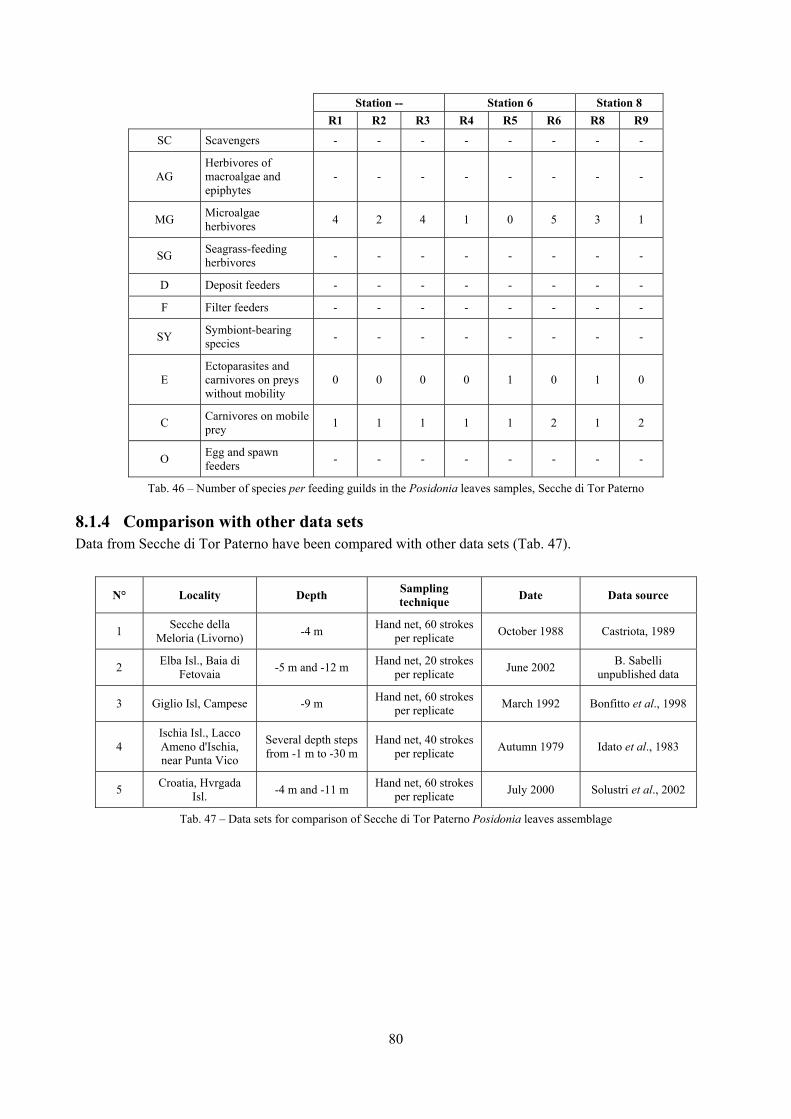
80

Station -- Station 6 Station 8 R1 R2 R3 R4 R5 R6 R8 R9

SC Scavengers - - - - - - - -

AG Herbivores of macroalgae and epiphytes

- - - - - - - -

MG Microalgae herbivores 4 2 4 1 0 5 3 1

SG Seagrass-feeding herbivores - - - - - - - -

D Deposit feeders - - - - - - - -

F Filter feeders - - - - - - - -

SY Symbiont-bearing species - - - - - - - -

E Ectoparasites and carnivores on preys without mobility

0 0 0 0 1 0 1 0

C Carnivores on mobile prey 1 1 1 1 1 2 1 2

O Egg and spawn feeders - - - - - - - -

Tab. 46 – Number of species per feeding guilds in the Posidonia leaves samples, Secche di Tor Paterno

8.1.4 Comparison with other data sets Data from Secche di Tor Paterno have been compared with other data sets (Tab. 47).

N° Locality Depth Sampling technique Date Data source

1 Secche della Meloria (Livorno) -4 m Hand net, 60 strokes

per replicate October 1988 Castriota, 1989

2 Elba Isl., Baia di Fetovaia -5 m and -12 m Hand net, 20 strokes

per replicate June 2002 B. Sabelli unpublished data

3 Giglio Isl, Campese -9 m Hand net, 60 strokes per replicate March 1992 Bonfitto et al., 1998

4 Ischia Isl., Lacco Ameno d'Ischia, near Punta Vico

Several depth steps from -1 m to -30 m

Hand net, 40 strokes per replicate Autumn 1979 Idato et al., 1983

5 Croatia, Hvrgada Isl. -4 m and -11 m Hand net, 60 strokes

per replicate July 2000 Solustri et al., 2002

Tab. 47 – Data sets for comparison of Secche di Tor Paterno Posidonia leaves assemblage

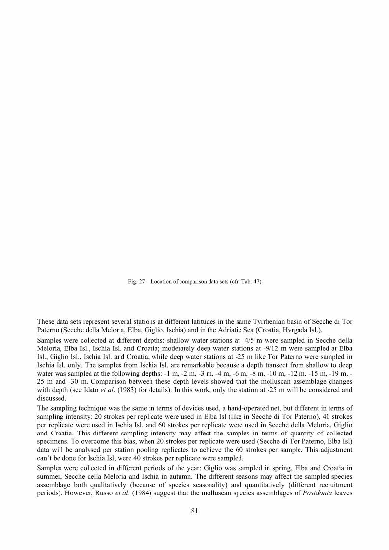
These data Paterno (SeSamples weMeloria, ElIsl., Giglio Ischia Isl. owater was s25 m and -with depth discussed. The samplinsampling inper replicatand Croatiaspecimens. data will becan’t be donSamples wesummer, Seassemblage periods). Ho

sets represencche della Mere collectedlba Isl., IschiIsl., Ischia I

only. The samsampled at th-30 m. Comp(see Idato et

ng techniquentensity: 20 se were used a. This diffeTo overcome analysed pne for Ischia ere collectedecche della M

both qualitowever, Rus

Fig. 2

nt several staMeloria, Elbad at differentia Isl. and Csl. and Croamples from Ihe following parison betwt al. (1983) f

e was the samstrokes per rein Ischia Isl

erent samplinme this bias, wper station po

Isl, were 40 d in differentMeloria and tatively (becsso et al. (19

27 – Location o

ations at diffea, Giglio, Ischt depths: sha

Croatia; modetia, while deIschia Isl. ardepths: -1 m

ween these dfor details). I

me in terms oeplicate werel. and 60 strong intensity when 20 stroooling replicstrokes per r

t periods of Ischia in au

cause of spe984) suggest

81

f comparison d

ferent latitudehia) and in thallow water serately deep eep water stare remarkabl

m, -2 m, -3 mdepth levels In this work,

of devices use used in Elbokes per rep

may affect okes per replicates to achireplicate werthe year: Gi

utumn. The decies seasonthat the mol

data sets (cfr. Ta

es in the samhe Adriatic Sstations at -4water statio

ations at -25 e because a

m, -4 m, -6 mshowed that only the sta

sed, a hand-oba Isl (like inlicate were uthe sample

icate were usieve the 60 sre sampled.glio was sam

different seasnality) and qlluscan spec

ab. 47)

me TyrrheniaSea (Croatia, 4/5 m were sons at -9/12 m

m like Tor Pdepth transe, -8 m, -10 mt the molluscation at -25 m

operated net, n Secche di used in Secces in terms osed (Secche strokes per s

mpled in sprsons may affquantitativelyies assembla

n basin of SeHvrgada Islsampled in Sm were samPaterno wereect from shalm, -12 m, -15can assemblm will be con

but differenTor Paterno

che della Meof quantity di Tor Patersample. This

ring, Elba anffect the samy (different ages of Posid

ecche di Tor.). Secche della

mpled at Elbae sampled inllow to deep5 m, -19 m, -age changesnsidered and

nt in terms of), 40 strokes

eloria, Giglioof collected

rno, Elba Isl)s adjustment

nd Croatia inmpled species

recruitmentdonia leaves

r

a a n p -s d

f s o d ) t

n s t s

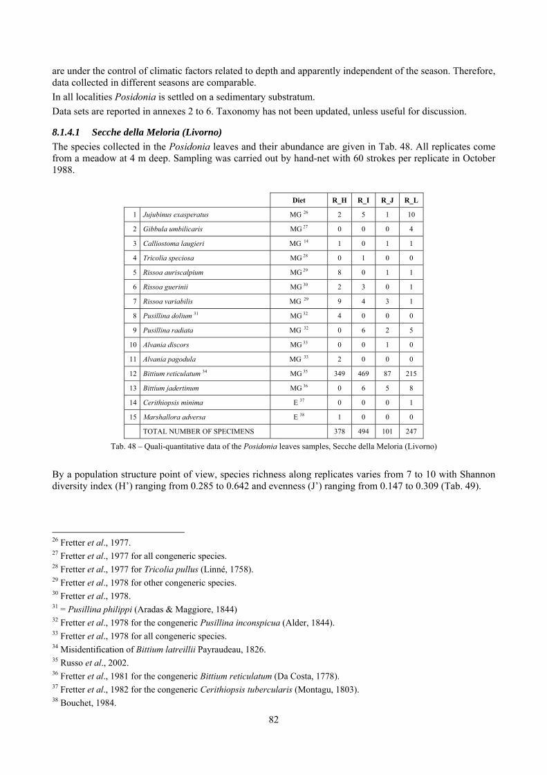
82

are under the control of climatic factors related to depth and apparently independent of the season. Therefore, data collected in different seasons are comparable. In all localities Posidonia is settled on a sedimentary substratum. Data sets are reported in annexes 2 to 6. Taxonomy has not been updated, unless useful for discussion.

8.1.4.1 Secche della Meloria (Livorno) The species collected in the Posidonia leaves and their abundance are given in Tab. 48. All replicates come from a meadow at 4 m deep. Sampling was carried out by hand-net with 60 strokes per replicate in October 1988.

Diet R_H R_I R_J R_L

1 Jujubinus exasperatus MG 26 2 5 1 10

2 Gibbula umbilicaris MG 27 0 0 0 4

3 Calliostoma laugieri MG 14 1 0 1 1

4 Tricolia speciosa MG 28 0 1 0 0

5 Rissoa auriscalpium MG 29 8 0 1 1

6 Rissoa guerinii MG 30 2 3 0 1

7 Rissoa variabilis MG 29 9 4 3 1

8 Pusillina dolium 31 MG 32 4 0 0 0

9 Pusillina radiata MG 32 0 6 2 5

10 Alvania discors MG 33 0 0 1 0

11 Alvania pagodula MG 33 2 0 0 0

12 Bittium reticulatum 34 MG 35 349 469 87 215

13 Bittium jadertinum MG 36 0 6 5 8

14 Cerithiopsis minima E 37 0 0 0 1

15 Marshallora adversa E 38 1 0 0 0

TOTAL NUMBER OF SPECIMENS 378 494 101 247

Tab. 48 – Quali-quantitative data of the Posidonia leaves samples, Secche della Meloria (Livorno)

By a population structure point of view, species richness along replicates varies from 7 to 10 with Shannon diversity index (H’) ranging from 0.285 to 0.642 and evenness (J’) ranging from 0.147 to 0.309 (Tab. 49).

26 Fretter et al., 1977. 27 Fretter et al., 1977 for all congeneric species. 28 Fretter et al., 1977 for Tricolia pullus (Linné, 1758). 29 Fretter et al., 1978 for other congeneric species. 30 Fretter et al., 1978. 31 = Pusillina philippi (Aradas & Maggiore, 1844) 32 Fretter et al., 1978 for the congeneric Pusillina inconspicua (Alder, 1844). 33 Fretter et al., 1978 for all congeneric species. 34 Misidentification of Bittium latreillii Payraudeau, 1826. 35 Russo et al., 2002. 36 Fretter et al., 1981 for the congeneric Bittium reticulatum (Da Costa, 1778). 37 Fretter et al., 1982 for the congeneric Cerithiopsis tubercularis (Montagu, 1803). 38 Bouchet, 1984.

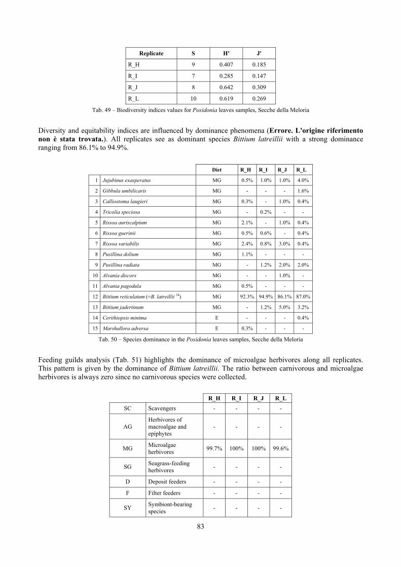
83

Replicate S H' J'

R_H 9 0.407 0.185

R_I 7 0.285 0.147

R_J 8 0.642 0.309

R_L 10 0.619 0.269

Tab. 49 – Biodiversity indices values for Posidonia leaves samples, Secche della Meloria

Diversity and equitability indices are influenced by dominance phenomena (Errore. L'origine riferimento non è stata trovata.). All replicates see as dominant species Bittium latreillii with a strong dominance ranging from 86.1% to 94.9%.

Diet R_H R_I R_J R_L

1 Jujubinus exasperatus MG 0.5% 1.0% 1.0% 4.0%

2 Gibbula umbilicaris MG - - - 1.6%

3 Calliostoma laugieri MG 0.3% - 1.0% 0.4%

4 Tricolia speciosa MG - 0.2% - -

5 Rissoa auriscalpium MG 2.1% - 1.0% 0.4%

6 Rissoa guerinii MG 0.5% 0.6% - 0.4%

7 Rissoa variabilis MG 2.4% 0.8% 3.0% 0.4%

8 Pusillina dolium MG 1.1% - - -

9 Pusillina radiata MG - 1.2% 2.0% 2.0%

10 Alvania discors MG - - 1.0% -

11 Alvania pagodula MG 0.5% - - -

12 Bittium reticulatum (=B. latreillii 34) MG 92.3% 94.9% 86.1% 87.0%

13 Bittium jadertinum MG - 1.2% 5.0% 3.2%

14 Cerithiopsis minima E - - - 0.4%

15 Marshallora adversa E 0.3% - - -

Tab. 50 – Species dominance in the Posidonia leaves samples, Secche della Meloria

Feeding guilds analysis (Tab. 51) highlights the dominance of microalgae herbivores along all replicates. This pattern is given by the dominance of Bittium latreillii. The ratio between carnivorous and microalgae herbivores is always zero since no carnivorous species were collected.

R_H R_I R_J R_L

SC Scavengers - - - -

AG Herbivores of macroalgae and epiphytes

- - - -

MG Microalgae herbivores 99.7% 100% 100% 99.6%

SG Seagrass-feeding herbivores - - - -

D Deposit feeders - - - -

F Filter feeders - - - -

SY Symbiont-bearing species - - - -

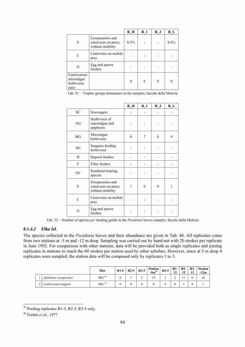
84

R_H R_I R_J R_L

E Ectoparasites and carnivores on preys without mobility

0.3% - - 0.4%

C Carnivores on mobile prey - - - -

O Egg and spawn feeders - - - -

Carnivorous/ microalgae herbivores ratio

0 0 0 0

Tab. 51 – Trophic groups dominance in the samples, Secche della Meloria

R_H R_I R_J R_L

SC Scavengers - - - -

AG Herbivores of macroalgae and epiphytes

- - - -

MG Microalgae herbivores 8 7 8 9

SG Seagrass-feeding herbivores - - - -

D Deposit feeders - - - -

F Filter feeders - - - -

SY Symbiont-bearing species - - - -

E Ectoparasites and carnivores on preys without mobility

1 0 0 1

C Carnivores on mobile prey - - - -

O Egg and spawn feeders - - - -

Tab. 52 – Number of species per feeding guilds in the Posidonia leaves samples, Secche della Meloria

8.1.4.2 Elba Isl. The species collected in the Posidonia leaves and their abundance are given in Tab. 48. All replicates come from two stations at -5 m and -12 m deep. Sampling was carried out by hand-net with 20 strokes per replicate in June 1992. For comparison with other stations, data will be provided both as single replicates and joining replicates in stations to reach the 60 strokes per station used by other scholars. However, since at 5 m deep 4 replicates were sampled, the station data will be composed only by replicates 1 to 3.

Diet R1-5 R2-5 R3-5 Station -5m39 R4-5 R1-

12 R2-12

R3-12

Station -12m

1 Jujubinus exasperatus MG 40 6 7 2 15 1 2 11 6 19

2 Calliostoma laugieri MG 14 0 0 0 0 0 0 1 0 1

39 Pooling replicates R1-5, R2-5, R3-5 only. 40 Fretter et al., 1977

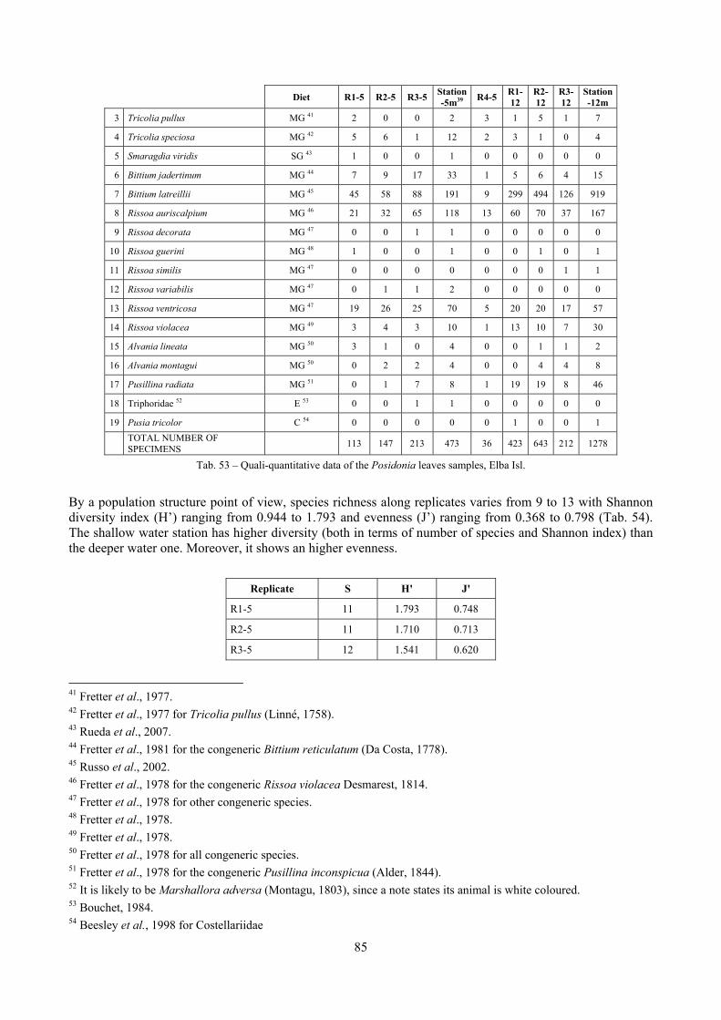
85

Diet R1-5 R2-5 R3-5 Station -5m39 R4-5 R1-

12 R2-12

R3-12

Station -12m

3 Tricolia pullus MG 41 2 0 0 2 3 1 5 1 7

4 Tricolia speciosa MG 42 5 6 1 12 2 3 1 0 4

5 Smaragdia viridis SG 43 1 0 0 1 0 0 0 0 0

6 Bittium jadertinum MG 44 7 9 17 33 1 5 6 4 15

7 Bittium latreillii MG 45 45 58 88 191 9 299 494 126 919

8 Rissoa auriscalpium MG 46 21 32 65 118 13 60 70 37 167

9 Rissoa decorata MG 47 0 0 1 1 0 0 0 0 0

10 Rissoa guerini MG 48 1 0 0 1 0 0 1 0 1

11 Rissoa similis MG 47 0 0 0 0 0 0 0 1 1

12 Rissoa variabilis MG 47 0 1 1 2 0 0 0 0 0

13 Rissoa ventricosa MG 47 19 26 25 70 5 20 20 17 57

14 Rissoa violacea MG 49 3 4 3 10 1 13 10 7 30

15 Alvania lineata MG 50 3 1 0 4 0 0 1 1 2

16 Alvania montagui MG 50 0 2 2 4 0 0 4 4 8

17 Pusillina radiata MG 51 0 1 7 8 1 19 19 8 46

18 Triphoridae 52 E 53 0 0 1 1 0 0 0 0 0

19 Pusia tricolor C 54 0 0 0 0 0 1 0 0 1

TOTAL NUMBER OF SPECIMENS 113 147 213 473 36 423 643 212 1278

Tab. 53 – Quali-quantitative data of the Posidonia leaves samples, Elba Isl.

By a population structure point of view, species richness along replicates varies from 9 to 13 with Shannon diversity index (H’) ranging from 0.944 to 1.793 and evenness (J’) ranging from 0.368 to 0.798 (Tab. 54). The shallow water station has higher diversity (both in terms of number of species and Shannon index) than the deeper water one. Moreover, it shows an higher evenness.

Replicate S H' J'

R1-5 11 1.793 0.748

R2-5 11 1.710 0.713

R3-5 12 1.541 0.620

41 Fretter et al., 1977. 42 Fretter et al., 1977 for Tricolia pullus (Linné, 1758). 43 Rueda et al., 2007. 44 Fretter et al., 1981 for the congeneric Bittium reticulatum (Da Costa, 1778). 45 Russo et al., 2002. 46 Fretter et al., 1978 for the congeneric Rissoa violacea Desmarest, 1814. 47 Fretter et al., 1978 for other congeneric species. 48 Fretter et al., 1978. 49 Fretter et al., 1978. 50 Fretter et al., 1978 for all congeneric species. 51 Fretter et al., 1978 for the congeneric Pusillina inconspicua (Alder, 1844). 52 It is likely to be Marshallora adversa (Montagu, 1803), since a note states its animal is white coloured. 53 Bouchet, 1984. 54 Beesley et al., 1998 for Costellariidae

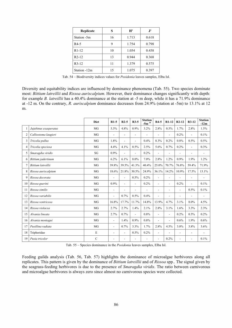
86

Replicate S H' J'

Station -5m 16 1.713 0.618

R4-5 9 1.754 0.798

R1-12 10 1.054 0.458

R2-12 13 0.944 0.368

R3-12 11 1.379 0.575

Station -12m 15 1.075 0.397

Tab. 54 – Biodiversity indices values for Posidonia leaves samples, Elba Isl.

Diversity and equitability indices are influenced by dominance phenomena (Tab. 55). Two species dominate most: Bittium latreillii and Rissoa auriscalpium. However, their dominance changes significantly with depth: for example B. latreillii has a 40.4% dominance at the station at -5 m deep, while it has a 71.9% dominance at -12 m. On the contrary, R. auriscalpium dominance decreases from 24.9% (station at -5m) to 13.1% at 12 m. Diet R1-5 R2-5 R3-5 Station

-5m 39 R4-5 R1-12 R2-12 R3-12 Station -12m

1 Jujubinus exasperatus MG 5.3% 4.8% 0.9% 3.2% 2.8% 0.5% 1.7% 2.8% 1.5%

2 Calliostoma laugieri MG - - - - - - 0.2% - 0.1%

3 Tricolia pullus MG 1.8% - - 0.4% 8.3% 0.2% 0.8% 0.5% 0.5%

4 Tricolia speciosa MG 4.4% 4.1% 0.5% 2.5% 5.6% 0.7% 0.2% - 0.3%

5 Smaragdia viridis SG 0.9% - - 0.2% - - - - -

6 Bittium jadertinum MG 6.2% 6.1% 8.0% 7.0% 2.8% 1.2% 0.9% 1.9% 1.2%

7 Bittium latreillii MG 39.8% 39.5% 41.3% 40.4% 25.0% 70.7% 76.8% 59.4% 71.9%

8 Rissoa auriscalpium MG 18.6% 21.8% 30.5% 24.9% 36.1% 14.2% 10.9% 17.5% 13.1%

9 Rissoa decorata MG - - 0.5% 0.2% - - - - -

10 Rissoa guerini MG 0.9% - - 0.2% - - 0.2% - 0.1%

11 Rissoa similis MG - - - - - - - 0.5% 0.1%

12 Rissoa variabilis MG - 0.7% 0.5% 0.4% - - - - -

13 Rissoa ventricosa MG 16.8% 17.7% 11.7% 14.8% 13.9% 4.7% 3.1% 8.0% 4.5%

14 Rissoa violacea MG 2.7% 2.7% 1.4% 2.1% 2.8% 3.1% 1.6% 3.3% 2.3%

15 Alvania lineata MG 2.7% 0.7% - 0.8% - - 0.2% 0.5% 0.2%

16 Alvania montagui MG - 1.4% 0.9% 0.8% - - 0.6% 1.9% 0.6%

17 Pusillina radiata MG - 0.7% 3.3% 1.7% 2.8% 4.5% 3.0% 3.8% 3.6%

18 Triphoridae E - - 0.5% 0.2% - - - - -

19 Pusia tricolor C - - - - - 0.2% - - 0.1%

Tab. 55 – Species dominance in the Posidonia leaves samples, Elba Isl.

Feeding guilds analysis (Tab. 56, Tab. 57) highlights the dominance of microalgae herbivores along all replicates. This pattern is given by the dominance of Bittium latreillii and of Rissoa spp.. The signal given by the seagrass-feeding herbivores is due to the presence of Smaragdia viridis. The ratio between carnivorous and microalgae herbivores is always zero since almost no carnivorous species were collected.

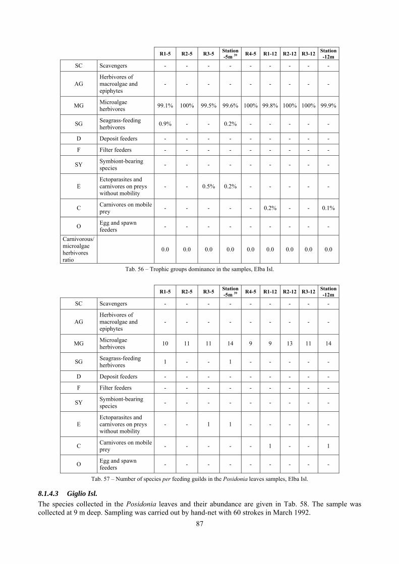
87

R1-5 R2-5 R3-5 Station -5m 39 R4-5 R1-12 R2-12 R3-12 Station

-12m

SC Scavengers - - - - - - - - -

AG Herbivores of macroalgae and epiphytes

- - - - - - - - -

MG Microalgae herbivores 99.1% 100% 99.5% 99.6% 100% 99.8% 100% 100% 99.9%

SG Seagrass-feeding herbivores 0.9% - - 0.2% - - - - -

D Deposit feeders - - - - - - - - -

F Filter feeders - - - - - - - - -

SY Symbiont-bearing species - - - - - - - - -

E Ectoparasites and carnivores on preys without mobility

- - 0.5% 0.2% - - - - -

C Carnivores on mobile prey - - - - - 0.2% - - 0.1%

O Egg and spawn feeders - - - - - - - - -

Carnivorous/ microalgae herbivores ratio

0.0 0.0 0.0 0.0 0.0 0.0 0.0 0.0 0.0

Tab. 56 – Trophic groups dominance in the samples, Elba Isl.

R1-5 R2-5 R3-5 Station -5m 39 R4-5 R1-12 R2-12 R3-12 Station

-12m

SC Scavengers - - - - - - - - -

AG Herbivores of macroalgae and epiphytes

- - - - - - - - -

MG Microalgae herbivores 10 11 11 14 9 9 13 11 14

SG Seagrass-feeding herbivores 1 - - 1 - - - - -

D Deposit feeders - - - - - - - - -

F Filter feeders - - - - - - - - -

SY Symbiont-bearing species - - - - - - - - -

E Ectoparasites and carnivores on preys without mobility

- - 1 1 - - - - -

C Carnivores on mobile prey - - - - - 1 - - 1

O Egg and spawn feeders - - - - - - - - -

Tab. 57 – Number of species per feeding guilds in the Posidonia leaves samples, Elba Isl.

8.1.4.3 Giglio Isl. The species collected in the Posidonia leaves and their abundance are given in Tab. 58. The sample was collected at 9 m deep. Sampling was carried out by hand-net with 60 strokes in March 1992.

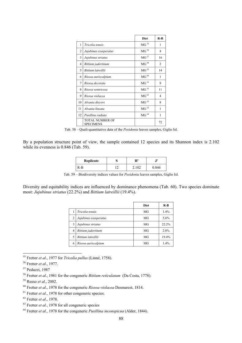
88

Diet R-B

1 Tricolia tenuis MG 55 1

2 Jujubinus exasperatus MG 56 4

3 Jujubinus striatus MG 57 16

4 Bittium jadertinum MG 58 2

5 Bittium latreillii MG 59 14

6 Rissoa auriscalpium MG 60 1

7 Rissoa decorata MG 61 9

8 Rissoa ventricosa MG 61 11

9 Rissoa violacea MG 62 4

10 Alvania discors MG 63 8

11 Alvania lineata MG 63 1

12 Pusillina radiata MG 64 1

TOTAL NUMBER OF SPECIMENS 72

Tab. 58 – Quali-quantitative data of the Posidonia leaves samples, Giglio Isl.

By a population structure point of view, the sample contained 12 species and its Shannon index is 2.102 while its evenness is 0.846 (Tab. 59).

Replicate S H' J'

R-B 12 2.102 0.846

Tab. 59 – Biodiversity indices values for Posidonia leaves samples, Giglio Isl.

Diversity and equitability indices are influenced by dominance phenomena (Tab. 60). Two species dominate most: Jujubinus striatus (22.2%) and Bittium latreillii (19.4%).

Diet R-B

1 Tricolia tenuis MG 1.4%

2 Jujubinus exasperatus MG 5.6%

3 Jujubinus striatus MG 22.2%

4 Bittium jadertinum MG 2.8%

5 Bittium latreillii MG 19.4%

6 Rissoa auriscalpium MG 1.4%

55 Fretter et al., 1977 for Tricolia pullus (Linné, 1758). 56 Fretter et al., 1977. 57 Peduzzi, 1987 58 Fretter et al., 1981 for the congeneric Bittium reticulatum (Da Costa, 1778). 59 Russo et al., 2002. 60 Fretter et al., 1978 for the congeneric Rissoa violacea Desmarest, 1814. 61 Fretter et al., 1978 for other congeneric species. 62 Fretter et al., 1978. 63 Fretter et al., 1978 for all congeneric species 64 Fretter et al., 1978 for the congeneric Pusillina inconspicua (Alder, 1844).

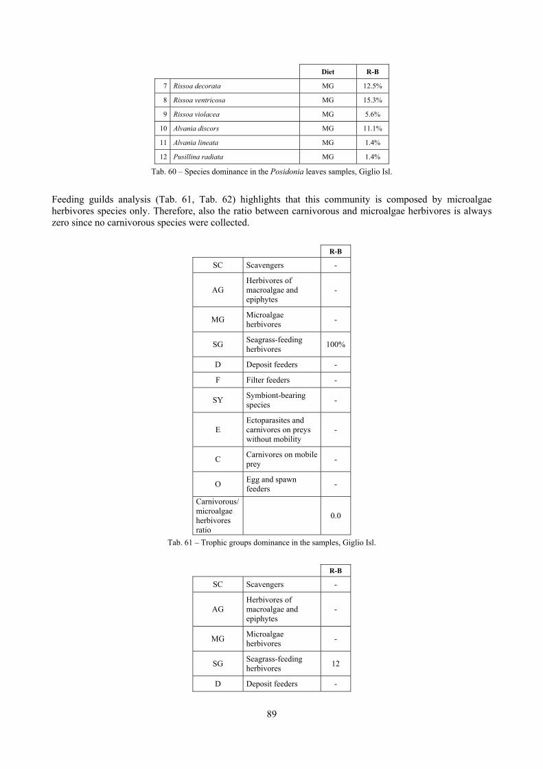
89

Diet R-B

7 Rissoa decorata MG 12.5%

8 Rissoa ventricosa MG 15.3%

9 Rissoa violacea MG 5.6%

10 Alvania discors MG 11.1%

11 Alvania lineata MG 1.4%

12 Pusillina radiata MG 1.4%

Tab. 60 – Species dominance in the Posidonia leaves samples, Giglio Isl.

Feeding guilds analysis (Tab. 61, Tab. 62) highlights that this community is composed by microalgae herbivores species only. Therefore, also the ratio between carnivorous and microalgae herbivores is always zero since no carnivorous species were collected.

R-B

SC Scavengers -

AG Herbivores of macroalgae and epiphytes

-

MG Microalgae herbivores -

SG Seagrass-feeding herbivores 100%

D Deposit feeders -

F Filter feeders -

SY Symbiont-bearing species -

E Ectoparasites and carnivores on preys without mobility

-

C Carnivores on mobile prey -

O Egg and spawn feeders -

Carnivorous/ microalgae herbivores ratio

0.0

Tab. 61 – Trophic groups dominance in the samples, Giglio Isl.

R-B

SC Scavengers -

AG Herbivores of macroalgae and epiphytes

-

MG Microalgae herbivores -

SG Seagrass-feeding herbivores 12

D Deposit feeders -

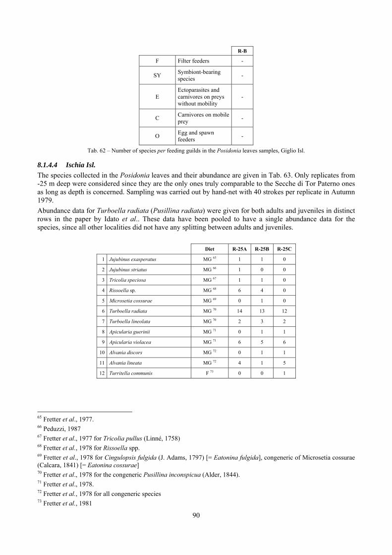
90

R-B

F Filter feeders -

SY Symbiont-bearing species -

E Ectoparasites and carnivores on preys without mobility

-

C Carnivores on mobile prey -

O Egg and spawn feeders -

Tab. 62 – Number of species per feeding guilds in the Posidonia leaves samples, Giglio Isl.

8.1.4.4 Ischia Isl. The species collected in the Posidonia leaves and their abundance are given in Tab. 63. Only replicates from -25 m deep were considered since they are the only ones truly comparable to the Secche di Tor Paterno ones as long as depth is concerned. Sampling was carried out by hand-net with 40 strokes per replicate in Autumn 1979. Abundance data for Turboella radiata (Pusillina radiata) were given for both adults and juveniles in distinct rows in the paper by Idato et al.. These data have been pooled to have a single abundance data for the species, since all other localities did not have any splitting between adults and juveniles.

Diet R-25A R-25B R-25C

1 Jujubinus exasperatus MG 65 1 1 0

2 Jujubinus striatus MG 66 1 0 0

3 Tricolia speciosa MG 67 1 1 0

4 Rissoella sp. MG 68 6 4 0

5 Microsetia cossurae MG 69 0 1 0

6 Turboella radiata MG 70 14 13 12

7 Turboella lineolata MG 70 2 3 2

8 Apicularia guerinii MG 71 0 1 1

9 Apicularia violacea MG 71 6 5 6

10 Alvania discors MG 72 0 1 1

11 Alvania lineata MG 72 4 1 5

12 Turritella communis F 73 0 0 1

65 Fretter et al., 1977. 66 Peduzzi, 1987 67 Fretter et al., 1977 for Tricolia pullus (Linné, 1758) 68 Fretter et al., 1978 for Rissoella spp. 69 Fretter et al., 1978 for Cingulopsis fulgida (J. Adams, 1797) [= Eatonina fulgida], congeneric of Microsetia cossurae (Calcara, 1841) [= Eatonina cossurae] 70 Fretter et al., 1978 for the congeneric Pusillina inconspicua (Alder, 1844). 71 Fretter et al., 1978. 72 Fretter et al., 1978 for all congeneric species 73 Fretter et al., 1981

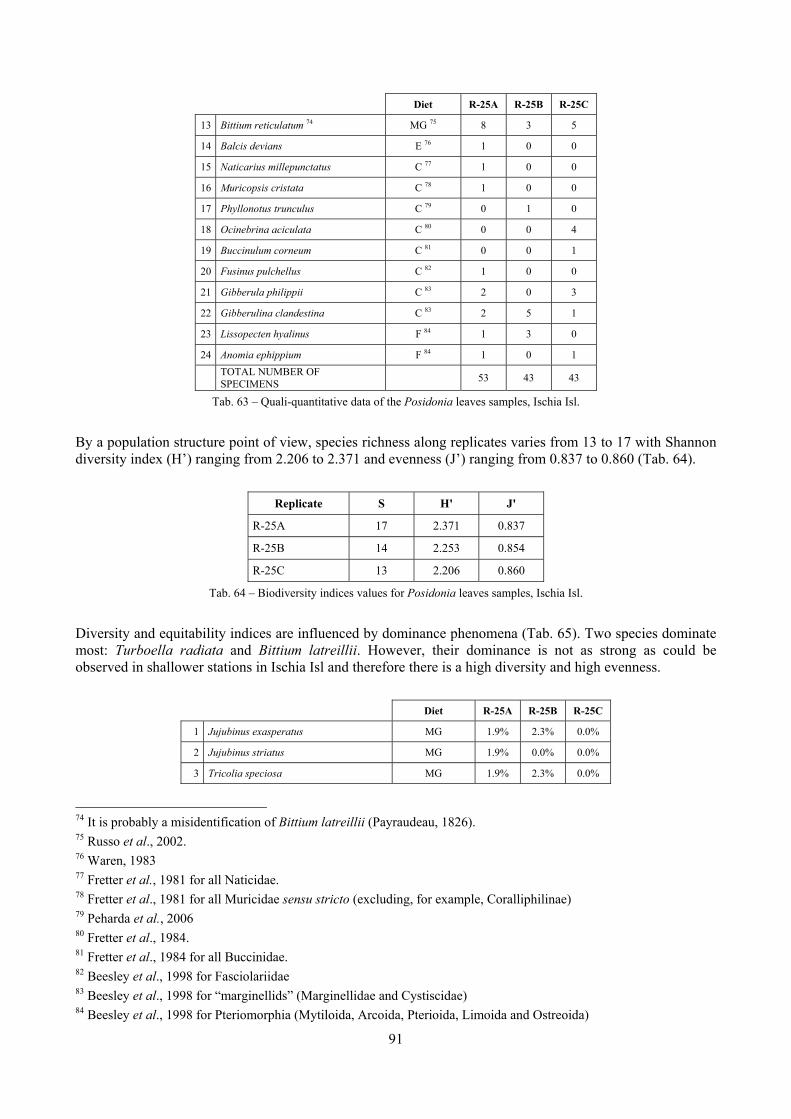
91

Diet R-25A R-25B R-25C

13 Bittium reticulatum 74 MG 75 8 3 5

14 Balcis devians E 76 1 0 0

15 Naticarius millepunctatus C 77 1 0 0

16 Muricopsis cristata C 78 1 0 0

17 Phyllonotus trunculus C 79 0 1 0

18 Ocinebrina aciculata C 80 0 0 4

19 Buccinulum corneum C 81 0 0 1

20 Fusinus pulchellus C 82 1 0 0

21 Gibberula philippii C 83 2 0 3

22 Gibberulina clandestina C 83 2 5 1

23 Lissopecten hyalinus F 84 1 3 0

24 Anomia ephippium F 84 1 0 1

TOTAL NUMBER OF SPECIMENS 53 43 43

Tab. 63 – Quali-quantitative data of the Posidonia leaves samples, Ischia Isl.

By a population structure point of view, species richness along replicates varies from 13 to 17 with Shannon diversity index (H’) ranging from 2.206 to 2.371 and evenness (J’) ranging from 0.837 to 0.860 (Tab. 64).

Replicate S H' J'

R-25A 17 2.371 0.837

R-25B 14 2.253 0.854

R-25C 13 2.206 0.860

Tab. 64 – Biodiversity indices values for Posidonia leaves samples, Ischia Isl.

Diversity and equitability indices are influenced by dominance phenomena (Tab. 65). Two species dominate most: Turboella radiata and Bittium latreillii. However, their dominance is not as strong as could be observed in shallower stations in Ischia Isl and therefore there is a high diversity and high evenness.

Diet R-25A R-25B R-25C

1 Jujubinus exasperatus MG 1.9% 2.3% 0.0%

2 Jujubinus striatus MG 1.9% 0.0% 0.0%

3 Tricolia speciosa MG 1.9% 2.3% 0.0%

74 It is probably a misidentification of Bittium latreillii (Payraudeau, 1826). 75 Russo et al., 2002. 76 Waren, 1983 77 Fretter et al., 1981 for all Naticidae. 78 Fretter et al., 1981 for all Muricidae sensu stricto (excluding, for example, Coralliphilinae) 79 Peharda et al., 2006 80 Fretter et al., 1984. 81 Fretter et al., 1984 for all Buccinidae. 82 Beesley et al., 1998 for Fasciolariidae 83 Beesley et al., 1998 for “marginellids” (Marginellidae and Cystiscidae) 84 Beesley et al., 1998 for Pteriomorphia (Mytiloida, Arcoida, Pterioida, Limoida and Ostreoida)

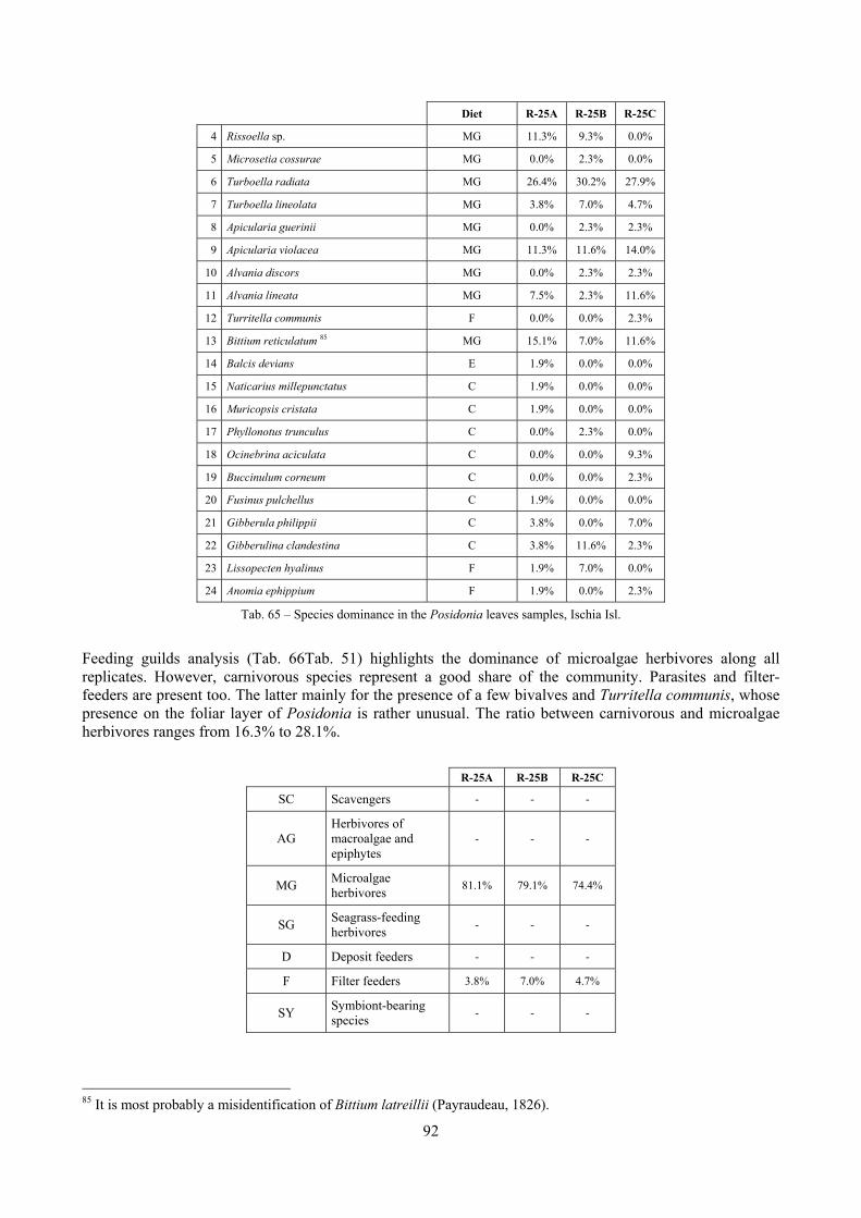
92

Diet R-25A R-25B R-25C

4 Rissoella sp. MG 11.3% 9.3% 0.0%

5 Microsetia cossurae MG 0.0% 2.3% 0.0%

6 Turboella radiata MG 26.4% 30.2% 27.9%

7 Turboella lineolata MG 3.8% 7.0% 4.7%

8 Apicularia guerinii MG 0.0% 2.3% 2.3%

9 Apicularia violacea MG 11.3% 11.6% 14.0%

10 Alvania discors MG 0.0% 2.3% 2.3%

11 Alvania lineata MG 7.5% 2.3% 11.6%

12 Turritella communis F 0.0% 0.0% 2.3%

13 Bittium reticulatum 85 MG 15.1% 7.0% 11.6%

14 Balcis devians E 1.9% 0.0% 0.0%

15 Naticarius millepunctatus C 1.9% 0.0% 0.0%

16 Muricopsis cristata C 1.9% 0.0% 0.0%

17 Phyllonotus trunculus C 0.0% 2.3% 0.0%

18 Ocinebrina aciculata C 0.0% 0.0% 9.3%

19 Buccinulum corneum C 0.0% 0.0% 2.3%

20 Fusinus pulchellus C 1.9% 0.0% 0.0%

21 Gibberula philippii C 3.8% 0.0% 7.0%

22 Gibberulina clandestina C 3.8% 11.6% 2.3%

23 Lissopecten hyalinus F 1.9% 7.0% 0.0%

24 Anomia ephippium F 1.9% 0.0% 2.3%

Tab. 65 – Species dominance in the Posidonia leaves samples, Ischia Isl.

Feeding guilds analysis (Tab. 66Tab. 51) highlights the dominance of microalgae herbivores along all replicates. However, carnivorous species represent a good share of the community. Parasites and filter-feeders are present too. The latter mainly for the presence of a few bivalves and Turritella communis, whose presence on the foliar layer of Posidonia is rather unusual. The ratio between carnivorous and microalgae herbivores ranges from 16.3% to 28.1%.

R-25A R-25B R-25C

SC Scavengers - - -

AG Herbivores of macroalgae and epiphytes

- - -

MG Microalgae herbivores 81.1% 79.1% 74.4%

SG Seagrass-feeding herbivores - - -

D Deposit feeders - - -

F Filter feeders 3.8% 7.0% 4.7%

SY Symbiont-bearing species - - -

85 It is most probably a misidentification of Bittium latreillii (Payraudeau, 1826).

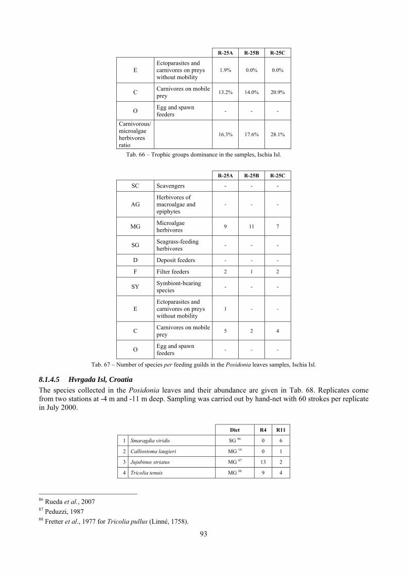
93

R-25A R-25B R-25C

E Ectoparasites and carnivores on preys without mobility

1.9% 0.0% 0.0%

C Carnivores on mobile prey 13.2% 14.0% 20.9%

O Egg and spawn feeders - - -

Carnivorous/ microalgae herbivores ratio

16.3% 17.6% 28.1%

Tab. 66 – Trophic groups dominance in the samples, Ischia Isl.

R-25A R-25B R-25C

SC Scavengers - - -

AG Herbivores of macroalgae and epiphytes

- - -

MG Microalgae herbivores 9 11 7

SG Seagrass-feeding herbivores - - -

D Deposit feeders - - -

F Filter feeders 2 1 2

SY Symbiont-bearing species - - -

E Ectoparasites and carnivores on preys without mobility

1 - -

C Carnivores on mobile prey 5 2 4

O Egg and spawn feeders - - -

Tab. 67 – Number of species per feeding guilds in the Posidonia leaves samples, Ischia Isl.

8.1.4.5 Hvrgada Isl, Croatia The species collected in the Posidonia leaves and their abundance are given in Tab. 68. Replicates come from two stations at -4 m and -11 m deep. Sampling was carried out by hand-net with 60 strokes per replicate in July 2000.

Diet R4 R11

1 Smaragdia viridis SG 86 0 6

2 Calliostoma laugieri MG 14 0 1

3 Jujubinus striatus MG 87 13 2

4 Tricolia tenuis MG 88 9 4

86 Rueda et al., 2007 87 Peduzzi, 1987 88 Fretter et al., 1977 for Tricolia pullus (Linné, 1758).

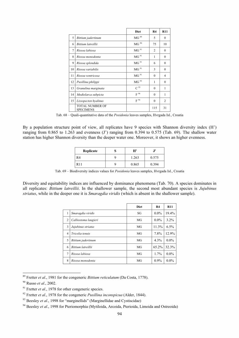
94

Diet R4 R11

5 Bittium jadertinum MG 89 5 0

6 Bittium latreillii MG 90 75 10

7 Rissoa labiosa MG 91 2 0

8 Rissoa monodonta MG 91 1 0

9 Rissoa splendida MG 91 6 0

10 Rissoa variabilis MG 91 3 0

11 Rissoa ventricosa MG 91 0 4

12 Pusillina philippi MG 92 1 0

13 Granulina marginata C 93 0 1

14 Modiolarca subpicta F 94 0 1

15 Lissopecten hyalinus F 94 0 2 TOTAL NUMBER OF SPECIMENS 115 31

Tab. 68 – Quali-quantitative data of the Posidonia leaves samples, Hvrgada Isl., Croatia

By a population structure point of view, all replicates have 9 species with Shannon diversity index (H’) ranging from 0.865 to 1.263 and evenness (J’) ranging from 0.394 to 0.575 (Tab. 69). The shallow water station has higher Shannon diversity than the deeper water one. Moreover, it shows an higher evenness.

Replicate S H' J'

R4 9 1.263 0.575

R11 9 0.865 0.394

Tab. 69 – Biodiversity indices values for Posidonia leaves samples, Hvrgada Isl., Croatia

Diversity and equitability indices are influenced by dominance phenomena (Tab. 70). A species dominates in all replicates: Bittium latreillii. In the shallower sample, the second most abundant species is Jujubinus striatus, while in the deeper one it is Smaragdia viridis (which is absent in the shallower sample).

Diet R4 R11

1 Smaragdia viridis SG 0.0% 19.4%

2 Calliostoma laugieri MG 0.0% 3.2%

3 Jujubinus striatus MG 11.3% 6.5%

4 Tricolia tenuis MG 7.8% 12.9%

5 Bittium jadertinum MG 4.3% 0.0%

6 Bittium latreillii MG 65.2% 32.3%

7 Rissoa labiosa MG 1.7% 0.0%

8 Rissoa monodonta MG 0.9% 0.0%

89 Fretter et al., 1981 for the congeneric Bittium reticulatum (Da Costa, 1778). 90 Russo et al., 2002. 91 Fretter et al., 1978 for other congeneric species. 92 Fretter et al., 1978 for the congeneric Pusillina inconspicua (Alder, 1844). 93 Beesley et al., 1998 for “marginellids” (Marginellidae and Cystiscidae) 94 Beesley et al., 1998 for Pteriomorphia (Mytiloida, Arcoida, Pterioida, Limoida and Ostreoida)

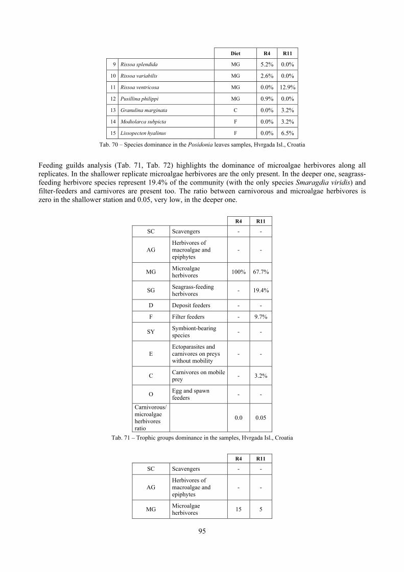
95

Diet R4 R11

9 Rissoa splendida MG 5.2% 0.0%

10 Rissoa variabilis MG 2.6% 0.0%

11 Rissoa ventricosa MG 0.0% 12.9%

12 Pusillina philippi MG 0.9% 0.0%

13 Granulina marginata C 0.0% 3.2%

14 Modiolarca subpicta F 0.0% 3.2%

15 Lissopecten hyalinus F 0.0% 6.5%

Tab. 70 – Species dominance in the Posidonia leaves samples, Hvrgada Isl., Croatia

Feeding guilds analysis (Tab. 71, Tab. 72) highlights the dominance of microalgae herbivores along all replicates. In the shallower replicate microalgae herbivores are the only present. In the deeper one, seagrass-feeding herbivore species represent 19.4% of the community (with the only species Smaragdia viridis) and filter-feeders and carnivores are present too. The ratio between carnivorous and microalgae herbivores is zero in the shallower station and 0.05, very low, in the deeper one.

R4 R11

SC Scavengers - -

AG Herbivores of macroalgae and epiphytes

- -

MG Microalgae herbivores 100% 67.7%

SG Seagrass-feeding herbivores - 19.4%

D Deposit feeders - -

F Filter feeders - 9.7%

SY Symbiont-bearing species - -

E Ectoparasites and carnivores on preys without mobility

- -

C Carnivores on mobile prey - 3.2%

O Egg and spawn feeders - -

Carnivorous/ microalgae herbivores ratio

0.0 0.05

Tab. 71 – Trophic groups dominance in the samples, Hvrgada Isl., Croatia

R4 R11

SC Scavengers - -

AG Herbivores of macroalgae and epiphytes

- -

MG Microalgae herbivores 15 5

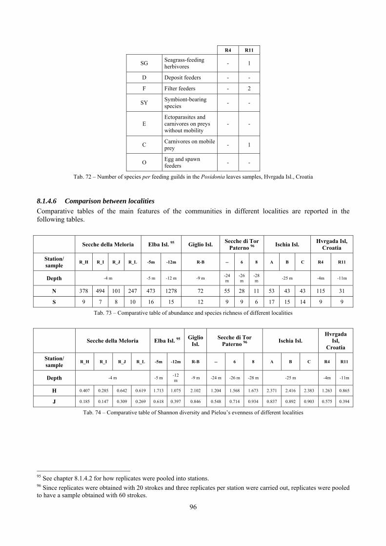
96

R4 R11

SG Seagrass-feeding herbivores - 1

D Deposit feeders - -

F Filter feeders - 2

SY Symbiont-bearing species - -

E Ectoparasites and carnivores on preys without mobility

- -

C Carnivores on mobile prey - 1

O Egg and spawn feeders - -

Tab. 72 – Number of species per feeding guilds in the Posidonia leaves samples, Hvrgada Isl., Croatia

8.1.4.6 Comparison between localities Comparative tables of the main features of the communities in different localities are reported in the following tables.

Secche della Meloria Elba Isl. 95 Giglio Isl. Secche di Tor Paterno 96 Ischia Isl. Hvrgada Isl,

Croatia

Station/ sample R_H R_I R_J R_L -5m -12m R-B -- 6 8 A B C R4 R11

Depth -4 m -5 m -12 m -9 m -24 m

-26 m

-28 m -25 m -4m -11m

N 378 494 101 247 473 1278 72 55 28 11 53 43 43 115 31

S 9 7 8 10 16 15 12 9 9 6 17 15 14 9 9

Tab. 73 – Comparative table of abundance and species richness of different localities

Secche della Meloria Elba Isl. 95 Giglio Isl.

Secche di Tor Paterno 96 Ischia Isl.

Hvrgada Isl,

Croatia

Station/ sample R_H R_I R_J R_L -5m -12m R-B -- 6 8 A B C R4 R11

Depth -4 m -5 m -12 m -9 m -24 m -26 m -28 m -25 m -4m -11m

H 0.407 0.285 0.642 0.619 1.713 1.075 2.102 1.204 1.568 1.673 2.371 2.416 2.383 1.263 0.865

J 0.185 0.147 0.309 0.269 0.618 0.397 0.846 0.548 0.714 0.934 0.837 0.892 0.903 0.575 0.394

Tab. 74 – Comparative table of Shannon diversity and Pielou’s evenness of different localities

95 See chapter 8.1.4.2 for how replicates were pooled into stations. 96 Since replicates were obtained with 20 strokes and three replicates per station were carried out, replicates were pooled to have a sample obtained with 60 strokes.

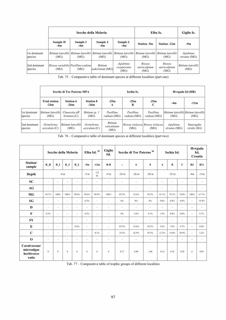
97

Secche della Meloria Elba Is. Giglio Is.

Sample H

-4m Sample I

-4m Sample J

-4m Sample L

-4m Station -5m Station -12m -9m

1st dominant species

Bittium latreillii (MG)

Bittium latreillii (MG)

Bittium latreillii (MG)

Bittium latreillii (MG)

Bittium latreillii (MG)

Bittium latreillii (MG)

Jujubinus striatus (MG)

2nd dominant species

Rissoa variabilis (MG)

Pusillina radiata (MG)

Bittium jadertinum (MG)

Jujubinus exasperatus

(MG)

Rissoa auriscalpium

(MG)

Rissoa auriscalpium

(MG)

Bittium latreillii (MG)

Tab. 75 – Comparative table of dominant species at different localities (part one)

Secche di Tor Paterno MPA Ischia Is. Hvrgada Isl (HR)

Trial station -24m

Station 6 -26m

Station 8 -26m

-25m A

-25m B

-25m C -4m -11m

1st dominant species

Bittium latreillii (MG)

Chauvetia aff brunnea (C)

Bittium sp. 1 (MG)

Pusillina radiata (MG)

Pusillina radiata (MG)

Pusillina radiata (MG)

Bittium latreillii (MG)

Bittium latreillii (MG)

2nd dominant species

Ocinebrina aciculata (C)

Bittium latreillii (MG)

Ocinebrina aciculata (C)

Bittium reticulatum

(MG)

Rissoa violacea (MG)

Rissoa violacea (MG)

Jujubinus striatus (MG)

Smaragdia viridis (SG)

Tab. 76 – Comparative table of dominant species at different localities (part two)

Secche della Meloria Elba Isl. 95 Giglio Isl. Secche di Tor Paterno 96 Ischia Isl.

Hvrgada Isl,

Croatia

Station/ sample R_H R_I R_J R_L -5m -12m R-B -- 6 8 A B C R4 R11

Depth -4 m -5 m -12 m -9 m -24 m -26 m -28 m -25 m -4m -11m

SC - - - - - - - - - - - - - - -

AG - - - - - - - - - - - - - - -

MG 99.7% 100% 100% 99.6% 99.6% 99.9% 100% 85.5% 53.6% 45.5% 81.1% 79.1% 74.4% 100% 67.7%

SG - - - - 0.2% - - 0% 0% 0% 0.0% 0.0% 0.0% - 19.4%

D - - - - - - - - - - - - - - -

F 0.3% - - - 0.2% - - 0% 3.6% 9.1% 1.9% 0.0% 0.0% - 9.7%

SY - - - - - - - - - - - - - - -

E - - - 0.4% - - - 85.5% 53.6% 45.5% 3.8% 7.0% 4.7% - 0.0%

C - - - - - 0.1% - 14.5% 42.9% 45.5% 13.2% 14.0% 20.9% - 3.2%

O - - - - - - - - - - - - - - -

Carnivorous/ microalgae herbivores

ratio

0 0 0 0 0 0 0 0.17 0.80 1.00 0.16 0.18 0.28 0 0.05

Tab. 77 – Comparative table of trophic groups of different localities

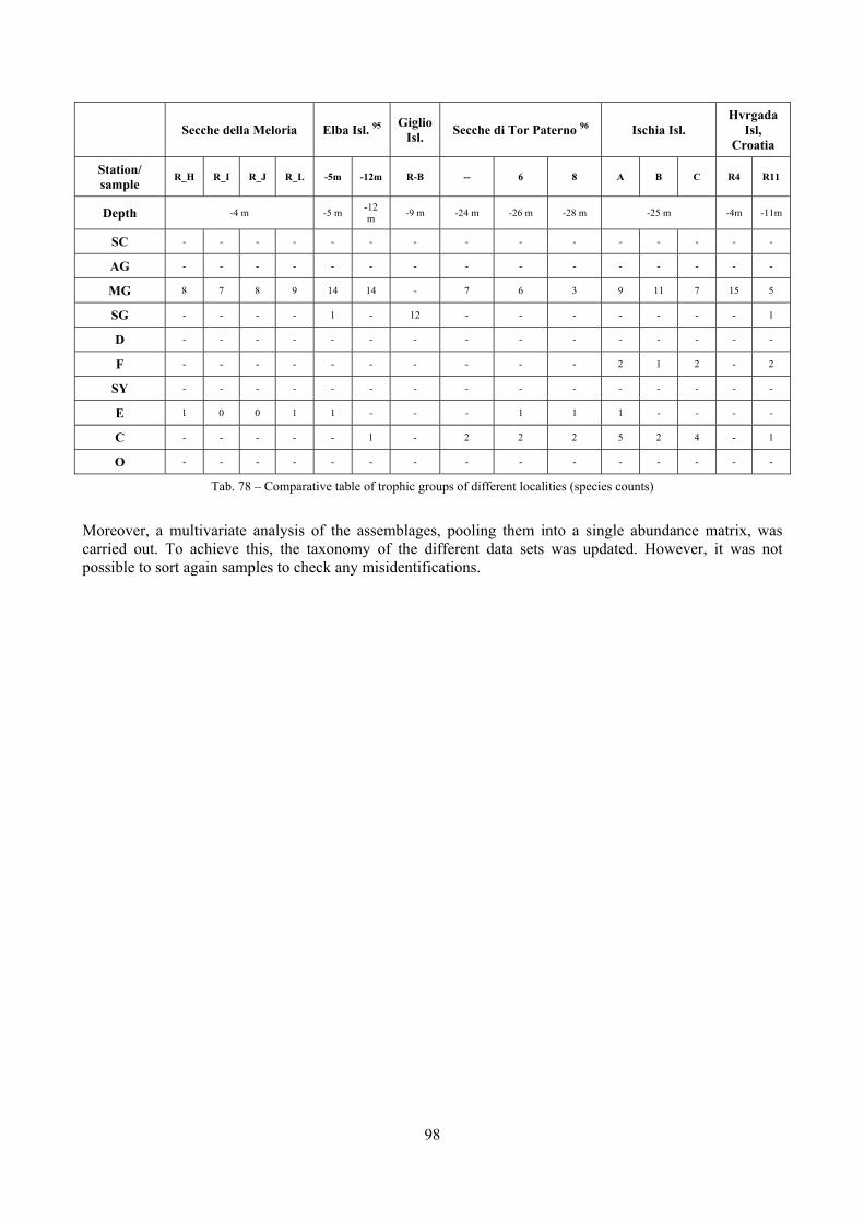
98

Secche della Meloria Elba Isl. 95 Giglio Isl. Secche di Tor Paterno 96 Ischia Isl.

Hvrgada Isl,

Croatia

Station/ sample R_H R_I R_J R_L -5m -12m R-B -- 6 8 A B C R4 R11

Depth -4 m -5 m -12 m -9 m -24 m -26 m -28 m -25 m -4m -11m

SC - - - - - - - - - - - - - - -

AG - - - - - - - - - - - - - - -

MG 8 7 8 9 14 14 - 7 6 3 9 11 7 15 5

SG - - - - 1 - 12 - - - - - - - 1

D - - - - - - - - - - - - - - -

F - - - - - - - - - - 2 1 2 - 2

SY - - - - - - - - - - - - - - -

E 1 0 0 1 1 - - - 1 1 1 - - - -

C - - - - - 1 - 2 2 2 5 2 4 - 1

O - - - - - - - - - - - - - - -

Tab. 78 – Comparative table of trophic groups of different localities (species counts)

Moreover, a multivariate analysis of the assemblages, pooling them into a single abundance matrix, was carried out. To achieve this, the taxonomy of the different data sets was updated. However, it was not possible to sort again samples to check any misidentifications.

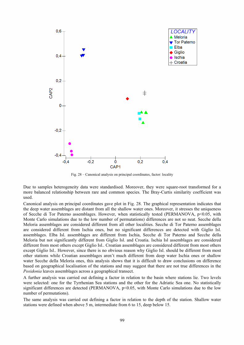
Due to sammore balanused. Canonical athe deep waof Secche dMonte CarlMeloria assare consideassemblageMeloria butdifferent froexcept Giglother statiowater Secchbased on gePosidonia lA further awere selectsignificant dnumber of pThe same astations wer

mples heterogced relations

analysis on pater assembladi Tor Paterlo simulationsemblages arered differens. Elba Isl. t not significom most othelio Isl.. Howns while Crhe della Meleographical leaves assembnalysis was ed: one for differences apermutationsanalysis wasre defined wh

Fig. 28 – Ca

geneity data ship between

principal cooages are distrno assemblans due to there considerednt from Isch

assemblagecantly differers except G

wever, since troatian assemloria ones, thlocalisation oblages acroscarried out the Tyrrheniare detected s). carried out hen above 5

anonical analys

were standan rare and c

ordinates gavtant from all ages. Howeve low numbed different fhia ones, bus are differe

rent from Giiglio Isl.. Crothere is no obmblages arenhis analysis of the stations a geographdefining a fian Sea stati(PERMANO

defining a fm, intermed

99

sis on principal

ardised. Morcommon spe

ve plot in Figthe shallow

ver, when ster of permutfrom all otheut no signifent from Isciglio Isl. andoatian assembvious reason’t much difshows that

ns and may hical transectfactor in relaions and theOVA, p<0.0

factor in reldiate from 6 t

coordinates, fa

reover, they cies. The Br

g. 28. The grwater ones.

tatistically tetations) diffeer localities. ficant differechia, Secched Croatia. Is

mblages are con why Giglifferent from it is difficulsuggest that t. ation to the be other for th5, with Mon

ation to the to 15, deep b

ctor: locality

were squareray-Curtis si

raphical reprMoreover, i

ested (PERMerences are n

Secche di Tences are dee di Tor Pachia Isl asse

considered diio Isl. shoulddeep water

lt to draw cothere are no

basin where he Adriatic Snte Carlo sim

depth of thebelow 15.

e-root transfimilarity coe

resentation int stresses the

MANOVA, pnot so neat. STor Paterno etected withaterno and Semblages areifferent fromd be differenr Ischia onesonclusions oot true differ

stations lie.Sea one. Nomulations du

e station. Sh

formed for aefficient was

ndicates thate uniquenessp<0.05, withSecche dellaassemblages

h Giglio Isl.Secche dellae considered

m most othersnt from mosts or shallow

on differencerences in the

. Two levelso statisticallyue to the low

hallow water

a s

t s h a s . a d s t

w e e

s y w

r

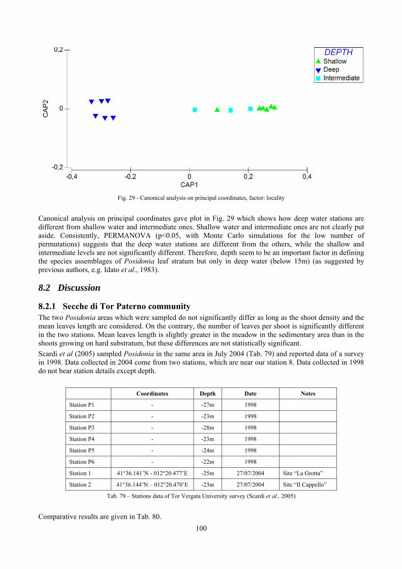
Canonical adifferent froaside. Conpermutationintermediatethe species previous au

8.2 Disc

8.2.1 SecThe two Pomean leavesin the two sshoots growScardi et alin 1998. Dado not bear

S

S

S

S

S

S

S

S

Comparativ

analysis on pom shallow wsistently, PE

ns) suggests e levels are nassemblage

uthors, e.g. Id

cussion

cche di Toosidonia areas length are stations. Meawing on hard l (2005) sampata collected station detai

tation P1

tation P2

tation P3

tation P4

tation P5

tation P6

tation 1

tation 2

T

ve results are

Fig. 29 - Ca

principal coowater and intERMANOVthat the dee

not significans of Posidon

dato et al., 19

or Paternoas which werconsidered. an leaves lensubstratum, pled Posidonin 2004 com

ils except dep

Coo

41°36.141’N

41°36.144’N

Tab. 79 – Statio

given in Tab

anonical analys

ordinates gavtermediate o

VA (p<0.05, ep water stantly differentnia leaf stra983).

o communire sampled dOn the contr

ngth is slightbut these dif

nia in the samme from two pth.

ordinates

-

-

-

-

-

-

N - 012°20.477

N – 012°20.470

ons data of Tor V

b. 80. 100

is on principal

ve plot in Fiones. Shallow

with Montations are dit. Therefore,

atum but onl

ity do not signifirary, the numtly greater infferences areme area in Justations, wh

Depth

-27m

-23m

-28m

-23m

-24m

-22m

7’E -25m

0’E -23m

Vergata Univer

coordinates, fac

ig. 29 whichw water and te Carlo simifferent from, depth seem ly in deep w

icantly differmber of leaven the meadowe not statisticuly 2004 (Taich are near

Date

1998

1998

1998

1998

1998

1998

27/07/2

27/07/2

rsity survey (Sc

ctor: locality

h shows howintermediatemulations fo

m the others,to be an imp

water (below

r as long as tes per shoot w in the sedically significaab. 79) and rour station 8

e

8

8

8

8

8

8

2004 Site

2004 Site

cardi et al., 200

w deep watere ones are nofor the low , while the portant facto

w 15m) (as s

the shoot denis significanmentary areaant. reported data8. Data colle

Notes

e “La Grotta”

e “Il Cappello”

5)

r stations areot clearly put

number ofshallow andr in defininguggested by

nsity and thently differenta than in the

a of a surveycted in 1998

e t f d g y

e t e

y 8

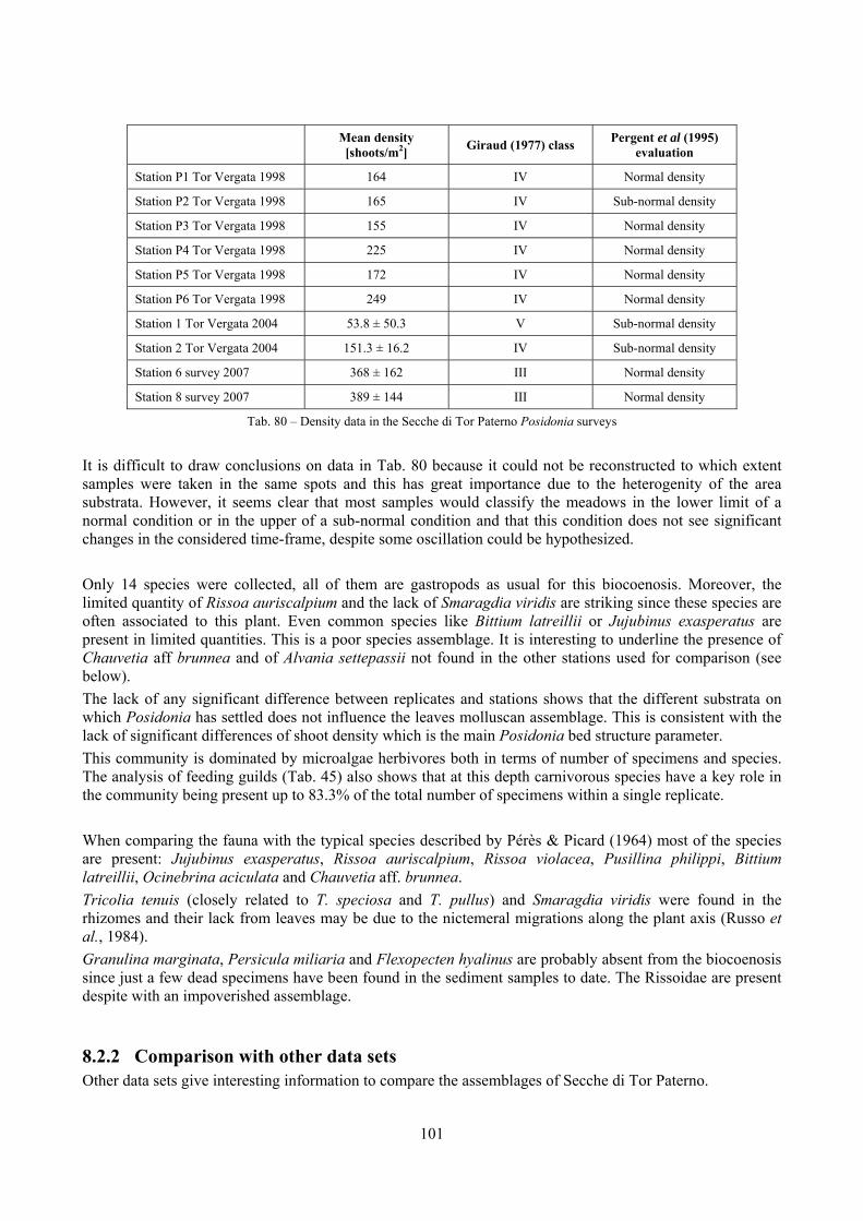
101

Mean density [shoots/m2] Giraud (1977) class Pergent et al (1995)

evaluation

Station P1 Tor Vergata 1998 164 IV Normal density

Station P2 Tor Vergata 1998 165 IV Sub-normal density

Station P3 Tor Vergata 1998 155 IV Normal density

Station P4 Tor Vergata 1998 225 IV Normal density

Station P5 Tor Vergata 1998 172 IV Normal density

Station P6 Tor Vergata 1998 249 IV Normal density

Station 1 Tor Vergata 2004 53.8 ± 50.3 V Sub-normal density

Station 2 Tor Vergata 2004 151.3 ± 16.2 IV Sub-normal density

Station 6 survey 2007 368 ± 162 III Normal density

Station 8 survey 2007 389 ± 144 III Normal density

Tab. 80 – Density data in the Secche di Tor Paterno Posidonia surveys

It is difficult to draw conclusions on data in Tab. 80 because it could not be reconstructed to which extent samples were taken in the same spots and this has great importance due to the heterogenity of the area substrata. However, it seems clear that most samples would classify the meadows in the lower limit of a normal condition or in the upper of a sub-normal condition and that this condition does not see significant changes in the considered time-frame, despite some oscillation could be hypothesized. Only 14 species were collected, all of them are gastropods as usual for this biocoenosis. Moreover, the limited quantity of Rissoa auriscalpium and the lack of Smaragdia viridis are striking since these species are often associated to this plant. Even common species like Bittium latreillii or Jujubinus exasperatus are present in limited quantities. This is a poor species assemblage. It is interesting to underline the presence of Chauvetia aff brunnea and of Alvania settepassii not found in the other stations used for comparison (see below). The lack of any significant difference between replicates and stations shows that the different substrata on which Posidonia has settled does not influence the leaves molluscan assemblage. This is consistent with the lack of significant differences of shoot density which is the main Posidonia bed structure parameter. This community is dominated by microalgae herbivores both in terms of number of specimens and species. The analysis of feeding guilds (Tab. 45) also shows that at this depth carnivorous species have a key role in the community being present up to 83.3% of the total number of specimens within a single replicate. When comparing the fauna with the typical species described by Pérès & Picard (1964) most of the species are present: Jujubinus exasperatus, Rissoa auriscalpium, Rissoa violacea, Pusillina philippi, Bittium latreillii, Ocinebrina aciculata and Chauvetia aff. brunnea. Tricolia tenuis (closely related to T. speciosa and T. pullus) and Smaragdia viridis were found in the rhizomes and their lack from leaves may be due to the nictemeral migrations along the plant axis (Russo et al., 1984). Granulina marginata, Persicula miliaria and Flexopecten hyalinus are probably absent from the biocoenosis since just a few dead specimens have been found in the sediment samples to date. The Rissoidae are present despite with an impoverished assemblage.

8.2.2 Comparison with other data sets Other data sets give interesting information to compare the assemblages of Secche di Tor Paterno.

102

By a qualitative point of view, the key taxa of the foliar layer of Posidonia oceanica are present in all stations. This is especially true for Bittium latreillii, which is often the dominant species in the shallow water samples, Rissoidae and Trochidae. The shallow water samples (Secche della Meloria, Elba Isl. at -5 m, Giglio Isl. and Hvrgada Isl. at -4 m) are dominated by those taxa and other species are very rare. On the contrary, deeper water samples see the presence of different families like Muricidae, Costellariidae, Cystiscidae. The presence of filter-feeders like Lissopecten hyalinus and Anomia ephippium which were found in Ischia Isl. but not elsewhere may be influenced by the strokes strength since these species live firmly attached to the substratum (Lissopecten by byssum, Anomia is attached by a calcified byssum). Chauvetia aff brunnea which can be dominant in Secche di Tor Paterno is not present elsewhere. Despite this species is widespread in the Mediterranean Sea, it is a localized one, probably due to its non-planktotrophic development type. Alvania settepassii is not found elsewhere too. This may be due to several reasons: first, it is a lower infralittoral species and therefore couldn’t be found in shallow water stations; second, it is more strongly associated to the coralligenous; last, its distribution still has to be understood properly (e.g.: are morphologically similar specimens form the Jonian Sea the same species or is Alvania settepassii restricted to the Central Tyrrhenian Sea?). The quantitative richness of the samples in terms of number of specimens (Tab. 73) varies greatily in accordance to location and depth. Elba Isl. has the most abundant samples with up to more than 1200 specimens per station (at -12 m). Also Secche della Meloria (-4 m) are rich with hundreds of specimens per station. Deep water stations show much poorer assemblages: both Secche di Tor Paterno and Ischia have around 50 or less specimens per station. Also the Croatian station at -11 m shows a remarkably poor assemblage with just 31 specimens. When the number of species is considered, stations within the same locality are less variable than the number of specimens. Numbers are anyway pretty low since richness varies from 7 to 17 specimens. The most diverse stations are Elba Isl (-5 m) with up to 16 species and Ischia Isl. (-25 m) with up to 17 species. In this case, Secche di Tor Paterno and Ischia Isl have a different pattern, Ischia being considerably much richer than Secche di Tor Paterno. Since the two localities are in the same biogeographic area of the Mediterranean and have the same depth, the main reason may lie in the different structure of the meadow. Ischia has a continuous meadow which starts below the low tide line while Secche di Tor Paterno have small meadows or patches on hard substratum. Fragmentation of the habitat may influence the recruiting ability of Posidonia leaves. Shannon diversity (Tab. 74) is at its highest at Ischia Isl (2.371-2.416). Secche di Tor Paterno have moderately high values of this index 1.204-1.673, lower than Ischia, but generally higher than most shallower water stations with the striking exception of Giglio Isl. (2.102). Pielou’s evenness is very high at Ischia Isl. because of the lack of a single dominant species (the dominant one is just one order of magnitude more abundant than others, while in other stations like Secche della Meloria or Elba Isl. the dominant one is two orders of magnitude more abundant than others). The same pattern can be found in Secche di Tor Paterno, especially at station 8 (small, but continuous meadow on soft substratum) while evenness decreases at station 6 (meadow on hard substratum) and on isolated patches (unnumbered station). Bittium latreillii is often the dominant species (Tab. 75, Tab. 76) and usually present by the hundreds in shallow water stations (above -15 m) with the only exception of Giglio Isl where it is the second dominant species anyway. Deeper water stations have a clearly different dominance pattern which is much less standardized: at Ischia Isl. the dominant species is Pusillina radiata while at Secche di Tor Paterno every station has a different dominant species: Bittium latreillii, Chauvetia aff brunnea and Bittium sp. 1. Secche di Tor Paterno have also the characteristic of having between the two most abundant species always a carnivore. The analysis of species feeding guilds (Tab. 77) highlights a well known pattern in Posidonia leaves molluscan assemblages. In shallow water stations microalgae herbivore species dominate or are the only present. In deeper water assemblages, carnivorous species play an important role being present from 13.2% to 20.9% in Ischia and up to 45.5% in Secche di Tor Paterno. Carnivorous have a negligible presence in stations above -15 m. Quoting Gambi et al. (1992) “the greater abundance of carnivores at deep stations is due to the diversity of prey too as to habitat stability and heterogeneity, which allows for a multiplicity of niches and interactions”. This pattern may be better described by the carnivorous/microalgae herbivores ratio (Fig. 30) which shows the general trend of high presence of carnivores in the deeper stations and the

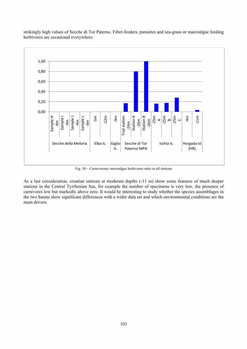
103

strikingly high values of Secche di Tor Paterno. Filter-feeders, parasites and sea-grass or macroalgae feeding herbivores are occasional everywhere.

Fig. 30 – Carnivorous/ microalgae herbivores ratio in all stations

As a last consideration, croatian stations at moderate depths (-11 m) show some features of much deeper stations in the Central Tyrrhenian Sea, for example the number of specimens is very low, the presence of carnivores low but markedly above zero. It would be interesting to study whether the species assemblages in the two basins show significant differences with a wider data set and which environmental conditions are the main drivers.

0,00

0,20

0,40

0,60

0,80

1,00

Sample H 

‐4m

Sample I

‐4m

Sample J

‐4m

Sample L 

‐4m ‐5m

‐12m ‐9m

Trial statio

n‐24m

Station 6

‐26m

Station 8

‐26m ‐25m

 A

‐25m

 B

‐25m

 C ‐4m

‐11m

Secche della Meloria Elba Is. Giglio Is.

Secche di Tor Paterno MPA

Ischia Is. Hvrgada Isl (HR)

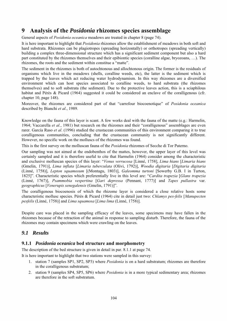
104

9 Analysis of the Posidonia rhizomes species assemblage General aspects of Posidonia oceanica meadows are treated in chapter 8 (page 74). It is here important to highlight that Posidonia rhizomes allow the establishment of meadows in both soft and hard substrata. Rhizomes can be plagiotropes (spreading horizontally) or orthotropes (spreading vertically) building a complex three-dimensional structure which has a significant sediment component but also a hard part constituted by the rhizomes themselves and their epibiontic species (coralline algae, bryozoans, …). The rhizomes, the roots and the sediment within constitue a “matte”. The sediment in the rhizomes is both of autochtonous and allochtonous origin. The former is the residuals of organisms which live in the meadows (shells, coralline weeds, etc), the latter is the sediment which is trapped by the leaves which act reducing water hydrodynamism. In this way rhizomes are a diversified environment which can host species associated to coralline weeds, to hard substrata (the rhizomes themselves) and to soft substrata (the sediment). Due to the protective leaves action, this is a sciaphilous habitat and Pérès & Picard (1964) suggested it could be considered an enclave of the coralligenous (cfr. chapter 10, page 148). Moreover, the rhizomes are considered part of that “carrefour biocoenotique” of Posidonia oceanica described by Bianchi et al., 1989. Knowledge on the fauna of this layer is scant. A few works deal with the fauna of the matte (e.g.: Harmelin, 1964; Vaccarella et al., 1981) but research on the rhizomes and their “coralligenous” assemblages are even rarer. García Raso et al. (1996) studied the crustacean communities of this environment comparing it to true coralligenous communities, concluding that the crustacean community is not significantly different. However, no specific work on the molluscs of the rhizomes was found. This is the first survey on the molluscan fauna of the Posidonia rhizomes of Secche di Tor Paterno. Our sampling was not aimed at the endobenthos of the mattes, however, the upper layer of this level was certainly sampled and it is therefore useful to cite that Harmelin (1964) consider among the characteristic and exclusive molluscan species of this layer: “Venus verrucosa [Linné, 1758], Lima hians [Limaria hians (Gmelin, 1791)], Lima inflata [Limaria tuberculata (Olivi, 1792)], Woodia digitaria [Digitaria digitaria (Linné, 1758)], Lepton squamosum [(Montagu, 1803)], Galeomma turtoni [Sowerby G.B. I in Turton, 1825]”. Characteristic species which preferentially live in this level are: “Cardita trapezia [Glans trapezia (Linné, 1767)], Psammobia vespertina [Gari depressa (Pennant, 1777)] and Tapes pullastra var. geographicus [Venerupis senegalensis (Gmelin, 1791)]”. The coralligenous biocoenosis of which the rhizome layer is considered a close relative hosts some characteristic mollusc species. Pérès & Picard (1964) cite in detail just two: Chlamys pes-felis [Manupecten pesfelis (Linné, 1758)] and Lima squamosa [Lima lima (Linné, 1758)]. Despite care was placed in the sampling efficacy of the leaves, some specimens may have fallen in the rhizomes because of the retraction of the animal in response to sampling disturb. Therefore, the fauna of the rhizomes may contain specimens which were crawling on the leaves.

9.1 Results

9.1.1 Posidonia oceanica bed structure and morphometry The description of the bed structure is given in detail in par. 8.1.1 at page 74. It is here important to highlight that two stations were sampled in this survey:

1. station 7 (samples SP1, SP2, SP3) where Posidonia is on a hard substratum; rhizomes are therefore in the coralligenous substratum;

2. station 9 (samples SP4, SP5, SP6) where Posidonia is in a more typical sedimentary area; rhizomes are therefore in the soft substratum.

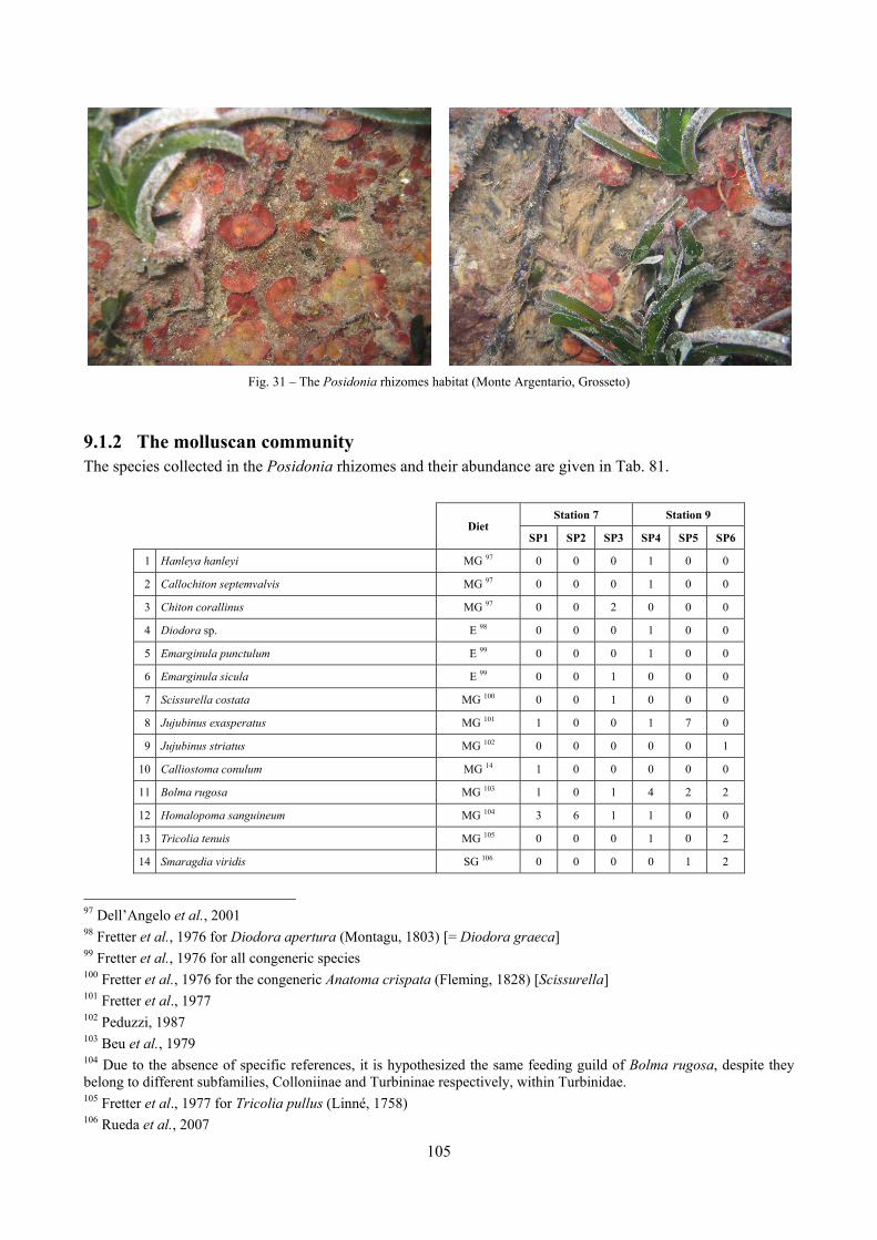
105

Fig. 31 – The Posidonia rhizomes habitat (Monte Argentario, Grosseto)

9.1.2 The molluscan community The species collected in the Posidonia rhizomes and their abundance are given in Tab. 81.

Diet Station 7 Station 9

SP1 SP2 SP3 SP4 SP5 SP6

1 Hanleya hanleyi MG 97 0 0 0 1 0 0

2 Callochiton septemvalvis MG 97 0 0 0 1 0 0

3 Chiton corallinus MG 97 0 0 2 0 0 0

4 Diodora sp. E 98 0 0 0 1 0 0

5 Emarginula punctulum E 99 0 0 0 1 0 0

6 Emarginula sicula E 99 0 0 1 0 0 0

7 Scissurella costata MG 100 0 0 1 0 0 0

8 Jujubinus exasperatus MG 101 1 0 0 1 7 0

9 Jujubinus striatus MG 102 0 0 0 0 0 1

10 Calliostoma conulum MG 14 1 0 0 0 0 0

11 Bolma rugosa MG 103 1 0 1 4 2 2

12 Homalopoma sanguineum MG 104 3 6 1 1 0 0

13 Tricolia tenuis MG 105 0 0 0 1 0 2

14 Smaragdia viridis SG 106 0 0 0 0 1 2

97 Dell’Angelo et al., 2001 98 Fretter et al., 1976 for Diodora apertura (Montagu, 1803) [= Diodora graeca] 99 Fretter et al., 1976 for all congeneric species 100 Fretter et al., 1976 for the congeneric Anatoma crispata (Fleming, 1828) [Scissurella] 101 Fretter et al., 1977 102 Peduzzi, 1987 103 Beu et al., 1979 104 Due to the absence of specific references, it is hypothesized the same feeding guild of Bolma rugosa, despite they belong to different subfamilies, Colloniinae and Turbininae respectively, within Turbinidae. 105 Fretter et al., 1977 for Tricolia pullus (Linné, 1758) 106 Rueda et al., 2007

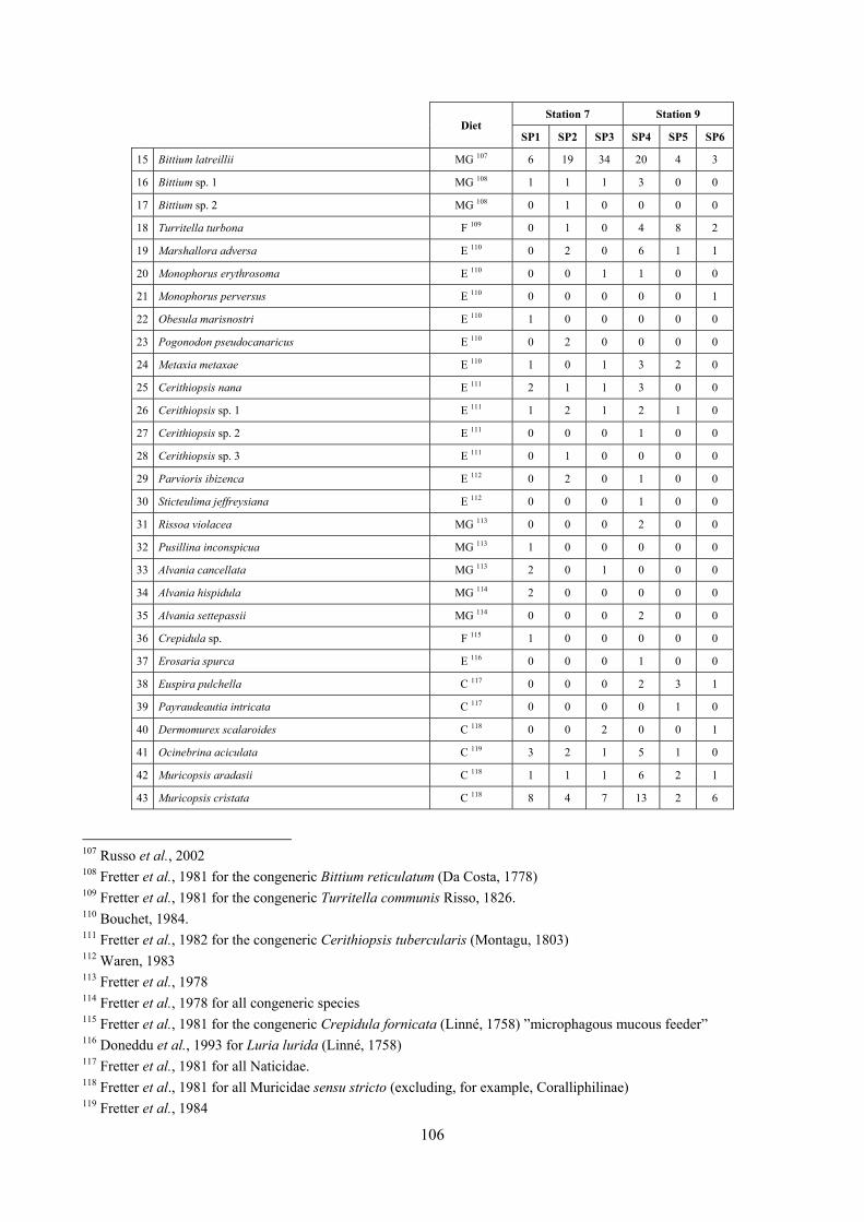
106

Diet Station 7 Station 9

SP1 SP2 SP3 SP4 SP5 SP6

15 Bittium latreillii MG 107 6 19 34 20 4 3

16 Bittium sp. 1 MG 108 1 1 1 3 0 0

17 Bittium sp. 2 MG 108 0 1 0 0 0 0

18 Turritella turbona F 109 0 1 0 4 8 2

19 Marshallora adversa E 110 0 2 0 6 1 1

20 Monophorus erythrosoma E 110 0 0 1 1 0 0

21 Monophorus perversus E 110 0 0 0 0 0 1

22 Obesula marisnostri E 110 1 0 0 0 0 0

23 Pogonodon pseudocanaricus E 110 0 2 0 0 0 0

24 Metaxia metaxae E 110 1 0 1 3 2 0

25 Cerithiopsis nana E 111 2 1 1 3 0 0

26 Cerithiopsis sp. 1 E 111 1 2 1 2 1 0

27 Cerithiopsis sp. 2 E 111 0 0 0 1 0 0

28 Cerithiopsis sp. 3 E 111 0 1 0 0 0 0

29 Parvioris ibizenca E 112 0 2 0 1 0 0

30 Sticteulima jeffreysiana E 112 0 0 0 1 0 0

31 Rissoa violacea MG 113 0 0 0 2 0 0

32 Pusillina inconspicua MG 113 1 0 0 0 0 0

33 Alvania cancellata MG 113 2 0 1 0 0 0

34 Alvania hispidula MG 114 2 0 0 0 0 0

35 Alvania settepassii MG 114 0 0 0 2 0 0

36 Crepidula sp. F 115 1 0 0 0 0 0

37 Erosaria spurca E 116 0 0 0 1 0 0

38 Euspira pulchella C 117 0 0 0 2 3 1

39 Payraudeautia intricata C 117 0 0 0 0 1 0

40 Dermomurex scalaroides C 118 0 0 2 0 0 1

41 Ocinebrina aciculata C 119 3 2 1 5 1 0

42 Muricopsis aradasii C 118 1 1 1 6 2 1

43 Muricopsis cristata C 118 8 4 7 13 2 6

107 Russo et al., 2002 108 Fretter et al., 1981 for the congeneric Bittium reticulatum (Da Costa, 1778) 109 Fretter et al., 1981 for the congeneric Turritella communis Risso, 1826. 110 Bouchet, 1984. 111 Fretter et al., 1982 for the congeneric Cerithiopsis tubercularis (Montagu, 1803) 112 Waren, 1983 113 Fretter et al., 1978 114 Fretter et al., 1978 for all congeneric species 115 Fretter et al., 1981 for the congeneric Crepidula fornicata (Linné, 1758) ”microphagous mucous feeder” 116 Doneddu et al., 1993 for Luria lurida (Linné, 1758) 117 Fretter et al., 1981 for all Naticidae. 118 Fretter et al., 1981 for all Muricidae sensu stricto (excluding, for example, Coralliphilinae) 119 Fretter et al., 1984

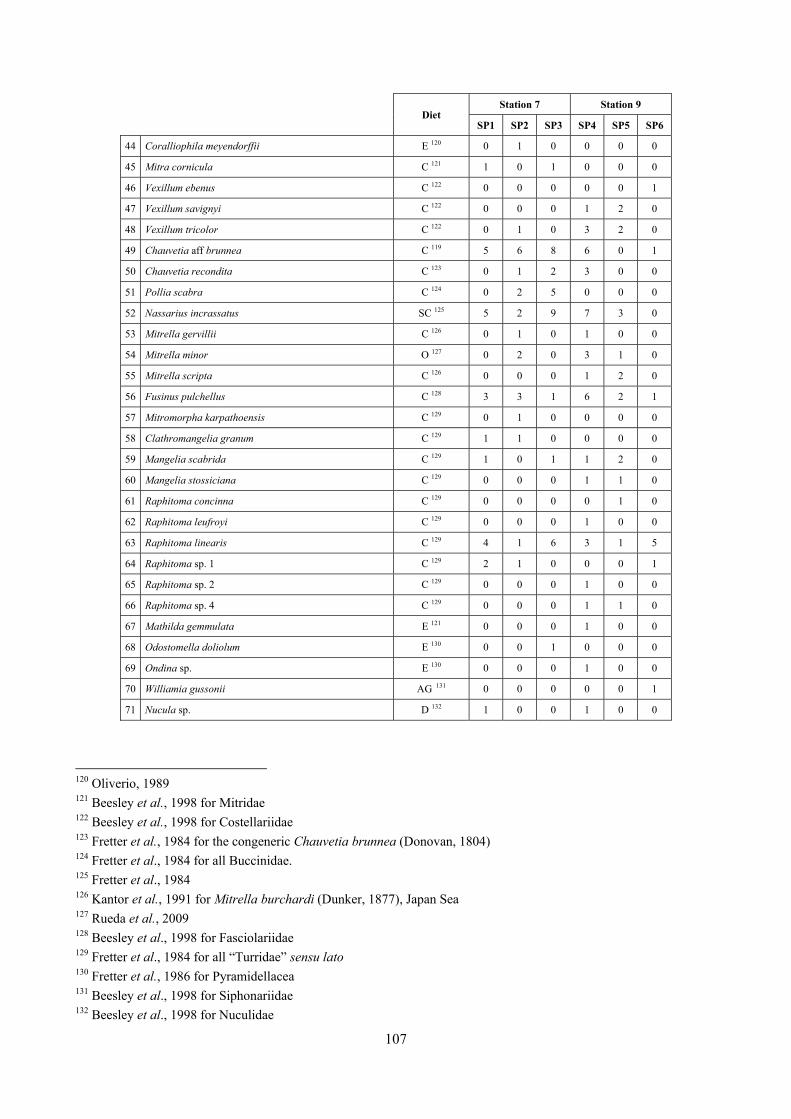
107

Diet Station 7 Station 9

SP1 SP2 SP3 SP4 SP5 SP6

44 Coralliophila meyendorffii E 120 0 1 0 0 0 0

45 Mitra cornicula C 121 1 0 1 0 0 0

46 Vexillum ebenus C 122 0 0 0 0 0 1

47 Vexillum savignyi C 122 0 0 0 1 2 0

48 Vexillum tricolor C 122 0 1 0 3 2 0

49 Chauvetia aff brunnea C 119 5 6 8 6 0 1

50 Chauvetia recondita C 123 0 1 2 3 0 0

51 Pollia scabra C 124 0 2 5 0 0 0

52 Nassarius incrassatus SC 125 5 2 9 7 3 0

53 Mitrella gervillii C 126 0 1 0 1 0 0

54 Mitrella minor O 127 0 2 0 3 1 0

55 Mitrella scripta C 126 0 0 0 1 2 0

56 Fusinus pulchellus C 128 3 3 1 6 2 1

57 Mitromorpha karpathoensis C 129 0 1 0 0 0 0

58 Clathromangelia granum C 129 1 1 0 0 0 0

59 Mangelia scabrida C 129 1 0 1 1 2 0

60 Mangelia stossiciana C 129 0 0 0 1 1 0

61 Raphitoma concinna C 129 0 0 0 0 1 0

62 Raphitoma leufroyi C 129 0 0 0 1 0 0

63 Raphitoma linearis C 129 4 1 6 3 1 5

64 Raphitoma sp. 1 C 129 2 1 0 0 0 1

65 Raphitoma sp. 2 C 129 0 0 0 1 0 0

66 Raphitoma sp. 4 C 129 0 0 0 1 1 0

67 Mathilda gemmulata E 121 0 0 0 1 0 0

68 Odostomella doliolum E 130 0 0 1 0 0 0

69 Ondina sp. E 130 0 0 0 1 0 0

70 Williamia gussonii AG 131 0 0 0 0 0 1

71 Nucula sp. D 132 1 0 0 1 0 0

120 Oliverio, 1989 121 Beesley et al., 1998 for Mitridae 122 Beesley et al., 1998 for Costellariidae 123 Fretter et al., 1984 for the congeneric Chauvetia brunnea (Donovan, 1804) 124 Fretter et al., 1984 for all Buccinidae. 125 Fretter et al., 1984 126 Kantor et al., 1991 for Mitrella burchardi (Dunker, 1877), Japan Sea 127 Rueda et al., 2009 128 Beesley et al., 1998 for Fasciolariidae 129 Fretter et al., 1984 for all “Turridae” sensu lato 130 Fretter et al., 1986 for Pyramidellacea 131 Beesley et al., 1998 for Siphonariidae 132 Beesley et al., 1998 for Nuculidae

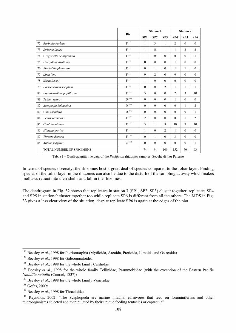
108

Diet Station 7 Station 9

SP1 SP2 SP3 SP4 SP5 SP6

72 Barbatia barbata F 133 1 3 1 2 0 0

73 Striarca lactea F 133 1 18 1 1 3 2

74 Gregariella semigranata F 133 1 0 0 0 0 1

75 Dacrydium hyalinum F 133 0 0 0 1 0 0

76 Modiolula phaseolina F 133 0 1 0 1 1 0

77 Lima lima F 133 0 2 0 0 0 0

78 Kurtiella sp. F 134 1 0 0 0 0 0

79 Parvicardium scriptum F 135 0 0 2 1 1 1

80 Papillicardium papillosum F 135 5 0 0 2 3 10

81 Tellina tenuis D 136 0 0 0 1 0 0

82 Arcopagia balaustina D 136 0 0 0 0 1 2

83 Gari costulata D 136 0 0 0 0 0 1

84 Venus verrucosa F 137 2 0 0 0 1 2

85 Gouldia minima F 137 3 1 3 10 7 10

86 Hiatella arctica F 138 1 0 2 1 0 0

87 Thracia distorta F 139 0 1 0 3 0 0

88 Antalis vulgaris C 140 0 0 0 0 0 1

TOTAL NUMBER OF SPECIMENS 74 94 100 152 70 63

Tab. 81 – Quali-quantitative data of the Posidonia rhizomes samples, Secche di Tor Paterno

In terms of species diversity, the rhizomes host a great deal of species compared to the foliar layer. Finding species of the foliar layer in the rhizomes can also be due to the disturb of the sampling activity which makes molluscs retract into their shells and fall in the rhizomes. The dendrogram in Fig. 32 shows that replicates in station 7 (SP1, SP2, SP3) cluster together, replicates SP4 and SP5 in station 9 cluster together too while replicate SP6 is different from all the others. The MDS in Fig. 33 gives a less clear view of the situation, despite replicate SP6 is again at the edges of the plot.

133 Beesley et al., 1998 for Pteriomorphia (Mytiloida, Arcoida, Pterioida, Limoida and Ostreoida) 134 Beesley et al., 1998 for Galeommatoidea 135 Beesley et al., 1998 for the whole family Cardiidae 136 Beesley et al., 1998 for the whole family Tellinidae, Psammobiidae (with the exception of the Eastern Pacific Nuttallia nuttallii (Conrad, 1837)) 137 Beesley et al., 1998 for the whole family Veneridae 138 Gofas, 2009a 139 Beesley et al., 1998 for Thracioidea 140 Reynolds, 2002: “The Scaphopoda are marine infaunal carnivores that feed on foraminiferans and other microorganisms selected and manipulated by their unique feeding tentacles or captacula”

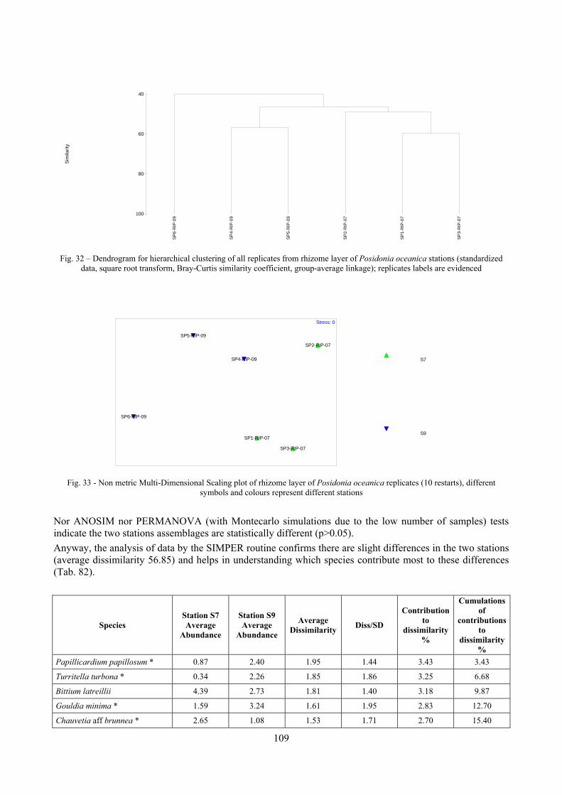
109

Fig. 32 – Dendrogram for hierarchical clustering of all replicates from rhizome layer of Posidonia oceanica stations (standardized

data, square root transform, Bray-Curtis similarity coefficient, group-average linkage); replicates labels are evidenced

Fig. 33 - Non metric Multi-Dimensional Scaling plot of rhizome layer of Posidonia oceanica replicates (10 restarts), different

symbols and colours represent different stations

Nor ANOSIM nor PERMANOVA (with Montecarlo simulations due to the low number of samples) tests indicate the two stations assemblages are statistically different (p>0.05). Anyway, the analysis of data by the SIMPER routine confirms there are slight differences in the two stations (average dissimilarity 56.85) and helps in understanding which species contribute most to these differences (Tab. 82).

Species Station S7 Average

Abundance

Station S9 Average

Abundance

Average Dissimilarity Diss/SD

Contribution to

dissimilarity %

Cumulations of

contributions to

dissimilarity%

Papillicardium papillosum * 0.87 2.40 1.95 1.44 3.43 3.43

Turritella turbona * 0.34 2.26 1.85 1.86 3.25 6.68

Bittium latreillii 4.39 2.73 1.81 1.40 3.18 9.87

Gouldia minima * 1.59 3.24 1.61 1.95 2.83 12.70

Chauvetia aff brunnea * 2.65 1.08 1.53 1.71 2.70 15.40

SP

6-R

IP-0

9

SP

4-R

IP-0

9

SP

5-R

IP-0

9

SP

2-R

IP-0

7

SP

1-R

IP-0

7

SP

3-R

IP-0

7

100

80

60

40

Sim

ilarit

y

S7

S9SP1-RIP-07

SP2-RIP-07

SP3-RIP-07

SP4-RIP-09

SP5-RIP-09

SP6-RIP-09

Stress: 0

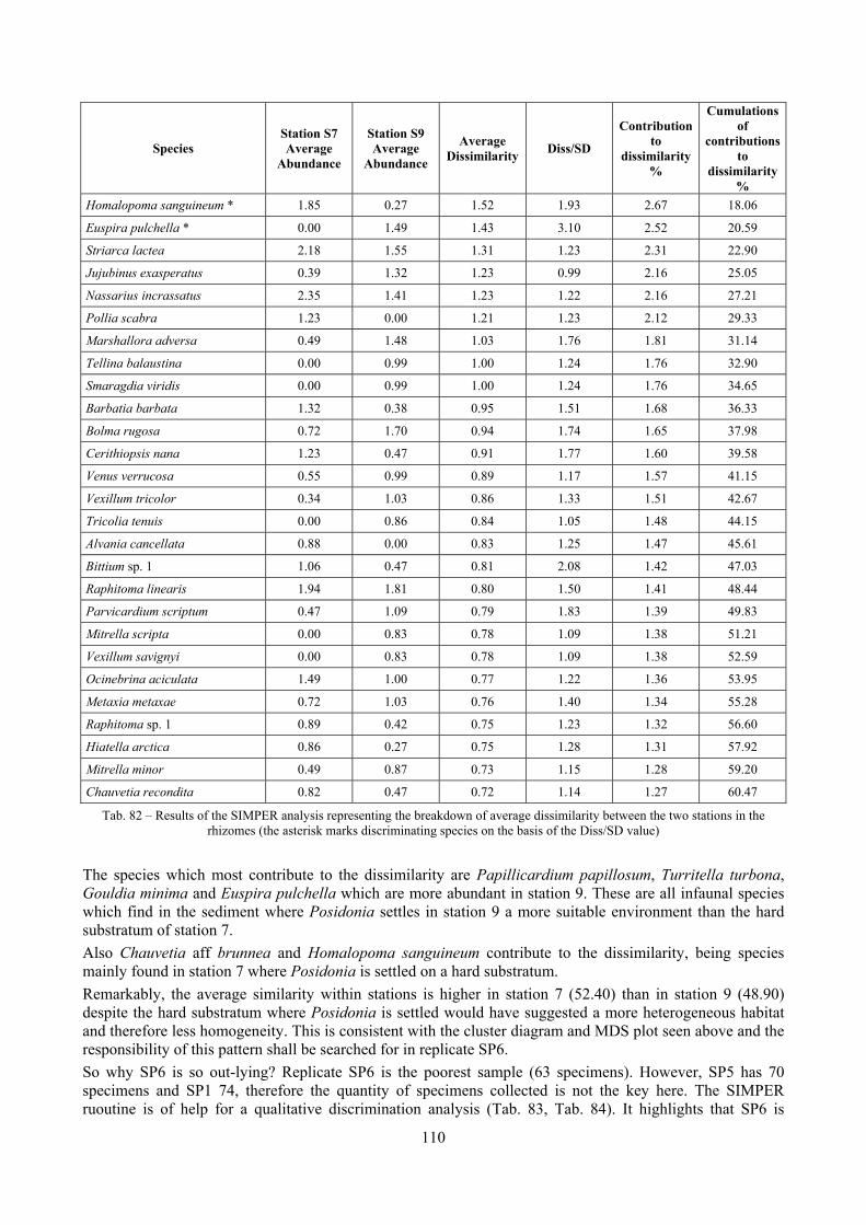
110

Species Station S7 Average

Abundance

Station S9 Average

Abundance

Average Dissimilarity Diss/SD

Contribution to

dissimilarity %

Cumulations of

contributions to

dissimilarity%

Homalopoma sanguineum * 1.85 0.27 1.52 1.93 2.67 18.06

Euspira pulchella * 0.00 1.49 1.43 3.10 2.52 20.59

Striarca lactea 2.18 1.55 1.31 1.23 2.31 22.90

Jujubinus exasperatus 0.39 1.32 1.23 0.99 2.16 25.05

Nassarius incrassatus 2.35 1.41 1.23 1.22 2.16 27.21

Pollia scabra 1.23 0.00 1.21 1.23 2.12 29.33

Marshallora adversa 0.49 1.48 1.03 1.76 1.81 31.14

Tellina balaustina 0.00 0.99 1.00 1.24 1.76 32.90

Smaragdia viridis 0.00 0.99 1.00 1.24 1.76 34.65

Barbatia barbata 1.32 0.38 0.95 1.51 1.68 36.33

Bolma rugosa 0.72 1.70 0.94 1.74 1.65 37.98

Cerithiopsis nana 1.23 0.47 0.91 1.77 1.60 39.58

Venus verrucosa 0.55 0.99 0.89 1.17 1.57 41.15

Vexillum tricolor 0.34 1.03 0.86 1.33 1.51 42.67

Tricolia tenuis 0.00 0.86 0.84 1.05 1.48 44.15

Alvania cancellata 0.88 0.00 0.83 1.25 1.47 45.61

Bittium sp. 1 1.06 0.47 0.81 2.08 1.42 47.03

Raphitoma linearis 1.94 1.81 0.80 1.50 1.41 48.44

Parvicardium scriptum 0.47 1.09 0.79 1.83 1.39 49.83

Mitrella scripta 0.00 0.83 0.78 1.09 1.38 51.21

Vexillum savignyi 0.00 0.83 0.78 1.09 1.38 52.59

Ocinebrina aciculata 1.49 1.00 0.77 1.22 1.36 53.95

Metaxia metaxae 0.72 1.03 0.76 1.40 1.34 55.28

Raphitoma sp. 1 0.89 0.42 0.75 1.23 1.32 56.60

Hiatella arctica 0.86 0.27 0.75 1.28 1.31 57.92

Mitrella minor 0.49 0.87 0.73 1.15 1.28 59.20

Chauvetia recondita 0.82 0.47 0.72 1.14 1.27 60.47

Tab. 82 – Results of the SIMPER analysis representing the breakdown of average dissimilarity between the two stations in the rhizomes (the asterisk marks discriminating species on the basis of the Diss/SD value)

The species which most contribute to the dissimilarity are Papillicardium papillosum, Turritella turbona, Gouldia minima and Euspira pulchella which are more abundant in station 9. These are all infaunal species which find in the sediment where Posidonia settles in station 9 a more suitable environment than the hard substratum of station 7. Also Chauvetia aff brunnea and Homalopoma sanguineum contribute to the dissimilarity, being species mainly found in station 7 where Posidonia is settled on a hard substratum. Remarkably, the average similarity within stations is higher in station 7 (52.40) than in station 9 (48.90) despite the hard substratum where Posidonia is settled would have suggested a more heterogeneous habitat and therefore less homogeneity. This is consistent with the cluster diagram and MDS plot seen above and the responsibility of this pattern shall be searched for in replicate SP6. So why SP6 is so out-lying? Replicate SP6 is the poorest sample (63 specimens). However, SP5 has 70 specimens and SP1 74, therefore the quantity of specimens collected is not the key here. The SIMPER ruoutine is of help for a qualitative discrimination analysis (Tab. 83, Tab. 84). It highlights that SP6 is

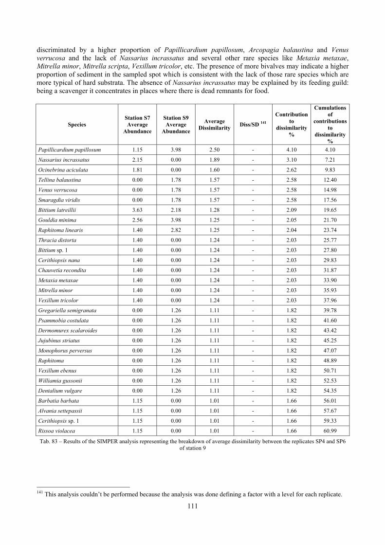
111

discriminated by a higher proportion of Papillicardium papillosum, Arcopagia balaustina and Venus verrucosa and the lack of Nassarius incrassatus and several other rare species like Metaxia metaxae, Mitrella minor, Mitrella scripta, Vexillum tricolor, etc. The presence of more bivalves may indicate a higher proportion of sediment in the sampled spot which is consistent with the lack of those rare species which are more typical of hard substrata. The absence of Nassarius incrassatus may be explained by its feeding guild: being a scavenger it concentrates in places where there is dead remnants for food.

Species Station S7 Average

Abundance

Station S9 Average

Abundance

Average Dissimilarity Diss/SD 141

Contribution to

dissimilarity %

Cumulations of

contributions to

dissimilarity%

Papillicardium papillosum 1.15 3.98 2.50 - 4.10 4.10

Nassarius incrassatus 2.15 0.00 1.89 - 3.10 7.21

Ocinebrina aciculata 1.81 0.00 1.60 - 2.62 9.83

Tellina balaustina 0.00 1.78 1.57 - 2.58 12.40

Venus verrucosa 0.00 1.78 1.57 - 2.58 14.98

Smaragdia viridis 0.00 1.78 1.57 - 2.58 17.56

Bittium latreillii 3.63 2.18 1.28 - 2.09 19.65

Gouldia minima 2.56 3.98 1.25 - 2.05 21.70

Raphitoma linearis 1.40 2.82 1.25 - 2.04 23.74

Thracia distorta 1.40 0.00 1.24 - 2.03 25.77

Bittium sp. 1 1.40 0.00 1.24 - 2.03 27.80

Cerithiopsis nana 1.40 0.00 1.24 - 2.03 29.83

Chauvetia recondita 1.40 0.00 1.24 - 2.03 31.87

Metaxia metaxae 1.40 0.00 1.24 - 2.03 33.90

Mitrella minor 1.40 0.00 1.24 - 2.03 35.93

Vexillum tricolor 1.40 0.00 1.24 - 2.03 37.96

Gregariella semigranata 0.00 1.26 1.11 - 1.82 39.78

Psammobia costulata 0.00 1.26 1.11 - 1.82 41.60

Dermomurex scalaroides 0.00 1.26 1.11 - 1.82 43.42

Jujubinus striatus 0.00 1.26 1.11 - 1.82 45.25

Monophorus perversus 0.00 1.26 1.11 - 1.82 47.07

Raphitoma 0.00 1.26 1.11 - 1.82 48.89

Vexillum ebenus 0.00 1.26 1.11 - 1.82 50.71

Williamia gussonii 0.00 1.26 1.11 - 1.82 52.53

Dentalium vulgare 0.00 1.26 1.11 - 1.82 54.35

Barbatia barbata 1.15 0.00 1.01 - 1.66 56.01

Alvania settepassii 1.15 0.00 1.01 - 1.66 57.67

Cerithiopsis sp. 1 1.15 0.00 1.01 - 1.66 59.33

Rissoa violacea 1.15 0.00 1.01 - 1.66 60.99

Tab. 83 – Results of the SIMPER analysis representing the breakdown of average dissimilarity between the replicates SP4 and SP6 of station 9

141 This analysis couldn’t be performed because the analysis was done defining a factor with a level for each replicate.

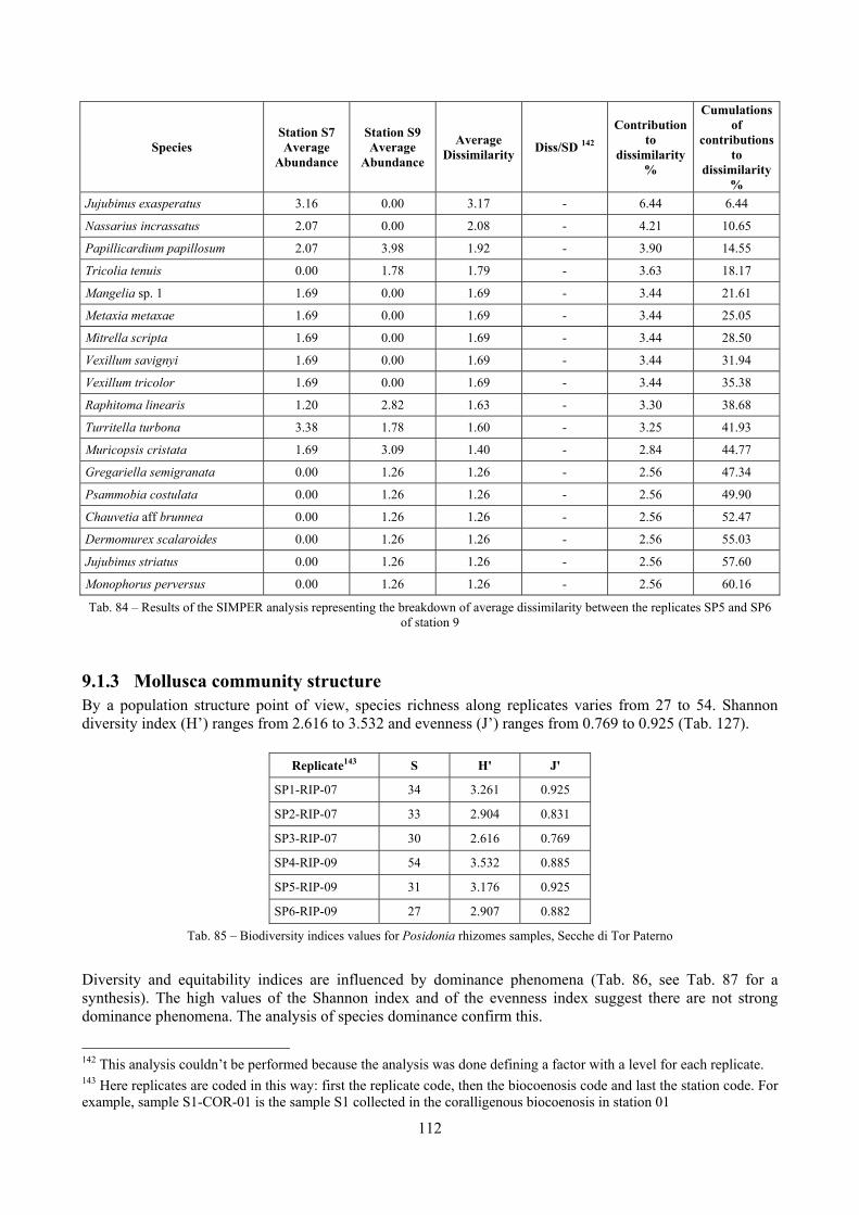
112

Species Station S7 Average

Abundance

Station S9 Average

Abundance

Average Dissimilarity Diss/SD 142

Contribution to

dissimilarity %

Cumulations of

contributions to

dissimilarity%

Jujubinus exasperatus 3.16 0.00 3.17 - 6.44 6.44

Nassarius incrassatus 2.07 0.00 2.08 - 4.21 10.65

Papillicardium papillosum 2.07 3.98 1.92 - 3.90 14.55

Tricolia tenuis 0.00 1.78 1.79 - 3.63 18.17

Mangelia sp. 1 1.69 0.00 1.69 - 3.44 21.61

Metaxia metaxae 1.69 0.00 1.69 - 3.44 25.05

Mitrella scripta 1.69 0.00 1.69 - 3.44 28.50

Vexillum savignyi 1.69 0.00 1.69 - 3.44 31.94

Vexillum tricolor 1.69 0.00 1.69 - 3.44 35.38

Raphitoma linearis 1.20 2.82 1.63 - 3.30 38.68

Turritella turbona 3.38 1.78 1.60 - 3.25 41.93

Muricopsis cristata 1.69 3.09 1.40 - 2.84 44.77

Gregariella semigranata 0.00 1.26 1.26 - 2.56 47.34

Psammobia costulata 0.00 1.26 1.26 - 2.56 49.90

Chauvetia aff brunnea 0.00 1.26 1.26 - 2.56 52.47

Dermomurex scalaroides 0.00 1.26 1.26 - 2.56 55.03

Jujubinus striatus 0.00 1.26 1.26 - 2.56 57.60

Monophorus perversus 0.00 1.26 1.26 - 2.56 60.16

Tab. 84 – Results of the SIMPER analysis representing the breakdown of average dissimilarity between the replicates SP5 and SP6 of station 9

9.1.3 Mollusca community structure By a population structure point of view, species richness along replicates varies from 27 to 54. Shannon diversity index (H’) ranges from 2.616 to 3.532 and evenness (J’) ranges from 0.769 to 0.925 (Tab. 127).

Replicate143 S H' J'

SP1-RIP-07 34 3.261 0.925

SP2-RIP-07 33 2.904 0.831

SP3-RIP-07 30 2.616 0.769

SP4-RIP-09 54 3.532 0.885

SP5-RIP-09 31 3.176 0.925

SP6-RIP-09 27 2.907 0.882

Tab. 85 – Biodiversity indices values for Posidonia rhizomes samples, Secche di Tor Paterno

Diversity and equitability indices are influenced by dominance phenomena (Tab. 86, see Tab. 87 for a synthesis). The high values of the Shannon index and of the evenness index suggest there are not strong dominance phenomena. The analysis of species dominance confirm this.

142 This analysis couldn’t be performed because the analysis was done defining a factor with a level for each replicate. 143 Here replicates are coded in this way: first the replicate code, then the biocoenosis code and last the station code. For example, sample S1-COR-01 is the sample S1 collected in the coralligenous biocoenosis in station 01

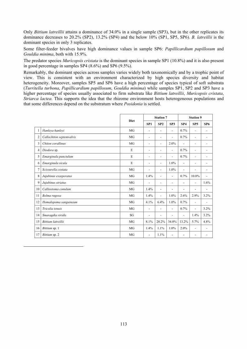
113

Only Bittium latreillii attains a dominance of 34.0% in a single sample (SP3), but in the other replicates its dominance decreases to 20.2% (SP2), 13.2% (SP4) and the below 10% (SP1, SP5, SP6). B. latreillii is the dominant species in only 3 replicates. Some filter-feeder bivalves have high dominance values in sample SP6: Papillicardium papillosum and Gouldia minima, both with 15.9%. The predator species Muricopsis cristata is the dominant species in sample SP1 (10.8%) and it is also present in good percentage in samples SP4 (8.6%) and SP6 (9.5%). Remarkably, the dominant species across samples varies widely both taxonomically and by a trophic point of view. This is consistent with an environment characterized by high species diversity and habitat heterogeneity. Moreover, samples SP5 and SP6 have a high percentage of species typical of soft substrata (Turritella turbona, Papillicardium papillosum, Gouldia minima) while samples SP1, SP2 and SP3 have a higher percentage of species usually associated to firm substrata like Bittium latreillii, Muricopsis cristata, Striarca lactea. This supports the idea that the rhizome environment hosts heterogeneous populations and that some differences depend on the substratum where Posidonia is settled.

Diet Station 7 Station 9

SP1 SP2 SP3 SP4 SP5 SP6

1 Hanleya hanleyi MG - - - 0.7% - -

2 Callochiton septemvalvis MG - - - 0.7% - -

3 Chiton corallinus MG - - 2.0% - - -

4 Diodora sp. E - - - 0.7% - -

5 Emarginula punctulum E - - - 0.7% - -

6 Emarginula sicula E - - 1.0% - - -

7 Scissurella costata MG - - 1.0% - - -

8 Jujubinus exasperatus MG 1.4% - - 0.7% 10.0% -

9 Jujubinus striatus MG - - - - - 1.6% 10 Calliostoma conulum MG 1.4% - - - - -

11 Bolma rugosa MG 1.4% - 1.0% 2.6% 2.9% 3.2%

12 Homalopoma sanguineum MG 4.1% 6.4% 1.0% 0.7% - -

13 Tricolia tenuis MG - - - 0.7% - 3.2%

14 Smaragdia viridis SG - - - - 1.4% 3.2%

15 Bittium latreillii MG 8.1% 20.2% 34.0% 13.2% 5.7% 4.8%

16 Bittium sp. 1 MG 1.4% 1.1% 1.0% 2.0% - -

17 Bittium sp. 2 MG - 1.1% - - - -

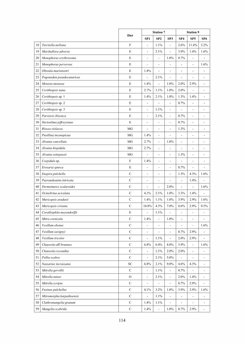
114

Diet Station 7 Station 9

SP1 SP2 SP3 SP4 SP5 SP6

18 Turritella turbona F - 1.1% - 2.6% 11.4% 3.2%

19 Marshallora adversa E - 2.1% - 3.9% 1.4% 1.6% 20 Monophorus erythrosoma E - - 1.0% 0.7% - -

21 Monophorus perversus E - - - - - 1.6% 22 Obesula marisnostri E 1.4% - - - - -

23 Pogonodon pseudocanaricus E - 2.1% - - - - 24 Metaxia metaxae E 1.4% - 1.0% 2.0% 2.9% -

25 Cerithiopsis nana E 2.7% 1.1% 1.0% 2.0% - - 26 Cerithiopsis sp. 1 E 1.4% 2.1% 1.0% 1.3% 1.4% -

27 Cerithiopsis sp. 2 E - - - 0.7% - -

28 Cerithiopsis sp. 3 E - 1.1% - - - -

29 Parvioris ibizenca E - 2.1% - 0.7% - - 30 Sticteulima jeffreysiana E - - - 0.7% - -

31 Rissoa violacea MG - - - 1.3% - -

32 Pusillina inconspicua MG 1.4% - - - - -

33 Alvania cancellata MG 2.7% - 1.0% - - -

34 Alvania hispidula MG 2.7% - - - - - 35 Alvania settepassii MG - - - 1.3% - -

36 Crepidula sp. F 1.4% - - - - -

37 Erosaria spurca E - - - 0.7% - -

38 Euspira pulchella C - - - 1.3% 4.3% 1.6% 39 Payraudeautia intricata C - - - - 1.4% -

40 Dermomurex scalaroides C - - 2.0% - - 1.6%

41 Ocinebrina aciculata C 4.1% 2.1% 1.0% 3.3% 1.4% - 42 Muricopsis aradasii C 1.4% 1.1% 1.0% 3.9% 2.9% 1.6% 43 Muricopsis cristata C 10.8% 4.3% 7.0% 8.6% 2.9% 9.5%

44 Coralliophila meyendorffii E - 1.1% - - - -

45 Mitra cornicula C 1.4% - 1.0% - - -

46 Vexillum ebenus C - - - - - 1.6% 47 Vexillum savignyi C - - - 0.7% 2.9% - 48 Vexillum tricolor C - 1.1% - 2.0% 2.9% - 49 Chauvetia aff brunnea C 6.8% 6.4% 8.0% 3.9% - 1.6%

50 Chauvetia recondita C - 1.1% 2.0% 2.0% - -

51 Pollia scabra C - 2.1% 5.0% - - -

52 Nassarius incrassatus SC 6.8% 2.1% 9.0% 4.6% 4.3% -

53 Mitrella gervillii C - 1.1% - 0.7% - -

54 Mitrella minor O - 2.1% - 2.0% 1.4% - 55 Mitrella scripta C - - - 0.7% 2.9% -

56 Fusinus pulchellus C 4.1% 3.2% 1.0% 3.9% 2.9% 1.6%

57 Mitromorpha karpathoensis C - 1.1% - - - -

58 Clathromangelia granum C 1.4% 1.1% - - - -

59 Mangelia scabrida C 1.4% - 1.0% 0.7% 2.9% -

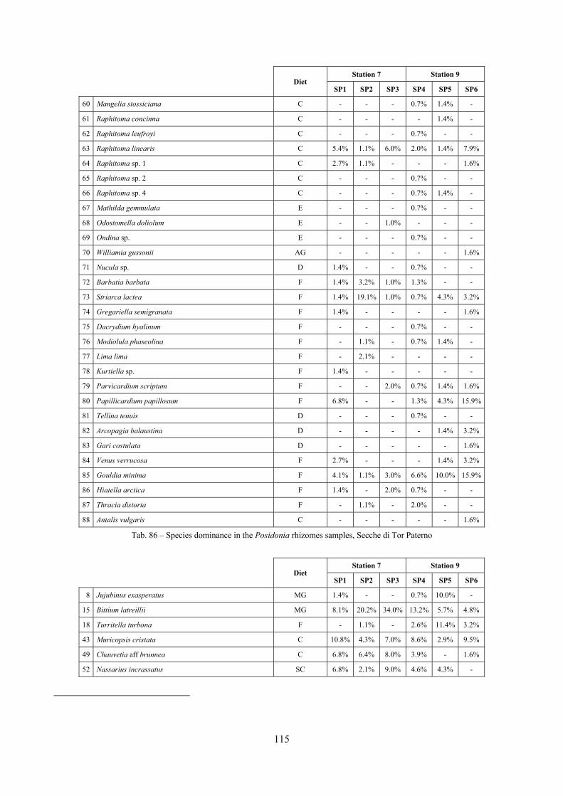
115

Diet Station 7 Station 9

SP1 SP2 SP3 SP4 SP5 SP6

60 Mangelia stossiciana C - - - 0.7% 1.4% -

61 Raphitoma concinna C - - - - 1.4% -

62 Raphitoma leufroyi C - - - 0.7% - -

63 Raphitoma linearis C 5.4% 1.1% 6.0% 2.0% 1.4% 7.9% 64 Raphitoma sp. 1 C 2.7% 1.1% - - - 1.6% 65 Raphitoma sp. 2 C - - - 0.7% - -

66 Raphitoma sp. 4 C - - - 0.7% 1.4% -

67 Mathilda gemmulata E - - - 0.7% - -

68 Odostomella doliolum E - - 1.0% - - -

69 Ondina sp. E - - - 0.7% - -

70 Williamia gussonii AG - - - - - 1.6%

71 Nucula sp. D 1.4% - - 0.7% - -

72 Barbatia barbata F 1.4% 3.2% 1.0% 1.3% - -

73 Striarca lactea F 1.4% 19.1% 1.0% 0.7% 4.3% 3.2% 74 Gregariella semigranata F 1.4% - - - - 1.6% 75 Dacrydium hyalinum F - - - 0.7% - - 76 Modiolula phaseolina F - 1.1% - 0.7% 1.4% -

77 Lima lima F - 2.1% - - - -

78 Kurtiella sp. F 1.4% - - - - -

79 Parvicardium scriptum F - - 2.0% 0.7% 1.4% 1.6% 80 Papillicardium papillosum F 6.8% - - 1.3% 4.3% 15.9%

81 Tellina tenuis D - - - 0.7% - -

82 Arcopagia balaustina D - - - - 1.4% 3.2% 83 Gari costulata D - - - - - 1.6%

84 Venus verrucosa F 2.7% - - - 1.4% 3.2% 85 Gouldia minima F 4.1% 1.1% 3.0% 6.6% 10.0% 15.9%

86 Hiatella arctica F 1.4% - 2.0% 0.7% - -

87 Thracia distorta F - 1.1% - 2.0% - -

88 Antalis vulgaris C - - - - - 1.6%

Tab. 86 – Species dominance in the Posidonia rhizomes samples, Secche di Tor Paterno

Diet

Station 7 Station 9

SP1 SP2 SP3 SP4 SP5 SP6

8 Jujubinus exasperatus MG 1.4% - - 0.7% 10.0% -

15 Bittium latreillii MG 8.1% 20.2% 34.0% 13.2% 5.7% 4.8%

18 Turritella turbona F - 1.1% - 2.6% 11.4% 3.2%

43 Muricopsis cristata C 10.8% 4.3% 7.0% 8.6% 2.9% 9.5%

49 Chauvetia aff brunnea C 6.8% 6.4% 8.0% 3.9% - 1.6%

52 Nassarius incrassatus SC 6.8% 2.1% 9.0% 4.6% 4.3% -

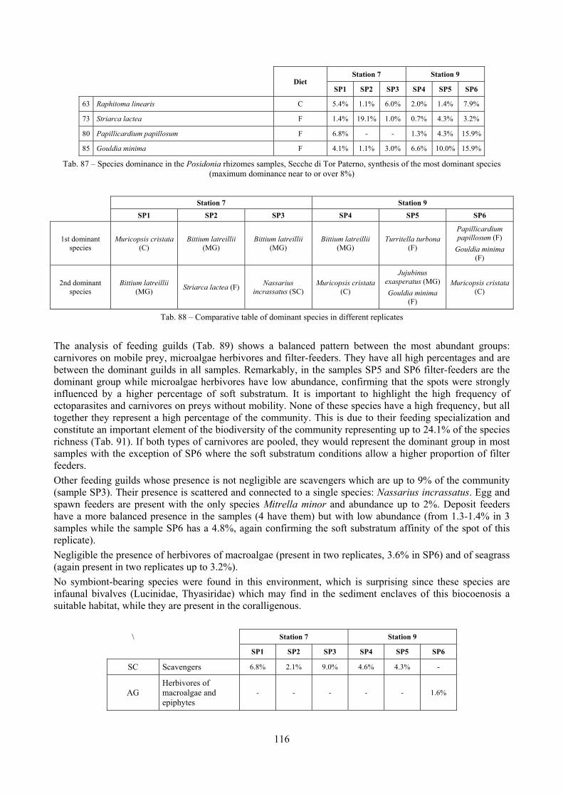
116

Diet Station 7 Station 9

SP1 SP2 SP3 SP4 SP5 SP6

63 Raphitoma linearis C 5.4% 1.1% 6.0% 2.0% 1.4% 7.9% 73 Striarca lactea F 1.4% 19.1% 1.0% 0.7% 4.3% 3.2% 80 Papillicardium papillosum F 6.8% - - 1.3% 4.3% 15.9%

85 Gouldia minima F 4.1% 1.1% 3.0% 6.6% 10.0% 15.9%

Tab. 87 – Species dominance in the Posidonia rhizomes samples, Secche di Tor Paterno, synthesis of the most dominant species (maximum dominance near to or over 8%)

Station 7 Station 9 SP1 SP2 SP3 SP4 SP5 SP6

1st dominant species

Muricopsis cristata (C)

Bittium latreillii (MG)

Bittium latreillii (MG)

Bittium latreillii (MG)

Turritella turbona (F)

Papillicardium papillosum (F)

Gouldia minima (F)

2nd dominant species

Bittium latreillii (MG) Striarca lactea (F) Nassarius

incrassatus (SC) Muricopsis cristata

(C)

Jujubinus exasperatus (MG) Gouldia minima

(F)

Muricopsis cristata (C)

Tab. 88 – Comparative table of dominant species in different replicates

The analysis of feeding guilds (Tab. 89) shows a balanced pattern between the most abundant groups: carnivores on mobile prey, microalgae herbivores and filter-feeders. They have all high percentages and are between the dominant guilds in all samples. Remarkably, in the samples SP5 and SP6 filter-feeders are the dominant group while microalgae herbivores have low abundance, confirming that the spots were strongly influenced by a higher percentage of soft substratum. It is important to highlight the high frequency of ectoparasites and carnivores on preys without mobility. None of these species have a high frequency, but all together they represent a high percentage of the community. This is due to their feeding specialization and constitute an important element of the biodiversity of the community representing up to 24.1% of the species richness (Tab. 91). If both types of carnivores are pooled, they would represent the dominant group in most samples with the exception of SP6 where the soft substratum conditions allow a higher proportion of filter feeders. Other feeding guilds whose presence is not negligible are scavengers which are up to 9% of the community (sample SP3). Their presence is scattered and connected to a single species: Nassarius incrassatus. Egg and spawn feeders are present with the only species Mitrella minor and abundance up to 2%. Deposit feeders have a more balanced presence in the samples (4 have them) but with low abundance (from 1.3-1.4% in 3 samples while the sample SP6 has a 4.8%, again confirming the soft substratum affinity of the spot of this replicate). Negligible the presence of herbivores of macroalgae (present in two replicates, 3.6% in SP6) and of seagrass (again present in two replicates up to 3.2%). No symbiont-bearing species were found in this environment, which is surprising since these species are infaunal bivalves (Lucinidae, Thyasiridae) which may find in the sediment enclaves of this biocoenosis a suitable habitat, while they are present in the coralligenous.

\

Station 7 Station 9

SP1 SP2 SP3 SP4 SP5 SP6

SC Scavengers 6.8% 2.1% 9.0% 4.6% 4.3% -

AG Herbivores of macroalgae and epiphytes

- - - - - 1.6%

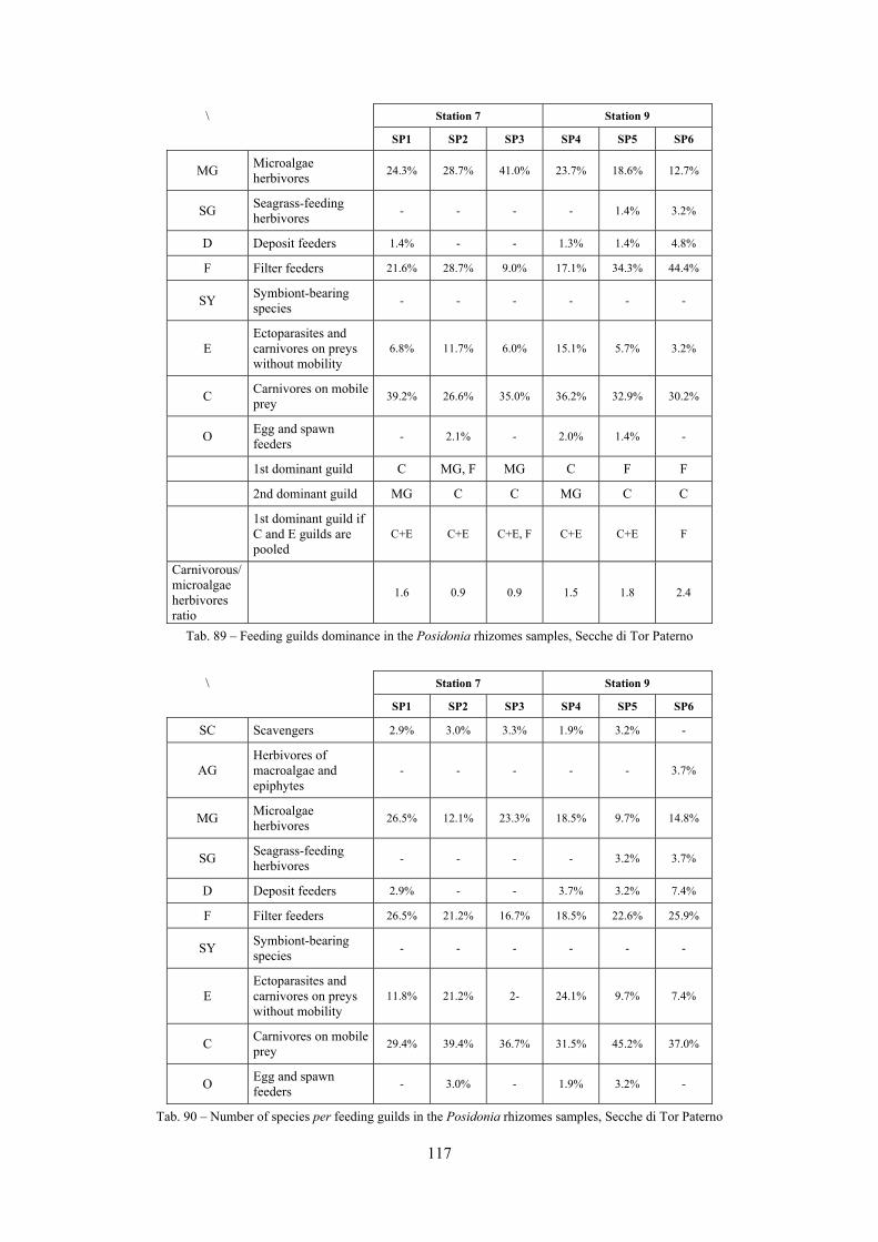
117

\

Station 7 Station 9

SP1 SP2 SP3 SP4 SP5 SP6

MG Microalgae herbivores 24.3% 28.7% 41.0% 23.7% 18.6% 12.7%

SG Seagrass-feeding herbivores - - - - 1.4% 3.2%

D Deposit feeders 1.4% - - 1.3% 1.4% 4.8%

F Filter feeders 21.6% 28.7% 9.0% 17.1% 34.3% 44.4%

SY Symbiont-bearing species - - - - - -

E Ectoparasites and carnivores on preys without mobility

6.8% 11.7% 6.0% 15.1% 5.7% 3.2%

C Carnivores on mobile prey 39.2% 26.6% 35.0% 36.2% 32.9% 30.2%

O Egg and spawn feeders - 2.1% - 2.0% 1.4% -

1st dominant guild C MG, F MG C F F

2nd dominant guild MG C C MG C C

1st dominant guild if C and E guilds are pooled

C+E C+E C+E, F C+E C+E F

Carnivorous/ microalgae herbivores ratio

1.6 0.9 0.9 1.5 1.8 2.4

Tab. 89 – Feeding guilds dominance in the Posidonia rhizomes samples, Secche di Tor Paterno

\

Station 7 Station 9

SP1 SP2 SP3 SP4 SP5 SP6

SC Scavengers 2.9% 3.0% 3.3% 1.9% 3.2% -

AG Herbivores of macroalgae and epiphytes

- - - - - 3.7%

MG Microalgae herbivores 26.5% 12.1% 23.3% 18.5% 9.7% 14.8%

SG Seagrass-feeding herbivores - - - - 3.2% 3.7%

D Deposit feeders 2.9% - - 3.7% 3.2% 7.4%

F Filter feeders 26.5% 21.2% 16.7% 18.5% 22.6% 25.9%

SY Symbiont-bearing species - - - - - -

E Ectoparasites and carnivores on preys without mobility

11.8% 21.2% 2- 24.1% 9.7% 7.4%

C Carnivores on mobile prey 29.4% 39.4% 36.7% 31.5% 45.2% 37.0%

O Egg and spawn feeders - 3.0% - 1.9% 3.2% -

Tab. 90 – Number of species per feeding guilds in the Posidonia rhizomes samples, Secche di Tor Paterno

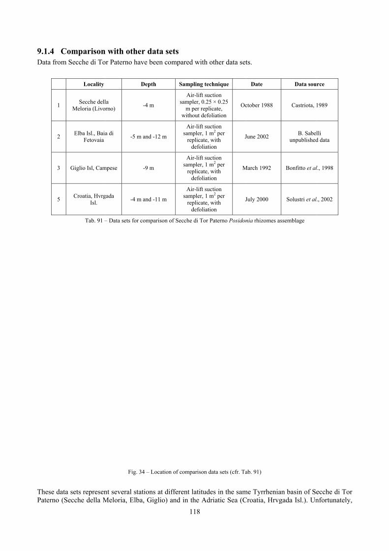
9.1.4 CoData from S

1

2

3

5

These data Paterno (Se

omparisonSecche di To

Locality

Secche dellMeloria (Livo

Elba Isl., BaiaFetovaia

Giglio Isl, Cam

Croatia, HvrgIsl.

Tab. 91 –

sets represenecche della M

with otheor Paterno ha

la rno)

a di -5 m

mpese

gada -4 m

– Data sets for c

Fig. 3

nt several staMeloria, Elba

er data setsve been com

Depth

-4 m

m and -12 m

-9 m

m and -11 m

comparison of S

34 – Location o

ations at diffea, Giglio) an

118

s mpared with o

Sampling tec

Air-lift sucsampler, 0.25

m per repliwithout defo

Air-lift sucsampler, 1 m

replicate, wdefoliati

Air-lift sucsampler, 1 m

replicate, wdefoliati

Air-lift sucsampler, 1 m

replicate, wdefoliati

Secche di Tor P

f comparison d

ferent latitudend in the Adr

other data set

chnique

ction 5 × 0.25 icate, oliation

Oc

ction m2 per with on

J

ction m2 per with on

M

ction m2 per with on

J

Paterno Posidon

data sets (cfr. Ta

es in the samriatic Sea (C

ts.

Date

ctober 1988

June 2002

March 1992

July 2000

nia rhizomes as

ab. 91)

me TyrrheniaCroatia, Hrvg

Data sou

Castriota,

B. Sabelunpublished

Bonfitto et al

Solustri et al

ssemblage

n basin of Segada Isl.). Un

rce

1989

lli d data

l., 1998

l., 2002

ecche di Tornfortunately,

r ,

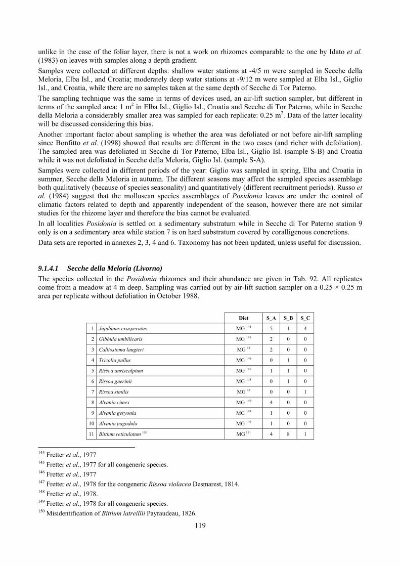
119

unlike in the case of the foliar layer, there is not a work on rhizomes comparable to the one by Idato et al. (1983) on leaves with samples along a depth gradient. Samples were collected at different depths: shallow water stations at -4/5 m were sampled in Secche della Meloria, Elba Isl., and Croatia; moderately deep water stations at -9/12 m were sampled at Elba Isl., Giglio Isl., and Croatia, while there are no samples taken at the same depth of Secche di Tor Paterno. The sampling technique was the same in terms of devices used, an air-lift suction sampler, but different in terms of the sampled area: 1 m2 in Elba Isl., Giglio Isl., Croatia and Secche di Tor Paterno, while in Secche della Meloria a considerably smaller area was sampled for each replicate: 0.25 m2. Data of the latter locality will be discussed considering this bias. Another important factor about sampling is whether the area was defoliated or not before air-lift sampling since Bonfitto et al. (1998) showed that results are different in the two cases (and richer with defoliation). The sampled area was defoliated in Secche di Tor Paterno, Elba Isl., Giglio Isl. (sample S-B) and Croatia while it was not defoliated in Secche della Meloria, Giglio Isl. (sample S-A). Samples were collected in different periods of the year: Giglio was sampled in spring, Elba and Croatia in summer, Secche della Meloria in autumn. The different seasons may affect the sampled species assemblage both qualitatively (because of species seasonality) and quantitatively (different recruitment periods). Russo et al. (1984) suggest that the molluscan species assemblages of Posidonia leaves are under the control of climatic factors related to depth and apparently independent of the season, however there are not similar studies for the rhizome layer and therefore the bias cannot be evaluated. In all localities Posidonia is settled on a sedimentary substratum while in Secche di Tor Paterno station 9 only is on a sedimentary area while station 7 is on hard substratum covered by coralligenous concretions. Data sets are reported in annexes 2, 3, 4 and 6. Taxonomy has not been updated, unless useful for discussion.

9.1.4.1 Secche della Meloria (Livorno) The species collected in the Posidonia rhizomes and their abundance are given in Tab. 92. All replicates come from a meadow at 4 m deep. Sampling was carried out by air-lift suction sampler on a 0.25 × 0.25 m area per replicate without defoliation in October 1988.

Diet S_A S_B S_C

1 Jujubinus exasperatus MG 144 5 1 4

2 Gibbula umbilicaris MG 145 2 0 0

3 Calliostoma laugieri MG 14 2 0 0

4 Tricolia pullus MG 146 0 1 0

5 Rissoa auriscalpium MG 147 1 1 0

6 Rissoa guerinii MG 148 0 1 0

7 Rissoa similis MG 47 0 0 1

8 Alvania cimex MG 149 4 0 0

9 Alvania geryonia MG 149 1 0 0

10 Alvania pagodula MG 149 1 0 0

11 Bittium reticulatum 150 MG 151 4 8 1

144 Fretter et al., 1977 145 Fretter et al., 1977 for all congeneric species. 146 Fretter et al., 1977 147 Fretter et al., 1978 for the congeneric Rissoa violacea Desmarest, 1814. 148 Fretter et al., 1978. 149 Fretter et al., 1978 for all congeneric species. 150 Misidentification of Bittium latreillii Payraudeau, 1826.

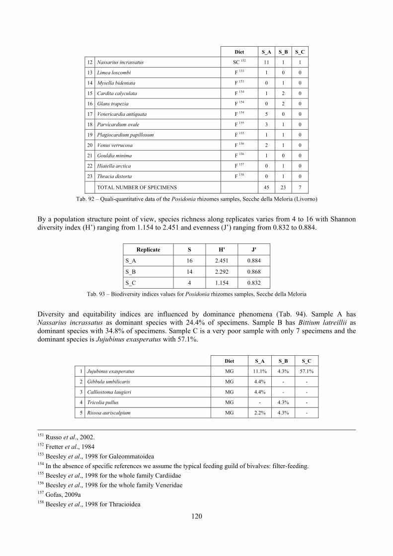
120

Diet S_A S_B S_C

12 Nassarius incrassatus SC 152 11 1 1

13 Limea loscombi F 133 1 0 0

14 Mysella bidentata F 153 0 1 0

15 Cardita calyculata F 154 1 2 0

16 Glans trapezia F 154 0 2 0

17 Venericardia antiquata F 154 5 0 0

18 Parvicardium ovale F 155 3 1 0

19 Plagiocardium papillosum F 155 1 1 0

20 Venus verrucosa F 156 2 1 0

21 Gouldia minima F 156 1 0 0

22 Hiatella arctica F 157 0 1 0

23 Thracia distorta F 158 0 1 0

TOTAL NUMBER OF SPECIMENS 45 23 7

Tab. 92 – Quali-quantitative data of the Posidonia rhizomes samples, Secche della Meloria (Livorno)

By a population structure point of view, species richness along replicates varies from 4 to 16 with Shannon diversity index (H’) ranging from 1.154 to 2.451 and evenness (J’) ranging from 0.832 to 0.884.

Replicate S H' J'

S_A 16 2.451 0.884

S_B 14 2.292 0.868

S_C 4 1.154 0.832

Tab. 93 – Biodiversity indices values for Posidonia rhizomes samples, Secche della Meloria

Diversity and equitability indices are influenced by dominance phenomena (Tab. 94). Sample A has Nassarius incrassatus as dominant species with 24.4% of specimens. Sample B has Bittium latreillii as dominant species with 34.8% of specimens. Sample C is a very poor sample with only 7 specimens and the dominant species is Jujubinus exasperatus with 57.1%.

Diet S_A S_B S_C

1 Jujubinus exasperatus MG 11.1% 4.3% 57.1%

2 Gibbula umbilicaris MG 4.4% - -

3 Calliostoma laugieri MG 4.4% - -

4 Tricolia pullus MG - 4.3% -

5 Rissoa auriscalpium MG 2.2% 4.3% -

151 Russo et al., 2002. 152 Fretter et al., 1984 153 Beesley et al., 1998 for Galeommatoidea 154 In the absence of specific references we assume the typical feeding guild of bivalves: filter-feeding. 155 Beesley et al., 1998 for the whole family Cardiidae 156 Beesley et al., 1998 for the whole family Veneridae 157 Gofas, 2009a 158 Beesley et al., 1998 for Thracioidea

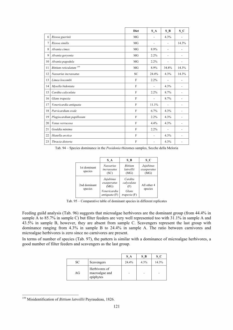
121

Diet S_A S_B S_C

6 Rissoa guerinii MG - 4.3% -

7 Rissoa similis MG - - 14.3%

8 Alvania cimex MG 8.9% - -

9 Alvania geryonia MG 2.2% - -

10 Alvania pagodula MG 2.2% - -

11 Bittium reticulatum 159 MG 8.9% 34.8% 14.3%

12 Nassarius incrassatus SC 24.4% 4.3% 14.3%

13 Limea loscombi F 2.2% - -

14 Mysella bidentata F - 4.3% -

15 Cardita calyculata F 2.2% 8.7% -

16 Glans trapezia F - 8.7% -

17 Venericardia antiquata F 11.1% - -

18 Parvicardium ovale F 6.7% 4.3% -

19 Plagiocardium papillosum F 2.2% 4.3% -

20 Venus verrucosa F 4.4% 4.3% -

21 Gouldia minima F 2.2% - -

22 Hiatella arctica F - 4.3% -

23 Thracia distorta F - 4.3% -

Tab. 94 – Species dominance in the Posidonia rhizomes samples, Secche della Meloria

S_A S_B S_C

1st dominant species

Nassarius incrassatus

(SC)

Bittium latreillii

(MG)

Jujubinus exasperatus

(MG)

2nd dominant species

Jujubinus exasperatus

(MG) Venericardia antiquata (F)

Cardita calyculata

(F) Glans

trapezia (F)

All other 4 species

Tab. 95 – Comparative table of dominant species in different replicates

Feeding guild analysis (Tab. 96) suggests that microalgae herbivores are the dominant group (from 44.4% in sample A to 85.7% in sample C) but filter feeders are very well represented too with 31.1% in sample A and 43.5% in sample B, however, they are absent from sample C. Scavengers represent the last group with dominance ranging from 4.3% in sample B to 24.4% in sample A. The ratio between carnivores and microalgae herbivores is zero since no carnivores are present. In terms of number of species (Tab. 97), the pattern is similar with a dominance of microalgae herbivores, a good number of filter feeders and scavengers as the last group.

S_A S_B S_C

SC Scavengers 24.4% 4.3% 14.3%

AG Herbivores of macroalgae and epiphytes

- - -

159 Misidentification of Bittium latreillii Payraudeau, 1826.

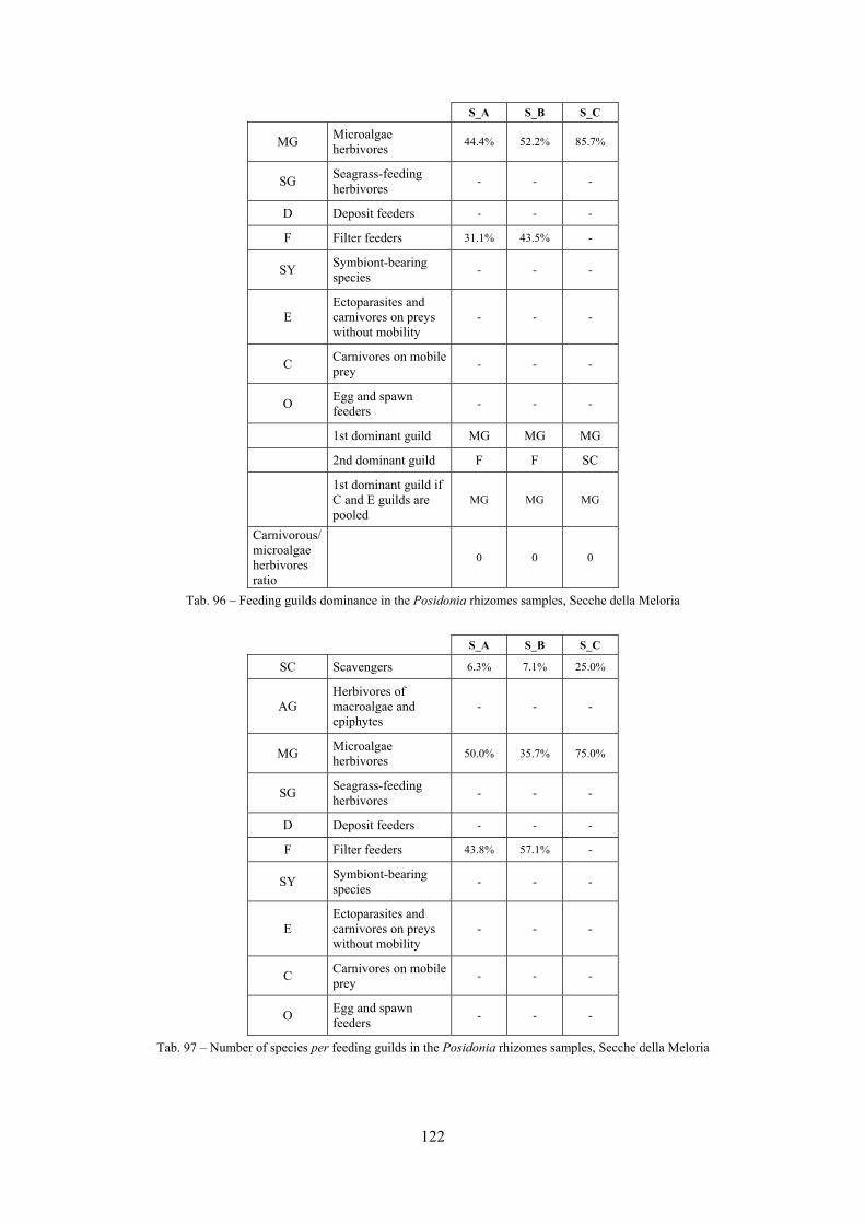
122

S_A S_B S_C

MG Microalgae herbivores 44.4% 52.2% 85.7%

SG Seagrass-feeding herbivores - - -

D Deposit feeders - - -

F Filter feeders 31.1% 43.5% -

SY Symbiont-bearing species - - -

E Ectoparasites and carnivores on preys without mobility

- - -

C Carnivores on mobile prey - - -

O Egg and spawn feeders - - -

1st dominant guild MG MG MG

2nd dominant guild F F SC

1st dominant guild if C and E guilds are pooled

MG MG MG

Carnivorous/ microalgae herbivores ratio

0 0 0

Tab. 96 – Feeding guilds dominance in the Posidonia rhizomes samples, Secche della Meloria

S_A S_B S_C

SC Scavengers 6.3% 7.1% 25.0%

AG Herbivores of macroalgae and epiphytes

- - -

MG Microalgae herbivores 50.0% 35.7% 75.0%

SG Seagrass-feeding herbivores - - -

D Deposit feeders - - -

F Filter feeders 43.8% 57.1% -

SY Symbiont-bearing species - - -

E Ectoparasites and carnivores on preys without mobility

- - -

C Carnivores on mobile prey - - -

O Egg and spawn feeders - - -

Tab. 97 – Number of species per feeding guilds in the Posidonia rhizomes samples, Secche della Meloria

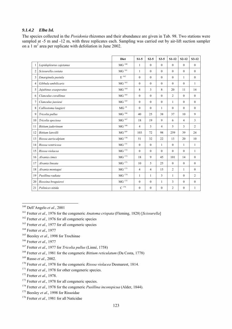
123

9.1.4.2 Elba Isl. The species collected in the Posidonia rhizomes and their abundance are given in Tab. 98. Two stations were sampled at -5 m and -12 m, with three replicates each. Sampling was carried out by air-lift suction sampler on a 1 m2 area per replicate with defoliation in June 2002.

Diet S1-5 S2-5 S3-5 S1-12 S2-12 S3-12

1 Lepidopleurus cajetanus MG 160 1 0 0 0 0 0

2 Scissurella costata MG 161 1 0 0 0 0 0

3 Emarginula pustula E 162 0 0 0 0 1 0

4 Gibbula umbilicaris MG 163 0 0 0 0 0 1

5 Jujubinus exasperatus MG 164 8 3 8 20 11 14

6 Clanculus corallinus MG 165 0 0 0 2 0 0

7 Clanculus jussieui MG 165 0 0 0 1 0 0

8 Calliostoma laugieri MG 14 0 0 1 0 0 0

9 Tricolia pullus MG 166 40 25 38 37 10 9

10 Tricolia speciosa MG 167 18 19 9 6 4 3

11 Bittium jadertinum MG 168 4 3 4 5 3 2

12 Bittium latreilli MG 169 103 72 98 259 39 24

13 Rissoa auriscalpium MG 170 51 32 22 13 20 10

14 Rissoa ventricosa MG 171 0 0 1 0 1 1

15 Rissoa violacea MG 172 0 0 0 0 0 1

16 Alvania cimex MG 173 18 9 45 101 14 0

17 Alvania lineata MG 173 10 5 25 0 0 0

18 Alvania montagui MG 173 4 4 15 2 1 0

19 Pusillina radiata MG 174 1 1 3 1 0 2

20 Rissoina bruguierei MG 175 0 0 1 3 0 0

21 Polinices nitida C 176 0 0 0 2 0 1

160 Dell’Angelo et al., 2001 161 Fretter et al., 1976 for the congeneric Anatoma crispata (Fleming, 1828) [Scissurella] 162 Fretter et al., 1976 for all congeneric species 163 Fretter et al., 1977 for all congeneric species 164 Fretter et al., 1977 165 Beesley et al., 1998 for Trochinae 166 Fretter et al., 1977 167 Fretter et al., 1977 for Tricolia pullus (Linné, 1758) 168 Fretter et al., 1981 for the congeneric Bittium reticulatum (Da Costa, 1778) 169 Russo et al., 2002. 170 Fretter et al., 1978 for the congeneric Rissoa violacea Desmarest, 1814. 171 Fretter et al., 1978 for other congeneric species. 172 Fretter et al., 1978. 173 Fretter et al., 1978 for all congeneric species. 174 Fretter et al., 1978 for the congeneric Pusillina inconspicua (Alder, 1844). 175 Beesley et al., 1998 for Rissoidae 176 Fretter et al., 1981 for all Naticidae

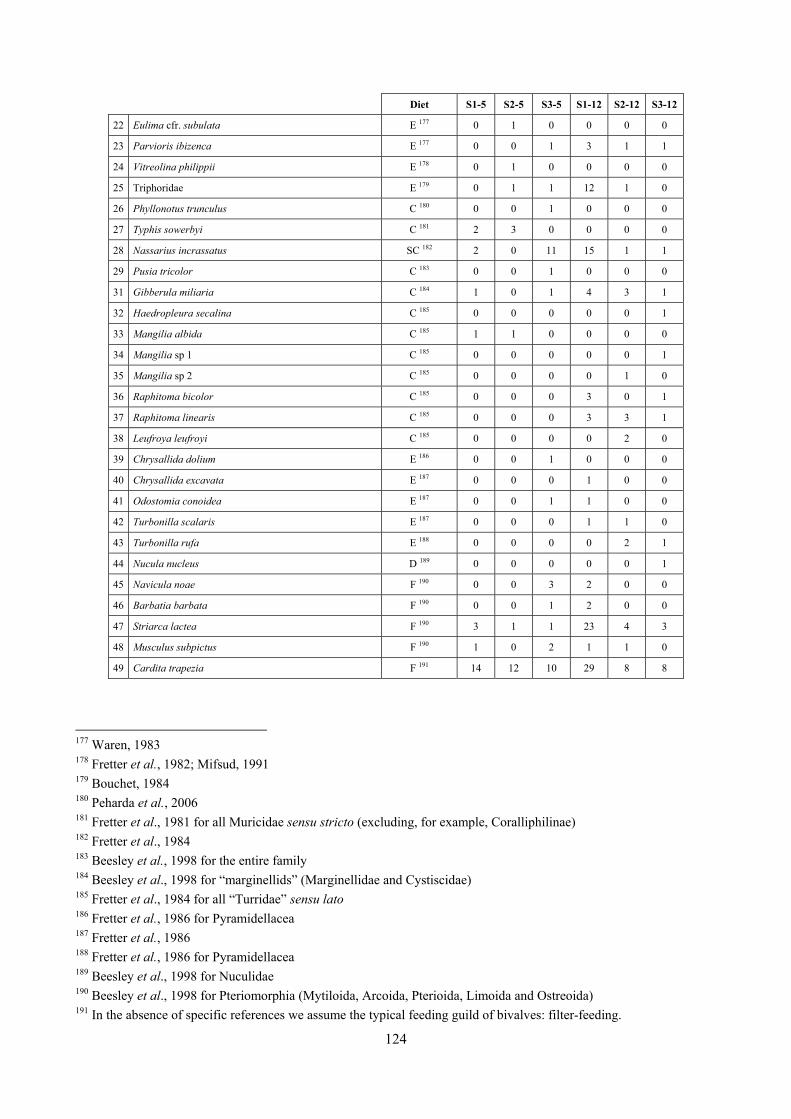
124

Diet S1-5 S2-5 S3-5 S1-12 S2-12 S3-12

22 Eulima cfr. subulata E 177 0 1 0 0 0 0

23 Parvioris ibizenca E 177 0 0 1 3 1 1

24 Vitreolina philippii E 178 0 1 0 0 0 0

25 Triphoridae E 179 0 1 1 12 1 0

26 Phyllonotus trunculus C 180 0 0 1 0 0 0

27 Typhis sowerbyi C 181 2 3 0 0 0 0

28 Nassarius incrassatus SC 182 2 0 11 15 1 1

29 Pusia tricolor C 183 0 0 1 0 0 0

31 Gibberula miliaria C 184 1 0 1 4 3 1

32 Haedropleura secalina C 185 0 0 0 0 0 1

33 Mangilia albida C 185 1 1 0 0 0 0

34 Mangilia sp 1 C 185 0 0 0 0 0 1

35 Mangilia sp 2 C 185 0 0 0 0 1 0

36 Raphitoma bicolor C 185 0 0 0 3 0 1

37 Raphitoma linearis C 185 0 0 0 3 3 1

38 Leufroya leufroyi C 185 0 0 0 0 2 0

39 Chrysallida dolium E 186 0 0 1 0 0 0

40 Chrysallida excavata E 187 0 0 0 1 0 0

41 Odostomia conoidea E 187 0 0 1 1 0 0

42 Turbonilla scalaris E 187 0 0 0 1 1 0

43 Turbonilla rufa E 188 0 0 0 0 2 1

44 Nucula nucleus D 189 0 0 0 0 0 1

45 Navicula noae F 190 0 0 3 2 0 0

46 Barbatia barbata F 190 0 0 1 2 0 0

47 Striarca lactea F 190 3 1 1 23 4 3

48 Musculus subpictus F 190 1 0 2 1 1 0

49 Cardita trapezia F 191 14 12 10 29 8 8

177 Waren, 1983 178 Fretter et al., 1982; Mifsud, 1991 179 Bouchet, 1984 180 Peharda et al., 2006 181 Fretter et al., 1981 for all Muricidae sensu stricto (excluding, for example, Coralliphilinae) 182 Fretter et al., 1984 183 Beesley et al., 1998 for the entire family 184 Beesley et al., 1998 for “marginellids” (Marginellidae and Cystiscidae) 185 Fretter et al., 1984 for all “Turridae” sensu lato 186 Fretter et al., 1986 for Pyramidellacea 187 Fretter et al., 1986 188 Fretter et al., 1986 for Pyramidellacea 189 Beesley et al., 1998 for Nuculidae 190 Beesley et al., 1998 for Pteriomorphia (Mytiloida, Arcoida, Pterioida, Limoida and Ostreoida) 191 In the absence of specific references we assume the typical feeding guild of bivalves: filter-feeding.

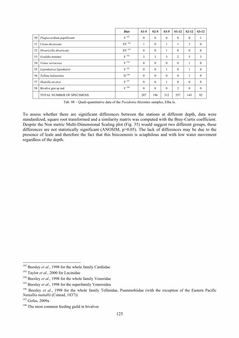
125

Diet S1-5 S2-5 S3-5 S1-12 S2-12 S3-12

50 Plagiocardium papillosum F 192 0 0 0 0 0 1

51 Ctena decussata SY 193 1 0 1 1 3 0

52 Divaricella divaricata SY 193 0 0 1 0 0 0

53 Gouldia minima F 194 3 3 3 2 5 3

54 Venus verrucosa F 194 0 0 0 0 1 0

55 Lajonkairea lajonkairii F 195 0 0 1 0 1 0

56 Tellina balaustina D 196 0 0 0 0 1 0

57 Hiatella arctica F 197 0 0 1 0 0 0

58 Bivalve gen sp ind F 198 0 0 0 2 0 0

TOTAL NUMBER OF SPECIMENS 287 196 312 557 143 92

Tab. 98 – Quali-quantitative data of the Posidonia rhizomes samples, Elba Is.

To assess whether there are significant differences between the stations at different depth, data were standardized, square root transformed and a similarity matrix was computed with the Bray-Curtis coefficient. Despite the Non metric Multi-Dimensional Scaling plot (Fig. 35) would suggest two different groups, these differences are not statistically significant (ANOSIM, p>0.05). The lack of differences may be due to the presence of leale and therefore the fact that this biocoenosis is sciaphilous and with low water movement regardless of the depth.

192 Beesley et al., 1998 for the whole family Cardiidae 193 Taylor et al., 2000 for Lucinidae 194 Beesley et al., 1998 for the whole family Veneridae 195 Beesley et al., 1998 for the superfamily Veneroidea 196 Beesley et al., 1998 for the whole family Tellinidae, Psammobiidae (with the exception of the Eastern Pacific Nuttallia nuttallii (Conrad, 1837)) 197 Gofas, 2009a 198 The most common feeding guild in bivalves

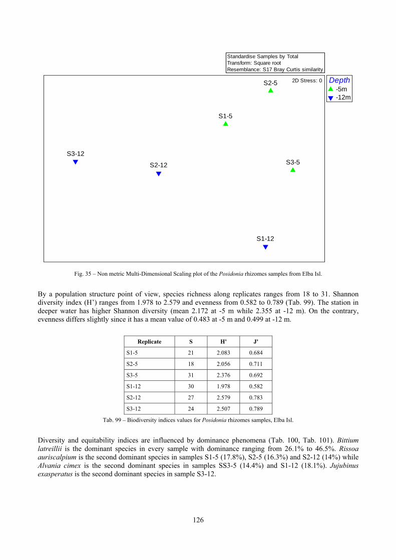
126

Fig. 35 – Non metric Multi-Dimensional Scaling plot of the Posidonia rhizomes samples from Elba Isl.

By a population structure point of view, species richness along replicates ranges from 18 to 31. Shannon diversity index (H’) ranges from 1.978 to 2.579 and evenness from 0.582 to 0.789 (Tab. 99). The station in deeper water has higher Shannon diversity (mean 2.172 at -5 m while 2.355 at -12 m). On the contrary, evenness differs slightly since it has a mean value of 0.483 at -5 m and 0.499 at -12 m.

Replicate S H' J'

S1-5 21 2.083 0.684

S2-5 18 2.056 0.711

S3-5 31 2.376 0.692

S1-12 30 1.978 0.582

S2-12 27 2.579 0.783

S3-12 24 2.507 0.789

Tab. 99 – Biodiversity indices values for Posidonia rhizomes samples, Elba Isl.

Diversity and equitability indices are influenced by dominance phenomena (Tab. 100, Tab. 101). Bittium latreillii is the dominant species in every sample with dominance ranging from 26.1% to 46.5%. Rissoa auriscalpium is the second dominant species in samples S1-5 (17.8%), S2-5 (16.3%) and S2-12 (14%) while Alvania cimex is the second dominant species in samples SS3-5 (14.4%) and S1-12 (18.1%). Jujubinus exasperatus is the second dominant species in sample S3-12.

Standardise Samples by TotalTransform: Square rootResemblance: S17 Bray Curtis similarity

Depth-5m-12m

S1-5

S2-5

S3-5

S1-12

S2-12

S3-12

2D Stress: 0

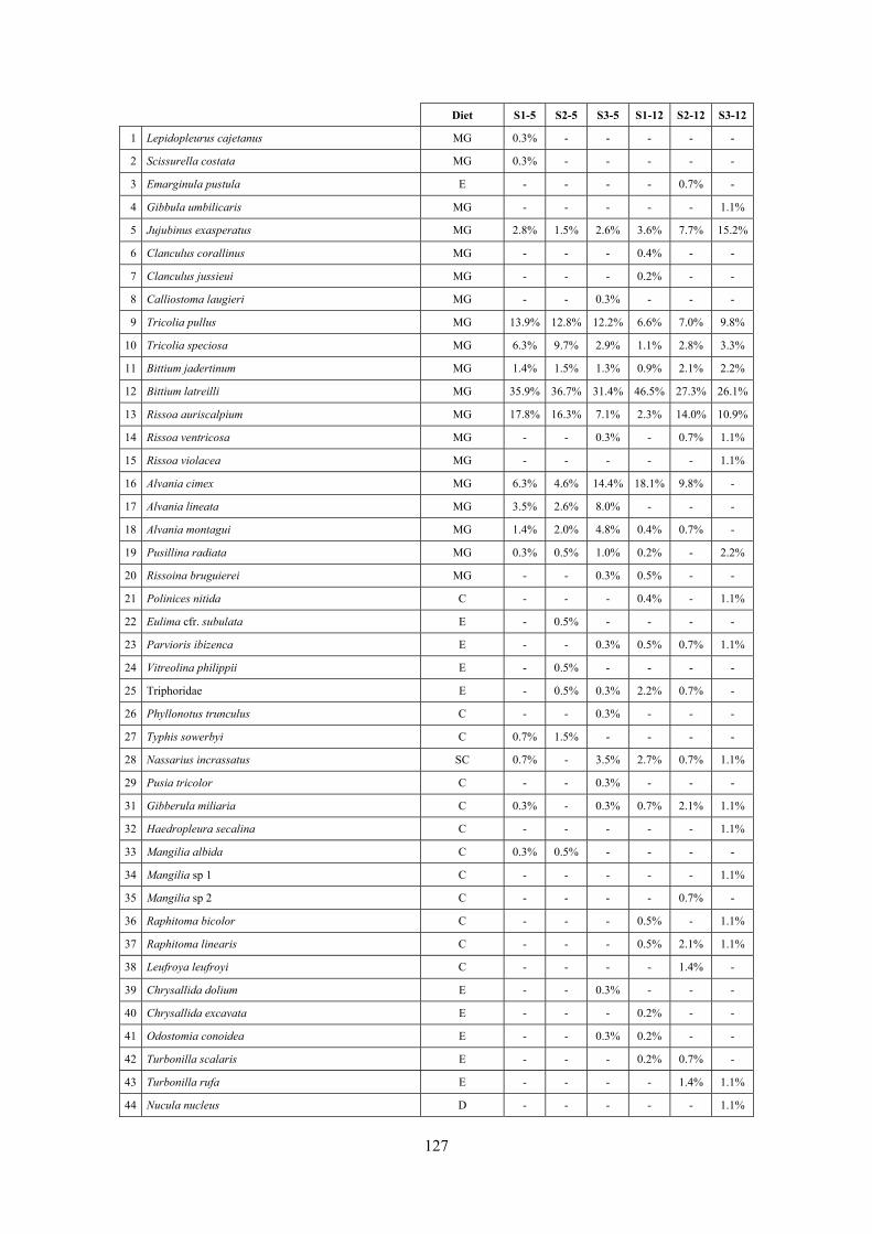
127

Diet S1-5 S2-5 S3-5 S1-12 S2-12 S3-12

1 Lepidopleurus cajetanus MG 0.3% - - - - -

2 Scissurella costata MG 0.3% - - - - -

3 Emarginula pustula E - - - - 0.7% -

4 Gibbula umbilicaris MG - - - - - 1.1%

5 Jujubinus exasperatus MG 2.8% 1.5% 2.6% 3.6% 7.7% 15.2%

6 Clanculus corallinus MG - - - 0.4% - -

7 Clanculus jussieui MG - - - 0.2% - -

8 Calliostoma laugieri MG - - 0.3% - - -

9 Tricolia pullus MG 13.9% 12.8% 12.2% 6.6% 7.0% 9.8%

10 Tricolia speciosa MG 6.3% 9.7% 2.9% 1.1% 2.8% 3.3%

11 Bittium jadertinum MG 1.4% 1.5% 1.3% 0.9% 2.1% 2.2%

12 Bittium latreilli MG 35.9% 36.7% 31.4% 46.5% 27.3% 26.1%

13 Rissoa auriscalpium MG 17.8% 16.3% 7.1% 2.3% 14.0% 10.9%

14 Rissoa ventricosa MG - - 0.3% - 0.7% 1.1%

15 Rissoa violacea MG - - - - - 1.1%

16 Alvania cimex MG 6.3% 4.6% 14.4% 18.1% 9.8% -

17 Alvania lineata MG 3.5% 2.6% 8.0% - - -

18 Alvania montagui MG 1.4% 2.0% 4.8% 0.4% 0.7% -

19 Pusillina radiata MG 0.3% 0.5% 1.0% 0.2% - 2.2%

20 Rissoina bruguierei MG - - 0.3% 0.5% - -

21 Polinices nitida C - - - 0.4% - 1.1%

22 Eulima cfr. subulata E - 0.5% - - - -

23 Parvioris ibizenca E - - 0.3% 0.5% 0.7% 1.1%

24 Vitreolina philippii E - 0.5% - - - -

25 Triphoridae E - 0.5% 0.3% 2.2% 0.7% -

26 Phyllonotus trunculus C - - 0.3% - - -

27 Typhis sowerbyi C 0.7% 1.5% - - - -

28 Nassarius incrassatus SC 0.7% - 3.5% 2.7% 0.7% 1.1%

29 Pusia tricolor C - - 0.3% - - -

31 Gibberula miliaria C 0.3% - 0.3% 0.7% 2.1% 1.1%

32 Haedropleura secalina C - - - - - 1.1%

33 Mangilia albida C 0.3% 0.5% - - - -

34 Mangilia sp 1 C - - - - - 1.1%

35 Mangilia sp 2 C - - - - 0.7% -

36 Raphitoma bicolor C - - - 0.5% - 1.1%

37 Raphitoma linearis C - - - 0.5% 2.1% 1.1%

38 Leufroya leufroyi C - - - - 1.4% -

39 Chrysallida dolium E - - 0.3% - - -

40 Chrysallida excavata E - - - 0.2% - -

41 Odostomia conoidea E - - 0.3% 0.2% - -

42 Turbonilla scalaris E - - - 0.2% 0.7% -

43 Turbonilla rufa E - - - - 1.4% 1.1%

44 Nucula nucleus D - - - - - 1.1%

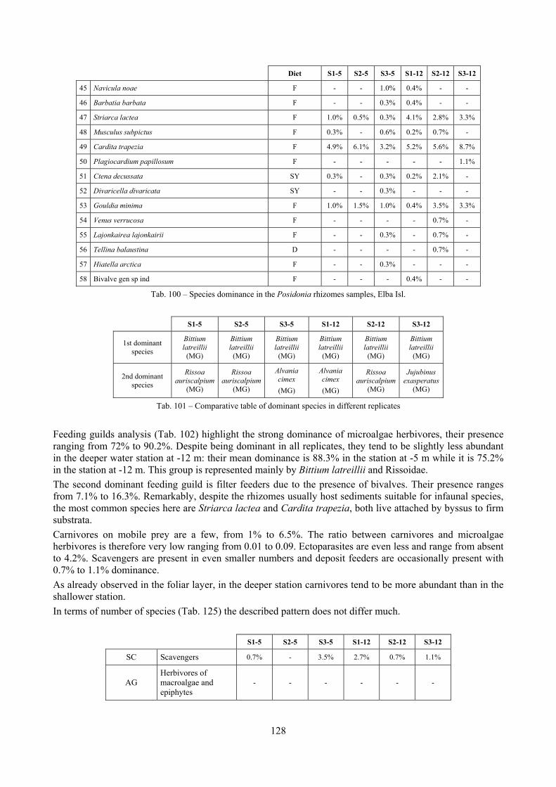
128

Diet S1-5 S2-5 S3-5 S1-12 S2-12 S3-12

45 Navicula noae F - - 1.0% 0.4% - -

46 Barbatia barbata F - - 0.3% 0.4% - -

47 Striarca lactea F 1.0% 0.5% 0.3% 4.1% 2.8% 3.3%

48 Musculus subpictus F 0.3% - 0.6% 0.2% 0.7% -

49 Cardita trapezia F 4.9% 6.1% 3.2% 5.2% 5.6% 8.7%

50 Plagiocardium papillosum F - - - - - 1.1%

51 Ctena decussata SY 0.3% - 0.3% 0.2% 2.1% -

52 Divaricella divaricata SY - - 0.3% - - -

53 Gouldia minima F 1.0% 1.5% 1.0% 0.4% 3.5% 3.3%

54 Venus verrucosa F - - - - 0.7% -

55 Lajonkairea lajonkairii F - - 0.3% - 0.7% -

56 Tellina balaustina D - - - - 0.7% -

57 Hiatella arctica F - - 0.3% - - -

58 Bivalve gen sp ind F - - - 0.4% - -

Tab. 100 – Species dominance in the Posidonia rhizomes samples, Elba Isl.

S1-5 S2-5 S3-5 S1-12 S2-12 S3-12

1st dominant species

Bittium latreillii

(MG)

Bittium latreillii

(MG)

Bittium latreillii

(MG)

Bittium latreillii

(MG)

Bittium latreillii

(MG)

Bittium latreillii

(MG)

2nd dominant species

Rissoa auriscalpium

(MG)

Rissoa auriscalpium

(MG)

Alvania cimex (MG)

Alvania cimex (MG)

Rissoa auriscalpium

(MG)

Jujubinus exasperatus

(MG)

Tab. 101 – Comparative table of dominant species in different replicates

Feeding guilds analysis (Tab. 102) highlight the strong dominance of microalgae herbivores, their presence ranging from 72% to 90.2%. Despite being dominant in all replicates, they tend to be slightly less abundant in the deeper water station at -12 m: their mean dominance is 88.3% in the station at -5 m while it is 75.2% in the station at -12 m. This group is represented mainly by Bittium latreillii and Rissoidae. The second dominant feeding guild is filter feeders due to the presence of bivalves. Their presence ranges from 7.1% to 16.3%. Remarkably, despite the rhizomes usually host sediments suitable for infaunal species, the most common species here are Striarca lactea and Cardita trapezia, both live attached by byssus to firm substrata. Carnivores on mobile prey are a few, from 1% to 6.5%. The ratio between carnivores and microalgae herbivores is therefore very low ranging from 0.01 to 0.09. Ectoparasites are even less and range from absent to 4.2%. Scavengers are present in even smaller numbers and deposit feeders are occasionally present with 0.7% to 1.1% dominance. As already observed in the foliar layer, in the deeper station carnivores tend to be more abundant than in the shallower station. In terms of number of species (Tab. 125) the described pattern does not differ much.

S1-5 S2-5 S3-5 S1-12 S2-12 S3-12

SC Scavengers 0.7% - 3.5% 2.7% 0.7% 1.1%

AG Herbivores of macroalgae and epiphytes

- - - - - -

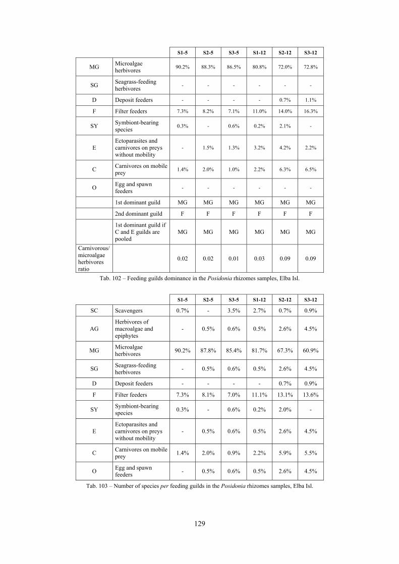
129

S1-5 S2-5 S3-5 S1-12 S2-12 S3-12

MG Microalgae herbivores 90.2% 88.3% 86.5% 80.8% 72.0% 72.8%

SG Seagrass-feeding herbivores - - - - - -

D Deposit feeders - - - - 0.7% 1.1%

F Filter feeders 7.3% 8.2% 7.1% 11.0% 14.0% 16.3%

SY Symbiont-bearing species 0.3% - 0.6% 0.2% 2.1% -

E Ectoparasites and carnivores on preys without mobility

- 1.5% 1.3% 3.2% 4.2% 2.2%

C Carnivores on mobile prey 1.4% 2.0% 1.0% 2.2% 6.3% 6.5%

O Egg and spawn feeders - - - - - -

1st dominant guild MG MG MG MG MG MG

2nd dominant guild F F F F F F

1st dominant guild if C and E guilds are pooled

MG MG MG MG MG MG

Carnivorous/ microalgae herbivores ratio

0.02 0.02 0.01 0.03 0.09 0.09

Tab. 102 – Feeding guilds dominance in the Posidonia rhizomes samples, Elba Isl.

S1-5 S2-5 S3-5 S1-12 S2-12 S3-12

SC Scavengers 0.7% - 3.5% 2.7% 0.7% 0.9%

AG Herbivores of macroalgae and epiphytes

- 0.5% 0.6% 0.5% 2.6% 4.5%

MG Microalgae herbivores 90.2% 87.8% 85.4% 81.7% 67.3% 60.9%

SG Seagrass-feeding herbivores - 0.5% 0.6% 0.5% 2.6% 4.5%

D Deposit feeders - - - - 0.7% 0.9%

F Filter feeders 7.3% 8.1% 7.0% 11.1% 13.1% 13.6%

SY Symbiont-bearing species 0.3% - 0.6% 0.2% 2.0% -

E Ectoparasites and carnivores on preys without mobility

- 0.5% 0.6% 0.5% 2.6% 4.5%

C Carnivores on mobile prey 1.4% 2.0% 0.9% 2.2% 5.9% 5.5%

O Egg and spawn feeders - 0.5% 0.6% 0.5% 2.6% 4.5%

Tab. 103 – Number of species per feeding guilds in the Posidonia rhizomes samples, Elba Isl.

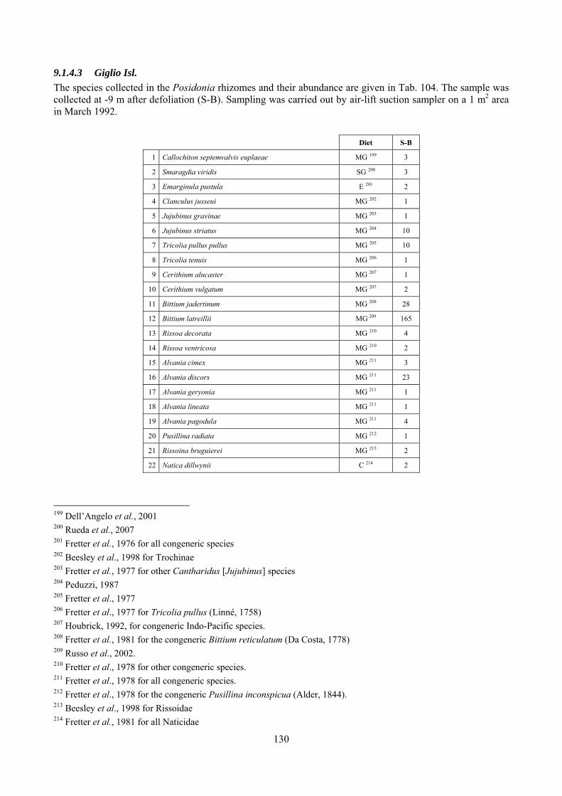
130

9.1.4.3 Giglio Isl. The species collected in the Posidonia rhizomes and their abundance are given in Tab. 104. The sample was collected at -9 m after defoliation (S-B). Sampling was carried out by air-lift suction sampler on a 1 m2 area in March 1992.

Diet S-B

1 Callochiton septemvalvis euplaeae MG 199 3

2 Smaragdia viridis SG 200 3

3 Emarginula pustula E 201 2

4 Clanculus jusseui MG 202 1

5 Jujubinus gravinae MG 203 1

6 Jujubinus striatus MG 204 10

7 Tricolia pullus pullus MG 205 10

8 Tricolia tenuis MG 206 1

9 Cerithium alucaster MG 207 1

10 Cerithium vulgatum MG 207 2

11 Bittium jadertinum MG 208 28

12 Bittium latreillii MG 209 165

13 Rissoa decorata MG 210 4

14 Rissoa ventricosa MG 210 2

15 Alvania cimex MG 211 3

16 Alvania discors MG 211 23

17 Alvania geryonia MG 211 1

18 Alvania lineata MG 211 1

19 Alvania pagodula MG 211 4

20 Pusillina radiata MG 212 1

21 Rissoina bruguierei MG 213 2

22 Natica dillwynii C 214 2

199 Dell’Angelo et al., 2001 200 Rueda et al., 2007 201 Fretter et al., 1976 for all congeneric species 202 Beesley et al., 1998 for Trochinae 203 Fretter et al., 1977 for other Cantharidus [Jujubinus] species 204 Peduzzi, 1987 205 Fretter et al., 1977 206 Fretter et al., 1977 for Tricolia pullus (Linné, 1758) 207 Houbrick, 1992, for congeneric Indo-Pacific species. 208 Fretter et al., 1981 for the congeneric Bittium reticulatum (Da Costa, 1778) 209 Russo et al., 2002. 210 Fretter et al., 1978 for other congeneric species. 211 Fretter et al., 1978 for all congeneric species. 212 Fretter et al., 1978 for the congeneric Pusillina inconspicua (Alder, 1844). 213 Beesley et al., 1998 for Rissoidae 214 Fretter et al., 1981 for all Naticidae

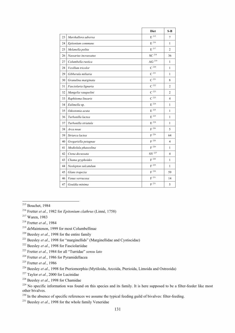
131

Diet S-B

23 Marshallora adversa E 215 7

24 Epitonium commune E 216 1

25 Melanella polita E 217 2

26 Nassarius incrassatus SC 218 36

27 Columbella rustica AG 219 1

28 Vexillum tricolor C 220 1

29 Gibberula miliaria C 221 1

30 Granulina marginata C 221 8

31 Fasciolaria lignaria C 222 2

32 Mangelia vauquelini C 223 2

33 Raphitoma linearis C 223 4

34 Eulimella sp. E 224 1

35 Odostomia acuta E 225 1

36 Turbonilla lactea E 225 1

37 Turbonilla striatula E 224 1

38 Arca noae F 226 5

39 Striarca lactea F 226 64

40 Gregariella petagnae F 226 4

41 Modiolula phaseolina F 226 1

42 Ctena decussata SY 227 4

43 Chama gryphoides F 228 1

44 Neolepton sulcatulum F 229 1

45 Glans trapezia F 230 59

46 Venus verrucosa F 231 14

47 Gouldia minima F 231 5

215 Bouchet, 1984 216 Fretter et al., 1982 for Epitonium clathrus (Linné, 1758) 217 Waren, 1983 218 Fretter et al., 1984 219 deMaintenon, 1999 for most Columbellinae 220 Beesley et al., 1998 for the entire family 221 Beesley et al., 1998 for “marginellids” (Marginellidae and Cystiscidae) 222 Beesley et al., 1998 for Fasciolariidae 223 Fretter et al., 1984 for all “Turridae” sensu lato 224 Fretter et al., 1986 for Pyramidellacea 225 Fretter et al., 1986 226 Beesley et al., 1998 for Pteriomorphia (Mytiloida, Arcoida, Pterioida, Limoida and Ostreoida) 227 Taylor et al., 2000 for Lucinidae 228 Beesley et al., 1998 for Chamidae 229 No specific information was found on this species and its family. It is here supposed to be a filter-feeder like most other bivalves. 230 In the absence of specific references we assume the typical feeding guild of bivalves: filter-feeding. 231 Beesley et al., 1998 for the whole family Veneridae

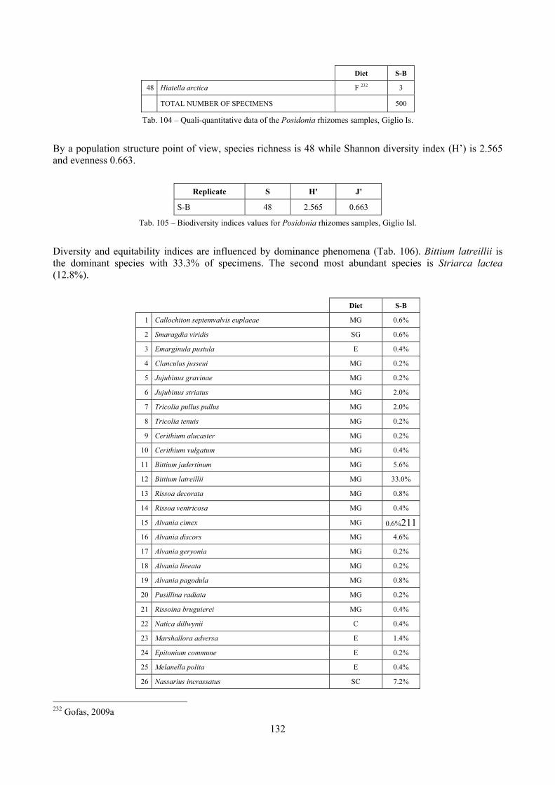
132

Diet S-B

48 Hiatella arctica F 232 3

TOTAL NUMBER OF SPECIMENS 500

Tab. 104 – Quali-quantitative data of the Posidonia rhizomes samples, Giglio Is.

By a population structure point of view, species richness is 48 while Shannon diversity index (H’) is 2.565 and evenness 0.663.

Replicate S H' J'

S-B 48 2.565 0.663

Tab. 105 – Biodiversity indices values for Posidonia rhizomes samples, Giglio Isl.

Diversity and equitability indices are influenced by dominance phenomena (Tab. 106). Bittium latreillii is the dominant species with 33.3% of specimens. The second most abundant species is Striarca lactea (12.8%).

Diet S-B

1 Callochiton septemvalvis euplaeae MG 0.6%

2 Smaragdia viridis SG 0.6%

3 Emarginula pustula E 0.4%

4 Clanculus jusseui MG 0.2%

5 Jujubinus gravinae MG 0.2%

6 Jujubinus striatus MG 2.0%

7 Tricolia pullus pullus MG 2.0%

8 Tricolia tenuis MG 0.2%

9 Cerithium alucaster MG 0.2%

10 Cerithium vulgatum MG 0.4%

11 Bittium jadertinum MG 5.6%

12 Bittium latreillii MG 33.0%

13 Rissoa decorata MG 0.8%

14 Rissoa ventricosa MG 0.4%

15 Alvania cimex MG 0.6%211

16 Alvania discors MG 4.6%

17 Alvania geryonia MG 0.2%

18 Alvania lineata MG 0.2%

19 Alvania pagodula MG 0.8%

20 Pusillina radiata MG 0.2%

21 Rissoina bruguierei MG 0.4%

22 Natica dillwynii C 0.4%

23 Marshallora adversa E 1.4%

24 Epitonium commune E 0.2%

25 Melanella polita E 0.4%

26 Nassarius incrassatus SC 7.2%

232 Gofas, 2009a

133

Diet S-B

27 Columbella rustica AG 0.2%

28 Vexillum tricolor C 0.2%

29 Gibberula miliaria C 0.2%

30 Granulina marginata C 1.6%

31 Fasciolaria lignaria C 0.4%

32 Mangelia vauquelini C 0.4%

33 Raphitoma linearis C 0.8%

34 Eulimella sp. E 0.2%

35 Odostomia acuta E 0.2%

36 Turbonilla lactea E 0.2%

37 Turbonilla striatula E 0.2%

38 Arca noae F 1.0%

39 Striarca lactea F 12.8%

40 Gregariella petagnae F 0.8%

41 Modiolula phaseolina F 0.2%

42 Ctena decussata SY 0.8%

43 Chama gryphoides F 0.2%

44 Neolepton sulcatulum F 0.2%

45 Glans trapezia F 11.8%

46 Venus verrucosa F 2.8%

47 Gouldia minima F 1.0%

48 Hiatella arctica F 0.6%

Tab. 106 – Species dominance in the Posidonia rhizomes samples, Giglio Isl.

S-B

1st dominant species

Bittium latreillii

(MG)

2nd dominant species

Striarca lactea (F)

Tab. 107 – Dominant species in the sample

Feeding guild analysis (Tab. 125) highlights the dominance of microalgae herbivores with 52.6%. Filter feeders are the second most abundant feeding guild (31.4%). Scavengers are the third group (7.2%) due to the abundant presence (36 specimens) of a single species (Nassarius incrassatus). Carnivores (4%) and ectoparasites (3.2%) are present in small numbers while herbivores on macroalgae are negligible. In terms of number of species (Tab. 109) the role of carnivores emerges being 14.6% of species. Ectoparasites are even more: 16.7%, accounting all together for 31.3% being the second most represented group. These samples had therefore a good species diversity of carnivores despite being rare species.

S-B

SC Scavengers 7.2%

AG Herbivores of macroalgae and epiphytes

0.2%

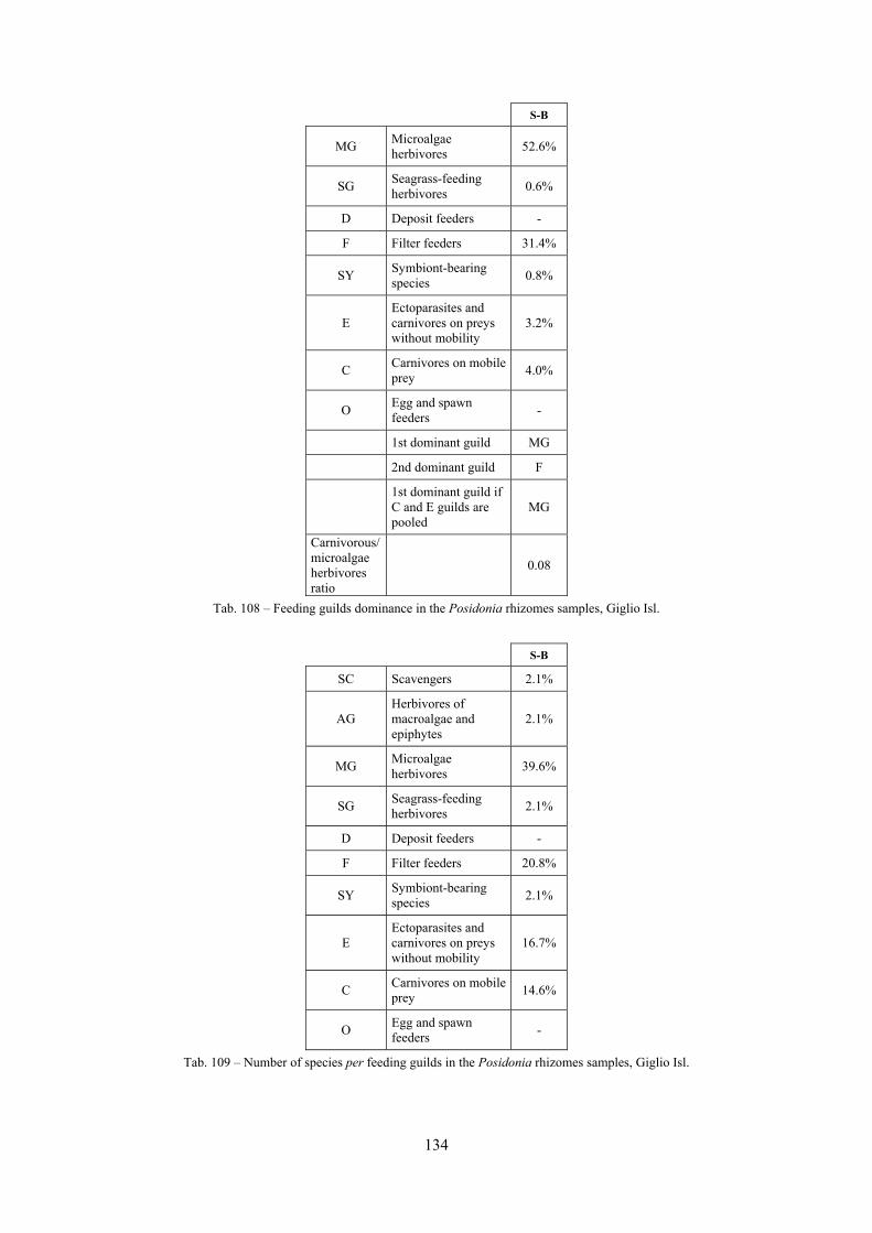
134

S-B

MG Microalgae herbivores 52.6%

SG Seagrass-feeding herbivores 0.6%

D Deposit feeders -

F Filter feeders 31.4%

SY Symbiont-bearing species 0.8%

E Ectoparasites and carnivores on preys without mobility

3.2%

C Carnivores on mobile prey 4.0%

O Egg and spawn feeders -

1st dominant guild MG

2nd dominant guild F

1st dominant guild if C and E guilds are pooled

MG

Carnivorous/ microalgae herbivores ratio

0.08

Tab. 108 – Feeding guilds dominance in the Posidonia rhizomes samples, Giglio Isl.

S-B

SC Scavengers 2.1%

AG Herbivores of macroalgae and epiphytes

2.1%

MG Microalgae herbivores 39.6%

SG Seagrass-feeding herbivores 2.1%

D Deposit feeders -

F Filter feeders 20.8%

SY Symbiont-bearing species 2.1%

E Ectoparasites and carnivores on preys without mobility

16.7%

C Carnivores on mobile prey 14.6%

O Egg and spawn feeders -

Tab. 109 – Number of species per feeding guilds in the Posidonia rhizomes samples, Giglio Isl.

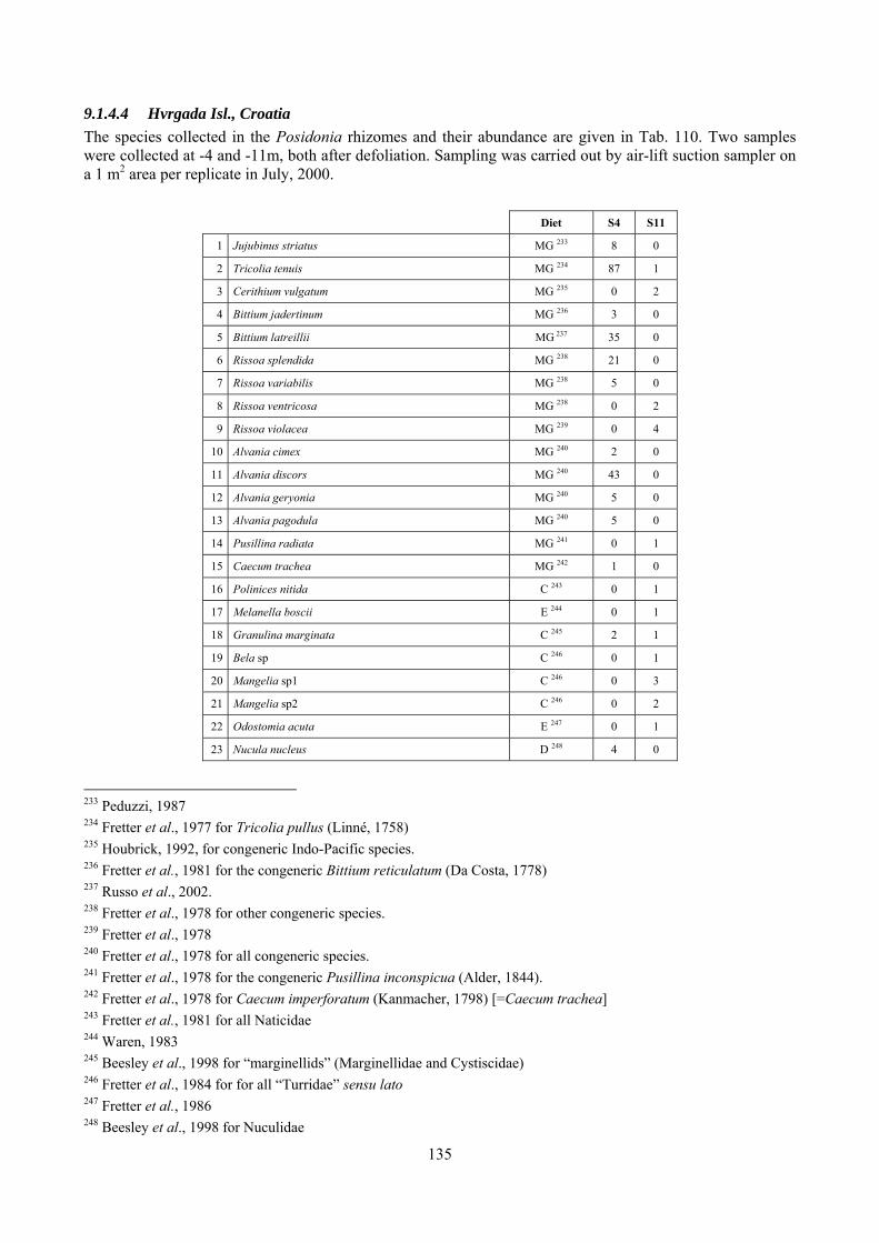
135

9.1.4.4 Hvrgada Isl., Croatia The species collected in the Posidonia rhizomes and their abundance are given in Tab. 110. Two samples were collected at -4 and -11m, both after defoliation. Sampling was carried out by air-lift suction sampler on a 1 m2 area per replicate in July, 2000.

Diet S4 S11

1 Jujubinus striatus MG 233 8 0

2 Tricolia tenuis MG 234 87 1

3 Cerithium vulgatum MG 235 0 2

4 Bittium jadertinum MG 236 3 0

5 Bittium latreillii MG 237 35 0

6 Rissoa splendida MG 238 21 0

7 Rissoa variabilis MG 238 5 0

8 Rissoa ventricosa MG 238 0 2

9 Rissoa violacea MG 239 0 4

10 Alvania cimex MG 240 2 0

11 Alvania discors MG 240 43 0

12 Alvania geryonia MG 240 5 0

13 Alvania pagodula MG 240 5 0

14 Pusillina radiata MG 241 0 1

15 Caecum trachea MG 242 1 0

16 Polinices nitida C 243 0 1

17 Melanella boscii E 244 0 1

18 Granulina marginata C 245 2 1

19 Bela sp C 246 0 1

20 Mangelia sp1 C 246 0 3

21 Mangelia sp2 C 246 0 2

22 Odostomia acuta E 247 0 1

23 Nucula nucleus D 248 4 0

233 Peduzzi, 1987 234 Fretter et al., 1977 for Tricolia pullus (Linné, 1758) 235 Houbrick, 1992, for congeneric Indo-Pacific species. 236 Fretter et al., 1981 for the congeneric Bittium reticulatum (Da Costa, 1778) 237 Russo et al., 2002. 238 Fretter et al., 1978 for other congeneric species. 239 Fretter et al., 1978 240 Fretter et al., 1978 for all congeneric species. 241 Fretter et al., 1978 for the congeneric Pusillina inconspicua (Alder, 1844). 242 Fretter et al., 1978 for Caecum imperforatum (Kanmacher, 1798) [=Caecum trachea] 243 Fretter et al., 1981 for all Naticidae 244 Waren, 1983 245 Beesley et al., 1998 for “marginellids” (Marginellidae and Cystiscidae) 246 Fretter et al., 1984 for for all “Turridae” sensu lato 247 Fretter et al., 1986 248 Beesley et al., 1998 for Nuculidae

136

Diet S4 S11

24 Modiolarca subpicta F 249 2 0

25 Pododesmus patelliformis F 249 0 1

26 Thyasira flexuosa SY 250 7 0

27 Mysella bidentata F 251 2 0

28 Parvicardium exiguum F 252 5 1

29 Venus verrucosa F 253 0 8

30 Gouldia minima F 253 12 2

31 Callista chione F 253 0 1

TOTAL NUMBER OF SPECIMENS 249 33

Tab. 110 – Quali-quantitative data of the Posidonia rhizomes samples, Hvrgada Is., Croatia

The shallow water sample has a much higher abundance of specimens, with a difference of an order of magnitude (249 vs 33). By a population structure point of view (Tab. 105), species richness is almost the same at the two stations but with a low percentage of shared species (12.9%). Shannon diversity index (H’) is lower in shallow water (2.123) than in deep water (2.556) and the same trend is shown by evenness (0.734 in shallow water and 0.902 in deep water). Therefore, the assemblage at the two depths is different both in terms of species composition, faunal abundance and diversity indices.

Replicate S H' J'

S4 18 2.123 0.734

S11 17 2.556 0.902

Tab. 111 – Biodiversity indices values for Posidonia rhizomes samples, Giglio Isl.

Diversity and equitability indices are influenced by dominance phenomena (Tab. 112, Tab. 113). Tricolia tenuis is the dominant species in the shallow water station (34.9%) while Venus verrucosa, a filter feeding venerid clam, is the dominant species in the deeper water station (24.2%). The second dominant species is Alvania discors (17.3%) in shallow water and Rissoa violacea (12.1%) in deep water. These differences further support the hypothesis that the two stations host different species assemblages. Moreover, the deeper water one probably has a greater percentage of sediment since the dominant presence of an infaunal filter feeder.

Diet S4 S11

1 Jujubinus striatus MG 3.2% -

2 Tricolia tenuis MG 34.9% 3.0%

3 Cerithium vulgatum MG - 6.1%

4 Bittium jadertinum MG 1.2% -

5 Bittium latreillii MG 14.1% -

249 Beesley et al., 1998 for Pteriomorphia (Mytiloida, Arcoida, Pterioida, Limoida and Ostreoida) 250 Dias Passos et al., 2007 251 Beesley et al., 1998 for Galeommatoidea 252 Beesley et al., 1998 for the whole family Cardiidae 253 Beesley et al., 1998 for the whole family Veneridae

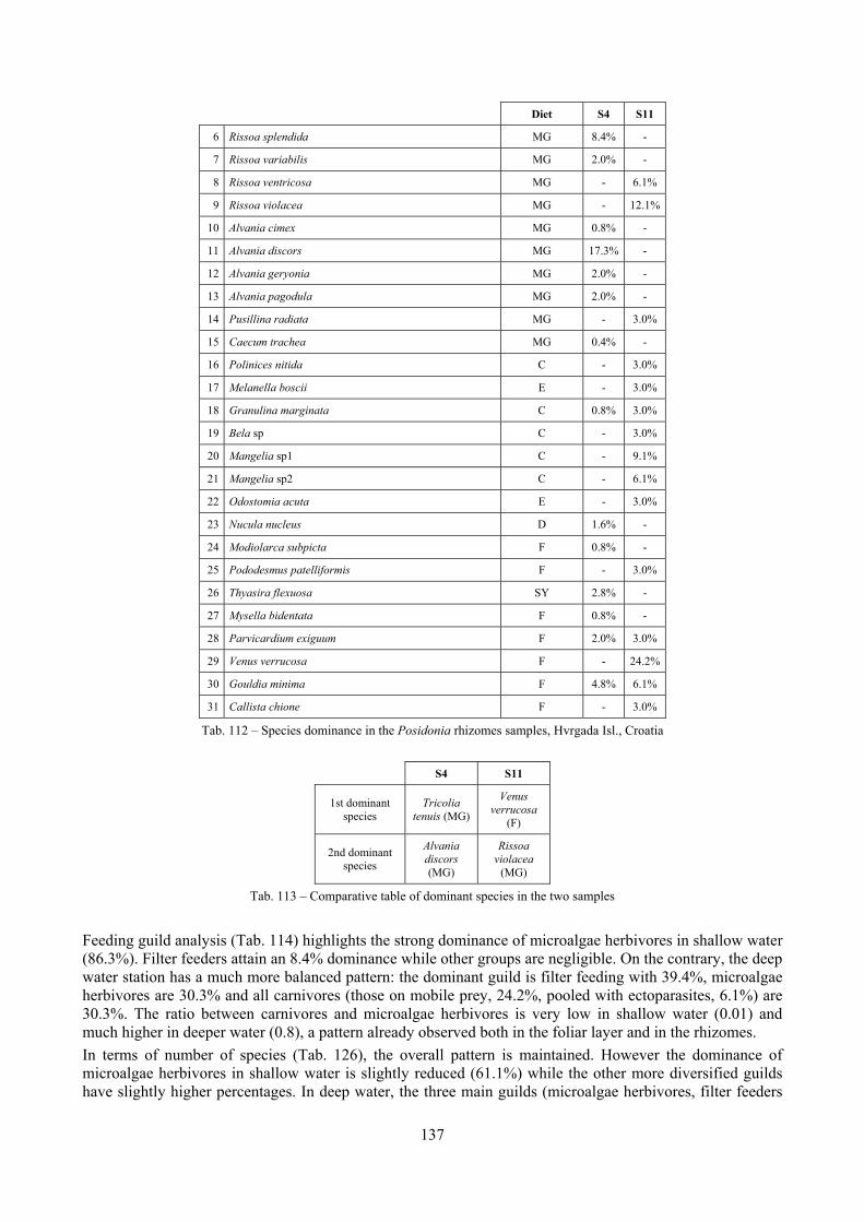
137

Diet S4 S11

6 Rissoa splendida MG 8.4% -

7 Rissoa variabilis MG 2.0% -

8 Rissoa ventricosa MG - 6.1%

9 Rissoa violacea MG - 12.1%

10 Alvania cimex MG 0.8% -

11 Alvania discors MG 17.3% -

12 Alvania geryonia MG 2.0% -

13 Alvania pagodula MG 2.0% -

14 Pusillina radiata MG - 3.0%

15 Caecum trachea MG 0.4% -

16 Polinices nitida C - 3.0%

17 Melanella boscii E - 3.0%

18 Granulina marginata C 0.8% 3.0%

19 Bela sp C - 3.0%

20 Mangelia sp1 C - 9.1%

21 Mangelia sp2 C - 6.1%

22 Odostomia acuta E - 3.0%

23 Nucula nucleus D 1.6% -

24 Modiolarca subpicta F 0.8% -

25 Pododesmus patelliformis F - 3.0%

26 Thyasira flexuosa SY 2.8% -

27 Mysella bidentata F 0.8% -

28 Parvicardium exiguum F 2.0% 3.0%

29 Venus verrucosa F - 24.2%

30 Gouldia minima F 4.8% 6.1%

31 Callista chione F - 3.0%

Tab. 112 – Species dominance in the Posidonia rhizomes samples, Hvrgada Isl., Croatia

S4 S11

1st dominant species

Tricolia tenuis (MG)

Venus verrucosa

(F)

2nd dominant species

Alvania discors (MG)

Rissoa violacea

(MG)

Tab. 113 – Comparative table of dominant species in the two samples

Feeding guild analysis (Tab. 114) highlights the strong dominance of microalgae herbivores in shallow water (86.3%). Filter feeders attain an 8.4% dominance while other groups are negligible. On the contrary, the deep water station has a much more balanced pattern: the dominant guild is filter feeding with 39.4%, microalgae herbivores are 30.3% and all carnivores (those on mobile prey, 24.2%, pooled with ectoparasites, 6.1%) are 30.3%. The ratio between carnivores and microalgae herbivores is very low in shallow water (0.01) and much higher in deeper water (0.8), a pattern already observed both in the foliar layer and in the rhizomes. In terms of number of species (Tab. 126), the overall pattern is maintained. However the dominance of microalgae herbivores in shallow water is slightly reduced (61.1%) while the other more diversified guilds have slightly higher percentages. In deep water, the three main guilds (microalgae herbivores, filter feeders

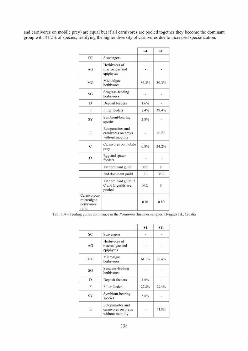
138

and carnivores on mobile prey) are equal but if all carnivores are pooled together they become the dominant group with 41.2% of species, testifying the higher diversity of carnivores due to increased specialization.

S4 S11

SC Scavengers - -

AG Herbivores of macroalgae and epiphytes

- -

MG Microalgae herbivores 86.3% 30.3%

SG Seagrass-feeding herbivores - -

D Deposit feeders 1.6% -

F Filter feeders 8.4% 39.4%

SY Symbiont-bearing species 2.8% -

E Ectoparasites and carnivores on preys without mobility

- 6.1%

C Carnivores on mobile prey 0.8% 24.2%

O Egg and spawn feeders - -

1st dominant guild MG F

2nd dominant guild F MG

1st dominant guild if C and E guilds are pooled

MG F

Carnivorous/ microalgae herbivores ratio

0.01 0.80

Tab. 114 – Feeding guilds dominance in the Posidonia rhizomes samples, Hvrgada Isl., Croatia

S4 S11

SC Scavengers - -

AG Herbivores of macroalgae and epiphytes

- -

MG Microalgae herbivores 61.1% 29.4%

SG Seagrass-feeding herbivores - -

D Deposit feeders 5.6% -

F Filter feeders 22.2% 29.4%

SY Symbiont-bearing species 5.6% -

E Ectoparasites and carnivores on preys without mobility

- 11.8%

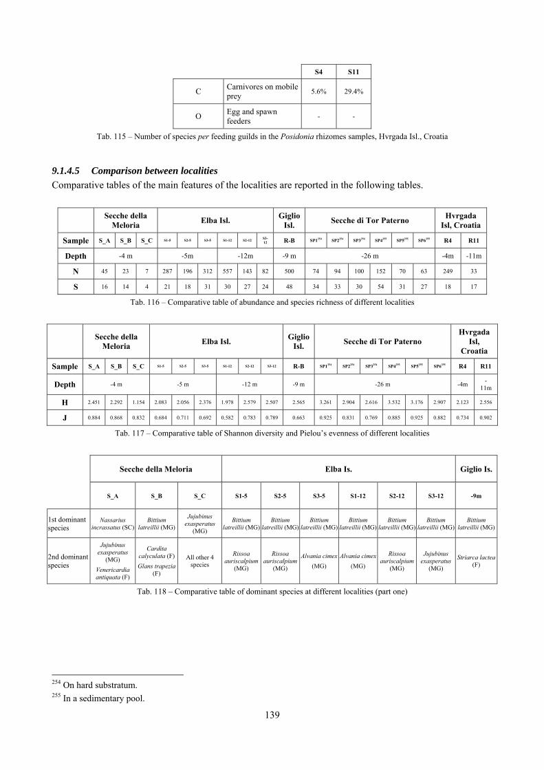
139

S4 S11

C Carnivores on mobile prey 5.6% 29.4%

O Egg and spawn feeders - -

Tab. 115 – Number of species per feeding guilds in the Posidonia rhizomes samples, Hvrgada Isl., Croatia

9.1.4.5 Comparison between localities Comparative tables of the main features of the localities are reported in the following tables.

Secche della Meloria Elba Isl. Giglio

Isl. Secche di Tor Paterno Hvrgada Isl, Croatia

Sample S_A S_B S_C S1-5 S2-5 S3-5 S1-12 S2-12 S3-12 R-B SP1254 SP2254 SP3254 SP4255 SP5255 SP6255 R4 R11

Depth -4 m -5m -12m -9 m -26 m -4m -11m

N 45 23 7 287 196 312 557 143 82 500 74 94 100 152 70 63 249 33

S 16 14 4 21 18 31 30 27 24 48 34 33 30 54 31 27 18 17

Tab. 116 – Comparative table of abundance and species richness of different localities

Secche della Meloria Elba Isl. Giglio

Isl. Secche di Tor Paterno Hvrgada

Isl, Croatia

Sample S_A S_B S_C S1-5 S2-5 S3-5 S1-12 S2-12 S3-12 R-B SP1254 SP2254 SP3254 SP4255 SP5255 SP6255 R4 R11

Depth -4 m -5 m -12 m -9 m -26 m -4m -11m

H 2.451 2.292 1.154 2.083 2.056 2.376 1.978 2.579 2.507 2.565 3.261 2.904 2.616 3.532 3.176 2.907 2.123 2.556

J 0.884 0.868 0.832 0.684 0.711 0.692 0.582 0.783 0.789 0.663 0.925 0.831 0.769 0.885 0.925 0.882 0.734 0.902

Tab. 117 – Comparative table of Shannon diversity and Pielou’s evenness of different localities

Secche della Meloria Elba Is. Giglio Is.

S_A S_B S_C S1-5 S2-5 S3-5 S1-12 S2-12 S3-12 -9m

1st dominant species

Nassarius incrassatus (SC)

Bittium latreillii (MG)

Jujubinus exasperatus

(MG)

Bittium latreillii (MG)

Bittium latreillii (MG)

Bittium latreillii (MG)

Bittium latreillii (MG)

Bittium latreillii (MG)

Bittium latreillii (MG)

Bittium latreillii (MG)

2nd dominant species

Jujubinus exasperatus

(MG) Venericardia antiquata (F)

Cardita calyculata (F) Glans trapezia

(F)

All other 4 species

Rissoa auriscalpium

(MG)

Rissoa auriscalpium

(MG)

Alvania cimex(MG)

Alvania cimex(MG)

Rissoa auriscalpium

(MG)

Jujubinus exasperatus

(MG)

Striarca lactea (F)

Tab. 118 – Comparative table of dominant species at different localities (part one)

254 On hard substratum. 255 In a sedimentary pool.

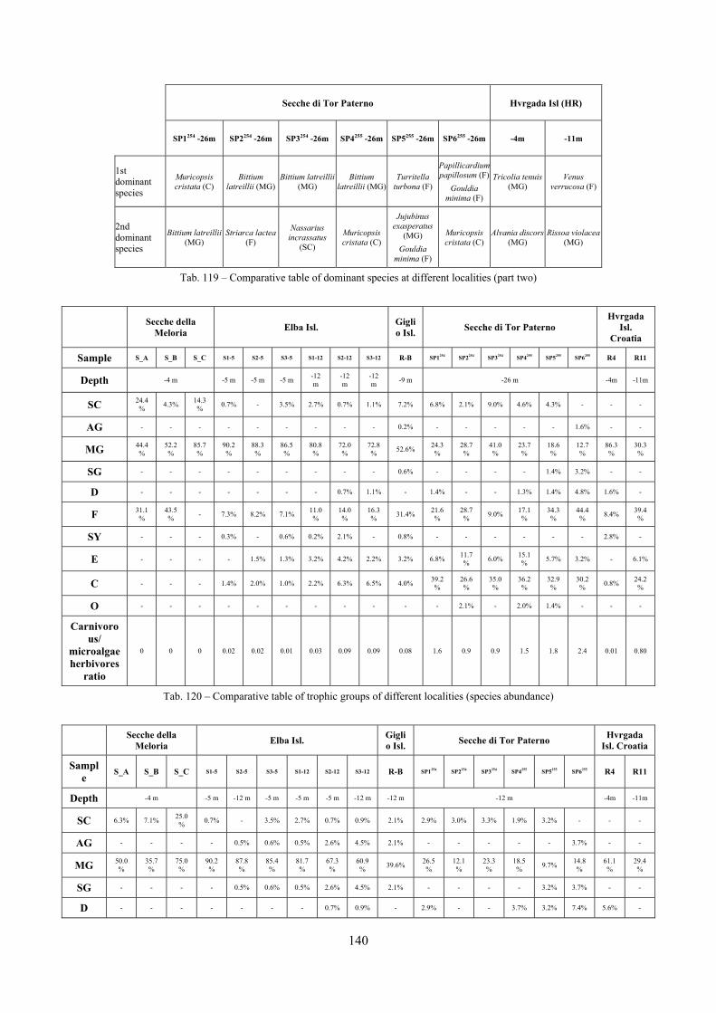
140

Secche di Tor Paterno Hvrgada Isl (HR)

SP1254 -26m SP2254 -26m SP3254 -26m SP4255 -26m SP5255 -26m SP6255 -26m -4m -11m

1st dominant species

Muricopsis cristata (C)

Bittium latreillii (MG)

Bittium latreillii(MG)

Bittium latreillii (MG)

Turritella turbona (F)

Papillicardium papillosum (F)

Gouldia minima (F)

Tricolia tenuis (MG)

Venus verrucosa (F)

2nd dominant species

Bittium latreillii(MG)

Striarca lactea (F)

Nassarius incrassatus

(SC)

Muricopsis cristata (C)

Jujubinus exasperatus

(MG) Gouldia

minima (F)

Muricopsis cristata (C)

Alvania discors (MG)

Rissoa violacea (MG)

Tab. 119 – Comparative table of dominant species at different localities (part two)

Secche della Meloria Elba Isl. Gigli

o Isl. Secche di Tor Paterno Hvrgada

Isl. Croatia

Sample S_A S_B S_C S1-5 S2-5 S3-5 S1-12 S2-12 S3-12 R-B SP1254 SP2254 SP3254 SP4255 SP5255 SP6255 R4 R11

Depth -4 m -5 m -5 m -5 m -12 m

-12 m

-12 m -9 m -26 m -4m -11m

SC 24.4% 4.3% 14.3

% 0.7% - 3.5% 2.7% 0.7% 1.1% 7.2% 6.8% 2.1% 9.0% 4.6% 4.3% - - -

AG - - - - - - - - - 0.2% - - - - - 1.6% - -

MG 44.4%

52.2%

85.7%

90.2%

88.3%

86.5%

80.8%

72.0%

72.8% 52.6% 24.3

% 28.7%

41.0%

23.7%

18.6%

12.7%

86.3%

30.3%

SG - - - - - - - - - 0.6% - - - - 1.4% 3.2% - -

D - - - - - - - 0.7% 1.1% - 1.4% - - 1.3% 1.4% 4.8% 1.6% -

F 31.1%

43.5% - 7.3% 8.2% 7.1% 11.0

% 14.0%

16.3% 31.4% 21.6

% 28.7% 9.0% 17.1

% 34.3%

44.4% 8.4% 39.4

%

SY - - - 0.3% - 0.6% 0.2% 2.1% - 0.8% - - - - - - 2.8% -

E - - - - 1.5% 1.3% 3.2% 4.2% 2.2% 3.2% 6.8% 11.7% 6.0% 15.1

% 5.7% 3.2% - 6.1%

C - - - 1.4% 2.0% 1.0% 2.2% 6.3% 6.5% 4.0% 39.2%

26.6%

35.0%

36.2%

32.9%

30.2% 0.8% 24.2

%

O - - - - - - - - - - - 2.1% - 2.0% 1.4% - - -

Carnivorous/

microalgae herbivores

ratio

0 0 0 0.02 0.02 0.01 0.03 0.09 0.09 0.08 1.6 0.9 0.9 1.5 1.8 2.4 0.01 0.80

Tab. 120 – Comparative table of trophic groups of different localities (species abundance)

Secche della Meloria Elba Isl. Gigli

o Isl. Secche di Tor Paterno Hvrgada Isl. Croatia

Sample S_A S_B S_C S1-5 S2-5 S3-5 S1-12 S2-12 S3-12 R-B SP1254 SP2254 SP3254 SP4255 SP5255 SP6255 R4 R11

Depth -4 m -5 m -12 m -5 m -5 m -5 m -12 m -12 m -12 m -4m -11m

SC 6.3% 7.1% 25.0% 0.7% - 3.5% 2.7% 0.7% 0.9% 2.1% 2.9% 3.0% 3.3% 1.9% 3.2% - - -

AG - - - - 0.5% 0.6% 0.5% 2.6% 4.5% 2.1% - - - - - 3.7% - -

MG 50.0%

35.7%

75.0%

90.2%

87.8%

85.4%

81.7%

67.3%

60.9% 39.6% 26.5

% 12.1%

23.3%

18.5% 9.7% 14.8

% 61.1%

29.4%

SG - - - - 0.5% 0.6% 0.5% 2.6% 4.5% 2.1% - - - - 3.2% 3.7% - -

D - - - - - - - 0.7% 0.9% - 2.9% - - 3.7% 3.2% 7.4% 5.6% -

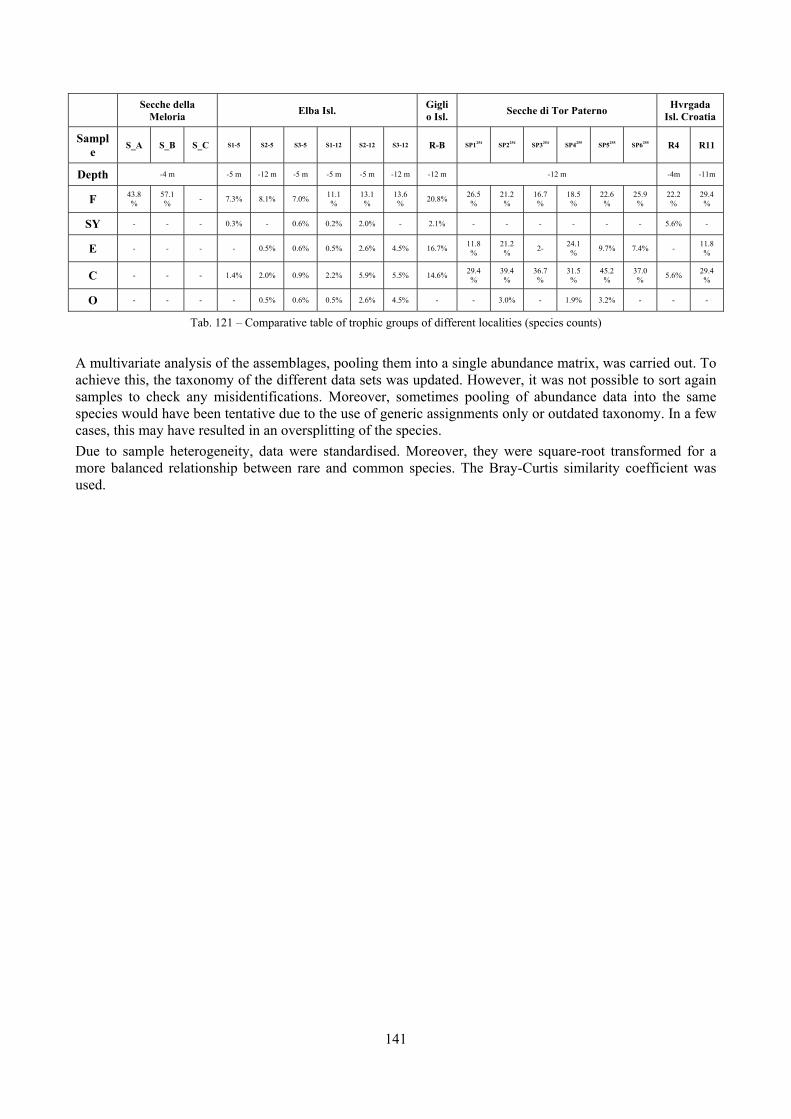
141

Secche della Meloria Elba Isl. Gigli

o Isl. Secche di Tor Paterno Hvrgada Isl. Croatia

Sample S_A S_B S_C S1-5 S2-5 S3-5 S1-12 S2-12 S3-12 R-B SP1254 SP2254 SP3254 SP4255 SP5255 SP6255 R4 R11

Depth -4 m -5 m -12 m -5 m -5 m -5 m -12 m -12 m -12 m -4m -11m

F 43.8%

57.1% - 7.3% 8.1% 7.0% 11.1

% 13.1%

13.6% 20.8% 26.5

% 21.2%

16.7%

18.5%

22.6%

25.9%

22.2%

29.4%

SY - - - 0.3% - 0.6% 0.2% 2.0% - 2.1% - - - - - - 5.6% -

E - - - - 0.5% 0.6% 0.5% 2.6% 4.5% 16.7% 11.8%

21.2% 2- 24.1

% 9.7% 7.4% - 11.8%

C - - - 1.4% 2.0% 0.9% 2.2% 5.9% 5.5% 14.6% 29.4%

39.4%

36.7%

31.5%

45.2%

37.0% 5.6% 29.4

%

O - - - - 0.5% 0.6% 0.5% 2.6% 4.5% - - 3.0% - 1.9% 3.2% - - -

Tab. 121 – Comparative table of trophic groups of different localities (species counts)

A multivariate analysis of the assemblages, pooling them into a single abundance matrix, was carried out. To achieve this, the taxonomy of the different data sets was updated. However, it was not possible to sort again samples to check any misidentifications. Moreover, sometimes pooling of abundance data into the same species would have been tentative due to the use of generic assignments only or outdated taxonomy. In a few cases, this may have resulted in an oversplitting of the species. Due to sample heterogeneity, data were standardised. Moreover, they were square-root transformed for a more balanced relationship between rare and common species. The Bray-Curtis similarity coefficient was used.

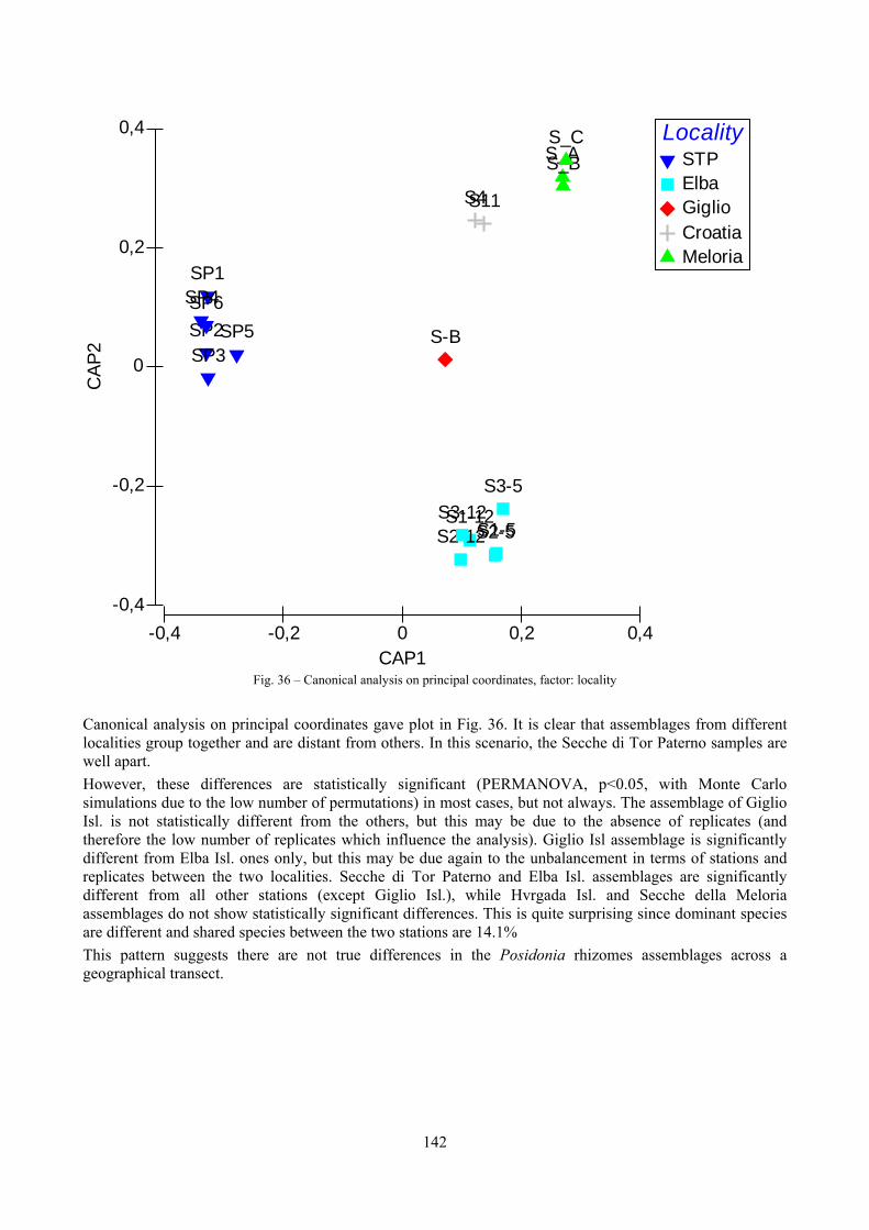
142

Fig. 36 – Canonical analysis on principal coordinates, factor: locality

Canonical analysis on principal coordinates gave plot in Fig. 36. It is clear that assemblages from different localities group together and are distant from others. In this scenario, the Secche di Tor Paterno samples are well apart. However, these differences are statistically significant (PERMANOVA, p<0.05, with Monte Carlo simulations due to the low number of permutations) in most cases, but not always. The assemblage of Giglio Isl. is not statistically different from the others, but this may be due to the absence of replicates (and therefore the low number of replicates which influence the analysis). Giglio Isl assemblage is significantly different from Elba Isl. ones only, but this may be due again to the unbalancement in terms of stations and replicates between the two localities. Secche di Tor Paterno and Elba Isl. assemblages are significantly different from all other stations (except Giglio Isl.), while Hvrgada Isl. and Secche della Meloria assemblages do not show statistically significant differences. This is quite surprising since dominant species are different and shared species between the two stations are 14.1% This pattern suggests there are not true differences in the Posidonia rhizomes assemblages across a geographical transect.

-0,4 -0,2 0 0,2 0,4CAP1

-0,4

-0,2

0

0,2

0,4

CAP

2

LocalitySTPElbaGiglioCroatiaMeloria

SP1

SP2SP3

SP4

SP5SP6

S1-5S2-5

S3-5S1-12

S2-12S3-12

S-B

S4S11

S_AS_BS_C

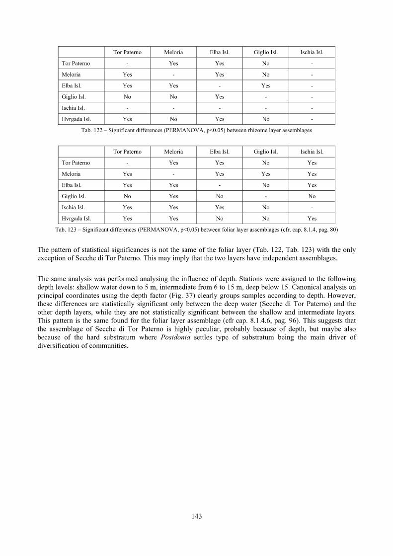
143

Tor Paterno Meloria Elba Isl. Giglio Isl. Ischia Isl.

Tor Paterno - Yes Yes No -

Meloria Yes - Yes No -

Elba Isl. Yes Yes - Yes -

Giglio Isl. No No Yes - -

Ischia Isl. - - - - -

Hvrgada Isl. Yes No Yes No -

Tab. 122 – Significant differences (PERMANOVA, p<0.05) between rhizome layer assemblages

Tor Paterno Meloria Elba Isl. Giglio Isl. Ischia Isl.

Tor Paterno - Yes Yes No Yes

Meloria Yes - Yes Yes Yes

Elba Isl. Yes Yes - No Yes

Giglio Isl. No Yes No - No

Ischia Isl. Yes Yes Yes No -

Hvrgada Isl. Yes Yes No No Yes

Tab. 123 – Significant differences (PERMANOVA, p<0.05) between foliar layer assemblages (cfr. cap. 8.1.4, pag. 80)

The pattern of statistical significances is not the same of the foliar layer (Tab. 122, Tab. 123) with the only exception of Secche di Tor Paterno. This may imply that the two layers have independent assemblages. The same analysis was performed analysing the influence of depth. Stations were assigned to the following depth levels: shallow water down to 5 m, intermediate from 6 to 15 m, deep below 15. Canonical analysis on principal coordinates using the depth factor (Fig. 37) clearly groups samples according to depth. However, these differences are statistically significant only between the deep water (Secche di Tor Paterno) and the other depth layers, while they are not statistically significant between the shallow and intermediate layers. This pattern is the same found for the foliar layer assemblage (cfr cap. 8.1.4.6, pag. 96). This suggests that the assemblage of Secche di Tor Paterno is highly peculiar, probably because of depth, but maybe also because of the hard substratum where Posidonia settles type of substratum being the main driver of diversification of communities.

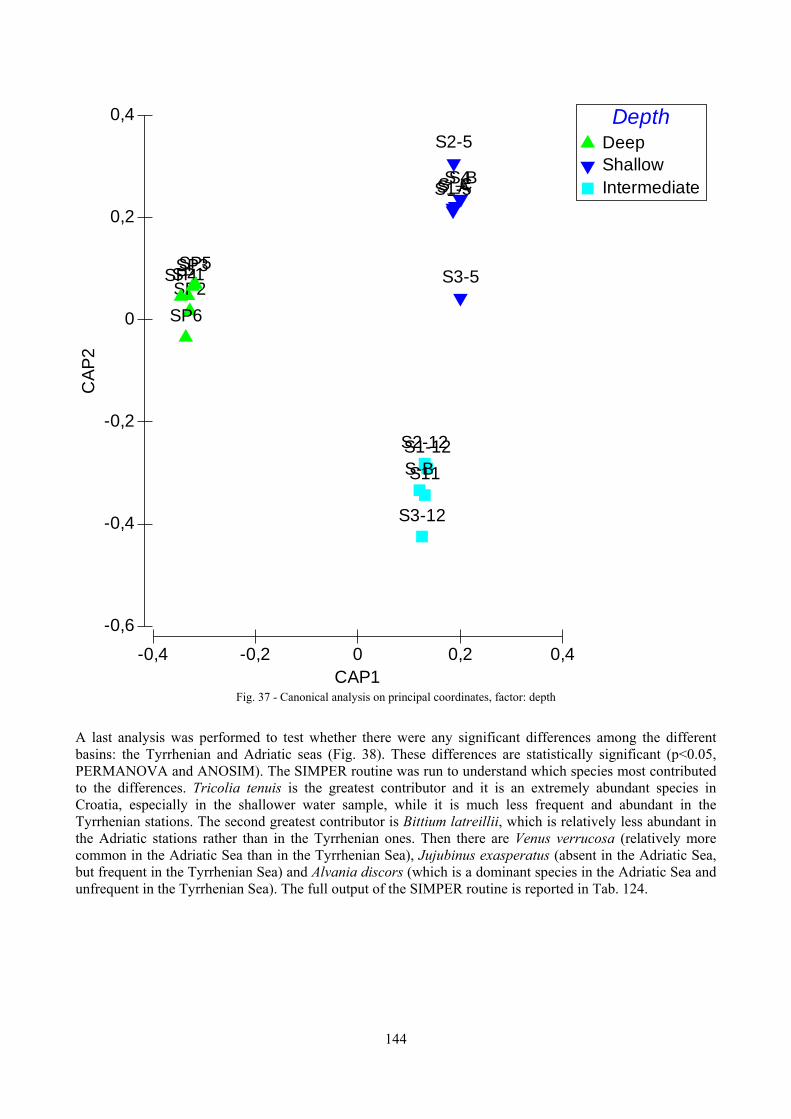
144

Fig. 37 - Canonical analysis on principal coordinates, factor: depth

A last analysis was performed to test whether there were any significant differences among the different basins: the Tyrrhenian and Adriatic seas (Fig. 38). These differences are statistically significant (p<0.05, PERMANOVA and ANOSIM). The SIMPER routine was run to understand which species most contributed to the differences. Tricolia tenuis is the greatest contributor and it is an extremely abundant species in Croatia, especially in the shallower water sample, while it is much less frequent and abundant in the Tyrrhenian stations. The second greatest contributor is Bittium latreillii, which is relatively less abundant in the Adriatic stations rather than in the Tyrrhenian ones. Then there are Venus verrucosa (relatively more common in the Adriatic Sea than in the Tyrrhenian Sea), Jujubinus exasperatus (absent in the Adriatic Sea, but frequent in the Tyrrhenian Sea) and Alvania discors (which is a dominant species in the Adriatic Sea and unfrequent in the Tyrrhenian Sea). The full output of the SIMPER routine is reported in Tab. 124.

-0,4 -0,2 0 0,2 0,4CAP1

-0,6

-0,4

-0,2

0

0,2

0,4C

AP2

DepthDeepShallowIntermediate

SP1SP2SP3SP4SP5

SP6

S1-5

S2-5

S3-5

S4S_AS_BS_C

S1-12S2-12

S3-12

S-BS11

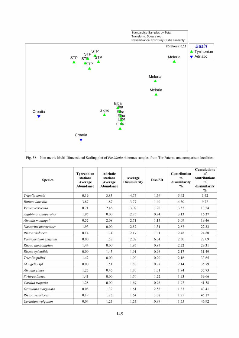
145

Fig. 38 – Non metric Multi-Dimensional Scaling plot of Posidonia rhizomes samples from Tor Paterno and comparison localities

Species

Tyrrenhian stations Average

Abundance

Adriatic stations Average

Abundance

Average Dissimilarity Diss/SD

Contribution to

dissimilarity %

Cumulations of

contributions to

dissimilarity%

Tricolia tenuis 0.19 3.83 4.75 1.56 5.42 5.42

Bittium latreillii 3.87 1.87 3.77 1.40 4.30 9.72

Venus verrucosa 0.71 2.46 3.09 1.20 3.52 13.24

Jujubinus exasperatus 1.95 0.00 2.75 0.84 3.13 16.37

Alvania montagui 0.52 2.08 2.71 1.15 3.09 19.46

Nassarius incrassatus 1.93 0.00 2.52 1.31 2.87 22.32

Rissoa violacea 0.14 1.74 2.17 1.01 2.48 24.80

Parvicardium exiguum 0.00 1.58 2.02 6.04 2.30 27.09

Rissoa auriscalpium 1.44 0.00 1.95 0.87 2.22 29.31

Rissoa splendida 0.00 1.45 1.91 0.96 2.17 31.49

Tricolia pullus 1.42 0.00 1.90 0.90 2.16 33.65

Mangelia sp1 0.00 1.51 1.88 0.97 2.14 35.79

Alvania cimex 1.23 0.45 1.70 1.01 1.94 37.73

Striarca lactea 1.41 0.00 1.70 1.22 1.93 39.66

Cardita trapezia 1.28 0.00 1.69 0.96 1.92 41.58

Granulina marginata 0.08 1.32 1.61 2.58 1.83 43.41

Rissoa ventricosa 0.19 1.23 1.54 1.08 1.75 45.17

Cerithium vulgatum 0.04 1.23 1.53 0.99 1.75 46.92

Standardise Samples by TotalTransform: Square rootResemblance: S17 Bray Curtis similarity

BasinTyrrhenianAdriatic

STP

STPSTP

STPSTPSTP

ElbaElba

ElbaElba

ElbaElba

Giglio

Croatia

Croatia

Meloria

Meloria

Meloria

2D Stress: 0,11

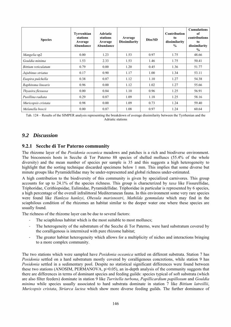
146

Species

Tyrrenhian stations Average

Abundance

Adriatic stations Average

Abundance

Average Dissimilarity Diss/SD

Contribution to

dissimilarity %

Cumulations of

contributions to

dissimilarity%

Mangelia sp2 0.00 1.23 1.53 0.97 1.75 48.66

Gouldia minima 1.53 2.33 1.53 1.46 1.75 50.41

Bittium reticulatum 0.79 0.00 1.20 0.45 1.36 51.77

Jujubinus striatus 0.17 0.90 1.17 1.00 1.34 53.11

Euspira pulchella 0.38 0.87 1.12 1.10 1.27 54.38

Raphitoma linearis 0.96 0.00 1.12 1.02 1.27 55.66

Thyasira flexuosa 0.00 0.84 1.10 0.96 1.25 56.91

Pusillina radiata 0.29 0.87 1.09 1.18 1.25 58.16

Muricopsis cristata 0.98 0.00 1.09 0.73 1.24 59.40

Melanella boscii 0.00 0.87 1.08 0.97 1.24 60.64

Tab. 124 – Results of the SIMPER analysis representing the breakdown of average dissimilarity between the Tyrrhenian and the Adriatic stations

9.2 Discussion

9.2.1 Secche di Tor Paterno community The rhizome layer of the Posidonia oceanica meadows and patches is a rich and biodiverse environment. The biocoenosis hosts in Secche di Tor Paterno 88 species of shelled molluscs (55.4% of the whole diversity) and the mean number of species per sample is 35 and this suggests a high heterogeneity to highlight that the sorting technique discarded specimens below 1 mm. This implies that some diverse but minute groups like Pyramidellidae may be under-represented and global richness under-estimated. A high contribution to the biodiversity of this community is given by specialized carnivores. This group accounts for up to 24.1% of the species richness. This group is characterized by taxa like Fissurellidae, Triphoridae, Cerithiopsidae, Eulimidae, Pyramidellidae. Triphoridae in particular is represented by 6 species, a high percentage of the overall infralittoral Mediterranean fauna. In this environment some very rare species were found like Hanleya hanleyi, Obesula marisnostri, Mathilda gemmulata which may find in the sciaphilous condition of the rhizomes an habitat similar to the deeper water one where these species are usually found. The richness of the rhizome layer can be due to several factors:

‐ The sciaphilous habitat which is the most suitable to most molluscs; ‐ The heterogeneity of the substratum of the Secche di Tor Paterno, were hard substratum covered by

the coralligenous is intermixed with pure rhizome habitat; ‐ The greater habitat heterogeneity which allows for a multiplicity of niches and interactions bringing

to a more complex community. The two stations which were sampled have Posidonia oceanica settled on different substrata. Station 7 has Posidonia settled on a hard substratum mostly covered by coralligenous concretions, while station 9 has Posidonia settled in a sedimentary pool. Despite no statistical significant differences were found between these two stations (ANOSIM, PERMANOVA, p>0.05), an in-depth analysis of the community suggests that there are differences in terms of dominant species and feeding guilds: species typical of soft substrata (which are also filter feeders) dominate in station 9 like Turritella turbona, Papillicardium papillosum and Gouldia minima while species usually associated to hard substrata dominate in station 7 like Bittium latreillii, Muricopsis cristata, Striarca lactea which show more diverse feeding guilds. The further dominance of

147

species of soft substratum affinity may also justify the outsiding of replicate SP6 in the cluster diagram (Fig. 32) and MDS plot (Fig. 33). The richness of carnivores is sustained by a rich diversity of other species. For example, polychaetes represent a good share of the community and are the probable food of Turridae which are here represented by 10 species (11% of the whole rhizomes diversity). Comparison with the characteristic species cited in literature (Harmelin, 1964 for the mattes; Pérès & Picard, 1964 for the coralligenous) shows little consistency. Only Venus verrucosa is present as typical species of the mattes and Lima lima as characteristic of the coralligenous.

9.2.2 Comparison with other data sets The diversity of species can achieve remarkable numbers in the rhizomes with peaks of 54 species per sample in Secche di Tor Paterno. This is a special case however, since the Posidonia patches lay in a coralligenous substratum which certainly help enriching the rhizomes community due to the presence of ecoclines. Most other samples have a species abundance between 15 and 30 species per sample. Shannon diversity is at its highest in Secche di Tor Paterno where values are all above 2.6 and 50% of samples have it above 3. Again this is probably the result of an ecoclinal gradient towards the coralligenous. In any case, most other samples have Shannon index above 2. The foliar layer had significantly lower values (pag. 101) and a much lower equitability due to more significant cases of species dominance. The dominant species in the rhizome layer is often Bittium latreillii: 11 samples on 18, 61.1%. The other samples show a great heterogeneity of dominant species, since every sample has a different one. The presence of dominants doesn’t seem to be correlated with depth. Considering the feeding guilds, dominant species are often microalgae herbivores, but also scavengers (Nassarius incrassatus in Secche della Meloria), carnivores on mobile prey (Muricopsis cristata in Secche di Tor Paterno) and filter feeders (Turritella turbona, Papillicardium papillosum and Gouldia minima in Secche di Tor Paterno, Venus verrucosa in Hrvgada Isl.). Moreover, microalgae herbivores are present in all samples, filter-feeders in all but one (94.4%), carnivores on mobile prey in 15 samples (83.3%), ectoparasites in 13 (72.2%), scavengers in 14 (77.8%). The other feeding guilds are present less frequently. Remarkable that despite the rhizome layer is suitable for infaunal bivalves a very low frequence and abundance of detritus feeders is present. Quantitatively, the rhizome layer hosts a higher number of specimens than the foliar layer. However, the ability to sample this abundance is strictly dependand on the sampling technique. If the leaves are removed the effectiveness of sampling in the rhizomes is much higher and all localities where defoliation was carried out show a higher number of specimes in the rhizomes than in the leaves (Secche di Tor Paterno, Giglio Isl, Hrvgada Isl.). Secche della Meloria samples are particularly poor (7 to 45 specimens, 4 to 16 species) which is an anomaly in the context of very shallow stations, however, the very small sampling area (0.25 × 0.25 m) has certainly played a role. The carnivorous/microalgae herbivores ratio increases with depth and shows a pattern similar to the foliar layer. This ratio is usually below 0.1 above -15 m while it grows to 2.4 at -25 m. This is probably the result of lower light irradiance. Remarkably, the station in Croatia at -11 m has a 0.8 ratio which is in the order of magnitude of deeper stations of the Tyrrhenian Sea. As already observed for the foliar layer, the rhizome layer in Croatia shows the presence of deeper water characters in shallower levels, and this may be due to reduced water transparency or other environmental factors which would deserve further study.

148

10 Analysis of the coralligenous species assemblage The coralligenous biocoenosis (C, Pérès & Picard, 1964) is a typical biocoenosis of hard substrata and is characterized by two conditions:

1. The availability of hard substrata, either rocky or concretionary; 2. The sciaphilous environment and algal dominance.

Two characteristic mollusc species are cited by Pérès & Picard (1964): Chlamys pes-felis [Manupecten pesfelis (Linné, 1758)] and Lima squamosa [Lima lima (Linné, 1758)]. The coralligenous habitat is a hard substratum of biogenic origin that is mainly produced by the accumulation of calcareous encrusting algae growing in dim light conditions (Ballesteros, 2006). One of the main characters of this environment is therefore to be sciaphilic. The bioherm of coralline algae is a very complex three-dimensional structure which host living algae in the illuminated upper part of the concretions, suspension feeders in the lower part of the concretions, wall cavities and overhangs, borers inside the concretions and soft-substratum fauna in the sediment deposited in cavities and holes. Therefore, coralligenous habitat has a high microspatial heterogeneity making difficult a quantitative sampling approach. Moreover, each niche can have great variation in environmental factors (e.g. light, water movement and sedimentation rates) adding to the great heterogeneity of the assemblage. Coralligenous extends from -15/20 m to the deeper circalittoral (120 m circa). In Secche di Tor Paterno samples come from shallow water compared to the bathymetric tolerance of the habitat since samples come from -20/27 m. Fifteen facies are described for this biocoenosis (Giaccone et al., 2009). Three are encountered in the Secche di Tor Paterno:

‐ association with Eunicella singularis (Esper, 1791), on horizontal and sub-horizontal substrata; ‐ association with Eunicella cavolinii (Koch, 1887) on the walls and underside of boulders; ‐ association with Paramuricea clavata (Risso, 1826) on the reef drop-offs below 30 m.

This habitat exists in the Mediterranean Sea only and it is of conservation concern due to its biodiversity and the heavy anthropogenic pressures the Mediterranean coastal environments experience. The habitat is considered within the 1170 “Reefs” habitat of the Directive 92/43/CE “Habitat” and therefore sites with this habitat can be considered for inclusion in the Natura 2000 network (European Commission – DG Environment, 2007). Moreover, it is considered important for conservation by the Protocol Concerning Specially Protected Areas and Biological Diversity in the Mediterranean of the Barcelona Convention. Moreover, this habitat is reported to be the second most important hot spot of species diversity in the Mediterranean Sea after the Posidonia oceanica meadows (Boudouresque, 2004) which have enjoyed much more research. Most of the published literature on this habitat is from the north-western Mediterranean: Banyuls-sur-Mer (Laubier, 1966), Marseille (Hong, 1980), Islas Medas (Gili & Ros, 1984). Some further work has been carried out on the very peculiar North Adriatic coralligenous outcrops called “tegnue” (see Casellato & Stefanon, 2008 for a review). The Tyrrhenian Sea coralligenous assemblages were not studied much. Virgilio et al. (2006) analyzed the spatial and temporal variations of epibenthic assemblages at Calafuria, south of Livorno, but biodiversity reports lack. The molluscan assemblages in particular were studied in the Mediterranean France locations (Laubier, 1966; Hong, 1980; Huelin & Ros, 1984), in Mediterranean Spain (Martin et al., 1990, Salas & Hergueta, 1986) but no similar works are available for infralittoral coralligenous reefs in the Tyrrhenian Sea. Sampling of the coralligenous biocoenosis in Secche di Tor Paterno was carried out in September 1992 by Università La Sapienza (1993) by scraping of 20 × 20 cm area in 5 stations between 21 and 37 meters deep. Forty species (2 were nudibranchs) and 449 specimens (2 nudibranchs) were recorded alive.

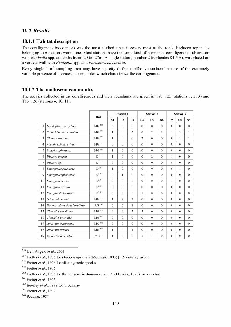
149

10.1 Results

10.1.1 Habitat description The coralligenous biocoenosis was the most studied since it covers most of the reefs. Eighteen replicates belonging to 6 stations were done. Most stations have the same kind of horizontal coralligenous substratum with Eunicella spp. at depths from -20 to -27m. A single station, number 2 (replicates S4-5-6), was placed on a vertical wall with Eunicella spp. and Paramuricea clavata. Every single 1 m2 sampling area may have a pretty different effective surface because of the extremely variable presence of crevices, stones, holes which characterize the coralligenous.

10.1.2 The molluscan community The species collected in the coralligenous and their abundance are given in Tab. 125 (stations 1, 2, 3) and Tab. 126 (stations 4, 10, 11).

Diet Station 1 Station 2 Station 3

S1 S2 S3 S4 S5 S6 S7 S8 S9

1 Lepidopleurus cajetanus MG 256 0 0 0 0 0 0 0 0 0

2 Callochiton septemvalvis MG 256 1 0 3 0 2 1 1 3 1

3 Chiton corallinus MG 256 1 0 0 2 0 0 3 1 1

4 Acanthochitona crinita MG 256 0 0 0 0 0 0 0 0 0

5 Polyplacophora sp. MG 256 1 0 0 0 0 0 0 0 0

6 Diodora graeca E 257 1 0 0 0 2 0 1 0 0

7 Diodora sp. E 257 0 0 0 0 0 0 3 0 0

8 Emarginula octaviana E 258 1 0 0 0 0 0 0 1 0

9 Emarginula punctulum E 258 0 1 0 0 0 0 0 0 0

10 Emarginula rosea E 259 0 0 0 0 0 0 1 0 0

11 Emarginula sicula E 258 0 0 0 0 0 0 0 0 0

12 Emarginella huzardii E 258 0 0 0 1 0 0 0 0 0

13 Scissurella costata MG 260 1 2 3 0 0 0 0 0 0

14 Haliotis tuberculata lamellosa AG 261 0 0 1 0 0 0 0 0 0

15 Clanculus corallinus MG 262 0 0 2 2 0 0 0 0 0

16 Clanculus cruciatus MG 262 0 0 0 0 0 0 0 0 0

17 Jujubinus exasperatus MG 263 0 0 0 0 0 0 0 0 0

18 Jujubinus striatus MG 264 1 0 1 0 0 0 0 0 0

19 Calliostoma conulum MG 14 1 0 0 1 1 0 0 0 0

256 Dell’Angelo et al., 2001 257 Fretter et al., 1976 for Diodora apertura (Montagu, 1803) [= Diodora graeca] 258 Fretter et al., 1976 for all congeneric species 259 Fretter et al., 1976 260 Fretter et al., 1976 for the congeneric Anatoma crispata (Fleming, 1828) [Scissurella] 261 Fretter et al., 1976 262 Beesley et al., 1998 for Trochinae 263 Fretter et al., 1977 264 Peduzzi, 1987

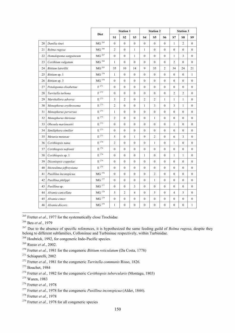
150

Diet Station 1 Station 2 Station 3

S1 S2 S3 S4 S5 S6 S7 S8 S9

20 Danilia tinei MG 265 0 0 0 0 0 0 1 2 0

21 Bolma rugosa MG 266 2 0 1 1 0 0 0 0 0

22 Homalopoma sanguineum MG 267 0 0 1 0 0 0 1 3 0

23 Cerithium vulgatum MG 268 1 0 0 0 0 0 2 0 0

24 Bittium latreillii MG 269 35 10 14 9 35 2 34 24 21

25 Bittium sp. 1 MG 270 1 0 0 0 0 0 0 0 1

26 Bittium sp. 3 MG 270 0 0 0 0 0 0 0 0 0

27 Petalopoma elisabettae F 271 0 0 0 0 0 0 0 0 0

28 Turritella turbona F 272 0 0 0 0 0 0 2 2 0

29 Marshallora adversa E 273 3 2 0 2 2 1 1 1 0

30 Monophorus erythrosoma E 273 2 0 0 1 3 0 3 1 0

31 Monophorus perversus E 273 1 0 0 0 0 0 0 0 0

32 Monophorus thiriotae E 273 2 0 0 0 1 0 0 0 0

33 Obesula marisnostri E 273 0 0 0 0 0 0 1 0 0

34 Similiphora similior E 273 0 0 0 0 0 0 0 0 0

35 Metaxia metaxae E 273 5 0 1 9 2 0 6 3 0

36 Cerithiopsis nana E 274 2 0 0 0 1 0 1 0 0

37 Cerithiopsis nofronii E 274 0 0 0 0 0 0 0 0 0

38 Cerithiopsis sp. 1 E 274 0 0 0 1 0 0 1 1 0

39 Dizoniopsis coppolae E 274 0 0 0 0 0 0 0 0 0

40 Sticteulima jeffreysiana E 275 0 0 0 0 0 0 0 0 0

41 Pusillina inconspicua MG 276 0 0 0 0 2 0 0 0 0

42 Pusillina philippi MG 277 0 0 0 0 1 0 0 0 0

43 Pusillina sp. MG 277 0 0 3 0 0 0 0 0 0

44 Alvania cancellata MG 278 5 2 4 0 5 0 4 5 0

45 Alvania cimex MG 279 0 0 0 0 0 0 0 0 0

46 Alvania discors MG 279 1 0 0 0 0 0 0 0 1

265 Fretter et al., 1977 for the systematically close Trochidae 266 Beu et al., 1979 267 Due to the absence of specific references, it is hypothesized the same feeding guild of Bolma rugosa, despite they belong to different subfamilies, Colloniinae and Turbininae respectively, within Turbinidae. 268 Houbrick, 1992, for congeneric Indo-Pacific species. 269 Russo et al., 2002. 270 Fretter et al., 1981 for the congeneric Bittium reticulatum (Da Costa, 1778) 271 Schiaparelli, 2002 272 Fretter et al., 1981 for the congeneric Turritella communis Risso, 1826. 273 Bouchet, 1984 274 Fretter et al., 1982 for the congeneric Cerithiopsis tubercularis (Montagu, 1803) 275 Waren, 1983 276 Fretter et al., 1978 277 Fretter et al., 1978 for the congeneric Pusillina inconspicua (Alder, 1844). 278 Fretter et al., 1978 279 Fretter et al., 1978 for all congeneric species

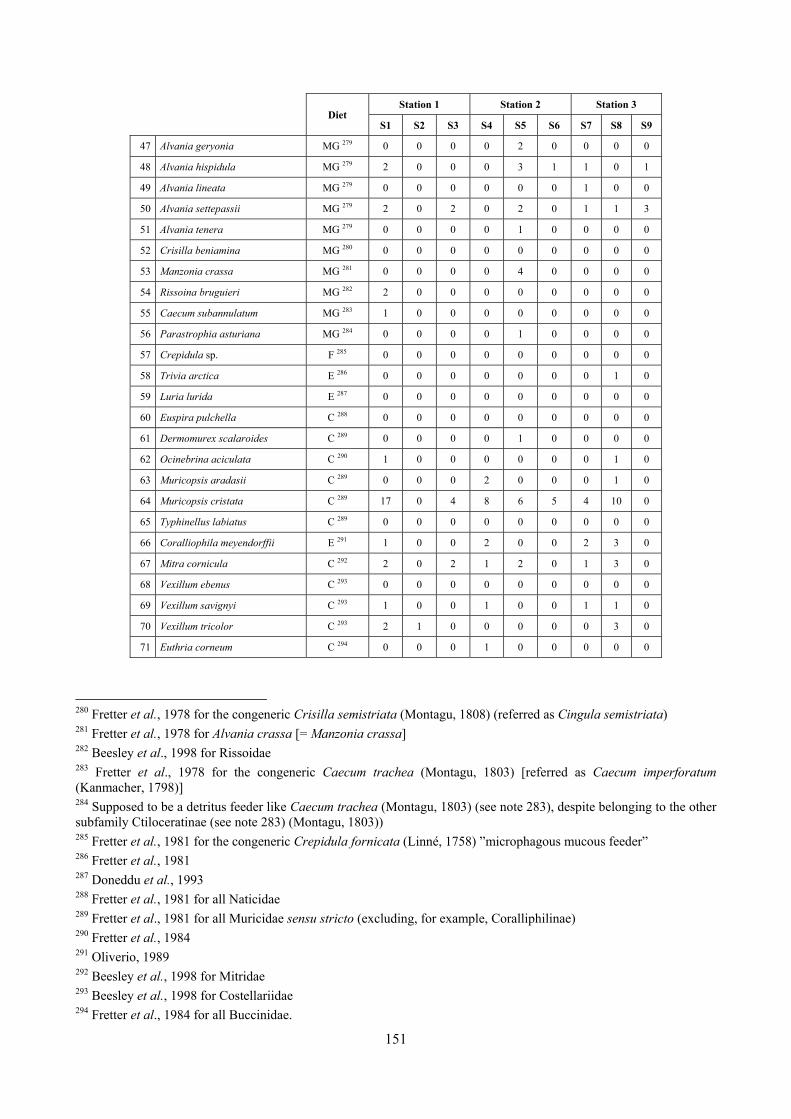
151

Diet Station 1 Station 2 Station 3

S1 S2 S3 S4 S5 S6 S7 S8 S9

47 Alvania geryonia MG 279 0 0 0 0 2 0 0 0 0

48 Alvania hispidula MG 279 2 0 0 0 3 1 1 0 1

49 Alvania lineata MG 279 0 0 0 0 0 0 1 0 0

50 Alvania settepassii MG 279 2 0 2 0 2 0 1 1 3

51 Alvania tenera MG 279 0 0 0 0 1 0 0 0 0

52 Crisilla beniamina MG 280 0 0 0 0 0 0 0 0 0

53 Manzonia crassa MG 281 0 0 0 0 4 0 0 0 0

54 Rissoina bruguieri MG 282 2 0 0 0 0 0 0 0 0

55 Caecum subannulatum MG 283 1 0 0 0 0 0 0 0 0

56 Parastrophia asturiana MG 284 0 0 0 0 1 0 0 0 0

57 Crepidula sp. F 285 0 0 0 0 0 0 0 0 0

58 Trivia arctica E 286 0 0 0 0 0 0 0 1 0

59 Luria lurida E 287 0 0 0 0 0 0 0 0 0

60 Euspira pulchella C 288 0 0 0 0 0 0 0 0 0

61 Dermomurex scalaroides C 289 0 0 0 0 1 0 0 0 0

62 Ocinebrina aciculata C 290 1 0 0 0 0 0 0 1 0

63 Muricopsis aradasii C 289 0 0 0 2 0 0 0 1 0

64 Muricopsis cristata C 289 17 0 4 8 6 5 4 10 0

65 Typhinellus labiatus C 289 0 0 0 0 0 0 0 0 0

66 Coralliophila meyendorffii E 291 1 0 0 2 0 0 2 3 0

67 Mitra cornicula C 292 2 0 2 1 2 0 1 3 0

68 Vexillum ebenus C 293 0 0 0 0 0 0 0 0 0

69 Vexillum savignyi C 293 1 0 0 1 0 0 1 1 0

70 Vexillum tricolor C 293 2 1 0 0 0 0 0 3 0

71 Euthria corneum C 294 0 0 0 1 0 0 0 0 0

280 Fretter et al., 1978 for the congeneric Crisilla semistriata (Montagu, 1808) (referred as Cingula semistriata) 281 Fretter et al., 1978 for Alvania crassa [= Manzonia crassa] 282 Beesley et al., 1998 for Rissoidae 283 Fretter et al., 1978 for the congeneric Caecum trachea (Montagu, 1803) [referred as Caecum imperforatum (Kanmacher, 1798)] 284 Supposed to be a detritus feeder like Caecum trachea (Montagu, 1803) (see note 283), despite belonging to the other subfamily Ctiloceratinae (see note 283) (Montagu, 1803)) 285 Fretter et al., 1981 for the congeneric Crepidula fornicata (Linné, 1758) ”microphagous mucous feeder” 286 Fretter et al., 1981 287 Doneddu et al., 1993 288 Fretter et al., 1981 for all Naticidae 289 Fretter et al., 1981 for all Muricidae sensu stricto (excluding, for example, Coralliphilinae) 290 Fretter et al., 1984 291 Oliverio, 1989 292 Beesley et al., 1998 for Mitridae 293 Beesley et al., 1998 for Costellariidae 294 Fretter et al., 1984 for all Buccinidae.

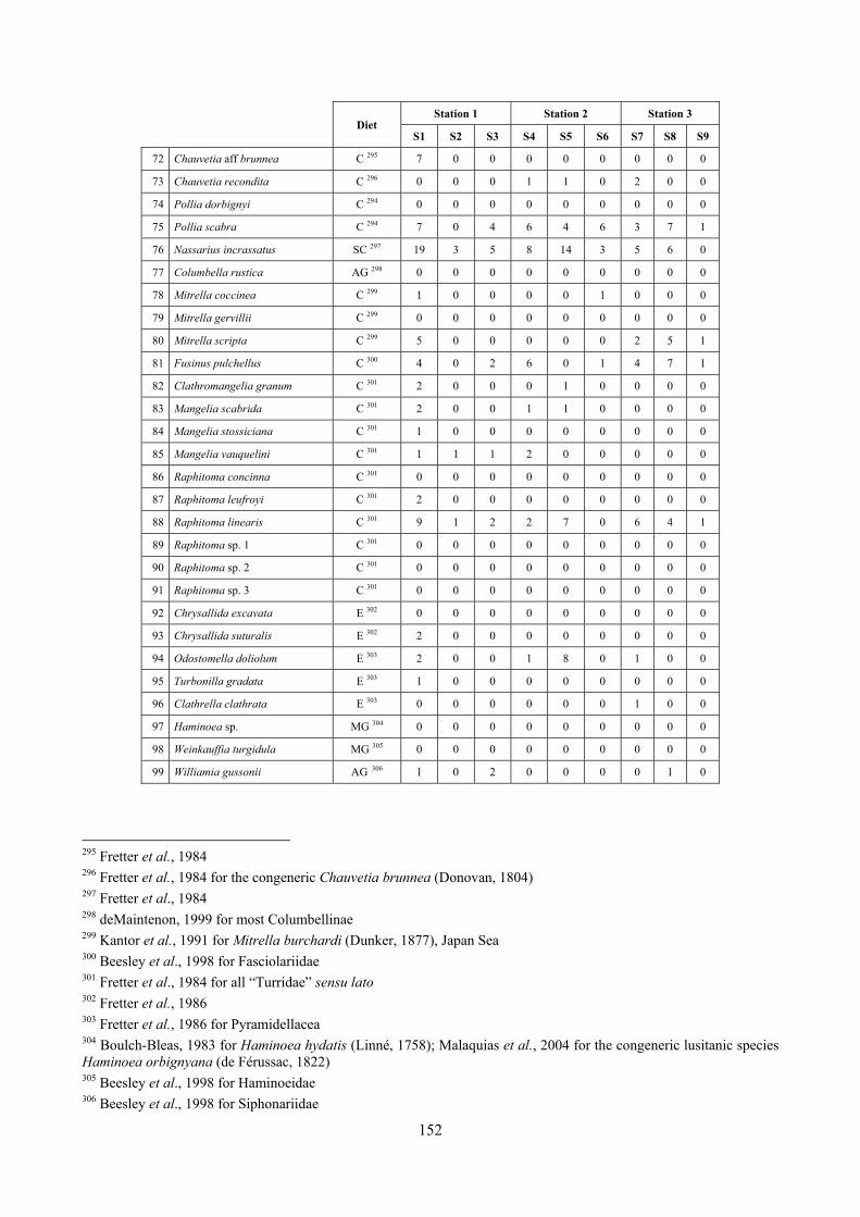
152

Diet Station 1 Station 2 Station 3

S1 S2 S3 S4 S5 S6 S7 S8 S9

72 Chauvetia aff brunnea C 295 7 0 0 0 0 0 0 0 0

73 Chauvetia recondita C 296 0 0 0 1 1 0 2 0 0

74 Pollia dorbignyi C 294 0 0 0 0 0 0 0 0 0

75 Pollia scabra C 294 7 0 4 6 4 6 3 7 1

76 Nassarius incrassatus SC 297 19 3 5 8 14 3 5 6 0

77 Columbella rustica AG 298 0 0 0 0 0 0 0 0 0

78 Mitrella coccinea C 299 1 0 0 0 0 1 0 0 0

79 Mitrella gervillii C 299 0 0 0 0 0 0 0 0 0

80 Mitrella scripta C 299 5 0 0 0 0 0 2 5 1

81 Fusinus pulchellus C 300 4 0 2 6 0 1 4 7 1

82 Clathromangelia granum C 301 2 0 0 0 1 0 0 0 0

83 Mangelia scabrida C 301 2 0 0 1 1 0 0 0 0

84 Mangelia stossiciana C 301 1 0 0 0 0 0 0 0 0

85 Mangelia vauquelini C 301 1 1 1 2 0 0 0 0 0

86 Raphitoma concinna C 301 0 0 0 0 0 0 0 0 0

87 Raphitoma leufroyi C 301 2 0 0 0 0 0 0 0 0

88 Raphitoma linearis C 301 9 1 2 2 7 0 6 4 1

89 Raphitoma sp. 1 C 301 0 0 0 0 0 0 0 0 0

90 Raphitoma sp. 2 C 301 0 0 0 0 0 0 0 0 0

91 Raphitoma sp. 3 C 301 0 0 0 0 0 0 0 0 0

92 Chrysallida excavata E 302 0 0 0 0 0 0 0 0 0

93 Chrysallida suturalis E 302 2 0 0 0 0 0 0 0 0

94 Odostomella doliolum E 303 2 0 0 1 8 0 1 0 0

95 Turbonilla gradata E 303 1 0 0 0 0 0 0 0 0

96 Clathrella clathrata E 303 0 0 0 0 0 0 1 0 0

97 Haminoea sp. MG 304 0 0 0 0 0 0 0 0 0

98 Weinkauffia turgidula MG 305 0 0 0 0 0 0 0 0 0

99 Williamia gussonii AG 306 1 0 2 0 0 0 0 1 0

295 Fretter et al., 1984 296 Fretter et al., 1984 for the congeneric Chauvetia brunnea (Donovan, 1804) 297 Fretter et al., 1984 298 deMaintenon, 1999 for most Columbellinae 299 Kantor et al., 1991 for Mitrella burchardi (Dunker, 1877), Japan Sea 300 Beesley et al., 1998 for Fasciolariidae 301 Fretter et al., 1984 for all “Turridae” sensu lato 302 Fretter et al., 1986 303 Fretter et al., 1986 for Pyramidellacea 304 Boulch-Bleas, 1983 for Haminoea hydatis (Linné, 1758); Malaquias et al., 2004 for the congeneric lusitanic species Haminoea orbignyana (de Férussac, 1822) 305 Beesley et al., 1998 for Haminoeidae 306 Beesley et al., 1998 for Siphonariidae

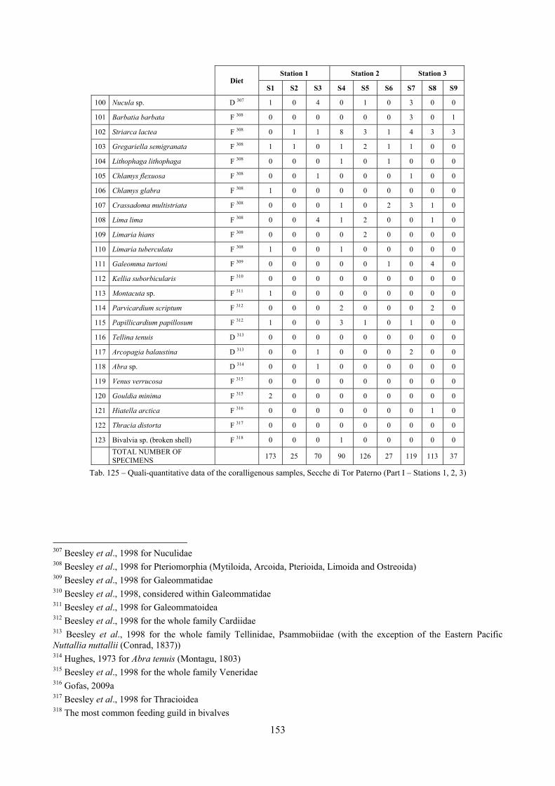
153

Diet Station 1 Station 2 Station 3

S1 S2 S3 S4 S5 S6 S7 S8 S9

100 Nucula sp. D 307 1 0 4 0 1 0 3 0 0

101 Barbatia barbata F 308 0 0 0 0 0 0 3 0 1

102 Striarca lactea F 308 0 1 1 8 3 1 4 3 3

103 Gregariella semigranata F 308 1 1 0 1 2 1 1 0 0

104 Lithophaga lithophaga F 308 0 0 0 1 0 1 0 0 0

105 Chlamys flexuosa F 308 0 0 1 0 0 0 1 0 0

106 Chlamys glabra F 308 1 0 0 0 0 0 0 0 0

107 Crassadoma multistriata F 308 0 0 0 1 0 2 3 1 0

108 Lima lima F 308 0 0 4 1 2 0 0 1 0

109 Limaria hians F 308 0 0 0 0 2 0 0 0 0

110 Limaria tuberculata F 308 1 0 0 1 0 0 0 0 0

111 Galeomma turtoni F 309 0 0 0 0 0 1 0 4 0

112 Kellia suborbicularis F 310 0 0 0 0 0 0 0 0 0

113 Montacuta sp. F 311 1 0 0 0 0 0 0 0 0

114 Parvicardium scriptum F 312 0 0 0 2 0 0 0 2 0

115 Papillicardium papillosum F 312 1 0 0 3 1 0 1 0 0

116 Tellina tenuis D 313 0 0 0 0 0 0 0 0 0

117 Arcopagia balaustina D 313 0 0 1 0 0 0 2 0 0

118 Abra sp. D 314 0 0 1 0 0 0 0 0 0

119 Venus verrucosa F 315 0 0 0 0 0 0 0 0 0

120 Gouldia minima F 315 2 0 0 0 0 0 0 0 0

121 Hiatella arctica F 316 0 0 0 0 0 0 0 1 0

122 Thracia distorta F 317 0 0 0 0 0 0 0 0 0

123 Bivalvia sp. (broken shell) F 318 0 0 0 1 0 0 0 0 0

TOTAL NUMBER OF SPECIMENS 173 25 70 90 126 27 119 113 37

Tab. 125 – Quali-quantitative data of the coralligenous samples, Secche di Tor Paterno (Part I – Stations 1, 2, 3)

307 Beesley et al., 1998 for Nuculidae 308 Beesley et al., 1998 for Pteriomorphia (Mytiloida, Arcoida, Pterioida, Limoida and Ostreoida) 309 Beesley et al., 1998 for Galeommatidae 310 Beesley et al., 1998, considered within Galeommatidae 311 Beesley et al., 1998 for Galeommatoidea 312 Beesley et al., 1998 for the whole family Cardiidae 313 Beesley et al., 1998 for the whole family Tellinidae, Psammobiidae (with the exception of the Eastern Pacific Nuttallia nuttallii (Conrad, 1837)) 314 Hughes, 1973 for Abra tenuis (Montagu, 1803) 315 Beesley et al., 1998 for the whole family Veneridae 316 Gofas, 2009a 317 Beesley et al., 1998 for Thracioidea 318 The most common feeding guild in bivalves

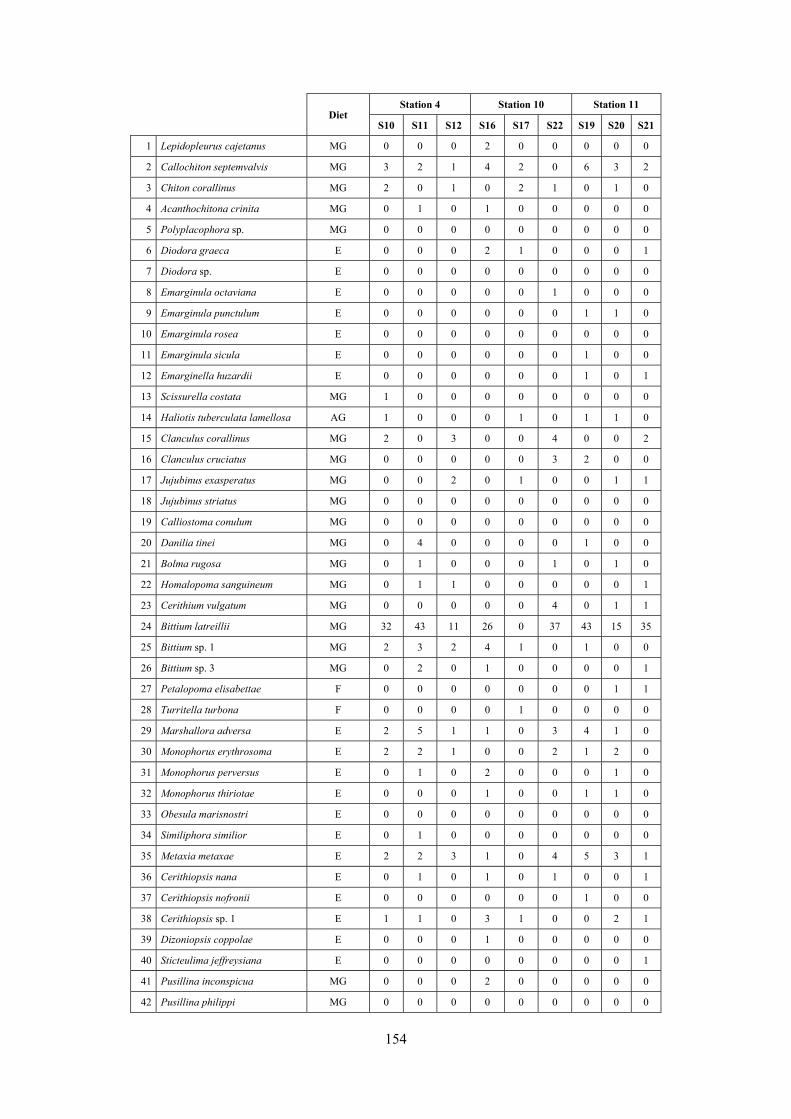
154

Diet Station 4 Station 10 Station 11

S10 S11 S12 S16 S17 S22 S19 S20 S21

1 Lepidopleurus cajetanus MG 0 0 0 2 0 0 0 0 0

2 Callochiton septemvalvis MG 3 2 1 4 2 0 6 3 2

3 Chiton corallinus MG 2 0 1 0 2 1 0 1 0

4 Acanthochitona crinita MG 0 1 0 1 0 0 0 0 0

5 Polyplacophora sp. MG 0 0 0 0 0 0 0 0 0

6 Diodora graeca E 0 0 0 2 1 0 0 0 1

7 Diodora sp. E 0 0 0 0 0 0 0 0 0

8 Emarginula octaviana E 0 0 0 0 0 1 0 0 0

9 Emarginula punctulum E 0 0 0 0 0 0 1 1 0

10 Emarginula rosea E 0 0 0 0 0 0 0 0 0

11 Emarginula sicula E 0 0 0 0 0 0 1 0 0

12 Emarginella huzardii E 0 0 0 0 0 0 1 0 1

13 Scissurella costata MG 1 0 0 0 0 0 0 0 0

14 Haliotis tuberculata lamellosa AG 1 0 0 0 1 0 1 1 0

15 Clanculus corallinus MG 2 0 3 0 0 4 0 0 2

16 Clanculus cruciatus MG 0 0 0 0 0 3 2 0 0

17 Jujubinus exasperatus MG 0 0 2 0 1 0 0 1 1

18 Jujubinus striatus MG 0 0 0 0 0 0 0 0 0

19 Calliostoma conulum MG 0 0 0 0 0 0 0 0 0

20 Danilia tinei MG 0 4 0 0 0 0 1 0 0

21 Bolma rugosa MG 0 1 0 0 0 1 0 1 0

22 Homalopoma sanguineum MG 0 1 1 0 0 0 0 0 1

23 Cerithium vulgatum MG 0 0 0 0 0 4 0 1 1

24 Bittium latreillii MG 32 43 11 26 0 37 43 15 35

25 Bittium sp. 1 MG 2 3 2 4 1 0 1 0 0

26 Bittium sp. 3 MG 0 2 0 1 0 0 0 0 1

27 Petalopoma elisabettae F 0 0 0 0 0 0 0 1 1

28 Turritella turbona F 0 0 0 0 1 0 0 0 0

29 Marshallora adversa E 2 5 1 1 0 3 4 1 0

30 Monophorus erythrosoma E 2 2 1 0 0 2 1 2 0

31 Monophorus perversus E 0 1 0 2 0 0 0 1 0

32 Monophorus thiriotae E 0 0 0 1 0 0 1 1 0

33 Obesula marisnostri E 0 0 0 0 0 0 0 0 0

34 Similiphora similior E 0 1 0 0 0 0 0 0 0

35 Metaxia metaxae E 2 2 3 1 0 4 5 3 1

36 Cerithiopsis nana E 0 1 0 1 0 1 0 0 1

37 Cerithiopsis nofronii E 0 0 0 0 0 0 1 0 0

38 Cerithiopsis sp. 1 E 1 1 0 3 1 0 0 2 1

39 Dizoniopsis coppolae E 0 0 0 1 0 0 0 0 0

40 Sticteulima jeffreysiana E 0 0 0 0 0 0 0 0 1

41 Pusillina inconspicua MG 0 0 0 2 0 0 0 0 0

42 Pusillina philippi MG 0 0 0 0 0 0 0 0 0

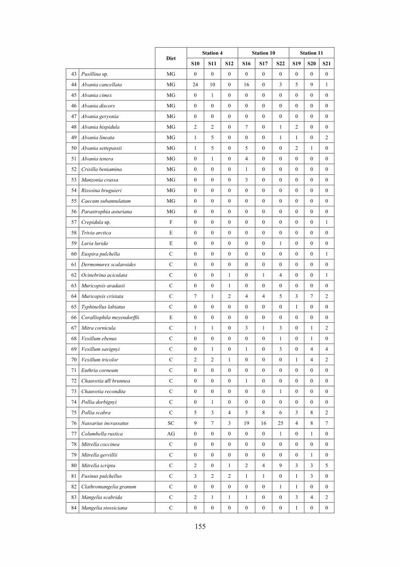
155

Diet Station 4 Station 10 Station 11

S10 S11 S12 S16 S17 S22 S19 S20 S21

43 Pusillina sp. MG 0 0 0 0 0 0 0 0 0

44 Alvania cancellata MG 24 10 0 16 0 3 5 9 1

45 Alvania cimex MG 0 1 0 0 0 0 0 0 0

46 Alvania discors MG 0 0 0 0 0 0 0 0 0

47 Alvania geryonia MG 0 0 0 0 0 0 0 0 0

48 Alvania hispidula MG 2 2 0 7 0 1 2 0 0

49 Alvania lineata MG 1 5 0 0 0 1 1 0 2

50 Alvania settepassii MG 1 5 0 5 0 0 2 1 0

51 Alvania tenera MG 0 1 0 4 0 0 0 0 0

52 Crisilla beniamina MG 0 0 0 1 0 0 0 0 0

53 Manzonia crassa MG 0 0 0 3 0 0 0 0 0

54 Rissoina bruguieri MG 0 0 0 0 0 0 0 0 0

55 Caecum subannulatum MG 0 0 0 0 0 0 0 0 0

56 Parastrophia asturiana MG 0 0 0 0 0 0 0 0 0

57 Crepidula sp. F 0 0 0 0 0 0 0 0 1

58 Trivia arctica E 0 0 0 0 0 0 0 0 0

59 Luria lurida E 0 0 0 0 0 1 0 0 0

60 Euspira pulchella C 0 0 0 0 0 0 0 0 1

61 Dermomurex scalaroides C 0 0 0 0 0 0 0 0 0

62 Ocinebrina aciculata C 0 0 1 0 1 4 0 0 1

63 Muricopsis aradasii C 0 0 1 0 0 0 0 0 0

64 Muricopsis cristata C 7 1 2 4 4 5 3 7 2

65 Typhinellus labiatus C 0 0 0 0 0 0 1 0 0

66 Coralliophila meyendorffii E 0 0 0 0 0 0 0 0 0

67 Mitra cornicula C 1 1 0 3 1 3 0 1 2

68 Vexillum ebenus C 0 0 0 0 0 1 0 1 0

69 Vexillum savignyi C 0 1 0 1 0 3 0 4 4

70 Vexillum tricolor C 2 2 1 0 0 0 1 4 2

71 Euthria corneum C 0 0 0 0 0 0 0 0 0

72 Chauvetia aff brunnea C 0 0 0 1 0 0 0 0 0

73 Chauvetia recondita C 0 0 0 0 0 1 0 0 0

74 Pollia dorbignyi C 0 1 0 0 0 0 0 0 0

75 Pollia scabra C 5 3 4 5 8 6 3 8 2

76 Nassarius incrassatus SC 9 7 3 19 16 25 4 8 7

77 Columbella rustica AG 0 0 0 0 0 1 0 1 0

78 Mitrella coccinea C 0 0 0 0 0 0 0 0 0

79 Mitrella gervillii C 0 0 0 0 0 0 0 1 0

80 Mitrella scripta C 2 0 1 2 4 9 3 3 5

81 Fusinus pulchellus C 3 2 2 1 1 0 1 3 0

82 Clathromangelia granum C 0 0 0 0 0 1 1 0 0

83 Mangelia scabrida C 2 1 1 1 0 0 3 4 2

84 Mangelia stossiciana C 0 0 0 0 0 0 1 0 0

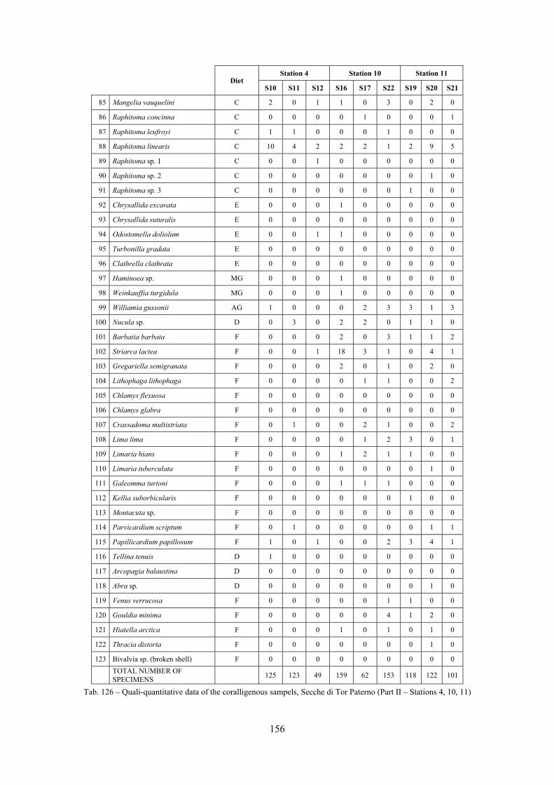
156

Diet Station 4 Station 10 Station 11

S10 S11 S12 S16 S17 S22 S19 S20 S21

85 Mangelia vauquelini C 2 0 1 1 0 3 0 2 0

86 Raphitoma concinna C 0 0 0 0 1 0 0 0 1

87 Raphitoma leufroyi C 1 1 0 0 0 1 0 0 0

88 Raphitoma linearis C 10 4 2 2 2 1 2 9 5

89 Raphitoma sp. 1 C 0 0 1 0 0 0 0 0 0

90 Raphitoma sp. 2 C 0 0 0 0 0 0 0 1 0

91 Raphitoma sp. 3 C 0 0 0 0 0 0 1 0 0

92 Chrysallida excavata E 0 0 0 1 0 0 0 0 0

93 Chrysallida suturalis E 0 0 0 0 0 0 0 0 0

94 Odostomella doliolum E 0 0 1 1 0 0 0 0 0

95 Turbonilla gradata E 0 0 0 0 0 0 0 0 0

96 Clathrella clathrata E 0 0 0 0 0 0 0 0 0

97 Haminoea sp. MG 0 0 0 1 0 0 0 0 0

98 Weinkauffia turgidula MG 0 0 0 1 0 0 0 0 0

99 Williamia gussonii AG 1 0 0 0 2 3 3 1 3

100 Nucula sp. D 0 3 0 2 2 0 1 1 0

101 Barbatia barbata F 0 0 0 2 0 3 1 1 2

102 Striarca lactea F 0 0 1 18 3 1 0 4 1

103 Gregariella semigranata F 0 0 0 2 0 1 0 2 0

104 Lithophaga lithophaga F 0 0 0 0 1 1 0 0 2

105 Chlamys flexuosa F 0 0 0 0 0 0 0 0 0

106 Chlamys glabra F 0 0 0 0 0 0 0 0 0

107 Crassadoma multistriata F 0 1 0 0 2 1 0 0 2

108 Lima lima F 0 0 0 0 1 2 3 0 1

109 Limaria hians F 0 0 0 1 2 1 1 0 0

110 Limaria tuberculata F 0 0 0 0 0 0 0 1 0

111 Galeomma turtoni F 0 0 0 1 1 1 0 0 0

112 Kellia suborbicularis F 0 0 0 0 0 0 1 0 0

113 Montacuta sp. F 0 0 0 0 0 0 0 0 0

114 Parvicardium scriptum F 0 1 0 0 0 0 0 1 1

115 Papillicardium papillosum F 1 0 1 0 0 2 3 4 1

116 Tellina tenuis D 1 0 0 0 0 0 0 0 0

117 Arcopagia balaustina D 0 0 0 0 0 0 0 0 0

118 Abra sp. D 0 0 0 0 0 0 0 1 0

119 Venus verrucosa F 0 0 0 0 0 1 1 0 0

120 Gouldia minima F 0 0 0 0 0 4 1 2 0

121 Hiatella arctica F 0 0 0 1 0 1 0 1 0

122 Thracia distorta F 0 0 0 0 0 0 0 1 0

123 Bivalvia sp. (broken shell) F 0 0 0 0 0 0 0 0 0

TOTAL NUMBER OF SPECIMENS 125 123 49 159 62 153 118 122 101

Tab. 126 – Quali-quantitative data of the coralligenous sampels, Secche di Tor Paterno (Part II – Stations 4, 10, 11)

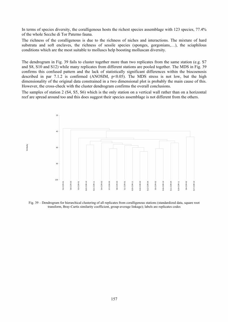
157

In terms of species diversity, the coralligenous hosts the richest species assemblage with 123 species, 77.4% of the whole Secche di Tor Paterno fauna. The richness of the coralligenous is due to the richness of niches and interactions. The mixture of hard substrata and soft enclaves, the richness of sessile species (sponges, gorgonians,…), the sciaphilous conditions which are the most suitable to molluscs help boosting molluscan diversity. The dendrogram in Fig. 39 fails to cluster together more than two replicates from the same station (e.g. S7 and S8, S10 and S12) while many replicates from different stations are pooled together. The MDS in Fig. 39 confirms this confused pattern and the lack of statistically significant differences within the biocoenosis described in par 7.1.2 is confirmed (ANOSIM, p<0.05). The MDS stress is not low, but the high dimensionality of the original data constrained in a two dimensional plot is probably the main cause of this. However, the cross-check with the cluster dendrogram confirms the overall conclusions. The samples of station 2 (S4, S5, S6) which is the only station on a vertical wall rather than on a horizontal reef are spread around too and this does suggest their species assemblage is not different from the others.

Fig. 39 – Dendrogram for hierarchical clustering of all replicates from coralligenous stations (standardized data, square root

transform, Bray-Curtis similarity coefficient, group-average linkage); labels are replicates codes

S2-

CO

R-0

1

S9-

CO

R-0

3

S3-

CO

R-0

1

S22

-CO

R-1

0

S21

-CO

R-1

1

S4-

CO

R-0

2

S7-

CO

R-0

3

S8-

CO

R-0

3

S1-

CO

R-0

1

S20

-CO

R-1

1

S10

-CO

R-0

4

S12

-CO

R-0

4

S5-

CO

R-0

2

S16

-CO

R-1

0

S11

-CO

R-0

4

S19

-CO

R-1

1

S6-

CO

R-0

2

S17

-CO

R-1

0

100

80

60

40

20

Sim

ilarit

y

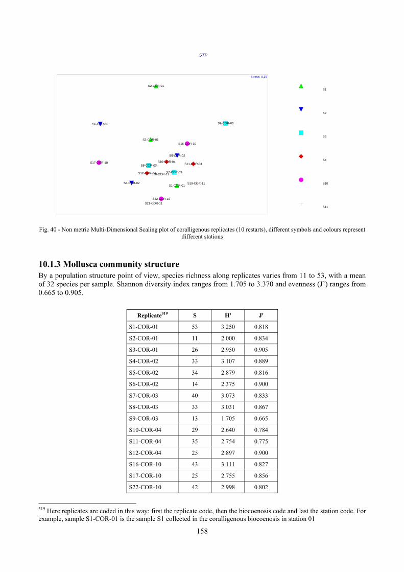
158

Fig. 40 - Non metric Multi-Dimensional Scaling plot of coralligenous replicates (10 restarts), different symbols and colours represent

different stations

10.1.3 Mollusca community structure By a population structure point of view, species richness along replicates varies from 11 to 53, with a mean of 32 species per sample. Shannon diversity index ranges from 1.705 to 3.370 and evenness (J’) ranges from 0.665 to 0.905.

Replicate319 S H' J'

S1-COR-01 53 3.250 0.818

S2-COR-01 11 2.000 0.834

S3-COR-01 26 2.950 0.905

S4-COR-02 33 3.107 0.889

S5-COR-02 34 2.879 0.816

S6-COR-02 14 2.375 0.900

S7-COR-03 40 3.073 0.833

S8-COR-03 33 3.031 0.867

S9-COR-03 13 1.705 0.665

S10-COR-04 29 2.640 0.784

S11-COR-04 35 2.754 0.775

S12-COR-04 25 2.897 0.900

S16-COR-10 43 3.111 0.827

S17-COR-10 25 2.755 0.856

S22-COR-10 42 2.998 0.802

319 Here replicates are coded in this way: first the replicate code, then the biocoenosis code and last the station code. For example, sample S1-COR-01 is the sample S1 collected in the coralligenous biocoenosis in station 01

STP

S1

S2

S3

S4

S10

S11

S1-COR-01

S2-COR-01

S3-COR-01

S4-COR-02

S5-COR-02

S6-COR-02

S7-COR-03

S8-COR-03

S9-COR-03

S10-COR-04S11-COR-04

S12-COR-04

S16-COR-10

S17-COR-10

S22-COR-10

S19-COR-11

S20-COR-11

S21-COR-11

Stress: 0,19

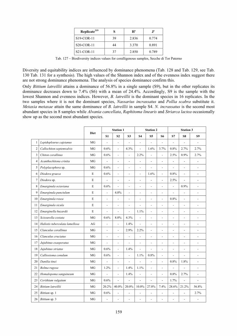
159

Replicate319 S H' J'

S19-COR-11 39 2.836 0.774

S20-COR-11 44 3.370 0.891

S21-COR-11 37 2.850 0.789

Tab. 127 – Biodiversity indices values for coralligenous samples, Secche di Tor Paterno

Diversity and equitability indices are influenced by dominance phenomena (Tab. 128 and Tab. 129, see Tab. 130 Tab. 131 for a synthesis). The high values of the Shannon index and of the evenness index suggest there are not strong dominance phenomena. The analysis of species dominance confirm this. Only Bittium latreillii attains a dominance of 56.8% in a single sample (S9), but in the other replicates its dominance decreases down to 7.4% (S6) with a mean of 24.4%. Accordingly, S9 is the sample with the lowest Shannon and evenness indices. However, B. latreillii is the dominant species in 16 replicates. In the two samples where it is not the dominant species, Nassarius incrassatus and Pollia scabra substitute it. Metaxia metaxae attain the same dominance of B. latreillii in sample S4. N. incrassatus is the second most abundant species in 8 samples while Alvania cancellata, Raphitoma linearis and Striarca lactea occasionally show up as the second most abundant species.

Diet Station 1 Station 2 Station 3

S1 S2 S3 S4 S5 S6 S7 S8 S9

1 Lepidopleurus cajetanus MG - - - - - - - - - 2 Callochiton septemvalvis MG 0.6% - 4.3% - 1.6% 3.7% 0.8% 2.7% 2.7% 3 Chiton corallinus MG 0.6% - - 2.2% - - 2.5% 0.9% 2.7% 4 Acanthochitona crinita MG - - - - - - - - -

5 Polyplacophora sp. MG 0.6% - - - - - - - -

6 Diodora graeca E 0.6% - - - 1.6% - 0.8% - -

7 Diodora sp. E - - - - - - 2.5% - -

8 Emarginula octaviana E 0.6% - - - - - - 0.9% -

9 Emarginula punctulum E - 4.0% - - - - - - -

10 Emarginula rosea E - - - - - - 0.8% - -

11 Emarginula sicula E - - - - - - - - -

12 Emarginella huzardii E - - - 1.1% - - - - -

13 Scissurella costata MG 0.6% 8.0% 4.3% - - - - - -

14 Haliotis tuberculata lamellosa AG - - 1.4% - - - - - -

15 Clanculus corallinus MG - - 2.9% 2.2% - - - - -

16 Clanculus cruciatus MG - - - - - - - - -

17 Jujubinus exasperatus MG - - - - - - - - -

18 Jujubinus striatus MG 0.6% - 1.4% - - - - - -

19 Calliostoma conulum MG 0.6% - - 1.1% 0.8% - - - -

20 Danilia tinei MG - - - - - - 0.8% 1.8% -

21 Bolma rugosa MG 1.2% - 1.4% 1.1% - - - - -

22 Homalopoma sanguineum MG - - 1.4% - - - 0.8% 2.7% -

23 Cerithium vulgatum MG 0.6% - - - - - 1.7% - -

24 Bittium latreillii MG 20.2% 40.0% 20.0% 10.0% 27.8% 7.4% 28.6% 21.2% 56.8%

25 Bittium sp. 1 MG 0.6% - - - - - - - 2.7% 26 Bittium sp. 3 MG - - - - - - - - -

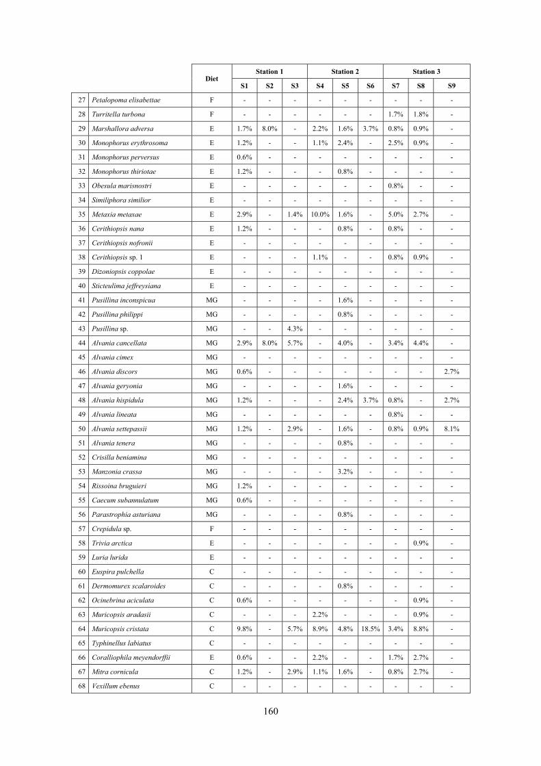
160

Diet Station 1 Station 2 Station 3

S1 S2 S3 S4 S5 S6 S7 S8 S9

27 Petalopoma elisabettae F - - - - - - - - -

28 Turritella turbona F - - - - - - 1.7% 1.8% -

29 Marshallora adversa E 1.7% 8.0% - 2.2% 1.6% 3.7% 0.8% 0.9% -

30 Monophorus erythrosoma E 1.2% - - 1.1% 2.4% - 2.5% 0.9% -

31 Monophorus perversus E 0.6% - - - - - - - -

32 Monophorus thiriotae E 1.2% - - - 0.8% - - - -

33 Obesula marisnostri E - - - - - - 0.8% - -

34 Similiphora similior E - - - - - - - - -

35 Metaxia metaxae E 2.9% - 1.4% 10.0% 1.6% - 5.0% 2.7% -

36 Cerithiopsis nana E 1.2% - - - 0.8% - 0.8% - -

37 Cerithiopsis nofronii E - - - - - - - - -

38 Cerithiopsis sp. 1 E - - - 1.1% - - 0.8% 0.9% -

39 Dizoniopsis coppolae E - - - - - - - - -

40 Sticteulima jeffreysiana E - - - - - - - - -

41 Pusillina inconspicua MG - - - - 1.6% - - - -

42 Pusillina philippi MG - - - - 0.8% - - - -

43 Pusillina sp. MG - - 4.3% - - - - - -

44 Alvania cancellata MG 2.9% 8.0% 5.7% - 4.0% - 3.4% 4.4% -

45 Alvania cimex MG - - - - - - - - -

46 Alvania discors MG 0.6% - - - - - - - 2.7% 47 Alvania geryonia MG - - - - 1.6% - - - -

48 Alvania hispidula MG 1.2% - - - 2.4% 3.7% 0.8% - 2.7% 49 Alvania lineata MG - - - - - - 0.8% - -

50 Alvania settepassii MG 1.2% - 2.9% - 1.6% - 0.8% 0.9% 8.1% 51 Alvania tenera MG - - - - 0.8% - - - -

52 Crisilla beniamina MG - - - - - - - - -

53 Manzonia crassa MG - - - - 3.2% - - - -

54 Rissoina bruguieri MG 1.2% - - - - - - - -

55 Caecum subannulatum MG 0.6% - - - - - - - -

56 Parastrophia asturiana MG - - - - 0.8% - - - -

57 Crepidula sp. F - - - - - - - - -

58 Trivia arctica E - - - - - - - 0.9% -

59 Luria lurida E - - - - - - - - -

60 Euspira pulchella C - - - - - - - - -

61 Dermomurex scalaroides C - - - - 0.8% - - - -

62 Ocinebrina aciculata C 0.6% - - - - - - 0.9% -

63 Muricopsis aradasii C - - - 2.2% - - - 0.9% -

64 Muricopsis cristata C 9.8% - 5.7% 8.9% 4.8% 18.5% 3.4% 8.8% -

65 Typhinellus labiatus C - - - - - - - - -

66 Coralliophila meyendorffii E 0.6% - - 2.2% - - 1.7% 2.7% -

67 Mitra cornicula C 1.2% - 2.9% 1.1% 1.6% - 0.8% 2.7% -

68 Vexillum ebenus C - - - - - - - - -

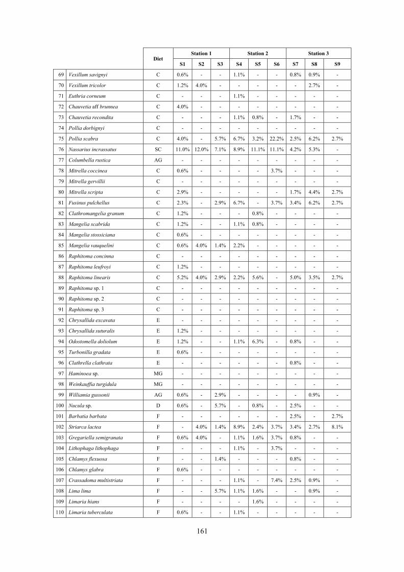
161

Diet Station 1 Station 2 Station 3

S1 S2 S3 S4 S5 S6 S7 S8 S9

69 Vexillum savignyi C 0.6% - - 1.1% - - 0.8% 0.9% -

70 Vexillum tricolor C 1.2% 4.0% - - - - - 2.7% -

71 Euthria corneum C - - - 1.1% - - - - -

72 Chauvetia aff brunnea C 4.0% - - - - - - - -

73 Chauvetia recondita C - - - 1.1% 0.8% - 1.7% - -

74 Pollia dorbignyi C - - - - - - - - -

75 Pollia scabra C 4.0% - 5.7% 6.7% 3.2% 22.2% 2.5% 6.2% 2.7%

76 Nassarius incrassatus SC 11.0% 12.0% 7.1% 8.9% 11.1% 11.1% 4.2% 5.3% -

77 Columbella rustica AG - - - - - - - - -

78 Mitrella coccinea C 0.6% - - - - 3.7% - - -

79 Mitrella gervillii C - - - - - - - - -

80 Mitrella scripta C 2.9% - - - - - 1.7% 4.4% 2.7%

81 Fusinus pulchellus C 2.3% - 2.9% 6.7% - 3.7% 3.4% 6.2% 2.7%

82 Clathromangelia granum C 1.2% - - - 0.8% - - - -

83 Mangelia scabrida C 1.2% - - 1.1% 0.8% - - - -

84 Mangelia stossiciana C 0.6% - - - - - - - -

85 Mangelia vauquelini C 0.6% 4.0% 1.4% 2.2% - - - - -

86 Raphitoma concinna C - - - - - - - - -

87 Raphitoma leufroyi C 1.2% - - - - - - - -

88 Raphitoma linearis C 5.2% 4.0% 2.9% 2.2% 5.6% - 5.0% 3.5% 2.7% 89 Raphitoma sp. 1 C - - - - - - - - -

90 Raphitoma sp. 2 C - - - - - - - - -

91 Raphitoma sp. 3 C - - - - - - - - -

92 Chrysallida excavata E - - - - - - - - -

93 Chrysallida suturalis E 1.2% - - - - - - - -

94 Odostomella doliolum E 1.2% - - 1.1% 6.3% - 0.8% - -

95 Turbonilla gradata E 0.6% - - - - - - - -

96 Clathrella clathrata E - - - - - - 0.8% - -

97 Haminoea sp. MG - - - - - - - - -

98 Weinkauffia turgidula MG - - - - - - - - -

99 Williamia gussonii AG 0.6% - 2.9% - - - - 0.9% -

100 Nucula sp. D 0.6% - 5.7% - 0.8% - 2.5% - -

101 Barbatia barbata F - - - - - - 2.5% - 2.7% 102 Striarca lactea F - 4.0% 1.4% 8.9% 2.4% 3.7% 3.4% 2.7% 8.1% 103 Gregariella semigranata F 0.6% 4.0% - 1.1% 1.6% 3.7% 0.8% - -

104 Lithophaga lithophaga F - - - 1.1% - 3.7% - - -

105 Chlamys flexuosa F - - 1.4% - - - 0.8% - -

106 Chlamys glabra F 0.6% - - - - - - - -

107 Crassadoma multistriata F - - - 1.1% - 7.4% 2.5% 0.9% -

108 Lima lima F - - 5.7% 1.1% 1.6% - - 0.9% -

109 Limaria hians F - - - - 1.6% - - - -

110 Limaria tuberculata F 0.6% - - 1.1% - - - - -

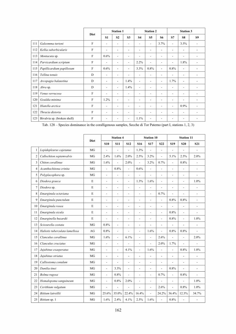
162

Diet Station 1 Station 2 Station 3

S1 S2 S3 S4 S5 S6 S7 S8 S9

111 Galeomma turtoni F - - - - - 3.7% - 3.5% -

112 Kellia suborbicularis F - - - - - - - - -

113 Montacuta sp. F 0.6% - - - - - - - -

114 Parvicardium scriptum F - - - 2.2% - - - 1.8% -

115 Papillicardium papillosum F 0.6% - - 3.3% 0.8% - 0.8% - -

116 Tellina tenuis D - - - - - - - - -

117 Arcopagia balaustina D - - 1.4% - - - 1.7% - -

118 Abra sp. D - - 1.4% - - - - - -

119 Venus verrucosa F - - - - - - - - - 120 Gouldia minima F 1.2% - - - - - - - -

121 Hiatella arctica F - - - - - - - 0.9% -

122 Thracia distorta F - - - - - - - - -

123 Bivalvia sp. (broken shell) F - - - 1.1% - - - - -

Tab. 128 – Species dominance in the coralligenous samples, Secche di Tor Paterno (part I, stations 1, 2, 3)

Diet

Station 4 Station 10 Station 11

S10 S11 S12 S16 S17 S22 S19 S20 S21

1 Lepidopleurus cajetanus MG - - - 1.3% - - - - - 2 Callochiton septemvalvis MG 2.4% 1.6% 2.0% 2.5% 3.2% - 5.1% 2.5% 2.0% 3 Chiton corallinus MG 1.6% - 2.0% - 3.2% 0.7% - 0.8% -

4 Acanthochitona crinita MG - 0.8% - 0.6% - - - - -

5 Polyplacophora sp. MG - - - - - - - - -

6 Diodora graeca E - - - 1.3% 1.6% - - - 1.0% 7 Diodora sp. E - - - - - - - - -

8 Emarginula octaviana E - - - - - 0.7% - - -

9 Emarginula punctulum E - - - - - - 0.8% 0.8% -

10 Emarginula rosea E - - - - - - - - -

11 Emarginula sicula E - - - - - - 0.8% - -

12 Emarginella huzardii E - - - - - - 0.8% - 1.0%

13 Scissurella costata MG 0.8% - - - - - - - -

14 Haliotis tuberculata lamellosa AG 0.8% - - - 1.6% - 0.8% 0.8% -

15 Clanculus corallinus MG 1.6% - 6.1% - - 2.6% - - 2.0% 16 Clanculus cruciatus MG - - - - - 2.0% 1.7% - -

17 Jujubinus exasperatus MG - - 4.1% - 1.6% - - 0.8% 1.0%

18 Jujubinus striatus MG - - - - - - - - -

19 Calliostoma conulum MG - - - - - - - - -

20 Danilia tinei MG - 3.3% - - - - 0.8% - -

21 Bolma rugosa MG - 0.8% - - - 0.7% - 0.8% -

22 Homalopoma sanguineum MG - 0.8% 2.0% - - - - - 1.0%

23 Cerithium vulgatum MG - - - - - 2.6% - 0.8% 1.0%

24 Bittium latreillii MG 25.6% 35.0% 22.4% 16.4% - 24.2% 36.4% 12.3% 34.7%

25 Bittium sp. 1 MG 1.6% 2.4% 4.1% 2.5% 1.6% - 0.8% - -

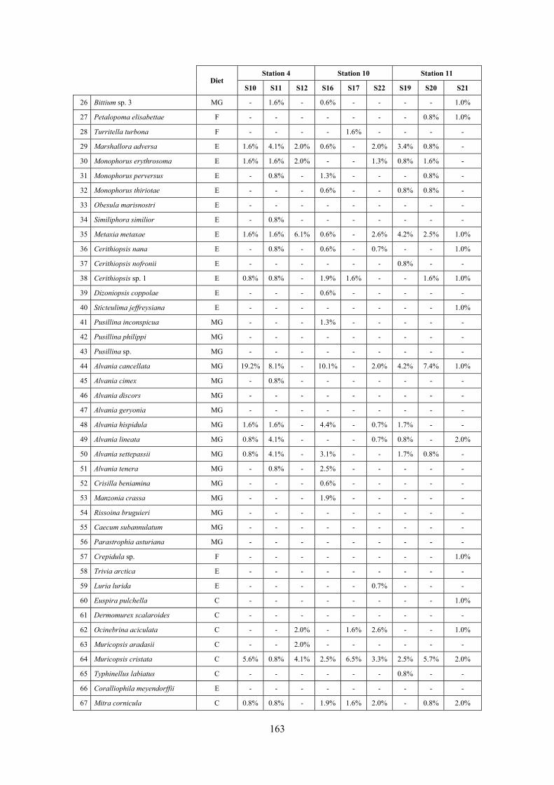
163

Diet Station 4 Station 10 Station 11

S10 S11 S12 S16 S17 S22 S19 S20 S21

26 Bittium sp. 3 MG - 1.6% - 0.6% - - - - 1.0%

27 Petalopoma elisabettae F - - - - - - - 0.8% 1.0%

28 Turritella turbona F - - - - 1.6% - - - -

29 Marshallora adversa E 1.6% 4.1% 2.0% 0.6% - 2.0% 3.4% 0.8% -

30 Monophorus erythrosoma E 1.6% 1.6% 2.0% - - 1.3% 0.8% 1.6% -

31 Monophorus perversus E - 0.8% - 1.3% - - - 0.8% -

32 Monophorus thiriotae E - - - 0.6% - - 0.8% 0.8% -

33 Obesula marisnostri E - - - - - - - - -

34 Similiphora similior E - 0.8% - - - - - - -

35 Metaxia metaxae E 1.6% 1.6% 6.1% 0.6% - 2.6% 4.2% 2.5% 1.0%

36 Cerithiopsis nana E - 0.8% - 0.6% - 0.7% - - 1.0% 37 Cerithiopsis nofronii E - - - - - - 0.8% - -

38 Cerithiopsis sp. 1 E 0.8% 0.8% - 1.9% 1.6% - - 1.6% 1.0% 39 Dizoniopsis coppolae E - - - 0.6% - - - - -

40 Sticteulima jeffreysiana E - - - - - - - - 1.0%

41 Pusillina inconspicua MG - - - 1.3% - - - - -

42 Pusillina philippi MG - - - - - - - - -

43 Pusillina sp. MG - - - - - - - - -

44 Alvania cancellata MG 19.2% 8.1% - 10.1% - 2.0% 4.2% 7.4% 1.0%

45 Alvania cimex MG - 0.8% - - - - - - -

46 Alvania discors MG - - - - - - - - -

47 Alvania geryonia MG - - - - - - - - -

48 Alvania hispidula MG 1.6% 1.6% - 4.4% - 0.7% 1.7% - -

49 Alvania lineata MG 0.8% 4.1% - - - 0.7% 0.8% - 2.0% 50 Alvania settepassii MG 0.8% 4.1% - 3.1% - - 1.7% 0.8% -

51 Alvania tenera MG - 0.8% - 2.5% - - - - -

52 Crisilla beniamina MG - - - 0.6% - - - - -

53 Manzonia crassa MG - - - 1.9% - - - - -

54 Rissoina bruguieri MG - - - - - - - - -

55 Caecum subannulatum MG - - - - - - - - -

56 Parastrophia asturiana MG - - - - - - - - -

57 Crepidula sp. F - - - - - - - - 1.0%

58 Trivia arctica E - - - - - - - - -

59 Luria lurida E - - - - - 0.7% - - -

60 Euspira pulchella C - - - - - - - - 1.0%

61 Dermomurex scalaroides C - - - - - - - - -

62 Ocinebrina aciculata C - - 2.0% - 1.6% 2.6% - - 1.0% 63 Muricopsis aradasii C - - 2.0% - - - - - -

64 Muricopsis cristata C 5.6% 0.8% 4.1% 2.5% 6.5% 3.3% 2.5% 5.7% 2.0% 65 Typhinellus labiatus C - - - - - - 0.8% - -

66 Coralliophila meyendorffii E - - - - - - - - -

67 Mitra cornicula C 0.8% 0.8% - 1.9% 1.6% 2.0% - 0.8% 2.0%

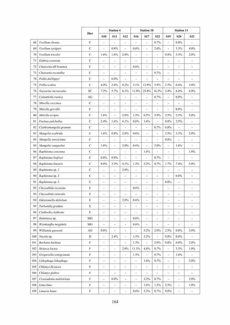
164

Diet Station 4 Station 10 Station 11

S10 S11 S12 S16 S17 S22 S19 S20 S21

68 Vexillum ebenus C - - - - - 0.7% - 0.8% -

69 Vexillum savignyi C - 0.8% - 0.6% - 2.0% - 3.3% 4.0% 70 Vexillum tricolor C 1.6% 1.6% 2.0% - - - 0.8% 3.3% 2.0%

71 Euthria corneum C - - - - - - - - -

72 Chauvetia aff brunnea C - - - 0.6% - - - - -

73 Chauvetia recondita C - - - - - 0.7% - - -

74 Pollia dorbignyi C - 0.8% - - - - - - -

75 Pollia scabra C 4.0% 2.4% 8.2% 3.1% 12.9% 3.9% 2.5% 6.6% 2.0%

76 Nassarius incrassatus SC 7.2% 5.7% 6.1% 11.9% 25.8% 16.3% 3.4% 6.6% 6.9%

77 Columbella rustica AG - - - - - 0.7% - 0.8% -

78 Mitrella coccinea C - - - - - - - - -

79 Mitrella gervillii C - - - - - - - 0.8% -

80 Mitrella scripta C 1.6% - 2.0% 1.3% 6.5% 5.9% 2.5% 2.5% 5.0%

81 Fusinus pulchellus C 2.4% 1.6% 4.1% 0.6% 1.6% - 0.8% 2.5% -

82 Clathromangelia granum C - - - - - 0.7% 0.8% - -

83 Mangelia scabrida C 1.6% 0.8% 2.0% 0.6% - - 2.5% 3.3% 2.0% 84 Mangelia stossiciana C - - - - - - 0.8% - -

85 Mangelia vauquelini C 1.6% - 2.0% 0.6% - 2.0% - 1.6% -

86 Raphitoma concinna C - - - - 1.6% - - - 1.0% 87 Raphitoma leufroyi C 0.8% 0.8% - - - 0.7% - - -

88 Raphitoma linearis C 8.0% 3.3% 4.1% 1.3% 3.2% 0.7% 1.7% 7.4% 5.0% 89 Raphitoma sp. 1 C - - 2.0% - - - - - -

90 Raphitoma sp. 2 C - - - - - - - 0.8% -

91 Raphitoma sp. 3 C - - - - - - 0.8% - -

92 Chrysallida excavata E - - - 0.6% - - - - -

93 Chrysallida suturalis E - - - - - - - - -

94 Odostomella doliolum E - - 2.0% 0.6% - - - - -

95 Turbonilla gradata E - - - - - - - - -

96 Clathrella clathrata E - - - - - - - - -

97 Haminoea sp. MG - - - 0.6% - - - - -

98 Weinkauffia turgidula MG - - - 0.6% - - - - -

99 Williamia gussonii AG 0.8% - - - 3.2% 2.0% 2.5% 0.8% 3.0%

100 Nucula sp. D - 2.4% - 1.3% 3.2% - 0.8% 0.8% -

101 Barbatia barbata F - - - 1.3% - 2.0% 0.8% 0.8% 2.0% 102 Striarca lactea F - - 2.0% 11.3% 4.8% 0.7% - 3.3% 1.0% 103 Gregariella semigranata F - - - 1.3% - 0.7% - 1.6% - 104 Lithophaga lithophaga F - - - - 1.6% 0.7% - - 2.0% 105 Chlamys flexuosa F - - - - - - - - -

106 Chlamys glabra F - - - - - - - - -

107 Crassadoma multistriata F - 0.8% - - 3.2% 0.7% - - 2.0% 108 Lima lima F - - - - 1.6% 1.3% 2.5% - 1.0% 109 Limaria hians F - - - 0.6% 3.2% 0.7% 0.8% - -

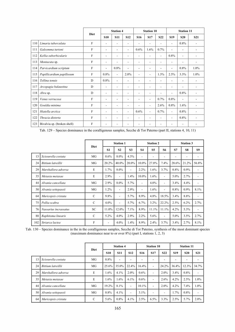
165

Diet Station 4 Station 10 Station 11

S10 S11 S12 S16 S17 S22 S19 S20 S21

110 Limaria tuberculata F - - - - - - - 0.8% -

111 Galeomma turtoni F - - - 0.6% 1.6% 0.7% - - -

112 Kellia suborbicularis F - - - - - - 0.8% - -

113 Montacuta sp. F - - - - - - - - -

114 Parvicardium scriptum F - 0.8% - - - - - 0.8% 1.0% 115 Papillicardium papillosum F 0.8% - 2.0% - - 1.3% 2.5% 3.3% 1.0%

116 Tellina tenuis D 0.8% - - - - - - - -

117 Arcopagia balaustina D - - - - - - - - -

118 Abra sp. D - - - - - - - 0.8% -

119 Venus verrucosa F - - - - - 0.7% 0.8% - -

120 Gouldia minima F - - - - - 2.6% 0.8% 1.6% -

121 Hiatella arctica F - - - 0.6% - 0.7% - 0.8% -

122 Thracia distorta F - - - - - - - 0.8% -

123 Bivalvia sp. (broken shell) F - - - - - - - - -

Tab. 129 – Species dominance in the coralligenous samples, Secche di Tor Paterno (part II, stations 4, 10, 11)

  Diet

Station 1 Station 2 Station 3

S1 S2 S3 S4 S5 S6 S7 S8 S9

13 Scissurella costata MG 0.6% 8.0% 4.3% - - - - - -

24 Bittium latreillii MG 20.2% 40.0% 20.0% 10.0% 27.8% 7.4% 28.6% 21.2% 56.8%

29 Marshallora adversa E 1.7% 8.0% - 2.2% 1.6% 3.7% 0.8% 0.9% -

35 Metaxia metaxae E 2.9% - 1.4% 10.0% 1.6% - 5.0% 2.7% -

44 Alvania cancellata MG 2.9% 8.0% 5.7% - 4.0% - 3.4% 4.4% -

50 Alvania settepassii MG 1.2% - 2.9% - 1.6% - 0.8% 0.9% 8.1%

64 Muricopsis cristata C 9.8% - 5.7% 8.9% 4.8% 18.5% 3.4% 8.8% -

75 Pollia scabra C 4.0% - 5.7% 6.7% 3.2% 22.2% 2.5% 6.2% 2.7%

76 Nassarius incrassatus SC 11.0% 12.0% 7.1% 8.9% 11.1% 11.1% 4.2% 5.3% -

88 Raphitoma linearis C 5.2% 4.0% 2.9% 2.2% 5.6% - 5.0% 3.5% 2.7%

102 Striarca lactea F - 4.0% 1.4% 8.9% 2.4% 3.7% 3.4% 2.7% 8.1%

Tab. 130 – Species dominance in the in the coralligenous samples, Secche di Tor Paterno, synthesis of the most dominant species (maximum dominance near to or over 8%) (part I, stations 1, 2, 3)

  Diet

Station 4 Station 10 Station 11

S10 S11 S12 S16 S17 S22 S19 S20 S21

13 Scissurella costata MG 0.8% - - - - - - - -

24 Bittium latreillii MG 25.6% 35.0% 22.4% 16.4% - 24.2% 36.4% 12.3% 34.7%

29 Marshallora adversa E 1.6% 4.1% 2.0% 0.6% - 2.0% 3.4% 0.8% -

35 Metaxia metaxae E 1.6% 1.6% 6.1% 0.6% - 2.6% 4.2% 2.5% 1.0%

44 Alvania cancellata MG 19.2% 8.1% - 10.1% - 2.0% 4.2% 7.4% 1.0%

50 Alvania settepassii MG 0.8% 4.1% - 3.1% - - 1.7% 0.8% -

64 Muricopsis cristata C 5.6% 0.8% 4.1% 2.5% 6.5% 3.3% 2.5% 5.7% 2.0%

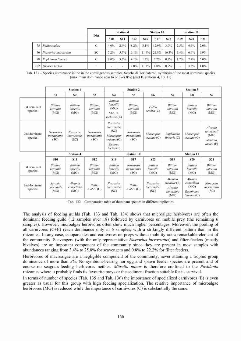
166

  Diet

Station 4 Station 10 Station 11

S10 S11 S12 S16 S17 S22 S19 S20 S21

75 Pollia scabra C 4.0% 2.4% 8.2% 3.1% 12.9% 3.9% 2.5% 6.6% 2.0%

76 Nassarius incrassatus SC 7.2% 5.7% 6.1% 11.9% 25.8% 16.3% 3.4% 6.6% 6.9%

88 Raphitoma linearis C 8.0% 3.3% 4.1% 1.3% 3.2% 0.7% 1.7% 7.4% 5.0%

102 Striarca lactea F - - 2.0% 11.3% 4.8% 0.7% - 3.3% 1.0%

Tab. 131 – Species dominance in the in the coralligenous samples, Secche di Tor Paterno, synthesis of the most dominant species (maximum dominance near to or over 8%) (part II, stations 4, 10, 11)

Station 1 Station 2 Station 3 S1 S2 S3 S4 S5 S6 S7 S8 S9

1st dominant species

Bittium latreillii (MG)

Bittium latreillii (MG)

Bittium latreillii (MG)

Bittium latreillii (MG)

Metaxia metaxae (E)

Bittium latreillii (MG)

Pollia scabra (C)

Bittium latreillii (MG)

Bittium latreillii (MG)

Bittium latreillii (MG)

2nd dominant species

Nassarius incrassatus

(SC)

Nassarius incrassatus

(SC)

Nassarius incrassatus

(SC)

Nassarius incrassatus

(SC) Muricopsis cristata (C)

Striarca lactea (F)

Nassarius incrassatus

(SC)

Muricopsis cristata (C)

Raphitoma linearis (C)

Muricopsis cristata (C)

Alvania settepassii

(MG) Striarca

lactea (F)

Station 4 Station 10 Station 11 S10 S11 S12 S16 S17 S22 S19 S20 S21

1st dominant species

Bittium latreillii (MG)

Bittium latreillii (MG)

Bittium latreillii (MG)

Bittium latreillii (MG)

Nassarius incrassatus

(SG)

Bittium latreillii (MG)

Bittium latreillii (MG)

Bittium latreillii (MG)

Bittium latreillii (MG)

2nd dominant species

Alvania cancellata

(MG)

Alvania cancellata

(MG)

Pollia scabra (C)

Nassarius incrassatus

(SC)

Pollia scabra (C)

Nassarius incrassatus

(SC)

Metaxia metaxae (E)

Alvania cancellata

(MG)

Alvania cancellata

(MG) Raphitoma linearis (C)

Nassarius incrassatus

(SC)

Tab. 132 – Comparative table of dominant species in different replicates

The analysis of feeding guilds (Tab. 133 and Tab. 134) shows that microalgae herbivores are often the dominant feeding guild (12 samples over 18) followed by carnivores on mobile prey (the remaining 6 samples). However, microalgae herbivores often show much higher percentages. Moreover, the pooling of all carnivores (C+E) reach dominance only in 6 samples, with a strikingly different pattern than in the rhizomes. In any case, ectoparasites and carnivores on preys without mobility are a remarkable element of the community. Scavengers (with the only representative Nassarius incrassatus) and filter-feeders (mostly bivalves) are an important component of the community since they are present in most samples with abundances ranging from 3.4% to 25.8% for scavengers and 0.8% to 22.2% for filter feeders. Herbivores of macroalgae are a negligible component of the community, never attaining a trophic group dominance of more than 5%. No symbiont-bearing nor egg and spawn feeder species are present and of course no seagrass-feeding herbivores neither. Mitrella minor is therefore confined to the Posidonia rhizomes where it probably finds its favourite preys or the sediment fraction suitable for its survival. In terms of number of species (Tab. 135 and Tab. 136) the importance of specialized carnivores (E) is even greater as usual for this group with high feeding specialization. The relative importance of microalgae herbivores (MG) is reduced while the importance of carnivores (C) is substantially the same.

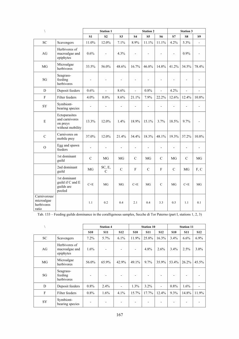
167

\

Station 1 Station 2 Station 3

S1 S2 S3 S4 S5 S6 S7 S8 S9

SC Scavengers 11.0% 12.0% 7.1% 8.9% 11.1% 11.1% 4.2% 5.3% -

AG Herbivores of macroalgae and epiphytes

0.6% - 4.3% - - - - 0.9% -

MG Microalgae herbivores 33.5% 56.0% 48.6% 16.7% 46.8% 14.8% 41.2% 34.5% 78.4%

SG Seagrass-feeding herbivores

- - - - - - - - -

D Deposit feeders 0.6% - 8.6% - 0.8% - 4.2% - -

F Filter feeders 4.0% 8.0% 8.6% 21.1% 7.9% 22.2% 12.6% 12.4% 10.8%

SY Symbiont-bearing species - - - - - - - - -

E

Ectoparasites and carnivores on preys without mobility

13.3% 12.0% 1.4% 18.9% 15.1% 3.7% 18.5% 9.7% -

C Carnivores on mobile prey 37.0% 12.0% 21.4% 34.4% 18.3% 48.1% 19.3% 37.2% 10.8%

O Egg and spawn feeders - - - - - - - - -

1st dominant guild C MG MG C MG C MG C MG

2nd dominant guild MG SC, E,

C C F C F C MG F, C

1st dominant guild if C and E guilds are pooled

C+E MG MG C+E MG C MG C+E MG

Carnivorous/ microalgae herbivores ratio

1.1 0.2 0.4 2.1 0.4 3.3 0.5 1.1 0.1

Tab. 133 – Feeding guilds dominance in the coralligenous samples, Secche di Tor Paterno (part I, stations 1, 2, 3)

\

Station 4 Station 10 Station 11

S10 S11 S12 S10 S11 S12 S10 S11 S12

SC Scavengers 7.2% 5.7% 6.1% 11.9% 25.8% 16.3% 3.4% 6.6% 6.9%

AG Herbivores of macroalgae and epiphytes

1.6% - - - 4.8% 2.6% 3.4% 2.5% 3.0%

MG Microalgae herbivores 56.0% 65.9% 42.9% 49.1% 9.7% 35.9% 53.4% 26.2% 45.5%

SG Seagrass-feeding herbivores

- - - - - - - - -

D Deposit feeders 0.8% 2.4% - 1.3% 3.2% - 0.8% 1.6% -

F Filter feeders 0.8% 1.6% 4.1% 15.7% 17.7% 12.4% 9.3% 14.8% 11.9%

SY Symbiont-bearing species - - - - - - - - -

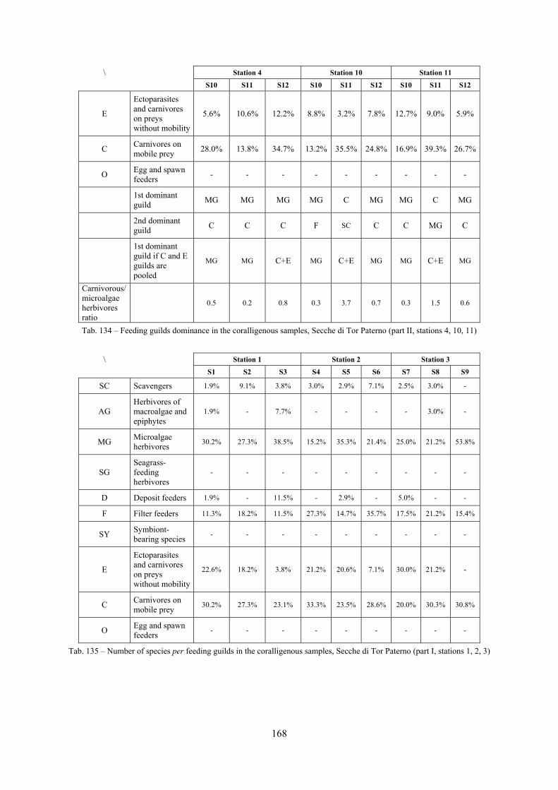
168

\

Station 4 Station 10 Station 11

S10 S11 S12 S10 S11 S12 S10 S11 S12

E

Ectoparasites and carnivores on preys without mobility

5.6% 10.6% 12.2% 8.8% 3.2% 7.8% 12.7% 9.0% 5.9%

C Carnivores on mobile prey 28.0% 13.8% 34.7% 13.2% 35.5% 24.8% 16.9% 39.3% 26.7%

O Egg and spawn feeders - - - - - - - - -

1st dominant guild MG MG MG MG C MG MG C MG

2nd dominant guild C C C F SC C C MG C

1st dominant guild if C and E guilds are pooled

MG MG C+E MG C+E MG MG C+E MG

Carnivorous/ microalgae herbivores ratio

0.5 0.2 0.8 0.3 3.7 0.7 0.3 1.5 0.6

Tab. 134 – Feeding guilds dominance in the coralligenous samples, Secche di Tor Paterno (part II, stations 4, 10, 11)

\

Station 1 Station 2 Station 3

S1 S2 S3 S4 S5 S6 S7 S8 S9

SC Scavengers 1.9% 9.1% 3.8% 3.0% 2.9% 7.1% 2.5% 3.0% -

AG Herbivores of macroalgae and epiphytes

1.9% - 7.7% - - - - 3.0% -

MG Microalgae herbivores 30.2% 27.3% 38.5% 15.2% 35.3% 21.4% 25.0% 21.2% 53.8%

SG Seagrass-feeding herbivores

- - - - - - - - -

D Deposit feeders 1.9% - 11.5% - 2.9% - 5.0% - -

F Filter feeders 11.3% 18.2% 11.5% 27.3% 14.7% 35.7% 17.5% 21.2% 15.4%

SY Symbiont-bearing species - - - - - - - - -

E

Ectoparasites and carnivores on preys without mobility

22.6% 18.2% 3.8% 21.2% 20.6% 7.1% 30.0% 21.2% -

C Carnivores on mobile prey 30.2% 27.3% 23.1% 33.3% 23.5% 28.6% 20.0% 30.3% 30.8%

O Egg and spawn feeders - - - - - - - - -

Tab. 135 – Number of species per feeding guilds in the coralligenous samples, Secche di Tor Paterno (part I, stations 1, 2, 3)

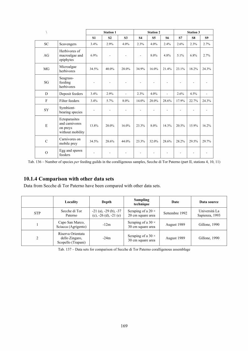
169

\

Station 1 Station 2 Station 3

S1 S2 S3 S4 S5 S6 S7 S8 S9

SC Scavengers 3.4% 2.9% 4.0% 2.3% 4.0% 2.4% 2.6% 2.3% 2.7%

AG Herbivores of macroalgae and epiphytes

6.9% - - - 8.0% 4.8% 5.1% 6.8% 2.7%

MG Microalgae herbivores 34.5% 40.0% 28.0% 34.9% 16.0% 21.4% 23.1% 18.2% 24.3%

SG Seagrass-feeding herbivores

- - - - - - - - -

D Deposit feeders 3.4% 2.9% - 2.3% 4.0% - 2.6% 4.5% -

F Filter feeders 3.4% 5.7% 8.0% 14.0% 28.0% 28.6% 17.9% 22.7% 24.3%

SY Symbiont-bearing species - - - - - - - - -

E

Ectoparasites and carnivores on preys without mobility

13.8% 20.0% 16.0% 23.3% 8.0% 14.3% 20.5% 15.9% 16.2%

C Carnivores on mobile prey 34.5% 28.6% 44.0% 23.3% 32.0% 28.6% 28.2% 29.5% 29.7%

O Egg and spawn feeders - - - - - - - - -

Tab. 136 – Number of species per feeding guilds in the coralligenous samples, Secche di Tor Paterno (part II, stations 4, 10, 11)

10.1.4 Comparison with other data sets Data from Secche di Tor Paterno have been compared with other data sets.

Locality Depth Sampling technique Date Data source

STP Secche di Tor Paterno

-21 (a), -29 (b), -37 (c), -26 (d), -21 (e)

Scraping of a 20 × 20 cm square area Settembre 1992 Università La

Sapienza, 1993

1 Capo San Marco, Sciacca (Agrigento) -12m Scraping of a 30 ×

30 cm square area August 1989 Gillone, 1990

2 Riserva Orientata

dello Zingaro, Scopello (Trapani)

-24m Scraping of a 30 × 30 cm square area August 1989 Gillone, 1990

Tab. 137 – Data sets for comparison of Secche di Tor Paterno coralligenous assemblage

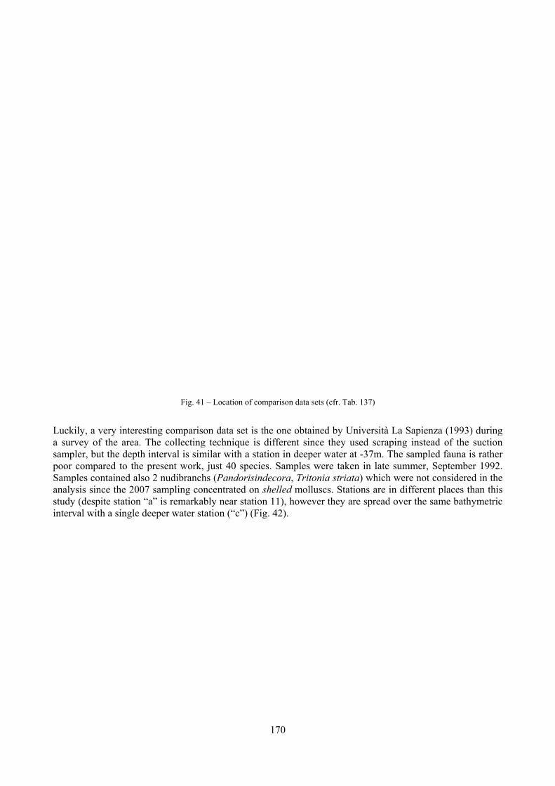
Luckily, a va survey ofsampler, bupoor compaSamples conanalysis sinstudy (despinterval with

very interestif the area. Tut the depth iared to the pntained also

nce the 2007 ite station “ah a single de

Fig. 4

ing comparisThe collectinginterval is simpresent work

2 nudibrancsampling co

a” is remarkaeeper water s

1 – Location of

son data setg technique milar with a

k, just 40 spechs (Pandorisoncentrated oably near stastation (“c”) (

170

f comparison da

is the one obis different station in de

ecies. Samplsindecora, Ton shelled mation 11), how(Fig. 42).

ata sets (cfr. Tab

btained by Usince they u

eeper water ales were takeTritonia striamolluscs. Statwever they a

b. 137)

Università Laused scrapinat -37m. Theen in late suta) which wetions are in dare spread ov

a Sapienza (1ng instead ofe sampled fauummer, Septeere not considifferent placver the same

1993) duringf the suctionuna is ratherember 1992.idered in theces than thisbathymetric

g n r . e s c

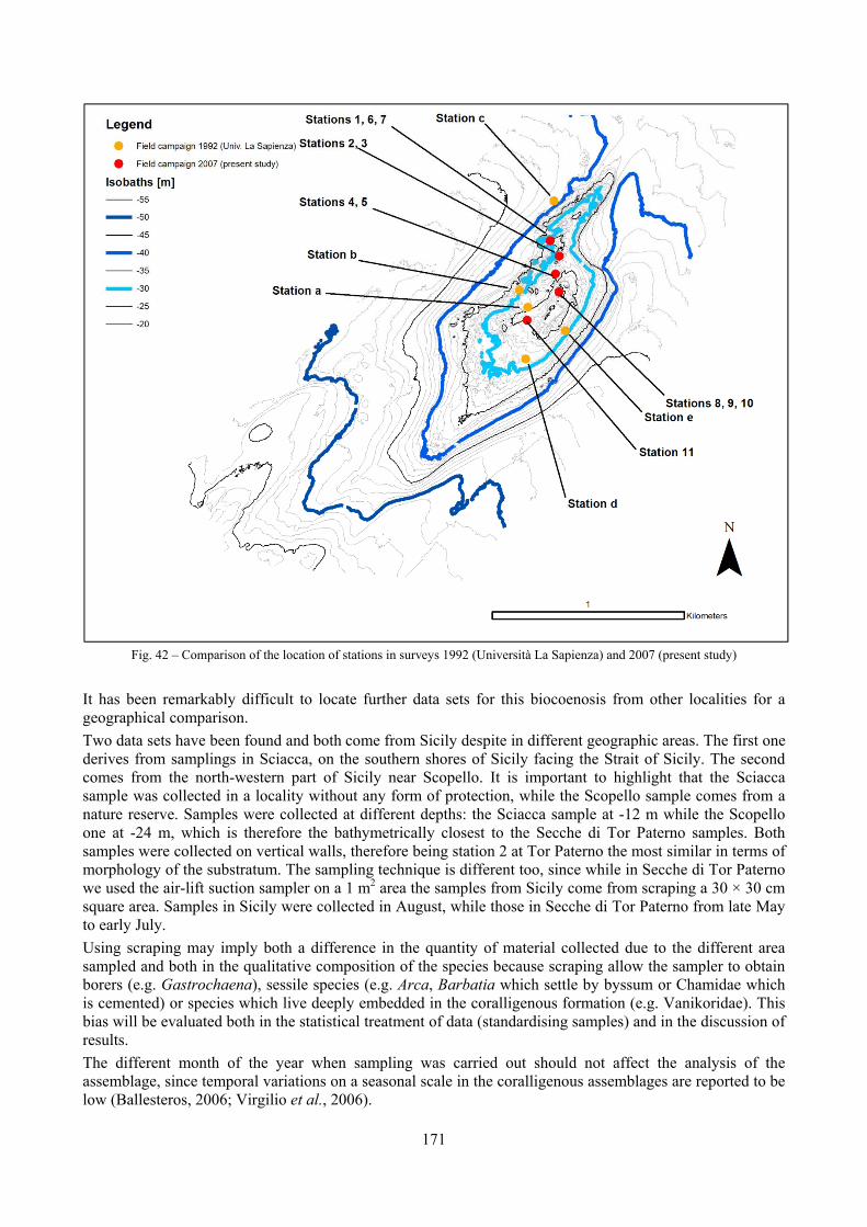
171

Fig. 42 – Comparison of the location of stations in surveys 1992 (Università La Sapienza) and 2007 (present study)

It has been remarkably difficult to locate further data sets for this biocoenosis from other localities for a geographical comparison. Two data sets have been found and both come from Sicily despite in different geographic areas. The first one derives from samplings in Sciacca, on the southern shores of Sicily facing the Strait of Sicily. The second comes from the north-western part of Sicily near Scopello. It is important to highlight that the Sciacca sample was collected in a locality without any form of protection, while the Scopello sample comes from a nature reserve. Samples were collected at different depths: the Sciacca sample at -12 m while the Scopello one at -24 m, which is therefore the bathymetrically closest to the Secche di Tor Paterno samples. Both samples were collected on vertical walls, therefore being station 2 at Tor Paterno the most similar in terms of morphology of the substratum. The sampling technique is different too, since while in Secche di Tor Paterno we used the air-lift suction sampler on a 1 m2 area the samples from Sicily come from scraping a 30 × 30 cm square area. Samples in Sicily were collected in August, while those in Secche di Tor Paterno from late May to early July. Using scraping may imply both a difference in the quantity of material collected due to the different area sampled and both in the qualitative composition of the species because scraping allow the sampler to obtain borers (e.g. Gastrochaena), sessile species (e.g. Arca, Barbatia which settle by byssum or Chamidae which is cemented) or species which live deeply embedded in the coralligenous formation (e.g. Vanikoridae). This bias will be evaluated both in the statistical treatment of data (standardising samples) and in the discussion of results. The different month of the year when sampling was carried out should not affect the analysis of the assemblage, since temporal variations on a seasonal scale in the coralligenous assemblages are reported to be low (Ballesteros, 2006; Virgilio et al., 2006).

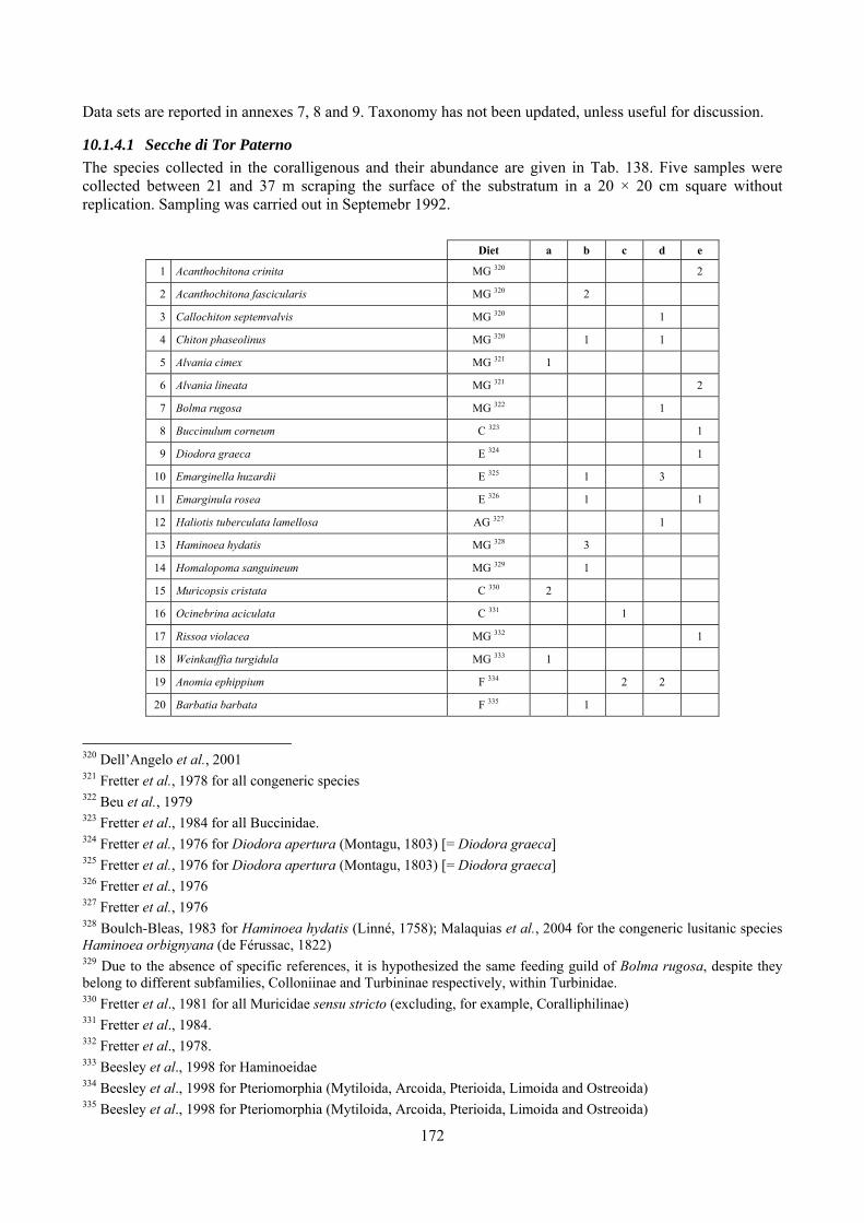
172

Data sets are reported in annexes 7, 8 and 9. Taxonomy has not been updated, unless useful for discussion.

10.1.4.1 Secche di Tor Paterno The species collected in the coralligenous and their abundance are given in Tab. 138. Five samples were collected between 21 and 37 m scraping the surface of the substratum in a 20 × 20 cm square without replication. Sampling was carried out in Septemebr 1992.

Diet a b c d e

1 Acanthochitona crinita MG 320 2

2 Acanthochitona fascicularis MG 320 2 3 Callochiton septemvalvis MG 320 1 4 Chiton phaseolinus MG 320 1 1 5 Alvania cimex MG 321 1 6 Alvania lineata MG 321 2

7 Bolma rugosa MG 322 1 8 Buccinulum corneum C 323 1

9 Diodora graeca E 324 1

10 Emarginella huzardii E 325 1 3 11 Emarginula rosea E 326 1 1

12 Haliotis tuberculata lamellosa AG 327 1 13 Haminoea hydatis MG 328 3 14 Homalopoma sanguineum MG 329 1 15 Muricopsis cristata C 330 2 16 Ocinebrina aciculata C 331 1 17 Rissoa violacea MG 332 1

18 Weinkauffia turgidula MG 333 1 19 Anomia ephippium F 334 2 2 20 Barbatia barbata F 335 1

320 Dell’Angelo et al., 2001 321 Fretter et al., 1978 for all congeneric species 322 Beu et al., 1979 323 Fretter et al., 1984 for all Buccinidae. 324 Fretter et al., 1976 for Diodora apertura (Montagu, 1803) [= Diodora graeca] 325 Fretter et al., 1976 for Diodora apertura (Montagu, 1803) [= Diodora graeca] 326 Fretter et al., 1976 327 Fretter et al., 1976 328 Boulch-Bleas, 1983 for Haminoea hydatis (Linné, 1758); Malaquias et al., 2004 for the congeneric lusitanic species Haminoea orbignyana (de Férussac, 1822) 329 Due to the absence of specific references, it is hypothesized the same feeding guild of Bolma rugosa, despite they belong to different subfamilies, Colloniinae and Turbininae respectively, within Turbinidae. 330 Fretter et al., 1981 for all Muricidae sensu stricto (excluding, for example, Coralliphilinae) 331 Fretter et al., 1984. 332 Fretter et al., 1978. 333 Beesley et al., 1998 for Haminoeidae 334 Beesley et al., 1998 for Pteriomorphia (Mytiloida, Arcoida, Pterioida, Limoida and Ostreoida) 335 Beesley et al., 1998 for Pteriomorphia (Mytiloida, Arcoida, Pterioida, Limoida and Ostreoida)

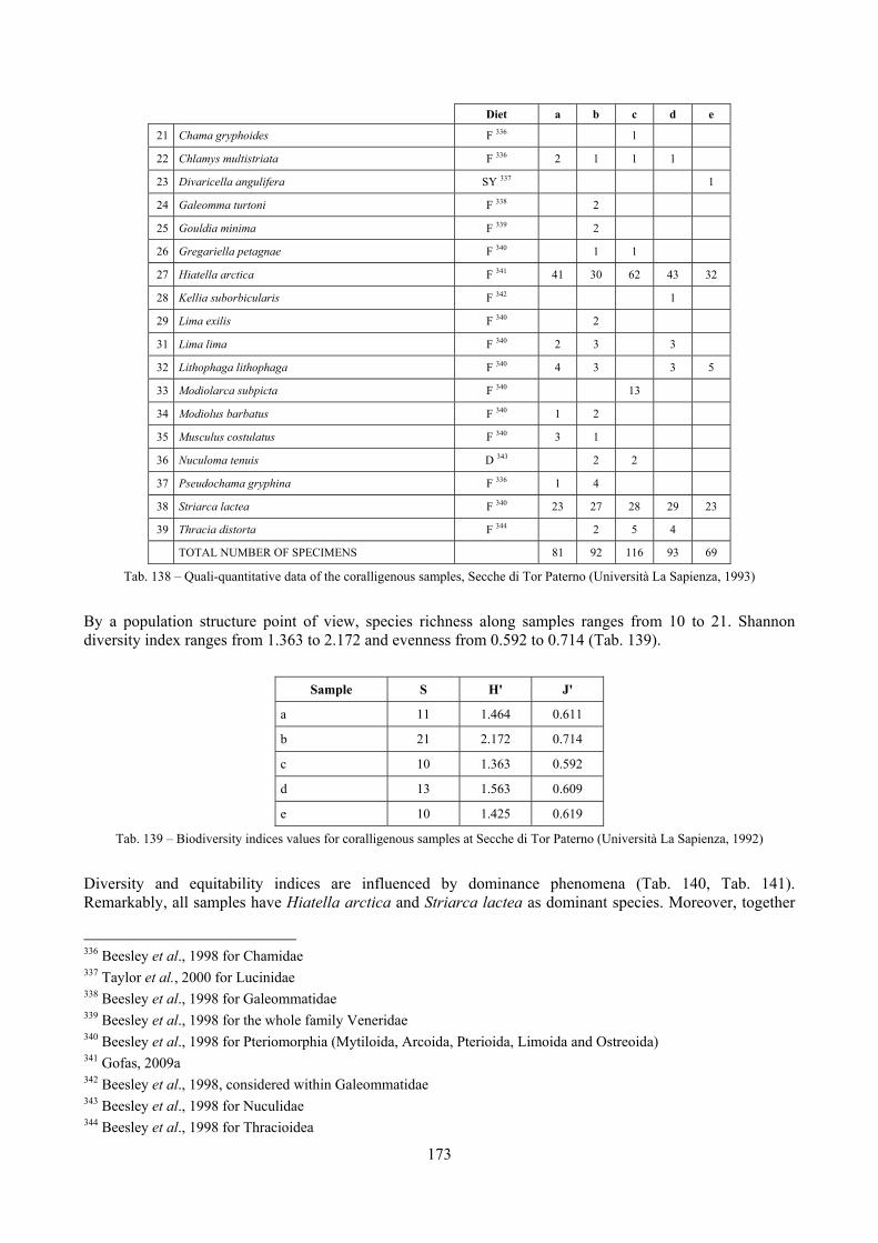
173

Diet a b c d e

21 Chama gryphoides F 336 1 22 Chlamys multistriata F 336 2 1 1 1 23 Divaricella angulifera SY 337 1

24 Galeomma turtoni F 338 2 25 Gouldia minima F 339 2 26 Gregariella petagnae F 340 1 1 27 Hiatella arctica F 341 41 30 62 43 32

28 Kellia suborbicularis F 342 1 29 Lima exilis F 340 2 31 Lima lima F 340 2 3 3 32 Lithophaga lithophaga F 340 4 3 3 5

33 Modiolarca subpicta F 340 13 34 Modiolus barbatus F 340 1 2 35 Musculus costulatus F 340 3 1 36 Nuculoma tenuis D 343 2 2 37 Pseudochama gryphina F 336 1 4 38 Striarca lactea F 340 23 27 28 29 23

39 Thracia distorta F 344 2 5 4 TOTAL NUMBER OF SPECIMENS 81 92 116 93 69

Tab. 138 – Quali-quantitative data of the coralligenous samples, Secche di Tor Paterno (Università La Sapienza, 1993)

By a population structure point of view, species richness along samples ranges from 10 to 21. Shannon diversity index ranges from 1.363 to 2.172 and evenness from 0.592 to 0.714 (Tab. 139).

Sample S H' J'

a 11 1.464 0.611

b 21 2.172 0.714

c 10 1.363 0.592

d 13 1.563 0.609

e 10 1.425 0.619

Tab. 139 – Biodiversity indices values for coralligenous samples at Secche di Tor Paterno (Università La Sapienza, 1992)

Diversity and equitability indices are influenced by dominance phenomena (Tab. 140, Tab. 141). Remarkably, all samples have Hiatella arctica and Striarca lactea as dominant species. Moreover, together

336 Beesley et al., 1998 for Chamidae 337 Taylor et al., 2000 for Lucinidae 338 Beesley et al., 1998 for Galeommatidae 339 Beesley et al., 1998 for the whole family Veneridae 340 Beesley et al., 1998 for Pteriomorphia (Mytiloida, Arcoida, Pterioida, Limoida and Ostreoida) 341 Gofas, 2009a 342 Beesley et al., 1998, considered within Galeommatidae 343 Beesley et al., 1998 for Nuculidae 344 Beesley et al., 1998 for Thracioidea

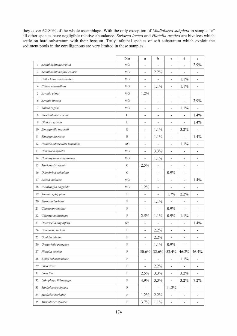
174

they cover 62-80% of the whole assemblage. With the only exception of Modiolarca subpicta in sample “c” all other species have negligible relative abundance. Striarca lactea and Hiatella arctica are bivalves which settle on hard substratum with their byssum. Truly infaunal species of soft substratum which exploit the sediment pools in the coralligenous are very limited in these samples.

Diet a b c d e

1 Acanthochitona crinita MG - - - - 2.9%

2 Acanthochitona fascicularis MG - 2.2% - - -

3 Callochiton septemvalvis MG - - - 1.1% -

4 Chiton phaseolinus MG - 1.1% - 1.1% -

5 Alvania cimex MG 1.2% - - - -

6 Alvania lineata MG - - - - 2.9%

7 Bolma rugosa MG - - - 1.1% -

8 Buccinulum corneum C - - - - 1.4%

9 Diodora graeca E - - - - 1.4%

10 Emarginella huzardii E - 1.1% - 3.2% -

11 Emarginula rosea E - 1.1% - - 1.4%

12 Haliotis tuberculata lamellosa AG - - - 1.1% -

13 Haminoea hydatis MG - 3.3% - - -

14 Homalopoma sanguineum MG - 1.1% - - -

15 Muricopsis cristata C 2.5% - - - -

16 Ocinebrina aciculata C - - 0.9% - -

17 Rissoa violacea MG - - - - 1.4%

18 Weinkauffia turgidula MG 1.2% - - - -

19 Anomia ephippium F - - 1.7% 2.2% -

20 Barbatia barbata F - 1.1% - - -

21 Chama gryphoides F - - 0.9% - -

22 Chlamys multistriata F 2.5% 1.1% 0.9% 1.1% -

23 Divaricella angulifera SY - - - - 1.4%

24 Galeomma turtoni F - 2.2% - - -

25 Gouldia minima F - 2.2% - - -

26 Gregariella petagnae F - 1.1% 0.9% - -

27 Hiatella arctica F 50.6% 32.6% 53.4% 46.2% 46.4%

28 Kellia suborbicularis F - - - 1.1% -

29 Lima exilis F - 2.2% - - -

31 Lima lima F 2.5% 3.3% - 3.2% -

32 Lithophaga lithophaga F 4.9% 3.3% - 3.2% 7.2%

33 Modiolarca subpicta F - - 11.2% - -

34 Modiolus barbatus F 1.2% 2.2% - - -

35 Musculus costulatus F 3.7% 1.1% - - -

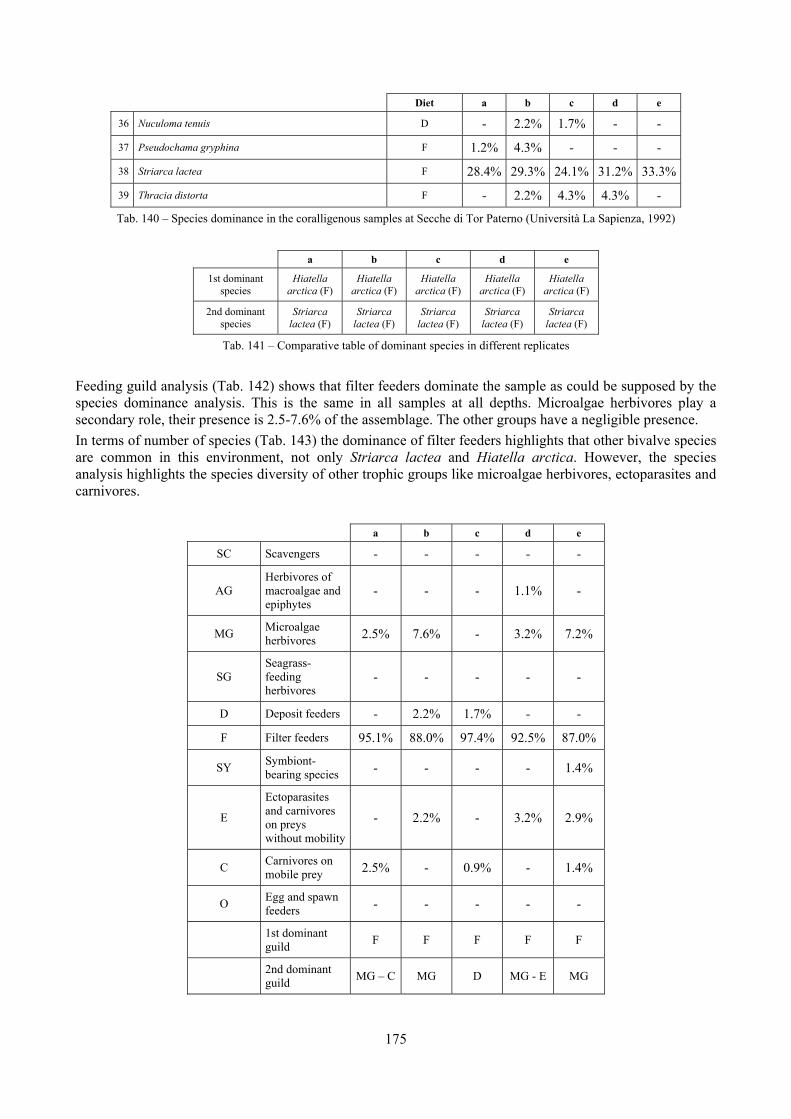
175

Diet a b c d e

36 Nuculoma tenuis D - 2.2% 1.7% - -

37 Pseudochama gryphina F 1.2% 4.3% - - -

38 Striarca lactea F 28.4% 29.3% 24.1% 31.2% 33.3%

39 Thracia distorta F - 2.2% 4.3% 4.3% -

Tab. 140 – Species dominance in the coralligenous samples at Secche di Tor Paterno (Università La Sapienza, 1992)

a b c d e

1st dominant species

Hiatella arctica (F)

Hiatella arctica (F)

Hiatella arctica (F)

Hiatella arctica (F)

Hiatella arctica (F)

2nd dominant species

Striarca lactea (F)

Striarca lactea (F)

Striarca lactea (F)

Striarca lactea (F)

Striarca lactea (F)

Tab. 141 – Comparative table of dominant species in different replicates

Feeding guild analysis (Tab. 142) shows that filter feeders dominate the sample as could be supposed by the species dominance analysis. This is the same in all samples at all depths. Microalgae herbivores play a secondary role, their presence is 2.5-7.6% of the assemblage. The other groups have a negligible presence. In terms of number of species (Tab. 143) the dominance of filter feeders highlights that other bivalve species are common in this environment, not only Striarca lactea and Hiatella arctica. However, the species analysis highlights the species diversity of other trophic groups like microalgae herbivores, ectoparasites and carnivores.

a b c d e

SC Scavengers - - - - -

AG Herbivores of macroalgae and epiphytes

- - - 1.1% -

MG Microalgae herbivores 2.5% 7.6% - 3.2% 7.2%

SG Seagrass-feeding herbivores

- - - - -

D Deposit feeders - 2.2% 1.7% - -

F Filter feeders 95.1% 88.0% 97.4% 92.5% 87.0%

SY Symbiont-bearing species - - - - 1.4%

E

Ectoparasites and carnivores on preys without mobility

- 2.2% - 3.2% 2.9%

C Carnivores on mobile prey 2.5% - 0.9% - 1.4%

O Egg and spawn feeders - - - - -

1st dominant guild F F F F F

2nd dominant guild MG – C MG D MG - E MG

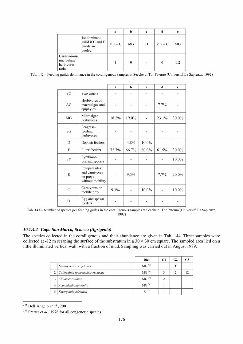
176

a b c d e

1st dominant guild if C and E guilds are pooled

MG – C MG D MG – E MG

Carnivorous/ microalgae herbivores ratio

1 0 - 0 0.2

Tab. 142 – Feeding guilds dominance in the coralligenous samples at Secche di Tor Paterno (Università La Sapienza, 1992)

a b c d e

SC Scavengers - - - - -

AG Herbivores of macroalgae and epiphytes

- - - 7.7% -

MG Microalgae herbivores 18.2% 19.0% - 23.1% 30.0%

SG Seagrass-feeding herbivores

- - - - -

D Deposit feeders - 4.8% 10.0% - -

F Filter feeders 72.7% 66.7% 80.0% 61.5% 30.0%

SY Symbiont-bearing species - - - - 10.0%

E

Ectoparasites and carnivores on preys without mobility

- 9.5% - 7.7% 20.0%

C Carnivores on mobile prey 9.1% - 10.0% - 10.0%

O Egg and spawn feeders - - - - -

Tab. 143 – Number of species per feeding guilds in the coralligenous samples at Secche di Tor Paterno (Università La Sapienza, 1992)

10.1.4.2 Capo San Marco, Sciacca (Agrigento) The species collected in the coralligenous and their abundance are given in Tab. 144. Three samples were collected at -12 m scraping the surface of the substratum in a 30 × 30 cm square. The sampled area lied on a little illuminated vertical wall, with a fraction of mud. Sampling was carried out in August 1989.

Diet G1 G2 G3

1 Lepidopleurus cajetanus MG 345 1

2 Callochiton septemvalvis euplaeae MG 345 3 2 12

3 Chiton corallinus MG 345 2

4 Acanthichitona crinita MG 345 1

5 Emarginula adriatica E 346 1

345 Dell’Angelo et al., 2001 346 Fretter et al., 1976 for all congeneric species

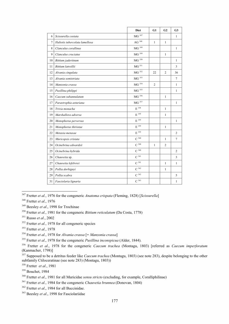
177

Diet G1 G2 G3

6 Scissurella costata MG 347 1

7 Haliotis tubercolata lamellosa AG 348 1 1

8 Clanculus corallinus MG 349 1

9 Clanculus cruciatus MG 349 1

10 Bittium jadertinum MG 350 1

11 Bittium latreillii MG 351 3

12 Alvania cingulata MG 352 22 2 36

13 Alvania semistriata MG 353 7

14 Manzonia crassa MG 354 2 1

15 Pusillina philippi MG 355 1

16 Caecum subannulatum MG 356 1

17 Parastrophia asturiana MG 357 1

18 Trivia monacha E 358 1

19 Marshallora adversa E 359 1

20 Monophorus perversus E 359 1

21 Monophorus thiriotae E 359 1

22 Metaxia metaxae E 359 2

23 Muricopsis cristata C 360 1 7

24 Ocinebrina edwardsii C 360 1 2

25 Ocinebrina hybrida C 360 2

26 Chauvetia sp. C 361 3

27 Chauvetia lefebvrei C 361 1 1

28 Pollia dorbignyi C 362 1

29 Pollia scabra C 362 5

31 Fasciolaria lignaria C 363 1

347 Fretter et al., 1976 for the congeneric Anatoma crispata (Fleming, 1828) [Scissurella] 348 Fretter et al., 1976 349 Beesley et al., 1998 for Trochinae 350 Fretter et al., 1981 for the congeneric Bittium reticulatum (Da Costa, 1778) 351 Russo et al., 2002 352 Fretter et al., 1978 for all congeneric species 353 Fretter et al., 1978 354 Fretter et al., 1978 for Alvania crassa [= Manzonia crassa] 355 Fretter et al., 1978 for the congeneric Pusillina inconspicua (Alder, 1844). 356 Fretter et al., 1978 for the congeneric Caecum trachea (Montagu, 1803) [referred as Caecum imperforatum (Kanmacher, 1798)] 357 Supposed to be a detritus feeder like Caecum trachea (Montagu, 1803) (see note 283), despite belonging to the other subfamily Ctiloceratinae (see note 283) (Montagu, 1803)) 358 Fretter et al., 1981 359 Bouchet, 1984 360 Fretter et al., 1981 for all Muricidae sensu stricto (excluding, for example, Coralliphilinae) 361 Fretter et al., 1984 for the congeneric Chauvetia brunnea (Donovan, 1804) 362 Fretter et al., 1984 for all Buccinidae. 363 Beesley et al., 1998 for Fasciolariidae

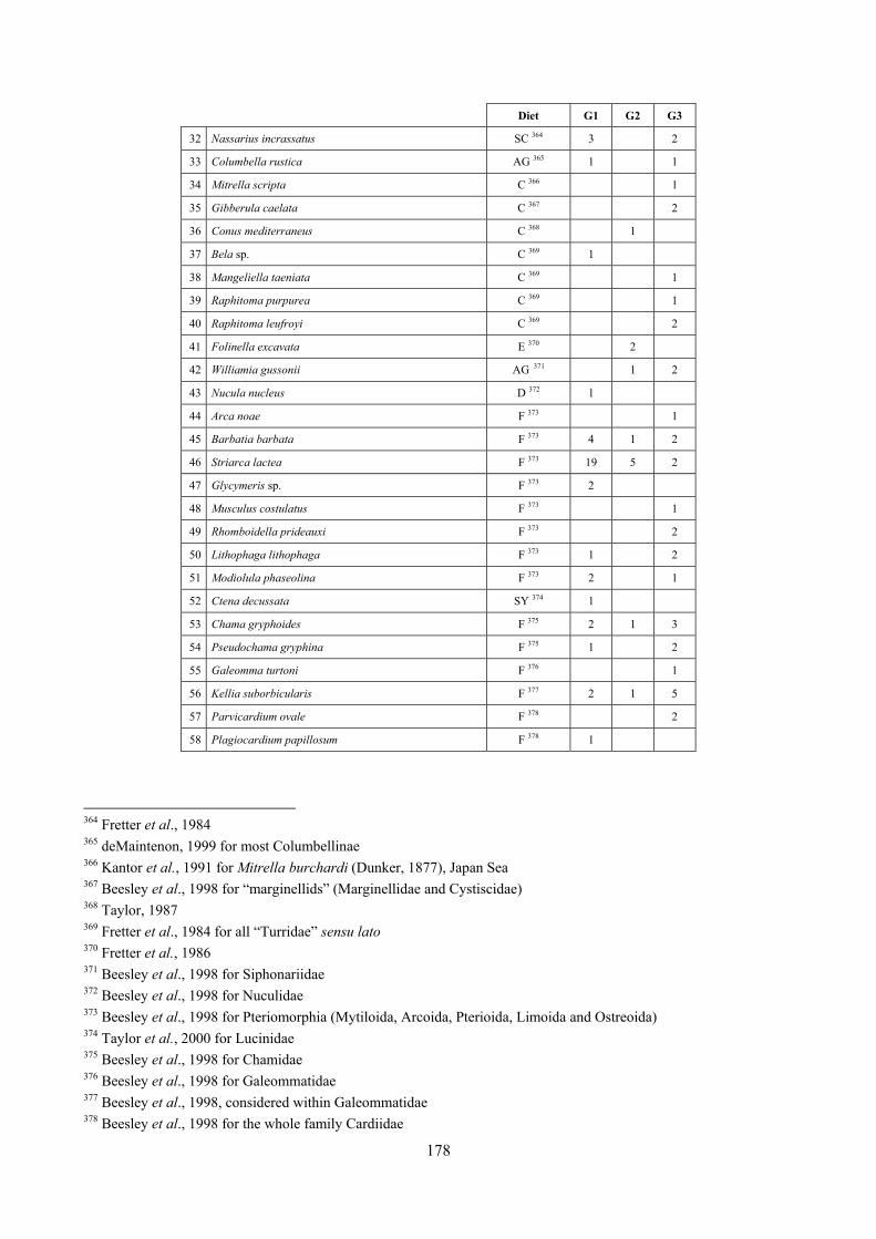
178

Diet G1 G2 G3

32 Nassarius incrassatus SC 364 3 2

33 Columbella rustica AG 365 1 1

34 Mitrella scripta C 366 1

35 Gibberula caelata C 367 2

36 Conus mediterraneus C 368 1

37 Bela sp. C 369 1

38 Mangeliella taeniata C 369 1

39 Raphitoma purpurea C 369 1

40 Raphitoma leufroyi C 369 2

41 Folinella excavata E 370 2

42 Williamia gussonii AG 371 1 2

43 Nucula nucleus D 372 1

44 Arca noae F 373 1

45 Barbatia barbata F 373 4 1 2

46 Striarca lactea F 373 19 5 2

47 Glycymeris sp. F 373 2

48 Musculus costulatus F 373 1

49 Rhomboidella prideauxi F 373 2

50 Lithophaga lithophaga F 373 1 2

51 Modiolula phaseolina F 373 2 1

52 Ctena decussata SY 374 1

53 Chama gryphoides F 375 2 1 3

54 Pseudochama gryphina F 375 1 2

55 Galeomma turtoni F 376 1

56 Kellia suborbicularis F 377 2 1 5

57 Parvicardium ovale F 378 2

58 Plagiocardium papillosum F 378 1

364 Fretter et al., 1984 365 deMaintenon, 1999 for most Columbellinae 366 Kantor et al., 1991 for Mitrella burchardi (Dunker, 1877), Japan Sea 367 Beesley et al., 1998 for “marginellids” (Marginellidae and Cystiscidae) 368 Taylor, 1987 369 Fretter et al., 1984 for all “Turridae” sensu lato 370 Fretter et al., 1986 371 Beesley et al., 1998 for Siphonariidae 372 Beesley et al., 1998 for Nuculidae 373 Beesley et al., 1998 for Pteriomorphia (Mytiloida, Arcoida, Pterioida, Limoida and Ostreoida) 374 Taylor et al., 2000 for Lucinidae 375 Beesley et al., 1998 for Chamidae 376 Beesley et al., 1998 for Galeommatidae 377 Beesley et al., 1998, considered within Galeommatidae 378 Beesley et al., 1998 for the whole family Cardiidae

179

Diet G1 G2 G3

59 Abra alba D 379 2 4

60 Chamelea gallina F 380 1

61 Gastrochaena dubia F 381 3

62 Hiatella rugosa F 382 8 3 24

TOTAL NUMBER OF SPECIMENS 87 32 150

Tab. 144 – Quali-quantitative data of the coralligenous samples, Capo San Marco, Sciacca (Agrigento)

By a population structure point of view, species richness along replicates ranges from 22 to 40. Shannon diversity index ranges from 2.561 to 2.941 and evenness from 0.796 to 0.951 (Tab. 145).

Replicate S H' J'

G1 25 2.561 0.796

G2 22 2.938 0.951

G3 40 2.941 0.797

Tab. 145 – Biodiversity indices values for coralligenous samples at Sciacca (Agrigento)

Diversity and equitability indices are influenced by dominance phenomena (Tab. 146, Tab. 147). Remarkably, Alvania cingulata is the dominant species in samples G1 (25.3%) and G3 (24%), Striarca lactea is dominant in G2 (15.6%) and the second most abundant species in G1 (21.8%) while Hiatella rugosa is the second dominant species in G2 (9.4%) and G3 (16%). Bittium latreillii which is usually a very common species is absent (G1 and G2) or present in very limited numbers (G3, only 3 specimens, 2%). Striarca lactea and Hiatella rugosa are bivalves which settle on hard substratum with their byssum. Truly infaunal species of soft substratum which exploit the sediment pools in the coralligenous are very limited in number in these samples.

Diet G1 G2 G3

1 Lepidopleurus cajetanus MG - 3.1% -

2 Callochiton septemvalvis euplaeae MG 3.4% 6.3% 8.0%

3 Chiton corallinus MG 2.3% - -

4 Acanthichitona crinita MG 1.1% - -

5 Emarginula adriatica E 1.1% - -

6 Scissurella costata MG - - 0.7%

7 Haliotis tubercolata lamellosa AG 1.1% 3.1% -

8 Clanculus corallinus MG - - 0.7%

9 Clanculus cruciatus MG - 3.1% -

10 Bittium jadertinum MG - - 0.7%

11 Bittium latreillii MG - - 2.0%

12 Alvania cingulata MG 25.3% 6.3% 24.0%

13 Alvania semistriata MG - - 4.7%

379 Hughes, 1973 for Abra tenuis (Montagu, 1803) 380 Beesley et al., 1998 for the whole family Veneridae 381 Beesley et al., 1998 for the whole family Gastrochaenidae 382 Gofas, 2009b

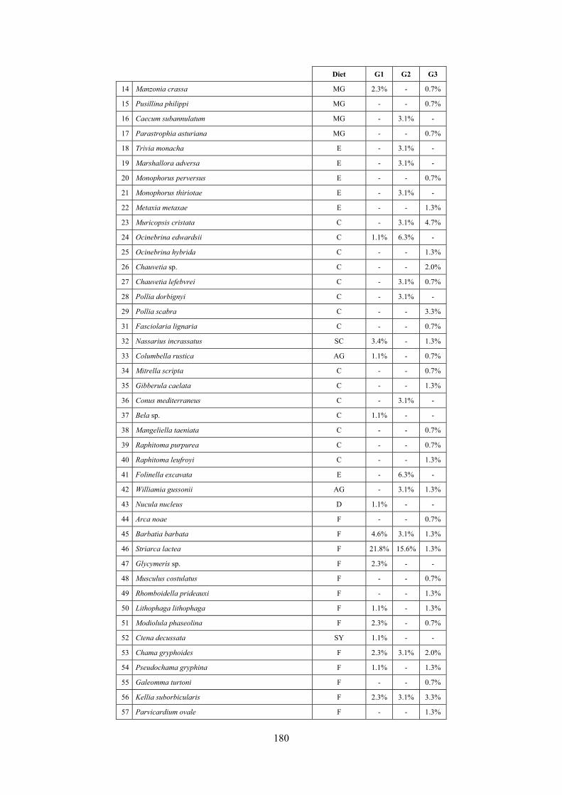
180

Diet G1 G2 G3

14 Manzonia crassa MG 2.3% - 0.7%

15 Pusillina philippi MG - - 0.7%

16 Caecum subannulatum MG - 3.1% -

17 Parastrophia asturiana MG - - 0.7%

18 Trivia monacha E - 3.1% -

19 Marshallora adversa E - 3.1% -

20 Monophorus perversus E - - 0.7%

21 Monophorus thiriotae E - 3.1% -

22 Metaxia metaxae E - - 1.3%

23 Muricopsis cristata C - 3.1% 4.7%

24 Ocinebrina edwardsii C 1.1% 6.3% -

25 Ocinebrina hybrida C - - 1.3%

26 Chauvetia sp. C - - 2.0%

27 Chauvetia lefebvrei C - 3.1% 0.7%

28 Pollia dorbignyi C - 3.1% -

29 Pollia scabra C - - 3.3%

31 Fasciolaria lignaria C - - 0.7%

32 Nassarius incrassatus SC 3.4% - 1.3%

33 Columbella rustica AG 1.1% - 0.7%

34 Mitrella scripta C - - 0.7%

35 Gibberula caelata C - - 1.3%

36 Conus mediterraneus C - 3.1% -

37 Bela sp. C 1.1% - -

38 Mangeliella taeniata C - - 0.7%

39 Raphitoma purpurea C - - 0.7%

40 Raphitoma leufroyi C - - 1.3%

41 Folinella excavata E - 6.3% -

42 Williamia gussonii AG - 3.1% 1.3%

43 Nucula nucleus D 1.1% - -

44 Arca noae F - - 0.7%

45 Barbatia barbata F 4.6% 3.1% 1.3%

46 Striarca lactea F 21.8% 15.6% 1.3%

47 Glycymeris sp. F 2.3% - -

48 Musculus costulatus F - - 0.7%

49 Rhomboidella prideauxi F - - 1.3%

50 Lithophaga lithophaga F 1.1% - 1.3%

51 Modiolula phaseolina F 2.3% - 0.7%

52 Ctena decussata SY 1.1% - -

53 Chama gryphoides F 2.3% 3.1% 2.0%

54 Pseudochama gryphina F 1.1% - 1.3%

55 Galeomma turtoni F - - 0.7%

56 Kellia suborbicularis F 2.3% 3.1% 3.3%

57 Parvicardium ovale F - - 1.3%

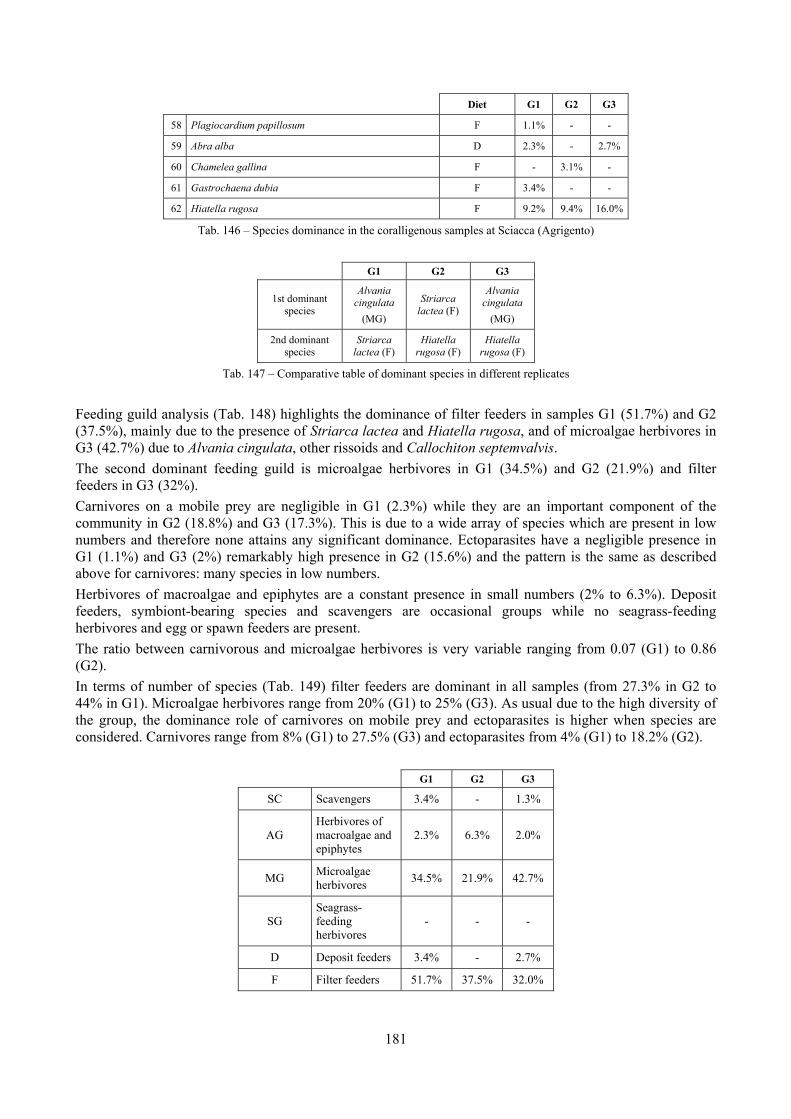
181

Diet G1 G2 G3

58 Plagiocardium papillosum F 1.1% - -

59 Abra alba D 2.3% - 2.7%

60 Chamelea gallina F - 3.1% -

61 Gastrochaena dubia F 3.4% - -

62 Hiatella rugosa F 9.2% 9.4% 16.0%

Tab. 146 – Species dominance in the coralligenous samples at Sciacca (Agrigento)

G1 G2 G3

1st dominant species

Alvania cingulata

(MG)

Striarca lactea (F)

Alvania cingulata

(MG)

2nd dominant species

Striarca lactea (F)

Hiatella rugosa (F)

Hiatella rugosa (F)

Tab. 147 – Comparative table of dominant species in different replicates

Feeding guild analysis (Tab. 148) highlights the dominance of filter feeders in samples G1 (51.7%) and G2 (37.5%), mainly due to the presence of Striarca lactea and Hiatella rugosa, and of microalgae herbivores in G3 (42.7%) due to Alvania cingulata, other rissoids and Callochiton septemvalvis. The second dominant feeding guild is microalgae herbivores in G1 (34.5%) and G2 (21.9%) and filter feeders in G3 (32%). Carnivores on a mobile prey are negligible in G1 (2.3%) while they are an important component of the community in G2 (18.8%) and G3 (17.3%). This is due to a wide array of species which are present in low numbers and therefore none attains any significant dominance. Ectoparasites have a negligible presence in G1 (1.1%) and G3 (2%) remarkably high presence in G2 (15.6%) and the pattern is the same as described above for carnivores: many species in low numbers. Herbivores of macroalgae and epiphytes are a constant presence in small numbers (2% to 6.3%). Deposit feeders, symbiont-bearing species and scavengers are occasional groups while no seagrass-feeding herbivores and egg or spawn feeders are present. The ratio between carnivorous and microalgae herbivores is very variable ranging from 0.07 (G1) to 0.86 (G2). In terms of number of species (Tab. 149) filter feeders are dominant in all samples (from 27.3% in G2 to 44% in G1). Microalgae herbivores range from 20% (G1) to 25% (G3). As usual due to the high diversity of the group, the dominance role of carnivores on mobile prey and ectoparasites is higher when species are considered. Carnivores range from 8% (G1) to 27.5% (G3) and ectoparasites from 4% (G1) to 18.2% (G2).

G1 G2 G3

SC Scavengers 3.4% - 1.3%

AG Herbivores of macroalgae and epiphytes

2.3% 6.3% 2.0%

MG Microalgae herbivores 34.5% 21.9% 42.7%

SG Seagrass-feeding herbivores

- - -

D Deposit feeders 3.4% - 2.7%

F Filter feeders 51.7% 37.5% 32.0%

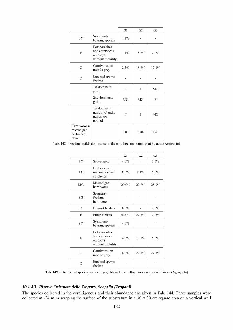
182

G1 G2 G3

SY Symbiont-bearing species 1.1% - -

E

Ectoparasites and carnivores on preys without mobility

1.1% 15.6% 2.0%

C Carnivores on mobile prey 2.3% 18.8% 17.3%

O Egg and spawn feeders - - -

1st dominant guild F F MG

2nd dominant guild MG MG F

1st dominant guild if C and E guilds are pooled

F F MG

Carnivorous/ microalgae herbivores ratio

0.07 0.86 0.41

Tab. 148 – Feeding guilds dominance in the coralligenous samples at Sciacca (Agrigento)

G1 G2 G3

SC Scavengers 4.0% - 2.5%

AG Herbivores of macroalgae and epiphytes

8.0% 9.1% 5.0%

MG Microalgae herbivores 20.0% 22.7% 25.0%

SG Seagrass-feeding herbivores

- - -

D Deposit feeders 8.0% - 2.5%

F Filter feeders 44.0% 27.3% 32.5%

SY Symbiont-bearing species 4.0% - -

E

Ectoparasites and carnivores on preys without mobility

4.0% 18.2% 5.0%

C Carnivores on mobile prey 8.0% 22.7% 27.5%

O Egg and spawn feeders - - -

Tab. 149 – Number of species per feeding guilds in the coralligenous samples at Sciacca (Agrigento)

10.1.4.3 Riserva Orientata dello Zingaro, Scopello (Trapani) The species collected in the coralligenous and their abundance are given in Tab. 144. Three samples were collected at -24 m m scraping the surface of the substratum in a 30 × 30 cm square area on a vertical wall

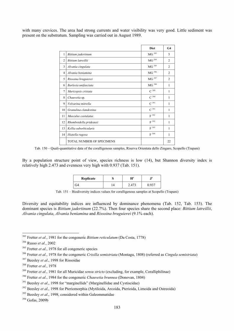
183

with many crevices. The area had strong currents and water visibility was very good. Little sediment was present on the substratum. Sampling was carried out in August 1989.

Diet G4

1 Bittium jadertinum MG 383 5

2 Bittium latreillii MG 384 2

3 Alvania cingulata MG 385 2

4 Alvania beniamina MG 386 2

5 Rissoina bruguierei MG 387 2

6 Barleeia unifasciata MG 388 1

7 Muricopsis cristata C 389 1

8 Chauvetia sp. C 390 1

9 Volvarina mitrella C 391 1

10 Granulina clandestina C 391 1

11 Musculus costulatus F 392 1

12 Rhomboidella prideauxi F 392 1

13 Kellia suborbicularis F 393 1

14 Hiatella rugosa F 394 1

TOTAL NUMBER OF SPECIMENS 22

Tab. 150 – Quali-quantitative data of the coralligenous samples, Riserva Orientata dello Zingaro, Scopello (Trapani)

By a population structure point of view, species richness is low (14), but Shannon diversity index is relatively high 2.473 and evenness very high with 0.937 (Tab. 151).

Replicate S H' J'

G4 14 2.473 0.937

Tab. 151 – Biodiversity indices values for coralligenous samples at Scopello (Trapani)

Diversity and equitability indices are influenced by dominance phenomena (Tab. 152, Tab. 153). The dominant species is Bittium jadertinum (22.7%). Then four species share the second place: Bittium latreillii, Alvania cingulata, Alvania beniamina and Rissoina bruguierei (9.1% each).

383 Fretter et al., 1981 for the congeneric Bittium reticulatum (Da Costa, 1778) 384 Russo et al., 2002 385 Fretter et al., 1978 for all congeneric species 386 Fretter et al., 1978 for the congeneric Crisilla semistriata (Montagu, 1808) (referred as Cingula semistriata) 387 Beesley et al., 1998 for Rissoidae 388 Fretter et al., 1978 389 Fretter et al., 1981 for all Muricidae sensu stricto (excluding, for example, Coralliphilinae) 390 Fretter et al., 1984 for the congeneric Chauvetia brunnea (Donovan, 1804) 391 Beesley et al., 1998 for “marginellids” (Marginellidae and Cystiscidae) 392 Beesley et al., 1998 for Pteriomorphia (Mytiloida, Arcoida, Pterioida, Limoida and Ostreoida) 393 Beesley et al., 1998, considered within Galeommatidae 394 Gofas, 2009b

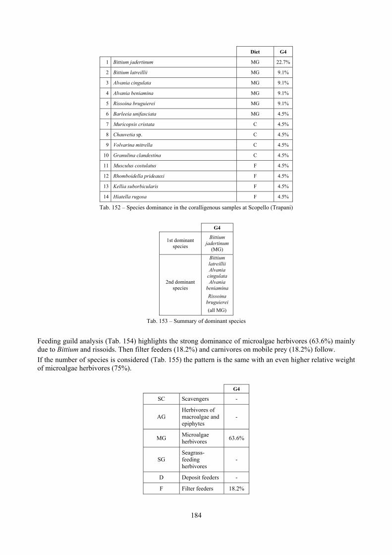
184

Diet G4

1 Bittium jadertinum MG 22.7%

2 Bittium latreillii MG 9.1%

3 Alvania cingulata MG 9.1%

4 Alvania beniamina MG 9.1%

5 Rissoina bruguierei MG 9.1%

6 Barleeia unifasciata MG 4.5%

7 Muricopsis cristata C 4.5%

8 Chauvetia sp. C 4.5%

9 Volvarina mitrella C 4.5%

10 Granulina clandestina C 4.5%

11 Musculus costulatus F 4.5%

12 Rhomboidella prideauxi F 4.5%

13 Kellia suborbicularis F 4.5%

14 Hiatella rugosa F 4.5%

Tab. 152 – Species dominance in the coralligenous samples at Scopello (Trapani)

G4

1st dominant species

Bittium jadertinum

(MG)

2nd dominant species

Bittium latreillii Alvania

cingulata Alvania

beniamina Rissoina

bruguierei (all MG)

Tab. 153 – Summary of dominant species

Feeding guild analysis (Tab. 154) highlights the strong dominance of microalgae herbivores (63.6%) mainly due to Bittium and rissoids. Then filter feeders (18.2%) and carnivores on mobile prey (18.2%) follow. If the number of species is considered (Tab. 155) the pattern is the same with an even higher relative weight of microalgae herbivores (75%).

G4

SC Scavengers -

AG Herbivores of macroalgae and epiphytes

-

MG Microalgae herbivores 63.6%

SG Seagrass-feeding herbivores

-

D Deposit feeders -

F Filter feeders 18.2%

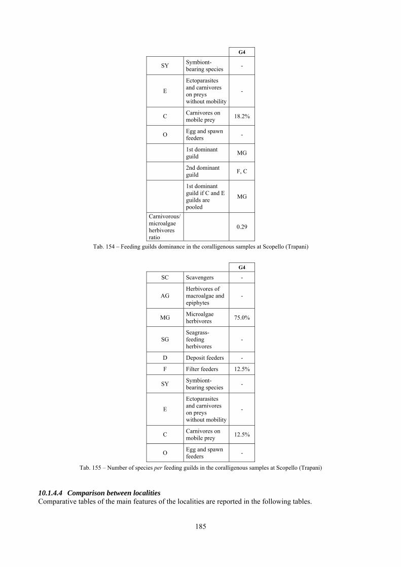
185

G4

SY Symbiont-bearing species -

E

Ectoparasites and carnivores on preys without mobility

-

C Carnivores on mobile prey 18.2%

O Egg and spawn feeders -

1st dominant guild MG

2nd dominant guild F, C

1st dominant guild if C and E guilds are pooled

MG

Carnivorous/ microalgae herbivores ratio

0.29

Tab. 154 – Feeding guilds dominance in the coralligenous samples at Scopello (Trapani)

G4

SC Scavengers -

AG Herbivores of macroalgae and epiphytes

-

MG Microalgae herbivores 75.0%

SG Seagrass-feeding herbivores

-

D Deposit feeders -

F Filter feeders 12.5%

SY Symbiont-bearing species -

E

Ectoparasites and carnivores on preys without mobility

-

C Carnivores on mobile prey 12.5%

O Egg and spawn feeders -

Tab. 155 – Number of species per feeding guilds in the coralligenous samples at Scopello (Trapani)

10.1.4.4 Comparison between localities Comparative tables of the main features of the localities are reported in the following tables.

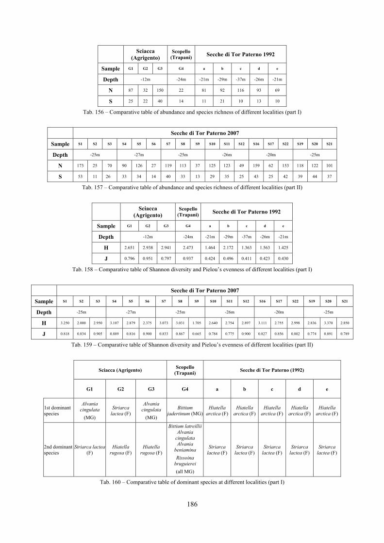
186

Sciacca (Agrigento)

Scopello (Trapani) Secche di Tor Paterno 1992

Sample G1 G2 G3 G4 a b c d e

Depth -12m -24m -21m -29m -37m -26m -21m

N 87 32 150 22 81 92 116 93 69

S 25 22 40 14 11 21 10 13 10

Tab. 156 – Comparative table of abundance and species richness of different localities (part I)

Secche di Tor Paterno 2007

Sample S1 S2 S3 S4 S5 S6 S7 S8 S9 S10 S11 S12 S16 S17 S22 S19 S20 S21

Depth -25m -27m -25m -26m -20m -25m

N 173 25 70 90 126 27 119 113 37 125 123 49 159 62 153 118 122 101

S 53 11 26 33 34 14 40 33 13 29 35 25 43 25 42 39 44 37

Tab. 157 – Comparative table of abundance and species richness of different localities (part II)

Sciacca (Agrigento)

Scopello (Trapani) Secche di Tor Paterno 1992

Sample G1 G2 G3 G4 a b c d e

Depth -12m -24m -21m -29m -37m -26m -21m

H 2.651 2.938 2.941 2.473 1.464 2.172 1.363 1.563 1.425

J 0.796 0.951 0.797 0.937 0.424 0.496 0.411 0.423 0.430

Tab. 158 – Comparative table of Shannon diversity and Pielou’s evenness of different localities (part I)

Secche di Tor Paterno 2007

Sample S1 S2 S3 S4 S5 S6 S7 S8 S9 S10 S11 S12 S16 S17 S22 S19 S20 S21

Depth -25m -27m -25m -26m -20m -25m

H 3.250 2.000 2.950 3.107 2.879 2.375 3.073 3.031 1.705 2.640 2.754 2.897 3.111 2.755 2.998 2.836 3.370 2.850

J 0.818 0.834 0.905 0.889 0.816 0.900 0.833 0.867 0.665 0.784 0.775 0.900 0.827 0.856 0.802 0.774 0.891 0.789

Tab. 159 – Comparative table of Shannon diversity and Pielou’s evenness of different localities (part II)

Sciacca (Agrigento) Scopello

(Trapani) Secche di Tor Paterno (1992)

G1 G2 G3 G4 a b c d e

1st dominant species

Alvania cingulata

(MG)

Striarca lactea (F)

Alvania cingulata

(MG)

Bittium jadertinum (MG)

Hiatella arctica (F)

Hiatella arctica (F)

Hiatella arctica (F)

Hiatella arctica (F)

Hiatella arctica (F)

2nd dominant species

Striarca lactea (F)

Hiatella rugosa (F)

Hiatella rugosa (F)

Bittium latreilliiAlvania

cingulata Alvania

beniamina Rissoina

bruguierei (all MG)

Striarca lactea (F)

Striarca lactea (F)

Striarca lactea (F)

Striarca lactea (F)

Striarca lactea (F)

Tab. 160 – Comparative table of dominant species at different localities (part I)

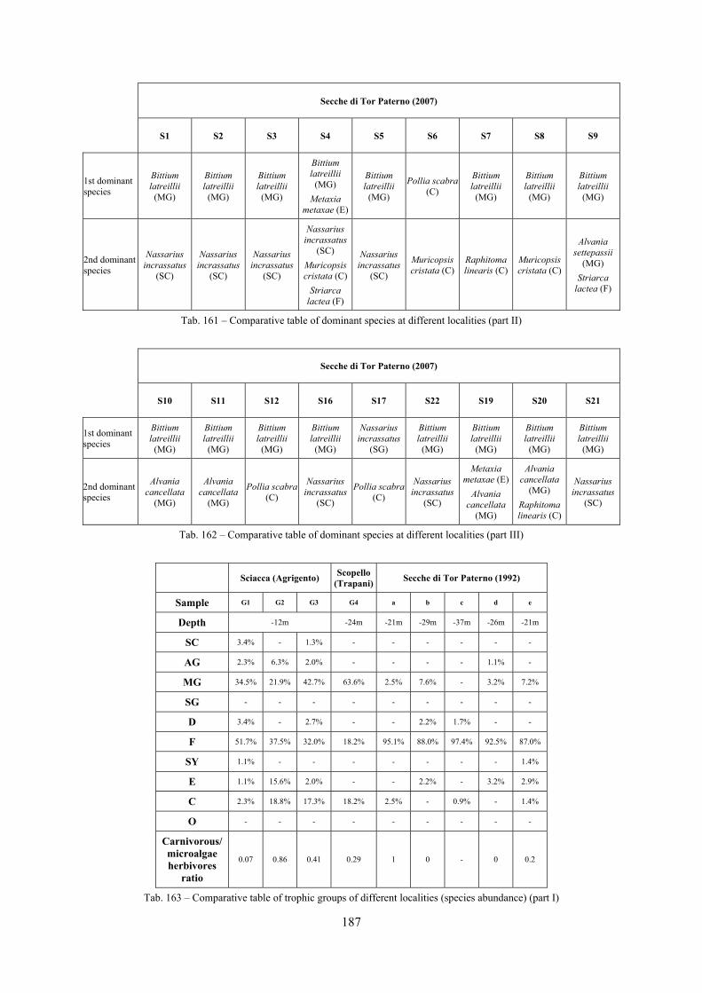
187

Secche di Tor Paterno (2007)

S1 S2 S3 S4 S5 S6 S7 S8 S9

1st dominant species

Bittium latreillii

(MG)

Bittium latreillii

(MG)

Bittium latreillii

(MG)

Bittium latreillii

(MG) Metaxia

metaxae (E)

Bittium latreillii

(MG)

Pollia scabra (C)

Bittium latreillii

(MG)

Bittium latreillii

(MG)

Bittium latreillii

(MG)

2nd dominant species

Nassarius incrassatus

(SC)

Nassarius incrassatus

(SC)

Nassarius incrassatus

(SC)

Nassarius incrassatus

(SC) Muricopsis cristata (C)

Striarca lactea (F)

Nassarius incrassatus

(SC)

Muricopsis cristata (C)

Raphitoma linearis (C)

Muricopsis cristata (C)

Alvania settepassii

(MG) Striarca

lactea (F)

Tab. 161 – Comparative table of dominant species at different localities (part II)

Secche di Tor Paterno (2007)

S10 S11 S12 S16 S17 S22 S19 S20 S21

1st dominant species

Bittium latreillii

(MG)

Bittium latreillii

(MG)

Bittium latreillii

(MG)

Bittium latreillii

(MG)

Nassarius incrassatus

(SG)

Bittium latreillii

(MG)

Bittium latreillii

(MG)

Bittium latreillii

(MG)

Bittium latreillii

(MG)

2nd dominant species

Alvania cancellata

(MG)

Alvania cancellata

(MG)

Pollia scabra(C)

Nassarius incrassatus

(SC)

Pollia scabra(C)

Nassarius incrassatus

(SC)

Metaxia metaxae (E)

Alvania cancellata

(MG)

Alvania cancellata

(MG) Raphitoma linearis (C)

Nassarius incrassatus

(SC)

Tab. 162 – Comparative table of dominant species at different localities (part III)

Sciacca (Agrigento) Scopello (Trapani) Secche di Tor Paterno (1992)

Sample G1 G2 G3 G4 a b c d e

Depth -12m -24m -21m -29m -37m -26m -21m

SC 3.4% - 1.3% - - - - - -

AG 2.3% 6.3% 2.0% - - - - 1.1% -

MG 34.5% 21.9% 42.7% 63.6% 2.5% 7.6% - 3.2% 7.2%

SG - - - - - - - - -

D 3.4% - 2.7% - - 2.2% 1.7% - -

F 51.7% 37.5% 32.0% 18.2% 95.1% 88.0% 97.4% 92.5% 87.0%

SY 1.1% - - - - - - - 1.4%

E 1.1% 15.6% 2.0% - - 2.2% - 3.2% 2.9%

C 2.3% 18.8% 17.3% 18.2% 2.5% - 0.9% - 1.4%

O - - - - - - - - -

Carnivorous/ microalgae herbivores

ratio

0.07 0.86 0.41 0.29 1 0 - 0 0.2

Tab. 163 – Comparative table of trophic groups of different localities (species abundance) (part I)

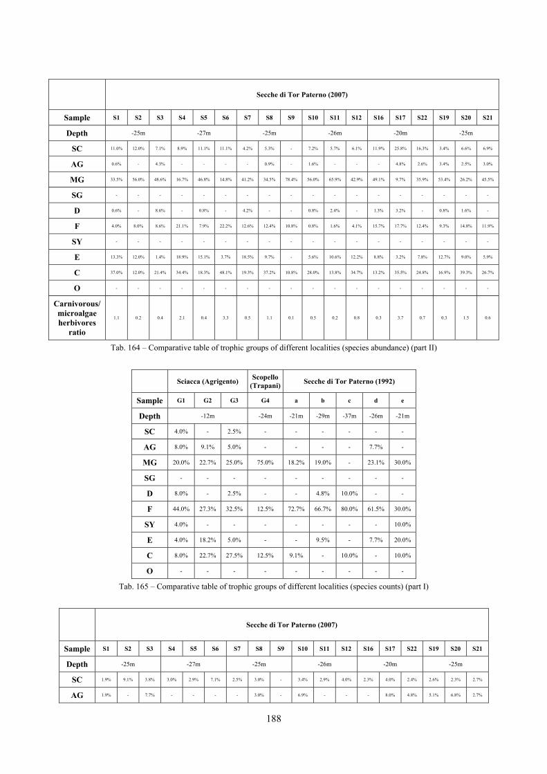
188

Secche di Tor Paterno (2007)

Sample S1 S2 S3 S4 S5 S6 S7 S8 S9 S10 S11 S12 S16 S17 S22 S19 S20 S21

Depth -25m -27m -25m -26m -20m -25m

SC 11.0% 12.0% 7.1% 8.9% 11.1% 11.1% 4.2% 5.3% - 7.2% 5.7% 6.1% 11.9% 25.8% 16.3% 3.4% 6.6% 6.9%

AG 0.6% - 4.3% - - - - 0.9% - 1.6% - - - 4.8% 2.6% 3.4% 2.5% 3.0%

MG 33.5% 56.0% 48.6% 16.7% 46.8% 14.8% 41.2% 34.5% 78.4% 56.0% 65.9% 42.9% 49.1% 9.7% 35.9% 53.4% 26.2% 45.5%

SG - - - - - - - - - - - - - - - - - -

D 0.6% - 8.6% - 0.8% - 4.2% - - 0.8% 2.4% - 1.3% 3.2% - 0.8% 1.6% -

F 4.0% 8.0% 8.6% 21.1% 7.9% 22.2% 12.6% 12.4% 10.8% 0.8% 1.6% 4.1% 15.7% 17.7% 12.4% 9.3% 14.8% 11.9%

SY - - - - - - - - - - - - - - - - - -

E 13.3% 12.0% 1.4% 18.9% 15.1% 3.7% 18.5% 9.7% - 5.6% 10.6% 12.2% 8.8% 3.2% 7.8% 12.7% 9.0% 5.9%

C 37.0% 12.0% 21.4% 34.4% 18.3% 48.1% 19.3% 37.2% 10.8% 28.0% 13.8% 34.7% 13.2% 35.5% 24.8% 16.9% 39.3% 26.7%

O - - - - - - - - - - - - - - - - - -

Carnivorous/ microalgae herbivores

ratio

1.1 0.2 0.4 2.1 0.4 3.3 0.5 1.1 0.1 0.5 0.2 0.8 0.3 3.7 0.7 0.3 1.5 0.6

Tab. 164 – Comparative table of trophic groups of different localities (species abundance) (part II)

Sciacca (Agrigento) Scopello (Trapani) Secche di Tor Paterno (1992)

Sample G1 G2 G3 G4 a b c d e

Depth -12m -24m -21m -29m -37m -26m -21m

SC 4.0% - 2.5% - - - - - -

AG 8.0% 9.1% 5.0% - - - - 7.7% -

MG 20.0% 22.7% 25.0% 75.0% 18.2% 19.0% - 23.1% 30.0%

SG - - - - - - - - -

D 8.0% - 2.5% - - 4.8% 10.0% - -

F 44.0% 27.3% 32.5% 12.5% 72.7% 66.7% 80.0% 61.5% 30.0%

SY 4.0% - - - - - - - 10.0%

E 4.0% 18.2% 5.0% - - 9.5% - 7.7% 20.0%

C 8.0% 22.7% 27.5% 12.5% 9.1% - 10.0% - 10.0%

O - - - - - - - - -

Tab. 165 – Comparative table of trophic groups of different localities (species counts) (part I)

Secche di Tor Paterno (2007)

Sample S1 S2 S3 S4 S5 S6 S7 S8 S9 S10 S11 S12 S16 S17 S22 S19 S20 S21

Depth -25m -27m -25m -26m -20m -25m

SC 1.9% 9.1% 3.8% 3.0% 2.9% 7.1% 2.5% 3.0% - 3.4% 2.9% 4.0% 2.3% 4.0% 2.4% 2.6% 2.3% 2.7%

AG 1.9% - 7.7% - - - - 3.0% - 6.9% - - - 8.0% 4.8% 5.1% 6.8% 2.7%

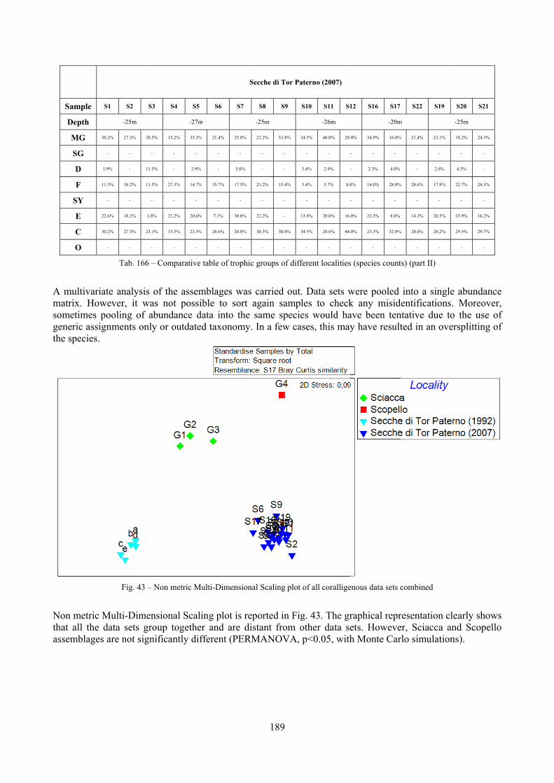
Sample

Depth

MG

SG

D

F

SY

E

C

O

A multivarimatrix. Howsometimes generic assithe species.

Non metric that all the assemblage

S1 S2 S

-25m

30.2% 27.3% 38

- -

1.9% - 11

11.3% 18.2% 11

- -

22.6% 18.2% 3.

30.2% 27.3% 23

- -

Tab. 166

iate analysis wever, it wapooling of aignments onl

Fig. 43 –

Multi-Dimedata sets gr

s are not sign

S3 S4 S5

-27m

.5% 15.2% 35.3%

- - -

.5% - 2.9%

.5% 27.3% 14.7%

- - -

8% 21.2% 20.6%

.1% 33.3% 23.5%

- - -

– Comparative

of the assemas not possiabundance dly or outdate

– Non metric M

ensional Scalroup togethenificantly dif

S

S6 S7

m

% 21.4% 25.0%

- -

% - 5.0%

% 35.7% 17.5%

- -

% 7.1% 30.0%

% 28.6% 20.0%

- -

e table of trophi

mblages wasible to sort

data into the ed taxonomy

Multi-Dimension

ling plot is reer and are different (PER

189

Secche di Tor Pa

S8 S9

-25m

21.2% 53.8%

- -

- -

21.2% 15.4%

- -

21.2% -

30.3% 30.8%

- -

c groups of diff

s carried outagain sampsame specie

. In a few ca

nal Scaling plot

eported in Figistant from o

RMANOVA,

aterno (2007)

S10 S11 S1

-26m

34.5% 40.0% 28.

- - -

3.4% 2.9% -

3.4% 5.7% 8.0

- - -

13.8% 20.0% 16.

34.5% 28.6% 44.

- - -

ferent localities

. Data sets wles to checkes would ha

ases, this may

of all corallige

g. 43. The grother data sep<0.05, with

12 S16 S17

-20m

0% 34.9% 16.0%

- - -

- 2.3% 4.0%

0% 14.0% 28.0%

- - -

0% 23.3% 8.0%

0% 23.3% 32.0%

- - -

s (species count

were pooled k any misidave been teny have result

enous data sets c

raphical reprets. Howeveh Monte Car

S22 S19

m

% 21.4% 23.1%

- -

- 2.6%

% 28.6% 17.9%

- -

14.3% 20.5%

% 28.6% 28.2%

- -

ts) (part II)

into a singledentificationsntative due toted in an ove

combined

resentation cler, Sciacca arlo simulation

S20 S21

-25m

18.2% 24.3%

- -

4.5% -

22.7% 24.3%

- -

15.9% 16.2%

29.5% 29.7%

- -

e abundances. Moreover,o the use ofersplitting of

learly showsand Scopellons).

e , f f

s o

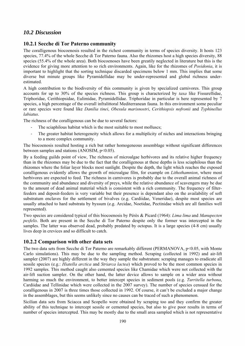
190

10.2 Discussion

10.2.1 Secche di Tor Paterno community The coralligenous biocoenosis resulted in the richest community in terms of species diversity. It hosts 123 species, 77.4% of the whole Secche di Tor Paterno fauna. Also the rhizomes host a high species diversity, 88 species (55.4% of the whole area). Both biocoenoses have been greatily neglected in literature but this is the evidence for giving more attention to so rich environments. Again, like for the rhizomes of Posidonia, it is important to highlight that the sorting technique discarded specimens below 1 mm. This implies that some diverse but minute groups like Pyramidellidae may be under-represented and global richness under-estimated. A high contribution to the biodiversity of this community is given by specialized carnivores. This group accounts for up to 30% of the species richness. This group is characterized by taxa like Fissurellidae, Triphoridae, Cerithiopsidae, Eulimidae, Pyramidellidae. Triphoridae in particular is here represented by 7 species, a high percentage of the overall infralittoral Mediterranean fauna. In this environment some peculiar or rare species were found like Danilia tinei, Obesula marisnostri, Cerithiopsis nofronii and Typhinellus labiatus. The richness of the coralligenous can be due to several factors:

‐ The sciaphilous habitat which is the most suitable to most molluscs; ‐ The greater habitat heterogeneity which allows for a multiplicity of niches and interactions bringing

to a more complex community. The biocoenosis resulted hosting a rich but rather homogeneous assemblage without significant differences between samples and stations (ANOSIM, p<0.05). By a feeding guilds point of view, The richness of microalgae herbivores and its relative higher frequency than in the rhizomes may be due to the fact that the coralligenous at these depths is less sciaphilous than the rhizomes where the foliar layer blocks most sunlight. Despite the depth, the light which reaches the exposed coralligenous evidently allows the growth of microalgae film, for example on Lithothamnion, where most herbivores are expected to feed. The richness in carnivores is probably due to the overall animal richness of the community and abundance and diversity of preys, while the relative abundance of scavengers may be due to the amount of dead animal material which is consistent with a rich community. The frequency of filter-feeders and deposit-feeders is very variable but their presence is dependant also on the availability of soft substratum enclaves for the settlement of bivalves (e.g. Cardiidae, Veneridae), despite most species are usually attached to hard substrata by byssum (e.g. Arcidae, Noetidae, Pectinidae which are all families well represented). Two species are considered typical of this biocoenosis by Pérès & Picard (1964): Lima lima and Manupecten pesfelis. Both are present in the Secche di Tor Paterno despite only the former was intercepted in the samples. The latter was observed dead, probably predated by octopus. It is a large species (4-8 cm) usually lives deep in crevices and so difficult to catch.

10.2.2 Comparison with other data sets The two data sets from Secche di Tor Paterno are remarkably different (PERMANOVA, p<0.05, with Monte Carlo simulations). This may be due to the sampling method. Scraping (collected in 1992) and air-lift sampler (2007) are highly different in the way they sample the substratum: scraping manages to eradicate all sessile species (e.g.: Hiatella arctica and Striarca lactea) which proved to be the most common species in 1992 samples. This method caught also cemented species like Chamidae which were not collected with the air-lift suction sampler. On the other hand, the latter device allows to sample on a wider area without harming so much the environment, to better intercept species in sediment pools (e.g. Turritella turbona, Cardiidae and Tellinidae which were collected in the 2007 survey). The number of species censued for the coralligenous in 2007 is three times those collected in 1992. Of course, it can’t be excluded a major change in the assemblages, but this seems unlikely since no causes can be traced of such a phenomenon. Sicilian data sets from Sciacca and Scopello were obtained by scraping too and they confirm the greater ability of this technique to intercept sessile or cemented species, but also to give poor results in terms of number of species intercepted. This may be mostly due to the small area sampled which is not representative

191

of the heterogeneity of the environment. The biodiversity evaluated by scraping is remarkably different as can be seen from the value of the Shannon index in Secche di Tor Paterno: its mean value in 1992 is just 1.597 while in 2007 it reaches 2.810! This may also evidence that despite sessile or cemented species are a part of the biodiversity in the coralligenous, the greatest share of species is vagile. In any case, the extreme dominance of Hiatella arctica and Striarca lactea in 1992 samples in Secche di Tor Paterno is remarkable and unregistered in other samples.

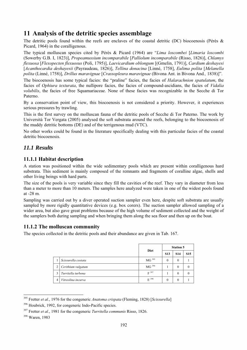
192

11 Analysis of the detritic species assemblage The detritic pools found within the reefs are enclaves of the coastal detritic (DC) biocoenosis (Pérès & Picard, 1964) in the coralligenous. The typical molluscan species cited by Pérès & Picard (1964) are “Lima loscombei [Limaria loscombi (Sowerby G.B. I, 1823)], Propeamussium incomparabile [Palliolum incomparabile (Risso, 1826)], Chlamys flexuosa [Flexopecten flexuosus (Poli, 1795)], Laevicardium oblongum [(Gmelin, 1791)], Cardium deshayesi [Acanthocardia deshayesii (Payraudeau, 1826)], Tellina donacina [Linné, 1758], Eulima polita [Melanella polita (Linné, 1758)], Drillus maravignae [Crassopleura maravignae (Bivona Ant. in Bivona And., 1838)]”. The biocoenosis has some typical facies: the “praline” facies, the facies of Halarachnion spatulatum, the facies of Ophiura texturata, the nullipore facies, the facies of compound-ascidians, the facies of Vidalia volubilis, the facies of free Squamariaceae. None of these facies was recognizable in the Secche di Tor Paterno. By a conservation point of view, this biocoenosis is not considered a priority. However, it experiences serious pressures by trawling. This is the first survey on the molluscan fauna of the detritic pools of Secche di Tor Paterno. The work by Università Tor Vergata (2005) analysed the soft substrata around the reefs, belonging to the biocoenosis of the muddy detritic bottoms (DE) and of the terrigenous mud (VTC). No other works could be found in the literature specifically dealing with this particular facies of the coastal detritic biocoenosis.

11.1 Results

11.1.1 Habitat description A station was positioned within the wide sedimentary pools which are present within coralligenous hard substrata. This sediment is mainly composed of the remnants and fragments of coralline algae, shells and other living beings with hard parts. The size of the pools is very variable since they fill the cavities of the reef. They vary in diameter from less than a meter to more than 10 meters. The samples here analyzed were taken in one of the widest pools found at -28 m. Sampling was carried out by a diver operated suction sampler even here, despite soft substrata are usually sampled by more rigidly quantitative devices (e.g. box corers). The suction sampler allowed sampling of a wider area, but also gave great problems because of the high volume of sediment collected and the weight of the samplers both during sampling and when bringing them along the sea floor and then up on the boat.

11.1.2 The molluscan community The species collected in the detritic pools and their abundance are given in Tab. 167.

Diet Station 5

S13 S14 S15

1 Scissurella costata MG 395 0 0 1

2 Cerithium vulgatum MG 396 1 0 0

3 Turritella turbona F 397 1 0 0

4 Vitreolina incurva E 398 0 0 1

395 Fretter et al., 1976 for the congeneric Anatoma crispata (Fleming, 1828) [Scissurella] 396 Houbrick, 1992, for congeneric Indo-Pacific species. 397 Fretter et al., 1981 for the congeneric Turritella communis Risso, 1826. 398 Waren, 1983

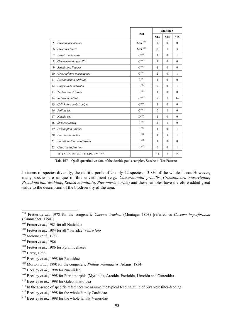
193

Diet Station 5

S13 S14 S15

5 Caecum armoricum MG 399 3 0 0

6 Caecum clarkii MG 399 0 1 3

7 Euspira pulchella C 400 1 0 1

8 Comarmondia gracilis C 401 1 0 0

9 Raphitoma linearis C 401 1 0 0

10 Crassopleura maravignae C 401 2 0 1

11 Pseudotorinia architae E 402 1 0 0

12 Chrysallida suturalis E 403 0 0 1

13 Turbonilla striatula E 404 1 0 0

14 Retusa mamillata C 405 5 1 14

15 Cylichnina crebrisculpta C 406 1 0 0

16 Philine sp. C 407 0 1 0

17 Nucula sp. D 408 1 0 0

18 Striarca lactea F 409 2 1 0

19 Hemilepton nitidum F 410 1 0 1

20 Pteromeris corbis F 411 1 3 1

21 Papillicardium papillosum F 412 1 0 0

22 Clausinella fasciata F 413 0 0 1

TOTAL NUMBER OF SPECIMENS 24 7 25

Tab. 167 – Quali-quantitative data of the detritic pools samples, Secche di Tor Paterno

In terms of species diversity, the detritic pools offer only 22 species, 13.8% of the whole fauna. However, many species are unique of this environment (e.g.: Comarmondia gracilis, Crassopleura maravignae, Pseudotorinia architae, Retusa mamillata, Pteromeris corbis) and these samples have therefore added great value to the description of the biodiversity of the area.

399 Fretter et al., 1978 for the congeneric Caecum trachea (Montagu, 1803) [referred as Caecum imperforatum (Kanmacher, 1798)] 400 Fretter et al., 1981 for all Naticidae 401 Fretter et al., 1984 for all “Turridae” sensu lato 402 Melone et al., 1982 403 Fretter et al., 1986 404 Fretter et al., 1986 for Pyramidellacea 405 Berry, 1988 406 Beesley et al., 1998 for Retusidae 407 Morton et al., 1990 for the congeneric Philine orientalis A. Adams, 1854 408 Beesley et al., 1998 for Nuculidae 409 Beesley et al., 1998 for Pteriomorphia (Mytiloida, Arcoida, Pterioida, Limoida and Ostreoida) 410 Beesley et al., 1998 for Galeommatoidea 411 In the absence of specific references we assume the typical feeding guild of bivalves: filter-feeding. 412 Beesley et al., 1998 for the whole family Cardiidae 413 Beesley et al., 1998 for the whole family Veneridae

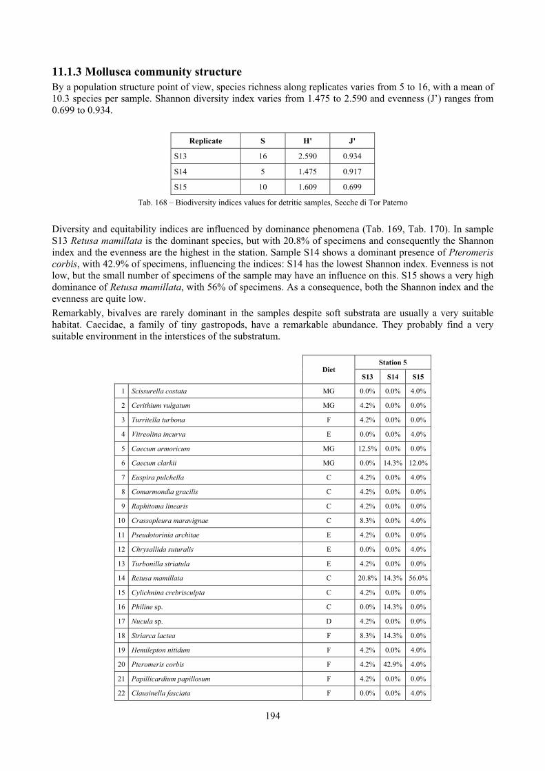
194

11.1.3 Mollusca community structure By a population structure point of view, species richness along replicates varies from 5 to 16, with a mean of 10.3 species per sample. Shannon diversity index varies from 1.475 to 2.590 and evenness (J’) ranges from 0.699 to 0.934.

Replicate S H' J'

S13 16 2.590 0.934

S14 5 1.475 0.917

S15 10 1.609 0.699

Tab. 168 – Biodiversity indices values for detritic samples, Secche di Tor Paterno

Diversity and equitability indices are influenced by dominance phenomena (Tab. 169, Tab. 170). In sample S13 Retusa mamillata is the dominant species, but with 20.8% of specimens and consequently the Shannon index and the evenness are the highest in the station. Sample S14 shows a dominant presence of Pteromeris corbis, with 42.9% of specimens, influencing the indices: S14 has the lowest Shannon index. Evenness is not low, but the small number of specimens of the sample may have an influence on this. S15 shows a very high dominance of Retusa mamillata, with 56% of specimens. As a consequence, both the Shannon index and the evenness are quite low. Remarkably, bivalves are rarely dominant in the samples despite soft substrata are usually a very suitable habitat. Caecidae, a family of tiny gastropods, have a remarkable abundance. They probably find a very suitable environment in the interstices of the substratum.

Diet

Station 5

S13 S14 S15

1 Scissurella costata MG 0.0% 0.0% 4.0%

2 Cerithium vulgatum MG 4.2% 0.0% 0.0%

3 Turritella turbona F 4.2% 0.0% 0.0%

4 Vitreolina incurva E 0.0% 0.0% 4.0%

5 Caecum armoricum MG 12.5% 0.0% 0.0%

6 Caecum clarkii MG 0.0% 14.3% 12.0%

7 Euspira pulchella C 4.2% 0.0% 4.0%

8 Comarmondia gracilis C 4.2% 0.0% 0.0%

9 Raphitoma linearis C 4.2% 0.0% 0.0%

10 Crassopleura maravignae C 8.3% 0.0% 4.0%

11 Pseudotorinia architae E 4.2% 0.0% 0.0%

12 Chrysallida suturalis E 0.0% 0.0% 4.0%

13 Turbonilla striatula E 4.2% 0.0% 0.0%

14 Retusa mamillata C 20.8% 14.3% 56.0%

15 Cylichnina crebrisculpta C 4.2% 0.0% 0.0%

16 Philine sp. C 0.0% 14.3% 0.0%

17 Nucula sp. D 4.2% 0.0% 0.0%

18 Striarca lactea F 8.3% 14.3% 0.0%

19 Hemilepton nitidum F 4.2% 0.0% 4.0%

20 Pteromeris corbis F 4.2% 42.9% 4.0%

21 Papillicardium papillosum F 4.2% 0.0% 0.0%

22 Clausinella fasciata F 0.0% 0.0% 4.0%

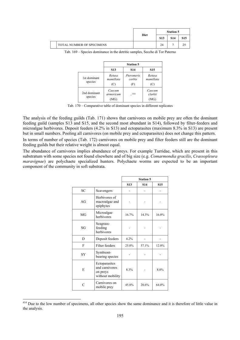
195

Diet

Station 5

S13 S14 S15

TOTAL NUMBER OF SPECIMENS 24 7 25

Tab. 169 – Species dominance in the detritic samples, Secche di Tor Paterno

Station 5 S13 S14 S15

1st dominant species

Retusa mamillata

(C)

Pteromeris corbis

(F)

Retusa mamillata

(C)

2nd dominant species

Caecum armoricum

(MG) - 414

Caecum clarkii (MG)

Tab. 170 – Comparative table of dominant species in different replicates

The analysis of the feeding guilds (Tab. 171) shows that carnivores on mobile prey are often the dominant feeding guild (samples S13 and S15, and the second most abundant in S14), followed by filter-feeders and microalgae herbivores. Deposit feeders (4.2% in S13) and ectoparasites (maximum 8.3% in S13) are present but in small numbers. Pooling all carnivores (on mobile prey and ectoparasites) does not change this pattern. In terms of number of species (Tab. 172) carnivores on mobile prey and filter feeders still are the dominant feeding guilds but their relative weight is almost equal. The abundance of carnivores implies abundance of preys. For example Turridae, which are present in this substratum with some species not found elsewhere and of big size (e.g. Comarmondia gracilis, Crassopleura maravignae) are polychaete specialized hunters. Polychaete worms are expected to be an important component of the community in soft substrata.

Station 5

S13 S14 S15

SC Scavengers - - -

AG Herbivores of macroalgae and epiphytes

- - -

MG Microalgae herbivores 16.7% 14.3% 16.0%

SG Seagrass-feeding herbivores

- - -

D Deposit feeders 4.2% - -

F Filter feeders 25.0% 57.1% 12.0%

SY Symbiont-bearing species - - -

E

Ectoparasites and carnivores on preys without mobility

8.3% - 8.0%

C Carnivores on mobile prey 45.8% 28.6% 64.0%

414 Due to the low number of specimens, all other species show the same dominance and it is therefore of little value in the analysis.

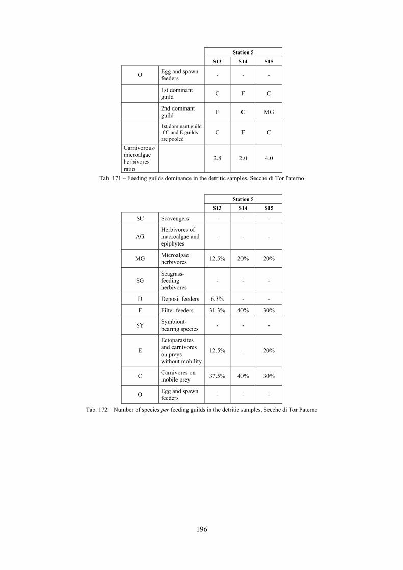
196

Station 5

S13 S14 S15

O Egg and spawn feeders - - -

1st dominant guild C F C

2nd dominant guild F C MG

1st dominant guild if C and E guilds are pooled

C F C

Carnivorous/ microalgae herbivores ratio

2.8 2.0 4.0

Tab. 171 – Feeding guilds dominance in the detritic samples, Secche di Tor Paterno

Station 5

S13 S14 S15

SC Scavengers - - -

AG Herbivores of macroalgae and epiphytes

- - -

MG Microalgae herbivores 12.5% 20% 20%

SG Seagrass-feeding herbivores

- - -

D Deposit feeders 6.3% - -

F Filter feeders 31.3% 40% 30%

SY Symbiont-bearing species - - -

E

Ectoparasites and carnivores on preys without mobility

12.5% - 20%

C Carnivores on mobile prey 37.5% 40% 30%

O Egg and spawn feeders - - -

Tab. 172 – Number of species per feeding guilds in the detritic samples, Secche di Tor Paterno

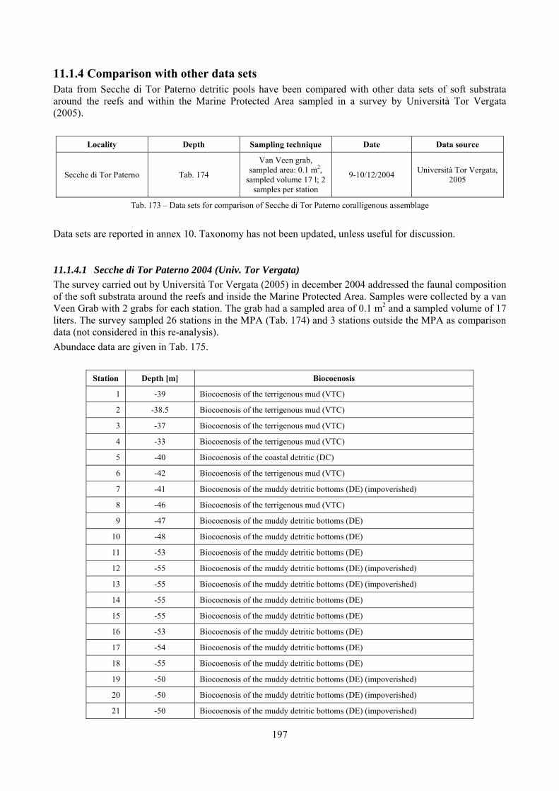
197

11.1.4 Comparison with other data sets Data from Secche di Tor Paterno detritic pools have been compared with other data sets of soft substrata around the reefs and within the Marine Protected Area sampled in a survey by Università Tor Vergata (2005).

Locality Depth Sampling technique Date Data source

Secche di Tor Paterno Tab. 174

Van Veen grab, sampled area: 0.1 m2,

sampled volume 17 l; 2 samples per station

9-10/12/2004 Università Tor Vergata, 2005

Tab. 173 – Data sets for comparison of Secche di Tor Paterno coralligenous assemblage

Data sets are reported in annex 10. Taxonomy has not been updated, unless useful for discussion.

11.1.4.1 Secche di Tor Paterno 2004 (Univ. Tor Vergata) The survey carried out by Università Tor Vergata (2005) in december 2004 addressed the faunal composition of the soft substrata around the reefs and inside the Marine Protected Area. Samples were collected by a van Veen Grab with 2 grabs for each station. The grab had a sampled area of 0.1 m2 and a sampled volume of 17 liters. The survey sampled 26 stations in the MPA (Tab. 174) and 3 stations outside the MPA as comparison data (not considered in this re-analysis). Abundace data are given in Tab. 175.

Station Depth [m] Biocoenosis

1 -39 Biocoenosis of the terrigenous mud (VTC)

2 -38.5 Biocoenosis of the terrigenous mud (VTC)

3 -37 Biocoenosis of the terrigenous mud (VTC)

4 -33 Biocoenosis of the terrigenous mud (VTC)

5 -40 Biocoenosis of the coastal detritic (DC)

6 -42 Biocoenosis of the terrigenous mud (VTC)

7 -41 Biocoenosis of the muddy detritic bottoms (DE) (impoverished)

8 -46 Biocoenosis of the terrigenous mud (VTC)

9 -47 Biocoenosis of the muddy detritic bottoms (DE)

10 -48 Biocoenosis of the muddy detritic bottoms (DE)

11 -53 Biocoenosis of the muddy detritic bottoms (DE)

12 -55 Biocoenosis of the muddy detritic bottoms (DE) (impoverished)

13 -55 Biocoenosis of the muddy detritic bottoms (DE) (impoverished)

14 -55 Biocoenosis of the muddy detritic bottoms (DE)

15 -55 Biocoenosis of the muddy detritic bottoms (DE)

16 -53 Biocoenosis of the muddy detritic bottoms (DE)

17 -54 Biocoenosis of the muddy detritic bottoms (DE)

18 -55 Biocoenosis of the muddy detritic bottoms (DE)

19 -50 Biocoenosis of the muddy detritic bottoms (DE) (impoverished)

20 -50 Biocoenosis of the muddy detritic bottoms (DE) (impoverished)

21 -50 Biocoenosis of the muddy detritic bottoms (DE) (impoverished)

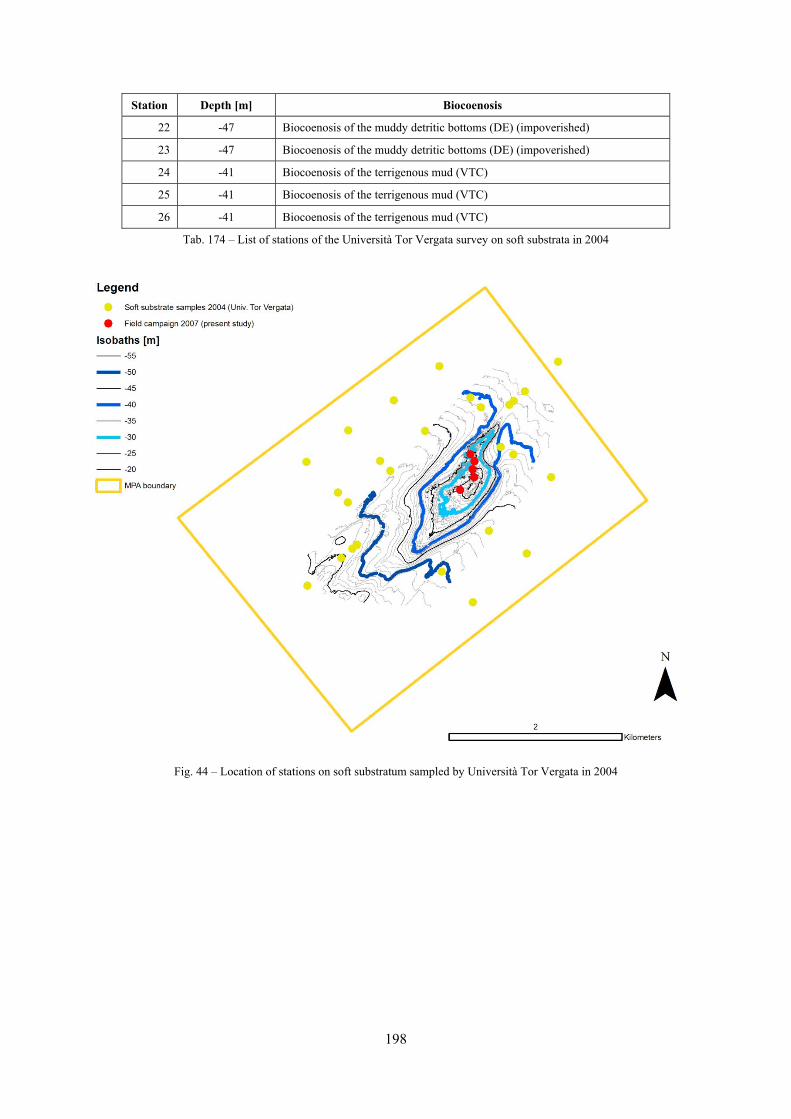
198

Station Depth [m] Biocoenosis

22 -47 Biocoenosis of the muddy detritic bottoms (DE) (impoverished)

23 -47 Biocoenosis of the muddy detritic bottoms (DE) (impoverished)

24 -41 Biocoenosis of the terrigenous mud (VTC)

25 -41 Biocoenosis of the terrigenous mud (VTC)

26 -41 Biocoenosis of the terrigenous mud (VTC)

Tab. 174 – List of stations of the Università Tor Vergata survey on soft substrata in 2004

Fig. 44 – Location of stations on soft substratum sampled by Università Tor Vergata in 2004

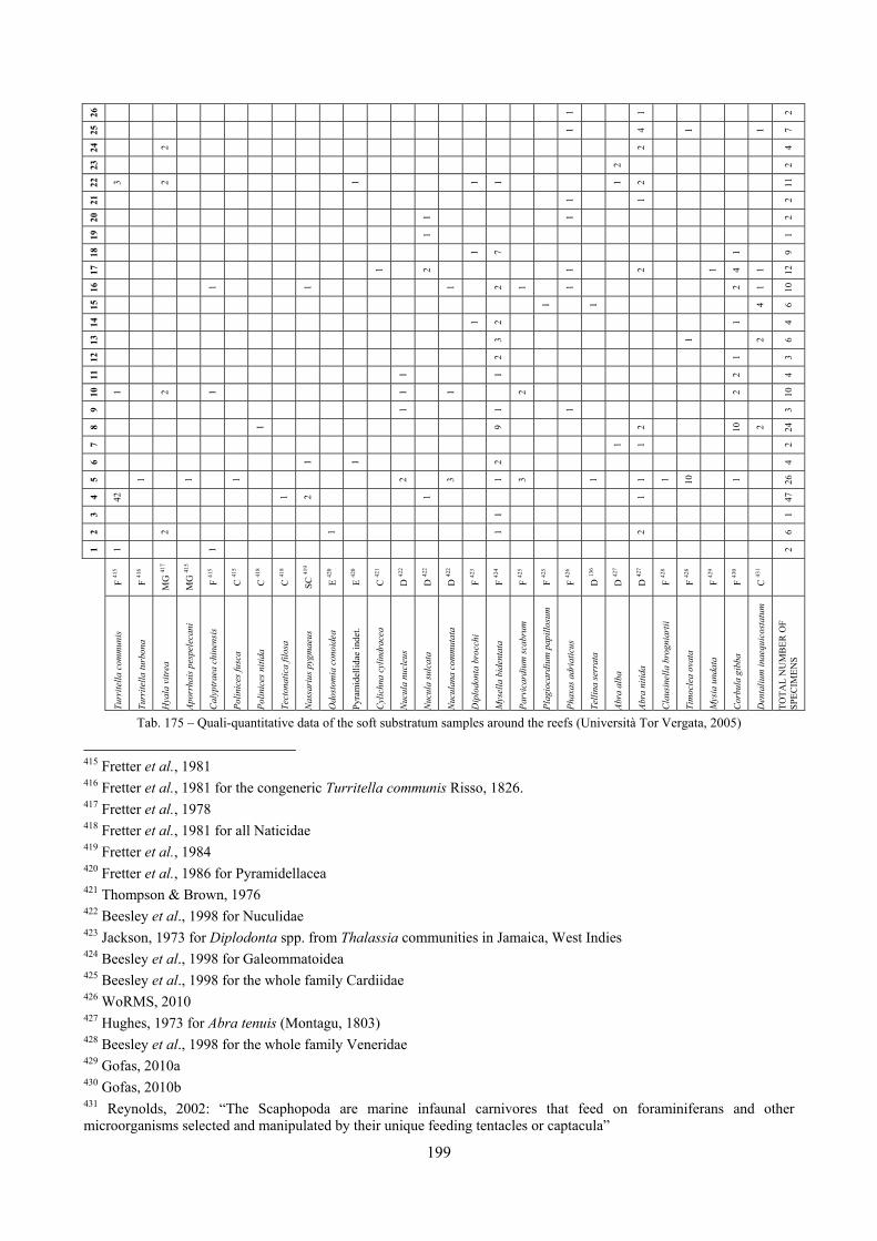
199

26 1 1 2

25 1 4 1 1 7

24 2 2 4

23 2 2

22

3 2 1 1 1 1 2 11

21 1 1 2

20 1 1 2

19 1 1

18 1 7 1 9

17 1 2 1 2 1 4 1 12

16 1 1 1 2 1 1 2 1 10

15 1 1 4 6

14 1 2 1 4

13 3 1 2 6

12 2 1 3

11 1 1 2 4

10

1 2 1 1 1 2 2 10

9 1 1 1 3

8 1 9 2 10

2 24

7 1 1 2

6 1 1 2 4

5 1 1 1 2 3 1 3 1 1 1 10 1 26

4 42 1 2 1 1 47

3 1 1

2 2 1 1 2 6

1 1 1 2

F 41

5

F 41

6

MG

417

MG

415

F 41

5

C 41

5

C 41

8

C 41

8

SC 41

9

E 42

0

E 42

0

C 42

1

D 42

2

D 42

2

D 42

2

F 42

3

F 42

4

F 42

5

F 42

5

F 42

6

D 13

6

D 42

7

D 42

7

F 42

8

F 42

8

F 42

9

F 43

0

C 43

1

Turr

itella

com

mun

is

Turr

itella

turb

ona

Hya

la v

itrea

Apor

rhai

s pes

pele

cani

Cal

yptr

aea

chin

ensi

s

Polin

ices

fusc

a

Polin

ices

niti

da

Tect

onat

ica

filos

a

Nas

sari

us p

ygm

aeus

Odo

stom

ia c

onoi

dea

Pyra

mid

ellid

ae in

det.

Cyl

ichn

a cy

lindr

acea

Nuc

ula

nucl

eus

Nuc

ula

sulc

ata

Nuc

ulan

a co

mm

utat

a

Dip

lodo

nta

broc

chi

Mys

ella

bid

enta

ta

Parv

icar

dium

scab

rum

Plag

ioca

rdiu

m p

apill

osum

Phax

as a

dria

ticus

Telli

na se

rrat

a

Abra

alb

a

Abra

niti

da

Cla

usin

ella

bro

gnia

rtii

Tim

ocle

a ov

ata

Mys

ia u

ndat

a

Cor

bula

gib

ba

Den

taliu

m in

aequ

icos

tatu

m

TOTA

L N

UM

BER

OF

SPEC

IMEN

S

Tab. 175 – Quali-quantitative data of the soft substratum samples around the reefs (Università Tor Vergata, 2005)

415 Fretter et al., 1981 416 Fretter et al., 1981 for the congeneric Turritella communis Risso, 1826. 417 Fretter et al., 1978 418 Fretter et al., 1981 for all Naticidae 419 Fretter et al., 1984 420 Fretter et al., 1986 for Pyramidellacea 421 Thompson & Brown, 1976 422 Beesley et al., 1998 for Nuculidae 423 Jackson, 1973 for Diplodonta spp. from Thalassia communities in Jamaica, West Indies 424 Beesley et al., 1998 for Galeommatoidea 425 Beesley et al., 1998 for the whole family Cardiidae 426 WoRMS, 2010 427 Hughes, 1973 for Abra tenuis (Montagu, 1803) 428 Beesley et al., 1998 for the whole family Veneridae 429 Gofas, 2010a 430 Gofas, 2010b 431 Reynolds, 2002: “The Scaphopoda are marine infaunal carnivores that feed on foraminiferans and other microorganisms selected and manipulated by their unique feeding tentacles or captacula”

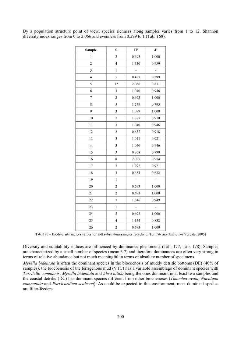
200

By a population structure point of view, species richness along samples varies from 1 to 12. Shannon diversity index ranges from 0 to 2.066 and evenness from 0.299 to 1 (Tab. 168).

Sample S H' J'

1 2 0.693 1.000

2 4 1.330 0.959

3 1 - -

4 5 0.481 0.299

5 12 2.066 0.831

6 3 1.040 0.946

7 2 0.693 1.000

8 5 1.279 0.795

9 3 1.099 1.000

10 7 1.887 0.970

11 3 1.040 0.946

12 2 0.637 0.918

13 3 1.011 0.921

14 3 1.040 0.946

15 3 0.868 0.790

16 8 2.025 0.974

17 7 1.792 0.921

18 3 0.684 0.622

19 1 - -

20 2 0.693 1.000

21 2 0.693 1.000

22 7 1.846 0.949

23 1 - -

24 2 0.693 1.000

25 4 1.154 0.832

26 2 0.693 1.000

Tab. 176 – Biodiversity indices values for soft substratum samples, Secche di Tor Paterno (Univ. Tor Vergata, 2005)

Diversity and equitability indices are influenced by dominance phenomena (Tab. 177, Tab. 178). Samples are characterized by a small number of species (mean 3.7) and therefore dominances are often very strong in terms of relative abundance but not much meaningful in terms of absolute number of specimens. Mysella bidentata is often the dominant species in the biocoenosis of muddy detritic bottoms (DE) (40% of samples), the biocoenosis of the terrigenous mud (VTC) has a variable assemblage of dominant species with Turritella communis, Mysella bidentata and Abra nitida being the ones dominant in at least two samples and the coastal detritic (DC) has dominant species different from other biocoenoses (Timoclea ovata, Nuculana commutata and Parvicardium scabrum). As could be expected in this environment, most dominant species are filter-feeders.

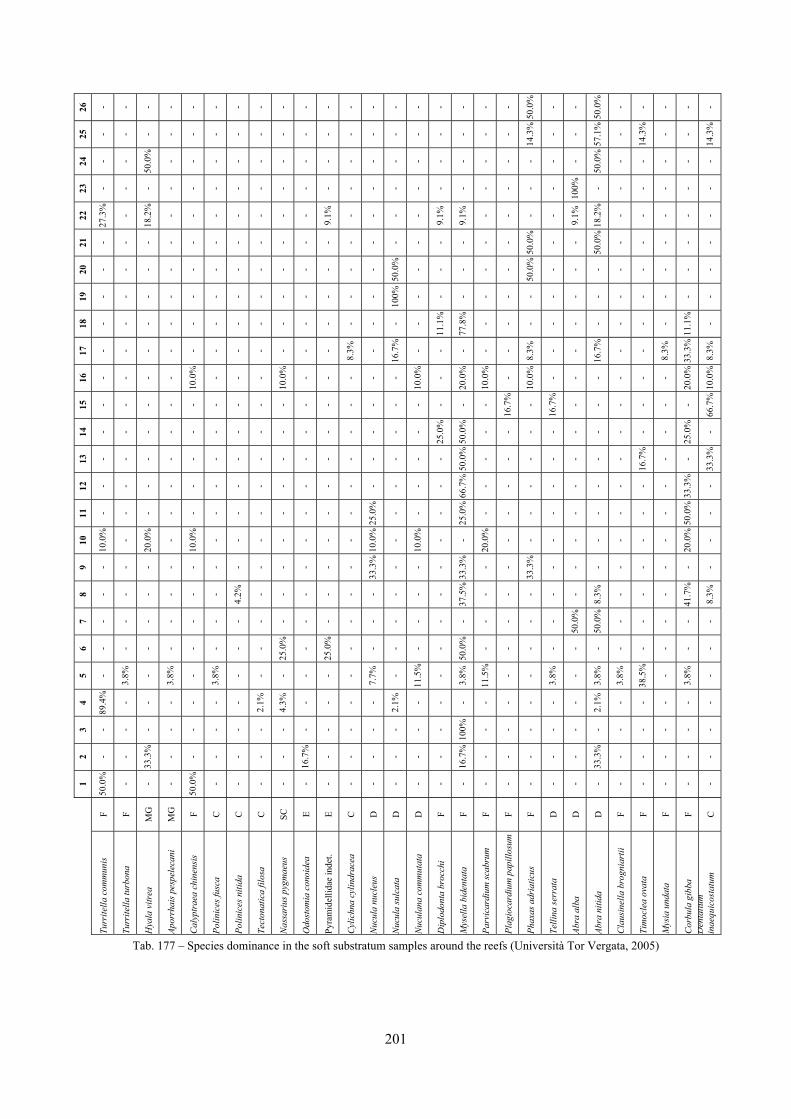
201

26

- - - - - - - - - - - - - - - - - - -

50.0

%

- -

50.0

%

- - - - -

25

- - - - - - - - - - - - - - - - - - -

14.3

%

- -

57.1

%

-

14.3

%

- -

14.3

%

24

- -

50.0

%

- - - - - - - - - - - - - - - - - - -

50.0

%

- - - - -

23

- - - - - - - - - - - - - - - - - - - - -

100%

- - - - - -

22

27.3

%

-

18.2

%

- - - - - - -

9.1%

- - - -

9.1%

9.1%

- - - -

9.1%

18.2

%

- - - - -

21

- - - - - - - - - - - - - - - - - - -

50.0

%

- -

50.0

%

- - - - -

20

- - - - - - - - - - - - -

50.0

%

- - - - -

50.0

%

- - - - - - - -

19

- - - - - - - - - - - - -

100%

- - - - - - - - - - - - - -

18

- - - - - - - - - - - - - - -

11.1

%

77.8

%

- - - - - - - - -

11.1

%

-

17

- - - - - - - - - - -

8.3%

-

16.7

%

- - - - -

8.3%

- -

16.7

%

- -

8.3%

33.3

%

8.3%

16

- - - -

10.0

%

- - -

10.0

%

- - - - -

10.0

%

-

20.0

%

10.0

%

-

10.0

%

- - - - - -

20.0

%

10.0

%

15

- - - - - - - - - - - - - - - - - -

16.7

%

-

16.7

%

- - - - - -

66.7

%

14

- - - - - - - - - - - - - - -

25.0

%

50.0

%

- - - - - - - - -

25.0

%

-

13

- - - - - - - - - - - - - - - -

50.0

%

- - - - - - -

16.7

%

- -

33.3

%

12

- - - - - - - - - - - - - - - -

66.7

%

- - - - - - - - -

33.3

%

-

11

- - - - - - - - - - - -

25.0

%

- - -

25.0

%

- - - - - - - - -

50.0

%

-

10

10.0

%

-

20.0

%

-

10.0

%

- - - - - - -

10.0

%

-

10.0

%

- -

20.0

%

- - - - - - - -

20.0

%

-

9 - - - - - - - - - - - -

33.3

%

- - -

33.3

%

- -

33.3

%

- - - - - - - -

8 - - - - - -

4.2%

- - - - - - - - -

37.5

%

- - - - -

8.3%

- - -

41.7

%

8.3%

7 - - - - - - - - - - - - - - - - - - - - -

50.0

%

50.0

%

- - - - -

6 - - - - - - - -

25.0

%

-

25.0

%

- - - - -

50.0

%

- - - - - - - - - - -

5 -

3.8%

-

3.8%

-

3.8%

- - - - - -

7.7%

-

11.5

%

-

3.8%

11.5

%

- -

3.8%

-

3.8%

3.8%

38.5

%

-

3.8%

-

4

89.4

%

- - - - - -

2.1%

4.3%

- - - -

2.1%

- - - - - - - -

2.1%

- - - - -

3 - - - - - - - - - - - - - - - -

100%

- - - - - - - - - - -

2 - -

33.3

%

- - - - - -

16.7

%

- - - - - -

16.7

%

- - - - -

33.3

%

- - - - -

1

50.0

%

- - -

50.0

%

- - - - - - - - - - - - - - - - - - - - - - -

F

F

MG

MG

F C

C

C

SC

E

E

C

D

D

D F

F

F

F F

D

D

D F

F

F

F

C

Turr

itella

com

mun

is

Turr

itella

turb

ona

Hya

la v

itrea

Apor

rhai

s pes

pele

cani

Cal

yptr

aea

chin

ensi

s

Polin

ices

fusc

a

Polin

ices

niti

da

Tect

onat

ica

filos

a

Nas

sari

us p

ygm

aeus

Odo

stom

ia c

onoi

dea

Pyra

mid

ellid

ae in

det.

Cyl

ichn

a cy

lindr

acea

Nuc

ula

nucl

eus

Nuc

ula

sulc

ata

Nuc

ulan

a co

mm

utat

a

Dip

lodo

nta

broc

chi

Mys

ella

bid

enta

ta

Parv

icar

dium

scab

rum

Plag

ioca

rdiu

m p

apill

osum

Phax

as a

dria

ticus

Telli

na se

rrat

a

Abra

alb

a

Abra

niti

da

Cla

usin

ella

bro

gnia

rtii

Tim

ocle

a ov

ata

Mys

ia u

ndat

a

Cor

bula

gib

ba

Den

taliu

m

inae

quic

osta

tum

Tab. 177 – Species dominance in the soft substratum samples around the reefs (Università Tor Vergata, 2005)

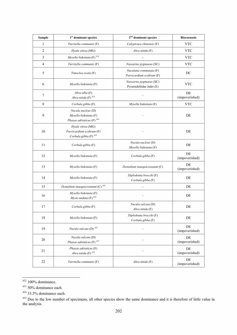
202

Sample 1st dominant species 2nd dominant species Biocoenosis

1 Turritella communis (F) Calyptraea chinensis (F) VTC

2 Hyala vitrea (MG) Abra nitida (F) VTC

3 Mysella bidentata (F) 432 - VTC

4 Turritella communis (F) Nassarius pygmaeus (SC) VTC

5 Timoclea ovata (F) Nuculana commutata (F)

Parvicardium scabrum (F) DC

6 Mysella bidentata (F) Nassarius pygmaeus (SC) Pyramidellidae indet (E)

VTC

7 Abra alba (F)

Abra nitida (F) 433 - DE

(impoverished)

8 Corbula gibba (F) Mysella bidentata (F) VTC

9 Nucula nucleus (D)

Mysella bidentata (F) Phaxas adriaticus (F) 434

- DE

10 Hyala vitrea (MG)

Parvicardium scabrum (F) Corbula gibba (F) 435

- DE

11 Corbula gibba (F) Nucula nucleus (D)

Mysella bidentata (F) DE

12 Mysella bidentata (F) Corbula gibba (F) DE (impoverished)

13 Mysella bidentata (F) Dentalium inaequicostatum (C) DE (impoverished)

14 Mysella bidentata (F) Diplodonta brocchi (F)

Corbula gibba (F) DE

15 Dentalium inaequicostatum (C) 435 - DE

16 Mysella bidentata (F) Mysia undata (F) 435

- DE

17 Corbula gibba (F) Nucula sulcata (D)

Abra nitida (F) DE

18 Mysella bidentata (F) Diplodonta brocchi (F)

Corbula gibba (F) DE

19 Nucula sulcata (D) 432 - DE (impoverished)

20 Nucula sulcata (D)

Phaxas adriaticus (F) 433 - DE

(impoverished)

21 Phaxas adriaticus (F)

Abra nitida (F) 433 - DE

(impoverished)

22 Turritella communis (F) Abra nitida (F) DE (impoverished)

432 100% dominance. 433 50% dominance each. 434 33.3% dominance each. 435 Due to the low number of specimens, all other species show the same dominance and it is therefore of little value in the analysis.

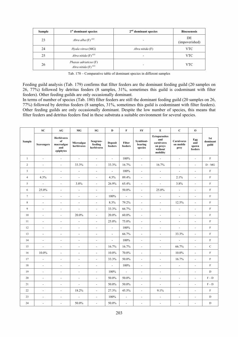
203

Sample 1st dominant species 2nd dominant species Biocoenosis

23 Abra alba (F) 432 - DE (impoverished)

24 Hyala vitrea (MG) Abra nitida (F) VTC

25 Abra nitida (F) 435 - VTC

26 Phaxas adriaticus (F)

Abra nitida (F) 433 - VTC

Tab. 178 – Comparative table of dominant species in different samples

Feeding guild analysis (Tab. 179) confirms that filter feeders are the dominant feeding guild (20 samples on 26, 77%) followed by detritus feeders (8 samples, 31%, sometimes this guild is codominant with filter feeders). Other feeding guilds are only occasionally dominant. In terms of number of species (Tab. 180) filter feeders are still the dominant feeding guild (20 samples on 26, 77%) followed by detritus feeders (8 samples, 31%, sometimes this guild is codominant with filter feeders). Other feeding guilds are only occasionally dominant. Despite the low number of species, this means that filter feeders and detritus feeders find in these substrata a suitable environment for several species.

Sample

SC AG MG SG D F SY E C O

1st dominant

guild Scavengers

Herbivores of

macroalgae and

epiphytes

Microalgae herbivores

Seagrass-feeding

herbivores

Deposit feeders

Filter feeders

Symbiont-bearing species

Ectoparasites and

carnivores on preys without mobility

Carnivores on mobile

prey

Egg and

spawn feeders

1 - - - - - 100% - - - - F

2 - - 33.3% - 33.3% 16.7% - 16.7% - - D – MG

3 - - - - - 100% - - - - F

4 4.3% - - - 4.3% 89.4% - - 2.1% - F

5 - - 3.8% - 26.9% 65.4% - - 3.8% - F

6 25.0% - - - - 50.0% - 25.0% - - F

7 - - - - 100% - - - - - F

8 - - - - 8.3% 79.2% - - 12.5% - F

9 - - - - 33.3% 66.7% - - - - F

10 - - 20.0% - 20.0% 60.0% - - - - F

11 - - - - 25.0% 75.0% - - - - F

12 - - - - - 100% - - - - F

13 - - - - - 66.7% - - 33.3% - F

14 - - - - - 100% - - - - F

15 - - - - 16.7% 16.7% - - 66.7% - C

16 10.0% - - - 10.0% 70.0% - - 10.0% - F

17 - - - - 33.3% 50.0% - - 16.7% - F

18 - - - - - 100% - - - - F

19 - - - - 100% - - - - - D

20 - - - - 50.0% 50.0% - - - - F – D

21 - - - - 50.0% 50.0% - - - - F – D

22 - - 18.2% - 27.3% 45.5% - 9.1% - - F

23 - - - - 100% - - - - - D

24 - - 50.0% - 50.0% - - - - - D

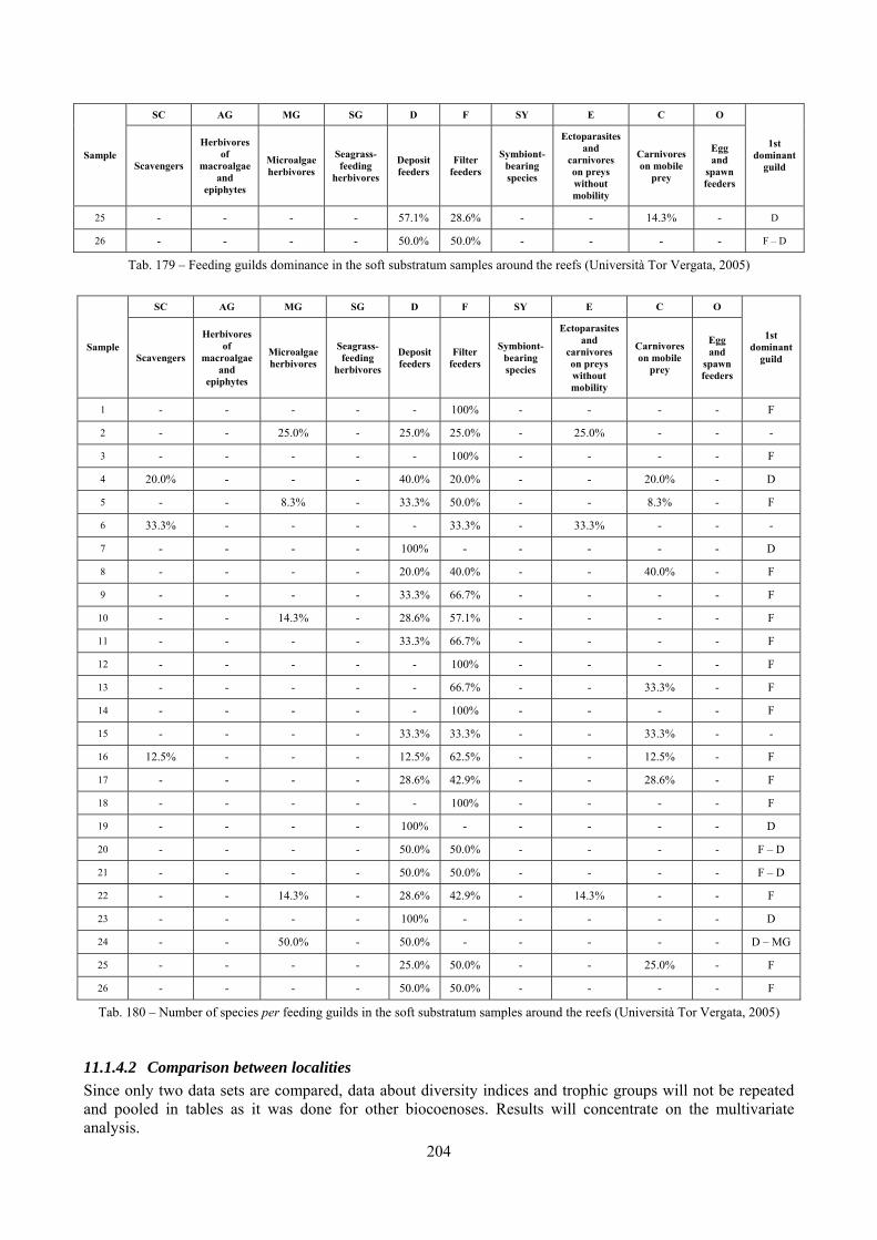
204

Sample

SC AG MG SG D F SY E C O

1st dominant

guild Scavengers

Herbivores of

macroalgae and

epiphytes

Microalgae herbivores

Seagrass-feeding

herbivores

Deposit feeders

Filter feeders

Symbiont-bearing species

Ectoparasites and

carnivores on preys without mobility

Carnivores on mobile

prey

Egg and

spawn feeders

25 - - - - 57.1% 28.6% - - 14.3% - D

26 - - - - 50.0% 50.0% - - - - F – D

Tab. 179 – Feeding guilds dominance in the soft substratum samples around the reefs (Università Tor Vergata, 2005)

Sample

SC AG MG SG D F SY E C O

1st dominant

guild Scavengers

Herbivores of

macroalgae and

epiphytes

Microalgae herbivores

Seagrass-feeding

herbivores

Deposit feeders

Filter feeders

Symbiont-bearing species

Ectoparasites and

carnivores on preys without mobility

Carnivores on mobile

prey

Egg and

spawn feeders

1 - - - - - 100% - - - - F

2 - - 25.0% - 25.0% 25.0% - 25.0% - - -

3 - - - - - 100% - - - - F

4 20.0% - - - 40.0% 20.0% - - 20.0% - D

5 - - 8.3% - 33.3% 50.0% - - 8.3% - F

6 33.3% - - - - 33.3% - 33.3% - - -

7 - - - - 100% - - - - - D

8 - - - - 20.0% 40.0% - - 40.0% - F

9 - - - - 33.3% 66.7% - - - - F

10 - - 14.3% - 28.6% 57.1% - - - - F

11 - - - - 33.3% 66.7% - - - - F

12 - - - - - 100% - - - - F

13 - - - - - 66.7% - - 33.3% - F

14 - - - - - 100% - - - - F

15 - - - - 33.3% 33.3% - - 33.3% - -

16 12.5% - - - 12.5% 62.5% - - 12.5% - F

17 - - - - 28.6% 42.9% - - 28.6% - F

18 - - - - - 100% - - - - F

19 - - - - 100% - - - - - D

20 - - - - 50.0% 50.0% - - - - F – D

21 - - - - 50.0% 50.0% - - - - F – D

22 - - 14.3% - 28.6% 42.9% - 14.3% - - F

23 - - - - 100% - - - - - D

24 - - 50.0% - 50.0% - - - - - D – MG

25 - - - - 25.0% 50.0% - - 25.0% - F

26 - - - - 50.0% 50.0% - - - - F

Tab. 180 – Number of species per feeding guilds in the soft substratum samples around the reefs (Università Tor Vergata, 2005)

11.1.4.2 Comparison between localities Since only two data sets are compared, data about diversity indices and trophic groups will not be repeated and pooled in tables as it was done for other biocoenoses. Results will concentrate on the multivariate analysis.

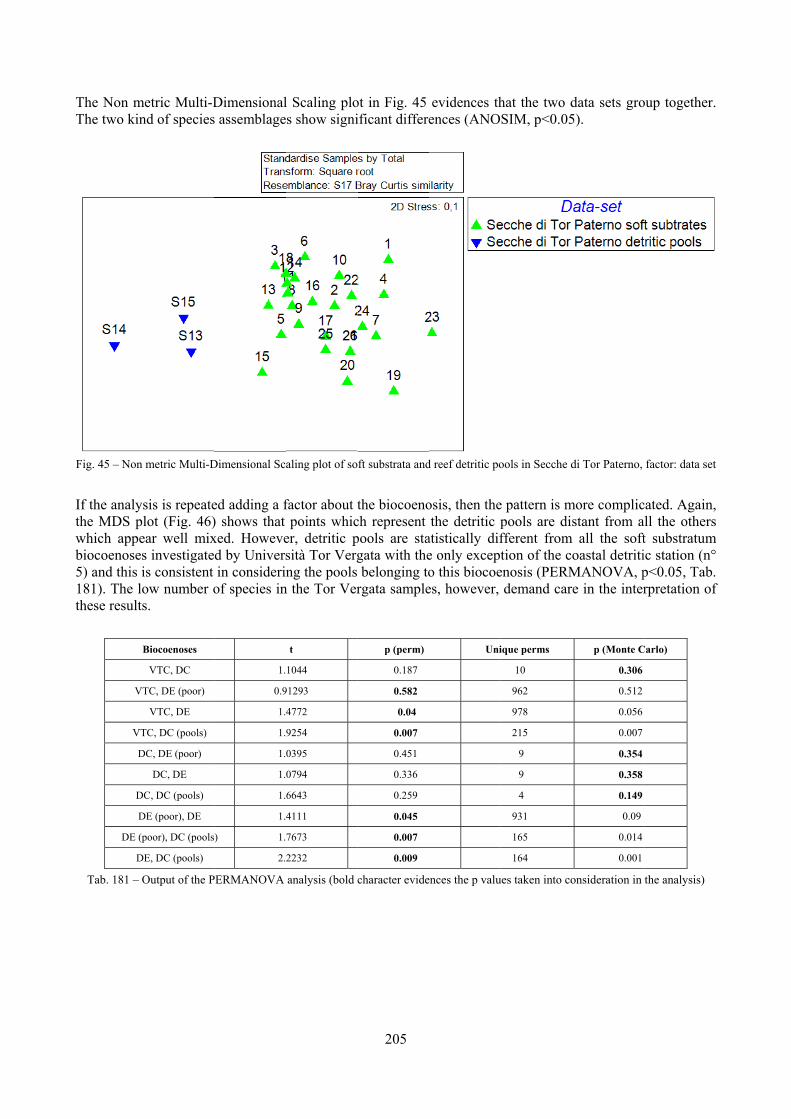
The Non mThe two kin

Fig. 45 – Non

If the analythe MDS pwhich appebiocoenoses5) and this i181). The lothese results

B

VT

VT

D

D

D

DE (p

D

Tab. 181 – O

metric Multi-Dnd of species

metric Multi-D

sis is repeatelot (Fig. 46)

ear well mixs investigateis consistent ow number os.

Biocoenoses

VTC, DC

TC, DE (poor)

VTC, DE

TC, DC (pools)

DC, DE (poor)

DC, DE

DC, DC (pools)

DE (poor), DE

poor), DC (pools

DE, DC (pools)

Output of the P

Dimensionals assemblage

Dimensional Sc

ed adding a f) shows that xed. Howeved by Universin considerin

of species in

1.

0.9

1.

1.

1.

1.

1.

1.

) 1.

2.

PERMANOVA

l Scaling plos show signi

aling plot of so

factor about tpoints whic

er, detritic psità Tor Vergng the pools

n the Tor Ver

t

1044

91293

4772

9254

0395

0794

6643

4111

7673

2232

analysis (bold

205

ot in Fig. 45ificant differe

ft substrata and

the biocoenoch represent pools are stagata with thebelonging to

rgata sample

p (perm)

0.187

0.582

0.04

0.007

0.451

0.336

0.259

0.045

0.007

0.009

character evide

evidences thences (ANO

d reef detritic po

osis, then thethe detritic p

atistically dife only excepo this biocoees, however,

Uni

ences the p valu

hat the two dSIM, p<0.05

ools in Secche d

e pattern is mpools are different fromtion of the c

enosis (PERMdemand car

ique perms

10

962

978

215

9

9

4

931

165

164

ues taken into co

data sets gro5).

di Tor Paterno,

more complicstant from a

m all the softoastal detriti

MANOVA, pre in the inter

p (Monte C

0.306

0.512

0.056

0.007

0.354

0.358

0.149

0.09

0.014

0.001

onsideration in

oup together.

factor: data set

cated. Again,all the otherst substratumic station (n°p<0.05, Tab.rpretation of

Carlo)

the analysis)

.

t

, s

m ° . f

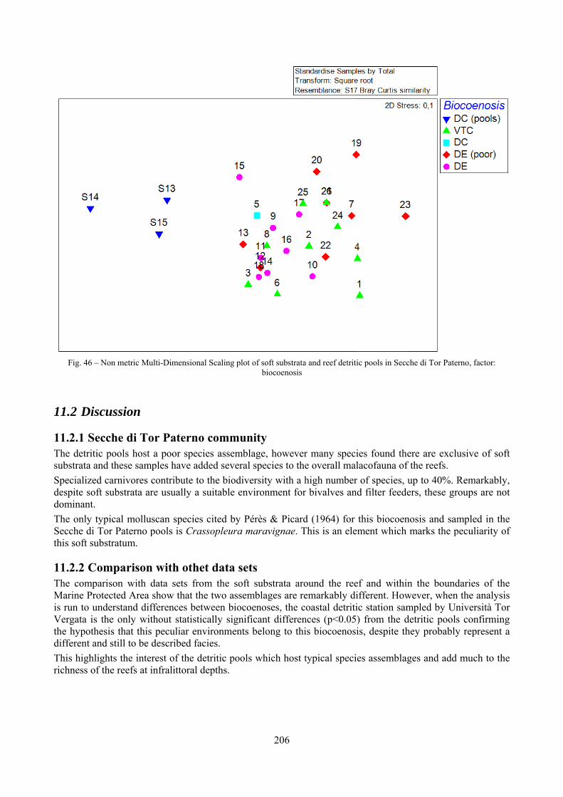
Fig. 46 – N

11.2 Disc

11.2.1 SecThe detriticsubstrata anSpecialized despite softdominant. The only tySecche di Tthis soft sub

11.2.2 CoThe compaMarine Protis run to unVergata is tthe hypothedifferent anThis highligrichness of

Non metric Mu

cussion

cche di Toc pools host nd these samp

carnivores ct substrata ar

ypical mollusTor Paterno pbstratum.

omparisonarison with dtected Area s

nderstand difthe only witesis that this nd still to be dghts the interthe reefs at i

ulti-Dimensiona

or Paternoa poor speciples have adcontribute tore usually a s

scan species pools is Cras

with othedata sets froshow that th

fferences betwthout statistic

peculiar envdescribed facrest of the denfralittoral d

al Scaling plot o

o communiies assembladed several s

o the biodiversuitable envi

cited by Péssopleura ma

et data setsom the soft se two assemween biocoecally significvironments bcies. etritic pools depths.

206

of soft substratabiocoenosis

ity age, howeverspecies to thersity with a hironment for

rès & Picardaravignae. T

s substrata aro

mblages are reenoses, the ccant differenbelong to thi

which host t

a and reef detrit

r many specie overall malhigh numberr bivalves an

d (1964) for This is an ele

ound the reeemarkably dioastal detriti

nces (p<0.05is biocoenos

typical speci

ic pools in Secc

ies found thlacofauna ofr of species, nd filter feede

this biocoenement which

ef and withiifferent. Howic station sam) from the dis, despite th

ies assemblag

che di Tor Pater

ere are excluf the reefs. up to 40%. Rers, these gr

nosis and sammarks the p

n the boundwever, when mpled by Undetritic poolshey probably

ges and add

rno, factor:

usive of soft

Remarkably,oups are not

mpled in thepeculiarity of

daries of thethe analysis

niversità Tors confirmingy represent a

much to the

t

, t

e f

e s r g a

e

207

12 Agreement between death and living molluscs assemblages The study of the agreement between death and life assemblages has two main fields of interest. First, palaeoecological reconstruction of benthic communities is based on the ability to evaluate how accurately death assemblages preserve the composition and structure of the original community. Second, the evaluation of biodiversity of an area is a basic requirement for any conservation activity. Biodiversity surveys require time in order to sample enough all the biocoenoses and would require multiple surveys in different seasons and years to fully intercept all the organisms living in the area which is generally not done due to financial and operational constraints. Since death assemblages accumulate and preserve specimens of several seasons and years due to the phenomenon of “time-averaging”, they may describe the biodiversity of an area in a more complete way and with a reduced effort. Moreover, this would be a virtually totally non-destructive monitoring of the communities since the living specimens in small volumes of sediment are very few. Therefore, it is interesting to evaluate to which extent death assemblages give us information about these issues and with which bias and limitations. Of course, taxa which allow a thorough dead-live comparison are those which produce hard skeletal parts which accumulate after the death of the animal and therefore molluscs perform excellently since most species have a calcareous shell and it is the most diverse animal benthic phylum (in the Mediterranean Sea almost 2,000 species are listed at present; 53,000 have been described worldwide with a yearly increment of 350 species (Bouchet, 2006)). Other groups have calcareous skeletons, but their low diversity in present day communities (e.g. Brachiopoda) or their limited geographic distribution (e.g. corals) render their use on a wide scale of lower interest or limited to specific geographic areas. Study of the dead-live agreement for palaeoecological purposes has been mainly carried out on soft substrata. Cadée (1968) compared molluscan biocoenoses and thanatocoenoses in the Ria de Arosa (Galicia, NW Spain); there species found in the biocoenoses were always found in the thanatocoenosis but there was little quantitative correlation between the two. Kidwell (2001) re-analyses 17 molluscan data sets with several conclusions of general interest:

‐ Species that are not present in the death assemblages are virtually all numerically rare and small and/or fragile;

‐ Death assemblages are preferentially composed of species that are known to live locally, those which do not may be exotics or relicts; however, in case of discordances the main reason may be undersampling of the living community;

‐ The rank order of dominance is generally well preserved in death and life assemblages; ‐ The species richness of a death assemblage is generally 2 or 3 times that of the living fauna.

Very few studies have been carried out on molluscs assemblages on hard substrata. Zuschin et al. (2000) studied the issue on coral reef associated hard substrata in the northern Red Sea. Between their main conclusions the good agreement in the taxonomic composition of the death and living assemblages, the observation of strong differences regarding dominating taxa, due to being rapidly over-grown by corals and coralline algae and due to post-mortem transport. Zuschin & Oliver (2003) analyzed this issue on sublittoral hard substrata around granitic islands of the Seychelles. Among their main conclusions there are they support the use of a reduced data set without the quantitatively unimportant species (taxa which contribute less than 1% to either the live or dead mollusc content of all samples); they observe strong differences in the abundance of co-occurring living and dead molluscs mainly due to the phenomenon of post-mortem out-of-habitat transport, which reduces the in-situ abundances, and pagurization, which increases abundances. Among its limitations, the low number of considered taxa, 49 in the full data set, due to sampling strategy which considered only species above 1 cm in size, and the low taxonomic resolution since some groups were identified at the supra-specific level only due to lack of adequate taxonomic knowledge on tropical molluscs (e.g. some bivalves like Chamoidea, Spondylidae, Ostreoidea) and for the difficulties of identify them in the field (e.g. Conus). A single paper was found dealing specifically with the comparison of a quaternary molluscs (gastropods) assemblage from a Posidonia oceanica meadow with a recent living community in the same locality (Russo et al., 1989). Operating with multivariate analysis, they observed time-related differences in the population

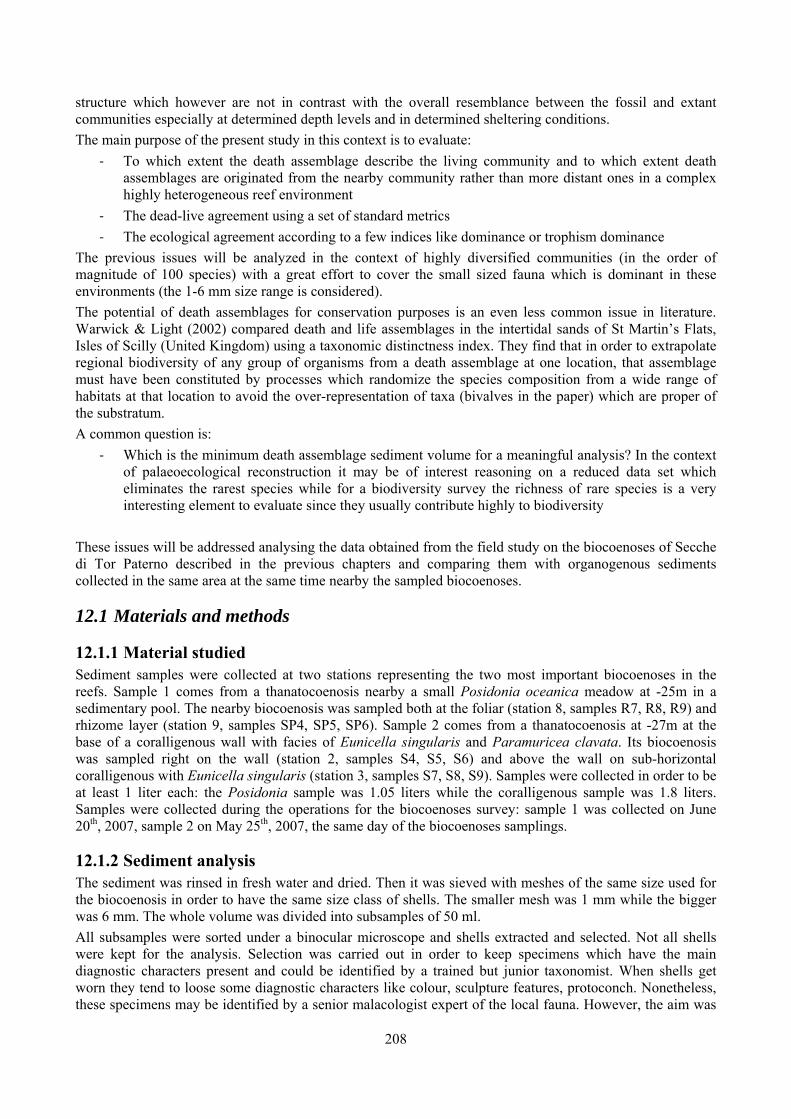
208

structure which however are not in contrast with the overall resemblance between the fossil and extant communities especially at determined depth levels and in determined sheltering conditions. The main purpose of the present study in this context is to evaluate:

‐ To which extent the death assemblage describe the living community and to which extent death assemblages are originated from the nearby community rather than more distant ones in a complex highly heterogeneous reef environment

‐ The dead-live agreement using a set of standard metrics ‐ The ecological agreement according to a few indices like dominance or trophism dominance

The previous issues will be analyzed in the context of highly diversified communities (in the order of magnitude of 100 species) with a great effort to cover the small sized fauna which is dominant in these environments (the 1-6 mm size range is considered). The potential of death assemblages for conservation purposes is an even less common issue in literature. Warwick & Light (2002) compared death and life assemblages in the intertidal sands of St Martin’s Flats, Isles of Scilly (United Kingdom) using a taxonomic distinctness index. They find that in order to extrapolate regional biodiversity of any group of organisms from a death assemblage at one location, that assemblage must have been constituted by processes which randomize the species composition from a wide range of habitats at that location to avoid the over-representation of taxa (bivalves in the paper) which are proper of the substratum. A common question is:

‐ Which is the minimum death assemblage sediment volume for a meaningful analysis? In the context of palaeoecological reconstruction it may be of interest reasoning on a reduced data set which eliminates the rarest species while for a biodiversity survey the richness of rare species is a very interesting element to evaluate since they usually contribute highly to biodiversity

These issues will be addressed analysing the data obtained from the field study on the biocoenoses of Secche di Tor Paterno described in the previous chapters and comparing them with organogenous sediments collected in the same area at the same time nearby the sampled biocoenoses.

12.1 Materials and methods

12.1.1 Material studied Sediment samples were collected at two stations representing the two most important biocoenoses in the reefs. Sample 1 comes from a thanatocoenosis nearby a small Posidonia oceanica meadow at -25m in a sedimentary pool. The nearby biocoenosis was sampled both at the foliar (station 8, samples R7, R8, R9) and rhizome layer (station 9, samples SP4, SP5, SP6). Sample 2 comes from a thanatocoenosis at -27m at the base of a coralligenous wall with facies of Eunicella singularis and Paramuricea clavata. Its biocoenosis was sampled right on the wall (station 2, samples S4, S5, S6) and above the wall on sub-horizontal coralligenous with Eunicella singularis (station 3, samples S7, S8, S9). Samples were collected in order to be at least 1 liter each: the Posidonia sample was 1.05 liters while the coralligenous sample was 1.8 liters. Samples were collected during the operations for the biocoenoses survey: sample 1 was collected on June 20th, 2007, sample 2 on May 25th, 2007, the same day of the biocoenoses samplings.

12.1.2 Sediment analysis The sediment was rinsed in fresh water and dried. Then it was sieved with meshes of the same size used for the biocoenosis in order to have the same size class of shells. The smaller mesh was 1 mm while the bigger was 6 mm. The whole volume was divided into subsamples of 50 ml. All subsamples were sorted under a binocular microscope and shells extracted and selected. Not all shells were kept for the analysis. Selection was carried out in order to keep specimens which have the main diagnostic characters present and could be identified by a trained but junior taxonomist. When shells get worn they tend to loose some diagnostic characters like colour, sculpture features, protoconch. Nonetheless, these specimens may be identified by a senior malacologist expert of the local fauna. However, the aim was

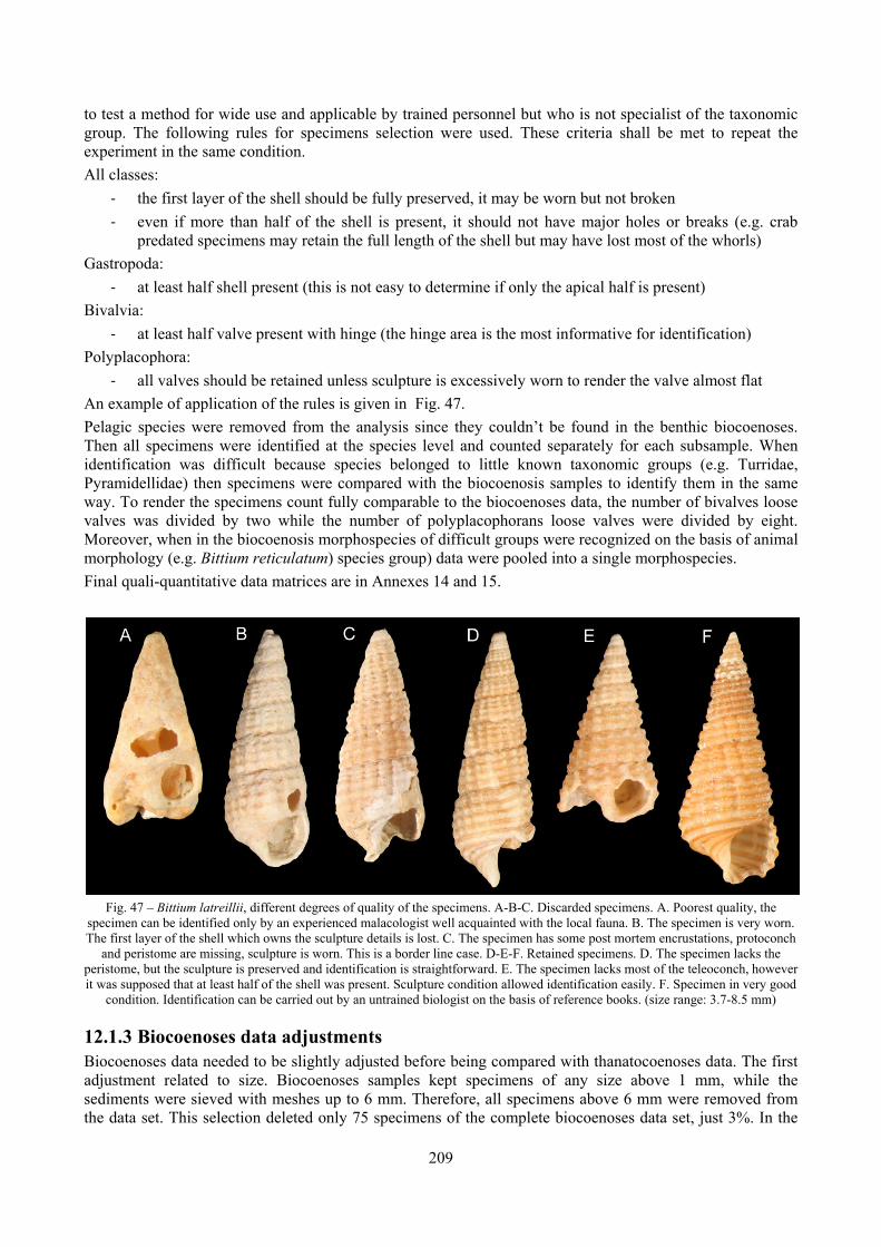
209

to test a method for wide use and applicable by trained personnel but who is not specialist of the taxonomic group. The following rules for specimens selection were used. These criteria shall be met to repeat the experiment in the same condition. All classes:

‐ the first layer of the shell should be fully preserved, it may be worn but not broken ‐ even if more than half of the shell is present, it should not have major holes or breaks (e.g. crab

predated specimens may retain the full length of the shell but may have lost most of the whorls) Gastropoda:

‐ at least half shell present (this is not easy to determine if only the apical half is present) Bivalvia:

‐ at least half valve present with hinge (the hinge area is the most informative for identification) Polyplacophora:

‐ all valves should be retained unless sculpture is excessively worn to render the valve almost flat An example of application of the rules is given in Fig. 47. Pelagic species were removed from the analysis since they couldn’t be found in the benthic biocoenoses. Then all specimens were identified at the species level and counted separately for each subsample. When identification was difficult because species belonged to little known taxonomic groups (e.g. Turridae, Pyramidellidae) then specimens were compared with the biocoenosis samples to identify them in the same way. To render the specimens count fully comparable to the biocoenoses data, the number of bivalves loose valves was divided by two while the number of polyplacophorans loose valves were divided by eight. Moreover, when in the biocoenosis morphospecies of difficult groups were recognized on the basis of animal morphology (e.g. Bittium reticulatum) species group) data were pooled into a single morphospecies. Final quali-quantitative data matrices are in Annexes 14 and 15.

Fig. 47 – Bittium latreillii, different degrees of quality of the specimens. A-B-C. Discarded specimens. A. Poorest quality, the

specimen can be identified only by an experienced malacologist well acquainted with the local fauna. B. The specimen is very worn. The first layer of the shell which owns the sculpture details is lost. C. The specimen has some post mortem encrustations, protoconch

and peristome are missing, sculpture is worn. This is a border line case. D-E-F. Retained specimens. D. The specimen lacks the peristome, but the sculpture is preserved and identification is straightforward. E. The specimen lacks most of the teleoconch, however it was supposed that at least half of the shell was present. Sculpture condition allowed identification easily. F. Specimen in very good

condition. Identification can be carried out by an untrained biologist on the basis of reference books. (size range: 3.7-8.5 mm)

12.1.3 Biocoenoses data adjustments Biocoenoses data needed to be slightly adjusted before being compared with thanatocoenoses data. The first adjustment related to size. Biocoenoses samples kept specimens of any size above 1 mm, while the sediments were sieved with meshes up to 6 mm. Therefore, all specimens above 6 mm were removed from the data set. This selection deleted only 75 specimens of the complete biocoenoses data set, just 3%. In the

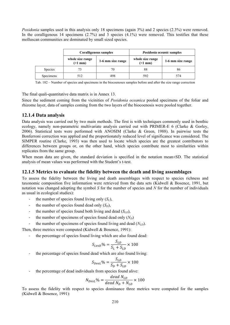
210

Posidonia samples used in this analysis only 18 specimens (again 3%) and 2 species (2.3%) were removed. In the coralligenous 14 specimens (2.7%) and 3 species (4.1%) were removed. This testifies that these molluscan communities are dominated by small sized species.

Coralligenous samples Posidonia oceanic samples

whole size range (>1 mm) 1-6 mm size range whole size range

(>1 mm) 1-6 mm size range

Species 73 70 88 86

Specimens 512 498 592 574

Tab. 182 – Number of species and specimens in the biocoenoses samples before and after the size range correction

The final quali-quantitative data matrix is in Annex 13. Since the sediment coming from the vicinities of Posidonia oceanica pooled specimens of the foliar and rhizome layer, data of samples coming from the two layers of the biocoenosis were pooled together.

12.1.4 Data analysis Data analysis was carried out by two main methods. The first is with techniques commonly used in benthic ecology, namely non-parametric multivariate analysis carried out with PRIMER-E 6 (Clarke & Gorley, 2006). Statistical tests were performed with ANOSIM (Clarke & Green, 1988). In pairwise tests the Bonferroni correction was applied and the proportionately reduced level of significance was considered. The SIMPER routine (Clarke, 1993) was then used to locate which species are the greatest contributors to differences between groups or, on the other hand, which species contribute most to similarities within replicates from the same group. When mean data are given, the standard deviation is specified in the notation mean±SD. The statistical analysis of mean values was performed with the Student’s t-test.

12.1.5 Metrics to evaluate the fidelity between the death and living assemblages To assess the fidelity between the living and death assemblages with respect to species richness and taxonomic composition five information were retrieved from the data sets (Kidwell & Bosence, 1991, but notation was changed adopting the symbol S for the number of species and N for the number of individuals as usual in ecological studies):

‐ the number of species found living only (SL), ‐ the number of species found dead only (SD), ‐ the number of species found both living and dead (SLD), ‐ the number of specimens of species found dead only (ND) ‐ the number of specimens of species found living and dead (NLD).

Then, three metrics were computed (Kidwell & Bosence, 1991): ‐ the percentage of species found living which are also found dead:

% 100

‐ the percentage of species found dead which are also found living:

% 100

‐ the percentage of dead individuals from species found alive:

%

100

To assess the fidelity with respect to species dominance three metrics were computed for the samples (Kidwell & Bosence, 1991):

211

‐ Number of top six taxa in the death assemblage that are also among the six most abundant taxa in the living community

‐ Percentage of dead individuals that come from the top six taxa in the living community ‐ Number of top six taxa that occur in the same rank order in both death assemblage and living

community ‐ Percentage of dead individuals that come from taxa ranked identically both dead and alive.

12.2 Results

12.2.1 Experiment repeatability To see to which extent the rules which were established to select specimens (cfr. par. 12.1.2) worked in obtaining the same results even if different researchers carried out the sorting of specimens, the coralligenous samples were sorted out by two people with different skills. Most of the subsamples (26 over 36) were sorted out by a researcher (Paolo G. Albano) with senior experience with Mediterranean molluscs and who worked out the biocoenoses samples, being therefore well acquainted with the local fauna. Further 10 subsamples were sorted out by a biologist (Eimi Ailen Font) with no knowledge of the Mediterranean molluscs fauna and at her first task of this kind. After some identification corrections, it resulted that the younger operator tended to keep more specimens (mean 183.8±30.8) than the senior operator (mean 164.3±35.8) representing more species (respectively 40.8±4.1 and 40.2±5.7), however both these differences are not statistically significant (Student’s t-test, p=0.05, unequal sample sizes, unequal variance). Moreover, no significant differences could be recognized between the two sets of data by multivariate analysis (ANOSIM, p<0.05). The identification by the younger operator needed some review due to the small size, high diversity and frequency of taxonomically difficult groups.

12.2.2 Sediment minimum volume The separation of the sediment into subsamples was done to progressively analyse the sediment and evaluate which is the minimum volume of it needed for a meaningful analysis. Subsamples were reasonably homogeneous in the number of specimens (Posidonia 205.9±24.1, coralligenous 169.7±35.2) and species (Posidonia 44.9±4.5, coralligenous 40.4±5.3). The species accumulation curves (Fig. 48) do not reach the asymptote. However, their slope is progressively lower and stabilizes after 10 samples which represent 109 species in the Posidonia sediment (80.7% of the whole sample) and 105 in the coralligenous sediment (67.7% of the whole sample). However, since the slope is still positive, the initial hypothesis of a 1 liter volume was maintained and therefore 20 subsamples were considered operationally adequate for analysis. Twenty subsamples represented 133 species (98.5%) of the whole fauna found in the Posidonia sediment and 130 species (83.9%) of the coralligenous fauna. The same analysis was performed on a reduced data set with only those taxa which contribute more than 1% to the mollusc content of the sample (in accordance to what was done by Zuschin et al., 2000 and Zuschin & Oliver, 2003, where “the 1% limit was chosen due to the properties of proportion statistics, where the influence of smallest proportions could bias statistical treatment”). In the Posidonia samples 120 species (88.9%!) were discarded but the reduced data set of 15 species comprises 82% of the individuals. In the coralligenous samples 139 species (89.7%!) were discarded but the reduced data set of 16 species comprises 82.5% of the individuals. This important reduction in the number of species allows the fast reaching of the asymptote (Fig. 49) despite discards an important part of the biodiversity.

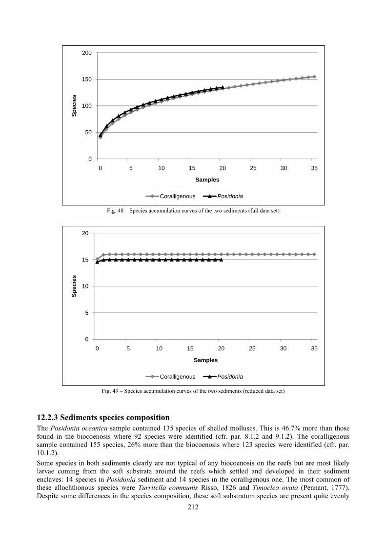
212

Fig. 48 – Species accumulation curves of the two sediments (full data set)

Fig. 49 – Species accumulation curves of the two sediments (reduced data set)

12.2.3 Sediments species composition The Posidonia oceanica sample contained 135 species of shelled molluscs. This is 46.7% more than those found in the biocoenosis where 92 species were identified (cfr. par. 8.1.2 and 9.1.2). The coralligenous sample contained 155 species, 26% more than the biocoenosis where 123 species were identified (cfr. par. 10.1.2). Some species in both sediments clearly are not typical of any biocoenosis on the reefs but are most likely larvae coming from the soft substrata around the reefs which settled and developed in their sediment enclaves: 14 species in Posidonia sediment and 14 species in the coralligenous one. The most common of these allochthonous species were Turritella communis Risso, 1826 and Timoclea ovata (Pennant, 1777). Despite some differences in the species composition, these soft substratum species are present quite evenly

0

50

100

150

200

0 5 10 15 20 25 30 35

Spec

ies

Samples

Coralligenous Posidonia

0

5

10

15

20

0 5 10 15 20 25 30 35

Spec

ies

Samples

Coralligenous Posidonia

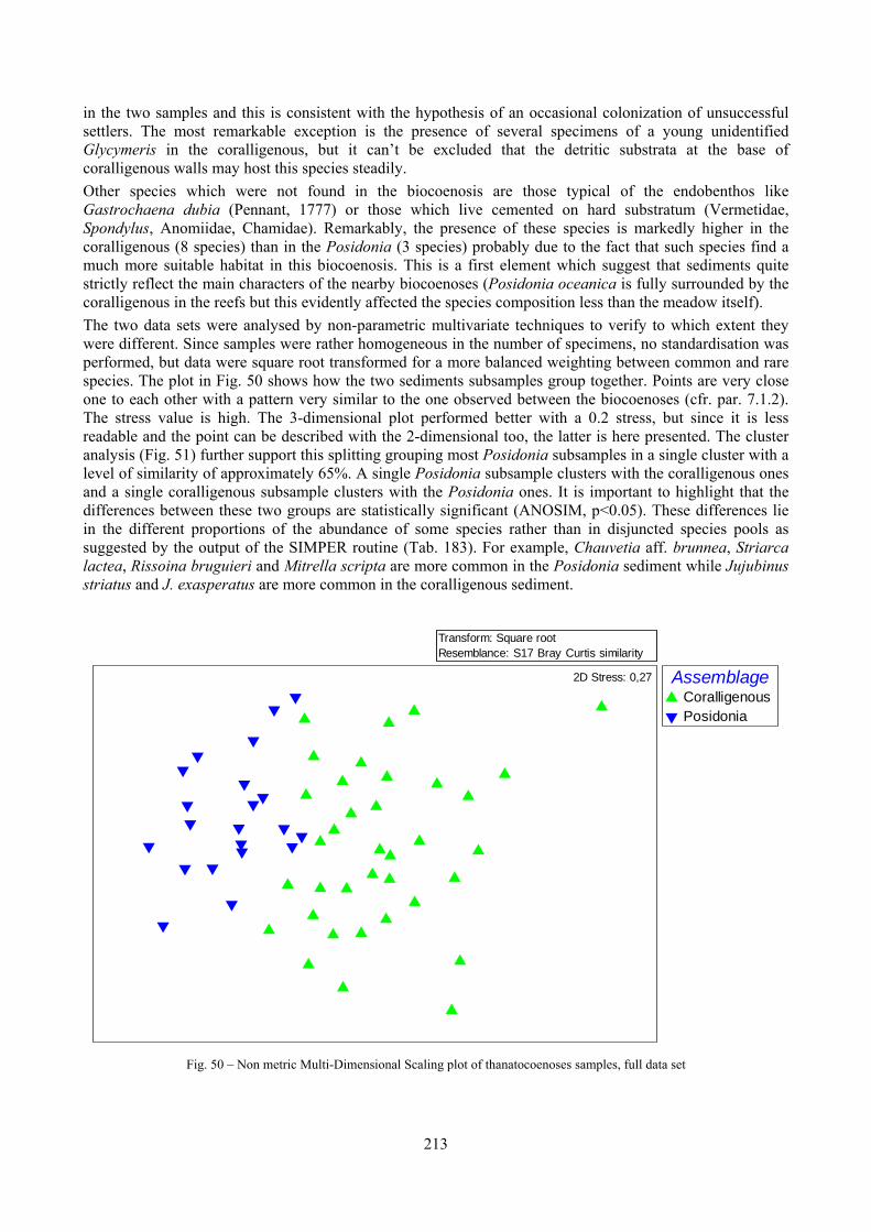
213

in the two samples and this is consistent with the hypothesis of an occasional colonization of unsuccessful settlers. The most remarkable exception is the presence of several specimens of a young unidentified Glycymeris in the coralligenous, but it can’t be excluded that the detritic substrata at the base of coralligenous walls may host this species steadily. Other species which were not found in the biocoenosis are those typical of the endobenthos like Gastrochaena dubia (Pennant, 1777) or those which live cemented on hard substratum (Vermetidae, Spondylus, Anomiidae, Chamidae). Remarkably, the presence of these species is markedly higher in the coralligenous (8 species) than in the Posidonia (3 species) probably due to the fact that such species find a much more suitable habitat in this biocoenosis. This is a first element which suggest that sediments quite strictly reflect the main characters of the nearby biocoenoses (Posidonia oceanica is fully surrounded by the coralligenous in the reefs but this evidently affected the species composition less than the meadow itself). The two data sets were analysed by non-parametric multivariate techniques to verify to which extent they were different. Since samples were rather homogeneous in the number of specimens, no standardisation was performed, but data were square root transformed for a more balanced weighting between common and rare species. The plot in Fig. 50 shows how the two sediments subsamples group together. Points are very close one to each other with a pattern very similar to the one observed between the biocoenoses (cfr. par. 7.1.2). The stress value is high. The 3-dimensional plot performed better with a 0.2 stress, but since it is less readable and the point can be described with the 2-dimensional too, the latter is here presented. The cluster analysis (Fig. 51) further support this splitting grouping most Posidonia subsamples in a single cluster with a level of similarity of approximately 65%. A single Posidonia subsample clusters with the coralligenous ones and a single coralligenous subsample clusters with the Posidonia ones. It is important to highlight that the differences between these two groups are statistically significant (ANOSIM, p<0.05). These differences lie in the different proportions of the abundance of some species rather than in disjuncted species pools as suggested by the output of the SIMPER routine (Tab. 183). For example, Chauvetia aff. brunnea, Striarca lactea, Rissoina bruguieri and Mitrella scripta are more common in the Posidonia sediment while Jujubinus striatus and J. exasperatus are more common in the coralligenous sediment.

Fig. 50 – Non metric Multi-Dimensional Scaling plot of thanatocoenoses samples, full data set

Transform: Square rootResemblance: S17 Bray Curtis similarity

AssemblageCoralligenousPosidonia

2D Stress: 0,27

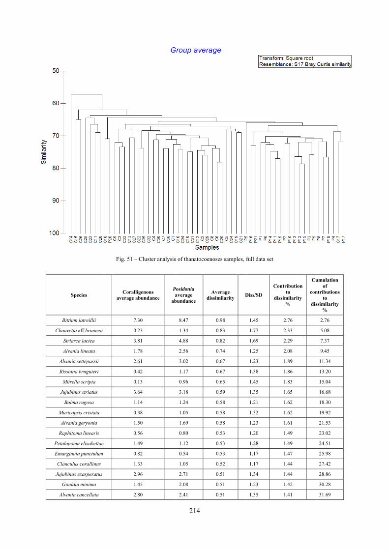
Bitti

Chauve

Stri

Alva

Alvan

Risso

Mitr

Jujub

Bol

Muric

Alva

Raphi

Petalop

Emargi

Clancu

Jujubin

Gou

Alvan

Species

ium latreillii

etia aff brunnea

iarca lactea

ania lineata

nia settepassii

oina bruguieri

rella scripta

binus striatus

lma rugosa

copsis cristata

nia geryonia

itoma linearis

poma elisabettae

inula punctulum

ulus corallinus

nus exasperatus

uldia minima

nia cancellata

Fig. 51 – C

Coralligaverage ab

7.30

0.23

3.8

1.78

2.6

0.42

0.13

3.64

1.14

0.38

1.50

0.56

1.49

0.82

1.33

2.96

1.45

2.80

Cluster analysis

genous undance

Pa

ab

0

3

1

8

1

2

3

4

4

8

0

6

9

2

3

6

5

0

214

s of thanatocoen

Posidonia average bundance di

8.47

1.34

4.88

2.56

3.02

1.17

0.96

3.18

1.24

1.05

1.69

0.80

1.12

0.54

1.05

2.71

2.08

2.41

noses samples, f

Average ssimilarity D

0.98

0.83

0.82

0.74

0.67

0.67

0.65

0.59

0.58

0.58

0.58

0.53

0.53

0.53

0.52

0.51

0.51

0.51

full data set

Diss/SD

Con

diss

1.45

1.77

1.69

1.25

1.23

1.38

1.45

1.35

1.21

1.32

1.23

1.20

1.28

1.17

1.17

1.34

1.23

1.35

ntribution to

similarity %

Cu

con

dis

2.76

2.33

2.29

2.08

1.89

1.86

1.83

1.65

1.62

1.62

1.61

1.49

1.49

1.47

1.44

1.44

1.42

1.41

umulation of

ntributions to

ssimilarity %

2.76

5.08

7.37

9.45

11.34

13.20

15.04

16.68

18.30

19.92

21.53

23.02

24.51

25.98

27.42

28.86

30.28

31.69

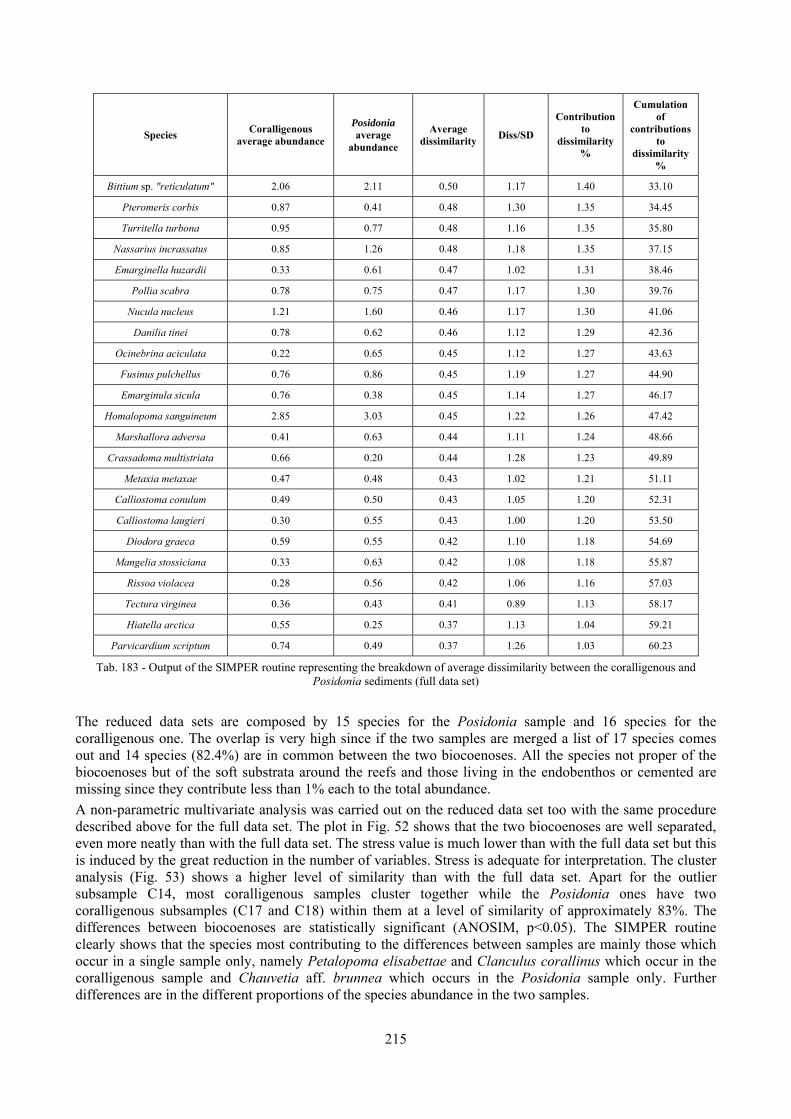
215

Species Coralligenous average abundance

Posidonia average

abundance

Average dissimilarity Diss/SD

Contribution to

dissimilarity %

Cumulation of

contributions to

dissimilarity %

Bittium sp. "reticulatum" 2.06 2.11 0.50 1.17 1.40 33.10

Pteromeris corbis 0.87 0.41 0.48 1.30 1.35 34.45

Turritella turbona 0.95 0.77 0.48 1.16 1.35 35.80

Nassarius incrassatus 0.85 1.26 0.48 1.18 1.35 37.15

Emarginella huzardii 0.33 0.61 0.47 1.02 1.31 38.46

Pollia scabra 0.78 0.75 0.47 1.17 1.30 39.76

Nucula nucleus 1.21 1.60 0.46 1.17 1.30 41.06

Danilia tinei 0.78 0.62 0.46 1.12 1.29 42.36

Ocinebrina aciculata 0.22 0.65 0.45 1.12 1.27 43.63

Fusinus pulchellus 0.76 0.86 0.45 1.19 1.27 44.90

Emarginula sicula 0.76 0.38 0.45 1.14 1.27 46.17

Homalopoma sanguineum 2.85 3.03 0.45 1.22 1.26 47.42

Marshallora adversa 0.41 0.63 0.44 1.11 1.24 48.66

Crassadoma multistriata 0.66 0.20 0.44 1.28 1.23 49.89

Metaxia metaxae 0.47 0.48 0.43 1.02 1.21 51.11

Calliostoma conulum 0.49 0.50 0.43 1.05 1.20 52.31

Calliostoma laugieri 0.30 0.55 0.43 1.00 1.20 53.50

Diodora graeca 0.59 0.55 0.42 1.10 1.18 54.69

Mangelia stossiciana 0.33 0.63 0.42 1.08 1.18 55.87

Rissoa violacea 0.28 0.56 0.42 1.06 1.16 57.03

Tectura virginea 0.36 0.43 0.41 0.89 1.13 58.17

Hiatella arctica 0.55 0.25 0.37 1.13 1.04 59.21

Parvicardium scriptum 0.74 0.49 0.37 1.26 1.03 60.23

Tab. 183 - Output of the SIMPER routine representing the breakdown of average dissimilarity between the coralligenous and Posidonia sediments (full data set)

The reduced data sets are composed by 15 species for the Posidonia sample and 16 species for the coralligenous one. The overlap is very high since if the two samples are merged a list of 17 species comes out and 14 species (82.4%) are in common between the two biocoenoses. All the species not proper of the biocoenoses but of the soft substrata around the reefs and those living in the endobenthos or cemented are missing since they contribute less than 1% each to the total abundance. A non-parametric multivariate analysis was carried out on the reduced data set too with the same procedure described above for the full data set. The plot in Fig. 52 shows that the two biocoenoses are well separated, even more neatly than with the full data set. The stress value is much lower than with the full data set but this is induced by the great reduction in the number of variables. Stress is adequate for interpretation. The cluster analysis (Fig. 53) shows a higher level of similarity than with the full data set. Apart for the outlier subsample C14, most coralligenous samples cluster together while the Posidonia ones have two coralligenous subsamples (C17 and C18) within them at a level of similarity of approximately 83%. The differences between biocoenoses are statistically significant (ANOSIM, p<0.05). The SIMPER routine clearly shows that the species most contributing to the differences between samples are mainly those which occur in a single sample only, namely Petalopoma elisabettae and Clanculus corallinus which occur in the coralligenous sample and Chauvetia aff. brunnea which occurs in the Posidonia sample only. Further differences are in the different proportions of the species abundance in the two samples.

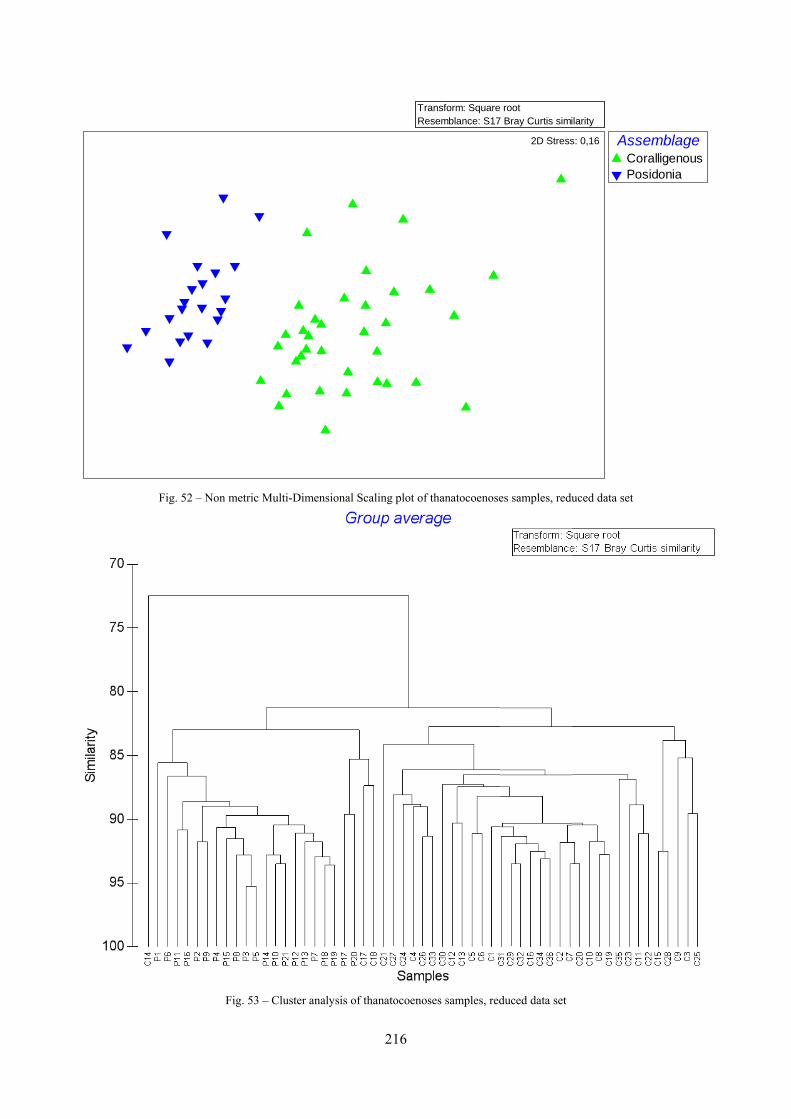
Fig. 52 – Noon metric Multi

Fig. 53 – Clu

i-Dimensional S

uster analysis of

216

Scaling plot of

f thanatocoenos

TraRe

thanatocoenose

ses samples, red

ansform: Square esemblance: S17

es samples, redu

duced data set

root7 Bray Curtis simi

2D Stress

uced data set

ilarity

AsseCoPos

s: 0,16 emblageralligenoussidonia

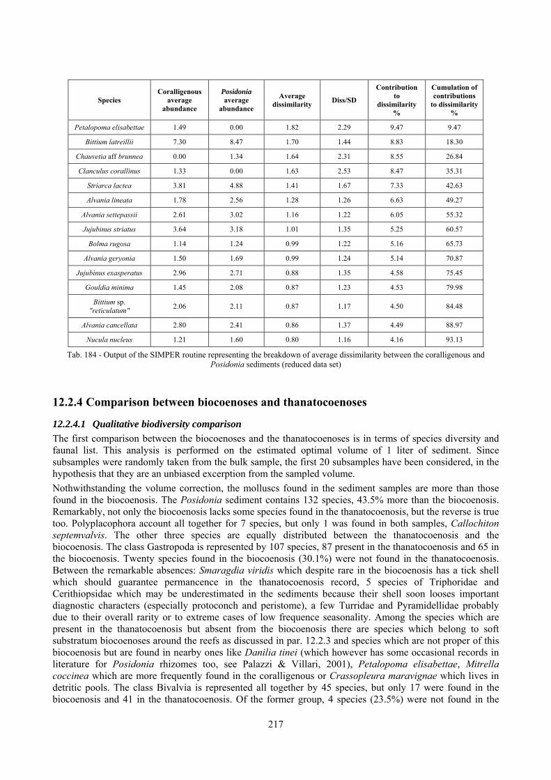
217

Species Coralligenous

average abundance

Posidonia average

abundance

Average dissimilarity Diss/SD

Contribution to

dissimilarity %

Cumulation of contributions

to dissimilarity %

Petalopoma elisabettae 1.49 0.00 1.82 2.29 9.47 9.47

Bittium latreillii 7.30 8.47 1.70 1.44 8.83 18.30

Chauvetia aff brunnea 0.00 1.34 1.64 2.31 8.55 26.84

Clanculus corallinus 1.33 0.00 1.63 2.53 8.47 35.31

Striarca lactea 3.81 4.88 1.41 1.67 7.33 42.63

Alvania lineata 1.78 2.56 1.28 1.26 6.63 49.27

Alvania settepassii 2.61 3.02 1.16 1.22 6.05 55.32

Jujubinus striatus 3.64 3.18 1.01 1.35 5.25 60.57

Bolma rugosa 1.14 1.24 0.99 1.22 5.16 65.73

Alvania geryonia 1.50 1.69 0.99 1.24 5.14 70.87

Jujubinus exasperatus 2.96 2.71 0.88 1.35 4.58 75.45

Gouldia minima 1.45 2.08 0.87 1.23 4.53 79.98

Bittium sp. "reticulatum" 2.06 2.11 0.87 1.17 4.50 84.48

Alvania cancellata 2.80 2.41 0.86 1.37 4.49 88.97

Nucula nucleus 1.21 1.60 0.80 1.16 4.16 93.13

Tab. 184 - Output of the SIMPER routine representing the breakdown of average dissimilarity between the coralligenous and Posidonia sediments (reduced data set)

12.2.4 Comparison between biocoenoses and thanatocoenoses

12.2.4.1 Qualitative biodiversity comparison The first comparison between the biocoenoses and the thanatocoenoses is in terms of species diversity and faunal list. This analysis is performed on the estimated optimal volume of 1 liter of sediment. Since subsamples were randomly taken from the bulk sample, the first 20 subsamples have been considered, in the hypothesis that they are an unbiased excerption from the sampled volume. Nothwithstanding the volume correction, the molluscs found in the sediment samples are more than those found in the biocoenosis. The Posidonia sediment contains 132 species, 43.5% more than the biocoenosis. Remarkably, not only the biocoenosis lacks some species found in the thanatocoenosis, but the reverse is true too. Polyplacophora account all together for 7 species, but only 1 was found in both samples, Callochiton septemvalvis. The other three species are equally distributed between the thanatocoenosis and the biocoenosis. The class Gastropoda is represented by 107 species, 87 present in the thanatocoenosis and 65 in the biocoenosis. Twenty species found in the biocoenosis (30.1%) were not found in the thanatocoenosis. Between the remarkable absences: Smaragdia viridis which despite rare in the biocoenosis has a tick shell which should guarantee permancence in the thanatocoenosis record, 5 species of Triphoridae and Cerithiopsidae which may be underestimated in the sediments because their shell soon looses important diagnostic characters (especially protoconch and peristome), a few Turridae and Pyramidellidae probably due to their overall rarity or to extreme cases of low frequence seasonality. Among the species which are present in the thanatocoenosis but absent from the biocoenosis there are species which belong to soft substratum biocoenoses around the reefs as discussed in par. 12.2.3 and species which are not proper of this biocoenosis but are found in nearby ones like Danilia tinei (which however has some occasional records in literature for Posidonia rhizomes too, see Palazzi & Villari, 2001), Petalopoma elisabettae, Mitrella coccinea which are more frequently found in the coralligenous or Crassopleura maravignae which lives in detritic pools. The class Bivalvia is represented all together by 45 species, but only 17 were found in the biocoenosis and 41 in the thanatocoenosis. Of the former group, 4 species (23.5%) were not found in the

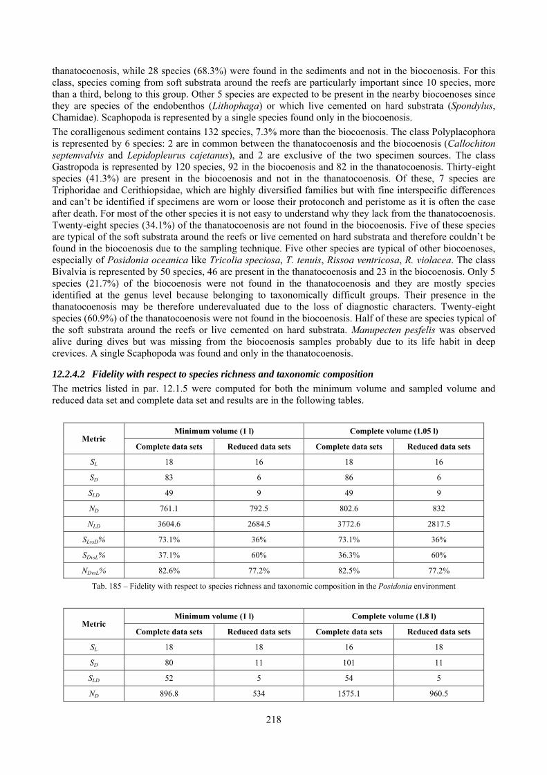
218

thanatocoenosis, while 28 species (68.3%) were found in the sediments and not in the biocoenosis. For this class, species coming from soft substrata around the reefs are particularly important since 10 species, more than a third, belong to this group. Other 5 species are expected to be present in the nearby biocoenoses since they are species of the endobenthos (Lithophaga) or which live cemented on hard substrata (Spondylus, Chamidae). Scaphopoda is represented by a single species found only in the biocoenosis. The coralligenous sediment contains 132 species, 7.3% more than the biocoenosis. The class Polyplacophora is represented by 6 species: 2 are in common between the thanatocoenosis and the biocoenosis (Callochiton septemvalvis and Lepidopleurus cajetanus), and 2 are exclusive of the two specimen sources. The class Gastropoda is represented by 120 species, 92 in the biocoenosis and 82 in the thanatocoenosis. Thirty-eight species (41.3%) are present in the biocoenosis and not in the thanatocoenosis. Of these, 7 species are Triphoridae and Cerithiopsidae, which are highly diversified families but with fine interspecific differences and can’t be identified if specimens are worn or loose their protoconch and peristome as it is often the case after death. For most of the other species it is not easy to understand why they lack from the thanatocoenosis. Twenty-eight species (34.1%) of the thanatocoenosis are not found in the biocoenosis. Five of these species are typical of the soft substrata around the reefs or live cemented on hard substrata and therefore couldn’t be found in the biocoenosis due to the sampling technique. Five other species are typical of other biocoenoses, especially of Posidonia oceanica like Tricolia speciosa, T. tenuis, Rissoa ventricosa, R. violacea. The class Bivalvia is represented by 50 species, 46 are present in the thanatocoenosis and 23 in the biocoenosis. Only 5 species (21.7%) of the biocoenosis were not found in the thanatocoenosis and they are mostly species identified at the genus level because belonging to taxonomically difficult groups. Their presence in the thanatocoenosis may be therefore underevaluated due to the loss of diagnostic characters. Twenty-eight species (60.9%) of the thanatocoenosis were not found in the biocoenosis. Half of these are species typical of the soft substrata around the reefs or live cemented on hard substrata. Manupecten pesfelis was observed alive during dives but was missing from the biocoenosis samples probably due to its life habit in deep crevices. A single Scaphopoda was found and only in the thanatocoenosis.

12.2.4.2 Fidelity with respect to species richness and taxonomic composition The metrics listed in par. 12.1.5 were computed for both the minimum volume and sampled volume and reduced data set and complete data set and results are in the following tables.

Metric Minimum volume (1 l) Complete volume (1.05 l)

Complete data sets Reduced data sets Complete data sets Reduced data sets

SL 18 16 18 16

SD 83 6 86 6

SLD 49 9 49 9

ND 761.1 792.5 802.6 832

NLD 3604.6 2684.5 3772.6 2817.5

SLvsD% 73.1% 36% 73.1% 36%

SDvsL% 37.1% 60% 36.3% 60%

NDvsL% 82.6% 77.2% 82.5% 77.2%

Tab. 185 – Fidelity with respect to species richness and taxonomic composition in the Posidonia environment

Metric Minimum volume (1 l) Complete volume (1.8 l)

Complete data sets Reduced data sets Complete data sets Reduced data sets

SL 18 18 16 18

SD 80 11 101 11

SLD 52 5 54 5

ND 896.8 534 1575.1 960.5

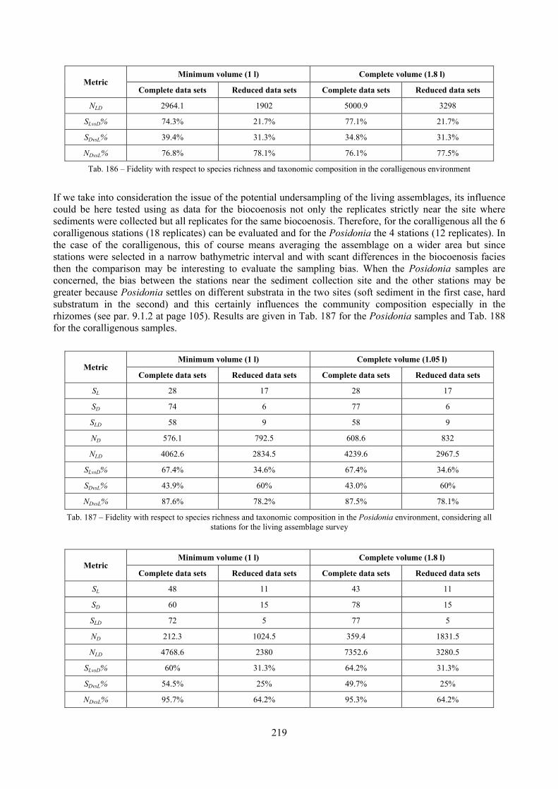
219

Metric Minimum volume (1 l) Complete volume (1.8 l)

Complete data sets Reduced data sets Complete data sets Reduced data sets

NLD 2964.1 1902 5000.9 3298

SLvsD% 74.3% 21.7% 77.1% 21.7%

SDvsL% 39.4% 31.3% 34.8% 31.3%

NDvsL% 76.8% 78.1% 76.1% 77.5%

Tab. 186 – Fidelity with respect to species richness and taxonomic composition in the coralligenous environment

If we take into consideration the issue of the potential undersampling of the living assemblages, its influence could be here tested using as data for the biocoenosis not only the replicates strictly near the site where sediments were collected but all replicates for the same biocoenosis. Therefore, for the coralligenous all the 6 coralligenous stations (18 replicates) can be evaluated and for the Posidonia the 4 stations (12 replicates). In the case of the coralligenous, this of course means averaging the assemblage on a wider area but since stations were selected in a narrow bathymetric interval and with scant differences in the biocoenosis facies then the comparison may be interesting to evaluate the sampling bias. When the Posidonia samples are concerned, the bias between the stations near the sediment collection site and the other stations may be greater because Posidonia settles on different substrata in the two sites (soft sediment in the first case, hard substratum in the second) and this certainly influences the community composition especially in the rhizomes (see par. 9.1.2 at page 105). Results are given in Tab. 187 for the Posidonia samples and Tab. 188 for the coralligenous samples.

Metric Minimum volume (1 l) Complete volume (1.05 l)

Complete data sets Reduced data sets Complete data sets Reduced data sets

SL 28 17 28 17

SD 74 6 77 6

SLD 58 9 58 9

ND 576.1 792.5 608.6 832

NLD 4062.6 2834.5 4239.6 2967.5

SLvsD% 67.4% 34.6% 67.4% 34.6%

SDvsL% 43.9% 60% 43.0% 60%

NDvsL% 87.6% 78.2% 87.5% 78.1%

Tab. 187 – Fidelity with respect to species richness and taxonomic composition in the Posidonia environment, considering all stations for the living assemblage survey

Metric Minimum volume (1 l) Complete volume (1.8 l)

Complete data sets Reduced data sets Complete data sets Reduced data sets

SL 48 11 43 11

SD 60 15 78 15

SLD 72 5 77 5

ND 212.3 1024.5 359.4 1831.5

NLD 4768.6 2380 7352.6 3280.5

SLvsD% 60% 31.3% 64.2% 31.3%

SDvsL% 54.5% 25% 49.7% 25%

NDvsL% 95.7% 64.2% 95.3% 64.2%

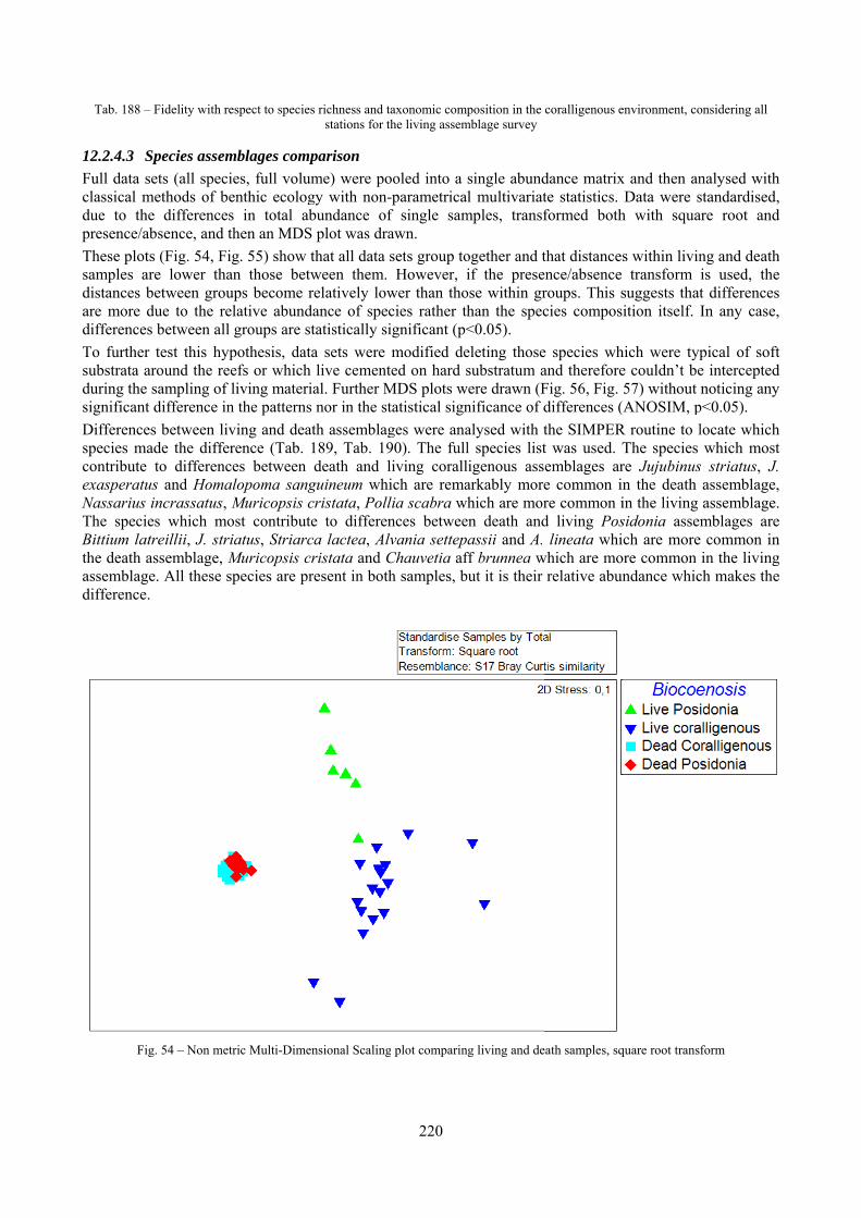
Tab. 188 – F

12.2.4.3 SpFull data seclassical medue to the presence/abThese plots samples aredistances beare more dudifferences To further substrata arduring the ssignificant dDifferencesspecies madcontribute texasperatusNassarius inThe speciesBittium latrthe death asassemblagedifference.

Fig.

Fidelity with re

pecies assemets (all specieethods of be

differencesbsence, and th

(Fig. 54, Fige lower thanetween grouue to the relbetween all test this hyp

round the reesampling of ldifference ins between livde the differto differences and Homalncrassatus, Ms which moreillii, J. strissemblage, M. All these sp

. 54 – Non metr

espect to species

mblages compes, full volum

enthic ecologs in total abhen an MDSg. 55) show tn those betw

ups become rlative abundgroups are st

pothesis, datefs or which living materi

n the patternsving and dearence (Tab. es between lopoma sangMuricopsis c

ost contributeiatus, StriarcMuricopsis cpecies are pr

ric Multi-Dime

s richness and tstations for t

parison me) were pogy with non-bundance of

S plot was drathat all data ween them.relatively lowdance of spectatistically sia sets were live cement

ial. Further Ms nor in the stath assemblag189, Tab. 19death and l

guineum whicristata, Polle to differenca lactea, Alristata and Cresent in both

nsional Scaling

220

taxonomic compthe living assem

ooled into a -parametricaf single samawn. sets group toHowever, i

wer than thocies rather thignificant (p<modified de

ted on hard sMDS plots wtatistical signges were ana90). The fullliving corallich are remalia scabra wnces betweelvania settepChauvetia afh samples, b

g plot comparin

position in the mblage survey

single abundl multivariat

mples, transf

ogether and tif the prese

ose within grhan the spec<0.05). eleting thosesubstratum a

were drawn (Fnificance of dalysed with tl species listligenous assarkably more

which are moren death andassii and A.

ff brunnea wbut it is their

ng living and de

coralligenous e

dance matrixte statistics. formed both

that distancesnce/absence roups. This scies compos

e species whand thereforeFig. 56, Fig. differences (the SIMPERt was used. Temblages are common inre common id living Pos

lineata whiwhich are mo

relative abun

ath samples, sq

environment, co

x and then anData were s

h with squa

s within livintransform

suggests thatition itself. I

hich were type couldn’t be57) without

(ANOSIM, pR routine to lThe species re Jujubinusn the death in the living sidonia assemch are more

ore common ndance whic

quare root transf

onsidering all

nalysed withstandardised,are root and

ng and deathis used, thet differencesIn any case,

pical of softe interceptednoticing any

p<0.05). locate whichwhich most

s striatus, J.assemblage,assemblage.mblages are common inin the living

ch makes the

form

h ,

d

h e s ,

t d y

h t

, . e n g e

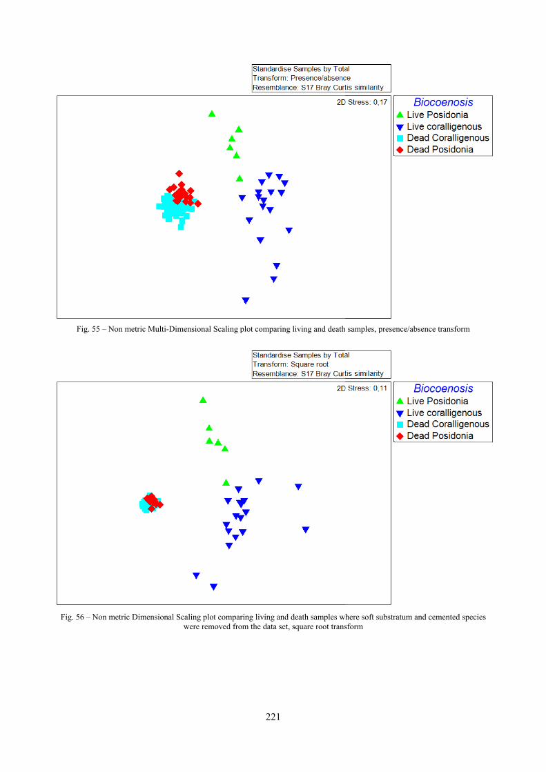
Fig. 55

Fig. 56 – No

5 – Non metric M

on metric Dime

Multi-Dimensio

ensional Scalingwere

onal Scaling pl

g plot comparine removed from

221

ot comparing li

ng living and dem the data set, sq

iving and death

eath samples whquare root trans

h samples, prese

here soft substrsform

ence/absence tra

ratum and ceme

ansform

ented species

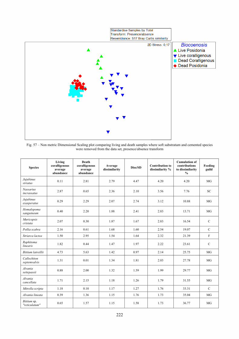
Fig. 57 – No

Species

Jujubinus striatus

Nassarius incrassatus

Jujubinus exasperatus

Homalopoma sanguineum

Muricopsis cristata

Pollia scabra

Striarca lactea

Raphitoma linearis

Bittium latreillii

Callochiton septemvalvis

Alvania settepassii

Alvania cancellata

Mitrella scripta

Alvania lineata

Bittium sp. "reticulatum"

on metric Dime

Living coralligeno

averageabundan

0.11

2.87

0.29

0.40

2.07

2.16

1.50

1.82

i 4.73

1.31

0.88

1.71

1.18

0.39

0.65

ensional Scalingwere re

ous e ce

Deacorallig

averabund

2.8

0.6

2.2

2.2

0.3

0.6

2.9

0.4

5.6

0.0

2.0

2.1

0.1

1.3

1.5

g plot comparinemoved from th

ath genous rage dance

Adiss

81

65

29

20

30

61

95

44

63

01

00

15

10

36

57

222

ng living and dehe data set, prese

Average similarity

2.79

2.36

2.07

1.88

1.87

1.68

1.54

1.47

1.42

1.34

1.32

1.18

1.17

1.15

1.15

eath samples whence/absence tr

Diss/SD Cd

4.47

2.10

2.74

2.41

1.67

1.60

1.64

1.97

0.97

1.81

1.59

1.26

1.27

1.76

1.58

here soft substrransform

Contribution to dissimilarity %

4.20

3.56

3.12

2.83

2.83

2.54

2.32

2.22

2.14

2.03

1.99

1.79

1.76

1.73

1.73

ratum and ceme

Cumulation ocontribution

to dissimilarit%

4.20

7.76

10.88

13.71

16.54

19.07

21.39

23.61

25.75

27.78

29.77

31.55

33.31

35.04

36.77

ented species

of s ty

Feeding guild

MG

SC

MG

MG

C

C

F

C

MG

MG

MG

MG

C

MG

MG

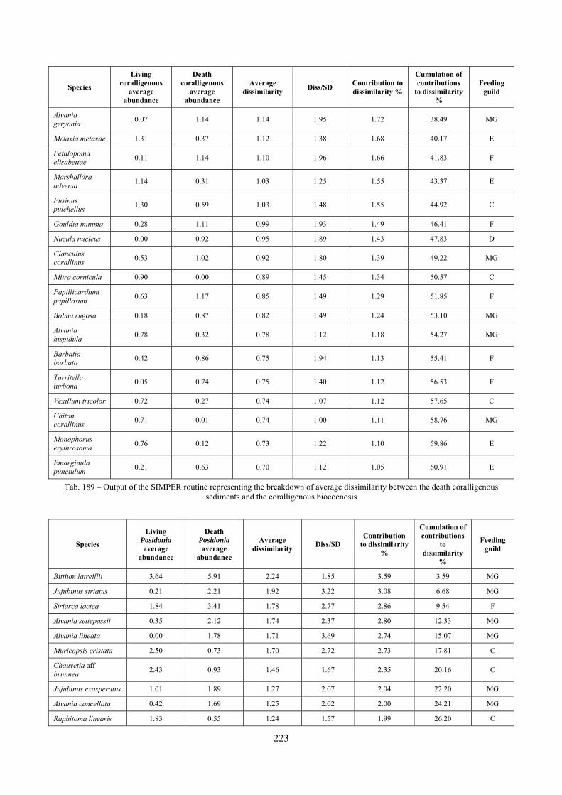
223

Species

Living coralligenous

average abundance

Death coralligenous

average abundance

Average dissimilarity Diss/SD Contribution to

dissimilarity %

Cumulation of contributions

to dissimilarity %

Feeding guild

Alvania geryonia 0.07 1.14 1.14 1.95 1.72 38.49 MG

Metaxia metaxae 1.31 0.37 1.12 1.38 1.68 40.17 E

Petalopoma elisabettae 0.11 1.14 1.10 1.96 1.66 41.83 F

Marshallora adversa 1.14 0.31 1.03 1.25 1.55 43.37 E

Fusinus pulchellus 1.30 0.59 1.03 1.48 1.55 44.92 C

Gouldia minima 0.28 1.11 0.99 1.93 1.49 46.41 F

Nucula nucleus 0.00 0.92 0.95 1.89 1.43 47.83 D

Clanculus corallinus 0.53 1.02 0.92 1.80 1.39 49.22 MG

Mitra cornicula 0.90 0.00 0.89 1.45 1.34 50.57 C

Papillicardium papillosum 0.63 1.17 0.85 1.49 1.29 51.85 F

Bolma rugosa 0.18 0.87 0.82 1.49 1.24 53.10 MG

Alvania hispidula 0.78 0.32 0.78 1.12 1.18 54.27 MG

Barbatia barbata 0.42 0.86 0.75 1.94 1.13 55.41 F

Turritella turbona 0.05 0.74 0.75 1.40 1.12 56.53 F

Vexillum tricolor 0.72 0.27 0.74 1.07 1.12 57.65 C

Chiton corallinus 0.71 0.01 0.74 1.00 1.11 58.76 MG

Monophorus erythrosoma 0.76 0.12 0.73 1.22 1.10 59.86 E

Emarginula punctulum 0.21 0.63 0.70 1.12 1.05 60.91 E

Tab. 189 – Output of the SIMPER routine representing the breakdown of average dissimilarity between the death coralligenous sediments and the coralligenous biocoenosis

Species

Living Posidonia average

abundance

Death Posidonia average

abundance

Average dissimilarity Diss/SD

Contribution to dissimilarity

%

Cumulation of contributions

to dissimilarity

%

Feeding guild

Bittium latreillii 3.64 5.91 2.24 1.85 3.59 3.59 MG

Jujubinus striatus 0.21 2.21 1.92 3.22 3.08 6.68 MG

Striarca lactea 1.84 3.41 1.78 2.77 2.86 9.54 F

Alvania settepassii 0.35 2.12 1.74 2.37 2.80 12.33 MG

Alvania lineata 0.00 1.78 1.71 3.69 2.74 15.07 MG

Muricopsis cristata 2.50 0.73 1.70 2.72 2.73 17.81 C

Chauvetia aff brunnea 2.43 0.93 1.46 1.67 2.35 20.16 C

Jujubinus exasperatus 1.01 1.89 1.27 2.07 2.04 22.20 MG

Alvania cancellata 0.42 1.69 1.25 2.02 2.00 24.21 MG

Raphitoma linearis 1.83 0.55 1.24 1.57 1.99 26.20 C

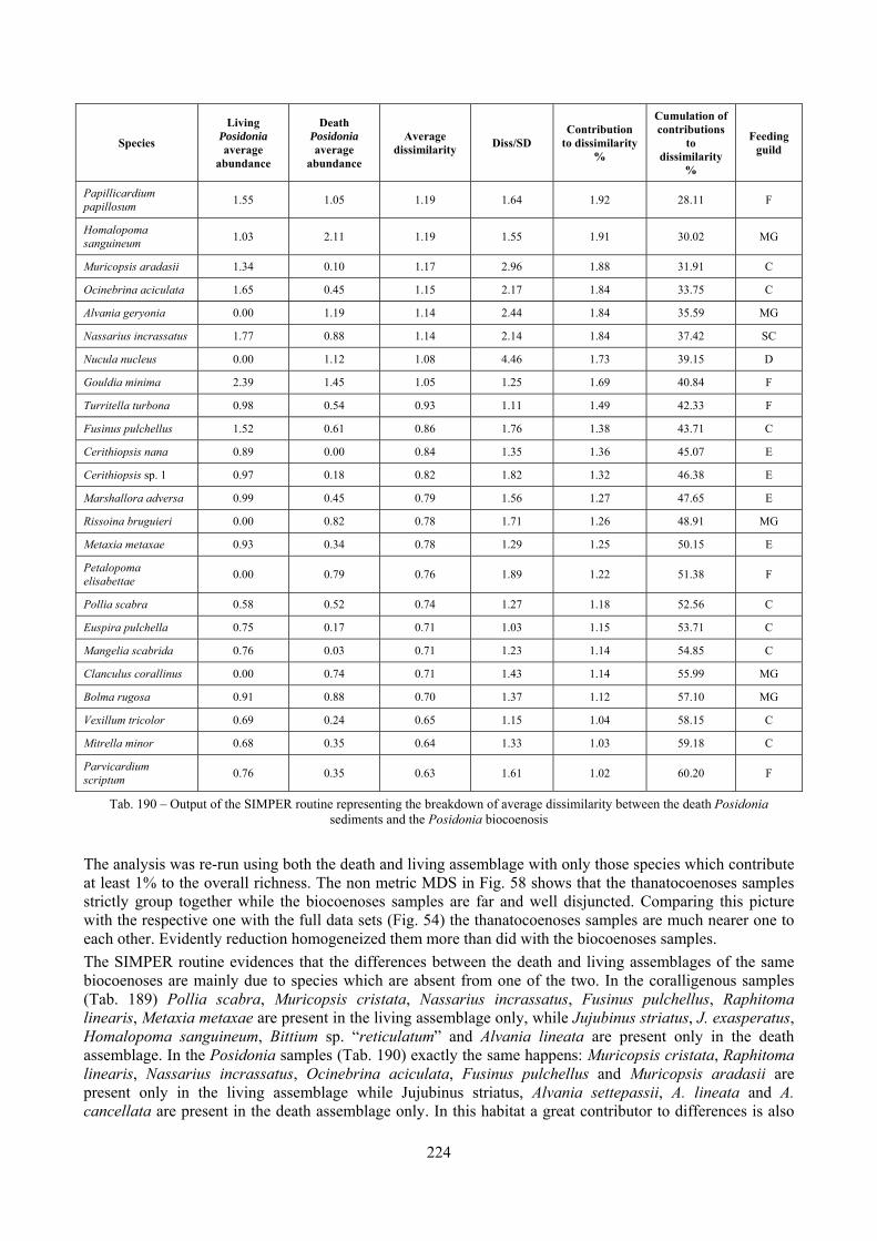
224

Species

Living Posidonia average

abundance

Death Posidonia average

abundance

Average dissimilarity Diss/SD

Contribution to dissimilarity

%

Cumulation of contributions

to dissimilarity

%

Feeding guild

Papillicardium papillosum 1.55 1.05 1.19 1.64 1.92 28.11 F

Homalopoma sanguineum 1.03 2.11 1.19 1.55 1.91 30.02 MG

Muricopsis aradasii 1.34 0.10 1.17 2.96 1.88 31.91 C

Ocinebrina aciculata 1.65 0.45 1.15 2.17 1.84 33.75 C

Alvania geryonia 0.00 1.19 1.14 2.44 1.84 35.59 MG

Nassarius incrassatus 1.77 0.88 1.14 2.14 1.84 37.42 SC

Nucula nucleus 0.00 1.12 1.08 4.46 1.73 39.15 D

Gouldia minima 2.39 1.45 1.05 1.25 1.69 40.84 F

Turritella turbona 0.98 0.54 0.93 1.11 1.49 42.33 F

Fusinus pulchellus 1.52 0.61 0.86 1.76 1.38 43.71 C

Cerithiopsis nana 0.89 0.00 0.84 1.35 1.36 45.07 E

Cerithiopsis sp. 1 0.97 0.18 0.82 1.82 1.32 46.38 E

Marshallora adversa 0.99 0.45 0.79 1.56 1.27 47.65 E

Rissoina bruguieri 0.00 0.82 0.78 1.71 1.26 48.91 MG

Metaxia metaxae 0.93 0.34 0.78 1.29 1.25 50.15 E

Petalopoma elisabettae 0.00 0.79 0.76 1.89 1.22 51.38 F

Pollia scabra 0.58 0.52 0.74 1.27 1.18 52.56 C

Euspira pulchella 0.75 0.17 0.71 1.03 1.15 53.71 C

Mangelia scabrida 0.76 0.03 0.71 1.23 1.14 54.85 C

Clanculus corallinus 0.00 0.74 0.71 1.43 1.14 55.99 MG

Bolma rugosa 0.91 0.88 0.70 1.37 1.12 57.10 MG

Vexillum tricolor 0.69 0.24 0.65 1.15 1.04 58.15 C

Mitrella minor 0.68 0.35 0.64 1.33 1.03 59.18 C

Parvicardium scriptum 0.76 0.35 0.63 1.61 1.02 60.20 F

Tab. 190 – Output of the SIMPER routine representing the breakdown of average dissimilarity between the death Posidonia sediments and the Posidonia biocoenosis

The analysis was re-run using both the death and living assemblage with only those species which contribute at least 1% to the overall richness. The non metric MDS in Fig. 58 shows that the thanatocoenoses samples strictly group together while the biocoenoses samples are far and well disjuncted. Comparing this picture with the respective one with the full data sets (Fig. 54) the thanatocoenoses samples are much nearer one to each other. Evidently reduction homogeneized them more than did with the biocoenoses samples. The SIMPER routine evidences that the differences between the death and living assemblages of the same biocoenoses are mainly due to species which are absent from one of the two. In the coralligenous samples (Tab. 189) Pollia scabra, Muricopsis cristata, Nassarius incrassatus, Fusinus pulchellus, Raphitoma linearis, Metaxia metaxae are present in the living assemblage only, while Jujubinus striatus, J. exasperatus, Homalopoma sanguineum, Bittium sp. “reticulatum” and Alvania lineata are present only in the death assemblage. In the Posidonia samples (Tab. 190) exactly the same happens: Muricopsis cristata, Raphitoma linearis, Nassarius incrassatus, Ocinebrina aciculata, Fusinus pulchellus and Muricopsis aradasii are present only in the living assemblage while Jujubinus striatus, Alvania settepassii, A. lineata and A. cancellata are present in the death assemblage only. In this habitat a great contributor to differences is also

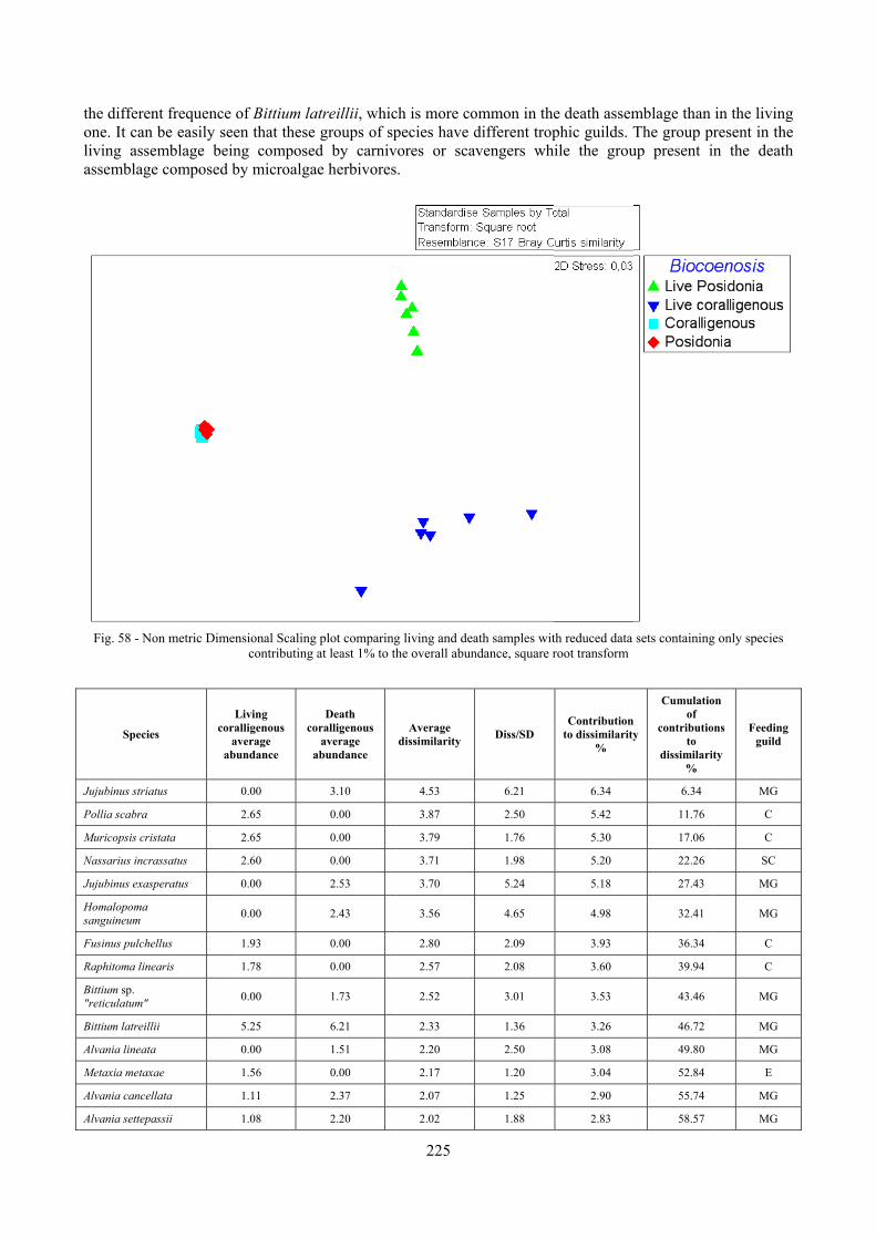
the differenone. It can bliving assemassemblage

Fig. 58 - No

Species

Jujubinus striatu

Pollia scabra

Muricopsis crist

Nassarius incra

Jujubinus exasp

Homalopoma sanguineum

Fusinus pulchel

Raphitoma linea

Bittium sp. "reticulatum"

Bittium latreillii

Alvania lineata

Metaxia metaxa

Alvania cancella

Alvania settepas

nt frequence obe easily seemblage beincomposed b

n metric Dimen

s

Lcora

avabu

us

tata

ssatus

peratus

llus

aris

i

ae

ata

ssii

of Bittium laen that these ng composedby microalga

nsional Scaling contributing

Living alligenous verage undance

co

a

0.00

2.65

2.65

2.60

0.00

0.00

1.93

1.78

0.00

5.25

0.00

1.56

1.11

1.08

atreillii, whicgroups of sp

d by carnivae herbivores

plot comparingat least 1% to th

Death oralligenous

average abundance

3.10

0.00

0.00

0.00

2.53

2.43

0.00

0.00

1.73

6.21

1.51

0.00

2.37

2.20

225

ch is more copecies have d

vores or scas.

g living and deahe overall abun

Average dissimilarity

4.53

3.87

3.79

3.71

3.70

3.56

2.80

2.57

2.52

2.33

2.20

2.17

2.07

2.02

ommon in thedifferent trop

avengers wh

ath samples witndance, square r

Diss/SD

6.21

2.50

1.76

1.98

5.24

4.65

2.09

2.08

3.01

1.36

2.50

1.20

1.25

1.88

e death assemphic guilds. Tile the grou

th reduced data root transform

Contributionto dissimilarity

%

6.34

5.42

5.30

5.20

5.18

4.98

3.93

3.60

3.53

3.26

3.08

3.04

2.90

2.83

mblage than The group pup present i

sets containing

n y

Cumulatioof

contributioto

dissimilari%

6.34

11.76

17.06

22.26

27.43

32.41

36.34

39.94

43.46

46.72

49.80

52.84

55.74

58.57

in the livingresent in the

in the death

g only species

on

ons

ity

Feeding guild

MG

C

C

SC

MG

MG

C

C

MG

MG

MG

E

MG

MG

g e h

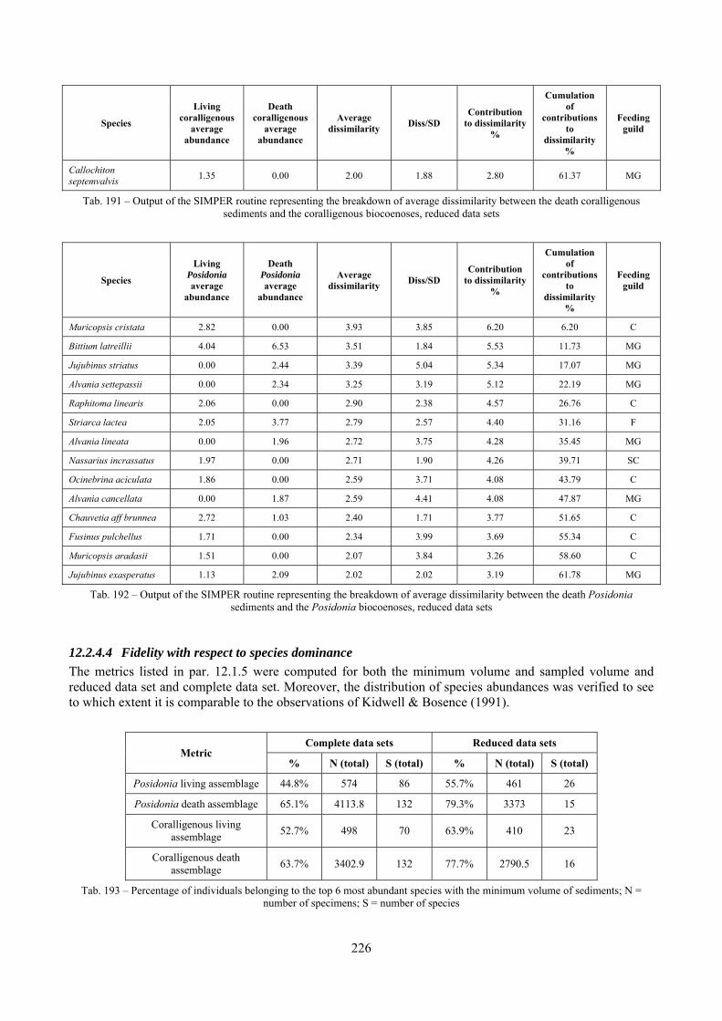
226

Species

Living coralligenous

average abundance

Death coralligenous

average abundance

Average dissimilarity Diss/SD

Contribution to dissimilarity

%

Cumulation of

contributions to

dissimilarity %

Feeding guild

Callochiton septemvalvis 1.35 0.00 2.00 1.88 2.80 61.37 MG

Tab. 191 – Output of the SIMPER routine representing the breakdown of average dissimilarity between the death coralligenous sediments and the coralligenous biocoenoses, reduced data sets

Species

Living Posidonia average

abundance

Death Posidonia average

abundance

Average dissimilarity Diss/SD

Contribution to dissimilarity

%

Cumulation of

contributions to

dissimilarity %

Feeding guild

Muricopsis cristata 2.82 0.00 3.93 3.85 6.20 6.20 C

Bittium latreillii 4.04 6.53 3.51 1.84 5.53 11.73 MG

Jujubinus striatus 0.00 2.44 3.39 5.04 5.34 17.07 MG

Alvania settepassii 0.00 2.34 3.25 3.19 5.12 22.19 MG

Raphitoma linearis 2.06 0.00 2.90 2.38 4.57 26.76 C

Striarca lactea 2.05 3.77 2.79 2.57 4.40 31.16 F

Alvania lineata 0.00 1.96 2.72 3.75 4.28 35.45 MG

Nassarius incrassatus 1.97 0.00 2.71 1.90 4.26 39.71 SC

Ocinebrina aciculata 1.86 0.00 2.59 3.71 4.08 43.79 C

Alvania cancellata 0.00 1.87 2.59 4.41 4.08 47.87 MG

Chauvetia aff brunnea 2.72 1.03 2.40 1.71 3.77 51.65 C

Fusinus pulchellus 1.71 0.00 2.34 3.99 3.69 55.34 C

Muricopsis aradasii 1.51 0.00 2.07 3.84 3.26 58.60 C

Jujubinus exasperatus 1.13 2.09 2.02 2.02 3.19 61.78 MG

Tab. 192 – Output of the SIMPER routine representing the breakdown of average dissimilarity between the death Posidonia sediments and the Posidonia biocoenoses, reduced data sets

12.2.4.4 Fidelity with respect to species dominance The metrics listed in par. 12.1.5 were computed for both the minimum volume and sampled volume and reduced data set and complete data set. Moreover, the distribution of species abundances was verified to see to which extent it is comparable to the observations of Kidwell & Bosence (1991).

Metric Complete data sets Reduced data sets

% N (total) S (total) % N (total) S (total)

Posidonia living assemblage 44.8% 574 86 55.7% 461 26

Posidonia death assemblage 65.1% 4113.8 132 79.3% 3373 15

Coralligenous living assemblage 52.7% 498 70 63.9% 410 23

Coralligenous death assemblage 63.7% 3402.9 132 77.7% 2790.5 16

Tab. 193 – Percentage of individuals belonging to the top 6 most abundant species with the minimum volume of sediments; N = number of specimens; S = number of species

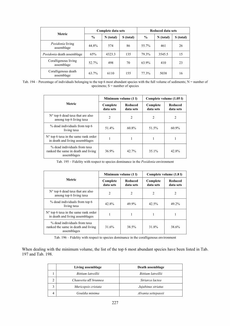
227

Metric Complete data sets Reduced data sets

% N (total) S (total) % N (total) S (total)

Posidonia living assemblage 44.8% 574 86 55.7% 461 26

Posidonia death assemblage 65% 4323.3 135 79.3% 3545.5 15

Coralligenous living assemblage 52.7% 498 70 63.9% 410 23

Coralligenous death assemblage 63.7% 6110 155 77.3% 5038 16

Tab. 194 – Percentage of individuals belonging to the top 6 most abundant species with the full volume of sediments; N = number of specimens; S = number of species

Metric Minimum volume (1 l) Complete volume (1.05 l)

Complete data sets

Reduced data sets

Complete data sets

Reduced data sets

N° top 6 dead taxa that are also among top 6 living taxa 2 2 2 2

% dead individuals from top 6 living taxa 51.4% 60.8% 51.5% 60.9%

N° top 6 taxa in the same rank order in death and living assemblages 1 1 1 1

% dead individuals from taxa ranked the same in death and living

assemblages 36.9% 42.7% 35.1% 42.8%

Tab. 195 – Fidelity with respect to species dominance in the Posidonia environment

Metric Minimum volume (1 l) Complete volume (1.8 l)

Complete data sets

Reduced data sets

Complete data sets

Reduced data sets

N° top 6 dead taxa that are also among top 6 living taxa 2 2 2 2

% dead individuals from top 6 living taxa 42.8% 49.9% 42.5% 49.2%

N° top 6 taxa in the same rank order in death and living assemblages 1 1 1 1

% dead individuals from taxa ranked the same in death and living

assemblages 31.6% 38.5% 31.8% 38.6%

Tab. 196 – Fidelity with respect to species dominance in the coralligenous environment

When dealing with the minimum volume, the list of the top 6 most abundant species have been listed in Tab. 197 and Tab. 198.

Living assemblage Death assemblage

1 Bittium latreillii Bittium latreillii

2 Chauvetia aff brunnea Striarca lactea

3 Muricopsis cristata Jujubinus striatus

4 Gouldia minima Alvania settepassii

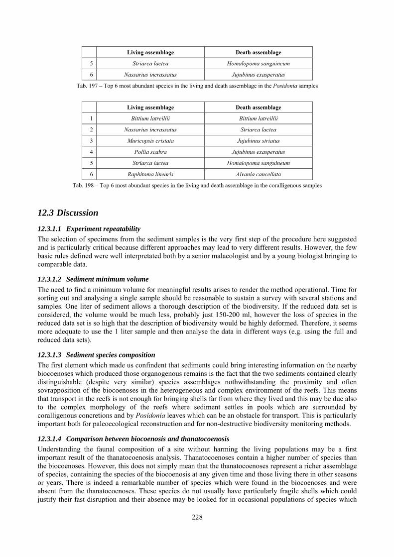
228

Living assemblage Death assemblage

5 Striarca lactea Homalopoma sanguineum

6 Nassarius incrassatus Jujubinus exasperatus

Tab. 197 – Top 6 most abundant species in the living and death assemblage in the Posidonia samples

Living assemblage Death assemblage

1 Bittium latreillii Bittium latreillii

2 Nassarius incrassatus Striarca lactea

3 Muricopsis cristata Jujubinus striatus

4 Pollia scabra Jujubinus exasperatus

5 Striarca lactea Homalopoma sanguineum

6 Raphitoma linearis Alvania cancellata

Tab. 198 – Top 6 most abundant species in the living and death assemblage in the coralligenous samples

12.3 Discussion

12.3.1.1 Experiment repeatability The selection of specimens from the sediment samples is the very first step of the procedure here suggested and is particularly critical because different approaches may lead to very different results. However, the few basic rules defined were well interpretated both by a senior malacologist and by a young biologist bringing to comparable data.

12.3.1.2 Sediment minimum volume The need to find a minimum volume for meaningful results arises to render the method operational. Time for sorting out and analysing a single sample should be reasonable to sustain a survey with several stations and samples. One liter of sediment allows a thorough description of the biodiversity. If the reduced data set is considered, the volume would be much less, probably just 150-200 ml, however the loss of species in the reduced data set is so high that the description of biodiversity would be highly deformed. Therefore, it seems more adequate to use the 1 liter sample and then analyse the data in different ways (e.g. using the full and reduced data sets).

12.3.1.3 Sediment species composition The first element which made us confindent that sediments could bring interesting information on the nearby biocoenoses which produced those organogenous remains is the fact that the two sediments contained clearly distinguishable (despite very similar) species assemblages nothwithstanding the proximity and often sovrapposition of the biocoenoses in the heterogeneous and complex environment of the reefs. This means that transport in the reefs is not enough for bringing shells far from where they lived and this may be due also to the complex morphology of the reefs where sediment settles in pools which are surrounded by coralligenous concretions and by Posidonia leaves which can be an obstacle for transport. This is particularly important both for paleoecological reconstruction and for non-destructive biodiversity monitoring methods.

12.3.1.4 Comparison between biocoenosis and thanatocoenosis Understanding the faunal composition of a site without harming the living populations may be a first important result of the thanatocoenosis analysis. Thanatocoenoses contain a higher number of species than the biocoenoses. However, this does not simply mean that the thanatocoenoses represent a richer assemblage of species, containing the species of the biocoenosis at any given time and those living there in other seasons or years. There is indeed a remarkable number of species which were found in the biocoenoses and were absent from the thanatocoenoses. These species do not usually have particularly fragile shells which could justify their fast disruption and their absence may be looked for in occasional populations of species which

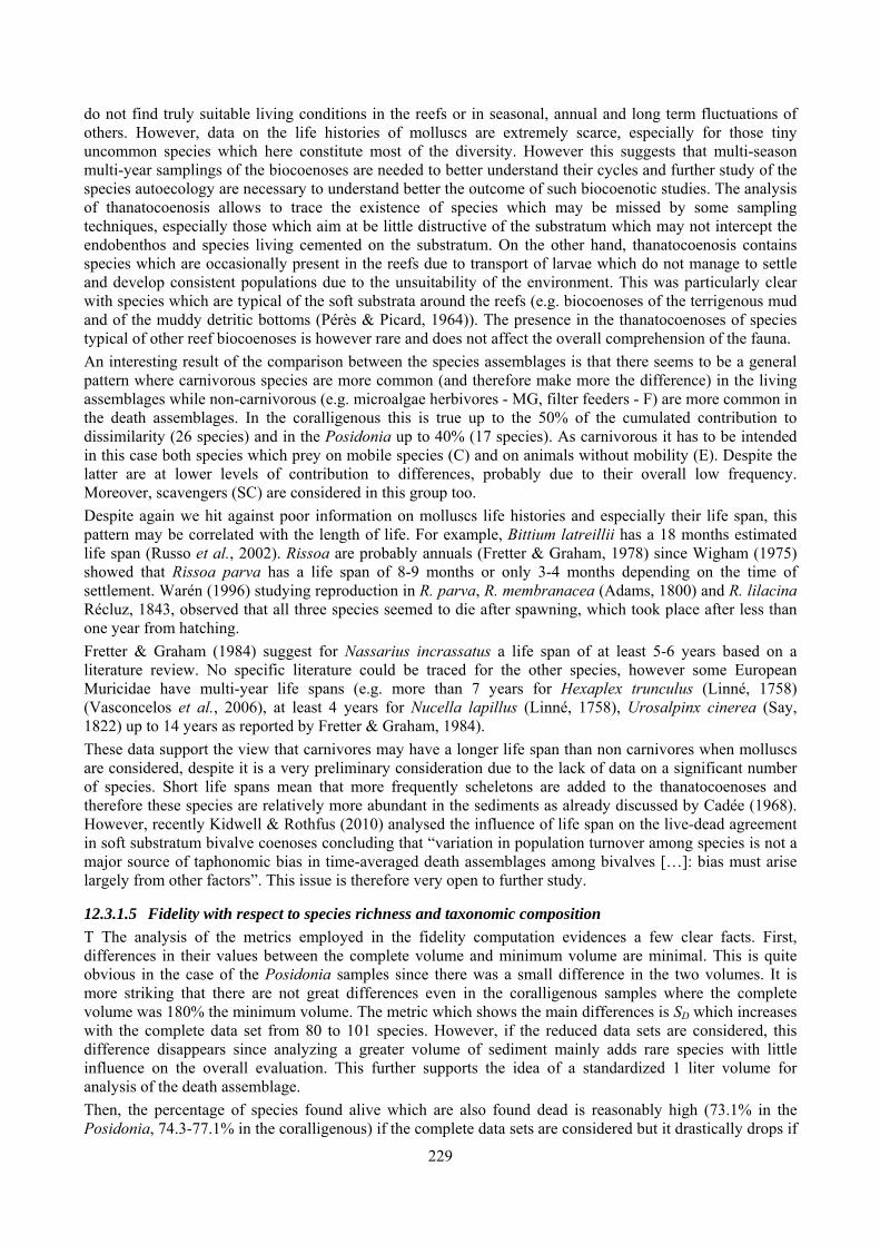
229

do not find truly suitable living conditions in the reefs or in seasonal, annual and long term fluctuations of others. However, data on the life histories of molluscs are extremely scarce, especially for those tiny uncommon species which here constitute most of the diversity. However this suggests that multi-season multi-year samplings of the biocoenoses are needed to better understand their cycles and further study of the species autoecology are necessary to understand better the outcome of such biocoenotic studies. The analysis of thanatocoenosis allows to trace the existence of species which may be missed by some sampling techniques, especially those which aim at be little distructive of the substratum which may not intercept the endobenthos and species living cemented on the substratum. On the other hand, thanatocoenosis contains species which are occasionally present in the reefs due to transport of larvae which do not manage to settle and develop consistent populations due to the unsuitability of the environment. This was particularly clear with species which are typical of the soft substrata around the reefs (e.g. biocoenoses of the terrigenous mud and of the muddy detritic bottoms (Pérès & Picard, 1964)). The presence in the thanatocoenoses of species typical of other reef biocoenoses is however rare and does not affect the overall comprehension of the fauna. An interesting result of the comparison between the species assemblages is that there seems to be a general pattern where carnivorous species are more common (and therefore make more the difference) in the living assemblages while non-carnivorous (e.g. microalgae herbivores - MG, filter feeders - F) are more common in the death assemblages. In the coralligenous this is true up to the 50% of the cumulated contribution to dissimilarity (26 species) and in the Posidonia up to 40% (17 species). As carnivorous it has to be intended in this case both species which prey on mobile species (C) and on animals without mobility (E). Despite the latter are at lower levels of contribution to differences, probably due to their overall low frequency. Moreover, scavengers (SC) are considered in this group too. Despite again we hit against poor information on molluscs life histories and especially their life span, this pattern may be correlated with the length of life. For example, Bittium latreillii has a 18 months estimated life span (Russo et al., 2002). Rissoa are probably annuals (Fretter & Graham, 1978) since Wigham (1975) showed that Rissoa parva has a life span of 8-9 months or only 3-4 months depending on the time of settlement. Warén (1996) studying reproduction in R. parva, R. membranacea (Adams, 1800) and R. lilacina Récluz, 1843, observed that all three species seemed to die after spawning, which took place after less than one year from hatching. Fretter & Graham (1984) suggest for Nassarius incrassatus a life span of at least 5-6 years based on a literature review. No specific literature could be traced for the other species, however some European Muricidae have multi-year life spans (e.g. more than 7 years for Hexaplex trunculus (Linné, 1758) (Vasconcelos et al., 2006), at least 4 years for Nucella lapillus (Linné, 1758), Urosalpinx cinerea (Say, 1822) up to 14 years as reported by Fretter & Graham, 1984). These data support the view that carnivores may have a longer life span than non carnivores when molluscs are considered, despite it is a very preliminary consideration due to the lack of data on a significant number of species. Short life spans mean that more frequently scheletons are added to the thanatocoenoses and therefore these species are relatively more abundant in the sediments as already discussed by Cadée (1968). However, recently Kidwell & Rothfus (2010) analysed the influence of life span on the live-dead agreement in soft substratum bivalve coenoses concluding that “variation in population turnover among species is not a major source of taphonomic bias in time-averaged death assemblages among bivalves […]: bias must arise largely from other factors”. This issue is therefore very open to further study.

12.3.1.5 Fidelity with respect to species richness and taxonomic composition T The analysis of the metrics employed in the fidelity computation evidences a few clear facts. First, differences in their values between the complete volume and minimum volume are minimal. This is quite obvious in the case of the Posidonia samples since there was a small difference in the two volumes. It is more striking that there are not great differences even in the coralligenous samples where the complete volume was 180% the minimum volume. The metric which shows the main differences is SD which increases with the complete data set from 80 to 101 species. However, if the reduced data sets are considered, this difference disappears since analyzing a greater volume of sediment mainly adds rare species with little influence on the overall evaluation. This further supports the idea of a standardized 1 liter volume for analysis of the death assemblage. Then, the percentage of species found alive which are also found dead is reasonably high (73.1% in the Posidonia, 74.3-77.1% in the coralligenous) if the complete data sets are considered but it drastically drops if

230

the reduced data sets are used (36% in the Posidonia, 21.7% in the coralligenous). The values of the complete data sets are in or near the range estimated by Kidwell and Bosence (1991) for soft substrata and above the values found for coral reef habitats by Zuschin et al. (2000) (maximum for a specific habitat: 66.7%). However, in this latter work it is evident an increase in the metrics if the reduced data sets are used while here right the opposite happens. This means that if only common species are considered, the number of species found alive which are also found dead decreases as a consequence of little dominance phenomena in the investigated biocoenoses as suggested by a thorough analysis of the living communities (cfr. par. 9.1.3 at page 112 for Posidonia rhizomes and par. 10.1.3 at page 158 for the coralligenous). Little dominance implies that common and rare species are not well separated by a quantitative point of view causing this marked decrease in the fidelity metric. If the percentage of species found dead which are also found alive is considered, values are different for the two biocoenoses. In Posidonia the percentage is 36.3-37.1% in the complete data set (depending on the volume of sediment analyzed) and it increases to 60% in the reduced data set. If the coralligenous is considered, the percentage is 34.8-39.4% (higher with the minimum volume which does not include some rarities) in the complete data set and 31.3% in the reduced data set. The values for the complete data sets are within the range estimated by Kidwell and Bosence (1991) for soft substrata but markedly lower than the values found for coral reef habitats by Zuschin et al. (2000) (study area: 61.9%). Low fidelity here means that relatively few species from the death assemblage were found in the living one and this may be a result of the time-averaging effects which may be particularly remarkable in communities with low dominance and several rare species like these ones. In the Posidonia data, however, this metric increases markedly with the reduced data set implying that the common species associated to this plant have a more steady presence in the different seasons and years. Especially the leaf stratum is known to host the most typical species assemblage. On the contrary, in the coralligenous this metric is even lower with the reduced data set: again this is evidence of a community with poor dominance phenomena where the most common species do not necessarily well describe its complexity and diversity. Last, the percentage of dead individuals from species found alive is generally high with a narrow range (77.2-82.6%) in the Posidonia samples in the different cases and a wider range (78.1-87.6%) in the coralligenous. These values are in the range estimated by Kidwell and Bosence (1991) for soft substrata. Data for coral reefs (Zuschin et al., 2000) are more variable (45.8-96.3% depending on the habitat). This means that in these environments species not sampled alive tend to be represented by few dead individuals probably due to their being allochthonous (e.g. isolated specimens hatched from larvae originated in the soft substrata around the reefs), or forming occasional populations due to seasonality and overall rarity. These metrics and especially the percentage of species found dead which are also found alive may however be influenced by the sampling intensity of the life assemblage (Kidwell and Bosence, 1991). Sampling in the biocoenoses was in a single season and single year. If we consider all samples available from the biocoenoses, the percentage of species found alive which are also found dead decreases with complete data sets both in the Posidonia and in the coralligenous assemblages. With reduced data sets it increases in the coralligenous and decreases in the Posidonia. The decrease with the complete data sets is mostly due to the increase in the number of species found alive only (SL) which may be due to the increased survey data which cover different areas of the reef and in the lower representativeness of the sediment samples in relation to the whole reefs. This further supports the hypothesis of low transport, low mixing and therefore high representativeness of sediments in respect to nearby life assemblages. The increase with the reduced data set in the coralligenous is probably due to the effect of the few selected species which are also the most widespread and common in the different sites of the reefs and therefore the reduction of the number of species found alive only (SL). The decrease with the reduced data set in the Posidonia is very limited and it could be due to the fact that enlarging the live data set with stations of Posidonia settled on a different substratum and with a slightly different community composition adds living species (even quantitatively important) which are not proper of the site and therefore are not found in the death assemblage. The percentage of species found dead which are also found live increases in the Posidonia samples of a 5-6 points if full data sets are considered. No differences are found working with the reduced data sets. In the coralligenous, this metric shows much higher values in this case with a range of 49.7-54.5% rather than 34.8-39.4% (both evaluated with complete data sets). If reduced data sets are considered, this percentage is still markedly low and even lower than in the previous comparison due to the rarity and localization of a good

231

part of the malacocoenosis. The behavior of this metric supports the point of view of Kidwell & Bosence (1991) about the importance of adequate surveys of living assemblages for comparison with the death ones. However, the Posidonia reduced data set suggests that the common species in this biocoenosis allow a thorough comparison regardless of the sampling intensity and the coralligenous reduced data set further supports the affinity between a living assemblage and its spatially close death one in so diverse communities. The percentage of dead individuals of species found alive increases if the complete data sets are considered in both biocoenoses, despite the increase is much higher in the coralligenous than in the Posidonia. This may be due to the increased species richness of the live data set. Results with the reduced data sets are markedly lower in the coralligenous while almost the same in the Posidonia and this is due to the low dominance of taxa which concentrates less than in other localities and environments specimens in a few abundant species. The performance of the comparison between the death assemblage and the living assemblage considering all the available stations for the biocoenoses in the survey carried out evidences that in the coralligenous fidelity results increase more than in the Posidonia. This may be due, as said above, to the fact that the two sites where Posidonia was sampled are not truly equal due to the different substratum on which the plant settles which influences the community composition especially of the rhizome layer and to the higher diversity and lower dominance phenomena in the coralligenous.

12.3.1.6 Species assemblages comparison Non-parametric multivariate analysis of data suggest that the death assemblages are quite different from the living ones and that this is due mainly to the different abundance of species. This is showed by the different topology of the MDS plots which clearly show that the analysis run after the presence/absence transform put points closer one to each other, meaning that samples are considered more similar one to each other than with the square root transform. The remarkable result of the MDS plot with the reduced data sets where the distances between the death and the living assemblages are greater than with complete data sets highlight the deformation of the assemblages with the death of individuals.

12.3.1.7 Fidelity with respect to species dominance Both the distribution of species abundance and the metrics to evaluate the fidelity in respect to species dominance do not change much whether the complete or minimum (1 liter) volume is considered. The only exception is the percentage of dead individuals from taxa ranked the same in death and living assemblages which is slightly lower when working with complete data sets rather than with the 1 liter volume (35.1% vs 36.9%). This can be easily explained since after the first liter (and probably even well before) further sediment examination adds as new only rare species which do not alter the dominance ratios. The following discussion will be therefore based on the data computed for the 1 liter volume. The distribution of species abundance (Tab. 193, Tab. 194) clearly shows that in these biocoenoses we deal with a high number of species with low dominance phenomena. The representativeness of the top 6 most abundant species is just 44.8% for the living Posidonia assemblage which grows to 55.7% if the reduced data set is considered. This percentage is 52.7% in the coralligenous and it grows to 63.9% if the reduced data set is considered. The high increase of these percentages if the reduced data set is considered is a further element that supports the low dominance pattern of these assemblages. These values are very far from those cited by Kidwell & Bosence (1991) for soft substrata and mark the difficulties in dealing with highly diverse heterogeneous hard substratum assemblages. They are even lower than those found by Zuschin et al. (2000) in Red Sea coral reefs and by Zuschin & Oliver (2003) in the Seychelles reefs, despite in those cases the decision not to take into consideration specimens below 2 cm and 1 cm in size respectively has certainly biased the study greatly reducing the evaluated diversity which dominates the smallest size classes (see for tropical biota Bouchet (2009) and Albano et al. (submitted) for evaluation on two of the most speciose gastropod families, respectively Pyramidellidae and Triphoridae, whose species are mostly below 1 cm). In the death assemblages the top 6 most abundant species represent 65.1% of specimens in Posidonia environment (79.3% with the reduced data set) and 63.7% of specimens in the coralligenous (77.7% with the reduced data set). This marked increase in respect to the living assemblages may be due to the fact that the most abundant species have a short life-span. This is true for Bittium latreillii for example, which lives approximately 18 months. Most other abundant species are herbivores which are expected to have a shorter life span than carnivores. Further discussion of this point is in par. 12.3.1.4.

232

When it comes to the metrics, the number of top six taxa in the death assemblage that are also among the six most abundant taxa in the living community are 2 both in the Posidonia and in the coralligenous samples and are remarkably the same: Bittium latreillii and Striarca lactea. The other top 4 species in the living Posidonia assemblages are mainly carnivores (Chauvetia aff brunnea, Muricopsis cristata and the scavenger Nassarius incrassatus), the last being the filter feeder bivalve Gouldia minima. In the coralligenous all the other top 4 species are carnivores (Pollia scabra, Raphitoma linearis, Muricopsis cristata and the scavenger Nassarius incrassatus). Therefore, as further discussed in par. 12.3.1.4, their reduced abundance in the death assemblage may be due again to their probable longer life span than the herbivores which dominate the other top 4 species in the sediments: Jujubinus exasperatus, J. striatus, Homalopoma sanguineum in both kind of samples, then Alvania settepassii in the Posidonia samples and Alvania cancellata in the coralligenous samples. The percentage of dead individuals that come from the top six taxa in the living community is 51.4% (60.8% if the reduced data set is considered) in the Posidonia samples and 42.8% (49.9% if the reduced data set is considered). These values are slightly lower than those reported by Kidwell & Bosence (1991) as mean values (57%) despite they suggest a wide range is possible (20-99%). In this case, the reason should be searched again in the different trophic composition of the death and living assemblage since in the living assemblages carnivores are half or more of the top 6 most abundant species while they totally lack from the top 6 most abundant species in the death assemblage. The number of top six taxa that occur in the same rank order in both death assemblage and living community is remarkably low, just 1, in both the Posidonia and coralligenous community and it is always the same species: the hyper-abundant and ubiquitous Bittium latreillii. Then, as already discussed, the other ranks are occupied by different species with different ecological roles. This is consistent with the observations of Kidwell & Bosence (1991). Last, the percentage of dead individuals that come from taxa ranked identically both dead and alive is again low and strictly associated to the abundance of Bittium latreillii. The values are slightly higher (Posidonia 36.9-42.7%, coralligenous 31.6-38.5%) than those reported by Kidwell & Bosence (1991) for soft substrata where about one third of all individuals in the death assemblage belong to species rakned identically in both the death and living assemblages.

233

13 References ALBANO P.G. SABELLI B., BOUCHET P. Sampling hidden megadiversity: Biodiversity of the microgastropod family Triphoridae in a complex tropical coastal environment. submitted AMATI B. & NOFRONI I., 1984. Alvania settepassii sp. n. (Gastropoda: Prosobranchia). Notiziario C.I.S.Ma.; 6 (1-2): 19-27 AMATI B., 1987. Due nuove specie del Mar Mediterraneo (Mollusca: Gastropoda). La Conchiglia; 19 (214-215): 3-6 ANDERSON M.J., 2001. A new method for non-parametric multivariate analysis of variance. Austral Ecology; 26: 32-46 ANDERSON M.J. & ROBINSON J., 2003. Generalised discriminant analysis based on distances. Australian & New Zealand Journal of Statistics; 45: 301-318 ANDERSON M.J., 2005. PERMANOVA: a FORTRAN computer program for permutational multivariate analysis of variance. Department of Statistics, University of Auckland, New Zealand. ARDIZZONE G.D., BELLUSCIO A., GRAVINA M.F., SCHINTU P., MARTINI N., SOMASCHINI A., 1998. Caratteristiche ambientali e risorse di pesca della Secca di Tor Paterno (Mar Tirreno Centrale). Biologia Marina Mediterranea, Genova; 5 (3): 736-744 BALLESTEROS E., 2006. Mediterranean coralligenous assemblages: a synthesis of present knowledge. Oceanography and Marine Biology: an annual review; 44: 123-195 BEESLEY P.L., ROSS G.J.B., WELLS A. (eds), 1998. Mollusca: the Southern Synthesis. Fauna of Australia. Vol. 5. CSIRO Publishing: Melbourne, part A pp. xvi 1-563, part B pp. viii 565-1234 BERRY A.J., 1988. Annual cycle in Retusa obtusa (Montagu) (Gastropoda, Opisthobranchia) of reproduction, growth and predation upon Hydrobia ulvae (Pennant). Journal of Experimental Marine Biology and Ecology; 117 (3): 197-209 BEU A.G. & PONDER W.F., 1979. A revision of the species of Bolma Risso, 1826 (Gastropoda: Turbinidae). Records of the Australian Museum; 32 (1): 1-68 BIANCHI C.N., BEDULLI D., MORRI C. AND OCCHIPINTI AMBROGI A., 1989. L’herbier de Posidonies: ecosystème ou carrefour écoéthologique? In: C.F. Boudouresque, A. Meinesz, E. Fresi and V. Gravez (eds), International Workshop Posidonia oceanica Beds, GIS Posidonie, Marseille (1989), pp. 257–272 BIANCHI C.N., PRONZATO R., CATTANEO-VIETTI R., BENEDETTI CECCHI L., MORRI C., PANSINI M., CHEMELLO R., MILAZZO M., FRASCHETTI S., TERLIZZI A., PEIRANO A., SALVATI E., BENZONI F., CALCINAI B., CERRANO C., BAVESTRELLO G., 2003. I fondi duri. In: GAMBI M.C. & DAPPIANO M. (eds), 2003. Manuale di metodologie di campionamento e studio del benthos marino mediterraneo. Biologia Marina Mediterranea; vol 10 (suppl): 199-232 BONFITTO A., FELLEGARA I. & GILLONE G., 1998. Sampling techniques and structure of the malacofauna associated to the rhizome zone in Posidonia oceanica (L.) Delile. Bollettino Malacologico; 33 (5-8): 83-88 BOUCHET P., 1984. Les Triphoridae de Mediterranee et du proche Atlantique (Mollusca, Gastropoda). Lavori della Società Italiana di Malacologia; 21: 5-58 BOUCHET P., 2006. The magnitude of marine biodiversity. In: C.M. Duarte (ed.). The exploration of marine biodiversity. Scientific and technological challenges: 31-62. Fùndación BBVA, Bilbao BOUCHET P., 2009. From specimens to data, and from seashells to molluscs: the Panglao Marine Biodiversity Project. Vita Marina; 8: 1-8 BOUDOURESQUE C.F., 2004. Marine biodiversity in the Mediterranean: status of species, populations and communities. Scientific reports of the Port-Cros National Park; 20:97-146 BOUDOURESQUE C.F., BERNARD G., BONHOMME P., CHARBONNEL E., DIVIACCO G., MEINESZ A., PERGENT G., PERGENT-MARTINI C., RUITTON S., TUNESI L., 2006. Préservation and conservation des herbiers à Posidonia oceanica. RAMOGE Publ., pp. 1-202 BOULCH-BLEAS D., 1983. A propos du regime alimentaire d’Haminea hydatis (Linné, 1758) (Mollusque, Opisthobranche). Haliotis; 13: 45-52

234

BRAY J.R. & CURTIS J.T., 1957. An ordination of the upland forest communities of Southern Wisconsin. Ecology Monographs; 27: 325-349 BUIA M.C., GAMBI M.C., DAPPIANO M., 2003. I sistemi a fanerogame marine. In: GAMBI M.C. & DAPPIANO M. (eds), 2003. Manuale di metodologie di campionamento e studio del benthos marino mediterraneo. Biologia Marina Mediterranea; vol 10 (suppl): XI+1-638 BURNHAM K.P. & OVERTON W.S., 1979. Robust estimation of population size when capture probabilities vary among animals. Ecology, 60, 927-936 CADÉE G.C., 1968. Molluscan biocoenoses and thanatocoenoses in the Ria de Arosa, Galicia, Spain. Rijksmuseum van Natuurlijke Historie, Leiden; pp. 121 CASELLATO S. & STEFANON A., 2008. Coralligenous habitat in the northern Adriatic Sea: an overview. Marine Ecology; 29: 321-341 CASTELLI A., LARDICCI C., TAGLIAPIETRA D., 2003. Il macrobenthos di fondo molle. In: GAMBI M.C. & DAPPIANO M. (eds), 2003. Manuale di metodologie di campionamento e studio del benthos marino mediterraneo. Biologia Marina Mediterranea; vol 10 (suppl): XI+1-638 CASTRIOTA L., 1989. Confronto tra differenti metodi di raccolta della malacofauna associata a Posidonia oceanica (L.) Delile. Tesi di laurea; pp. 102 CATAUDELLA S. (eds), 2005. Programma di ricerca “Gestione multifunzionale dell’AMP Secche di Tor Paterno”. Università degli Studi Tor Vergata; pp. 181 CHIARELLI S., 1999. Nuovo catalogo delle conchiglie marine del Mediterraneo. Internet edition CLARKE K.R. & GREEN R.H., 1988. Statistical design and analysis for a ‘biological effects’ study. Marine Ecology Progress Series; 46: 213-226 CLARKE K.R., 1993. Non-parametric multivariate analyses of changes in community structure. Australian Journal of Ecology; 18: 117-143 CLARKE K.R. & GORLEY R.N., 2006. PRIMER v6: User manual/Tutorial. PRIMER-E Ltd., Plymouth CLARKE K.R. & WARWICK R.M., 2001. Change in marine communities: an approach to statistical analysis and interpretation. 2nd edition. Primer-E Ltd, Plymouth, United Kingdom COLWELL R.K., 2006. EstimateS: statistical estimation of species richness and shared species from samples. Version 8. http://purl.oclc.org/estimates DELL’ANGELO B. & SMRIGLIO C., 2001. Living chitons of the Mediterranean. Evolver, Roma; pp. 255 DEMAINTENON M.J., 1999. Phylogenetic analysis of the Columbellidae (Mollusca: Neogastropoda) and the evolution of herbivory from carnivory. Invertebrate Biology; 118 (3): 258-288 DIAS PASSOS F., DE LIMA CURI MESERANI G., GROS O., 2007. Structural and ultrastructural analysis of the gills in the bacterial-bearing species Thyasira falklandica (Bivalvia, Mollusca). Zoomorphology; 126: 153-162 DONEDDU M. & MANUNZA B., 1993. Osservazioni sulla biologia di Luria lurida (L., 1758) mantenuta in acquario. Bollettino Malacologico; 29 (1-4): 57-60 EUROPEAN COMMISSION – DG ENVIRONMENT, 2007. Interpretation manual of European Union habitats – EUR27. pp. 142 EVANGELISTI F., ALBANO P.G., SABELLI B.. Recent Brachiopoda of the Marine Protected Area “Secche di Tor Paterno”, Central Tyrrhenian Sea. Cahiers de Biologie Marine; in print FRETTER V. & GRAHAM A., 1977. The prosobranch molluscs of Britain and Denmark. Part 2 - Trochacea. The Journal of Molluscan Studies; Suppl. 3: 39-100 FRETTER V. & GRAHAM A., 1978. The prosobranch molluscs of Britain and Denmark. Part 4 - Marine Rissoacea. The Journal of Molluscan Studies; Suppl. 5: 153-241 FRETTER V. & GRAHAM A., 1981. The prosobranch molluscs of Britain and Denmark. Part 6 - Cerithiacea, Strombacea, Hipponicacea, Calyptraeacea, Lamellariacea, Cypraeacea, Naticacea, Tonnacea, Heteropoda. The Journal of Molluscan Studies; Suppl. 9: 285-363 FRETTER V. & GRAHAM A., 1982. The prosobranch molluscs of Britain and Denmark. Part 7 - 'Heterogastropoda' (Cerithiopsacea, Triforacea, Epitoniacea, Eulimacea). The Journal of Molluscan Studies; Suppl. 11: 363-434

235

FRETTER V. & GRAHAM A., 1984. The prosobranch molluscs of Britain and Denmark. Part 8 - Neogastropoda. The Journal of Molluscan Studies; Suppl. 15: 435-556 FRETTER V., GRAHAM A., ANDREWS E.B., 1986. The prosobranch molluscs of Britain and Denmark. Part 9 - Pyramidellacea. The Journal of Molluscan Studies; Suppl. 16: 557-649 GAMBI M.C., FRESI E. & GIANGRANDE A., 1982. Descrittori efficaci di comunità bentoniche. Naturalista Siciliano, serie IV, VI (suppl.); 3: 489-497 GAMBI M.C., LORENTI M., RUSSO G.F., SCIPIONE M.B., ZUPO V., 1992. Depth and seasonal distribution of some groups of the vagile fauna of the Posidonia oceanica leaf stratum: structural and trophic analyses. Pubblicazioni della Stazione Zoologica di Napoli I: Marine Ecology; 13 (1): 17-39 GARCÍA RASO J.E., LÓPEZ DE LA ROSA I., ROSALES J.M., 1996. Decapod crustacean communities from calcareous seaweed and Posidonia oceanica (rhizome stratum) in shallow waters. Ophelia; 45 (2): 143-158 GIACCONE G., GIACCONE T., CATRA M., 2009. Biocenosi del coralligeno. Habitat prioritario IV.3.1. (EUR 27: 1170). In: Relini G. & Giaccone G. (eds), 2009. Gli habitat prioritari del protocollo SPA/BIO (Convenzione di Barcellona) presenti in Italia. Schede descrittive per l’identificazione. Biologia Marina Mediterranea; 16 (suppl. 1): 1-372 GIANGRANDE A., 1985. Policheti dei rizomi di Posidonia oceanica (L.) Delile (Helobiae, Potamogetonaceae) di una prateria dell'Isola di Ischia (Napoli). Atti Società Toscana Scienze Naturali Memorie, Serie B; 92: 195-206 GIANGRANDE A., 2003. Biodiversity, conservation, and the ‘Taxonomic impediment’. Aquatic Conservation: Marine and Freshwater Ecosystems; 13: 451-459 GIANNUZZI-SAVELLI R., PUSATERI F., PALMERI A., EBREO C. 1999. Atlante delle conchiglie marine del Mediterraneo. Vol. III (Caenogastropoda parte 2: Ptenoglossa). Edizioni de “La Conchiglia”; pp. 127 GIANNUZZI-SAVELLI R., PUSATERI F., PALMERI A., EBREO C., Coppini M., Margelli A., Bogi C., 2003. Atlante delle conchiglie marine del Mediterraneo. Vol. IV parte 1a (Neogastropoda: Muricoidea). Edizioni Evolver, Roma; pp. 298 GILI J.M. & ROS J., 1984. L’estatge circalitoral de les Illes Medes: en coralligen. In. Ros J., Olivella I., Gili J.M.. Els sistemes naturals de les Illes Medes. Institut d’Estudis Catalans, Arxius de la Secciò de Ciencies, LXXIII, pp. 828 GILLONE G., 1990. Studio delle malacofaune “coralligene” di due località siciliane. Tesi di laurea; pp. 108 GIRAUD G., 1977. Essai de classement des herbiers de Posidonia oceanica (Linné) Delile. Botanica Marina; 20 (8): 487-491 GLADSTONE W., 2002. The potential value of indicator groups in the selection of marine reserves. Biological Conservation; 104:211-220 GOFAS S., 2009a. Hiatella arctica (Linnaeus, 1767). In: Bouchet, P.; Gofas, S.; Rosenberg, G. (2009) World Marine Mollusca database. Accessed through: World Register of Marine Species at http://www.marinespecies.org/aphia.php?p=taxdetails&id=140103 on August 5th, 2010 GOFAS S., 2009b. Hiatella rugosa (Linnaeus, 1767). In: Bouchet, P.; Gofas, S.; Rosenberg, G. (2009) World Marine Mollusca database. Accessed through the World Register of Marine Species at http://www.marinespecies.org/aphia.php?p=taxdetails&id=140104 on August 10th, 2010 GOFAS S., 2010. Mysia undata. In: Bouchet, P.; Gofas, S.; Rosenberg, G. (2010) World Marine Mollusca database. Accessed through: World Register of Marine Species at http://www.marinespecies.org/aphia.php?p=taxdetails&id=140728, last access January 3rd, 2011 GOFAS S., 2010. Corbula gibba (Olivi, 1792). In: Bouchet, P.; Gofas, S.; Rosenberg, G. (2010) World Marine Mollusca database. Accessed through: World Register of Marine Species at http://www.marinespecies.org/aphia.php?p=taxdetails&id=139410, last access January 3rd, 2011 HARMELIN J., 1964. Etude de l’endofaune des “mattes” d’herbiers de Posidonia oceanica Delile. Recueil des Travaux de la Station Marine d’Endoume, Bull. N. 35, fasc. n. 51: 43-105 HOLMES S.P., STURGESS C.J., CHERILL A., DAVIES M.S., 2001. Shell wiping in Calliostoma zizyphinum: the use of pedal mucus as a provendering agent and its contribution to daily energetic requirements. Marine Ecology Progress Series; 212: 171-181

236

HONG J.-S., 1980. Etude faunistique d’un fond de concretionnement de type coralligene soumis a un gradient de pollution en Mediterranee Nord-Occidentale (Golfe de Fos). Thèse de Doctorat, pp. 137 + 108 HOUBRICK R.S., 1992. Monograph of the genus Cerithium Bruguiere in the Indo-Pacific (Cerithiidae--Prosobranchia). Smithsonian Contributions to Zoology; 510: 1-211 HUELIN M.F. & ROS J.D., 1984. Els molluscs marins de les Illes Medes. In. Ros J., Olivella I., Gili J.M.. Els sistemes naturals de les Illes Medes. Institut d’Estudis Catalans, Arxius de la Secciò de Ciencies, LXXIII, pp. 828 HUGHES T.G., 1973. Deposit feeding in Abra tenuis (Bivalvia: Tellinacea). Journal of Zoology; 171: 499-512 IDATO E., FRESI E., RUSSO G.F., 1983. Zonazione verticale della fauna vagile di strato foliare in una prateria di Posidonia oceanica Delile: I - Molluschi. Bollettino Malacologico; 19 (5-8): 109-120 JACKSON J.B.C., 1973. The ecology of molluscs of Thalassia communities, Jamaica, West Indies. I. Distribution, environmental physiology and ecology of common shallow water species. Bulletin of Marine Science; 23: 313-350 KANTOR Y.I. & MEDINSKAYA A.I., 1991. Morphology and feeding of Mitrella burchardi (Gastropoda: Columbellidae). Asia Marine Biology; 8: 25-33 KIDWELL S.M., 2001. Ecological fidelity of molluscan death assemblages. In: Aller J.Y., Woodin S.A., Aller R.C. (eds) Organism-sediment interactions.The Belle W. Baruch Library in Marine Science number 21. pp. 199-221 KIDWELL S.M. & BOSENCE D.W.J., 1991. Taphonomy and time-averaging of marine shelly faunas. In: Allison P.A. & Briggs D.E.G. (eds) Taphonomy: releasing the data locked in the fossil record. Volume 9 of Topics in Geobiology, Plenum Press, New York KIDWELL S.M. & ROTHFUS T.A., 2010. The living, the dead, and the expected dead: variation in life span yelds little bias of proportional abundances in bivalve death assemblages. Paleobiology; 36 (4): 615-640 KRUSKAL J.B., 1964. Multidimensional scaling by optimizing goodness of fit to a nonmetric hypothesis. Psychometrika; 29: 1-27 LAUBIER L., 1966. Le coralligène des Albères. Monographie biocénotique. Annales de l’Institut Océanographique de Monaco; nuovelle série, 43 (2): 137-316 MARTIN D.S., DANTART L., BALLESTEROS M., 1987. Moluscos de las concreciones de algas calcareas del Litoral Catalan (NE España). Lavori della Società Italiana di Malacologia; 23: 445-456 MCARDLE B.H. & ANDERSON M.J., 2001. Fitting multivariate models to community data: a comment on distancebased redundancy analysis. Ecology; 82: 290-297 MELONE G. & TAVIANI M., 1984. Revisione delle Architectonicidae del Mediterraneo. Lavori della Società Italiana di Malacologia; 21: 149-192 MIFSUD C., 1991. Vitreolina philippi (Ponzi, De Rayneval & Van Den Heck, 1854) (Eulimidae) found living on the echinoid Paracentrotus lividus (Lamarck) in infralittoral maltese waters. Bollettino Malacologico; 26 (9-12): 165-168 MIKKELSEN P.M. & CRACRAFT J., 2001. Marine biodiversity and the need for systematic inventories. Bulletin of Marine Science; 69: 525-534 MINISTERO DELL'AMBIENTE E DELLA TUTELA DEL TERRITORIO, 2002. Natura 2000 data form site IT6000010 “Secche di Tor Paterno”. MINISTERO DELL’AMBIENTE, 1998. Studio di fattibilità per l’istituzione della Riserva Marina Secche di Tor Paterno. Università di Tor Vergata. MORTON B. & CHIU S.T., 1990. The diet, prey size and consumption of Philine orientalis (Opisthobranchia: Philinidae) in Hong Kong. Journal of Molluscan Studies; 56: 275–288. NICOLAY K. & ANGIOY M., 1993. Mar Mediterraneo: gemme dal detrito. La Conchiglia; 25 (269): 52-55 NOVOTNY V. & BASSET Y., 2000. Rare species in communities of tropical insect herbivores: pondering the mystery of singletons. Oikos; 89: 564-572 OLIVERIO M., 1989. Note sull’ecologia di Coralliophila meyendorffi (Calcara, 1845) (Gastropoda: Prosobranchia). Atti della Prima Giornata di Studi Malacologici CISMA: 215-220

237

OLIVERIO M. & VILLA R., 1981. Contributo alla conoscenza dei molluschi conchiferi dei fondali sublitorali laziali: I) Reperti dei pescherecci di Fiumicino. Notiziario C.I.S.Ma.; 3 (1-2): 33-44 OLIVERIO M. & VILLA R., 1983. Contributo alla conoscenza dei molluschi conchiferi dei fondali sublitorali laziali. I) Reperti dei pescherecci di Fiumicino. Nota seconda. Notiziario C.I.S.Ma.; 5 (1-2): 21-30 PALAZZI S. & VILLARI A., 2001. Molluschi e brachiopodi delle grotte sommerse del taorminese. La Conchiglia, Annuario 2000; pp. 1-56 PEDUZZI, P. 1987. Dietary preferences and carbon absorption by two grazing gastropods Gibbula umbilicaris (Linné) and Jujubinus striatus. P. S. Z. N. I: Marine Ecology, 8: 359–370. PEHARDA M. & MORTON B., 2006. Experimental prey species preferences of Hexaplex trunculus (Gastropoda: Muricidae) and predator–prey interactions with the Black mussel Mytilus galloprovincialis (Bivalvia: Mytilidae). Marine Biology; 148 (5): 1011-1019 PÉRÈS J.M. & PICARD J., 1964. Nouveau Manuel de Bionomie Benthique de la Mer Mediterranée. Recueil des Travaux de la Station Marine d’Endoume, Bull. N. 31, fasc. n. 47: 5-137 PERGENT G., PERGENT-MARTINI C., BOUDOURESQUE C.-F., 1995. Utilisation de l’herbier a Posidonia oceanica comme indicateur biologique de la qualité du milieu littoral en Méditerranée: état des connaissances. Mésogée; 54: 3-27 PERRON F.E. & TURNER R.D., 1978. The feeding behaviour and diet of Calliostoma occidentale, a coelenterate-associated prosobranch gastropod. The Journal of Molluscan Studies; 44 (1): 100-103 PIANI P., 1979. Rissoacea mediterranei. Digesta I. Le specie mediterranee del genere Galeodina Monterosato, 1884 (Gastropoda, Rissoacea). Bollettino Malacologico; 15 (3-4): 67-73 RELINI G., 2002. Aree marine protette e conservazione della biodiversità nei mari italiani. Atti della II Conferenza Nazionale delle Aree Protette, Torino 11-12-13 ottobre 2002; 3: 135-146 RELINI G. (EDS), 2009. Checklist della flora e della fauna dei mari italiani (parte I). Biologia Marina Mediterranea; 15 (suppl): XI-385 REYNOLDS P.D., 2002. The Scaphopoda. Advances in Marine Biology; 42: 137-236 RUEDA J.L., GOFAS S., URRA J., SALAS C., 2009. A highly diverse molluscan assemblage associated with eelgrass beds (Zostera marina L.) in the Alboran Sea: micro-habitat preference, feeding guilds and biogeographical distribution. Scientia Marina; 73 (4): 679-700 RUEDA J.L. & SALAS C., 2007. Trophic dependence of the emeral neritid Smaragdia viridis (Linnaeus, 1758) on two seagrasses from European coasts. The Journal of Molluscan Studies; 73: 211-214 RUSSO G.F. & CICOGNA F., 1992. Il dattero di mare, Lithophaga lithophaga e gli effetti distruttivi della sua pesca sull’ambiente marino costiero: problemi e prospettive. Bollettino dei Musei e degli Istituti biologici dell'Università di Genova; 56-57: 165-194 RUSSO G.F., FRASCHETTI S., TERLIZZI A., 2002. Population ecology and production of Bittium latreillii (Gastropoda, Cerithidae) in a Posidonia oceanica seagrass bed. Italian Journal of Zoology; 69 (3): 215-222 RUSSO G.F., FRESI E., VINCI D., 1985. The hand-towed net method for direct sampling in Posidonia oceanica beds. Rapports et Proces Verbaux des Reunions - Commission Internationale pour l'Exploration Scientifique de la Mer Mediterranee; 29 (6): 175-177 RUSSO G.F., FRESI E., VINCI D., CHESSA L.A., 1984. Mollusk syntaxon of foliar stratum along a depth gradient in a Posidonia oceanica (L.) Delile meadow: diel variability. In: Boudouresque C.F., Jeudy de Grissac A., Olivier J. (eds). International Workshop on Posidonia oceanica beds. GIS Posidonie publ.; 1: 303-310 RUSSO G.F., FRESI E., VINCI D., SCARDI M., 1986. Problemi e proposte sul campionamento della malacofauna di strato foliare nelle praterie di Posidonia oceanica (L.) Delile. Lavori Società Italiana di Malacologia; 22: 15-28 RUSSO G.F., TAVIANI M., FRESI E., TAVIANI N., 1989. Posidonia oceanica associated gastropod assemblages from the Upper Quaternary of the Island of Ischia (Naples, Italy): an exercise in palaeobathymetric reconstruction. In: Boudouresque C.F., Meinesz A., Fresi E., Gravez V. (eds) International Workshop on Posidonia beds. GIS Posidonie publ., France; 2: 189-197

238

SALAS C. & HERGUETA E., 1986. La fauna de moluscos de las concreciones calcareas de Mesophyllum lichenoides (Ellis) Lemoine. Estudio de la diversidad de un ciclo anual. Iberus; 6: 57-65 SCARDI M. & CASOLA E., 2005. Monitoraggio della prateria di Posidonia oceanica. In: Cataudella S. (eds.) Programma di ricerca “Gestione multifunzionale dell’AMP Secche di Tor Paterno”. Università di Tor Vergata, Roma; pp. iii-181 SCHIAPARELLI S., 2002. Taxonomy of the family Siliquariidae (Mollusca, Caenogastropoda) in Eastern Atlantic Ocean and Mediterranean Sea: description of a new genus and a new species. Italian Journal of Zoology; 69: 245-256 SHEPARD R.N., 1962. The analysis of proximities: multidimensional scaling with an unknown distance function. Psychometrika; 27: 125-140 SMITH E.P. & VAN BELLE G., 1984. Nonparametric estimation of species richness. Biometrics, 40, 119-129 SMITH S.D.A., 2005. Rapid assessment of invertebrate biodiversity on rocky shores: where there’s a whelk there’s way. Biodiversity Conservation; 14:3565-3576 SOLIANI L., 2005. Fondamenti di statistica applicata all’analisi e alla gestione dell’ambiente. Internet edition SOLUSTRI C., MORELLO E., SABELLI B., 2002. Primi dati sulla malacofauna associata ad una prateria di Posidonia oceanica (L.) Delile in Adriatico Orientale (Croazia). Biologia Marina Mediterranea; 9: 231 TAYLOR J.D., 1987. Feeding ecology of some common intertidal neogastropods at Djerba, Tunisia. Vie et Milieu; 37: 13-20 TERRENI G., 1981. Molluschi conchiferi del mare antistante la costa toscana. Tip. Benvenutu & Cavaciocchi, Livorno; pp. 105 THOMPSON T.E. & BROWN G.H., 1976. British opisthobranch molluscs: Mollusca: Gastropoda: keys and notes for the identification of the species. Synopses of the British fauna (new series), 8. Academic Press: London, UK. ISBN 0-12-689350-0. 203 pp TRONO D., 2006. Nuovi dati sulla malacofauna del Salento (Puglia meridionale). Bollettino Malacologico; 42 (5-8): 58-84 UNIVERSITÀ LA SAPIENZA, 1993. Caratteristiche ambientali e risorse da pesca della secca di Tor Paterno. Ministero della Marina Mercantile, Roma; pp. 159 VACCARELLA R., PASTORELLI A.M., DE ZIO V., 1981. Metodologie di prelievo: popolamenti a policheti in mattes di Posidonia. Thalassia Salentina; 11: 3-13 VASCONCELOS P., GASPAR M.B., PEREIRA A.M., CASTRO M., 2006. Growth rate estimation of Hexaplex (Trunculariopsis) trunculus (Gastropoda: Muricidae) based on mark/recapture experiments in the Ria Formosa Lagoon (Algarve Coast, Southern Portugal). Journal of Shellfish Research; 25 (1): 249-256 WARÉN A., 1983. A generic revision of the family Eulimidae. The Journal of Molluscan Studies; Supplement 13: 1-96 WARÉN A., 1996. Ecology and systematics of the north European species of Rissoa and Pusillina (Prosobranchia: Rissoidae). Journal of the Marine Biological Association of the United Kingdom; 76: 1013-1059 WARWICK R.M. & LIGHT J., 2002. Death assemblages of molluscs on St Martin’s Flats, Isles of Scilly: a surrogate for regional biodiversity? Biodiversity and Conservation; 11: 99-112 WELLS F.E., 1998. Marine molluscs of Milne Bay Province, Papua New Guinea. A rapid biodiversity assessment of the coral reefs of Milne Bay Province, Papua New Guinea (ed. by T.B. Werner and G.R. Allen), pp 35-38. RAP Working Papers 11 WIGHAM G.D., 1975. The biology and the ecology of Rissoa parva. Journal of the Marine Biological Association of the United Kingdom; 55: 45-67 WoRMS, 2010. Phaxas Leach in Gray, 1852. In: Bouchet, P.; Gofas, S.; Rosenberg, G. (2010) World Marine Mollusca database. Accessed through: World Register of Marine Species at http://www.marinespecies.org/aphia.php?p=taxdetails&id=138335, last access January 3rd, 2011 ZUSCHIN M. & OLIVER P.G., 2003. Fidelity of molluscan life and death assemblages on sublittoral hard substrata around granitic islands of the Seychelles. Lethaia; 36: 133-149

239

ZUSCHIN M., HOHENEGGER J., STEININGER F.F., 2000. A comparison of living and dead molluscs on coral reef associated hard substrata in the northern Red Sea – implications for the fossil record. Palaeogeography, Palaeoclimatology, Palaeoecology; 159: 167-190

240

241

PLATES

EXAMPLES OF THE MOLLUSCAN BIODIVERSITY OF SECCHE DI TOR

PATERNO

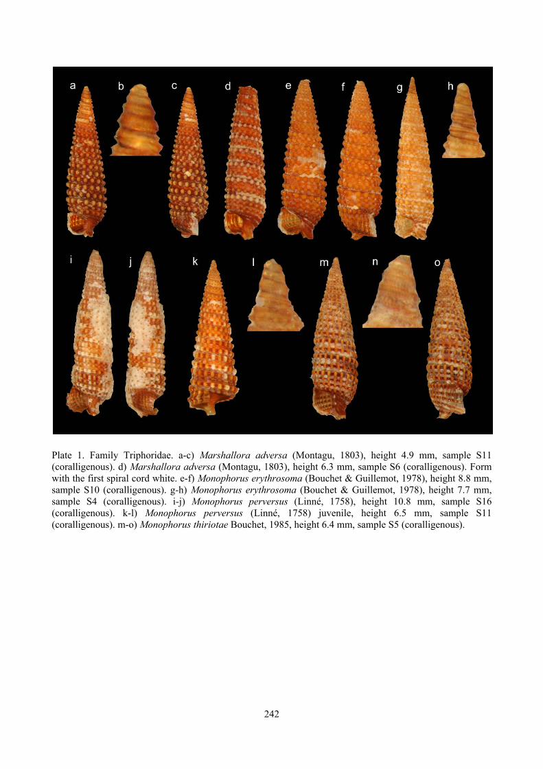
242

Plate 1. Family Triphoridae. a-c) Marshallora adversa (Montagu, 1803), height 4.9 mm, sample S11 (coralligenous). d) Marshallora adversa (Montagu, 1803), height 6.3 mm, sample S6 (coralligenous). Form with the first spiral cord white. e-f) Monophorus erythrosoma (Bouchet & Guillemot, 1978), height 8.8 mm, sample S10 (coralligenous). g-h) Monophorus erythrosoma (Bouchet & Guillemot, 1978), height 7.7 mm, sample S4 (coralligenous). i-j) Monophorus perversus (Linné, 1758), height 10.8 mm, sample S16 (coralligenous). k-l) Monophorus perversus (Linné, 1758) juvenile, height 6.5 mm, sample S11 (coralligenous). m-o) Monophorus thiriotae Bouchet, 1985, height 6.4 mm, sample S5 (coralligenous).

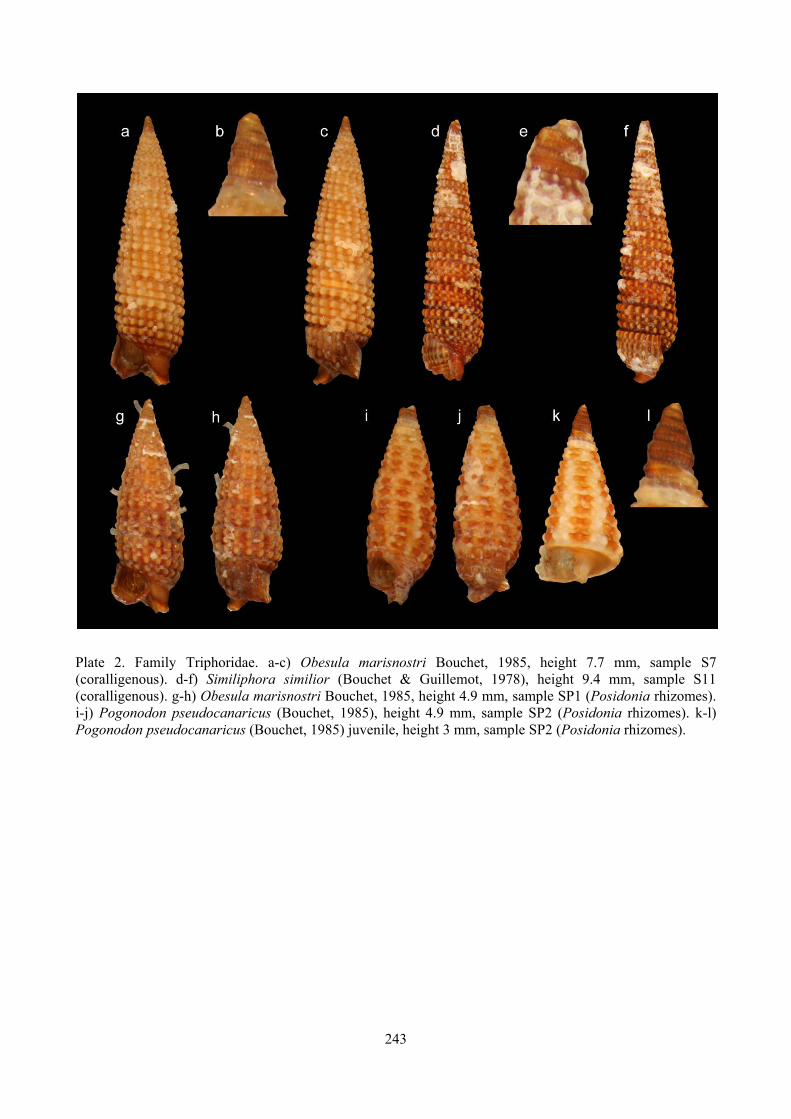
243

Plate 2. Family Triphoridae. a-c) Obesula marisnostri Bouchet, 1985, height 7.7 mm, sample S7 (coralligenous). d-f) Similiphora similior (Bouchet & Guillemot, 1978), height 9.4 mm, sample S11 (coralligenous). g-h) Obesula marisnostri Bouchet, 1985, height 4.9 mm, sample SP1 (Posidonia rhizomes). i-j) Pogonodon pseudocanaricus (Bouchet, 1985), height 4.9 mm, sample SP2 (Posidonia rhizomes). k-l) Pogonodon pseudocanaricus (Bouchet, 1985) juvenile, height 3 mm, sample SP2 (Posidonia rhizomes).

ANNEX 1

QUALI-QUANTITATIVE RESULTS OF THE MOLLUSCA SAMPLED

IN SECCHE DI TOR PATERNO

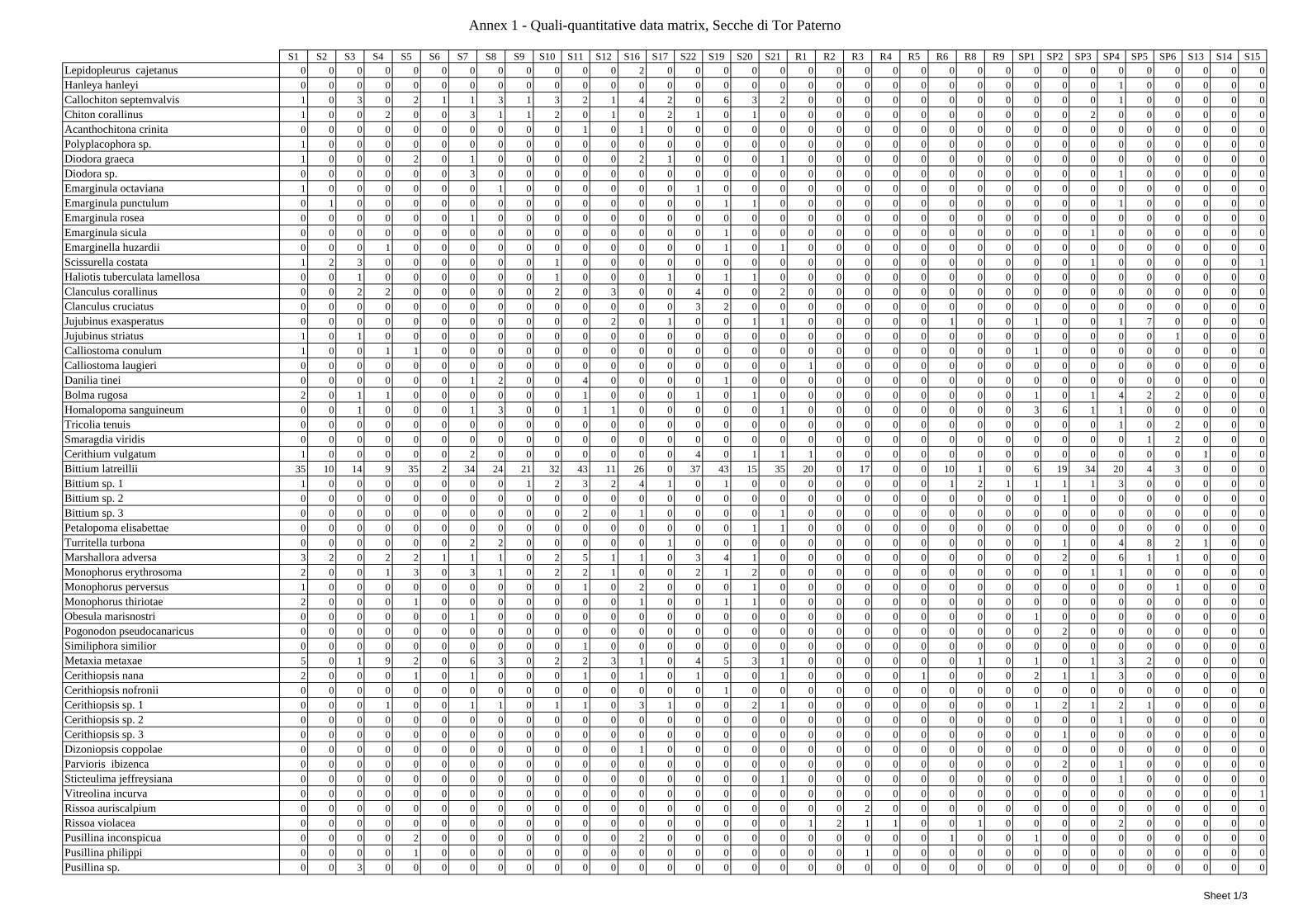
Annex 1 - Quali-quantitative data matrix, Secche di Tor Paterno

S1 S2 S3 S4 S5 S6 S7 S8 S9 S10 S11 S12 S16 S17 S22 S19 S20 S21 R1 R2 R3 R4 R5 R6 R8 R9 SP1 SP2 SP3 SP4 SP5 SP6 S13 S14 S15Lepidopleurus cajetanus 0 0 0 0 0 0 0 0 0 0 0 0 2 0 0 0 0 0 0 0 0 0 0 0 0 0 0 0 0 0 0 0 0 0 0Hanleya hanleyi 0 0 0 0 0 0 0 0 0 0 0 0 0 0 0 0 0 0 0 0 0 0 0 0 0 0 0 0 0 1 0 0 0 0 0Callochiton septemvalvis 1 0 3 0 2 1 1 3 1 3 2 1 4 2 0 6 3 2 0 0 0 0 0 0 0 0 0 0 0 1 0 0 0 0 0Chiton corallinus 1 0 0 2 0 0 3 1 1 2 0 1 0 2 1 0 1 0 0 0 0 0 0 0 0 0 0 0 2 0 0 0 0 0 0Acanthochitona crinita 0 0 0 0 0 0 0 0 0 0 1 0 1 0 0 0 0 0 0 0 0 0 0 0 0 0 0 0 0 0 0 0 0 0 0Polyplacophora sp. 1 0 0 0 0 0 0 0 0 0 0 0 0 0 0 0 0 0 0 0 0 0 0 0 0 0 0 0 0 0 0 0 0 0 0Diodora graeca 1 0 0 0 2 0 1 0 0 0 0 0 2 1 0 0 0 1 0 0 0 0 0 0 0 0 0 0 0 0 0 0 0 0 0Diodora sp. 0 0 0 0 0 0 3 0 0 0 0 0 0 0 0 0 0 0 0 0 0 0 0 0 0 0 0 0 0 1 0 0 0 0 0Emarginula octaviana 1 0 0 0 0 0 0 1 0 0 0 0 0 0 1 0 0 0 0 0 0 0 0 0 0 0 0 0 0 0 0 0 0 0 0Emarginula punctulum 0 1 0 0 0 0 0 0 0 0 0 0 0 0 0 1 1 0 0 0 0 0 0 0 0 0 0 0 0 1 0 0 0 0 0Emarginula rosea 0 0 0 0 0 0 1 0 0 0 0 0 0 0 0 0 0 0 0 0 0 0 0 0 0 0 0 0 0 0 0 0 0 0 0Emarginula sicula 0 0 0 0 0 0 0 0 0 0 0 0 0 0 0 1 0 0 0 0 0 0 0 0 0 0 0 0 1 0 0 0 0 0 0Emarginella huzardii 0 0 0 1 0 0 0 0 0 0 0 0 0 0 0 1 0 1 0 0 0 0 0 0 0 0 0 0 0 0 0 0 0 0 0Scissurella costata 1 2 3 0 0 0 0 0 0 1 0 0 0 0 0 0 0 0 0 0 0 0 0 0 0 0 0 0 1 0 0 0 0 0 1Haliotis tuberculata lamellosa 0 0 1 0 0 0 0 0 0 1 0 0 0 1 0 1 1 0 0 0 0 0 0 0 0 0 0 0 0 0 0 0 0 0 0Clanculus corallinus 0 0 2 2 0 0 0 0 0 2 0 3 0 0 4 0 0 2 0 0 0 0 0 0 0 0 0 0 0 0 0 0 0 0 0Clanculus cruciatus 0 0 0 0 0 0 0 0 0 0 0 0 0 0 3 2 0 0 0 0 0 0 0 0 0 0 0 0 0 0 0 0 0 0 0Jujubinus exasperatus 0 0 0 0 0 0 0 0 0 0 0 2 0 1 0 0 1 1 0 0 0 0 0 1 0 0 1 0 0 1 7 0 0 0 0Jujubinus striatus 1 0 1 0 0 0 0 0 0 0 0 0 0 0 0 0 0 0 0 0 0 0 0 0 0 0 0 0 0 0 0 1 0 0 0Calliostoma conulum 1 0 0 1 1 0 0 0 0 0 0 0 0 0 0 0 0 0 0 0 0 0 0 0 0 0 1 0 0 0 0 0 0 0 0Calliostoma laugieri 0 0 0 0 0 0 0 0 0 0 0 0 0 0 0 0 0 0 1 0 0 0 0 0 0 0 0 0 0 0 0 0 0 0 0Danilia tinei 0 0 0 0 0 0 1 2 0 0 4 0 0 0 0 1 0 0 0 0 0 0 0 0 0 0 0 0 0 0 0 0 0 0 0Bolma rugosa 2 0 1 1 0 0 0 0 0 0 1 0 0 0 1 0 1 0 0 0 0 0 0 0 0 0 1 0 1 4 2 2 0 0 0Homalopoma sanguineum 0 0 1 0 0 0 1 3 0 0 1 1 0 0 0 0 0 1 0 0 0 0 0 0 0 0 3 6 1 1 0 0 0 0 0Tricolia tenuis 0 0 0 0 0 0 0 0 0 0 0 0 0 0 0 0 0 0 0 0 0 0 0 0 0 0 0 0 0 1 0 2 0 0 0Smaragdia viridis 0 0 0 0 0 0 0 0 0 0 0 0 0 0 0 0 0 0 0 0 0 0 0 0 0 0 0 0 0 0 1 2 0 0 0Cerithium vulgatum 1 0 0 0 0 0 2 0 0 0 0 0 0 0 4 0 1 1 1 0 0 0 0 0 0 0 0 0 0 0 0 0 1 0 0Bittium latreillii 35 10 14 9 35 2 34 24 21 32 43 11 26 0 37 43 15 35 20 0 17 0 0 10 1 0 6 19 34 20 4 3 0 0 0Bittium sp. 1 1 0 0 0 0 0 0 0 1 2 3 2 4 1 0 1 0 0 0 0 0 0 0 1 2 1 1 1 1 3 0 0 0 0 0Bittium sp. 2 0 0 0 0 0 0 0 0 0 0 0 0 0 0 0 0 0 0 0 0 0 0 0 0 0 0 0 1 0 0 0 0 0 0 0Bittium sp. 3 0 0 0 0 0 0 0 0 0 0 2 0 1 0 0 0 0 1 0 0 0 0 0 0 0 0 0 0 0 0 0 0 0 0 0Petalopoma elisabettae 0 0 0 0 0 0 0 0 0 0 0 0 0 0 0 0 1 1 0 0 0 0 0 0 0 0 0 0 0 0 0 0 0 0 0Turritella turbona 0 0 0 0 0 0 2 2 0 0 0 0 0 1 0 0 0 0 0 0 0 0 0 0 0 0 0 1 0 4 8 2 1 0 0Marshallora adversa 3 2 0 2 2 1 1 1 0 2 5 1 1 0 3 4 1 0 0 0 0 0 0 0 0 0 0 2 0 6 1 1 0 0 0Monophorus erythrosoma 2 0 0 1 3 0 3 1 0 2 2 1 0 0 2 1 2 0 0 0 0 0 0 0 0 0 0 0 1 1 0 0 0 0 0Monophorus perversus 1 0 0 0 0 0 0 0 0 0 1 0 2 0 0 0 1 0 0 0 0 0 0 0 0 0 0 0 0 0 0 1 0 0 0Monophorus thiriotae 2 0 0 0 1 0 0 0 0 0 0 0 1 0 0 1 1 0 0 0 0 0 0 0 0 0 0 0 0 0 0 0 0 0 0Obesula marisnostri 0 0 0 0 0 0 1 0 0 0 0 0 0 0 0 0 0 0 0 0 0 0 0 0 0 0 1 0 0 0 0 0 0 0 0Pogonodon pseudocanaricus 0 0 0 0 0 0 0 0 0 0 0 0 0 0 0 0 0 0 0 0 0 0 0 0 0 0 0 2 0 0 0 0 0 0 0Similiphora similior 0 0 0 0 0 0 0 0 0 0 1 0 0 0 0 0 0 0 0 0 0 0 0 0 0 0 0 0 0 0 0 0 0 0 0Metaxia metaxae 5 0 1 9 2 0 6 3 0 2 2 3 1 0 4 5 3 1 0 0 0 0 0 0 1 0 1 0 1 3 2 0 0 0 0Cerithiopsis nana 2 0 0 0 1 0 1 0 0 0 1 0 1 0 1 0 0 1 0 0 0 0 1 0 0 0 2 1 1 3 0 0 0 0 0Cerithiopsis nofronii 0 0 0 0 0 0 0 0 0 0 0 0 0 0 0 1 0 0 0 0 0 0 0 0 0 0 0 0 0 0 0 0 0 0 0Cerithiopsis sp. 1 0 0 0 1 0 0 1 1 0 1 1 0 3 1 0 0 2 1 0 0 0 0 0 0 0 0 1 2 1 2 1 0 0 0 0Cerithiopsis sp. 2 0 0 0 0 0 0 0 0 0 0 0 0 0 0 0 0 0 0 0 0 0 0 0 0 0 0 0 0 0 1 0 0 0 0 0Cerithiopsis sp. 3 0 0 0 0 0 0 0 0 0 0 0 0 0 0 0 0 0 0 0 0 0 0 0 0 0 0 0 1 0 0 0 0 0 0 0Dizoniopsis coppolae 0 0 0 0 0 0 0 0 0 0 0 0 1 0 0 0 0 0 0 0 0 0 0 0 0 0 0 0 0 0 0 0 0 0 0Parvioris ibizenca 0 0 0 0 0 0 0 0 0 0 0 0 0 0 0 0 0 0 0 0 0 0 0 0 0 0 0 2 0 1 0 0 0 0 0Sticteulima jeffreysiana 0 0 0 0 0 0 0 0 0 0 0 0 0 0 0 0 0 1 0 0 0 0 0 0 0 0 0 0 0 1 0 0 0 0 0Vitreolina incurva 0 0 0 0 0 0 0 0 0 0 0 0 0 0 0 0 0 0 0 0 0 0 0 0 0 0 0 0 0 0 0 0 0 0 1Rissoa auriscalpium 0 0 0 0 0 0 0 0 0 0 0 0 0 0 0 0 0 0 0 0 2 0 0 0 0 0 0 0 0 0 0 0 0 0 0Rissoa violacea 0 0 0 0 0 0 0 0 0 0 0 0 0 0 0 0 0 0 1 2 1 1 0 0 1 0 0 0 0 2 0 0 0 0 0Pusillina inconspicua 0 0 0 0 2 0 0 0 0 0 0 0 2 0 0 0 0 0 0 0 0 0 0 1 0 0 1 0 0 0 0 0 0 0 0Pusillina philippi 0 0 0 0 1 0 0 0 0 0 0 0 0 0 0 0 0 0 0 0 1 0 0 0 0 0 0 0 0 0 0 0 0 0 0Pusillina sp. 0 0 3 0 0 0 0 0 0 0 0 0 0 0 0 0 0 0 0 0 0 0 0 0 0 0 0 0 0 0 0 0 0 0 0

Sheet 1/3

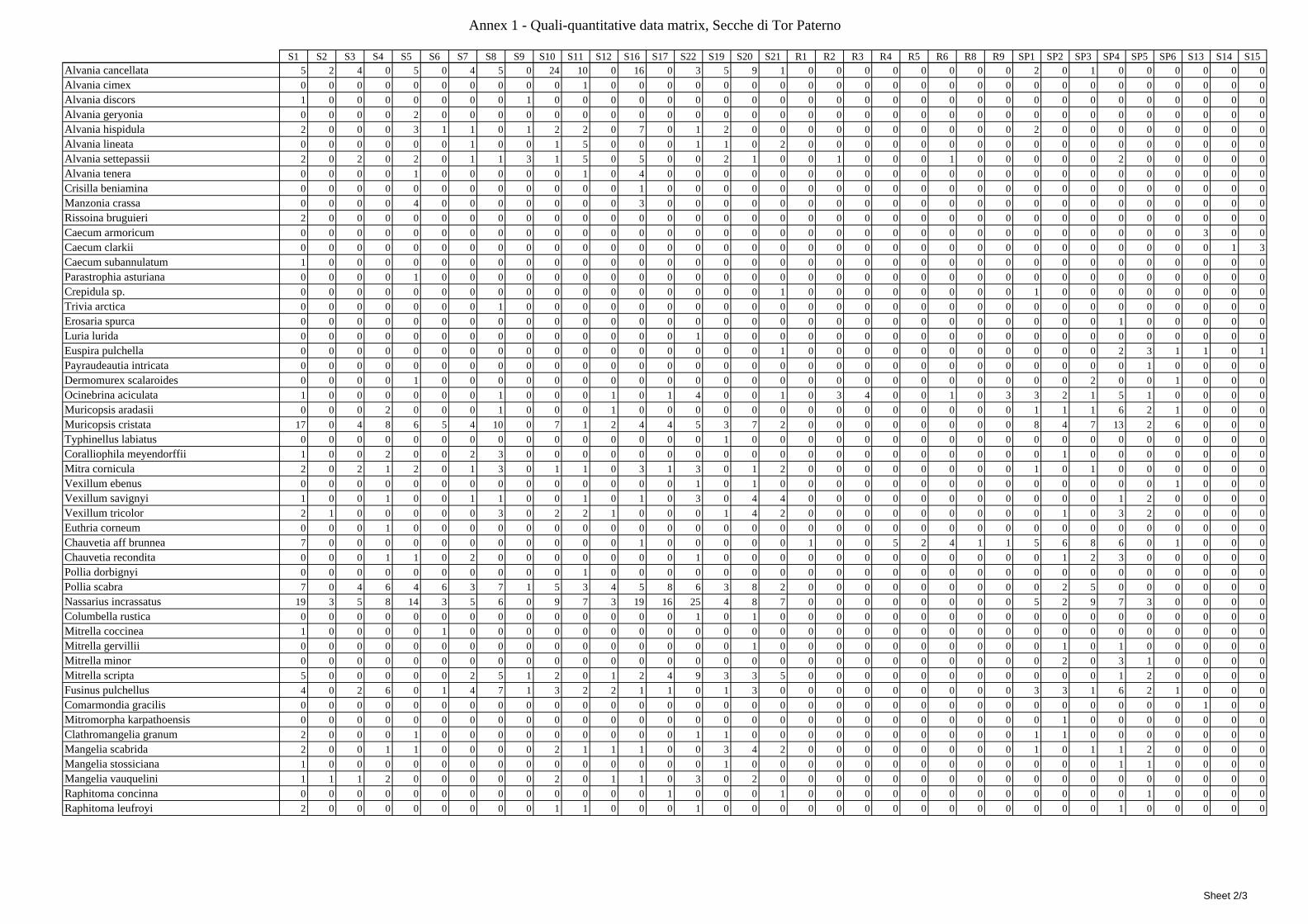
Annex 1 - Quali-quantitative data matrix, Secche di Tor Paterno

S1 S2 S3 S4 S5 S6 S7 S8 S9 S10 S11 S12 S16 S17 S22 S19 S20 S21 R1 R2 R3 R4 R5 R6 R8 R9 SP1 SP2 SP3 SP4 SP5 SP6 S13 S14 S15Alvania cancellata 5 2 4 0 5 0 4 5 0 24 10 0 16 0 3 5 9 1 0 0 0 0 0 0 0 0 2 0 1 0 0 0 0 0 0Alvania cimex 0 0 0 0 0 0 0 0 0 0 1 0 0 0 0 0 0 0 0 0 0 0 0 0 0 0 0 0 0 0 0 0 0 0 0Alvania discors 1 0 0 0 0 0 0 0 1 0 0 0 0 0 0 0 0 0 0 0 0 0 0 0 0 0 0 0 0 0 0 0 0 0 0Alvania geryonia 0 0 0 0 2 0 0 0 0 0 0 0 0 0 0 0 0 0 0 0 0 0 0 0 0 0 0 0 0 0 0 0 0 0 0Alvania hispidula 2 0 0 0 3 1 1 0 1 2 2 0 7 0 1 2 0 0 0 0 0 0 0 0 0 0 2 0 0 0 0 0 0 0 0Alvania lineata 0 0 0 0 0 0 1 0 0 1 5 0 0 0 1 1 0 2 0 0 0 0 0 0 0 0 0 0 0 0 0 0 0 0 0Alvania settepassii 2 0 2 0 2 0 1 1 3 1 5 0 5 0 0 2 1 0 0 1 0 0 0 1 0 0 0 0 0 2 0 0 0 0 0Alvania tenera 0 0 0 0 1 0 0 0 0 0 1 0 4 0 0 0 0 0 0 0 0 0 0 0 0 0 0 0 0 0 0 0 0 0 0Crisilla beniamina 0 0 0 0 0 0 0 0 0 0 0 0 1 0 0 0 0 0 0 0 0 0 0 0 0 0 0 0 0 0 0 0 0 0 0Manzonia crassa 0 0 0 0 4 0 0 0 0 0 0 0 3 0 0 0 0 0 0 0 0 0 0 0 0 0 0 0 0 0 0 0 0 0 0Rissoina bruguieri 2 0 0 0 0 0 0 0 0 0 0 0 0 0 0 0 0 0 0 0 0 0 0 0 0 0 0 0 0 0 0 0 0 0 0Caecum armoricum 0 0 0 0 0 0 0 0 0 0 0 0 0 0 0 0 0 0 0 0 0 0 0 0 0 0 0 0 0 0 0 0 3 0 0Caecum clarkii 0 0 0 0 0 0 0 0 0 0 0 0 0 0 0 0 0 0 0 0 0 0 0 0 0 0 0 0 0 0 0 0 0 1 3Caecum subannulatum 1 0 0 0 0 0 0 0 0 0 0 0 0 0 0 0 0 0 0 0 0 0 0 0 0 0 0 0 0 0 0 0 0 0 0Parastrophia asturiana 0 0 0 0 1 0 0 0 0 0 0 0 0 0 0 0 0 0 0 0 0 0 0 0 0 0 0 0 0 0 0 0 0 0 0Crepidula sp. 0 0 0 0 0 0 0 0 0 0 0 0 0 0 0 0 0 1 0 0 0 0 0 0 0 0 1 0 0 0 0 0 0 0 0Trivia arctica 0 0 0 0 0 0 0 1 0 0 0 0 0 0 0 0 0 0 0 0 0 0 0 0 0 0 0 0 0 0 0 0 0 0 0Erosaria spurca 0 0 0 0 0 0 0 0 0 0 0 0 0 0 0 0 0 0 0 0 0 0 0 0 0 0 0 0 0 1 0 0 0 0 0Luria lurida 0 0 0 0 0 0 0 0 0 0 0 0 0 0 1 0 0 0 0 0 0 0 0 0 0 0 0 0 0 0 0 0 0 0 0Euspira pulchella 0 0 0 0 0 0 0 0 0 0 0 0 0 0 0 0 0 1 0 0 0 0 0 0 0 0 0 0 0 2 3 1 1 0 1Payraudeautia intricata 0 0 0 0 0 0 0 0 0 0 0 0 0 0 0 0 0 0 0 0 0 0 0 0 0 0 0 0 0 0 1 0 0 0 0Dermomurex scalaroides 0 0 0 0 1 0 0 0 0 0 0 0 0 0 0 0 0 0 0 0 0 0 0 0 0 0 0 0 2 0 0 1 0 0 0Ocinebrina aciculata 1 0 0 0 0 0 0 1 0 0 0 1 0 1 4 0 0 1 0 3 4 0 0 1 0 3 3 2 1 5 1 0 0 0 0Muricopsis aradasii 0 0 0 2 0 0 0 1 0 0 0 1 0 0 0 0 0 0 0 0 0 0 0 0 0 0 1 1 1 6 2 1 0 0 0Muricopsis cristata 17 0 4 8 6 5 4 10 0 7 1 2 4 4 5 3 7 2 0 0 0 0 0 0 0 0 8 4 7 13 2 6 0 0 0Typhinellus labiatus 0 0 0 0 0 0 0 0 0 0 0 0 0 0 0 1 0 0 0 0 0 0 0 0 0 0 0 0 0 0 0 0 0 0 0Coralliophila meyendorffii 1 0 0 2 0 0 2 3 0 0 0 0 0 0 0 0 0 0 0 0 0 0 0 0 0 0 0 1 0 0 0 0 0 0 0Mitra cornicula 2 0 2 1 2 0 1 3 0 1 1 0 3 1 3 0 1 2 0 0 0 0 0 0 0 0 1 0 1 0 0 0 0 0 0Vexillum ebenus 0 0 0 0 0 0 0 0 0 0 0 0 0 0 1 0 1 0 0 0 0 0 0 0 0 0 0 0 0 0 0 1 0 0 0Vexillum savignyi 1 0 0 1 0 0 1 1 0 0 1 0 1 0 3 0 4 4 0 0 0 0 0 0 0 0 0 0 0 1 2 0 0 0 0Vexillum tricolor 2 1 0 0 0 0 0 3 0 2 2 1 0 0 0 1 4 2 0 0 0 0 0 0 0 0 0 1 0 3 2 0 0 0 0Euthria corneum 0 0 0 1 0 0 0 0 0 0 0 0 0 0 0 0 0 0 0 0 0 0 0 0 0 0 0 0 0 0 0 0 0 0 0Chauvetia aff brunnea 7 0 0 0 0 0 0 0 0 0 0 0 1 0 0 0 0 0 1 0 0 5 2 4 1 1 5 6 8 6 0 1 0 0 0Chauvetia recondita 0 0 0 1 1 0 2 0 0 0 0 0 0 0 1 0 0 0 0 0 0 0 0 0 0 0 0 1 2 3 0 0 0 0 0Pollia dorbignyi 0 0 0 0 0 0 0 0 0 0 1 0 0 0 0 0 0 0 0 0 0 0 0 0 0 0 0 0 0 0 0 0 0 0 0Pollia scabra 7 0 4 6 4 6 3 7 1 5 3 4 5 8 6 3 8 2 0 0 0 0 0 0 0 0 0 2 5 0 0 0 0 0 0Nassarius incrassatus 19 3 5 8 14 3 5 6 0 9 7 3 19 16 25 4 8 7 0 0 0 0 0 0 0 0 5 2 9 7 3 0 0 0 0Columbella rustica 0 0 0 0 0 0 0 0 0 0 0 0 0 0 1 0 1 0 0 0 0 0 0 0 0 0 0 0 0 0 0 0 0 0 0Mitrella coccinea 1 0 0 0 0 1 0 0 0 0 0 0 0 0 0 0 0 0 0 0 0 0 0 0 0 0 0 0 0 0 0 0 0 0 0Mitrella gervillii 0 0 0 0 0 0 0 0 0 0 0 0 0 0 0 0 1 0 0 0 0 0 0 0 0 0 0 1 0 1 0 0 0 0 0Mitrella minor 0 0 0 0 0 0 0 0 0 0 0 0 0 0 0 0 0 0 0 0 0 0 0 0 0 0 0 2 0 3 1 0 0 0 0Mitrella scripta 5 0 0 0 0 0 2 5 1 2 0 1 2 4 9 3 3 5 0 0 0 0 0 0 0 0 0 0 0 1 2 0 0 0 0Fusinus pulchellus 4 0 2 6 0 1 4 7 1 3 2 2 1 1 0 1 3 0 0 0 0 0 0 0 0 0 3 3 1 6 2 1 0 0 0Comarmondia gracilis 0 0 0 0 0 0 0 0 0 0 0 0 0 0 0 0 0 0 0 0 0 0 0 0 0 0 0 0 0 0 0 0 1 0 0Mitromorpha karpathoensis 0 0 0 0 0 0 0 0 0 0 0 0 0 0 0 0 0 0 0 0 0 0 0 0 0 0 0 1 0 0 0 0 0 0 0Clathromangelia granum 2 0 0 0 1 0 0 0 0 0 0 0 0 0 1 1 0 0 0 0 0 0 0 0 0 0 1 1 0 0 0 0 0 0 0Mangelia scabrida 2 0 0 1 1 0 0 0 0 2 1 1 1 0 0 3 4 2 0 0 0 0 0 0 0 0 1 0 1 1 2 0 0 0 0Mangelia stossiciana 1 0 0 0 0 0 0 0 0 0 0 0 0 0 0 1 0 0 0 0 0 0 0 0 0 0 0 0 0 1 1 0 0 0 0Mangelia vauquelini 1 1 1 2 0 0 0 0 0 2 0 1 1 0 3 0 2 0 0 0 0 0 0 0 0 0 0 0 0 0 0 0 0 0 0Raphitoma concinna 0 0 0 0 0 0 0 0 0 0 0 0 0 1 0 0 0 1 0 0 0 0 0 0 0 0 0 0 0 0 1 0 0 0 0Raphitoma leufroyi 2 0 0 0 0 0 0 0 0 1 1 0 0 0 1 0 0 0 0 0 0 0 0 0 0 0 0 0 0 1 0 0 0 0 0

Sheet 2/3

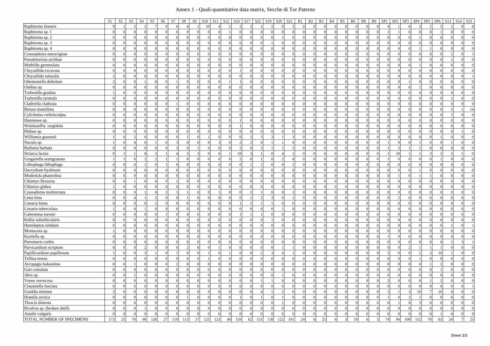
Annex 1 - Quali-quantitative data matrix, Secche di Tor Paterno

S1 S2 S3 S4 S5 S6 S7 S8 S9 S10 S11 S12 S16 S17 S22 S19 S20 S21 R1 R2 R3 R4 R5 R6 R8 R9 SP1 SP2 SP3 SP4 SP5 SP6 S13 S14 S15Raphitoma linearis 9 1 2 2 7 0 6 4 1 10 4 2 2 2 1 2 9 5 0 0 0 0 0 0 0 0 4 1 6 3 1 5 1 0 0Raphitoma sp. 1 0 0 0 0 0 0 0 0 0 0 0 1 0 0 0 0 0 0 0 0 0 0 0 0 0 0 2 1 0 0 0 1 0 0 0Raphitoma sp. 2 0 0 0 0 0 0 0 0 0 0 0 0 0 0 0 0 1 0 0 0 0 0 0 0 0 0 0 0 0 1 0 0 0 0 0Raphitoma sp. 3 0 0 0 0 0 0 0 0 0 0 0 0 0 0 0 1 0 0 0 0 0 0 0 0 0 0 0 0 0 0 0 0 0 0 0Raphitoma sp. 4 0 0 0 0 0 0 0 0 0 0 0 0 0 0 0 0 0 0 0 0 0 0 0 0 0 0 0 0 0 1 1 0 0 0 0Crassopleura maravignae 0 0 0 0 0 0 0 0 0 0 0 0 0 0 0 0 0 0 0 0 0 0 0 0 0 0 0 0 0 0 0 0 2 0 1Pseudotorinia architae 0 0 0 0 0 0 0 0 0 0 0 0 0 0 0 0 0 0 0 0 0 0 0 0 0 0 0 0 0 0 0 0 1 0 0Mathilda gemmulata 0 0 0 0 0 0 0 0 0 0 0 0 0 0 0 0 0 0 0 0 0 0 0 0 0 0 0 0 0 1 0 0 0 0 0Chrysallida excavata 0 0 0 0 0 0 0 0 0 0 0 0 1 0 0 0 0 0 0 0 0 0 0 0 0 0 0 0 0 0 0 0 0 0 0Chrysallida suturalis 2 0 0 0 0 0 0 0 0 0 0 0 0 0 0 0 0 0 0 0 0 0 0 0 0 0 0 0 0 0 0 0 0 0 1Odostomella doliolum 2 0 0 1 8 0 1 0 0 0 0 1 1 0 0 0 0 0 0 0 0 0 0 0 0 0 0 0 1 0 0 0 0 0 0Ondina sp. 0 0 0 0 0 0 0 0 0 0 0 0 0 0 0 0 0 0 0 0 0 0 0 0 0 0 0 0 0 1 0 0 0 0 0Turbonilla gradata 1 0 0 0 0 0 0 0 0 0 0 0 0 0 0 0 0 0 0 0 0 0 0 0 0 0 0 0 0 0 0 0 0 0 0Turbonilla striatula 0 0 0 0 0 0 0 0 0 0 0 0 0 0 0 0 0 0 0 0 0 0 0 0 0 0 0 0 0 0 0 0 1 0 0Clathrella clathrata 0 0 0 0 0 0 1 0 0 0 0 0 0 0 0 0 0 0 0 0 0 0 0 0 0 0 0 0 0 0 0 0 0 0 0Retusa mamillata 0 0 0 0 0 0 0 0 0 0 0 0 0 0 0 0 0 0 0 0 0 0 0 0 0 0 0 0 0 0 0 0 5 1 14Cylichnina crebrisculpta 0 0 0 0 0 0 0 0 0 0 0 0 0 0 0 0 0 0 0 0 0 0 0 0 0 0 0 0 0 0 0 0 1 0 0Haminoea sp. 0 0 0 0 0 0 0 0 0 0 0 0 1 0 0 0 0 0 0 0 0 0 0 0 0 0 0 0 0 0 0 0 0 0 0Weinkauffia turgidula 0 0 0 0 0 0 0 0 0 0 0 0 1 0 0 0 0 0 0 0 0 0 0 0 0 0 0 0 0 0 0 0 0 0 0Philine sp. 0 0 0 0 0 0 0 0 0 0 0 0 0 0 0 0 0 0 0 0 0 0 0 0 0 0 0 0 0 0 0 0 0 1 0Williamia gussonii 1 0 2 0 0 0 0 1 0 1 0 0 0 2 3 3 1 3 0 0 0 0 0 0 0 0 0 0 0 0 0 1 0 0 0Nucula sp. 1 0 4 0 1 0 3 0 0 0 3 0 2 2 0 1 1 0 0 0 0 0 0 0 0 0 1 0 0 1 0 0 1 0 0Barbatia barbata 0 0 0 0 0 0 3 0 1 0 0 0 2 0 3 1 1 2 0 0 0 0 0 0 0 0 1 3 1 2 0 0 0 0 0Striarca lactea 0 1 1 8 3 1 4 3 3 0 0 1 18 3 1 0 4 1 0 0 0 0 0 0 0 0 1 18 1 1 3 2 2 1 0Gregariella semigranata 1 1 0 1 2 1 1 0 0 0 0 0 2 0 1 0 2 0 0 0 0 0 0 0 0 0 1 0 0 0 0 1 0 0 0Lithophaga lithophaga 0 0 0 1 0 1 0 0 0 0 0 0 0 1 1 0 0 2 0 0 0 0 0 0 0 0 0 0 0 0 0 0 0 0 0Dacrydium hyalinum 0 0 0 0 0 0 0 0 0 0 0 0 0 0 0 0 0 0 0 0 0 0 0 0 0 0 0 0 0 1 0 0 0 0 0Modiolula phaseolina 0 0 0 0 0 0 0 0 0 0 0 0 0 0 0 0 0 0 0 0 0 0 0 0 0 0 0 1 0 1 1 0 0 0 0Chlamys flexuosa 0 0 1 0 0 0 1 0 0 0 0 0 0 0 0 0 0 0 0 0 0 0 0 0 0 0 0 0 0 0 0 0 0 0 0Chlamys glabra 1 0 0 0 0 0 0 0 0 0 0 0 0 0 0 0 0 0 0 0 0 0 0 0 0 0 0 0 0 0 0 0 0 0 0Crassadoma multistriata 0 0 0 1 0 2 3 1 0 0 1 0 0 2 1 0 0 2 0 0 0 0 0 0 0 0 0 0 0 0 0 0 0 0 0Lima lima 0 0 4 1 2 0 0 1 0 0 0 0 0 1 2 3 0 1 0 0 0 0 0 0 0 0 0 2 0 0 0 0 0 0 0Limaria hians 0 0 0 0 2 0 0 0 0 0 0 0 1 2 1 1 0 0 0 0 0 0 0 0 0 0 0 0 0 0 0 0 0 0 0Limaria tuberculata 1 0 0 1 0 0 0 0 0 0 0 0 0 0 0 0 1 0 0 0 0 0 0 0 0 0 0 0 0 0 0 0 0 0 0Galeomma turtoni 0 0 0 0 0 1 0 4 0 0 0 0 1 1 1 0 0 0 0 0 0 0 0 0 0 0 0 0 0 0 0 0 0 0 0Kellia suborbicularis 0 0 0 0 0 0 0 0 0 0 0 0 0 0 0 1 0 0 0 0 0 0 0 0 0 0 0 0 0 0 0 0 0 0 0Hemilepton nitidum 0 0 0 0 0 0 0 0 0 0 0 0 0 0 0 0 0 0 0 0 0 0 0 0 0 0 0 0 0 0 0 0 1 0 1Montacuta sp. 1 0 0 0 0 0 0 0 0 0 0 0 0 0 0 0 0 0 0 0 0 0 0 0 0 0 0 0 0 0 0 0 0 0 0Kurtiella sp. 0 0 0 0 0 0 0 0 0 0 0 0 0 0 0 0 0 0 0 0 0 0 0 0 0 0 1 0 0 0 0 0 0 0 0Pteromeris corbis 0 0 0 0 0 0 0 0 0 0 0 0 0 0 0 0 0 0 0 0 0 0 0 0 0 0 0 0 0 0 0 0 1 3 1Parvicardium scriptum 0 0 0 2 0 0 0 2 0 0 1 0 0 0 0 0 1 1 0 0 0 0 0 0 0 0 0 0 2 1 1 1 0 0 0Papillicardium papillosum 1 0 0 3 1 0 1 0 0 1 0 1 0 0 2 3 4 1 0 0 0 0 0 0 0 0 5 0 0 2 3 10 1 0 0Tellina tenuis 0 0 0 0 0 0 0 0 0 1 0 0 0 0 0 0 0 0 0 0 0 0 0 0 0 0 0 0 0 1 0 0 0 0 0Arcopagia balaustina 0 0 1 0 0 0 2 0 0 0 0 0 0 0 0 0 0 0 0 0 0 0 0 0 0 0 0 0 0 0 1 2 0 0 0Gari costulata 0 0 0 0 0 0 0 0 0 0 0 0 0 0 0 0 0 0 0 0 0 0 0 0 0 0 0 0 0 0 0 1 0 0 0Abra sp. 0 0 1 0 0 0 0 0 0 0 0 0 0 0 0 0 1 0 0 0 0 0 0 0 0 0 0 0 0 0 0 0 0 0 0Venus verrucosa 0 0 0 0 0 0 0 0 0 0 0 0 0 0 1 1 0 0 0 0 0 0 0 0 0 0 2 0 0 0 1 2 0 0 0Clausinella fasciata 0 0 0 0 0 0 0 0 0 0 0 0 0 0 0 0 0 0 0 0 0 0 0 0 0 0 0 0 0 0 0 0 0 0 1Gouldia minima 2 0 0 0 0 0 0 0 0 0 0 0 0 0 4 1 2 0 0 0 0 0 0 0 0 0 3 1 3 10 7 10 0 0 0Hiatella arctica 0 0 0 0 0 0 0 1 0 0 0 0 1 0 1 0 1 0 0 0 0 0 0 0 0 0 1 0 2 1 0 0 0 0 0Thracia distorta 0 0 0 0 0 0 0 0 0 0 0 0 0 0 0 0 1 0 0 0 0 0 0 0 0 0 0 1 0 3 0 0 0 0 0Bivalvia sp. (broken shell) 0 0 0 1 0 0 0 0 0 0 0 0 0 0 0 0 0 0 0 0 0 0 0 0 0 0 0 0 0 0 0 0 0 0 0Antalis vulgaris 0 0 0 0 0 0 0 0 0 0 0 0 0 0 0 0 0 0 0 0 0 0 0 0 0 0 0 0 0 0 0 1 0 0 0TOTAL NUMBER OF SPECIMENS 173 25 70 90 126 27 119 113 37 125 123 49 159 62 153 118 122 101 24 6 25 6 3 19 6 5 74 94 100 152 70 63 24 7 25

Sheet 3/3

ANNEX 2

QUALI-QUANTITATIVE RESULTS OF THE SAMPLING IN POSIDONIA OCEANICA

IN SECCHE DELLA MELORIA (BOTH LEAVES AND RHIZOMES,

CASTRIOTA, 1989)

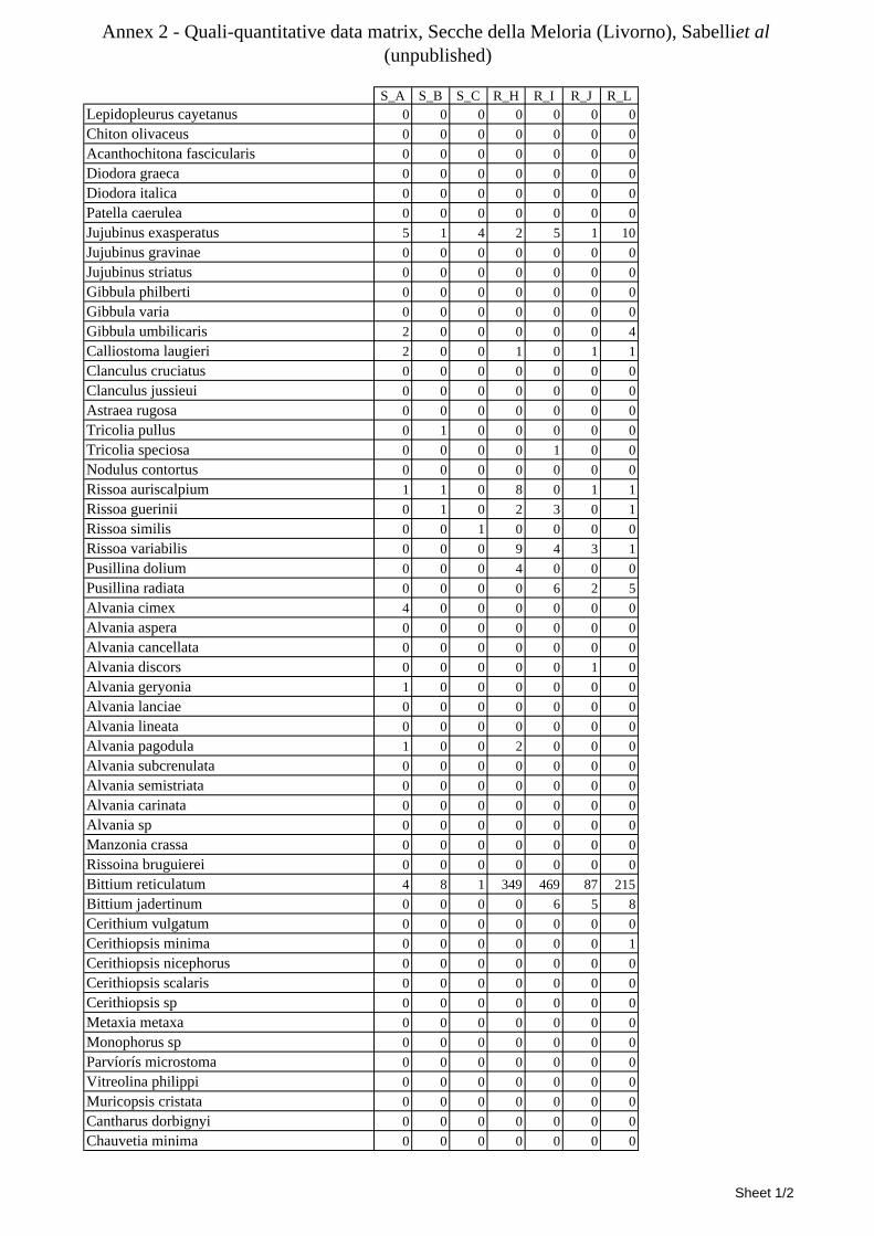
Annex 2 - Quali-quantitative data matrix, Secche della Meloria (Livorno), Sabelli et al (unpublished)

S_A S_B S_C R_H R_I R_J R_LLepidopleurus cayetanus 0 0 0 0 0 0 0Chiton olivaceus 0 0 0 0 0 0 0Acanthochitona fascicularis 0 0 0 0 0 0 0Diodora graeca 0 0 0 0 0 0 0Diodora italica 0 0 0 0 0 0 0Patella caerulea 0 0 0 0 0 0 0Jujubinus exasperatus 5 1 4 2 5 1 10Jujubinus gravinae 0 0 0 0 0 0 0Jujubinus striatus 0 0 0 0 0 0 0Gibbula philberti 0 0 0 0 0 0 0Gibbula varia 0 0 0 0 0 0 0Gibbula umbilicaris 2 0 0 0 0 0 4Calliostoma laugieri 2 0 0 1 0 1 1Clanculus cruciatus 0 0 0 0 0 0 0Clanculus jussieui 0 0 0 0 0 0 0Astraea rugosa 0 0 0 0 0 0 0Tricolia pullus 0 1 0 0 0 0 0Tricolia speciosa 0 0 0 0 1 0 0Nodulus contortus 0 0 0 0 0 0 0Rissoa auriscalpium 1 1 0 8 0 1 1Rissoa guerinii 0 1 0 2 3 0 1Rissoa similis 0 0 1 0 0 0 0Rissoa variabilis 0 0 0 9 4 3 1Pusillina dolium 0 0 0 4 0 0 0Pusillina radiata 0 0 0 0 6 2 5Alvania cimex 4 0 0 0 0 0 0Alvania aspera 0 0 0 0 0 0 0Alvania cancellata 0 0 0 0 0 0 0Alvania discors 0 0 0 0 0 1 0Alvania geryonia 1 0 0 0 0 0 0Alvania lanciae 0 0 0 0 0 0 0Alvania lineata 0 0 0 0 0 0 0Alvania pagodula 1 0 0 2 0 0 0Alvania subcrenulata 0 0 0 0 0 0 0Alvania semistriata 0 0 0 0 0 0 0Alvania carinata 0 0 0 0 0 0 0Alvania sp 0 0 0 0 0 0 0Manzonia crassa 0 0 0 0 0 0 0Rissoina bruguierei 0 0 0 0 0 0 0Bittium reticulatum 4 8 1 349 469 87 215Bittium jadertinum 0 0 0 0 6 5 8Cerithium vulgatum 0 0 0 0 0 0 0Cerithiopsis minima 0 0 0 0 0 0 1Cerithiopsis nicephorus 0 0 0 0 0 0 0Cerithiopsis scalaris 0 0 0 0 0 0 0Cerithiopsis sp 0 0 0 0 0 0 0Metaxia metaxa 0 0 0 0 0 0 0Monophorus sp 0 0 0 0 0 0 0Parvíorís microstoma 0 0 0 0 0 0 0Vitreolina philippi 0 0 0 0 0 0 0Muricopsis cristata 0 0 0 0 0 0 0Cantharus dorbignyi 0 0 0 0 0 0 0Chauvetia minima 0 0 0 0 0 0 0

Sheet 1/2

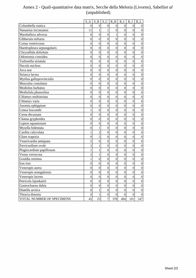
Annex 2 - Quali-quantitative data matrix, Secche della Meloria (Livorno), Sabelli et al (unpublished)

S_A S_B S_C R_H R_I R_J R_LColumbella rustica 0 0 0 0 0 0 0Nassarius incrassatus 11 1 1 0 0 0 0Marshallora adversa 0 0 0 1 0 0 0Gíbberula miliaria 0 0 0 0 0 0 0Conus ventricosus 0 0 0 0 0 0 0Haedropleura septangularis 0 0 0 0 0 0 0Chrysallida doliolum 0 0 0 0 0 0 0Odostomia conoidea 0 0 0 0 0 0 0Turbonilla striatula 0 0 0 0 0 0 0Nucula nucleus 0 0 0 0 0 0 0Arca noe 0 0 0 0 0 0 0Striarca lactea 0 0 0 0 0 0 0Mytilus galloprovincialis 0 0 0 0 0 0 0Musculus costulatus 0 0 0 0 0 0 0Modiolus barbatus 0 0 0 0 0 0 0Modiolula phaseolina 0 0 0 0 0 0 0Chlamys multistriata 0 0 0 0 0 0 0ChIamys varia 0 0 0 0 0 0 0Anomia ephippium 0 0 0 0 0 0 0Limea loscombi 1 0 0 0 0 0 0Ctena decussata 0 0 0 0 0 0 0Chama gryphoides 0 0 0 0 0 0 0Lepton squamosum 0 0 0 0 0 0 0Mysella bidentata 0 1 0 0 0 0 0Cardita calyculata 1 2 0 0 0 0 0Glans trapezia 0 2 0 0 0 0 0Venericardia antiquata 5 0 0 0 0 0 0Parvicardium ovale 3 1 0 0 0 0 0Plagiocardium papillosum 1 1 0 0 0 0 0Venus verrucosa 2 1 0 0 0 0 0Gouldia minima 1 0 0 0 0 0 0Irus irus 0 0 0 0 0 0 0Venerupis aurea 0 0 0 0 0 0 0Venerupis senegalensis 0 0 0 0 0 0 0Venerupis lucens 0 0 0 0 0 0 0Petricola lajonkairii 0 0 0 0 0 0 0Gastrochaena dubia 0 0 0 0 0 0 0Hiatella arctica 0 1 0 0 0 0 0Thracia distorta 0 1 0 0 0 0 0TOTAL NUMBER OF SPECIMENS 45 23 7 378 494 101 247

Sheet 2/2

ANNEX 3

QUALI-QUANTITATIVE RESULTS OF THE SAMPLING IN POSIDONIA OCEANICA

IN ELBA ISLAND (BOTH LEAVES AND RHIZOMES,

B. SABELLI UNPUBLISHED DATA)

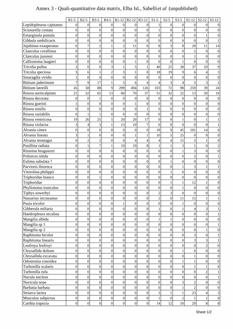
Annex 3 - Quali-quantitative data matrix, Elba Isl., Sabelli et al (unpublished)

R1-5 R2-5 R3-5 R4-5 R1-12 R2-12 R3-12 S1-5 S2-5 S3-5 S1-12 S2-12 S3-12Lepidopleurus cajetanus 0 0 0 0 0 0 0 1 0 0 0 0 0Scissurella costata 0 0 0 0 0 0 0 1 0 0 0 0 0Emarginula pustula 0 0 0 0 0 0 0 0 0 0 0 1 0Gibbula umbilicaris 0 0 0 0 0 0 0 0 0 0 0 0 1Jujubinus exasperatus 6 7 2 1 2 11 6 8 3 8 20 11 14Clanculus corallinus 0 0 0 0 0 0 0 0 0 0 2 0 0Clanculus jussieui 0 0 0 0 0 0 0 0 0 0 1 0 0Calliostoma laugieri 0 0 0 0 0 1 0 0 0 1 0 0 0Tricolia pullus 2 0 0 3 1 5 1 40 25 38 37 10 9Tricolia speciosa 5 6 1 2 3 1 0 18 19 9 6 4 3Smaragdia viridis 1 0 0 0 0 0 0 0 0 0 0 0 0Bittium jadertinum 7 9 17 1 5 6 4 4 3 4 5 3 2Bittium latreilli 45 58 88 9 299 494 126 103 72 98 259 39 24Rissoa auriscalpium 21 32 65 13 60 70 37 51 32 22 13 20 10Rissoa decorata 0 0 1 0 0 0 0 0 0 0 0 0 0Rissoa guerini 1 0 0 0 0 1 0 0 0 0 0 0 0Rissoa similis 0 0 0 0 0 0 1 0 0 0 0 0 0Rissoa variabilis 0 1 1 0 0 0 0 0 0 0 0 0 0Rissoa ventricosa 19 26 25 5 20 20 17 0 0 1 0 1 1Rissoa violacea 3 4 3 1 13 10 7 0 0 0 0 0 1Alvania cimex 0 0 0 0 0 0 0 18 9 45 101 14 0Alvania lineata 3 1 0 0 0 1 1 10 5 25 0 0 0Alvania montagui 0 2 2 0 0 4 4 4 4 15 2 1 0Pusillina radiata 0 1 7 1 19 19 8 1 1 3 1 0 2Rissoina bruguierei 0 0 0 0 0 0 0 0 0 1 3 0 0Polinices nitida 0 0 0 0 0 0 0 0 0 0 2 0 1Eulima subulata ? 0 0 0 0 0 0 0 0 1 0 0 0 0Parvioris ibizenca 0 0 0 0 0 0 0 0 0 1 3 1 1Vitreolina philippii 0 0 0 0 0 0 0 0 1 0 0 0 0Triphoridae bianco 0 0 1 0 0 0 0 0 0 0 0 0 0Triphoridae 0 0 0 0 0 0 0 0 1 1 12 1 0Phyllonotus trunculus 0 0 0 0 0 0 0 0 0 1 0 0 0Tiphys sowerbyi 0 0 0 0 0 0 0 2 3 0 0 0 0Nassarius incrassatus 0 0 0 0 0 0 0 2 0 11 15 1 1Pusia tricolor 0 0 0 0 1 0 0 0 0 1 0 0 0Gibberula miliaria 0 0 0 0 0 0 0 1 0 1 4 3 1Haedropleura secalina 0 0 0 0 0 0 0 0 0 0 0 0 1Mangilia albida 0 0 0 0 0 0 0 1 1 0 0 0 0Mangilia sp 1 0 0 0 0 0 0 0 0 0 0 0 0 1Mangilia sp 2 0 0 0 0 0 0 0 0 0 0 0 1 0Raphitoma bicolor 0 0 0 0 0 0 0 0 0 0 3 0 1Raphitoma linearis 0 0 0 0 0 0 0 0 0 0 3 3 1Leufroya leufroyi 0 0 0 0 0 0 0 0 0 0 0 2 0Chrysallida dolium 0 0 0 0 0 0 0 0 0 1 0 0 0Chrysallida excavata 0 0 0 0 0 0 0 0 0 0 1 0 0Odostomia conoidea 0 0 0 0 0 0 0 0 0 1 1 0 0Turbonilla scalaris 0 0 0 0 0 0 0 0 0 0 1 1 0Turbonilla rufa 0 0 0 0 0 0 0 0 0 0 0 2 1Nucula nucleus 0 0 0 0 0 0 0 0 0 0 0 0 1Navicula noae 0 0 0 0 0 0 0 0 0 3 2 0 0Barbatia barbata 0 0 0 0 0 0 0 0 0 1 2 0 0Striarca lactea 0 0 0 0 0 0 0 3 1 1 23 4 3Musculus subpictus 0 0 0 0 0 0 0 1 0 2 1 1 0Cardita trapezia 0 0 0 0 0 0 0 14 12 10 29 8 8

Sheet 1/2

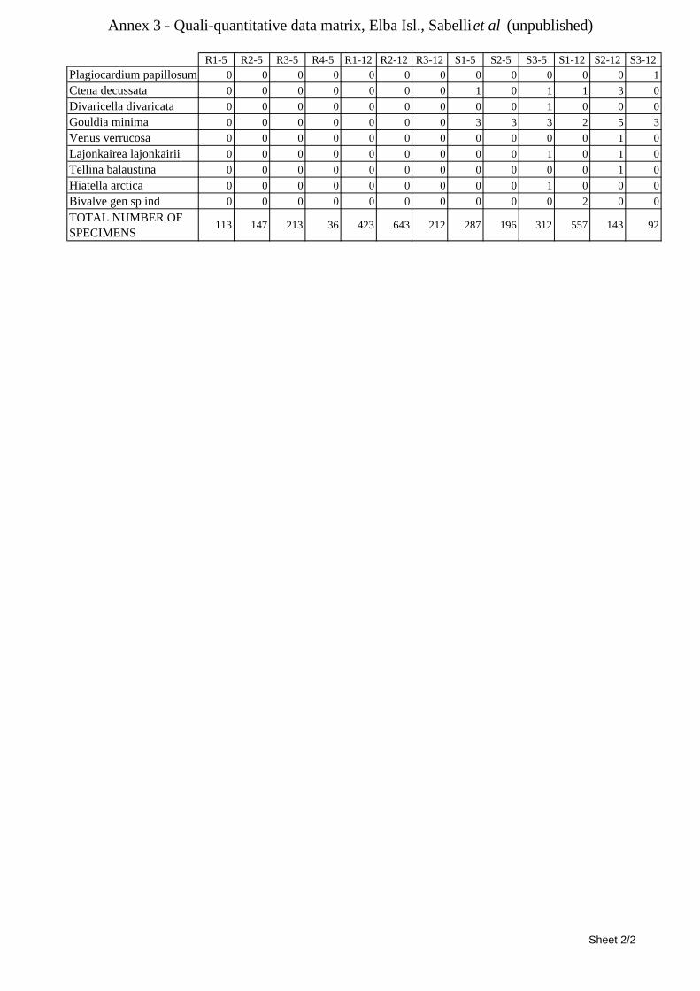
Annex 3 - Quali-quantitative data matrix, Elba Isl., Sabelli et al (unpublished)

R1-5 R2-5 R3-5 R4-5 R1-12 R2-12 R3-12 S1-5 S2-5 S3-5 S1-12 S2-12 S3-12Plagiocardium papillosum 0 0 0 0 0 0 0 0 0 0 0 0 1Ctena decussata 0 0 0 0 0 0 0 1 0 1 1 3 0Divaricella divaricata 0 0 0 0 0 0 0 0 0 1 0 0 0Gouldia minima 0 0 0 0 0 0 0 3 3 3 2 5 3Venus verrucosa 0 0 0 0 0 0 0 0 0 0 0 1 0Lajonkairea lajonkairii 0 0 0 0 0 0 0 0 0 1 0 1 0Tellina balaustina 0 0 0 0 0 0 0 0 0 0 0 1 0Hiatella arctica 0 0 0 0 0 0 0 0 0 1 0 0 0Bivalve gen sp ind 0 0 0 0 0 0 0 0 0 0 2 0 0TOTAL NUMBER OF SPECIMENS

113 147 213 36 423 643 212 287 196 312 557 143 92

Sheet 2/2

ANNEX 4

QUALI-QUANTITATIVE RESULTS OF THE SAMPLING IN POSIDONIA OCEANICA

IN GIGLIO ISLAND (BOTH LEAVES AND RHIZOMES,

BONFITTO ET AL., 1998)

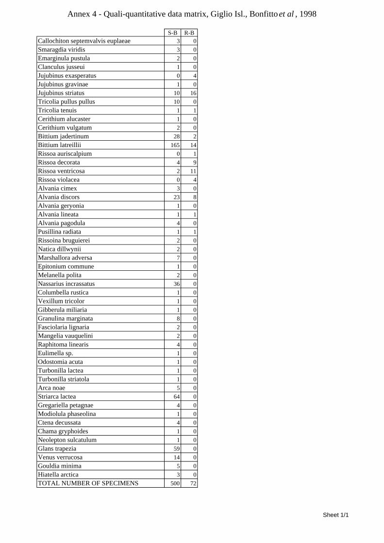
Annex 4 - Quali-quantitative data matrix, Giglio Isl., Bonfitto et al , 1998

S-B R-BCallochiton septemvalvis euplaeae 3 0Smaragdia viridis 3 0Emarginula pustula 2 0Clanculus jusseui 1 0Jujubinus exasperatus 0 4Jujubinus gravinae 1 0Jujubinus striatus 10 16Tricolia pullus pullus 10 0Tricolia tenuis 1 1Cerithium alucaster 1 0Cerithium vulgatum 2 0Bittium jadertinum 28 2Bittium latreillii 165 14Rissoa auriscalpium 0 1Rissoa decorata 4 9Rissoa ventricosa 2 11Rissoa violacea 0 4Alvania cimex 3 0Alvania discors 23 8Alvania geryonia 1 0Alvania lineata 1 1Alvania pagodula 4 0Pusillina radiata 1 1Rissoina bruguierei 2 0Natica dillwynii 2 0Marshallora adversa 7 0Epitonium commune 1 0Melanella polita 2 0Nassarius incrassatus 36 0Columbella rustica 1 0Vexillum tricolor 1 0Gibberula miliaria 1 0Granulina marginata 8 0Fasciolaria lignaria 2 0Mangelia vauquelini 2 0Raphitoma linearis 4 0Eulimella sp. 1 0Odostomia acuta 1 0Turbonilla lactea 1 0Turbonilla striatola 1 0Arca noae 5 0Striarca lactea 64 0Gregariella petagnae 4 0Modiolula phaseolina 1 0Ctena decussata 4 0Chama gryphoides 1 0Neolepton sulcatulum 1 0Glans trapezia 59 0Venus verrucosa 14 0Gouldia minima 5 0Hiatella arctica 3 0TOTAL NUMBER OF SPECIMENS 500 72

Sheet 1/1

ANNEX 5

QUALI-QUANTITATIVE RESULTS OF THE SAMPLING IN POSIDONIA OCEANICA

IN ISCHIA ISLAND (LEAVES STRATUM, IDATO ET AL., 1983)

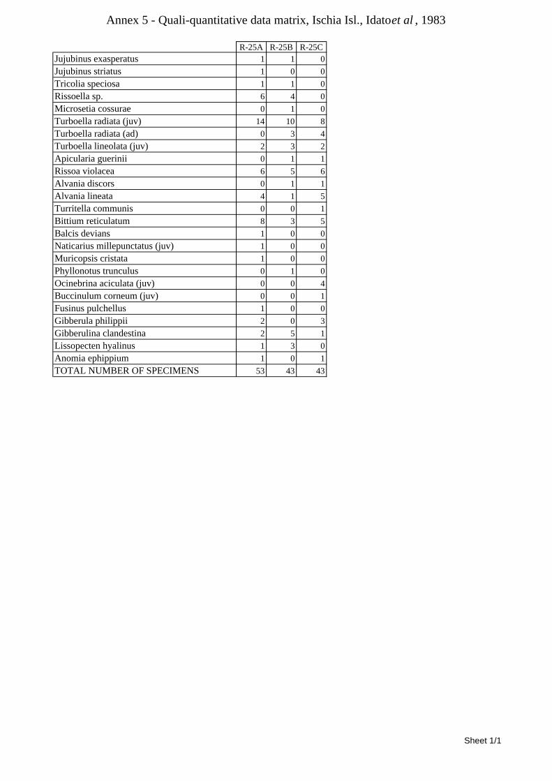
Annex 5 - Quali-quantitative data matrix, Ischia Isl., Idato et al , 1983

R-25A R-25B R-25CJujubinus exasperatus 1 1 0Jujubinus striatus 1 0 0Tricolia speciosa 1 1 0Rissoella sp. 6 4 0Microsetia cossurae 0 1 0Turboella radiata (juv) 14 10 8Turboella radiata (ad) 0 3 4Turboella lineolata (juv) 2 3 2Apicularia guerinii 0 1 1Rissoa violacea 6 5 6Alvania discors 0 1 1Alvania lineata 4 1 5Turritella communis 0 0 1Bittium reticulatum 8 3 5Balcis devians 1 0 0Naticarius millepunctatus (juv) 1 0 0Muricopsis cristata 1 0 0Phyllonotus trunculus 0 1 0Ocinebrina aciculata (juv) 0 0 4Buccinulum corneum (juv) 0 0 1Fusinus pulchellus 1 0 0Gibberula philippii 2 0 3Gibberulina clandestina 2 5 1Lissopecten hyalinus 1 3 0Anomia ephippium 1 0 1TOTAL NUMBER OF SPECIMENS 53 43 43

Sheet 1/1

ANNEX 6

QUALI-QUANTITATIVE RESULTS OF THE SAMPLING IN POSIDONIA OCEANICA

IN HVRGADA ISLAND, CROATIA (BOTH LEAVES AND RHIZOMES,

SOLUSTRI ET AL., 2002)

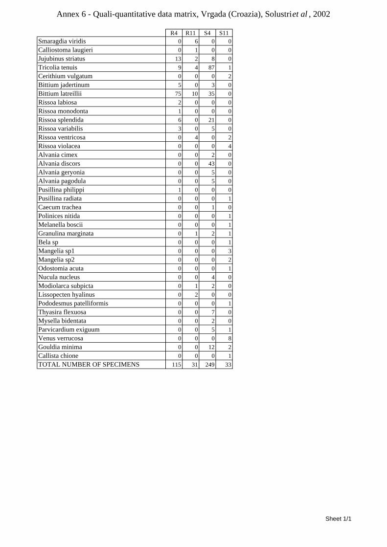
Annex 6 - Quali-quantitative data matrix, Vrgada (Croazia), Solustri et al , 2002

R4 R11 S4 S11Smaragdia viridis 0 6 0 0Calliostoma laugieri 0 1 0 0Jujubinus striatus 13 2 8 0Tricolia tenuis 9 4 87 1Cerithium vulgatum 0 0 0 2Bittium jadertinum 5 0 3 0Bittium latreillii 75 10 35 0Rissoa labiosa 2 0 0 0Rissoa monodonta 1 0 0 0Rissoa splendida 6 0 21 0Rissoa variabilis 3 0 5 0Rissoa ventricosa 0 4 0 2Rissoa violacea 0 0 0 4Alvania cimex 0 0 2 0Alvania discors 0 0 43 0Alvania geryonia 0 0 5 0Alvania pagodula 0 0 5 0Pusillina philippi 1 0 0 0Pusillina radiata 0 0 0 1Caecum trachea 0 0 1 0Polinices nitida 0 0 0 1Melanella boscii 0 0 0 1Granulina marginata 0 1 2 1Bela sp 0 0 0 1Mangelia sp1 0 0 0 3Mangelia sp2 0 0 0 2Odostomia acuta 0 0 0 1Nucula nucleus 0 0 4 0Modiolarca subpicta 0 1 2 0Lissopecten hyalinus 0 2 0 0Pododesmus patelliformis 0 0 0 1Thyasira flexuosa 0 0 7 0Mysella bidentata 0 0 2 0Parvicardium exiguum 0 0 5 1Venus verrucosa 0 0 0 8Gouldia minima 0 0 12 2Callista chione 0 0 0 1TOTAL NUMBER OF SPECIMENS 115 31 249 33

Sheet 1/1

ANNEX 7

QUALI-QUANTITATIVE RESULTS OF THE SAMPLING IN THE CORALLIGENOUS

IN SECCHE DI TOR PATERNO (UNIVERSITÀ LA SAPIENZA, 1993)

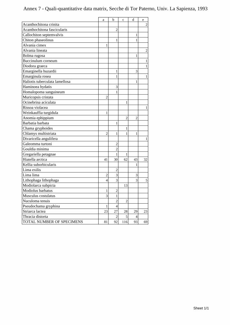
Annex 7 - Quali-quantitative data matrix, Secche di Tor Paterno, Univ. La Sapienza, 1993

a b c d eAcanthochitona crinita 2Acanthochitona fascicularis 2Callochiton septemvalvis 1Chiton phaseolinus 1 1Alvania cimex 1Alvania lineata 2Bolma rugosa 1Buccinulum corneum 1Diodora graeca 1Emarginella huzardii 1 3Emarginula rosea 1 1Haliotis tuberculata lamellosa 1Haminoea hydatis 3Homalopoma sanguineum 1Muricopsis cristata 2Ocinebrina aciculata 1Rissoa violacea 1Weinkauffia turgidula 1Anomia ephippium 2 2Barbatia barbata 1Chama gryphoides 1Chlamys multistriata 2 1 1 1Divaricella angulifera 1Galeomma turtoni 2Gouldia minima 2Gregariella petagnae 1 1Hiatella arctica 41 30 62 43 32Kellia suborbicularis 1Lima exilis 2Lima lima 2 3 3Lithophaga lithophaga 4 3 3 5Modiolarca subpicta 13Modiolus barbatus 1 2Musculus costulatus 3 1Nuculoma tenuis 2 2Pseudochama gryphina 1 4Striarca lactea 23 27 28 29 23Thracia distorta 2 5 4TOTAL NUMBER OF SPECIMENS 81 92 116 93 69

Sheet 1/1

ANNEX 8

QUALI-QUANTITATIVE RESULTS OF THE SAMPLING IN THE CORALLIGENOUS

IN SCIACCA (SICILY) (GILLONE, 1990)

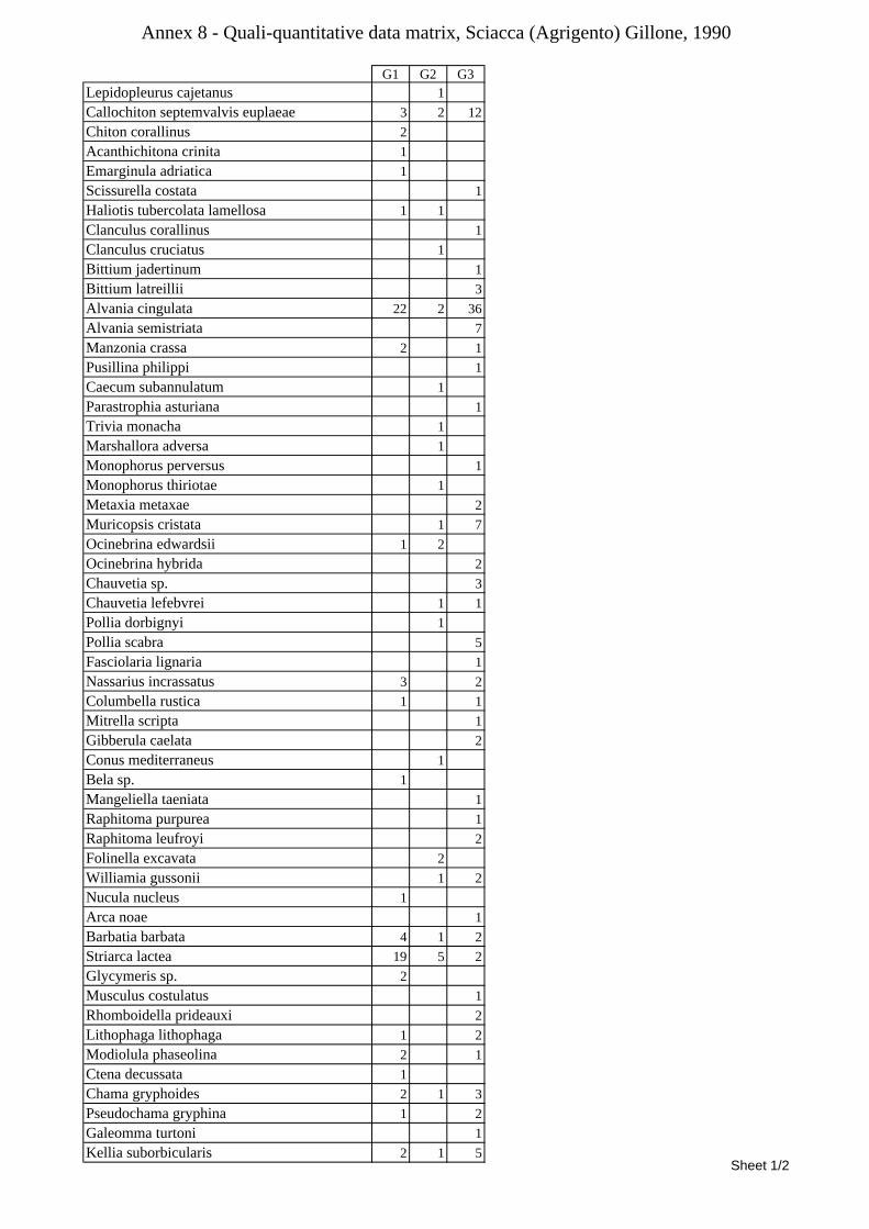
Annex 8 - Quali-quantitative data matrix, Sciacca (Agrigento) Gillone, 1990

G1 G2 G3Lepidopleurus cajetanus 1Callochiton septemvalvis euplaeae 3 2 12Chiton corallinus 2Acanthichitona crinita 1Emarginula adriatica 1Scissurella costata 1Haliotis tubercolata lamellosa 1 1Clanculus corallinus 1Clanculus cruciatus 1Bittium jadertinum 1Bittium latreillii 3Alvania cingulata 22 2 36Alvania semistriata 7Manzonia crassa 2 1Pusillina philippi 1Caecum subannulatum 1Parastrophia asturiana 1Trivia monacha 1Marshallora adversa 1Monophorus perversus 1Monophorus thiriotae 1Metaxia metaxae 2Muricopsis cristata 1 7Ocinebrina edwardsii 1 2Ocinebrina hybrida 2Chauvetia sp. 3Chauvetia lefebvrei 1 1Pollia dorbignyi 1Pollia scabra 5Fasciolaria lignaria 1Nassarius incrassatus 3 2Columbella rustica 1 1Mitrella scripta 1Gibberula caelata 2Conus mediterraneus 1Bela sp. 1Mangeliella taeniata 1Raphitoma purpurea 1Raphitoma leufroyi 2Folinella excavata 2Williamia gussonii 1 2Nucula nucleus 1Arca noae 1Barbatia barbata 4 1 2Striarca lactea 19 5 2Glycymeris sp. 2Musculus costulatus 1Rhomboidella prideauxi 2Lithophaga lithophaga 1 2Modiolula phaseolina 2 1Ctena decussata 1Chama gryphoides 2 1 3Pseudochama gryphina 1 2Galeomma turtoni 1Kellia suborbicularis 2 1 5

Sheet 1/2

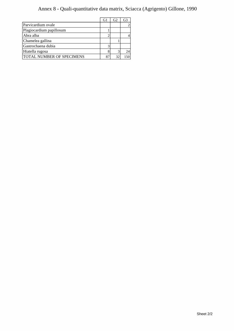
Annex 8 - Quali-quantitative data matrix, Sciacca (Agrigento) Gillone, 1990

G1 G2 G3Parvicardium ovale 2Plagiocardium papillosum 1Abra alba 2 4Chamelea gallina 1Gastrochaena dubia 3Hiatella rugosa 8 3 24TOTAL NUMBER OF SPECIMENS 87 32 150

Sheet 2/2

ANNEX 9

QUALI-QUANTITATIVE RESULTS OF THE SAMPLING IN THE CORALLIGENOUS

IN SCOPELLO (SICILY) (GILLONE, 1990)

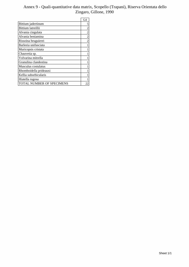
Annex 9 - Quali-quantitative data matrix, Scopello (Trapani), Riserva Orientata dello Zingaro, Gillone, 1990

G4Bittium jadertinum 5Bittium latreillii 2Alvania cingulata 2Alvania beniamina 2Rissoina bruguierei 2Barleeia unifasciata 1Muricopsis cristata 1Chauvetia sp. 1Volvarina mitrella 1Granulina clandestina 1Musculus costulatus 1Rhomboidella prideauxi 1Kellia suborbicularis 1Hiatella rugosa 1TOTAL NUMBER OF SPECIMENS 22

Sheet 1/1

ANNEX 10

QUALI-QUANTITATIVE RESULTS OF THE SAMPLING IN THE SOFT SUBSTRATA

AROUND SECCHE DI TOR PATERNO (UNIVERSITÀ TOR VERGATA, 2005)

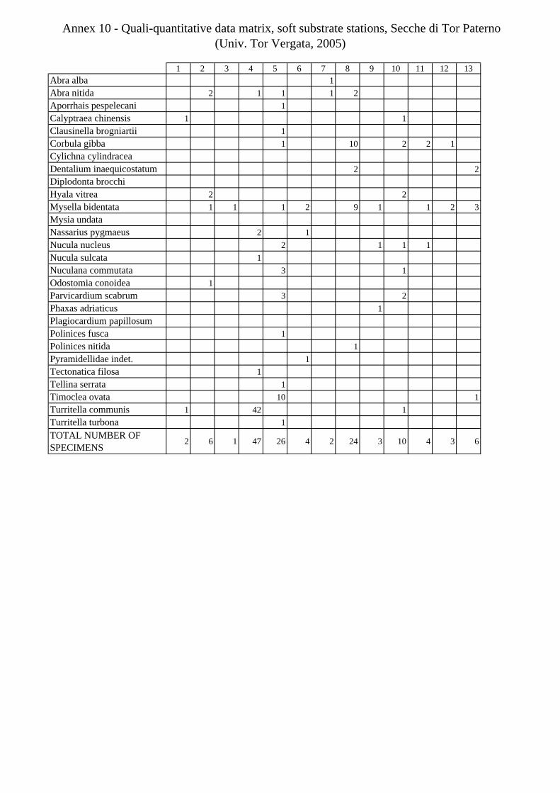
Annex 10 - Quali-quantitative data matrix, soft substrate stations, Secche di Tor Paterno (Univ. Tor Vergata, 2005)

1 2 3 4 5 6 7 8 9 10 11 12 13Abra alba 1Abra nitida 2 1 1 1 2Aporrhais pespelecani 1Calyptraea chinensis 1 1Clausinella brogniartii 1Corbula gibba 1 10 2 2 1Cylichna cylindraceaDentalium inaequicostatum 2 2Diplodonta brocchiHyala vitrea 2 2Mysella bidentata 1 1 1 2 9 1 1 2 3Mysia undataNassarius pygmaeus 2 1Nucula nucleus 2 1 1 1Nucula sulcata 1Nuculana commutata 3 1Odostomia conoidea 1Parvicardium scabrum 3 2Phaxas adriaticus 1Plagiocardium papillosumPolinices fusca 1Polinices nitida 1Pyramidellidae indet. 1Tectonatica filosa 1Tellina serrata 1Timoclea ovata 10 1Turritella communis 1 42 1Turritella turbona 1TOTAL NUMBER OF SPECIMENS

2 6 1 47 26 4 2 24 3 10 4 3 6

Annex 10 - Quali-quantitative data matrix, soft substrate stations, Secche di Tor Paterno (Univ. Tor Vergata, 2005)

Abra albaAbra nitidaAporrhais pespelecaniCalyptraea chinensisClausinella brogniartiiCorbula gibbaCylichna cylindraceaDentalium inaequicostatumDiplodonta brocchiHyala vitreaMysella bidentataMysia undataNassarius pygmaeusNucula nucleusNucula sulcataNuculana commutataOdostomia conoideaParvicardium scabrumPhaxas adriaticusPlagiocardium papillosumPolinices fuscaPolinices nitidaPyramidellidae indet.Tectonatica filosaTellina serrataTimoclea ovataTurritella communisTurritella turbonaTOTAL NUMBER OF SPECIMENS

14 15 16 17 18 19 20 21 22 23 24 25 261 2

2 1 2 2 4 1

1

1 2 4 11

4 1 1 11 1 1

2 22 2 7 1

11

2 1 11

11 1 1 1 1 1

1

1

11

3

4 6 10 12 9 1 2 2 11 2 4 7 2

ANNEX 11

QUALI-QUANTITATIVE RESULTS OF THE PLEOCYEMATA (CRUSTACEA) SAMPLED

IN SECCHE DI TOR PATERNO

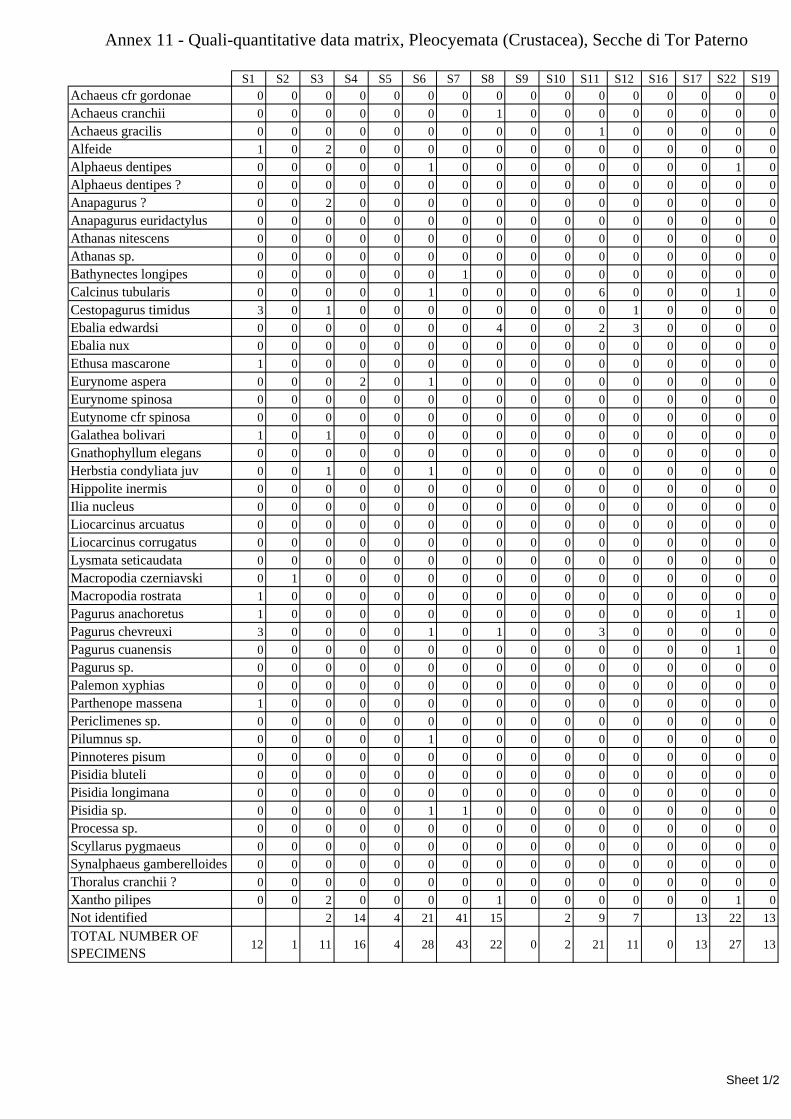
Annex 11 - Quali-quantitative data matrix, Pleocyemata (Crustacea), Secche di Tor Paterno

S1 S2 S3 S4 S5 S6 S7 S8 S9 S10 S11 S12 S16 S17 S22 S19Achaeus cfr gordonae 0 0 0 0 0 0 0 0 0 0 0 0 0 0 0 0Achaeus cranchii 0 0 0 0 0 0 0 1 0 0 0 0 0 0 0 0Achaeus gracilis 0 0 0 0 0 0 0 0 0 0 1 0 0 0 0 0Alfeide 1 0 2 0 0 0 0 0 0 0 0 0 0 0 0 0Alphaeus dentipes 0 0 0 0 0 1 0 0 0 0 0 0 0 0 1 0Alphaeus dentipes ? 0 0 0 0 0 0 0 0 0 0 0 0 0 0 0 0Anapagurus ? 0 0 2 0 0 0 0 0 0 0 0 0 0 0 0 0Anapagurus euridactylus 0 0 0 0 0 0 0 0 0 0 0 0 0 0 0 0Athanas nitescens 0 0 0 0 0 0 0 0 0 0 0 0 0 0 0 0Athanas sp. 0 0 0 0 0 0 0 0 0 0 0 0 0 0 0 0Bathynectes longipes 0 0 0 0 0 0 1 0 0 0 0 0 0 0 0 0Calcinus tubularis 0 0 0 0 0 1 0 0 0 0 6 0 0 0 1 0Cestopagurus timidus 3 0 1 0 0 0 0 0 0 0 0 1 0 0 0 0Ebalia edwardsi 0 0 0 0 0 0 0 4 0 0 2 3 0 0 0 0Ebalia nux 0 0 0 0 0 0 0 0 0 0 0 0 0 0 0 0Ethusa mascarone 1 0 0 0 0 0 0 0 0 0 0 0 0 0 0 0Eurynome aspera 0 0 0 2 0 1 0 0 0 0 0 0 0 0 0 0Eurynome spinosa 0 0 0 0 0 0 0 0 0 0 0 0 0 0 0 0Eutynome cfr spinosa 0 0 0 0 0 0 0 0 0 0 0 0 0 0 0 0Galathea bolivari 1 0 1 0 0 0 0 0 0 0 0 0 0 0 0 0Gnathophyllum elegans 0 0 0 0 0 0 0 0 0 0 0 0 0 0 0 0Herbstia condyliata juv 0 0 1 0 0 1 0 0 0 0 0 0 0 0 0 0Hippolite inermis 0 0 0 0 0 0 0 0 0 0 0 0 0 0 0 0Ilia nucleus 0 0 0 0 0 0 0 0 0 0 0 0 0 0 0 0Liocarcinus arcuatus 0 0 0 0 0 0 0 0 0 0 0 0 0 0 0 0Liocarcinus corrugatus 0 0 0 0 0 0 0 0 0 0 0 0 0 0 0 0Lysmata seticaudata 0 0 0 0 0 0 0 0 0 0 0 0 0 0 0 0Macropodia czerniavski 0 1 0 0 0 0 0 0 0 0 0 0 0 0 0 0Macropodia rostrata 1 0 0 0 0 0 0 0 0 0 0 0 0 0 0 0Pagurus anachoretus 1 0 0 0 0 0 0 0 0 0 0 0 0 0 1 0Pagurus chevreuxi 3 0 0 0 0 1 0 1 0 0 3 0 0 0 0 0Pagurus cuanensis 0 0 0 0 0 0 0 0 0 0 0 0 0 0 1 0Pagurus sp. 0 0 0 0 0 0 0 0 0 0 0 0 0 0 0 0Palemon xyphias 0 0 0 0 0 0 0 0 0 0 0 0 0 0 0 0Parthenope massena 1 0 0 0 0 0 0 0 0 0 0 0 0 0 0 0Periclimenes sp. 0 0 0 0 0 0 0 0 0 0 0 0 0 0 0 0Pilumnus sp. 0 0 0 0 0 1 0 0 0 0 0 0 0 0 0 0Pinnoteres pisum 0 0 0 0 0 0 0 0 0 0 0 0 0 0 0 0Pisidia bluteli 0 0 0 0 0 0 0 0 0 0 0 0 0 0 0 0Pisidia longimana 0 0 0 0 0 0 0 0 0 0 0 0 0 0 0 0Pisidia sp. 0 0 0 0 0 1 1 0 0 0 0 0 0 0 0 0Processa sp. 0 0 0 0 0 0 0 0 0 0 0 0 0 0 0 0Scyllarus pygmaeus 0 0 0 0 0 0 0 0 0 0 0 0 0 0 0 0Synalphaeus gamberelloides 0 0 0 0 0 0 0 0 0 0 0 0 0 0 0 0Thoralus cranchii ? 0 0 0 0 0 0 0 0 0 0 0 0 0 0 0 0Xantho pilipes 0 0 2 0 0 0 0 1 0 0 0 0 0 0 1 0Not identified 2 14 4 21 41 15 2 9 7 13 22 13TOTAL NUMBER OF SPECIMENS

12 1 11 16 4 28 43 22 0 2 21 11 0 13 27 13

Sheet 1/2

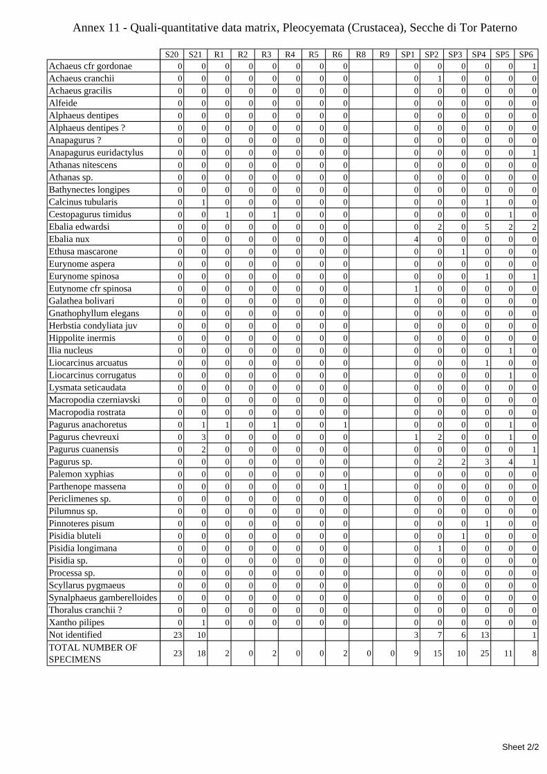
Annex 11 - Quali-quantitative data matrix, Pleocyemata (Crustacea), Secche di Tor Paterno

Achaeus cfr gordonaeAchaeus cranchii Achaeus gracilisAlfeideAlphaeus dentipes Alphaeus dentipes ?Anapagurus ?Anapagurus euridactylusAthanas nitescensAthanas sp.Bathynectes longipesCalcinus tubularisCestopagurus timidusEbalia edwardsiEbalia nuxEthusa mascaroneEurynome asperaEurynome spinosaEutynome cfr spinosaGalathea bolivariGnathophyllum elegansHerbstia condyliata juvHippolite inermisIlia nucleusLiocarcinus arcuatusLiocarcinus corrugatusLysmata seticaudataMacropodia czerniavskiMacropodia rostrataPagurus anachoretusPagurus chevreuxiPagurus cuanensisPagurus sp.Palemon xyphiasParthenope massenaPericlimenes sp.Pilumnus sp.Pinnoteres pisumPisidia bluteliPisidia longimanaPisidia sp.Processa sp.Scyllarus pygmaeusSynalphaeus gamberelloidesThoralus cranchii ?Xantho pilipesNot identifiedTOTAL NUMBER OF SPECIMENS

S20 S21 R1 R2 R3 R4 R5 R6 R8 R9 SP1 SP2 SP3 SP4 SP5 SP60 0 0 0 0 0 0 0 0 0 0 0 0 10 0 0 0 0 0 0 0 0 1 0 0 0 00 0 0 0 0 0 0 0 0 0 0 0 0 00 0 0 0 0 0 0 0 0 0 0 0 0 00 0 0 0 0 0 0 0 0 0 0 0 0 00 0 0 0 0 0 0 0 0 0 0 0 0 00 0 0 0 0 0 0 0 0 0 0 0 0 00 0 0 0 0 0 0 0 0 0 0 0 0 10 0 0 0 0 0 0 0 0 0 0 0 0 00 0 0 0 0 0 0 0 0 0 0 0 0 00 0 0 0 0 0 0 0 0 0 0 0 0 00 1 0 0 0 0 0 0 0 0 0 1 0 00 0 1 0 1 0 0 0 0 0 0 0 1 00 0 0 0 0 0 0 0 0 2 0 5 2 20 0 0 0 0 0 0 0 4 0 0 0 0 00 0 0 0 0 0 0 0 0 0 1 0 0 00 0 0 0 0 0 0 0 0 0 0 0 0 00 0 0 0 0 0 0 0 0 0 0 1 0 10 0 0 0 0 0 0 0 1 0 0 0 0 00 0 0 0 0 0 0 0 0 0 0 0 0 00 0 0 0 0 0 0 0 0 0 0 0 0 00 0 0 0 0 0 0 0 0 0 0 0 0 00 0 0 0 0 0 0 0 0 0 0 0 0 00 0 0 0 0 0 0 0 0 0 0 0 1 00 0 0 0 0 0 0 0 0 0 0 1 0 00 0 0 0 0 0 0 0 0 0 0 0 1 00 0 0 0 0 0 0 0 0 0 0 0 0 00 0 0 0 0 0 0 0 0 0 0 0 0 00 0 0 0 0 0 0 0 0 0 0 0 0 00 1 1 0 1 0 0 1 0 0 0 0 1 00 3 0 0 0 0 0 0 1 2 0 0 1 00 2 0 0 0 0 0 0 0 0 0 0 0 10 0 0 0 0 0 0 0 0 2 2 3 4 10 0 0 0 0 0 0 0 0 0 0 0 0 00 0 0 0 0 0 0 1 0 0 0 0 0 00 0 0 0 0 0 0 0 0 0 0 0 0 00 0 0 0 0 0 0 0 0 0 0 0 0 00 0 0 0 0 0 0 0 0 0 0 1 0 00 0 0 0 0 0 0 0 0 0 1 0 0 00 0 0 0 0 0 0 0 0 1 0 0 0 00 0 0 0 0 0 0 0 0 0 0 0 0 00 0 0 0 0 0 0 0 0 0 0 0 0 00 0 0 0 0 0 0 0 0 0 0 0 0 00 0 0 0 0 0 0 0 0 0 0 0 0 00 0 0 0 0 0 0 0 0 0 0 0 0 00 1 0 0 0 0 0 0 0 0 0 0 0 0

23 10 3 7 6 13 1

23 18 2 0 2 0 0 2 0 0 9 15 10 25 11 8

Sheet 2/2

ANNEX 12

QUALI-QUANTITATIVE RESULTS OF THE ERRANT POLYCHAETA SAMPLED

IN SECCHE DI TOR PATERNO

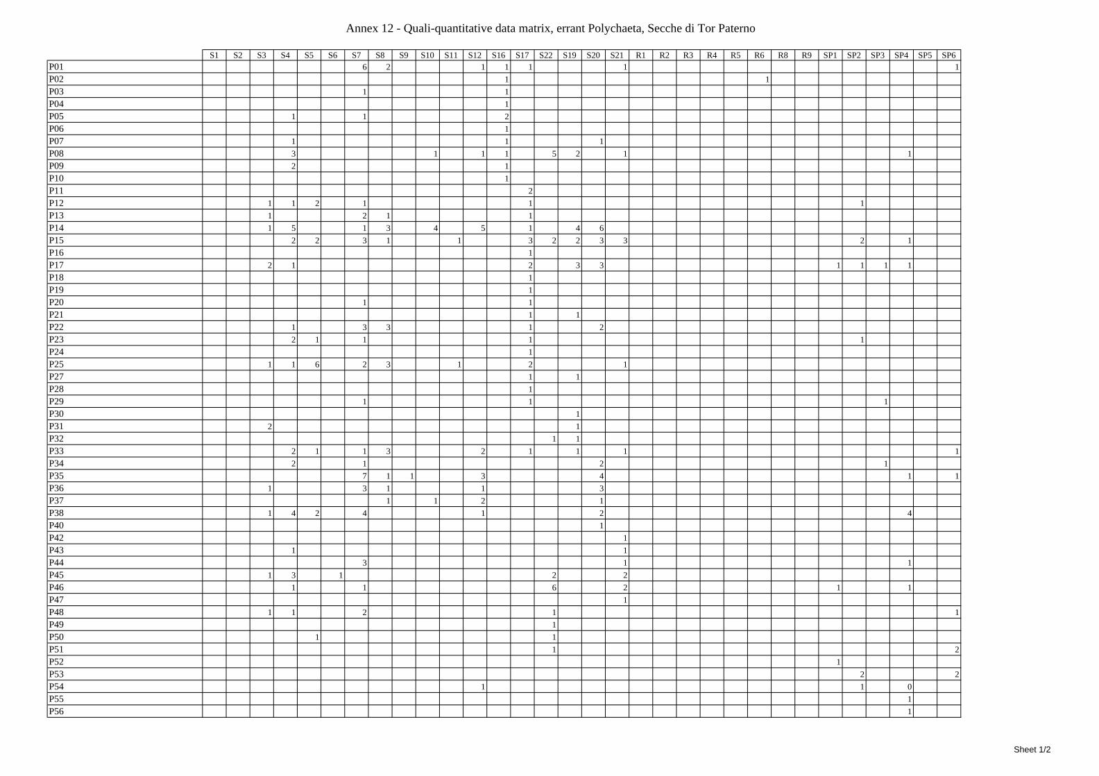
Annex 12 - Quali-quantitative data matrix, errant Polychaeta, Secche di Tor Paterno

S1 S2 S3 S4 S5 S6 S7 S8 S9 S10 S11 S12 S16 S17 S22 S19 S20 S21 R1 R2 R3 R4 R5 R6 R8 R9 SP1 SP2 SP3 SP4 SP5 SP6P01 6 2 1 1 1 1 1P02 1 1P03 1 1P04 1P05 1 1 2P06 1P07 1 1 1P08 3 1 1 1 5 2 1 1P09 2 1P10 1P11 2P12 1 1 2 1 1 1P13 1 2 1 1P14 1 5 1 3 4 5 1 4 6P15 2 2 3 1 1 3 2 2 3 3 2 1P16 1P17 2 1 2 3 3 1 1 1 1P18 1P19 1P20 1 1P21 1 1P22 1 3 3 1 2P23 2 1 1 1 1P24 1P25 1 1 6 2 3 1 2 1P27 1 1P28 1P29 1 1 1P30 1P31 2 1P32 1 1P33 2 1 1 3 2 1 1 1 1P34 2 1 2 1P35 7 1 1 3 4 1 1P36 1 3 1 1 3P37 1 1 2 1P38 1 4 2 4 1 2 4P40 1P42 1P43 1 1P44 3 1 1P45 1 3 1 2 2P46 1 1 6 2 1 1P47 1P48 1 1 2 1 1P49 1P50 1 1P51 1 2P52 1P53 2 2P54 1 1 0P55 1P56 1

Sheet 1/2

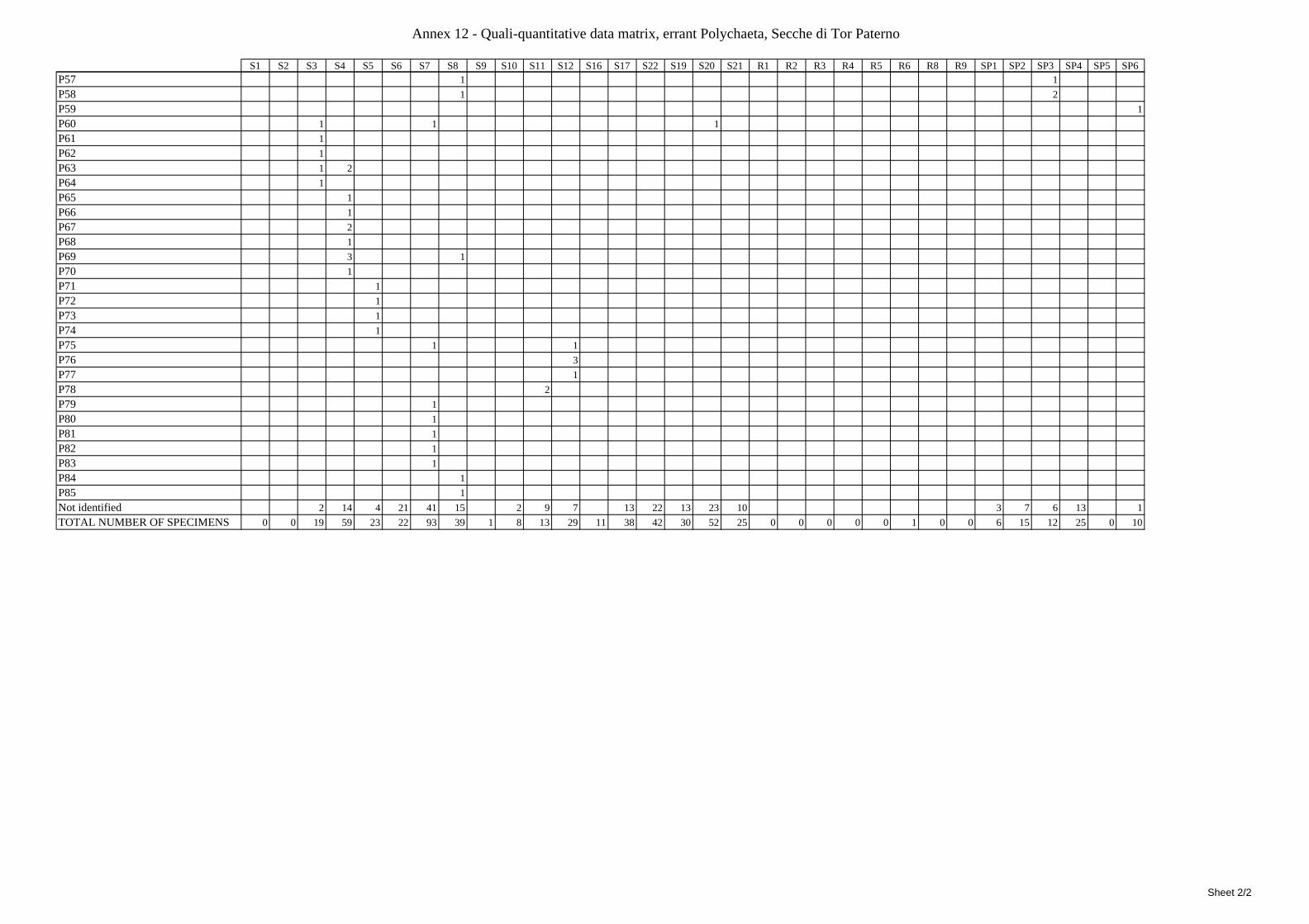
Annex 12 - Quali-quantitative data matrix, errant Polychaeta, Secche di Tor Paterno

S1 S2 S3 S4 S5 S6 S7 S8 S9 S10 S11 S12 S16 S17 S22 S19 S20 S21 R1 R2 R3 R4 R5 R6 R8 R9 SP1 SP2 SP3 SP4 SP5 SP6P57 1 1P58 1 2P59 1P60 1 1 1P61 1P62 1P63 1 2P64 1P65 1P66 1P67 2P68 1P69 3 1P70 1P71 1P72 1P73 1P74 1P75 1 1P76 3P77 1P78 2P79 1P80 1P81 1P82 1P83 1P84 1P85 1Not identified 2 14 4 21 41 15 2 9 7 13 22 13 23 10 3 7 6 13 1TOTAL NUMBER OF SPECIMENS 0 0 19 59 23 22 93 39 1 8 13 29 11 38 42 30 52 25 0 0 0 0 0 1 0 0 6 15 12 25 0 10

Sheet 2/2

ANNEX 13

QUALI-QUANTITATIVE RESULTS OF THE MOLLUSCS SAMPLED

IN SECCHE DI TOR PATERNO SIZE RANGE 1-6 MM FOR LIVE-DEAD

COMPARISON

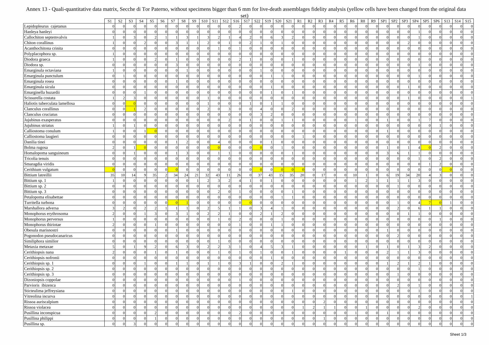
Annex 13 - Quali-quantitative data matrix, Secche di Tor Paterno, without specimens bigger than 6 mm for live-death assemblages fidelity analysis (yellow cells have been changed from the original data set)

S1 S2 S3 S4 S5 S6 S7 S8 S9 S10 S11 S12 S16 S17 S22 S19 S20 S21 R1 R2 R3 R4 R5 R6 R8 R9 SP1 SP2 SP3 SP4 SP5 SP6 S13 S14 S15Lepidopleurus cajetanus 0 0 0 0 0 0 0 0 0 0 0 0 2 0 0 0 0 0 0 0 0 0 0 0 0 0 0 0 0 0 0 0 0 0 0Hanleya hanleyi 0 0 0 0 0 0 0 0 0 0 0 0 0 0 0 0 0 0 0 0 0 0 0 0 0 0 0 0 0 1 0 0 0 0 0Callochiton septemvalvis 1 0 3 0 2 1 1 3 1 3 2 1 4 2 0 6 3 2 0 0 0 0 0 0 0 0 0 0 0 1 0 0 0 0 0Chiton corallinus 1 0 0 2 0 0 3 1 1 2 0 1 0 2 1 0 1 0 0 0 0 0 0 0 0 0 0 0 2 0 0 0 0 0 0Acanthochitona crinita 0 0 0 0 0 0 0 0 0 0 1 0 1 0 0 0 0 0 0 0 0 0 0 0 0 0 0 0 0 0 0 0 0 0 0Polyplacophora sp. 1 0 0 0 0 0 0 0 0 0 0 0 0 0 0 0 0 0 0 0 0 0 0 0 0 0 0 0 0 0 0 0 0 0 0Diodora graeca 1 0 0 0 2 0 1 0 0 0 0 0 2 1 0 0 0 1 0 0 0 0 0 0 0 0 0 0 0 0 0 0 0 0 0Diodora sp. 0 0 0 0 0 0 3 0 0 0 0 0 0 0 0 0 0 0 0 0 0 0 0 0 0 0 0 0 0 1 0 0 0 0 0Emarginula octaviana 1 0 0 0 0 0 0 1 0 0 0 0 0 0 1 0 0 0 0 0 0 0 0 0 0 0 0 0 0 0 0 0 0 0 0Emarginula punctulum 0 1 0 0 0 0 0 0 0 0 0 0 0 0 0 1 1 0 0 0 0 0 0 0 0 0 0 0 0 1 0 0 0 0 0Emarginula rosea 0 0 0 0 0 0 1 0 0 0 0 0 0 0 0 0 0 0 0 0 0 0 0 0 0 0 0 0 0 0 0 0 0 0 0Emarginula sicula 0 0 0 0 0 0 0 0 0 0 0 0 0 0 0 1 0 0 0 0 0 0 0 0 0 0 0 0 1 0 0 0 0 0 0Emarginella huzardii 0 0 0 1 0 0 0 0 0 0 0 0 0 0 0 1 0 1 0 0 0 0 0 0 0 0 0 0 0 0 0 0 0 0 0Scissurella costata 1 2 3 0 0 0 0 0 0 1 0 0 0 0 0 0 0 0 0 0 0 0 0 0 0 0 0 0 1 0 0 0 0 0 1Haliotis tuberculata lamellosa 0 0 0 0 0 0 0 0 0 1 0 0 0 1 0 1 1 0 0 0 0 0 0 0 0 0 0 0 0 0 0 0 0 0 0Clanculus corallinus 0 0 1 2 0 0 0 0 0 2 0 3 0 0 4 0 0 2 0 0 0 0 0 0 0 0 0 0 0 0 0 0 0 0 0Clanculus cruciatus 0 0 0 0 0 0 0 0 0 0 0 0 0 0 3 2 0 0 0 0 0 0 0 0 0 0 0 0 0 0 0 0 0 0 0Jujubinus exasperatus 0 0 0 0 0 0 0 0 0 0 0 2 0 1 0 0 1 1 0 0 0 0 0 1 0 0 1 0 0 1 7 0 0 0 0Jujubinus striatus 1 0 1 0 0 0 0 0 0 0 0 0 0 0 0 0 0 0 0 0 0 0 0 0 0 0 0 0 0 0 0 1 0 0 0Calliostoma conulum 1 0 0 1 0 0 0 0 0 0 0 0 0 0 0 0 0 0 0 0 0 0 0 0 0 0 1 0 0 0 0 0 0 0 0Calliostoma laugieri 0 0 0 0 0 0 0 0 0 0 0 0 0 0 0 0 0 0 1 0 0 0 0 0 0 0 0 0 0 0 0 0 0 0 0Danilia tinei 0 0 0 0 0 0 1 2 0 0 4 0 0 0 0 1 0 0 0 0 0 0 0 0 0 0 0 0 0 0 0 0 0 0 0Bolma rugosa 2 0 1 0 0 0 0 0 0 0 0 0 0 0 0 0 1 0 0 0 0 0 0 0 0 0 1 0 1 4 0 2 0 0 0Homalopoma sanguineum 0 0 1 0 0 0 1 3 0 0 1 1 0 0 0 0 0 1 0 0 0 0 0 0 0 0 3 6 1 1 0 0 0 0 0Tricolia tenuis 0 0 0 0 0 0 0 0 0 0 0 0 0 0 0 0 0 0 0 0 0 0 0 0 0 0 0 0 0 1 0 2 0 0 0Smaragdia viridis 0 0 0 0 0 0 0 0 0 0 0 0 0 0 0 0 0 0 0 0 0 0 0 0 0 0 0 0 0 0 1 2 0 0 0Cerithium vulgatum 0 0 0 0 0 0 0 0 0 0 0 0 0 0 0 0 0 0 0 0 0 0 0 0 0 0 0 0 0 0 0 0 0 0 0Bittium latreillii 35 10 14 9 35 2 34 24 21 32 43 11 26 0 37 43 15 35 20 0 17 0 0 10 1 0 6 19 34 20 4 3 0 0 0Bittium sp. 1 1 0 0 0 0 0 0 0 1 2 3 2 4 1 0 1 0 0 0 0 0 0 0 1 2 1 1 1 1 3 0 0 0 0 0Bittium sp. 2 0 0 0 0 0 0 0 0 0 0 0 0 0 0 0 0 0 0 0 0 0 0 0 0 0 0 0 1 0 0 0 0 0 0 0Bittium sp. 3 0 0 0 0 0 0 0 0 0 0 2 0 1 0 0 0 0 1 0 0 0 0 0 0 0 0 0 0 0 0 0 0 0 0 0Petalopoma elisabettae 0 0 0 0 0 0 0 0 0 0 0 0 0 0 0 0 1 1 0 0 0 0 0 0 0 0 0 0 0 0 0 0 0 0 0Turritella turbona 0 0 0 0 0 0 0 1 0 0 0 0 0 0 0 0 0 0 0 0 0 0 0 0 0 0 0 1 0 4 7 0 1 0 0Marshallora adversa 3 2 0 2 2 1 1 1 0 2 5 1 1 0 3 4 1 0 0 0 0 0 0 0 0 0 0 2 0 6 1 1 0 0 0Monophorus erythrosoma 2 0 0 1 3 0 3 1 0 2 2 1 0 0 2 1 2 0 0 0 0 0 0 0 0 0 0 0 1 1 0 0 0 0 0Monophorus perversus 1 0 0 0 0 0 0 0 0 0 1 0 2 0 0 0 1 0 0 0 0 0 0 0 0 0 0 0 0 0 0 1 0 0 0Monophorus thiriotae 2 0 0 0 1 0 0 0 0 0 0 0 1 0 0 1 1 0 0 0 0 0 0 0 0 0 0 0 0 0 0 0 0 0 0Obesula marisnostri 0 0 0 0 0 0 1 0 0 0 0 0 0 0 0 0 0 0 0 0 0 0 0 0 0 0 1 0 0 0 0 0 0 0 0Pogonodon pseudocanaricus 0 0 0 0 0 0 0 0 0 0 0 0 0 0 0 0 0 0 0 0 0 0 0 0 0 0 0 2 0 0 0 0 0 0 0Similiphora similior 0 0 0 0 0 0 0 0 0 0 1 0 0 0 0 0 0 0 0 0 0 0 0 0 0 0 0 0 0 0 0 0 0 0 0Metaxia metaxae 5 0 1 9 2 0 6 3 0 2 2 3 1 0 4 5 3 1 0 0 0 0 0 0 1 0 1 0 1 3 2 0 0 0 0Cerithiopsis nana 2 0 0 0 1 0 1 0 0 0 1 0 1 0 1 0 0 1 0 0 0 0 1 0 0 0 2 1 1 3 0 0 0 0 0Cerithiopsis nofronii 0 0 0 0 0 0 0 0 0 0 0 0 0 0 0 1 0 0 0 0 0 0 0 0 0 0 0 0 0 0 0 0 0 0 0Cerithiopsis sp. 1 0 0 0 1 0 0 1 1 0 1 1 0 3 1 0 0 2 1 0 0 0 0 0 0 0 0 1 2 1 2 1 0 0 0 0Cerithiopsis sp. 2 0 0 0 0 0 0 0 0 0 0 0 0 0 0 0 0 0 0 0 0 0 0 0 0 0 0 0 0 0 1 0 0 0 0 0Cerithiopsis sp. 3 0 0 0 0 0 0 0 0 0 0 0 0 0 0 0 0 0 0 0 0 0 0 0 0 0 0 0 1 0 0 0 0 0 0 0Dizoniopsis coppolae 0 0 0 0 0 0 0 0 0 0 0 0 1 0 0 0 0 0 0 0 0 0 0 0 0 0 0 0 0 0 0 0 0 0 0Parvioris ibizenca 0 0 0 0 0 0 0 0 0 0 0 0 0 0 0 0 0 0 0 0 0 0 0 0 0 0 0 2 0 1 0 0 0 0 0Sticteulima jeffreysiana 0 0 0 0 0 0 0 0 0 0 0 0 0 0 0 0 0 1 0 0 0 0 0 0 0 0 0 0 0 1 0 0 0 0 0Vitreolina incurva 0 0 0 0 0 0 0 0 0 0 0 0 0 0 0 0 0 0 0 0 0 0 0 0 0 0 0 0 0 0 0 0 0 0 1Rissoa auriscalpium 0 0 0 0 0 0 0 0 0 0 0 0 0 0 0 0 0 0 0 0 2 0 0 0 0 0 0 0 0 0 0 0 0 0 0Rissoa violacea 0 0 0 0 0 0 0 0 0 0 0 0 0 0 0 0 0 0 1 2 1 1 0 0 1 0 0 0 0 2 0 0 0 0 0Pusillina inconspicua 0 0 0 0 2 0 0 0 0 0 0 0 2 0 0 0 0 0 0 0 0 0 0 1 0 0 1 0 0 0 0 0 0 0 0Pusillina philippi 0 0 0 0 1 0 0 0 0 0 0 0 0 0 0 0 0 0 0 0 1 0 0 0 0 0 0 0 0 0 0 0 0 0 0Pusillina sp. 0 0 3 0 0 0 0 0 0 0 0 0 0 0 0 0 0 0 0 0 0 0 0 0 0 0 0 0 0 0 0 0 0 0 0

Sheet 1/3

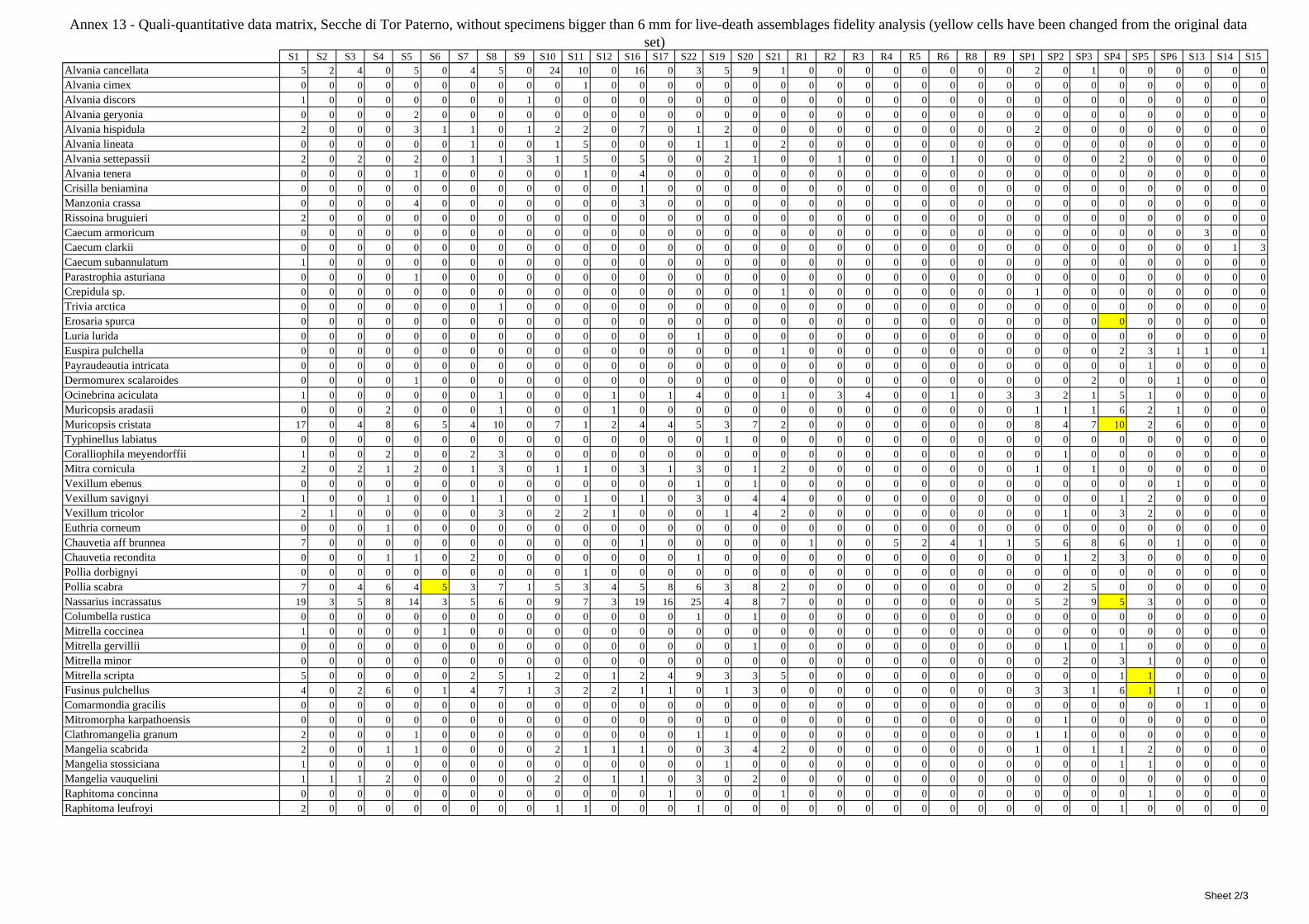
Annex 13 - Quali-quantitative data matrix, Secche di Tor Paterno, without specimens bigger than 6 mm for live-death assemblages fidelity analysis (yellow cells have been changed from the original data set)

S1 S2 S3 S4 S5 S6 S7 S8 S9 S10 S11 S12 S16 S17 S22 S19 S20 S21 R1 R2 R3 R4 R5 R6 R8 R9 SP1 SP2 SP3 SP4 SP5 SP6 S13 S14 S15Alvania cancellata 5 2 4 0 5 0 4 5 0 24 10 0 16 0 3 5 9 1 0 0 0 0 0 0 0 0 2 0 1 0 0 0 0 0 0Alvania cimex 0 0 0 0 0 0 0 0 0 0 1 0 0 0 0 0 0 0 0 0 0 0 0 0 0 0 0 0 0 0 0 0 0 0 0Alvania discors 1 0 0 0 0 0 0 0 1 0 0 0 0 0 0 0 0 0 0 0 0 0 0 0 0 0 0 0 0 0 0 0 0 0 0Alvania geryonia 0 0 0 0 2 0 0 0 0 0 0 0 0 0 0 0 0 0 0 0 0 0 0 0 0 0 0 0 0 0 0 0 0 0 0Alvania hispidula 2 0 0 0 3 1 1 0 1 2 2 0 7 0 1 2 0 0 0 0 0 0 0 0 0 0 2 0 0 0 0 0 0 0 0Alvania lineata 0 0 0 0 0 0 1 0 0 1 5 0 0 0 1 1 0 2 0 0 0 0 0 0 0 0 0 0 0 0 0 0 0 0 0Alvania settepassii 2 0 2 0 2 0 1 1 3 1 5 0 5 0 0 2 1 0 0 1 0 0 0 1 0 0 0 0 0 2 0 0 0 0 0Alvania tenera 0 0 0 0 1 0 0 0 0 0 1 0 4 0 0 0 0 0 0 0 0 0 0 0 0 0 0 0 0 0 0 0 0 0 0Crisilla beniamina 0 0 0 0 0 0 0 0 0 0 0 0 1 0 0 0 0 0 0 0 0 0 0 0 0 0 0 0 0 0 0 0 0 0 0Manzonia crassa 0 0 0 0 4 0 0 0 0 0 0 0 3 0 0 0 0 0 0 0 0 0 0 0 0 0 0 0 0 0 0 0 0 0 0Rissoina bruguieri 2 0 0 0 0 0 0 0 0 0 0 0 0 0 0 0 0 0 0 0 0 0 0 0 0 0 0 0 0 0 0 0 0 0 0Caecum armoricum 0 0 0 0 0 0 0 0 0 0 0 0 0 0 0 0 0 0 0 0 0 0 0 0 0 0 0 0 0 0 0 0 3 0 0Caecum clarkii 0 0 0 0 0 0 0 0 0 0 0 0 0 0 0 0 0 0 0 0 0 0 0 0 0 0 0 0 0 0 0 0 0 1 3Caecum subannulatum 1 0 0 0 0 0 0 0 0 0 0 0 0 0 0 0 0 0 0 0 0 0 0 0 0 0 0 0 0 0 0 0 0 0 0Parastrophia asturiana 0 0 0 0 1 0 0 0 0 0 0 0 0 0 0 0 0 0 0 0 0 0 0 0 0 0 0 0 0 0 0 0 0 0 0Crepidula sp. 0 0 0 0 0 0 0 0 0 0 0 0 0 0 0 0 0 1 0 0 0 0 0 0 0 0 1 0 0 0 0 0 0 0 0Trivia arctica 0 0 0 0 0 0 0 1 0 0 0 0 0 0 0 0 0 0 0 0 0 0 0 0 0 0 0 0 0 0 0 0 0 0 0Erosaria spurca 0 0 0 0 0 0 0 0 0 0 0 0 0 0 0 0 0 0 0 0 0 0 0 0 0 0 0 0 0 0 0 0 0 0 0Luria lurida 0 0 0 0 0 0 0 0 0 0 0 0 0 0 1 0 0 0 0 0 0 0 0 0 0 0 0 0 0 0 0 0 0 0 0Euspira pulchella 0 0 0 0 0 0 0 0 0 0 0 0 0 0 0 0 0 1 0 0 0 0 0 0 0 0 0 0 0 2 3 1 1 0 1Payraudeautia intricata 0 0 0 0 0 0 0 0 0 0 0 0 0 0 0 0 0 0 0 0 0 0 0 0 0 0 0 0 0 0 1 0 0 0 0Dermomurex scalaroides 0 0 0 0 1 0 0 0 0 0 0 0 0 0 0 0 0 0 0 0 0 0 0 0 0 0 0 0 2 0 0 1 0 0 0Ocinebrina aciculata 1 0 0 0 0 0 0 1 0 0 0 1 0 1 4 0 0 1 0 3 4 0 0 1 0 3 3 2 1 5 1 0 0 0 0Muricopsis aradasii 0 0 0 2 0 0 0 1 0 0 0 1 0 0 0 0 0 0 0 0 0 0 0 0 0 0 1 1 1 6 2 1 0 0 0Muricopsis cristata 17 0 4 8 6 5 4 10 0 7 1 2 4 4 5 3 7 2 0 0 0 0 0 0 0 0 8 4 7 10 2 6 0 0 0Typhinellus labiatus 0 0 0 0 0 0 0 0 0 0 0 0 0 0 0 1 0 0 0 0 0 0 0 0 0 0 0 0 0 0 0 0 0 0 0Coralliophila meyendorffii 1 0 0 2 0 0 2 3 0 0 0 0 0 0 0 0 0 0 0 0 0 0 0 0 0 0 0 1 0 0 0 0 0 0 0Mitra cornicula 2 0 2 1 2 0 1 3 0 1 1 0 3 1 3 0 1 2 0 0 0 0 0 0 0 0 1 0 1 0 0 0 0 0 0Vexillum ebenus 0 0 0 0 0 0 0 0 0 0 0 0 0 0 1 0 1 0 0 0 0 0 0 0 0 0 0 0 0 0 0 1 0 0 0Vexillum savignyi 1 0 0 1 0 0 1 1 0 0 1 0 1 0 3 0 4 4 0 0 0 0 0 0 0 0 0 0 0 1 2 0 0 0 0Vexillum tricolor 2 1 0 0 0 0 0 3 0 2 2 1 0 0 0 1 4 2 0 0 0 0 0 0 0 0 0 1 0 3 2 0 0 0 0Euthria corneum 0 0 0 1 0 0 0 0 0 0 0 0 0 0 0 0 0 0 0 0 0 0 0 0 0 0 0 0 0 0 0 0 0 0 0Chauvetia aff brunnea 7 0 0 0 0 0 0 0 0 0 0 0 1 0 0 0 0 0 1 0 0 5 2 4 1 1 5 6 8 6 0 1 0 0 0Chauvetia recondita 0 0 0 1 1 0 2 0 0 0 0 0 0 0 1 0 0 0 0 0 0 0 0 0 0 0 0 1 2 3 0 0 0 0 0Pollia dorbignyi 0 0 0 0 0 0 0 0 0 0 1 0 0 0 0 0 0 0 0 0 0 0 0 0 0 0 0 0 0 0 0 0 0 0 0Pollia scabra 7 0 4 6 4 5 3 7 1 5 3 4 5 8 6 3 8 2 0 0 0 0 0 0 0 0 0 2 5 0 0 0 0 0 0Nassarius incrassatus 19 3 5 8 14 3 5 6 0 9 7 3 19 16 25 4 8 7 0 0 0 0 0 0 0 0 5 2 9 5 3 0 0 0 0Columbella rustica 0 0 0 0 0 0 0 0 0 0 0 0 0 0 1 0 1 0 0 0 0 0 0 0 0 0 0 0 0 0 0 0 0 0 0Mitrella coccinea 1 0 0 0 0 1 0 0 0 0 0 0 0 0 0 0 0 0 0 0 0 0 0 0 0 0 0 0 0 0 0 0 0 0 0Mitrella gervillii 0 0 0 0 0 0 0 0 0 0 0 0 0 0 0 0 1 0 0 0 0 0 0 0 0 0 0 1 0 1 0 0 0 0 0Mitrella minor 0 0 0 0 0 0 0 0 0 0 0 0 0 0 0 0 0 0 0 0 0 0 0 0 0 0 0 2 0 3 1 0 0 0 0Mitrella scripta 5 0 0 0 0 0 2 5 1 2 0 1 2 4 9 3 3 5 0 0 0 0 0 0 0 0 0 0 0 1 1 0 0 0 0Fusinus pulchellus 4 0 2 6 0 1 4 7 1 3 2 2 1 1 0 1 3 0 0 0 0 0 0 0 0 0 3 3 1 6 1 1 0 0 0Comarmondia gracilis 0 0 0 0 0 0 0 0 0 0 0 0 0 0 0 0 0 0 0 0 0 0 0 0 0 0 0 0 0 0 0 0 1 0 0Mitromorpha karpathoensis 0 0 0 0 0 0 0 0 0 0 0 0 0 0 0 0 0 0 0 0 0 0 0 0 0 0 0 1 0 0 0 0 0 0 0Clathromangelia granum 2 0 0 0 1 0 0 0 0 0 0 0 0 0 1 1 0 0 0 0 0 0 0 0 0 0 1 1 0 0 0 0 0 0 0Mangelia scabrida 2 0 0 1 1 0 0 0 0 2 1 1 1 0 0 3 4 2 0 0 0 0 0 0 0 0 1 0 1 1 2 0 0 0 0Mangelia stossiciana 1 0 0 0 0 0 0 0 0 0 0 0 0 0 0 1 0 0 0 0 0 0 0 0 0 0 0 0 0 1 1 0 0 0 0Mangelia vauquelini 1 1 1 2 0 0 0 0 0 2 0 1 1 0 3 0 2 0 0 0 0 0 0 0 0 0 0 0 0 0 0 0 0 0 0Raphitoma concinna 0 0 0 0 0 0 0 0 0 0 0 0 0 1 0 0 0 1 0 0 0 0 0 0 0 0 0 0 0 0 1 0 0 0 0Raphitoma leufroyi 2 0 0 0 0 0 0 0 0 1 1 0 0 0 1 0 0 0 0 0 0 0 0 0 0 0 0 0 0 1 0 0 0 0 0

Sheet 2/3

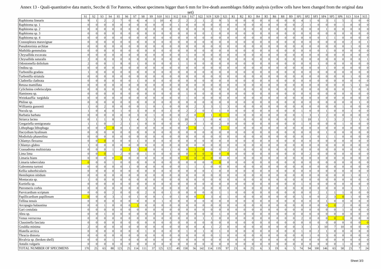
Annex 13 - Quali-quantitative data matrix, Secche di Tor Paterno, without specimens bigger than 6 mm for live-death assemblages fidelity analysis (yellow cells have been changed from the original data set)

S1 S2 S3 S4 S5 S6 S7 S8 S9 S10 S11 S12 S16 S17 S22 S19 S20 S21 R1 R2 R3 R4 R5 R6 R8 R9 SP1 SP2 SP3 SP4 SP5 SP6 S13 S14 S15Raphitoma linearis 9 1 2 2 7 0 6 4 1 10 4 2 2 2 1 2 9 5 0 0 0 0 0 0 0 0 4 1 6 3 1 5 1 0 0Raphitoma sp. 1 0 0 0 0 0 0 0 0 0 0 0 1 0 0 0 0 0 0 0 0 0 0 0 0 0 0 2 1 0 0 0 1 0 0 0Raphitoma sp. 2 0 0 0 0 0 0 0 0 0 0 0 0 0 0 0 0 1 0 0 0 0 0 0 0 0 0 0 0 0 1 0 0 0 0 0Raphitoma sp. 3 0 0 0 0 0 0 0 0 0 0 0 0 0 0 0 1 0 0 0 0 0 0 0 0 0 0 0 0 0 0 0 0 0 0 0Raphitoma sp. 4 0 0 0 0 0 0 0 0 0 0 0 0 0 0 0 0 0 0 0 0 0 0 0 0 0 0 0 0 0 1 1 0 0 0 0Crassopleura maravignae 0 0 0 0 0 0 0 0 0 0 0 0 0 0 0 0 0 0 0 0 0 0 0 0 0 0 0 0 0 0 0 0 2 0 1Pseudotorinia architae 0 0 0 0 0 0 0 0 0 0 0 0 0 0 0 0 0 0 0 0 0 0 0 0 0 0 0 0 0 0 0 0 1 0 0Mathilda gemmulata 0 0 0 0 0 0 0 0 0 0 0 0 0 0 0 0 0 0 0 0 0 0 0 0 0 0 0 0 0 1 0 0 0 0 0Chrysallida excavata 0 0 0 0 0 0 0 0 0 0 0 0 1 0 0 0 0 0 0 0 0 0 0 0 0 0 0 0 0 0 0 0 0 0 0Chrysallida suturalis 2 0 0 0 0 0 0 0 0 0 0 0 0 0 0 0 0 0 0 0 0 0 0 0 0 0 0 0 0 0 0 0 0 0 1Odostomella doliolum 2 0 0 1 8 0 1 0 0 0 0 1 1 0 0 0 0 0 0 0 0 0 0 0 0 0 0 0 1 0 0 0 0 0 0Ondina sp. 0 0 0 0 0 0 0 0 0 0 0 0 0 0 0 0 0 0 0 0 0 0 0 0 0 0 0 0 0 1 0 0 0 0 0Turbonilla gradata 1 0 0 0 0 0 0 0 0 0 0 0 0 0 0 0 0 0 0 0 0 0 0 0 0 0 0 0 0 0 0 0 0 0 0Turbonilla striatula 0 0 0 0 0 0 0 0 0 0 0 0 0 0 0 0 0 0 0 0 0 0 0 0 0 0 0 0 0 0 0 0 1 0 0Clathrella clathrata 0 0 0 0 0 0 1 0 0 0 0 0 0 0 0 0 0 0 0 0 0 0 0 0 0 0 0 0 0 0 0 0 0 0 0Retusa mamillata 0 0 0 0 0 0 0 0 0 0 0 0 0 0 0 0 0 0 0 0 0 0 0 0 0 0 0 0 0 0 0 0 5 1 14Cylichnina crebrisculpta 0 0 0 0 0 0 0 0 0 0 0 0 0 0 0 0 0 0 0 0 0 0 0 0 0 0 0 0 0 0 0 0 1 0 0Haminoea sp. 0 0 0 0 0 0 0 0 0 0 0 0 1 0 0 0 0 0 0 0 0 0 0 0 0 0 0 0 0 0 0 0 0 0 0Weinkauffia turgidula 0 0 0 0 0 0 0 0 0 0 0 0 1 0 0 0 0 0 0 0 0 0 0 0 0 0 0 0 0 0 0 0 0 0 0Philine sp. 0 0 0 0 0 0 0 0 0 0 0 0 0 0 0 0 0 0 0 0 0 0 0 0 0 0 0 0 0 0 0 0 0 1 0Williamia gussonii 1 0 2 0 0 0 0 1 0 1 0 0 0 2 3 3 1 3 0 0 0 0 0 0 0 0 0 0 0 0 0 1 0 0 0Nucula sp. 1 0 4 0 1 0 3 0 0 0 3 0 2 2 0 1 1 0 0 0 0 0 0 0 0 0 1 0 0 1 0 0 1 0 0Barbatia barbata 0 0 0 0 0 0 3 0 1 0 0 0 2 0 2 1 0 1 0 0 0 0 0 0 0 0 1 3 1 2 0 0 0 0 0Striarca lactea 0 1 1 8 3 1 4 3 3 0 0 1 18 3 1 0 4 1 0 0 0 0 0 0 0 0 1 18 1 1 3 2 2 1 0Gregariella semigranata 1 1 0 1 2 1 1 0 0 0 0 0 2 0 1 0 2 0 0 0 0 0 0 0 0 0 1 0 0 0 0 1 0 0 0Lithophaga lithophaga 0 0 0 0 0 1 0 0 0 0 0 0 0 0 1 0 0 1 0 0 0 0 0 0 0 0 0 0 0 0 0 0 0 0 0Dacrydium hyalinum 0 0 0 0 0 0 0 0 0 0 0 0 0 0 0 0 0 0 0 0 0 0 0 0 0 0 0 0 0 1 0 0 0 0 0Modiolula phaseolina 0 0 0 0 0 0 0 0 0 0 0 0 0 0 0 0 0 0 0 0 0 0 0 0 0 0 0 1 0 1 1 0 0 0 0Chlamys flexuosa 0 0 0 0 0 0 1 0 0 0 0 0 0 0 0 0 0 0 0 0 0 0 0 0 0 0 0 0 0 0 0 0 0 0 0Chlamys glabra 1 0 0 0 0 0 0 0 0 0 0 0 0 0 0 0 0 0 0 0 0 0 0 0 0 0 0 0 0 0 0 0 0 0 0Crassadoma multistriata 0 0 0 1 0 1 3 0 0 0 1 0 0 1 0 0 0 2 0 0 0 0 0 0 0 0 0 0 0 0 0 0 0 0 0Lima lima 0 0 0 1 2 0 0 1 0 0 0 0 0 0 0 0 0 0 0 0 0 0 0 0 0 0 0 2 0 0 0 0 0 0 0Limaria hians 0 0 0 0 0 0 0 0 0 0 0 0 0 0 0 0 0 0 0 0 0 0 0 0 0 0 0 0 0 0 0 0 0 0 0Limaria tuberculata 0 0 0 1 0 0 0 0 0 0 0 0 0 0 0 0 0 0 0 0 0 0 0 0 0 0 0 0 0 0 0 0 0 0 0Galeomma turtoni 0 0 0 0 0 1 0 4 0 0 0 0 1 1 1 0 0 0 0 0 0 0 0 0 0 0 0 0 0 0 0 0 0 0 0Kellia suborbicularis 0 0 0 0 0 0 0 0 0 0 0 0 0 0 0 1 0 0 0 0 0 0 0 0 0 0 0 0 0 0 0 0 0 0 0Hemilepton nitidum 0 0 0 0 0 0 0 0 0 0 0 0 0 0 0 0 0 0 0 0 0 0 0 0 0 0 0 0 0 0 0 0 1 0 1Montacuta sp. 1 0 0 0 0 0 0 0 0 0 0 0 0 0 0 0 0 0 0 0 0 0 0 0 0 0 0 0 0 0 0 0 0 0 0Kurtiella sp. 0 0 0 0 0 0 0 0 0 0 0 0 0 0 0 0 0 0 0 0 0 0 0 0 0 0 1 0 0 0 0 0 0 0 0Pteromeris corbis 0 0 0 0 0 0 0 0 0 0 0 0 0 0 0 0 0 0 0 0 0 0 0 0 0 0 0 0 0 0 0 0 1 3 1Parvicardium scriptum 0 0 0 2 0 0 0 2 0 0 1 0 0 0 0 0 1 1 0 0 0 0 0 0 0 0 0 0 2 1 1 1 0 0 0Papillicardium papillosum 0 0 0 3 1 0 1 0 0 1 0 1 0 0 1 3 4 1 0 0 0 0 0 0 0 0 5 0 0 2 3 8 1 0 0Tellina tenuis 0 0 0 0 0 0 0 0 0 1 0 0 0 0 0 0 0 0 0 0 0 0 0 0 0 0 0 0 0 1 0 0 0 0 0Arcopagia balaustina 0 0 1 0 0 0 1 0 0 0 0 0 0 0 0 0 0 0 0 0 0 0 0 0 0 0 0 0 0 0 0 2 0 0 0Gari costulata 0 0 0 0 0 0 0 0 0 0 0 0 0 0 0 0 0 0 0 0 0 0 0 0 0 0 0 0 0 0 0 1 0 0 0Abra sp. 0 0 1 0 0 0 0 0 0 0 0 0 0 0 0 0 1 0 0 0 0 0 0 0 0 0 0 0 0 0 0 0 0 0 0Venus verrucosa 0 0 0 0 0 0 0 0 0 0 0 0 0 0 1 1 0 0 0 0 0 0 0 0 0 0 2 0 0 0 0 1 0 0 0Clausinella fasciata 0 0 0 0 0 0 0 0 0 0 0 0 0 0 0 0 0 0 0 0 0 0 0 0 0 0 0 0 0 0 0 0 0 0 0Gouldia minima 2 0 0 0 0 0 0 0 0 0 0 0 0 0 4 1 2 0 0 0 0 0 0 0 0 0 3 1 3 10 7 10 0 0 0Hiatella arctica 0 0 0 0 0 0 0 1 0 0 0 0 1 0 1 0 1 0 0 0 0 0 0 0 0 0 1 0 2 1 0 0 0 0 0Thracia distorta 0 0 0 0 0 0 0 0 0 0 0 0 0 0 0 0 1 0 0 0 0 0 0 0 0 0 0 1 0 3 0 0 0 0 0Bivalvia sp. (broken shell) 0 0 0 1 0 0 0 0 0 0 0 0 0 0 0 0 0 0 0 0 0 0 0 0 0 0 0 0 0 0 0 0 0 0 0Antalis vulgaris 0 0 0 0 0 0 0 0 0 0 0 0 0 0 0 0 0 0 0 0 0 0 0 0 0 0 0 0 0 0 0 1 0 0 0TOTAL NUMBER OF SPECIMENS 170 25 63 88 123 25 114 111 37 125 122 49 158 56 142 114 119 97 23 6 25 6 3 19 6 5 74 94 100 146 63 58 23 7 24

Sheet 3/3

ANNEX 14

QUALI-QUANTITATIVE DATA OF THE POSIDONIA OCEANICA DEATH ASSEMBLAGE

IN SECCHE DI TOR PATERNO

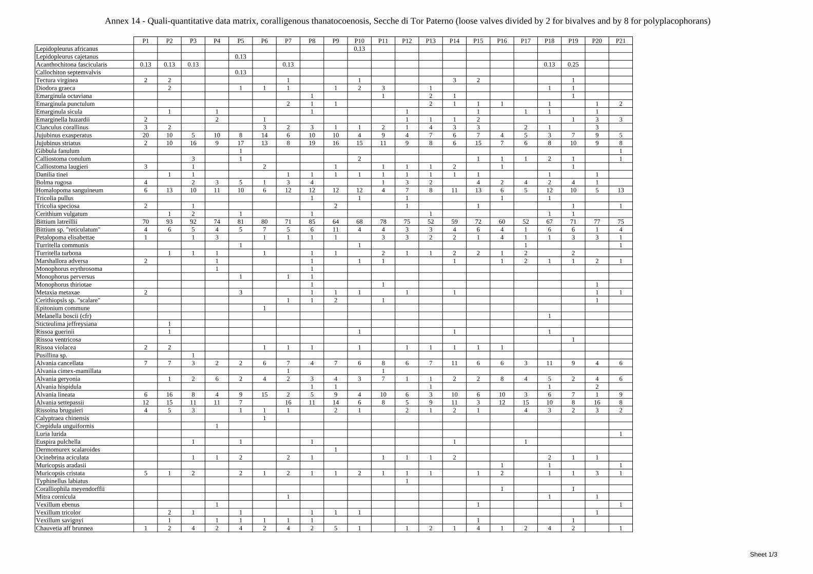
Annex 14 - Quali-quantitative data matrix, coralligenous thanatocoenosis, Secche di Tor Paterno (loose valves divided by 2 for bivalves and by 8 for polyplacophorans)

P1 P2 P3 P4 P5 P6 P7 P8 P9 P10 P11 P12 P13 P14 P15 P16 P17 P18 P19 P20 P21Lepidopleurus africanus 0.13Lepidopleurus cajetanus 0.13Acanthochitona fascicularis 0.13 0.13 0.13 0.13 0.13 0.25Callochiton septemvalvis 0.13Tectura virginea 2 2 1 1 3 2 1Diodora graeca 2 1 1 1 1 2 3 1 1 1Emarginula octaviana 1 1 2 1 1Emarginula punctulum 2 1 1 2 1 1 1 1 1 2Emarginula sicula 1 1 1 1 1 1 1 1Emarginella huzardii 2 2 1 1 1 1 2 1 3 3Clanculus corallinus 3 2 3 2 3 1 1 2 1 4 3 3 2 1 3Jujubinus exasperatus 20 10 5 10 8 14 6 10 10 4 9 4 7 6 7 4 5 3 7 9 5Jujubinus striatus 2 10 16 9 17 13 8 19 16 15 11 9 8 6 15 7 6 8 10 9 8Gibbula fanulum 1 1Calliostoma conulum 3 1 2 1 1 1 2 1 1Calliostoma laugieri 3 1 2 1 1 1 1 2 1 1Danilia tinei 1 1 1 1 1 1 1 1 1 1 1 1 1Bolma rugosa 4 2 3 5 1 3 4 1 3 2 4 2 4 2 4 1Homalopoma sanguineum 6 13 10 11 10 6 12 12 12 12 4 7 8 11 13 6 5 12 10 5 13Tricolia pullus 1 1 1 1 1Tricolia speciosa 2 1 2 1 1 1 1Cerithium vulgatum 1 2 1 1 1 1 1Bittium latreillii 70 93 92 74 81 80 71 85 64 68 78 75 52 59 72 60 52 67 71 77 75Bittium sp. "reticulatum" 4 6 5 4 5 7 5 6 11 4 4 3 3 4 6 4 1 6 6 1 4Petalopoma elisabettae 1 1 3 1 1 1 1 3 3 2 2 1 4 1 1 3 3 1Turritella communis 1 1 1 1Turritella turbona 1 1 1 1 1 1 2 1 1 2 2 1 2 2Marshallora adversa 2 1 1 1 1 1 1 2 1 1 2 1Monophorus erythrosoma 1 1Monophorus perversus 1 1 1Monophorus thiriotae 1 1 1Metaxia metaxae 2 3 1 1 1 1 1 1 1Cerithiopsis sp. "scalare" 1 1 2 1 1Epitonium commune 1Melanella boscii (cfr) 1Sticteulima jeffreysiana 1Rissoa guerinii 1 1 1 1Rissoa ventricosa 1Rissoa violacea 2 2 1 1 1 1 1 1 1 1 1Pusillina sp. 1Alvania cancellata 7 7 3 2 2 6 7 4 7 6 8 6 7 11 6 6 3 11 9 4 6Alvania cimex-mamillata 1 1Alvania geryonia 1 2 6 2 4 2 3 4 3 7 1 1 2 2 8 4 5 2 4 6Alvania hispidula 1 1 1 1 2Alvania lineata 6 16 8 4 9 15 2 5 9 4 10 6 3 10 6 10 3 6 7 1 9Alvania settepassii 12 15 11 11 7 16 11 14 6 8 5 9 11 3 12 15 10 8 16 8Rissoina bruguieri 4 5 3 1 1 1 2 1 2 1 2 1 4 3 2 3 2Calyptraea chinensis 1Crepidula unguiformis 1Luria lurida 1Euspira pulchella 1 1 1 1 1Dermomurex scalaroides 1Ocinebrina aciculata 1 1 2 2 1 1 1 1 2 2 1 1Muricopsis aradasii 1 1 1Muricopsis cristata 5 1 2 2 1 2 1 1 2 1 1 1 1 2 1 1 3 1Typhinellus labiatus 1Coralliophila meyendorffii 1 1Mitra cornicula 1 1 1Vexillum ebenus 1 1 1Vexillum tricolor 2 1 1 1 1 1 1Vexillum savignyi 1 1 1 1 1 1 1 1Chauvetia aff brunnea 1 2 4 2 4 2 4 2 5 1 1 2 1 4 1 2 4 2 1

Sheet 1/3

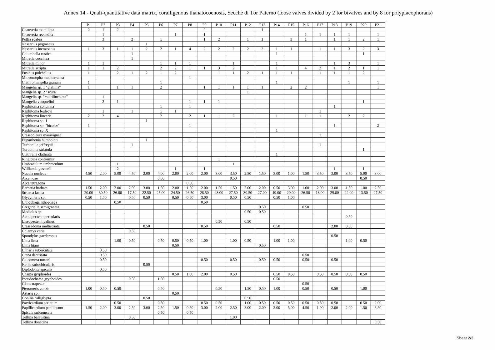
Annex 14 - Quali-quantitative data matrix, coralligenous thanatocoenosis, Secche di Tor Paterno (loose valves divided by 2 for bivalves and by 8 for polyplacophorans)

P1 P2 P3 P4 P5 P6 P7 P8 P9 P10 P11 P12 P13 P14 P15 P16 P17 P18 P19 P20 P21Chauvetia mamillata 2 1 2 2 1Chauvetia recondita 1 1 1 1 1 1 1 1Pollia scabra 3 2 1 1 2 1 1 3 1 1 1 2 1Nassarius pygmaeus 1Nassarius incrassatus 1 3 1 1 2 2 1 4 2 2 2 2 2 1 1 1 1 3 2 3Columbella rustica 1 1 1Mitrella coccinea 1Mitrella minor 1 1 1 1 1 1 1 1 3 1Mitrella scripta 1 1 2 2 2 1 1 3 2 1 4 2 1 2 1 1Fusinus pulchellus 1 2 1 2 1 2 1 1 2 1 1 1 1 1 1 2Mitromorpha mediterranea 1Clathromangelia granum 1 1 1 1 1Mangelia sp. 1 "giallina" 1 1 1 2 1 1 1 1 1 2 2 1Mangelia sp. 2 "scura" 1Mangelia sp. "multilineolata" 1Mangelia vauquelini 2 1 1 1 1 1Raphitoma concinna 1 1 1Raphitoma leufroyi 1 1 1 1 1Raphitoma linearis 2 2 4 2 2 1 1 2 1 1 1 2 2Raphitoma sp. 1 1Raphitoma sp. "bicolor" 1 1 1 2Raphitoma sp. X 1Crassopleura maravignae 1Euparthenia humboldti 1 1Turbonilla jeffreysii 1 1Turbonilla striatula 1Clathrella clathrata 1Ringicula conformis 1Umbraculum umbraculum 1 1Williamia gussonii 2 1 1 1 1Nucula nucleus 4.50 2.00 5.00 4.50 2.00 4.00 2.00 2.00 2.00 3.00 3.50 2.50 1.50 3.00 1.00 1.50 3.50 3.00 3.50 5.00 3.00Arca noae 0.50 0.50 0.50Arca tetragona 0.50Barbatia barbata 1.50 2.00 2.00 2.00 3.00 1.50 2.00 1.50 2.00 1.50 1.50 3.00 2.00 0.50 3.00 1.00 2.00 3.00 1.50 1.00 2.50Striarca lactea 20.00 30.50 26.00 17.50 22.50 25.00 24.50 26.50 28.50 48.00 27.50 30.50 27.00 49.00 20.00 26.50 18.00 29.00 22.00 13.50 27.50Glycymeris sp. 0.50 1.50 0.50 0.50 0.50 0.50 3.00 0.50 0.50 0.50 1.00Lithophaga lithophaga 0.50 0.50Gregariella semigranata 0.50 0.50Modiolus sp. 0.50 0.50Aequipecten opercularis 0.50Lissopecten hyalinus 0.50 0.50Crassadoma multistriata 0.50 0.50 0.50 2.00 0.50Chlamys varia 0.50Spondylus gaederopus 0.50Lima lima 1.00 0.50 0.50 0.50 0.50 1.00 1.00 0.50 1.00 1.00 1.00 0.50Lima hians 0.50 0.50Limaria tuberculata 0.50Ctena decussata 0.50 0.50Galeomma turtoni 0.50 0.50 0.50 0.50 0.50 0.50 0.50Kellia suborbicularis 0.50Diplodonta apicalis 0.50Chama gryphoides 0.50 1.00 2.00 0.50 0.50 0.50 0.50 0.50 0.50 0.50Pseudochama gryphoides 0.50 1.50 0.50Glans trapezia 0.50Pteromeris corbis 1.00 0.50 0.50 0.50 0.50 1.50 0.50 1.00 0.50 0.50 1.00Astarte sp. 0.50Gonilia calliglypta 0.50 0.50Parvicardium scriptum 0.50 0.50 0.50 0.50 1.00 0.50 0.50 0.50 0.50 0.50 0.50 0.50 2.00Papillicardium papillosum 1.50 2.00 3.00 2.50 3.00 2.50 1.50 0.50 3.00 2.00 2.50 3.00 2.00 2.00 5.00 4.50 1.00 2.00 2.00 1.50 3.50Spisula subtruncata 0.50 0.50Tellina balaustina 0.50 1.00Tellina donacina 0.50

Sheet 2/3

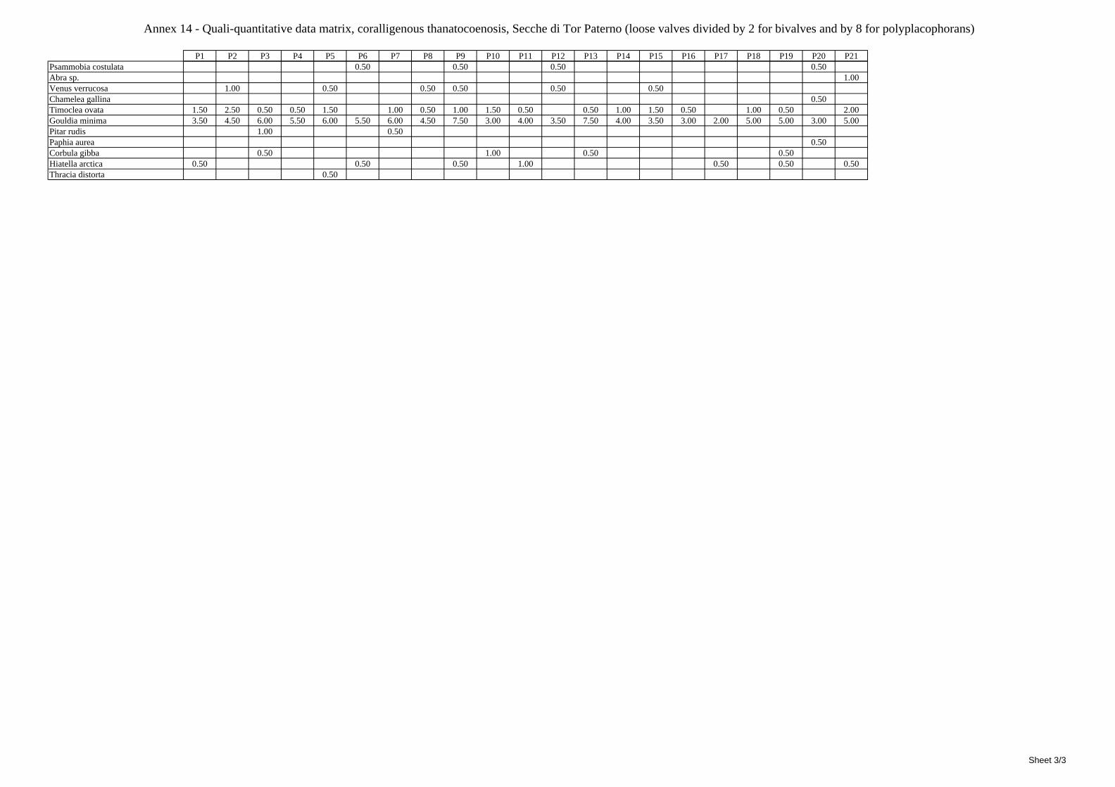
Annex 14 - Quali-quantitative data matrix, coralligenous thanatocoenosis, Secche di Tor Paterno (loose valves divided by 2 for bivalves and by 8 for polyplacophorans)

P1 P2 P3 P4 P5 P6 P7 P8 P9 P10 P11 P12 P13 P14 P15 P16 P17 P18 P19 P20 P21Psammobia costulata 0.50 0.50 0.50 0.50Abra sp. 1.00Venus verrucosa 1.00 0.50 0.50 0.50 0.50 0.50Chamelea gallina 0.50Timoclea ovata 1.50 2.50 0.50 0.50 1.50 1.00 0.50 1.00 1.50 0.50 0.50 1.00 1.50 0.50 1.00 0.50 2.00Gouldia minima 3.50 4.50 6.00 5.50 6.00 5.50 6.00 4.50 7.50 3.00 4.00 3.50 7.50 4.00 3.50 3.00 2.00 5.00 5.00 3.00 5.00Pitar rudis 1.00 0.50Paphia aurea 0.50Corbula gibba 0.50 1.00 0.50 0.50Hiatella arctica 0.50 0.50 0.50 1.00 0.50 0.50 0.50Thracia distorta 0.50

Sheet 3/3

ANNEX 15

QUALI-QUANTITATIVE DATA OF THE CORALLIGENOUS DEATH ASSEMBLAGE

IN SECCHE DI TOR PATERNO

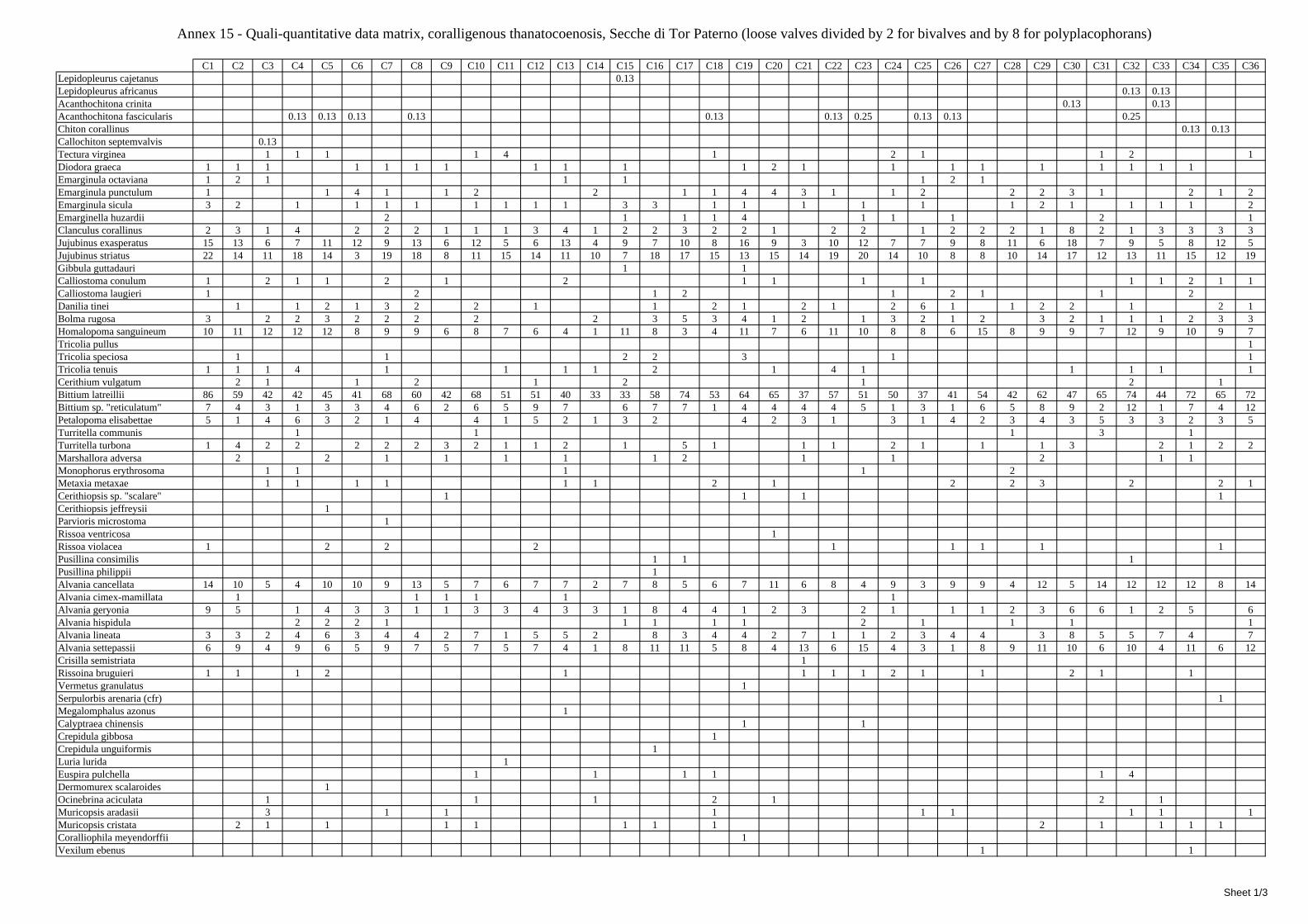
Annex 15 - Quali-quantitative data matrix, coralligenous thanatocoenosis, Secche di Tor Paterno (loose valves divided by 2 for bivalves and by 8 for polyplacophorans)

C1 C2 C3 C4 C5 C6 C7 C8 C9 C10 C11 C12 C13 C14 C15 C16 C17 C18 C19 C20 C21 C22 C23 C24 C25 C26 C27 C28 C29 C30 C31 C32 C33 C34 C35 C36Lepidopleurus cajetanus 0.13Lepidopleurus africanus 0.13 0.13Acanthochitona crinita 0.13 0.13Acanthochitona fascicularis 0.13 0.13 0.13 0.13 0.13 0.13 0.25 0.13 0.13 0.25Chiton corallinus 0.13 0.13Callochiton septemvalvis 0.13Tectura virginea 1 1 1 1 4 1 2 1 1 2 1Diodora graeca 1 1 1 1 1 1 1 1 1 1 1 2 1 1 1 1 1 1 1 1 1Emarginula octaviana 1 2 1 1 1 1 2 1Emarginula punctulum 1 1 4 1 1 2 2 1 1 4 4 3 1 1 2 2 2 3 1 2 1 2Emarginula sicula 3 2 1 1 1 1 1 1 1 1 3 3 1 1 1 1 1 1 2 1 1 1 1 2Emarginella huzardii 2 1 1 1 4 1 1 1 2 1Clanculus corallinus 2 3 1 4 2 2 2 1 1 1 3 4 1 2 2 3 2 2 1 2 2 1 2 2 2 1 8 2 1 3 3 3 3Jujubinus exasperatus 15 13 6 7 11 12 9 13 6 12 5 6 13 4 9 7 10 8 16 9 3 10 12 7 7 9 8 11 6 18 7 9 5 8 12 5Jujubinus striatus 22 14 11 18 14 3 19 18 8 11 15 14 11 10 7 18 17 15 13 15 14 19 20 14 10 8 8 10 14 17 12 13 11 15 12 19Gibbula guttadauri 1 1Calliostoma conulum 1 2 1 1 2 1 2 1 1 1 1 1 1 2 1 1Calliostoma laugieri 1 2 1 2 1 2 1 1 2Danilia tinei 1 1 2 1 3 2 2 1 1 2 1 2 1 2 6 1 1 2 2 1 2 1Bolma rugosa 3 2 2 3 2 2 2 2 2 3 5 3 4 1 2 1 3 2 1 2 3 2 1 1 1 2 3 3Homalopoma sanguineum 10 11 12 12 12 8 9 9 6 8 7 6 4 1 11 8 3 4 11 7 6 11 10 8 8 6 15 8 9 9 7 12 9 10 9 7Tricolia pullus 1Tricolia speciosa 1 1 2 2 3 1 1Tricolia tenuis 1 1 1 4 1 1 1 1 2 1 4 1 1 1 1 1Cerithium vulgatum 2 1 1 2 1 2 1 2 1Bittium latreillii 86 59 42 42 45 41 68 60 42 68 51 51 40 33 33 58 74 53 64 65 37 57 51 50 37 41 54 42 62 47 65 74 44 72 65 72Bittium sp. "reticulatum" 7 4 3 1 3 3 4 6 2 6 5 9 7 6 7 7 1 4 4 4 4 5 1 3 1 6 5 8 9 2 12 1 7 4 12Petalopoma elisabettae 5 1 4 6 3 2 1 4 4 1 5 2 1 3 2 4 2 3 1 3 1 4 2 3 4 3 5 3 3 2 3 5Turritella communis 1 1 1 3 1Turritella turbona 1 4 2 2 2 2 2 3 2 1 1 2 1 5 1 1 1 2 1 1 1 3 2 1 2 2Marshallora adversa 2 2 1 1 1 1 1 2 1 1 2 1 1Monophorus erythrosoma 1 1 1 1 2Metaxia metaxae 1 1 1 1 1 1 2 1 2 2 3 2 2 1Cerithiopsis sp. "scalare" 1 1 1 1Cerithiopsis jeffreysii 1Parvioris microstoma 1Rissoa ventricosa 1Rissoa violacea 1 2 2 2 1 1 1 1 1Pusillina consimilis 1 1 1Pusillina philippii 1Alvania cancellata 14 10 5 4 10 10 9 13 5 7 6 7 7 2 7 8 5 6 7 11 6 8 4 9 3 9 9 4 12 5 14 12 12 12 8 14Alvania cimex-mamillata 1 1 1 1 1 1Alvania geryonia 9 5 1 4 3 3 1 1 3 3 4 3 3 1 8 4 4 1 2 3 2 1 1 1 2 3 6 6 1 2 5 6Alvania hispidula 2 2 2 1 1 1 1 1 2 1 1 1 1Alvania lineata 3 3 2 4 6 3 4 4 2 7 1 5 5 2 8 3 4 4 2 7 1 1 2 3 4 4 3 8 5 5 7 4 7Alvania settepassii 6 9 4 9 6 5 9 7 5 7 5 7 4 1 8 11 11 5 8 4 13 6 15 4 3 1 8 9 11 10 6 10 4 11 6 12Crisilla semistriata 1Rissoina bruguieri 1 1 1 2 1 1 1 1 2 1 1 2 1 1Vermetus granulatus 1Serpulorbis arenaria (cfr) 1Megalomphalus azonus 1Calyptraea chinensis 1 1Crepidula gibbosa 1Crepidula unguiformis 1Luria lurida 1Euspira pulchella 1 1 1 1 1 4Dermomurex scalaroides 1Ocinebrina aciculata 1 1 1 2 1 2 1Muricopsis aradasii 3 1 1 1 1 1 1 1 1Muricopsis cristata 2 1 1 1 1 1 1 1 2 1 1 1 1Coralliophila meyendorffii 1Vexilum ebenus 1 1

Sheet 1/3

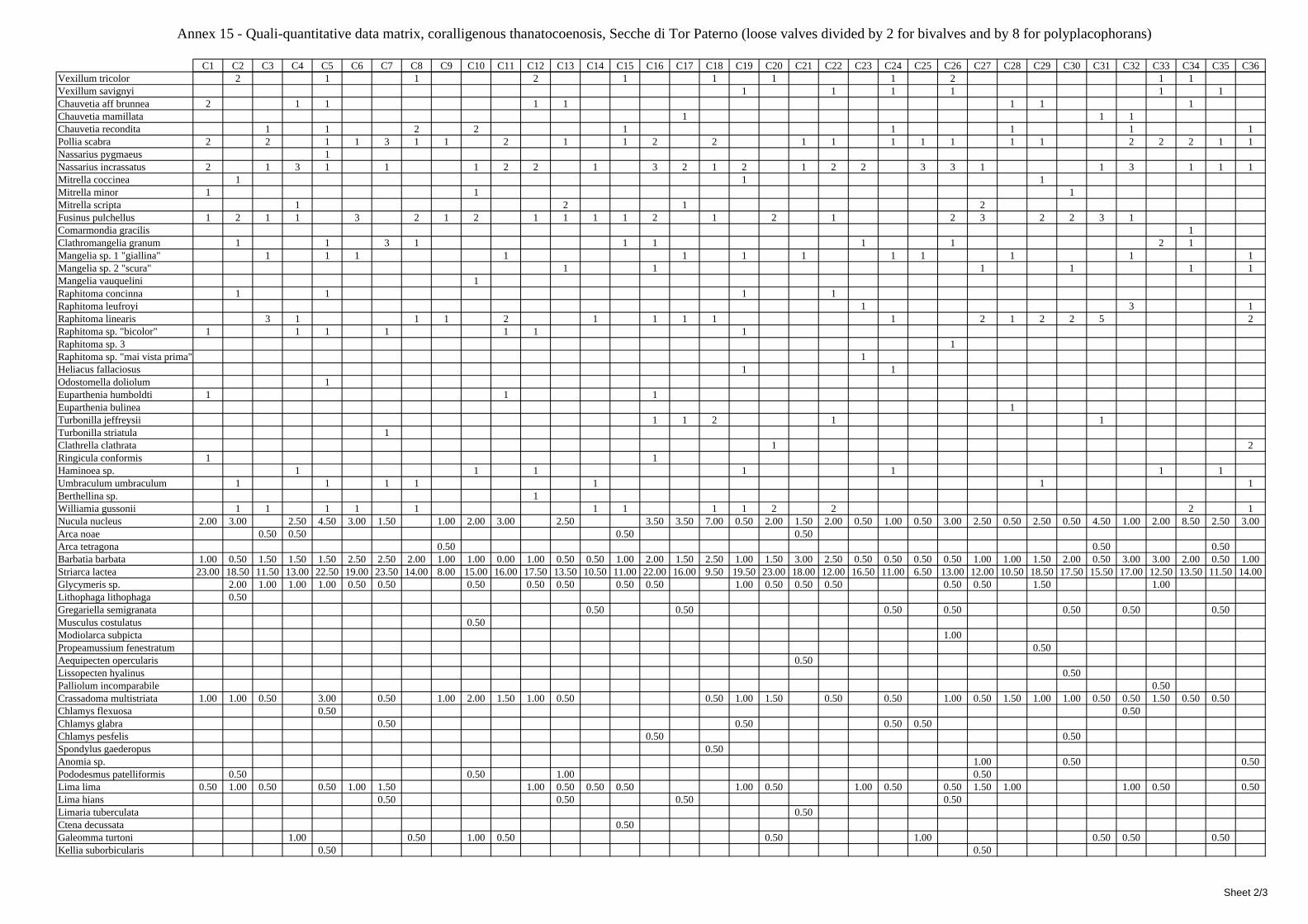
Annex 15 - Quali-quantitative data matrix, coralligenous thanatocoenosis, Secche di Tor Paterno (loose valves divided by 2 for bivalves and by 8 for polyplacophorans)

C1 C2 C3 C4 C5 C6 C7 C8 C9 C10 C11 C12 C13 C14 C15 C16 C17 C18 C19 C20 C21 C22 C23 C24 C25 C26 C27 C28 C29 C30 C31 C32 C33 C34 C35 C36Vexillum tricolor 2 1 1 2 1 1 1 1 2 1 1Vexillum savignyi 1 1 1 1 1 1Chauvetia aff brunnea 2 1 1 1 1 1 1 1Chauvetia mamillata 1 1 1Chauvetia recondita 1 1 2 2 1 1 1 1 1Pollia scabra 2 2 1 1 3 1 1 2 1 1 2 2 1 1 1 1 1 1 1 2 2 2 1 1Nassarius pygmaeus 1Nassarius incrassatus 2 1 3 1 1 1 2 2 1 3 2 1 2 1 2 2 3 3 1 1 3 1 1 1Mitrella coccinea 1 1 1Mitrella minor 1 1 1Mitrella scripta 1 2 1 2Fusinus pulchellus 1 2 1 1 3 2 1 2 1 1 1 1 2 1 2 1 2 3 2 2 3 1Comarmondia gracilis 1Clathromangelia granum 1 1 3 1 1 1 1 1 2 1Mangelia sp. 1 "giallina" 1 1 1 1 1 1 1 1 1 1 1 1Mangelia sp. 2 "scura" 1 1 1 1 1 1Mangelia vauquelini 1Raphitoma concinna 1 1 1 1Raphitoma leufroyi 1 3 1Raphitoma linearis 3 1 1 1 2 1 1 1 1 1 2 1 2 2 5 2Raphitoma sp. "bicolor" 1 1 1 1 1 1 1Raphitoma sp. 3 1Raphitoma sp. "mai vista prima" 1Heliacus fallaciosus 1 1Odostomella doliolum 1Euparthenia humboldti 1 1 1Euparthenia bulinea 1Turbonilla jeffreysii 1 1 2 1 1Turbonilla striatula 1Clathrella clathrata 1 2Ringicula conformis 1 1Haminoea sp. 1 1 1 1 1 1 1Umbraculum umbraculum 1 1 1 1 1 1 1Berthellina sp. 1Williamia gussonii 1 1 1 1 1 1 1 1 1 2 2 2 1Nucula nucleus 2.00 3.00 2.50 4.50 3.00 1.50 1.00 2.00 3.00 2.50 3.50 3.50 7.00 0.50 2.00 1.50 2.00 0.50 1.00 0.50 3.00 2.50 0.50 2.50 0.50 4.50 1.00 2.00 8.50 2.50 3.00Arca noae 0.50 0.50 0.50 0.50Arca tetragona 0.50 0.50 0.50Barbatia barbata 1.00 0.50 1.50 1.50 1.50 2.50 2.50 2.00 1.00 1.00 0.00 1.00 0.50 0.50 1.00 2.00 1.50 2.50 1.00 1.50 3.00 2.50 0.50 0.50 0.50 0.50 1.00 1.00 1.50 2.00 0.50 3.00 3.00 2.00 0.50 1.00Striarca lactea 23.00 18.50 11.50 13.00 22.50 19.00 23.50 14.00 8.00 15.00 16.00 17.50 13.50 10.50 11.00 22.00 16.00 9.50 19.50 23.00 18.00 12.00 16.50 11.00 6.50 13.00 12.00 10.50 18.50 17.50 15.50 17.00 12.50 13.50 11.50 14.00Glycymeris sp. 2.00 1.00 1.00 1.00 0.50 0.50 0.50 0.50 0.50 0.50 0.50 1.00 0.50 0.50 0.50 0.50 0.50 1.50 1.00Lithophaga lithophaga 0.50Gregariella semigranata 0.50 0.50 0.50 0.50 0.50 0.50 0.50Musculus costulatus 0.50Modiolarca subpicta 1.00Propeamussium fenestratum 0.50Aequipecten opercularis 0.50Lissopecten hyalinus 0.50Palliolum incomparabile 0.50Crassadoma multistriata 1.00 1.00 0.50 3.00 0.50 1.00 2.00 1.50 1.00 0.50 0.50 1.00 1.50 0.50 0.50 1.00 0.50 1.50 1.00 1.00 0.50 0.50 1.50 0.50 0.50Chlamys flexuosa 0.50 0.50Chlamys glabra 0.50 0.50 0.50 0.50Chlamys pesfelis 0.50 0.50Spondylus gaederopus 0.50Anomia sp. 1.00 0.50 0.50Pododesmus patelliformis 0.50 0.50 1.00 0.50Lima lima 0.50 1.00 0.50 0.50 1.00 1.50 1.00 0.50 0.50 0.50 1.00 0.50 1.00 0.50 0.50 1.50 1.00 1.00 0.50 0.50Lima hians 0.50 0.50 0.50 0.50Limaria tuberculata 0.50Ctena decussata 0.50Galeomma turtoni 1.00 0.50 1.00 0.50 0.50 1.00 0.50 0.50 0.50Kellia suborbicularis 0.50 0.50

Sheet 2/3

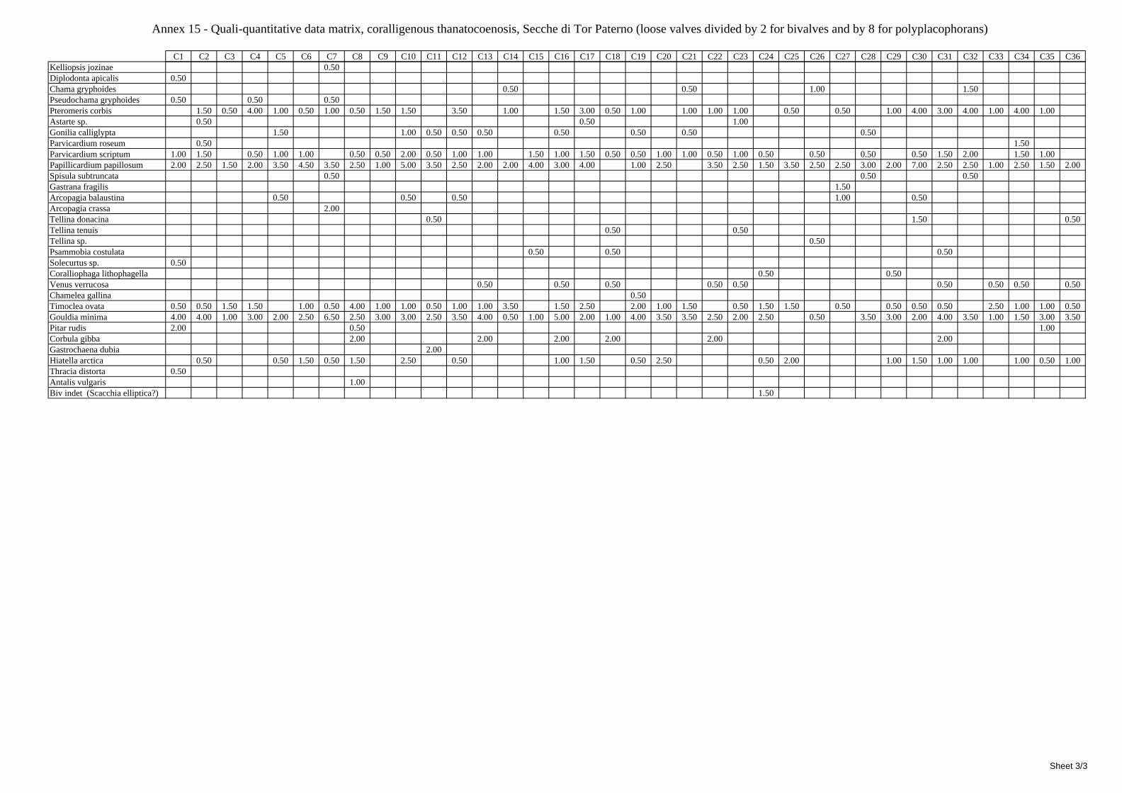
Annex 15 - Quali-quantitative data matrix, coralligenous thanatocoenosis, Secche di Tor Paterno (loose valves divided by 2 for bivalves and by 8 for polyplacophorans)

C1 C2 C3 C4 C5 C6 C7 C8 C9 C10 C11 C12 C13 C14 C15 C16 C17 C18 C19 C20 C21 C22 C23 C24 C25 C26 C27 C28 C29 C30 C31 C32 C33 C34 C35 C36Kelliopsis jozinae 0.50Diplodonta apicalis 0.50Chama gryphoides 0.50 0.50 1.00 1.50Pseudochama gryphoides 0.50 0.50 0.50Pteromeris corbis 1.50 0.50 4.00 1.00 0.50 1.00 0.50 1.50 1.50 3.50 1.00 1.50 3.00 0.50 1.00 1.00 1.00 1.00 0.50 0.50 1.00 4.00 3.00 4.00 1.00 4.00 1.00Astarte sp. 0.50 0.50 1.00Gonilia calliglypta 1.50 1.00 0.50 0.50 0.50 0.50 0.50 0.50 0.50Parvicardium roseum 0.50 1.50Parvicardium scriptum 1.00 1.50 0.50 1.00 1.00 0.50 0.50 2.00 0.50 1.00 1.00 1.50 1.00 1.50 0.50 0.50 1.00 1.00 0.50 1.00 0.50 0.50 0.50 0.50 1.50 2.00 1.50 1.00Papillicardium papillosum 2.00 2.50 1.50 2.00 3.50 4.50 3.50 2.50 1.00 5.00 3.50 2.50 2.00 2.00 4.00 3.00 4.00 1.00 2.50 3.50 2.50 1.50 3.50 2.50 2.50 3.00 2.00 7.00 2.50 2.50 1.00 2.50 1.50 2.00Spisula subtruncata 0.50 0.50 0.50Gastrana fragilis 1.50Arcopagia balaustina 0.50 0.50 0.50 1.00 0.50Arcopagia crassa 2.00Tellina donacina 0.50 1.50 0.50Tellina tenuis 0.50 0.50Tellina sp. 0.50Psammobia costulata 0.50 0.50 0.50Solecurtus sp. 0.50Coralliophaga lithophagella 0.50 0.50Venus verrucosa 0.50 0.50 0.50 0.50 0.50 0.50 0.50 0.50 0.50Chamelea gallina 0.50Timoclea ovata 0.50 0.50 1.50 1.50 1.00 0.50 4.00 1.00 1.00 0.50 1.00 1.00 3.50 1.50 2.50 2.00 1.00 1.50 0.50 1.50 1.50 0.50 0.50 0.50 0.50 2.50 1.00 1.00 0.50Gouldia minima 4.00 4.00 1.00 3.00 2.00 2.50 6.50 2.50 3.00 3.00 2.50 3.50 4.00 0.50 1.00 5.00 2.00 1.00 4.00 3.50 3.50 2.50 2.00 2.50 0.50 3.50 3.00 2.00 4.00 3.50 1.00 1.50 3.00 3.50Pitar rudis 2.00 0.50 1.00Corbula gibba 2.00 2.00 2.00 2.00 2.00 2.00Gastrochaena dubia 2.00Hiatella arctica 0.50 0.50 1.50 0.50 1.50 2.50 0.50 1.00 1.50 0.50 2.50 0.50 2.00 1.00 1.50 1.00 1.00 1.00 0.50 1.00Thracia distorta 0.50Antalis vulgaris 1.00Biv indet (Scacchia elliptica?) 1.50

Sheet 3/3