Biomedical PresentationName:牟汝振Teach Professor:蔡章仁

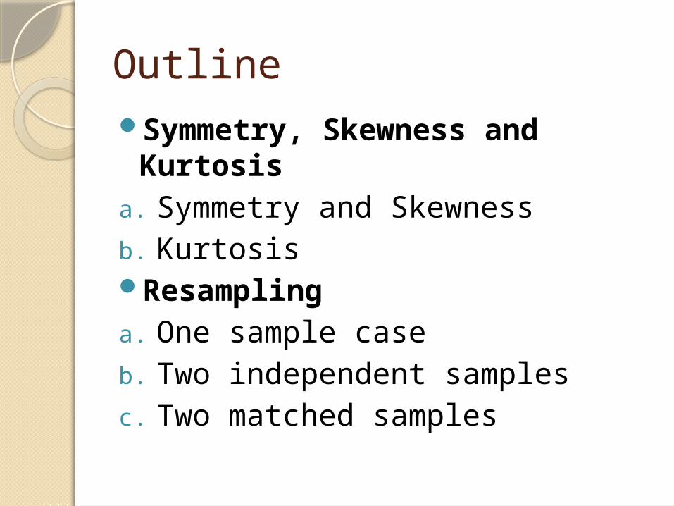
OutlineSymmetry, Skewness and

Kurtosisa. Symmetry and Skewnessb. KurtosisResamplinga. One sample caseb. Two independent samplesc. Two matched samples

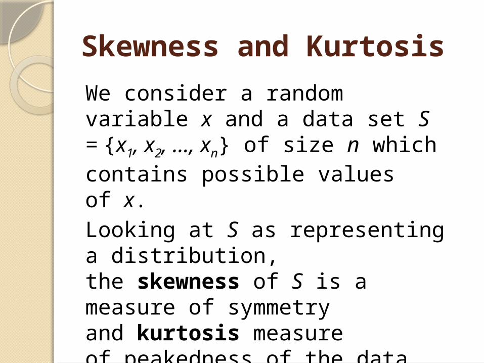
Skewness and KurtosisWe consider a random variable x and a data set S = {x1, x2, …, xn} of size n which contains possible values of x.Looking at S as representing a distribution, the skewness of S is a measure of symmetry and kurtosis measure of peakedness of the data in S.

Symmetry and SkewnessWe use skewness as a measure of symmetry. If the skewness of S = 0 then the distribution represented by S is perfectly symmetric.If the skewness is negative, then the distribution is skewed to the left, Contrary to the positive.

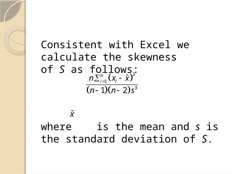
Consistent with Excel we calculate the skewness of S as follows:

where   is the mean and s is the standard deviation of S.

31

31 2

ni in x x

n n s

x

Observation: When a distribution is symmetric, the mean = median, when the distribution is positively skewed the mean > median and when the distribution is negatively skewed the mean < median.

Example: Suppose S = {2, 5, -1, 3, 4, 5, 0, 2}. The skewness of S = -0.43, i.e. SKEW(R) = -0.43 where R is a range in an Excel worksheet containing the data in S. Since this value is negative, the curve representing the distribution is skewed to the left (i.e. the fatter part of the curve is on the right). Also SKEW.P(R) = -0.34.

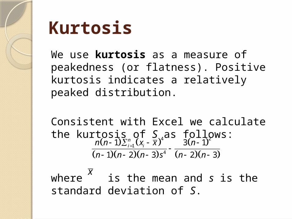
KurtosisWe use kurtosis as a measure of peakedness (or flatness). Positive kurtosis indicates a relatively peaked distribution.

Consistent with Excel we calculate the kurtosis of S as follows:

where   is the mean and s is the standard deviation of S.

4 21

4

1 3 11 2 3 2 3

ni in n x x n

n n n s n n

x

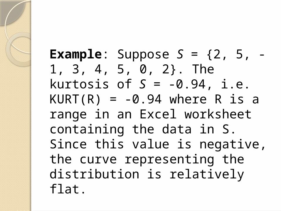
Example: Suppose S = {2, 5, -1, 3, 4, 5, 0, 2}. The kurtosis of S = -0.94, i.e. KURT(R) = -0.94 where R is a range in an Excel worksheet containing the data in S. Since this value is negative, the curve representing the distribution is relatively flat.

ResampleResampling procedures are based on the assumption that the underlying population distribution is the same as a given sample.

Resampling is useful when the population distribution is unknown or other techniques are not available.

We consider two types of resampling procedures: bootstrapping, where sampling is done with replacement, and permutation (also known as randomization tests), where all possible permutations of the data are made.

One sample caseExample 1.Calculate a 95% confidence interval around the median for the memory loss program described in Example 1 of the Sign Test, but with the data given in columns A and B of Figure 1.

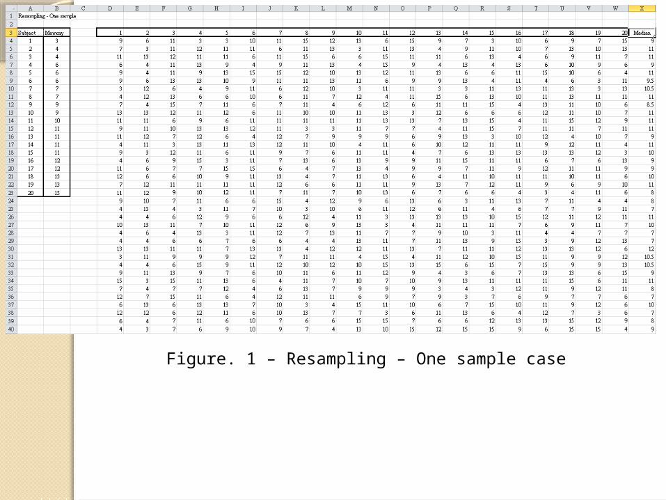
Figure. 1 – Resampling – One sample case

We treat the sample as the population and draw 2,000 samples of size 20 (the same size as the original sample) with replacement.

Referring to Figure 1, each element in each sample is selected using the following function:

=INDEX(B4:B23,RANDBETWEEN(1,20))

We now take the median of each of the 2,000 samples (only the first 21 samples are shown in Figure 1) and plot their distribution in a histogram. The results are displayed in Figure 2.

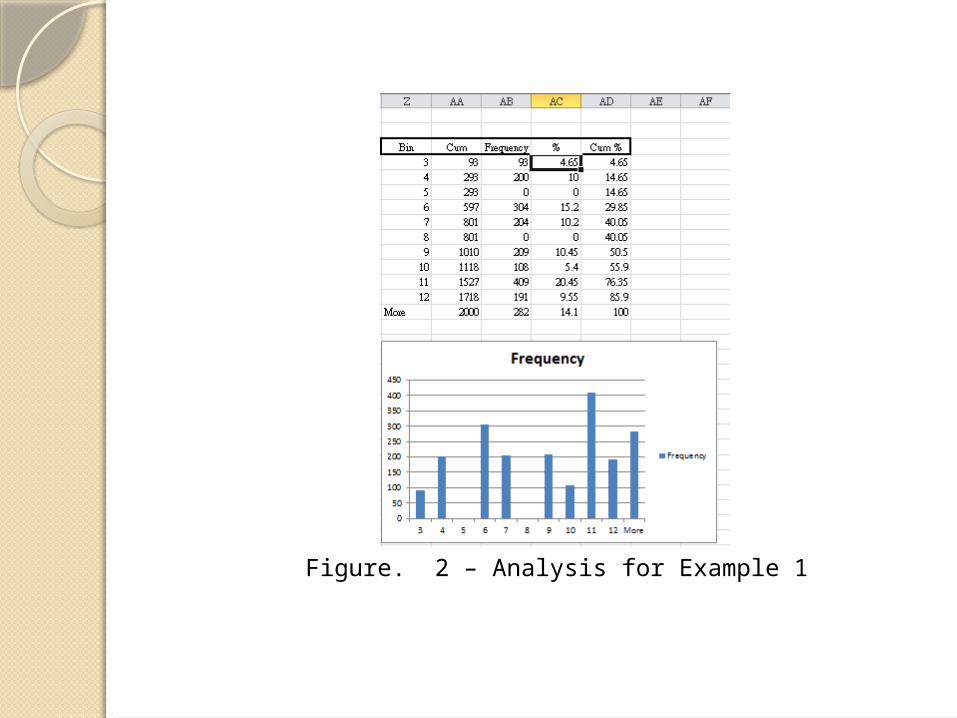
Figure. 2 – Analysis for Example 1

The value at the 2.5% percentile is 3 and the value at the 97.5% percentile is 13. Thus we can consider the confidence interval as [3, 13], which contains the sample median of 9.5.

Two independent samplesWe now consider the case where we have two independent samples. When the data is normally distributed, we would use the t-test.We can also use the Wilcoxon Rank Sum or Mann-Whitney non-parametric test. We now show how to address such problems using the permutation version of resampling.

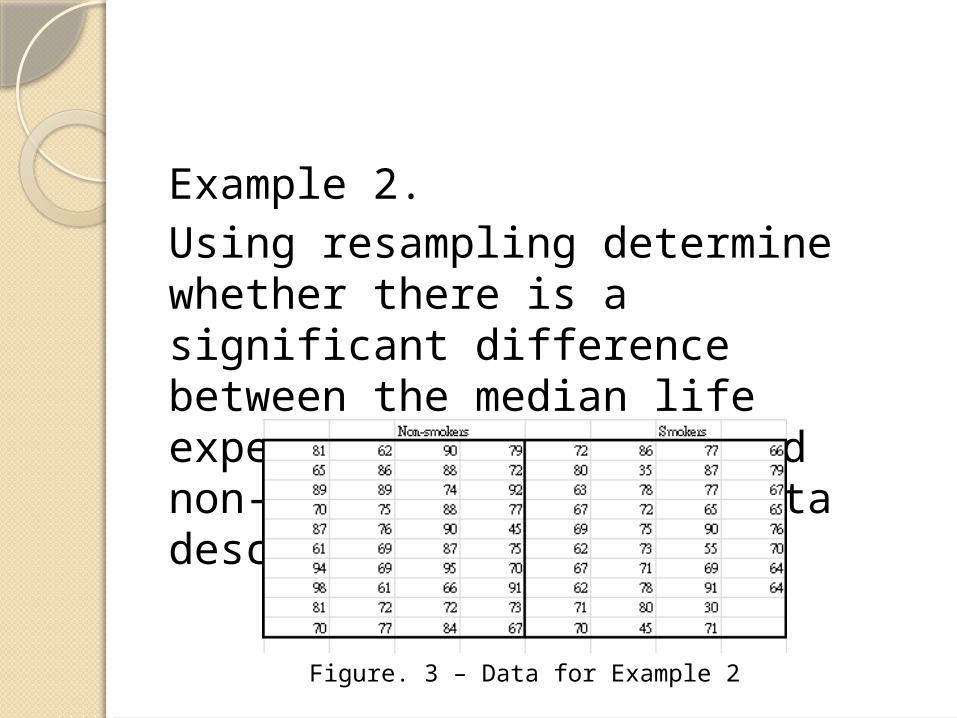
Example 2.Using resampling determine whether there is a significant difference between the median life expectancy of smokers and non-smokers using the data described in Figure 3

Figure. 3 – Data for Example 2

Note that the median score of the non-smokers is 76.5 while the median score of smokers is 70.5, a difference of 6.

The null hypothesis is that there is no difference between the two groups, i.e.

H0: the median score for the population of smokers and non-smokers are the same.

Based on the null hypothesis, we can assume that we have a single population of 78 . To test the hypothesis we take 2,000 random samples of size 78 from this population without replacement and assume that for each sample the first 40 scores come from the non-smokers and the remaining 38 come from the smokers.

We use formulas of form

=INDEX(J4:CI4,1,RANK(DC6,DC6:GB6))

where the range J4:CI4 contains all 78 data elements in the “population” and DC6:GB6 contains 78 random numbers, generated using RAND().For each of the 2,000 samples we calculate the median of the non-smokers and smokers and record the difference.

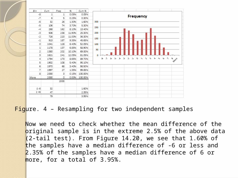
Figure. 4 – Resampling for two independent samples

Now we need to check whether the mean difference of the original sample is in the extreme 2.5% of the above data (2-tail test). From Figure 14.20, we see that 1.60% of the samples have a median difference of -6 or less and 2.35% of the samples have a median difference of 6 or more, for a total of 3.95%.

This means that the probability of getting a sample in either tail based on the null hypothesis is .0395 < .05 = α , and so we reject the null hypothesis and conclude with 95% confidence that there is a significant difference between the life expectancy of smokers and non-smokers.

Two matched samplesWe now consider the case where we have two matched samples.we would use the Paired Sample t-test. Even for non-normal data we can use the Wilcoxon Signed-Ranks non-parametric test.

Example 3: Using resampling determine whether there is a significant difference between the median life expectancy of smokers and non-smokers using the data described in Figure 3

The null hypothesis is there is no difference between the right and left eye’s ability to recognize objects, i.e. the median difference is zero.

If the null hypothesis is true then each of the 15 scores for the right eye is just as likely to be larger as smaller than the scores for the left eye.This is a form of sampling without replacement. The absolute values of the elements in each sample are as in the population, only the signs are variable.

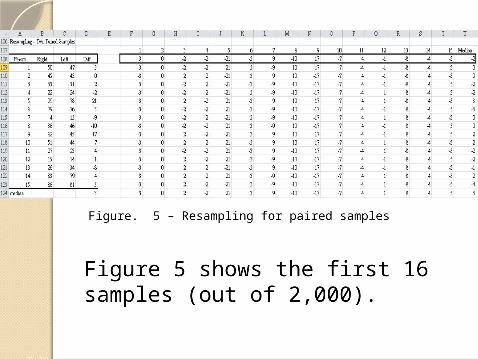
Figure 5 shows the first 16 samples (out of 2,000).

Figure. 5 – Resampling for paired samples

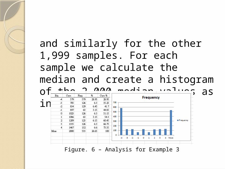
and similarly for the other 1,999 samples. For each sample we calculate the median and create a histogram of the 2,000 median values as in Figure 6.

Figure. 6 – Analysis for Example 3

The median of the original sample (i.e. the resampling “population”) is 3. From Figure 6 we see that 10.00% all the samples have a median ≤ -3 and 12.30% have a median ≥ 3. Since 10.00 + 12.30% = 22.30% ≥ 5% = α, we cannot reject the null hypothesis, and so conclude there is no significant difference between the right and left eye of the population.