Embed Size (px)
Citation preview
University of California, BerkeleyEE230 - Solid State Electronics Prof. J. Bokor
Transport Theory(read Lundstrom 3.1 - 3.4)
Aim Develop a general approach for relating microscopic description of carrier motion to mac-roscopic description.
Drift-Diffusion equation:
Classical approach to device design
material properties: μ , D +Boundary conditions
microphysics is buried devicein here structure
Device behavior described by independent specification of material and structure.
Modern devices
μ, D: can’t bury microphysics (i.e. ballistic transport)also depend explicitly on device structure (i.e. nonlocal transport)
Carrier energy & momentum distributions vary strongly in devices
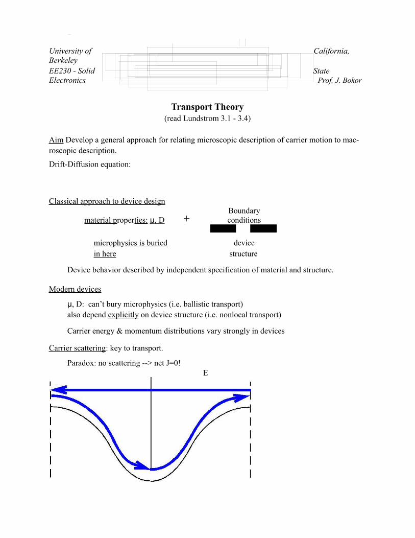
Carrier scattering: key to transport.
Paradox: no scattering --> net J=0!E
k
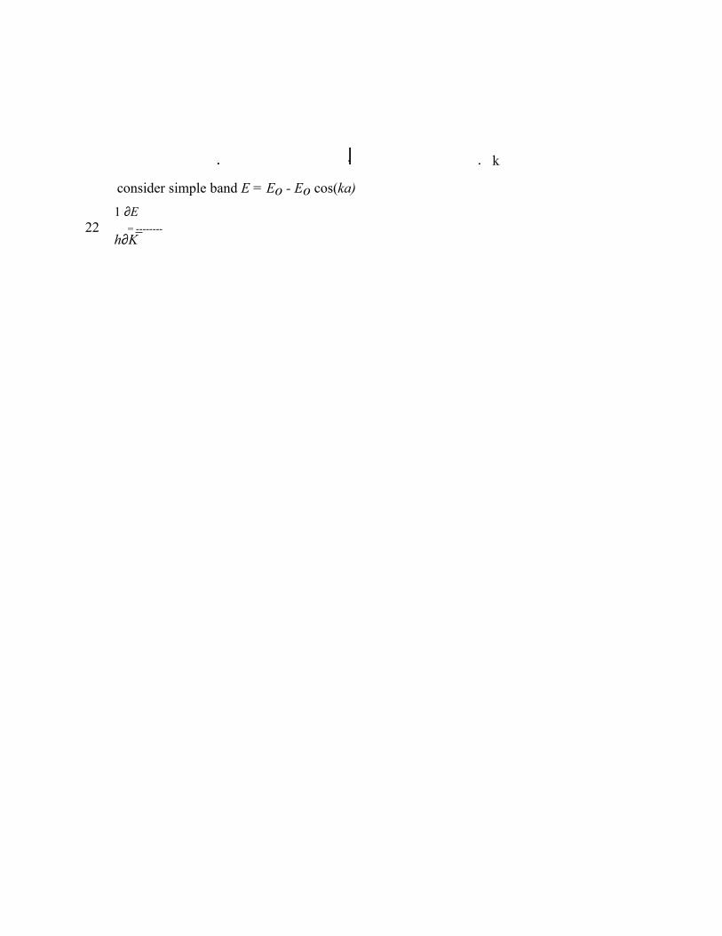
consider simple band E = Eo - Eo cos(ka)
1 ∂E 22 = --------
h∂K

=Eoa-------- sin( ka)
hBoltzmann equation Handout.fm
University of California, BerkeleyEE230 - Solid State Electronics Prof. J. Bokor
periodic motion - Bloch oscillation. This has been experimentally observed in superlattices [“Coherent submillimeter-wave emission from Bloch oscillations in a semiconductor super-lattice,” C. Waschke, et al., Phys. Rev. Lett. 70, 3319 - 3322 (1993). PDF copy is posted on the class web site.]
Electrons oscillate through BZ [Bragg diffraction] → localized in real space → no net cur-rent!
Scattering damps oscillation resulting in a net motion in an applied field. Yet the motion is damped by scattering. The message is that transport depends on the balance between the applied driving force and dissipation by scattering forces.
Boltzmann transport equation
Semi-classical approach. In semiconductors, all the QM is buried in m*. Electron motion will be described by classical mechanics, except that scattering probabilities will also be derived using quantum mechanics.
Complete description: could solve Newton equations for each particle (electron):
dpi ( , , )
------- = qE + F r p t dt
random forces due to phonons, impurities
for all i = 1, …, N . This is clearly not feasible.
Instead, we take a statistical approach:define distribution function (single particle):
f(r, p, t): probability of finding a particle at r , with momentum p at time t.
“phase space”: 6 dimensional space - x, y, z, px, py, pz
The particle density is found as:
Since momentum is discrete, we show a summation over allowed values of p. However, it is

- 93 -
University of California, BerkeleyEE230 - Solid State Electronics Prof. J. Bokor
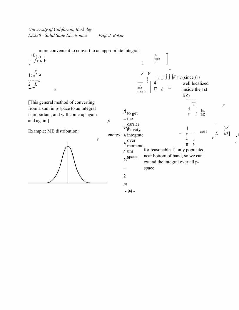
more convenient to convert to an appropriate integral.1
∑ ( , ) →
-- f r p V
p
12 π 3
-- -----h 2 L
≅
1 ⁄ V
vol----------
------of
---
one state in
p-space
13
∞
_3 ∫ ∫ ∫f( r, p4π h
–∞
(since f is well localized inside the 1st BZ)
[This general method of converting from a sum in p-space to an integral is important, and will come up again and again.]
Example: MB distribution:
f
p
energy
f(
=
exp
E
E
⁄
kT
–
2
m
to get the carrier density, integrate over momentum space
--------------
F4π
3 _3
h1st BZ
=1
– E
) ⁄ kT]
∫e
-------------- exp[ ( E
F4π
_3
hfor reasonable T, only populated near bottom of band, so we can extend the integral over all p-space
- 94 -
University of California, BerkeleyEE230 - Solid State Electronics Prof. J. Bokor
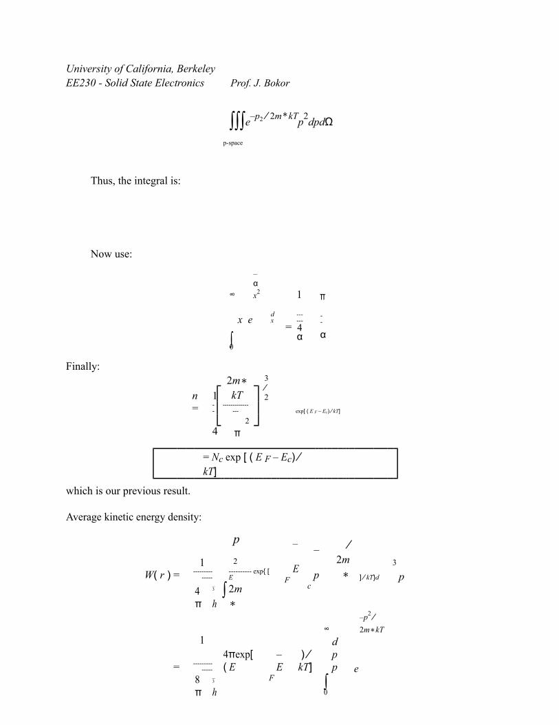
∫∫∫e–p2
⁄ 2m∗kT
p2dpdΩ
p-space
Thus, the integral is:
Now use:
∞
–α
x2 1 π
∫
x e=
dx
------
--
4α α
0
Finally:
n =
1
2m∗
kT
3 ⁄ 2
--
---------------- exp[ ( E F – Ec) ⁄ kT]
4 π2
= Nc exp [ ( E F – Ec) ⁄ kT]
which is our previous result.
Average kinetic energy density:
W( r ) =1
∫
p
2
– E
– p
⁄ 2m∗
3
p---------
--------------- exp{ [ E F
c] ⁄ kT}d
4π
_3 2m
∗h
1∞
–p2 ⁄
2m∗kT
=4πexp[ ( E
– E
) ⁄ kT]
∫
dpp e
--------------
F8π
_3
h 0
31 ⁄ 2 ∗
5 ⁄ 2
--π ( 2 m kT)
8
3 1
2 m∗kT
3 ⁄ 2
=--
---------------- exp[ ( E
– E ) ⁄ kT]-- kT
F2 4 _2
πh
- 95 -
University of California, BerkeleyEE230 - Solid State Electronics Prof. J. Bokor
W 3So we can say that the energy / electron = ---- = --kT . Again, a familiar result.
n 2
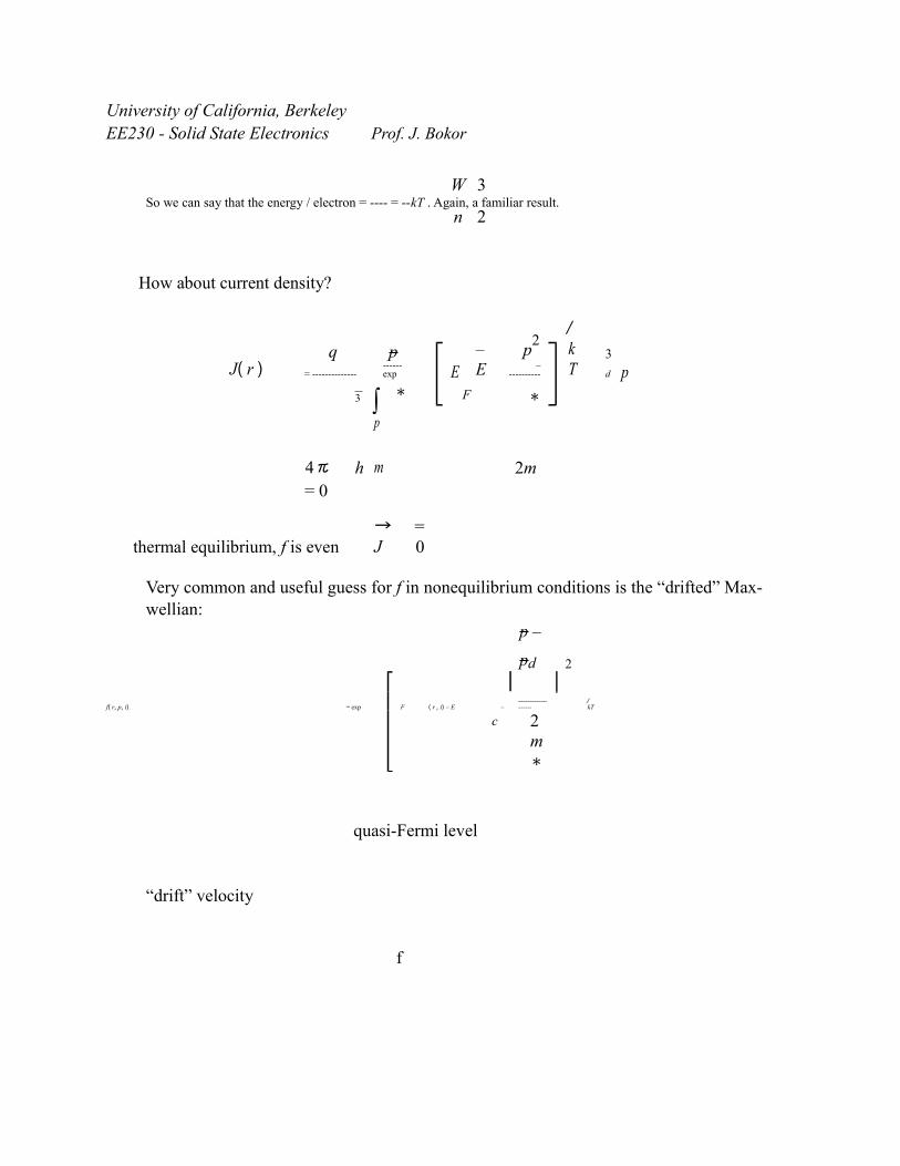
How about current density?
J( r )q
∫
pE
– E
p2
⁄ kT
3
p= -------------------- exp
F
– ---------- d
_3 ∗ ∗
4π h
p
m 2m
= 0
thermal equilibrium, f is even→ J
= 0
Very common and useful guess for f in nonequilibrium conditions is the “drifted” Max-wellian:
p –
pd 2
f( r, p, t) = exp F ( r , t) – E
c–
-------------------
⁄ kT
2m∗
quasi-Fermi level
“drift” velocity
f
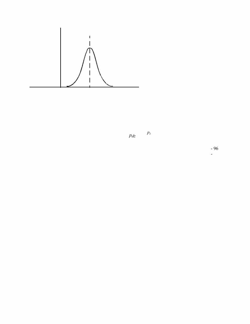
pdzpz
- 96 -
University of California, BerkeleyEE230 - Solid State Electronics Prof. J. Bokor
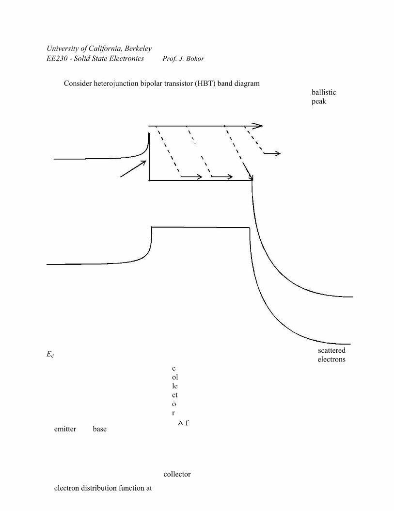
Consider heterojunction bipolar transistor (HBT) band diagram
Ec
ballistic peak
scattered electrons
emitter base
collector
electron distribution function at
collector
f
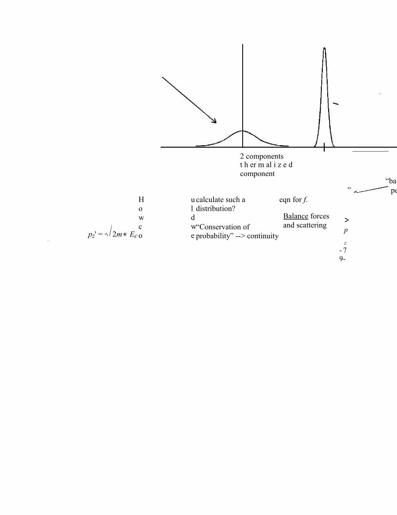
2 componentst h er m al i z e dcomponent
“ballistic” peak
pz' = 2m∗ Ec
How co
uld we
calculate such a distribution?
“Conservation of probability” --> continuity
eqn for f.
Balance forces and scattering
p
z
- 9
7 -
University of California, Berkeley
EE230 - Solid State ElectronicsProf. J. Bokor
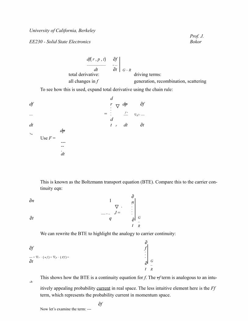
df( r , p , t) ∂f---------------------- = ---
dt ∂t G – Rtotal derivative: driving terms:
all changes in f generation, recombination, scattering
To see how this is used, expand total derivative using the chain rule:
df
=
dr ∇ dp ∂f
----
----
f + ----- ∇pf + ----
dtdt r dt ∂t
dp
Use F = ----- . dt
This is known as the Boltzmann transport equation (BTE). Compare this to the carrier con-tinuity eqn:
∂n 1∇ ⋅ J =
∂n
----- + --
-----
∂t q ∂t
G – R
We can rewrite the BTE to highlight the analogy to carrier continuity:
∂f∂f
--- + ∇r ⋅ ( v f ) + ∇p ⋅ ( Ff ) =
---
∂t ∂t
G – R
This shows how the BTE is a continuity equation for f. The vf term is analogous to an intu-
itively appealing probability current in real space. The less intuitive element here is the Ff
term, which represents the probability current in momentum space.
∂fNow let’s examine the term: ---
∂t G – R
2 processes contribute.1. Actual generation-recombination processes such as photogeneration, defect recombination, stimulated emission, ...
explicitly write s(r, p, t) for these
2. Carrier scattering . This takes carriers from one momentum state to another - creates sources-sinks in momentum space.
- 98 -
University of California, Berkeley
EE230 - Solid State ElectronicsProf. J. Bokor
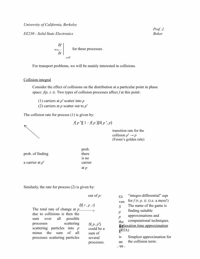
∂ffor these processes.Write ---
∂tcoll
For transport problems, we will be mainly interested in collisions.
Collision integral
Consider the effect of collisions on the distribution at a particular point in phase space: f(p, r, t). Two types of collision processes affect f at this point:
(1) carriers at p′ scatter into p (2) carriers at p scatter out to p′
The collision rate for process (1) is given by:
f( p ′)[ 1 – f( p )]S( p ′, p)
prob. of findingprob. there
a carrier at p′is no carrierat p
Similarly, the rate for process (2) is given by:
transition rate for thecollision p′ → p(Fermi’s golden rule)
The total rate of change at p due to collisions is then the sum over all possible processes scattering scattering particles into p minus the sum of all processes scattering particles
out of p:
∂f( r , p , t)----------------------∂t
S( p, p′) could be a sum of several processes.
Given Sppthe BTE is an
“integro-differential” eqn for f (r, p, t). (i.e. a mess!) The name of the game is finding suitable approximations and computational techniques.
Relaxation time approximation (RTA)
Simplest approximation for the collision term:
- 99 -
University of California, BerkeleyEE230 - Solid State Electronics Prof. J. Bokor
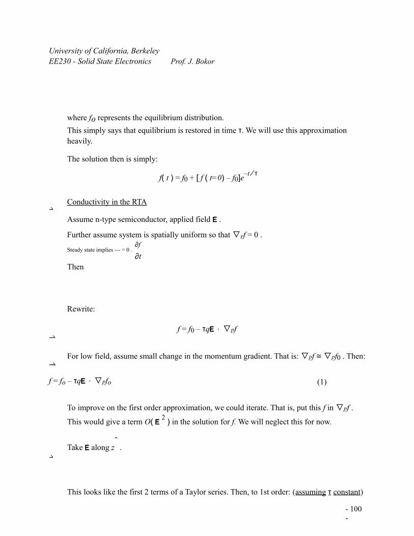
where fo represents the equilibrium distribution.
This simply says that equilibrium is restored in time τ. We will use this approximation heavily.
The solution then is simply:
f( t ) = f0 + [ f ( t=0) – f0]e–t
⁄ τ
Conductivity in the RTA
Assume n-type semiconductor, applied field E .
Further assume system is spatially uniform so that ∇rf = 0 .∂f
Steady state implies --- = 0 .∂t
Then
Rewrite:
f = f0 – τqE ∇⋅ pf
For low field, assume small change in the momentum gradient. That is: ∇pf ≅ ∇pf0 . Then:
f = fo – τqE ∇⋅ pfo (1)
To improve on the first order approximation, we could iterate. That is, put this f in ∇pf .
This would give a term O( E 2 ) in the solution for f. We will neglect this for now.
Take E along zˆ .
This looks like the first 2 terms of a Taylor series. Then, to 1st order: (assuming τ constant)
- 100 -
University of California, BerkeleyEE230 - Solid State Electronics Prof. J. Bokor
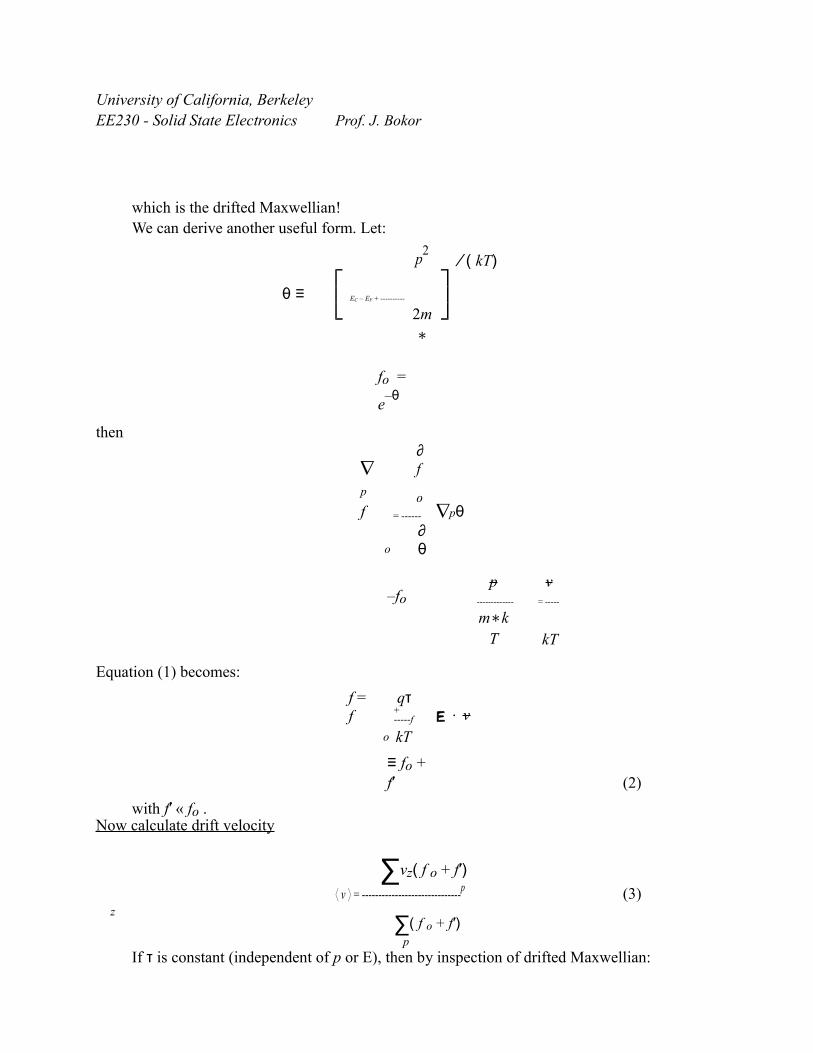
which is the drifted Maxwellian!We can derive another useful form. Let:
θ ≡
p2
⁄ ( kT)
EC – EF + ----------
2m∗
fo =
e–θ
then
∇
p
f
∂f
o∇pθ
o
= ------
∂θ
–fop v
------------- = -----
m∗kT kT
Equation (1) becomes:
f = f
qτE ⋅ v
o
+ -----f
kT
≡ fo + f′ (2)
with f′ « fo .Now calculate drift velocity
∑vz( f o + f′)
⟨ v ⟩ = ------------------------------p (3)
z∑( f o + f′)
p
If τ is constant (independent of p or E), then by inspection of drifted Maxwellian:

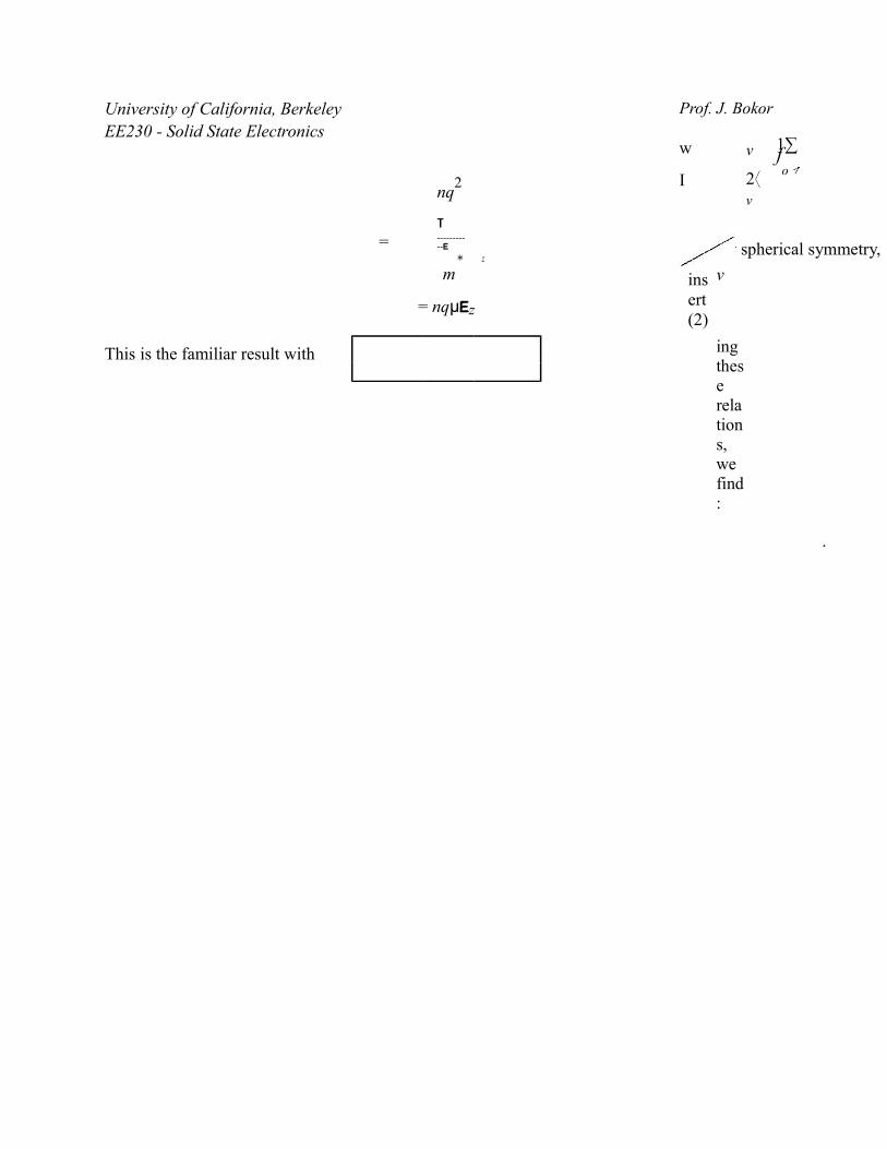
Current density is given by:
- 101 -
University of California, BerkeleyEE230 - Solid State Electronics
=
nq2
τ-----------E
z∗
m
= nqμEz
This is the familiar result with
Prof. J. Bokor
w
I
v
2⟨v
1∑fo
insert (2)
By spherical symmetry,
v
ing these relations, we find:
.
University of California, BerkeleyEE230 - Solid State Electronics
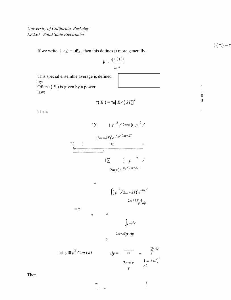
If we write: ⟨ v z⟩ = μEz , then this defines μ more generally:
μq ⟨ ⟨ τ ⟩⟩
= ---------------- .
m∗
This special ensemble average is defined by:Often τ( E ) is given by a power law:
τ( E ) = τ0[ E ⁄ ( kT)]s
Then:
1∑ ( p 2 ⁄ 2m∗)( p
2 ⁄
2m∗kT)se
–p2 ⁄ 2m∗kT
2⟨ ⟨ τ⟩⟩ =
τ0-------------------------------------------------------------------------------------------p
1∑ ( p 2 ⁄
2m∗)e–p2 ⁄ 2m∗kT
∞
∫( p 2 ⁄ 2m∗kT)se
–p2 ⁄
2m∗kTp
4dp
= τ------------------------------------------
--------------------------------0
∞0
∫e–p2 ⁄
2m∗kTp4dp0
let y ≡ p2 ⁄ 2m∗kT dy =
----------------2pdp =
--------------------
2y1 ⁄
2
2m∗kT
( m ∗kT)1
⁄ 2
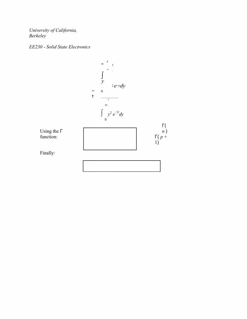
Then
∞ 1
s –--
⟨ ⟨ τ⟩⟩ = τ
- 103 -
University of California, Berkeley
EE230 - Solid State Electronics
∞s +
3
--
∫y
2 e–ydy= τ
0
----------------------------
∞
3
∫
--
0y2 e
–ydy
Using the Γ function:
Γ( n )
Γ( p + 1)
Finally:

- 104 -