Embed Size (px)
Citation preview

BRAKE SYSTEM PERFORMANCE EVALUATION OF FORMULA TYPE VEHICLE
Felipe Mestre1, Kaue B. Pironato1, Romulo M. Silva1, Paulo Lee1, Sergio K. Moriguchi1,
Fernando Malvezzi1
1 Maua Institute of Technology
E-mails: author 5: [email protected], author 6: [email protected]
ABSTRACT
Formula Student and Formula SAE are student competitions where engineering students must
develop a Formula type vehicle according to a series of rules. Regarding to the brake system,
these rules determine some requirements that the cars must be in accordance.
This work deals with a performance evaluation of brake system of Formula type vehicle.
First, a mathematical model was developed to achieve the balance of front and rear braking
forces. This model takes into account the most important vehicle parameters that influence
braking performance, as well as the tire/road friction conditions. Then, the results obtained
from the model were compared against experimental data. During the tests the vehicle
velocity, the lateral and longitudinal vehicle acceleration and the circuit pressure to the front
and rear brakes were monitored. This mathematical model will be employed to development
of brake systems to be applied to Formula type vehicle.
Finally, a second experimental test was employed to evaluate the brake system performance
considering the vehicle operating in competition conditions.
The obtained results show that the mathematical model is suitable for brake system
performance prediction. Moreover, the tests results show that the brake system is suitable
under competition conditions.
INTRODUCTION
The Formula SAE is a student competition organized by SAE International in which
engineering students design and built a Formula type vehicle which is evaluated by a variety
of static and dynamic events.
Regarding to the brake system, the Formula Student rules is similar to the SAE ones. These
rules determine that the cars must be equipped with a braking system operated by a single
control that acts on all four wheels. This system must have two independent hydraulic circuits
such that in the case of failure at any point in the system, effective braking power is
maintained on at least two wheels. The brake system must be capable to lock all four wheels
during the specific test. “Brake-by-wire” systems are prohibited. The brake pedal must be
designed to resist a force of 2000 N without any failure of the brake system or pedal box
[1,2].
The braking system is important not only for the safety but also for performance of racing
cars [3]. An efficient brake system should achieve the maximum longitudinal force available
in tire-pavement contact.

According to Canale [4], the longitudinal force is caused by the tire deformation. The
compressed fibers of tire expand so there is a relative slipping over the ground surface that
creates the longitudinal force. The maximum value of this force in passenger vehicle tires is
achieved when relative slip reaches the range from 10% to 20%.
According to Gillespie, adhesion and hysteresis are the primary mechanisms for friction
coupling [5]. These mechanisms depend on small amount of slip that occurs at the tire-
pavement contact.
In order to define the braking systems parameters, models for brake balance analysis have
been employed. Limpert presented a vehicle braking dynamic model in which both
aerodynamic and driveline drags are neglected [6]. Breuer and Bill show a braking dynamic
model specific for race car in which the aerodynamic effects are taken into account but the
engine torque during the braking maneuver is not considered [7].
Some works have presented Formula SAE braking development. Heffernan introduced an
analytical technique for performing brake rotor temperature analysis using empirical data [8].
It can be useful to predict fading problems when the design disc brake system is developed.
Schommer et al. have applied a combination of topology optimization and Direct Metal Laser
Sintering to manufacture of a FSAE brake caliper [9]. The results based on the thermal
simulations showed that the new caliper achieved heat transfer improvements, and maintained
a considerable stiffness.
This paper presents a brake system performance evaluation of Formula SAE type vehicle. A
mathematical model was developed to know the balance of front and rear braking forces. In
addition, an experimental test was employed to evaluate the brake system performance
considering the vehicle operating in competition conditions.
1. BRAKE SYSTEM
The brake system of this work has got a disc brake in all of four wheels, with hydraulic drive
and without assistance. The brake pedal activates two independent master cylinders, one to act
on the front wheels and the other one to act on the rear wheels (Fig. 1-a).
(a)
(b)
(c)
Figure 1. (a) Disc brake and caliper; (b) Brake bias; (c) Dial

A brake bias system is used to control force distribution generated by the pedal between the
two master cylinders (Fig. 1-b). The driver can adjust the brake balance via a dial located in
the cockpit (Fig. 1-c).
Therefore, the balancing of the braking forces between the front and rear axles is achieved by
the pressure difference between the front and rear circuits. The brake bias system allows using
the same wheel cylinders and the same disc brakes on both axles, reducing the number of
components types.
2. MODELING AND BRAKE BALANCE ANALYSIS
The forces responsible to generate vehicle deceleration are originated not only by the braking
forces but also by the tire rolling resistance, aerodynamic drag, driveline inertia effects and
driveline drag.
Only the forces generated by the brake system are considered in the analysis developed in this
work. The approach presented here is based on Limpert work [6]. This analysis considers both
the optimum braking forces and the actual braking forces.
The vehicle parameters employed in this work are presented in the Appendix.
2.1. Optimum Braking Force
The optimum braking force distribution is achieved when all wheels reach the imminent
locking simultaneously [5, 6, 10]. The model developed to calculate these forces take into
account the following hypothesis: both the tire rolling resistance and the aerodynamic drag are
neglected; the braking occurs only in straight line and with uncoupled transmission; the tires
are on the imminence of locking during braking and the wheel moment of inertia is negligible.
Although the vehicle analyzed in this work is a single seater race car, it is not equipped with
wings and during competitions the velocity usually is lower than 75 km/h.
Figure 2. Forces acting on vehicle during braking
Appling the Newton-Euler equations for the system of Fig. 2 one obtains:
(1)
(2)

(3)
Where:
: front axle vertical load
: rear axle vertical load
: vehicle mass (driver included)
: gravitational acceleration
: distance between front axle and gravitational center
: wheel base length
: gravitational center height
: longitudinal deceleration
: tire/road adhesion coefficient
The optimum front and rear braking forces are obtained by applying equations (4) and (5),
respectively:
.
(4)
(5)
Where:
Fxf : front axle braking force
Fxf: rear axle braking force
The forces Fxf and Fxr can be expressed relative to vehicle weight by dividing the braking
forces Fxf and Fxr by vehicle weight. Moreover, substituting equation (3) in equations (1) and
(2) we obtain:
.
(6)
(7)
Adopting values between 0 and 1.4 for the tire/road adhesion coefficient equations (6) and (7)
lead to the graph showed in Fig. 3. As different drivers can drive the car during competition,
Fig. 3 presents two optimum curves for two different vehicle gravitational center positions.

0 0.2 0.4 0.6 0.8 1 1.2 1.4
0
0.2
0.4
0.6
Normalized front axle braking force
No
rma
lize
d r
ea
r a
xle
bra
kin
g fo
rce
Optimum braking force distribution (First CG position)
Optimum braking force distribution (Second CG position)
Constant deceleration lines
Figure 3. Optimum normalized braking forces
2.2. Actual Braking Force
The actual braking force modelling was developed to determine the front and rear axle
braking force. These real forces were compared to the optimum braking forces to evaluate the
installed braking system efficiency.
The brake pedal force is distributed between the front and rear master cylinders through a
device called brake bias (brake balance), which allows the driver to control the distribution of
braking forces between the front and rear axles in order to maximize overall brake balance
during competition.
Figure 4. Brake pedal dimensions
The pressures generated by the front and rear master cylinders are determined by the
equations (8) and (9), respectively.
(8)
(9)

Where:
pf : front brake circuit pressure
pr : rear brake circuit pressure
Fp : pedal force
AMf: effective area of front master cylinder
AMr : effective area of rear master cylinder
ip : pedal ratio (ℓ1/ℓ2)
ℓ1 : distance from foot to pedal pivot (Fig. 4)
ℓ2 : distance from pushrod to pedal pivot (Fig. 4)
β : brake bias ratio (front-to-rear)
The brake system of this work is floating caliper disc brake. At this system, the torque applied
to the disc brake is obtained by equation (10).
(10)
Where:
Tdisc : torque applied to each disc brake
µpad : pad/disc brake coefficient of friction
Rc : effective radius disc brake
p: brake circuit pressure
Ac : caliper piston area
Neglecting the inertia moment of wheels, the front axle braking force at straight-line braking,
expressed in reference to vehicle weight is:
(11)
In the same conditions, the rear axle braking force expressed in reference to vehicle weight is:
(12)
Where:
p0 : pushout pressure

C*: brake factor (2μpad)
Rt: tire rolling radius
η: wheel cylinder efficiency
Acf : front caliper piston area
Acr: rear caliper piston area
Rcf : front disc effective radius
Rcr: rear disc effective radius
Considering a pedal force of 425 N, a brake bias ratio equal to 71.5% and applying Eq. (8),
(9), (11) and (12), one obtains the actual braking force distribution, as shown in Fig. 5. The
optimum braking force curve intersects the actual braking force line when the vehicle
achieves a deceleration equal to 1.0g. If the maximum tire/road adhesion coefficient is
achieved when the vehicle deceleration is equal to 1.0g, there will be a simultaneous locking
of the four wheels. When decelerations are higher than 1.0g, the locking of rear axle will
occur first. On the other hand, when decelerations are lower than 1.0g, the locking of front
axle will occur first.
0 0.2 0.4 0.6 0.8 1 1.2
0
0.2
0.4
Normalized front axle braking force
No
rma
lize
d r
ea
r a
xle
bra
kin
g fo
rce
Optimum braking force distribution
Actual braking force distribution (Bias ratio: 71.5%)
Constant deceleration lines
Figure 5. Actual and optimum braking force distribution (driver mass of 78 kg)
Figure 6 represents the optimum and the actual braking force distribution referred to the
operating range of the brake bias. This range is sufficient for the drivers to achieve the
optimum brake balance during competition.

0 0.2 0.4 0.6 0.8 1 1.2 1.4
0
0.1
0.2
0.3
0.4
0.5
0.6
0.7
Normalized front axle braking force
No
rma
lize
d r
ea
r a
xle
bra
kin
g fo
rce
Optimum braking force distribution (First CG position)
Optimum braking force distribution (Second CG position)
Actual braking force distribution (Bias ratio: 50%)
Actual braking force distribution (Bias ratio: 80%)
Constant deceleration lines
Figure 6. Normalized optimum and actual braking force distribution
2.3. Pedal Force Gain
In order to evaluate the pedal force during braking, the pedal force gain was calculated, which
is the relation between pedal force and vehicle deceleration [5]. According to the model
prediction, the required pedal force to the vehicle achieves a deceleration of 1.0g is 425 N,
considering a mass of the driver equal to 78 kg. For a driver mass of 60 kg, this force is 404 N
and for 90 kg the force is 438 N. These values were compared to NHTSA research, which has
identified an optimum range for pedal force gain, as seen in Fig. 7. As there is no specific
reference for formula cars type, a NHTSA recommendation developed for passenger was used
for the single seater race car of this study. The red points in Fig. 7 represent the pedal force
gain for the three drivers.
Figure 7. Pedal Force Gain – according to NHTSA shaded area represents the optimum gain

3. TESTS PROCEDURE
Two tests were performed to evaluate the brake system. In the first one, the results obtained
with the mathematical model were compared to collected data during experimental tests to
evaluate this model. The second test analyzed the performance of the braking system in a
competition circuit. Both tests were monitored by sensors to measure the pressure on the front
and rear lines of the brake system, the longitudinal and lateral acceleration and the velocity of
the vehicle.
Figure 8. Sensors assembling
Figure 8 presents the connection of the inlet (A) with the outlet for each wheel cylinder (B)
and the pressure sensor (C). When the brake pedal is pressed, the system is pressurized by the
brake fluid and the sensor performs the pressure reading, sending the data to the AIM® data
acquisition system.
The longitudinal and lateral vehicle accelerations were obtained via an accelerometer
assembled near to the center of gravity of the vehicle.
The track and velocity of the vehicle were obtained via GPS-Global Position System. In
addition, the GPS was employed to identify the braking points presented in Figure 9.
The setting of brake bias employed during the tests was determined by equation (13).
(13)
3.1. Comparison of model and track test results
The test to evaluate the model accuracy was performed on a flat and dry asphalt racetrack.
This test procedure was based on accelerated the vehicle up to the reference speed of 60 km/h.
After that, the car was braked in straight-line and without motor action (acting on the brake
pedal and clutch simultaneously) until it stopped completely. Right after the car stopped
completely, the temperatures of the four brake pads were measured.
Tests were performed at different positions of brake bias. In all of the tests, the driver applied
a “soft” force on the brake pedal. Then, these procedures were repeated with a “strong”
intensity braking. Table 1 shows the vehicle parameters and weather conditions during model
evaluation test.

Table1. Vehicle parameters and weather conditions during model validation test
Vehicle parameters/
weather conditions
Values
Asphalt temperature Between 26ºC and 40 ºC
Initial temperature of tires 23 ºC
Initial temperature of pads 25 ºC
Air temperature 28 ºC
Tire inflation pressure (cold tire) 13 psi (90 kPa)
Camber (front and rear wheels) 0o
Toe (front and rear wheels) 0o
3.2. Performance test of brake system at a competition circuit
Performance tests were conducted on the ECPA (a private racing circuit in Sao Paulo-Brazil),
in dry asphalt racetrack. As the tests evaluated the performance of the brake system in race
conditions, the driver did not activate the clutch during braking. Moreover, the driver actuated
on the brake pedal in turns, which influenced the maximum tire longitudinal force due to the
lateral acceleration effects [11].
Table 2 shows the vehicle parameters and weather conditions during competition circuit test.
Table 2. Vehicle parameters and weather conditions during competition circuit test
Vehicle parameters/
weather conditions
Values
Asphalt temperature Between 28ºC and 40 ºC
Initial temperature of tires 24 ºC
Initial temperature of pads 26 ºC
Air temperature 32 ºC
Tire inflation pressure (cold tire) 13 psi (90 kPa)
Front wheels camber -2o
Rear wheels camber 0o
Toe (front and rear wheels) 0o
4. TESTS RESULTS
4.1. Results obtained from model evaluation test
In the mathematical model evaluation test, two longitudinal accelerations were compared: one
from the vehicle braking and the other one obtained from the model.
As it was not possible to determine the force applied on the pedal by the driver during the test
(in real time), the measured pressure values obtained by the test were used into the equations
(11) and (12). Then, the vehicle deceleration was calculated by summing the values calculated
from equations (11) and (12).
Table 3 shows front and rear pressure circuits and longitudinal vehicle deceleration obtained
during tests. The graphs with all collected data are presented in the Appendix. In addition,

Table 3 shows a comparison between the values of deceleration obtained from the model and
the values measured during the tests. The experimental data collected during the tests were
disregarded when the lateral accelerations were higher than 0.10g, the longitudinal
decelerations were lower than 0.35g or higher than 1,50g.
Table 3. Pressure lines and longitudinal vehicle deceleration
Test
Front Line
Pressure
(MPa)
Rear Line
Pressure (MPa)
Actual
deceleration
(g)
Model
deceleration
(g)
Error
(%)
1 5.54 4.44 1.03 1.16 12.60
2 7.92 5.62 1.48 1.57 6.08
3 4.38 3.00 0.95 0.86 9.47
4 3.12 1.86 0.58 0.58 0
5 3.13 1.61 0.62 0.55 11.29
6 2.08 1.00 0.38 0.36 5.26
The disc brake temperature was monitored and measured at the end of braking. Table 4 shows
the temperature of disc brake immediately after the braking.
Table 4. Disc brake temperature (oC)
Test Right
Front
Left
Front
Right
Rear
Left
Rear
Brake Bias
(%)
1 131 135 123 126 55.5
2 142 157 103 113 58.5
3 86 93 72 70 59.3
4 74 77 65 72 62.6
5 130 124 91 97 66.0
6 88 91 79 73 67.5
The maximum temperature reached during the test was 157°C, which does not generate loss
of braking efficiency due to fading effect. The recovering time of the system up to the initial
temperature (about 40°C) measured after the vehicle has stopped was from 10 to 20 seconds.
To avoid reading error due to rapid recovery of the system, the temperature measurements
were performed immediately after vehicle has stopped.
4.2. Results obtained from race test
Figure 9 shows the competition circuit where the tests were carried out. The numbers indicate
the track sections where the driver was acting on the brake pedal.

Figure 9. Braking points during the test
Several laps were completed by the driver. The results of one of than are presented below.
In the figure 10 the curve highlighted in red represents the pressure inside the front brake line
and the blue curve represents the pressure inside the rear line of the brake circuit. In this lap,
initially the brake bias was set of 65-35, which means 65% braking force to the front wheels
and 35% to the rear axle.
Figure 10. Pressure inside the front (red line) and rear (blue line) brake circuits
The values of front and rear line pressures obtained during tests were employed to verify the
setting of brake bias, which was determined by the equation (13). Table 5 shows the results
for each braking point presented in Figures 10 and 11.

Table 5. Front and rear brake pressure
Track Section
(see Fig. 9) Total Pressure
(MPa) Front Pressure
(MPa) Rear Pressure
(MPa) % Front % Rear
1 4.87 3.05 1.82 63% 37%
2 7.13 4.64 2.49 65% 35%
3 5.38 3.51 1.87 65% 35%
4 6.04 3.84 2.20 64% 36%
5 3.47 2.34 1.13 67% 33%
6 6.38 3.89 2.49 61% 39%
7 4.56 2.93 1.63 64% 36%
8 2.25 1.60 0.65 71% 29%
Figure 11 shows the total brake pressure (obtained by adding the front and rear pressures), the
vehicle longitudinal velocity and the longitudinal acceleration of the vehicle. The numbers
correspond to the track section where the driver was acting on the brake pedal (see Figure 9).
The vehicle reached its maximum lap velocity of 74.6 km/h in track section number 2 and in
track section number 6 its maximum longitudinal acceleration of 1.22 g.
When the car was in track section number 2, the pressure of brake circuit reached its peak
value of 7.13 MPa (71.3 bar). Exactly when the brake pressure achieved that peak, the
longitudinal acceleration was equal to 1.06 g and immediately arose to 1.21 g.
Figure 11. Vehicle Speed, Longitudinal Acceleration and Total Pressure inside the brake circuits
Table 6 shows the values of velocity, longitudinal and lateral acceleration of the vehicle at the
exact instant when the brake pressure achieved the peak in each track section shown in Figure
9. Note that the peak of longitudinal acceleration did not occur at the exact moment when the
brake pressure achieved its maximum value, what can be observed in Figure 11.

Table 6. Vehicle Velocity, Longitudinal and Lateral Acceleration
Track Section
(see Fig. 9) Lateral
Acceleration (g) Longitudinal
Acceleration (g) Velocity (km/h)
1 0.56 0.77 62.1
2 0.70 1.06 72.5
3 0.74 0.78 47.4
4 0.01 0.85 63.6
5 1.06 0.71 54.2
6 0.42 0.77 58.6
7 -0.64 0.54 38.8
8 1.14 0.82 43.8
CONCLUSION AND COMENTS
In this paper, a brake system performance of a formula type vehicle was evaluated by both a
mathematical model and an experimental test. The model was useful to analyze the braking
forces distribution between the front and rear axles and to determine the suitable brake bias
ratio for the vehicle to achieve the optimum brake forces balance. Moreover, the range of
brake bias is good for the vehicle to reach the optimum braking performance with different
drivers who will drive the car during competition.
The results obtained in the model evaluation test show that the mathematical model is suitable
for brake system performance prediction. The maximum difference between the results of the
model and the results of the tests is lower than 13%. Moreover, while braking only in straight
line, the maximum vehicle longitudinal deceleration was equal to 1.48g.
Finally, the tests in competition circuit show that the brake bias ratio is suitable under
competition conditions. When braking in a turn, the vehicle achieves simultaneously
longitudinal deceleration of 1.06g and lateral acceleration of 0.7.
The future work will concentrate on simulation and experiments considering the aerodynamic
drag and downforce effects during braking.
ACKNOWLEDGEMENTS
The authors would like to thank all the past and present members of the Maua Racing Team
of Maua Institute of Technology and the advisor Willian Kurilov de Moraes.
REFERENCES
[1] SAE, Formula SAE 2017-18 Rules, Available at http://www.fsaeonline.com/content/2017.
Accessed on march, 2018.
[2] FSG, Formula Student Germany 2018 Rules, Available at https://www.formulastudent.de/.
Accessed on march, 2018.
[3] MILLIKEN, W. F.; MILLIKEN, D. L. Race car vehicle dynamics. Warrendale: SAE Inc,
1995.
[4] CANALE, A. C. Automotive: dynamics and performance. Sao Paulo: Érica, 1989. In
portuguese.

[5] GILLESPIE, T. D. Fundamentals of Vehicle Dynamics. 3th Ed. Warrendale: SAE Inc,
1994.
[6] LIMPERT, R. Brake design and safety. 2 ed. Warrendale, US: Society of Automotive
Engineers. Elsevier Ltd., 1999.
[7] BREUER, B.; BILL, K.H., Brake Technology Handbook. Warrendale: SAE Inc, 2008.
[8] HEFFERNAN, M. E. Analyzing and Simulating Brake Rotor Temperatures: A Technique
Applied to a Formula SAE Vehicle, SAE Technical Paper 2006-01-1974, Detroit MI, 2006.
[9] SCHOMMER, A., HASELEIN, B. Z., FARIAS, L. T., SOLIMAN, P., OLIVEIRA, L. C.,
Design of a Brake Caliper using Topology Optimization Integrated with Direct Metal Laser
Sintering, SAE Technical Paper 2015-36-0539, Detroit MI, 2015.
[10] WALLENTOWITZ, H. Lecture Longitudinal Dynamics of Vehicle. 4 th Ed. Aahen:
ika-RWTH, 2004.
[11] PACEJKA, H. B. Tire and Vehicle Dynamics. 2nd Ed. Warrendale: SAE Inc, 2006.
Appendix
VEHICLE PARAMETERS EMPLOYED IN SIMULATIONS AND EXPERIMENTAL
TESTS
Vehicle Parameter Value Vehicle Parameter Value
Vehicle mass (without
driver)
275 kg Pedal force (max) 450 N
Gravitational acceleration 9.81 m/s2 Master cylinder
diameter (front and rear)
19.35 mm
Distance between front axle
and gravitational center
From 781 to
800 mm
Pedal ratio (ℓ1/ℓ2) 5.75
Wheel base length 1578 mm Pushout pressure 5.104 Pa
Gravitational center height From 330 to
355 mm
Brake bias ratio From 50% to
80%
Tire/road adhesion
coefficient
From 0 to 1.4
Driver mass: Effective radius disc
brake (front and rear)
85 mm
First CG position
(simulation)
60 kg Caliper piston diameter
(dual piston caliper-
front and rear)
25 mm
Second CG position
(simulation)
90 kg Brake factor (2μpad) 0.64
Model evaluation test 95 kg Tire rolling radius 240 mm
Competition circuit test 75 kg Wheel cylinder
efficiency
0.95
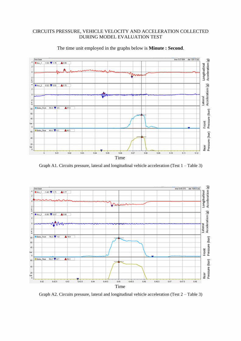
CIRCUITS PRESSURE, VEHICLE VELOCITY AND ACCELERATION COLLECTED
DURING MODEL EVALUATION TEST
The time unit employed in the graphs below is Minute : Second.
Time
Graph A1. Circuits pressure, lateral and longitudinal vehicle acceleration (Test 1 – Table 3)
Time
Graph A2. Circuits pressure, lateral and longitudinal vehicle acceleration (Test 2 – Table 3)

Time
Graph A3. Circuits pressure and longitudinal vehicle acceleration (Test 3 – Table 3)
Time
Graph A4. Circuits pressure and longitudinal vehicle acceleration (Test 4 – Table 3)

Time
Graph A5. Circuits pressure, lateral and longitudinal vehicle acceleration (Test 5 – Table 3)
Time
Graph A6. Circuits pressure and longitudinal vehicle acceleration (Test 6 – Table 3)