Brandt Lin PID

5/14/2018 Brandt Lin PID - slidepdf.com

http://slidepdf.com/reader/full/brandt-lin-pid 1/6

Proceedings of the American Control Conference

Chicago. Illinois' June 2000

Self-Tuning of PID Controllers by Adaptive Interaction. 1

Feng Lin, Robert D. Brandt, and George Saikalis

IThis research is supported in part by the National ScienceFoundation under grant ECS-9315344.FengLinis with the De-partment ofElectrical and Computer Engineering WayneStateUniversity, Detroit, MI 48202; Tel: 313-577342s, Fax: 313- We investigated the effectiveness of our self-tuning Plf)5771101,Email: fiinf@ece.eng.wayne.edu.RobertD.Brandtiscontrollersbysimulationforalargeclassofsystems.in-

with Intelligent Devic~. ~,:., 4~5Whittie: Avenue, Glen E1~yn, eluding linear and nonlinear plants stable and unstableIL 60137. George Saikahs 15 WIthHitachi, 34500 Grand River ltd I t ith d 1 'Ave., Farmington Hills, MI 48335. P an s, an p an s Wl e ays. We also simulated sys-

0-7803-5519-9/00 $10.00@2000 AACC 3676

Abstract

We propose a new self-tuning or adaptation algorithm

for PID controllers based on a theory of adaptive inter-

action. The theory develops a simple and effective way

to perform gradient descent in the parameter space.

One version of the tuning algorithm requires no knowl-

edge of the plant to be controlled. This makes the algo-

rithm robust to changes in the plant. It also makes the

algorithm universally applicable to linear and nonlinear

plants. The algorithm achieves the tuning objective by

minimizing an error function. Because of its simplicity,

the overhead for adding self-tuning is negligible. We

applied this algorithm in an automotive product man-

ufactured by Hitachi to satisfy performance require-

ments for both cold start and normal operation. Simu-lation results are presented to show the validity of the

approach.

Keywords:tuning

PID controller, adaptive control, self-

1 Introduction

Although control theory has made great advance in

t~e last few decades, which has led to many sophis-

ticated control schemes, PID control still remains the

most popular type of control being used in industries

today. This popularity is partly due to the fact that

pm controllers have simple structures and very well

understood principles. Furthermore, a well-tuned PID

controller can have excellent performance. Here, the

words "well-tuned" must be emphasized because the

performance of a Pfl) controller is crucially dependent

on the tuning process.

For the convenience of discussion, we would like to clas-

sify PID tuning into two (perhaps overlapping) classes:

(1) initial "off-line" tuning and (2) continuous "on-line"

self-tuning. Since our approach is more likely to be

used for the second class, we will focus our discussions

on this class. We believe that there are at least two rea-

sons for having an on-line self-tuning. First, the objec-

tives and hence requirements of a PID controller often

changes during the different stages of control. This is

quite evident from our experience with automotive con-

trol systems. The control objectives during the "cold

start" is often different from the "normal operation".

We believe that this is also true for many general sys-

tems. For example, we often want a system to have a

fast response time initially, but then put more emphasis

on reducing steady-state error. Fast response time and

small steady-state error are often conflicting objectives

and require different set of parameters for the PID con-

troller. Therefore, Pfl) control can be improved greatly

if we will set the para.meters initially to ensure fast re-

sponse time and then tune the parameters to reduce

steady-state error. We indeed applied this self-tuning

Pll) controller in an automotive product manufactured

by Hitachi. The result is a much improved controller.

The second reason for on-line self-tuning is that the

plant to be controlled often changes from time to time.

This is especially true if the plant is a nonlinear system

with changing operation points. When this is the case,our approach provides a simple and effective method

for adaptation of such changes.

Our approach is based on a recently developed theory of

adaptive interaction [5]-[8]. Using this theory, the con-trolled system is decomposed into four subsystems con-

sisting the plant, the proportional, integral and deriva-

tive control. The parameters of the PID control, Kp,

KJ, and KD are viewed as the interactions between

these four subsystems. A general adaptation algorithm

developed in the theory of adaptive interaction is ap-

plied to self-tuning these coefficients. The algorithm is

simple and effective.

To apply this self-tuning algorithm, the only informa-

tion needed about the plant is its Frechet derivative.For linear systems, the Frechet derivatives can be easily

calculated. Furthermore, simulation results show that

in many cases, the Frechet derivative can be replaced

by a constant that is then absorbed into the adaptation

coefficient. Using this approximated self-tuning algo-

rithm, we can eliminate any dependence on the plant

model and hence make the algorithm universal to a

large class of systems.

Another way to investigate our self-tuning algorithm

is to to view the self-tuning PID controller as a non-

linear controller because the parameters K»,KI, andKD are changing continuous according to the adapta-

tion dynamics. In general, we do not require that Kp,KI, and KD convergent to some constants. In fact

we will let them change as the inputs or disturbanceschange. Because of this property, our self-tuning pmcontrollers can do more than conventional PID con-

trollers. For example, they can stabilize systems than

cannot be stabilized by conventional PID controllers.

mailto:fiinf@ece.eng.wayne.edu.RobertD.Brandtiscontrollersbysimulationforalargeclassofsystems.in-

mailto:fiinf@ece.eng.wayne.edu.RobertD.Brandtiscontrollersbysimulationforalargeclassofsystems.in-



tems with noise and saturation. In the simulations,

weused both the Frechet self-tuning algorithm and theapproximated self-tuning algorithm. In all these simu-

lations, wehave not found any case where the closed-loop systems is unstable. Weencourage the readers to

try for themselves.

This introduction will not be completed without giv-ing referencesto other approaches to PID tuning. They

are listed at the end of the paper. To compare our ap-proache to other approaches is howevera difficult taskfor two reasons: First, there are just too many ap-

proaches to PID tuning; and secondly, our approach is

quite different from conventional approaches. There-

fore, any omission in this regard is not intentional.

This paper isorganized as follows. In Section 2, wewill

briefly present the theory of adaptive interaction that

forms the basisofour approach. In Section 3, wederive

the Frechet self-tuningalgorithm and the approximatedself-tuning algorithm. Wealsoprovethe stability oftheclosed-loopsystem with the self-tuning PID controller.

In Section 4, we present some simulation results for

various types of systems.

2 Theory of Adaptive Interaction

The theory ofadaptive interaction considers a complexsystem consisting ofN subsystems which wecalledde-

vices. Each device (indexedby n EN:= {1,2, ...,N})

has an integrable output signal Yn and an integrable in-put signal Xn. The dynamicsofeachdeviceisdescribed

by a (generally nonlinear) causal1functional

Fn: Xn _,Yn, n EN,

where Xn and Yn are the input and output spaces re-spectively. That is, the output Yn(t) of the nth device

,relates to its input xH(t) by

y,,(t) =F n o Xn )( t) =F,,[xn(t)] , n E N,

where 0 denotes composition.

We assume the Frechet derivative of Fn exists''. Wefurther assume that each deviceis a single-input single-

output system".

An interaction between twodevicesconsists ofa (gener-ally non-exclusive) functional dependence of the input

of one of the devices on the outputs of the others and

ismediated byan information carrying connections de-

noted by c. The set of all connections isdenoted by C.

1A functional . 1 " " : x . .. . .. .. y" is causal if y,,(t) depends only

on the previous history of x", {x,,(r) :r :5 t}.2the Frochet derivative 115],. 1 " : , [ " , ] , of . 1 " " [ , , , ] , is defined as a

functional such that

l' I I . ? " " [ , , , + l ! . ] - .1 "" 1 ,, , ) - . 1 " : ' [ " , ] 0l ! . 1 1 _ 0

.mll~ll--'o 1 I l ! . 1 I - .

3The assumption of single-input single-output is not as re-strictive as it may seem. This is because the partition of systeminto devices is arbitrary and up to the designer. Therefore, onecan often partition a multi-input multi-output system into sev-eral single-input single-output systems.

Weassume that there is at most one connection from

one device to another. Let pre.; be the device whose

output is conveyed by connection c and postc the de-vice whose input depends on the signal conveyed byconnection c. We denote the set of input interactions

for the nth device by I" = {c : pre ; = n} and the setof output interactions by 0" = {c : post.; = n}. Atypical system is illustrated in Figure 1. In the figure,

for example, the set of input interactions of Device 2

ish={ClJ C 3 } and the set of output interactions isO2 ={C4}' Also, Cl connects Device 1 to Device 2,

therefore preCl = 1,postcl = 2.

For the purpose of this paper, weconsider only linear

interactions, that is, we assume that the input to a

device is a linear combination of the output of otherdevices via connections in In and possibly an externalinput signal un(t):

xn(t) = n(t) +LCtcYprec(t) , n EN,eEl"

whereQe is the connection weights.

With this linear interaction, the dynamics ofthe systemis described by

Yn(t) = Fn[un(t) +LCtcYprec(t)] , n EN.eEl"

To simplify the notation, in the rest of the paper, wewill eliminate when appropriate the explicit reference

to time t.

The goal of our adaptation algorithm is to adapt theconnection weightsQe so that some performance index

E (Y l' ... , Y n, '1 1.1. ... , un) as a function of the external in-puts and outputs will be minimized. The algorithm is

given in the followingtheorem [8].

Theorem 1 For the system with dynamics given by

Yn =Fn[un +LCteYprecl, n EN,eEl"

if connection weights Cte are adapted according to

and the above equation has a unique solution, then the

performance index E will decrease monotonically withtime. In fact, the following is always satisfied

where "f > 0 is some adaptation coefficient.

The above theorem can be applied to a very generalclass of systems. For example, its application to neural

3677



networks was reported in [5]-[8].Using this algorithm,a neural network can adapt without the need of a feed-back network to back-propagate errors. The algorithm

hence provides a biologicallyplausible mechanism foradaptation in biological neurons.

Since the PID control system isspecial case of the sys-tems amendable to the aboveadaptation algorithm, the

algorithm canbesignificantlysimplifiedasshownin thenext section.

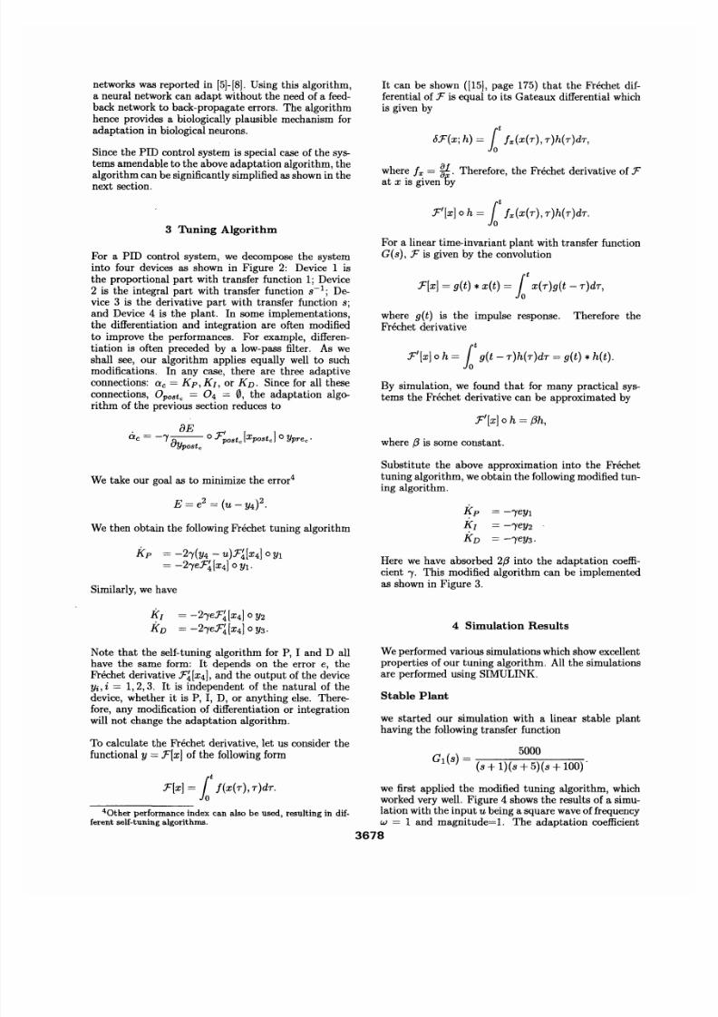
3 Tuning Algorithm

For a PID control system, wedecompose the system

into four devices as shown in Figure 2: Device 1 is

the proportional part with transfer function 1; Device

2 is the integral part with transfer function 8-1; De-

vice 3 is the derivative part with transfer function 8;

and Device 4 is the plant. In some implementations,

the differentiation and integration are often modified

to improve the performances. For example, differen-tiation is often preceded by a low-pass filter. As we

shall see, our algorithm applies equally well to suchmodifications. In any case, there are three adaptive

connections: Gc = K»,Kr, or KD. Since for all these

connections, Opostc = 04 = 0 , the adaptation algo-rithm of the previoussection reduces to

Wetake our goal as to minimize the error"

Wethen obtain the followingFreehet tuning algorithm

Kp = -2 '" )'(Y4 - U )F ~[X 4] °Yl

= - 2'" )'e F~ [x 4] 0 Yl.

Similarly, wehave

Kr = -2'")'eF~[:X4] ° Y2

KD = -21 'eF~[x41 °Y3·

Note that the self-tuning algorithm for P, I and D all

have the same form: It depends on the error e, theFrechet derivative F~[X4), and the output of the deviceYi, i= 1,2,3. It is independent of the natural of thedevice, whether it is P, I, D, or anything else. There-

fore, any modification of differentiation or integrationwill not change the adaptation algorithm.

To calculate the Frechet derivative, let us consider the

functional y =F[x ] of the followingform

F[x] = l o t I(x(T }, T )d T.

40ther performance index can also be used, resulting in dif-ferent self-tuning algorithms.

Itcan be shown ([15),page 175) that the Frechet dif-ferential ofF isequal to its Gateaux differential whichisgiven by

c5 F(x; h } = l o t t,X (T ), T }h (T }d T ,

where Ix =U ·

Therefore, the Frechet derivative ofFat x is given oy

F'[x] ° h = l o t I ",( x( T) , T )h (T )d T .

For a linear time-invariant plant with transfer function

G(8), F is given by the convolution

F[x] = g(t) * x(t) = l o t X(T )g(t - T )dT ,

where g(t) is the impulse response. Therefore the

Frechet derivative

F'[x] °h = l o tg (t - T )h(T )dT = g(t) * h(t).

By simulation, we found that for many practical sys-

tems the Frechet derivative can be approximated by

.r'[x] ° h = {3h,

where (3 is some constant.

Substitute the above approximation into the Freehettuning algorithm, weobtain the followingmodifiedtun-ing algorithm.

~P =,"),eYl

Kr =1'eY2

KD =, ") ,eY3'

Here wehave absorbed 2{3into the adaptation coeffi-

cient f.This modified algorithm can be implementedas shown in Figure 3.

4 Simulation Results

Weperformedvarioussimulations whichshowexcellent

properties ofour tuning algorithm. All the simulationsare performed usingSIMULINK.

Stable Plant

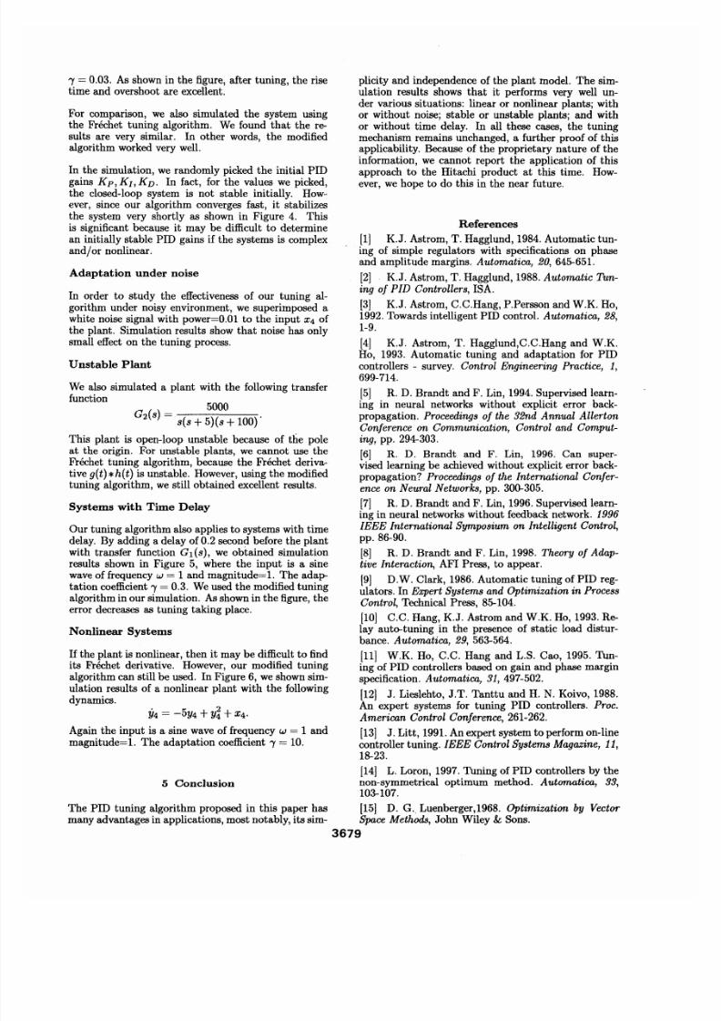
we started our simulation with a linear stable planthaving the followingtransfer function

G8- 5000

1( ) - (8+ 1)(8 + 5)(8 + 100)

we first applied the modified tuning algorithm, whichworkedverywell. Figure 4 shows the results of a simu-lationwith the input ubeinga squarewaveoffrequencyw = 1 and magnitude=l. The adaptation coefficient

3678



References

[I ] KJ. Astrom, T. Hagglund, 1984.Automatic tun-

ing of simple regulators with specifications on phase

and amplitude margins. Automatica, 20, 645-651.

[2J KJ.Astrom, T. Hagglund, 1988.Automatic Tun-ing of P ID Controllers, ISA.

[3J KJ. Astrom, C.C.Hang, P.Persson and W.K Ho,

1992.Towards intelligent PID control. Automatica, 28,

1-9.

[4J KJ. Astrom, T. Hagglund,C.C.Hang and W.K

Ho, 1993. Automatic tuning and adaptation for PIDcontrollers - survey. Control Engineering Practice, 1,699-714.

[5J R. D. Brandt and F. Lin, 1994.Supervised learn-

ing in neural networks without explicit error back-

propagation. Proceedings of the 32nd Annual AllertonConference on Communication, Control and Comput-ing, pp. 294-303.

[6] R. D. Brandt and F. Lin, 1996. Can super-

vised learning be achieved without explicit error back-

propagation? Proceedings of the International Confer-ence on Neural Networks, pp. 300-305.

[7] R. D. Brandt and F. Lin, 1996.Supervised learn-ing in neural networks without feedback network. 1996

IEEE International Symposium on Intelligent Control;pp.86-90.

[8] R. D. Brandt and F. Lin, 1998. Theory of Adap-tive Interaction, AFI Press, to appear.

[9] D.W. Clark, 1986. Automatic tuning of PID reg-

ulators. In Expert Systems and Optimization in ProcessControl, Technical Press, 85-104.

110] C.C. Hang, KJ. Astrom and W.K. Ho, 1993.Re-

lay auto-tuning in the presence of static load distur-

bance. Automatica, 29, 563-564.

[11] W.K Ho, C.C. Hang and L.S. Cao, 1995. Tun-

ing of PID controllers based on gain and phase margin

specification. Automatica, 31, 497-502.

112] J. Lieslehto, J.T. Tanttu and H. N. Koivo, 1988.

An expert systems for tuning PID controllers. Proc.

American Control Conference, 261-262.

[13J J. Litt, 1991.An expert system to perform on-linecontroller tuning. IEEE Control Systems Magazine, 11,18-23.

[14] L. Loron, 1997.Tuning of PID controllers by the

non-symmetrical optimum method. Automatica, 33,103-107.

The PID tuning algorithm proposed in this paper has [15] D. G-.Luenberger,1968. Optimization by Vectormany advantages in applications, most notably, its sirn- Space Methods, John Wiley & Sons.

3679

"y = 0.03. As shown in the figure, after tuning, the rise

time and overshoot are excellent.

For comparison, we also simulated the system using

the Frechet tuning algorithm. We found that the re-

sults are very similar. In other words, the modified

algorithm worked very well.

In the simulation, we randomly picked the initial PID

gains K»,KI, Kv. In fact, for the values we picked,

the closed-loop system is not stable initially. How-

ever, since our algorithm converges fast, it stabilizes

the system very shortly as shown in Figure 4. This

is significant because it may be difficult to determine

an initially stable PID gains if the systems is complex

and/or nonlinear.

Adaptation under noise

In order to study the effectiveness of our tuning al-

gorithm under noisy environment, we superimposed a

white noise signal with power=O.Ol to the input X4 of

the plant. Simulation results show that noise has only

small effect on the tuning process.

Unstable Plant

We also simulated a plant with the following transfer

function5000

G2(s ) = s( s + 5)(8 + 100)'

This plant is open-loop unstable because of the pole

at the origin. For unstable plants, we cannot use the

Frechet tuning algorithm, because the Frechet deriva-

tive get) *h(t) is unstable. However, using the modifiedtuning algorithm, we still obtained excellent results.

Systems with Time Delay

Our tuning algorithm also applies to systems with timedelay. By adding a delay of 0.2 second before the plant

with transfer function G1(8), we obtained simulation

results shown in Figure 5, where the input is a sinewaveof frequency w = 1and magnitudee l , The adap-

tation coefficient 'Y =0.3. Weused the modified tuning

algorithm inour simulation. Asshown in the figure, the

error decreases as tuning taking place.

Nonlinear Systems

If the plant isnonlinear, then it may be difficult to find

its Frechet derivative. However, our modified tuning

algorithm can still be used. In Figure 6, weshownsim-

ulation results of a nonlinear plant with the following

dynamics.

Again the input is a sine wave of frequency w = 1and

magnitude=L. The adaptation coefficient " Y = 10.

5 Conclusion

plicity and independence of the plant model. The sim-

ulation results shows that it performs very well un-

der various situations: linear or nonlinear plants; with

or without noise; stable or unstable plants; and with

or without time delay. In all these cases, the tuning

mechanism remains unchanged, a further proof of thisapplicability. Because of the proprietary nature of the

information, we cannot report the application of this

approach to the Hitachi product at this time. How-ever, we hope to do this in the near future.



[16] Y. Nishikawa, N. Sannomiya, T. Ohta and H.Tanaka, 1984.Amethod for auto-tuning ofPID control

parameters Automatica, 20, 321-332.

[17] Z. Shafiet and A.T. Shenton, 1994. Tuning of

PID-type controllers for stable and unstable systems

with time delay. Automatica, 30, 1609-1615.

[18] Y. Tang and R.Ortega, 1993.Adaptive tuning to

frequency response specification. Automatica, 29,1557-1563.

[19] A.A. Voda and LD. Landau, 1995. Amethod for

the auto-calibration ofPID controllers. Automatica, 31,41-53.

[20] J.G. Ziegler and N.B. Nichols, 1942.Optimal set-

ting for automatic controllers. ASME Trans., 6 4 759-768.

I D e V l c e 5 1

Figure 1: Devices and interactions

Figure 2: PID controller

Figure 3: PID Self-tuning

20.15i---r----...,-- __ -,-__ ----,

20.1

Q..

~

20.05

200 10 20 30 40

Time

1.0003

1.0002

521.0001

0.99990)-----:;1;';\0---2;;:;0:;-----=-37-_j40

Time

1.51--,- __,..--__....-_--.

-0.50)-----:;i'n-~~---='::---_j10 20 30 40

Time

4r---....---~--~__ ~

-40~-__:;';~--='::::__-_::_'_--__j10 20 30 40

Time

Figure 4: Stable plant

3680



0.8 20

0.6 15

~ 0.4 ~ 10

5

00 10 20 30 40 30 40

Time Time

0.15 4

3

0.1

~ ~2

0.051

00 0040 40

Time Time

0.09 2

0.08

1.5

0.07

~ 0.060

1~

0.050.5

0.04

0.030

0010 20 30 40 40

Time Time

3 3

2 2

(ij1

(ij1c

0) 0)

~ 0 ~ 0::I ::Ia. a.

:5-1

:5 -10 0

-2 -2

-3 -30 10 20 30 40 0 10 20 30 40

Time Time

Figure 5: System with time delay Figure 6: Nonlinear systems

3681

Documents

Brandt Lin PID