Fault size and depth extent of the Ecuador earthquake (Mw 7.8) of 16 April

2016 from teleseismic and tsunami data

Mohammad Heidarzadeh1*, Satoko Murotani2, Kenji Satake3, Tomohiro Takagawa4,

Tatsuhiko Saito5

1 Division of Civil Engineering, Department of Mechanical, Aerospace and Civil Engineering, Brunel

University London, Uxbridge, UK

2 National Museum of Nature and Science, Tsukuba, Japan

3 Earthquake Research Institute, the University of Tokyo, Tokyo, Japan

4 Port and Airport Research Institute, Yokosuka, Japan

5 National Research Institute for Earth Science and Disaster Resilience, Tsukuba, Japan

* Correspondence to:

Mohammad Heidarzadeh, Dr. Eng.,

Department of Mechanical, Aerospace and Civil Engineering,

Brunel University London,

Uxbridge, UB8 3PH

UK

Tel: +44-18952-68853

Email: mohammad.heidarzadeh@brunel.ac.uk

1

Key points:

1) The 2016 Ecuador earthquake (Mw 7.8) is similar to the 1942 event (Mw 7.8) which was

followed by 1958 (Mw 7.7) and 1979 (Mw 8.2) events.

2) While teleseismic inversion was neutral about inclusion or exclusion of slip shallower than 15

km, observed tsunamis favored the latter.

3) Final fault had a maximum slip of 2.5 m and a large-slip area of 80 km (strike-wise) × 60 km

(dip-wise) in the depth range of 15–35 km.

2

Abstract

The April 2016 Ecuador Mw 7.8 earthquake was the first megathrust tsunamigenic earthquake

along the Ecuador-Colombia subduction zone since 1979 (Mw 8.2 with 200 deaths from tsunami).

While there was no tsunami damage from the 2016 earthquake, small tsunamis were recorded at

DART and tide gauges. Here, we designed various fault models with and without shallow-slip area,

and compared the computed teleseismic and tsunami waveforms with the observations. While

teleseismic inversions were indifferent about inclusion or exclusion of the shallow slip, tsunami

waveforms strongly favored the slip model without shallow slip. Our final slip model has a depth

range of 15–44 km and its western shallowest limit is located at the distance of ~60 km from the

trench. Maximum and average slips were 2.5 and 0.7 m, respectively. The large-slip area was 80 km

(along strike) × 60 km (along dip) in the depth range of 15–35 km.

3

Introduction

A large thrust earthquake occurred on 16 April 2016 onshore Ecuador. The origin time of the

earthquake was 23:58:36 UTC with an epicenter located at 79.922oW and 0.382 oN (Figure 1)

according to the United States Geological Survey (USGS). The earthquake depth was ~21 km having

a moment magnitude (Mw) of 7.8. Based on various news reports, several nearby towns and

population centers were severely damaged resulting in a death toll of ~660 people due to the

earthquake. The resulting tsunami was small registering a maximum tide-gauge amplitude of ~10 cm

(Figure 1d). Although the tsunami did not cause any damage, the tsunami signals were clear on three

tide gauges and three Deep-ocean Assessment and Reporting of Tsunami (DART) gauges providing

valuable information to study the source of the earthquake (Figure 1d). Tsunami amplitudes were 0.5–

2 cm on DARTs.

The 2016 Ecuador earthquake was the result of the subduction of the Nazca plate beneath the

South American plate at a rate of 2.5 to 4.6 cm/yr offshore Ecuador and Colombia [Trenkamp et al.,

2002; Ye et al., 2016a,b]. The Ecuador-Colombia coast has experienced four megathrust tsunamigenic

earthquakes since 1900 AD: the events of 1906 (Mw 8.8), 1942 (Mw 7.8), 1958 (Mw 7.7), and 1979

(Mw 8.2) [Kanamori and McNally, 1982; Collot et al., 2004; Arreaga-Vargas et al., 2005] (see Figure

1c for locations and rupture zones). A northward rupture migration can be seen for the rupture zones

of the 1942, 1958 and 1979 earthquakes (Figure 1c). These previous earthquakes were tsunamigenic

and caused tsunami damage. The casualties due to the 1906 tsunami were estimated at 500–1500 by

Soloviev and Go [1979]. The 1942 and 1958 tsunamis were moderate with minimal damage and a few

deaths [Soloviev and Go, 1979]. The 1979 tsunami caused at least 200 deaths along the coast of

Colombia [Arreaga-Vargas et al., 2005].

The 2016 event is important because it is among the largest damaging earthquakes to hit the

area in decades. Furthermore, its size is similar to that of the 1942 event (both Mw 7.8) and the

aftershock distribution well covers the rupture zone of the 1942 event (Figure 1c); hence, a northward

stress transfer from this large earthquake could possibly trigger future large earthquakes to the north

of the 2016 epicenter in a way similar to the northward migrations of the 1942, 1958 and 1979

4

epicenters (Figure 1c). Although rupture patterns along subduction plate boundaries are far

unpredictable [Ando, 1975; Satake and Atwater, 2007; Stein and Okal, 2007], unilateral stress transfer

was observed in other subduction zones; e.g., southward stress transfer from the 2004 Sumatra-

Andaman Mw 9.2 earthquake [McCloskey et al., 2005] to the 2005 Nias Mw 8.7 [Kreemer et al.,

2006] and then to the 2007 Bengkulu Mw 8.4 [Fujii and Satake, 2008] megathrust tsunamigenic

earthquakes. Here, we use teleseismic and tsunami records of the 16 April 2016 event and employ

teleseismic inversions and tsunami simulations to constrain the earthquake source. We present a

source model which is consistent with both teleseismic and tsunami observations.

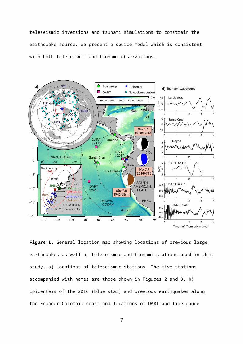
Figure 1. General location map showing locations of previous large earthquakes as well as

teleseismic and tsunami stations used in this study. a) Locations of teleseismic stations. The five

stations accompanied with names are those shown in Figures 2 and 3. b) Epicenters of the 2016 (blue

5

star) and previous earthquakes along the Ecuador-Colombia coast and locations of DART and tide

gauge stations. Dashed lines are tsunami travel time contours in hours. Focal mechanism of the 2016

event is from USGS while those of 1979 and 1942 are from Kanamori and Given [1981] and Swenson

and Beck [1996], respectively. c) Epicenters and rupture zones of previous large earthquakes based on

Kanamori and McNally [1982]. The dashed ellipses show approximations of the earthquake rupture

zones according to Kanamori and McNally [1982]. Blue solid circles show one-week aftershocks

(M>4) of the 2016 earthquake from the USGS catalog. ECU and COL stand for Ecuador and

Colombia. d) Tsunami waveforms due to the 16 April 2016 event. The first 30 min of the DART

32067 record is not available.

Data and Methods

In recent years, it has been shown that tsunami observations contain valuable information

about earthquake sources; thus, a combination of seismic and tsunami observations has been used to

obtain source models of large subduction-zone earthquakes [Satake, 1987; Yamazaki et al., 2011; Lay

et al., 2014; Inazu and Saito, 2014; Gusman et al., 2015; Li et al., 2016; Heidarzadeh et al., 2015,

2016 a,b]. We applied such a method in this study. Our data consisted of 61 teleseismic and six

tsunami records (see Figure 1 for locations). The teleseismic records were a combination of 58 P

(vertical component) in the distance range of 30–100 arc-degrees and three SH waves in the distance

range of 40–60 arc-degrees from the epicenter (Figure 1a). The three SH waves were weighted by a

factor of 0.3 while the 58 P waves were assigned a weight factor of 1.0. The tsunami data included

three DART and three tide gauge records (Figure 1d). The teleseismic records were band-pass filtered

(0.003–1.0 Hz) and the tsunami records were de-tided by estimating the tides using polynomial

fitting.

We used the program package of Kikuchi and Kanamori [2003] based on Kikuchi and

Kanamori [1991] for teleseismic body-wave inversion by setting the velocity structure according to

Laske et al. [2000] (CRUST 1.0) and Kennett et al. [1995] (ak135). We located the fault with the

strike angle of 27o, similar to the strike of the trench axis. We first assumed that fault was extended up

6

to the trench axis, and divided the fault plane into 66 subfaults (11: strike-wise × 6: dip-wise),

covering the depth range of 9.2 to 44.1 km from the sea surface (equivalent to depth 1.2–36.1 km

below seafloor). The depths reported hereafter are based on measuring from the sea surface. The

length and width of each subfault were 20 km. The depths and dip angles of the subfaults were based

on the SLAB 1.0 global subduction zone model [Hayes et al., 2012] (Figure S1 in supporting

information). As shown in the next section, we also tested limited numbers of subfaults, i.e., 55

(11×5) and 44 (11×4) subfaults on deeper parts of the plate boundary. The maximum allowed rupture

time was 20.0 s by using 9 triangles; each having duration of 4.0 s and overlapped for 2.0 s.

Maximum rupture front velocity (hereafter simply called as rupture velocity: V r) was varied in the

range 2.0–3.0 km/s with 0.25 km/s intervals in order to investigate which V r results in the best fit

between observations and computations. We note that the maximum rupture front velocity is an

assumed velocity and could be different from the physical rupture velocity which can be calculated

using snapshots of the rupture propagation. We calculated the Normalized Root Mean Square

(NRMS) misfit to quantify the match between observed and computed waveforms; for both

teleseismic body waves and tsunamis [Heidarzadeh et al., 2016a,b].

Numerical modeling of tsunami was conducted using a nonlinear shallow water model by a

finite difference method [Satake, 1995]. A single bathymetry grid having a resolution of 30 arc-sec

from the General Bathymetric Charts of the Oceans (GEBCO-2014) was used [Intergovernmental

Oceanographic Commission et al., 2014; Weatherall et al., 2015]. Time step for finite difference

computations was 1.0 s. Seafloor deformation was calculated using the dislocation model of Okada

[1985]. It is usually assumed that sea surface height, which is the initial condition for tsunami

simulation, is equivalent to seafloor deformation [Synolakis, 2003]. Therefore, we used seafloor

deformation as initial condition for tsunami simulations in this study. To examine the difference

between seafloor deformation and sea surface height, we applied a wavelength filter to the seafloor

deformation to calculate sea surface height for one of our simulations [e.g. Kajiura 1963; Saito and

Furumura 2009]. The Geoware’s [2011] software was applied for tsunami travel time analysis.

7

Results and Discussion

We first conducted inversion of teleseismic body waves for the 66 subfaults reaching the

trench axis (Figure 2), with three different assumed rupture velocities of 2.0, 2.5 and 3.0 km/s, and

simulated tsunami waveforms (Figure 2). All 61 teleseismic waveforms are shown in Figure S2 for V r

=3.0 km/s. Figure 2 shows that the large-slip area expands out of the epicenter by increasing the

rupture velocity while the maximum slip amount decreases. In terms of agreement between observed

and synthetic teleseismic waveforms, all three models give similar results (Figure 2) with NRMS

misfits of 0.485, 0.477, and 0.473 for models V r= 2.0, 2.5 and 3.0 km/s, respectively. Tsunami

simulations showed that the simulated waveforms are significantly different from model with V r=2.0

km/s (Figure 2a) to the model with V r=2.5 or 3.0 km/s (Figure 2c). The tsunami NRMS misfits were

1.055, 0.937, and 0.937 for models V r= 2.0, 2.5 and 3.0 km/s, respectively. However, an initial-early

peak is observed in tsunami simulations which does not exist in observations (arrows X2 and X3 in

Figure 2c). This initial-early peak in simulations can be attributed to the narrow co-seismic seafloor

uplift to the west of the epicenter (arrow X1 in Figure 2c). This narrow uplift is the result of shallow

slip located close to the trench axis. In fact, tsunami observations indicate that the slip area needs to

be limited to the deeper part of the plate interface.

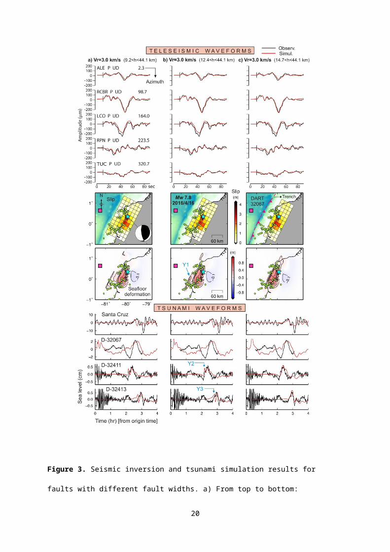
We then excluded the shallow subfaults and tested 55 (11×5) and 44 (11×4) subfault models

covering depth ranges of 12.4–44.1 km (Figure 3b) and 14.7–44.1 km (Figure 3c), respectively. The

rupture velocity is fixed at V r=3.0 km/s. Despite significant changes in fault dimensions, synthetic

teleseismic waveforms remained similar for all three cases (Figures 3 and S3). The NRMS misfits

from teleseismic inversions were 0.473 (for 11×6), 0.478 (for 11×5), and 0.489 (for 11×4) indicating

that the results were very close to each other. It can be inferred from this result that the main slip

region to explain the synthetic teleseismic waveforms exists at the deeper (> 15 km) part of the plate

interface. We also examined the down-dip limit of the fault by adding a new row of blocks to the

down-dip end of the fault plane (i.e. 77 subfaults in 11×7 grid) and performing the teleseismic

inversions for various V r. Results (Figure S4) showed that the deepest row of blocks received almost

no slip indicating that it can be removed; thus defining the down-dip limit of the fault at the depth of

8

~44 km (Figure 4 and Table S1). To study the relationship between maximum rupture front velocity

(i.e. assumed velocity) and physical rupture velocity, we plotted snapshots for various V r (Figure S5)

and realized that the assumed velocity (blue curves in Figure S5) and the physical rupture velocity

(actual snapshots in Figure S5) are almost identical.

Tsunami simulations revealed that the initial-early peak still exists for the 55-subfault model

(i.e. 11×5 in Figure 3b) while it disappeared for the 44-subfault model (i.e. 11×4 in Figure 3c). The

tsunami NRMS misfits were 0.937 (for 11×6), 0.892 (for 11×5), and 0.674 (for 11×4) indicating that

the fit between tsunami observations and simulations was significantly improved for the 44-subfault

model. By using the deep fault (i.e. 11×4; Figure 3c), it can be seen that not only the tsunami DART

records are reproduced well, but also the simulated waveform at the Santa Cruz tide gauge station was

significantly improved (i.e. the first wave was reproduced well; Figure 3c). Therefore, the deep fault

with depth range of 14.7–44.1 km is the best fault satisfying both seismic and tsunami observations

(Figure 3c). We note that the tsunami waves observed at DARTs 32411 and 32413 (located at ~1400

and ~1800 km from the epicenter) between 2 and 3 h after the origin time are different from that of

DART 32067 (located at ~160 km) around the same time interval (Figure 1d). While the former

waves are direct tsunami waves, the latter ones are from bathymetric effects; this is possibly the

reason that the DART 32067 record is not modeled well between 2 and 3 h. For the DART 32067, the

direct tsunami waves arrived within first 30 min from the origin time because this DART is located

very close to the epicenter.

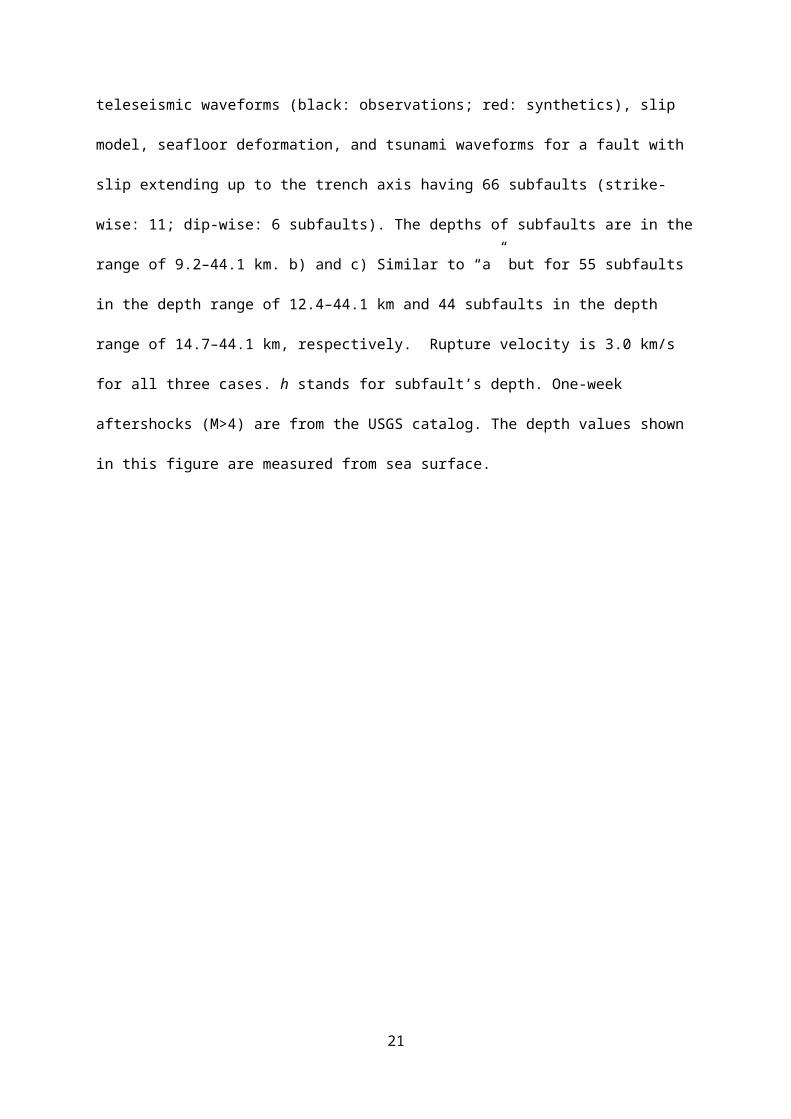
To finalize the slip model, we performed teleseismic inversion using the 44-subfault model by

changing V r from 2.0 to 3.0 km/s at 0.25 km/s intervals. The NRMS misfits for teleseismic or

tsunami results revealed that they are close to each other for different V r (Figure 4a). The minimum

NRMS misfit for teleseismic and tsunami results were obtained for models V r=3.0 km/s and V r=2.75

km/s, respectively (Figure 4a). Here, we report the model V r=3.0 km/s as the final model because

NRMS misfits are smaller for teleseismic than tsunami waveforms.

9

The final slip model is shown in Figure 4c and its details including locations of subfaults and

slip values are given in Table S1. The western shallowest limit of the slip area is located at the

distance of ~60 km from the trench axis. The fault depth is in the range of 14.7–44.1 km. Earthquake

rupture lasted for ~60 s and the maximum moment-rate occurred at ~25 s (Figure 4b). Average slip is

0.7 m (average of all non-zero slip subfaults) with a maximum slip of 2.5 m located near the

epicenter. The seismic moment is 5.32 × 1020 Nm, corresponding to Mw = 7.8. Assuming that large-

slip area is defined as subfaults with slip values larger than 1.5 times of the average slip [Murotani et

al., 2013], the large-slip area is 80 km (along strike) × 60 km (along dip) located to the south of the

epicenter (blue-dashed rectangle in Figure 4c) at a depth range of 14.7–34.7 km. Average slip on the

large-slip area is 1.7 m. The large-slip area together with the aftershock distribution confirms that the

rupture propagated southward from the epicenter. Figure 4c shows that the aftershocks are mostly

located on the borders of the large-slip area. Ye et al. [2016a] noted that aftershocks extended to the

trench axis and interpreted that shallower aftershocks were triggered by up-dip after-slip.

The source region of the 2016 earthquake is similar to that of the 1942 earthquake, which also

generated moderate tsunami damage. The 1942 event was studied by Mendoza and Dewey [1984],

Beck and Ruff [1984], Swenson and Beck [1996] and Collot et al. [2004]. The seismic moment of the

1942 event was estimated at 6–8 × 1020 Nm (equivalent to Mw 7.8–7.9) with a source-time function

showing majority of moment release within the first 24 s [Swenson and Beck, 1996]. An average slip

of ~1.2 m was reported for the 1942 event by using simple calculations based on the earthquake

moment magnitude whereas it was speculated that the local slip could be much larger [Swenson and

Beck, 1996]. Three-month aftershocks of the 1942 earthquake, from the Mendoza and Dewey [1984],

are shown in Figure S6. All the available information about the 1942 earthquake indicate that it looks

similar to the 2016 earthquake in terms of earthquake size (seismic moment), slip amounts, and

aftershock locations (Figure S6). The time interval between the 1942 and 2016 earthquakes is 74

years which corresponds to an average slip accumulation of 1.85−3.4 m by assuming a plate

convergence rate in the range of 2.5−4.6 cm/yr and given the plate coupling is high. The accumulated

slip in 74 years would be smaller if the plate coupling is low. The average slip calculated for the 2016

10

event (i.e. 1.7 m) is close to the accumulated slip for low convergence rate (i.e. ~2.5 cm/yr) with high

coupling, or high convergence rate (i.e. ~4.6 cm/yr) with low coupling, indicating that the 2016

earthquake possibly has released most of the interseismic slip accumulated at this segment of the

subduction zone. 

In this study, we assumed that initial sea surface heights are equivalent to the co-seismic

seafloor deformation. Because the slip area and seafloor deformation near trench are narrow (arrow

X1 in Figure 2c), it is important to examine whether such narrow co-seismic seafloor deformation is

equivalent to initial sea surface height or not and what are the effects on tsunami simulations. Figure

S7 shows the co-seismic seafloor deformation and initial sea surface height (by applying Kajiura

[1963] filter) for the 66-subfault model (V r=2.0 km/s). The initial sea surface height is smoother than

the co-seismic seafloor deformation. Although sharp edges existing in the co-seismic seafloor

deformation (red arrow in Figure S7) are filtered out in the initial sea surface height, the main features

remain the same for both. Especially, the small uplift near trench exists in both. Tsunami simulations

revealed that the simulated waveforms are almost the same for both (red and blue waveforms in

Figure S7).

11

Figure 2. Seismic inversion and tsunami simulation results for a fault with slip extending up to the

trench axis having 66 subfaults (strike-wise: 11; dip-wise: 6 subfaults). a) From top to bottom:

teleseismic waveforms (black: observations; red: synthetics), slip model, seafloor deformation, and

12

tsunami waveforms from the model V r=2.0 km/s. b) and c) Similar to “a” but for models V r=2.5 and

3.0 km/s, respectively. One-week aftershocks (M>4) are from the USGS catalog.

13

Figure 3. Seismic inversion and tsunami simulation results for faults with different fault widths. a)

From top to bottom: teleseismic waveforms (black: observations; red: synthetics), slip model, seafloor

deformation, and tsunami waveforms for a fault with slip extending up to the trench axis having 66

subfaults (strike-wise: 11; dip-wise: 6 subfaults). The depths of subfaults are in the range of 9.2–44.1

km. b) and c) Similar to “a” but for 55 subfaults in the depth range of 12.4–44.1 km and 44 subfaults

in the depth range of 14.7–44.1 km, respectively. Rupture velocity is 3.0 km/s for all three cases. h

stands for subfault’s depth. One-week aftershocks (M>4) are from the USGS catalog. The depth

values shown in this figure are measured from sea surface.

14

Figure 4. Final source model. a) NRMS misfits from teleseismic and tsunami simulations. b) Source-

time function for the final model with 44 subfaults whose depths are in the range of 14.7–44.1 km.

Rupture velocity is 3.0 km/s. c) Slip distribution for the final model. The dashed-blue rectangle is the

large-slip area which stands for subfaults with slip more than 1.5 times of the average slip. The depth

range of the large-slip area is 14.7–34.7 km. d) Comparison of observed and simulated waveforms for

the final source model. One-week aftershocks (M>4) are from the USGS catalog.

15

Conclusions

We studied the source of the 16 April 2016 Mw 7.8 Ecuador earthquake using teleseismic and

tsunami observations and applying teleseismic body-wave inversion and tsunami modeling. Main

findings are:

1) The 2016 Ecuador tsunami registered a maximum zero-to-peak amplitude of ~10 cm on

tide gauges and 0.5–2 cm on DART stations.

2) Teleseismic body-wave inversions using various subfault numbers, with and without

shallow slip areas (< 14.7 km), produced similar synthetic waveforms while tsunami

simulations favored a source model without shallow slip area.

3) The final slip model lacks the slip in shallow region, with the depth range of 14.7–44.1

km, and the western border of the fault plane is located at the distance of ~60 km from the

trench axis. The maximum and average slip values are 2.5 and 0.7 m, respectively. The

large-slip area is 80 km (along strike) × 60 km (along dip) located to the south of the

epicenter indicating southward propagation of the earthquake rupture. Average slip on the

large-slip area, in the depth range of 14.7–34.7 km, is 1.7 m.

Acknowledgements

We downloaded tide gauge data from the Intergovernmental Oceanographic Commission’s

website (http://www.ioc-sealevelmonitoring.org/). DART data were also downloaded from the

website of NOAA on 16 April 2016 (http://nctr.pmel.noaa.gov/Dart/). We downloaded teleseismic

records of the earthquakes from Incorporated Research Institutions for Seismology website at:

http://www.iris.edu/wilber3/find_event. We used the teleseismic body-wave inversion program from

http://wwweic.eri.u-tokyo.ac.jp/ETAL/KIKUCHI/. Earthquake focal mechanism data of

Global Centroid-Moment-Tensor Project (GCMT) were used in this study

(http://www.globalcmt.org/). All figures were drafted by using the GMT software [Wessel and Smith,

16

1998]. We are grateful to Dr. Andrew Newman (editor), Dr. Thorne Lay (University of California

Santa Cruz), and an anonymous reviewer for constructive review comments.

17

References

Ando, M. (1975), Source mechanism and tectonic significance of historical earthquakes along the

Nankai trough, Japan, Tectonophys. 27, 119–140.

Angermann, D., J. Klotz, and C. Reigber (1999), Space-geodetic estimation of the Nazca-South

America Euler vector, Earth Planet. Sci. Lett., 171(3), 329-334.

Beck, S.L. and L.J. Ruff (1984), The rupture process of the great 1979 Colombia earthquake:

Evidence for the asperity model, J. Geophys. Res., 89(B11), 9281-9291.

Collot, J.-Y., B. Marcaillou, F. Sage, F. Michaud, W. Agudelo, Ph. Charvis, D. Graindorge, M.- A.

Gutscher, and G. Spence (2004), Are rupture zone limits of great subduction earthquakes

controlled by upper plate structures? Evidence from multichannel seismic reflection data

acquired across the northern Ecuador–southwest Colombia margin, J. Geophys. Res.: Solid

Earth109, doi:10.1029/2004JB003060.

Fujii, Y. and K. Satake (2008), Tsunami waveform inversion of the 2007 Bengkulu, southern

Sumatra, earthquake, Earth planets space, 60(9), 993-998.

Geoware (2011), The tsunami travel times (TTT), Available at:

http://www.geoware-online.com/tsunami.html.

Gusman, A.R., S. Murotani, K. Satake, M. Heidarzadeh, E. Gunawan, S. Watada, and B. Schurr,

(2015), Fault slip distribution of the 2014 Iquique, Chile, earthquake estimated from ocean-wide

tsunami waveforms and GPS data, Geophys. Res. Lett., 42(4), 1053-1060.

Hayes, G.P., D. J. Wald, and R.L. Johnson (2012), Slab1. 0: A three-dimensional model of global

subduction zone geometries, J. Geophys. Res., 117(B1), 10.1029/2011JB008524.

Heidarzadeh, M., A. R. Gusman, T. Harada, and K. Satake (2015), Tsunamis from the 29 March and 5

May 2015 Papua New Guinea earthquake doublet (Mw 7.5) and tsunamigenic potential of the

New Britain trench, Geophys. Res. Lett., 42, 5958–5965.

18

Heidarzadeh, M., S. Murotani, K. Satake, T. Ishibe, and A.R. Gusman, (2016a), Source model of the

16 September 2015 Illapel, Chile Mw 8.4 earthquake based on teleseismic and tsunami

data, Geophys. Res. Lett., 43, doi: 10.1002/2015GL067297.

Heidarzadeh, M., T. Harada, K. Satake, T. Ishibe, and A.R. Gusman (2016b), Comparative study of

two tsunamigenic earthquakes in the Solomon Islands: 2015 Mw 7.0 normal-fault and 2013

Santa Cruz Mw 8.0 megathrust earthquakes, Geophys. Res. Lett., 43(9), 4340-4349

Heidarzadeh, M., and K. Satake, (2014), Excitation of basin-wide modes of the Pacific Ocean

following the March 2011 Tohoku tsunami, Pure Appl. Geophys., 171(12), 3405-3419.

Inazu, D. and T. Saito (2014), Two subevents across the Japan Trench during the 7 December 2012

off Tohoku earthquake (Mw 7.3) inferred from offshore tsunami records, J. Geophys. Res.: Solid

Earth,119(7), 5800-5813

Intergovernmental Oceanographic Commission et al. (2014), Centenary Edition of the GEBCO

Digital Atlas, published on CD-ROM on behalf of the Intergovernmental Oceanographic

Commission and the International Hydrographic Organization as part of the General Bathymetric

Chart of the Oceans, British Oceanographic Data Centre, Liverpool, U.K.

Kajiura, K. (1963), The leading wave of a tsunami, Bull. Earthquake Res. Inst., 41, 535–571.

Kanamori, H. and J.W. Given (1981), Use of long-period surface waves for rapid determination of

earthquake-source parameters, Phys. Earth Planet. Int., 27(1), 8-31.

Kanamori, H., and K. C. McNally (1982), Variable rupture mode of the subduction zone along the

Ecuador-Colombia coast, Bull. Seismol. Soc. Am. 72(4), 1241-1253.

Kennett, B. L. N., E. R. Engdahl, and R. Buland (1995), Constraints on seismic velocities in the Earth

from travel times, Geophys. J. Int., 122, 108–124.

Kikuchi, M., and H., Kanamori (1991), Inversion of complex body waves – III, Bull. Seismolo. Soc.

Am., 81(6), 2335-2350.

19

Kikuchi M., and H. Kanamori (2003), Note on Teleseismic Body-Wave Inversion Program,

http://www.eri.u-tokyo.ac.jp/ETAL/KIKUCHI/.

Kreemer, C., G. Blewitt, and F. Maerten (2006), Co-and postseismic deformation of the 28 March

2005 Nias Mw 8.7 earthquake from continuous GPS data, Geophys. Res. Lett., 33(7),

doi: 10.1029/2005GL025566.

Laske, G., G. Masters., Z. Ma, and M. Pasyanos (2013), Update on CRUST1.0 - A 1-degree Global

Model of Earth's Crust, Geophys. Res. Abstracts, 15, Abstract EGU2013-2658.

Lay, T., H. Yue, E.E. Brodsky, and C. An, (2014), The 1 April 2014 Iquique, Chile, Mw 8.1

earthquake rupture sequence, Geophys. Res. Lett., 41(11), 3818-3825.

Li, L., T. Lay, K.F. Cheung, and L.Ye (2016), Joint modeling of teleseismic and tsunami wave

observations to constrain the 16 September 2015 Illapel, Chile, Mw 8.3 earthquake rupture

process, Geophys. Res. Lett., 43(9), 4303-4312.

Mendoza, C. and J.W. Dewey (1984), Seismicity associated with the great Colombia-Ecuador

earthquakes of 1942, 1958, and 1979: Implications for barrier models of earthquake rupture,

Bull. Seismol. Soc. Am., 74(2), 577-593.

McCloskey, J., S.S. Nalbant, and S. Steacy (2005), Indonesian earthquake: Earthquake risk from co-

seismic stress, Nature, 434(7031), 291-291.

Murotani, S., K. Satake, and Y. Fujii (2013), Scaling relations of seismic moment, rupture area,

average slip, and asperity size for M ~ 9 subduction-zone earthquakes, Geophys. Res. Lett., 40,

5070–5074.

Okada, Y. (1985), Surface deformation due to shear and tensile faults in a half-space, Bull. Seismolo.

Soc. Am., 75, 1135-1154.

Saito, T., and T. Furumura (2009), Three-dimensional tsunami generation simulation due to sea-

bottom deformation and its interpretation based on the linear theory, Geophys. J. Int., 178, 877–

888.

20

Satake, K. (1987), Inversion of tsunami waveforms for the estimation of a fault heterogeneity: Method

and numerical experiments, J. Phys. Earth, 35(3), 241-254.

Satake, K. (1995), Linear and nonlinear computations of the 1992 Nicaragua earthquake tsunami,

Pure Appl. Geophys., 144, 455-470.

Satake K., B. Atwater (2007), Long-term perspectives on giant earthquakes and tsunamis at

subduction zones, Annu Rev Earth Planet Sci, 35, 349-74.

Swenson, J.L. and S.L. Beck (1996), Historical 1942 Ecuador and 1942 Peru subduction earthquakes

and earthquake cycles along Colombia-Ecuador and Peru subduction segments, Pure Appl.

Geophys., 146(1), 67-101.

Soloviev, L., and N. Go (1975), A catalogue of tsunamis on the eastern shore of the Pacific Ocean

(1513-1968), Nauka Publishing House, Moscow, USSR, 204p.

Stein, S., and E.A. Okal (2007), Ultra-long period seismic study of the December 2004 Indian Ocean

earthquake and implications for regional tectonics and the subduction process, Bull. Seismol.

Soc. Am., 97, S279-S295. 

Synolakis, C.E. (2003), Tsunami and seiche. In: Chen, W.F., Scawthorn, C. (Eds.), Earthquake

Engineering Handbook. CRC Press. Chapter 9, pp. 1–90.

Trenkamp, R., J.N. Kellogg, J.T. Freymueller and H.P. Mora (2002), Wide plate margin deformation,

southern Central America and northwestern South America, CASA GPS observations, J. South

Ame. Earth Sci., 15(2), 157-171.

Wessel, P., and W. H. F., Smith (1998), New, Improved Version of Generic Mapping Tools

Released, EOS Trans., AGU, 79 (47), 579.

Weatherall, P., K. M. Marks, M. Jakobsson, T. Schmitt, S. Tani, J. E. Arndt, M. Rovere, D. Chayes,

V. Ferrini, and R. Wigley (2015), A new digital bathymetric model of the world's oceans, Earth

and Space Science, 2, 331–345, doi:10.1002/2015EA000107.

21

Yamazaki, Y., T. Lay, K.F. Cheung, H. Yue, and H. Kanamori (2011), Modeling near‐field tsunami

observations to improve finite‐fault slip models for the 11 March 2011 Tohoku

earthquake, Geophys. Res. Lett., 38(7), doi: 10.1029/2011GL049130.

Ye, L., H. Kanamori, J.P. Avouac, L. Li, K.F. Cheung, and T. Lay (2016a), The 16 April 2016, M W

7.8 (M S 7.5) Ecuador earthquake: A quasi-repeat of the 1942 M S 7.5 earthquake and partial re-

rupture of the 1906 M S 8.6 Colombia–Ecuador earthquake, Earth Planet. Sci. Lett., 454, 248-

258.

Ye, L., H. Kanamori, J.P. Avouac, L. Li, K.F. Cheung, and T. Lay (2016b), Corrigendum to “The 16

April 2016, M W 7.8 (M S 7.5) Ecuador earthquake: A quasi-repeat of the 1942 M S 7.5

earthquake and partial re-rupture of the 1906 M S 8.6 Colombia–Ecuador earthquake”, Earth

Planet. Sci. Lett., 454, 248-258.

22