Embed Size (px)
Citation preview

Business Intelligence Trends商業智慧趨勢
1
1012BIT05MIS MBA
Mon 6, 7 (13:10-15:00) Q407
商業智慧的資料探勘 (Data Mining for
Business Intelligence)
Min-Yuh Day戴敏育
Assistant Professor專任助理教授
Dept. of Information Management, Tamkang University淡江大學 資訊管理學系
http://mail. tku.edu.tw/myday/2013-03-18
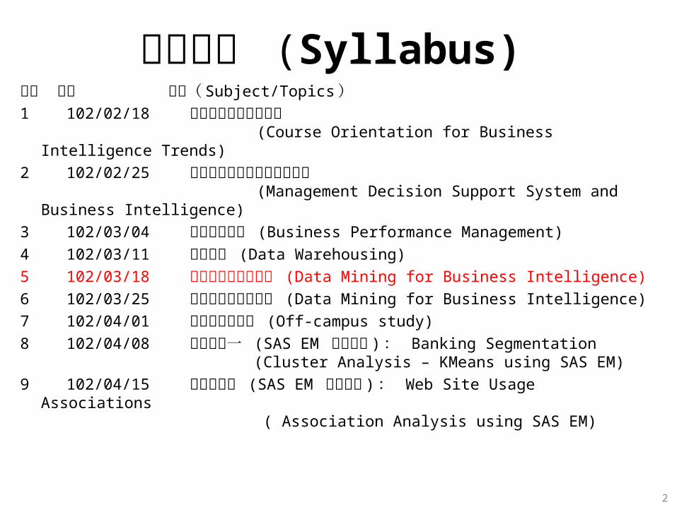
週次 日期 內容( Subject/Topics )1 102/02/18 商業智慧趨勢課程介紹
(Course Orientation for Business Intelligence Trends)
2 102/02/25 管理決策支援系統與商業智慧 (Management Decision Support System and Business Intelligence)
3 102/03/04 企業績效管理 (Business Performance Management)4 102/03/11 資料倉儲 (Data Warehousing)5 102/03/18 商業智慧的資料探勘 (Data Mining for Business Intelligence)6 102/03/25 商業智慧的資料探勘 (Data Mining for Business Intelligence)7 102/04/01 教學行政觀摩日 (Off-campus study)8 102/04/08 個案分析一 (SAS EM 分群分析 ) : Banking Segmentation
(Cluster Analysis – KMeans using SAS EM)9 102/04/15 個案分析二 (SAS EM 關連分析 ) : Web Site Usage Associations
( Association Analysis using SAS EM)
課程大綱 (Syllabus)
2
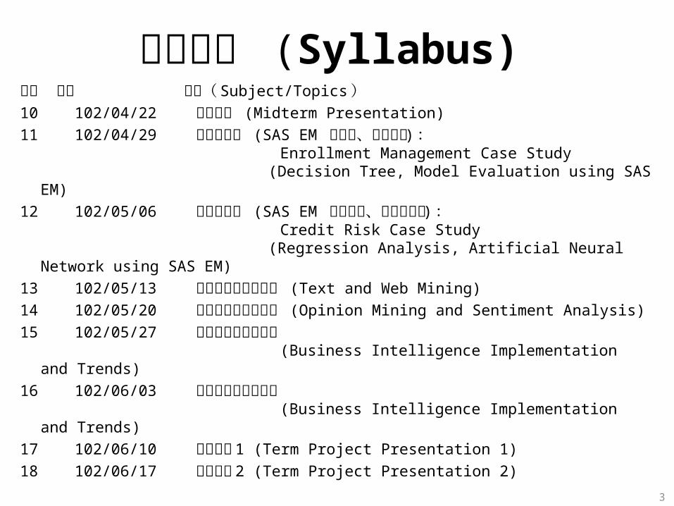
週次 日期 內容( Subject/Topics )10 102/04/22 期中報告 (Midterm Presentation)11 102/04/29 個案分析三 (SAS EM 決策樹、模型評估 ) :
Enrollment Management Case Study (Decision Tree, Model Evaluation using SAS EM)
12 102/05/06 個案分析四 (SAS EM 迴歸分析、類神經網路 ) : Credit Risk Case Study (Regression Analysis, Artificial Neural Network using SAS EM)
13 102/05/13 文字探勘與網路探勘 (Text and Web Mining)14 102/05/20 意見探勘與情感分析 (Opinion Mining and Sentiment Analysis)15 102/05/27 商業智慧導入與趨勢
(Business Intelligence Implementation and Trends)
16 102/06/03 商業智慧導入與趨勢 (Business Intelligence Implementation and Trends)
17 102/06/10 期末報告 1 (Term Project Presentation 1)18 102/06/17 期末報告 2 (Term Project Presentation 2)
課程大綱 (Syllabus)
3
Decision Support and Business Intelligence Systems
(9th Ed., Prentice Hall)
Chapter 5:Data Mining for
Business Intelligence
Source: Turban et al. (2011), Decision Support and Business Intelligence Systems 4

Learning Objectives• Define data mining as an enabling technology for
business intelligence• Standardized data mining processes
– CRISP-DM– SEMMA
• Association Analysis– Association Rule Mining (Apriori Algorithm)
• Classification– Decision Tree
• Cluster Analysis– K-Means Clustering
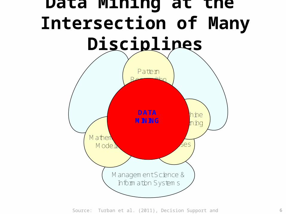
Data Mining at the Intersection of Many Disciplines
Management Science & Information Systems
Databases
Pattern Recognition
MachineLearning
MathematicalModeling
DATAMINING
Source: Turban et al. (2011), Decision Support and Business Intelligence Systems 6
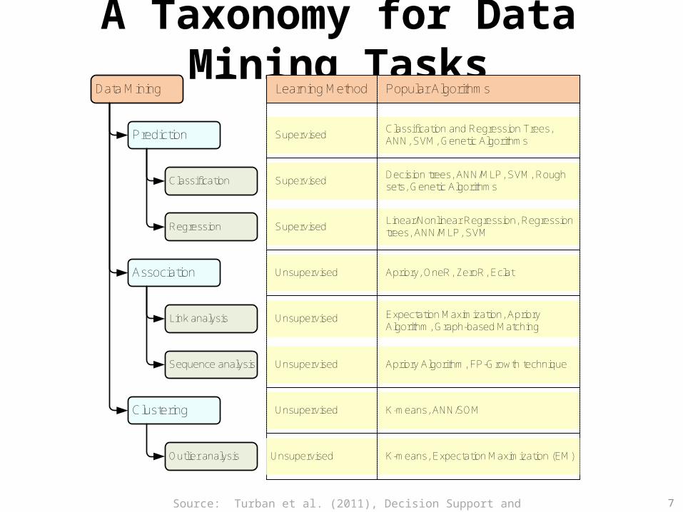
A Taxonomy for Data Mining TasksData Mining
Prediction
Classification
Regression
Clustering
Association
Link analysis
Sequence analysis
Learning Method Popular Algorithms
Supervised
Supervised
Supervised
Unsupervised
Unsupervised
Unsupervised
Unsupervised
Decision trees, ANN/MLP, SVM, Rough sets, Genetic Algorithms
Linear/Nonlinear Regression, Regression trees, ANN/MLP, SVM
Expectation Maximization, Apriory Algorithm, Graph-based Matching
Apriory Algorithm, FP-Growth technique
K-means, ANN/SOM
Outlier analysis Unsupervised K-means, Expectation Maximization (EM)
Apriory, OneR, ZeroR, Eclat
Classification and Regression Trees, ANN, SVM, Genetic Algorithms
Source: Turban et al. (2011), Decision Support and Business Intelligence Systems 7
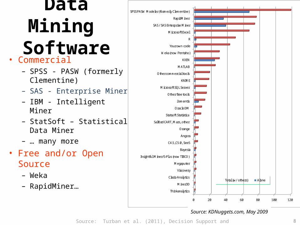
Data Mining Software
• Commercial – SPSS - PASW (formerly
Clementine)– SAS - Enterprise Miner– IBM - Intelligent Miner– StatSoft – Statistical Data
Miner– … many more
• Free and/or Open Source– Weka– RapidMiner…
0 20 40 60 80 100 120
Thinkanalytics
Miner3D
Clario Analytics
Viscovery
Megaputer
Insightful Miner/S-Plus (now TIBCO)
Bayesia
C4.5, C5.0, See5
Angoss
Orange
Salford CART, Mars, other
Statsoft Statistica
Oracle DM
Zementis
Other free tools
Microsoft SQL Server
KNIME
Other commercial tools
MATLAB
KXEN
Weka (now Pentaho)
Your own code
R
Microsoft Excel
SAS / SAS Enterprise Miner
RapidMiner
SPSS PASW Modeler (formerly Clementine)
Total (w/ others) Alone
Source: KDNuggets.com, May 2009
Source: Turban et al. (2011), Decision Support and Business Intelligence Systems 8

Why Data Mining?• More intense competition at the global scale • Recognition of the value in data sources• Availability of quality data on customers, vendors,
transactions, Web, etc. • Consolidation and integration of data repositories into
data warehouses• The exponential increase in data processing and
storage capabilities; and decrease in cost• Movement toward conversion of information
resources into nonphysical form
Source: Turban et al. (2011), Decision Support and Business Intelligence Systems 9
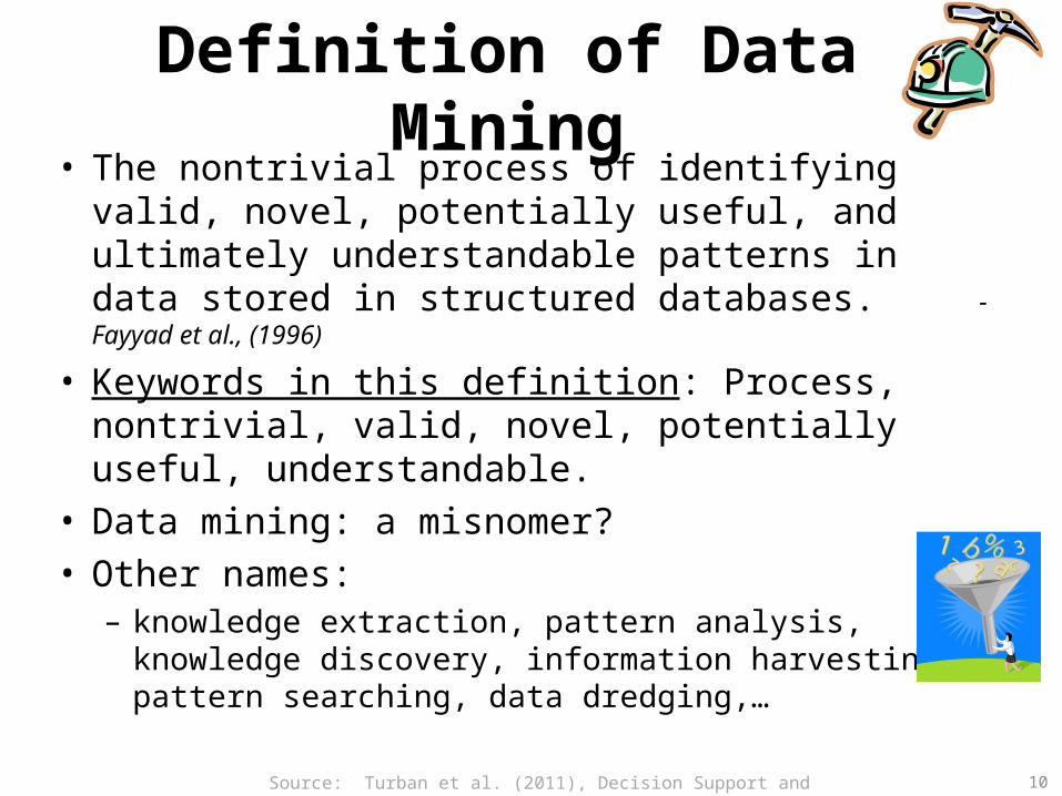
Definition of Data Mining• The nontrivial process of identifying valid, novel,
potentially useful, and ultimately understandable patterns in data stored in structured databases. - Fayyad et al., (1996)
• Keywords in this definition: Process, nontrivial, valid, novel, potentially useful, understandable.
• Data mining: a misnomer?• Other names:
– knowledge extraction, pattern analysis, knowledge discovery, information harvesting, pattern searching, data dredging,…
Source: Turban et al. (2011), Decision Support and Business Intelligence Systems 10
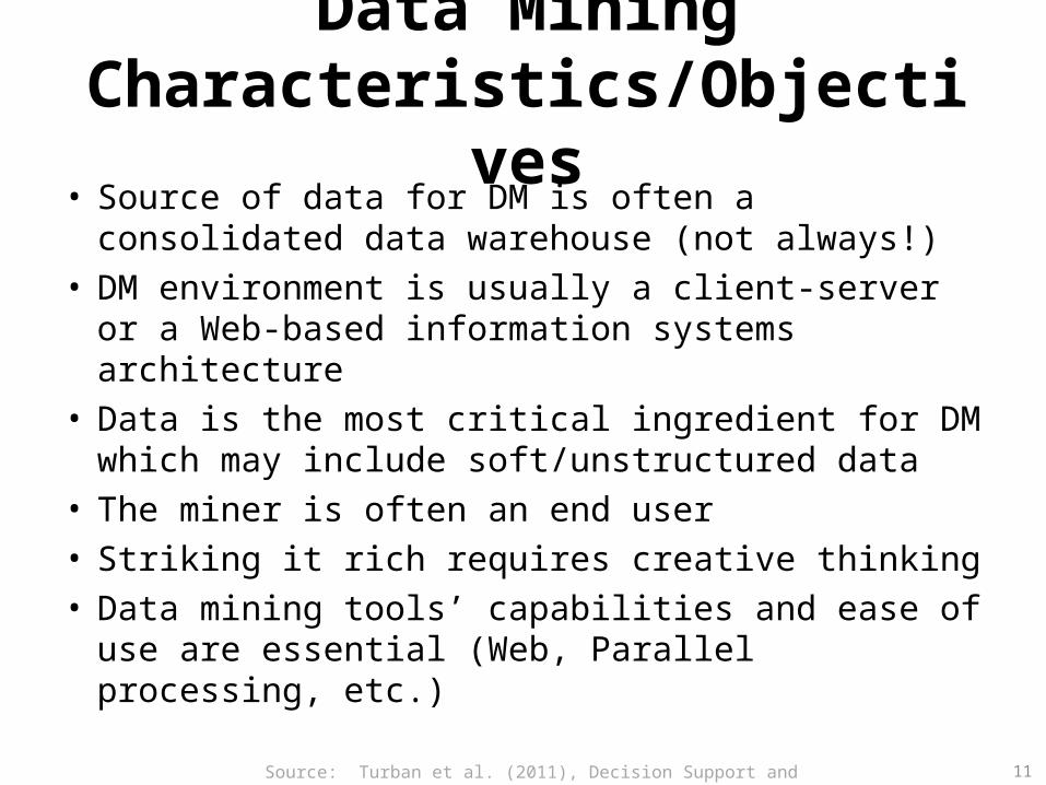
Data Mining Characteristics/Objectives
• Source of data for DM is often a consolidated data warehouse (not always!)
• DM environment is usually a client-server or a Web-based information systems architecture
• Data is the most critical ingredient for DM which may include soft/unstructured data
• The miner is often an end user• Striking it rich requires creative thinking• Data mining tools’ capabilities and ease of use are
essential (Web, Parallel processing, etc.)
Source: Turban et al. (2011), Decision Support and Business Intelligence Systems 11

Data in Data Mining
Data
Categorical Numerical
Nominal Ordinal Interval Ratio
• Data: a collection of facts usually obtained as the result of experiences, observations, or experiments
• Data may consist of numbers, words, images, …• Data: lowest level of abstraction (from which information and
knowledge are derived)
- DM with different data types?
- Other data types?
Source: Turban et al. (2011), Decision Support and Business Intelligence Systems 12
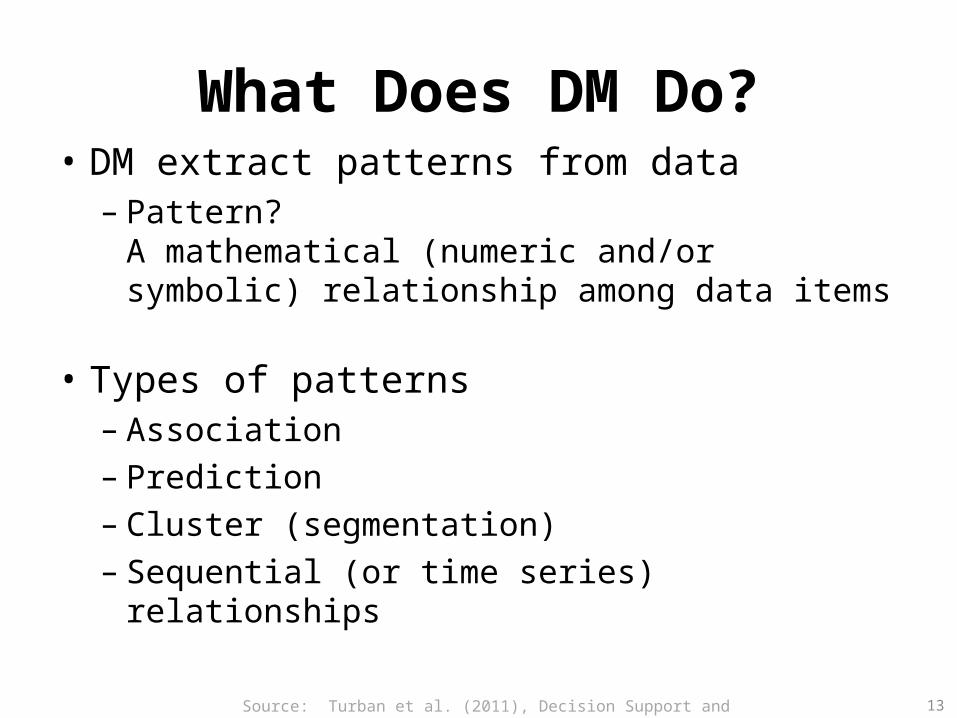
What Does DM Do?• DM extract patterns from data
– Pattern? A mathematical (numeric and/or symbolic) relationship among data items
• Types of patterns– Association– Prediction– Cluster (segmentation)– Sequential (or time series) relationships
Source: Turban et al. (2011), Decision Support and Business Intelligence Systems 13
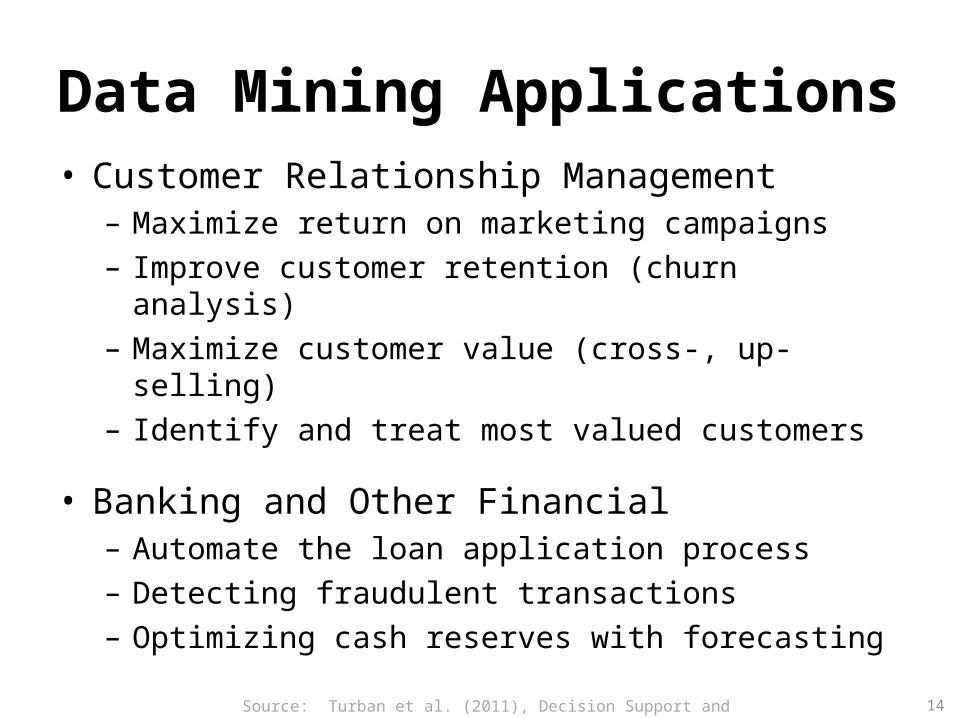
Data Mining Applications• Customer Relationship Management
– Maximize return on marketing campaigns– Improve customer retention (churn analysis)– Maximize customer value (cross-, up-selling)– Identify and treat most valued customers
• Banking and Other Financial – Automate the loan application process – Detecting fraudulent transactions– Optimizing cash reserves with forecasting
Source: Turban et al. (2011), Decision Support and Business Intelligence Systems 14
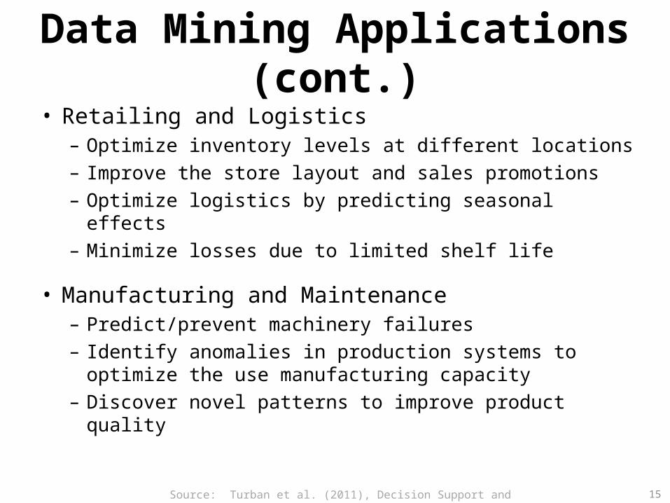
Data Mining Applications (cont.)• Retailing and Logistics
– Optimize inventory levels at different locations– Improve the store layout and sales promotions– Optimize logistics by predicting seasonal effects– Minimize losses due to limited shelf life
• Manufacturing and Maintenance– Predict/prevent machinery failures – Identify anomalies in production systems to optimize the
use manufacturing capacity– Discover novel patterns to improve product quality
Source: Turban et al. (2011), Decision Support and Business Intelligence Systems 15
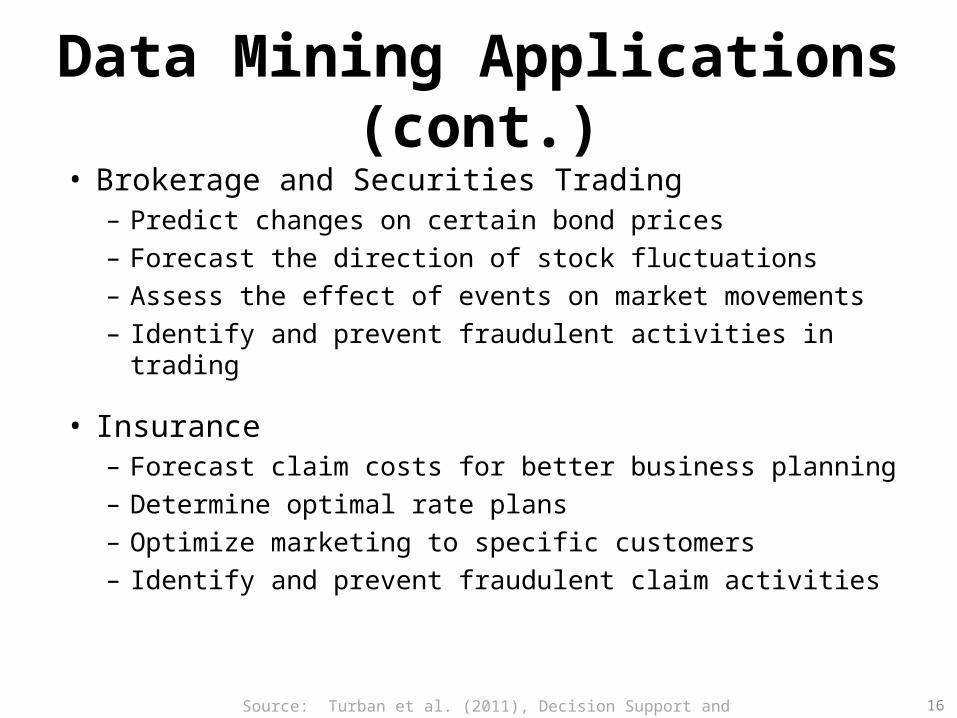
Data Mining Applications (cont.)• Brokerage and Securities Trading
– Predict changes on certain bond prices – Forecast the direction of stock fluctuations– Assess the effect of events on market movements– Identify and prevent fraudulent activities in trading
• Insurance– Forecast claim costs for better business planning– Determine optimal rate plans – Optimize marketing to specific customers – Identify and prevent fraudulent claim activities
Source: Turban et al. (2011), Decision Support and Business Intelligence Systems 16
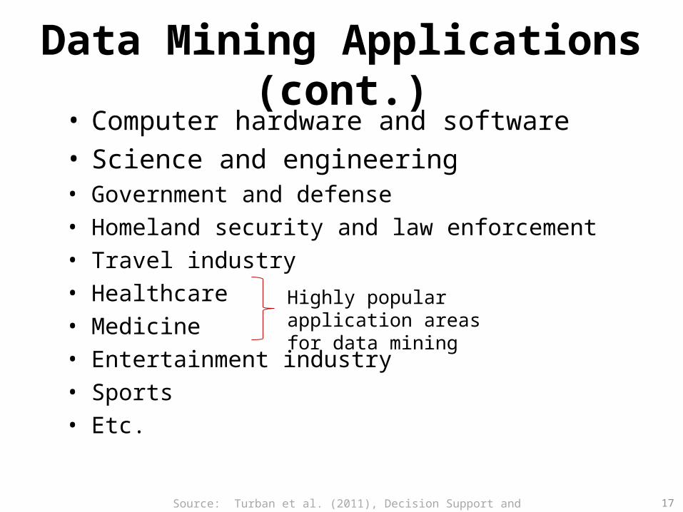
Data Mining Applications (cont.)• Computer hardware and software• Science and engineering• Government and defense• Homeland security and law enforcement• Travel industry • Healthcare• Medicine• Entertainment industry• Sports• Etc.
Highly popular application areas for data mining
Source: Turban et al. (2011), Decision Support and Business Intelligence Systems 17
Data Mining Process• A manifestation of best practices• A systematic way to conduct DM projects• Different groups has different versions• Most common standard processes:
– CRISP-DM (Cross-Industry Standard Process for Data Mining)
– SEMMA (Sample, Explore, Modify, Model, and Assess)
– KDD (Knowledge Discovery in Databases)
Source: Turban et al. (2011), Decision Support and Business Intelligence Systems 18
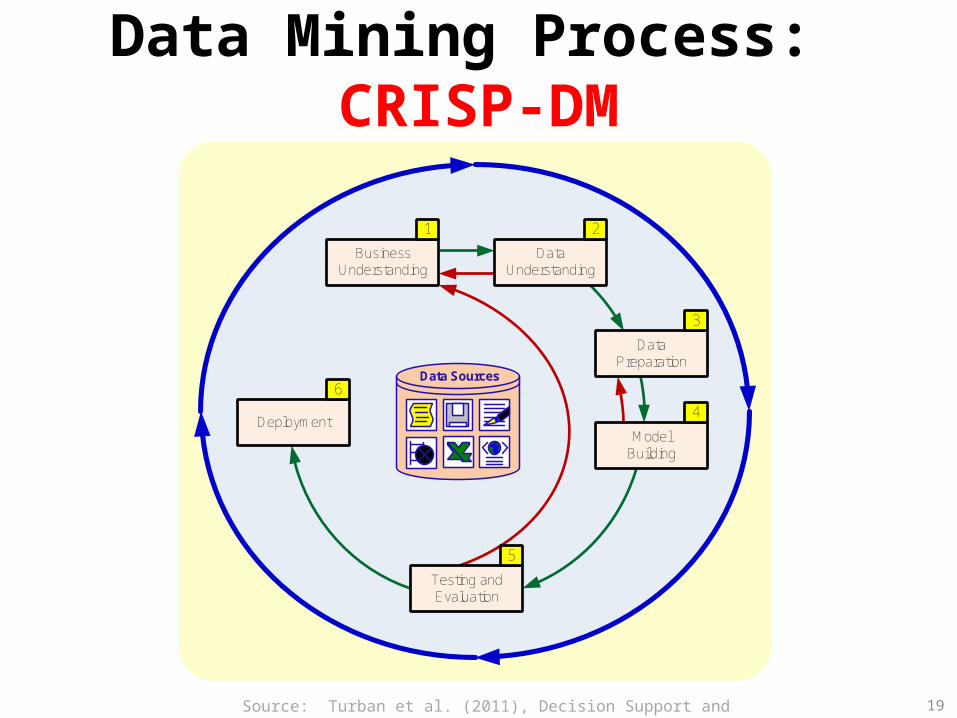
Data Mining Process: CRISP-DM
Data Sources
Business Understanding
Data Preparation
Model Building
Testing and Evaluation
Deployment
Data Understanding
6
1 2
3
5
4
Source: Turban et al. (2011), Decision Support and Business Intelligence Systems 19
Data Mining Process: CRISP-DM
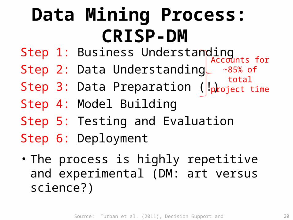
Step 1: Business UnderstandingStep 2: Data UnderstandingStep 3: Data Preparation (!)Step 4: Model BuildingStep 5: Testing and EvaluationStep 6: Deployment
• The process is highly repetitive and experimental (DM: art versus science?)
Accounts for ~85% of total project time
Source: Turban et al. (2011), Decision Support and Business Intelligence Systems 20

Data Preparation – A Critical DM Task
Data Consolidation
Data Cleaning
Data Transformation
Data Reduction
Well-formedData
Real-worldData
· Collect data· Select data· Integrate data
· Impute missing values· Reduce noise in data · Eliminate inconsistencies
· Normalize data· Discretize/aggregate data · Construct new attributes
· Reduce number of variables· Reduce number of cases · Balance skewed data
Source: Turban et al. (2011), Decision Support and Business Intelligence Systems 21

Data Mining Process: SEMMA
Sample
(Generate a representative sample of the data)
Modify(Select variables, transform
variable representations)
Explore(Visualization and basic description of the data)
Model(Use variety of statistical and machine learning models )
Assess(Evaluate the accuracy and usefulness of the models)
SEMMA
Source: Turban et al. (2011), Decision Support and Business Intelligence Systems 22
Data Mining Methods: Classification
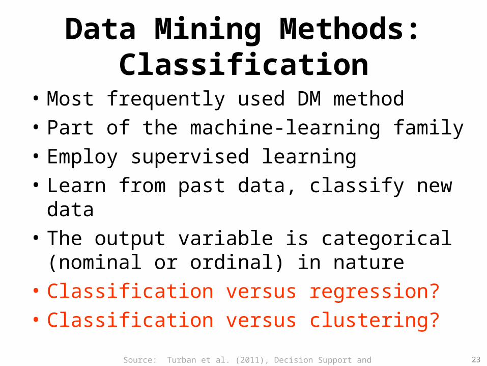
• Most frequently used DM method• Part of the machine-learning family • Employ supervised learning• Learn from past data, classify new data• The output variable is categorical
(nominal or ordinal) in nature• Classification versus regression?• Classification versus clustering?
Source: Turban et al. (2011), Decision Support and Business Intelligence Systems 23
Assessment Methods for Classification
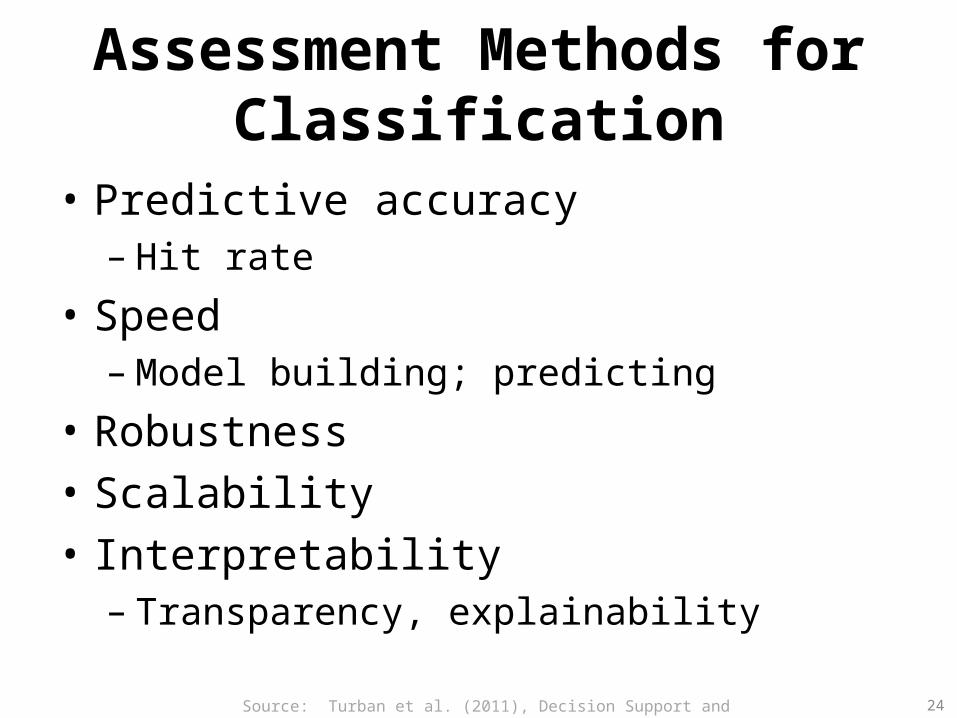
• Predictive accuracy– Hit rate
• Speed– Model building; predicting
• Robustness• Scalability• Interpretability
– Transparency, explainability
Source: Turban et al. (2011), Decision Support and Business Intelligence Systems 24

Accuracy
Precision
25
Validity
Reliability

26
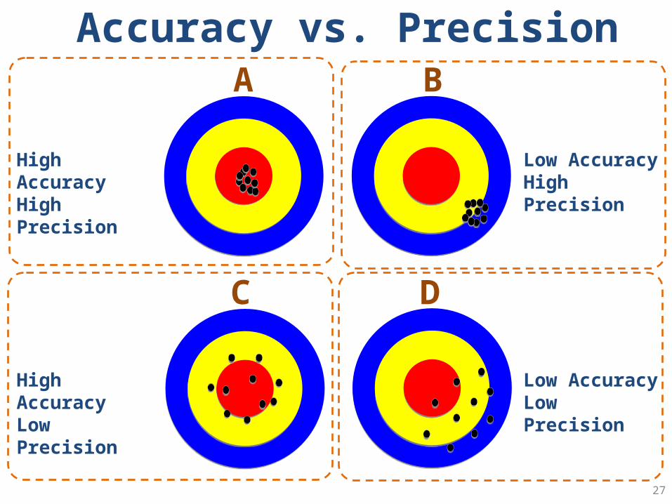
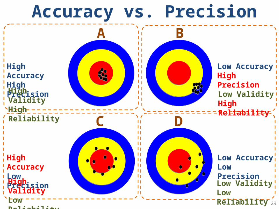
Accuracy vs. Precision
27
High AccuracyHigh Precision
High AccuracyLow Precision
Low AccuracyHigh Precision
Low AccuracyLow Precision
A B
C D

Accuracy vs. Precision
28
High AccuracyHigh Precision
High AccuracyLow Precision
Low AccuracyHigh Precision
Low AccuracyLow Precision
A B
C D
High ValidityHigh Reliability
High ValidityLow Reliability
Low ValidityLow Reliability
Low ValidityHigh Reliability
Accuracy vs. Precision
29
High AccuracyHigh Precision
High AccuracyLow Precision
Low AccuracyHigh Precision
Low AccuracyLow Precision
A B
C D
High ValidityHigh Reliability
High ValidityLow Reliability
Low ValidityLow Reliability
Low ValidityHigh Reliability
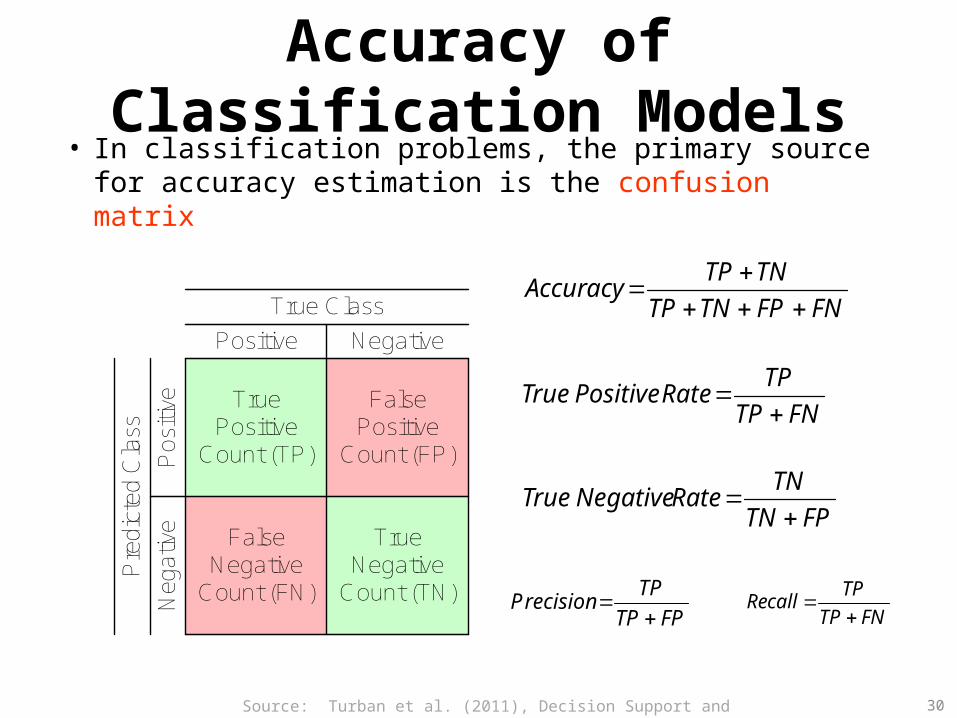
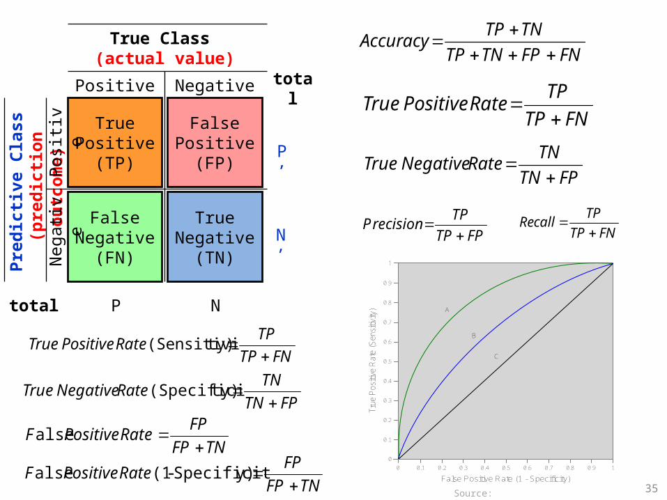
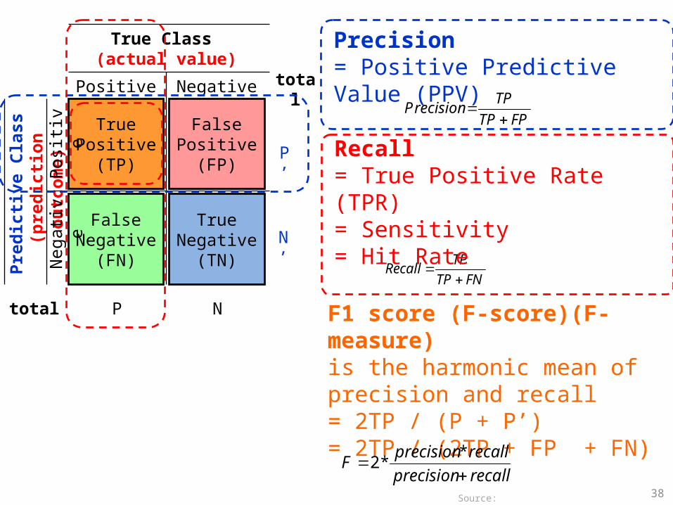
Accuracy of Classification Models• In classification problems, the primary source for
accuracy estimation is the confusion matrix
True Positive
Count (TP)
FalsePositive
Count (FP)
TrueNegative
Count (TN)
FalseNegative
Count (FN)
True Class
Positive Negative
Pos
itive
Neg
ativ
e
Pre
dict
ed C
lass
FNTP
TPRatePositiveTrue
FPTN
TNRateNegativeTrue
FNFPTNTP
TNTPAccuracy
FPTP
TPrecision
P
FNTP
TPcallRe
Source: Turban et al. (2011), Decision Support and Business Intelligence Systems 30

Estimation Methodologies for Classification
• Simple split (or holdout or test sample estimation) – Split the data into 2 mutually exclusive sets
training (~70%) and testing (30%)
– For ANN, the data is split into three sub-sets (training [~60%], validation [~20%], testing [~20%])
PreprocessedData
Training Data
Testing Data
Model Development
Model Assessment
(scoring)
2/3
1/3
Classifier
Prediction Accuracy
Source: Turban et al. (2011), Decision Support and Business Intelligence Systems 31
Estimation Methodologies for Classification
• k-Fold Cross Validation (rotation estimation) – Split the data into k mutually exclusive subsets– Use each subset as testing while using the rest of the
subsets as training– Repeat the experimentation for k times – Aggregate the test results for true estimation of prediction
accuracy training
• Other estimation methodologies– Leave-one-out, bootstrapping, jackknifing– Area under the ROC curve
Source: Turban et al. (2011), Decision Support and Business Intelligence Systems 32
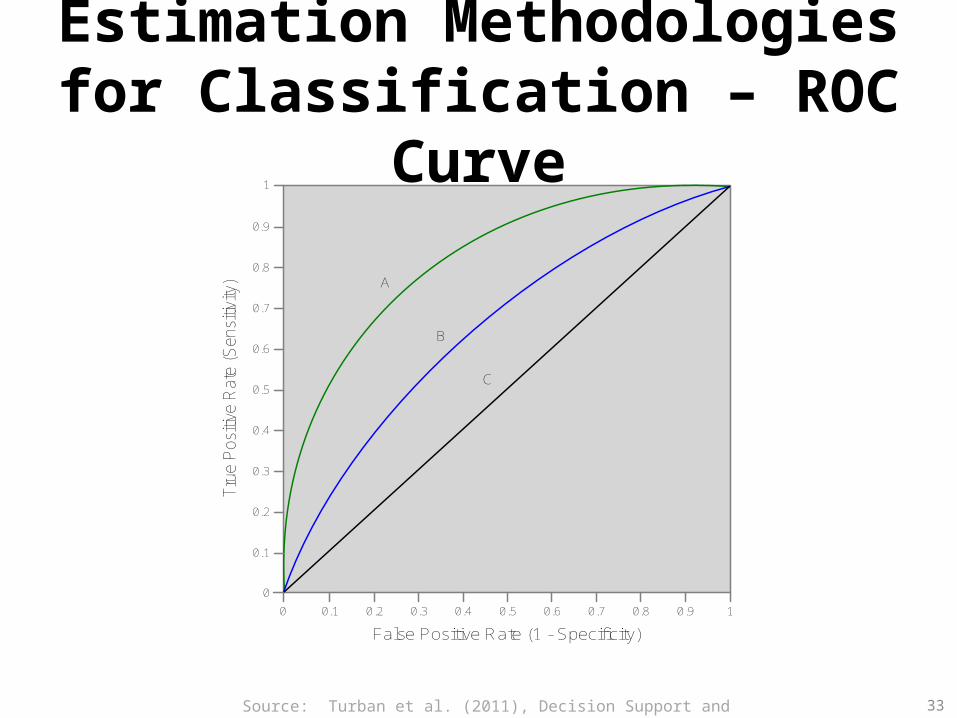
Estimation Methodologies for Classification – ROC Curve
10.90.80.70.60.50.40.30.20.10
0
0.1
0.2
0.3
0.4
0.5
0.6
0.7
1
0.9
0.8
False Positive Rate (1 - Specificity)
Tru
e P
ositi
ve R
ate
(Sen
sitiv
ity) A
B
C
Source: Turban et al. (2011), Decision Support and Business Intelligence Systems 33
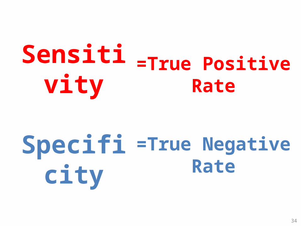
Sensitivity
Specificity
34
=True Positive Rate
=True Negative Rate
TruePositive
(TP)
FalseNegative
(FN)
FalsePositive
(FP)
TrueNegative
(TN)
True Class (actual value)
Pre
dic
tive
Cla
ss
(pre
dic
tio
n o
utc
om
e)P
ositi
veN
egat
ive
Positive Negative
total P
total
N
N’
P’
35
FNTP
TPRatePositiveTrue
FPTN
TNRateNegativeTrue
FNFPTNTP
TNTPAccuracy
FPTP
TPrecision
P
FNTP
TPcallRe
FNTP
TPRatePositiveTrue
ty)(Sensitivi
10.90.80.70.60.50.40.30.20.10
0
0.1
0.2
0.3
0.4
0.5
0.6
0.7
1
0.9
0.8
False Positive Rate (1 - Specificity)
True
Pos
itive
Rat
e (S
ensi
tivity
) A
B
C
TNFP
FPRatePositiveF
alse
FPTN
TNRateNegativeTrue
ty)(Specifici
TNFP
FPRatePositiveF
y)Specificit-(1 alse
Source: http://en.wikipedia.org/wiki/Receiver_operating_characteristic
TruePositive
(TP)
FalseNegative
(FN)
FalsePositive
(FP)
TrueNegative
(TN)
True Class (actual value)
Pre
dic
tive
Cla
ss
(pre
dic
tio
n o
utc
om
e)P
ositi
veN
egat
ive
Positive Negative
total P
total
N
N’
P’
36
FNTP
TPRatePositiveTrue
FNTP
TPcallRe
FNTP
TPRatePositiveTrue
ty)(Sensitivi
10.90.80.70.60.50.40.30.20.10
0
0.1
0.2
0.3
0.4
0.5
0.6
0.7
1
0.9
0.8
False Positive Rate (1 - Specificity)
True
Pos
itive
Rat
e (S
ensi
tivity
) A
B
C
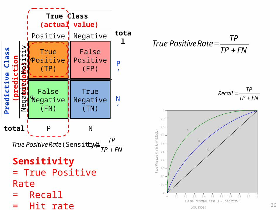
Sensitivity= True Positive Rate = Recall = Hit rate= TP / (TP + FN) Source: http://en.wikipedia.org/wiki/Receiver_operating_characteristic
TruePositive
(TP)
FalseNegative
(FN)
FalsePositive
(FP)
TrueNegative
(TN)
True Class (actual value)
Pre
dic
tive
Cla
ss
(pre
dic
tio
n o
utc
om
e)P
ositi
veN
egat
ive
Positive Negative
total P
total
N
N’
P’
37
FPTN
TNRateNegativeTrue
10.90.80.70.60.50.40.30.20.10
0
0.1
0.2
0.3
0.4
0.5
0.6
0.7
1
0.9
0.8
False Positive Rate (1 - Specificity)
True
Pos
itive
Rat
e (S
ensi
tivity
) A
B
C
FPTN
TNRateNegativeTrue
ty)(Specifici
TNFP
FPRatePositiveF
y)Specificit-(1 alse
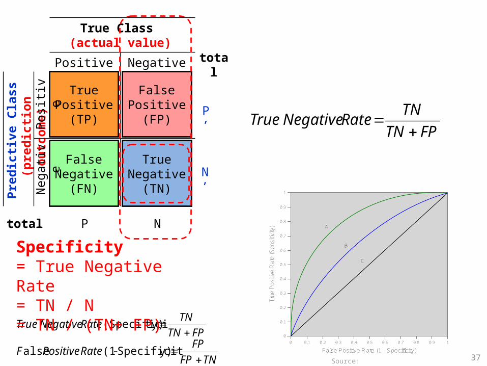
Specificity= True Negative Rate= TN / N= TN / (TN+ FP)
Source: http://en.wikipedia.org/wiki/Receiver_operating_characteristic
TruePositive
(TP)
FalseNegative
(FN)
FalsePositive
(FP)
TrueNegative
(TN)
True Class (actual value)
Pre
dic
tive
Cla
ss
(pre
dic
tio
n o
utc
om
e)P
ositi
veN
egat
ive
Positive Negative
total P
total
N
N’
P’
38
FPTP
TPrecision
P
FNTP
TPcallRe
F1 score (F-score)(F-measure)is the harmonic mean of precision and recall= 2TP / (P + P’)= 2TP / (2TP + FP + FN)
Precision = Positive Predictive Value (PPV)
Recall = True Positive Rate (TPR)= Sensitivity = Hit Rate
recallprecision
recallprecisionF
**2
Source: http://en.wikipedia.org/wiki/Receiver_operating_characteristic
39Source: http://en.wikipedia.org/wiki/Receiver_operating_characteristic
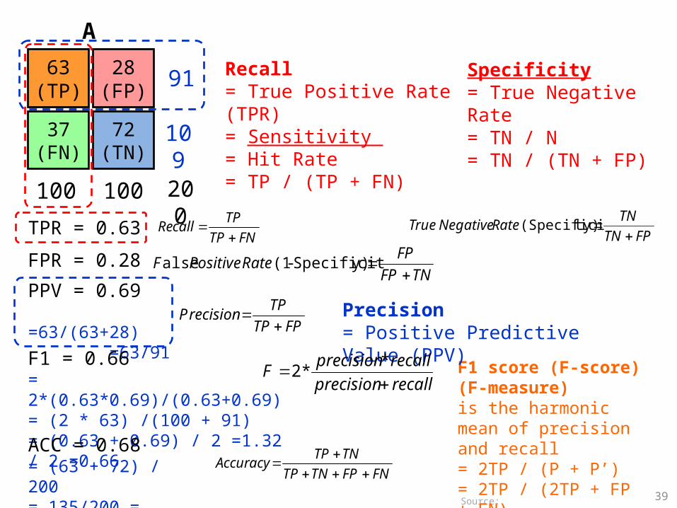
A
63(TP)
37(FN)
28(FP)
72(TN)
100 100
109
91
200
TPR = 0.63
FPR = 0.28
PPV = 0.69 =63/(63+28) =63/91
F1 = 0.66 = 2*(0.63*0.69)/(0.63+0.69)= (2 * 63) /(100 + 91)= (0.63 + 0.69) / 2 =1.32 / 2 =0.66
ACC = 0.68= (63 + 72) / 200= 135/200 = 67.5
FPTP
TPrecision
P
FNTP
TPcallRe
F1 score (F-score)(F-measure)is the harmonic mean of precision and recall= 2TP / (P + P’)= 2TP / (2TP + FP + FN)
Precision = Positive Predictive Value (PPV)
Recall = True Positive Rate (TPR)= Sensitivity = Hit Rate= TP / (TP + FN)
recallprecision
recallprecisionF
**2
FNFPTNTP
TNTPAccuracy
FPTN
TNRateNegativeTrue
ty)(Specifici
TNFP
FPRatePositiveF
y)Specificit-(1 alse
Specificity= True Negative Rate= TN / N= TN / (TN + FP)

40Source: http://en.wikipedia.org/wiki/Receiver_operating_characteristic
A
63(TP)
37(FN)
28(FP)
72(TN)
100 100
109
91
200
TPR = 0.63
FPR = 0.28
PPV = 0.69 =63/(63+28) =63/91
F1 = 0.66 = 2*(0.63*0.69)/(0.63+0.69)= (2 * 63) /(100 + 91)= (0.63 + 0.69) / 2 =1.32 / 2 =0.66
ACC = 0.68= (63 + 72) / 200= 135/200 = 67.5
B
77(TP)
23(FN)
77(FP)
23(TN)
100 100
46
154
200
TPR = 0.77FPR = 0.77PPV = 0.50F1 = 0.61ACC = 0.50
FNTP
TPcallRe
Recall = True Positive Rate (TPR)= Sensitivity = Hit Rate
Precision = Positive Predictive Value (PPV) FPTP
TPrecision
P

41
C’
76(TP)
24(FN)
12(FP)
88(TN)
100 100
112
88
200
TPR = 0.76FPR = 0.12PPV = 0.86F1 = 0.81ACC = 0.82
C
24(TP)
76(FN)
88(FP)
12(TN)
100 100
88
112
200
TPR = 0.24FPR = 0.88PPV = 0.21F1 = 0.22ACC = 0.18
Source: http://en.wikipedia.org/wiki/Receiver_operating_characteristic
FNTP
TPcallRe
Recall = True Positive Rate (TPR)= Sensitivity = Hit Rate
Precision = Positive Predictive Value (PPV) FPTP
TPrecision
P

42
Market Basket Analysis
Source: Han & Kamber (2006)
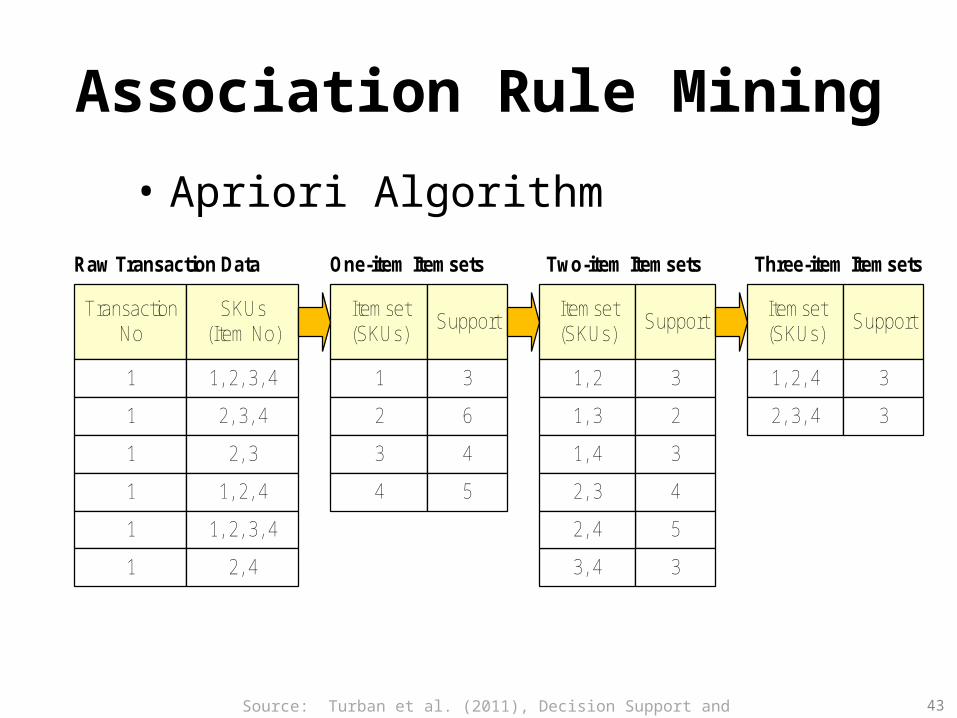
Association Rule Mining
• Apriori Algorithm
Itemset(SKUs)
SupportTransaction
NoSKUs
(Item No)
1
1
1
1
1
1
1, 2, 3, 4
2, 3, 4
2, 3
1, 2, 4
1, 2, 3, 4
2, 4
Raw Transaction Data
1
2
3
4
3
6
4
5
Itemset(SKUs)
Support
1, 2
1, 3
1, 4
2, 3
3
2
3
4
3, 4
5
3
2, 4
Itemset(SKUs)
Support
1, 2, 4
2, 3, 4
3
3
One-item Itemsets Two-item Itemsets Three-item Itemsets
Source: Turban et al. (2011), Decision Support and Business Intelligence Systems 43

Association Rule Mining• A very popular DM method in business• Finds interesting relationships (affinities) between
variables (items or events)• Part of machine learning family• Employs unsupervised learning• There is no output variable• Also known as market basket analysis• Often used as an example to describe DM to
ordinary people, such as the famous “relationship between diapers and beers!”
Source: Turban et al. (2011), Decision Support and Business Intelligence Systems 44
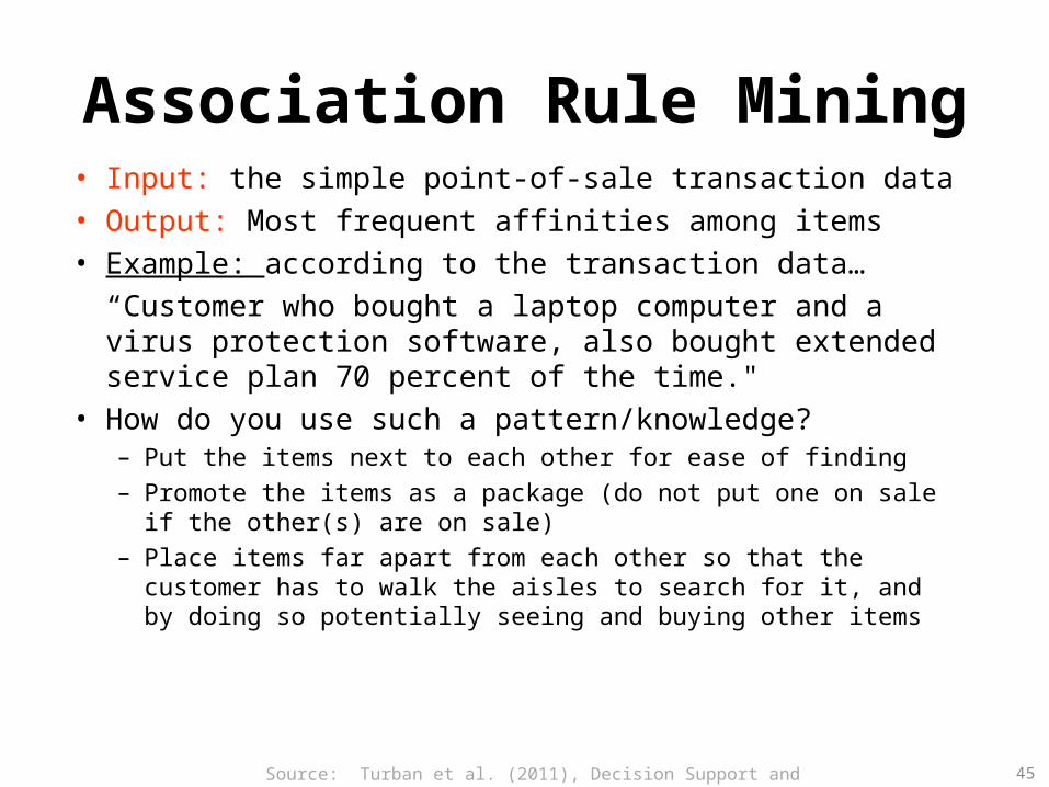
Association Rule Mining• Input: the simple point-of-sale transaction data• Output: Most frequent affinities among items • Example: according to the transaction data…
“Customer who bought a laptop computer and a virus protection software, also bought extended service plan 70 percent of the time."
• How do you use such a pattern/knowledge?– Put the items next to each other for ease of finding– Promote the items as a package (do not put one on sale if the
other(s) are on sale) – Place items far apart from each other so that the customer has to
walk the aisles to search for it, and by doing so potentially seeing and buying other items
Source: Turban et al. (2011), Decision Support and Business Intelligence Systems 45
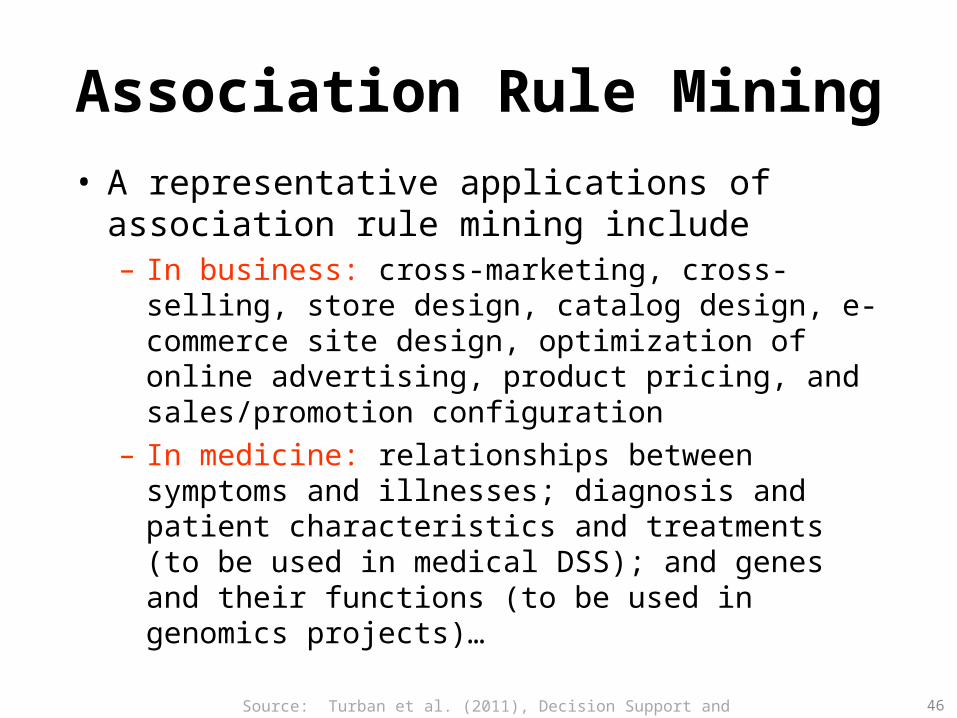
Association Rule Mining• A representative applications of association rule
mining include– In business: cross-marketing, cross-selling, store design,
catalog design, e-commerce site design, optimization of online advertising, product pricing, and sales/promotion configuration
– In medicine: relationships between symptoms and illnesses; diagnosis and patient characteristics and treatments (to be used in medical DSS); and genes and their functions (to be used in genomics projects)…
Source: Turban et al. (2011), Decision Support and Business Intelligence Systems 46
Association Rule Mining
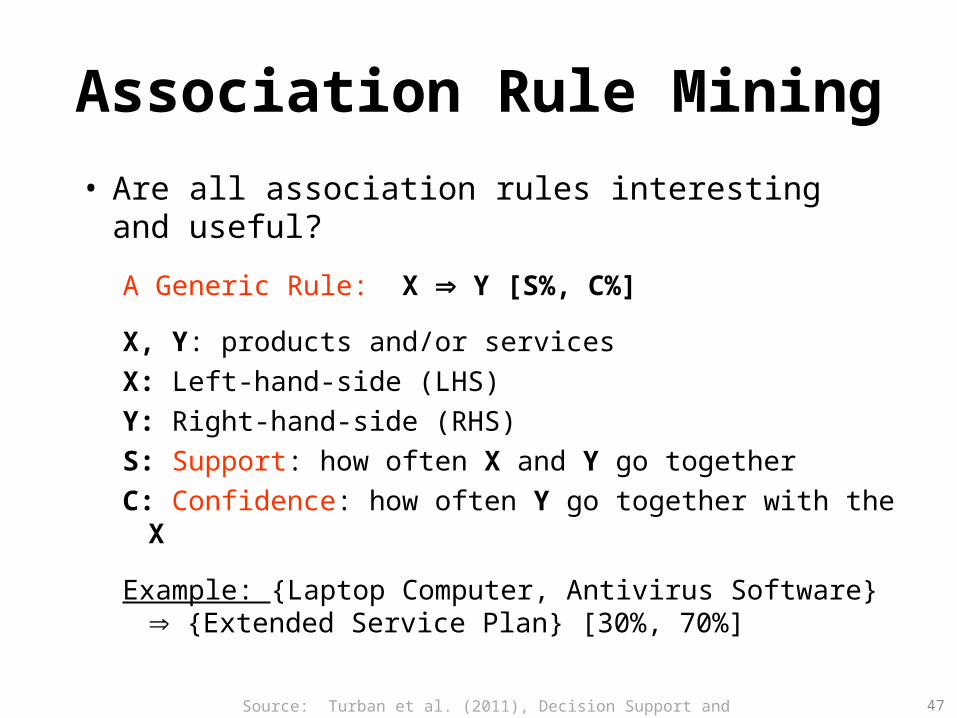
• Are all association rules interesting and useful?
A Generic Rule: X Y [S%, C%]
X, Y: products and/or services X: Left-hand-side (LHS)Y: Right-hand-side (RHS)S: Support: how often X and Y go togetherC: Confidence: how often Y go together with the X
Example: {Laptop Computer, Antivirus Software} {Extended Service Plan} [30%, 70%]
Source: Turban et al. (2011), Decision Support and Business Intelligence Systems 47
Association Rule Mining
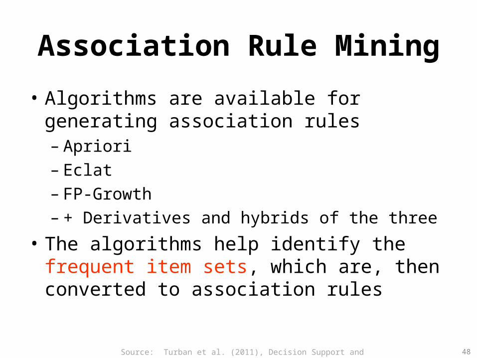
• Algorithms are available for generating association rules– Apriori– Eclat– FP-Growth– + Derivatives and hybrids of the three
• The algorithms help identify the frequent item sets, which are, then converted to association rules
Source: Turban et al. (2011), Decision Support and Business Intelligence Systems 48
Association Rule Mining
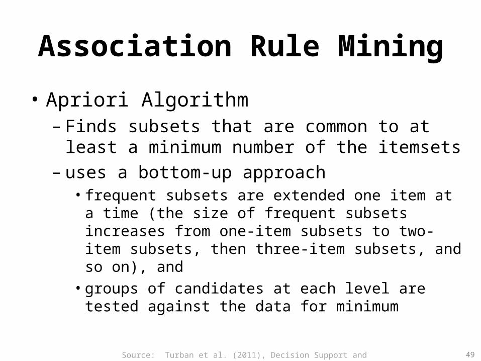
• Apriori Algorithm– Finds subsets that are common to at least a
minimum number of the itemsets– uses a bottom-up approach
• frequent subsets are extended one item at a time (the size of frequent subsets increases from one-item subsets to two-item subsets, then three-item subsets, and so on), and
• groups of candidates at each level are tested against the data for minimum
Source: Turban et al. (2011), Decision Support and Business Intelligence Systems 49
50
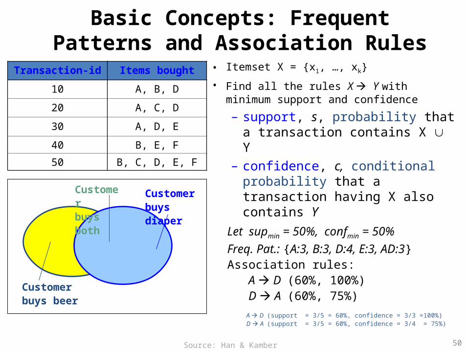
Basic Concepts: Frequent Patterns and Association Rules
• Itemset X = {x1, …, xk}
• Find all the rules X Y with minimum support and confidence
– support, s, probability that a transaction contains X Y
– confidence, c, conditional probability that a transaction having X also contains Y
Let supmin = 50%, confmin = 50%
Freq. Pat.: {A:3, B:3, D:4, E:3, AD:3}Association rules:
A D (60%, 100%)D A (60%, 75%)
Customerbuys diaper
Customerbuys both
Customerbuys beer
Transaction-id Items bought
10 A, B, D
20 A, C, D
30 A, D, E
40 B, E, F
50 B, C, D, E, F
A D (support = 3/5 = 60%, confidence = 3/3 =100%)D A (support = 3/5 = 60%, confidence = 3/4 = 75%)
Source: Han & Kamber (2006)

Market basket analysis• Example
– Which groups or sets of items are customers likely to purchase on a given trip to the store?
• Association Rule– Computer antivirus_software
[support = 2%; confidence = 60%]• A support of 2% means that 2% of all the transactions
under analysis show that computer and antivirus software are purchased together.
• A confidence of 60% means that 60% of the customers who purchased a computer also bought the software.
51Source: Han & Kamber (2006)
Association rules
• Association rules are considered interesting if they satisfy both – a minimum support threshold and – a minimum confidence threshold.
52Source: Han & Kamber (2006)
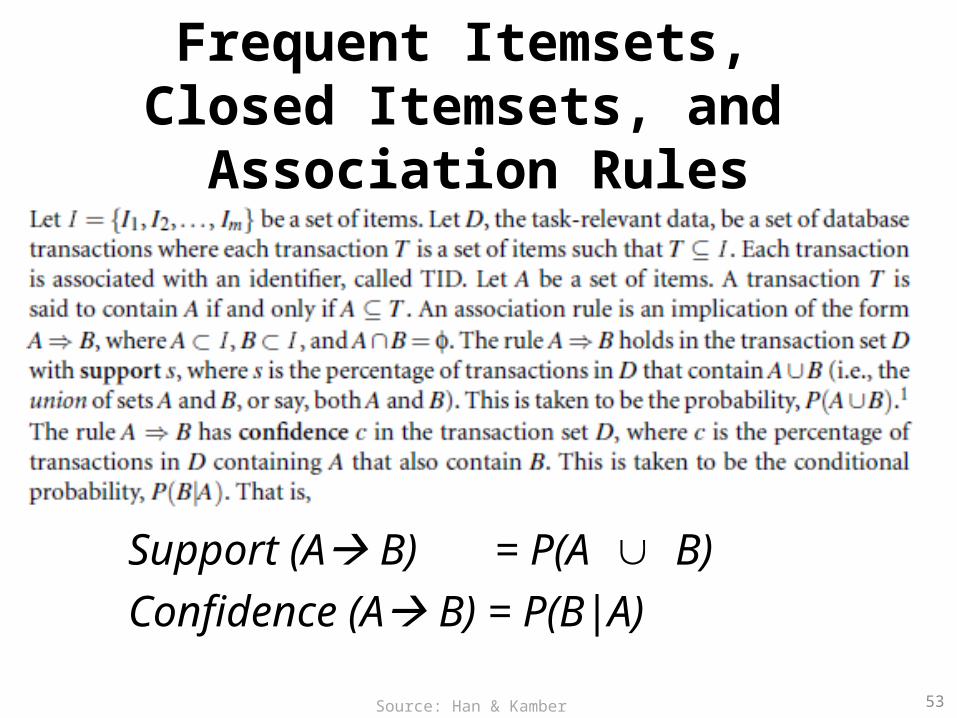
Frequent Itemsets, Closed Itemsets, and
Association Rules
53
Support (A B) = P(A B)Confidence (A B) = P(B|A)
Source: Han & Kamber (2006)
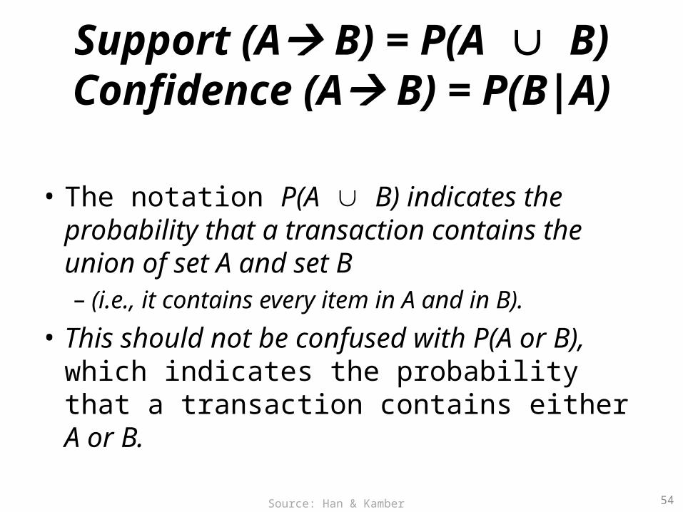
Support (A B) = P(A B)Confidence (A B) = P(B|A)
• The notation P(A B) indicates the probability that a transaction contains the union of set A and set B – (i.e., it contains every item in A and in B).
• This should not be confused with P(A or B), which indicates the probability that a transaction contains either A or B.
54Source: Han & Kamber (2006)
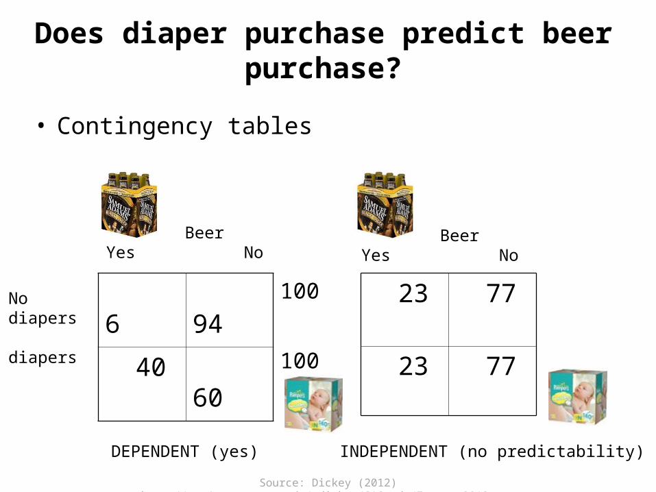
Does diaper purchase predict beer purchase?
• Contingency tables
6 94
40 60
BeerYes No
No diapers
diapers
100
100
DEPENDENT (yes)
23 77
23 77
INDEPENDENT (no predictability)
BeerYes No
Source: Dickey (2012) http://www4.stat.ncsu.edu/~dickey/SAScode/Encore_2012.ppt

56
Support (A B) = P(A B)
Confidence (A B) = P(B|A)Conf (A B) = Supp (A B)/ Supp (A)
Lift (A B) = Supp (A B) / (Supp (A) x Supp (B))Lift (Correlation)
Lift (AB) = Confidence (AB) / Support(B)
Source: Dickey (2012) http://www4.stat.ncsu.edu/~dickey/SAScode/Encore_2012.ppt
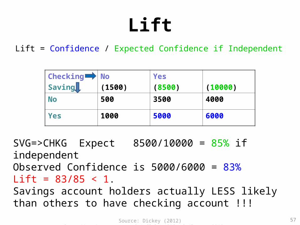
LiftLift = Confidence / Expected Confidence if Independent
57
Checking
Saving
No
(1500)
Yes
(8500) (10000)
No 500 3500 4000
Yes 1000 5000 6000
SVG=>CHKG Expect 8500/10000 = 85% if independentObserved Confidence is 5000/6000 = 83%Lift = 83/85 < 1. Savings account holders actually LESS likely than others to have checking account !!!
Source: Dickey (2012) http://www4.stat.ncsu.edu/~dickey/SAScode/Encore_2012.ppt
• Rules that satisfy both a minimum support threshold (min_sup) and a minimum confidence threshold (min_conf) are called strong.
• By convention, we write support and confidence values so as to occur between 0% and 100%, rather than 0 to 1.0.
58Source: Han & Kamber (2006)
• itemset– A set of items is referred to as an itemset.
• K-itemset– An itemset that contains k items is a k-itemset.
• Example:– The set {computer, antivirus software} is a 2-itemset.
59Source: Han & Kamber (2006)
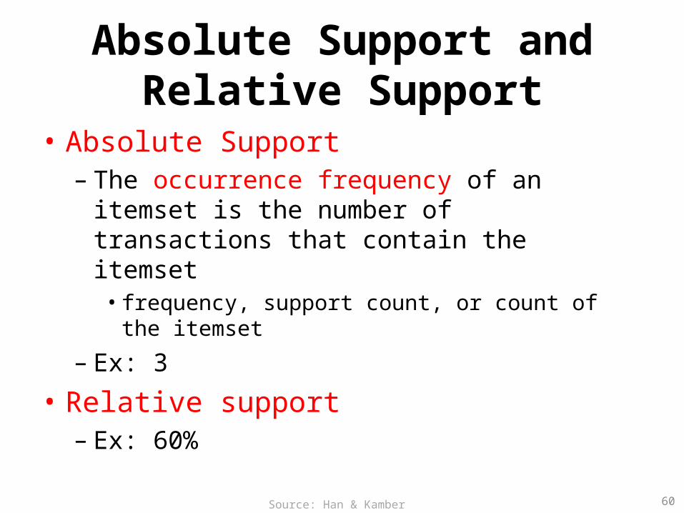
Absolute Support andRelative Support
• Absolute Support – The occurrence frequency of an itemset is the
number of transactions that contain the itemset• frequency, support count, or count of the itemset
– Ex: 3
• Relative support – Ex: 60%
60Source: Han & Kamber (2006)
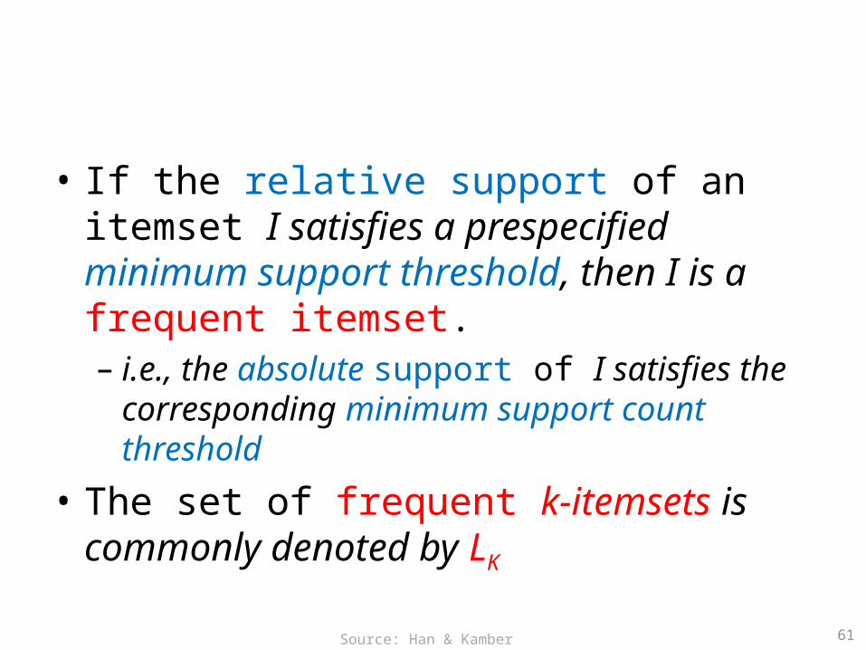
• If the relative support of an itemset I satisfies a prespecified minimum support threshold, then I is a frequent itemset.– i.e., the absolute support of I satisfies the
corresponding minimum support count threshold
• The set of frequent k-itemsets is commonly denoted by LK
61Source: Han & Kamber (2006)
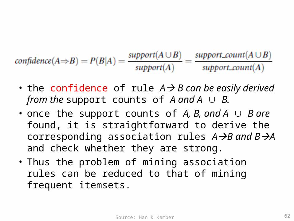
• the confidence of rule A B can be easily derived from the support counts of A and A B.
• once the support counts of A, B, and A B are found, it is straightforward to derive the corresponding association rules AB and BA and check whether they are strong.
• Thus the problem of mining association rules can be reduced to that of mining frequent itemsets.
62Source: Han & Kamber (2006)
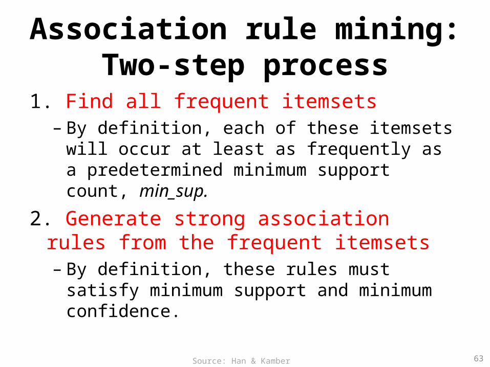
Association rule mining:Two-step process
1. Find all frequent itemsets– By definition, each of these itemsets will occur at
least as frequently as a predetermined minimum support count, min_sup.
2. Generate strong association rules from the frequent itemsets– By definition, these rules must satisfy minimum
support and minimum confidence.
63Source: Han & Kamber (2006)

Efficient and Scalable Frequent Itemset Mining Methods• The Apriori Algorithm
– Finding Frequent Itemsets Using Candidate Generation
64Source: Han & Kamber (2006)

Apriori Algorithm
• Apriori is a seminal algorithm proposed by R. Agrawal and R. Srikant in 1994 for mining frequent itemsets for Boolean association rules.
• The name of the algorithm is based on the fact that the algorithm uses prior knowledge of frequent itemset properties, as we shall see following.
65Source: Han & Kamber (2006)

Apriori Algorithm
• Apriori employs an iterative approach known as a level-wise search, where k-itemsets are used to explore (k+1)-itemsets.
• First, the set of frequent 1-itemsets is found by scanning the database to accumulate the count for each item, and collecting those items that satisfy minimum support. The resulting set is denoted L1.
• Next, L1 is used to find L2, the set of frequent 2-itemsets, which is used to find L3, and so on, until no more frequent k-itemsets can be found.
• The finding of each Lk requires one full scan of the database.
66Source: Han & Kamber (2006)

Apriori Algorithm
• To improve the efficiency of the level-wise generation of frequent itemsets, an important property called the Apriori property.
• Apriori property– All nonempty subsets of a frequent itemset must
also be frequent.
67Source: Han & Kamber (2006)
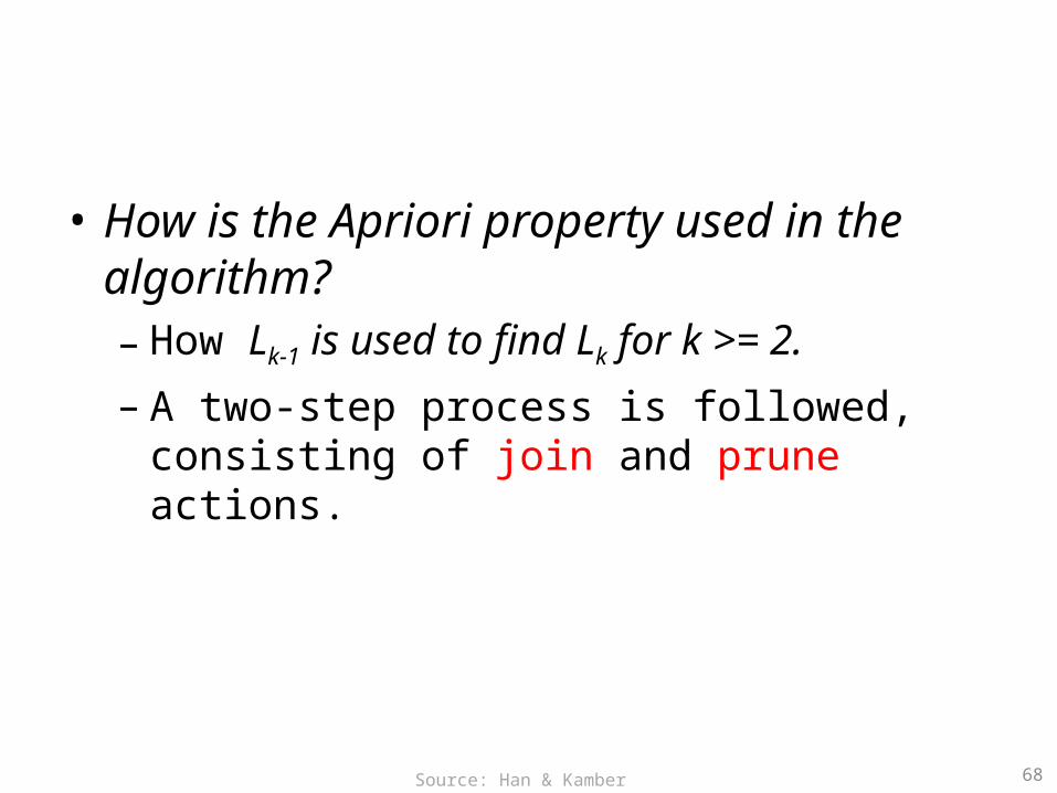
• How is the Apriori property used in the algorithm?– How Lk-1 is used to find Lk for k >= 2.
– A two-step process is followed, consisting of join and prune actions.
68Source: Han & Kamber (2006)
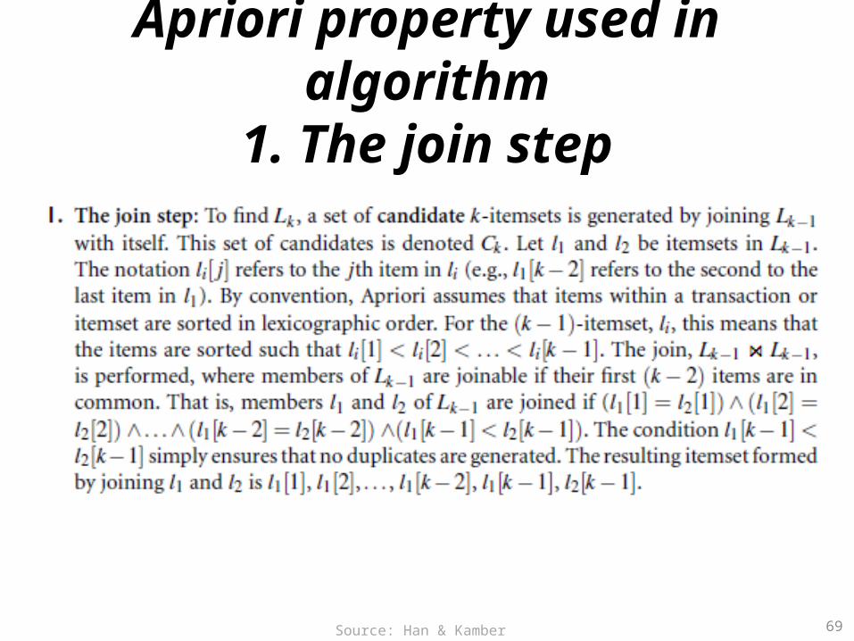
Apriori property used in algorithm1. The join step
69Source: Han & Kamber (2006)

Apriori property used in algorithm2. The prune step
70Source: Han & Kamber (2006)
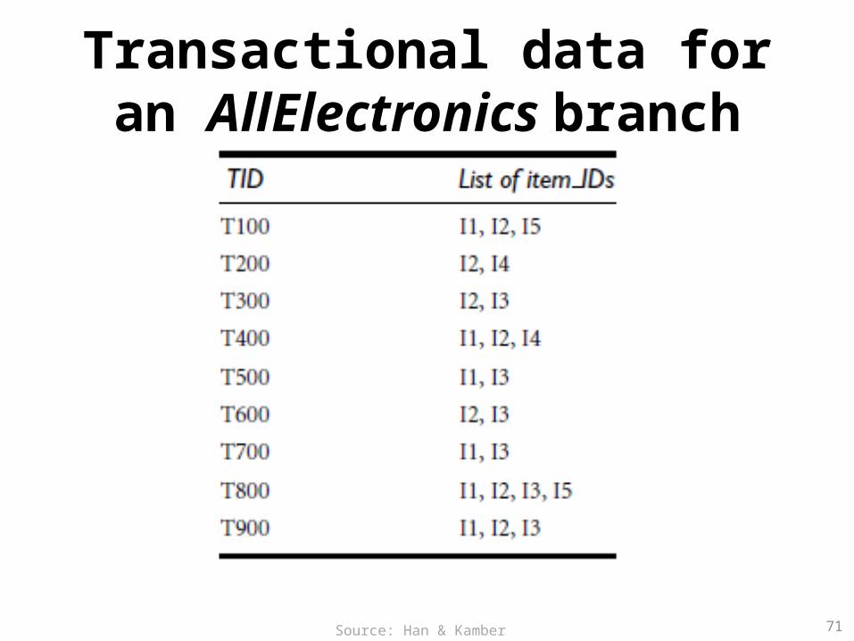
Transactional data for an AllElectronics branch
71Source: Han & Kamber (2006)

Example: Apriori
• Let’s look at a concrete example, based on the AllElectronics transaction database, D.
• There are nine transactions in this database, that is, |D| = 9.
• Apriori algorithm for finding frequent itemsets in D
72Source: Han & Kamber (2006)
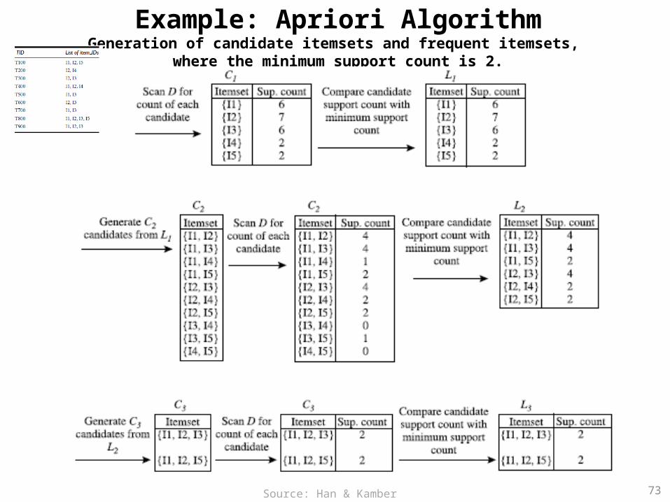
Example: Apriori AlgorithmGeneration of candidate itemsets and frequent itemsets,
where the minimum support count is 2.
73Source: Han & Kamber (2006)

74
Example: Apriori AlgorithmC1 L1
Source: Han & Kamber (2006)
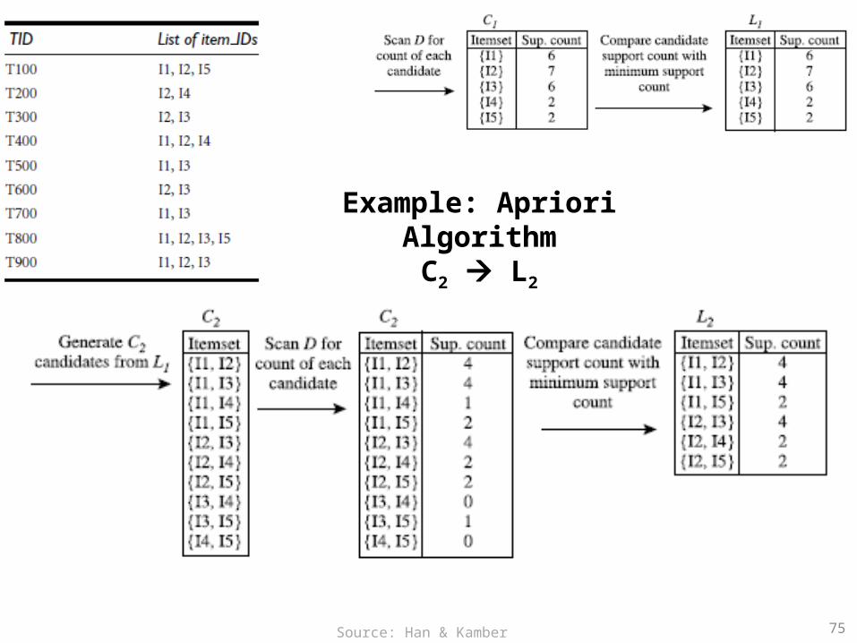
75
Example: Apriori AlgorithmC2 L2
Source: Han & Kamber (2006)

76
Example: Apriori AlgorithmC3 L3
Source: Han & Kamber (2006)
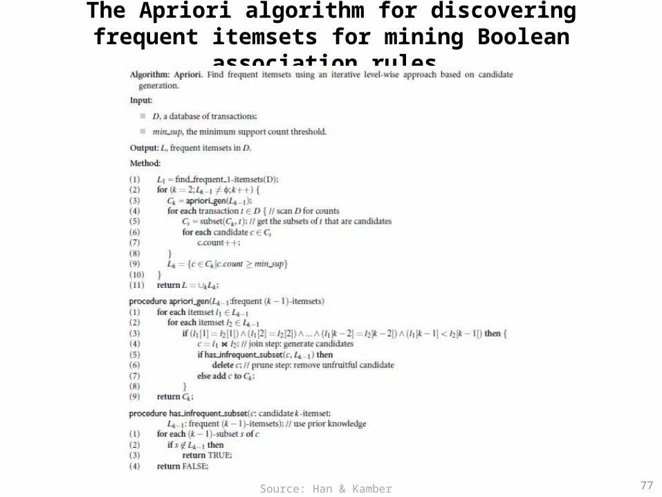
The Apriori algorithm for discovering frequent itemsets for mining Boolean association rules.
77Source: Han & Kamber (2006)
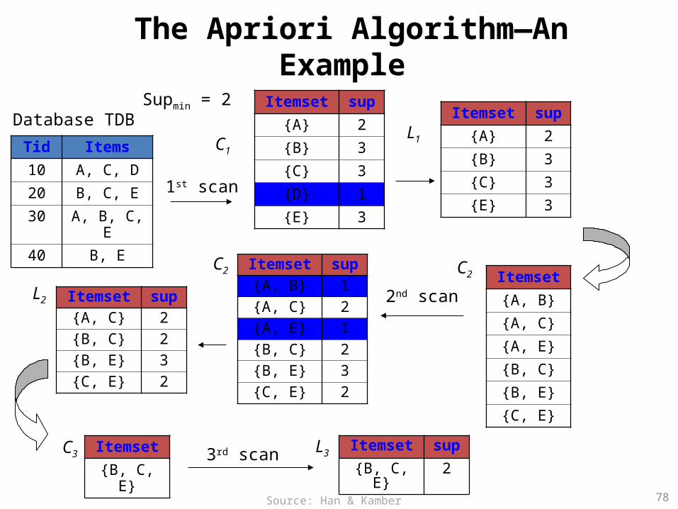
78
The Apriori Algorithm—An Example
Database TDB
1st scan
C1
L1
L2
C2 C2
2nd scan
C3 L33rd scan
Tid Items
10 A, C, D
20 B, C, E
30 A, B, C, E
40 B, E
Itemset sup
{A} 2
{B} 3
{C} 3
{D} 1
{E} 3
Itemset sup
{A} 2
{B} 3
{C} 3
{E} 3
Itemset
{A, B}
{A, C}
{A, E}
{B, C}
{B, E}
{C, E}
Itemset sup{A, B} 1{A, C} 2{A, E} 1{B, C} 2{B, E} 3{C, E} 2
Itemset sup{A, C} 2{B, C} 2{B, E} 3{C, E} 2
Itemset
{B, C, E}
Itemset sup
{B, C, E} 2
Supmin = 2
Source: Han & Kamber (2006)
79
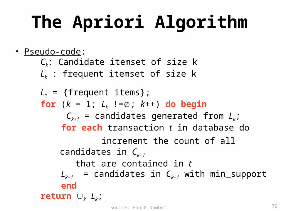
The Apriori Algorithm
• Pseudo-code:Ck: Candidate itemset of size kLk : frequent itemset of size k
L1 = {frequent items};for (k = 1; Lk !=; k++) do begin Ck+1 = candidates generated from Lk; for each transaction t in database do
increment the count of all candidates in Ck+1 that are contained in t
Lk+1 = candidates in Ck+1 with min_support endreturn k Lk;
Source: Han & Kamber (2006)
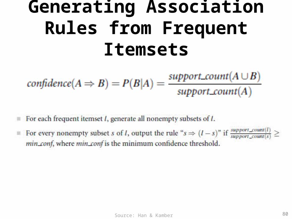
Generating Association Rules from Frequent Itemsets
80Source: Han & Kamber (2006)
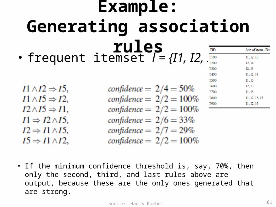
Example:Generating association rules
• frequent itemset l = {I1, I2, I5}
81
• If the minimum confidence threshold is, say, 70%, then only the second, third, and last rules above are output, because these are the only ones generated that are strong.
Source: Han & Kamber (2006)

Classification Techniques• Decision tree analysis• Statistical analysis• Neural networks• Support vector machines• Case-based reasoning• Bayesian classifiers• Genetic algorithms• Rough sets
Source: Turban et al. (2011), Decision Support and Business Intelligence Systems 82
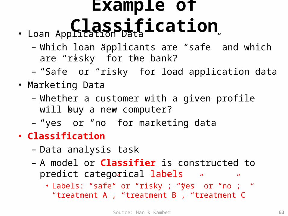
Example of Classification• Loan Application Data
– Which loan applicants are “safe” and which are “risky” for the bank?
– “Safe” or “risky” for load application data• Marketing Data
– Whether a customer with a given profile will buy a new computer?
– “yes” or “no” for marketing data• Classification
– Data analysis task– A model or Classifier is constructed to predict categorical
labels• Labels: “safe” or “risky”; “yes” or “no”;
“treatment A”, “treatment B”, “treatment C”83Source: Han & Kamber (2006)
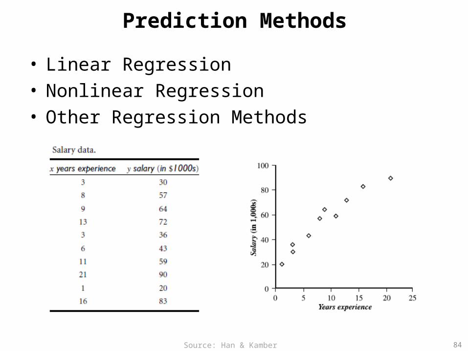
Prediction Methods
• Linear Regression• Nonlinear Regression• Other Regression Methods
84Source: Han & Kamber (2006)
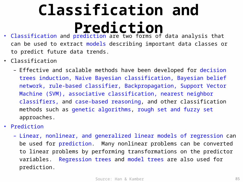
Classification and Prediction• Classification and prediction are two forms of data analysis that can be used to
extract models describing important data classes or to predict future data trends.
• Classification
– Effective and scalable methods have been developed for decision trees induction, Naive Bayesian classification, Bayesian belief network, rule-based classifier, Backpropagation, Support Vector Machine (SVM), associative classification, nearest neighbor classifiers, and case-based reasoning, and other classification methods such as genetic algorithms, rough set and fuzzy set approaches.
• Prediction
– Linear, nonlinear, and generalized linear models of regression can be used for prediction. Many nonlinear problems can be converted to linear problems by performing transformations on the predictor variables. Regression trees and model trees are also used for prediction.
85Source: Han & Kamber (2006)
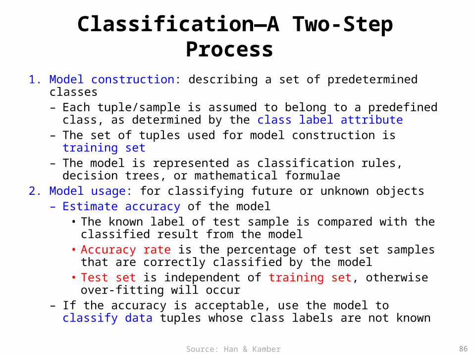
Classification—A Two-Step Process
1. Model construction: describing a set of predetermined classes– Each tuple/sample is assumed to belong to a predefined class, as
determined by the class label attribute– The set of tuples used for model construction is training set– The model is represented as classification rules, decision trees, or
mathematical formulae2. Model usage: for classifying future or unknown objects
– Estimate accuracy of the model• The known label of test sample is compared with the classified
result from the model• Accuracy rate is the percentage of test set samples that are
correctly classified by the model• Test set is independent of training set, otherwise over-fitting will
occur– If the accuracy is acceptable, use the model to classify data tuples
whose class labels are not known
86Source: Han & Kamber (2006)
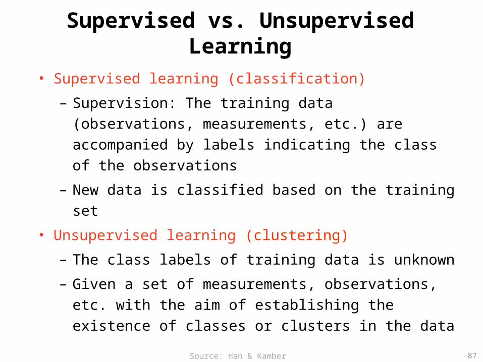
Supervised vs. Unsupervised Learning
• Supervised learning (classification)
– Supervision: The training data (observations, measurements, etc.) are accompanied by labels indicating the class of the observations
– New data is classified based on the training set
• Unsupervised learning (clustering)
– The class labels of training data is unknown
– Given a set of measurements, observations, etc. with the aim of establishing the existence of classes or clusters in the data
87Source: Han & Kamber (2006)
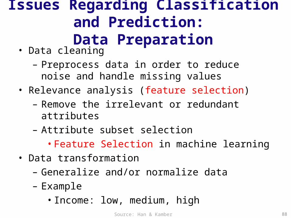
Issues Regarding Classification and Prediction:
Data Preparation• Data cleaning
– Preprocess data in order to reduce noise and handle missing values
• Relevance analysis (feature selection)– Remove the irrelevant or redundant attributes– Attribute subset selection
• Feature Selection in machine learning• Data transformation
– Generalize and/or normalize data– Example
• Income: low, medium, high
88Source: Han & Kamber (2006)
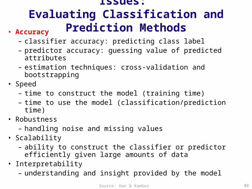
Issues: Evaluating Classification and Prediction Methods
• Accuracy– classifier accuracy: predicting class label– predictor accuracy: guessing value of predicted attributes– estimation techniques: cross-validation and bootstrapping
• Speed– time to construct the model (training time)– time to use the model (classification/prediction time)
• Robustness– handling noise and missing values
• Scalability– ability to construct the classifier or predictor efficiently given
large amounts of data• Interpretability
– understanding and insight provided by the model89Source: Han & Kamber (2006)
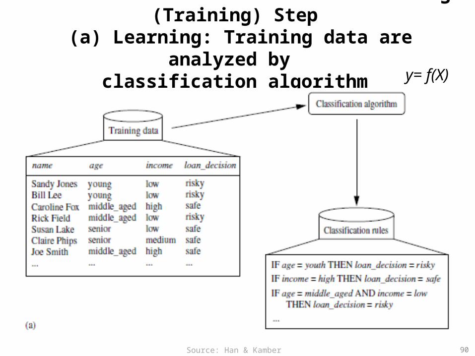
Data Classification Process 1: Learning (Training) Step (a) Learning: Training data are analyzed by
classification algorithmy= f(X)
90Source: Han & Kamber (2006)
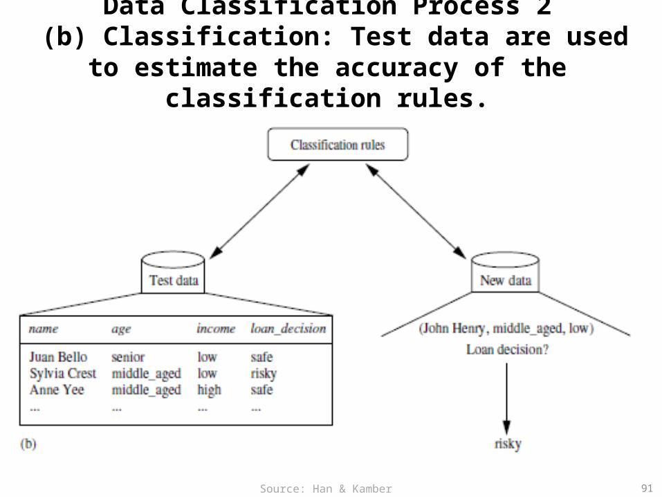
Data Classification Process 2 (b) Classification: Test data are used to estimate the
accuracy of the classification rules.
91Source: Han & Kamber (2006)

Process (1): Model Construction
TrainingData
NAME RANK YEARS TENUREDMike Assistant Prof 3 noMary Assistant Prof 7 yesBill Professor 2 yesJim Associate Prof 7 yesDave Assistant Prof 6 noAnne Associate Prof 3 no
ClassificationAlgorithms
IF rank = ‘professor’OR years > 6THEN tenured = ‘yes’
Classifier(Model)
92Source: Han & Kamber (2006)

Process (2): Using the Model in Prediction
Classifier
TestingData
NAME RANK YEARS TENUREDTom Assistant Prof 2 noMerlisa Associate Prof 7 noGeorge Professor 5 yesJoseph Assistant Prof 7 yes
Unseen Data
(Jeff, Professor, 4)
Tenured?
93Source: Han & Kamber (2006)
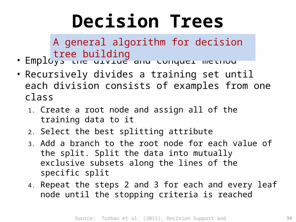
Decision Trees
• Employs the divide and conquer method• Recursively divides a training set until each division
consists of examples from one class1. Create a root node and assign all of the training data to it2. Select the best splitting attribute3. Add a branch to the root node for each value of the split.
Split the data into mutually exclusive subsets along the lines of the specific split
4. Repeat the steps 2 and 3 for each and every leaf node until the stopping criteria is reached
A general algorithm for decision tree building
Source: Turban et al. (2011), Decision Support and Business Intelligence Systems 94

Decision Trees • DT algorithms mainly differ on
– Splitting criteria• Which variable to split first?• What values to use to split?• How many splits to form for each node?
– Stopping criteria• When to stop building the tree
– Pruning (generalization method)• Pre-pruning versus post-pruning
• Most popular DT algorithms include– ID3, C4.5, C5; CART; CHAID; M5
Source: Turban et al. (2011), Decision Support and Business Intelligence Systems 95
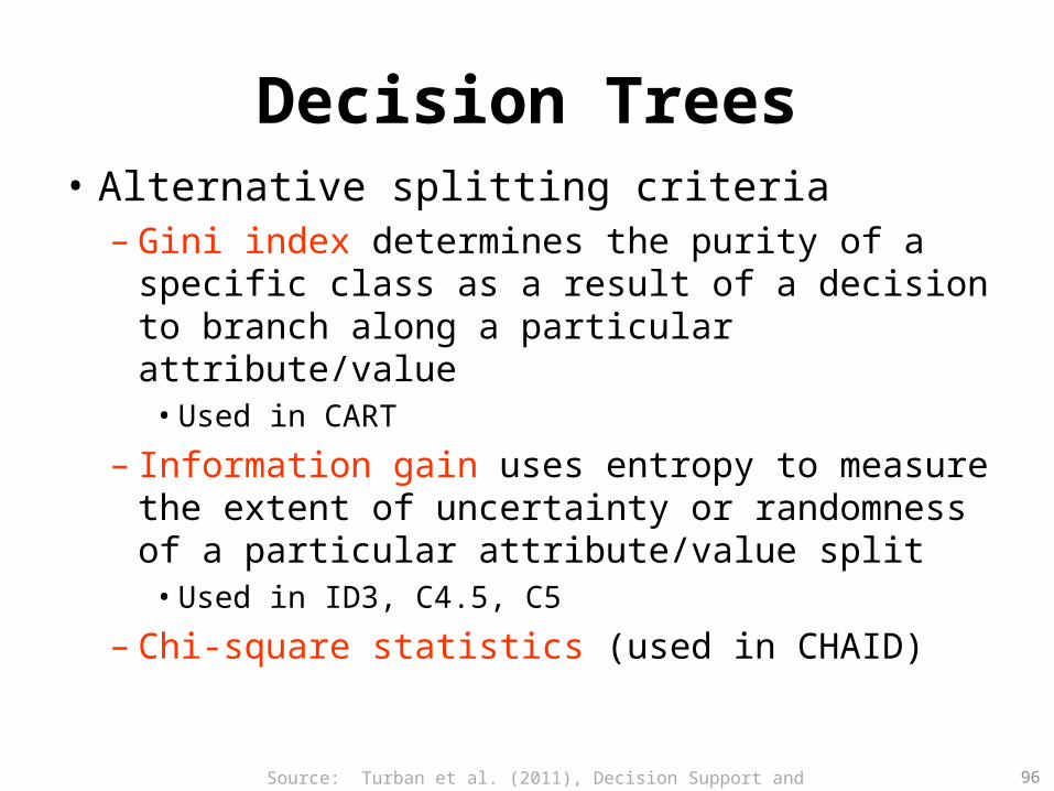
Decision Trees• Alternative splitting criteria
– Gini index determines the purity of a specific class as a result of a decision to branch along a particular attribute/value
• Used in CART
– Information gain uses entropy to measure the extent of uncertainty or randomness of a particular attribute/value split
• Used in ID3, C4.5, C5
– Chi-square statistics (used in CHAID)
Source: Turban et al. (2011), Decision Support and Business Intelligence Systems 96
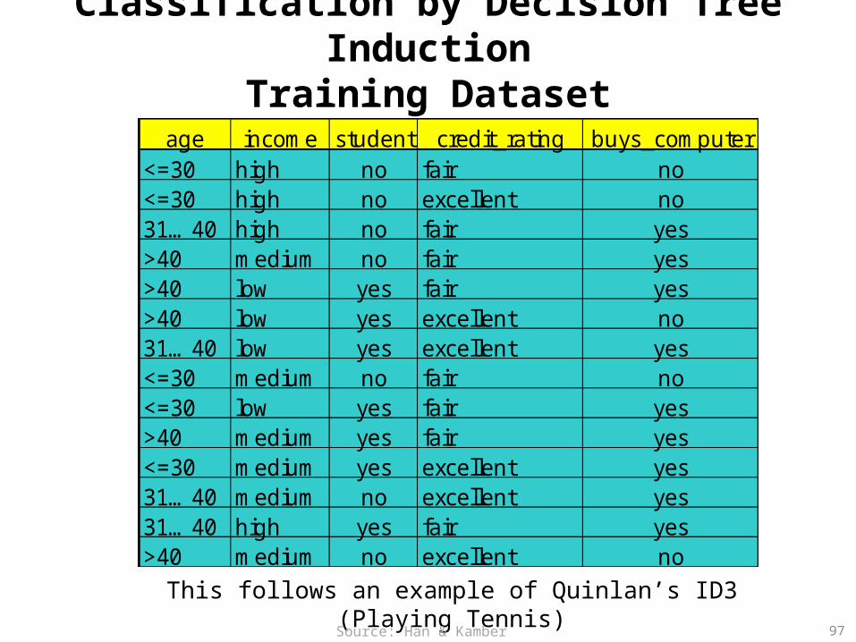
Classification by Decision Tree InductionTraining Dataset
age income student credit_rating buys_computer<=30 high no fair no<=30 high no excellent no31…40 high no fair yes>40 medium no fair yes>40 low yes fair yes>40 low yes excellent no31…40 low yes excellent yes<=30 medium no fair no<=30 low yes fair yes>40 medium yes fair yes<=30 medium yes excellent yes31…40 medium no excellent yes31…40 high yes fair yes>40 medium no excellent no
This follows an example of Quinlan’s ID3 (Playing Tennis)
97Source: Han & Kamber (2006)
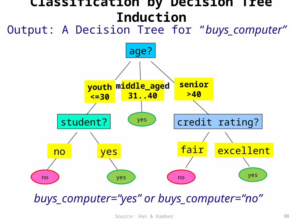
Output: A Decision Tree for “buys_computer”
age?
student? credit rating?
youth<=30
senior>40
middle_aged31..40
fair excellentyesno
Classification by Decision Tree Induction
buys_computer=“yes” or buys_computer=“no”
yes
yes yesnono
98Source: Han & Kamber (2006)
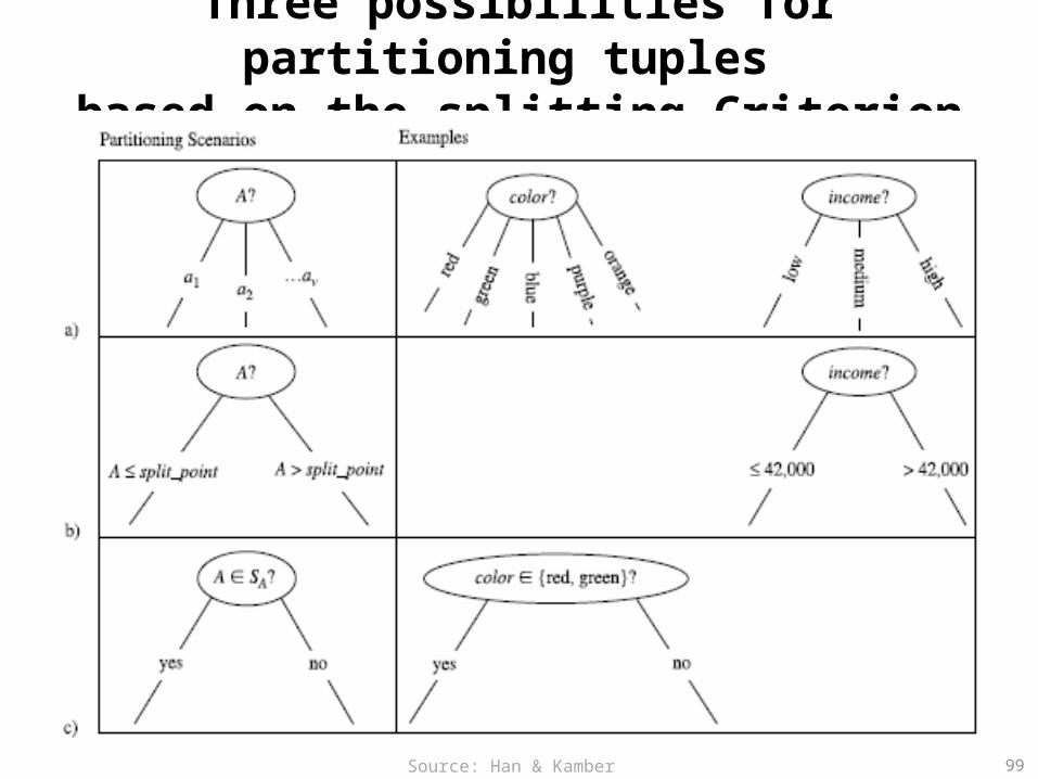
Three possibilities for partitioning tuples based on the splitting Criterion
99Source: Han & Kamber (2006)

Algorithm for Decision Tree Induction• Basic algorithm (a greedy algorithm)
– Tree is constructed in a top-down recursive divide-and-conquer manner– At start, all the training examples are at the root– Attributes are categorical (if continuous-valued, they are discretized in
advance)– Examples are partitioned recursively based on selected attributes– Test attributes are selected on the basis of a heuristic or statistical
measure (e.g., information gain)• Conditions for stopping partitioning
– All samples for a given node belong to the same class– There are no remaining attributes for further partitioning –
majority voting is employed for classifying the leaf– There are no samples left
100Source: Han & Kamber (2006)
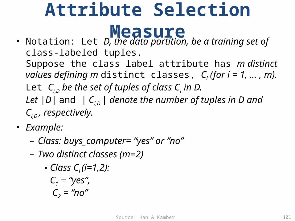
Attribute Selection Measure• Notation: Let D, the data partition, be a training set of class-
labeled tuples. Suppose the class label attribute has m distinct values defining m distinct classes, Ci (for i = 1, … , m). Let Ci,D be the set of tuples of class Ci in D. Let |D| and | Ci,D | denote the number of tuples in D and Ci,D , respectively.
• Example:– Class: buys_computer= “yes” or “no”– Two distinct classes (m=2)
• Class Ci (i=1,2): C1 = “yes”, C2 = “no”
101Source: Han & Kamber (2006)

Attribute Selection Measure: Information Gain (ID3/C4.5)
Select the attribute with the highest information gain Let pi be the probability that an arbitrary tuple in D belongs
to class Ci, estimated by |Ci, D|/|D| Expected information (entropy) needed to classify a tuple
in D:
Information needed (after using A to split D into v partitions) to classify D:
Information gained by branching on attribute A
)(log)( 21
i
m
ii ppDInfo
)(||
||)(
1j
v
j
jA DI
D
DDInfo
(D)InfoInfo(D)Gain(A) A
102Source: Han & Kamber (2006)
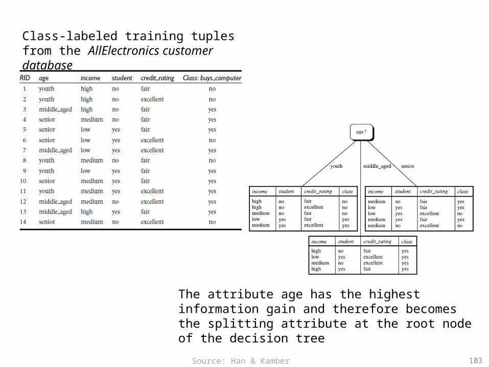
The attribute age has the highest information gain and therefore becomes the splitting attribute at the root node of the decision tree
Class-labeled training tuples from the AllElectronics customer database
103Source: Han & Kamber (2006)
104Source: Han & Kamber (2006)
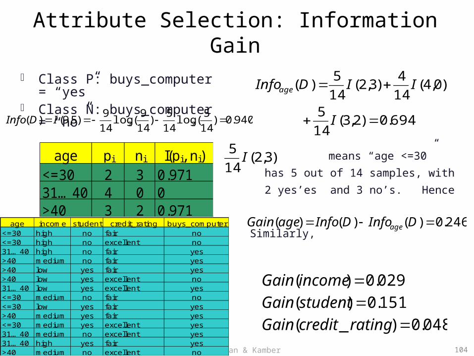
Attribute Selection: Information Gain
Class P: buys_computer = “yes” Class N: buys_computer = “no”
means “age <=30” has 5 out of
14 samples, with 2 yes’es and 3
no’s. Hence
Similarly,
age pi ni I(pi, ni)<=30 2 3 0.97131…40 4 0 0>40 3 2 0.971
694.0)2,3(14
5
)0,4(14
4)3,2(
14
5)(
I
IIDInfoage
048.0)_(
151.0)(
029.0)(
ratingcreditGain
studentGain
incomeGain
246.0)()()( DInfoDInfoageGain ageage income student credit_rating buys_computer
<=30 high no fair no<=30 high no excellent no31…40 high no fair yes>40 medium no fair yes>40 low yes fair yes>40 low yes excellent no31…40 low yes excellent yes<=30 medium no fair no<=30 low yes fair yes>40 medium yes fair yes<=30 medium yes excellent yes31…40 medium no excellent yes31…40 high yes fair yes>40 medium no excellent no
)3,2(14
5I
940.0)14
5(log
14
5)
14
9(log
14
9)5,9()( 22 IDInfo
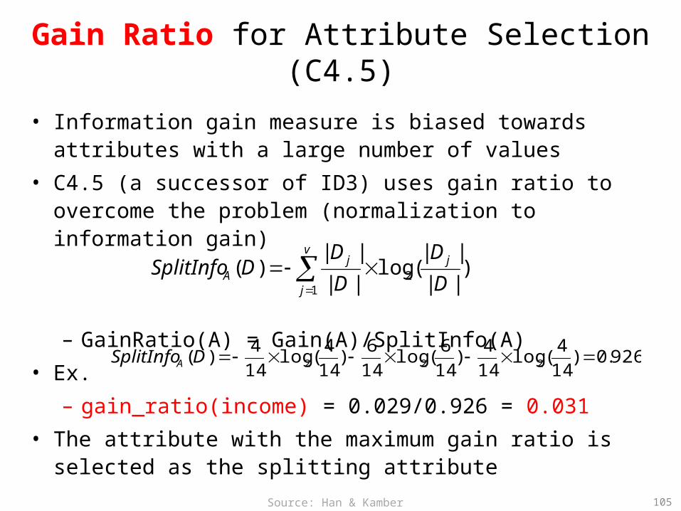
Gain Ratio for Attribute Selection (C4.5)
• Information gain measure is biased towards attributes with a large number of values
• C4.5 (a successor of ID3) uses gain ratio to overcome the problem (normalization to information gain)
– GainRatio(A) = Gain(A)/SplitInfo(A)• Ex.
– gain_ratio(income) = 0.029/0.926 = 0.031• The attribute with the maximum gain ratio is selected as the
splitting attribute
)||
||(log
||
||)( 2
1 D
D
D
DDSplitInfo j
v
j
jA
926.0)14
4(log
14
4)
14
6(log
14
6)
14
4(log
14
4)( 222 DSplitInfoA
105Source: Han & Kamber (2006)
Trees
• A “divisive” method (splits) • Start with “root node” – all in one group• Get splitting rules• Response often binary• Result is a “tree”• Example: Loan Defaults• Example: Framingham Heart Study• Example: Automobile fatalities
Source: Dickey (2012) http://www4.stat.ncsu.edu/~dickey/SAScode/Encore_2012.ppt
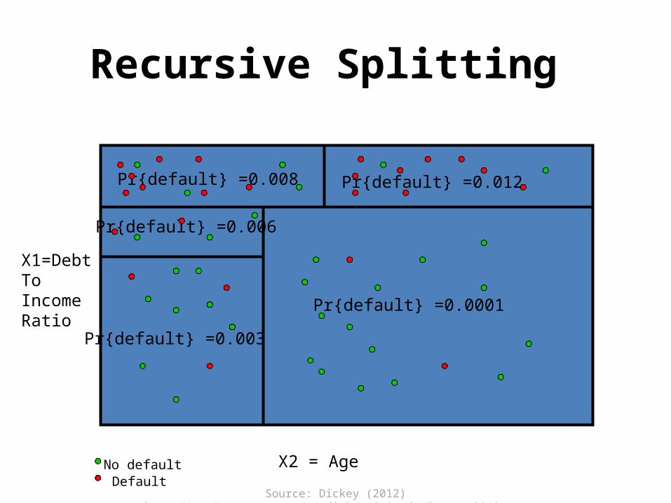
Recursive Splitting
X1=DebtToIncomeRatio
X2 = Age
Pr{default} =0.008 Pr{default} =0.012
Pr{default} =0.0001
Pr{default} =0.003
Pr{default} =0.006
No defaultDefault
Source: Dickey (2012) http://www4.stat.ncsu.edu/~dickey/SAScode/Encore_2012.ppt
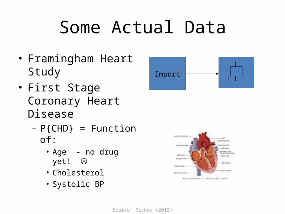
Some Actual Data
• Framingham Heart Study
• First Stage Coronary Heart Disease – P{CHD} = Function of:
• Age - no drug yet! • Cholesterol• Systolic BP
Import
Source: Dickey (2012) http://www4.stat.ncsu.edu/~dickey/SAScode/Encore_2012.ppt
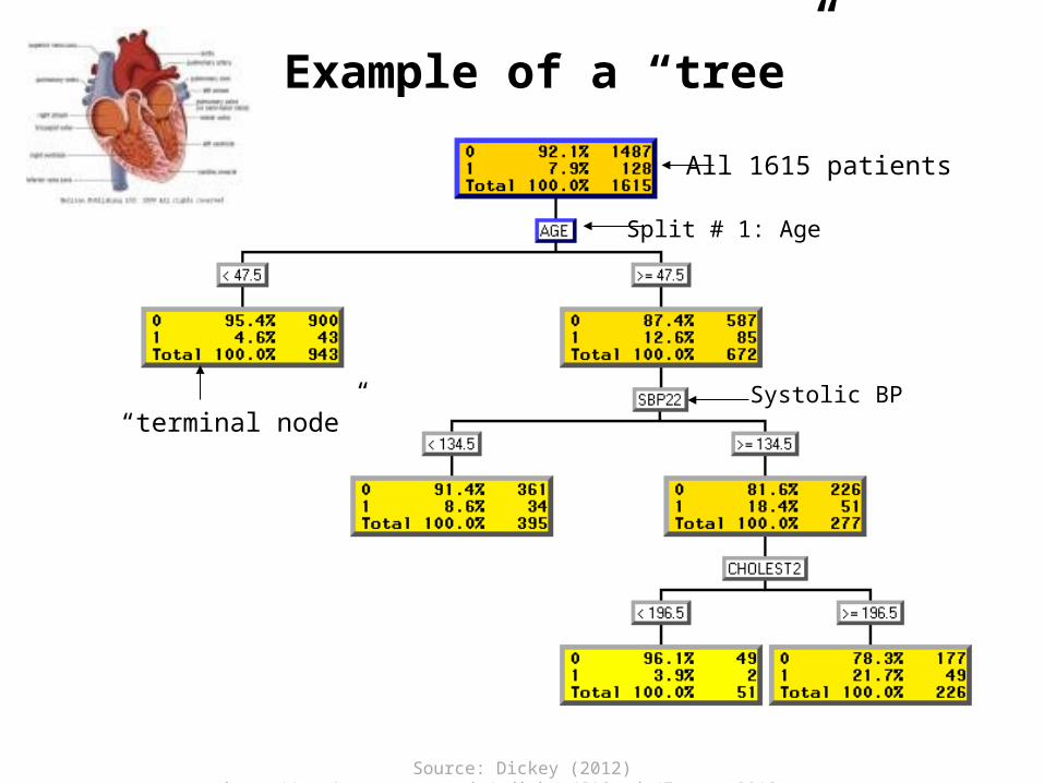
Example of a “tree”
All 1615 patients
Split # 1: Age
“terminal node”Systolic BP
Source: Dickey (2012) http://www4.stat.ncsu.edu/~dickey/SAScode/Encore_2012.ppt
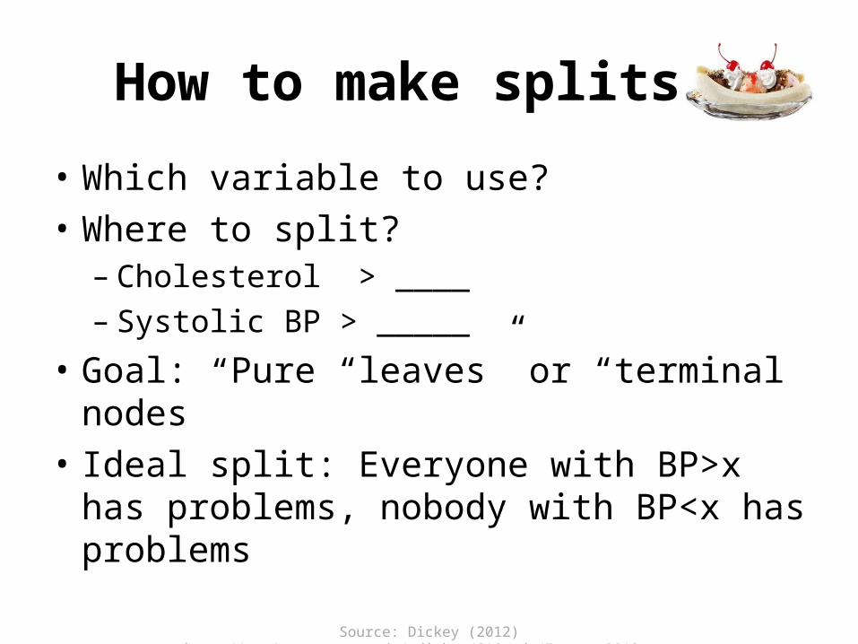
How to make splits?
• Which variable to use? • Where to split?
– Cholesterol > ____– Systolic BP > _____
• Goal: Pure “leaves” or “terminal nodes”• Ideal split: Everyone with BP>x has problems,
nobody with BP<x has problems
Source: Dickey (2012) http://www4.stat.ncsu.edu/~dickey/SAScode/Encore_2012.ppt
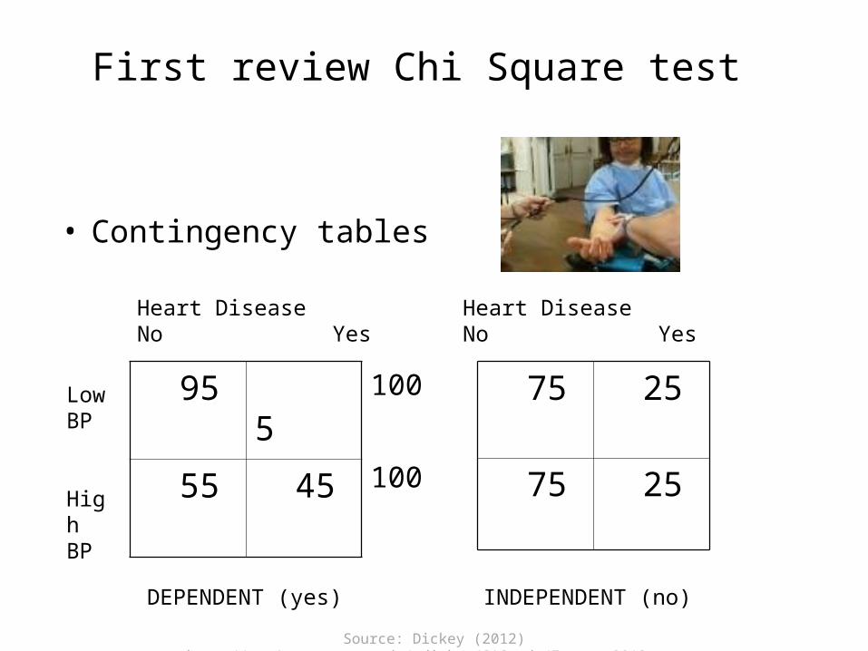
First review Chi Square test
• Contingency tables
95 5
55 45
Heart DiseaseNo Yes
LowBP
HighBP
100
100
DEPENDENT (yes)
75 25
75 25
INDEPENDENT (no)
Heart DiseaseNo Yes
Source: Dickey (2012) http://www4.stat.ncsu.edu/~dickey/SAScode/Encore_2012.ppt
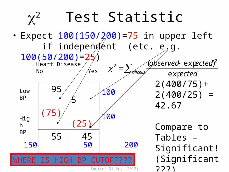
2 Test Statistic • Expect 100(150/200)=75 in upper left
if independent (etc. e.g. 100(50/200)=25)
95
(75)
5
(25)
55
(75)
45
(25)
Heart DiseaseNo Yes
LowBP
HighBP
100
100
150 50 200
allcells ected
ectedobserved
exp
)exp( 22
2(400/75)+2(400/25) = 42.67
Compare to Tables – Significant!(Significant ???)WHERE IS HIGH BP CUTOFF???
Source: Dickey (2012) http://www4.stat.ncsu.edu/~dickey/SAScode/Encore_2012.ppt
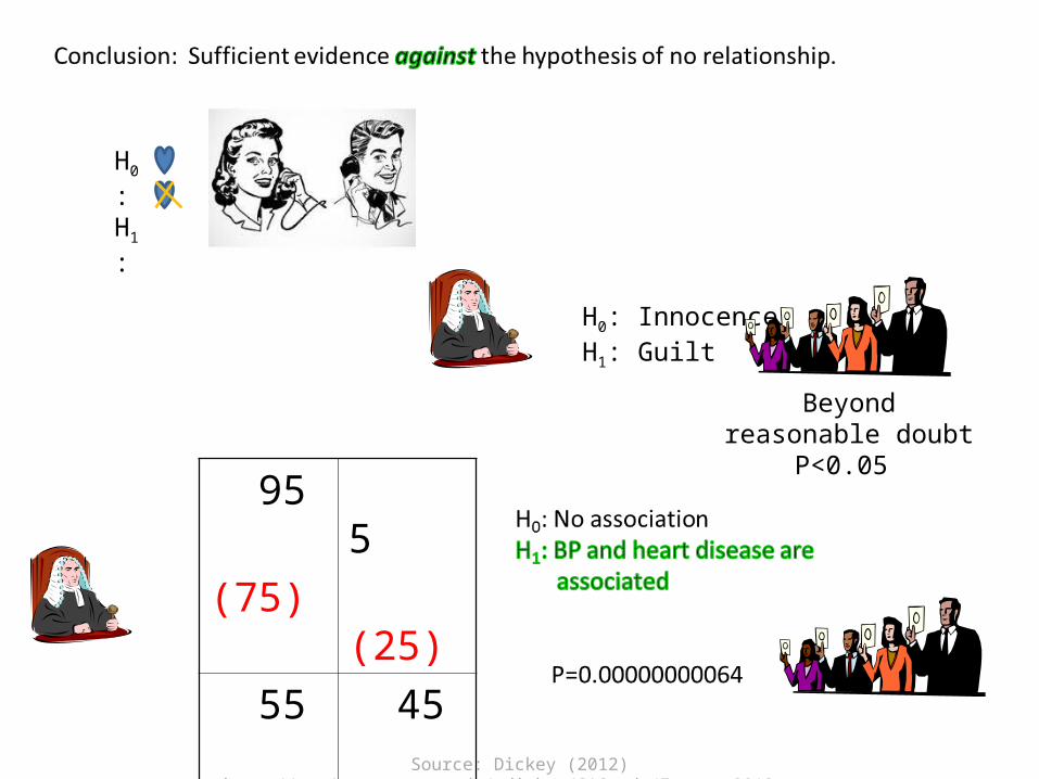
H0:H1:
H0: InnocenceH1: Guilt
Beyond reasonable doubt
P<0.05 95
(75)
5
(25)
55
(75)
45
(25)
Source: Dickey (2012) http://www4.stat.ncsu.edu/~dickey/SAScode/Encore_2012.ppt
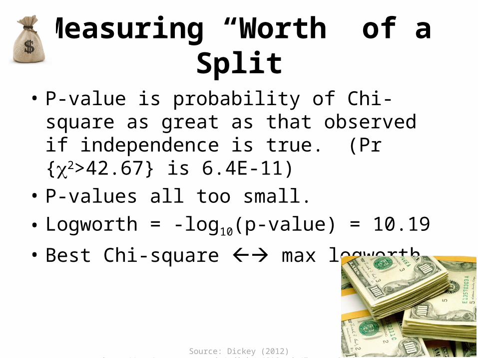
Measuring “Worth” of a Split
• P-value is probability of Chi-square as great as that observed if independence is true. (Pr {2>42.67} is 6.4E-11)
• P-values all too small.• Logworth = -log10(p-value) = 10.19
• Best Chi-square max logworth.
Source: Dickey (2012) http://www4.stat.ncsu.edu/~dickey/SAScode/Encore_2012.ppt

Logworth for Age Splits
Age 47 maximizes logworth
?
Source: Dickey (2012) http://www4.stat.ncsu.edu/~dickey/SAScode/Encore_2012.ppt
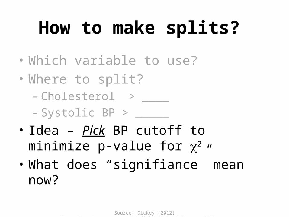
How to make splits?
• Which variable to use? • Where to split?
– Cholesterol > ____– Systolic BP > _____
• Idea – Pick BP cutoff to minimize p-value for 2
• What does “signifiance” mean now?
Source: Dickey (2012) http://www4.stat.ncsu.edu/~dickey/SAScode/Encore_2012.ppt
Cluster Analysis
• Used for automatic identification of natural groupings of things
• Part of the machine-learning family • Employ unsupervised learning• Learns the clusters of things from past data,
then assigns new instances• There is not an output variable• Also known as segmentation
Source: Turban et al. (2011), Decision Support and Business Intelligence Systems 117
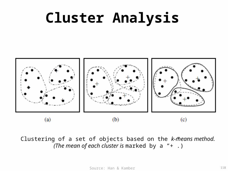
Cluster Analysis
118
Clustering of a set of objects based on the k-means method. (The mean of each cluster is marked by a “+”.)
Source: Han & Kamber (2006)
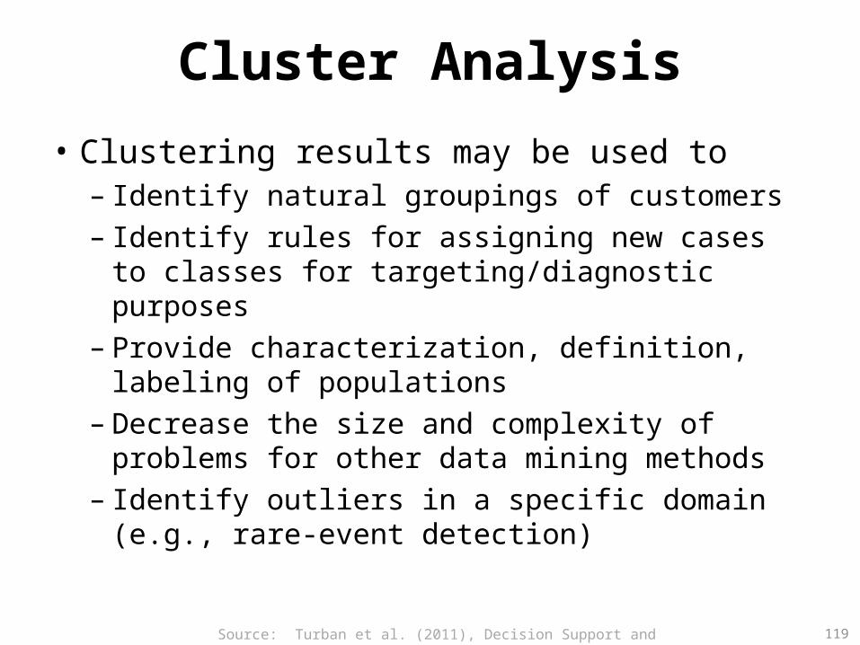
Cluster Analysis
• Clustering results may be used to– Identify natural groupings of customers– Identify rules for assigning new cases to classes for
targeting/diagnostic purposes– Provide characterization, definition, labeling of
populations– Decrease the size and complexity of problems for
other data mining methods – Identify outliers in a specific domain
(e.g., rare-event detection)
Source: Turban et al. (2011), Decision Support and Business Intelligence Systems 119
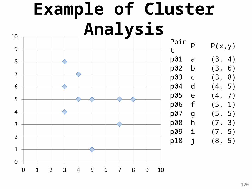
120
Point P P(x,y)p01 a (3, 4)p02 b (3, 6)p03 c (3, 8)p04 d (4, 5)p05 e (4, 7)p06 f (5, 1)p07 g (5, 5)p08 h (7, 3)p09 i (7, 5)p10 j (8, 5)
Example of Cluster Analysis

Cluster Analysis for Data Mining• Analysis methods
– Statistical methods (including both hierarchical and nonhierarchical), such as k-means, k-modes, and so on
– Neural networks (adaptive resonance theory [ART], self-organizing map [SOM])
– Fuzzy logic (e.g., fuzzy c-means algorithm)– Genetic algorithms
• Divisive versus Agglomerative methodsSource: Turban et al. (2011), Decision Support and Business Intelligence Systems 121
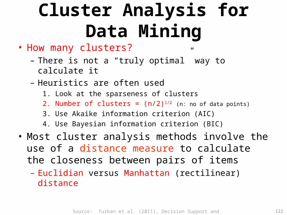
Cluster Analysis for Data Mining• How many clusters?
– There is not a “truly optimal” way to calculate it– Heuristics are often used
1. Look at the sparseness of clusters2. Number of clusters = (n/2)1/2 (n: no of data points)
3. Use Akaike information criterion (AIC)4. Use Bayesian information criterion (BIC)
• Most cluster analysis methods involve the use of a distance measure to calculate the closeness between pairs of items – Euclidian versus Manhattan (rectilinear) distance
Source: Turban et al. (2011), Decision Support and Business Intelligence Systems 122

k-Means Clustering Algorithm• k : pre-determined number of clusters• Algorithm (Step 0: determine value of k)Step 1: Randomly generate k random points as initial
cluster centersStep 2: Assign each point to the nearest cluster centerStep 3: Re-compute the new cluster centersRepetition step: Repeat steps 2 and 3 until some
convergence criterion is met (usually that the assignment of points to clusters becomes stable)
Source: Turban et al. (2011), Decision Support and Business Intelligence Systems 123
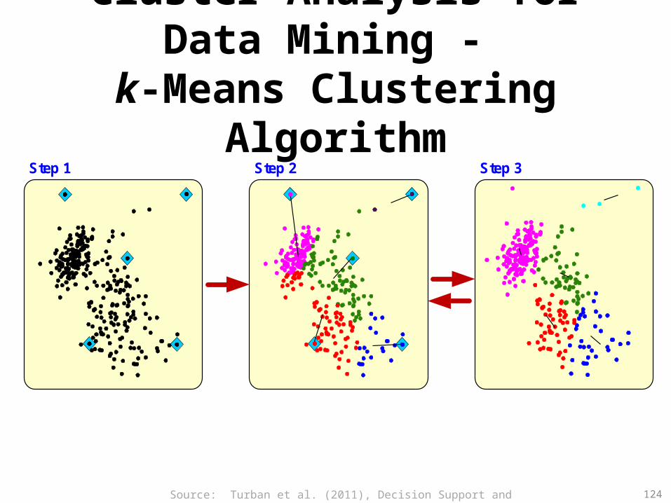
Cluster Analysis for Data Mining - k-Means Clustering Algorithm
Step 1 Step 2 Step 3
Source: Turban et al. (2011), Decision Support and Business Intelligence Systems 124
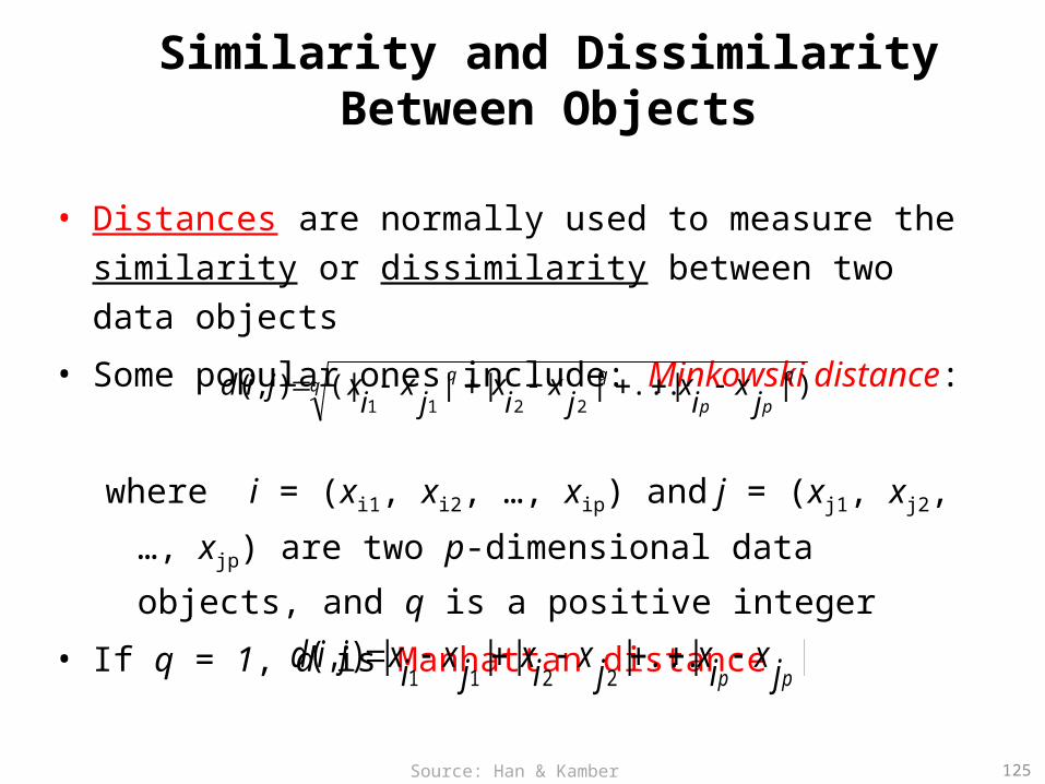
Similarity and Dissimilarity Between Objects
• Distances are normally used to measure the similarity or dissimilarity between two data objects
• Some popular ones include: Minkowski distance:
where i = (xi1, xi2, …, xip) and j = (xj1, xj2, …, xjp) are two p-
dimensional data objects, and q is a positive integer
• If q = 1, d is Manhattan distance
pp
jx
ix
jx
ix
jx
ixjid )||...|||(|),(
2211
||...||||),(2211 pp jxixjxixjxixjid
125Source: Han & Kamber (2006)
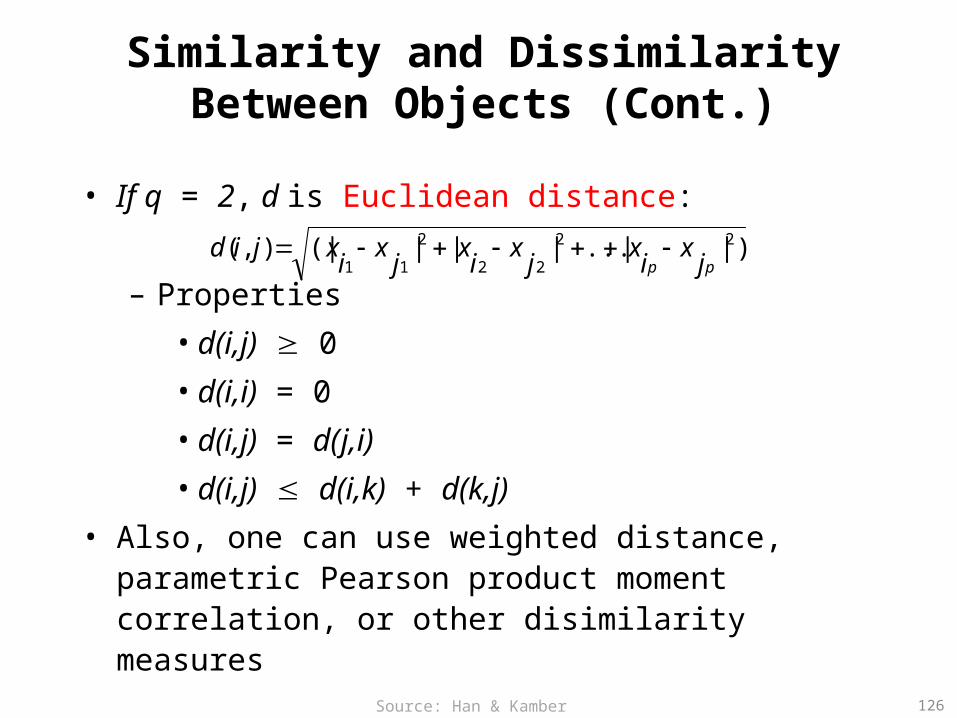
Similarity and Dissimilarity Between Objects (Cont.)
• If q = 2, d is Euclidean distance:
– Properties• d(i,j) 0• d(i,i) = 0• d(i,j) = d(j,i)• d(i,j) d(i,k) + d(k,j)
• Also, one can use weighted distance, parametric Pearson product moment correlation, or other disimilarity measures
)||...|||(|),( 22
22
2
11 pp jx
ix
jx
ix
jx
ixjid
126Source: Han & Kamber (2006)
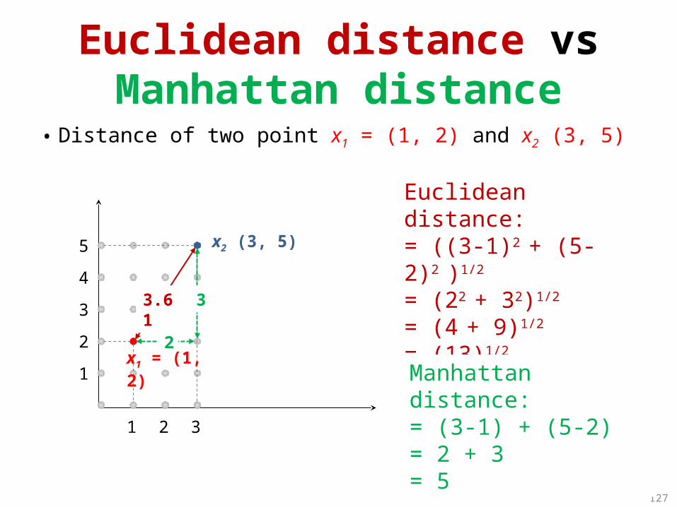
Euclidean distance vs Manhattan distance
• Distance of two point x1 = (1, 2) and x2 (3, 5)
127
1 2 3
1
2
3
4
5 x2 (3, 5)
2x1 = (1, 2)
33.61
Euclidean distance:= ((3-1)2 + (5-2)2 )1/2
= (22 + 32)1/2
= (4 + 9)1/2
= (13)1/2
= 3.61
Manhattan distance:= (3-1) + (5-2)= 2 + 3= 5
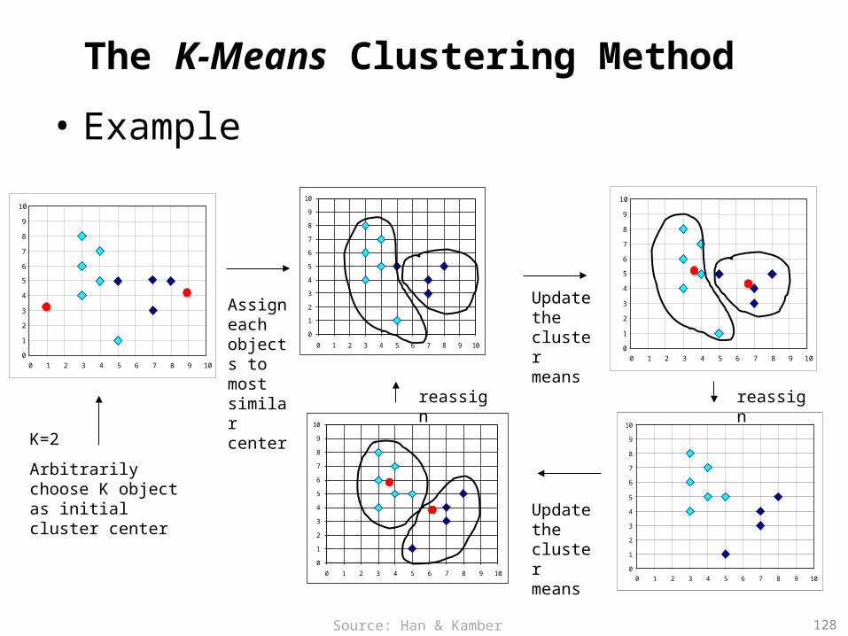
The K-Means Clustering Method
• Example
0
1
2
3
4
5
6
7
8
9
10
0 1 2 3 4 5 6 7 8 9 10 0
1
2
3
4
5
6
7
8
9
10
0 1 2 3 4 5 6 7 8 9 10
0
1
2
3
4
5
6
7
8
9
10
0 1 2 3 4 5 6 7 8 9 10
0
1
2
3
4
5
6
7
8
9
10
0 1 2 3 4 5 6 7 8 9 10
0
1
2
3
4
5
6
7
8
9
10
0 1 2 3 4 5 6 7 8 9 10
K=2
Arbitrarily choose K object as initial cluster center
Assign each objects to most similar center
Update the cluster means
Update the cluster means
reassignreassign
128Source: Han & Kamber (2006)
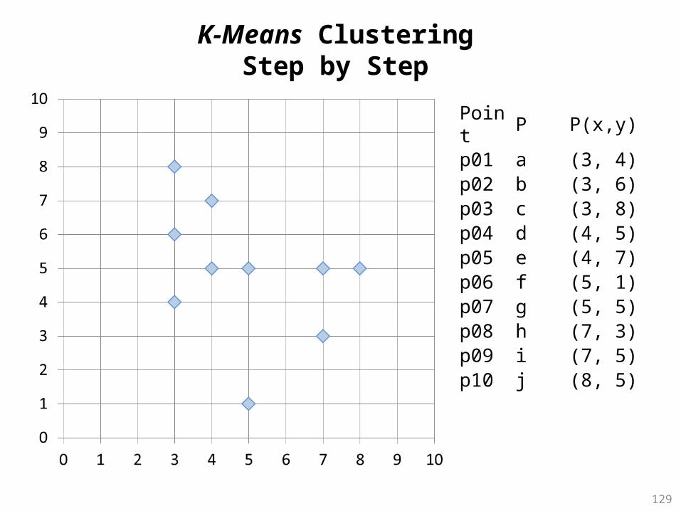
129
Point P P(x,y)p01 a (3, 4)p02 b (3, 6)p03 c (3, 8)p04 d (4, 5)p05 e (4, 7)p06 f (5, 1)p07 g (5, 5)p08 h (7, 3)p09 i (7, 5)p10 j (8, 5)
K-Means ClusteringStep by Step

130
Point P P(x,y)p01 a (3, 4)p02 b (3, 6)p03 c (3, 8)p04 d (4, 5)p05 e (4, 7)p06 f (5, 1)p07 g (5, 5)p08 h (7, 3)p09 i (7, 5)p10 j (8, 5)
Initial m1 (3, 4)Initial m2 (8, 5)
m1 = (3, 4)
M2 = (8, 5)
K-Means ClusteringStep 1: K=2, Arbitrarily choose K object as initial cluster center
131
Point P P(x,y)m1
distance
m2 distanc
eCluster
p01 a(3, 4)
0.00 5.10 Cluster1
p02 b(3, 6)
2.00 5.10 Cluster1
p03 c(3, 8)
4.00 5.83 Cluster1
p04 d(4, 5)
1.41 4.00 Cluster1
p05 e(4, 7)
3.16 4.47 Cluster1
p06 f(5, 1)
3.61 5.00 Cluster1
p07 g(5, 5)
2.24 3.00 Cluster1
p08 h(7, 3)
4.12 2.24 Cluster2
p09 i(7, 5)
4.12 1.00 Cluster2
p10 j(8, 5)
5.10 0.00 Cluster2
Initial
m1(3, 4)
Initial
m2(8, 5)
M2 = (8, 5)
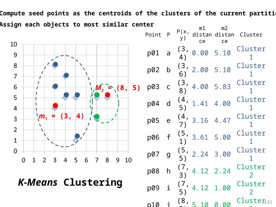
Step 2: Compute seed points as the centroids of the clusters of the current partition
Step 3: Assign each objects to most similar center
m1 = (3, 4)
K-Means Clustering

132
Point P P(x,y)m1
distance
m2 distanc
eCluster
p01 a(3, 4)
0.00 5.10 Cluster1
p02 b(3, 6)
2.00 5.10 Cluster1
p03 c(3, 8)
4.00 5.83 Cluster1
p04 d(4, 5)
1.41 4.00 Cluster1
p05 e(4, 7)
3.16 4.47 Cluster1
p06 f(5, 1)
3.61 5.00 Cluster1
p07 g(5, 5)
2.24 3.00 Cluster1
p08 h(7, 3)
4.12 2.24 Cluster2
p09 i(7, 5)
4.12 1.00 Cluster2
p10 j(8, 5)
5.10 0.00 Cluster2
Initial
m1(3, 4)
Initial
m2(8, 5)
M2 = (8, 5)
Step 2: Compute seed points as the centroids of the clusters of the current partition
Step 3: Assign each objects to most similar center
m1 = (3, 4)
K-Means Clustering
Euclidean distance b(3,6) m2(8,5)= ((8-3)2 + (5-6)2 )1/2
= (52 + (-1)2)1/2
= (25 + 1)1/2
= (26)1/2
= 5.10
Euclidean distance b(3,6) m1(3,4)= ((3-3)2 + (4-6)2 )1/2
= (02 + (-2)2)1/2
= (0 + 4)1/2
= (4)1/2
= 2.00

133
Point P P(x,y)m1
distance
m2 distanc
eCluster
p01 a (3, 4) 1.43 4.34 Cluster
1
p02 b (3, 6) 1.22 4.64 Cluster
1
p03 c (3, 8) 2.99 5.68 Cluster
1
p04 d (4, 5) 0.20 3.40 Cluster
1
p05 e (4, 7) 1.87 4.27 Cluster
1
p06 f (5, 1) 4.29 4.06 Cluster
2
p07 g (5, 5) 1.15 2.42 Cluster
1
p08 h (7, 3) 3.80 1.37 Cluster
2
p09 i (7, 5) 3.14 0.75 Cluster
2
p10 j (8, 5) 4.14 0.95 Cluster
2
m1 (3.86, 5.14)m2 (7.33, 4.33)
m1 = (3.86, 5.14)
M2 = (7.33, 4.33)
Step 4: Update the cluster means, Repeat Step 2, 3, stop when no more new assignment
K-Means Clustering
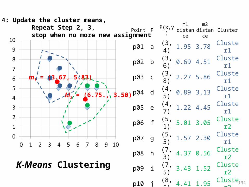
134
Point P P(x,y)m1
distance
m2 distanc
eCluster
p01 a (3, 4) 1.95 3.78 Cluster
1
p02 b (3, 6) 0.69 4.51 Cluster
1
p03 c (3, 8) 2.27 5.86 Cluster
1
p04 d (4, 5) 0.89 3.13 Cluster
1
p05 e (4, 7) 1.22 4.45 Cluster
1
p06 f (5, 1) 5.01 3.05 Cluster
2
p07 g (5, 5) 1.57 2.30 Cluster
1
p08 h (7, 3) 4.37 0.56 Cluster
2
p09 i (7, 5) 3.43 1.52 Cluster
2
p10 j (8, 5) 4.41 1.95 Cluster
2
m1 (3.67, 5.83)m2 (6.75, 3.50)
M2 = (6.75., 3.50)
m1 = (3.67, 5.83)
Step 4: Update the cluster means, Repeat Step 2, 3, stop when no more new assignment
K-Means Clustering

135
Point P P(x,y)m1
distance
m2 distanc
eCluster
p01 a (3, 4) 1.95 3.78 Cluster
1
p02 b (3, 6) 0.69 4.51 Cluster
1
p03 c (3, 8) 2.27 5.86 Cluster
1
p04 d (4, 5) 0.89 3.13 Cluster
1
p05 e (4, 7) 1.22 4.45 Cluster
1
p06 f (5, 1) 5.01 3.05 Cluster
2
p07 g (5, 5) 1.57 2.30 Cluster
1
p08 h (7, 3) 4.37 0.56 Cluster
2
p09 i (7, 5) 3.43 1.52 Cluster
2
p10 j (8, 5) 4.41 1.95 Cluster
2
m1 (3.67, 5.83)m2 (6.75, 3.50)
stop when no more new assignment
K-Means Clustering
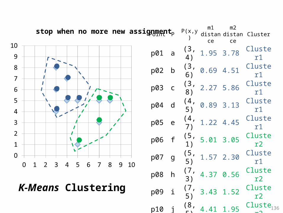
136
Point P P(x,y)m1
distance
m2 distanc
eCluster
p01 a (3, 4) 1.95 3.78 Cluster
1
p02 b (3, 6) 0.69 4.51 Cluster
1
p03 c (3, 8) 2.27 5.86 Cluster
1
p04 d (4, 5) 0.89 3.13 Cluster
1
p05 e (4, 7) 1.22 4.45 Cluster
1
p06 f (5, 1) 5.01 3.05 Cluster
2
p07 g (5, 5) 1.57 2.30 Cluster
1
p08 h (7, 3) 4.37 0.56 Cluster
2
p09 i (7, 5) 3.43 1.52 Cluster
2
p10 j (8, 5) 4.41 1.95 Cluster
2
m1 (3.67, 5.83)m2 (6.75, 3.50)
stop when no more new assignment
K-Means Clustering

Summary• Define data mining as an enabling technology for
business intelligence• Standardized data mining processes
– CRISP-DM– SEMMA
• Association Analysis– Association Rule Mining (Apriori Algorithm)
• Classification– Decision Tree
• Cluster Analysis– K-Means Clustering
References• Efraim Turban, Ramesh Sharda, Dursun Delen,
Decision Support and Business Intelligence Systems, Ninth Edition, 2011, Pearson.
• Jiawei Han and Micheline Kamber, Data Mining: Concepts and Techniques, Second Edition, 2006, Elsevier
138