C HAPTER T REFETHEN - University of Oxford · C HAPTER T REFETHEN Chapter Cheb yshev sp ectral metho ds P olynomial in terp olation Cheb yshev dieren tiation matrices Cheb yshev dieren

CHAPTER � TREFETHEN ��

Chapter ��

Chebyshev spectral methods

�� Polynomial interpolation

�� Chebyshev di�erentiation matrices

�� Chebyshev di�erentiation by the FFT

�� Boundary conditions

�� Stability

�� Legendre points and other alternatives

�� Implicit methods and matrix iterations

�� Notes and references

CHAPTER � TREFETHEN ��

This chapter discusses spectral methods for domains with boundaries�The e�ect of boundaries in spectral calculations is great� for they often in�troduce stability conditions that are both highly restrictive and di cult toanalyze� Thus for a �rst�order partial di�erential equation solved on an N �point spatial grid by an explicit time�integration formula� a spectral methodtypically requires k �O�N�� for stability� in contrast to k�O�N�� for ��nite di�erences� For a second�order equation the disparity worsens to O�N��vs� O�N�� To make matters worse� the matrices involved are usually non�normal� and often very far from normal� so they are di cult to analyze as wellas troublesome in practice�

Spectral methods on bounded domains typically employ grids consistingof zeros or extrema of Chebyshev polynomials ��Chebyshev points�� zeros orextrema of Legendre polynomials ��Legendre points�� or some other set ofpoints related to a family or orthogonal polynomials� Chebyshev grids havethe advantage that the FFT is available for an O�N logN� implementationof the di�erentiation process� and they also have slight advantages connectedtheir ability to approximate functions� Legendre grids have various theoreticaland practical advantages because of their connection with Gauss quadrature�At this point one cannot say which choice will win in the long run� but in thisbook� in keeping with out emphasis on Fourier analysis� most of the discussionis of Chebyshev grids�

Since explicit spectral methods are sometimes troublesome� implicit spec�tral calculations are increasingly popular� Spectral di�erentiation matrices aredense and ill�conditioned� however� so solving the associated systems of equa�tions is not a trivial matter� even in one space dimension� Currently popularmethods for solving these systems include preconditioned iterative methodsand multigrid methods� These techniques are discussed brie�y in x��

�� POLYNOMIAL INTERPOLATION TREFETHEN ��

�� Polynomial interpolation

Spectral methods arise from the fundamental problem of approximationof a function by interpolation on an interval� Multidimensional domains of arectilinear shape are treated as products of simple intervals� and more compli�cated geometries are sometimes divided into rectilinear pieces�� In this section�therefore� we restrict our attention to the fundamental interval �� Thequestion to be considered is� what kinds of interpolants� in what sets of points�are likely to be e�ective�

Let N � � be an integer� even or odd� and let x�� xN or sometimesx�� xN be a set of distinct points in �� For de�niteness let the num�bering be in reverse order�

� � x��x�� xN��xN � ��

The following are some grids that are often considered�

Equispaced points� xj �� j

N�� j�N��

Chebyshev zero points� xj �cos�j��

N�� j�N��

Chebyshev extreme points� xj �cosj�

N�� j�N��

Legendre zero points� xj � j th zero of PN �� j�N��

Legendre extreme points� xj � j th extremum of PN �� j�N��

where PN is the Legendre polynomial of degree N � Chebyshev zeros and ex�treme points can also be described as zeros and extrema of Chebyshev polyno�mials TN �more on these in x�� Chebyshev and Legendre zero points are alsocalled Gauss�Chebyshev and Gauss�Legendre points� respectively� and Cheby�shev and Legendre extreme points are also called Gauss�Lobatto�Chebyshevand Gauss�Lobatto�Legendre points� respectively� �These names originate inthe �eld of numerical quadrature��

�Such subdivision methods have been developed independently by I� Babushka and colleagues forstructures problems� who call them �p� �nite element methods� and by A� Patera and colleaguesfor �uids problems� who call them spectral element methods�


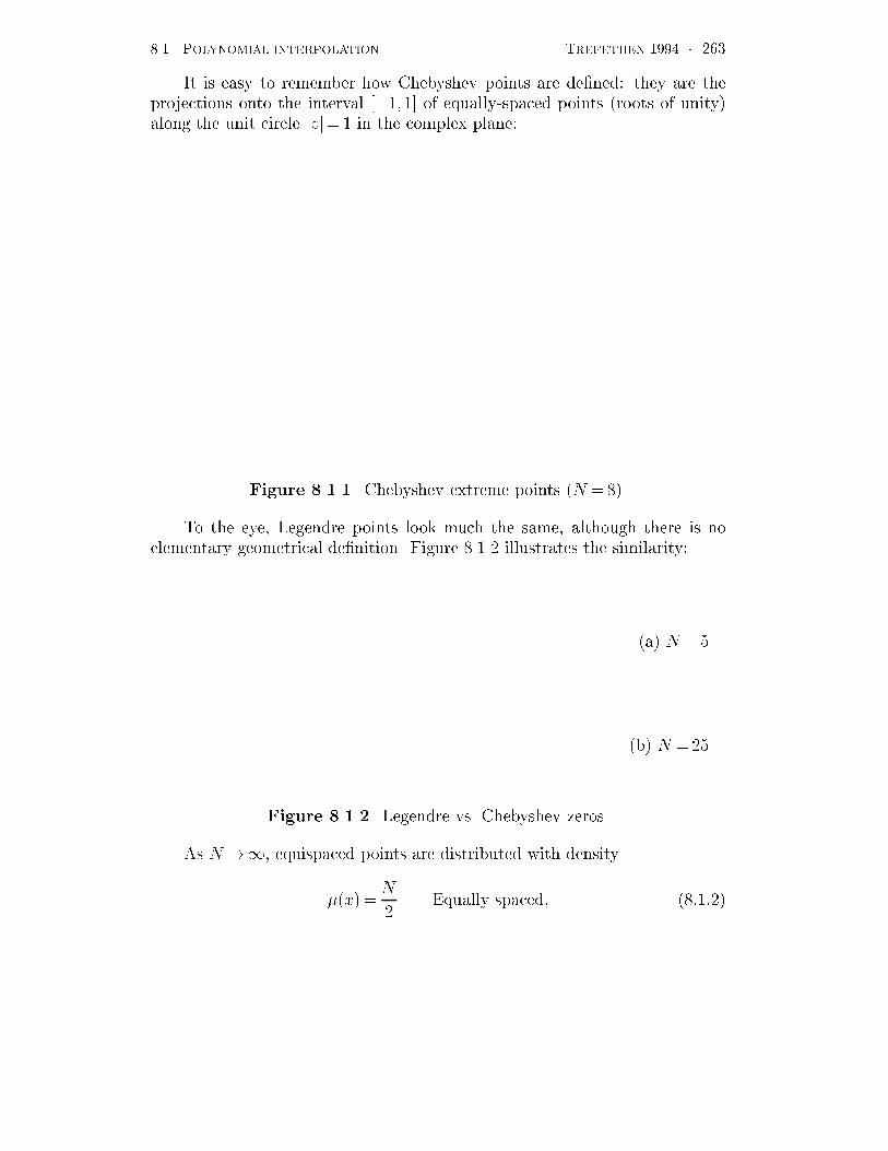
It is easy to remember how Chebyshev points are de�ned� they are theprojections onto the interval �� of equally�spaced points �roots of unity�along the unit circle jzj�� in the complex plane�

Figure �� Chebyshev extreme points �N ��

To the eye� Legendre points look much the same� although there is noelementary geometrical de�nition� Figure �� illustrates the similarity�

�a� N ��

�b� N ��

Figure �� Legendre vs� Chebyshev zeros�

As N�� equispaced points are distributed with density

��x��N

�Equally spaced� ��


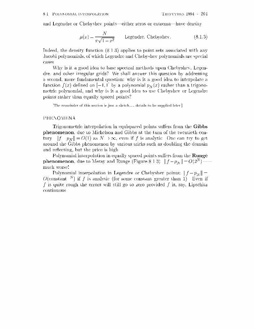
and Legendre or Chebyshev points�either zeros or extrema�have density

��x��N

�p��x�

Legendre� Chebyshev� ��

Indeed� the density function �� applies to point sets associated with anyJacobi polynomials� of which Legendre and Chebyshev polynomials are specialcases�

Why is it a good idea to base spectral methods upon Chebyshev� Legen�dre� and other irregular grids� We shall answer this question by addressinga second� more fundamental question� why is it a good idea to interpolate afunction f�x� de�ned on �� by a polynomial pN �x� rather than a trigono�metric polynomial� and why is it a good idea to use Chebyshev or Legendrepoints rather than equally spaced points�

The remainder of this section is just a sketch� � � details to be supplied later�

PHENOMENA

Trigonometric interpolation in equispaced points su�ers from the Gibbsphenomenon� due to Michelson and Gibbs at the turn of the twentieth cen�tury� kf �pNk�O�� as N �� even if f is analytic� One can try to getaround the Gibbs phenomenon by various tricks such as doubling the domainand re�ecting� but the price is high�

Polynomial interpolation in equally spaced points su�ers from the Rungephenomenon� due to Meray and Runge �Figure �� kf�pNk�O��N��much worse�

Polynomial interpolation in Legendre or Chebyshev points� kf �pNk�O�constant�N � if f is analytic �for some constant greater than �� Even iff is quite rough the errors will still go to zero provided f is� say� Lipschitzcontinuous�


Figure �� The Runge phenomenon�


FIRST EXPLANATION�EQUIPOTENTIAL CURVES

Think of the limiting point distribution ��x�� above� as a charge densitydistribution� a charge at position x is associated with a potential log jz�xj�Look at the equipotential curves of the resulting potential function ��z� �R ��x� log jz�xjdx�

CONVERGENCE OF POLYNOMIAL INTERPOLANTS

Theorem ��

In general� kf �pNk� � as N �� in the largest region bounded by anequipotential curve in which f is analytic� In particular�

For Chebyshev or Legendre points� or any other type of Gauss�Jacobi points�convergence is guaranteed if f is analytic on ��For equally spaced points� convergence is guaranteed if f is analytic in aparticular lens�shaped region containing �� Figure ��

Figure �� Equipotential curves�


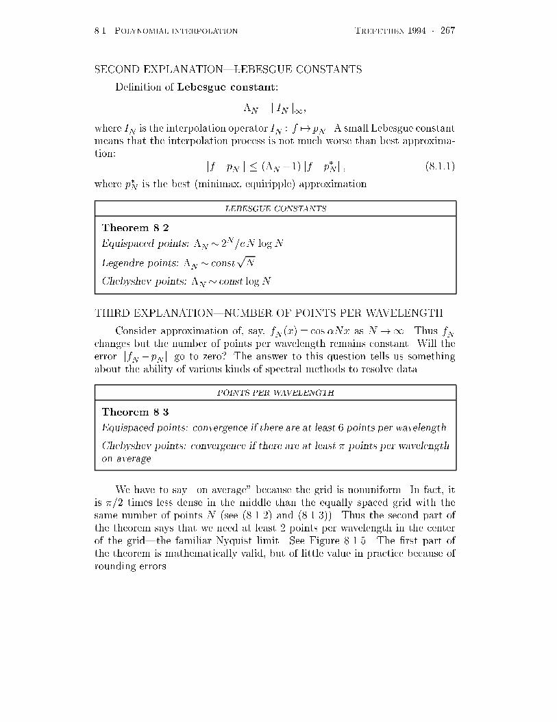
SECOND EXPLANATION�LEBESGUE CONSTANTS

De�nition of Lebesgue constant�

�N � kINk��

where IN is the interpolation operator IN � f �� pN � A small Lebesgue constantmeans that the interpolation process is not much worse than best approxima�tion�

kf�pNk � ��N ��kf�p�Nk� ��

where p�N is the best �minimax� equiripple� approximation�

LEBESGUE CONSTANTS

Theorem ��

Equispaced points� �N �N�eN logN �

Legendre points� �N constpN �

Chebyshev points� �N const logN �

THIRD EXPLANATION�NUMBER OF POINTS PER WAVELENGTH

Consider approximation of� say� fN �x� � cos Nx as N �� Thus fNchanges but the number of points per wavelength remains constant� Will theerror kfN �pNk go to zero� The answer to this question tells us somethingabout the ability of various kinds of spectral methods to resolve data�

POINTS PER WAVELENGTH

Theorem ��

Equispaced points� convergence if there are at least points per wavelength�

Chebyshev points� convergence if there are at least � points per wavelengthon average�

We have to say �on average� because the grid is nonuniform� In fact� itis �� times less dense in the middle than the equally spaced grid with thesame number of points N �see �� and �� Thus the second part ofthe theorem says that we need at least � points per wavelength in the centerof the grid�the familiar Nyquist limit� See Figure �� The �rst part ofthe theorem is mathematically valid� but of little value in practice because ofrounding errors�

�� CHEBYSHEV DIFFERENTIATION MATRICES TREFETHEN ��

�a� Equally spaced points

�b� Chebyshev points

Figure �� Error as a function of N in interpolation of cos Nx�with � hence the number of points per wavelength� held �xed�


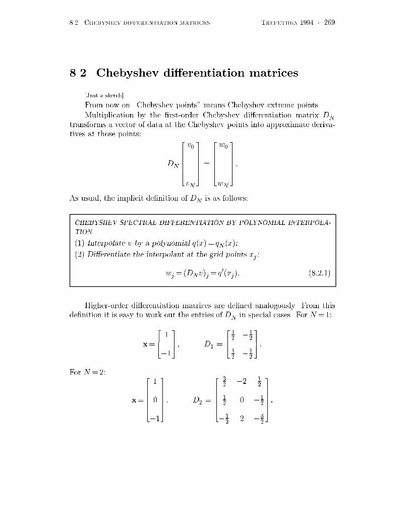
�� Chebyshev di�erentiation matrices

Just a sketch

From now on �Chebyshev points� means Chebyshev extreme points�Multiplication by the �rst�order Chebyshev di�erentiation matrix DN

transforms a vector of data at the Chebyshev points into approximate deriva�tives at those points�

DN

��

v�

��

vN

��

��

w�

��

wN

��

As usual� the implicit de�nition of DN is as follows�

CHEBYSHEV SPECTRAL DIFFERENTIATION BY POLYNOMIAL INTERPOLA�

TION�

�� Interpolate v by a polynomial q�x�� qN �x��

�� Di�erentiate the interpolant at the grid points xj �

wj ��DNv�j � q��xj��

Higher�order di�erentiation matrices are de�ned analogously� From thisde�nition it is easy to work out the entries of DN in special cases� For N ��

x�

��

��

�� D� �

��

�

��

�

��

For N ��

x�

��

�

�

��

�� D� �

��

��

�

��

�

��

�

��


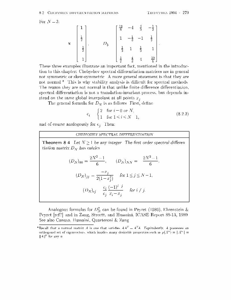
For N ��

x�

��

�

��

��

��

�� D� �

��

��

� ��

� ��

�

��

� ��

� � ��

��

These three examples illustrate an important fact� mentioned in the introduc�tion to this chapter� Chebyshev spectral di�erentiation matrices are in generalnot symmetric or skew�symmetric� A more general statement is that they arenot normal�� This is why stability analysis is di cult for spectral methods�The reason they are not normal is that unlike �nite di�erence di�erentiation�spectral di�erentiation is not a translation�invariant process� but depends in�stead on the same global interpolant at all points xj �

The general formula for DN is as follows� First� de�ne

ci �

�� for i�� or N �

� for �� i�N��

and of course analogously for cj � Then�

CHEBYSHEV SPECTRAL DIFFERENTIATION

Theorem �� Let N � � be any integer� The rst�order spectral di�eren�tiation matrix DN has entries

�DN �� N��

� �DN �NN � ��N��

�

�DN �jj ��xj

��x�j �for �� j�N��

�DN �ij �cicj

��i�jxi�xj

for i � j�

Analogous formulas for D�N can be found in Peyret �� Ehrenstein !

Peyret �ref�� and in Zang� Streett� and Hussaini� ICASE Report � �� See also Canuto� Hussaini� Quarteroni ! Zang�

�Recall that a normal matrix A is one that satis�es AAT � ATA� Equivalently� A possesses anorthogonal set of eigenvectors� which implies many desirable properties such as ��An� � kAnk �kAkn for any n�


A note of caution� DN is rarely used in exactly the form described inTheorem �� for boundary conditions will modify it slightly� and these dependon the problem�

EXERCISES

�� Prove that for any N � DN is nilpotent DnN � for a su�ciently high integer n�

�� CHEBYSHEV DIFFERENTIATION BY THE FFT TREFETHEN ��

�� Chebyshev di�erentiation by the FFT

Polynomial interpolation in Chebyshev points is equivalent to trigonometric interpo�lation in equally spaced points� and hence can be carried out by the FFT� The algorithmdescribed below has the optimal order O�N logN�� but we do not worry about achievingthe optimal constant factor� For more practical discussions� see Appendix B of the book byCanuto� et al�� and also P� N� Swarztrauber� �Symmetric FFTs�� Math� Comp� �� Valuable additional references are the book The Chebyshev Polynomials by Rivlinand Chapter � of P� Henrici� Applied and Computational Complex Analysis ��

Consider three independent variables � � R� x � �� and z � S� where S is thecomplex unit circle fz jzj�g� They are related as follows

z ei�� xRez �

��z�z�� cos ��

which impliesdx

d��sin ��

p��x��

See Figure �� Note that there are two conjugate values z � S for each x� �� andan in�nite number of possible choices of ��

o*

o*

o* ��

�

x

z

z

Figure �� z� x� and ��

�optimal� that is� so far as anyone knows as of ��


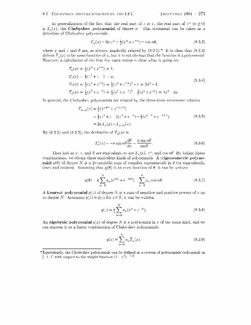
In generalization of the fact that the real part of z is x� the real part of zn �n� ��is Tn�x�� the Chebyshev polynomial of degree n� This statement can be taken as ade�nition of Chebyshev polynomials

Tn�x�Rezn �

��zn�z�n� cos n��

where x and z and � are� as always� implicitly related by �� It is clear that �� de�nes Tn�x� to be some function of x� but it is not obvious that the function is a polynomial�However� a calculation of the �rst few cases makes it clear what is going on

T��x� �

��z��z��

T��x� �

��z��z�� x�

T��x� �

��z��z��

��z��z�� x��

T��x� �

��z��z��

��z��z��

��z��z�� x�� x�

��

In general� the Chebyshev polynomials are related by the three�term recurrence relation

Tn��x� �

��zn��z�n��

�

��z��z��zn�z�n��

��zn��z�n��

�xTn�x��Tn��x��

��

By �� and �� the derivative of Tn�x� is

T �

n�x��n sin n�d�

dxn sin n�

sin��

Thus just as x� z� and � are equivalent� so are Tn�x�� zn� and cos n�� By taking linear

combinations� we obtain three equivalent kinds of polynomials� A trigonometric polyno�

mial q�� of degree N is a ��periodic sum of complex exponentials in � �or equivalently�sines and cosines�� Assuming that q�� is an even function of �� it can be written

q��

�

NXn��

an�ein��e�in��

NXn��

an cos n��

A Laurent polynomial q�z� of degree N is a sum of negative and positive powers of z upto degree N � Assuming q�z� q��z� for z �S� it can be written

q�z� �

�

NXn��

an�zn�z�n��

An algebraic polynomial q�x� of degree N is a polynomial in x of the usual kind� and wecan express it as a linear combination of Chebyshev polynomials

q�x�

NXn��

anTn�x��

�Equivalently� the Chebyshev polynomials can be de�ned as a system of polynomials orthogonal on�� with respect to the weight function ��x��


The use of the same coe�cients an in �� is no accident� for all three of thepolynomials above are identical

q�� q�z� q�x��

where again� x and z and � are implicitly related by �� For this reason we hope to beforgiven the sloppy use of the same letter q in all three cases�

Finally� for any integer N � �� we de�ne regular grids in the three variables as follows

�j j�

N� zj ei�j � xj Rezj

�

��zj�z��j � cos �j ��

for �� j �N � The points fxjg and fzjg were illustrated already in Figure �� And nowwe are ready to state the algorithm for Chebyshev di�erentiation by the FFT�


ALGORITHM FOR CHEBYSHEV DIFFERENTIATION

�� Given data fvjg dened at the Chebyshev points fxjg �� j �N think of the samedata as being dened at the equally spaced points f�jg in ��

�� FFT� Find the coe cients fang of the trigonometric polynomial

q��

NXn��

an cos n� ��

that interpolates fvjg at f�jg�� FFT� Compute the derivative

dq

d��

NXn��

nan sin n��

�� Change variables to obtain the derivative with respect to x�

dq

dxdq

d�

d�

dx

NXn��

nan sin n�

sin �

NXn��

nan sin n�p��x�

� ��

At x�� i�e� �� L�Hopital�s rule gives the special values

dq

dx��

NXn��

��nn�an ��

�� Evaluate the result at the Chebyshev points�

wj dq

dx�xj��

Note that by �� equation �� can be interpreted as a linear combination ofChebyshev polynomials� and by �� equation �� is the corresponding linear com�bination of derivatives�� But of course the algorithmic content of the description aboverelates to the � variable� for in Steps � and � we have performed Fourier spectral di�erenti�ation exactly as in x�� discrete Fourier transform� multiply by i�� inverse discrete Fouriertransform� Only the use of sines and cosines rather than complex exponentials� and of ninstead of �� has disguised the process somewhat�

�or of Chebyshev polynomials Un�x� of the second kind�


EXERCISES

�� Fourier and Chebyshev spectral di�erentiation�

Write four brief� elegant Matlab programs for �rst�order spectral di�erentiation

FDERIVM� CDERIVM construct di�erentiation matrices�

FDERIV� CDERIV di�erentiate via FFT�

In the Fourier case� there are N equally spaced points x�N�� xN�� N even� in

�� and no boundary conditions� In the Chebyshev case� there are N Chebyshev pointsx�� xN in �� N arbitrary�� with a zero boundary condition at x�� The e�ect ofthis boundary condition is that one removes the �rst row and �rst column from DN � leadingto a square matrix of dimension N instead of N��

You do not have to worry about computational e�ciency �such as using an FFT of lengthN rather than �N in the Chebyshev case�� but you are welcome to worry about it if youlike�

Experiment with your programs to make sure they di�erentiate successfully� Of course� thematrices can be used to check the FFT programs�

�a� Turn in a plot showing the function u�x� cos�x�� and its derivative computed byFDERIV� for N �� Discuss the results�

�b� Turn in a plot showing the function u�x� cos��x�� and its derivative computed byCDERIV� again for N �� Discuss the results�

�c� Plot the eigenvalues of DN for Fourier and Chebyshev spectral di�erentiation withN ��

�� STABILITY TREFETHEN ��

�� Stability

This section is not yet written� What follows is a copy of a paper of mine from K�W� Morton and M� J� Baines� eds�� Numerical Methods for Fluid Dynamics III� ClarendonPress� Oxford� ��

Because of stability problems like those described in this paper� more and more atten�tion is currently being devoted to implicit time�stepping methods for spectral computations�The associated linear algebra problems are generally solved by preconditioned matrix iter�ations� sometimes including a multigrid iteration�

This paper was written before I was using the terminology of pseudospectra� I wouldnow summarize Section � of this paper by saying that although the spectrum of the Legendrespectral di�erentiation matrix is of size ��N� asN�� the pseudospectra are of size ��N��for any � �� The connection of pseudospectra with stability of the method of lines wasdiscussed in Sections ��





















�� SOME REVIEW PROBLEMS TREFETHEN ��

�� Some review problems

EXERCISES

�� TRUE or FALSE� Give each answer together with at most two or threesentences of explanation� The best possible explanation is a proof� a counterexample�or the citation of a theorem in the text from which the answer follows� If you can tdo quite that well� try at least to give a convincing reason why the answer you havechosen is the right one� In some cases a well�thought�out sketch will su�ce�

�a� The Fourier transform of f�x�� exp��x�� has compact support�

�b� When you multiply a matrix by a vector on the right� i�e� Ax� the result is alinear combination of the columns of that matrix�

�c� If an ODE initial�value problem with a smooth solution is solved by the fourth�order Adams�Bashforth formula with step size k� and the missing starting valuesv�� v�� v� are obtained by taking Euler steps with some step size k�� then ingeneral we will need k��O�k�� to maintain overall fourth�order accuracy�

�d� If a consistent �nite di�erence model of a well�posed linear initial�value problemviolates the CFL condition� it must be unstable�

�e� If you Fourier transform a function u�L� four times in a row� you end up withu again� times a constant factor�

�f� If the function f�x�� x��x�� is interpolated by a polynomial qN�x�in N equally spaced points of �� then kf�qNk�� as N��

�g� ex�O�xex�� as x��

�h� If a stable �nite�di�erence approximation to ut � ux with real coe�cients hasorder of accuracy �� then the formula must be dissipative�

�i� If

A�

��

��

�

then kAnk�C �n for some constant C ��

�j� If the equation ut � ��A�u is solved by the fourth�order Adams�Moultonformula� where u�x�t� is a ��vector and A is the matrix above� then k�� isa su�ciently small time step to ensure time�stability�

�k� Let ut�uxx on �� with periodic boundary conditions� be solved by Fourierpseudospectral di�erentiation in x coupled with a fourth�order Runge�Kutta

�� SOME REVIEW PROBLEMS TREFETHEN ��

formula in t� For N � �� k � �� is a su�ciently small time step to ensuretime�stability�

�l� The ODE initial�value problem ut � f�u�t� � cos�u� u�� t � �� iswell�posed�

�m� In exact arithmetic and with exact starting values� the numerical approxima�tions computed by the linear multistep formula

vn�� v

n��vn��vn�� k�f

n��fn��fn�

are guaranteed to converge to the unique solution of a well�posed initial�valueproblem in the limit k� ��

�n� If computers did not make rounding errors� we would not need to study stability�

�o� The solution at time t�� to ut�ux�uxx �x�R � initial data u�x�� f�x�� isthe same as what you would get by �rst di�using the data f�x� according to theequation ut�uxx� then translating the result leftward by one unit according tothe equation ut�ux�

�p� The discrete Fourier transform of a three�dimensional periodic set of data on anN�N�N grid can be computed on a serial computer in O�N� logN� operations�

�q� The addition of numerical dissipation may sometimes increase the stability limitof a �nite di�erence formula without a�ecting the order of accuracy�

�r� For a nondissipative semidiscrete �nite�di�erence model �i�e�� discrete space butcontinuous time�� phase velocity as well as group velocity is a well�de�ned quan�tity�

�s� vn�� vn� is a stable left�hand boundary condition for use with the leap frogmodel of ut�ux with k�h��

�t� If a �nite di�erence model of a partial di�erential equation is stable with k�h�� for some �� then it is stable with k�h�� for any ��

�u� To solve the system of equations that results from a standard second�orderdiscretization of Laplace s equation on an N�N�N grid in three dimensionsby the obvious method of banded Gaussian elimination� without any clevertricks� requires ��N�� operations on a serial computer�

�v� If u�x�t� is a solution to ut � iuxx for x�R � then the ��norm ku�� t�k is inde�pendent of t�

�w� In a method of lines discretization of a well�posed linear IVP� having the ap�propriate eigenvalues �t in the appropriate stability region is su�cient but notnecessary for Lax�stability�

�x� Suppose a signal that s band�limited to frequencies in the range ��kHz� ��kHz�is sampled �� times a second� i�e�� fast enough to resolve frequencies in therange ��kHz��kHz�� Then although some aliasing will occur� the informationin the range ��kHz��kHz� remains uncorrupted�

�� TWO FINAL PROBLEMS TREFETHEN ��

�� Two �nal problems

EXERCISES

�� Equipotential curves� Write a short and elegant Matlab program to plotequipotential curves in the plane corresponding to a vector of point charges �inter�polation points� x�� xN � Your program should simply sample N��P log jz�xj jon a grid� then produce a contour plot of the result� �See meshdom and contour��Turn in beautiful plots corresponding to �a� � equispaced points� �b� � Chebyshevpoints� �c� �� equispaced points� �d� �� Chebyshev points� By all means play aroundwith �D graphics� convergence and divergence of associated interpolation processes�or other amusements if you re in the mood�

�� Fun with Chebyshev spectral methods� The starting point of this problemis the Chebyshev di�erentiation matrix of Exercise �� It will be easiest to usea program like CDERIVM from that exercise� which works with an explicit matrixrather than the FFT� Be careful with boundary conditions� you will want to squarethe �N��N�� matrix �rst before stripping o� any rows or columns�

�a� Poisson equation in �D� The function u�x� � ��x��ex satis�es u�� andhas second derivative u��x� ��x�x��ex� Thus it is the solution to theboundary value problem

uxx��x�x��ex� x� �� u��

Write a little Matlab program to solve �� by a Chebyshev spectral method andproduce a plot of the computed discrete solution values �N�� discrete points in�� superimposed upon exact solution �a curve�� Turn in the plot for N ��and a table of the errors ucomputed��uexact�� for N �� What can yousay about the rate of convergence�

�b� Poisson equation in D� Similarly� the function u�x�y�� x��y��cos�x�y�is the solution to the boundary value problem

uxx�uyy� �sorry� illegible�� x�y� �� u�x��u��y��

Write a Matlab program to solve �� by a Chebyshev spectral method involvinga grid of �N � �� interior points� You may �nd that the Matlab commandKRON comes in handy for this purpose� You don t have to produce a plot ofthe computed solution� but do turn in a table of ucomputed��uexact�� forN �� How does the rate of convergence look�

�c� Heat equation in �D� Back to �D now� Suppose you have the problem

ut�uxx� u�� t�� u�x�� x��ex� ��

�� TWO FINAL PROBLEMS TREFETHEN ��

At what time tc does maxx��u�x�t� �rst fall below �� Figure out the answerto at least � digits of relative precision� Then describe what you would do if Iasked for �� digits�

Documents

C HAPTER T REFETHEN - University of Oxford · C HAPTER T REFETHEN Chapter Cheb yshev sp ectral metho ds P olynomial in terp olation Cheb yshev dieren tiation matrices Cheb yshev dieren