Calculating Mass of Higgs Boson, and Complex (Imaginary?) Higgs Boson

Mass Changed to Real Mass in Electro-Weak Era

ANDREW WALCOTT BECKWITH

Physics department

Chongqing University College of Physics, Chongqing University Huxi Campus

No. 55 Daxuechen Nanlu, Shapingba District, Chongqing 401331

which is in Chinese:重庆市沙坪坝区大学城南路55号重庆大学虎溪校区

People’s Republic of China

Rwill9955b@gmail.com Abstract

We obtain a polynomial based iterative solution for early universe creation of the Higgs boson mass, using a

polynomial 4 3 2 1

1 2 3 4 5 0h h h hA m A m A m A m A with the coefficients for iA derived through integral

formulations with 1

hm the mass of a Higgs boson, and the construction of the coefficients derived as of the iA

using a potential system, for the Higgs, largely similar to the Peskin and Schroeder quantum field theoretic treatment

for a Higgs potential. Afterwards, we examine if mass may have complex number and possibly imaginary values,

with attendant description of consequences in the electroweak regime of space-time. We end with a description of

Imaginary mass becoming Real in Electroweak, with resultant consequences for DM discussed in the last section

with explicit construction of space-time bubbles nucleated due to imaginary mass of Higgs becoming real, as a

contributing source of GW radiation in Electroweak era

I. Introduction We first of all review what was done in a prior document, as given in Appendix A, as far as finding roots

of a fourth order polynomial and the question of Higgs mass. We begin with a traditional Higgs mass

calculation, much of which is taken from Peskin and Schroeder (1995). [1],[2] similar to Halzen

and Martin [1],[3] as well as Kleinert [1],[4], whereas we will use material from Maggiore [5] as

to identify a protocol for a fourth order polynomial in Higgs Mass, while assuming a Higgs style

potential as given in [1],[2] which is also discussed in [3] and[4] in a more general fashion, to

come up with a procedure as to analyze hm mass, After this, we will calculate the range of

integration given in Eq. (1) and Eq. (2) below. Which will be used to evaluate Eq. (1) below.

Note we do not agree to the [6] [20] interpretation, but the issues it brings forward can be

addressed as to isolating out the mass of a Higgs particle hm as a solution to the polynomial

equation. Which comes about due to the potential system given in Appendix A.

4 3 2 1

1 2 3 4 5 0h h h hAm A m A m A m A (1)

Note that we are doing is to walk this to Eq. (15) of our text, in which we urge the readers to go

to Appendix B ,which has the coefficients of Eq. (1) in what is Eq. B(3). For the different

coefficients for iA We then go next to define how we evaluated the coefficients in Eq. B(3) of

Appendix B. In addition, when we use these results, from Appendix A and Appendix B, we

will set the stage for real and imaginary Higgs mass, which will lead to accessing, say at the start

of the electroweak era the details given in Appendix C, as to the formation of Singlet Dark

matter. We close with a proof of how minimum uncertainty principle sets up Appendix D, for

the formation of a magnetic field, which is concurrent with the production of Gravity due to the

collision of bubbles of space time, and also due to the variability of the space-time conditions for

DM singlet production. We conclude with a calculation as to the radii of the bubble of space-

time for which there would be a imaginary to real Higgs mass formation in the Electroweak era.

II. Numerical procedure used to give first order integration values in Eq.

B(3) of Appendix B

Initially we could use the following Integral for Eq. (1) and Eq. B(3) of appendix B, along the lines of

1

1 12

1

1

1

1

2

11 11

expexp 1

expexp

exp log ......1! 2 2!

B rdr r B r B r

B

B rdr B r

B

B rB rdr r B r r

(2)

These in themselves do not give a physical feel as to the dynamics of the situation as well as the

change from Imaginary to Real values in the Electroweak era, which will lead to new physics

later on. Due to the smallness of the value 2

plancklr

t E

which will be evaluated, the

following is a default choice , i.e.. Gauss quadrature [7],[8],9]

0

0

4

0 0

1 3 1 3( )

2 2 6 2 6

r r

r

rf r dr f r r f r r r

(3)

In this case, the values of function f will be dependent upon the details of what is chosen for the

different integrands in the five integrals given in Eq. (7), but due to the smallness of

2

plancklr

t E

, we claim that this will put a premium upon the evaluation of a suitable E

value, and we will next, in order to address this, detail procedures as to isolating optimal E

values in order to ascertain, optimal strategies for implementing Eq.(2) strategies on the integrals

given in Eq. (7) This means, above all, accessing Appendix A below, and then using that

information as a tie into section III below.

This means, above all, accessing Appendix A below, and then using that information as a tie

into section III below. Appendix B, will give a condensed version of the ideas used to form the

Polynomial in Eq. (1).

III. Optimal E strategies, possibly from astrophysical data, We will look at what is given in [10]as to an elementary Fluctuation – Dissipation theorem given in Pages

325-327, i.e. first of all we define a spectral density type of derivation for an average energy, given by, for

a Bose system in a heat bath, of quantum oscillators, which becomes

0

0 0

/ 21Bmean k T temperature

Ee

(4)

Assume that T, temperature is of the order of over 100 GeV, and that we will also have

frequency 0 , for the background as to the creation of particles in the electroweak era. i.e. our

estimate is, then that we will be able to assert, then that with temperature of a very large

magnitude, and with frequency ~ 1/ (time for initiation of electro weak regime) that if we have

0

0

0 0

/

0

0 0

/

21

~2 1

B

B

mean k T temperature

B

mean k T temperature

Ee

k T temperature Electro weak

E E very bige

(5)

This would push down the magnitude of r

0

/

0

/

1

2

1

/

2

2

B

Btime for initiation of electr

k T temperatureplanck planck

k T temperao weak regi tureplan k

ec

m

time for initiation of electro

l ler

t E

weak regim

t

t e

le

(6)

IV. Examining issues as to root finders and Eq. (1) Doing this means we will be considering an optimal set of procedures so as to find a numerical protocol

as to solve for a fourth order polynomial for iteration of mass of hm . If we wish to solve for a fourth

order equation and we are examining to obtain real values for hm one of the very few papers giving the

Cardano solution is sourced here, i.e. [11], and then one also look at [12],[13],[14], [15], for the idea of

the Descartes rule of signs. In other words, if Eq. (1) and its inputs are defined properly one has the

probability one is looking at a real and complex part of a solution to hm

V. Ground zero, what if we obtain hm with real and complex coefficients as

far as a solution to Eq. (1) above? Beyer, [16] has standard root finding procedures for Eq (1) on page 12. Note that in doing it, we

STILL have to obtain the cubic solution to the equation, given below, namely as given by [16],

page nine, we need to use the standard cubic root finders to solve for the rescaled cubit

polynomial.

3 2 2 2( ) 4 0y by ac bd y a d bd c (7)

Where

3 52 4

1 1 1 1

, , ,A AA A

a b c dA A A A

(8)

And of course we will be requiring that in Eq.(11) below, is that to solve for Eq. (1) in full

generality, we will almost certainly be observing complex valued solutions to hm . If we solve for

hm and obtain complex valued solutions to the Higgs mass, as obtained this way, we then have some

fundamental questions to answer. Before we do that, let us review below, in Eq. (10) the full

generality of our answer. It is to put it very specifically, a huge mess. Why would we do this or

want to do it?

VI. Implications if a mass for the Higgs has real and complex components,

i.e. imaginary mass has Tachyon mass properties (Faster than light ). As

cited from Baez, reference [17].

What we can expect if the Higgs, say has both real and imaginary mass, and we should note that Baez

says that if the mass of a particle is purely imaginary that, in [17], this means faster than light

travel. We suppose from what we know of real valued Higgs physics, as to what is given in the

middle to latter part of the Electroweak era [18], that [2] ,[3], to [4] actually hold up very well. According to Baez, [17], we then have if the mass is purely imaginary, a situation where one has particles

which travel faster than the speed of light, i.e. the Tachyon. What we are supposing, taking a line from

[17] is a situation in which then at least part of the mass will contribute to faster than light ‘travel’. This is

also discussed on page 16 and 17 of [18] , albeit as a supposed fault of prior to present day String theory

models.

PrRe Im Im

&

' tan (inf )

Re Im Re

&

tan

h h h hior To Electroweak era

h h h hElectroweak era to today

m m i m i m

Quantum en glement ormation transfer

m m i m m

S dard Model Higgs mass formation properties

(9)

Getting a description of this modeling would require extensive numerical and analytical

treatment of Eq. (1), which we see in Eq. (10) below, with the result that we have the following

decomposition of the Eq. (1) if we wish to have a generalized complex Higgs Boson mass. Keep

in mind that we put a restraint in, in order to have a comparatively simple value, but this is done

in such a way as NOT to appeal to an inflection point for the solution to the resulting third order

equation which is used.

Our next iteration takes the inflection points of our derived third order polynomial in terms of the

Higgs Boson mass, but we start off with a solution without appealing to the inflection points of

this iterative system for solving for the mass of a Higgs Boson at the start of the expansion of the

universe. First, let us start off assuming no inflection point for the third order polynomial in

Higgs mass [1],[16]

4 3 2 1

1 2 3 4 5

4 3 2 13 52 4

1 1 1 1

4 3 2

1 3 52 4

1 1 1 1

3 2 2 2

0

0

0

, , , ,

,

( ) 4 0

/ 4 / 2 / 2

h h h h

h h h h

h

A m A m A m A m A

A AA Am m m m

A A A A

is linkable to

x ax bx cx d

A AA Ax m a b c d

A A A A

Then to

y by ac bd y a d bd c

x a R D

or

x

2

/ 4 / 2 / 2

4

a R E

where

aR b y

(10)

Here, we have two cases, depending upon the value of R, and NOT assuming inflection points

for the Third order equation.

2 32

2 32

22 2

22 2

0

3 4 82

4 4

3 4 82

4 4

0

32 2 4

4

32 2 4

4

If R

a ab c aD R b

R

a ab c aE R b

R

If R

aD b y d

aE b y d

(11)

We then read off the following integrals, i.e. Go to Eq. (2) of our document. Also we make the

following approximations, In doing so we set up a complex field interpolation for the mass, m, of

the Higgs mass and we do it with the following assumptions. Pick the following reduced

equation for the cubic, and we obtain, from CRC, page 12 that[16]

3

1 2

2

1 2 1

2

2 1 1 2 3

1

2

2 2

3

0

/ 3

12 9 27

27

( )

4

Then

z a z a

a a a

a a a a a

a b

a ac bd

a a d bd c

(12)

Which allows us to write z as having the following solution

2 23 3

2 2 1 2 2 13 3

3

1

,2 2 27 2 2 27

/ 3

; / 2 / 2 3

; / 2 / 2 3

a b

a b a b a b

a b a b

a a a a a aA B

y z a

z A B A B A B

A B A B

(13)

Then we make the following assumption, namely if we want to have a complex Higgs mass we

could write the following assumption. (NOT assuming a third order equation inflection

point! )

2 3

2 1

2/32 332

22/3 3 32 2

2 27

2 2 cos sin2 3 3

1 27cos sin 2

3 3 3 4

a aSet

az i a

y i a a

(14)

This value of y, will then be put into R above. Having said this, we will review a simpler

procedure and limiting cases for how one could achieve an (almost ) imaginary mass value.

XII. Problem of what happens if we have a complex mass value, in terms of

physics for Higgs, and what happens if the mass goes to real values? I.e. what we have in that case, is that we can look at when we will have a real mass. I.e. the key

is to examine where Eq. (10) will have an inflection point and from there to extrapolate to the

real valued version of this problem. I.e. our supposition is that we will go to the inflection point

of Eq. (11), come up with a value of y, so then that after, first calculation of R, then obtaining y,

and then obtaining x, effectively then obtaining the mass value of the Higgs, real valued for the

solution of Eq. (1) above, And then we obtain the following real value for the Higgs boson,

namely

2 322

1

3 52 4

1 1 1 1

22

3 4 82

2 4 44

, , ,

2 13

4 3 3

h

A R a ab c am E R b

RA

A AA Aa b c d

A A A A

a bR b ac bd

(15)

This takes into account the inflection point of Eq. (10), which is treating both parts of Eq.(15)

as real valued, with the resultant value of hm > 0 but real valued for suitably chosen values of the

values of Eq.(2) put in. What this is saying, i.e. the complex value of hm is for the Pre Planckian regime

of space-time whereas we should use Eq.(15) to come up with Mass‎:‎‎125.09±0.21 (stat.)±0.11 (syst.) GeV/c2 .and a Mean lifetime‎:‎‎1.56×10−22 s (predicted) Now, how could we ascertain an imaginary mass for the Higgs Boson? First of all would be

setting R = 0. The other would be in having an infinitesimal value for 2

1

Aa

A First

2

22 22

1

22 22

1

2 2

2

32 2 4

44

32 2 4

44

2 2 4

13

3

h

A

A am E b y d

A

A aE b y d

A

b y d

when y b b ac bd

(16)

We further simplify the mass of the Higgs Boson by writing Eq. ( 16) as stated by Eq. (17) as

2

2 2

3 52 4

1 1 1 1

22

12 2 3 4

3

, , ,

2 13 0

4 3 3

hm b b b bd d

A AA Aa b c d

A A A A

and

a bR b ac bd

(17)

We can justify both Eq. (17) and Eq.(16) in terms of a sliding scale as far as what we put in for

r in the integrals specified for Eq. (2) . Our supposition is that the dividing line between Eq.

(16) and Eq. (17) is due to how we vary r with a small value of r commensurate with Pre

Planckian values for the Higgs mass, i.e. the Higgs mass would be largely then imaginary, which

would be due to R = 0, and also 2A

, leading to Eq.(17) to be dominated by imaginary

mass. Whereas for r with a larger value, we would be then tending toward Eq. (15) which

would be centered upon Eq.(3). I.e. which is influenced by r

XIII. What we are leading up to, is the change from Eq. (17) imaginary

value, to Eq. (15) real value corresponds to when bubbles, in space-time, form

in the Electro-weak regime. Here is why. What we are going to do is to claim that when we use the Duerrer bubble nucleation with the

space time bubbles commencing in formation when there was a transfer from largely imaginary

Higgs Boson mass, to real Higgs Boson mass, in the Electroweak era. The way to start this is to

look at a way to form mass, from the transfer from Imaginary to Real space-times, and to do it

with respect to the Electroweak regime. From [19] we isolated the way to have an equivalent mass,

based upon a nonstandard way to illustrate a basic cosmology as given by

Quote: pages 38-39 of [19]

We begin with a non standard representation of mass from Plebasnki and Krasiniski [20]which affirms

the likelihood of the synthesis of mass, if and when the radii of a universe, due to a metric is non zero. I.e.

[20] , page 295, and page 296

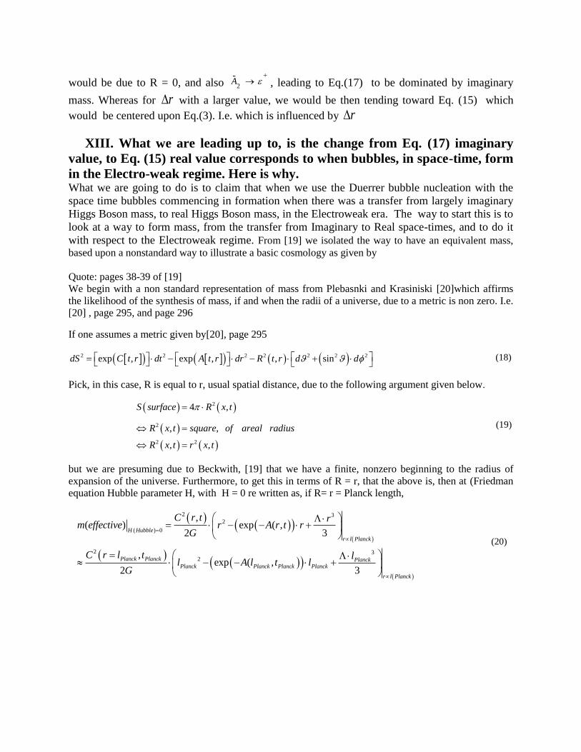
If one assumes a metric given by[20], page 295

2 2 2 2 2 2 2exp , exp , , sindS C t r dt A t r dr R t r d d (18)

Pick, in this case, R is equal to r, usual spatial distance, due to the following argument given below.

2

2

2 2

4 ,

, ,

, ,

S surface R x t

R x t square of areal radius

R x t r x t

(19)

but we are presuming due to Beckwith, [19] that we have a finite, nonzero beginning to the radius of

expansion of the universe. Furthermore, to get this in terms of R = r, that the above is, then at (Friedman

equation Hubble parameter H, with H = 0 re written as, if R= r = Planck length,

2 32

( ) 0

2 32

,( ) exp ( ,

2 3

,exp ( ,

2 3

H Hubble

r l Planck

Planck Planck PlanckPlanck Planck Planck Planck

r l Planck

C r t rm effective r A r t r

G

C r l t ll A l t l

G

(20)

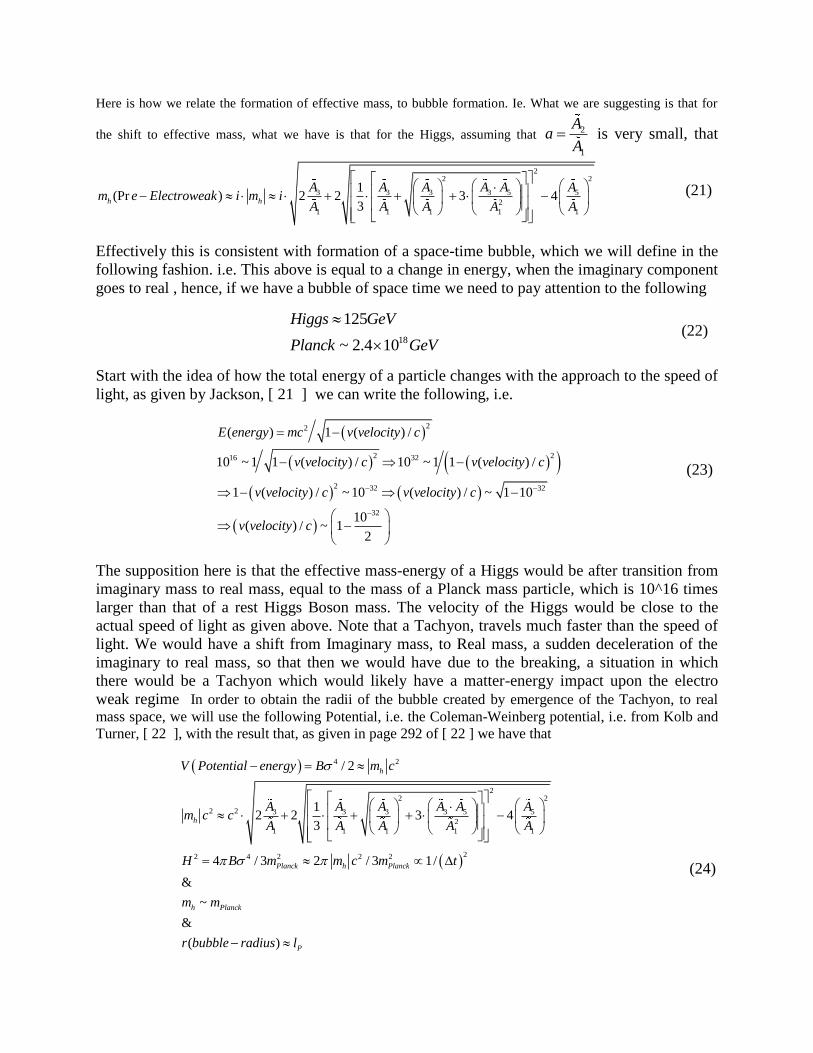
Here is how we relate the formation of effective mass, to bubble formation. Ie. What we are suggesting is that for

the shift to effective mass, what we have is that for the Higgs, assuming that 2

1

Aa

A is very small, that

22 2

3 3 3 3 5 5

2

1 1 1 1 1

1(Pr ) 2 2 3 4

3h h

A A A A A Am e Electroweak i m i

A A A A A

(21)

Effectively this is consistent with formation of a space-time bubble, which we will define in the

following fashion. i.e. This above is equal to a change in energy, when the imaginary component

goes to real , hence, if we have a bubble of space time we need to pay attention to the following

18

125

~ 2.4 10

Higgs GeV

Planck GeV

(22)

Start with the idea of how the total energy of a particle changes with the approach to the speed of

light, as given by Jackson, [ 21 ] we can write the following, i.e.

22

2 216 32

2 32 32

32

( ) 1 ( ) /

10 ~ 1 1 ( ) / 10 ~ 1 1 ( ) /

1 ( ) / ~ 10 ( ) / ~ 1 10

10( ) / ~ 1

2

E energy mc v velocity c

v velocity c v velocity c

v velocity c v velocity c

v velocity c

(23)

The supposition here is that the effective mass-energy of a Higgs would be after transition from

imaginary mass to real mass, equal to the mass of a Planck mass particle, which is 10^16 times

larger than that of a rest Higgs Boson mass. The velocity of the Higgs would be close to the

actual speed of light as given above. Note that a Tachyon, travels much faster than the speed of

light. We would have a shift from Imaginary mass, to Real mass, a sudden deceleration of the

imaginary to real mass, so that then we would have due to the breaking, a situation in which

there would be a Tachyon which would likely have a matter-energy impact upon the electro

weak regime In order to obtain the radii of the bubble created by emergence of the Tachyon, to real

mass space, we will use the following Potential, i.e. the Coleman-Weinberg potential, i.e. from Kolb and

Turner, [ 22 ], with the result that, as given in page 292 of [ 22 ] we have that

4 2

22 2

2 2 3 3 3 3 5 5

2

1 1 1 1 1

22 4 2 2 2

/ 2

12 2 3 4

3

4 / 3 2 / 3 1/

&

~

&

( )

h

h

Planck h Planck

h Planck

P

V Potential energy B m c

A A A A A Am c c

A A A A A

H B m m c m t

m m

r bubble radius l

(24)

We then would have that there would be Planck sized bubbles of space, time for suddenly

appearing in the Electroweak regime of space time Higgs boson mass sized nucleation, which

would then be inclined to ‘bounce’ off each other. The transition of imaginary to real mass

values, would lead to then the idea of entanglement which is discussed below

Quote, [19] page 39

We claim that this effective mass should be put into the following wave function at the boundaries of the

H = 0 causal boundary, as outlined by Beckwith, in [23]. Then we make the following approximation at

the H = 0 causal boundary, for the entangled wavefunction for Faster than light transmission of ‘quantum

information’, i.e.

tan

2 2 2 2 2 2 2 2

Pr Pr

0 0

2 2 2 2 2 2 2 2

Pr Pr

0 0

n n1 1 11 1

3! 2 3! 28

n n1 1 11 1

3! 2 3! 28

En gled

A ior B esent

A esent B ior

r r

mE mE

r r

mE mE

(25)

End of quote

What we are suggesting is that we may have something very similar as to the formation of mass problem,

for a Higgs, with the positions r (prior) referring to prior universe positions, and r(present) referring to

positions as of about the formation(start) of the electro weak era. The indices (A) and (B) refer to

information states in the prior to present universe which would be relatively instantaneously transferred

from the prior to the present universe. I.e. the position r(present) would be about at the start of the

electroweak era in the present universe, i.e. an ‘imaginary’ mass corresponding to ‘information’ packet

which is almost instantaneously transferred. Our supposition is that imaginary mass, not being measurable

in our space-time, would be in its transfer from a present to a prior universe, similar in the entanglement

information exchange as referenced in [1], [24], [25], [26].

This is a detail which has to be worked out. The numbers n(A) and n(B) in this case would refer to

specifically numbered states of matter – energy packets whose information would be exchanged almost

instantaneously from a prior to a present universe. In this case, our supposition is that any would be

imaginary mass, going in between the prior to present universe, would probably be unmeasurable, until

they went to being a real valued traditional mass value.

. Our next goal will be to see if there is any linkage of this topic with that as to gravity waves and

gravitation.

XII. Does our formulation of Higgs bosons with imaginary mass, initially

(information transfer?) help to explain initial gravitational wave

generation?

So far, we have discussed the formation of a Higgs mass, with, prior to and then up to the start of the

Electro weak era having at least some imaginary mass component.

To rephrase our question, what would happen if the mass went from an unmeasurable by physics

instruments imaginary value to real value, say as in the middle of the Electroweak transformation?, i.e. to

see what we are referring to, we go to [27] where massive gravitons are conflated with Dark energy, and

also we have that [26] has explicit linkage of early universe graviton states, as generated by information

transfer from prior to present universe conditions as seen in the counterpart to (49) in [19], which we have

already cited. Our supposition is that the emergence of Higgs mass due to the following transformation

created local space-time turbulence, hence thereby generation of GW, and what we suppose are gravitons.

So we will make the following linkage between a change from imaginary (Higgs boson mass), to real

(Higgs boson mass), and then the generation of GW, from what would be a phase transition induced in the

Electro-weak era, as we go directly to real valued Higgs boson mass, from an earlier imaginary valued

Higgs boson mass. This would induce turbulence, in local space time which would also then induce GW,

and by default, massive gravitons.

This is an extension of discussions given in [1], [28], [29], [30]

Chiara Caprinia, Ruth Durrer and G´eraldine Servant [1], [28] state specifically that

Quote: page 2 of [28], and also part of [1] we have

Although the first GW detections will come from astrophysical processes, such as merging of

black holes, another mission of GW astronomy will be to search for a stochastic background of

GWs of primordial origin. An important mechanism for generating such a stochastic GW

background is a relativistic first-order phase transition. In a first-order phase transition, bubbles

are nucleated, rapidly expand and collide. The free energy contained in the original vacuum is

released and converted into thermal energy and kinetic energy of the bubble walls and the

surrounding fluid. Most of the gravitational radiation comes from the final phase of the

transition, from many-bubble collisions and the subsequent MHD turbulent cascades. The

associated GW spectrum encodes information on the temperature of the universe T∗ at which the

waves were emitted as well as on the strength of the transition. The characteristic frequency of

the waves corresponds to the physics that produces them

End of quote

Note that in [1], [28] , we have the following approximations given in page 36 of that document ,

in [28] to the effect that

~ 8

1/

1/ GW

h GT

h Amplitude of GW producing Perturbation

Characteristic time which GW producing Perturbation occurs

Gravitational wave frequency

T Energy momentum tensor of source for crea

( ) 1/ 8GW

tion of GW

GW energy density G T

(26)

In [21] we estimated a relic GW frequency of the order of 1/Planck length, i.e ~10^35 GHz, or

higher, i.e. very high, at the start of the Electroweak regime, or just before at the beginning of

Planckian physics.What we will be doing later will be to make an argument as to what T should

be following an emergence of imaginary (initially) Higgs bosons, transferred to real Higgs

bosons, in the middle of the Electroweak era. We submit that the emergence from imaginary to

real space time of such Higgs bosons, would precipitate the creation of the bubbles in space time

which would subsequently collide, thereby generating gravitational waves and turbulence, and

we will briefly state what this may presage as far as Dark Matter.

XIII. Starting off with a setting of stationary Initial states, as given by an

example from Merzbacher, which we cite and quote. Leading to

imaginary to real Higgs mass transformation creating turbulence which

would break up the initial stable state. And be when DM forms.

First of all, we will review what is mean by a wave function which reflects minimizing uncertainty, in

Quantum mechanics. This is given by Merzbacher [ 31 ] in the following argument which will be then

adopted and modified as to issues in DM production as we call it.

Merzbacher [ 31 ] in page 161 of his book gave a simple Schrodinger Equation, one dimension for a

minimum uncertainty state as having the form

2

21/4

2

2

2

2 exp4

/ 2

x

x

d ip x x

i dx x

x x i p xx

x

x p

(27)

As Merzbacher relates, in [ 31 ], this is for, spatially, a situation for which there is a specified

linkage as to change in position to a directly correlated momentum variance. With the result that

the wave function has both Gaussian and Plane wave characteristics superimposed upon each

other directly. We can state that then, if we go to the problem of representation of a matter wave,

in the regime of Planckian space-time that the above is similar to , if we take it literally, of the

following wavefunction approximation

21/4

2

2~ 2 exp

24Planckian space time

x x ix

x

(28)

In other words, aside from a phase factor, of 0.877582562 0.47exp 942( / 2) 55~ 39 i i , this

wavefunction argument so parlayed, would be a way of identification of how we could write

21/4

2

20.877582562 0.47942~ 2 e5 x39 p5

4Planckian space time

x xxi

x

(29)

I.e. a complex valued wave functional, at the edge of the uncertainty principle, with real and

Complex magnitude, which is in line with treating exp(i/2) as a phase factor, whereas the factor

2

2exp

4

x x

x

(30)

should be thought of as a Gaussian wave function type development. I.e. this is in tandem with

our supposition as to having a tie in with another result from Merzbacher, [ 31 ] to the effect that

if we have again, as a start, a Harmonic oscillation, with initial conditions of( see page 165 of

[ 31 ] )

2

2

, 1/42

2

~ ,0 ~ exp2

, exp

&

cossin sin 2

2 2 4

&

,

Planckian space time Initial conditions HO

a x x

later conditions HO

later conditions HO

x ax N

x t N

x a ti t ax t a t

x t os

1/4

2 2, 1/ 4 0.877582562 0.4794255, ~ 3 2

29

cillates without change of shape

with

a x x iN x

(31)

This is important on several levels. It suggests that if there is a minimum Heisenberg Uncertainty

principle as to initial conditions for a wavefunction at the start of the inflationary era, obeying initial

imperatives similar to the SHO, that according to Eq. (31) based upon page 165 of Merzbacher, [31] there

would be NO variation as to the spatial component as to the absolute magnitude form of the shape of the

initial wavefunction of a system with minimum uncertainty.

We have postulated minimum uncertainty, as far as the boundary between the Pre Planckian physics, to

Planckian physics regime, and if space is acting, initially spatially in a one dimensional type of spatial

action, this means that IF we have some form of harmonic motion, initially, if the Initial conditions are in

line with Eq. (30) that there would be NO spatial variation in time, at least before the formal onset of

inflation. Hence, this also requires a Schrodinger type argument with initial conditions being congruent as

to Eq. (27) above, with / 2x p being approximately implying the formation of Eq. (30)

above. And that at the boundary just after Pre-Planckian-to Planckian physics length ( just

before Electro-weak) regime, giving credence to the idea of states of matter which would be

changing from perhaps an imaginary mass value, to real value along the lines suggested by Eq.

(21) and Eq. (24) above.

What would cause a violation of this zone of would be near spatial non variability ? In a

word, the shift from Imaginary to Real mass as far as the HIGGS boson . Ie. Up to the

point this would happens, we would have due to the reasoning in Eq. (31) a pre Planckian

regime of space-time stability which would be broken apart by the shift from Imaginary to

Real Higgs mass !

Having initial wavefunction conditions in a regime of space-time given by Eq. (31) right at the

junction of where we have Higgs mass change from imaginary, to real, along the lines of Eq.(9)

above will lead to conditions for when we can discuss the potential effects upon DM. i.e. see

Appendix C, for what we have to say about the Singlet model of DM. Whereas if we wish to

use the idea of Gravitational wave generation we can avail ourselves to the matter of reference

[ 28 ] given which has a crucial quote as to a regime of space – time turbulence. I.e. see

Appendix D, which we quote the last two equations. One for a current, and one for a B field. It

is our contention that the B field is commensurate with the formation of non imaginary mass, in

the Electroweak regime. As a result of mass formation, which is what the Higgs is all about.

Quote

(From Appendix D), we would have a current we will call

0

0

3 11~ 1

2 8I j

G t t G V

(32)

(Then our net magnetic field, is to first approximation given by use of linkage of E and B fields given by

Griffiths [32] as resulting in)

0

1/42

0

0 0

( )

3 11~ 1 1

2 8

netB magnetic field B

G t t G V

(33)

End of quote

Our formation of Dark matter, will ALSO avail ourselves of a generation of strong initial

magnetic fields, in the vicinity of the transition between complex (possibly pure imaginary)

Higgs boson mass, to real Higgs mass, partly due to the generation of space-time bubbles to

match the aims of Eq. C(8) of Appendix C. I.e. we state that eq. (32) and Eq. (33) which are

from Appendix D form right in the aftermath of the range of applicability of Eq. C(8) of

appendix C, below.

I.e. to put a finer point on it, we have the aftermath of the breakdown of the relations referred to in Eq.

(31), i.e. the end of stationary pattern for an initial wavefunction, absolute value, with no spatial variation

due to a minimum uncertainty principle.

Once that quasi stationary condition of Eq. (31) breaks down, even if we have harmonic conditional

oscillatory behavior, due to non minimum uncertainty relations commencing as given, we can have Eq.

(32) and Eq. (33), as well as perhaps the generation of Gravitational waves.

We after stating this will make our concluding remarks as far as how to tie in the production of B fields

with Higgs bosons becoming real valued, and that also with GW production, in our conclusion

XIV. Conclusion: Tie in of our supposition about Imaginary to real mass for

Higgs Boson, and the current + B field of Eq. (32) and Eq.(33)

First of all, we will try to tie in our Imaginary to real mass value of the Higgs Boson, to a current, similar

to Eq. (32). To do this, we will use a typical definition of what Soper called a mass current [ 33 ] in order

to make our point

Here, use what Soper called the current, namely on page 38, the number of ‘atoms’ per unit volume. In

our example, replace the caveat of ‘atoms’ with real mass Higgs Bosons

In [ 33 ], page 38, Soper writes

3 (0) ( , )d x J t x Number of atoms (34)

In our supposition, we will replace the term , ‘Number of Atoms’ with number of Higgs bosons,

and then we have that

0

0

0

1/42

0

0 0

1/42

0

0

3 11~ 1

2 8

~ ( )

( )

3 11~ 1 1

2 8

~ 1

net

I jG t t G V

Number of Higgs bosons real mass

B magnetic field B

G t t G V

Numbe

( )r of Higgs bosons real mass

(35)

It means that there will be a 1-1 correlation between a generated B field as we call it for initial

Electro-weak reactions. That we have called it leads to yet another item we will go over, namely

from Mukhanov, page 353, [ 34 ] which is in the adage of Self-reproduction of the universe. I.e.

a critical condition for inflation (classical and quantum effects super-imposed) is that there be the

following for the inflaton magnitude, i.e. this for a self replicating universe

(inf) ( ) ( )

(inf) ( ) ( ) ( )

m Mass Higgs boson Number of Higgs bosons real mass

C const Mass Higgs boson effective B field

(36)

What we call the Higgs, is presumed to be covering both regular mass, and to be tied into the

Singlet model for Dark Matter, as brought up in Appendix C

The formation of the inflaton is also covered in Appendix D, and we will finally be making

a statement as to the radii of the presumed bubble created in Electroweak space-time if

there is a change from Imaginary to Real mass for the Higgs.

In Mukhanov, page 352, [ 34 ] there is a statement as to the scale of the inhomogeneity of the

Universe, which is when we expect to have quantum (bubbles?) introduced, via use of Appendix

D for the inflaton, and also Mukhanov, page 352-353, to obtain

1~ exp( )

( ) ( )

( ) ( )

~ 1.66

~ 1

~ 100

Scale

Early Universe

Early Universe

mass scale

mass scale

H m

m Mass Higgs boson Number of Higgs bosons real mass

Mass Higgs boson effective B field

TH g

M

M TeV

g

(37)

Hence, we are expecting a radii of the bubbles of space-time for when the Higgs mass goes from

imaginary to real to look approximately like

1

1

(Im ) 2 ~ 2 exp( )

~ 3.32 exp( ( ) ( ))

Scale

Early Universe

mass scale

radii to real Higgs mass H m

Tg Mass Higgs boson effective B field

M

(38)

The task we have, in sorting through all of this will be in ascertaining the reality of these

approximations and linking them to Quantum entanglement.

These will be the next step of our research inquiry, and it ties in directly with refining the Dark

Matter models given in [1],[35]

BIBLIOGRAPHY

[1] Beckwith, Andrew, “New Procedure for Delineating the Mass of a Higgs Boson, While Interpolating Properties of the Scalar Singlet Dark Matter model”, http://vixra.org/abs/1711.0107

[2] Peskin, Michael, and Schroeder, Daniel, “ An Introduction to Quantum Field Theory”, Perseus books, Advanced book program, Cambridge, Massachusetts, USA, 1995 [3] Halzen, Frances, and Martin, Alan, “Quarks and Leptons, An Introductory Course in Modern Particle Physics”, John Wiley and Sons, New York, New York, USA, 1984

[4] Kleinert, Hagen “Particles and Quantum Fields”, World Scientific, Ltd, Singapore, Republic of Singapore, 2016 [5] Maggiore, Michelle, “Gravitational Waves, Volume 1, Theory and Experiment”, Oxford University Press, Oxford, United Kingdom, 2008

[6] Ernest, A.D., “A QUANTUM APPROACH TO DARK MATTER”, https://arxiv.org/ftp/astro-

ph/papers/0406/0406139.pdf

[7] http://www.damtp.cam.ac.uk/lab/people/sd/lectures/nummeth98/integration.htm [8] Golub, Gene H.; Welsch, John H. (1969), "Calculation of Gauss Quadrature

Rules", Mathematics of Computation, 23 (106): 221–230, JSTOR 2004418, doi:10.1090/S0025-5718-69-99647-1

[9] Abramowitz, Milton; Stegun, Irene Ann, eds. (1983) [June 1964]. "Chapter 25.4, Integration". Handbook of Mathematical Functions with Formulas, Graphs, and Mathematical Tables. Applied Mathematics Series. 55 (Ninth reprint with additional corrections of tenth original printing with corrections (December 1972); first ed.). Washington D.C.; New York: United States Department of Commerce, National Bureau of Standards; Dover Publications. ISBN 978-0-486-61272-0. LCCN 64-60036. MR 0167642. LCCN 65-12253. [10] Thorne, Kip, and Blandford, Roger, “Modern Classical Physics (Optics, Fluids, Plasmas, Elasticity, Relativity, and Statistical Physics)”, Princeton University Press, Princeton, NJ, USA, 2017 [11] Xiquan Liang “Solving Roots of Polynomial Equation of Degree 4 with Real Coefficients”, FORMALIZED MATHEMATICS Volume 11, Number 2,2003, http://mizar.org/fm/2003-11/pdf11-2/polyeq_2.pdf [12] D.R. Curtiss, Recent extensions of Descartes' rule of signs, Annals of Maths., Vol. 19, No.

4, 1918, 251 - 278. [13] Vladimir P. Kostov, A mapping defined by the Schur-Szegő composition, Comptes Rendus Acad. Bulg. Sci. tome 63, No. 7, 2010, 943 - 952. [14] https://en.wikipedia.org/wiki/Descartes%27_rule_of_signs [15] https://people.richland.edu/james/lecture/m116/polynomials/zeros.html [16]. Beyer, William, “Standard CRC mathematical Tables, 28th edition”, CRC press, Boca Raton, Florida, USA, 1987

[17] Baez, John, http://math.ucr.edu/home/baez/physics/ParticleAndNuclear/tachyons.html

[18] Green, Michael, Schwartz, John, and Witten, Edward, “Superstring Theory, Volume 1, Introduction”, Cambridge University Press, 1987, New York City, New York, USA [19] Beckwith, Andrew , “Quantum Versus Classical Nature of the Early Universe and Its

Consequences (Entanglement?)”, http://vixra.org/abs/1710.0071

[20] Jerzy Plebasnki and Andrezej Krasinski , “ An Introduction to General Relativity and Cosmology”, Cambridge University Press, Cambridge, UK, 2006 [21]Jackson, J.D. “Classical Electrodynamics, 2nd Edition”, Wiley Interscience, New York City, New York, USA, 1975

[22] Kolb, E., and Turner, S. The Early Universe, Westview Press, Chicago, USA, 1991 [23] Beckwith, Andrew, “How to Determine Initial Starting Time Step with an Initial Hubble

Parameter H = 0 After Formation of Causal Structure Leading to Investigation of the Penrose Weyl Tensor Conjecture”, http://vixra.org/abs/1706.0110 [24] Beckwith,‎Andrew,‎“History‎Lessons‎from‎The‎5th Solvay Meeting,‎1927‎”,‎http://vixra.org/abs/1708.0399 [25] Roland Omnes , “Understanding Quantum Mechanics”, Princeton University Press, Princeton, New Jersey, USA, 1999 [26] Roland Omnes , “The Interpretation of Quantum Mechanics”, Princeton University Press, Princeton, New Jersey, USA,1994

[27] Alves , M., Oswaldo D. Miranda, O., and de Araujo , J. “Can Massive Gravitons be an

Alternative to Dark Energy?”, https://arxiv.org/abs/0907.5190

[28] Caprinia, Chiara; Durrer , Ruth’ and Servant, G´eraldine, “Gravitational wave generation from bubble collisions in first-order phase transitions: an analytic approach”, http://fiteoweb.unige.ch/~durrer/papers/CDS_bubbles_vNEW.pdf

[29] G. Bacciagaluppi and A. Valentini Quantum Theory at the Crossroads: Reconsidering the 1927 Solvay Conference (Cambridge University Press, 2009), Cambridge, Massachusetts, USA [30] S. Gasiorowitz,” Quantum Physics, 3rd edition”, Wiley Interscience, Hoboken, New Jersey, USA, 2003 [31] Merzbacher, Eugen, “Quantum Mechanics, 2

nd edition”, John Wiley and Sons, New York City, New York, USA,

1970

[32] Griffiths, David, Introduction to Electrodynamics (3rd Edition)”, Prentice Hall, Upper Saddle “River, New Jersey, USA, 1999

[33] Soper, Davidson, “Classical Field Theory”, Dover books, Mineola, New York, 2007

[34] Mukhanov, V. “Physical Foundations of Cosmology”, Cambridge University Press, New

York, New York, USA, 2005 [35] Majumdar, Debasish, “Dark Matter, an Introduction”, CRC Press, New York City, New York, USA, 2015 [36] Krisztian Peters, “Prospects for beyond Standard Model Higgs boson searches at future

LHC runs and other machines” Talk given at "cHarged2016" in Uppsala, Sweden, 3-6 October 2016, https://arxiv.org/abs/1701.05124

[37] Najimuddin Khan , “Exploring Extensions of the Scalar Sector of the Standard Model”; https://arxiv.org/abs/1701.02205 [38] Beckwith, A. (2016) Gedanken Experiment for Refining the Unruh Metric Tensor Uncertainty Principle via Schwartz Shield Geometry and Planckian Space-Time with Initial Nonzero Entropy and Applying the Riemannian-Penrose Inequality and Initial Kinetic Energy for a Lower Bound to Graviton Mass (Massive Gravity). Journal of High Energy Physics, Gravitation and Cosmology, 2, 106-124. doi: 10.4236/jhepgc.2016.21012 [39] Sarkar, U., “Particle and Astro particle Physics”, Series in High Energy Physics and Gravitation, Taylor &

Francis, New York USA, 2008

[40] Padmanabhan, T. “An Invitation to Astrophysics” World Scientific Series in Astronomy

and Astrophysics: Volume 8, 2006, Singapore, Republic of Singapore,

[41] Camara, C.S., de Garcia Maia, M.R., Carvalho, J.C. and Lima, J.A.S. (2004) Nonsingular

FRW Cosmology and Non Linear Dynamics. Arxiv astro-ph/0402311 Version 1, Feb 12, 2004

[42] Landau, D., and Liftschitz, “Electrodynamics of Continuous Media” , Pergamon Press,

1960, New York City, New York, USA

[43] Fleishch, D. “A students Guide to Maxwell’s Equations, Cambridge University Press,

New York City, New York, 2008

Appendix A. Brief review of the formation of the Potential system

used for the Higgs based upon [1],[2], [3], and [4] Essentially what we will do here is to discuss the usual procedures done to isolate out the Higgs

mass. In doing so, we do not do it to refute the existence of the Higgs, itself, but more to the

point to help in the elucidation of background which may give more evidence as to [35], and also

to ascertain the necessity of certain fixes as brought up in [36] as well as what was brought up in

[37], i.e.

Quote: As in the SM, the electroweak vacuum is metastable, it is important to explore if an extended scalar has an answer in its reserve. As the scalar weakly interacting massive scalar particles

protected by Z2 symmetry can serve as viable dark matter candidates, it is interesting to explore

if they help prolong the lifetime of the Universe. End of quote

As given in [2] explicitly. The scalar field, as used in the Higgs, which is involved in symmetry

breaking is part of a physical transformation which uses a Unitary Gauge, and in [1], [2] and [3] ,

[4] which leads to a scalar field we can represent as

0( )

( )2

U x

v h x

(A1)

Peskin and Schroeder [1], [2] use Unitary gauge transformation arguments to the Lagrangian

allowing isolating a Higgs potential energy term which takes the form of, if we start off with a

Lagrangian

22 2 † †

uD (A2)

This after a Unitary transformation will lead to the following representation of an explicit Higgs

Boson potential

4

2 2 3

4V

h xh x h x (A3)

This can be written as:

4

2 2 31

2 2 4V h h

h xm h x m h x

(A4)

The method in all of this is to isolate out the quadratic term and to read off, in doing so a mass

value as from going from Eq.(A2) to Eq. (A3) and then go to Eq. (A4). relying upon spatial

integration, whereas the difference in the upper and lower limits of integration will be

( ) ( )r spatial to r spatial r . The r will be to put in the Heisenberg uncertainty principle,

and from there we will attempt to make connection with the physics of what Eq. (A4) entails.

( ) ~ ( ) ~ exp( )h x h r r will be used as well. It will allow us, to make connection with several

issues which will be outlined in the following text.

Appendix B. Using reference [1], and [35], we can write a mass, as

given by the following semi classical approximation

Use the following from [1], [35]

2

2

2

2 2

2 2

4

2 2 3

4

1

2

2

4

1 1

1( )

2 2 4

exp

4

acceleration

acceleration

h

r electroweak r

r electroweak

V V

V h h

r elect

h

m

dr rd z

dt

r r r rr r r r r

h rr m h r m h r

h r r

dr r A h r

md z

dt

0 4

5 1/2 3

2

6 1 2

3

7

4

r electroweak r

h

roweak

r electroweak r

h

r electroweak

r electroweak r

h

r electroweak

r electroweak r

r electroweak

m

dr r A h r m

dr r A h r m

dr r A h r

3/2 1

8 2

5

h

r electroweak r

r electroweak

m

dr r A h r

B(1)

We will fill out the iA terms in the next block of equations as follows:

23

1 2

2

2

3

2

2

3

3 2

2

4

3

2

23

5 2

5 2( ) 3

15 2 15 2( )

1/ 2 6 212 / 2

81/ 2 47 / 2( ) 33

24 2 20 2( )

20 / 221/ 2

6 2( ) 4

A rr r

A rr

r

A rr r

A rr

r

A rr r

B (2)

This leads to a decomposition of the mass, as looking like what is given in Eq. (1) of this text

with the following coefficients filled in for Eq. (1)

4 0

1 1

5 1/2

2 2

6 1

3 3

4

( )

( )

( )

r electroweak r

r

r electroweak

r electroweak r

r

r electroweak

r electroweak r

r

r electroweak

A dr r A r e

A dr r A r e

A dr r A r e

A dr

7 3/2

4

2

2

8 2

5 5

( )

/ 4

( )

acceleration

r electroweak r

r

r electroweak

r electroweak r

r

r electroweak

r A r e

d z

dt

A dr r A r e

(B3)

The sheer amount of algebra is , in this situation, unbelievable,

Appendix C. Modified Higgs theory, as alluded to in Eq. (33) and

linkage to reference [35] Higgs fields & 2 dark matter models.

In [35] there is a statement as of page 133 to 134 about Scalar Singlet dark matter, as to adding to the

Standard Model Lagrangian the following addition, namely

2

2† † † † 21 2

22 3 431 2 4

( , )2 4 2 2

2 2 3 4

mV H S H H H H H HS H HS

mS S S S

C (1)

This leads to a total Lagrangian for the Higgs singlet model

2

2† † † † 21 2

22 3 431 2 4

1 2 4 2 2

2

2 2 3 4

SM

mH H H H H HS H HS

S Sm

S S S S

C (2)

Here, we have that h is the physical Higgs field, 246v Gev , and the vacuum expectation value

(vev) of scalar H is defined by m and as 22m , with H defined as given below.

01

( )2H

v h x

C (3)

Furthermore, [5] on page 134 designates that after electroweak symmetry breaking one has † 2H HS reset as

2 2 2 2

† 2 22 2

2 2 2 2

v S h SH HS vhS

C (4)

Where we also have a scalar mass term defined by, (if 2

2

2

v is a coupling between two

scalars and the Higgs field, and † 22

2H HS

the interaction term between the two scalars and the

Higgs)

2 2

2 2 2 21

2 2 2mass h s

v vV m m m

C(5)

Our supposition, is that if we have an initially imaginary mass, that this will lead to

2 222 2

2

2

2 2

initial

initial

m vvm

v

C(6)

The consequence would be in having

2

2 4

4initial

m

v C(7)

Leading to a recasting of the coupling of the two scalars and the Higgs field, to read as follows

2

2

2initial

m

v C(8)

What we are saying, is that when we have this, that we will be referring to 2

initialm ,which is

due to the imaginary mass contribution being dominant, as a direct result of information transfer,

a.k.a. the same way we have quantum entanglement. So, to highlight the importance of this idea,

we will next revisit what we can say from [21] as far as entanglement and information transfer,

as it applies, as we think to the problem of up to the initial start of the Electroweak era.

APPENDIX D. FORMING A MAGNETIC FIELD IN EARLY SPACE-TIME PHYSICS

D1. Outlining an inflaton model, which is pertinent, to the physics just in

the vicinity of a Quantum bounce

We wish to state that our paper is an extension of the initial manuscript, as given by the author, in [1] and

is to answer a question which has vexed the author repeatedly. If magnetic fields exist at the start of the

universe, then what creates them?

Our solution is to base a current, for the magnetic field, as created by a Noether current [1], [2] , as a

starting point, with the Noether current created as partly derived from an inflaton field, times exponential

of the imaginary number, frequency, and time interval. In doing so, our derived Noether current is real

valued, which is astonishing, and is part of the reason we call this effective current as the actual current of

an initial relic gravitational field.

We will now commence introducing the scalar field we will use over and over again, as far as the physics,

our document. This means paying attention to [38] , after we make the following approximation

We will begin using the physics outlined in as to

3/2

2

2

Ht

D(1)

Our starting point in this Linde result , is to utilize the Beckwith- Moskaliuk, result that [38]

2

~ (1)

tt

tt

t Eg

Unless g O

D (2)

Utilizing here that, [38]

00 2~ (inf) 1g a D (3)

If so then we have, approximately a use of, by results of Sarkar, as in [39]

~ 1.66Early Universe

Early Universe

mass scale

TH g

M

D(4)

in terms of early universe Hubble expansion behavior which we incorporate into our uncertainty principle, to obtain

3

2 3

min

1.66

~2

Early Universe

mass scale

Tg

ME

a

D (5)

And by Padmanabhan [40] for the interior of the bubble of space-time we will have, here that

min

0

0

8ln

4 3 1

16exp

a a t

GVt

G

GV V t

D (6)

From here, we will explain the behavior of a change in energy about the structure of a Causal boundary of the

bounce bubble in space-time defined by Beckwith, in [38] so that

2

min

2

minPr

~ 1

~ 1

~~ 1

tt tt initial

tt Plancke Planck Planck

c initial

PlanckPlanck

g g a

g a

R c t

l

D(7)

Here, in doing so, to fill in the details of Eq. (4) we will be examining the Camara et al result of [41]

1/4

2 20min 0 0 0 0 0

0 02

0

2

~ 322

4

3

3

Einstein

a B

GB

c

c

D(8)

Specifically, we will be filling in the details of Eq. (1) to Eq. (8) with the adage that we will be using of all things, a

modified version of the Noether Current, [2] according to a simplified version of the treatment given in [8] with a

scalar field we will define as

exp( )i t D(9)

Which will allow, after calculation, that the Noether current will be, if linked to its time component, real valued.

Which is a stunning result. Our next trick will be then to put this effective quantum bubble “current’ as the magnetic

field, 0B , using the results of both Gifffiths, [32] and Landau and Liftschitz, [42] for a magnetic field, for Eq. D(7)

.This, then will be the plan of what we will be working with in this article, in subsequent details

D2. Making a statement about a constituent early universe magnetic field

We start off with Ohm’s law [32 ] assuming a constant velocity within the space-time bubble, of

j E D(10)

Where the velocity of some ‘particle’ ,. Or energy packet, or what we might call it, does not change. Then use the

Griffith’s relationship [32] of

0

1/42

0 0

0

1/42

0

0

( )

1

1

netB magnetic field B

E

j

D(11)

We will comment upon the later, but first say something about what j as current is proportional to. The modus

operandi chosen here is to employ the following. Use a scalar field defined by Eq. D (9) and a Noether conserved

current [2] proportional to:

* * *j i

D(12)

Here we take the time component of this Noether current, and use Eq. D(9) for , and Eq. D(6) for . Therefore

0

0

3 11~ 1

2 8I j

G t t G V

D (13)

Then our net magnetic field, is to first approximation given by

0

1/42

0

0 0

( )

3 11~ 1 1

2 8

netB magnetic field B

G t t G V

D (14)

At the same time we have complex to real Higgs boson mass formed, we do believe that this B field is formed due

partly to the influence of the inflaton field, as mentioned, but also due to the turbulence, which would be reflected

in the switch over from imaginary to real Higgs mass. This is important, since the conductivity terms and all that,

after the formation of a space-time plasma must adhere to considerations given in [42] and [43].