Embed Size (px)
Citation preview

Calculus II MTH301
Virtual University of Pakistan Knowledge beyond the boundaries
© Copyright Virtual University of Pakistan
1

Table of Contents
Lecture No. 1 Introduction ……………………….………………………………...3 Lecture No. 2 Values of function ……………………… ……………………………..7 Lecture No. 3 Elements of three dimensional geometry ………….…………………..11 Lecture No. 4 Polar co-ordinates ………….…………………………………………..17 Lecture No. 5 Limits of multivariable function……...……………………………….24 Lecture No. 6 Geometry of continuous functions ……..…..…………………………..31 Lecture No. 7 Geometric meaning of partial deri.vative ….…………………………...38 Lecture No. 8 Euler theorm……………………...……………………………………. 42 Lecture No .9 Examples ………………………..……………………………………..48 Lecture No. 10 Introduction to vectors ……….. .………………..……………………..53 Lecture No. 11 The triple scalar product or Box product ………………….…………..62 Lecture No. 12 Tangent Planes to the surfaces ………………………………………69 Lecture No. 13 Noarmal Lines ….……...……………………………………………76 Lecture No. 14 Extrema of function of two variables……… ……………………..…..83 Lecture No. 15 Examples …….…………………………… …..……………………..87 Lecture No. 16 Extreme Valued Theorm ……..………… ………………..…………..93 Lecture No. 17 Example………………………………… ……………………………98 Lecture No. 18 Revision Of Integration …………… … …………………………..105
Lecture No. 19 Use of integrals……………………...………………………………..109 Lecture No. 20 Double integral for non-rectangular region ……………………..113
Lecture No. 21 Examples …………………...………………………………………..117 Lecture No. 22 Examples ……………..……………………………………………..121 Lecture No. 23 Polar co-ordinate systems ….………………………………………..124 Lecture No. 24 Sketching ………..…………………………………………………..128 Lecture No. 25 Double Integrals in Polar co-ordinates ….…………….………...…...133 Lecture No. 26 Examples …………..………………………………………….……..137 Lecture No. 27 Vector Valued Functions ………………………………………..…140 Lecture No. 28 Limits Of Vector Valued Functions ……………………………..144 Lecture No. 29 Change Of Parameter ………………….………… ……………….150 Lecture No. 30 Exact Differential …………………………………………………..155 Lecture No. 31 Line Intagral ………………………………………...……………...161 Lecture No. 32 Examples ………………………..…………………………………..166 Lecture No. 33 Examples …..………………………………………………………..170 Lecture No. 34 Examples ….………………………………………………………..174 Lecture No. 35 Definite ...……………………………………..……………………..181 Lecture No. 36 Scalar Field……………………………………..……………………184 Lecture No. 37 Examples ………………………………………….………..……...188 Lecture No. 38 Vector Filed …………..……………………………………………..192 Lecture No. 39 Periodic Functions…………………………………………………..197 Lecture No. 40 Fourier Series ………..……………………………………………..201 Lecture No. 41 Examples ……………………………………………………..206 Lecture No. 42 Examples …………………………………………………………..212 Lecture No. 43 Functions with periods other than 2 π …………….………..…...217 Lecture No. 44 Laplace Transforms ………………………………………………..222 Lecture No. 45 Theorems…. ………………………………………………………..227
© Copyright Virtual University of Pakistan
2

1-Introduction VU
Lecture No-1 Introduction – Calculus is the mathematical tool used to analyze changes in physical quantities. – Calculus is also Mathematics of Motion and Change. – Where there is motion or growth, where variable forces are at work producing acceleration, Calculus is right mathematics to apply. Differential Calculus Deals with the Problem of Finding (1)Rate of change. (2)Slope of curve. Velocities and acceleration of moving bodies. Firing angles that give cannons their maximum range. The times when planets would be closest together or farthest apart.
Integral Calculus Deals with the Problem of determining a Function from information about its rates of Change. Integral Calculus Enables Us (1) To calculate lengths of curves. (2) To find areas of irregular regions in plane. (3) To find the volumes and masses of arbitrary solids (4) To calculate the future location of a body from its present position and knowledge of the forces acting on it. Reference Axis System Before giving the concept of Reference Axis System we recall you the concept of real line and locate some points on the real line as shown in the figure below, also remember that the real number system consist of both Rational and Irrational numbers that is we can write set of real numbers as union of rational and irrational numbers.
Here in the above figure we have locate some of the rational as well as irrational numbers and also note that there are infinite real numbers between every two real numbers. Now if you are working in two dimensions then you know that we take the two mutually perpendicular lines and call the horizontal line as x-axis and vertical line as y-axis and where these lines cut we take that point as origin. Now any point on the x-axis will be denoted by an order pair whose first element which is also known as abscissa is a real number and other element of the order pair which is also known as ordinate will has 0 values. Similarly any point on the y-axis can be representing by an order pair. Some points are shown in the figure below. Also note that these lines divide the plane into four regions, First ,Second ,Third and Fourth quadrants respectively. We take the positive real numbers at the right side of the origin and negative to the left side, in the case of x-axis. Similarly for y-axis and also shown in the figure.
© Copyright Virtual University of Pakistan
3

1-Introduction VU
Location of a point Now we will illustrate how to locate the point in the plane using x and y axis. Draw two perpendicular lines from the point whose position is to be determined. These lines will intersect at some point on the x-axis and y-axis and we can find out these points. Now the distance of the point of intersection of x-axis and perpendicular line from the origin is the X-C ordinate of the point P and similarly the distance from the origin to the point of intersection of y-axis and perpendicular line is the Y-coordinate of the point P as shown in the figure below.
In space we have three mutually perpendicular lines as reference axis namely x ,y and z axis. Now you can see from the figure below that the planes x= 0 ,y=0 and z=0 divide the space into eight octants. Also note that in this case we have (0,0,0) as origin and any point in the space will have three coordinates.
© Copyright Virtual University of Pakistan
4

1-Introduction VU
Sign of co-ordinates in different octants First of all note that the equation x=0 represents a plane in the 3d space and in this plane every point has its x-coordinate as 0, also that plane passes through the origin as shown in the figure above. Similarly y=0 and z=0 are also define a plane in 3d space and have properties similar to that of x=0.Such that these planes also pass through the origin and any point in the plane y=0 will have y-coordinate as 0 and any point in the plane z=0 has z-coordinate as 0. Also remember that when two planes intersect we get the equation of a line and when two lines intersect then we get a plane containing these two lines. Now note that by the intersection of the planes x=0 and z=0 we get the line which is our y-axis. Also by the intersection of x=0 and y=0 we get the line which is z-axis, similarly you can easily see that by the intersection of z=0 and y=0 we get line which is x-axis. Now these three planes divide the 3d space into eight octants depending on the positive and negative direction of axis. The octant in which every coordinate of any point has positive sign is known as first octant formed by the positive x, y and z –axis. Similarly in second octant every points has x-coordinate as negative and other two coordinates as positive correspond to negative x-axis and positive y and z axis. Now one octant is that in which every point has x and y coordinate negative and z-coordinate positive, which is known as the third octant. Similarly we have eight octants depending on the sign of coordinates of a point. These are summarized below. First octant (+, +, +) Formed by positive sides of the three axis. Second octant (-, +, + ) Formed by –ve x-axis and positive y and z-axis. Third octant ( -, -, +) Formed by –ve x and y axis with positive z-axis. Fourth octant ( +, -, +) Formed by +ve x and z axis and –ve y-axis. Fifth octant (+, +, -) Formed by +ve x and y axis with -ve z-axis. Sixth octant ( -, +, -) Formed by –ve x and z axis with positive y-axis. Seventh octant ( -, -, -) Formed by –ve sides of three axis. Eighth octant ( +, -, -) Formed by -ve y and z-axis with +ve x-axis. (Remember that we have two sides of any axis one of positive values and the other is of negative values) Now as we told you that in space we have three mutually perpendicular lines as reference axis. So far you are familiar with the reference axis for 2d which consist of two perpendicular lines namely x-axis and y-axis. For the reference axis of 3d space we need another perpendicular axis which can be obtained by the cross product of the two vectors, now the direction of that vector can be obtained by Right hand rule. This is illustartaed below with diagram.
© Copyright Virtual University of Pakistan
5

1-Introduction VU
Concept of a Function Historically, the term, function, denotes the dependence of one quantity on other quantity. The quantity x is called the independent variable and the quantity y is called the dependent variable. We write y = f (x) and we read y is a function of x. The equation y = 2x defines y as a function of x because each value assigned to x determines unique value of y. Examples of function – The area of a circle depends on its radius r by the equation A= πr2 so, we say that A is a function of r. – The volume of a cube depends on the length of its side x by the equation V= x3 so, we say that V is a function of x. – The velocity V of a ball falling freely in the earth’s gravitational field increases with time t until it hits the ground, so we say that V is function of t. – In a bacteria culture, the number n of present after one day of growth depends on the number N of bacteria present initially, so we say that N is function of n. Function of Several Variables Many functions depend on more than one independent variable. Examples The area of a rectangle depends on its length l and width w by the equation A = l w , so we say that A is a function of l and w. The volume of a rectangular box depends on the length l, width w and height h by the equation V = l w h so, we say that V is a function of l , w and h. The area of a triangle depends on its base length l and height h by the equation A= ½ l h, so we say that A is a function of l and h. The volume V of a right circular cylinder depends on its radius r and height h by the equation V= πr2h so, we say that V is a function of r and h. Home Assignments: In the first Lecture we recall some basic terminologies which are essential and prerequisite for this course. You can find the Home Assignments on the last page of Lecture # 1 at LMS.
© Copyright Virtual University of Pakistan
6

2-Values of functions VU
Lecture No-2 Values of functions: Consider the function f(x) = 2x2 –1, then f(1) = 2(1)2 –1 = 1, f(4) = 2(4)2 –1 = 31, f(-2) = 2(-2)2 –1 = 7
f(t-4) = 2(t-4)2 –1= 2t2 -16t + 31 These are the values of the function at some points. Example Now we will consider a function of two variables, so consider the function f(x,y) =x2y+1 then f(2,1) =(22)1+1=5, f(1,2) =(12)2+1=3, f(0,0) =(02)0+1=1, f(1,-3) =(12)(-3)+1=-2, f(3a,a) =(3a)2a+1=9a3+1, f(ab,a-b) =(ab)2(a-b)+1=a3b2-a2b3+1 These are values of the function at some points. Example: Now consider the function 3( , )f x y x xy= + then
(a) 3 3(2,4) 2 (2)(4) 2 8 2 2 4f = + = + = + =
(b) 2 3 2 3 3( , ) ( )( ) 2f t t t t t t t t t t= + = + = + = 2 3 2 3 3( , ) ( )( ) 2f x x x x x x x x x x= + = + = + = (c)
2(2 , 4 2 3 2 2 3 3 2) 2 (2 )(4 ) 2 8 2 2f y(d) y y y y y y y y= + = + = + Example: Now again we take another function of three variables
2 2( , , ) 1 2f x y z x y z= − − − Then
2 21 1 1 1 1(0, , ) 1 0 ( ) ( )2 2 2 2 2
f = − − − =
Example: 2 Consider the function f(x,y,z) =xy z +3 then at certain points we have 3
,a) =(a)(a)2(a)3+3=a6+3 2 2 3 8 2
)(1)2(2)3+3=19, f(0,0,0) =(0)(0)2(0)3+3=3, f(a,af(2,1,2) =(2
f(t,t2,-t) =(t)(t ) (-t) +3=-t +3, f(-3,1,1) =(-3)(1) (1)3+3=0 Example:
2 2 4 Consider the function f(x,y,z) =x y z where x(t) =t3 y(t)= t2and z(t)=t
2 2 4 3 2 2 2 4
xamp e:
t),z(t)) =[x(t)]2[y(t)]2[z(t)]4=[ t3]2[t2]2[t]4= t14 (a) f(x(t),y(
(b) f(x(0),y(0),z(0)) =[x(0)] [y(0)] [z(0)] =[ 0 ] [0 ] [0] = 0E l
Let us c2
:
onsider the function f(x,y,z) = xyz + x then f(xy,y/x,xz) = (xy)(y/x)(xz) + xy = xy z+xy.
Example 2 3 , v(x,y,z) =Pxyz, Let us consider g(x,y,z) =z Sin(xy), u(x,y,z) =x z
( , , ) xyw x y z = Then. z
(x ,yow by putting the values of these functions from the above equations we get
(u(x,y,z), v(x,y,z), w(x,y,z)) =
g(u(x,y,z), v(x,y,z), w(x,y,z)) = w ,y,z) Sin(u(x,y,z) v(x ,z)) N
xyz
Sin[(x2z3)( Pxyz)] = xyz
g Sin[(Pyx3z4)].
© Copyright Virtual University of Pakistan
7

2-Values of functions VU
Example: Consid yer the function g(x, ) =y Sin(x2y) and u(x,y) =x2y3 v(x,y) =π xy Then
g(u(x,y), v(x,y)) = v(x,y) Sin([u(x,y) v(x,y)) e functions we get
]2
By putting the values of thesg(u(x,y), v(x,y)) =π xy Sin([x2y3]2 π xy) = π xy Sin(x5y7 ).
unction of One VariableF
ble x is a rule that assigns a unique real number f( x ) to
unction of two Variables
A function f of one real variaeach point x in some set D of the real line. F
es x and y, is a rule that assigns unique real number
unction of three variables:
A function f in two real variabl f (x,y) to each point (x,y) in some set D of the xy-plane. F
ariables x, y and z, is a rule that assigns a unique real number f A function f in three real v(x,y,z) to each point (x,y,z) in some set D of three dimensional space. Function of n variables:
function f in n variaA ble real variables x1,x2, x3,……, xn, is a rule that assigns a unique
real number w = f(x1, x2, x3,……, x x2, x3,……, xn) I n some set D of dimensional space.
Parabola y = -x2
n) to each point (x1, n
Circles and Disks:
PARABOLA
© Copyright Virtual University of Pakistan
8

2-Values of functions VU
General equation of the Parabola opening upward or downward is of the form y = f(x) = ax2+bx + c. Opening upward if a > 0. Opening downward if a < 0. x co-ordinate of the vertex is given by x0 = -b/2a. So the y co-ordinate of the vertex is y0= f(x0) axis of symmetry is x = x0. As you can see from the figure below
Sketching of the graph of parabola y = ax2+bx + c Finding vertex: x – co-ordinate of the vertex is given by x0= - b/2a So, y – co-ordinate of the vertex is y0= a x0
2+b x0 + c. Hence vertex is V(x0 , y0). Example: Sketch the parabola y = - x2 + 4x Solution: Since a = -1 < 0, parabola is opening downward. Vertex occurs at x = - b/2a = (-4)/2(-1) =2. Axis of symmetry is the vertical line x = 2. The y-co-ordinate of the vertex isy = -(2)2 + 4(2) = 4. Hence vertex is V(2 , 4 ). The zeros of the parabola (i.e. the point where the parabola meets x-axis) are the solutions to -x2 +4x = 0 so x = 0 and x = 4. Therefore (0,0)and (4,0) lie on the parabola. Also (1,3) and (3,3) lie on the parabola.
Graph of y = - x2 + 4x
Example y = x2 - 4x+3 Solution: Since a = 1 > 0, parabola is opening upward.Vertex occurs at x = - b/2a = (4)/2 =2.Axis of symmetry is the vertical line x = 2. The y co-ordinate of the vertex is y = (2)2 - 4(2) + 3 = -1.Hence vertex is V(2 , -1 )The zeros of the parabola (i.e. the point where the parabola meets x-axis) are the solutions to x2 - 4x + 3 = 0, so x = 1 and x = 3.Therefore (1,0)and (3,0) lie on the parabola. Also (0 ,3 ) and (4, 3 ) lie on the parabola.
© Copyright Virtual University of Pakistan
9

2-Values of functions VU
Graph of y = x2 - 4x+3
Ellipse
Home Assignments:
Hyperbola
In this lecture we reca rerequisite for this course and you can find all these concepts inHoward Anton.
ll some basic geometrical concepts which are p the chapter # 12 of your book Calculus By
© Copyright Virtual University of Pakistan
10

3-Elements of three dimensional geometry VU
Lecture No-3 Elements of three dimensional geometry
istance formula in three dimension D
et and be two points such that PQ is not parallel to one of the
ordinate axis The
L 1 1 1( , , )P x y z 2 2 2( , , )Q x y z
n 2 22 1 2 1 2 1( ) ( ) (PQ x x y y z z= − + − + −co 2) Which is known as Distance
omula between the points P and Q.
xample of di
fr E stance formula M sid point of two point If R is t the middle
oints are = (x1+x2)/2 , = (y1+y2)/2 , = (z1+z2)/2
et us consider tow points A(3,2,4) and B(6,10,-1) hen the co-ordinates of mid point of AB is
he middle point of the line segment PQ, then the co-ordinates ofpxyz LT [(3+6)/2,(2+10)/2,(4-1)/2] = (9/2,6,3/2) Direction Angles Direction Ratios
Cosines of direction angles are called direction cosines Any multiple of direction cosines are called direction numbers or direction ratios of the line L.
Given a point, finding its Direction cosines
Le
t us consider the points A (3, 2, 4), B (6, 10, −1),
and C (9, 4, 1) Then | AB | = (6 − 3 2 + (10 − 2)2 + ( ) − 1 − 4)2
= 98 = 7 2 | AC | = (9 − 3 ) 2 + (4 − 2 ) 2 + (1 − 4)2
= 49 = 7 | BC | = (9 − 6 ) 2 + (4 − 10 )2 + (1 + 1)2
= 49 = 7
The direction angles α β , γ of a line are defined as α = Angle between lineand the positive x-axis
β = Angle between line and the positive y-axis sitive γ = Angle between lineand the po z-axis.
ese angles lies between 0 and π.
s
By definition, each of th
y-axi
© Copyright Virtual University of Pakistan
11

3-Elements of three dimensional geometry VU
P(x,y)
α
Direction angles of a Line
he angles ngles. In t
ngles whic
irection c
TAa D
et the Direy
Direction c
gb
•For a line j
x
yr
β
s
which a line makes with positive x,y ahe above figure the blue line has direch blue line makes with x,y and z-axis
osines: Now if we take the cosine
ction cosines of that line. So the Direc
osines and direction ratios of a line
oining two points P(x1, y1, z1) and Q(
cos α = OP =
cos
Similarly, β =
yOP =
cos γ =
zOP =
c os 2 α + cos 2 β + cos
x
© Copyright Virtual Univ
From triangle we can rite w
cos α = x/r cos β = y/r
x-axi
Ond z-axis are known as Direction tion angles as α,� and�which are the
respectively.
of the Direction Angles of a line then we tion Cosines of the above line are given
joining two points
x2, y2, x2) the direction ratios are
x
2 + y
2 + z
2
y
x
2 + y
2 + z
2
zx
2 + y
2 + z
2
2 γ = 1 .
x
ersity of Pakistan
12

3-Elements of three dimensional geometry VU
© Copyright Virtual University of Pakistan 13
x2 - x1, y2 - y1, z2 - z1 and the directions cosines are 2 1 2 1 2 1x - x y - y z - z, andPQ PQ PQ
.
Example For a line joining two points P(1,3,2) and Q(7,-2,3) the direction ratios are 7 - 1, -2 – 3 , 3 – 2 6 , -5 , 1 and the directions cosines are 6/√62 , -5/√62 , 1/ √62 In two dime
curves.
uation.
r n
nsional space the graph of an equation relating the variables x and y is the set of all point (x, y) whose co-ordinates satisfy the equation. Usually, such graphs are
In three dimensional space the graph of an equation relating the variables x, y nd z is the set of all point (x, y, z) whose co-ordinates satisfy the eqa
Usually, such graphs are surfaces. Inte sectio of two surfaces •Intersection of two surfaces is a curve in three dimensional space. •It is the reason that a curve in three dimensional space is represented by two equations
rfaces. Sphere
representing the intersecting suIntersection of Cone and
lanes
Intersection of Two P
n they intersect and their intersection is a straight ne. Thus, two non-parallel planes represent a straight line given by two simultaneous
f equations of a
If the two planes are not parallel, thelilinear equations in x, y and z and are known as non-symmetric form ostraight line.

3-Elements of three dimensional geometry VU
Plan
x = 0, y = 0 Consists of all points of the form (0, 0, z) z-axis
z = 0, x = 0 Consists of all points of the form (0, y, 0) y-axis
y = 0, z = 0 Consists of all points of the form (x, 0, 0) x-axis
x = 0 Consists of all points of the form (0, y, z) yz-plane
y = 0 Consists of all points of the form (x, 0, z) xz-plane
z = 0 Consists of all points of the form (x, y, 0) xy-plane
EQUATIONDESCRIPTION REGION
es parallel to Co-ordinate Planes General Equation of Plane
Any equation of the form ax + by + cz + d = 0
represent a plane.
phere
where a, b, c, d are real numbers,
S
© Copyright Virtual University of Pakistan
14

3-Elements of three dimensional geometry VU
© Copyright Virtual University of Pakistan 15
ight
R Circular Cone Horizontal Circular Cylinder

3-Elements of three dimensional geometry VU
Horizontal Elliptic Cylinder
verv
O iew of Lecture # 3
Chapter # 14 Three Diamentional Space Page # 657 Book CALCULUS by HOWARD ANTON
© Copyright Virtual University of Pakistan
16
4-Polar Coordinates VU
Lecture -4 Polar co-ordinates You know that position of any point in the plane can be obtained by the two perpendicular lines known as x and y axis and together we call it as Cartesian coordinates for plane. Beside this coordinate system we have another coordinate system which can also use for obtaining the position of any point in the plane. In that coordinate system we represent position of each particle in the plane by “r” and “θ ”where “r” is the distance from a fixed point known as pole and θ is the measure of the angle.
“O” is known as pole. Conversion formula from polar to Cartesian coordinates and vice versa
From above diagram and remembering the trigonometric ratios we can write x = r cos θ, y = r sin θ. Now squaring these two equations and adding we get,
x2 + y2 = r2
Dividing these equations we get y/x = tanθ
These two equations gives the relation between the Plane polar and Plane Cartesian coordinates. Rectangular co-ordinates for 3d Since you know that the position of any point in the 3d can be obtained by the three mutually perpendicular lines known as x ,y and z – axis and also shown in figure below, these coordinate axis are known as Rectangular coordinate system.
P (r, θ)
O Initial rayθ
P(x, y) =P(r, θ )
θ
r
x
y
© Copyright Virtual University of Pakistan
17

4-Polar Coordinates VU
Cylindrical co-ordinates Beside the Rectangular coordinate system we have another coordinate system which is
ition of the any particle is in space known as the cylindrical
Spherical co-ordinates
drical coordinate systems we have another coordinate system which is used for getting the pos any particle is in space known as the spherical coordinate system as shown in the figure below.
used for getting the posoordinate system as shown in the figure below. c
Beside the Rectangular and Cylinition of the
© Copyright Virtual University of Pakistan
18

4-Polar Coordinates VU
Conversion formulas between rectangular and cylindrical co-ordinates Now we will find out the relation between the Rectangular coordinate system and Cylindrical coordinates. For this consider any point in the space and consider the position of this point in both the axis as shown in the figure below.
the figure we have the projection of the point P in the xy-Plane and write its position in
lane polar coordinates and also represent the angle θ now from that projection we draw perpendicular to both of the axis and using tric ratios find out the following relations.
onversion formulas between cylindrical and spherical co-ordinates
relation between spherical coordinate system and Cylindrical is consider any point in the space and consider the position of
First we will find the relation between Planes polar to spherical, from the above figure you can easily see that from the two right angled triangles we have the following
lations.
In p
the trigonome
C Now we will find out theoordinate system. For thc
this point in both the axis as shown in the figure below.
re
(ρ,θ,φ ) →(r, θ, z)
r = x2+y2, tanθ = yx , z = z
x = rcosθ, y = rsinθ, z = z
(r, θ, z) →(x, y, z)
© Copyright Virtual University of Pakistan
19

4-Polar Coordinates VU
Now from these equations we will solve the first and second equation for ρ and φ. Thus we have
Conversion formulas between rectangular and spherical co-ordinates
(ρ, θ, Φ) → (x, y, z) Since we know that the relation between Cartesian coordinates and Polar coordinates are
Now putting this value of “r” and “z” in the above formulas we get the relation betwspherical coordinate system and Cartesian coordinate system. Now we will find
( x, y, z) → ( ρ, θ, Φ)
2 + y2 +z2 = (ρsin Φ cos θ)2 + (ρsin Φ sin θ)2 + (ρ cos Φ)2
Tanθ = y/x and Cos Φ = Constant surfaces in rectangular co-ordinates The surfaces represented by equations of the form
x = x0, y = y0, z = z0
where xo, yo, zo are constants, are planes parallel to the xy-plane, xz-plane and xy-
z
x = r cos θ, y = r sin θ and z = z .We also know the relation between Spherical and cylindrical coordinates are, r = ρ sinφ , θ = θ, z = ρ cos φ
= r ρ sinφ , θ = θ, z = ρ cos φ
ρ = r2+z 2 θ = θ, tan φ = rz
(r, θ, z) → (ρ,θ,φ )
een
x
= ρ2{sin2Φ(cos2θ + sin2θ) +cos2Φ)}
= ρ2(sin 2Φ + cos2Φ)2 = ρ2
ρ = x2 + y2 +z2
x2 + y2 +z2
plane, respectively. Also shown in the figure
© Copyright Virtual University of Pakistan
20

4-Polar Coordinates VU
The surface r = r is a right cyl on the z-axis. At each point
lane attached along the z-axis and making angle θ0 with the ositive x-axis. At each point (r, θ, z) on the surface ,θ has the value θ0, z is unrestricted
and r ≥0. The surfaces z = zo is a horizontal plane. At each point (r, θ, z) this surface z as the value z , but r and θ are unrestricted as shown in the figure below.
onstant surfaces in sph
ssuming s ρo centered at the origin. The surface
= θ0 is a half plane attached along the z-axis and making angle θ0 with the positive x- which a line segment to the origin
makes an angle of Φ0 with the positive z-axis. Depending on whether 0< Φ0 < π/2 or π/2 < Φ0< π, this will be a cone opening up or opening down. If Φ0 = π/2, then the cone
d e surface is the xy-plan
Constant surfaces in cylindrical co-ordinates
o(r, θ, z) this surface on this cylinder, r has the value r
inder of radius ro centered0 , z is unrestricted and
0 ≤ θ 2π.
The surface θ = θ
<
0 is a half pp
h 0
C
erical co-ordinates
The surface ρ = ρo consists of all points whose distance ρ from origin is ρo. Athat ρo to be nonnegative, this is a sphere of radiuθaxis. The surface Φ = Φ0 consists of all points from
is flat an th e.
© Copyright Virtual University of Pakistan
21

4-Polar Coordinates VU
navigation. Let us consider a right handed rectangular coordinate system with origin at earth’s center,
ator. Domain of the Function
• In the above definitions the set D is the domain of the function. • The Set of all values which the function assigns for every element of the domain
is called the Range of the function. • When the range consist of real numbers the functions are called the real valued
function. NATURAL DOMAIN
he formula has no divisions by zero and
Spherical Co-ordinates in Navigation Spherical co-ordinates are related to longitude and latitude coordinates used in
positive z-axis passing through the north pole,and x-axis passing through the prime meridian. Considering earth to be a perfect sphere of radius ρ = 4000 miles, then each point has spherical coordinates of the form (4000,θ,Φ) where Φ and θ determine the latitude and longitude of the point. Longitude is specified in degree east or west of the prime meridian and latitudes is specified in degree north or south of the equ
Natural domain consists of all points at which troduces only real numbers. p
Examples Consider the Function 2y xϖ = − . Then the domain of the function is
y ≥ 2x Which can be shown in the plane as
© Copyright Virtual University of Pakistan
22

4-Polar Coordinates VU
[ )0,∞ . and Range of the function is
ain of function w = 1/xy is the whole xy- plane Excluding x-axis and y-axis, because oordinates as 0 and thus the defining formula de them.
Domat x and y axis all the points has x and y cor the function gives us 1/0. So we excluf
© Copyright Virtual University of Pakistan
23

5-Limits of multivariable function VU
Lecture No-5 Limit of Multivariable Function
omains and RangesD
xamples of domain of a functionE
s shown in the figure
Functions Domain Range
= x 2 + y 2 + z 2 Entire space
[0, ∞ )
ω = 1
x 2 + y 2 + z 2 (x,y,z) ≠ (0, 0, 0) (0, ∞ )
ω = xy lnz Half space z > 0 ( − ∞ , ∞ )
ω
Domain of f is the region in which -1 ≤ x +y ≤ 1
y-axisx =1 x = -1
y = 1
y = -1
-1 ≤ x +y ≤ 1
x-axis
f(x , y) = xy y - 1
Domain of f consists of region in xy plane where
y
≥ 1
f (x,y)= sin -1(x+y)
A
f ( x , y ) = x
2 + y2 - 4
omain of f consists of region
n xy plane where
x 2 + y
2≥ 4
D i
© Copyright Virtual University of Pakistan
24

5-Limits of multivariable function VU
0,0
f(x, Domabov
Dom Dom(0, 0
f(
f (x ,
f(x,
Doma of thr
f ( x
) is not defined but we see that limit exits.
y) = lnxy ain of f consists of region lying in first and third quadrants in xy plane as shown in e figure right side.
ain of f consists of region in xy plane x 2 ≤ 4 ,- 2 ≤
ain of f consists of region in three dimensional spac, 0) and radius 5.
y ) =
x 3 + 2 x 2 y - x y - 2 y 2
x + 2 y
y) = 4 - x2
2y + 3
f(x, y,z) =e xyz
in of f consists of region
ee dimensional space
yx = 2x = -2
, y , z ) = 25 - x2 - y 2 - - z
2
© Copyright Virtual University o
x ≤2
e occupied by sphere centre at
f Pakistan
25
5-Limits of multivariable function VU
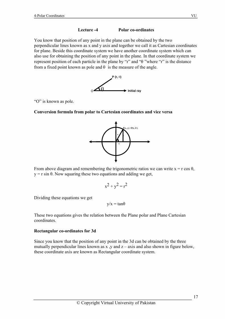
Approaching to (0,0) through x-axis
f (x,y)
Approaching to (0,0) through y-axis
f (x,y)
(0.5,0) 0.25 (0,0.1) -0.1
(0.25,0) 0.0625 (0,0.001) -0.001
(0.1,0) 0.01 (0,0.00001) 0.00001
(-0.25,0) 0.0625 (0,-0.001) 0.001
(-0.1,0) 0.01 (0,-0.00001) 0.00001
Approaching to (0,0) through f (x,y)
y = x
(0.5,0.5) -0.25
(0.1,0.1) -0.09
(0.01,0.01) -0.0099
(-0.5,-0.5) 0.75
(-0.1,-0.1) 0.11
(-0.01,-0.01) 0.0101
© Copyright Virtual University of Pakistan
26

5-Limits of multivariable function VU
Example
f(0,0) is not defined and we see that limit also does not exit.
rough (y = 0)
f (x,y
Approaching to (0,0) through
f (x,y)
Approaching to (0,0) thx-axis
) y = x
( 0.5,0 ) 0 0.5 ( 0.5,0.5 )
( 0.1,0 ) 0 ( 0.25,0.25 ) 0.5
( 0.01,0 ) 0 0.5 ( 0.1,0.1 )
( 0.001,0 ) 0 ( 0.05,0. 0.5 05 )
( 0.0001,0 ) 0 ( 0.001,0.001 ) 0.5
( -0.5,0 ) 0 ( -0.5,-0 0.5 .5 )
( -0.1,0 ) 0 ( -0.25,-0 0.5 .25 )
( -0.01,0 ) 0 ( -0.1,-0.1 ) 0.5
( -0.001,0 ) 0 ( -0.05,-0.05 ) 0.5
( -0.0001,0 ) 0 ( -0.001,-0.001 ) 0.5
li(x,y) → (0,0)
m xy
x2 + y2 = 0 (along y = 0)
lim
(x,y ) → (0,0)
xyx2 + y2 = 0.5 (along y = x)
lim
(x,y ) → (0,0)
xyx2 + y2 does not exist.
f (x,y) = x
xy2+y2
Example lim
( x , y ) → (0, 0 ) xy x 2 + y 2
Let ( x , y ) approach (0, 0) along the line y = x.
f (x , y ) = xy
x 2 + y 2 = x . x
x 2 + x 2 = 1
1 + 1 x ≠ 0.
= 1 2
© Copyright Virtual University of Pakistan
27

5-Limits of multivariable function VU
Let (x , y ) approach (0, 0) along
e line y = 0. th
We can approach a point pace through hs some of t e shown in the figure below Rule for Non-Existence of a Limit
in s infinite pat hem ar.
in
we approach (a, b) along different paths
If We get two or more different values as , then
he paths along which (a, b) is approached may be straight lines or plane curves through
does not exist. T(a, b). Example
Lim(x, y) → (a, b) f(x, y)
f (x , y ) = x. ( 0 )
x + (02 )2 = 0 , x ≠ 0 .
Thus f(x, y) assumalues as (x,y) a
es two different v pproach ) along two different paths.
(
es (0,0
lim x, y) → (0 , 0 )
f (x, y ) does not exist.
x
(x0,y0)
(xy)
Lim ( x , y ) → ( a , b ) f ( x , y)
Lim (x , y ) → (2 , 1 )
x 3 + x 2 y − x − y 2
x + 2 y
= Lim
( x , y ) → (2 , 1 ) (x 3 + 2 x 2 y − xy − 2 y 2 )
Lim ( x , y ) → (2 , 1 )
(x + 2 y )
y
© Copyright Virtual University of Pakistan
28

5-Limits of multivariable function VU
Example
ES FO
ULR R LIMIT
If
0 0 0 01 2( , ) ( , ) ( , ) ( , )
lim ( , ) lim ( , )x y x y x y x y
f x y L and g x y L→ →
= =
a) (if c is constant)
(b)
Then
(
0 01( , ) ( , )
lim ( , )x y x y
cf x y cL→
=
0 01 2( , ) ( , )x y x y
lim { ( , ) ( , )}f x y + =
g x y L L+→
0 01 2( , ) ( , )
lim { ( , ) ( , )}x y x y
f x y g x y L L→
− = −
d) ( 0 0
1 2( , ) ( , )lim { ( , ) ( , )}
x y x yf x y g x y L L
→=
(e) 0 0( , ) ( , )
2( , )x y x y
1( , )lim Lf x y= (if L2 = 0)
g x y L→
0 0( , ) ( , )
limx y x y
c c→
= (c a constant), 0 0
0 0( , ) ( , )lim
x y x yx x
→= ,
0 00 0( , ) ( , )
limx y x y
y y→
=
value of θ.
We set x = r cos θ , y = r sin θ
r cos θ sin , for r > 0
= Lim
( x , y) → ( 2 , 1 ) (x3 + 2 x2 y − x − y2 )
Lim ( x , y) → (2 , 1 )
(x + 2 y )
Lim ( x , y ) → ( 0,0,0 ) xy
x 2 + y
2
th
Similarly for the function of three variables.
since | cos θ sin θ | ≤ 1 for all
= θ
en x
x + 2 y 2 =
r cos θ . r sin θ
r 2 cos2 θ + r
2 sin2 θ
Since r = x 2 + y
2 , r → 0 as ( x , y ) → (0, 0),
Lim ( x , y ) → ( 0 , 0)
xx
2 + y 2 = Lim r → 0r cos θ sin θ = 0,
© Copyright Virtual University of Pakistan
29

5-Limits of multivariable function VU
Overview of lecture# 5 In this lecture we recall you all the limit concept which are prerequisite for this course nd you can find all these concepts in the chapter # 16 (topic # 16.2)of your Calculus By oward Anton.
aH
© Copyright Virtual University of Pakistan
30

6-Geometry of continuous functions VU
Lecture No -6 Geometry of continuous functions
eometry of conGco
tinuous functions in one variable or Informal definition of ntinuity of function of one variable.
function is continuous if we draw its graph by a pen then the pen is not raised so that ere is no gap in the graph of the function
eometry of continuous functions in two variables or Informal definition of ntinuity of function of two variables.
he graph of a continuous function of two variables to be constructed from a thin sheet of ay that has been hollowed and pinched into peaks and valleys without creating tears or inholes.
ontinuity of functions of two variables A function f of two variables is called continuous at the point (x0,y0) if
1. f (x0,y0) if defined.
2.
Ath Gco
Tclp C
0 0( , ) ( , )lim ( , )
x y x yf x y
→ exists.
3.0 0( , ) ( , )
lim ( , )x y x y
f x y→
= f (x0,y0).
he requirement that f (x0,y0) must be defined at the point (x0,y0) eliminates the ossibility of a hole in the surface z = f (x0,y0) above the point (x0,y0).
ustification of three points involving in the definition of continuity. ) Consider the function of two variables
Tp J(1 2 2 2 2ln( )x y x y+ + now as we know that the
og function is not defined at 0, it means that when x = 0 and y = 0 our function L2 2 2 2ln( )x y x y+ + is not defined. Consequently the surface will ave a hole just above the point (0,0)as shown in the graph of
2 2 2 2ln( )z x y x y= + +2 2 2 2ln( )x y x y+ + h
The requir (2) ement that
0 0( , ) ( , )lim ( , )
x y x yf x y
→exists ensures us that the surface z = f(x,y) of
e function f(x,y) doesn’t become infinite at (x0,y0) or doesn’t oscillate widely. th
© Copyright Virtual University of Pakistan
31

6-Geometry of continuous functions VU
Consider the function of two variables2 2
1x y+
l domain
0
hus the limit of the function
now as we know that the Natura
of the function is whole the plane except origin. Because at origin we have x = 0 and y =in the defining formula of the function we will have at that point 1/0 which is infinity.
T 12 2x y+
does not exists at origin. Consequently the
surface 12 2
zx y+
= will approaches towards infinity when we approaches towards
origin as shown in the figure above.
(3) The requirement that
0 0( , ) ( , )lim ( , )
x y x yf x y
→) = f (x0,y0
ensures us that the surface z = n’t have a vertical jump or step above the point (x0,y Consider the functi
0
now as we know that the Natural domain of the function is whole the plane. But you should note that the function has one value “0” for all the points in the plane for which both x and y have nonnegative values. And value “1” for all other points in the plane.
onsequently the surface
z f x y= = ⎨ has a jump as shown in the figure
f(x,y) of the function f(x,y) does0).
on of two variables
0 0( , )
1if x and y
f x yotherwise
≥ ≥⎧= ⎨
⎩
C
0 0 0if x and y≥ ≥⎧( , )
1 otherwise⎩
© Copyright Virtual University of Pakistan
32

6-Geometry of continuous functions VU
Example Check whether the limit exists or not for the function Solution:
First we will calculate the Limit of the function along x-axis and we get 2
2( , ) (0,0)lim ( , ) 1
0x y
xf x yx→
= =+
(Along x-axis)
N it of the function along y-axis and we note that the limit ow we will find out the lim
is2
2( , ) (0,0) 0x y y→lim ( , ) 1yf x y = = (Along y-axis). Now we will find out the limit of the
nd we note tha
+
function along the line y = x a t2
2 2( , ) (0,0)
1lim ( , )2x y
xf x yx x→
= =+
(Along y = x)
0) doesn’t exists because it has different values long different paths. Thus the function cannot be continuous at (0,0). And also note that
the function id not defined at (0,0) and hence it doesn’t satisfy two conditions of the continuity.
xample
olution: First we will note that the function is defined on the point where we have
to check the Continuity that is the function has value at (0,0). Next we will find out the
Limit of the function at (0,0) and in evaluating this limit we use the result
It means that limit of the function at (0,a
ECheck the continuity of the function at (0,0)
S
and note that
⎪⎩⎨
=+=
)0,0(),(1) 22
yxifyx
2
2 2( , ) (0,0)lim ( , )
x y
xf x yx y→
=+
⎪⎧
≠+ )0,0(),()sin(
,(22
yxifyxyxf
0
sinlim 1x
xx→
=
© Copyright Virtual University of Pakistan
33

6-Geometry of continuous functions VU
CONTINUITY OF FUNCTION OF THREE VARIABLES A function f of three variables is called continuous at a point (x0,y0,z0) if
1. f (x0,y0,z0) if defined. 2.
, ) ( , , )lim ( , , )
y z x y z
0 0 0( ,xf x y z
→ exists;
30 0 0( , , ) ( , , )
lim ( , , )x y z x y z
f x y z→
= f(x0,y0,z0).
EXAMPLE
Check the continuity of the function
2 2( , , )1
f x y zx y
1y +=
+ −
ined on the cylinder Solution: First of all note that the given function is not def
R CONTINOUS FUNCTIONS
two then their composition f(x, y) = g(h(x,y)) is a continuous function of x and y.
composition of continuous functions is continuous. ference, or product of continuous functions is continuous.
us, expect where the denominator is zero.
EXAMPLE OF PRODUCT OF FUNCTIONS TO BE CONTINUED
CONTINUOUS EVE
A function f ensional space or 3-dime A function that is continuous at every point in 2-dimensional space or 3-dimensional space is called continuous
In general, any function of the for
2 2 1x y+ − = 0 .Thus the function is not continuous on the cylinder 2 2 1x y+ − = 0 And continuous at all other points of its domain.
RULES FO (a) If g and h are continuous functions of one variable, then f(x, y) = g(x)h(y) is a continuous function of x and y (b) If g is a continuous function of one variable and h is a continuous function ofvariables,
AA sum, difA quotient of continuous function is continuo
mf(x, y) = Axmyn (m and n non negative integers)
is continuous because it is the product of the tinuous functions Axm and yn.
Th unctio
lim
(x,y ) → (0,0)
f(x,y) = lim(x,y ) → (0,0)
Sin(x2 + y2)
x2 + y2
=1 = f(0, 0)
This shows that f is continuous at (0,0)
con
e f n f(x, y) = 3x2y5 is continuous because it is the product of the continuous
functions g(x) = 3x2 and h(y) = y5.
RYWHERE
that is continuous at each point of a region R in 2-dimnsional space is said to be continuous on R.
everywhere or simply continuous.
© Copyright Virtual University of Pakistan
34
6-Geometry of continuous functions VU
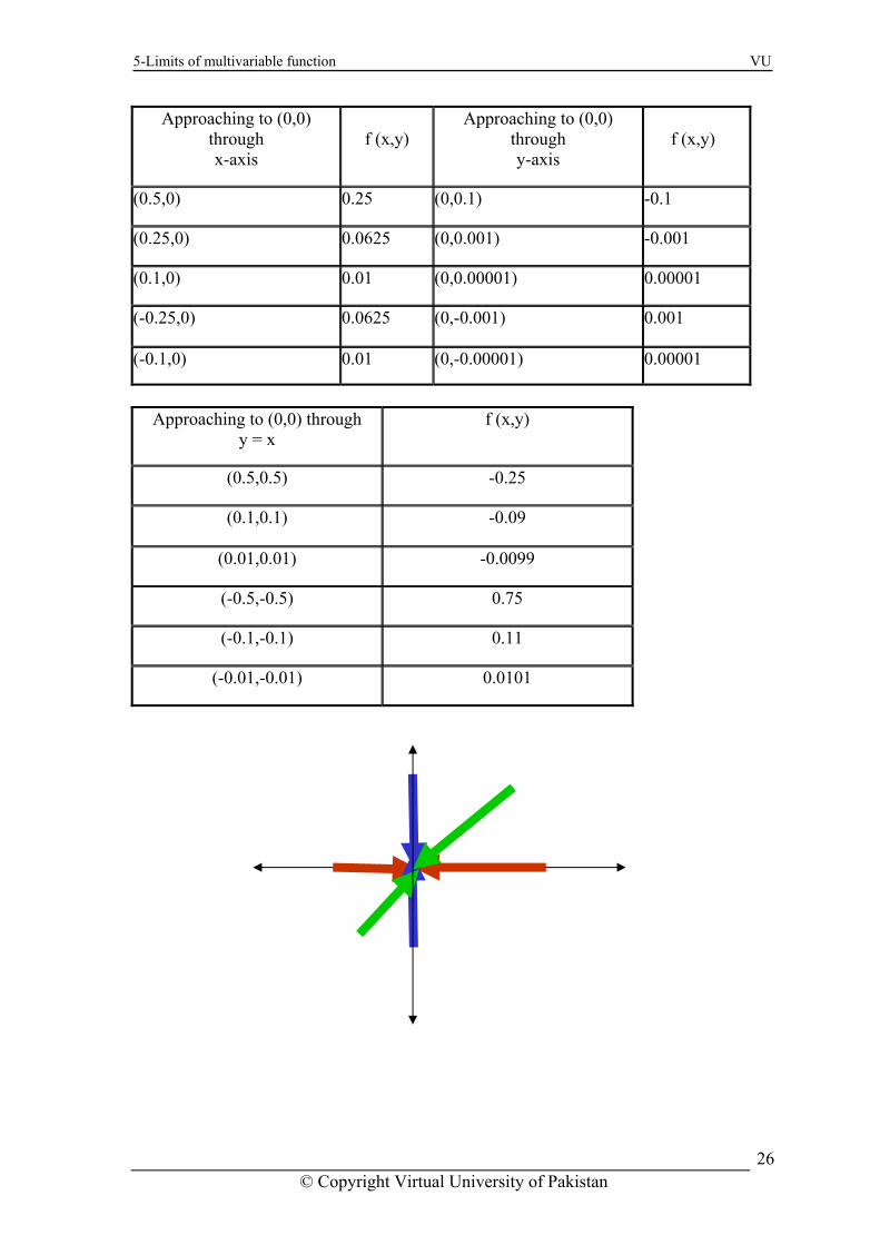
Example: (
1)f
The function f is continuous inis shown in figure below.
(x,y) = ln(2x – y +1) the whole region where 2x > y-1, y < 2x+1.And its region
y < 2x+1
(2)1( , ) xyf x y e −=
The function f is continuous in the whole region of xy-plane. (3) 1, ) tan ( )(f x
he whole region of xy- plane. y y x−= −
The function f is continuous in t( , )f x y y x= − (4)
The function is continuous where x ≥ y
yx ≥ y
Let
the
x = x o 0artial
erivative of f with respect of x at the point (xo , y0) .
x constant, say x = x0 and view y as a variable, then f (x0 , y ) is a
function is differentiable at y = y , then the value of this
0 0of y at the point (x0 , y0)
Partial derivative
f be a function of x and y. If we hold y constant, say y = y0 and view x as a variable,
n f(x, y0) is a function of x-alone. If this function is differentiable at
xo, then the value of this derivative is denoted by f (x , y ) and is called the P
d
Similarly, if we hold
function of y alone. If this 0derivative is denoted by fy (x , y ) and is called the Partial derivative of f with respect
© Copyright Virtual University of Pakistan
35

6-Geometry of continuous functions VU
Example 2 ( , ) 2 43 2f x y x y y x= + +
ubstituting x = 1 and y = 2 in these partial-derivative formulas yields.
fx (1, 2) = 6(1)2(2)2 + 4 = 28 fy (1, 2) = 4(1)3(2) + 2 = 10
t
x
ting x as a constant a differentiating
fy (x, y) = 4x3y + 2
g y as a constant and differentiating Trea inwith respect to x, we obtain
(x, y) = 6x2y2 + 4 fTrea ndwith respect to y, we obtain
S
Example
Z = 4x2 - 2y + 7x4y5
Example
2 2( , )z f x y x sin y= = Then to find the derivative of f with respect to x we treat y as a constant therefore
44352
288
yxz
yxxx
+−=∂
+=∂
53z∂
y∂
22z sinxf x yx∂
d the derivative of f with respect to y we treat x as a constant therefore
∂= =
Then to fin2
2
2sin cos
sin 2
yz f x yy
x y
∂= =
∂
=
y
Example
2 2
ln x yzx y
⎛ ⎞+= ⎜ ⎟+⎝ ⎠
By using the properties of the ln we can write it as z = ln(x2 + y2) − ln (x + y) ∂z
∂y
Similarly, (or by symmetry) ∂z
= y2 + 2xy − x2
2 2)(x + y)(x + y
∂x = x2 + y21
. 2x − x + y1
= 2x2 + 2xy − x2 − y2
(x2 + y2)(x + y)
= x2 + 2xy − y2
(x2 + y2)(x + y)
© Copyright Virtual University of Pakistan
36

6-Geometry of continuous functions VU
Example
xample
xample
∂w∂x = 2x – yz
∂wdy = 6y - xz
dwdz = 8z - xy
w = x2 +3y2+4z2-xyz
z = cos(x5y4)
)()sin( 4545 yxx
yxxz
∂∂
−=∂∂
)sin(5 4544 yxyx−=
)()sin( 4545 yxy
yxyz
∂∂
−=∂∂
)sin(4 4535 yxyx−=
4 3
4 3 3 4
4 3 3 3
sin( )
sin( ) sin( ) ( )
cos( ) sin( )4
z x xy
4 3sin( )z x xyx x
E
E
3
4 3 3 3cos( ) sin( )
x xy xy xx x
x xy y xy x
x
=∂ ∂ ⎡ ⎤= ⎣ ⎦
z x y xy xy∂= +
∂ ∂∂ ∂⎡ ⎤= +⎣ ⎦∂ ∂
= +
∂
4 3
4 3 3 4
4 3 2 3
5 2 3
sin( )
sin( ) sin( ) ( )
cos( ).3 sin( ).03 cos( )
z x xyy y
x xy xy xy y
x xy xy xyx y xy
∂ ∂ ⎡ ⎤= ⎣ ⎦∂ ∂∂ ∂⎡ ⎤= +⎣ ⎦∂ ∂
= +
=
© Copyright Virtual University of Pakistan
37
7-Geometric meaning of partial derivative VU
Lecture No -7 Geometric meaning of partial derivative Geometric meaning of partial derivative
z = f(x, y) Partial derivative of f with respect of x is denoted by
artial derivative of f with respect of y is denoted by
Partial Deri
P
vatives Let z = f(x, y) be a function of two variable defined on a certain dom
∆x in x, keeping y as it is, th
∆z = f (x + ∆x, y) – f (x, y)
ain D. For a given change e change ∆z in z, is given by If the ratio
proaches to a finite limit as ∆x →0, then this limit is called Partial derivative of f with spect of x.
Sim ∆z in z, is given by
the ratio
pproaches to a finite limit as ∆y →0, then this limit is called Partial derivative of f with spect of y.
∆y
apre
ilarly for a given change ∆y in y, keeping x as it is, the change ∆z = f (x , y + ∆y) – f (x, y)
If
∆z
= f(x , y+ ∆y) − f(x, y)
are
∆y
∆ z∆ x = f(x + ∆ x, y)−f(x, y)
∆ x
∂ z
∂ x or fx or
∂ f ∂ x
∂ z
∂ y o r fy or
∂ f
∂ y ,
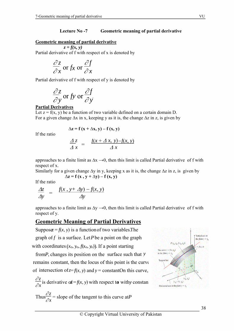
eometric Meaning of Partial DerivativesGSuppose z = f ( x , y ) is a function of two variables.Thegraph of f is a surface. Let P be a point on the graph
( xo, y o , f ( x o , yo ) ) . If a point starting from P , changes its position on the surface such that
constant, then the locus of this point is the curvez= f (x, y ) and y = constant.On this curve,
∂ z ∂ x
is derivative of z = f ( x , y ) with respect tox with y constant
Thus ∂ z ∂ x
= slope of the tangent to this curve at P
y
intersection of
with coordinates
roemains
f
© Copyright Virtual University of Pa
.
kistan
38

7-Geometric meaning of partial derivative VU
he figure below (left) Also together these tangent lines are shown in figure
As shown in tbelow (right).
Similarly, tangent at to the curve of
intersection of z = f (x , y ) and x = constant.
Partial Derivatives of Higher Orders
P
∂ z ∂ y is the gradient of the
The partial derivatives f x and fy of a function f of two variables x and y , being functions of x and y, may possess derivati ves. In such cases, the
second order partial derivatives are defined as below.
∂ ∂ x ⎝
⎜ ⎛ ⎠ ⎟ ⎞
∂ f∂ x
= ∂2f
∂ x2 = ∂
∂ x (fx) = (fx)x = fxx = fx2
∂
Example
⎝ ⎜ ⎛
⎠ ⎟ ⎞
∂ f∂ y =
∂ 2f∂ y 2 =
∂∂ y (fy) = (fy)y = fyy = fy 2
Thus, there are four second order partial derivatives for a function z = f( x , y ). The partial derivatives fxy and fyx are called mixed second partials and are not equalorder more than two can be defined in a sim
in general. Partial derivatives of ilar manner.
z = arc sin ⎝ ⎜ ⎜ ⎛
⎠ ⎟ ⎟ ⎞
xy . ∂ z
∂ x =
1
1 − x 2
y 2
. 1 y =
1
y2 − x 2
∂ z ∂ y
= 1
1 − x 2
y 2
. − x y 2 =
− x
y y2 − x 2
∂ 2 z ∂ y ∂ x
= ∂
∂ y ⎝ ⎜ ⎛
⎠
⎞ ∂ z ∂ x
= − 12 (y2 − x 2)− 3/2.2y
=− y
(y2 − x 2)3/2
∂ y ⎝ ⎜ ⎛
⎠ ⎞
∂ f∂ x
= ∂ 2f∂ y∂ x =
∂∂ y (fx) = (fx)y = fxy
∂
∂ x ⎝ ⎜ ⎛
⎠ ⎞
∂ f∂ y
= ∂ 2f∂ x∂ y =
∂∂ x (fy) = (fy)x = fyx
∂
∂ y
© Copyright Virtual University of Pakistan
39

7-Geometric meaning of partial derivative VU
∂ 2 z Example Laplace’s Equation For a function w = f(x,y,z)
∂ x ∂ y = ∂
∂ x ⎝ ⎜ ⎛
⎠ ⎟ ⎞
∂ z ∂ y
= − 1
y y2 − x2 − xy
⎣⎢⎡
⎦⎥⎤x
(y2 − x2)3/2
= − y2 + x2 − x 2
y(y 2 − x2 )3/2 = − y(y2 − x2)3/2
Hence
∂ 2 z ∂ x ∂ y
= ∂ 2 z
∂ y ∂ x
xyeyxy x f += cos),(xye y
x
f + =
∂
∂ cos
xeyx
f y x y
f +−=
⎠ ⎞
⎜ ⎝ ⎛
∂
∂
∂
∂ =
∂ ∂ ∂ sin
2
xyex
f x x
f =
⎠ ⎞
⎜ ⎝ ⎛
∂
∂
∂
∂ =
∂
∂ 2
2
f(x, y) = x cosy + y e x
∂ f
∂ y
= − x siny + ex
∂ 2 f
∂ x ∂ y
= − siny + ex
∂ 2 f
∂ y 2 =
∂
∂ y
⎝ ⎜ ⎛
⎠
⎞ ∂ f
∂ y
= -x cos y
The equation
∂ 2f
∂ x2 +
∂ 2f∂ y2 ∂ 2f
∂ z2 = 0
is called Laplace’s equation .
© Copyright Virtual University of Pakistan
40

7-Geometric meaning of partial derivative VU
Example
dding
A both partial second order derivative, we have Euler’s theorem The mixed derivative theorem
f(x,y) and its partial derivatives fx, fy, fxy and fyx are defined throughout
n open region containing a point (a, b) and are all continuous at (a, b), then
fxy(a , b) = fyx (a , b)
dvantage of Euler’s theorem
If
a
A
he sym t with respect to y and then with respect x. Howith respect to x, we get the answer more quickly.
T bol ∂2w/ ∂x ∂y tell us to differentiate firsto ever, if we postpone the differentiation with respect to y and differentiate first w Overview of lecture# 7 Chapter # 16 Partial derivatives
age # 790 Article # 16.3
f ( x , y ) = ex sin y + e y cos x ,∂ f ∂ x = e x sin y − e y sin x
∂ 2f
∂ x2 = ex sin y − e y cos x
∂f ∂y = ex cosy + e y cosx
∂2 f
∂y 2 = -e xsiny +ey cosx
2 ∂ f
∂ x2 + ∂ 2 f
∂ y 2 = ex sin y − ey cos x
− e x sin y + eycos x =0
12 ++=
y exy w
y
12
=∂∂
∂xy
wy
xw =
∂∂
P
© Copyright Virtual University of Pakistan
41

8-Euler theorem chain rule VU
Lecture No- 8 More About Euler Theorem Chain Rule
In general, the order of differentiation in an nth order partial derivatice can be change without affecting the final result whenever the function and all its pa For example, if f and its partial order derivatives of the firs ers are continuous
e set,
yyxyxy
rtial derivatives of order ≤ n are continuous.t, second, and third ordf thon an open set, then at each point o
xyy fff ==
ther notation.
or in ano
Order of differentiation
22 yxf
yxyf
xyf
∂∂∂
=∂∂∂
∂=
∂∂∂
For a f
we and th king the job difficult. But if we
with respect to y, firstly and then with respect to x secondly rivative can be calculated in a few steps.
unction
If re interested to find , that is, differentiating in the order firstly w.r.t. x a en w.r.t. y, calculation will involve many steps madifferentiate this functionthen the value of this fifth order de
333
yx
f (x ) = ,y y2x4ex + 2
EXAMPLE
yxy +=)
xf−
,(
2)(
)()()()(),(
yx
yxx
yxyxx
yxyxfx −
−∂∂+−+
∂∂−
=
2)(
)1)(()1)((yx
yxyx−
+−−=
2)(
2yxy
−−
=
∂ 5f ∂y 3 ∂x2
03 2
5 =
∂∂∂
y x
f
2) (
) ( ) ( ) ( ) (
) , ( y x
y x y
y x y x y
y x
y x f y −
− ∂
∂ + − + ∂
∂ −
=
2 ) (
) 1 )( ( ) 1 )( (
y x
y x y x
−
− + − −
=
2 ) (
2
y x
x
− =
© Copyright Virtual University of Pakistan
42

8-Euler theorem chain rule VU
EXAMPLE
xye x y x f y sec), ( 33 +=
−
xye
EXAMPLE
xample
E
)sin(3 xyyxf y
),( x−=
)sin()(),( 23
21
21 ππ −=yf
81−=
)cos(),( 2 xyxyxf =
)sin()cos(2),( 2 xyyxxyxyxfx −=
)2sin()()21()2cos()2
1(2),21( 2 ππππ −=x
f
4π−
xyxyy yexexyx 32),( +=
)1(2 xyex xy +=
)]1)(1(1[)1)(1()1,1( )1)(1( += ey
e2=
xyyexyxf 2),( =
xyxyx eyxxyeyxf 222),( +=
)2( xyxyexy +=
)]1)(1(2[)1)(1()1,1( )1)(1( += ef x
e3=
xyyexyxf 2),( =
=
f
f
xyxf x
xx ye xyx
yy
yx
sec3 ) , (
2tansec3 ) , (
23
3 2
+ − =
+ =
−
1− f
© Copyright Virtual University of Pakistan
43

8-Euler theorem chain rule VU
EXAMPLE
hain
C Rule in function of One variable Given that w= f(x) and x = g(t), we find as follows:
f(x), we get
xample
From w = From x = g(t), we get Then E
5)234 ( zyx w +− =
4) 2 3 4 ( 20 z y x x
w + − = ∂
∂
32
) 3 4 ( 24 2z y x x y
w + − − = ∂ ∂
∂
3
x y z
w =−1440(4x−3y+2z)2
∂ ∂ ∂
∂
) 2 3 4 ( 5762
4
z y x x y z
w + − − = ∂ ∂ ∂
∂
dwdt
dwdx
dxdt
dw
dt =
dw
dx
d xdt
w = x + 4 , x = Sint By Substitution w = Sint + 4 dw
dt
= Cost
w = x + 4 ⇒ dwdx
= 1
x = Sint ⇒ dxdt
= Cost
By Chain Rule dwdt
= dwdt
× dxdt
= 1 . × Cost = Cost
© Copyright Virtual University of Pakistan
44

8-Euler theorem chain rule VU
), y = f(t)
XAMPLE BY SUBSTITUTION
w = f(x,y), x = g(t
E
Chain rule in functionof one variable
w = xyx = cost, y = sint
y is a function of u, u is a function of vv is a function , w is a function of z
. Ultimately y is function of x
lk about dydx
of wz is a function of x
so we can ta
and by cha le it is given by dydx
in ru
= dydu
dudv
dvdw
dwdz
dzdx
x y
t
wx
∂∂
wy
∂∂
dxdt
dydt
dw w dx w dy∂ ∂dt x dt y dt
= +∂ ∂
Independent variables
Dependent variable w = f(x,y)
Intermediate variables
w = cost sint
= 12 2 sint cot
= 12 sin2t
dwdt =
12 cos2t.2
= cos 2t
© Copyright Virtual University of Pakistan
45

8-Euler theorem chain rule VU
EXAMPLE
EXAMPLE
EXAMPLE
z = 3x2 y3 x = t4 , y = t2
x
∂z∂
= 6xy , ∂y3 ∂z
= 9 x y
dxdt
2 2
= 4t3, dy
dt = 2t
dwdt =
∂w∂x
dxdt +
∂w∂y
dydt
dxdt = − sint,
z = 1 + x ln- 2xy
4 x = y = t
zx
∂∂
= 1
2 1 + x - 2xy 4
∂z∂y
= 1
2 1 + x - 2xy 4 .(- 8xy 3) =
- 4xy 3
1 + x - 2xy 4
dx
dt = 1
t ,
ddt
=
, cos ,and sinw xy x t y t= = =∂ w
∂ y = x ∂ w
∂ x = y
dy
dt = cost,
(sin )( sin ) (cos )(cos )t t t t= − +t t t 2 cos cos - sin
2 = + =
dz
dt =
∂ z
∂ x dx
dt +
∂ z
∂ y dy
dt
= (6xy 3 ) (4t 3 ) + 9x 2 y 2 (2t) = 6 (t 4 ) (t 6 ) (4t 3) + 9 (t 8 ) (t 4 ) (2t) = 24 t 13 + 18t 13 = 42t 13
2
© Copyright Virtual University of Pakistan
46

8-Euler theorem chain rule VU
XAMPLE E
verview of Lecture#8
w = f(x,y,z), x = g(t) ,y = f(t), z = h(t)
O
opic # 16.4 age # 799 Book Calculus By Haward Anton
Chapter # 16 T P
w = f(x,y,z)
y z
t
wx
∂∂ w
y∂∂
wz
∂∂
dxdt
dydt
dzdt
Independent variables
Dependent variable
dzdt
=
∂ z ∂ x
dx dt
+ ∂ z ∂ y
. dy dt
1 – 2y4 =
2 1 + x - 2xy4 t 1
t -
4xy 3
1 + x - 2xy4 . 1
= 1
1 + x - 2xy 4 ⎣ ⎢ ⎡
⎦ ⎥ ⎤ 1–
4
2t - 4xy3
= 1
1 + lint - 2 (lnt ) t 4
⎣ ⎢ ⎡
⎦ ⎥ ⎤ 1-2t4
2t - 4 (lnt) t3
= 1
1 + lnt - 2t 4 lnt
⎣ ⎢ ⎡
⎦ ⎥ ⎤ 1
2t - t3 - 4t 3 lnt
z = ln (2x 2 + y) x = t , y = t
2/3
∂z∂x
= 1
2x 2 + y . 4x =
42x 2 + y
∂z∂y
= 2x1 2 + y
, dx dt
= 12 1
t ,
dy dt =
23 t
-1/3
© Copyright Virtual University of Pakistan
47

8-Euler theorem chain rule VU
Lecture No - 9 Examples
First of all we revise the example which we did in our 8th lecture.
onsider w = f(x,y,z) Where x = g(t), y = f(t), z = h(t)
w = f(x), where x = g(r, s). Now it is clear from the figure that “x” is intermediate variable and we can write.
C Then
Example:
Consider
dtdz
zw
dtdy
yw
dtdx
xwdw
dt ∂∂+
∂∂+
∂∂
w = x2 + y + z + 4 tx = e , y = cost, z = t + 4
∂w∂x = 2x,
∂w∂y = 1,
∂w∂z = 1
dxdt = et ,
dydt = −Sint,
dzdt = 1
dwdt =
∂w∂x
dxdt +
∂w∂y
dydt +
∂w∂z .
dzdt
= (2x) (et) + (1) . (− Sint) + (1) (1) = 2 (et) (et) − Sint + 1 = 2 e2t − Sint + 1
and Example: w = Sin x + x2, x = 3r + 4s dwdx = Cosx + 2x
∂x∂r = 3
∂x∂s = 4
w∂∂r =
dwdx .
∂x∂r
os (3r
∂s
= (Cosx + 2x) . 3 = 3 Cos (3r+4s) + 6 (3r + 4s) = 3 C + 4s) + 18r + 24s ∂w
=
Dependent variable
w = f(x)
Intermediate variables
dwdx
x
xr
∂∂
xs
∂∂
s
w dw xr dx r
∂ ∂=
∂ ∂w ds
∂ ∂∂
w xdx s
=∂
= w
dxd
. ∂x∂s
= (Cosx + 2x) . 4 = 4 Cosx + 8x
(3r + 4s) + 8 (3r + 4s) = 4 Cos (3r + 4s) + 24r + 32s
= 4 Cos
© Copyright Virtual University of Pakistan
48

9-Examples VU
Consider the function w = f(x,y), Where x = g(r, s), y = h(r, s)
wy
∂∂
Similarly if you differentiate the function “w” with respect to “s” we will get
∂ w∂ r =
∂ w∂ x
∂ x∂ r +
∂ w∂ y
∂ y∂ r
Dependent variable w = f(x,y)
wx
∂∂
x Intermediate variables y
r s r r
xr
∂∂ x
s∂∂ y
r∂∂
ys
∂∂
And we have
w ∂∂s =
∂x∂w
∂s∂x
+ ∂w∂y
∂s∂y
© Copyright Virtual University of Pakistan
49

9-Examples VU
© Copyright Virtual University of Pakistan 50
Consider the function w = f(x,y,z), Where x = g(r, s), y = h(r,s), z = k(r, s)
Thus we have
Similarly if we differentiate with respect to “s” then we have,
Consider the function
ow as we know that By putting the values from above
ow
∂w∂s
= ∂w∂x
∂x∂s +
∂w∂y
∂y∂s +
∂w∂z
∂z∂s
∂w∂r =
∂w∂x
∂x∂r +
∂w∂y
∂y∂r +
∂w∂z
∂z∂r
Depende t variabn le w = f(x,y,z)
x z intermediate variables y
r
Example: First we will calculate Nwe get N So we can calculate
xr∂
∂xs∂
∂
s
y∂r∂
r p
ys
∂∂
r s
zr
∂∂
zs
∂∂
Independent variables
22 ,w x y z= + + ,rxs
= 2 ln ,y r s= + 2z r=
1wx
∂=
∂ 2w
y∂
=∂
2w zz
∂=
∂1 x
r s∂
=∂
2y rr
∂=
∂ 2z
r∂
=∂
w w x w y w z∂ ∂ ∂ ∂ ∂ ∂ ∂= + +
r x r y r z r∂ ∂ ∂ ∂ ∂ ∂ ∂
1(1) (2)(2 ) (2 )(2)w r zr s
δδ
⎛ ⎞= + +⎜ ⎟⎝ ⎠
1 4 (4 )(2)r rs
= + +1 12rs
= +
2 x rs s
∂= −
∂1 y∂
=∂s s
0zs
∂=
∂
s x y r z r
= + +∂ ∂ ∂ ∂ ∂ ∂ ∂
w w y w zr
∂ ∂ ∂ ∂x∂ ∂ ∂ w
2
rs s⎝ ⎠ ⎝ ⎠
1(1) (2) (2 )(0)z⎛ ⎞ ⎛ ⎞= − + +⎜ ⎟ ⎜ ⎟
2
2 rs s
= −

9-Examples VU
© Copyright Virtual University of Pakistan 51
Remembering the different Forms of the chain rule: The best thing to to d by placing the dependent variable
n top, the intermediate variables in the middle, and the selected independent variable at the bottom. To find the derivative of dependent variable with respect to the selected independent variable, start at the dependent variable and read down each branch of the
pendent variable, calculating and multiplying the derivatives along the branch. Then add the products you found for the different branches.
and
⎝⎜⎛
⎠⎟⎞
do is raw appropriate tree diagramo
tree to the inde
Example:
Taking “ln” of both sides of the given equation we get Now Taking partial derivative with respect to “r, s , u , and t” we get , ,
∂ω∂x ,
∂ω∂y ……
∂ω∂υ
and ⎝⎜⎛
⎠⎟⎞∂x
∂p , ∂y∂p ……
∂υ∂p
Derivatives of ω withrespect to the
ariable
Derivatives of the intermedaitevariables with respect to the
endent variable
The other equations are obtained by replacing p by q, …, t, one at a time. One way to remember last equation
k of the right-hand side as oduct of two vectors with
components.
ω
∂p
intermedaite v s selected indep
is to thinthe dot pr
∂ =
∂ω ∂x∂x ∂p +
∂ω ∂y∂y ∂p + …… +
∂ω ∂υ∂υ ∂p .
S uppose ω = f ( x, y, … ., υ ) is a d iffe re nt iab le func t io n o f the
iab les x, y, … .., υ (a fin ite υ are
q , , t set ). T he n ω is a
d iffe re nt iab le func t io n o f the var iab les p thro ugh t a nd the part ia l der ivat ives o f ω w ith
the se var iab le s are t io ns o f the form
The Chain Rule for Functions
r re w e w e= ⇒ =
of Many Variables
varset) a nd the x, y, … , d iffe re nt iab le funct io ns o f p ,(ano ther fin ite
respect to g ive n b y eq ua
ln( )r s t uw e e e e= + + +
w r s t ue e e e e= + + +
r w− w s s ws se w e w e −= ⇒ =
w u u wu ue w e w e −= ⇒ =
t te w ww t t we e −= ⇒ =
w r

9-Examples VU
Now since we have Now Differentiate it partially w.r.t. “s” (Here we use the value of sw ) Now differentiate it partially w.r.t. “t” and using the value of we get,
Now differentiate it partially w.r.t. “u” we get,
, we get,
r s t u wrstu
e
w e
+ + − −
+ + + −= −
r wrw e −=
( )r wrs sw e w−= −
r w s we e− −= −2r s w
rsw e + −= −
2 ( 2 )r s wrst tw e w+ −= − −
32 r s t wrstw e + + −=
22 r s w t we e+ − −=
tw
32 ( 3 )r s wrstu uw e w+ −= −
uwand by putting the value of
36 (4
)
6
r s t w u wrstuw e= −
© Copyright Virtual University of Pakistan
52

11-The triple scalar or Box product VU
Lecture No -10 Introduction to vectorsagnitude. But some times
the es. n hat force is acting
w large it is (Magnitude). ther Example is the body’s Velocity; we have to know where the body is headed as well how fast it is. uantities that have direction as well as magnitude are usually represented by arrows that int the direction of the action and whose lengths give magnitude of the action in term a suitably chosen unit. vector in the plane is a directed line segment.
B
Some of things we measure are determined by their mwe need magnitude as well as direction to describe quantitiFor Example, To describe a force, We need directio in which t(Direction) as well as hoOasQpoofA
v A
v AB= Vectors are usually described by the single bold face roman letters or letter with an arrow.
he vector defined by the directed line segment from point A to point B is written as AB
agnitude or Length Of a Vector :
T. M
agnitude of the vector is denoted by vM v = AB is the length of the line segment AB
nit vector U
nit vector in the direction
Any Vector whose Magnitude or length is 1 is a unit vector.
of vector v is denoted by v . Uand is given by
vv = v
Addition Of Vectors
O
b
r
This diagram shows three vecto ctors ors, in two vevector AB . The tail of third vector OB is connecte
nne ith the head of vector co cted w AB .This third v
© Copyright Virtual Univer
B
a
e vector OAn d with the tail ector is called
sity of Pakistan
A
is connected with tail of of OA and head is Resultant vector.
53

11-The triple scalar or Box product VU
The resultant vector can be written as r = a + b
Similarly
Equal vectors magnitude and dire
Opposite vectors
opposite direction.
Two vector are para
where
f E
F
r O
r = a + b + c + d + e + f
Two vectors are equal or same vectors if they have same ction.
Two v
llel if on
λ is a non
a b
c
d e
A
C
D
B
b
© Co
a
ectors are
Pe vector i
zero scaaλ=
pyright V
a
opposite vectors if they have same magnitude and
a
-a
arallel vectors s scalar multiple of the other.lar.
irtual University of Pakistan
54

11-The triple scalar or Box product VU
r = x i+ y j + z k
Addition and subtraction of two vectors in rectangular component:
th component of first vector is added (subtracted) to the ith component of second vector, first vector is added (subtracted) to the jth component of second vector,
milarly kth compone nt of
ultiplication of a vector by a scalar
I jth component ofsi nt of first vector is added (subtracted) to the kth componesecond vector, M
ny vector a
Let a = a1i + a2j + a3kand b = b1i + b2j + b3k a + b = (a1i + a2j + a3k) + (b1i + b2j + b3k) = (a1 + b1 )i + (a2 + b2 )j + (a3 + b3)k a - b = (a1i + a2j + a3k) - (b1i + b2j + b3k) = (a1 - b1 )i + (a2 - b2 )j + (a3 - b3)k
a 2a 3a -2a A can be written as
Scalar product
aaa ˆ=
roduct) (“a dot b”) of vector a and b is the
number a.b = |a| |b| cos θ.
where θ is the angle between a and b. In word, a.b is the length of a times the length of b times the cosine of the angle between a and b.
Scalar product (dot p
© Copyright Virtual University of Pakistan
55

11-The triple scalar or Box product VU
Remark:- a.b = b.a
This is known as commutative law. Some Results of Scalar Product
a.b = |a| |b| cos θ. 1. a b If
This means that if a is perpendicular to b. Then a.b=0 Also i.j= 0 = j.i
k.i= 0 =i.k
2. If a b That means a is parallel to b. Then a.b a b
if we replace b by a then
so i.i=j.j=
xample
j.k= 0 =k.j
a.a = a a
a.a = a a a.a
k.k=1
E
If a = 3
k and b = 2 i
+ 2 k
,
then
a . = | a | | b | cos θ
= (3) (2) cos π
4
= 6 . 2
2
= 3 2 .
⊥
||
= | | | |
| | | |
| | 2
| = |
© Copyright Virtual University of Pakistan
56

11-The triple scalar or Box product VU
EXPRE SSION FOR a.b IN COMPONENT FORM
In dot product ith component of vector a will multiply with ith component of vector b , jth com ultiply with jth component of vector b and kth com ultiply with kth component of vector
Example
ponent of vector a will mponent of vector a will m
b
a and b are perpendicular if and only if a.b = 0. This has two parts If “a” and “b” are per perpendicular then a.b=0. And if a.b=0 “a” and “b” will be perpendicular.
Perpendicular (Orthogonal) Vectors
A n g le c t o rs
a = i − 2j − 2k and b = 6i + 3j + 2 k. a.b = (1)(6) + ( − 2)(3) + ( − 2) (2) = 6 − 6 − 4 = − 4| a | =
B e t w e e n t w o v e
(1 )2 + ( − 2 )2 + (− 2)2 = 9 = 3
| b | = ( 6 ) 2 + ( 3 )2 + ( 2 )
2 = 49 = 7
θ = cos - 1
⎝⎜⎛
⎠
⎞
| a.b
| a || b
= cos - 1
⎝⎜⎛
⎠
⎞ − 4
(3 ) (7 ) = cos-1
⎝⎜⎛
⎠⎞
− 4
21 ≈ 1.76 rad
a = a i + a 2 1 j + a 3 k and b b k a .b = ( b 3 k ) = a 1 i + b 2 j + b 3 k ) + a 2 j . (b 1 i + b 2 j + b 3 k ) 2 j + k j + + a b j . i + a 2 b 2 j . j + a 3 b 3 k . k 1 ) a 3 0 ) + a 2 b1 (0 ) + a 2 b 2 (1 ) 2 b 3 1 (0 ) + + a 3 b 2 (0 ) + a 3 b3 (1 ) 3
The angle between two nonzero
vectors a and b is
θ = cos - 1
= b 1 i + b 2 j + 3a 1 i + a 2 j + a 3 k ) . (b 1 i + b 2 j + 1 i . (b
+ a 3 k . (b 1 i + b b 3 ) i. a b i . k = a 1 b 1 i . i + a 1 b 2 1 3 2
+ a 2 b 3 j . k + a 3 b 1 k . i + + a 3 b2 k . j= a 1 b 1 ( + a 1 b2 (0 ) + 1 b (
+ a b+ a 3 (0 ) = a 1 b 1 + a b + a2 2 b3
⎝ ⎜ ⎛
⎠
⎞ a. b
| a || b |
Since the values of the arc i
lie in [0, π ], above equation automatically
gives the angle made by a and b .
© Copyright Virtual University of Pakistan
57

11-The triple scalar or Box product VU
Vector Projectio Consider the Projection of a vector b on a vector a making an angle θ with each other
From right angle triangle OCB e / hypotenuse
COS =
Example
COS =Bas
O C
B
a
b
θ A
|→
OC| = | | Cosθ
= | b| |a | Cos θ
|a|
b
= | a | b.a = b . |a |
a
= ab . |a|
θ
θ
| OC | →
| b |
The number | b | cos θ is called the scalar component of B in the direction of a .
s ince | b | cos θ = B. a
| a | ,
we can find the scalar component by
“ dotting ” b with the direction of a
Vector Projection of b = 6 i + 3 j + 2 k
onto a = i - 2 j − 2 k is
a b = b . a
a . a a
= 6 − 6 − 4
1 + 4 + 4 ( i − 2 j − 2 k )
= − 4
9 ( i − 2 j − 2 k )
= 4
9 i +
8
9 j +
8
9 k .
proj
© Copyright Virtual University of Pakistan
58

11-The triple scalar or Box product VU
ight-hand rule
R
e start with two nonzero nonparallel vectors A and B .We select a unit vector n erpendicular to the plane by the right handed rule. This means we choose n to be the it vector that points the way your right thumb points when your fingers curl through the
ngle 0 from A to B . he vector A*B is orthogonal to both A and B.
lts of Cross Product
WPnu
aT Some Resu
T h e C ro s s P r o d u c t o f T w o V e c to r s in S p a c e
a
T he scalar component
the direction of a of b in
| b |cos θ = b . | a | = (6 i + 3 j + 2 k ).
⎝ ⎜ ⎛
⎠
⎞ 1
3 i − 3
2 j − 3
2 k
4 = 2 − 2 − 3
= − 3
4 .
Consider t wo nonzero vectors a and b in space. T he vec t or product a × b (“ a cross b ” ) to be the vector a × b = (| a | | b | sin θ ) n where n is a vector determined by right hand rule.
© Copyright Virtual University of Pakistan
59

11-The triple scalar or Box product VU
The Area of a Parallelogram
j
k
× b = |a | |b | Sin a θ n a ||b en a × b = 0 a × a = 0
× i = j × j = k × k = 0 a ⊥ b en a × b = |a | |b | n
i × j = k , j × i = − k j × k = i , k × j = − i k × i = j i × k = − j
IfthSoi Ifth N o te tha t th is p roduc t is no t com m uta tive .
i
e ma gnitude of a Because n is a unit
× b is
× b | = | a | | b | |sin
thθ | | n |
| a = |A| | b | sin θ
This is the area of the ll l
termined by a and b
| a | being the base of the de
ll l
and | b | |sin θ | the h i h
© Copyright Virtual University of Pakistan
60

11-The triple scalar or Box product VU
a × b from the components of a and b
Example: Let
a = 2i + j + k and b = − 4i + 3j + k . Then
2 1 14 3 1
i j ka b× =
−
(1 3) (2 4) (6 4)a b i j k× = − − + + + 2 6 10a b i j k× = − − + is the required cross product of a and b.
Over view of Lecture # 10 Chapter# 14 Article # 14.3, 14.4
age # 679
Sua
ppose = a 1 i + a 2 j + a 3k , = b 1 i + b 2 b j + b 3k .
b = (a 1 i + a 2a × j + a 3 k ) × (b 1 i + b 2j + b 3k )
= a 1 b 1 i × i + a 1 b 2 i × j + a 1b 3i × k
+ a 2 b 1 j × i + a 2 b 2 j × j + a 2b 3j × k
+ a 3 b 1k × i + a 3 b 2 k × j + a 3b 3k × k
= (a 2 b 3 − a 3 b 2 ) i − (a 1 b 3 − a 3b 1) j
+ (a 1 b 2 − a 2 b 1 ) k . a = a 1 i + a 2 j + a 3 k ,
b = b 1 i + b 2 j + b 3 k .
a × b =
⎪ ⎪ ⎪ ⎪
⎪ ⎪ ⎪ ⎪
i j k
a 1 a 2
a 3
b 1 b 2
b 3
P
© Copyright Virtual University of Pakistan
61

11-The triple scalar or Box product VU
Lecture No -11 The Triple Scalar or Box Product
he product (a×b) . c is called the triple scalar product of a, b, and c (in that order). s | (a×b).c | = |a×b| |c| |cos θ| e absolute value of the product is the volume of the parallelepiped (parallelogram-sided
a,b and c
TAthbox) determin-ed by
By treating the planes of b and c and of c and a as he base planes of the parallelepiped etermined by a, b and c e see that
product is commutative, ( a ×b).c =a.(b×c)
Example
dw (a * b).c = (b×c).a=(c×a).b Since the dot
© Copyright Virtual University of Pakistan
62
a = a1i + a2j + a3k, b = b1i + b2j + b3k. c = c1i + c2j + c3k.
a . (b × c) = a.⎪⎪
⎪⎪ i j k
a1 a2 a3
⎦⎤ j + ⎪
⎪⎪⎪b1 b2
c1 c2k
⎪⎪3 + a3 ⎪
⎪⎪⎪b1 b2
c1 c2
⎪ ⎪b1 b2 b3
= a . ⎣⎡⎪⎪
⎪⎪b2 b3
c2 c3 i - ⎪
⎪⎪⎪b1 b3
c1 c3
= a1 ⎪⎪
⎪⎪b2 b3
c2 c3 − a2 ⎪
⎪b1 bc1 c3
= ⎪⎪⎪
⎪⎪⎪ a1 a2 a3
b1 b2 b3c
1 c2 c3
a = i + 2 j − k , b = − 2 i + 3 k , c = 7 j − 4 k .
a .( b × c ) = ⎪ ⎪ ⎪ ⎪
⎪ ⎪ ⎪ ⎪ 1 2 − 1
− 2 0 3 0 7 − 4
= ⎪ ⎪ ⎪
⎪ ⎪ ⎪ 0 3
7 − 4 − 2
⎪ ⎪ ⎪
⎪ ⎪ ⎪ − 2 3
0 − 4 −
⎪ ⎪ ⎪
⎪ ⎪ ⎪ − 2 0
0 7
= − 21 − 16 + 14 = − 23 Th e volume is | a .( b × c )| = 23.

11-The triple scalar or Box product VU
When we solve bsolute value ake it positive and also volume is always positive.
a.(b×c) then answer is -23 . if we get negative value then Am Gradient of a Scalar Function
eans gradient. Gradient is also vector
ponent of will operate
irectional Derivative
“del operator” is a vector quantity. Grad mquantity. is vector and is scalar quantity, Every com
ith the . w D
emarks (Geometrical interpretation)
R
gradiant φ is a vector operator defined as
grand φ = ⎝⎜⎛
⎠⎟⎞i
∂∂x + j
∂∂y + k
∂∂z φ
= ∇ φ,
∇ ≡ i ∂
∂x + j ∂
∂y + k ∂∂z ,
∇ is called “del operator”
∇ ≡ i ∂ x∂ + j
∂ y∂ + k ∂
∂z ,
∇ is called “del operator”Gradient φ is a vector operator defined as
grad φ = ⎣ ⎢ ⎡
⎦⎥⎤i ∂
∂x + j ∂∂y + k ∂
∂z φ
= ∇ φ ,
∇φ
If f(x,y) is differentiable at (x 0,y0), and i
∇φ∇ φ
f u = (u 1, u 2 ) is a unit vector, then the directional derivative of f at (x0 , y 0 ) in the direction of u is defined by D uf(x0 ,y 0 ) = f x(x0 ,y 0 )u1 + f y (x0,y0)u2 It should be kept in mind that there are infinitely many directional derivatives of z = f(x,y) at a point(x0 ,y 0 ), one for each possible choiceof the direction vector u
The directional derivative D u f(x0,y0) can be interpreted algebraically asthe instantaneous rate of change inthe direction of u at (x 0 ,y0 ) of z=f(x,y) with respect to the distance parameter s described above, or geometrically as the rise over the runof the tangent line to the curve C at the point Q0
© Copyright Virtual University of Pakistan
63

11-The triple scalar or Box product VU
Example T he directional derivative of
f(
x,y) is differentiating partially with respect to x and
Example
fx means that function f(fy
means that function f(x,y) is differentiating partially with respect to y.
sRemark
xample
E
( x ,y ) = 3 x 2 y ( x , y ) = 6 x y , fy ( x , y ) = 3 x 2
o t h a t fx ( 1 , 2 ) = 1 2 , f
ffxs
y ( 1 , 2 ) = 3
x,y) = 3x 2 y at the point (1, 2) in the irection of the vector a = 3i + 4j.
a = 3 i +4
d
j ^ a =
a ||a ||
= 1
25 (3i + 4j )
= 35 i +
45 j
Du f ( 1,2) = 12 ⎝⎜⎛
⎠⎟⎞
35
+ 3 ⎝ ⎜ ⎛
⎠ ⎟ ⎞ 4
5
= 485
Note:
th
Formula for the directional derivative can be written in the following compact form using the gradient notation
Duf(x, y) = ∇f(x, y) . u
th
f(x, y) = 2x 2 + y
2 , P 0 ( − 1, 1)
u = 3 i − 4
Formula for the directional derivative can be written in the following compact form using the gradient notation
Duf(x, y) = ∇f(x, y) . uThe dot product of the gradient of fwith a unit vector u produces e The dot product of the gradient of fwith a unit vector u produces e
j
| u | = 3 2 + ( − 4 ) 2 = 5
u = 3
5 i −
4
5 j
f x = 4x f x ( − 1 , 1) = − 4 f y = 2y f y ( − 1, 1) = 2 D u f ( - 1, 1 ) = f x ( - 1, 1 )u 1 + f y ( - 1, 1 )u2
= − 12
5 −
8
5 = − 4
Another example, In this example we have to find directional derivative of the function
2 2( , ) 2f x y x y= + at the point P0(-1,1) in the direction of u = 3i – 4j. To find the directional derivative we again use the above formula
If u = u i + u 2 j is a unit vecto1 r making an angle θ with the positive x - axis, then u 1 = cos θ and u 2 = sin θ D u f(x 0 ,y 0 )=f x (x 0 ,y 0 )u 1 + f y (x 0 ,y 0 )u 2 can be written in the form D u f(x 0 ,y 0 ) = f x (x 0 ,y 0 ) cos θ + f y (x 0 ,y 0 ) sin θ
© Copyright Virtual University of Pakistan
64
11-The triple scalar or Box product VU
Gradient of function
irectional Derivative
D
EXAMPLE
f(x,y) = exy fx(x.y) = yexy, fy (x, y) = x exy fx (− 2,0) = 0, fy (2,) = − 2
Duf(− 2, 0) = fx (− 2, 0) cos π3 + fy(− 2, 0) sin
π3
= 0 ⎝⎜⎛
⎠⎟⎞1
2 + (− 2) ⎝⎜⎛
⎠⎟⎞3
2
= − 3
e c t io na l d e r iva t ive o f e x y a t 2 ,0 ) in t he d ire c t io n o f t he u n it
ve c to r u t ha t m a k e s a n a n g le o f π /3 w it h t he p o s it iv e x - a x is .
If
T he d ir(−
f is a function of x and
then the gradient of f
is defined b
∇ f (x, y) = f x (x, y) i + f y (x, y) j
mpact form
u f
Formula for the directional derivative can be written in the following co using the gradient
D (x, y) = ∇ f(x,
y). u
The dot product of the gradient fwith a unit u produces directional derivative of f in direction u.
= 2xy− 3y 2 , P0 (5,5)f(x,y)
u = 4i + 3j |u| = 4 2 + 32 = 5 u =
u |u |
= 4 5 i +
3 5 j
f x = 2y, fy = 2x − by f x (5, 5 ) = 10, fy (5,5) = − 20 ∇f = 10i − 20 j D uf(5,5) = ∇f . u
= 10 ⎝ ⎜ ⎛
⎠ ⎟ ⎞ 4
5 − 20 ⎝ ⎜ ⎛
⎠ ⎟ ⎞ 3
5
© Copyright Virtual University of Pakistan
65 = − 4
,In this example we have to find directional derivative of the function
2( , ) 2 3f x y x y y= − at the point P0(5,5) in the direction of u = 4i + 3j. To find the directional derivative we again use the above formula

11-The triple scalar or Box product VU
EXAMPLE
Properties of Directional Derivatives
he gradient of f at (2, 0) T ∇f (2,0 = x (2, 0) i + y (2, 0) j
= i + j The derivative of f at 0) in the irection of d a is
uf) (2,0 = ∇f (2,0 .
=
( j)
⎝⎜⎛
⎠⎞3
5 i − 4
5 j
35
− 85 = −
^ u = a | a |
= 3 5 i −
4 5 j.
f x ( x,y ) = e y− y sin (xy) f y (x,y) = xe y−xsin(xy) The partial derivatives of f at (2, 0) are f x 2,0) = e 0 − 0 = 1 (f y
Directional derivative of the functionf(x, y) = xe y+cos (xy) at the point (2,0) in the direction o
2,0) = 2e 0 −2. 0 = 2
fa = 3 i − 4j.
uf = ∇f . ^ u = | ∇f
(
D | cos θ. The function f increases most θ
∇f. That is, at 1
each point P in its domain, f ∇ f at P.
Du f = | ∇ f| cos(0) = |∇ f|.
rapidly when cos
direction of the gradient vector
= 1, or when u^
is the direction of increases most rapidly in the
The derivative in this direction is
. Similarly, 2
© Copyright Virtual University of Pakistan
66
f decreases most f.The derivative in this direction is
D u f=| ∇ f| cos ( π ) = − | ∇ f|.
rapidly in the direction of ∇−

11-The triple scalar or Box product VU
3. Any direction u orthogonal of
zero change
in f becausese θ then equals π /2 and
D u f=| ∇f| cos ( π /2)=| ∇f|.0=0
the gradient is a direction of
f (x, y) =x 2
2 +
y 2
2
a) The direction of rapid change . The function increases most rapidly in the direction of ∇f at
(1,1). The gradient is
( ∇f) (1,1) = (x i + y j ) (1,1) = i + j.
its direction is
^ u =i + j
|i + j |
i + j =( 1) 2 + ( 1) 2
= 1
2 i +
1
2 j.
b
) The directions of zero change The directions of zero change at
^ n = −
12
i +
12
j
an
d − n = 1
2 i −
1
2j.
(1,1) are the directions orthogonal to ∇ f.
c).
TdrT he directions of rapid ecreaseapidly in he direction of −
∇f at (1,1), which is
The function decreases most
− u =− 1
2 i − 1
2 j.
© Copyright Virtual University of Pakistan
67

11-The triple scalar or Box product VU
68 © Copyright Virtual University of Pakistan

11-The triple scalar or Box product VU
Lecture No -12 Tangent planes to the surfaces
ormal line to the surfaces N
C at the point 0 is the line through P0 along the unit tangent vector to the C at the P0.The concept of a
If P0(x0,y0,z0) is a point on the Surface S, and if the tangent lines at P0 to all the ooth curves that pass through P0 and lies on the surface S all lie in a common plane,
then we shall regards that plane to be the tangent plane to the surface S at P0. Its normal (the straight line through P0 and perpendicular to the tangent) is called the surface normal of S at P0.
If C is a smooth parametric curve on three dimension, then tangent line to Ptangent plane builds on this definition. sm
Different forms of equation of straight line in two dimensional space
y – y0 = m (x – x0)
. General Equation of straight line Ax + By + C = 0
m = ope of line = RiseRun
1. Slope intercept form of the Equation of a line. y = mx + c
Where m is the slope and c is y intercept.
2.Point_Slope Form Let m be the slope and 0 0 0( , )P x y be the point of required line, then
3
sl
= b a
y − b a
y 0 = (x − x 0)
Run
Rise
© Copyright Virtual University of Pakistan
69

12-Tangent planes to the surfaces VU
Parametric equation of a line
arametric equat e point (x0, y0)
bj is given by
quation of line in three dimensional
P ion of a line in two dimensional space passing through th
and parallel to the vector ai + x = x0 + at, y = y0 + bt Eliminating t from both equation we get
x − x 0a
= y − y 0b
y − y 0 = b a (x − x0)
Parametric vector form: r(t) = (x0 +at) i +(y0 +bt) j, E Parametric equation of a line in three e passing through the point (x0,
y
x = x + at, y = y + bt, z = z0 + ct Elim s we get
dimensional spac
en by0, z0) and parallel to the vector ai + bj + ck is giv
0 0inating t from these equation
x − x
EXAMPLE Parametric equations for the straight line through the point A (2, 4, 3) and parallel to the vect
x0 = 2, y0 = 4, z0 and a = 4, b = 0 , c = - 7.
he required parametric equations of e straight line are
x = 2 + 4t, y = 4 + 0t, z = 3 – 7t
ifferent form of equation of curve
or v = 4i + 0j – 7k . = 3
Tth
D
urves in the plane are defined in different ways
xplicit form
C E :
y = f(x)
0
a = y − y z − z0
b = 0
c
© Copyright Virtual University of Pakistan
70

12-Tangent planes to the surfaces VU
Example Implicit form: F(x, y) = 0
Example ] Parametric form: x= f(t) and y = g(t) Example
:
Parametric vector form
r(t) = f(t) i +g(t) j, a ≤ t ≤ b.
Equation of a plane A plane can beif we know its one point and irection of pe ar
0) and the direction of ector
, y, z oint on the plane then the line lies on it so that n (⊥ means perpendicular to )
y = 9 - x , 2 -3 ≤ x ≤ 3.
2 + y
2 = 9 , - 3 ≤ x ≤ 3, 0 ≤ y ≤ 3x
x = 3cos θ , y = 3sinθ, 0 ≤ θ ≤ πx = 3 cos θ, y = 3 sinθx
2 +
y2 = 9 cos2θ + 9sin2θ2 2= 9 o θ)
2(C s θ + Sin
y2 x + = 9
:r ( t) = 3 cos θ i + 3 sinθj, 0 < θ < π.
completely determined d(n
rpendiculormal) to it.
Let a plane passing through the point P0 (x0, y0, znormal to it is along the v n =
(x ) be any pai + bj + ck
Let P ⊥ 0P P
© Copyright Virtual University of Pakistan
71

12-Tangent planes to the surfaces VU
REMARKS
oint normal form of equation of plane is a (x – x0) + b (y – y0) + c (z – z0) = 0
e can write this equation as ax + by + cz – ax0 – by0 – cz0 = 0
P
W
ax + by + cz + d = 0where d = – ax0 – by0 – cz0
Which is the equation of plane EXAMPLE An equation of the plane passing through the nt (3, - 1, 7) and perpendicular to the ector n = 4i + 2j - 5k.
0
uation of plane ax + by + cz + d = 0
0 ) i + ( y − y 0 ) → P 0 P = (x − x j + (z − z 0) k
. → P 0P = 0 n
poi
A point-normal form of the equation is – 5 (z – 7) = 0
v
4(x – 3) + 2 (y + 1) 4x + 2y – 5z + 25 =
Which is the same form of the eq
Here we use the theorem ,let a and b be two vectors, if a and b ara.b=0 so n and P P
e perpendicular then are perpendicular vector so
a − x0) (x + b (y − y0) + c (z − z0) = 0
ed equation of the planeis the requir
0
n.P0P=0
The general equation of straight line is ax + by + c = 0 Let (x1 , y 1 ) and (x2 , y 2 ) be two points
(x2 − x1 ) + b (y2 − y 1 ) = 0
on this line then ax1 + by1 + c = 0 ax2 + by2 + c = 0 Subtracting above equation a
© Copyright Virtual University of Pakistan
72
12-Tangent planes to the surfaces VU
Gradients and Tangents to Surfaces
Here we use the definition of dot product of two vectors. = f(x,y), z = c
dt
f (x, y) = c z d
f (g(t), h(t)) = ddt ( c )
he ge ion of plane is x + by + cz + d = 0 or any two points (x1, y1, z1) and 2, y2, z2) lying on this plane we
ave x1 + by1 + cz1 + d = 0 (1)
y2 + cz2 + d = 0 (2)
= (x2 − x1)i + (y2 − y1)j is a vector in the direction of line
(x, y) = ax + by φx = a, φy = b
φ . r = 0 hen n and v are perpendicular
quation (1) from (2) have
v
φ
∇φ = ai + bj = n ∇
TT
neral equataF(xhaa x2 + b
Subtracting e
a (x 2 − x 1 )+b (y 2 − y1 ) + c (z2 − z 1 ) = 0
(a i + b j + c k ) . [ (X2-X1) i+( Y2-Y1) j +( 2-Z1) k ] Z
φ = ax + by + cz φx = a, φy = b, φz = c
φ = ai + bj + ck 2 − x1 )i +(y2 −y1)
∇j + (z 2 − z 1)kWhere v = (x
∇φ is always normal to the plane.
If a differ entiable function f(x,y) has curve having parametric equation
x = g(t), y = h(t), r = g(t) i + h (t)jd ifferentiating both sides of thisequation with respect to t leads to the equation
a constant value c along a smooth
© Copyright Virtual University of Pakistan
73

12-Tangent planes to the surfaces VU
Tangent Plane and Normal Line
Consider all the curves through the point
0(x0, y0, z0) on a surface f(x, y, z) = 0. The plane containing all the tangents to these urves at the point P0(x0, y0, z0) is called the tangent plane to the surface at the point 0. he straight lines perpendicular to all these tangent lines at P0 is called the normal line to e surface at P0 if fx, fy, fz are all continuous at P0 and not all of them are zero, then
radient f (i.e fxi + fyj + fzk) at P0 gives the direction of this normal vector to the surface
PcPTthgat P0.
Tangent plane
∂ f ∂ x
dg
dt + ∂ f ∂ y
dh
dt = 0 Chain Rule
⎝ ⎜ ⎛
⎠
⎞ ∂ f ∂ x
i + ∂ f
∂ y j .
⎝ ⎜ ⎛
⎠
⎞ dg
dt i + dh
dt j = 0
∇ f.
d r
dt = 0
∇ f is normal to the tangent vector d r/ dt, so it is normal to the curve through (x 0, y 0) .
, z 0 ) be any point on the Surface f(x,y,z) = 0. If f(x,y,z) is differentiable
at po(x0 ,y0,z0) then the tangents plane at the
Let P0 (x0, y 0
EXAMPLE Equations of Tangent Plane to the surface
© Copyright Virtual University of Pakistan
74
point P0 (x0 ,y 0,z0 ) has the equation
9x2 + 4y 2 − z
2 = 36 P (2,3,6).f(x,y,z) = 9x
2 + 4y 2 − z
2 − 36
f x = 18x, f y = 8 y, fz = − 2zf x (P) = 36, f y (P) = 24, fz (P) = -12
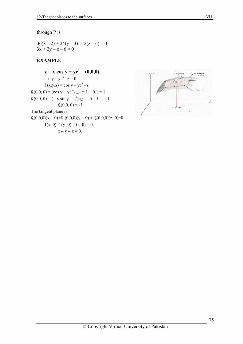
12-Tangent planes to the surfaces VU
through P is 36(x – 2) + 24(y – 3) –12(z – 6) = 0 x + 2y – z – 6 = 0
XAMPLE
3 E
z = x cos y − ye x (0,0,0).
cos y − ye x – z = 0
f (x,y,z) = cos y − yex –
f x (0,0, 0) = (cos y − yex) (0,0) = 1 − 0.1 = 1
f y (0,0, 0) = ( − x sin y − e x ) (0,0) = 0 − 1 = − 1.
f z (0,0, 0) = - 1
The tangent plane is
z
h f
f x (0,0,0)(x − 0)+f y (0,0,0)(y − 0) + f z (0,0,0)(z− 0)=0
1 (x − 0) − 1 (y − 0) − 1 (z − 0) = 0, x − y − z = 0.
© Copyright Virtual University of Pakistan
75

13-Orthogonal surfaces VU
Lecture No -13 Orthogonal Surface
able iables
ere fx means that the function f(x,y,z) is partially differentiate with respect to x And P0) means that the function f(x,y,z) is partially differentiate with respect to x at the
oint P0(x0,y0,z0)
means that the function f(x,y,z) is partially differentiate with respect to y And fy(P0) eans that the function f(x,y,z) is partially differentiate with respect to y at the point 0(x0,y0,z0)
imilarly
means that the function f(x,y,z) is partially differentiate with respect to z And fz(P0) eans that the function f(x,y,z) is partially differentiate with respect to z at the point 0(x0,y0,z0)
XAMPLE
In this Lecture we will study the following topics
• Normal line • Orthogonal Surface • Total differential for function of one vari• Total differential for function of two var
Hfx(
p fy
mP S fzmP E
ind the Equation of the tangent plane and normal of the surface f(x,y,z)= x2+y2+z2-4 at e point P(1,-2,3
ormal line
Let P0 (x0 ,y0 ,z0 ) be any point on the surfaceo P (x 0 ,y 0 ,z 0)
f(x,y,z)=0 If f(x,y,z) is differentiable atthen the normal line at the point P(xo ,y0 0 ,z ) 0 has the equation
x = x 0 +f x (P 0 )t, y = y0+fy(P 0)t, z = z0+fz(P 0 )t
N
Fth ) f(x,y,z) = x
2 +y2+z2 − 14P (1, − 2, 3).
f x = 2x, f y = 2y, fz = 2z f x (p0) = 2, f y (P 0 ) = − 4, fz (P0
) = 6
Equation of the tangent p lane to the surface at P is
© Copyright Virtual University of Pakistan
76

13-Orthogonal surfaces VU
EXAMPLE Find the equation of the tangent plane and normal plane Equations of Tangent Plane to the surface through P is
xample
E
x − 2y + 3z − 14 = 0
Equations of the normal line of the
surface through P are
x − 1
2
2(x − 1) − 4 (y + 2) + 6 (z − 3) = 0
= y + 2
− 4 =
z − 3
6
x − 1
1 =
y + 2
− 2 =
z − 3
3
4x 2−y2 + 3z
2 = 10 P (2, − 3,1)
f(x,y,z) = 4x 2 − y
2 + 3z 2 − 10
fx = 8x, fy = − 2y, fz = 6z
fx (P) = 16, fy (P) = 6, fz (P) = 6
Equations of the normal line to the surface through P are x − 2
16(x − 2) + 6 (y+3) + 6 (z − 1) = 0 8x + 3y + 3z = 10
16 = 6y + 3
= 6z − 1
x − 2 8 =
y + 33 =
z − 13
z = 1 2 x 7 y -2
f(x,y,z) = 1 2 x 7 y -2 – z
f x = 7 2 x 6.y -2,
f y = - x 7.y -3, fz = -1
f x (2, 4, 4) = 7 2 (2)6 (4) = 896
fy (2, 4, 4) = − (2)7 (4)-3 = − 2fz (2, 4, 4) =-1
Equation of Tangent at (2, 4, 4) is given byfx (2,4,4)(x −2)+ fy (2,4,4)(y−4)+ fz (2,4,4)(z−4) = 0
896 (x − 2) + (− 2) (y− 4) − (z − 4) = 0896x − 2y − z − 1788 = 0
The normal line has equations = 2 +x
© Copyright Virtual University of Pakistan
77f x (2,4,4) t, y = 4 +f y (2,4,4) t, z = 4+fz(2,4,4)t
x = 2 + 896t, y = 4 − 2t, z = 4 − t

13-Orthogonal surfaces VU
EXAMPLE
how that given two surfaces are orthogonal or not
ince they satisfied the condition of orthogonality so they are orthogonal.
ifferentials of a functions
S
S D
2 + y2 + z − 16 (1) (x,y,z) = x2 + y2 − 638 (2) dding (1) and (2)
2 + y2 = 634
f(x,y,z) = xgA
x , z = 14 (3)
= 2x, fy = 2y fz = 1 x = 2x, gy = 2y gz = − 63 gx + fygy + fzgz 4 (x2 + y2) − 63 using (3) gx + fy gy + fzgz
4
fxgfx=fx
=⎝⎜⎛
⎠⎟⎞63
4 − 63 = 0
SURFACES ORTHOGONAL
l
Said They are to intersect ort
common to them.
hogonally
at every point
ONDITION FOR
Two surfaces
C ORTHOGONAL SURFACES
are said to be orthogonal at a point of their intersection if their normals a if they are orthogonal
et (x, y, z) be any point o
t that point are orthogonal.
L f intersection of
f (x, y, z) = 0---- (1)
D nand g (x, y, z) = 0 -----(2)
rection ratios of a li e normal to (1) are , fy , ffi x z
x, g y , g z
he two normal lines are orthogonal if and only iT
© Copyright Virtual University of Pakistan
78
f
f x g x + f y g y + fzgz = 0
Similarly, direction rations of a line normal to (2)are g
For a function y = f(x)
dy = f /
(x) d xis called the differential of functions f(x)
d x the differential of x is the same as
the actual change in x
i.e. dx = ∇ x where as dy thedifferential of y is the approximate change in the
value of the functions
w hich
is different from the actual change ∇y in the value of the functions.

13-Orthogonal surfaces VU
Distinction betw
een the incrementn ∆y and the differential dy
Approximation to the curve
If f is differentiable at x , then the at x is a reasonably good approximation
near x0. Since the tangent line passes
0
tangent line to the curve y = f(x) 0 to the curve y = f(x) for value of x
through the point (x0, f(x0)) and has
EXAMPLE
its equation isy − f (x0) =
y = f(x
/ f(x0)(x − x0) or 0 ) + f/(x0) (x − x0)
slope f/(x0 the point-slope form o), f
f(x) = x x = 4 and dx =∆x = 3 y = 3
∆ y = x + ∆x − x = 7 − 4 ≈ .65
If y = x , then dy dx = 1
2 x so dy =1
2 x dx
= 1 2 x
(3) = 3 4 = .75
© Copyright Virtual University of Pakistan
79

13-Orthogonal surfaces VU
EXAMPLE
XAMPLE
E
Using differentials approximation
for the value of cos 61 °.Let y = cosx and x = 6 0°then dx = 61° − 60° = 1°
∆y ≈ dy = − sinx dx = − sin60° (1°)
= 3
2
⎝⎜⎛
⎠⎞1
180 π
Now y = cos x y+∆ y = cos (x+∆x) = cos (x+dx)
= cos (60°+1°)=cos61° cos61° = y+ ∆ y = cosx + ∆y
≈ cos60° − 3
2 ⎝⎜⎛
⎠⎟⎞1
180 π
cos61 ° ≈ 1 2 −
32
⎝⎜⎛
⎠⎟⎞1
180 π
= 0.5 − 0.01511 = 0.48489 cos61° ≈ 0.48489
of the box is 8.5 inches with
±
0.3 inches.
Let x and h be the width and the height of the box respectively, then its volume
V is given by V = x2h
a possible error of box with a square base has its hei ght twice is width. If the
idth
Since h = 2x, so (1) take the form V = 2x3
dV = 6x2 dx Since x = 8.5, dx = ±0.3, so
A
w
putting these values in (2), we have
dV = 6 (8.5) 2 (±0.3) = ± 130.05 This shows that the possible error in the
volume of the box is ±130.05. TOTAL DIFFERENTIAL
e move from (x0 , y0 ) to a poin If w
© Copyright Virtual University of Pakistan
80
t resulting differential in f is
df = fx (x 0 , y 0) dx + fy (x0, y0) dy
This change in the linearization of
(x0 + dx, y0 + dy) nearby, the

13-Orthogonal surfaces VU
EXAMPLE Which is exact Change
XAMPLE
E
Area = xy = 10, y = 8 Area = 80 = 10.03 y = 8.02 Area = 80.4406 xact Change in area = 80.4406 − 80
= 0.4406
XACT CHANGE
f is called the total differential o
E
xxE
f f.
rectanA gular plate expands in such 0 to 10.03 and its breadth changes from 8 to 8.02.
Let x and y the length and
1
breadth of the rectangle respectively, th en its area is
A = xy dA = A x dx + A y dy = ydx + xdy
By the given conditions x = 10, dx = 0.03, y = 8, dy = 0.02.
dA = 8(0.03) + 10(0.02) = 0.44
a way that its length changes from
proximately
. V = xyz
dV = V xd x + Vydy + Vzdx
The volume of a rectangular parallelepipe
dV = yzdx + xzdy + zydz (1)
d is given by the formula V = xyz. If this solid is compressed from above so that z is decreased by 2% while x and y each is increased by 0.75% ap
d x = 100 0.75
x, dy = 100 0.75
y, dz= − 1002
z
Putting these values in (1), we have
dV = 0.75 100 xyz+
0.75 100 xyz −
2100 xyz
= − 0.5 100 xyz = −
0.5100 V
This shows that there is 0.5 % decrease in the volume.
© Copyright Virtual University of Pakistan
81

13-Orthogonal surfaces VU
EXAMPLE
d∆=12 4 sin 30°(0.1)+
12 9 sin 30°(0.08)
+ 21
36cos 30° ⎝⎜
⎠⎟3600
⎛ ⎞π
d∆=2⎝⎜⎛
⎠⎟⎞1
2 (0.1)+12
⎝⎜⎛
⎠⎟⎞1
2 (0.08)
+18 ⎝⎜⎛
⎠⎟⎞3
2 ⎝⎜⎛
⎠⎟⎞3.14
3600 = 0.293
% change in area = 0.293
∆ × 100
= 0.293
9 × 10 = 3.25%
By the given conditions a = 9, b = 4, C = 30°,
da = 9.1 − 9 = 0.1, db = 4.08 − 4 = 0.08
dC = 30°3′ − 3′ = ⎝⎜⎛
⎠⎟⎞3
60°
= 3
60 × π
180 radians
Putting these values in (1), we have
∆ = 12 ab sin C
d∆ = ∂∂a
⎝⎜⎛
⎠⎟⎞1
2 ab sin C da + ∂
∂b ⎝⎜⎛
⎠⎟⎞1
2 ab sin C db
+ ∂
∂C ⎝⎜⎛
⎠⎟⎞1
2 ab sin C dC
d∆ = 12 b sin Cda +
12 a sin C db
+ 12 ab cos CdC
A formula for the area ∆ of a triangle is
∆ = 12 ab sin C. Approximately what error is
made in computing ∆ if a is taken to be 9.1 instead of 9, b is taken to be 4.08 instead of 4 and C is taken to be 30°3/ instead of 30°.
© Copyright Virtual University of Pakistan
82

14-Extrema of functions of two variables VU
© Copyright Virtual University of Pakistan 83
Lecture No -14 Extrema of Functions of Two Variables In this lecture we shall fined the techniques for finding the highest and lowest points on the graph of a function or , equivalently, the largest and smallest values of the function. The graph of many functions form hills and valleys. The tops of the hills are relative
axima and the bottom of the valleys are called relative minima. Just as the top of a hill n the earth’s terrain need not be the highest point on the earth , so a relative maximum
need not be the highest point on the entire graph . Absolute maximum
mo
t some point (x0,y0) of its at (x0,y0) and of radius r
The function f is said to have a relative (local ) maximum adomain D if there exists an open disc K centered With such that
f of two variables on a subset
of R 2
value on D if there is some point
f ( x 0 , y 0 ) > f ( x , y ) for all ( x , y ) ∈ D
f ( x 0 , y 0 ) is the absolute maximum
x ( 0, y ) of 0 such that D value of f on D A function is said to have an D absolute (global) maximum
In such a case
Relative extremum and absolute extremum
If f has a relative maximum or a relativerelative extremum at (x 0 ,y 0 ), and if f has an
(x0 ,y 0 ), then we say that f has an absolute
minimum at (x0, y 0), then we say that f has a
absolute maximum or absolute minimum at
extremum at (x 0,y0 ).
Absolute minimum
A function f of two variables on a subset D of R2
minimum value on D if there is some point
( ) ( ) for all ( ) In such a case ( ) is the absolute minimum value of f on D .f x0 , y 0
is said to have an absolute (global)
(x0, y0 D ) of such that
f x 0 , y0 ≤ f x, y x, y ∈ D.
Relative (lo
R elative (local) maximum
K ={( x , y ) ∈ R 2 : (x − x0)2 + ( y − y0)2 < r2 } K ∈ D
f(x0, y 0) ≥ f (x, y) for all (x, y )
cal) minimum

14-Extrema of functions of two variables VU
The function f is said to have a relative (local) minimum at some point
( x 0 , y 0 ) of D if there exists an open disc centred at (x 0, y0) and of radius K
xtreme Value Theorem
r K ⊂ D with such that
f ( x0, y 0 ) ≤ f (x, y) for all (x, y) ∈ K.
E
f (x, y) is continuous on a closed and bounded set R, then f has both n absolute maximum and on absolute minimum on R .
emarks
Ifa R
any of the conditions the Extreme Value Theorem fail to hold, then there is no uarantee that an absolute maximum or absolute minimum exists on the region R. hus, a discontinuous function on a closed and bounded set need not have any absolute xtrema, and a continuous function on a set that is not closed and bounded also need not ave any absolute extrema.
xtreme values or extrema of f
IfgTeh E
he maximum and minimum values of f are referred to as extreme values of extrema of f et a function f of two variables be defined on an open disc
Suppose
K
T.L If f has relative extrema at (x0,y0),then
x, y x − x0)2 y − y0 = {( ): ( + ( < )2 r2 }.
f x ( x0, y0
fy( x 0 , y0) and ) both exist on K
f x (x 0, y0 ) = 0 = fy(x0, y0).
© Copyright Virtual University of Pakistan
84

14-Extrema of functions of two variables VU
Saddle Point
A differentiable function f(x, y) has a saddle has a saddle point (a, b) if in every
open disk centered at (a, b) there are domain points (x, y) where f (x, y) > f (a, b) and omain points (x, y) where f (x, y) < f (a, b). The corresponding point (a, b, f (a, b)) on d
the surface z = f (x, y) is called a saddle point of the surface
Remarks Thus, the y points where a function f(x,y) can assume extreme values are critical
undary points. As with differentiable functions if a single variable, not every e might
onlpoints and bocritical point gives rise to o a local extremum. A differentiable function of a singlvariable might have a point of inflection. A differentiable function of two variable have a saddle point. EXAMPLE Fine the critical points of the given function
Substituting the value of x from (2) into (1),we have
4ya2 − ay = 0
y(y3 − a3) = 0 y= 0, y= a
and so x = 0, x= a.
The critical points are (0, 0) and (a, a).
3 3
x 2 y
For critical points fx = fy = 0. Therefore, x2 − ay = 0 (1)
d ax − y2 = 0 (2)
f (x, y) = x + y − 3axy, a > 0. fx, f y exist at all points of the domain of f.
f = 3x − 3ay, f = 3y2 − 3ax
an
© Copyright Virtual University of Pakistan
85

14-Extrema of functions of two variables VU
Overview of lecture # 14 Topic Article # page # Extrema of Functions of Two Variables 16.9 833 Absolute maximum 16.9.1 833
nimum 16.9.2 833
xtreme Value Theorem 16.9.3 834
Absolute m
a
E
Exercise set Q#1,3,5,7,9,11,13,15,17 841 Book CALCULUS by HOWARD ANTON
© Copyright Virtual University of Pakistan
86

15-Examples VU
Lecture No - 15 Example
XAMPLE E
xample
E
f ( x , y) = x + 2 y2
x f x ( x , y ) = x 2 + y 2
f
y (x , y) = y
x 2 + y 2
the domain of except at the origin which is fThe partial derivatives exist at all points off f . Thus (0, 0) is a criticalin the d ain oom point of f
fNow x(x, y) = 0 only if x = 0 andf y
( x , y ) = 0 only if y = 0
The only critical point is (0,0) and f(0,0)=0
Since f (x , y ) ≥ 0 for all (x, y), f (0, 0) = 0 is the absolute minimum value of f .
z = f(x, y) = x 2 + y2 (Paraboloid)fx (x, y) = 2x, f y (x, y) = 2ywhen fx (x, y) = 0, fy (x, y) = 0we ha ve (0, 0) as critical point.
© Copyright Virtual University of Pakistan
87

15-Examples VU
EXAMPLE
XAMPLE
E
XAMPLE
E
The point (0,0) is critical point of f because the partial derivatives do not both exist. It is evident geometrically that fx(0,.0) does not exist because the trace of the cone in the plane y=0 has a corner at the origin.
f(x, y) = x2 + y2 x =
x
x2 + y2 fy =
y
x2 + y2
z = g(x, y) = 1 − x, y) = − 2x, g y (x, y) =
2 − y2 (Paraboloid)
g x (x − 2ygx (x, y) = 0 , g y (x, y) = 0
we h a ve (0, 0) as critical point.
z = h(x, y)=y2− x2 (Hyperbolic paraboloid)
hx (x, y) = − 2x, h
when
f
y (x, y) = 2ywhen hx (x, y) = 0 , h y (x, y) = 0we ha ve ( 0, 0) as critical point.
The fact that f x (0,0) does not exist canalso be seen algebraically by noting that fx (0,0) can be interpreted as thederivative with respect to x of the function
f (x, 0) = x2 + 0 = |x| at x = 0.
© Copyright Virtual University of Pakistan
88

15-Examples VU
The Second Partial Derivative Test
EMARKS
R
a function f of two variables has an absolute extremum (either an absolute maximum or n absolute minimum) at an interior point of its domain, then this extremum occurs at a
l point. EXAMPLE
Ifacritica
differentiable at x = 0, so But |x| is not f x(0,0) does not exist. Similarly, (0,0) does not exist. The function ff y has a relative minimum at the critical
point (0,0).
et L f be a function of two variables with continuous second order partial derivatives
in some circle centered at a critical point (x0, y0), and let
D = f xx (x0 , y 0) fyy(x0, y0) − f 2xy(x0, y0)
fxx 0,y0(a) If D > 0 and (x ) > 0 , then f has a 0,y0 relative minimum at (x ).
(b) If D > 0 and fxx(x0,y0) < 0 , then f has arelative maximumat (x0,y0).
(c) If D < 0 , then f has a saddle point at (x0,y 0 ).
(d) If D = 0 , then no conclusion can bedrawn.
f(x,y) = 2x 2 − 4x + xy2 − 1f x (x, y) = 4x− 4 + y2, fxx (x, y) = 4f y (x, y) = 2xy, fyy (x, y) = 2x
f xy (x, y) = fyx (x, y) = 2y
al points, we set the first partial derivatives equal to zero. Then 4x − 4 + y2 = 0 (1)
For critic
and 2xy = 0 (2) we have x = 0 or y = 0
x = 0, then from (1), y = ± 2. y = 0, then from (1), x = 1.
Thus the critical points are (1,0), (0, 2), (0,
− 2).
© Copyright Virtual University of Pakistan
89

15-Examples VU
We check the nature of each point.
f xx(1,0) = 4,
f yy (1, 0) = 2,
f xy (1, 0) = 0
D= f xx (1, 0).f yy (1, 0
= 8 > 0 EXAMPLE
) - [f xy (1, 0)] 2
and f xx (1, 0) is positive. Thus f has a
relative minimum at (1, 0).
f xx (0, 2) = 4,f yy (0, 2) = 0,f xy (0, 2) = 4
D= fxx (0, 2).fyy (0, 2) - [fxy (0, 2)]2 = − 16 < 0. Therefore, f has a saddle point at (0,2).
f xx(0,−2) = 4,f yy (0,−2) = 0,fxy (0,−2) = −4
D= fxx (0, − 2).fyy (0, − 2) - [fxy (0, − 2)]2
= − 16 < 0.
f(x,y) = e-(x2+y2+2x)
f x (x, y)=−2 (x+1)e-(x2+y2+2x),
f y(x, y) = − 2ye-(x2+y2+2x)
For critical pointsfx (x,y) = 0, x + 1 = 0, x = − 1 and
fy (x, y) = 0, y = 0Hence critical point is (−1,0).
f xx (x,y) = [( − 2x − 2) 2 − 2]e
-(x2+y2+2x)
f xx ( − 1, 0) = - , f yy (x,y) = [4y
2 − 2]e -(x2+y2+2x)
f yy ( − 1, 0) = -
f xy (x,y) = − 2y ( − 2x − 2)e -(x2+y2+2x)
f xy ( − 1, 0) = 0
D = f xx ( − 1,0) f yy( − 1, 0) − f 2xy ( − 1, 0)
= (-2e ) (-2e ) > 0
This shows that f is maximum at ( − 1, 0).
2).Therefore, f has a saddle point at (0,−
© Copyright Virtual University of Pakistan
90

15-Examples VU
EXAMPLE f(x,y) = 2x4 + y2 − x2 − 2y
f x (x, y) = 8x 3 − 2x, fy(x, y) = 2y − 2 f xx (x, y) = 24x 2 − 2, f yy(x,y) = 2,
fxy (x, y) = 0 For critical points
f (x, y) = 0, x
2x (4x2 − 1) = 0, x = 0,1/2,-1/2 f y (x, y) = 0,
2y − 2 = 0, y = 1
Solving above equation we have the critical
points (0,1), ⎝ ⎜ ⎛
⎠⎟⎞
− 12 , 1⎝⎜⎛
⎠⎟⎞1
2 , 1 .f xx (0,1) = − 2, fyy (0, 1) = 2,f xy (0, 1) = 0 D = fx(0, 1) fyy (0, 1) − f2
xy (0, 1)= ( − 2)(2) − 0 = −4 < 0This shows that (0, 1) is a saddle point.
f xx ⎝ ⎜ ⎛
⎠
⎞ 1
2 , 1 = 4, f yy =
⎝ ⎜ ⎛
⎠
⎞ 1
2 , 1 = 2
f xy ⎝ ⎜ ⎛
⎠
⎞ 1
2 , 1 = 0
D = f xx ⎝ ⎜ ⎛
⎠
⎞ 1
2 , 1 f yy
⎝ ⎜ ⎛
⎠
⎞ 1
2 , 1
− f 2xy
⎝ ⎜ ⎛
⎠
⎞ − 1
2 , 1
= (4) (2) − 0 = 8 > 0
f xx ⎝ ⎜ ⎛
⎠
⎞ 1
2 , 1 = 4 > 0, so f is minimum at
⎝ ⎜ ⎛
⎠
⎞ 1
2 , 1 .
© Copyright Virtual University of Pakistan
91

15-Examples VU
Example
ver view
Locate all relative extrema and
3
Solving ( 1 ) and (2 ), we have the
critical points (0,0), (1, 1),(− 1, − 1).
Now ff yy − 2
f xy
D = f
(x, y) = 12y , f yy (0,0) = 0
(x, y) = 4, f xy (0, 0) = 4
xx (0,0) f y (0,0) − f 2 xy (0,0)
= (0) (0) − (4) 2 = - 16 < 0
This shows that (0,0) is the saddle point.
f xx (x, y) = − 12x2 , f xx (1,1) = − 12 < 0f yy (x,y) = − 12y2 , f y (1,1) = − 12f xy (x, y) = 4, fxy (1,1) = 4D = fxx (1,1) fyy (1,1) − f 2 xy (1, 1) = ( − 12) (− 12) − (4) 2 = 128 > 0This shows that f has relative maximum at (1,1).
f xx (x,y) = − 12x 2 , f xx ( − 1, − 1) = − 12 < 0
f y (x, y) = − 2y 2 , f y ( − 1, − 1) = − 12
(x, y) = 4, f xy ( − 1, f xy − 1) = 4
xx ( − 1, D=f − 1) f yy ( − 1, − 1) − f 2
xy( − 1, − 1)
= ( − 12) ( − 12) − (4) 2 = 128 > 0
This shows that f has relative maximum − 1).
( − 1,
xx (x, y) = − 12x 2 ,
f xx (0, 0) = 0
saddle points of f (x, y) = 4xy − x4 − y4.
fx(x, y) = 4y − 4x3, fy (x, y) = 4x − 4yFor critical points
fx (x, y) = 0 4y − 4x3 = 0 (1) y = x3
fy (x, y) = 0 4x − 4y3 = 0 (2) x = y3
O of lecture # 15 Book Calculus by HOWARD ANTON
opic # Article # Page # xample 3 836 raph of f(x,y) 16.9.4 836 he Second Partial Derivative Test 16.9.5 836 xample 5 837
TEGTE
© Copyright Virtual University of Pakistan
92

16-Extreme valued theorem VU
Lecture No -16 Extreme Valued Theorem
EXTREME VALUED THEOREM
If the function f is continuous on the closed interval [a, b], then f has an absolute maximum value and an absolute minimum value on [a, b] Remarks An absolute extrem st be either a relative extremum a necessary condition
at C be a critical point, we may determ minimum value of a continuous f
. Find the critical points of f on [a, b] and the function values at these critical.
. Find the values of f (a) and f (b).
. The largest and the smallest of the above calculated values are the absolute maximum alue and the absolute minimum value respectively xample
um of a function on a closed interval mu or a function value at an end point of the interval. Since
for a function to have a relative extremum at a point C is thine the absolute maximum value and the absoluteunction f on a closed interval [a, b] by the following procedure.
123v E
ind the absolute extrema of
ince f is continuous on [-2,1/2], the extreme value theorem is applicable. For this
f /(x) =3 x2+2x-1
his shows th ly critical numbers of f will e the values of x for which f (x)=0. .
F f(x)= x3+ x2-x+1 on [-2,1/2] S
at f(x) exists for all real numbers, and so the onTb
Setting f
/ (x) = 0, we have
− 1) (x + 1) = 0 which we obtain
− 1 an
(3x from
d x = 1 3
− 1 and 13
x =
,
The critical points of f are
(-2, 1 2 ) We find the function
closed interval
points of the interval, which are given below.
and each of these points is in the given values at the critical points and at the end
f( − 2) = − 1, f ( − 1) = 2,
f ⎝
⎛
⎠
⎞ 1 3
= 27 22 , f
⎝ ⎜ ⎛
⎠
⎞ 1 2
= 8 7
The ab s m m -2, 2olute aximu value of f on (1
) is therefore
2, which rs at occu − 1, and the absolute min. value of f on
( - 2, 1 2
© Copyright Virtual University of Pakistan
93
) is − 1, wh cc th end point ich o urs at e left − 2.
Find the absolute extrema of −

16-Extreme valued theorem VU
so that the absolute extrema occur either at 2 or at one of the end points of the interval. The function values at these points are given below.
f(1) = 1 , f(2) = 0, f(5)=
the absolute minimum value of f on [1,5] isFrom these values we conclude that occurring at 2, and the absolute maximu
0, 3
h mum is 0, assumed at
to Find the Absolute Extrema of a Continuous Function f of Two Variables on
m value of f on [1, 5] is 9 ,occurring at 5. Tx = 0.
e absolute maximum value is 9 assumed at x = 3; the absolute mini
Howa Closed and Bounded Region R.
itical points of f that lie in the interior of R. etp 2.
Find all boundary points at which the absolute extrema can occur, tep 3.
Evaluate f(x,y) at the points obtained in the previous steps. The largest of these alues is the absolute maximum and the smallest the absolute minimum.
Find the absolute maximum and minimum value of
f (x) = (x 2) 2/3 on [1, 5].
Since f is continuous on [1. 5], the extreme- value t theorem is applicable.
etDifferentiating f with respect to x, we g
f / (x) =
2 3 ( x − 2 )
1/3
There is no value of x for which f (x) = 0. However, since f (x) does not exist at 2, we conclude that 2 is a critical point of f,
/ /
39
Find the absolute extrema of on [− 2, 3].
h
h(x) = x 2/3
Step 1. Find the crS S v
(x) = 3 / 2
x = - 1/3 21/33x
/
h (x) has no zeros but is undefined at x = 0.
he values of h at this one critical poin T t and x = 3 are
1/3
and at the endpoints x =− 2 h(0) = 0 h (− 2) = (− 2)2/3 = 41/3
h(3) = (3)2/3 = 91/3.
© Copyright Virtual University of Pakistan
94

16-Extreme valued theorem VU
f(x,y) = 2 + 2x +2y-x2-y2 n the triangular plate in the first quadrant bounded by the lines x=0,y=0,y=9-x ince f is a differentiable, the only places where f can assume these values are points side the triangle having vertices at O(0,0), A(9,0)and B(0,9) where fx = fy=0 and points
f boundary.
OSino O
or interior points:F We have fx=2-2x=0 and fy=2-2y=0
ielding the single point (1,1)
or boundary points we take take the triangle one side at time : 1. On the segment OA, y=0
U(x) = f(x, 0)=2+2x-x2
ay be regarded as function of x defined on the closed interval 0≤x≤9 Its extreme alues may occur at the endpoints x=0 and x=9 which corresponds to points (0, 0) and , 0) and U(x) has critical point where
n x=1
V(y)=f(0,y)= 2+2y-y
y F
mv(9
U/(x) = 2-2x=0 TheOn the segment OB, x=0 and
2
Using symmetry of function f, possible points are (0,0 ),(0,9) and (0,1)
B ( 0, 9)
.(9/2,9/2) x = 0
y = 9 - x
0
. - x, we have
.(1,1)
y = A( 9,0)
3. T he interior points of AB With y = 9
f (x , y) = 2+2x+2(9 - x) – x2–(9- x)(x) = f(x, 9 - x) = - 61 +18x
2
– 2x2W Setting w′(x)= 18 -4x = 0, x = 9/2.
this value of x, y = 9
At – 9/2
herefore we have (92, 9
2 ) as a critical point.
T
(x, y) (0,0)
(9,0) (1, 0)
⎝⎜⎛
⎠⎟⎞
92 ,
92
f(x,y)
2
−61 3 −
412
© Copyright Virtual University of Pakistan
95
(x, y)
(0, 9) (0,1) (1,1)
f(x,y)
− 61 3 4

16-Extreme valued theorem VU
aximum is 4 which f assumes at the point (1,1) The absolute minimum is 1 which f assumes at the points (0, 9) and (9,0)
XAMPLE
The absolute m-6 E
ind the absolute maximum and the absolute minimum values of f(x,y)=3xy-6x-3y+7
n the closed triangular region r with the vertices (0,0), (3,0) and (0,5) .
ine the extrema might occur.
simplifies to a function of the single variable x,
ints because u/(6)=-6 is non zero for all x . Thus, the extreme values of u(x) occur at the endpoints x = 0 and x=3 , which corresponds to the
ii) The line segment between the (0,0) and (0,5)
n this line segment we have x=0 ,so single variable y,
5
his function has no critical points because v/(y)=-3 is non zero for all y.Thus ,the xtreme values of v(y) occur at the endpoints y = 0 and y=5 which correspond to the point ,0) and (0,5) or R
iii) The line segment between (3,0) and (0,5)
f(x, y) = 3xy
F o
− 6x − 3y + 7fx(x, y) − 6, fy(x, y) = 3x−3 For cri points fx (x, y) = 0 3y − 6 = 0 y = 2 fy(x, y) = 0 3x − 3 = 0
= 3y tical
x = 1 Thus, (1, 2) is the only critical point in the interior of R. Next, we want to determlocation of the points on the boundary of R at which the absoluteThe oseparately.
boundary extrema might ccur. The boundary each of which we shall treat
i)The line segment between (0, 0) and (3, 0):
ment we have y=0 so (1) On this line seg
This fu o
u (x)=f(x, 0) = − 6x +
nction has no critical p
points (0, 0) and (3,0) on R
7, 0 < x < 3
v(y) = f (0, y) = − 3y + 7, 0 < y <
O
Te(0
© Copyright Virtual University of Pakistan
96

16-Extreme valued theorem VU
© Copyright Virtual University of Pakistan 97
In the XY- plan , an equation for the line segment
(1) simplifies to a function of the single variable x,
e values of w occur points
rrespond to f R, and from (6) the critical point corresponds to [7/5,8/3]
Finally, table list the values of f(x,y) at the interior critical point and at the points on the boundary where an absolute extremum can occur. From the table we conclude that the bsolute maximum value of f is f(0,0)=7 and the absolute minimum values is f(3,0)=-11.
6.9 Q #26,27,28,29.
Lecture No -17 Examples
(x, y)
(0, 0)
(3, 0)
(0, 5) ⎝
⎜⎛
⎠⎟⎞7
5
so This shows that x =7/5 is the only critical point of w. Thus, the extremeither at the critical point x=7/5 or at the endpoints x=0 and x=3.The endco the points (0, 5) and (3, 0) o
, 83
(1, 2)
f(x,y)
7
− 11
− 8 −
95
1
y = − 5
3 x + 5, 0 < x < 3
(x) = f (x, − 5
3 x + 5)
= − 5x 2 + 14x − 8, 0 <
w
a OVER VIEW: Maxima and Minima of functions of two variables. Page # 833Exercise: 1
x < 3
0x + 14 = 0
w ′ (x) = − 10 x + 14
w ′ (x) = 0
1 x = 5
7

17-Examples VU
EXAMPLE Fin ,y)=xy-x-3y on the closed triangular region R with vertices (0, 0), (0, 4), and (5, 0).
Thus, (3, 1) is the only critical point in the interior of R. Next, we want to determine the
which the absolute extrema might occur. The boundary of R consists of three line segments, each of which we shall treat
The function has no critical points because the u/(x)=-1 is non zero for all x.Thus,the exteme values of u(x) occure at the endpoints x=0 and x=5 , which corresponds to the points (0,0) and (5,0) of R. ii) The line segment between (0,0) and (0,4)
ints because v/ (y)= -3 is nonzero for all y. Thus, the
i) The line segment between (5,0) and (0,4) the xy-plan, an equation is
(1) simplifies to a function of the single variable x,
(x) = f (x, − 45
d the absolute maximum and minimum values of f(x
© Copyright Virtual University of Pakistan 98
location of the points on the boundary of R at
separately. (i) The line segment between (0, 0) and (5,0) On this line segment we have y = 0, so (1) simplifies to a function of the single variable x,
On this line segment we have x = 0, so (1) simplifies to a f nction of the single variable y,
u
This function has no critical poextreme values of v(y) occur at the endpoints y =0 and y=4 ,which correspond to the point
. (0,0) and (0,4) or R iiIn so
w x + 4)
− 45= x2 +
35 x + 12, 0 < x < 5
′(x) = − 85w x +
35 , w′(x) = 0
= 38x
f (x,y) = xy − x − 3y (1)
(x, y) = y − 1, f
f x y (x, y) = x −
For critical points
f x (x, y) = 0, y
− 1 = 0
y = 1 (2)
f
3
y (x, y) = 0, 3x − 3 = 0
x = 3 (3)
u (x) = f (x, 0) = − - x, 0 <
x < 5 (4)
v(y) = f (0, y) = − 3y, 0 < y < 4. (5)
= − 4
5 x+ 4, 0 < x < 5 (6) y

17-Examples VU
38
This shows that x = is the only critical point of w. Thus, the extreme values of w occur
ritical point x = 38
either at the c or at the endpoints x = 0 and x = 5. The endpoints
ponds correspond to the points (0, 4) and (5, 0) of R, and from (6) the critical point corres
to 3 37,⎡ ⎤ 8 10⎢ ⎥⎣ ⎦
Finally, from the table below, we conclude that the absolute maximum value of f is f (0,0) = 0 and the absolute minimum value is
3 37,8 10
f ⎛ ⎞⎜ ⎟⎝ ⎠
=-807/80
Example Find three positive numbers whose sum is 48 and such that their product is as large as
ossible pLet x,y and z be the required numbers, then we have to maximize the product
, y
z = 48
f(x,y)=xy(48-x-y) Since fx=48y-2xy-y2 f =48x-2xy-x2
solving fx =0 , fy=0 we get x=16, y=16, z=16 Since x+y+z=48 For x = 16, y = 16 we have z = 16 since x + y +
16, 16, 16. Thus, the required numbers are Example Find three positive numbers whose sum is 27 and suchmall as possible
that the sum of their squares is as
(x, y)
(0,0)
(5,0)
(0, 4) ⎝
⎜⎛
⎠⎟⎞3
8 , 3710
(3, 1)
f(x,y)
0
− 5
− 4 −
80780
− 3
(x,y ) = - 2y, f xx (16, 16 ) = - 32 < 0
(x, y ) = 48 - 2x - 2y, f xy (16, 16 ) = - 16 f xx
f xy
f yy (x, y ) = - 2x, f yy (16, 16 ) = - 32
D=f xx (16,16 )f y7y (16,16 ) − f 2
xy (16,16 ) = ( − 32) ( − 32) − (16)
2 = 768 > 0
s
we have to Let x, y, z be the required numbers, then
f(x,y) = x 2 + y
2 + z 2
= x 2 + y
2 + (27 − x − y) 2
Since x+y+z = 27 f x = 4x+2y − 54, f y = 2x+4y − 54, f xx = 4, f yy = 4, f xy = 2
© Copyright Virtual University of Pakistan
99
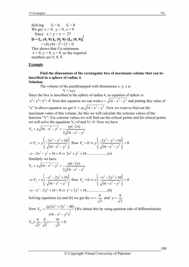
17-Examples VU
Example
be
Solution: Th f the parallelepiped with dimensions x, y, z is
V = xyz
= 4 from this equation we can write
Find the dimensions of the rectangular box of maximum volume that caninscribed in a sphere of radius 4.
e volume o
Since the box is inscribed in the sphere of radius 4, so equation of sphere is x2+ y2+ z2 2 2 216z x y= − − and putting this value of
“z” in above equation we get 2 216 x y− − .Now we want to find out the V xy=maximum value of this volume, for this we will calculate the extreme values of the
e critical points and for critical points olve the equations Vx=0 and Vy=0 .Now we have
function “V”. For extreme values we will find out thwe will s
2 2 ( 2 )6 xy xx −2 2
12 16
xV y yx y
= − − +
2 2 2 2
2 2 2 2
2 2 2 2
2 16 2 160 016 16
2 16 0 2 16......................( )
x xx y x yV y Now V y
x y x y
x y x y a
−
⎧ ⎫ ⎧ ⎫− − + − − +⎪ ⎪ ⎪ ⎪⇒ = = ⇒ =⎨ ⎬ ⎨ ⎬− − − −⎪ ⎪ ⎪ ⎪⎩ ⎭ ⎩ ⎭
⇒ − − + = ⇒ + =
imilarly we have
−
S 2 2 ( 2 )16y
xy yV x x y −= − − +
2 22 16 x y− −
2 2 2 2
2
2 16 2 160 0
0 2 16......................( )
x y x yNow V x
x y b
⎧ ⎫ ⎧ ⎫− − + − − +⎪ ⎪ ⎪= ⇒ =⎬ ⎨ ⎬
= ⇒ + =
2 2 2 2
2 2
16 16
2 16
y yx y x y
x y
− − − −⎪ ⎪ ⎪ ⎪⎩ ⎭ ⎩ ⎭− − + 2
V x ⎪⇒ = ⎨
⇒
Solving equations (a) and (b) we get the 4 43 3
x and y= =
Now 2 2
32 2 2
(2 3 48)
(16 )xx
xy x yVx y
+ −=
− −(We obtain this by using quotient rule of differentiation)
4 4 16( , )3 3 3xxV = − ≺ 0
Solving
f x = 0, f y = 0
W e get x = 9, y = 9,
z = 9
Since x + y + z = 27
D = f xx (9, 9) f yy (9, 9) − [f xy (9, 9)] 2
2
= (4) (4) − 2 =12 > 0
This shows that f is minimum
x = 9, y = 9, z = 9, so the required
numbers are 9, 9, 9.
© Copyright Virtual University of Pakistan
100

17-Examples VU
Also we have to calculate 2 2
32 2 2
(3 2 48)
(16 )yy
xy x yVx y
+ −=
− −and 4 4 16( , )
3 3 3yyV = − ≺ 0 Also note
at 4 4 8( , )3 3 3xyV = −th Now as we have the formula for the second order partial
is ) 2. (xx yy xyf f f−derivative and putting the values which we calculated above we note
atth 2( , ). ( , ) ( ( , )) 033 3 3 3 3 3yy xyf f− = +
4 4 4 4 4 4 320xxf
has maximum value when
Which shows that the
4 4function V3 3
x and y= = . So the dimension of the
rectangular box are 4 ,= =4 4
3 3 3x y and z = .
Example A closed rectangular box with volume of 16 ft3 is made from two kinds of materials. The top and bottom are made of material costing Rs. 10 per square foot and the sides from material costing Rs.5 per square foot. Find the dimensions of the box so that the cost ofmaterials is minimized
e e length, width, height, and cost of the box respectively. Then it is
C=10(xy+xy)+5(xz+xz)+5(yz+yz)---------------(1)
The volume of the box is given by
Let x, y, z, and C b thcl ar form that e
C=20xy+10(x+y)z
xyz=16----------------------------------(2)
For critical points x = 0C
20y − 160x2 = 0 and Cy = 0
20x − 160y2 = 0
Solving these equations, we have x = 2, y = 2. Thus the critical point
(2, 2).
Putting the value of z from(1), we have
16
(2) in
C = 20xy + 10 (x + y) xy
C = 20 xy + y
160 160 + x
C x =20y - 160
x2 , C y = 20x −
160
y2
is
© Copyright Virtual University of Pakistan
101

17-Examples VU
xx (x, y) = 320x3 C
Cxx (2, 2) = 3208 = 40 > 0
yy (x, y) = 320y3C
Cxx(2,2) Cyy(2,2) – C2
xy(2,2) =(40)(40)-(20)2=1200>0 This shows that S has relative minimum at x = 2 and y = 2. Putting these values in (2), we have z = 4, so when its dimensions are 2 ×2 ×4.
xample
Cyy (2, 2) = 3208 = 40
Cxy (x, y) = 20 Cxy (2, 2) = 20
E
Find the dimensions of the rectangular box of maximum volume that can be
th dimensions x, y, z is
radius 4, so equation of sphere is
inscribed in a sphere of radius a. Solution:
The volume of the parallelepiped wiV = xyz
Since the box is inscribed in the sphere of x2+ y2+ z2= 42 from this equation we can write 2 2 2z a x y= − − and putting this value of
“z” in above equation we get 2 2 2V xy a x y= − − .Now we want to find out the maximum value of this volume, for this we will calculate the extreme values of the function “V”. For extreme values we will find out the critical points and for critical points we will solve the equations V =0 and V =0 .Now we have x y
2 2 2
2 2 22xV y a x y
a x y= − − +
− −
2 2 2 2 2 2
2 2 2
2 20x xx y a x y aV y Now V y
a x y
⎧ ⎫ ⎧ ⎫− − + − − +⎪ ⎪ ⎪ ⎪⇒ = = ⇒⎨ ⎬ ⎨− − ⎪ ⎪2 2 2
2 2 2 2 2
( 2 )
0
2 16 0 2 ......................( )
xy x
a x y
x y x y a a
−
=⎬− −⎩ ⎭
− − + = ⇒ + =
⎪ ⎪⎩ ⎭
⇒Similarly we have
2yV x a= 2 2 ( 2 )xy y−
2 2 22 a x y− −
2 2 2 2 22 20 0y yx y a x y aV x Now V x
⎧ ⎫ ⎧ ⎫− − + − − +⎪ ⎪ ⎪ ⎪⇒ = = ⇒ =⎨ ⎬ ⎨ ⎬ 2
2 2 2
2 2 2 2 2 22 0 ......................( )
a x y
x y a x y a b
− −⎪ ⎪ ⎪ ⎪⎩ ⎭ ⎩ ⎭⇒ − − + = ⇒ + =
Solving equations (a) and (b) we get the
2 2 2
2
x y
a x y
− − +
− −
3 3a ax and y= =
© Copyright Virtual University of Pakistan
102

17-Examples VU
2 2 2
32 2 2 2
(2 3 3 )
( )xx
xy x y aVa x y
+ −=
− −Now (We obtain this by using quotient rule of differentiation)
2
( , )3 3 3xx
a a aV = − ≺ 0
Also we have to calculate 2 2
32 2 2 2
(3 2 3 )
( )yy
2xy x y aVa x y
+ −=
− −and
2
( , )3 3 3yy
a a aV = − Also note
that 2( , )3 3 3xy
a a aV = −
tive is
Now as we have the formula for the second order partial
deriva )2. (xx yy xyf f f− and putting the values which we calculated above we note
that 2
2 20( , ). ( , ) ( ( , ))33 3 3 3 3 3xx yy xy
a a a a a a af f f− = + 0 Which shows that the
function V has maximum value when 3 3
a ax = =and y . So the dimension of the
rectangular box are ,3 3
a3
x y and z= = .
Example: nts o the plane x + y + z t which um value.
Solution: Since we hav 2 2
equation we can writy,z) = (5 – y – z )y2z2
is function. On sim
above equations we get – 10 + 5z = 0 ⇒z = 2 and 10 – 3y – 4 = 0 ⇒y = 2 yy = 10z
yzz(2,2) = 40 − 16 − 48 = − 24 u
a a=
Find the poi = 5 in the first octant af(x,y,z) = xy2z2 has maxim
e f(x,y,z) = xy z and we are given the plane x + y + z = 5 from this e x = 5 – y – z . Thus our function “f’ becomes
f((5 – y – z),y,z) = (5 – y – z )y2z2 Say this function u(y,z) That is u(Now we have to find out extrema of th plification we get u(y,z) = 5 y2z2 – y3z2 – y2z3
On solving
u 2 − 6yz2 − 2z3 uzz = 10y2 − 2y3 − 6y2z uyz = 20yz − 6y2z − 6yz2 at y = 2, z = 2 uyy (2,2) = 40 − 48 − 16 = − 24 < 0
yz (2,2) = 80 − 48 − 48 = − 16
u = 10yz2−3y2z2−2yz3
uz = 10y2z − 2y3z − 3y2z2 = y2z (10 − 2y − 3z)
= 0 0
10 − 3
y = yz2(10 − 3y − 2z)
uy = 0, uz y = 0 , z = y − 2z = 0 10 − 2y − 3z = 0
© Copyright Virtual University of Pakistan
103

17-Examples VU
Example:
the first octant at which f(x,y,z)=xy2z2 has
m value when x = 1 and y = 2. Thus the points where the function
=−y
Find all points of the plane x+y+z=5 in a maximum value.
Hence “f” has maximuhas maximum value is x = 1,y = 2 and z = 2.
fxx2 (5−3x−y) − 3y2 (5−x−5)
f −3x−y)−y2 (5−3x−y) − y (5 − x − y) fyy=2x(5−x−y)(5−x−2y)−2xy(5−x−2y) − 4xy (5 − x − y) fxx (1, 2, 2) = − 24 < 0 fyy (1, 2, 2) = − 16
xy (1, 2, 2) = − 8 fxx fyy − (fxy)2 = (−24)(−16)−(−8)2 = 320 > 0
D = uyy uzz − (uyz)2 = (− 24) (− 24) − (− 16)2 = 576 − 256 = 320 > 0 For y = 2 and z = 2 We have x = 5 − 2 − 2 = 1
f (x,y,z) = xy 2 z
2 = xy 2 (5 − x − y)
2
Since x+y+z = 5 f x = y
2 (5 − 3x − y)(5 − x − y), f = 2xy(5 − x − 2y) (5 − x − y)
0, f = 0, we get x=1, y=
y
Solving f x = y
2, z = 2 ∴ x + y + z = 5
xy=2y (5−x−y)(52
f
© Copyright Virtual University of Pakistan
104

18-Revision of integration VU
Lecture No -18 Revision of Integration
xample:
Consider the following integra
E
l1
2
0
( )xy y dx+∫ Integrating we get
1 1 12 2
0 0 01 12 3
2
2 2
0
( )
1( )2 3 2
1( ) ( )2
xy y dy x ydx y dx
y y 0 0
1
x y y
xy y dx y y
+ = +
= + = +
⇒ + = +
∫ ∫ ∫
∫
Consider the following integra
Example:
l1
2
0
( )xy y dy+∫ Integrating we get
1 1 12 2
0 0 01 12 3 1( )yx x0 0
12
0
( )
12 3 2 3
1( )2 3
xy y dy x ydx y dx
y
xxy y dx
+ = +
= + = +
⇒ + = +
∫ ∫ ∫
∫
Symbolically, the double integral of two variables “x” and “y” over the certain region R of the plane is denoted by
Double Integral
( , )R
f x y dxdy∫∫ .
rectangle
Example: Use a double integral to find out the solid bounded above by the plane Z = 4 – x – y and below by the { }( , ) : 0 1,0 2R x y x y= ≤ ≤ ≤ ≤ Solution:
We have to find the region “R”out the volume “V” over that is, (4V x= − −∫∫ )
R
y dA
And the solid is shown in the figure below.
© Copyright Virtual University of Pakistan
105

18-Revision of integration VU
2 1
0 0
(4 ) (4 )R
V x y dA x y d= − − = − −∫∫ ∫ ∫ xdy
12 1 2 2
0 0
(4 ) 42x
0 0
x
x
x y dxdy x xy dy− − = − −∫ ∫ After putting the upper an=
=∫ d lower limits we get
22 27 7 yy⎛ ⎞ = − again after putting the limits we get the required volume of the
aluate the double integral
0 02 2
(4 ) 5x y dA− − = .
2y dy−⎜ ⎟
⎝ ⎠∫solidV = ∫∫
R
Example:
Ev1 1
2
0 0
( )xy y dxdy+∫ ∫
Solution: First we will integrate the given function with respect to “x’ and our
1 11 12( )
1 2 3
0 0 2 3y yxy y dyd+∫ ∫integral becomes
0 0 0
x x dy⎛ ⎞⎜ ⎟= +⎜ ⎟∫
g the limits we h⎝ ⎠
and after applyin ave, 1 1 1
2 1( ) intx
0 011 2
2
0
2 3
1 1 7)4 3 4 3 12
xy y dydx dy egrating⎛ ⎞ we get
x xdydx
0
1
0 0
(xy y+∫ ∫
+ =⎝ ⎠
= + = + =
r Repeated Integral
+⎜ ⎟∫ ∫ ∫
Iterated o
The expression ( , )d b
f x y dx dy⎡ ⎤⎢ ⎥
c a⎣ ⎦are omitted and this expression is wr
∫ ∫ is call d ed iterate or repeated integral. Often the brackets
itten as
( , ) ( , )d b
c a c a
d b
f x y dxdy f x y dx dy⎡ ⎤
= ⎢ ⎥⎣ ⎦
∫ ∫ ∫ ∫ Where we have ( , )b
a
f x y dx∫ yields a function of “y”,
which is then integrated over the intervalc y d≤ ≤ .
a c
Similarly a c
( , ) ( , )b d b d
f x y dydx f x y dy dx⎡ ⎤
= ⎢ ⎥⎣ ⎦
∫ ∫ ∫ ∫ Where we havec
( , )d
f x y dy∫ yields a function
grated the interval a x b≤ ≤of “x”which is then inte .
Evaluate the integr0 0
( 3)
Example:
1 2
al x dydx+∫ ∫ .
er. So
Solution: Here we will first integrate with respect to “y” and get a function of “x” then we
e that function with respect to “x” to get the required answwill integrat
© Copyright Virtual University of Pakistan
106

18-Revision of integration VU
1 2 12
00 0 0
( 3) ( 3)x dydx x y dx+ = +∫ ∫ ∫ and after putting the limits we
11
( 31 2
2
0 0 0
) 2( 3) 2 32xget,
0x y dx x dx x+ = +∫ ∫ and the required value of the double integral + =
1 2
0 0
1( 3)x +∫ ∫is 2( 3) 7dydx = + = .
N if w
2
ow e change the order of integration so we get 2 1
( 3)0 0
x dxdy+∫ ∫ Then we
have12 1 2 22
2
00 0 0 00
7 7( 3) ( 3) 72 2 2xx dxdy dy dy y+ = + = = =∫ ∫ ∫ ∫ .Now you note that the value of
the integral remain same if we change the stronge as a theoremTheorem:
efined by the inequalities a < x < b and c < y < d. If f(x, y) is
order of integration. Actually we have a r result which we sate .
Let R be the rectangle d
continuous on this rectangle, then ( , ) ( , ) ( , )R c a a c
d b b d
f x y dA f x y dxdy f x y dxdy= =∫∫ ∫ ∫ ∫ ∫ .
Remark: This powerful theorem enables us to evaluate a double integral over a rectangle by
lls us that the “order of tegration in the iterated integral does not matter”.
olution: First we will integrate the function with respect to “x”. Note that we can write
+ as So we have,
calculating an iterated integral. Moreover the theorem teinExample:
Evaluate the integral0 0
e dxdy∫ ∫ ln 2 ln3
x y+
S
.x ye eln3ln 2 ln 2
0 00
(3 1)y x ye e dy e dy= −∫ ∫x y Here we use the fact that “e” and
n” are inverse function of each other. So we have
e
ln3 3e =“l .Thus we get, ln3ln 2 ln 2
ln 2
00
2 2 2(2 1) 2 .y x y ye e dy e dy e is the required answer= = = − =
xample:
Evaluate the integral (Note that in this example we change the
rder of integration) olution:
First we will integrate the function with respect to “y”. Note that we can write
+ as So we have,
0 0∫ ∫
E
ln3 ln 2
0 0
x ye dydx+∫ ∫oS
.x ye eln 2ln3 ln3
0 00
(2 1)x y xe e dy e dy= −∫ ∫x y Here we use the fact that “e” and
n” are inverse function of each other. So we have
e
ln 2 2e = .Thus we get, “l
© Copyright Virtual University of Pakistan
107

18-Revision of integration VU
ln 2ln3 ln3ln3
00
(3 1) 2 .x y x xe e dx e dy e is the required answer= = = − =
ote that in both cases our integral has the same value.
ver view: Double integrals Page # 854-857 Exercise Set 17.1 (page 857): 1,3,5,7,9,11,13,15,17,19
0 0∫ ∫
N O
© Copyright Virtual University of Pakistan
108

19-Use of integrals VU
Lecture No -19 Use Of Integrals
rea as anti-derivatives A
olume as anti-derivative
v
olume = 2 x 3 x 5 = 30 he following results are analogous to the result of the definite integrals of a function of ngle variable.
se double integral to find the volume under the surface z = 3x3 +3x2y and the rectangle (x,y):1≤ x ≤ 3, 0≤ y ≤ 2}.
se double integral to find the volume of solid in the first octant enclosed by the surface z d z = 0
= (4) = 16
∫ 40 2x d x = |x2 |
4 0
2
x-axis
y-axis (4,8)
8
4
A triangle =1/2 base x altitude = ½ (4) (8) = 16
Volume =
rea of
0 ≤ x ≤ 2, 0 ≤ y ≤ 3, 0 ≤ z ≤ 5
∫2
0 ∫ 3
0 5 d y d x
= ∫2
0 | 5y | 3
0d x = ∫
2
0 15 dx
= | 15x | 2 = 30
∫
0
VTsi
∫Rcf(x,y)d xdy
=c ∫∫R f(x,y)dxdy ( c a constant )
∫ ∫R
[f(x,y) + g(x,y)] d xdy = ∫ ∫
R f(x,y) dxdy + ∫ ∫R g(x, y) dxdy
∫ ∫R [f (x,y) − g(x,y)] dxdy
= ∫ ∫R f(x,y) dxdy − ∫ ∫
R g(x, y) dxdy
= ∫ 2
0 | 3x 4
4
U{
V olume = ∫ 0 ∫ 1 ( 3x3 + 3x2y) dx dy 2 3
+x
3y |3
1dy
= ∫ 2
0 [ 3 (3 )4
4 − 34 + (3)3y − y] dy
= ∫ 2
0 [60 +26 y] dy
= | 60y +13 y2 |
2
0= 172
U= x2 and the planes x=2, y =0, y = 3 an
© Copyright Virtual University of Pakistan
109
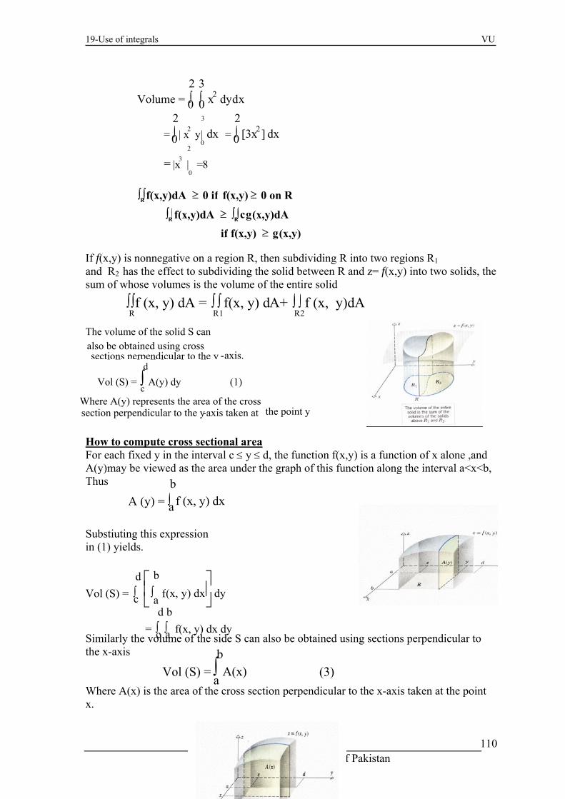
19-Use of integrals VU
© Copyright Virtual University of Pakistan 110
the effect to subdividing the solid between R and z= f(x,y) into two solids, the m of whose volumes is the volume of the entire solid
ow to compute cross sectional area
If f(x,y) is nonnegative on a region R, then subdividing R into two regions R1and R2 hassu H
or each fixed y in the interval c ≤ y ≤ d, the function f(x,y) is a function of x alone ,and
ilarly the volume of the side S can also be obtained using sections perpendicular to is
Where A(x) is the area of the cross section perpendicular to the x-axis taken at the point .
Volume = 0 0 x d ydx
=
∫2
∫3
2
∫2
0 | x2 y |
3
0d x = ∫
2
0 [3x2] dx
= | x3 |2
0= 8
∫ ∫ R f (x, y) dA = ∫ ∫
R 1 f(x, y) dA+ ∫ ∫
R2f (x, y)dA
FA(y)may be viewed as the area under the graph of this function along the interval a<x<b, Thus
Simthe x-ax
x
The volume of the solid S can
lso be obtained using cross a
sections perpendicular to the y - axis.
Vol (S) = ∫
d
c A(y) dy (1)
Where A(y) represents the area of the cross
section perpendicular to the y - axis taken at
the point y
A (y) = ∫b
a f (x, y) dx
Substiuting this expression ields.
ol (S) = ∫d
c ⎣ ⎢ ⎡
⎦ ⎥ ⎤
∫b
a
in (1) y
f (x , y ) dx dy
= ∫ d
c ∫b
a f(x, y) dx dy
∫ ∫
V
R f(x,y)dA ≥ 0 if f(x,y) ≥ 0 on R
∫ ∫R f(x,y)dA ≥ ∫ ∫R cg(x,y)dA
if f(x,y) ≥ g(x,y)
Vol (S) = ∫
b
a A(x) (3)

19-Use of integrals VU
For each fixed x in the interval a ≤ x ≤ b
e area A(x) is given by
oubl
the function f(x,y) is a function of alone, so that th D e integral for non-rectangular region Type I region is bounded the left and right by the vertical lines x=a and x=b and is ounded below and above by continuous curves y=g1(x) and y=g2(x) where g1(x) ≤ g2(x) for a≤ x ≤ b R is a type I region on which f(x, y) is continuous, then
y the me
A(x) = ∫
d
u bstituting this expression in
Vol (S) = ∫ b
a
f(x,y)dy
S(3) yields
⎣⎢⎡
⎦⎥⎤
∫ d
c f (x , y ) dy dx
= a ∫b∫d
c f(x,y) dy dx (4)
From eq (2) and eq (4) we have
∫ ∫ R
f (x,y) dA = ∫ d ∫bf(x,y) dx dy
c a
=∫ b
a ∫d
c f(x,y) dy dx
b If
∫ ∫Rf(x,y)dA = ∫
b g2(x)
a ∫g 1(x )
f(x,y)dydx (1) B
thod of cross section, the volume of S is also given by
© Copyright Virtual University of Pakistan
111

19-Use of integrals VU
where A at the fixed point x this cross section area
tends from g1(x) to g2(x) in the y-direction,
ype II region is bounded below and above by horizontal lines y=c and y=d and is ounded in the left and right by continuous curves x=h1(y) and x=h2(y) satisfying 1(y) ≤ h2(y) for for c≤ y ≤ d. f R is a type II region on which f (x, y) is continuous, then
olding x fixed and integrating with respect to y. function of x.
Vol (S) = (x) is the area of the cross section
∫ba A (x) dx (2)
so , A(x) = ∫g2(x)
g1(x)f(x, y) dy
Substituting this in ( 2) we obtainb g2(x)
ex Vol (S) = ∫a
∫g1(x)f(x, y) dy dx
Since the volume ofS is also given by ∫∫
Rf(x, y) dA = ∫
b
a ∫g2(x)
g1( x)f (x, y) dy dx Tbh. I Similarly, the partial definite integral with respect to f(x,y) is evaluated by hAn integral of the form produces a
∫ ∫R f(x,y)dA=∫
d
c ∫h 2 ( y )h 1 (y ) f(x,y)dx dy
d
c∫d
c f (x, y) dy
© Copyright Virtual University of Pakistan
112

20-Double integral for non-rectangular region VU
Lecture No -20 Double integral for non-rectangular region
ouble integral for non-rectangular region D
ype I region is bounded the left and right by vertical lines x=a and x=b and is bounded elow and above by curves y=g1(x) and y=g2(x) where g1(x) ≤ g2(x) for a≤ x≤ b
ontal lines y=c and y=d and is ng
1(y) ≤ h2(y) for c≤ y≤ d
rite double integral of the function f(x,y)on the region whose sketch is given
rite double integral of the function f(x,y)
∫ ∫
Tb Type II region is bounded below and above by the horiz
R f(x, y) dA = ∫
b
a ∫g2(x)
g1(x) f (x, y) dy dx
y = g2(x)
y = g 1(x)
a b
bounded on the left and right by the continuous curves x= h1(y) and x=h2(y) satisfyi
∫ ∫ R f(x,y) dxdy = ∫
d
c ∫h2(y)
h1(y) f(x,y)dx dy
h
x =h1(y)
c
d
x=h2(y)
W ∫
ln 8
1∫
ln y
0 f(x,y) dx
ln (ln 8)
∫ln8
e x f(x,y) y
∫ 0
W on the region whose sketch is given
© Copyright Virtual University of Pakistan
113

20-Double integral for non-rectangular region VU
∫
XA
E MPLE Draw the region and evaluate an equivalent integral with the order of integration reversed
he region of integration is given by the inequalities
XAMPLE
T
1
∫y2
f(x,y) dx dy
∫ ∫ √ x f (x, y) dy dx
∫
2
0 ∫
2x
x 2 (4x + 2) dy dx
x 2 ≤
0 0 1 1
0
y ≤
2x and 0 ≤ x ≤ 2.
∫ 4
0 ∫
√ y
y/2 (4x + 2) dx dy.
= ∫4
0 | 2x 2 + 2x|
√
y
y/2 dy
= ∫4
0 ⎣⎢⎢⎡
⎦⎥⎥⎤2y + 2
E The integral is over the region
y − y 2 − y dy
= ⎪ ⎪ ⎪ ⎪
⎪⎪⎪⎪y 2 +
4 3 y
3/2 − y 3
6 − y 2
2
4
0
= ⎣ ⎢ ⎢ ⎡
⎦⎥⎥⎤16 +
43 (4 )3/2 −
(4 )3
6 − 8
= 16 + 4 3 (8) −
64 6 − 8
= 8
valuate
I = ∫4
0∫
2
y y cos x
5 dx dy 0 < y < 4, x = y
nd x = 2
E
I = ∫2
0∫
x2
0 y cos x5 dy dx
a
x = 2
y = 4 (2,4)
O
x = 2
y = 4 (2,4)
x = 2
y = 4 (2,4)y = 4 (2,4)
y =x2
O
x = √y
© Copyright Virtual University of Pakistan
114

20-Double integral for non-rectangular region VU
Evaluate
he integral cannot be evaluated I the given order We which integration is performed
given by
= ∫
2
0 ⎣ ⎢ ⎢ ⎡
⎦ ⎥ ⎥ ⎤ y
2
2 cos x
5 x 2
0
dx
= ∫
2
0
4 x
2 cos x
5 dx
Tshall change the order of integration. The region Ris
= 1
10
= ⎣ ⎢ ⎢ ⎡
⎦ ⎥ ⎥ ⎤ 1
10
∫
2
0 cos x5 . (5x4) dx
sin x 5
2
0
= 1
10 sin 32
I = ∫
1/2
0 ∫
1
2x e y 2
dy dx
since e y2
has no antiderivative.
0 < x < 1
2 , y = 2x and y = 1
1/2
1 y = 2x Or x = y/2
O
This region is also enclosed by
x = 0, x = y
2 and 0 < y < 1
Thus
I = ∫
1
0 ∫
y/2
0 e dx dy
= ∫
1
0 y
2
y 2
e 2 dy
= ⎣ ⎢ ⎢ ⎡ 1
4
y
⎦ ⎥ ⎥ ⎤
e y 2
= 1
4
1
0
(e − 1)
31
y = lnx(3, ln3)
∫3
∫lnx
1 0 x dy dx
Reversing the order ofintegration
= ∫ln3
0∫
3
e y x dx dy
∫ln3
0 ⎪ ⎪ ⎪ ⎪ ⎪ ⎪ ⎪ ⎪ x2
2
3
e y dy =
12 ∫
ln3
0 [9 − e2y] dy=
© Copyright Virtual University of Pakistan
115

20-Double integral for non-rectangular region VU
Over view of Lecture # 20 Book Calsulus By Howard Anton
hapter # !7 Article # 17.2 age (858-863) Exercise set 17.2
21,22,23,25,27,35,37,38
1 2
⎪ ⎪ ⎪ ⎪ ⎪ ⎪ 9y − 2
⎪ ⎪ e2y
CP
=ln3
12
0
⎣ ⎢ ⎢ ⎡
⎦ ⎥ ⎥ ⎤ 9 ln3 − e 2ln3
2 + e 0
2
12
=
⎣ ⎢ ⎢ ⎡
⎦ ⎥ ⎥ ⎤ 9 ln3 − 92 +
1 2
12
=
[9 ln3 − 4 ]
92
=
ln3 − 2 =
© Copyright Virtual University of Pakistan
116

21-Examples VU
© Copyright Virtual University of Pakistan 117
Lecture No -21 Examples
Example
= − 1
8 ∫
4
0 e
- y 2 ( − 2y) dy
− 1
8 = | | e
- y 2 4
0
= −1
8 | | e
- 16 − c 0
=
1
8
⎝⎜⎜⎛
⎠
⎞1 − 1
e 16
4 (1,4)
y = 4x
y = 4
x = y/4
∫1
0∫
4
4xe - y
2 dy dx
Reversing the order ofintegration
∫4
0∫
y/4
0 e - y
2 dx dy
= ∫4
| | x e- y 2 y/4
0 dy = ∫
4
0 y4
e - y 2 dy
Calculate
∫∫R x sin x dA.
where R is the triangle in the xy- plane bounded by the x-axis ,the line y=x and the line x=1
We integrate first with respect to y and then with respect to x, we find
∫
1
0 ⎝ ⎜ ⎜ ⎜ ⎛
⎠
⎞
∫
x
0
sin x
x dy dx
1
= ∫ 0 ⎝
⎜ ⎜ ⎜ ⎛
⎠
⎞ sin x y x
y=x
] y=0 dx

21-Examples VU
1
0
sin= ∫ cos(0) 1 0.46x dx = − + ≈
= = − + ≈
EXAMPLE
1
0
sin cos(x dx∫ 0) 1 0.46
To evaualte this integral , we express is as an equivalent iterated integral with the order if integration reversed . For the inside integration, y is fixed and x varies from he line x = y/2 to the line x = 1. For the outside integration, y varies from 0 to 2, so the given iterated integral is equal to a double integral over the triangular region R. To reverse the order of integration, we treat R as a type I region, which enables us to write the given integral as
2
2 1xe d∫ ∫
02y
xdy
By changing the ord
By changing the order of integration we get, er of integration we get,
2
2 1xe dxdy
21 2x
xe d=0
2y
∫ ∫ ydx∫ ∫
EXAMPLE
0 0
Use a double integral to find the volume of the solid that is bounded above by the palne Z=4-x-y and below by the rectangle
= ∫10 [ex2
y]2x
y=0 dx
= ∫10 2xe x2
dx
= ex2 |1
0 = e − 1
∫ 2
0 ∫ 1
y/2 e x
Since there is no elementary
2 antiderivative of e
x2, the integral
∫ ∫1
ex2
dxdy
the x-integration first.
2 dxdy
y/20 cannot be evaluated by performing
R = {(x,y):0 < x < 1, 0 < y < 2}
© Copyright Virtual University of Pakistan
118

21-Examples VU
EXAMPLE Use a double integral to find the volume of the tetrahedron bounded by the coordinate planes and the plane z=4-4x y et-2 The t rahedron is bounded above by the plane.
--------------(1)
nes y + z = 4
z=4-4x-2y ----and below by the triangular region R
Find the volume of the solid bounded by the cylinder x2+y2 = 4 and the plaand z = 0.
The solid is bounded above by theplane z = 4 − y and below by theregion R within the circle x2 + y2 = 4. The volume is given by V = ∫ ∫
R (4 − y) dA
Treating R as a type I region we obtain
V = ∫ ∫R (4−4x−2y) dA
1 2-2x
= ∫10 (4−8x+4x2)dx
Thus, the volume is given by V = ∫ ∫
R (4 − 4x − 2y) dA
he region R is bounded by the x-axis, e y-axis, and the line y = 2 − 2x [set
= 0 in (1)], so that treating R as a ype I region yields.
V= ∫∫R (4−x−y) dA
= ∫2
0∫
1
0 (4−x−y) dx dy
= ∫2
0 ⎣⎢⎢⎡
⎦⎥⎥⎤4x −
x2
2 − xy1
x=0 dy
Tthzt
= ∫0 ∫ 0 (4 − 4x − 2y) dy dx
= ∫10 [4y−4xy−y2]
2-2xy=0
dx
= 34
© Copyright Virtual University of Pakistan
119
= ∫2
0 ⎝⎜⎜⎛
⎠⎟⎟⎞7
2 − y dy = ⎣⎢⎢⎡
⎦⎥⎥⎤7
2 y − y2
2
2
0
= 5
V = ∫
2
- 2
∫
√ 4 - x 2
- √ 4 - x 2 (4 − y) dy dx
= ∫
2
- 2 ⎣ ⎢ ⎢ ⎡
⎦ ⎥ ⎥ ⎤
4y − 1
2 y
2 √ 4 - x2
y= - √ 4-x 2 dx
= ∫
2
- 2 8 4 − x
2 dx

21-Examples VU
EXAMPLE Use double integral to find the volume of the solid that is bounded above by the paraboiled z=9x2 + y2 ,below by the plane z=0 and laterally by the planes
x = 0, y = 0, x = 3, y = 2
= ∫3
0 ⎝⎜⎜⎛
⎠⎟⎟⎞18x2 +
83
dx
= ⎪⎪⎪⎪
⎪⎪⎪⎪6x3 +
83 x
3
0
= 6 (27) + 8 = 170
olume = ∫3
0∫
2
0 (9x2 + y2) dy dx
= ∫3
0 ⎣⎢⎢⎡
⎦⎥⎥⎤
9x2y + y3
3
V
2
0 dx
= 8⎪⎪⎪⎪⎪
⎪⎪⎪⎪⎪
x 4-x2
2 + 42 sin-1
x2
2
-2
= 8| | 2sin-1(1) -2sin-1(-1)
= 8[2(π 2 ) + 2(
π 2 )]
=8(2π) = 16π
© Copyright Virtual University of Pakistan
120

22-Examples VU
© Copyright Virtual University of Pakistan 121
Lecture No -22 Examples
XAMPLE E
EXAMPLE
Use double integral to find the volume of the wedge cut from the cylinder 4x2+y2=9 by the plane z=0 and z=y+3
Solution:
Since we can write as94 22 =+ yx 2 2
2 193
2
x y+ =
⎛ ⎞⎜ ⎟⎝ ⎠
this is equation of
.
wer and upper limits for “x” are
ellipse
Now the Lo2 29 9y y− − −
2 2x and x= =
And upper and lower limits for “x” are 3− and respectively. So the required volume is
given by
32
2
93 2
3 92
( 3)
y
y
y dxd
−
− − −
+∫ ∫ y
∫ ∫ R xy dA
R is the region bounded by the Trapezium with the vertices
(1, 3) (5, 3) (2, 1) (4, 1)
S lope of AD = 3 − 1 1 − 2 = − 2
E quation of line AD x − 2)
x = − 2
A(2,1) B(4,1)
C(5,3)D(1,3)y − 1 = − 2 (y − 1 = − 2x + 4 − 2x = y − 5
y − 5
3 − 1
Slope of B C = 5 − 4 = 2
Equation of line BC y − 1 = 2 (x − 4) ⇒
y − 1 = 2x − 8 ⇒ 2x = y + 7 ⇒
x = 2
y + 7
∫ 3
1 ∫
( y+7 ) /2
- ( y - 5) /2 xy dx dy
= ∫3
1 (3y2 + 3y) dy = ∫
3
1y | x 2 |
( y+7 ) /2
- ( y - 5) /2 y dy
= ⎪ ⎪ ⎪ ⎪
⎪⎪⎪⎪y 3 +
3y 2 2
3 1
= (3)3 + 3 (3 )2
2 − 1 − 32 =38

22-Examples VU
( )
( )
[ ]
2
2
9329
3 2
3 2 2 2 2
2 2
332 22
33
3
9 9 9 93 3
9 3 9
1 2. 9 3 92 3
3 2
y
yxy x dy
y y y yy y dy
y y y dy
y y dy
−
−−−
−−
+
⎡ ⎤⎛ ⎞ ⎛ ⎞ ⎛ ⎞ ⎛ ⎞− − − −⎢ ⎥⎜ ⎟ ⎜ ⎟ ⎜ ⎟ ⎜ ⎟+ + +
=
3
3
2 2 2 2−⎜ ⎟ ⎜ ⎟ ⎜ ⎟ ⎜ ⎟⎢ ⎥⎝ ⎠ ⎝ ⎠ ⎝ ⎠ ⎝ ⎠
=
33 31
−
2 29 2 3 9y y dy y dy− − + −∫3 3
3
2 − −
⎣ ⎦
⎡ ⎤− + −⎣ ⎦
= −
− − + −
∫
∫
∫
∫
∫
=
=
321 . 0 3 9 3 9yy dy= − + − = −∫
32 19 27sin ( )yy π−+ =
3− 32 2 2−
XAMPLEE se double integral to find the volume of solid common to the cylinders x2+ y2=25 and
2+ z2=25
UALTED AS A DOUBLE INTEGRAL
Ux
Volume = 8 ∫5
0 ∫ 0
√25- x2
25 − x 2 dy dx
∫
5
0 = 8
AREA CALC
owever, the solid has congruent cross sections taken parallel to the xy-plan so that V = area of base x height=area of R.1 = area of R
ombining this with (1) yields the area formula
XAMPLE
H
25 − x2 | y | 25-x2
0 dx
= 8 ∫
5
0 (25 − x 2 ) dx
= 8 ⎪ ⎪ ⎪ ⎪
⎪ ⎪ ⎪ ⎪
25x − x 3
3
5
0
= 8 ⎝ ⎜ ⎜ ⎛
⎠
⎞ 125 − 125
3 = 8
⎝ ⎜ ⎜ ⎛
⎠
⎞ 250
3 =
2000
3 = 8
⎝ ⎜ ⎜ ⎜ ⎛
⎠ ⎞ 375 − 125
3
V = R 1 dA = ∫ ∫ ∫ ∫
RdA (1)
area of R =
C E
se a double integral to find the area of the region R enclosed between the parabola y = ½ x2 and the line y=2x
∫ ∫ RdA (2)
= ∫ 4
0∫
2x
x 2 /2 dy dx
U area of R= dA∫∫ R
© Copyright Virtual University of Pakistan
122

22-Examples VU
EXAMPLE
Find the area of the region R enclosed by the parabola y=x2 and the line y=x+2
= ∫ 4
0 [y ]2x
y=x2/2 dx = ∫
4
0 ⎝ ⎜ ⎜ ⎛ ⎠⎟⎟⎞2x −
12 x2 dx =
⎣⎢⎢⎡
⎦⎥⎥⎤x2 −
x3
6
4
0
= 163
Treating R as type II yields.
area of R=∫∫ R dA =∫
8
0 ∫
√ 2y
y/2 dx dy
8 √ 2x
= ∫ 0[ x]
y=x2 /2 dx
=⎣⎢⎢⎢⎡
⎦⎥⎥⎥⎤2
Exercise Set 17.2 (page 865): 21,22,23,25,27,35,37,38
23 y3/2 −
y2
4
8
0
=163 = ∫
0
8
⎝ ⎜ ⎜ ⎛
⎠⎟⎟⎞2y − 12 y dy
∫
2
- 1 ∫
y=x+2
y=x 2 dy dx
= ∫
2
- 1[y]x+ 2
x 2 dx
= ∫
2
- 1 [x + 2 − x2 ]dx
⎡ ⎤ x2
y = x+2
y = x2
= ⎣ ⎢ ⎢
⎦ ⎥ ⎥ 2 + 2x − 3
x3 2 9
- 1 = 2
© Copyright Virtual University of Pakistan
123

23-polar co-ordinate systems VU
Lecture No - 23 Polar Coordinate Systems
POLAR COORDIANTE SYSTEMS To form a polar coordinate system in a
P(r,θ
A THE POLAR COORDINATES OF POINT ARE NOT UNIQUE.
In general, if a point P has polar co-ordinate (r, θ ), then for any integer n=0,1,2,3,……. (r,θ +n.3600) and (r,θ +n.3600)
ces to a point, since r = 0. will agree that an arbitrary
ais the origin.
are also polar co-ordinates of p In the case where P is the origin, the line line segment OP reduBecause there is no clearly defined polar angle in this case, wePolar angle θ m y be used. Thus, for every θ may be used. Thus , for every θ ,the point (0, θ ) NEGATIVE VALUES OF R When we start graphing curves in polar coordinates, it will be desirable to allow negative alues for r. This will require a special definition. For motivation, consider the point P ith polar coordinates (3, 2250) We can reach this point by rotating the polar axis 2250
nd then moving forward from the origin 3 units along the terminal side of the angle. On e other hand, we can also reach the point P by rotating the polar axis 450 and then oving backward 3 units from the origin along the extension of the terminal side of the
or example, the polar coordinates, 315°), (1, − 45°), and (1, 675°) represent the same point
n polar coordinate systems.
)
O Origin Polar Axis
plane, we pick a fixed point O, called theorigin or pole, and using the origin as anendpoint we construct a ray, called the polar
nce from P to the originhe polar axis
axis. After selecting a unit of measurement,we may associate with any point P in theplane a pair of polar coordinates (r, θ), where r is the distaand θ measures the angle from tto the line segment OP. P(6,45 ) 0
P(3,2250)
(5,1200) The number r is called the radial distance of P and θ is called a polar angle of P. In the points (6, 45°), (3, 225°), (5, 120°), and (4, 330°) are plotted i
(4,3300)
1
1
vwathmangle
F(1all
(1,3150)
(1,6750)
(1,-450)
1
© Copyright Virtual University of Pakistan
124

23-polar co-ordinate systems VU
Sin is the xtension of the terminal side other angle
ce the terminal side of the angle 0180θ + e θ ,We shall define. (-r, θ ) and (r, With r=3 a
0180θ + ) to be polar coordinates for the same point . nd θ =45 in (2) if follows that (-3, 45 ) and (-3, 225 ) represent the sam
point. 0 0 0 e
AR COORDINATES RELATION BE EEN POLARTW AND ECTANGUL R
ION FORMULA FROM POLAR TO CARTESIAN COORDINATES
CONVERSAND VICE VERSA
Example Find the rectangular coordinates of the point P whose polar co-ordinates are (6,1350) Solution: Substituting the polar coordinates r = 6 and θ =1350 i x = cosn θ and y=sinθ yeilds Thus, the rectangular coordinates of the point P are (
ight also be denoted by ( − 3, 45 °), ith the minus sign serving todicate that the point is on the
xtension of the angle’s terminal sidether than on the terminal side itself.
This suggests that the point (3, 225 °)
P(3,2250) Polar Axis
Terminal Sides
P(-3,2250) Polar Axis
mwinera
o x= rcos θ
r
θx
y P(x,y)P(r,θ)
y = r sinθ
o xyr
P(x, y) =P(r, θ)
θ
x = r cos θ
y = r si θn
x2 + y2
y/ x =tanθ
= r2x
x = 6 cos 135 ° = 6 (− 2 /2) = − 3 2 y = 6 sin 135 ° = 6 ( 2 /2) = 3 2
− 3 2 , 3 2 )
P
r = 6 135°
© Copyright Virtual University of Pakistan
125

23-polar co-ordinate systems VU
Example: Find polar coordinates of the point P whose rectangular coordinates are ( 2,2 3)− Solution: We will find polar coordinates (r, θ ) of P such that r >0 and 0 2θ π≤ ≤ .
2 2 2 2( 2) (2 3) 4 12 16 4r x y= + = − + = + = =
12 3 2tan 3 tan ( 3)2 3
yx
πθ θ −= = = − ⇒ = − =−
From this we have (-2,2 3 ) lies in the second quadrant of r co-ordinates of P have the form
P. All other Pola
2 5(4, 2 ) ( 4, 2 ) , int3 3
n or n Where n is egerπ ππ π+ − +
LINES IN POLAR COORDIANTES A line perpendicular to the x-axis and passing through the poiwith (a,0) has the equation x=a . To express t olar co-ordinates we
nt with xy co-ordinates his equation in p
substitute x = r cos θ ⇒ a = rcos θ --------(1)
By substitution x = rcosθ and y = rsinθ in the equation Ax +By +C = 0 . We obtain the general polar form of the line,
For Any constant θ0, the equationθ = θ0 (3) is satisfied by the coordinates of all points of the form P (r, θ ),
the line through igin making an angle of θ0
adians) with the polar axis.
line parallel to the x-axis that eets the y-axis it the point with
y-coordinates (0, b) has the
r sin θ = b (2) as the polar equation of this line. This makes sense geometrically since each point P (r, θ) on this line will yield the value b for r sin θ
eometrically since each oint P (r, θ) on this line will ield the value a for r cos θ.
This result makes sense
0regardless of the value of r. Thus, the equation represents the or(r
Amxequation y = b.
ubstituting y = r sin θ yields.
r (A cosθ + B sinθ) + C = 0
gpy
S
© Copyright Virtual University of Pakistan
126

23-polar co-ordinate systems VU
CIRCLES IN POLAR COORDINATES
SOME SPECIAL CASES OF EQUATION OF CIRCLE IN POLAR COORDINATES
Lecture No -24 Sketching
If a circle of radius a han the x-axis and passes
e center is to origin
his equation makes sense eometrically since the circle f radius a, centered at the rigin, consists of all points (r, θ) for which r = a, gardless of the value of θ
hose center has polar coordinates 0, θ0). If we let P(r, θ) be an rbitrary point on the circle, and if
we apply the law of cosines to the triangle OCP we obtain r2 − 2rr0 cos (θ − θ0) + r2
0 = a2 (1)
Let us try to find the polar equation of a circle whose radius is a and w(ra
A circle of radius a, centered at the rigin, has an especially simple pola
s its center through the o
origin, then the polar coordinates of the center are either (a, 0) or (a, π) depending on whether th
the the right or left of
TgooPre
o r quation. If we let r 0 = 0 in (1), we btain r2 = a2 or, since a > 0, r = a
eo
© Copyright Virtual University of Pakistan
127
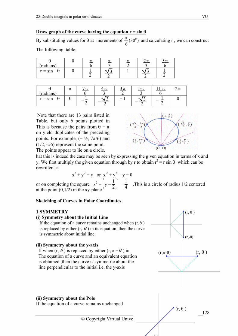
25-Double intagrals in polar co-ordinates VU
Draw graph of the curve having the equation r = sin θ 0(30 )
6πBy substituting values for θ at increments of and calculating r , we can construct
The following table:
t this is indeed the case may be seen by expressing the given equation in terms of x and ation through by r to obtain r2 = r sin θ which can be
.This is a circle of radius 1\2 centered t the point (0,1/2) in the xy-plane.
ketching of Curves in Polar Coordinates
hay. We first multiply the given equrewritten as or on completing the square a S
hen (r,
1.SYMMETRY (i) Symmetry about the Initial Line
ed If the equation of a curve remains unchang w θ ) is replaced by either (r,-θ ) in its equation ,then the curve
etry about the y-axis If when (r,
is symmetric about initial line. ii) Symm(
θ ) is replaced by either (r,π θ− ) in The equation of a curve and an equivalent equat n
line perpendicular to the initial i.e, the y-axis
ii) Symmetry about the Pole If the equation of a curve remains unchanged
e pairs from θ = π
acle.
θ (radians)
0 π 6
π3 π
2 2 π3 5 π
6 r = sin θ 0 1
2 3
2 1 32
12
θ
(radians) π 7 π
6 4 π3 3 π
2 5 π3 11 π
6 2 π
io is obtained ,then the curve is symmetric about the
(
Note that there are 13 pairs listed in able, but only 6 points plotted in T
This is because thon yield duplicates of the precedingpoints. For example, (− ½, 7π/6) and (1/2, π/6) represent the s me point. The points appear to lie on a cir
r = sin θ 0 − 1 2 − 3
2 1 −− 3
2 − 12 0
x + y = y or x + y 2 2 2 2 − y = 0 2
x 2 + ⎝⎜⎜⎛
⎠⎞
y − 12 =
14
© Copyright Virtual University of Pakistan
128
(r, θ )
(r,-θ)
(r, θ )(r,π-θ)
(r, θ )
( θ )

25-Double intagrals in polar co-ordinates VU
when either (-r, θ ) or is substituted for (r, θ ) in its equation ,then the curve is symmetric bout the pole. In such a case ,the center of a
the curve.
2. Position Of The Pole Relative To The Curve See whether the pole on the curve by putting r=0for
in the equation of the curve and solving θ .
3. Table Of Values Construct a sufficiently complete table of valuesthe graph of a curve. II Position Of The Pole Relative To The Curve.
. This can be of great help in sketching
When r = 0 , θ = 0 .Hence the curve passes through the pole.
n re ve in s, we obtain the curve.
CARDIDOIDS AND LIMACONS
O flecting the cur about the x-axi
III. Table of Values θ 0 π/3 π/2 2π/3 π
r=a (1−cosθ) 0 a/2 a 3a/2 2a As θ varies from 0 to π, cos θ decreases steadily from 1 to − 1, and 1 − cos θ
creases steadily from 0 to 2. Thus, as θ ries from 0 to π, the value of
r = a (1 − cos θ) will increase steadily from an initial value of r = 0 to a final value of r = 2a.
inva
CARDIOIDS
r = a (1 – cos θ) r = a (1 + cos θ)
r = a (1 + sin θ)r = a (1 – sin θ)
θ = π θ =0, r=0r = 2a
θ = π
r = 0O O A
C (2a, - π/2)
O
O
(0 , π/2) D
π/2)(0, -
© Copyright Virtual University of Pakistan
129

25-Double intagrals in polar co-ordinates VU
r=a+b sin θ, r = a−bsin θ
=a+b cos θ, r = a−bcos θ The equations of above form produce polar curves called limacons. Because of the heart-
con relative to the polar axis depends on whether sin θ or cos θ appears in the equation and whether the + or − occurs.
r
shaped appearance of the curve in the case a = b, limacons of this type are called cardioids. The position of the lima
LEMINSCATE If a > 0, then equation of the form r2 = a2 cos2θ, r2 = − a2 cos 2θ r2 = a2 sin 2θ, r2 = − a2 sin 2θ represent propeller-shaped curves, called lemiscates (from the Greek word “lemnicos” for a looped ribbon resembling the Fig 8. The lemniscates are centered at the origin, but the
ition relative to the polar axis depends on the sign preceding the a2 and whether sin 2θ or cos 2θ appears in the equation.
Examp
pos
le
© Copyright Virtual University of Pakistan
130

25-Double intagrals in polar co-ordinates VU
r2 = 4 cos 2 θ The equation represents a lemniscate. The graph is symmetric about the
xis. Therefore, we can obtain each graph by first sketching the portion f the graph in the range 0 <
x-axis and the y-ao θ < π/2 and then reflecting
the x- and y-axes.The curve passes n θ = π/4, so the line θ = π/4 is
t θ varies from 0 to π/4,
range π/4 < θ < π/2, the quantity cos2θ is negative, so there are no real values of r satisfying first equation. Thus, there are no points on the graph for such θ. The entire graph is obtained by reflecting the curve about the x-axis and then reflecting the resulting curve about the y-axis. ROSE CURVES
that portion about through the origin whetangent to the curve a the origin.As the value of cos2θ decreases steadily from 1 to 0, so that rdecreases steadily from 2 to 0.For θ in the
Equations of the form r = a sin nθ and r = a cos n θ
if n is even
The
r sinθ or cosθ appears in the equation.
represent flower-shaped curves called roses. The rose has n equally spaced petals or loops if n is odd and 2n equally spaced petals
orientation of the rose relative to the polar axis depends on the sign of the constant a and whethe SPIRAL A curve that “winds around the origin” infinitely many times in such a way that r
eadily as θ increases is called a spiral. The most common des, which has an equation of the form.
(θ >
increases (or decreases) stexample is the spiral of Archime
0) or r = aθ (θ < 0) r = aθ In these equations, θ is in radians and a is positive. EXAMPLE Sketch the curve r = θ (θ > 0) in polar coordinates.
a = 1; thus, it represents an Archimedean spiral. origin is on the curve and the polar axis is tangent to the
es and noting that r increases steadily as θ increases. The intersections ith the x-axis occur when
θ = 0, π, 2π, 3π, …….
This is an equation of spiral withSince r = 0 when θ = 0, thespiral. A reasonably accurate sketch may be obtained by plotting the intersections of the spiral with the x and y axw
© Copyright Virtual University of Pakistan
131

25-Double intagrals in polar co-ordinates VU
at which points r has the values r = 0, π, 2π, 3π,….. and the intersections with the y-axis occur when
θ = π2 ,
3π2 ,
5π2 ,
7π2 , ……
at which points r has the values
r = π2 ,
3π2 ,
5π2 ,
7π2 , ……
m the origin, the Archimedean spirals r = θ (θ >Starting fro 0) loops counterclockwise round the origin.
a
© Copyright Virtual University of Pakistan
132

25-Double intagrals in polar co-ordinates VU
Lecture No -25 Double integrals in polar co-ordinates Double integrals in which the integrand and the region of integration are expressed in polar coordinates are important for two reasons: First, they arise naturally in many applications, and second, many double integrals in rectangular coordinates are more easily evaluated if they are converted to polar coordinates. The function z = f(r,θ) to be integrated over the region R As shown in the Fig.
© Copyright Virtual University of Pakistan
133
INTEGRALS IN POLAR COORDIATES When we defined the double integral of a function over a region R in the xy-plane, we began by cutting R into rectangles whose sides were parallel to the coordinate axes. These were the natural shapes to use because their sides have either constant x-values or constant y-values. In polar coordintes, the natural shape is a “polar rectangle” whose sides have constant r and θ- values. Suppose that a function f (r, θ) is defined over a region R that is bounded by the ray θ = α and θ = β and by the continuous curves r = r1 (θ) and r = r2(θ). Suppose also that 0 < r1(θ) < r2(θ) < a for every value of θ between α and β. Then R lies in a fan-shaped region Q defined by the inequalities 0 < r < a and α < θ < β. Then the double integral in polar coordinates is given as
∫ ∫ R 1 ( )r r
f (r,θ) dA = ( )
( , )r r2
f r drdθθ β
θ α θ
θ θ=
∫ ∫ =
= =
How to find limits of integration from sketch Step 1. Since θ is held fixed for the first integration, draw a radial line from the origin through the region R at a fixed angle θ. This line crosses the boundary of R at most twice. The innermost point of intersection is one the curve r = r1(θ) and the outermost point is on the curve r = r2(θ). These intersections determine the r-limits of integration. Step 2. Imagine rotating a ray along the positive x-axis one revolution counterclockwise about the origin. The smallest angle at which this ray intersects the region R is θ = α and
le is θ = β. This yields the θ-limits of the integration. the largest angEXAMPLE Find the limits of integration for integrating f (r, θ) over the region R that lies inside the
1 + cos θ and outside the circle r = 1.
We sketch the region and label the bounding urves.
rom
cardioid r =Solution: Step 1. c Step 2. The r-limits of integration. A typical ray f

25-Double intagrals in polar co-ordinates VU
The origin enters R where r =1 and leaves where
the
origin that interse from θ = −
r =1+cos θ. Step 3. The θ-limits of integration. The rays from
π2 to θ = 2
πct R run .
The i s ∫
/2
-π/2∫
θ
1 f (r, θ) r dr dθ
θ
θ) rdr dθ
π 1+cos
ntegral iπ/2 1+cos
= 2 ∫0
∫1
f(r,
EXAMPLE ∫ sin Evalaute ∫R
θ dA
Where R is the region ion the first quadrant that is outside the circle r = 2 and inside the 2(1+cosθ).
Solution:
∫ ∫R sin θ dA=∫
/2
0∫
2(1+cosθ
(sin θ) r dr dθ
= ∫
cardioid r =
π )
2
π/21
0 2 r2 sin θ]
cosθ
r=2 dθ
= 2∫
/2
[(1+cosθ)2sin θ−sinθ]
= 2 ⎢ ⎦⎥−
2(1+ )
π
0dθ
⎡ ⎤1⎣ 3 (1 + cosθ)3 + cosθ
/2
0
= ⎣⎢ ⎦⎥− 3
π
⎡ ⎤1 − ⎝⎜ ⎠⎟− 3
⎛ ⎞5 = 3
8
EXAMPLE Use a double polar integral to find the area enclosed by the three-petaled rose r = sin 3θ.
te the area of the petal R in the first quadrant and multiply by three. Solution:
A = 3 dA = 3 ∫0
∫0
sin3θ
r dr dθ = ∫0 2
We calcula
∫ ∫
π/3 π/3r2
R |
i θ
0 dr dθ
= 2
s n3
3 ∫
/3
0 sin2 3θ dθ = 4
π
3 ∫
/3
0 (1−cos 6θ) dθ
= 4
π
3 ⎣⎢ ⎦⎥θ −
sin 6θ6
⎡ ⎤π
⎡ ⎤3/3
0 = ⎣⎢ ⎦⎥4 θ − 24
3 sin 6θ
/3
0
= 4
π1 π
EXAMPLE
© Copyright Virtual University of Pakistan
134

25-Double intagrals in polar co-ordinates VU
Find the area enclosed by the lemniscate r2 = 4 cos2θ. The total area is four times the first-quadrant portion.
Solution:
A = 4 ∫
π/4
0∫0
√4 cos2θ
r dr dθ=A ∫
π/4
0
4 2
0
22
r cos
r
r θ√=
=
⎡ ⎤⎢ ⎥⎣ ⎦
dθ
= 4 ∫
π/4
02cos 2θ dθ = 4 sin 2θ]
π/4
0 = 4.
CHANGING CARTESIAN INTEGRALS INTO POLAR INTEGRALS The procedure for changing a Cartesian integral ∫ ∫
Rf(x, y) dx dy into a polar integral has
two steps. Step 1. Substiute x = r cos θ and y = r sinθ, and replace dx dy by r dr dθ in the Cartesian integral. Step 2. Supply polar limits of integration for the boundary of R. The Cartesian integral then becomes ∫ ∫R f(x,y) dx dy=∫ ∫
G f(rcosθ, rsinθ)r dr dθ
where G denotes the region of integration in polar coordinates. Notice that dx dy is not replaced by dr dθ but by r dr dθ. EXAMPLE
Evalaute the double integral ∫
1
0∫
√1-x2
0(x2 + y2) dy dx by changing to polar coordinates.
The region of integration is bounded by
0 < y < 1 − x2 and 0 < x < 1
y = 1 − x2 is the circle x2 + y2 = 1, r = 1 On changing into the polar coordinates, the given integral is
∫
π/2
0∫
1
0 r3 dr dθ = ∫
π/2
0 ⎪⎪⎪
⎪⎪⎪r4
4
1
0 dθ = ∫
π/2
0
14 dθ = ⎪⎪
⎪⎪⎪⎪θ
4
π/2
0 =
π8
EXAMPLE
Evaluate I = ∫D∫
dx dyx2 + y2 by changing to polar coordinates,
where D is the region in the first quadrant between the circles. 0x2+y2=a2 and x2+y2=b2, 0<a<b
I = ∫
π/2
0∫
b
a r dr dθ
r2 = ∫
π/2
0 [ln r]
b
a dθ
© Copyright Virtual University of Pakistan
135

25-Double intagrals in polar co-ordinates VU
= ∫
π/2
0 ln ⎝⎜
⎛⎠⎟⎞b
a dθ= ⎣⎢⎡
⎦⎥⎤θ ln ⎝⎜
⎛⎠⎟⎞b
a
π/2
0
= π2 ln ⎝⎜
⎛⎠⎟⎞b
a .
EXAMPLE 21 x1
Evaluate the double integral 2 2( )0 0
x y dy dx+∫ ∫−
by changing to polar coordinates.
21 x− and The region of integration is bounded by 0 < y < 0 ≤ x ≤ 1
= 21 x− is the circle 2 2x y+y =1, r = 1 n e polar coordinates, the given integral is O changing into th
1/ 2 1 / 2 / 24
/ 230
0 0 0 00
1 1 1 ( / 2) / 84 4 4 4rr drd d d
π π ππθ θ θ θ π π= = = = =∫ ∫ ∫ ∫
© Copyright Virtual University of Pakistan
136
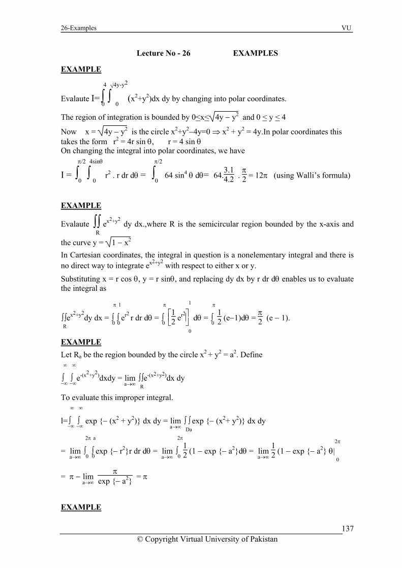
26-Examples VU
Lecture No - 26 EXAMPLES
EXAMPLE
Evalaute I=∫0∫
0(x
4 √4y-y2
2+y2)dx dy by changing into polar coordinates.
The region of integration is bounded by 0<x< 4y − y2 and 0 < y < 4
Now x = 4y − y2 is the circle x2+y2−4y=0 ⇒ x2 2 olar coordinates this th for
On changing the integral into olar coordinates, w vπ/2
0
4sinθ
2 . r dr dθ = ∫π/2
0 64 sin4 θ dθ= 64.
3.14.2
+ y = 4y.In ptakes e m r2 = 4r sin θ, r = 4 sin θ
p e ha e
. π2 = 12π (using Walli’s formula) I = ∫ ∫ r
0
EXAMPLE
Evalaute ∫∫R ex2+y2 dy dx.,where R is the semicircular region bounded by the x-axis and
the curve y = 1 − x2 In Cartesian coordinates, the integral in question is a nonelementary integral and there is no direct way to integrate ex2+y2 with respect to either x or y.
θ i θinte
π 1
r2 π
⎡ ⎤1
Substituting x = r cos , y = r s nθ, and replacing dy dx by r dr d enables us to evaluate the gral as
∫ ∫Re dy dx = ∫
0∫0e r dr dθ = ∫
0 ⎣⎢ ⎦⎥2
x2+y2 e dθ = ∫
0 2
r2
0
π
11
(e−1)dθ = 2π
(e − 1).
EXAMPLE Let Ra be the region bounded by the circle x2 + y2 = a2. Define
∫−∞
e2+y2)dxdy = lim ∫ ∫e-(x2+y2)dx dy
To evaluate this improper integra∞ ∞
lima→∞ 0 0
= lima→∞
∫
2π
0
12
∞ ∞
−∞ ∫ -(x
a→∞ R
l.
l=∫−∞
∫−∞
exp {− (x2 + y2)} dx dy = lima→∞
∫ ∫Da
exp {− (x2+ y2)} dx dy
= ∫
2π
∫
a
exp {− r2}r dr dθ (1 − exp {− a2}dθ = lima→∞
12 (1 − exp {− a2} θ|
2π
0
a→∞
π− a2}= π − lim exp { = π
EXAMPLE
© Copyright Virtual University of Pakistan
137

26-Examples VU
Prove that ∫0
e
∞
-t2 dt=12 π.
l = ∫
∞
-∞∫
∞ ∞ ∞ ∞ ∞
−x2} dx] ∞ ∞ a 2 a
a
2→∞
a a
2)}dx dy4lima→∞
[∫
∞
0exp{-t2}dt]
2
= π
∞
0t]
2
= π/4 ⇒ ∫
∞
0exp {− t2} dt =
-∞exp{−(x2+y2)} dx dy=∫
-∞exp{−y2}[∫
-∞exp{−x2}dx] dy = [∫
-∞exp{−y2}dy][ ∫
-∞exp{
= [∫-∞
exp{−t2}dt][ ∫-∞
exp{−t2} dt] =lima→∞
[∫-a exp {− t2} dt] = 4lim
a→∞ [∫
0 exp {− t2} dt]
2
Hence we have 4lima→∞
[∫0 exp{− t } dt ]= lim
a∫-a∫-aexp{−(x2+y
π2 l
a→∞im [∫ exp{-t2}d
THEOREM Let G be the rectangular box defined by the inequalities a < x < b, c < y < d, k < z <
If f is continuous on the region G, then ∫∫∫ f(x, y, z) dV = ∫b
∫d
G ∫ f (x, y, z) dz dy dx
er
∫b
a ∫
d
c ∫
k f (x, y, z) dx dy dz
b d
, y, z) dx dz dy= ∫k
∫b
a ∫
d
c f (x, y, z) dz dx dy
EXAMPLE
a c k
Moreover, the iterated integral on the right can be replaced with any of the five othiterated integrals that result by altering the order of integration.
= ∫d
c ∫
k ∫
b
a f (x, y, z) dy dz dx = ∫
d
c ∫
b
a ∫
k f (x, y, z) dy dx dz=
= ∫a
∫k
∫c
f (x
valaute the triple integral ∫ ∫ ∫ 12xy2z3 dV over the rectangular box G defined by the E
G
inequalities − 1 < x < 2, 0 < y < 3, 0 < z < 2. We first integrate with re olding x and y fixed, then with respect to y holding x
2
-1
3 3
0
4]2
z=0 dy dx = ∫
2
-1 ∫
3
0 48xy2 dy dx
∫
2
-1[16xy3]
3
y=0dx=∫
2
-1 432x dx = 216x2 ]
2
-1 = 648
spect to z, hfixed, and finally with respect to x.
∫ ∫ ∫12xy2z3 dV= ∫ ∫0 ∫
2
0 12xy2z3dzdydx = ∫
2
-1 ∫ [3xy2z
G
=
© Copyright Virtual University of Pakistan
138

26-Examples VU
EXAMPLE
Evala teu ∫∫R∫ (x − 2y + z) dx dy dz Region R : 0 < x , 1, 0 < y < x2, 0 < z < x + y
=0∫
y
z) ∫ ∫ ⎪ ⎪⎪(x + z)2
2 ∫0∫
0(x − 2y + dz dy dx=
0 0 ⎪⎪ ⎪
− 2y1 x2 x+ 1 x2
x+y
01 x2
dy dx
= ⎡(x−2y+x+y)2
∫0∫
0 ⎣⎢ ⎦⎥⎤
2 − −2
(x 2y)2
dy dx = 21 ∫ (3x2 − 3y2) dy dx=
32
1 x2
∫0
⎪⎪⎪
⎪⎪⎪x2y −
y3
13
x2
0∫
0 0 dx
3=2
0 ⎝⎜x4 − ∫ ⎛⎠⎟⎞x
z
16
dx = 32 ⎪⎪
⎪⎪⎪⎪x
55
− x21
7 1
0 =
32 ⎣⎢
⎡⎦⎥⎤1
5 − 121 =
835
Example:
Evalaute ∫∫S∫ xyzd x dy dz Where S = {(x,y,z):x2+y2+z2<1, x > 0, y > 0, z > 0}
S is the sphere x2 + y2 + z2 = 1 .Since x, y, z are al +ve so we have to consider only the +ve octant of the sphere. Now x2 + y2 + z2 = 1 . So that z = 1 − x2 − y2 The Projection of the sphere on xy plan is the circle x2 2 = 1. + yThis circle is covered as y-varies from 0 to 1 − x2 and x varies from 0 to 1.
1 √1- √ -x2 1 √1-5
∫∫x2
∫1 -y2
y dx = ∫ ∫x2
xy ⎪⎪ ⎪⎪z √
R∫ xyz dx dy dz= ∫
0∫
0 0 xyz dz d
0 0 ⎪ ⎪20
1 √1-2
1-x2-y2
dy dx
x2
1 − y2
= ∫0∫
0xy ⎝⎜
⎛⎠⎟⎞− x
2 dy dx = 21 ∫
0∫
0x (y − x y − y ) dy dx
1 √1-x2
2 3
= 12 ∫
0 ⎝ ⎠2
12
x ⎜⎛ ⎟⎞y
−x y2
22
4− y4
2
|0
dx= 14 ∫ ⎦
⎥− ( x(1−x2)
21⎡ ⎤√1-x
0x ⎣
⎢1 x2−x2 1− 2)− 2 dx
18= ∫
0(x − 2x3 + x5) dx=
18
1
⎪⎪⎪
⎪⎪⎪x
22
− x2
4
+ x6
6 1
0 =
18 ⎝⎜
⎛⎠⎟⎞1
2 − 12 +
16 =
148
© Copyright Virtual University of Pakistan
139
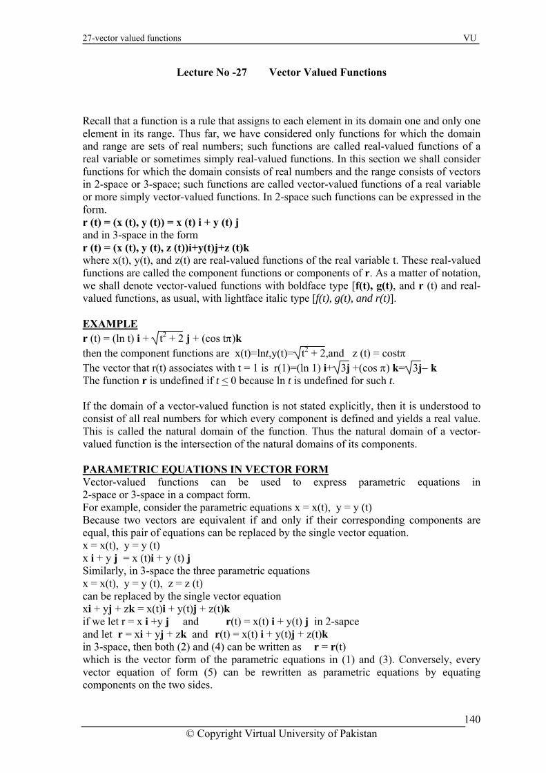
27-vector valued functions VU
Lecture No -27 Vector Valued Functions
mply vector-valued functions. In 2-space such functions can be expressed in the
+ y (t) j
nd r (t) and real-alued functions, as usual, with lightface italic type [f(t), g(t), and r(t)].
Recall that a function is a rule that assigns to each element in its domain one and only one element in its range. Thus far, we have considered only functions for which the domain and range are sets of real numbers; such functions are called real-valued functions of a real variable or sometimes simply real-valued functions. In this section we shall consider functions for which the domain consists of real numbers and the range consists of vectors in 2-space or 3-space; such functions are called vector-valued functions of a real variable or more siform. r (t) = (x (t), y (t)) = x (t) i and in 3-space in the form r (t) = (x (t), y (t), z (t))i+y(t)j+z (t)k where x(t), y(t), and z(t) are real-valued functions of the real variable t. These real-valued functions are called the component functions or components of r. As a matter of notation, we shall denote vector-valued functions with boldface type [f(t), g(t), av EXAMPLE r (t) = (ln t) i + t2 + 2 j + (cos tπ)k then the component functions are x(t)=lnt,y(t)= t2 + 2,and z (t) = costπ The vector that r(t) associates with t = 1 is r(1)=(ln 1) i+ 3j +(cos π) k= 3j− k
he function r is undefined if t <T 0 because ln t is undefined for such t.
of a vector-alued function is the intersection of the natural domains of its components.
If the domain of a vector-valued function is not stated explicitly, then it is understood to consist of all real numbers for which every component is defined and yields a real value. This is called the natural domain of the function. Thus the natural domainv PARAMETRIC EQUATIONS IN VECTOR FORM Vector-valued functions can be used to express parametric equations in
omponents are quations can be replaced by the single vector equation.
e parametric equations
r equation
sapce
can be rewritten as parametric equations by equating omponents on the two sides.
2-space or 3-space in a compact form. For example, consider the parametric equations x = x(t), y = y (t) Because two vectors are equivalent if and only if their corresponding cequal, this pair of ex = x(t), y = y (t) x i + y j = x (t)i + y (t) j Similarly, in 3-space the threx = x(t), y = y (t), z = z (t) can be replaced by the single vectoxi + yj + zk = x(t)i + y(t)j + z(t)k if we let r = x i +y j and r(t) = x(t) i + y(t) j in 2-and let r = xi + yj + zk and r(t) = x(t) i + y(t)j + z(t)k in 3-space, then both (2) and (4) can be written as r = r(t) which is the vector form of the parametric equations in (1) and (3). Conversely, every vector equation of form (5)c
© Copyright Virtual University of Pakistan
140

27-vector valued functions VU
EXAMPLE Express the given ra pa metric equations as a single vector equation.
(a) Usi ations as components of a vector yields.
(b) Proxi + yj + zk = (cos t)i + (sin t)j + tk
(a) x = t2, y = 3t (b) x = cost, y = sint, z = t
ng the two sides of the equx i + y j = t2 i + 3t j ceeding as in part (a) yields
EXAMPLE Find parametric equations that correspond to the vector equation
re ponents yields. = t3 + 1, y = 3, z = et
x i + y j + z k = (t3 + l) i + 3 j + et k Equating cor sponding comx GRAPHS OF VECOR-VALUED FUNCTOINS One method for interpreting a vector-valued function r(t) in 2-space or 3-space geometrically is to position the vector
d by the tip of the vector r
set of parametric equations, so C is also called the raph of these parametric equations.
r = r (t) with its initial point at the origin, and let C be the curve generate as the parameter t varies The vector r, when positioned in this way, is called the radius vector or position vector of C, and C is called the graph of the function r (t) or, equivalently, the graph of the equation r = r (t). The vector equation r = r (t) is equivalent to a g EXAMPLE Sketch the graph of the vector-valued function r(t) = (cos t)i + (sin t)j, 0 < t < 2π
ector equation The graph of r (t) is the graph of the vxi+yj = (cos t)i + (sin t)j, 0 < t < 2π or equivalently, it is the graph of the parametric equations x = cos t, y = sin t (0 < t < 2π) This is a circle of radius 1 that is centered at the origin with the direction of increasing t ounterclockwise. The graph and a radius vector are shown in Fig. c
© Copyright Virtual University of Pakistan
141

27-vector valued functions VU
EXAMPLE Sketch the graph of the vector-valued function r(t) = (cos t)i+(sin t)j+2k, 0 < t < 2π
ctor equation The graph of r(t) is the graph of the vexi+yj+zk=(cost)i+(sint)j+2k, 0<t<2π or, equivalently, it is the graph o the parametric equations x=cos t, y = sin t, z=2 (0 < t < 2π) From the last equation, the tip o the radius vecor traces a curve in the plane z = 2, and from the first two equations and the preceding example, the curve is a circle of radius 1 centered on the z-axis and traced counterclockwise looking down the z-axis. The graph nd a radius vector are shown in Fig. a
EXAMPLE Sketch the graph of the vector-valued function r(t) = (a cos t)i + (a sin t)j + (ct)k
he parametric equations.
tly
curve that wraps around a red on the z-axis.
his curve is called a circular helix.
where a and c are positive constant. The graph of r(t) is the graph of tx = a cos t, y = a sin t, z = ct As the parameter t increases, the value of z = ct also increases, so the point (x, y, z) moves upward. However, as t increases, the point (x, y, z) also moves in a path direcover the circle. x = a cos t, y = a sin t in the xy-plane. The combination of these upward and circular motions produces a corkscrew-shapedright-circular cylinder of radius a centeT EXAMPLE Describe the graph of the vector equation r = (− 2 + t)i + 3tj + (5 − 4t)k The corresponding parametric equations are x = − 2 + t, y = 3t, z = 5 − 4t The graph is the line in 3-space that passes through the point (− 2, 0, 5) and is parallel to
e vector i + 3j − 4k. th EXAMPLE The graph of the vector-valued function r (t) = t i + t2 j + t3 k is called a twisted cubic. Show that this curve lies o the parabolic cylinder y = x2, and sketch the graph for t > 0
© Copyright Virtual University of Pakistan
142

27-vector valued functions VU
The corresponding parametric equations are x = t, y = t2, z = t3
Eliminating the parameter t in the equations for x and y yields y = x2, so the curve lies on the parabolic cylinder with this equation. The curve starts at the origin for t = 0; as t increases, so do x, y, and z, so the curve is traced in the upward direction, moving away
om the origin along the cylinder. fr GRAPHS OF CONSTANT VECOR-VALUED FUNCTIONS If c is a constant vector in the sense that it does not depend on a parameter, then the graph
r (x0, y0), and if
= x0i + y0j + z0k (in 3-space), then the graph is the point (x0, y0, z0).
of = c is a single point since the radius vector remains fixed with its tip at c. If c = x0i + y0j (in 2-space), then the graph is the pointc EXAMPLE The graph of the equation r = 2i + 3j − k is the point (2, 3, − 1) in 3-space. If r(t) is a vector-valued function, then for each value of the parameter t, the expression
alued function of t because the norm (or length of r(t) is a real number.
hen ||r(t)|| =
||r(t)|| is a real-v For example, If r(t) = t i + (t − 1) j
t2 + (t − 1)2 which is a real-valued function of t. T EXAMPLE The graph of r (t) = (cos t)i + (sin t)j + 2k, 0<t<2π is a circle of radius 1 centered on th z-axis and lying in the plane ze = 2. This circle lies on the surface of a sphere of radius 5 bec ause for each value of t ||r(t)|| = cos2t + sin2t + t = 1 + 4 = 5 which shows that each point on the circle is a distance of 5 units from the origin.
© Copyright Virtual University of Pakistan
143

28-Limits of vector valued functions VU
Lecture No -28 Limits of Vector Valued Functions
he r a function r(t) = x (t)i + y (t)j in 2-space we define.
= x(t)i + y(t)j + z(t)k
limits t→α+ ,
t→α− limt→+∞
, and t→−∞
. It follows from (1) and (2) that
ng that the length and direction of r (t) pproach the length and direction of L as t → α
The limit of a vector-valued functions is defined to be the vector that results by taking tlimit of each component. Thus, folimt→α
r(t) = (limt→α
x(t))i + (limt→α
y(t))j and for a function r(t) in 3-space we define. limt→α
r(t)=(limt→α
x(t))i+(limt→α
y(t))j+(limt→α
z(t))k If the limit of any component does not exist, then we shall agree that the limit of r (t) does not exist.These definitions are also applicable to the one-sided
lim lim limand infinite limt→α
r(t) = L if and only if the components of r(t) approach the components of L as t → a. Geometrically, this is equivalent to statia CONTINUITY OF VECTOR-VALUED FUNCTIONS The definition of continuity for vector-valued functions is similar to that for real-valued fun hat r is continuous at t0 if
;
geometrically, the graph of a ontinuous vector-valued function is an unbroken curve.
ctions. We shall say t1. r (t0) is defined
r(t) exis2. limt→t0
ts;
r(t) = r (t3. limt→t0
0).
It can be shown that r is continuous at t0 if and only if each component of r is continuous. As with real-valued functions, we shall call r continuous everywhere or simply continuous if r is continuous at al real values of t. c DERIVATIVES OF VECOR-VALUED FUNCTIONS The definition of a derivative for vector-valued functions is analogous to the definition
r real-valued functions.
DEFINITION
fo
The derivative r/(t) of a vector-valued function r(t) is defined by
r (t+h) − r (t)r/(t) = lim
h→0 h
Provided this limit exists. For computational purposes the following theorem is extremely useful; it states that the derivative of a vector-valued function can be computed by differentiating each omponents.
THEOREM (a) If r(t) = x(t)i + y(t)j is a vector-valued function in 2-space, and if x(t) and y(t) are
differentiable, then r/(t) = x/(t)i + y/(t)j
c
© Copyright Virtual University of Pakistan
144

28-Limits of vector valued functions VU
(b) If r(t) = x(t)i + y(t)j + z(t)k is a vector-valued function in 3-space, and if x(t), y(t), and z(t) are differentiable, then
r/(t) = x/(t)i + y/(t)j + z/(t)k
Proof (a):
r/(t) = limh→0
r(t + h) − r (t)h
We shall prove part (a). The proof of (b) is similar.
= limh→0
[x(t+h)−x(t)]
h i + limh→0
[y(t+h) − y(t)]
h j
= x/(t)i + y/(t)j As with real-valued functions, there are various notations for the derivative of a vector-valued function. If r = r (t), then some possibilities are ddt [r(t)],
drdt , r
/(t), and r/
EXAMPLE Let r(t) = t2i +t3j. Find r/(t) and r/(1)
r/(t) = ddt [t
2] i + ddt [t
3] j
= 2t i 3t2 j Substituting t=1 yields r/(1) = 2i+3j. TAGENT VECTORS AND TANGENT LINES GEOMETRIC INTERPRETATIONS OF THE DERIVATIVE. Suppose that C is the graph of a vector-valued function r(t) and that r/(t) exists and is nonzero for a given value of t. If the vector r/(t) is positioned with its initial point at the terminal point of the radius vector DEFINITION Let P be a point on the graph of a vector-valued function r(t), and let r(t0) be the radius vector from the origin to P If r/(t0) exists and r/(t0) ≠ 0, then we call r/(t0) the tangent vector to the graph of r at r(t0) REMARKS Observe that the graph of a vector-valued function can fail to have a tangent vector at a point either because the derivative in (4) does not exist or because the derivative is zero at the point.If a vector-valued function r(t) has a tangent vector r/(t0) at a point onits graph, then the line that is parallel to r/(t0) and passes through the tip of the radius vector r(t0) is called the tangent line of the graph of r(t) at r(t0) Vector equation of the tangent line is
r = r (t0) + t r/(t0)
© Copyright Virtual University of Pakistan
145

28-Limits of vector valued functions VU
EXAMPLE Find parametric equation of the tangent line to the circular helix x = cost, y = sint, z = 1 at the point where t = π/6 To find a vector equation of the tangent line, then we shall equate components to obtain the parametric equations. A vector equation r=r(t) of the helix is xi + yj + zk = (cost)i + (sin t)j + tk
Thus, r(t) = (cos t)i + (sin t)j + tk ⇒r/(t) = (− sin t)i + (cos t)j + k At the point where t = π/6, these vectors are
r ⎝⎜⎛
⎠⎟⎞π
6
= 3
2 i + 12 j +
π6 k and
r/⎝⎜⎛
⎠⎟⎞π
6 = − 12 i +
32 j + k
so from (5) with t0 = π/6 a vector equation of the tangent line is
r ⎝⎜⎛
⎠⎟⎞π
6 + t r/⎝⎜⎛
⎠⎟⎞π
6 = ⎝⎜⎛
⎠⎟⎞3
2 i + 12j +
π6k + t ⎝
⎜⎛
⎠⎟⎞
− 12 i +
32 j + k
Simplifying, then equating the resulting components with the corresponding components of r = xi + yj + zk yields the parametric equation.
x = 3
2 − 12 t , y =
12 +
32 t ,z =
π6 + t
EXAMPLE The graph of r(t) = t2i + t3j is called a semicubical parabola
(a) the point (0,0) (b) the point (1,1) The derivative of r(t) is r/(t) = 2ti + 3t2j (a) The point (0, 0) on the graph of r corresponds to t = 0. As this point we have r/(0) = 0, so there is no tangent vector at the point and consequently a tangent line does not exist at this point. (b) The point (1, 1) on the graph of r corresponds to t = 1, so from (5) a vector equation of the tangent line at this point is r = r(1) + t r/(1) From the formulas for r (t) and r/(t) with t = 1, this equation becomes r = (i + j) + t (2i + 3j) If r is a vector-valued function in 2-space or 3-space, then we say that r(t) is smoothly parameterized or that r is a smooth function of t if the components of r have continuous derivatives with respect to t and r/(t) ≠ 0 for any value of t. Thus, in 3-space r (t) = x(t)i + y (t)j + z(t)k is a smooth function of t if x/(t), y/(t), and z/(t) are continuous and there is no value of t at which al three derivatives are zero. A parametric curve C in 2-space or 3-space will be called smooth if it is the graph of some smooth vector-valued function. It can be shown that a smooth vector-valued function has a tangent line at every point on its graph.
Find a vector equation of the tangent line to the graph of r(t) at
© Copyright Virtual University of Pakistan
146

28-Limits of vector valued functions VU
PROPERTIES OF DERIVATIVES (Rules of Differentiation). In either 2-space or 3-space let r(t), r1(t), and r2(t) be vector-valued functions, f(t) a real-valued function, k a scalar, and c a fixed (constant) vector. Then the following rules of differentiation hold: ddt [c] = 0
ddt [kr(t)] = k
ddt [r(t)]
ddt [r1(t) + r2(t)]=
ddt [r1(t)]+
ddt [r2 (t)]
ddt [r1(t)−r2(t)]=
ddt [r1(t)] −
ddt [r2(t)]
ddt [f(t)r(t)] = f(t)
ddt [r(t)]+r(t)
ddt [f (t)]
ddt
In addition to the rules listed in the foregoing theorem, we have the following rules for differentiating dot products in 2-space or 3-space and cross products in 3-space:
[r1(t).r2(t)] = r1.dr2dt +
dr1dt . r2 (6)
ddt [r1(t)×r2(t)]=r1×
dr2dt +
dr1dt ×r2 (7)
REMARK: In (6), the order of the factors in each term on the right does not matter, but in (7) it does. In plane geometry one learns that a tangent line to a circle is perpendicular to the radius at the point of tangency. Consequently, if a point moves along a circular arc in 2-space, one would expect the radius vector and the tangent vector at any point on the arc to be perpendicular. This is the motivation for the following useful theorem, which is applicable in both 2-space and 3-space. THEOREM: If r (t) is a vector-valued function in 2-space or 3-space and ||r(t)|| is constant for all t, then r(t) . r/(t) = 0 that is, r(t) and r/(t) are orthogonal vectors for all t.It follows from (6) with r1(t)=r2(t)=r (t) that ddt [r(t).r(t)] = r(t).
drdt +
drdt . r(t)
or, equivalently, ddt [||r(t)||]2 = 2r(t) .
drdt
But ||r(t)||2 is constant, so its derivative is zero. Thus 2r(t).drdt = 0 that is r(t) .
drdt = 0
That is the r(t) is perpendicular drdt
© Copyright Virtual University of Pakistan
147

28-Limits of vector valued functions VU
EXAMPLE Just as a tangent line to a circular arc in 2-space is perpendicular to the radius at the point of tangency, so a tangent line to a curve on the surface of a sphere in 3-space is perpendicular to the radius at the point of tangency. To see that this is so, suppose that the graph of r(t) lies on the surface of the sphere of radius k > 0 centered at the origin.For each value of t we have ||r(t)||=k,
r(t). r/(t) = 0 which implies that the radius vector r(t) and the tangent vector r/(t) are perpendicular. This completes the argument because the tangent line, where it exists, is parallel to the tangent vector. INTEGRALS OF VECTOR VALUED FUNCTION (a) If r(t)=x(t)I +y(t) j is a vector-valued function in 2-space ,the we define.
( ) 2 3
( ) ( ) ( ) ( )
( ) (2 3 ) ( 2 ) ( 3 )
( ) ( )
Let r t ti t j
a r t dt b r t dt
r t dt ti t j dt tdt i t dt j
t C i t C j t i C i t j C j t i t j C i C j t i t j C
= +
= + = +
+ + + = + + + = + + + = + +
∫ ∫
∫ ∫ ∫ ∫
2 22 2 3 2 3
0 00 0 0 0
) 3 ) (2 0) (2 0) 4 8i t dt i t j i j i j⎤ ⎡ ⎤+ + = − + − = +⎣ ⎦
( ) ( ( ) ) ( ( ) ) (1 )
( ) ( ( ) ) ( ( ) ) (1 )b b b
a a a
r t dt x t dt i y t dt j a
r t dt x t dt i y t dt j b
= +
= +
∫ ∫ ∫
∫ ∫ ∫
(b) If r(t) = x (t) i + y(t) j + z(t)k is a vector - valued function in 3 - space, then we define.
∫ r (t)dt=(∫x(t)dt )i+ (∫y(t) dt) j +(∫z(t)dt)k (2a)
∫
b
ar(t)dt=(∫
b
ax(t)dt) i+(∫
b
ay(t)dt )j+ (∫
b
az(t)dt)k (2b)
2
2
0
2 2
2 3 2 3 2 3 2 31 2 1 2 1 2
1 2 tan int
( ) ( )
WhereC C i C j isanarbitrary vector cons t of egration
b r t dt
= +
2 2 2 22(2 3 ) ( 2 (ti t j dt tdt j t⎡= + = = ⎣ ⎦∫ ∫ ∫ ∫
© Copyright Virtual University of Pakistan
148

28-Limits of vector valued functions VU
PROPERTEIS OF INTEGRALS
∫ cr(t) dt = c ∫ r (t) dt (3)
1 2 2
1(t)−r2(t)]dt = r1(t) dt−∫r2(t) dt 5)
These properties also hold for definite integrals of vector-valued functions. In addition, we leave it for the reader to show that if r is a vector-valued function in 2-space or 3-
ace, then ddt
∫ [r (t)+r (t)] dt = ∫ r1(t)dt + ∫ r (t) dt (4)
∫∫ [r (
sp [∫r(t) dt] = r (t) (6)
This shows that an indefinite integrals of r(t) is, in fact, the set of antiderivatives of r(t), just as for real-valued functions. If r(t) is any antiderivative or r(t) in the sense that R/(t) = r(t), then
∫r(t) dt = R(t) + C (7) here C is an arbitrary vector constant of integration. Moreover,
a r(t) dt = R(t) ]
b
a = R(b) − R(a).
w
∫b
© Copyright Virtual University of Pakistan
149

29-Change of parameter VU
Lecture No -29 Change of parameter
It is possible for different vector-valued functions to have the same graph. For example, the graph of the function r = (3 cos t)i + (3 sin t)j, 0 < t < 2π is the circular of radius 3 centered at the origin with counterclockwise orientation. The parameter t can be interpreted geometrically as the positive angle in radians from the x-axis to the radius vector.
t = if w 0), we obtain a vector-valued function of the parameter s, namely r =
For each value of t, let s be the length of the arc subtended by this angle on the circle The related by parameters s and t are
s/3, 0 < s < 6π e substitute this in (13 cos (s/3)i + 3 sin (s/3)j, 0 < s < 6π
who entered at the origin with counterclockwise
by substituting t=s/3 in (10). a real-valued function, then substituting t = g(u) in r(t) changes the
vector-
hat this will be so if g satisfies the following conditions:
tinuous. /(u) in of g.
f r. of parameter.
icitly.
se graph is also the circle of radius 3 corientation .In various problems it is helpful to change the parameter in a vector-valued function by making an appropriate substitution. For example, we changed the parameter above from t to s In general, if g isparameter from t to u. When making valued function of u is smooth if the original vector-valued function of t is smooth. It can be proved t
such a change of parameter, it is important to ensure that the new
1. g is differentiable. 2. g 3. g
/ is con ≠ 0 for any u in the doma
4. The range of g is the domain oIf g satisfies these conditions, then we call t = g(u) a smooth changeHenceforth, we shall assume that all changes of parameter are smooth, even if it is not stated explARC LENGTH Because derivatives of vector-valued functions are calculated by differentiating components, it is natural do define integrals of vector-functions in terms of components.
LEEXAMP /
If x (t y/(t) e con uous) and ar tin for a < t < b, then the curve given by the parametric
equations x = x(t), y = y(t) (a < t < b) (9)has arc length
b
L = ∫ a
⎜⎛ ⎟⎞dx
⎝dt⎠
2
+ ⎝⎜⎛ ⎟⎞dydt⎠
2
dt (10)
lt g If x (t), y
/(t), z (t) are continuous for a <
This resu eneralizes to curves in 3-spaces exactly as one would expect:/
and /
t < b, then the curve given by the parametric
(a < t < b) equations x = x(t), y = y(t), z = z(t)
© Copyright Virtual University of Pakistan
150

29-Change of parameter VU
has arc length b
L = ∫ a
⎜⎛ ⎟⎞dx
⎝ ⎠dt
2
+ ⎜⎛ ⎟⎞dy
⎝ ⎠dt
2
+ ⎜⎛ ⎟⎞dz
⎝ ⎠dt
2
2) dt (1
EXAMPLE Find the arc length of that portion of the circular helix
L =
x = cos t, y = sin t, z = t rom t = 0 to t = π F
The arc length is
∫π
0
⎜⎛ ⎟⎞dx
⎝ ⎠dt
2
+ ⎜⎛ ⎟⎞dy
⎝ ⎠dt
2
+ ⎜⎛ ⎟⎞dz
⎝ ⎠dt
2
dt = ∫π
(− sin t)2 + (cos t)2 + 10
dt
= ∫0
π
2 dt = 2 π ARC LENTH AS A PARAMETER
ve to be the negative direction.
a point on the curve, let s be the “signed” arc length along C from the
is given. For example, s = 2 determines the point that is 2 units along the curve in the
positive direction from the reference point, and s = − 32
For many purposes the best parameter to use for representing a curve in 2-space or 3-space parametrically is the length of arc measured along the curve from some fixed reference point. This can be done as follows: Step 1: Select an arbitrary point on the curve C to serve as a reference point. Step 2: Starting from the reference point, choose one direction along the cur
positive direction and the other to be the Step 3: If P is
reference point to P, where s is positive if P is in the positive direction from the reference point, and s is negative if P is in the negative direction.
By this procedure, a unique point P on the curve is determined when a value for s
determines the point that is 32
units along the curve in the negative direction from the reference point. Let us now treat s as a variable. As the value of s changes, the corresponding point P moves along C and the coordinates of P become functions of s. Thus, in 2-space the
P are (x(x,), y(s)), and in 3-space they are (x(s), y(s), z(s)). Therefore, in x = x(s), y = y (s)
and in 3-space by x = x(s), y = y(s), z = z (s) REMARKS
coordinates of2-space the curve C is given by the parametric equations
When defining the parameter s, the choice of positive and negative directions is arbitrary. However, it m y be that the curve C is already specified in terms of some other parameter
ch always to take the direction of increasing t as the positive fo p s will increase as t increases and vice versa.
arc-length parameter s when the curve C is expressed in terms of some other parameter t. This result will be used when we want to change the parameterization for C from t to s.
at, in whi case we shall agreedirection r the arameter s. By so doing, The following theorem gives a formula for computing an
© Copyright Virtual University of Pakistan
151

29-Change of parameter VU
THEOREM (a) Let C be a curve in 2-space given parametrically by x = x(t) , y = y (t) where x/(t) and y/(t) are continuous functions. If an arc-length parameter s is introduced with its reference point at (x(t0), y (t0)), then the parameters s and t are related by
s = ∫t
t0 ⎝⎜
⎛⎠⎟⎞dx
du
2
+ ⎝⎜⎛
⎠⎟⎞dy
du
2
du (13a)
(b) Let C be a curve in 3-space given parametrically by x = x(t), y = y(t), z = z(t)
/ / /where x (t), y (t), and z (t) are continuous functions. If an arc-length parameter s is introduced with its reference point at (x(t0), y(t0), z(t0)), then the parameters s and t are related by
s = ∫t
⎜⎛d
t0 ⎝d ⎠⎟⎞x
u
2
+ ⎜⎛ ⎠⎟⎞dy
du⎝
2
+ ⎝⎜⎛ ⎟⎞dzd ⎠u
2
du (13b)
Proof If t > t0, th from (10) (with u as the v ble of integration rath
ten aria er than t) it follows that
∫ t
0 ⎝⎜⎛
⎠⎟⎞
dudx 2
+ ⎝⎜⎛
⎠⎟⎞
dudy 2
du (14)
t t hat lies between (x(t0), y(t0)) and gth. In either case, integral
(14) represents the “signed” arc length s between these points, which proves (13a). It follows from Formulas (13a) and (13b) and the Second Fundamental Theorem of Calculus (Theorem 5.9.3) that in 2-space.
dsdt
represents the arc length of that por ion of he curve C t(x (t), y(t)). If t < t0, then (14) is the negative of this arc len
= ddt ⎣
⎢⎡
⎦⎥⎤
∫t
t0 ⎝⎜
⎛⎠⎟⎞dx
du
2
+⎝⎜⎛
⎠⎟⎞dy
du
2
du = ⎝⎜⎛
⎠⎟⎞dx
dt
2
+ ⎝⎜⎛
⎠⎟⎞dy
dt
2
and in 3-space
dsdt =
ddt ⎣
⎢⎡
⎦⎥⎤
∫t
t0 ⎝⎜
⎛⎠⎟⎞dx
du
2
+⎝⎜⎛
⎠⎟⎞dy
du
2
+⎝⎜⎛
⎠⎟⎞dz
du
2
dt = ⎝⎜⎛
⎠⎟⎞dx
dt
2
+ ⎝⎜⎛
⎠⎟⎞dy
dt
2
+ ⎝⎜⎛
⎠⎟⎞dz
dt
2
Thus, in 2-space and 3-space, respectively, dsdt = ⎝⎜
⎛⎠⎟⎞dx
dt
2
+ ⎝⎜⎛
⎠⎟⎞dy
dt
2
(15a)
dsdt = ⎝⎜
⎛⎠⎟⎞dx
dt
2
+ ⎝⎜⎛
⎠⎟⎞dy
dt
2
+ ⎝⎜⎛
⎠⎟⎞dz
dt
2
(15b)
REMARKS: Formulas (15a) and (15b) reveal two facts worth noting. First, ds/dt does not depend on t0; that is, the value of ds/dt is independent of where the reference point for the parameter s is located. This is to be expected since changing the position of the reference point shifts each value of s by a constant (the arc length between the reference points), and this constant drops out when we differentiate. The second fact to be noted from (15a) and (15b) is that ds/dt > 0 for all t. This is also to be expected since s increases with t by the remark preceding Theorem 15.3.2. If the curve C is smooth, then it follows from (15a) and (15b) that ds/dt > 0 for all t .
© Copyright Virtual University of Pakistan
152

29-Change of parameter VU
EXAMPLE x = 2t + 1, y = 3t − 2 (16)
g ngth s a pa
usin arc le a rameter, where the reference point for s is the point (1, − 2). ed u as the variable of integration because t was needed as a limit
of integration. To apply (13a), we first rewrite the given parametric equations with u in
dxdu
s In formula (13a) we us
place of t; this gives from which we obtain x = 2u + 1, y = 3u − 2
= 2, dydu = 3
we see that the reference point (1,−2) corresponds to t = t0 = 0 t
s = ∫ t0
⎜⎛ ⎟⎞dx
⎝ ⎠du
2
+ ⎜⎛ ⎟⎞dy
⎝ ⎠du
2t
du = ∫ t0
13 du = 13u ] = u=t
13t u=0
Therefore, t = 113
s
Substituting this expression in the given parametric equations yields.
⎠x = 2 ⎜
⎛⎟⎞1
⎝ 13
s + 1 = 213
s + 1
y = 3 ⎜⎛ ⎟⎞
⎝ ⎠113
s − 2 = 313
s − 2
EXAMPLE Find parametric equations for the circle x = a cos t, y = a sin t (0 < t < 2π) using arc length s as a parameter, with the reference point for s being (a, 0), where a > 0. We first replace t by u in the given equations so that x = a cos u, y = a sin u
And dxdu = − a sin u,
dydu = a cos u
Since the reference point (a, 0) corresponds to t = 0, we obtain
s = ∫t
t0 ⎝⎜
⎛⎠⎟⎞dx
du
2
+ ⎝⎜⎛
⎠⎟⎞dy
du
2
du = ∫t
t0
(− a sin u)2 + (a cos u)2 du = ∫t
0a du = au ]u=t
u=0 = at
Solving for t in terms of s yields t = s/a Substituting this in the given parametric equations and using the fact that s = at ranges from 0 to 2πa as t ranges from 0 to 2π, we obtain
x=acos (s/a), y=a sin (s/a) (0<s<2πa) Example Find Arc length of the curve r (t) = t3i + tj + ½ 6 t2 k, 1 < t < 3 Here x = t3, y = t, z = ½ 6 t2
dxdt =3t2,
dydt = 1,
dzdt = 6 t
Arc length=∫3
1 ⎝⎜⎛
⎠⎟⎞dx
dt 2+⎝⎜
⎛⎠⎟⎞dy
dt 2+⎝⎜
⎛⎠⎟⎞dz
dt2 dt = ∫
3
1 9t4 + 1 + 6t2 dt = ∫
3
1 (3t2 + 1)2 dt
= |t3 + t|3
1= (3)3 + 3 − (1)3 − 1=27 + 3 − 1 − 1 = 28
© Copyright Virtual University of Pakistan
153

29-Change of parameter VU
EXAMPLE
Calculate drdu by chain Rule.
r = eti + 4e-tj rt
dd = eti − 4e-tj
udtd = 2u
rddu =
drdt .
dtdu = (eti − 4etj).(2u) = 2u eu2i −8ue-u2j
By expressing r in terms of u = eui + 4e-u2
j r
Rddu = 2u eu2i − 8ue-u2j
© Copyright Virtual University of Pakistan
154

30-Exact differential VU
Lecture No -30 Exact Differential
∂z∂xIf z = f (x, y), then dz = dx +
∂z∂y dy
The result can be extended to functions of more than two independent variables. ∂z
If z = f(x, y, w), dz= ∂x dx+∂y∂z
dy+∂w∂z
dw
Make a note of these results in differential form as shown. Exercise Determine the differential dz for each of the following functions. 1. z = x2 + y2 2. z = x3 sin 2y
eck the result.
3. z = (2x − 1) e3y 4. z = x2 + 2y2 + 3w2
5. z = x3y2 w. Finish all five and then ch1. dz = 2 (x dx + y dy) 2. dz = x2 (3 sin 2y dx + 2x cos 2y dy) 3. dz = e3y {2dx + (6x −4. dz = 2 (xdx + 2ydy +
3) dy} 3wdw)
2
Exact Differential
5. dz = x y (3ywdx + 2xwdy + xydw)
We have just established that if z=f(x, y)
dz = ∂z∂x dx +
∂z∂y dy
We now work in reverse. Any expression dz = Pdx + Qdy, where P and Q are functions of x and y, is an exact differential if it can be integrated to determine z.
∂z∴ P = ∂x and Q =
∂∂y
z
Now ∂P∂y =∂y∂x
∂2z and ∂x
∂Q = ∂x∂y
∂2z and we know that
∂2z∂y∂x =
∂2z∂x∂y
differential ∂P∂yTherefore, for dz to be an exact =
∂Q∂x and this is the test we apply.
Example dz = (3x2 + 4y2) dx + 8xy dy. If we compare the right-hand side with Pdx + Qdy, then
P = 3x2+4y2 ∴ ∂P∂y = 8y
Q = 8xy ∴ ∂Q∂x = 8y
∂P∂y =
∂Q∂x ∴ dz is an exact differential
Similarly, we can test this one.
© Copyright Virtual University of Pakistan
155

30-Exact differential VU
Example dz = (1 + 8xy) dx + 5x2 dy. From this we find dz is not an exact differential for dz = (1 + 8xy) dx + 5x2 dy
∴ P = 1 + 8xy ∴ ∂P∂y = 8x
Q = 5x2 ∴ ∂Q∂x = 10x
∂P∂y ≠
∂Q∂x ∴ dz is not an exact differential
ing is an exact differential.
2. dz = (4x y+2xy ) dx+ 2y ) 3. dz=(15y2e3x+2xy2)dx+(10ye3x+x2y)dy 4. dz=(3x2e2y−2y2e3x)dx+(2x3e2y−2ye3x)dy
3cos4x+3x2cos2y)dx+(3y2sin4x−2x3 sin 2y) dy.
expressions are, in fact, exact differentials−and we said previously that, by definition, an exact differential can be integrated. But how exactly do we go about it? The following examples will show. Integration Of Exact Differentials
Exercise Determine whether each of the follow1. dz = 4x3y3dx + 3x4y2 dy
3 3 (x4+3x 2 dy
5. dz=(4y1. Yes 2. Yes 3. No 4. No 5. Yes We have just tested whether certain
dz = Pdx+Qdy where P=∂z∂x and Q=
∂z∂y
∴ z = ∫ Pdx and also z = ∫ Qdy Example dz = (2xy + 6x) dx + (x2 + 2y3) dy.
∂zP = ∂x = 2xy + 6x ∴ z=∫ (2xy+6x)dx
∴ z = x2y + 3x2 + f (y) where f(y) is an arbitrary function of y only, and is akin to the constant of integration in a normal integral. Also
Q = ∂z∂y = x2 + 2y3 ∴ z = ∫ (x2+2y3) dy
∴ z = x2y + y4
2 + F(x) where F(x) is an arbitrary function of x only.
z = x2y + 3x2 + f(y) (i)
and z = x2y + y4
2 +F(x) (ii)
For these two expressions to represent the same function, then
be y4
2 f(y) in (i) must already in (i)
and F(x) in (ii) must be 3x2 already in (i)
∴ z = x2y + 3x2 + y4
2
© Copyright Virtual University of Pakistan
156

30-Exact differential VU
Example Integrate dz = (8e4x + 2xy2) dx + (4 cos 4y + 2x2y) dy. Argue through the working in just the same way, from which we obtain z = 2e4x + x2y2 + sin 4y Here it is.
P = ∂x∂x
dz = (8e4x + 2xy2) dx+(4 cos4y+2x2y) dy
= 8e4x + 2xy2
∴ z = (8e + 2xy ) dx ∴ z = 2e4x + x2y2 + f(y) (i)
Q = ∂z∂y
∫ 4x 2
= 4 cos 4y + 2x2y
∴ z = ∫ (4cos 4y + 2x2y) dy ∴ z = sin 4y + x2y2 + F(x) (ii) For (i) and (ii) to agree, f (y) = sin 4y and F(x) = 2e4x
∴ z = 2e4x + x2y2 + sin 4y
rea enclosed by the closed curveA
One of the earliest application of integration is finding e area of a plane figure bounded by the x-axis, the curve
= f (x) and ordinates at x=x1 and x=x2.
1=∫x2
x1ydx=∫
x2
x1f(x)dx
points A and B are joined by another curve, y = F(x)
2 = ∫x2
x1 f(x)dx
ombining the two figures, we have
=A1−A2 ∴ A=∫x2
x1 f(x)dx−∫
x2
x1f(x)dx
The final result above can be written in the form
thy
A
If
A
C
A
A ydx= − ∫
© Copyright Virtual University of Pakistan
157

30-Exact differential VU
Example
3 Determine the area enclosed by the graph of y = x and y = 4x for x > 0. First we need to know the points of intersection. These are = 0 and x = 2 e integrate in a an anticlockwise manner
1: y = x3, limits x = 0 to x = 2 2: y = 4x, limits x = 2 to x = 0.
= − ∫O y dx = A = 4 square units
or A = − ∫O ydx = −⎩⎨⎧
⎭⎬⎫∫
2
1x3dx+∫
0
24xdx = −
⎩⎨⎧
⎭⎬⎫
⎝⎜⎛
⎠⎟⎞x4
4
xWcc
A
F2
0 + [2x2]
2
0 = 4
Example Find the area of the triangle with vertices (0, 0), (5, 3) and (2, 6).
The equation of OA is y = 35
x,BA is y = 8 − x, OB is y = 3x
Then A = − ∫O y dx Write down the component integrals with appropriate limits.
------------
A=− ∫O ydx=− ⎩⎨⎧
⎭⎬⎫
∫5
0
35xdx+∫
2
5(8−x)dx+∫
0
23xdx
The limits chosen must progress the integration round the boundary of the figure in an anticlockwise manner. Finishing off the integration, we have A = 12 square units
symbol ∫ O indicates that the integral is to be evaluated round the closed bound ary in the positive
Where the
© Copyright Virtual University of Pakistan
158

30-Exact differential VU
The actual integration is easy enough. The work we have just done leads us on to consider line integrals, so let us make a fresh start in the next frame. Line Integrals If a field exists in the xy-plane, producing a force F on a particle at K, then F can be resolved into two components.F1 along the tangent to the curve AB at K. Fa along the normal to the curve AB at K.
The work done in moving the particle through a small distance δs from K to L along the curve is then approximately F1 δs. So the total work done in moving a particle along the curve from A to B is given by
Limδ→0
∑ Ft δs = ∫Ft ds from A to B
This is normally written ∫AB
Ft ds where A and B are the end points of the curve,
or as ∫C Ft ds where the curve c connecting A and B is defined.
Such an integral thus formed, is called a line integral since integration is carried out along ing A and B.
∴ I = ∫AB
Ft dx = ∫C Ft ds
where c is the curve y = f(x) between A(x1, y2) and B (x2, y2). ernative form of the integral which is often useful, so let us also
lternative form of a line integral
the path of the particular curve c join
There is in fact an altconsider that. A
is often more convenient to integrate with respect to x or y than to take arc length as the ariable. Ft has a component
P in the x-direction in the y-direction en the work done from K to L can be stated as Pδx + Qδy
ItvIf
Qth
© Copyright Virtual University of Pakistan
159

30-Exact differential VU
∴ ∫AB Ft ds = ∫AB (P dx + Qdy) where P and Q are functions of x and y. In general then, the line integral can be expressed as
I = ∫C Ft ds = ∫
C (P dx + Qdy)
where c is the prescribed curve and F, or P and Q, are functions of x and y. Make a note of these results −then we will apply them to one or two examples.
© Copyright Virtual University of Pakistan
160

31-Line integral VU
Lecture No -31 Line Integral The work done in moving the particle through a small distance δs from K to L along the curve is then approximately F1 δs. So the total work done in moving a particle along the curve from A to B is given by
Limδ→0
∑ Ft δs = ∫Ft ds from A to B
This is normally written ∫AB
Ft ds where A and B are the end points of the curve, or as ∫C Ft
ds where the curve c connecting A and B is defined.Such an integral thus formed, is called a line integral since integration is carried out along the path of the particular curve c joining A and B.
∴ I = ∫AB
Ft dx = ∫C Ft ds
where c is the curve y = f(x) between A(x1, y2) and B (x2, y2). There is in fact an alternative form of the integral which is often useful, so let us also consider that. Alternative form of a line integral It is often more convenient to integrate with respect to x or y than to take arc length as the variable.
-direction ,Q in the y-direction then the work done from K to L can be stated as Pδx + Qδy Example 1
If Ft has a component ,P in the x
valuate ∫C (x + 3y) dx from A (0, 1) to B (2, 5)
rm
∫is the curve y = 1 + x .
It can be converted at once into an ordinary and applying
e appropriate limits of x.
I = ∫C (Pdx+Qdy) = ∫
C (x+3y)dx=∫
2
C (x+3+3x2)dx
=⎣⎢⎡
⎦⎥⎤x2
2
E
along the curve y = 1 + x2. The line integral is of the fo
C (P dx + Qdy) where, in this case, Q = 0 and c
2
integral by substituting for y th
+3x+x32
0=16
Now for another, so turn on.
© Copyright Virtual University of Pakistan
161

31-Line integral VU
Example 2
C
2 + y) dx + (x − y2)dy from A (0, 2) to B (2, 5) along the curve y = 2 + x.
I = ∫C (Pdx + Qdy)
P = x2 + y = x2 + 2 + x = x2 + x + 2 Q = x−y2 = x−(4+4x+x2) = − (x2+3x+4) Also y = 2 + x ∴ dy = dx and the limits are x=0 to x=3
2 ∫2
2) dx = [−x2 − 2x]2
0= − 4 − 4 = − 8
Example 3
Evaluate I = ∫ (x
∴ I = − 15 2
for I = 0
{(x +x+2) dx − (x +3x+4) dx} or 0
−(2x+∫ 2
Evaluate I = ∫C {(x2+2y)dx + xydy} from O(0, 0) to B(1, 4) along the curve y=4x2.
In this case, c is the curve y = 4x2.
Substitute for y in the integral and apply the limits. Then I = 9.4
for I = ∫C {(x2+2y) dx+xydy}
y = 4x2 ∴ dy = 8xdx also x2 + 2y = x2 + 8x2 = 9x2; xy = 4x3
1 1
x = 9.4
They are all done in very much the same way. Example 4
∴ dy = 8x dx
∴ I=∫0
{9x2dx+32x4dx}= ∫0
(9x2+32x4) d
Evaluate I = ∫C {(x2 + 2y) dx + xydy} from O(0, 0) to A (1, 0) along the line
y = 0 and then from A (1, 0) to B (1, 4) along the line x = 1. (i) OA : c1 is the line y = 0 ∴ dy = 0. Substituting y = 0 and dy = 0 in the given integral gives.
IOA = ∫1
0 x2 dx = ⎣⎢
⎡⎦⎥⎤x3
3
1
0 =
13
(ii) AB: Here c2 is the line x = 1 ∴ dx=0 ∴ IAB = 8
For IAB = ∫4
0 {(1 + 2y) (0) + ydy} = ∫
4
0 ydy = ⎣⎢
⎡⎦⎥⎤y2
2
4
0 = 8
Then I = IOA+IAB = 13 +8 = 8
13 ∴ I=8
13
If we now look back to Example 3 and 4 just completed, we find that we have evaluated d points, but along different paths of
+ c2 are the lines y = 0 and x = 1. The result obtained were
the same integral between the same two enintegration.If we combine the two diagrams, we have where c is the curve y = 4x2 and c1
© Copyright Virtual University of Pakistan
162
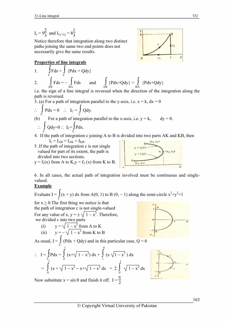
31-Line integral VU
Ic = 923 and Ic1+c2 = 8
13
Notice therefore that integration along two distinct paths joining the same two end points does not necessarily give the same results. Properties of line integrals
1. ∫C Fds = ∫
C {Pdx + Qdy}
2. ∫AB
Fds = − ∫BA
Fds and ∫AB
{Pdx+Qdy} = ∫BA
{Pdx+Qdy}
i.e. the sign of a line integral is reversed when the direction of the integration along the path is reversed. 3. (a) For a path of integration parallel to the y-axis, i.e. x = k, dx = 0
∴ ∫ ∴ ∫(b) For a path of integration parallel to the x-axis, i.e. y = k, dy = 0.
∴ ∫C Qdy=0 ∴ IC=∫
C Pdx.
4. If the path of integration c joining A to B is divided into two parts AK and KB, then Ic = IAB = IAK + IKB.
5 .If the path of integration c is not single valued for part of its extent, the path is divided into two sections. y = f1(x) from A to K,y = f2 (x) from K to B. 6. In all cases, the actual path of integration involved must be continuous and single-
C Pdx = 0 IC =
C Qdy.
valued. Example
Evaluate I = ∫ (x + y) dx from A(0, 1) to B (0, − 1) along the semi-circle x2+y2=1 C
for x > 0.The first thing we notice is that the path of integration c is not single-valued For any value of x, y = ± 1 − x2. Therefore, we divided c into two parts
(i) y = 1 − x2 from A to K (ii) y = − 1 − x2 from K to B
case, Q = 0
∴ I = ∫C Pdx = ∫
1
0 (x+
As usual, I = ∫C (Pdx + Qdy) and in this particular
1 − x2) dx + ∫0
1 (x 1 − x2 ) dx
1
0 = ∫ (x + 1 − x2 − x+ 1 − x2 dx = 2 ∫
1
0 1 − x2 dx
Now substitute x = sin θ and finish it off. I = π2
© Copyright Virtual University of Pakistan
163

31-Line integral VU
for I = 2 ∫1
0 1 − x2dx x = sin θ
∴ dx = cos θ dθ 1 − x2 = cosθ
Limits : x = 0, θ = 0; x = 1, θ = π2
∴ I = 2∫π/2
0 cos2θdθ = ∫
π/2
0 (1+cos2θ)dθ= ⎣⎢
⎡⎦⎥⎤θ +
sin 2θ2
π/2
0 =
π2
Now let us extend this line of development a stage further. Example Evaluate the line integral
I = ∫O (x2dx − 2xy dy) where c comparises the three sides of the triangle joining O(0, 0), A (1, 0) and B (0, 1). First draw the diagram and mark in c1, c2 and c3, the proposed directions of integration. Do just that.The three sections of the path of integration must be arranged in an anticlockwise manner round the figure. Now we deal with each pat separately. (a) OA : c1 is the line y = 0 Therefore, dy = 0.
Then I = ∫O (x2dx − 2xy dy) for this part becomes
I1 = ∫1
0 x2dx = ⎣⎢
⎡⎦⎥⎤x3
3
1
0 =
13 therefore I1 =
13
(b) AB : for c2 is the line y = 1 − x ∴ dy = − dx.
I2 = ∫1
0 {x2dx+2x(1−x)dx}=∫
1
0 (x2+2x−2x2)dx = ∫
1
0 (2x−x2) dx=⎣⎢
⎡⎦⎥⎤x2 −
x3
3
1
0 = −
23
∴ I2 = − 23
Note that anticlockwise progression is obtained by arranging the limits in the appropriate order. Now we have to determine I3 for BO.
∴ I3 = 0
3
(c) BO: c3 is the line x = 0
∴ dx = 0 ∴ I3 = ∫ 0dy = 0
Finally, I = I1+I2+I3 = 1 −
23 + 0 = −
13 ∴ I = −
13
Example
Evaluate ∫Oc
y dx when c is the circle x2+y2 = 4.
x2 + y2 = 4 ∴ y = ± 4 y is thus not single-valued. Therefore use y =
− x2
4 − x2 for ALB between
− x = 2 and x = − 2 and y = 4 − x2 for BMA between = − 2 and x = 2. x
© Copyright Virtual University of Pakistan
164

31-Line integral VU
∴ I = ∫-2
2 I = ∫
-2
2 4 − x2 dx+∫
2
-2 {− 4 − x2 } dx
= 2 ∫-2
2 4 − x2 dx=−2∫
2
-2 4 − x2 dx = − 4 ∫
2
0 4 − x2 dx.
tegral, substitute x = 2 sin θ and finish it off. I = − 4π
To evaluate this in
© Copyright Virtual University of Pakistan
165
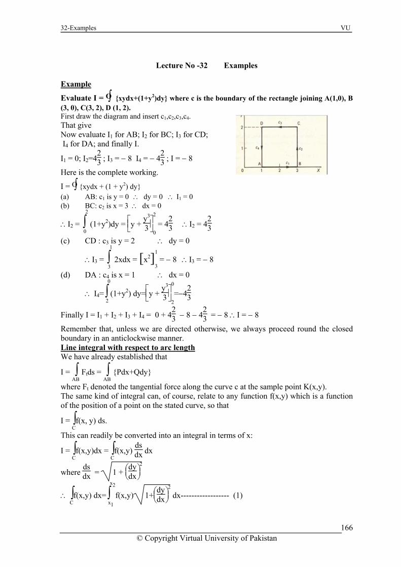
32-Examples VU
Lecture No -32 Examples
Example
Evaluate I = ∫O {xydx+(1+y2)dy} where c is the boundary of the rectangle joining A(1,0), B (3, 0), C(3, 2), D (1, 2). First draw the diagram and insert c1,c2,c3,c4. That give Now evaluate I1 for AB; I2 for BC; I3 for CD; I4 for DA; and finally I.
I1 = 0; I2=423 ; I3 = − 8 I4 = − 4
23 ; I = − 8
Here is the complete working.
I = ∫O {xydx + (1 + y2) dy} (a) AB: c1 is y = 0 ∴ dy = 0 ∴ I1 = 0 (b) BC: c2 is x = 3 ∴ dx = 0
∴I2 = ∫2
0 (1+y2)dy = ⎣⎢
⎡⎦⎥⎤y +
y3
3
2
0 = 4
23 ∴I2 = 4
23
(c) CD : c3 is y = 2 ∴ dy = 0
∫1
[ 2]1− 8
(d) DA : c4 is x = 1 ∴ dx = 0
∴ I4=∫0
2(1+y2) dy=⎣⎢
⎡⎦⎥⎤y +
y3
3
∴I3 = 3
2xdx = x3 = − 8 ∴I3 =
0
2=−4
23
Finally I = I1 + I2 + I3 + I4 = 0 + 423 − 8 − 4
23 = − 8 ∴I = − 8
Re mber that, unless we are directed otherwise, we always proceed round the closed anticlockwise manner.
Line integral with respect to arc length
meboundary in an
We have already established that
ABwhere Ft denoted the tangential force along the curve c at the sample point K(x,y). The same kind of integral can, of course, relate to any function f(x,y) which is a function of the position of a point on the stated curve, so that
I = ∫Cf(x, y) ds.
adily be converted into an integral in terms of x:
I = ∫Cf(x,y)dx = ∫
Cf(x,y)
dsdx
I = ∫AB
Ftds = ∫ {Pdx+Qdy}
This can re
dx
dswhere dx = 1 + ⎝⎜ ⎠⎟
⎞dx
⎛dy 2
∴ ∫Cf(x,y) dx=∫
x2
x1f(x,y) 1+⎝⎜
⎛⎠⎟⎞dy
dx2
dx------------------ (1)
© Copyright Virtual University of Pakistan
166

32-Examples VU
Example
Evalaute I = ∫C(4x+3xy)ds where c is the straight line joining O(0,0) to A (1,2).
c is the line y = 2x ∴ dydx = 2
∴ dsdx = 1 + ⎜⎛ ⎟⎞
dy⎝ ⎠dx
2
= 5
∴ I = ∫x=
(4x+3xy)ds = ∫ (4x+3xy)(x=1 1
0 0 5) dx. But y = 2x
for I = 0
(4x+6x )(∫1
2 5) dx = 2 5 ∫1
0(2x+3x2) dx = 4 5
Parametric Equations When x and y are expressed in parametric form, e.g. x = y (t), y = g(t), then ds dt = ⎝⎜ ⎠⎟dt ∴ ds = ⎝⎜ ⎠⎟dt
⎛ ⎞dx 2 ⎛ ⎞dy + ⎝⎜ ⎠⎟dt
2 ⎛ ⎞dx 2 ⎛ ⎞dy + ⎝⎜ ⎠⎟dt
2
I= ∫Cf(x,y)ds=∫
t2
t1f(x,y)
dt
⎝⎜⎛
⎠⎟⎞dx
dt2 + ⎝⎜
⎛⎠⎟⎞dy
dt2 ----------------(2)
Example
Ev ate I here c is defined as the curve x = sin t, y = cos t between t=0
nd =4
alu = ∫O 4xyds w
tπ
.
t
a
We have x = sin ∴ dxdt = cos t , y = cos t ∴
dydt = − sin t
ds
∴ dt = I
for dtds
= ⎝⎜ ⎠⎟dt⎛ ⎞dx 2 ⎛ ⎞dy
+⎝⎜ ⎠⎟dt2 = cos2 sin2t =1
t2
t+
∴ I = ∫t1
f(x,y) ⎝⎜ ⎠⎟dt⎛ ⎞dx 2 ⎛ ⎞dy
+⎝⎜ ⎠⎟dt2
= ∫π/4
04 sin t cos t dt = 2 ∫
π/4
0sin 2t dt
= − 2 ⎣⎢⎡
⎦⎥⎤cos 2t
2
dt
π/4
0 = 1
Dependence of the line integral on the path of integration We know that integration along two separate paths joining the same two end points does not necessarily give id ntical results.With this in mind, let us investigate the following
eproblem.
© Copyright Virtual University of Pakistan
167

32-Examples VU
EXAMPLE
Evaluate I = ∫OC
{3x2 y2 dx + 2x3y dy} between O (0, 0) and A (2, 4)
(a) along c1 i.e. y = x2
(b) along c2 i.e. y = 2x (c) along c3 i.e. x = 0 from (0,0) to (0,4) and y = 4 from (0,4) to (2,4). (a).First we draw the figure and insert relevant information.
I = ∫C{3x2y2dx + 2x3ydy}
The path c1 is y = x2 ∴ dy = 2x dx
∴ I1 = ∫2
0{3x2x4dx+2x3x22xdx}= ∫
2
0(3x6 + 4x6) dx
∴ = [x7]2
0 = 128 ∴ I1 = 128
) In (b), the path of integration changes to c2, i.e. y = 2x So, in this case,for with c2, y = 2x ∴ dy = 2dx
∴ I2 = ∫2
0(3x2 4x2 dx + 2x3 2x2 dx}
= ∫2
0 20 x4 dx= 4[x5]2
0 = 128 ∴ I2 = 128
(c) In the third case, the path c3 is split
om (0,4) to (2,4) y=4 ∴ dy=0 ∴ I3b=48
∫2
048x2 dx = 128 ∴ I3 = 128
In the example we have just worked through, we took three different paths and in each case, the line integral produced the same result. It appears, therefore, that in this case, the value of the integral is independent of the path of integration taken.
We have been dealing with I = ∫C {3x2y2dx+2x3ydy}
(b
x = 0 from (0,0) to (0, 4), y = 4 from (0, 4) to (2, 4) Sketch the diagram and determine I3. from (0,0) to (0,4) x=0 ∴ dx=0 ∴ I3a=0 fr
© Copyright Virtual University of Pakistan 168

32-Examples VU
Ow
n reflection, we see that the integrand 3x2 y2 dx + 2x3y dy is of the form Pdx+Qdy hich we have met before and that it is, in fact, an exact differential of the function
= x3y2, for ∂z∂xz = 3x2 y2 and
∂z∂y = 2x3 y
This always happens. If the integrand of the given integral is seen to be an exact ifferential, then the value o the line integral is independent of the path taken and depends nly on the coordinates of the two end points.
do
© Copyright Virtual University of Pakistan
169

33-Examples VU
Lecture No -33 Examples Example
Evaluate I = ∫{3ydx + (3x+2y)dy} from A(1, 2) to BC
(3, 5).
No path is given, so the integrand is doubtless an exact differential of some function z = f
(x,y). In fact ∂P∂y = 3 =
∂Q∂x. We have already dealt with the integration of exact
differentials, so there is no difficulty. Compare with
I = ∫C{P dx + Q dy}.
P = ∂z∂x = 3y ∴ z = ∫ 3ydz=3xy+f(y) -------- (i)
Q = ∂z∂y = 3x + 2y ∴ z = ∫(3x+2y) dy = 3xy + y2+F(x) (ii)
For (i) and (ii) to agree f(y) = y2 ; F(x) = 0 Hence z = 3xy + y2
∴I = ∫C{3ydx + (3x+2y)dy}= ∫
(3,5)
(1,2)d(3xy+y2)=[3xy+y2]
(3,5)
(1,2) = (45+25) − (6+4) = 60
Example
Evaluate I = ∫C{(x2+yex)dx+(ex+y)dy} between A (0, 1) and B (1, 2).
As before, compare with ∫C {Pdx+Q dy}.
P = ∂z∂x =x2+yex ∴ z =
x3
3 + yex+f (y)
Q = ∂z∂y =ex+y ∴ z = yex +
y2
2 + F(x)
For these expressions to agree, 2
f(y) = y2 ; F(x) = 3
x3
Then I = ⎣⎢⎡
⎦⎥⎤x3
3 + yex + y2
2
(1,2)
(0,1) =
56 + 2e
So the m in points are that, if (Pdx+Qdy) is an exact differential
(a) I = ∫(Pdx + Qdy) is independent of the path of integration
(b) I = ∫O (P dx + Q dy) is zero.
If I = ∫{P dx + Q dy} and (Pdx + Qdy) is an exact differential,
Ic1 + Ic2 = 0 ro,
Q dy) = 0
a
C
C
C Then Ic1 = Ic2
Hence, the integration taken round a closed curve is ze provided (Pdx+Q dy) is an exact differential.
∴ If (P dx + Q dy) is an exact differential, ∫O (P dx +
© Copyright Virtual University of Pakistan
170

33-Examples VU
Exact differentials in three independent variables olves three independent variables, but the method is
ery much like that for two independent variables. exact differential of z = f(x, y, w)
if ∂
A line integral in space naturally invvdz = Pdx + Q dy + R dw is an
∂Py = ∂x
∂Q ; ∂w
∂P = ∂x
∂R ; ∂y
∂R = ∂w
∂Q
If the test is successful, then
(a) ∫C (P dx + Q dy + R dw) is independent of the path of integration.
(b) ∫OC
(P dx + Q dy + R dw) is zero.
Example Verify that dz=(3x2yw+6x)dx+(x3w−8y)dy+(x3y+1) dw is inexact differential and hence
evaluate ∫C dz from A (1, 2, 4) to B (2, 1 3).
First check that dz is an exact differential by finding the partial derivatives above, when P = 3x2yw + 6x; Q = x3w − 8y; and R = x3y + 1 ∂P∂y = 3x2w ;
∂Q∂x = 3x2w ∴
∂Py∂ =
∂Q∂x
∂w∂P
= 3x2y ; ∂x∂R
= 3x2y ∴ P
∂w∂
= ∂R∂x
∂R∂y = x3;
∂Q∂w = x3 ∴
∂R∂y =
∂Q∂w
∴ dz is an exact differential
Now to find z. P = ∂z∂x ; Q =
∂z∂y ; R =
∂z∂w
∴ ∂z∂x =3x2yw+6x ∴ z=∫(3x2yw+6x)dx = x3yw+3x2+f(y)+F(w)
∴ ∂z∂y =x3w−8x ∴ z = ∫(x3w−8y)dy = x3yw−4y2+g(x)+F(w)
∂w ∂z
=x3y+1 ∴ z = ∫(x3y+1)dw = y3yw+w+f(y)+g(x)
For these three expressions for z to agree f(y) = − 4y2; F(w) = w; g(x) = 3x2
∴ z = x3yw + 3x2 − 4y2 + w
∴ I = [x3yw + 3x2−4y2+w](2,1,3)
(1,2,4)
2− 2 ](2,1,3)
− −(8+3−16+4)=36
ightforward. Finally, we have a theorem that can be very helpful on occasions and which links up with
s start a new section.
for I = [x3yw + 3x 4y +w(1,2,4)
= (24+12 4+3)
The extension to line integrals in space is thus quite stra
the work we have been doing. It is important, so let u
© Copyright Virtual University of Pakistan
171

33-Examples VU
Green’s Thorem Let P and Q be two function of x and y t and continuous inside and the boundary
hat are finite c of a region
then Green’s theorem states that.
∫R∫⎝⎜⎛
⎠⎟⎞∂P
∂y
R in the xy-plane.If the first partial derivatives are continuous within the region and on the boundary,
− ∂Q∂x dx dy = − ∫O
C (P dx+ Q dy)
That is, a double integral over the plane region R can be transformed into a line integral over the boundary c of the region – and the action is reversible. Let us see how it works.
EXAMPLE
The integ s e form
C ∂y
Evaluate I = ∫O {(2x − y)dx + (2y+x)dy} around the boundary c . the ellipse C
x2 + 9y2 = 16. ral i of th
I = ∫O {P dx + Q dy) where P = 2x − y ∴ ∂P
= − 1 and Q = 2y + x ∴ ∂Q∂x = 1.
∴ I =−∫R∫⎝⎜⎛
⎠⎟⎞∂P
∂y−∂Q∂x dxdy=−∫
R∫(−1−1)dx dy= 2 ∫
R∫dx dy
16
But ∫R∫dx dy over any closed region give the area of the figure.
In this case, then, I = 24 where A is the area of the ellipse
x2+9y2 = 16 i.e. x2
+9y2
16 = 1
∴ a = 4; b =4 3 ∴ A =
16π3 ∴ I = 2A =
32π3
lying Green’s theorem. Example
To demonstrate the advantage of Green’s theorem, let us work through the next example (a) by the previous method, and (b) by app
valuate I = ∫OC
{(2x+y) dx+(3x−2y) dy} taken in anticlockwise manner round the triangle
ith vertices at O (0,0) A (1, 0) B (1, 2).
= ∫OC
{(2x + y) dx + (3x − 2y) dy}
E
w
I
© Copyright Virtual University of Pakistan
172

33-Examples VU
(a) By the previous method There are clearly three stages with c1,c2,c3. Work through the complete evaluation to determine the value of I. It will be good revision. When you have finished, check the result with the solution in the next frame. I = 2 (a) (i) c1 is y = 0 ∴ dy = 0
∴ I1 = ∫1
02x dx = [x2]
1
0 = 1 ∴ I1 = 1
(ii) c2 is x = 1 ∴ dx = 0
∴ I2=∫2
0(3−2y) dy=[3y−y2]
0
1 =2 ∴ I2=2
(iii) c3 is y = 2x ∴ dy = 2 dx
I3 = ∫0
{4x dx + (3x − 4x) 2 dx}
= ∫ 2x dx = [x2] = − 1 ∴ I3 = − 1
+I +I = 1+2+( 1) = 2 ∴ I = 2
Now we will do the same problem by applying Green’s theorem, so more (b) By Green’s theorem
I = ∫OC
{(2x + y) dx + (3x − 2y) dy}
P = 2x + y ∴ ∂P∂y
∴10
0
1 1
I = I −1 2 3
=1;
Q = 3x − 2y ∴ ∂Q∂x = 3
I = − ∫R∫⎝⎜⎛
⎠⎟⎞∂P
∂y − ∂Q∂x dx dy
= 2 × the area of the triangle = 2 × 1 = 2
ays the quickest method. It is useful, however, have both methods available.
⎝ ⎠∂y
Finish it off. I = 2
For I = − ∫∫(1−3) dx dy=2 ∫∫dx dR R
y = 2A
∴ I = 2 Application of Green’s theorem is not alwtoIf you have not already done so, make a note of Green’s theorem.
∫∫⎜⎛
⎟⎞∂P
− ∂Q∂x dx dy = − ∫O (P dx + Q dy)
R C
ote: Green’s theorem can, at is not simply connected by arranging a link between o ded the path of integration is such that the region is kept on the left-hand side.
N in fact, be applied to a region th
uter and inner boundaries, provi
© Copyright Virtual University of Pakistan
173

34-Examples VU
Lecture -34………Examples Example
C − y) dy} round the region bounded by
2 2 by the use of Green’s theorem. , 0) and A(1, 1).
x
C R ⎝∂y
Evaluate the line integral I = ∫O {xy dx + (2x
the curves y = x and x = yPoints of intersection are O(0
I = ∫O {xy dx + (2 − y) dy} C
∫O {Pdx+ Qdy}= −∫∫⎜⎛
⎟⎞∂P⎠
− ∂Q
dx dy ∂x
P = xy ∴ ∂P∂y = x; Q = 2x − y ∴
∂Q∂x =2
I = − ∫R∫ (x − 2) dx dy = − ∫
1
0∫
y=√x
y=x2(x − 2) dy dx
= − ∫1
0 (x − 2) [ y ]
√x
x2 dx
0 − (∴ I = − ∫
1
(x 2) ) x x2 dx = −∫1
−0
(x3/2 − x3 − 2x1/2 + 2x2) dx
⎣ ⎦5 = − ⎢⎡ ⎥⎤2 x5/2−
14x4 −
43x3/2+
23x3
1
= 3160
0
In this special case when P=y and Q= x so ∂y−∂P
= 1 and ∂x∂Q
= − 1
Green’s theorem then states ∫R∫{1 − (−1)} dx dy =− ∫O
C (P dx+Q dy)
i.e. 2 ∫R∫dx dy = − ∫O
C (y dx − x dy) = ∫O
C (x dy − y dx)
Therefore, the area of the closed region A = ∫R∫dx dy =
12 ∫O
C (x dy − y dx)
Example Determine the area of the figure enclosed by y = 3x2 and y = 6x.
oints of intersection : 3x2 = 6x ∴ x = 0 or 2
Area A = 12
P
∫OC
(x dy − y dx)
We evaluate the integral in two parts, i.e. OA along c1 and AO along c2
2A=∫c1
(xdy−ydx)(along OA)
+∫c2
(xdy−ydx)(along OA)
= I1+I2
I1: c1 is y = 3x2 ∴ dy = 6x dx
© Copyright Virtual University of Pakistan
174

34-Examples VU
∴ I1 = ∫2
0(6x2dx − 3x2dx) = ∫
2
0 3x2 dx = [ x3 ]
2
0 = 8 ∴ I1 = 8
Similarly, for c2 is y = 6x ∴ dy = 6 dx
∴ I2 = ∫0
2(6x dx − 6x dx) = 0
∴ I2 = 0 ∴ I = I1 + I2 = 8 + 0 = 8 ∴ A = 4 square units Example Determine the area bounded by the curves y = 2x3, y = x3 + 1 and the axis x = 0 for x > 0. Here it is y = 2x3; y = x3 + 1; x = 0 Point of intersection 2x3 = x3 + 1 ∴ x3 = 1 ∴ x = 1
Area A = 12 ∫O
C (x dy − y dx) ∴ 2A = ∫O
C (x dy − y dx)
(a) OA : c1 is y = 2x3 ∴ dy = 6x2 dx
∴I1=∫c1
(xdy −ydx)=∫1
0(6x3dx−2x3 dx) = ∫
1
04x3 dx = [ x4 ]
1
0 = 1
∴ I1 = 1 (b) AB: c2 is y = x3 + 1 ∴ dy = 3x2 dx
∴ I2 = ∫0
1 {3x3 dx − (x3 + 1) dx} = ∫
0
1(2x3 − 1) dx = ⎣⎢
⎡⎦⎥⎤x4
2 − x0
1 = − ⎝⎜
⎛⎠⎟⎞1
2 − 1 = 12
∴ I2 = 12
(c) BO: c3 is x = 0 ∴ dx = 0 y=0
0
∴ 2A = I = I1 + I2 + I3 = 1 + 12
I =∫ (xdy − ydx)=0 ∴ I3y=1
3 =
+ 0 = 112 ∴ A =
34 square units
Revision Summary Properties of line integrals
• Sign of line integral is reversed when the direction of integration along the path
∫ Q dy.
• ration parallel to x-axis, dy = 0 ∴ Ic = ∫c P dx.
s and single-valued. • f integration.
value of the line integral depends on the particular path of integ n.
If P dx + Q dy is an exact differential
is reversed.
• Path of integration parallel to y-axis, dx = 0 ∴ Ic =c
Path of integ
Path of integration must be continuouDepen nce line integral on path o
•de of
• In general, the tiora
• Exact differential
© Copyright Virtual University of Pakistan
175

34-Examples VU
(a) ∂P∂y =
∂Q∂x
(b) I = ∫c (P dx + Q dy) is independent of the path of integration
(c) I = ∫OC
(P dx + Q dy) is zero.
• Exact differential in three variables. If P dx + Q dy + R dw is an exact differential
(a) ∂P∂y =
∂Q∂x ;
∂P∂w =
∂R∂x ;
∂R∂y =
∂Q∂w
c
+ R dw) is independent of the path of integration.
(c) ∫O (P dx + Q dy + R dw) is zero.
∫OC
(P dx+Q dy)=− ∫R∫
⎩⎪⎨⎪⎧
⎭⎪⎬⎪⎫∂P
∂y
(b) ∫ (P dx + Q dy
C
• Green’s theorem
− ∂Q∂x dx dy and, for a simple closed curve,
∫OC
(x dy − y dx) = 2 ∫R∫dx dy = 2A
where A is the area of the enclosed figure. Gradient of a scalar function
Del operator is given by ∇ = ⎝⎜⎛
⎠⎟⎞i
∂∂x + j
∂∂y+ k
∂∂z
∇φ = grad φ = ⎝⎜⎛
⎠⎟⎞i
∂∂x + j
∂∂y+ k
∂∂z φ = i
∂φ∂x + j
∂φ∂y + k
∂φ∂z
gradφ = ∇φ = ∂φ∂x i +
∂φ∂y j +
∂φ∂z k
Div (Divergence of a vector function)
then div A = ∇.A = ⎝⎜⎛
⎠⎟⎞i
∂∂x
If A = a1i + a2j + a3k
+ j∂∂y+ k
∂∂z .(a1i + a2j + a3k)
∴ div A = ∇.A = ∂a1
∂x +∂a2
∂y +∂a3
∂z
Note that (a) the grad operator ∇ acts on a scalar and gives a vector (b) the div operator ∇. acts on a vector and gives a scalar. Example If A = x2yi − xyzj + yz2k then
Div A = ∇.A = 2 4( ) ( ) ( )x y xyz yzx y z
∂ ∂ ∂− +
∂ ∂ ∂= 2xy − xz + 2yz
Example
© Copyright Virtual University of Pakistan
176

34-Examples VU
If A = 2x2yi − 2(xy2+y3)j+3y2z2k determine ∇.A i.e. div A. A= 2x2yi − 2(xy2 + y3z)j + 3y2z2k
∂a∇.A= x
∂x + y
∂y∂a
+ z
∂z∂a
= 4xy−2(2xy+3y2z)+6y2z= 4xy − 4xy − 6y2z+6y2z = 0
Such a vector A for which ∇.A = 0 at all points, i.e. for all values of x, y, z, is called a solenoid vector. It is rather a special case. Curl (curl of a vector function) The curl o acts on a vector and gives another vector as a result.
A.
i.e. curl A⎠⎟
perator denoted by ∇×, If A= a1i + a2j + a3k then curl A=∇×
=∇×A= ⎝⎜⎛ ⎞i
∂∂x + j
∂∂y+ k
∂∂z × (a1i + a2j + a3k)
=
⎪⎪ ⎪⎪∂x
⎪⎪ ⎪⎪ i j k∂
∂y∂
∂z∂
a1 a2 a3
∴ ∇×A= i ⎝⎜⎛
⎠⎟⎞∂a3
∂y − ∂a2
∂z +j ⎝⎜⎛
⎠⎟⎞∂a1
∂z − ∂a3
∂x + k ⎝⎜⎛
⎠⎟⎞∂a2
∂x − ∂a1
∂y
Curl A is thus a vector function. Example If A=(y4−x2z2)i+(x at the point (1,3, −2).
⎪ ⎪
⎪j k
2+y2)j−x2yzk,determine curl A
Curl A = ∇ × A = ⎪⎪
⎪⎪
∂∂x
⎪ i
∂
∂y ∂∂z
y4−x2z2 x2+y2 −x2yzNow we expand the determinant
∇ × A= i ⎩⎪⎨⎪⎧
⎭⎪⎬⎪⎫∂
∂y (− x2yz) − ∂∂z (x2+y2) − j
⎩⎪⎨⎪⎧
⎭⎪⎬⎪⎫∂
∂x (− x2yz) − ∂∂z (y4 − x2z2)
+ k ⎩⎪⎨⎪⎧
⎭⎪⎬⎪⎫∂
∂x (x2 + y2) − ∂∂y (y4 − x2z2)
∇×A=i{−x2z}−j{−2xyz+2x2z}+k(2x−4y3}. ∴ At (1, 3, − 2), ∇×A = i (2)−j (12 − 4) + k (2 − 108) = 2i − 8j − 106k Example Determine curl F at the point (2,0,3) given that F=ze2xyi+2xycosyj+(x+2y)k.
In determine form, curl F = ∇ × F =
⎪⎪⎪⎪
⎪⎪⎪⎪
i j k
∂∂x
∂∂y
∂∂z
ze2xy 2xzcosy x+2y
Now expand the determinant and substitute the values for x, y and z, finally obtaining curl
× F = i{2 − 2x cos y}− j{1 − e2xy}+ k ({2z cos y − 2xze2xy} ∇× − − − − − − −
∇∴At(2,0,3) F= i(2 4) j(1 1)+k(6 12) = 2i 6k = 2 (i + 3k)
Summary of grad, div and curl
© Copyright Virtual University of Pakistan
177

34-Examples VU
(a) Grad operator ∇ acts on a scalar field to give a vector field. (b) Div operator ∇. Acts o a vector field to give a scalar field. (c) Curl operator ∇ × acts on a vector field to give a vector field.
Grad φ = ∇φ ∂x
(d) With a scalar function φ (x,y,z)
= ∂φ
i+∂y∂φ
j+∂z∂φ
k
(e) With a vector function A=axi+ayj+azk
(i) div A = ∇.A= ∂ax
∂x + ∂ay
∂y + ∂az
∂z
(ii) Curl A = ∇ × A =
⎪⎪⎪⎪
⎪⎪⎪⎪
i j k∂∂x
∂∂y
∂∂z
ax ay az
Multiple Operations We can combine the operators grad, div and curl in multiple operations, as in the examples that follow. EXAMPLE If A = x2yi + yz3j − zx3k
Then div A=∇.A = ⎝⎜⎛
⎠⎟⎞i
∂∂x + j
∂∂y+ k
∂∂z .(x2yi + yz3j − zx3k)
= 2xy+z3 + x3 = φ (say)
Then grad (div A) = ∇(∇.A) = ∂φ∂x i +
∂φ∂y j +
∂φ∂zk = (2y+3x2)i+(2x)j+(3z2)k
i.e., grad div A = ∇(∇.A)= (2y+3x2)i+2xj+3z2k
Example If φ = xyz − 2y2z + x2z2 determine div grad φ at the point (2, 4, 1). First find grad φ and then the div of the result. div grad φ = ∇.(∇φ) We have φ = xyz − 2y2z + x2z2
grad φ = ∇φ = ∂φ∂x i +
∂φ∂y j + ∂
∂φz k =(yz+2xz2)i+(xz−4yz)j+(xy−2y2+2x2z) k
2
∂φ
∴ div grad φ=∇.(∇φ) = 2z − 4z+2x2
∴ At (2,4,1), div grad φ = ∇.(∇φ) = 2 − 4 + 8 = 6
grad φ = ∂x i + ∂y∂φ
j + φ
∂z∂
k
Then div grad φ = ∇.(∇φ)= ⎝⎜⎛
⎠⎟⎞i
∂∂x + j
∂∂y+ k
∂∂z .⎝⎜
⎛⎠⎟⎞∂φ
∂x i+∂φ∂y j+
∂φ∂z k =
∂2φ∂x2 +
∂2φ∂z2 +
∂2φ∂z2
∴div grad φ=∇.(∇φ) = ∂2φ∂x2+
∂2φ∂y2+
∂2φ∂z2
© Copyright Virtual University of Pakistan
178

34-Examples VU
Example If F = x2yzi + xyz2j + y2zk determine curl F at the point (2, 1, 1).Determine an expression for curl F in the usual way, which will be a vector, and then the curl of the result. Finally substitute values. Curl curl F=∇×(∇×F) = i+2j+6k
For curl F =
⎪⎪⎪⎪
⎪⎪⎪⎪
i j k
∂∂x
∂∂y
∂∂z
x2yz xyz2 y2z
= (2yz−2xyz)i+x2yj+(yz2−x2z)k
⎪⎪
⎪⎪⎪⎪
i j k∂
Then Curl Curl F = ⎪ ∂x
⎪
∂∂y
∂∂z
2yz−2xyz x2y yz2−x2z
= z2i−(−2xz− 2y+2xy)j+(2xy−2z+2xz)k
∴ At (2, 1, 1), curl cul F=∇×(∇ × F) = i + 2j + 6k Two interesting general results (a) Curl grad φ where φ is a scalar
grad φ = ∂φ∂x i +
∂φ∂y j +
∂φ∂z k
∴ curl grad φ =
⎪⎪⎪
⎪⎪⎪i j k
∂∂x
∂∂y
∂∂z
∂φ∂x
∂φ∂y
∂φ∂z
= i ⎩⎪⎨⎪⎧
⎭⎪⎬⎪⎫∂2φ
∂y∂z − ∂2φ
∂z∂x − j ⎩⎪⎨⎪⎧
⎭⎪⎬⎪⎫∂2φ
∂z∂x − ∂2φ
∂x∂z + k ⎩⎪⎨⎪⎧
⎭⎪⎬⎪⎫∂2φ
∂x∂y − ∂2φ
∂y∂x = 0
∴ curl grad φ = ∇ × (∇φ) = 0 (b) Div curl A where A is a vector. A = axi + ayj + azk
curl A = ∇ × A=
⎪⎪⎪⎪
⎪⎪⎪⎪
i j k∂∂x
∂∂y
∂∂z
ax ay az
= i⎝⎜⎛
⎠⎟⎞∂az
∂y − ∂ay
∂z − j ⎝⎜⎛
⎠⎟⎞∂az
∂x − ∂ax
∂z + k ⎝⎜⎛
⎠⎟⎞∂ay
∂x − ∂ax
∂y
Then div curl A = ∇.(∇×A) = ⎝⎜⎛
⎠⎟⎞i
∂∂x + j
∂∂y+ k
∂∂z . (∇ × A)
= ∂2az
∂x∂y − ∂2ay
∂z∂x − ∂2az
∂x∂y +∂2ax
∂y∂z − ∂2ay
∂z∂x − ∂2ax
∂y∂z = 0
∴ div curl A = ∇ . (∇ × A) = 0 (c) Div grad φ where φ is a scalar.
grad φ = ∂φ∂x i +
∂φ∂y j +
∂φ∂z k
Then div grad φ = ∇.(∇φ)= ⎝⎜⎛
⎠⎟⎞i
∂∂x + j
∂∂y+ k
∂∂z .⎝⎜
⎛⎠⎟⎞∂φ
∂x i+∂φ∂y j+
∂φ∂z k =
∂2φ∂x2 +
∂2φ∂z2 +
∂2φ∂z2
∴div grad φ=∇.(∇φ) = ∂2φ∂x2+
∂2φ2∂y +
∂2φ∂z2
This result is sometime 2φ. s denoted by ∇So these general results are
© Copyright Virtual University of Pakistan
179

34-Examples VU
(a) curl grad φ = ∇×(∇φ) = 0 ) div curl A = ∇.(∇×A) = 0
) div grad φ=∇.(∇φ)=∂2φ∂x2
(b
(c +∂2φ∂y2+
∂2φ∂z2
© Copyright Virtual University of Pakistan
180

35-Definite intagrals VU
Lecture No -35 Definite Integrals
efinite integral for sin D nx and cosnx , 0 ≤ x ≤ π/2
-------------------------------------------------
-------------------------------------------------
2 2 22
00 0
22
0
1 1 sin 2 1 sinn (1 cos 2 )2 2 2 2 2 2 4
1sin
2 2
xxdx x dx x
xdx
π π π
π
si
π π π
π
== − = − = −
=
∫ ∫
∫
2 2 22
0 0
22
0
1 1 sin 2 1 sins (1 cos 2 )2
1cos
2 2
xxdx x dx x
xdx
π π π
π
co02 2 2 2 2 4
π π π
π
= + = + = + =
=
∫ ∫
∫
2 2 2 2 23 2 2 2
0 0 0 0 0
3 23 32
00
2 2 23 2 2 2
0 0
n sin sin (1 cos )sin sin cos ( sin )
cos 1 1 2cos cos cos 0 cos cos 0 13 2 3 2 3 3
cos cos cos (1 sin )cos cos sin (co
si
0
xdx x xdx x xdx xdx x x dx
xx
xdx x xdx x xdx xdx x
π π π π π
ππ
π π π
π π
= = − = + −
⎡ ⎤= − + = − + + − = − =⎢ ⎥⎣ ⎦
= = − = −
∫ ∫ ∫ ∫ ∫
∫ ∫ ∫2 2
3 23 32
00
s )
sin 1 1 2sin sin sin 0 sin sin 0 13 2 3 2 3 3
0 0
x dx
xx
π π
ππ π π⎡ ⎤= − = − − − = − =⎢ ⎥⎣ ⎦
∫ ∫
22 2 24 2 2 2
0 0 0
2 2
0 0
2
0
1 cos 2 1n (sin ) (1 2cos 2 cos 2 )2 4
1 1 cos 4 1 3 os 4(1 2cos 2 ) ( 2cos 2 )4 2 4 2 2
1 3 sin 4 1 3 sin 2sin 2 sin4 2 8 4 2 2 8
4 2 2
x
2
si0
24 1 3sin
0
xdx x dx dx x x dx
x c xx dx x dx
xx x
π π π
π π
π
π ππ
−⎡ ⎤= = = − +⎢ ⎥⎣ ⎦
+= − + = − +
⎡ ⎤= − + = − +⎢ ⎥⎣ ⎦
⎣ ⎦
∫ ∫ ∫ ∫
∫ ∫
π
π2
4 3 sinso xdx =∫0
1 4 2 2
π
πxdx π⎡ ⎤= ⎢ ⎥∫
© Copyright Virtual University of Pakistan
181
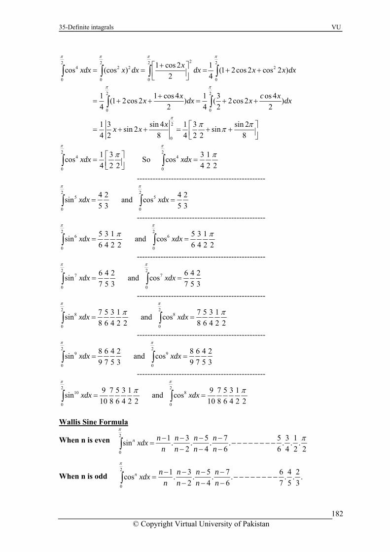
35-Definite intagrals VU
22 24 2 2 2
0 0
2 2
0 0
2
0
24
0
1 cos 2 1cos (cos ) (1 2cos 2 cos 2 )2 4
1 1 cos 4 1 3 os 4(1 2cos 2 ) ( 2cos 2 )4 2 4 2 2
1 3 sin 4 1 3 sin 2sin 2 sin4 2 8 4 2 8
1 3cos4 2 2
x
-------------------------------------------------
2 25 5 4 2cos xdx =∫
0 0
4 2sin and5 3 5 3
xdx
π
=∫-------------------------------------------------
π
2 26 6 5 3 1and cos
6 4 2 2xdx
0 0
5 3 1sin 6 4 2 2
xdx
π π
π π∫ = =∫
-------------------------------------------------
2 27 7
0 0
6 4 2 6 4 2sin and cos7 5 3 7 5 3
xdx xdx
π π
= =∫ ∫
-------------------------------------------------
2 28 8
0 0
7 5 3 1 7 5 3 1sin and cos8 6 4 2 2 8 6 4 2 2
xdx xdx
π π
π π= =∫ ∫
-------------------------------------------------
2 29 9
0 0
8 6 4 2 8 6 4 2sin and cos9 7 5 3 9 7 5 3
xdx xdx
π
= =∫ ∫
-------------------------------------------------
π
2 210 8
0 0
9 7 5 3 1 9 7 5 3 1sin and cos10 8 6 4 2 2 10 8 6 4 2 2
xdx xdx
π π
π π= =∫ ∫
Wallis Sine Formula
When n is odd
When n is even
2 2
0 0
2
xdx x dx dx x x dx
x c xx dx x dx
xx x
xdx
π π
π π
π
π
π ππ
π
+⎡ ⎤= = = + +⎢ ⎥⎣ ⎦
+= + + = + +
⎡ ⎤= + + = + +⎢ ⎥⎣ ⎦
⎡ ⎤= ⎢ ⎥⎣ ⎦
∫ ∫
∫ ∫
∫
π π
∫ ∫
24
0
3 1 So cos 4 2 2
xdx
π
π=∫
2
0
1 3 5 7 5 3 1. . . . . . .2 4 6 6 4 2 2
n n n n nxdxn n n n
π
π− − − −= − − − − − − − −
− − −∫ sin
2
0
1 3 5 7 6 4 2cos . . . . . . .2 4 6 7 5 3
n n n n nxdxn n n n
π
− − − −= − − − − − − − −
− − −∫
© Copyright Virtual University of Pakistan
182

35-Definite intagrals VU
2 211 11
0 0
10.8.6.4.2 10.8.6.4.2sin and cos11.9.7.5.3 11.9.7.5.3
xdx xdx
π π
= =∫ ∫
2 212 12
0 0
11.9.7.5.3.1 11.9.7.5.3.1sin and cos10.8.6.4.2 2 10.8.6.4.2 2
xdx xdx
π π
π π= =∫ ∫
Integration By Parts
dU dx.UVdx U V dx Vdxdx
⎡ ⎤= − ⎢ ⎥⎣ ⎦∫ ∫ ∫ ∫
Example x lnx dx Evaluate ∫
∫ x lnx dx= lnx ∫ xdx – [∫ ∫ x dx. ddx
(ln x)] dx (We are integrating by parts)
= ln x(2
2x )- ∫ (
2
2x )( 1
x)dx=(
2
2x ) ln x- ∫ (
2x )d x = (
2
2x ) ln x- 1
2 (
2
2x )
© Copyright Virtual University of Pakistan 183
Example Eva x sinx dx luate ∫
∫ x sinx dx =x ∫ sin xdx – ∫ [ ∫ sinx dx. d (x)]dx
dx (We are integrating by parts)
= x(-cosx)- (-cosx)(1)dx= -x(cosx ) +∫ ∫ cosx d x = -x(cosx)+sin x Line Integrals
by the position vector r with respect to origin O. If q is a neighboring point on the curve with position vector
r+dr , then
Let a point p on the curve c joining A and B be denoted
PQ = r The curve c can be divided up into many n such small arcs , approximating to dr1 , dr2 , dr3 ,………. drp ,……
so that 1
n
pp
AB dr∑ where dr is a vector representing the element of the arc in bo=
p th
. magnitude and direction. If dr → 0 , then the length of the curve AB=c
dr∫Scalar Field If a scalar field V(r) exists for all points on the curve ,
the 1
pp=
( )n
V r dr∑ with dr → 0 , defines the line integral
of V i.e line integral =
We can illustrate this integral by erecting a continuous Ordinate to V(r) at each point of the curve is then represented by the area of the
curved surface between the ends A and B the curve c. To evaluate a line integral , the integrand is expressed in terms of x , y ,z with dr =dx + dy j + dz k In practice , x , y and are often expressed in terms of parametric equation of a fourth variable (say u), i.e. x = x(u) ; y = y(u) ; z = z(u) . From these , dx, dy and dz can be written in terms of u and the integral evaluate in terms of this parameter u.
( ) .c
V r dr∫
( )c
V r dr∫

36-Scalar field VU
Lecture No -36 Scalar Field Scalar Field If a scalar field V(r) exists for all points on the curve ,
the V r dr∑ with dr → 0 , defines the line integral
We can illustrate this integral by erecting a continuous Ordinate to V(r) at each point of the curve is then represented by the area of the
curved surface between the ends A and B the curve c. To evaluate a line integral , the integrand is expressed in terms of x , y ,z with dr =dx + dy j + dz k In practice , x , y and are often expressed in terms of parametric equation of a fourth
z = z(u) . From these , dx, dy and dz can be rms of u and the integral evaluate in terms of this parameter u.
Example
1p=
( )n
p
of V i.e line integral = ( ) .c
V r dr∫
( )c
V r dr∫
variable (say u), i.e. x = x(u) ; y = y(u) ; written in te
V=xy2z , evaluate along the curve c having parametric equations
x = 3u; y=2u2 ;z=u3 between A(0,0,0) and B(3,2,1) V= xy2z = (3u)(4u4)(u3)=12u8
dr= dxi+ dy j+ dz k ⇒ dr= 3du i +4udu j +3u2du k r x = 3u ; ∴ dx = 3du ; y = 2u2 ∴ dy = 4u du ; z = u3 ∴ dz =3u2dz imiting : A(0,0,0) corresponds to B(3,2,1) corresponds to u
A(0,0,0) ≡ u=0 ; B(3,2,1) ≡ u = 1
( )c
V r dr∫ If
foL
11 9 10 118 2
0 0
u 2( ) 12u (3 i +4u j +3u k)du= 36 48 36 49 10 11 5 1c
u uV r dr i j i j k= + +∫ ∫ 4 361
= + +
Example If V = xy + y2z Evaluate along the curve c defined by x= t2; y = 2t ; z= t+5
between A(0,0,5) and B(4,4,7) . As before , expressing V and dr in term of the parameter t .
( )c
V r dr∫
since V=xy+y 2z = (t2 )(2t)+(4t2 )(t+5) = 6t3 + 20t2.
x = t2 dx = 2t dty = 2t dy = 2 dt z = t+5 dz = dt
} ∴ dr = dxi
+ dy j + dzk = 2t dt i + 2 d t j + dtk ∴ ∫
C Vdr = ∫
C (6t3 +20t2)( 2t i + 2 j+k) dt
© Copyright Virtual University of Pakistan
184

36-Scalar field VU
Limits: A (0, 0, 5) ≡ t = 0; B (4, 4, 7) ≡ t = 2
∴ ∫
© Copyright Virtual University of Pakistan 185
C 0 Vdr = ∫ (6t +20t )( 2t i +2 j +k) dt
23 2
∫C 0
+203
Vdr = 2 ∫ {6t4 t3)i+(6t3+20t2)j
+(3t +10t2)k}dt.
= 815
2
(444i + 290j + 145k)
Vector Field t for all points of the curve c, then for each element of arc we can
form the scalar product F.dr. Summing these products for all elements of arc, we have
F= F1 i + F2 j +F3 k And dr = dx i +dy j +dz k Then F.dr = (F1 i + F2 j +F3 k).( dx i +dy j +dz k) =
Now for an example to show it in operation. Example
If a vector field F(r) exis
1
.n
pp
F dr=
∑
1 2 3(Fdx + F dy +F dz )c∫
If F(r) = x2y i + xz j + 2yz k , Evaluate .
c
F dr∫ between A(0,0,0) and B(4,2,1) along the
urve c having parametric equations x=4t ; y-2t2; z = t3
Expressing everthing in terms of the parameter t, we have dx = 4 dt ; dy =4tdt ; dz = 3t2 dt x2y = (16t2)(2t2) = 32 t 4
x = 4t ∴ dx = 4 dt xz = (4t)(t3) = 4 t4
y = 2 t 2 dy = 4t dt 2yz = (4 t 2)( t 3) = 4 t 5
z = t 3 ∴ dz = 3t2 dt F = 32 t 4 i + 4 t4 j – 4 t5 k dr = 4dt i + 4t dt j + 3t2 k
T he line integral of F(r) fr om A to B along the stated curve = ∫
C F.dr.
In this case, since F.d r is a scalar p
c
roduct, then the line integral is a scalar. To evaluate the line integral, F and d r are expressed in terms of x,y,z, and the curve in parametric form. We have
Then ∫ F. d r = ∫ (32t4 i+4t4j− 4t5 k). (4dt i + 4t dt
j + 3t2 dt k)
= ∫ (128t4+16t5 + 12t7) dt its: A(0,0,0) ≡ t = 0;
B (4, 2, 1) ≡ t = 1 ∫C F. d r = (128
Lim
t4 + 16t 5 + 12t7)dt = 1285 t5 +
166 t6 +
128 t8 =
1285 +
83 +
3 2 = 29.76

36-Scalar field VU
Example
f I
F(r ) = x2y i + 2yzj + 3z2 x k valuate ∫
C F. d r between A(0,0,0) and B(1,2,3)
B (1, 2, 3) (a) along the straight line c1 from (0, 0, 0) to (1, 0, 0) then c2 from (1, 0, 0) to (1, 2, 0) and c3 from (1, 2 , 0) to (1, 2, 3)
E
(b) along the straight line c 4 joining (0, 0, 0) to (1, 2, 3). W e first obtain an expression for F.dr which is F. d r = (x2y i + 2yzj + 3z2x k).
(dx i+ dy j + dz k) F. d r = x2 y dx + 2yz dy + 3z 2 x dz
∫ F.d r = ∫ x 2 ydx + ∫2yzdy+∫ 3z 2xdz Here the integration is made in threesections, along c 1 , c 2 and c 3 .
(i) c1 : y = 0, z = 0, dy = 0, dz = 0 ∴ ∫
C1 F. d r=0+0+0 = 0
e conditions along c 2 are c 2: x = 1, z = 0, dx = 0, dz = 0
∴ ∫ C2
F.dr = 0 + 0 + 0 = 0
3 : x = 1, y = 2, dx = 0, dy = 0
∫3 F. dr = 0 + 0 + ∫
3
0 3z 2dz = 27
Summing the three partial results
∫( 1 , 2 , 3)
( 0 , 0 , 0 ) F.d r = 0 + 0 + 27 = 27
∴ ∫ c 1+c 2+ c 3
F. d r = 27
(ii) c2 : Th
(iii) c
C
If
t taken as the parameter, the parametric equation of c are
x = t; y = 2t; z = 3t
(0, 0, 0) ⇒ t = 0, (1, 2, 3) ⇒ t = 1 and the limits of t are
t = 0 and t = 1
F = 2t 3 i + 12t2 j + 27t3 k d r = dx i +dy j +kdz = dt i + 2dt j +3dt k
1
4 F. d r = ∫
0 (2t3+24t2+81t3)dt
= ∫0 (83t3 + 24t 2 ) dt = ⎣ ⎢ ⎢ ⎡
⎦⎥⎥⎤83
t4
4 + 8t31
0 =
1154 = 28.75
= ∫1
0 (2t3 i +12t3j+27t3 k). (i+2j+3k) dt 1
∫C
© Copyright Virtual University of Pakistan
186

36-Scalar field VU
© Copyright Virtual University of Pakistan
187
xample
E
valuate v
F dv∫ where V is the region bounded by the planes x = 0 ,y = 0 , z = 0 and
2x + y = 2 , and F = 2z i +y k. To sketch the surface 2x + y + z = 2, note that
So the value of the line integral depends on the path taken between the two end p
E
oints A and B
) ∫ F. d r via c1, c2 and c 3 = 27
∫ F. d r via c4 = 28.75
when z = 0, 2x+y=2 i.e. y = 2 − 2x when y = 0, 2x+z=2 i.e. z = 2 − 2x when x = 0, y+z=2 i.e. z = 2 − y Inserting these in the planes x = 0, y = 0, z = 0 will help. The diagram is therefore.
(a
(b)
So 2x + y + z = 2 cuts the axes atA(1,0,0); B (0, 2, 0); C (0, 0, 2). Also F = 2zi + yk;
∴
z = 2 − 2x − y = 2 (1 − x) − y
∫vFdV= ∫ 0 ∫0 ∫
0
1 2 ( 1- x ) 2( 1- x ) - y
(2xi+y k)dzdydx
= ∫
1
0∫ 0
2 ( 1 - x )
[z 2 i +yzk ]z=2 ( 1 - x ) - y
z=0 dydx
= ∫ 1
0∫
2 ( 1 - x)
0 {[4(1−x)2 −4(1− x)y+y2]i
∫ v FdV = 3 (2i + k )
+[2(1−x)y−y2]k}dydx
1

37-Examples VU
Le ture Nc o -37 Examples Example
Evaluate ∫v FdV where F=2i+2zj+yk and V is the region bounded by the planes z = 0, z = 4 and the surface x2+y2 = 9. It will be convenient to use cylindrical polar
x = rcosθ; y = rsinθ z = z; dV=rdrdθ dz
∫
3
r=0[2zi+z2j+rsinθzk]
z=0
4 rdrdθ
+r2 sin θk) drdθ= 4∫
2π
0 ⎣⎢⎡
⎦⎥⎤r2i+2r2j+
r3
3
coordinates (r, θ, z) so the relevant transformations are
Then ∫vFdV= ∫∫∫v(2i+2zj+yk)dxdydz Changing into cylindrical polar coordinates with appropriate change of limits this becomes
∫v FdV=∫
2π
θ=0∫
3
r=0∫
4
z=0(2i+2zj+rsinθk)rdzdrdθ=∫
2π
θ=0
= ∫2π
0∫
3
0(8i+16j+4rsinθk)rdrdθ= 4 ∫
2π
0∫
3
0(2ri+4rj sinθ k
3
0dθ
θk)dθ= 36 [θi + 2θj − cosθk]2π
0
)
= 4 ∫2π
0(9i+18j + 9 sin θk) dθ= 36 ∫
2π
0(i+2j+sin
= 36 {(2πi + 4πj − k)−(− k)}= 72π (i + 2j Scalar Fields A scalar field F = xyz exists over thplanes z = 0 and z = 3 in the first octant.
Evaluate ∫S F dS over this surface. We have F = xyz S: x2+y2−
e curved surface S defined by x2+y2= 4 between the
4 = 0, z = 0 to z = 3
dS = ^n dS where ^n = ∇S|∇S|
Now ∇S = S
∂x∂
i+S
∂y∂
j+∂z∂S
k = 2xi+2yj
|∇S| = 4x2+4y2 =2 x2+y2 =2 4 = 4
∴ ^n = ∇S|∇S| =
xi + yj2
∴ dS = ^ndS = xi+yj
2 dS
∴∫ ∫ ^ 1SFdS= SFndS= 2 ∫ 1
S xyz(xi+yj)dS = 2 ∫ 2 2zj)dS (1
Then result ∫ FdS = 2
S (x yzi+xy )
We have to evaluate this integral over the prescribed surface. Changing to cylindrical coordinates with r = 2 x = 2 cos θ; y = 2 sin θz = z; dS = 2dθdz ∴ x2yz = (4cos2θ)(2sinθ)(z)= 8 cos2θ sinθz xy2z = (2cosθ) (4sin2θ) (z)=8cosθsin2θz
1 ∫S (x2yzi+xy2zj)dS becomes. S
© Copyright Virtual University of Pakistan
188

37-Examples VU
∫SFdS = 82 ∫
0 ∫0 (cos2θsinθi+cosθsin2θj)2zdzdθ=4∫
π/2
0∫3
0(cos2θsinθi+cosθsin2θj)2zdz dθ
= 4∫π/2
0 (cos2θsinθi+cosθsin2θj)z2|30 dθ= 4∫
π/2
0 (cos2θsinθi+cosθsin2θj)9dθ
= 36 ⎣⎢⎡
⎦⎥⎤−
cos3θ3
π/2 3
i + sin3θ
3 jπ/2
0 = 12 (i + j)
Vector Field A vector field F=yi+2j+k exists over a surface S defined by x2+y2 + z2 = 9 bounded by x = 0, y = 0, z = 0 in the first octant,
Evaluate ∫ F.dS over the surface indicated. S
dS = ^ndS ; ^n = ∇S|∇S|
S : x2 + y2 + z2 − 9 = 0
∇S = ∂S∂x i +
∂S∂y j+
∂S∂z k=2xi+2yj+2zk
∴|∇S|= 4x2+4y2+4z2 =2 x2+y2+z2 = 2 9 = 6
∴ ^n = 16 (2xi + 2yj + 2zk) =
13 (xi + yj
∫S F.dS=∫S F. ^ndS=∫S(yi+2j+k).13
+ zk)
(xi+yj+zk)dS= 13 ∫S (xy + 2y + z) dS
onvert to spherical polar coordinates. φ cos θ; y=3 sin φ sin θ z = 3 cos φ; dS=9sinφdφdθ
π
Before integrating over the surface, we cx = 3 sin
© Copyright Virtual University of Pakistan 189
Limits of φ and θ are φ = 0 to 2 ; θ = 0 to 2π
∫S F.dS = 13 ∫S (xy + 2y + z) dS
in2θ cosθ 2y = 2 sin inθ 6 sinφ sinθ
φ
Putting these values we get
∴∫S F.dS=13
xy = 3 sinφ cosθ . 3 sinφ sinθ = 9 s . 3 φ s =
z = 3 cosdS = 9 sinφ dφ dθ
∫π/2
0 ∫
π/2
0 (9sin2φsinθcosθ+6sinφsinθ+3cosφ)9sinφdφdθ
= 9∫
π/2
0 ∫
π/2
0 (3sin3φsinθcosθ+2sin2φsinθ+sinφcosφ)dφdθ
As we know that
∫π/2
0 sin3φ dφ =
23 by Wallis Formula
also ∫π/2
0 sin2 φ dφ =
12
π2
So we get
∫SF.dS=9∫π/2
0 ⎝⎛
⎠⎞2sinθcos θ+
π2 sinθ+
12 dθ = 9 ⎣⎢
⎡⎦⎥⎤sin2θ−
π2cosθ+
θ2
π/2
0= 9 ⎣⎢
⎡⎦⎥⎤(1 − 0 +
π4) − (0 −
π2 + 0)

37-Examples VU
= 9 ⎣⎢⎡
⎦⎥⎤1 +
π4 +
π2 = 9 ⎝⎜
⎛⎠⎟⎞1 +
3π4
Example
Evaluate ∫S F.dS where F = 2yj + zk and S is the surface x2 + y2 = 4 in the first two octants bounded by the planes z = 0, z = 5 and y = 0.
n = ∇S|∇S|
S : x2 + y2 − 4 = 0
∇S = ∂S∂x i +
∂S∂y j +
∂S∂z k = 2xi + 2yi
∴ |∇S| = 4x2 + 4y2 = 2 x2 + y2 = 2 4 = 4
∴ n = ∇S|∇S| =
2xi + 2yj4 =
12 (xi + yj)
∴∫S F.dS = ∫S F. n dS
∫S F.n dS = 12 ∫S (2y2) dS= ∫S y2 dS
This is clearly a case for using cylindrical polar coordinates. x = 2 cos θ; y = 2 sin θ z = z; dS = 2dθ dz
∴ ∫S F.dS = ∫S y2dS = ∫S∫ 4sin2θ2dθdz = 8 ∫
S∫ sin2θ dθ dz
Limits: θ = 0 to θ = π; z = 0 to z = 5
∫S F.dS=4 ∫5
z=0 ∫
π
θ=0(1−cos 2θ) dθdz = 4 ∫
5
0 ⎣⎢⎡
⎦⎥⎤θ −
sin 2θ2
π
0 dz= 4 ∫
5
0 π dz= 4π [z]5
0= 20π
Conservative Vector Fields
In general, the value of the integral ∫C F.dr between two stated points A and B depends on the particular path of integration followed. If, however, the line integral between A and B is independent of the path of integration between the two end points, then the vector field F is said to be conservative.
follows that, for a closed path in a conservative
It
© Copyright Virtual University of Pakistan 190

37-Examples VU
field, ∫OC
F.dr = 0.
or, if the field is conservative,
1(AB) F.dr = ∫c2(AB) F.dr
ut ∫c2(BA) F.dr − ∫c2(AB) F.dr
ence, for the closed path ABc1 + BAc2
, ∫O F.dr
∫C1(AB) F.dr + ∫c2(AB) F.dr= ∫C1(AB) F.dr − ∫c2(AB) F.dr
= ∫C1(AB) F.dr − ∫c1(AB) F.dr = 0
F
∫C
B
H
=
© Copyright Virtual University of Pakistan
191

38-vector field VU
Lecture No -38 Vector Field
Conservative Vector Fields
gene egral ∫C F.dr between two stated points A and B depends on the particular path of integration followed. If, however, the line integral between A and B is independent of the path of integration between the two end points, then the vector field F is said to be conservative.
It follows that, for a closed path in a conservative field, ∫OC
F.dr = 0.
For, if the field is conservative,
∫C1(AB) F.dr = ∫c2(AB) F.dr But ∫c2(BA) F.dr − ∫c2(AB) F.dr
ence, for the closed path ABc1 + BAc2
, ∫O F.dr
= ∫C1(AB) F.dr + ∫c2(AB) F.dr
= ∫C1(AB) F.dr − ∫c2(AB) F.dr= ∫C1(AB) F.dr − ∫c1(AB) F.dr = 0 Note that this result holds good only for a closed curve and when the vector field is a conservative field. Now for some examples Example
In ral, the value of the int
H
If F = 2xyzi + x2zj + x2yk, evaluate the line integral ∫F.dr between A(0,0,0) and B(2,4,6) (a) along the curve c whose parametric equations are x = u, y = u2, z = 3u (b) along the three straight lines c1:(0,0,0) to (2, 0, 0); c2 : (2, 0, 0) to (2, 4, 0); c3: (2, 4, 0) to (2, 4, 6). Hence determine whether or not F is a conservative field. First draw the diagram. (a) F = 2xyzi + x2zj + x2yk
x = u; y = 2u; z = 3u ∴ dx = du; dy = 2udu; dz = 3du. F.dr=(2xyzi+x2zj+x2yk).(dxi+dyj+dzk) = 2xyz dx + x2z dy + x2y dz Using the transformation shown above, we can now express F.dr in terms of u. for 2xyzdx=(2u)(u2)(3u)du = 6u4du x2zdy = (u2)(3u)(2u)du = 6u4du x2ydz = (u2)(u2)3du = 3u4du ∴ F.dr = 15u4du The limits of integration in u are u = 0 to u = 2
∴ ∫C F.dr = ∫2
15u4du = [3u5]2
0 = 96
0
© Copyright Virtual University of Pakistan 192
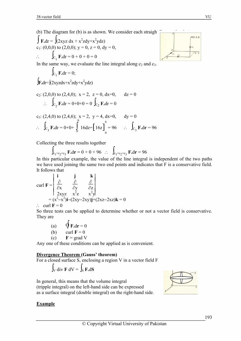
38-vector field VU
(b) The diagram for (b) is as shown. We consider each straight
∫ F.dr = ∫(2xyz dx + x2zdy+x2ydz) z = 0, dy = 0, dz = 0
= 0 In the same way, we evaluate the line integral along c2 and c3.
∫F.dr=∫(2xyzdx+x2zdy+x2ydz)
2: (2,0,0) to (2,4,0); x = 2, z = 0, dx=0, dz = 0
c3: (2,4,0) to (2,4,6); x = 2, y = 4, dx=0, dy = 0
C3 dr = 0+0+ ∫
6
0 16dz=[16z]
6
0 = 96 ∴ ∫C3
F.dr = 96
∫c1+c2+c3 F.dr = 0 + 0 + 96 ∴ ∫c1+c2+c3 F.dr = 96 In this particular example, the value of the line integral is independent of the two paths we have used joining the same two end points and indicates that F is a conservative field. It follows that
curl F =
⎪⎪⎪⎪
⎪⎪⎪⎪
i j k∂∂x
line section in turn.
c1: (0,0,0) to (2,0,0); y = 0,
∴ ∫C1 F.dr = 0 + 0 + 0
∫C1 F.dr = 0;
c
∴ ∫ F.dr = 0+0+0 = 0 ∫ F.dr = 0 C2 C2
∴ ∫ F.
Collecting the three results together
∂
∂y ∂∂z
2xyz x2z x2y
= (x2−x2)i−(2xy−2xy)j+(2xz−2xz)k = 0 ∴ curl F = 0 So three tests can be applied to determine whether or not a vector field is conservative. They are
(a) ∫O F.dr = 0 (b) curl F = 0 (c) F = grad V Any one of these conditions can be applied as is convenient. Divergence Theorem (Gauss’ theorem) For a closed surface S, enclosing a region V in a vector field F
∫V div F dV = ∫S F.dS In general, this means that the volume integral (tripple integral) on the left-hand side can be expressed as a surface integral (double integral) on the right-hand side. Example
© Copyright Virtual University of Pakistan
193

38-vector field VU
Verify the divergence theorem for the vector field F = x2i + zj + yk taken over the region bonded by the planes z = 0, z = 2, x = 0, x = 1, y = 0, y = 3. dV = dx dy dz
we have to show that ∫V div F dV = ∫S F.dS
(a) To find ∫V div F dV
div F = ∇.F = ⎝⎜⎛
⎠⎟⎞∂
∂xi + ∂
∂yj + ∂∂zk . (x2i + zj + yk)
= ∂∂x (x2)+
∂∂y (z)+
∂∂z (y)=2x+0+0=2x
∴ ∫V div F dV=∫V 2x dv=∫∫∫V 2xdzdydx
∫V div F dV = ∫1
0∫
3
0∫
2
02xdzdydx = ∫
1
0∫
3
0 [ 2xz]
2
0 dy dx = ∫
1
0[2xz]
3
0dx = ∫
1
012x dx=[6x2]
1
0 = 6
(b) to find ∫S F.dS i.e. ∫S F.n dS The enclosing surface S consists of six separate plane faces denoted as S1, S2, ….. S6 as shown. We consider each face in turn. F = x2i + zj + yk (i) S1 (base): z = 0; n = − k (outwards and downwards) ∴ F = x2i + yk dS1 = dx dy
∴ ∫S1 F. ndS = ∫∫S1
(x2i+yk).(−k)dydx = ∫1
0∫
3
0(−y) dydx = ∫
1
0 ⎣⎢⎡
⎦⎥⎤−
y2
2
3
0
dx = − 92
(ii) S2 (top): z = 2: n=k dS2=dx dy
∫S2 F.ndS=∫∫S2
(x2i+zj+yk).(k)dydx = ∫1
0∫
3
0y dy dx =
92
(iii) S3 (right-hand end): y = 3; n=j dS3 = dxdzj F = x2i + zj + yk
∴ ∫S F.ndS=∫∫S (x2i+zj+3k).(j)dzdx = ∫ ∫ z dz dx = ∫1
0 ⎣⎢⎡
⎦⎥⎤y2
2
1 2
3 3 0 0
2
0
dx = ∫1
0 2 dx = 2
(iv) S4 (left-hand end): y = 0, n = − j, dS4 = dx dz
∴ ∫S4 F.ndS = − 2
for ∫S4 F.ndS=∫∫S4
(x2i+zj+yk).(−j)dzdx= ∫1
0∫
2
0(− z) dz dx= ∫
1
0 ⎣⎢⎡
⎦⎥⎤−
z2
2
2
0
dx
= ∫1
0 (− 2) dx = − 2
Now for the remaining two sides S5 and S6 . Evaluate these in the same manner, obtaining
∫S5 F.n dS = 6; ∫S5
F.n dS = 0 Check:
© Copyright Virtual University of Pakistan 194
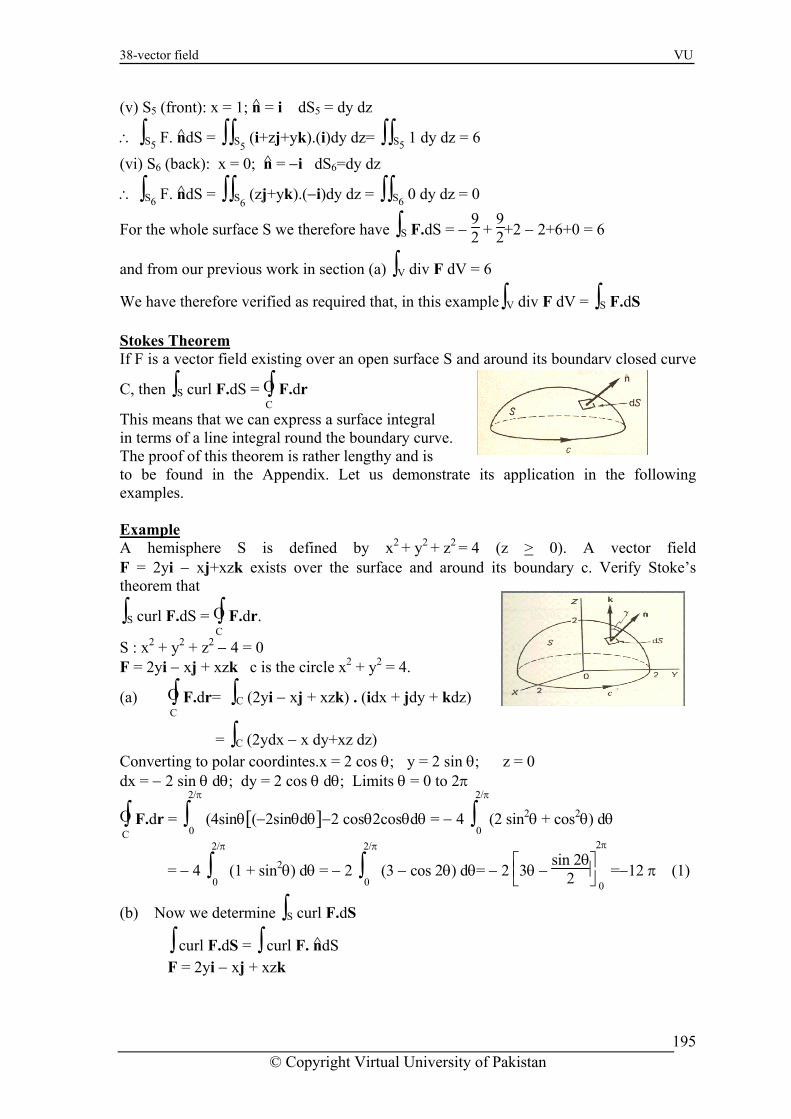
38-vector field VU
(v) S5 (front): x = 1; n = i dS5 = dy dz
∴ ∫S5 F. ndS = ∫∫S5 (i+zj+yk).(i)dy dz= ∫∫S5 1 dy dz = 6
(vi) S6 (back): x = 0; n = −i dS6=dy dz
∴ ∫S6 F. ndS = ∫∫S6 (zj+yk).(−i)dy dz = ∫∫S6 0 dy dz = 0
For the whole surface S we therefore have ∫S F.dS = − 92 +
92+2 − 2+6+0 = 6
and from our previous work in section (a) ∫V div F dV = 6
We have therefore verified as required that, in this example∫V div F dV = ∫S F.dS Stokes Theorem
open surface S and around its boundary closed curve
, then dr
This means that we can express a surface integral
The proof of this theorem is rather lengthy and is to be found in the Appendix. Let us demonstrate its application in the following examples. Example
If F is a vector field existing over an
C ∫S curl F.dS = ∫O F.C
in terms of a line integral round the boundary curve.
A hemisphere S is defined by x2 + y2 + z2 = 4 (z > 0). A vector field
ndary c. Verify Stoke’s theorem that
∫S curl F.dS = ∫OC
F.dr.
S : x2 + y2 + z2 − 4 = 0 F = 2yi − x k c is the circle x2 + y2 = 4.
. + jdy + kdz)
= ∫C (2ydx − x dy+xz dz) Converting to polar coordintes.x = 2 cos θ; y = 2 sin θ; z = 0 x = − 2 sin θ dθ; dy = 2 cos θ dθ; Limits θ = 0 to 2π
F.dr = ∫2/π
0 (4sinθ[(−2sinθdθ]−2 cosθ2cosθdθ = − 4 ∫
2/π
0(2 sin2θ + cos2θ) dθ
= − 4 ∫2/π
0 (1 + sin2θ) dθ = − 2 ∫
2/π
0 (3 − cos 2θ) dθ= − 2 ⎣⎢
⎡⎦⎥⎤3θ −
sin 2θ2
F = 2yi − xj+xzk exists over the surface and around its bou
j + xz
(a) ∫OC
F dr= ∫C (2yi − xj + xzk) . (idx
d
∫OC
2π
0 =−12 π (1)
) Now we determine ∫S curl F.dS
∫ curl F.dS = ∫ curl F. ndS F = 2yi − xj + xzk
(b
© Copyright Virtual University of Pakistan
195

38-vector field VU
curl F =
⎪⎪⎪⎪
⎪⎪⎪⎪
i j k∂∂x
∂∂y
∂∂z
2y −x xz
= i(0−0)−j (z−0)+k (−1−2) = − zj − 3k
ow n= ∇S|∇S|N =
2xi+2yj+2zk4x2+4y2+4z2 =
xi+yj+zk2
hen ∫S curl F. ndS = ∫S (−zk−3k).⎝⎜⎛
⎠⎟⎞xi + yj + zk
2T dS = 12 ∫S (− yz − 3z) dS
x = 2 sinφ cosθ; y = 2 sinφ sinθ; z = 2cos φ , dS = 4 sin φ dφ dθ
∴ ∫S curlF.ndS=12 ∫
S∫(−2 sinφ sinθ 2cosφ− 6 cosφ) 4 sinφ dφ dθ
= − ∫2π
0∫
π/2
0(2sin2 φ cos φ sin θ +3sinφcosφ)dφdθ=−4 ∫
2π
0 ⎣⎢⎡
⎦⎥⎤2 sin3φ sinθ
3 + 3 sin2φ
2
π/2
0 dθ
= − 4∫2π
0 ⎝⎜⎛
⎠⎟⎞2
3 sinθ + 32 dθ = − 12π (2)
So we have from our two results (1) and (2)
∫OC
F.dr
∫S curl F.dS =
© Copyright Virtual University of Pakistan
196

39-Periodic functions VU
Lecture No -39 Periodic Functions
eriodic functions P
function f(x) is said to be periodic if its function values repeat at regular intervals of the independent variable. The regular interval between repetitions is the period of the oscillations. f(x + p) = f(x) Graphs of y = A sin nx
A
ple of a periodic
0° to 360°. π radians and the amplitude, the position of rest.
0° and there are thus 2 complete cycles in 360°.
(a) y = sin x The obvious examfunction is y = sin x, which goes through its complete
x s fromrange of values while increase The period is therefore 360° or 2 the maximum displacement fromy = 5sin 2x The amplitude is 5. The period is 18
Example
Functions Amplitude Period y = 3 sin 5x 3 72° y = 2 cos 3 2 x 120°
y = sin x2 1 720°
y = 4 sin 2 4 x 180° y = A sin nx Thanking along the same lines, th
360°e function y = A sin nx
; period = nhas amplitude = A = 2πn ; n cycles in 360°.
y = A cos nx have the same characteristics Graphs of Example s period = 6 ms period = 5 cm
iodic function
period = 8 m Analytical description of a per
ed analytically in many cases. A periodic function ca
n be defin
Example (a) Between x = 0 and x = 4, y = 3,
) = 0,
4 < x < 6. o we could define the function by
f(x) = 3 0 < x < 4
i.e. f(x) = 3 0 < x < 4nd x = 6, y(b Between x = 4 a
i.e. f(x) = 0S
© Copyright Virtual University of Pakistan
197

39-Periodic functions VU
f (x) = 0 4 < x < 6 (x) = f (x + 6) e last line indicating that the function is periodic
with period 6 units 0 < x < 3
x) = − 1 3 < x < 5
4
f th
f(x) = 2 − x f(f(x) = f(x+5)
f(x) = 3x
0 < x < 4
f(x) = 7 − x 4 < x < 0 =
1f(x) − 3 10 < x < 13 f(x) = f (x + 13) Example Sketch the graphs of the following inserting relevant values. 1. f(x) = 4 0 < x < 5 f(x) = 0 5 < x < 8 f(x) = f (x + 8) f(x) = 3x − x2 0 < x < 3
f(x
f(x) = 0 π < x
f(x) = x4
f(x) = f (x + 3)
) = 2 sin x 0 < x < π < 2π
f(x) = f (x + 2π). 2
0 < x < 4
4 < x < 6 = 0 6 < x < 8
f(x) = f(x + 8).
Useful integrals
f(x) = 4 f(x)
rals appear frequently in our work on Fourier series, so it will help if we obtain the result in readiness. In each case, m and n are integers other than zero.
(a) ∫
π
−πsin nx dx = ⎣⎢
⎡⎦⎥⎤− cos nx
n
The following integ
π
−π =
1n {− cos nπ + cos nπ}= 0
(b) ∫
π
−πcos nx dx = ⎣⎢
⎡⎦⎥⎤sin nx
n
π
−π =
1n {sinnπ + sin nπ} = 0
(c) ∫
π
−π sin2nx dx =
12 ∫
π
−π(1−cos2nx) dx =
12 ⎣⎢
⎡⎦⎥⎤x −
sin 2nx2n
π
−π = π (n ≠ 0)
© Copyright Virtual University of Pakistan
198

39-Periodic functions VU
(d) ∫
π
−πcos2nx dx =
12 ∫
π
−π (1 + cos 2nx) dx =
12 ⎣⎢
⎡⎦⎥⎤x +
sin 2nx2n
π
−π = π (n ≠ 0)
(e) ∫
π
sin nx cos mx dx = 12
−π ∫
π
−π{sin(n+m)x+sin(n−m)x}dx=
12 {0 + 0}= 0
from result (a) with n ≠ m
(f)−π
cos nx cos mx dx = 2 ∫
π
1 ∫−π
{cos(n+m)x+cos(n )x}dx= 2
π
−m1 {0 + 0}= 0
from result (b) with n ≠ m Note:
m, then
∫
π
−π cos nx cos mx dx becomes ∫
π
−πcos2 nx dx = π from (d) above.
(g) ∫
π
−π sin nx sin mx dx = − ½ ∫
π
−π(− 2) sin nx sin mxdx= −½∫
π
−π cos(n+m)x−cos(n−m)xdx
= 2
If n =
π
1 ∫−π
{0 − 0)= 0 from result (b) with n ≠ m
Note: If n = m, then
∫
π
−π sin nx sin mx dx becomes ∫
π
−π sin2 nx dx = π from (c) above
Summary of integrals
(a) ∫
π
−πsin nx dx = 0 , (b) ∫
π
−πcos nx dx = 0 , (c) ∫
π
−πsin2 nx dx = π (≠ 0)
) ∫
π
−πcos2 nx dx = π (n ≠ 0) (e) ∫
π
−πsin nx cos mx dx = 0
) ∫
π
−πcos nx cos mx dx = 0 (n ≠ m) (g) ∫
π
−πsin nx sin mx dx = 0 (n ≠ m)
∫
π
−πcos nx cos mx dx = π (n = m) ∫
π
−πsin nx sin mx dx = π (n = m)
Note
(d
(f
e have evaluated the integrals between − π and π, but, provided integration is carried ut over a complete periodic interval of 2π, the results are the same. Thus, the limits ould just as well be − π to π, 0 to 2π, − π/2 to 3π/2, etc. We can therefore choose the mits to suit the particular problems.
Wocli
© Copyright Virtual University of Pakistan
199

39-Periodic functions VU
Fourier series eriodic functions of period 2πP he basis of a Fourier series is to represent a periodic function by a trigonometrical series f the form. x) = A0+c1 sin (x+α1) + c2 sin (2x+α2) +c3 sin (3x+α3)+…+cn sin (nx+αn)+ … here A0 is a constant term
1, c2, c3….cn denote the amplitudes of the compound sine terms α1, α2, α3….. are onstant auxiliary angles. ach sine term, cn sin (nx + αn) can be expanded thus: n sin (nx + αn) = cn{sin nx cosαn+cos n x sinαn}= (cnsinαn) cos nx + (cncosαn) sin nx
ncos nx + bnsin nx e whole series becomes.
f(x) = A0 + ∞
∑ n=1
{an cos nx + bn sin nx}
Tof(wccEc= ath
© Copyright Virtual University of Pakistan
200

40-Fourier series VU
Lecture No- 40 Fourier Series
As we know that A0 + ∞
∑ n=1
{ancosnx + bnsinnx};
which can be written as in the expanded from A0+(a1cosx+b1sinx)+(a2cos2x+b2sin2x)+ .... + (ancos nx+bnsin nx)+........... A0+a1cosx+a2cos2x+.+ancos nx+.. .. +b1sinx+b2sin2x+... bnsin nx+.......... f(x) = A0+a1cosx+a2cos2x+.+ancos nx+.. ....+b1sinx+b2sin2x+... bnsin nx+... Fourier coefficients We have defined Fourier series in the form
f(x) =A0 + ∞
∑ n=1
{ancosnx + bnsinnx}; n a positive integer
(a) To find A0, we integrate f(x) with respect to x from − π to π.
∫
π
−πf(x)dx = ∫
π
−πA0 dx +
∞
∑ n=1
⎩⎪⎨⎪⎧
⎭⎪⎬⎪⎫
∫
π
−πan cos nx dx+∫
π
−πbn sin nx dx = [A0x]
π
−π +
∞
∑ n=1
{ 0 + 0 } = 2A0π
2A0 π = ∫
π
−π f(x) dx
A0 = 1
2π ∫
π
−π f(x) dx =1/2 a0 ; Where a0 =
1π ∫
π
−π f(x) dx
(b) To find an we multiply f(x) by cos mx and integrate from − π to π.
∫
π
−πf(x)cos mx dx = ∫
π
−πA0 cos mx dx+
∞
∑ n=1
⎩⎨⎧
⎭⎬⎫
∫
π
−π
an cos nx cos mx dx+∫
π
−π
bn sin nx cos mx dx
∫
π
−πf(x)cos mx dx = A0 {0} +
∞
∑ n=1
{an (0) + bn (0)}= 0 for n ≠ m
0 + a= nπ + 0 = anπ for n = m π
∴ an = 1π ∫
−π
(c) To find b
f(x) cos nx dx
multiply f(x) by sinmx and integrate from − π to π.
−π +∑
n=1 ⎩⎨
⎭⎬⎫
∫−π
an cosnxsinmx dx+∫
π
−π
bn sin nx sinmxdx
−π A0 {
n we
∫ f(x)sin mx dx = ∫ A
π π∞ ⎧
π
−ππ
∞
0 sin mx dx
∫ f(x)sin mx dx = 0} + ∑ ) + bn (0)}= 0 for n ≠ m
= 0 + 0 + bnπ = bnπ for n = m
∴ bn = 1π
n=1
{an (0
∫
π
−π f(x) sin nx dx
© Copyright Virtual University of Pakistan
201

40-Fourier series VU
Result For Fourier Series
f(x)=12 a0+
∞
∑ n=1
{ancosnx+bnsinnx};
(a) a0 = 1π ∫
π
−π f(x) dx = 2×mean value of f(x) over a period
(b) an = 1π ∫
π
−π f(x) cos nx dx=2×mean value of f(x) cosnx over a period.
(c) bn = 1π ∫
π
−π f(x) sin nx dx = 2 × mean value of f(x) sin nx over a period.
In each case, n = 1, 2, 3, …… Example Determine the Fourier series to represent the periodic function shown. It is more convenient here to take the limits as 0 to 2π. The function can be defined as
f(x) = x2 0 < x < 2π
f(x) = f(x + 2π) period = 2π. Now to find the coefficients
(a) a0 = 1π ∫
2π
0 f(x) dx=
1π ∫
2π
0 ⎝⎜⎛
⎠⎟⎞x
2 dx = 1
4π [x2]2π
0 = π
a = π
(b) an = 1π
02π
∫0
f(x) cos nx dx
= 1π ∫
2π
0 ⎝⎜⎛
⎠⎟⎞x
2 cos nx dx
a = 1
n 2π ∫0
x cos nx dx = 2π
2π
1 ⎩⎪ n⎨⎪⎧
⎭⎪⎬⎪⎫[x sin nx]
2π
− 1n
0 ∫
2π
0sin nx dx =
12π
⎩⎪⎨⎪⎧
⎭⎪⎬⎪⎫
(0 − 0) − 1n (0)
a = 0 ∴ n
(a) bn = 1π ∫ f(x) sin nx dx So
2π
0e w now have
bn = 1π ∫
0
x2
2π
sin nx dx= 1
2π ⎩⎪⎨
⎭⎪⎬⎪⎫[−
x cosnxn
⎪⎧ ]2π
0 +
1n ∫
2π
0cos nx dx = −
12πn [2π − 0]= −
1n
0 = π n = 0 1n a ; a ; bn = −
Now the general expression for a Fourier series is
f(x) = 12 a0 +
∞
∑ n=1
{an cos nx + bn sin nx} Therefore in this case
© Copyright Virtual University of Pakistan
202

40-Fourier series VU
f(x) = π2 +
∞
∑ n=1
{bn sin nx} = π2 +{−
11 sinx−
12 sin2x−
13 sin3x−...} since an = 0
f(x) = π2 −{sinx+
12 sin2x+
13 sin3x+.......}
Dirichlet Conditions If the Fourier series is to represent a function f(x), then putting x = x1 will give an infinite series in x1 and the value of this should converge to the value of f(x1) as more and more terms of the series are evaluated. For this to happen, the following conditions must be fulfilled. (a) The function f(x) must be defined and single-valued. (b) f(x) must be continuous or have a finite number of finite discontinuities within a periodic interval. (c) f(x) and f
′(x) must be piecewise continuous in the periodic interval.
If these Dirichlet conditions are satisfied, the Fourier series converges to f(x1), if x = x1 is a point of continuity Example Find the Fourier series for the function shown. Consider one cycle between x=0 and x=π. The function can be defined by
0 − π < x < − π2 f(x) =
f(x) = 4 − π2 < x <
π2
f(x) = 0 π2 < x < π
f(x) = f (x + 2π)
f(x) = 12 a0 +
∞
∑ n=1
{an cos nx+bn sin nx}
a0 = 1
is πThe expression for a0 ∫
π
(x) dx is gives
a0 = 1π
−π f Th
⎩⎪⎨
⎭⎪⎬⎪
∫−π
0 dx + ∫ −π/2
4dx + ∫π/2
0 dx = 1π
⎪⎧ ⎫−π/2 π/2 π
[4x]π/2
−π/2=4
a0 = 4
(b) an = 1π ∫
π
−π f(x) cos nx dx =1
π ⎩⎨⎧
⎭⎬⎫
∫
−π/2
−π
(0)cosnxdx+∫
π/2
−π/2
4cosnxdx+ ∫
π
π/2
(0) cosnxdx = 1π
⎩⎪⎨⎪⎧
⎪⎬⎪⎫
∫
π/2
−π/2 4cosnxdx
⎭
= 4
πn sin nx | π/2
−=
8π/2 πn sin
nπ2
an = πn8
sin n2π
Then considering different integer values of n, we have If n is even an = 0
an = 8
nπ If n = 1.5, 9….
© Copyright Virtual University of Pakistan
203

40-Fourier series VU
If n = 3, 7, 11, …. an = − 8
nπ
(c) To find bn
bn = 1π ∫
π
−πf(x) sin nx dx =
1π
⎩⎨⎧
⎭⎬⎫
∫
−π/2
−π
(0)sinnxdx+∫
π/2
−π/2
4sinnxdx+ ∫
π
π/2
(0) sinnxdx
bn = 4π ∫
π/2
−π/2sin nx dx =
4π ⎣⎢
⎡⎦⎥⎤− cos nx
n
π/2
−π/2 = −
4nπ
⎩⎪⎨⎪⎧
⎭⎪⎬⎪⎫
cos nπ2 − cos ⎝⎜
⎛⎠⎟⎞− nπ
2 = 0
bn = 0
o with a0 = 4: an as stated above; bn = 0;
f(x) = 2 + 8π
S The Fourier series is
{cosx − 13 cos 3x +
15 cos5x −
17 cos 7x + …..}
In this particular example, there are, in fact, no sine terms. Effect Of Harmonics It is interesting to see just how accurately the Fourier series represents the function with which it is associated. The complete representation requires an infinite number of terms, but we can, at least, see the effect of including the first few terms of the series. Let us consider the waveform shown. We established earlier that the function
f(x) = 0 π < x < − π
− 2
f(x) = 4 − 2π
< x < 2π
f(x) = 0 π2 < x < π
f(x) = f (x + 2π) gives the Fourier series
8f(x) = 2 + π {cos x−3
1 cos3x + 3
1 cos 5x − 7
1 cos 7x + ….}
If we start with just one cosine term, we can then see the effect o including subsequent harmonics. Let us restrict our attention to just the right-hand half of the symmetrical waveform. Detailed plotting of points gives the following development.
) f(x) = 2 + 8π
cos x (1
© Copyright Virtual University of Pakistan
204

40-Fourier series VU
(2) f(x) = 2 + 8π {cosx −
13 cos 3x}
(3) f(x)=2+
8π {cos x−
13 cos3x +
13 cos5x)
(4) f(x) = 2 + π
8 {cosx−
13 cos3x+
13 cos5x −
17 cos 7x}
As the number of terms is increased, the graph gradually approaches the shape of the original square waveform. The ripples increase in number and decrease in amplitude, but a perfectly square wave rm is unattainable in practice. For practical purpose, the first few terms l su ce to give an accuracy of acc
fonormal y ffi eptable level.
© Copyright Virtual University of Pakistan
205

41-Examples VU
Lecture No -41 Examples Example Find the Fourier series for the function defined by f(x) = x − π x < 0
The general expressions for a0 n n
− <f(x) = 0 0 < x < π f(x) = f (x + 2π)
, a , b are
a0 = 1π ∫ f(x) dx , a
π
n = 1π ∫ f(x) cos nx dx , b
π
−πn =
1π ∫
π
−π f(x) sin nx dx
−π
a0 = 1π ∫
−π f(x) dx =
1π
π
∫
0
−π(− x) dx +
1π ∫
00 dx =
1π
π
∫
0
−π(− x) dx =
1π ⎣⎢
⎡⎦⎥⎤−
x2
2
0
−π =
π2
(b) To find an
∫
π
f(x) cos nx dx = 1π ∫
0
−π(−x) cosnxdx +
1π ∫
π
00 dx = −
1π ∫
π
−πx cos nx dx an = π
1 −π
= − 1π ⎨
⎪[x
sin nxn⎩⎪ ⎭⎪
⎬⎪⎫⎧
] 1n
0
−π − ∫ s
0
−πin nx dx = −
1π
⎩⎪⎨⎪⎧
⎭⎪⎬⎪⎫
(0 − 0) − 1n⎣⎢⎡
⎦⎥⎤− cos nx
n
0
−π
1= − π
⎩⎪⎨
⎭⎪⎬n
⎪⎧ ⎪⎫1⎣⎢ ⎦⎥n⎡ ⎤ cos nx 0 1
−π = − πn2
⎩⎪⎨⎣⎢ n
⎪⎧
⎭⎪⎬⎪⎫⎡
⎦⎥⎤ cos nx 0
−π = −
1πn2 [cos 0 − cos nπ]
1= − πn2 {1 − cos nπ}
But cos nπ = 1 (n even) and cos nπ = − 1 (n odd)
an = − 2
πn2 (n odd) and an = 0 (n even)
(c) Now to find bn
bn = 1π ∫
π
−π f(x)sinnxdx =
1π ∫
0
−π(−x) sin nx dx = −
1π ∫
0
−πx sin nx dx
= −1π
⎩⎪⎨⎪⎧
⎭⎪⎬⎪⎫
[x ⎝⎜⎛
⎠⎟⎞−cos nx
n ]0
−π +
1n ∫
0
−πcos nx dx =−
1π
⎩⎪⎨⎪⎧
⎭⎪⎬⎪⎫πcosnπ
n +1n ⎣⎢
⎡⎦⎥⎤sin nx
n 0
−π =
cos nπn
bn = 1n (n even) and bn= -
1n (n odd)
So we have
a0 = π2 ; an = 0 (n even) and an = −
2πn2 (n odd)
bn = − n1
(n even) and bn = 1n (n odd)
f(x)=π4 −
2π ⎝⎜
⎛⎠⎟⎞cosx+
19 cos3x+
125 cos 5x+... + ⎝⎜
⎛⎠⎟⎞sin x −
12 sin 2x +
13 sin 3x −
14 sin 4x+….
It is just a case of substituting n = 1, 2, 3, etc. In this particular example, we have a constant term and both sine and cosine terms.
© Copyright Virtual University of Pakistan
206
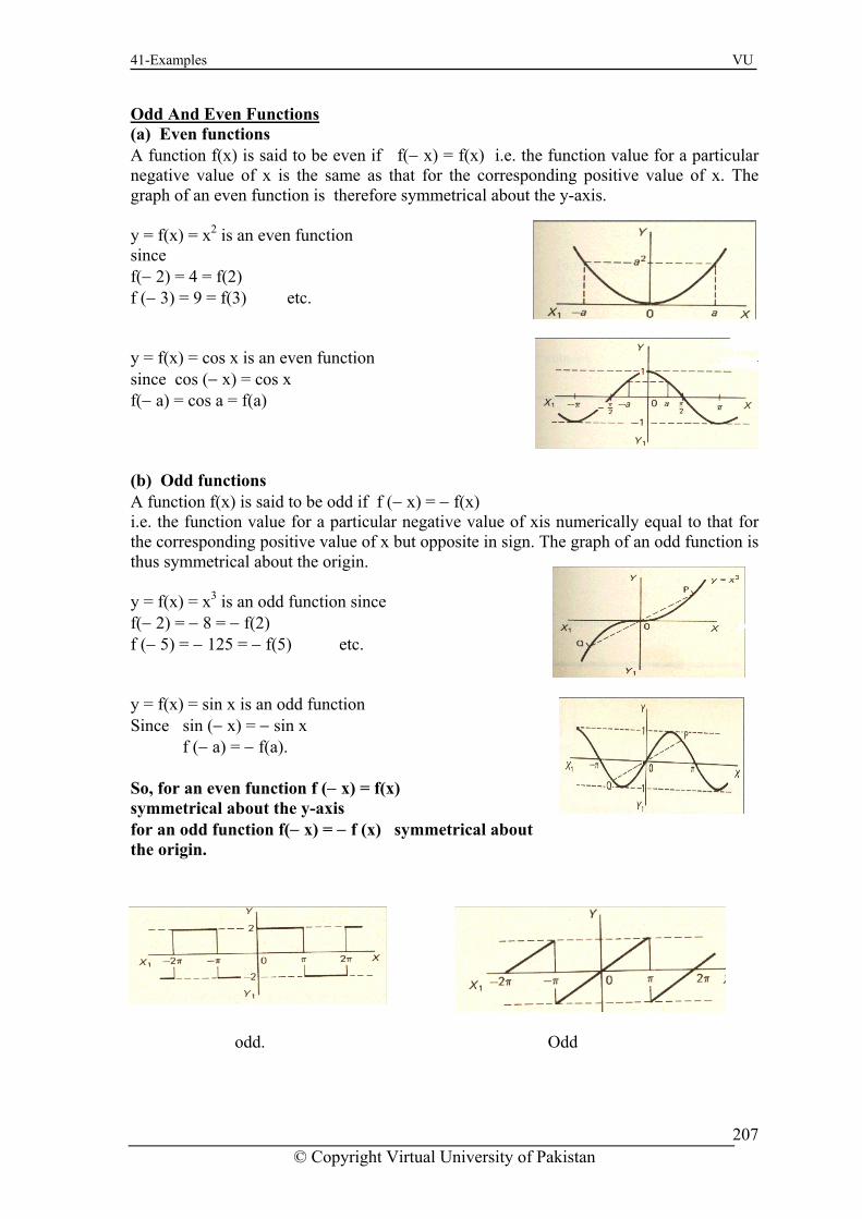
41-Examples VU
Odd And Even Functions (a) Even functions A function f(x) is said to be even if f(− x) = f(x) i.e. the function value for a particular negative value of x is the same as that for the corresponding positive value of x. The graph of an even function is therefore symmetrical about the y-axis. y = f(x) = x2 is an even function since f(− 2) = 4 = f(2) f (− 3) = 9 = f(3) etc. y = f(x) = cos x is an even function since cos (− x) = cos x f(− a) = cos a = f(a) (b) Odd functions A function f(x) is said to be odd if f (− x) = − f(x) i.e. the function value for a particular negative value of xis numerically equal to that for the corresponding positive value of x but opposite in sign. The graph of an odd function is thus symmetrical about the origin. y = f(x) = x3 is an odd function since f(− 2) = − 8 = − f(2) f (− 5) = − 125 = − f(5) etc. y = f(x) = sin x is an odd function
r an odd function f(− x) = − f (x) symmetrical about
Since sin (− x) = − sin x f (− a) = − f(a). So, for an even function f (− x) = f(x) symmetrical about the y-axis fothe origin.
odd. Odd
© Copyright Virtual University of Pakistan
207

41-Examples VU
Odd
Products Of Odd And Even Functions
Even neither
Even
The rules closely resemble the elementary rules of signs. (even)×(even)=(even) like (+)×(+)=(+) ; (odd)× (odd) = (even) (−)×(−)=(+) ; (odd)× (even) = (odd) (−)×(+)=(−)
) Two even functions and g(x) are even functions.
(− x) = f(x) g(x) since f(x) and g(x) are even. F(− x) = F(x)
F(x) is even
e f(x) and g(x) are odd functions. en F(− x) = f(− x) g(− x) = {− f (x)} {− g(x)}
(x) are odd. (x) = F (x)
F(− x) = F(x) F (x) is even Finally (c) One odd and one even function Let F(x) = f(x) g(x) where f(x) is odd and g(x) even. Then F (− x) = f (− x) g(− x) = − f(x) g(x) = − F (x) ∴ F (− x) = − F (x) F (x) is odd So if f(x) and g(x) are both even, then f(x) g(x) is even and if f(x) and g(x) are both odd, then f(x) g(x) is even but if either f(x) or g(x) is even and the other odd. Then f(x) g(x) is odd.
The results can easily be proved. (aLet F(x) = f(x) g(x) where f(x)Then F(− x) = f(− x) g∴ (b) Two odd functions
et F(x) = f(x) g(x) wherLThsince f(x) and g = f(x) g∴
© Copyright Virtual University of Pakistan
208

41-Examples VU
Example State whether each of the following products is odd, even, or neither. 1. x2 sin 2x odd (E) (O) = (O) 2. x3 cos x odd (O) (E) = (O) 3. cos 2x cos 3x even (E) (E) = (E) 4. x sin nx even (O) (O) = (E) 5. 3 sin x cos 4x odd (O) (E) = (O) 6. (2x + 3) sin 4x neither (N) (O) = (N) 7. sin2 x cos 3 x even (E) (E) = (E)
9. (x + 4) sin 2x odd (E) (O) = (O)
8. x3ex neither (O) (N) = (N) 4
Two useful facts emerge from odd and even functions. (a) For an even function
∫
a
−a f(x)dx=2∫
a
0 f(x) dx
(b) For an odd function
∫
a
−a f (x) dx = 0
THEOREM 1 If f(x) is defined over the interval − π < x < π and f(x) is even, then the Fourier series for f(x) contains cosine terms only. Included in this is a0 which maybe regarded as an cos nx with n = 0. Proof:
(a) a0 = 1π ∫
π
−π f(x)dx =
2π ∫
π
0 f(x)dx ∴ a0 =
2π ∫
π
0 f(x) dx
(b) an = 1π ∫
π
−π f(x) cos nx dx.
But f(x) cos nx is the product of two even functions and therefore itself even.
an = 1π ∫
π
−π f(x) cos nx dx =
2π ∫
π
0 f(x) cos nx dx. ∴ an =
2π ∫
π
0 f(x) cos nx dx
(c) bn = 1π ∫
π
−π f(x) sin nx dx
Since f(x) sin nx is the product of an even function and an odd function, it is itself odd.
∴ bn = 1π ∫
π
−π f(x) sin nx dx = 0.
∴ bn = 0 Therefore, there are no sine terms in the Fourier series for f(x).
© Copyright Virtual University of Pakistan
209

41-Examples VU
Example The waveform shown is symmetrical about the y-axis. The function is therefore even and there will be no sine terms in the series.
∴ f(x) = 12 a0 +
∞
∑ n=1
an cos nx
(a) a0 = 1π ∫
π
−π f(x) dx =
2π ∫
π
0 f(x) dx.=
2π ∫
π/2
0 4 dx
= 2π [4x]
π/2
0 = 4
(b) an = 1π ∫
π
−π f(x)cos nx dx =
2π ∫
π
0 f(x) cos nx dx=
2π ∫
π/2
0 4cosnx dx=
8π ⎣⎢
⎡⎦⎥⎤sin nx
n
π/2
0
= 8
πn sin nπ2
But sin nπ2 = 0 for n even
= 1 for n 1, 5, 9, ….. = − 1 for n = 3, 7, 11, …. an = 0 (n even);
an = 8
πn (n = 1, 5, 9, ….);
a = − 8
n πn (n = 3, 7, 11 ……)
sinc ven function.Therefore, the required series is
π
(c) bn = 0, e f(x) is an e
f(x) = 2 + 8 {cos x − 13 cos 3x +
13 cos 5x −
17 cos 7x + ….}
Theorem 2: If f(x) is an odd function defined over the interval − π < x < π, then the Fourier series for f(x) contains sine terms only. Proof: Since f(x) is an odd function
∫
0
−π f(x) dx = − ∫
π
0 f(x) dx.
(a) a0 = 1π ∫
π
−π f(x) dx.
But f(x) is odd ∴ a0 = 0
(b) an = 1π ∫
π
−π f(x) cos nx dx
Remembering that f(x) is odd and cosnx is even, the product f(x) cosnx is odd.
∴ an = 1π ∫
π
f(x) cosnx dx = 1
−π π ∫π
(odd function) dx
n
−π
∴ a = 0
© Copyright Virtual University of Pakistan
210

41-Examples VU
(b) bn = 1π ∫
π
−π f(x) sin nx dx
and since f(x) and sin nx are each odd, the product f(x) sin nx is even.
hen bn = 1π ∫
π
−π (even function) dx =
2π ∫
π
0 f(x) sin nx dx
bn = 2π
T
∴ ∫π
0 f(x) sin nx dx
o, f(x) is odd function then a0 = 0; an = 0;
bn = 2π
SIf
∫π
0 f(x) sin nx dx i.e. th s only.
Example
e Fourier series contains sine term
− π < x < 0
f(x) = 6 0 < x < π f(x) = f(x + 2π)
We can see that this is an odd function; a0 = 0 and an = 0
bn = 1π
f(x) = − 6
∫π
−π f(x) sin nx dx.
f(x) sin nx is a product of two odd functions and is therefore even.
∴ bn = 2π ∫
π
0 f(x) sin nx dx
bn = 2π ∫
π
6 sin nx dx = 12π ⎣⎢
⎡⎦⎥⎤− cos nx
n
π
= 12
0π ⎣⎢
⎡⎦⎥⎤cos nx
n
0
π
= 12π [cos 0 − cos nπ]
0
= 12πn (1 − cos nπ).
bn = 0 (n even) bn = 24πn (n odd)
So the series is f(x) = 24π {sinx +
13 sin3x +
15 sin5x +….}
Of course, if f(x) is neither an odd nor an even function, then we must obtain expressions for a0, an and bn in full.
© Copyright Virtual University of Pakistan
211

42-Examples VU
Lecture No -42 Examples Example Determine the Fourier series for the function shown.
en. 0, an and bn.
This is neither odd nor evherefore we must find aT
f(x) = 12 a0 + ∑
n = 1 {a
∞
f(x) = π
n cos nx + bn sin nx}
2 x 0 < x < π
= 2 , π < x < 2π
(a) a0 = 1π ∫
2π
0 f(x)dx =
1π
⎩⎨⎧
⎭⎬⎫
∫π
0 2π x dx + ∫
2π
π 2 dx =
1π
⎩⎨⎧
⎭⎬⎫
⎣⎢⎡
⎦⎥⎤x2
π
π
0+ [2x]
2π
π =
1π {π + 4π − 2π}
∴ a0 = 3
(b) an = 1π ∫
2π
0 f(x) cos nx dx =
1π ⎩
⎨⎧
⎭⎬⎫
∫
π
0 ⎝⎛
⎠⎞2
πx cos nx dx + ∫
2π
π 2 cos nx dx
= 1π ⎩
⎨⎧
⎭⎬⎫2
π ∫
π
0 x cosnx dx + 2∫
2π
π cosnxdx =
2π ⎩
⎨⎧
⎭⎬⎫1
π ∫
π
0 x cosnx dx + 2∫
2π
π cosnxdx
=2π
⎣⎢⎡
⎦⎥⎤
⎩⎨⎧
⎭⎬⎫1
π⎣⎡ ⎦⎤x sin nx
n
π
0
− 1
πn ∫2π
0 sinnxdx +∫
2π
π cosnxdx =
2π
⎩⎨⎧
⎭⎬⎫
0 − 1
nπ ⎣⎢⎡
⎦⎥⎤−
cos nxn
π
0 + ⎣⎢
⎡⎦⎥⎤sin nx
n
2π
π
= 2π
⎩⎨⎧
⎭⎬⎫1
nπ ⎣⎢⎡
⎦⎥⎤cos nx
n
π
0 =
2π2n2 {cos nπ − cos 0}=
2π2n2 {cos nπ − 1}
an= 0 (n even); an= − 4π2n2 (n odd)
(c) To find bn, we proceed in the same general manner
bn = 1π ∫
2π
0 f(x) sin nx dx=
1π ⎩
⎨⎧
⎭⎬⎫
∫
π
0 ⎝⎛
⎠⎞2
πx sin nx dx + ∫
2π
π 2 sin nx dx
= 2π
⎩⎨⎧
⎭⎬⎫1
π ⎣⎡ ⎦⎤−x cos nx
n
π
0
+1
πn ∫
π
0 cosnxdx+∫
2π
π sinnxdx =
2π
⎩⎪⎨⎪⎧
⎭⎪⎬⎪⎫1
πn (−π cosnπ)+1
πn⎣⎡
⎦⎤sin nx
n
π
0
+⎣⎡
⎦⎤− cos nx
n
2π
π
= 2π
⎩⎨⎧
⎭⎬⎫
−1n cosnπ+(0−0)−
1n (cos 2πn−cosnπ) =
2π
⎩⎨⎧
⎭⎬⎫
−1n cosnπ+(0−0)−
1n cos 2πn+
1n cosnπ
= 2π
⎩⎪⎨⎪⎧
⎭⎪⎬⎪⎫
− 1n cos 2nπ = −
2πn cos 2nπ
But cos 2nπ = 1.
2
πn∴ bn = −
So the required series is
f(x) =32 −
4π2
⎩⎪⎨⎪⎧
⎭⎪⎬⎪⎫
cosx+19cos3x+
125cos5x+… −
2π
⎩⎪⎨⎪⎧
⎭⎪⎬⎪⎫
sinx+12sin2x+
13sin3x+
14 sin4x…
Sum of a Fourier series at a point of discontinuity
© Copyright Virtual University of Pakistan
212
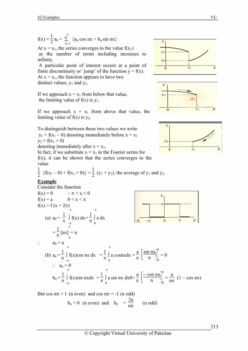
42-Examples VU
f(x) = 12 a0 +
∞
∑ n=1
{an cos nx + bn sin nx}
At x = x1, the series converges to the value f(x1) as the number of terms including increases to infinity. A particular point of interest occurs at a point of
ity or `jump’ of the function y = f(x). At x = x1, the function appears to have two distinct values, y1 and y2. If we approach x = x1 from below that value, the limiting value of f(x) is y1. If we approach x = x1 from above that value, the
te 1
urier series for nverges to the
value 1
finite discontinu
limiting value of f(x) is y2. To distinguish between these two values we wri y1 = f(x1 − 0) denoting immediately before x = xy = f(x + 0) 2 1denoting immediately after x = x . 1In fact, if we substitute x = x1 in the Fof(x), it can be shown that the series co
0)} = 12 (y1 + y2), the average of y1 and y2. 2 {f(x1 − 0) + f(x1 +
Example Consider the function f(x) = 0 − π < x < 0 f(x) = a 0 < x < π f(x) = f (x + 2π)
(a) a0 = 1π ∫ f(x) dx=
1π
π
−π ∫ a dx
π
0
= 1π [ax]
π
0= a
∴ a0 = a
(b) an = 1π ∫
π
−πf(x)cos nx dx =
1π ∫
π
0a cosnxdx =
aπ ⎣⎢
⎡⎦⎥⎤sin nx
n
π
0 = 0
bn = π
∴ an = 0
1 ∫−π
f(x)sin nxdx = π
π
1 ∫
0a sin nx dx0= π
π
a ⎣⎢ ⎦⎥
⎤− cos nxn
⎡π
0 =
anπ (1 − cos nπ)
os nπ = -1 (n odd)
= 0 (n even) and bn = 2a
But cos nπ = 1 (n even) and c
bn nπ (n odd)
© Copyright Virtual University of Pakistan
213

42-Examples VU
f (x) = 21 a0 + ∑ b
∞
n sin nxn=1
af(x) = 2 + π
2a {sinx + 3
1 sin3x + 5
1 sin5x +....}
A finite discontinuity, or `jump’, occurs at x = 0. If we substitute x = 0 in the series
f(x) = a/2, which is, in fact, the average of the two function values at x = 0. Note also that at x = π, another finite discontinuity occurs and substituting x = π in the series gives the same result. Because of this ambiguity, the function is said to be `undefined’ at x = 0, x = π, etc. Half-Range Series
obtained, all the sine terms vanish and we get
Sometime a function of period 2π is defined over the range 0 to π, instead of the normal − π to π, or 0 to 2π. We then have a choice of how to proceed.
x = 0 and x = π, f(x) = 2x, then, since the period is 2π, we have no evidence of how the function behave between x = − π and x = 0. If the waveform were as shown in (a), the function would be an even function, symmetrical about the y-axis and the series would have only cosine terms (including possibly a0).
tio e odd, being symmetrical and the series would have only sine terms.
Example
For example, if we are told between
On the other hand, if the waveform were as shown in (b), the func n would babout the origin
n. To obtain a cosine series, i.e. a series with no sine terms, we need an even function. Therefore, we assume the waveform between x = − π and x = 0 to be as shown, making the total graph symmetrical about the y-axis. Now we can find expressions for the Fourier coefficients as usual.
a0 = 2π
A function f(x) is defined by f(x) = 2x 0 < x < π f(x) = f(x + 2π) Obtain a half-range cosine series to represents the functio
∫π
0 f(x)dx =
2π ∫
π
0 2xdx =
2π [x2]
π
0 = 2π
∴ a0 = 2π
© Copyright Virtual University of Pakistan
214

42-Examples VU
an = 1π ∫
π
−π f(x) cos nx dx =
2π ∫
π
0 f(x) cos nx dx
an = 2π ∫
π
0 2x cos nx dx =
4π ∫
π
0 x cos nx dx =
4π
⎩⎪⎨⎪⎧
⎭⎪⎬⎪⎫
⎣⎢⎡
⎦⎥⎤x sin nx
n
π
0 −
1n ∫
π
0 sin nx dx
= 4π
⎩⎪⎨⎪⎧
⎭⎪⎬⎪⎫
(0−0) − 1n ⎣
⎡⎦⎤− cos nx
n
π
0
= (4
πn2) (cos nπ− 1)
cos nπ = 1 (n even) and cos nπ = −1 (n odd)
∴ a = 0 (n even) and an = − 8
πn2 (n odd)
d an = −8
πn
n
All that now remains is bn which is zero, since f(x) is an even function, i.e. bn = 0
So a0 = 2π, an = 0 (n even) an 2 (n odd),
bn = 0. Therefore
f(x)=π−8π
⎩⎪⎨
⎭⎪⎬⎪⎫
cosx+19
⎪⎧ cos3x+
125 cos5x+….
xample EDetermine a half-range sine series to repressent the function f(x) defined by
x) = 1 + x 0 < x < π f(x) = f(x + 2π)
e choose the waveform between = − π and x = 0 so that the graph is symmetrical out the origin. The function is then an odd
function and the series will contain only sine terms.
∴ a0 = 0 and an = 0
n = 1π
f(
Wx
ab
b ∫π
−π f(x) sin nx dx
n = 2πb ∫
π
0 f(x) sin nx dx
n = 2πb ∫
π
0 (1+x)sin nx dx =
2π
⎩⎪⎨⎪⎧
⎭⎪⎬⎪⎫
⎣⎢⎡
⎦⎥⎤(1 + x)
− cosnxn
π
0 +
1n ∫
π
0 cosnxdx
= 2π
⎩⎨⎧
⎭⎬⎫
− 1 + π
n cos nπ + 1n+
1n ⎣⎢
⎡⎦⎥⎤sin nx
n
π
0 =
2π
⎩⎪⎨⎪⎧
⎭⎪⎬⎪⎫1
n − 1 + π
n cos nπ = 2
πn {1 − (1 + π) cos nπ}
nπ = 1 (n even) and cos nπ = − 1 (n odd)
∴ bn= − 2n
cos
(n even)
∴ = 4+2π
πn (n odd)
ubstituting in the general expression f(x) = ∞
∑x = 1
bn sin nx we have S
© Copyright Virtual University of Pakistan
215

42-Examples VU
x)=4 + 2π
π {sinx +13 sin3x+
15 sin5x+...}− 2 {
12 sin 2x+
14 sin 4x+
16 sin 6x+ ....)
d the required series obtained
x)=⎝⎜⎛
⎠⎟⎞4
π
f(
an
f( +2 {sin x+13 sin 3x+
15 sin 5x+..}− 2{
12 sin 2x+
14 sin 4x+
16 sin 6x+ .....}
o knowledge of odd and even functions and of half-range series saves a deal of nnecessary work on occasions.
Su
© Copyright Virtual University of Pakistan
216

43-Functions with periods other than 2π VU
Lecture No.-43 Functions With Periods Other Than 2π So far, we have considered functions f(x) with period 2π. In practice, we often encounter
functions defined over periodic intervals other than 2π, e.g. from 0 to T, − T2 to
T2 etc.
Functions With Period T
If y = f(x) is defined in the range − T2 to
T2 , i.e. has a period T, we can convert this to an
π by changing the units of the independent variable.
terva oted b
s and the the
periodic function is therefore given by f = 1T
interval of 2In many practical cases involving physical oscillations, he ind le is d the periodic t ependent variab time (t) an
ally dein l is norm n y T, i.e. f(t) = f(t + T) Each cycle is therefore completed in T second frequency f hertz (oscillations per second) of
. If the
angular velocity, ω radians per seconds, is defined by ω = 2πf, then
ω = 2πT and T =
2πω
The angle, x radians, at any time t is therefore x = ωt and the Fourier series to represent the function can be expressed as
f(t) = 12 a0 +
∞∑x=1
{anCos nωt +bnSin nωt}
which can also be written in the form
f(t) = 12 A0+
∞∑x=1
Bn sin (nωt + φn) n = 1, 2, 3, .....
Fourier Coefficients With the new variable, the Fourier coefficients become:
f(t) = 12 a0 +
∞∑x=1
{an cosnωt + bn sinnωt}
a0 = 2T ∫
T
0f(t) dt =
ωπ ∫
2π/ω
0f(t) dt
an = 2T ∫
T
0f(t) cos nωt dt =
ωπ ∫
2π/ω
0f(t)cos nωt dt
bn = 2T ∫
T
0f(t) sin nωt dt=
ωπ ∫
2π/ω
0f(t)sin nωt dt
We can see that there is very little difference between these expressions and those that
have gone before. The limits can, of course, be 0 to T, − T2 to
T2 , −
πω to
πω , 0 to
2πω etc.
Example
as is convenient, so long as they cover a complete period.
Determine the Fourier series for a periodic function defined by
© Copyright Virtual University of Pakistan
217

43-Functions with periods other than 2π VU
f(t) = 2 (1 + t) − 1 < t < 0 f(t) = 0 0 < t < 1
f(t) =
12
f(t) = f (t + 2) The first step is to sketch the wave which is.
a0+∞∑x=1
{an cos nωt+bn sin nωt})
T = 2
2a0 = T ∫ f(t) dt = 2
T/22
−T/2∫
1
f(t) dt = ∫0
2 (1 + t) dt + ∫1
(0) dt= [2t + t2]0
= 1
T
−1 −1 0 1
∴ a = 1 0
an = 2
∫ f(t)cosnωtdt2
T/2
−T =
/2 2 ∫ f(1
−1t)cosnωt dt= ∫
0
−1 2 (1 + t) cosnωt dt
⎩ ⎭⎪⎬⎪⎫
⎦⎥⎤sin n
nωan=2 ⎪⎨⎣⎢⎡(1+t)
⎪⎧ ωt0
−1 −
1nω∫
0
−1sinnωtdt = 2
⎩⎨⎧
⎭⎬⎫
(0−0) − 1
nω ⎣⎢⎡
⎦⎥⎤−
cos nωtnω
0
−1
= 2
n2ω2 (1 − cos nω)
Now T = 2πω
∴ ω = 2πT =
2π2 = π ∴ an =
2n2ω2 (1 − cos nπ)
= n
∴ an = 0 (n even) 4
2ω2 (n odd)
bn = 2T
Now for bn
∫T/2
−T/2f(t) sin nωt dt
bn = 22 ∫
0
−12(1+t) sin nωt dt =2
⎩⎪⎨⎪⎧
⎭⎪⎬⎪⎫
⎣⎢⎡
⎦⎥⎤(1+t)
−cos nωtnω
0
−1 +
1nω∫
0
−1cosnωtdt
⎧
⎭⎬⎫1
= 2 ⎩⎨ − nω +
1nω
⎣⎢⎡
⎦⎥⎤sin nωt
nω
0
− = 2
⎩⎪⎨⎪⎧
⎭⎪⎬⎪⎫
− 1
nω + 1
n2ω2 (sin nω) 1
As before ω = π
∴ bn = − nω2
So the first few terms of the series give
f(t)=12
+4
ω2 ⎩⎨⎧
⎭⎬⎫
cos ωt+19cos3ωt+
125cos5ωt+.. −
2ω
⎩⎪⎨⎪⎧
⎭⎪⎬⎪⎫
sin ωt+12sin2ωt+
13sin3ωt+
14sin4ωt..
© Copyright Virtual University of Pakistan
218
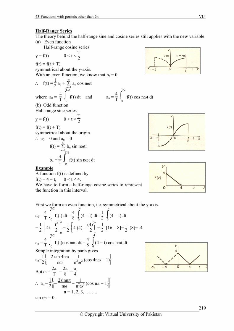
43-Functions with periods other than 2π VU
Half-Range Series The theory behind the half-range sine and cosine series still applies with the new variable. (a) Even function Half-range cosine series
y = f(t) 0 < t < T2
f(t) = f(t + T) symmetrical about the y-axis. With an even function, we know that bn = 0
f(t) = 12∴ a0 +
∞
where a0 = T
∑n=1
an cos nωt
4 ∫
T/2
0f(t) dt and an =
4T ∫
T/2
0 f(t) cos nωt dt
(b) Odd function Half-range sine series
y = f(t) 0 < t < T2
f(t) = f(t + T) al about the origin.
∴
f(t) = ∞∑ n ωt;
T
symmetric a0 = 0 and an = 0
b sin nx=1
bn = 4
∫T/2
f(t) si0
n nωt dt
Example A function f(t) is defined by f(t) = 4 − t, 0 < t < 4. We have to form a half-range cosine series to represent the function in this interval.
First we form an even function, i.e. symmetrical about the y-axis.
a0 = 4T ∫
T/2
0f1(t) dt =
48 ∫
4
0(4 − t) dt=
12 ∫
4
0(4 − t) dt
= 12 ⎪⎪
⎪⎪⎪⎪4t −
t2
2
4
0 =
12 ⎣⎢
⎡⎦⎥⎤4 (4) −
(4)2
2 = 12 [16 − 8]=
12 (8)= 4
an = 4T ∫
T/2
0f1(t)cos nωt dt =
48 ∫
4
0(4 − t) cos nωt dt
Simple integration by parts gives
an=12
⎩⎪⎨⎪⎧
⎭⎪⎬⎪⎫
− 2 sin 4nω
nω − 1
n2ω2 (cos 4nω − 1)
But ω = 2πT =
2π8 =
π4
∴ an = 12
⎩⎪⎨⎪⎧
⎭⎪⎬⎪⎫
− 2sinnπ
nω − 1
n2ω2 (cos nπ − 1)
n = 1, 2, 3, …….. in nπ = 0; s
© Copyright Virtual University of Pakistan
219

43-Functions with periods other than 2π VU
cos nπ = 1 (n even); cos nπ = − 1 (n odd) ∴ an = 0 (n even)
an = 1
n2ω2 (n odd)
∴ f(t)=2+1
ω2 ⎩⎨⎧
⎭⎬⎫cos ωt+
19cos3ωt+
125cos5ωt+… where ω =
π4 .
Example A function f(t) is defined by f(t) = 3 + t 0 < t < 2 f(t) = f(t + 4) Obtain the half-range sine series for the function in this range. Sine series required. Therefore, we form an odd function, symmetrical about the origin. a0 = 0; an = 0; T = 4 f(t) =
∞∑n=1
bn sin nωt
∴ bn = 4T ∫
T/2
0f(t) sin nωt dt= ∫
2
0 (3 + t) sin nωt dt
∫2
0 (3 + t) sin nωt dt =
⎪⎪⎪
⎪⎪⎪(3+t)cosnωt
− n ω
2
0 − ∫
2
0
cos nωt− nω dt
= (3 + 2) cos nω2
− nω − 3
− nω + 1
nω ⎪⎪⎪
⎪⎪⎪sin nωt
n ω
2
0=
3nω −
5nω cos 2 nω+
1n2ω2 ⎣⎢
⎡⎦⎥⎤sin 2nω
nω − 0
But T = 2πω ∴ ω =
2πT =
π2
= 3
nω − 5
nω cos nπ+ 1
n2ω2 ⎣⎢⎡
⎦⎥⎤sin nπ
nω
bn = 1
nω (3 − 5 cos2nω) + 1
n2ω2 (sin 2nω)
∴ bn = 1
nω (3 − 5cosnπ)+1
n2ω2 (sin nπ) = − 2
nω (n even)
= 8
nω (n odd)
∴ f(t)=
2ω⎩
⎨⎧
⎭⎬⎫4sinωt −
12sin2ωt+
43sin3ωt −
14sin4ωt..
Half-Wave Rectifier A sinusoidal voltage E sin ωt, where t is time, is passed through a half-wave rectifier that clips the negative portion of the wave Find the Fourier series of the resulting periodic functions. u(t) = 0 if − T/2 < t < 0 = E sin ωt 0 < t < T/2
here T = 2πω
© Copyright Virtual University of Pakistan
220

43-Functions with periods other than 2π VU
a0 = 2T ∫
T/2
−T/2 u(t) dt =
2T ∫
0
−T/2 0 dt +
2T ∫
T/2
0 E sin ωt dt=
2T ∫
T/2
0 E sin ωt dt=
ωπ ∫
π/ω
0 E sin ωt dt
= ωπ E
⎪⎪⎪
⎪⎪⎪− cos ω t
ω
π/ω
0
= 2Eπ
n = 2T
T/22∫
−T/2 u(t) cos n ωt dt = T ∫
0 E sin a
T/2
ωt cos n ωt dt = ωE2π ∫
π/ω
0 2 sin ωt cos n ωt dt
= ωE2π ∫
0 [sin (1+n) ωt+sin (1−n) ωt] dt
If n = 1 then integral on the right is zero and if n = 2, 3, …… then we obtain.
an=ωE2π
π/ω
⎣⎢⎡
⎦⎥⎤−
cos (1+n) ωt(1+n)ω −
cos (1−n) ωt(1−n)ω
π/ω
0 =
ωE2π
⎣⎢⎡
⎦⎥⎤−cos (1+n) π + 1
(1+n)ω + − cos (1−n) π+1
(1−n)ω
= ωE2πω
⎣⎢⎡
⎦⎥⎤−cos (1+n) π + 1
(1+n) + − cos (1−n) π+1
(1−n)
if n is odd then an = 0
if n is even then an = E2π
⎝⎜⎛
⎠⎟⎞2
1+n + 2
1−n = E2π
⎣⎢⎡
⎦⎥⎤2 − 2n + 2+2n
(1+n)(1−n) = 2E
(1−n)(1+n)π
= 2E
(1−n2)π
For bn we have
an = 2T ∫
T/2
−T/2 u(t) sin nωt dt =
2T ∫
T/2
0 E sin ωt sin nωt dt= −
ωE2π ∫
π/ω
0 − 2 sin ωt sin nωt dt
= − ωE2π ∫
π/ω
0 [cos(1+n)ωt−cos(1−n)ωt] dt
If n = 1
bn = − ωE2π ∫
π/ω
[cos 2ωt−1] dt= − ωE
0 2π ⎪⎪⎪⎪⎪sin 2ωt
ω⎪ 2 − tπ/ω
= − ωE
02π (− π/ω) = E/2
if n ≠ 1
bn =−ωE2π ∫
π/ω
0[cos(1+n)ωt−cos(1−n)ωt] dt= −
ωE2π
⎣⎢⎡
⎦⎥⎤sin(1+n) ωt
(1+n)ω − sin (1−n) ωt
(1−n)ω
π/ω
0
= − ωE2π
⎣⎢⎡
⎦⎥⎤sin(1+n) π
(1+n)ω − sin (1−n) π
(1−n)ω = 0 for n = 2, 3, 4, ........
2u (t) = 1 a0 +
∞∑n=2
an cos nωt
u(t) = Eπ +
E2 sin ωt −
2Eπ
⎝⎜⎛
⎠⎟⎞1
1.3 cos 2ωt + 1
3.5 cos 4ωt + ...
Lecture No -44 Laplace Transforms
© Copyright Virtual University of Pakistan
221

44-Laplace transforms VU
L{e3t} = 1
s − 3 ;L {t3} = 3!s4 ;L{2sin 3t + cos 3t} =
s + 6s2 + 9
And -1 3 -1 3 -14 2
1 3! 6L { } ; L { } ;L { } 2sin 3 cos33 9
t se t ts s s
t+= = = +
− +
34
3!{ }L ts
=We show that For this consider the integral
33 3 3 2 2
0 00 0
1 3( ) [ ] 3st
st st stst
e t
0
L t t e dt t t e dt t e dts s se s
∞ ∞−∞− ∞ − −
= = − = +− −∫ ∫
∞−∫
220 0
0 0 0
3 2 3 2 3.2 10 { } {sst st
st st ste et te dt te dt t e dts s s s s s s s
∞ ∞− −∞ ∞− −= + + = = +
− −∫ ∫ ∫ }−
3 3 4 4 400 0
3.2 3.2 1 3.2.1 3.2.1 3.2.1 3!( ) (0 1)st st ste dt e s dt es s s s s s
∞ ∞∞− − −− − −
= = − = = − =∫ ∫ 4s=
So that 34
3!{ }L ts
=
Laplace Transform The Laplace Transform of a function F(t) is denoted by L{F(t)} and is defined as the integral of F(t) ste− between the limits t=0 and t = ∞
L{F(t)}=
In all cases, the constant parameter s is assumed to be positive and large enough to ensure that the product F(t)
0
( ) .ste F t dt∞
−∫
ste− converges to zero as t → ∞ , what ever the function F(t). In determining the transform of any function , you will appreciate that the limits are substituted for t, so that the result will be a function of s.
That is Laplace Transform of F(t) = a (constant).
0 0
)= ae dt a e dt
0
L(a
{0 1}
st st
ste a aas s s
∞ ∞− −
−∞
=
−= = − =
−
∫ ∫
Example
form ate that F(t)= ate where a is a consFind the laplace transform of the tant. ( )
( )0
0 0
( ) [ ]( )
s a tat at st s a t eL e e e dt e dt
s a
∞ ∞ − −− − −= = =
− −∫ ∫ ∞
( )
1 1= , s > a
1 1= [0 1]=
s a ts a e
s a s a
−⎡ ⎤− ⎢ ⎥− ⎣ ⎦
− −− −
1{ }atL e
s a=
−
So we already have two standard transforms
© Copyright Virtual University of Pakistan
222

44-Laplace transforms VU
as
; at 1L{e }= ;s-a
L{a}=
4L{4}= s
; 4t 1L{e }= ;s-4
-5L{-5}= s
; -2t 1L{e }= ;s+2
Laplace transform is always a function of s. Complex Numbers Power of i Every time a factor occurs , it can be replace by the factor 1, so that the power of i is
duced to one of the four results above.
Complex Numbers
4ire
z = 3+ 5 i , is called a complex number where 3 is real part and 5 is imaginary part
of the complex number. In general z = a+ b i , is called a complex number where a is real part and b is
imaginary part of the complex number. So, Complex Number = (Real Part )+ i (Imaginary Part)
Conjugate complex numbers For a complex number a + i b , the complex number a - i b is called the conjugate of a + i b. Conjugate complex numbers are identical except the signs in the middle for the brackets.
• (4 + 5 i) and (4 - 5 i) are conjugate complex numbers • (6 + 2 i) and (2 + 6 i) are not conjugate complex numbers • (5 - 3 i) and (-5 +3 i) are not conjugate complex numbers
Remember The product of complex number by its conjugate is always entirely real. (3 + 4 i ) (3 - 4 i ) = 9 + 16 = 25 (a+ b i ) (a - bi ) =
2 2a b+
Euler Formaula As we know that the series expansion of ,cos x and sin x are given as xe
2 3 4
1 ..............2! 3! 4!
x x x xe x= + + + + +
2 4 6
cos 1 ..............2! 4! 6!x x xx = − + − +
3 5 7
sin ..............3! 5! 7!x x xx x= − + − +
Replace x by (it) , we get
i = 1. i = i 20 = ( i 4 ) 5 = (1) 5 = 1 i 30 = ( i 4 ) 7 i 2 = (1) 7 ( − 1) = 1 (
i 9 = ( i 4 ) 2 i = (1) 2 i
− 1) = − 1i 15 = ( i 4 ) 3 i 3 = 1 ( − i ) = − i
© Copyright Virtual University of Pakistan
223

44-Laplace transforms VU
2 3 4( ) ( ) ( ) ( )1 ( ) ..............
2! 3! 4!it it it ite it= + + + + +
2 3 4 5 6 7( ) ( ) ( ) ( ) ( ) ( ) ( )1 ( ) ..............
2! 3! 4! 5! 6! 7!it t i t t i t t i te it= + − − + + − − +
2 4 6 3 5 7( ) ( ) ( ) ( ) ( ) ( ) ( )[1 ..............] [ ..............]
2! 4! 6! 3! 5! 7!it t t t t t te i t= − + − + + − + − +
where
cos t =2 4 6( ) ( ) ( )1 ..............t t t
− + − + 2! 4! 6!
in t = s 3 5( ) ( ) ( )t t 7
..............3! 5! 7!
tt − + − +
t i t= +
R( )= cost and I( ) = sin t The Laplace transform of F(t) = sin at
cos sinite
ite ite
( )( )
0 0 0
L(Sin at) = L(I( )) ( )
1 1(0 1)( ) ( )
s ia tiat iat st s ia t ee I e e dt I e dt I
s ia
I Is ia s ia
∞∞ ∞ − −− − −
⎧ ⎫⎡ ⎤⎪ ⎪= = = ⎨ ⎬⎢ ⎥− −⎣ ⎦⎪ ⎪⎩ ⎭⎧ ⎫ ⎧ ⎫
= − =⎨ ⎬ ⎨ ⎬− − −⎩ ⎭ ⎩ ⎭
∫ ∫
2 2 2 2 2 2{sin } { } [ ]s ia s aL at I I is a s a s a
+= = +
+ + +
2 2{sin } aL ats a
=+
∴
We can use the same method to determined to determine L{cos at }. Since cos at is the real part of , written as R( ) iate iate
2 2 2 2 2 2
2 2{cos }L ats a
=+
{cos } { } [ ]s ia s aL at R R is a s a s as
+= = +
+ + +
The Transform of F(t) = tn where n is a positive integer.
By the definition integrating by parts n
0
L(t ) = n stt e dt∞
−∫
n 1
00 00
1L(t ) = st
n st n n st n st n ste n nt e dt t t e dt t e t e dts s s s
∞∞ ∞− ∞− − − −⎡ ⎤⎡ ⎤= + = − +⎢ ⎥ ⎣ ⎦−⎣ ⎦
∫ ∫ 1
0
∞− −∫
0
0 0 0st
n et−⎡ ⎤s
∞
∴ = − =−⎣ ⎦
⎢ ⎥1
0
{ }n n sn tL t t es
∞− − dt∴ = ∫ -----------------(1)
you will notice that is identical to except that n is replaced by (n-1) 1
0
n stt e dt∞
− −∫0
n stt e dt∞
−∫
© Copyright Virtual University of Pakistan
224

44-Laplace transforms VU
− and the result (1) becomes 11
0 0
,n st n stn nif I t e dt then I t e dt
∞ ∞− −
−= =∫ ∫If
1n nnI Is −=
This is reduction formula and , if we now replace n by (n-1) we get
1 21
n nn I
s− −
−=
we replace n by (n-1) again in this last result , we have
I
If
2 32
n nn I
s− −
−= I
1 2 30
43
no I t e dt I I I Is s s s s s s s s s
∞−
− − − −
− − − − − −= = = = =∫
o finally, we have
1 1 2 1 2. . . . . .n stn n n n
n n n n n n n n n nS
S
01 2 3 4 2 1. . . . ............... .n
n n n n nI Is s s s s s s
− − − −=
But 0
01{ } {1}I L t Ls
= = =
0 1
1 2 3 4 2 1 !...............n n
n n n n n nI Is s s s s s s s +
− − − −= =
1
!n n{ } nL ts +=
2 32 3 4
1 2! 3!{ } ; { } ; { }L t L t L ts s s
= = = 4
6s
=
ransform of F(t) = sinh at and F(t) = cosh at.Laplace T
Starting from the exponential definitions of sinh at and cosh at
1 1. . sinhi e ( ) cosh ( )2 2
at at at atat e e and at e e− −= − = +
We proceed as follow
) ( ) sinha F t at=
( ) ( )
0 0 0 0
1 1 1Sinh at = sinh ( ) ( ) ( )2 2 2
st at at st at st at st s a t s a tat e dt e e e dt e e e e dt e e dt∞ ∞ ∞ ∞
− − − − − − − − − += − = − = −∫ ∫ ∫ ∫
( ) ( )
0 0
2 2 2 2
1 1 1 1 1 1 1(0 1) (0 1)2 ( ) ( ) 2 ( ) ( ) 2 ( ) ( )
1 1 22 ( )( ) 2
s a t s a te es a s a s a s a s a s a
s a s a a as a s a s a s a
∞ ∞− − − +⎧ ⎫⎡ ⎤ ⎡ ⎤ ⎧ ⎫ ⎧ ⎫⎪ ⎪= − = − − − = −⎨ ⎬ ⎨ ⎬ ⎨ ⎬⎢ ⎥ ⎢ ⎥− − − + − − − + − +⎩ ⎭⎣ ⎦ ⎣ ⎦ ⎩ ⎭⎪ ⎪⎩ ⎭⎧ ⎫+ − + ⎧ ⎫ ⎧ ⎫= = =⎨ ⎬ ⎨ ⎬ ⎨ ⎬− + − −⎩ ⎭ ⎩ ⎭⎩ ⎭
) ( ) coshb F t at=
© Copyright Virtual University of Pakistan
225

44-Laplace transforms VU
( ) ( )
0 0 0
( ) ( )
0 0
1 1 1L(cosh at) = L( ( + )) ( )2 2 2
1 1 1 1 1 1 1(0 1) (0 1)2 ( ) ( ) 2 ( ) ( ) 2 ( ) ( )
at at at at st s a t s a t
s a t s a t
e e e e e dt e dt e dt
e es a s a s a s a s a s a
∞ ∞ ∞− − − − − +
∞ ∞− − − +
⎡ ⎤= + = +⎢ ⎥
⎣ ⎦⎧ ⎫⎡ ⎤ ⎡ ⎤ ⎧ ⎫ ⎧ ⎫⎪ ⎪= + = − + − = +⎨ ⎬ ⎨ ⎬ ⎨⎢ ⎥ ⎢ ⎥− − − + − − − + − +⎩ ⎭⎣ ⎦ ⎣ ⎦ ⎩⎪ ⎪⎩ ⎭
∫ ∫ ∫
2 2 2 2
1 1 22 ( )( ) 2
s a s a s ss a s a s a s a
⎬⎭
⎧ ⎫+ + − ⎧ ⎫ ⎧ ⎫= = =⎨ ⎬ ⎨ ⎬ ⎨ ⎬− + − −⎩ ⎭ ⎩ ⎭⎩ ⎭
2 2L(cosh at) ss a
⎧ ⎫= ⎨ ⎬−⎩ ⎭
Several Standard Results
1
1 !{ } ; { } ; { }at nn
a nL a L e L ts s a s += = =
−
2 2 2{sin } ; {cos }a sL at L ats a s a
= =+ +
2
2 2 2 2{sinh } ; {cosh }a sL at L ats a s a
= =− −
e can , of course, combine these transforms by adding or subtracting as necessary , but ey must not be multiplied together to form the transform of a product.
xample
Wth E
2 2 2
3 6) {2sin 3 cos3 } 2 (sin 3 ) (cos3 ) 2.9 9
s s9
L t t L t L ts s s
++ = + = + =
+ + + a
2 22 2
2
2
1 4) {4 3cosh 4 } 4 ( ) (3cosh 4 ) 4. 3.2 16 2
7 6 64( 2)( 16)
t t s sb L e t L e L ts s s s
s ss s
+ = + = + = +3
16− − − −− −
=− −
© Copyright Virtual University of Pakistan
226

45-Theorems VU
Lecture No -45 Theorems Theorem 1 The First Shift Theorem The first Shift theorem states that if L{F(t)}= f(s) then L{e(-at) F(t)}= f(s+a) The transform L{e(-at) F(t)} is thus the same as L{F(t)} with s everywhere in the result replaced by (s+a) Example
2
2L{sin 2t}= s 4+
then -3t2 2
2 2L{e sin 2t}= (s+3) 4 6 13s s
=+ + +
Example
2 23
2{ } ; { }t4L t L ts
= e is the same with s replaced by (s-4)
So 2 43
2{ }( 4)
tL t es
=−
Theorem 2 Multiplying by t
If L{F(t)}= f(s) then { ( ( )} { ( )}dL t F t f sds
= −
2
2L{sin 2t}= s 4+
Example
2 2
d 2 4L{t sin 2t} = -ds ( 4) ( 4)
ss s
⎡ ⎤=⎢ ⎥+ +⎣ ⎦
And 2
Example ( )2 2 2 2
2 2 2 2 2
( 9) 2 9 2 9{ cos3 }9 ( 9) ( 9) ( 9)
s s sd s s s sL t tds s s s s
− −2 2
− − +⎛ ⎞= − = − = − =⎜ ⎟− − −⎝ ⎠
−We could, if necessary, take this a stage further and find
2 2
2 2 2 3
9 2 ( 27{ cos3 }( 9) ( 9)
d s s sL t tds s s
⎛ ⎞+ += − =⎜ ⎟− −⎝ ⎠
)
Theorem Obviously extends the range of function that we can deal with. So, in general
}= f(s) then { ( ( )} ( 1) { ( )}n
n nn
dL t F t f sds
= − If L{F(t)
Theorem Dividing by t
If L{F(t)}= f(s) then ( ){ } ( )s
F tL f s dst
∞
= ∫
Example Determine sin at{ }Lt
2 2{sin } as L at =As a+
1 12 2
sin{ } tan ( ) tan ( ) tan ( )2ss
at a s s aL dst s a a a
π∞∞− −⎡ ⎤ 1
s−∴ = = = − =⎢ ⎥+ ⎣ ⎦∫
© Copyright Virtual University of Pakistan
227

45-Theorems VU
Example Determine 1-cos 2tL{ }t
As 2L{1-cos 2t}=4s s
−+
1 s
Then by Theorem 3,
2 22
s 4 2 2 22
2 2 22
1 1L{ } = ( ) ln ln( 4) .2 ln ln( 4)t
1 1 1ln ln( 4) ln ln( 4) ln2 2 2 2 ( 4)
1-cos 2t 1 1
1
s s
ss s
ds s s s s
ss s s ss
ss s
∞ ∞
∞∞∞
∞ ⎡ ⎤ ⎡ ⎤− = − + = − +⎢ ⎥ ⎢+ ⎥⎣ ⎦ ⎣∫ ⎦
⎡ ⎤⎡ ⎤ ⎡ ⎤= − + = − + = ⎢ ⎥⎣ ⎦⎢ ⎥ +⎣ ⎦ ⎣ ⎦
2
2ln ln1 0( 4)
sWhen s thens
→ ∞ → =+
12 2 2
2 2 2s
1-cos 2t 1 1 4L{ } = ( ) ln ln lnt 4 2 ( 4) ( 4)
s s sdss s s s s
−∞ ⎡ ⎤ ⎡ ⎤ +− = − = =⎢ ⎥ ⎢ ⎥+ + +⎣ ⎦ ⎣ ⎦
∫ 2
2
s
Standard Forms
Theorem 1
The First Shift Theorem If L{F(t)}= f(s) then L{e(-at) F(t)}= f(s+a) Theorem 2 Multiplying by t
If L{F(t)}= f(s) then { ( ( )} { ( )}dL t F t f sds
= −
Theorem 3 Dividing by t
If L{F(t)}= f(s) then ( ){ } ( )s
F tL f s dst
∞
= ∫
Provided 0
( ) .t
F tLim existst→
⎧ ⎫⎨ ⎬⎩ ⎭
F(t) L {F(t)} = f(s) a a
s
e 1− a
at s
s in at as2 + a2
c os at as2 + a2
s inh at as2 − a2
c osh at ss2 − a2
t n n!sn+1
(n a positive integer)
© Copyright Virtual University of Pakistan
228

45-Theorems VU
Inverse Transforms Here we have the reverse process i.e. given a Laplace transform, we have to find the
function of t to which it belongs. For example, we know that 2 2
as a+
is the Laplace
Transform of sin at , so we can now write 12 2 sinaL at
s a− ⎡ ⎤ =⎢ ⎥+⎣ ⎦
, the symbol L-1
indicating the inverse transform and not a reciprocal. 1 2
12
1( )2
( ) cos525
ta L es
sb L ts
− −
−
⎧ ⎫ =⎨ ⎬−⎩ ⎭
⎧ ⎫ =⎨ ⎬+⎩ ⎭
1
12
4( ) 4
12( ) 4sinh 39
c Ls
d Ls
−
−
⎧ ⎫ =⎨ ⎬⎩ ⎭⎧ ⎫ =⎨ ⎬−⎩ ⎭
t
But what about 12
36
sLs s
− ⎧ ⎫⎨ ⎬− −⎩ ⎭
, it happens that we can write 2
36
ss s− −
as the sum of
two simpler functions 1 12 3s s
++ −
which , of course , makes all the difference , since we
can now proceed. 12
3s 1 1 2 31 1 26 2 3
t tL L L e es s s s
− − −⎫ ⎧ ⎫ ⎧ ⎫= + = +⎬ ⎨ ⎬ ⎨ ⎬− − + −⎩ ⎭ ⎩ ⎭ ⎩ ⎭
Rules of Partial Fractions
− ⎧⎨
1. The numerator must be of lower degree than denominator. If it is not , then we first divide out.
inator into its prime factors. These determine the shapes of the n.
3. A linear factor (s+a) gives a partial fraction
2. Factorise the denompartial fractio
As a+
is a constant to be determined.
4. A repeated factor (s+a)2 gives 2( )A B
s a s a+
+ +
2 3( ) ( )A B C
s a s a s a+ +
+ + + 5. Similarly (s+a)3 gives
6. A quadratic Factor ( q ) gives 2s ps+ + 2
Ps Qs ps q
++ +
7. Repeated quadratic Factor gives 2 2( )s ps q+ + 2 2( )Ps Q Rs T
s ps q s ps q 2
+ ++
+ + + +
So 19( 2)( 5
ss s
−− + )
has partial fraction of the form ( 2) ( 5)
A Bs s
+− +
and 2
2
3 4 11( 3)( 2)
s ss s
− ++ −
has partial fraction 2( 3) ( 2) ( 2)A B C
s s s+ +
+ − −
© Copyright Virtual University of Pakistan
229

45-Theorems VU
Example
To determine 12
5 112
sLs s
− +⎧ ⎫⎨ ⎬− −⎩ ⎭
a) First we check that the numerator is of lower degree than the denominator. In fact this is so.
b) Factories the denominator
2
5 1 5 1s s+ +12 ( 4)( 3) ( 4) ( 3)
A Bs s s s s s
= = +− − − + − +
We therefore have an identity
2
5 112 ( 4) ( 3)
s As s s s
+= +
− − − + B
which is true for any value of s we care to substitute If we multiply through by the denominator ( 2 12s s− − ) we have
ena valu i) Let (s -4) =0 that is s = 4 therefore 21 = A(7) + B(0) ⇒ A= 3 ii) Let (s + 3) =0 that is s = -3 therefore B = 2
So
5s + 1 ≡ A(s + 3) + B( 4)s -
We now substitute cov nt es for s
2
5 1 3 212 ( 4) ( 3)
ss s s s
+= +
− − − +
1 4 32 3 2
12t t5 1sL e e
s s− −+⎧ ⎫ = +⎨ ⎬− −
Ex
⎩ ⎭
ample Determined 1 9 8sL− −⎧ ⎫⎨ ⎬ 2 2s s−⎩ ⎭
2
9 8{ ( )}2
sL F ts s
−=
−
a) Numerator of first degree ; denominator of second degree.
b) 2
9 82 2
s As s s s
−= +
− − B
c) Multiply by s(s – 2 ) ∴9 s -8 ≡ A(s - 2) + B (s) d) Put s = 0 ∴ -8 ≡ A( - 2) + B (0) ∴Α = 4
∴ 10 = Α ( 0 ) + Β ( 0 ) ∴B = 5
∴
e) Put s – 2 , i.e. s = 2
-1 2t4 5F(t) = L = 4 + 5e s s-2
⎧ ⎫+⎨ ⎬⎩ ⎭
© Copyright Virtual University of Pakistan
230

45-Theorems VU
© Copyright Virtual University of Pakistan
231
ransforms Of Derivatives T
et F/(t) denote the first derivative of F(t) with respect to t , F//(t) denote the second derivative of F(t) with respect to t, etc.
Then by definition ,
Integrating By Parts st
st
L
/ -st /
0
L{ F (t)}= e F (t)dt∞
∫
/ -
00
L{ F (t)}= ( ) ( )( e )dtste F t F t s∞
∞−⎡ ⎤ − −⎣ ⎦ ∫
when t 0, ( ) 0ste F t−→ →
/ -
0
L{ F (t)}=- (0) e ( )dtF s F t∞
+ ∫
/L{ F (t)}=- (0) L{ F (t)}F s+
// / / /L{ F (t)}=- (0) L{ F (t)}=- (0) - (0) L{ F (t)}F s F s F s⎡ ⎤+ + +⎣ ⎦
T a b le o f in v e r s e t r a n s f o r m s S ta n d a r d t r a n s f o r m s f ( s ) F ( t ) a
s a
1s + a e - a t
n !n + 1s t n
( n a p o s i t i v e i n t e g e r )
1
// 2 /L{ F (t)}= L{ F(t)}- (0) (0)s sF F+
/// 3 2 / //L{ F (t)}= L{ F(t)}- (0) (0) (0)s s F sF F− −
iv 4 3 2 / // ///L{ F (t)}= L{ F(t)}- (0) (0) (0) (0)s s F s F sF F− − −
s n ( n − 1 ) !t n - 1
( n a p o s i t i v e i n t e g e r )
as 2 + a 2 s i n a t
ss 2 + a 2 C o s a t
as 2 − a 2
S in h a t
ss 2 − a 2
C o s a x

45-Theorems VU
© Copyright Virtual University of Pakistan
232
Differential Equation And Its Solution
2 4dx xdt
− = -----------------(1)
Its Solution is 2tx = -2 + 3e , To verify it we find dxdt
26 tdx edt
= then
2 2
2 2
2 6 2( 2 3 )
6 4 6 4
t t
t t
dx x e edt
e e
− = − − +
= + − =
So equation (1) is satisfied. Hence 2tx = -2 + 3e is solution of 2 4dx xdt
− =
Example Solve the differential equation 2 4dx xdt
− = given that at t = 0 , x = 1
Taking Laplace transform as 4( ( )) 2 ( ( )) (4) ( ( )) 2 ( ( )) (4) ( ( )) (0) 2 ( ( ))d dL x t L x t L L x t L x t L sL x t x L x t
dt dt s⎡ ⎤ ⎡ ⎤− = ⇒ − = ⇒ − − =⎢ ⎥ ⎢ ⎥⎣ ⎦ ⎣ ⎦
4 4 4 4( 2) ( ( )) (0) ( 2) ( ( )) 1 ( 2) ( ( )) 1 ( 2) ( ( )) ss L x t x s L x t s L x t s L x ts s s s
+− − = ⇒ − − = ⇒ − = + ⇒ − =
14 4( ( )) ( )( 2) ( 2)
s sL x t x t Ls s s s
− ⎡ ⎤+ +⇒ = ⇒ = ⎢ ⎥− −⎣ ⎦
-----------------------(1)
First we do the partial fraction of 4( 2)
ss s
+−
4( 2) ( 2)
s A Bs s s s
+= +
− −
4 ( 2) ( )s A s B s⇒ + = − + -----------------(2)
Put s = 0 in equation (2) ; 4 = -2A ; A = -2 Put s = 2 in equation (2) ; 6 = B(2) ; B = 3
4 2 3( 2) 2
sSos s s s
+ −= +
− −
Equation # (1) becomes 1 1 1 24 2 3( ) 2 3
( 2) 2tsx t L L L e
s s s s− − −⎡ ⎤+ −⎡ ⎤ ⎡ ⎤= = + = − +⎢ ⎥ ⎢ ⎥ ⎢ ⎥− −⎣ ⎦ ⎣ ⎦⎣ ⎦
Solution of differential equation by laplace transforms To solve a differential equation by Laplace transforms, we go through Laplace transforms, we go through four distinct stages.
(a) Re- write the equation in term of Laplace transforms. (b) Insert the given initial conditions. (c) Rearrange the equation algebraically to give the transform of the solution.

45-Theorems VU
© Copyright Virtual University of Pakistan
233
(d) Determine the inverse transform to obtain the particular solution. Solve the equation
23
2 3 2 2 td x d x x edt dt
− + = given that at t = 0 , x = 5 and 7dxdt
= // / 3( ) 3 ( ) 2 ( ) 2 tx t x t x t e− + =
Given x ( 0 ) = 5 , xP
/P ( 0 ) = 7
( )// / 3( ) 3 ( ( )) 2 ( ( )) 2 ( )tL x t L x t L x t L e− + =
2 / 2{ ( )} (0) (0) 3{ ( ( )) (0)} 2 ( )3
s L x t s x x s L x t x L x ts
− − − − + =−
We rewrite the equation in term of its transforms.
[ ]2
32 3 2 2 td x d xL L L x L e
dt dt⎡ ⎤ ⎡ ⎤
⎡ ⎤− + =⎢ ⎥ ⎢ ⎥ ⎣ ⎦⎣ ⎦ ⎣ ⎦
2 / 3[ ( ( )) (0) (0)] 3[ ( ( )) (0) ] 2 ( )ts L x t s x x s L x t x L e⎡ ⎤− − − − +⎣ ⎦
At t = 0 , x = 5 , 7dxdt
=
So x ( 0 ) = 5 , x P
/P( 0 ) = 7
2 2( ( )) (5) 7 3{ ( ( )) 3(5)} 2 ( ( ))3
s L x t s sL x t L x ts
− − − + + =−
2 2( ( )) 3 ( ( )) 2 ( ( )) 8 53
s L x t sL x t L x t ss
− + = − +−
22 2 8 24 5 15( 3 2) ( ( ))
3s s ss s L x t
s− + + −
− + =−
2 22 8 24 5 15 5 23 24( ( ))( 1)( 2)( 3) ( 1)( 2)( 3)
s s s s sL x ts s s s s s
− + + − − += =
− − − − − −
Making Partial fraction of R.H.S , We have
( ( ))( 1) ( 2) ( 3)
A B CL x ts s s
= + +− − −
After solving these we get A= 3 , B = 2 and C = 0
So 3 2 0( ( ))( 1) ( 2) ( 3)
L x ts s s
= + +− − −
1 1 23 2( ) { } { } 3 2
( 1) ( 2)t tx t L L e e
s s− −= + = +
− −
3 2( ( ))( 1) ( 2)
L x ts s
= +− −