Cambio Climatico Ramsey

7/27/2019 Cambio Climatico Ramsey

http://slidepdf.com/reader/full/cambio-climatico-ramsey 1/17

Resource and Energy Economics 27 (2005) 1–17

On climate change and economic growth

Samuel Fankhauser a, Richard S.J. Tol b,c,d,∗

a European Bank for Reconstruction and Development, Hamburg University and

Centre for Marine and Atmospheric Science, Hamburg, Germanyb

Research Unit Sustainability and Global Change, Hamburg University and Centre for Marine and Atmospheric Science, Hamburg, Germanyc Institute for Environmental Studies, Vrije Universiteit, Amsterdam, The Netherlands

d Center for Integrated Study of the Human Dimensions of Global Change,

Carnegie Mellon University, Pittsburgh, PA, USA

Received 27 June 2002; received in revised form 7 January 2004; accepted 18 March 2004

Available online 9 September 2004

Abstract

The economic impact of climate change is usually measured as the extent to which the climate of

a given period affects social welfare in that period. This static approach ignores the dynamic effects

through which climate change may affect economic growth and hence future welfare. In this paper

we take a closer look at these dynamic effects, in particular saving and capital accumulation. With a

constant savings rate, a lower output due to climate change will lead to a proportionate reduction in

investment which in turn will depress future production (capital accumulation effect) and, in almost

all cases, future consumption per capita. If the savings rate is endogenous, forward looking agents

would change their savings behavior to accommodate the impact of future climate change. This

suppresses growth prospects in absolute and per capita terms (savings effect). In an endogenous

growth context, these two effects may be exacerbated through changes in labour productivity and

the rate of technical progress. Simulations using a simple climate-economy model suggest thatthe capital accumulation effect is important, especially if technological change is endogenous, and

may be larger than the direct impact of climate change. The savings effect is less pronounced. The

dynamic effects are more important, relative to the direct effects, if climate change impacts are

moderate overall. This suggests that they are more of a concern in developed countries, which are

∗ Corresponding author. Present address: ZMK, Bundesstrasse 55, Hamburg 20146, Germany.

Tel.: +49-40-42838-7007; fax: +49-40-42838-7009.

E-mail address: [email protected] (R. S.J. Tol).

0928-7655/$ – see front matter © 2004 Elsevier B.V. All rights reserved.

doi:10.1016/j.reseneeco.2004.03.003



2 S. Fankhauser, R. S.J. Tol / Resource and Energy Economics 27 (2005) 1–17

believed to be less vulnerable to climate change. The magnitude of dynamic effects is not sensitive

to the choice of discount rate.

© 2004 Elsevier B.V. All rights reserved.

JEL classification: D91; E21; O13; Q25

Keywords: Climate change; Impacts; Saving; Economic growth

1. Introduction

In most studies of the economic impact of global warming the effects of climate change

are assessed and valued separately sector by sector and then added up to form an estimate of

the overall change in social welfare (e.g., Nordhaus, 1991; Cline, 1992; Fankhauser, 1995;Tol, 1995; Mendelsohn and Neumann, 1999). This is known as the enumerative approach.1

It is well known and widely documented in the literature that this method ignores potentially

significant “horizontal interlinkages”, that is, the interaction of sectoral impacts such as the

connection between agriculture (where irrigation needs may go up) and water (where supply

may decrease). See Smith et al. (2001) and Tol et al. (2000) for a discussion.

Less well documented is the fact that the enumerative approach also neglects dynamic

interlinkages. Enumerative studies are concerned with only one time period and ask how the

climate observed in that period affects social welfare at that particular point in time. In doing

so, they ignore intertemporal effects and fail to provide information on how climate changemay affect welfare in the longer term. This paper seeks to close this gap by exploring, both

theoretically and numerically, the dynamic effects that link climate change and economic

growth.

The main dynamic effect is via capital accumulation. If we assume a constant savings

rate, the amount of investment in an economy will be reduced if climate change has a nega-

tive impact on output (and vice versa if impacts are positive). Over the longer term this will

lead to a reduction in the capital stock, a lower GDP and, in most cases, lower consump-

tion per capita. In an endogenous growth context, this capital accumulation effect may be

exacerbated if lower investment also slows down technical progress and improvements in

labour productivity or human capital accumulation.A second dynamic effect has to do with savings. In a world with perfect foresight we can

expect forward-looking agents to change their savings behavior in anticipation of future

climate change. This, too, will affect the accumulation of capital and hence growth and

future GDP. It is unclear, a priori, whether this savings effect will be positive or negative.

On the one hand, savings rates may go up because agents wish to compensate for the shortfall

in future income. On the other hand, climate change reduces the productivity of capital and,

faced with a lower rate of return, agents may prefer to invest less and consume more today.

Integrated assessment models with an economic foundation (e.g., Nordhaus, 1994; Peck

and Teisberg, 1992; Tol, 1999) usually incorporate the capital accumulation effect and

sometimes the savings effect because their design is based on neo-classical growth theory.

1 The term is due to Cline (1994).



S. Fankhauser, R. S.J. Tol / Resource and Energy Economics 27 (2005) 1–17 3

But they do not normally separate the dynamic effects explicitly. In this paper we try

to do so. Section 2 discusses the theoretical links between climate change and growth

by looking at the steady state of a stylized growth model. In Section 3 we simulate the

magnitude and direction of the dynamic effects using DICE, a relatively simple and widelyused climate-economy model (see Nordhaus, 1994). We also investigate the sensitivity to

alternative specifications of the mechanisms of growth. Section 4 estimates the effect of

climate change on the rate of growth, and Section 5 concludes.

2. A theoretical model of climate change and growth

2.1. Model description

To study the basic interlinkages between climate change and economic growth, we use

a standard Ramsey–Cass–Koopmans growth model, in which a social planner maximizes

the utility of identical consumers in the following intertemporal optimization problem:

max

∞

0u(c, T) e(n−ρ)t dt, (1)

subject to:

K = F(K, L, T) − cL − δ(T)K, (2)

L = n(T)L, L0 = 1, (3)

where u denotes the utility function, c is the per capita consumption; F the output; K the

capital, depreciating at rate δ; and ρ the discount rate.

L is labour supply, which grows at rate n, starting from an initial, normalised level of 1;

growth in labour supply is exogenous in this formulation and basically reflects changes in

population. More sophisticated models would interpret the variable as effective labour. The

growth rate n then reflects both changes in population ( p) and labour productivity ( x), n= p

+ x, with x an endogenous variable. We will look at models with endogenous productivity

improvements in the next section.

For simplicity, climate change is represented by an exogenous, time independent indi-

cator, T (for temperature). The larger T , the more pronounced are the impacts of climate

change. Climate change affects the optimization at up to four levels:

• Non-market impacts such as the amenity value of climate and the effect on recreational

and environmental assets. Non-market impacts directly affect the utility function, and we

assume them to be negative, ∂u / ∂T = uT < 0, although the impact literature has identified

potential non-market benefits as well (Smith et al., 2001).

• Market impacts, such as a change in agricultural yields, which enter the production func-

tion. Again we assume the net impact to be negative, ∂F / ∂T = F T < 0, notwithstanding

arguments in the more recent literature that market impacts may initially be positive atleast for some regions (e.g., Mendelsohn and Neumann, 1999; Tol, 1999). Output could

fall either because productivity falls or because output is destroyed by climate change.




• Health and mortality impacts associated with more widespread diseases such as malaria.

These affect population growth2 and are believed to be predominantly negative, ∂n/ ∂T

= nT < 0 (McMichael et al., 2001).

• The impact on the longevity of capital. This effect is less established in the literature,although some adaptation studies (e.g., Fankhauser et al., 1999) have pointed out that

a continuously changing climate will require more frequent adjustments in the capital

stock, especially with respect to defensive expenditures (e.g., the strengthening of sea

walls and dykes). More frequent extreme events (e.g., storms) will also affect the longevity

of capital. This can be captured in an increased speed of capital depreciation, ∂δ / ∂T = δT

> 0.

If output is homogeneous of degree one in labour and capital, we have

k =

K

L , k =

K

L −

K

L

L

L , f(k) = F(k, 1,T), Lf (k) = F(K, L, T), (4)

and (2) and (3) can be combined to

k = f − c − δk − nk . (5)

Solving the model yields, after some manipulation:

c = −uc

ucc

(f k − δ − ρ), (6)

where subscripts denote derivatives. Eqs. (6) and (5) are the two equations of motion driving

the system. The steady state is defined by c = k = 0, which implies

f k = δ + ρ, (7)

c = f − δk − nk . (8)

2.2. Capital accumulation

We first look at the impact of climate change on capital. To isolate the capital accumulation

effect we keep the savings rate exogenously fixed. Agents are not allowed to adjust their

savings behavior in response to climate change. With the savings rate set at a constant

fraction of output,¯s

=1

−c/f Eq. (8) becomes

sf = (δ + n)k. (9)

This is the familiar steady-state condition of the Solow–Swan model (see for example Barro

and Sala-I-Martin, 1995). By totally differentiating Eq. (9) we get

∂k

∂T =

k(δT + nT ) − sf T

sf k − δ − n. (10)

Note that the denominator in this expression is negative. Because the savings function,

sf(k), is concave it intersects the linear depreciation schedule, (δ + n)k, from above at the

steady state. That is, it has a flatter slope,¯sf k < (δ

+n).

2 In more sophisticated models health impacts also affect the productivity of the labour force. This would count

as a market impact, again with ∂F / ∂T = F T < 0.




Eq. (10) tells us that the four channels of climate change impact identified earlier affect

the capital-labour ratio as follows:

• Non-market impacts, uT < 0, do not affect capital accumulation because climate changeis exogenous and thus acts only to rescale utility.3

• Market impacts in the form of a reduction in output, f T < 0, have a negative effect. If less

output is produced, a lower absolute amount can be devoted to capital accumulation, and

the capital-labour ratio, k , is reduced.

• However, the amount of labour available in the steady state is also reduced because of

the health impacts of climate change, nT < 0. This will push up the capital-labour ratio

and may at least partially offset the market impacts.

• The capital stock is further reduced because it is depreciating faster, ␦T > 0, which,

everything else being equal, will again reduce the capital-labour ratio.

The overall effect of climate change on the accumulation of capital is in principle ambiguous.

However, it seems safe to speculate that the capital accumulation effect will probably be

negative. A cursory look at the impact literature suggests that the market and depreciation

effects are likely to outweigh the health effect in most countries. The exception may be

some of the most vulnerable poor countries, where the health impacts of climate change

tend to be disproportionately high and the amount of capital per worker disproportionately

low. We also know that the effect on the absolute capital stock, K , is clearly negative (since

we can ignore the health impact in this case as it works through the denominator of the

capital-labour ratio).

2.3. Saving

We now turn to saving. If gross saving per capita, sG, is defined as output minus con-

sumption, we can use Eq. (8) to derive

sG= f − c = (δ + n)k. (11)

Differentiating sG with respect to T yields

∂sG

∂T

= (δT + nT )k + (δ + n)∂k

∂T

. (12)

The impact of climate change on capital accumulation can be derived by totally differenti-

ating (7), which yields the following expression for ∂k / ∂T :

∂k

∂T =

δT − f kT

f kk

. (13)

By substituting (13) back into (12) we derive

∂sG

∂T = δT

k +

δ + n

f kk

+ nT k −

(δ + n)f kT

f kk

. (14)

3 This is true for strictlynon-market impacts only. However,non-market impactstypically also include landscapes

and health-impacts that have an effect on the markets for recreation and health care. Such effects are here included

under market impacts.




Eq. (14) tells us that the four climate change impacts of the model affect saving in the

following ways:

• Non-market impacts, uT < 0, do not affect saving for the same reason as they did notaffect capital accumulation. Climate change is exogenous and acts only to rescale utility.

• Assuming market impacts are multiplicative (as in DICE), their effect on saving is nega-

tive. Climate change reduces the marginal product of capital, f kT < 0, which means that

the return on capital is lower. Faced with a lower capital productivity, consumers decide

to reduce investment and the capital stock declines (recall that f kk < 0).

• The health impacts of climate change also affect saving negatively, nT < 0. If there are

fewer people in the future they will need less capital.

• The impact of accelerated capital depreciation, δT > 0, is ambiguous. On the one hand,

savers wish to compensate for the faster deterioration of their capital stock by providing

additional funds. On the other hand, they are discouraged from doing so because moreshort-lived capital also means lower returns: The benefit stream associated with a given

investment is cut short.

Two features of Eqs. (12)–(14) are worth pointing out before we move to their numerical

estimation. The first observation has to do with the difference between gross and net savings.

The direction of the (gross) savings effect in Eq. (14) is undetermined because the capital

depreciation effect, δT > 0, is partially positive. Agents will save more to compensate for

accelerated capital depreciation and at least in theory this could offset the other, negative

effects of climate change on saving. However, if instead of gross savings we look at net

savings, sN

= nk , Eq. (14) simplifies to

∂sN

∂T = nT k + n

δT − f kT

f kk

< 0, (15)

an expression that is unambiguously negative. Savers will not set aside enough extra money

to compensate for all negative effects. They will consciously cut net investment with a view

to reduce the capital stock. Unlike in the case with a fixed savings rate, the impact of climate

change on capital accumulation Eq. (13) is clearly negative.

The second point worth noting is on the discount rate. Intuitively, we would expect that a

lower discount rate would lead to higher savings in the face of climate change. People with

a higher regard for future welfare would save more to compensate for the expected losses.

However, the opposite is the case. A lower discount rate (parameter ρ) will, obviously, lead

to higher steady state saving. However, introducing climate change at this higher saving

level will trigger a more strongly negative reaction. With a lower discount rate, people will

respond more strongly to the lower future productivity of capital and cut savings by more.

This is because the marginal productivity of capital is lower when capital is abundant, so

that investments can be cut with smaller repercussions for production. We can see this by

substituting Eq. (7) into (12):

∂sG

∂T = (δT + nT )k + (f k − ρ + n)∂k

∂T . (16)

The lower ρ in Eq. (16), the more negative the expression becomes.




3. The magnitude of dynamic effects

To gain further insights on the relative importance of the dynamic effects we now turn to

a numerical model of climate change. We choose the well-known DICE model developedby Nordhaus (1994) as the basis of our simulations. It should be noted that DICE does not

distinguish the four channels through which climate change affects growth we identified

in Section 2. Instead, it assumes that all impacts are channeled through the production

function. This is acceptable as the concern in this section is less with the mechanics of the

dynamic effects and the channels through which they arise, than with their magnitude and

importance.4 DICE is also a model of the world economy, we can easily interpret the results

as those of a small country without control over atmospheric CO2 concentrations.5

Some adjustments to the model are, however, needed to make it suitable for our purposes.

We use the functional forms and parameters as in DICE, but exclude the option of emission

reduction and fix the temperature scenario. To distinguish between the savings and capital

accumulation effect, we run the model in two different modes, associated with different

growth models (see Barro and Sala-I-Martin, 1995; Romer, 1996; and Appendix A):

• The Solow–Swan specification: In the Solow–Swan growth model saving is an exoge-

nously given fraction of income. Technological progress is also exogenous. We can use

this model to isolate the capital accumulation effect by comparing its GDP predictions

with the direct impacts of climate change. The exogenous savings rate was derived from

the DICE base run in which there is no climate change. This savings rate is optimal, given

the DICE parameters, in a world without climate change.

• The Ramsey–Cass–Koopmans specification: This is the original model structure of DICE(Nordhaus, 1994) and similar to the theoretical model of Section 2. Savings rates are de-

termined endogenously, and are hence affected by climate change. Technical progress on

the other hand is exogenous. The comparison of this specification with the Solow–Swan

model will provide insights into the magnitude of the savings effect.

In addition, we use two endogenous growth specifications to see how the dynamic effects

differ if investment decisions also affect human capital accumulation and technical progress.

Again, they can be associated with two standard growth models (see Appendix A f or detailed

specifications):

• The Mankiw–Romer–Weil specification: In this model (due to Mankiw et al., 1992) tech-

nological progress is exogenous and savings are given. The crucial distinction of this

model is that, besides physical capital, the model also includes human capital. Compar-

ing this specification with Solow–Swan gives an indication of how climate change affects

human capital accumulation. To arrive at the Mankiw–Romer–Weil specification we as-

sume that the output elasticities of physical and human capital are identical, and that their

sum is equal to the output elasticity of physical capital in the Ramsey–Cass–Koopmans

model. We assume that in the base year (1965), physical capital and human capital are

4

Experiments with an altered version of DICE that distinguishes the four channels confirm that the marketimpact channel dominates the overall results.5 To do so, we only have to rescale the variables and reinterpret the impact of climate change as the impact

including adjustments in international trade—note that below we only present relative results.




equal in size, and half as big as the physical capital in the Ramsey–Cass–Koopmans

model. The savings rate is equal to the savings rate in the Solow–Swan model, and di-

vided equally over investments in physical and human capital. We use the total factor

productivity to calibrate the output of the Mankiw–Romer–Weil model to the output of the Solow–Swan model for all periods in the absence of climate change.

• The Romer specification: This model is similar to the Mankiw–Romer–Weil model in that

savings are exogenous and technological progress endogenous. In the simplified version6

of the Romer (1990) model there is no human capital stock. Instead, part of the physical

capital stock and part of the labour force are used in research and development to increase

labour productivity (see also Grossman and Helpman, 1991; Aghion and Howitt, 1992).

The output of R&D is a generalized Cobb–Douglas function. This specification indicates

how climate change would affect productivity. We assume that all parameters and savings

are the same as in the Solow–Swan model. The shares of labour and capital devoted to

R&D are constant. We use labour productivity to calibrate the output of the Romer model

to the Solow–Swan model in 1965. We use R&D productivity to calibrate the output for

the other periods for the case without climate change.

To emphasize the savings effect, we assume an impact scenario where a 3 ◦C warming

reduces GDP by 5%. As the review of Smith et al. (2001) shows, impacts will probably

lie well below the 5% mark in most countries. However, inflating the direct impacts in this

way makes it easier to identify the indirect dynamic effects on growth.

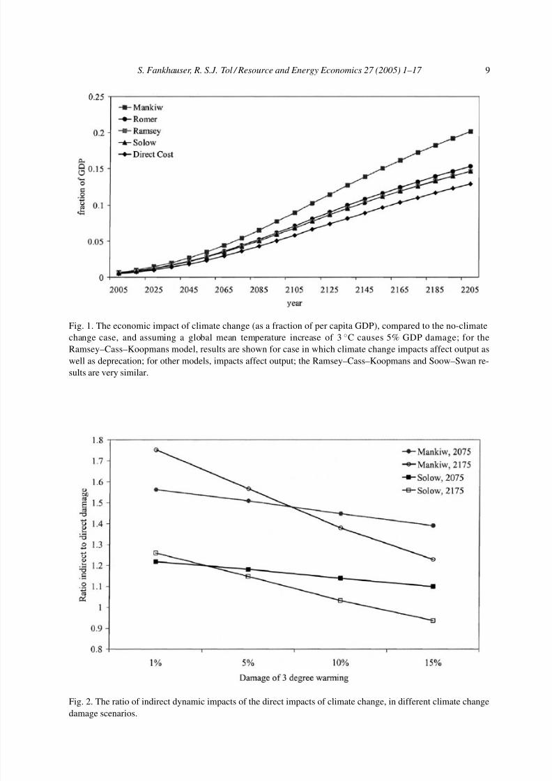
Fig. 1 compares the direct impacts of climate change with the indirect dynamic effects

for the different model specifications, using losses in per capita consumption as the damage

indicator. It also highlights the compounding nature of the dynamic effects, which growboth in absolute and relative terms over time.

The magnitude of the indirect effects differs across the models. The capital accumu-

lation effect (the difference between Solow–Swan and direct costs) is much larger than

the savings effect (the difference between Solow–Swan and the Ramsey–Cass–Koopmans

specification), which is barely distinguishable. Both are slightly bigger, in absolute terms,

than the direct losses of climate change. The dynamic effects are strongest in an endoge-

nous growth context, particularly in the Mankiw–Romer–Weil model where consumption

losses can grow to almost twice the size of direct impacts. The Romer model shows the

same effect, but smaller. This is because in these specifications a larger part of the growth is

internal to the model, rather than exogenously specified technological progress. This makes

the model more sensitive to reductions in output, and hence investments in human capital

(Mankiw–Romer–Weil) or research and development (Romer).

Fig. 2 shows the size of the dynamic effects, relative to the direct effect, for different

levels of climate change impact, ranging from 1% to 15% of GDP for 3 ◦C warming.

The comparison is limited to the Solow–Swan and the Mankiw–Romer–Weil models and

shows that the indirect effect is relatively less important for larger benchmark climate

change impacts. This is because direct impacts grow linearly with benchmark impacts

whereas investment falls inversely proportional with direct impacts, capital falls less than

proportional with investment, and output and consumption are less than linear in capital.

6 This simplification is due to Romer (1996).




Fig. 1. The economic impact of climate change (as a fraction of per capita GDP), compared to the no-climate

change case, and assuming a global mean temperature increase of 3 ◦C causes 5% GDP damage; for the

Ramsey–Cass–Koopmans model, results are shown for case in which climate change impacts affect output as

well as deprecation; for other models, impacts affect output; the Ramsey–Cass–Koopmans and Soow–Swan re-

sults are very similar.

Fig. 2. The ratio of indirect dynamic impacts of the direct impacts of climate change, in different climate change

damage scenarios.




For large impacts, indirect damages are smaller relative to direct impacts in later time

periods. In later time periods, the less-than-linear effect of benchmark damages on indirect

impacts is compounded over time. For small impacts, indirect damages are larger relative

to direct impacts in later time periods. For smaller impacts, indirect impacts are more linearin benchmark damages; in later time periods, the capital accumulation effect is larger.

The implication of this is that the static enumerative method underestimates the economic

impacts of climate change more forlow static impacts than forhigh static impacts. High static

impacts are estimated for developing countries, and low impacts for developed countries

(Smith et al., 2001). The dynamic effect thus attenuates the distributional consequences of

climate change impacts.

4. The rate of growth

We next turn to the question of how significant climate change may be for long-term

growth prospects, using the same model and model specifications as in the previous section.

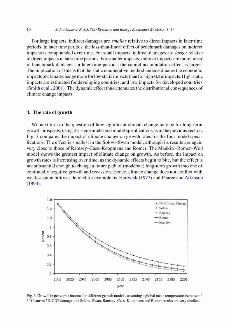
Fig. 3 compares the impact of climate change on growth rates for the four model speci-

fications. The effect is smallest in the Solow–Swan model, although its results are again

very close to those of Ramsey–Cass–Koopmans and Romer. The Mankiw–Romer–Weil

model shows the greatest impact of climate change on growth. As before, the impact on

growth rates is increasing over time, as the dynamic effects begin to bite, but the effect is

not substantial enough to change a future path of (moderate) long-term growth into one of

continually negative growth and recession. Hence, climate change does not conflict withweak sustainability as defined for example by Hartwick (1977) and Pearce and Atkinson

(1993).

Fig. 3. Growth in per capita income for different growth models, assuming a global mean temperature increase of

3 ◦C causes 5% GDP damage; the Solow–Swan, Ramsey–Cass–Koopmans and Romer results are very similar.




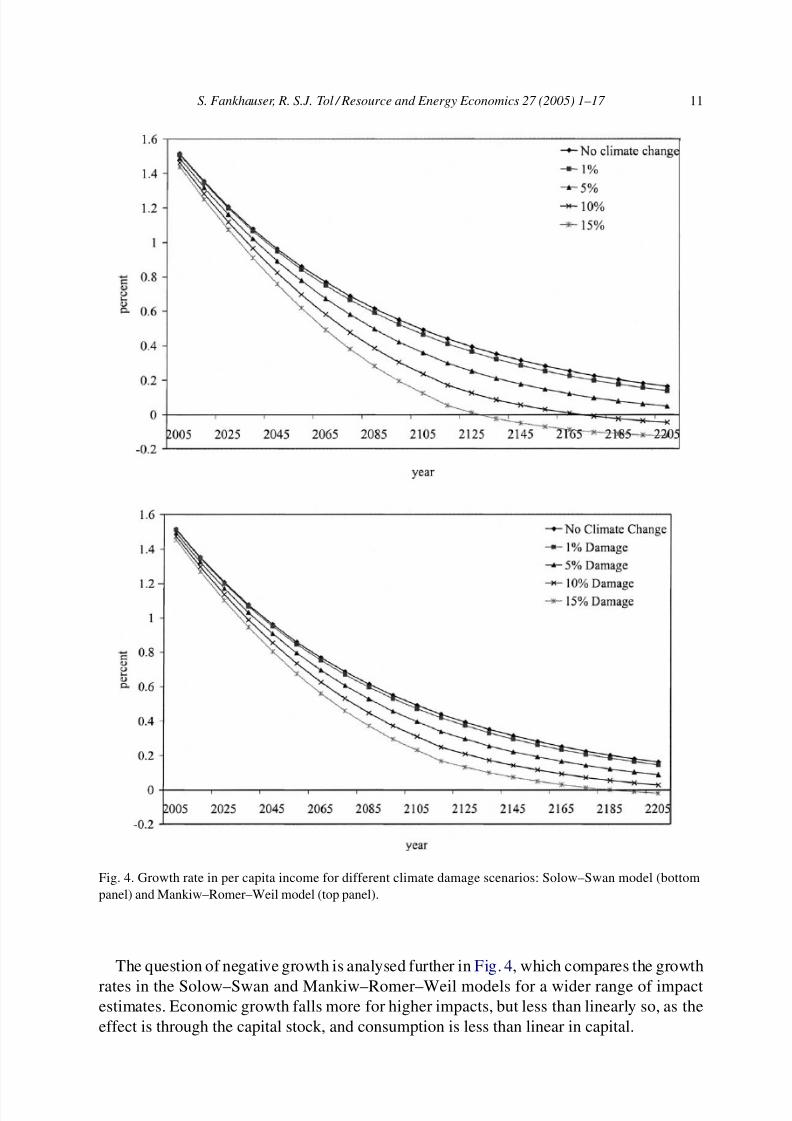
Fig. 4. Growth rate in per capita income for different climate damage scenarios: Solow–Swan model (bottom

panel) and Mankiw–Romer–Weil model (top panel).

The question of negative growth is analysed further in Fig. 4, which compares the growth

rates in the Solow–Swan and Mankiw–Romer–Weil models for a wider range of impactestimates. Economic growth falls more for higher impacts, but less than linearly so, as the

effect is through the capital stock, and consumption is less than linear in capital.






effects are most pronounced in the Mankiw–Romer–Weil specification, which includes

human capital. This model also shows the highest sensitivity to changes in impact as-

sumptions. The Solow–Swan specification with fixed savings rates is least affected by the

dynamic effects. Not surprisingly, the importance of dynamic effects grows over time,as changes in savings and investment decisions are compounded as time goes on. The

dynamic effects are also relatively larger, the smaller direct (static) impacts of climate

change.

As poorer countries are generally thought to have larger direct impacts (Smith et al.,

2001), the traditional enumerative method may underestimate the total effects most strongly

in developed countries. This is further pronounced if we consider that countries with

different levels of income have different growth mechanisms. In very poor countries,

physical capital accumulation is most important. If countries grow richer, human capi-

tal accumulation becomes more important, and in fully developed economies, knowledge

accumulation becomes more important (Funke and Strulik, 2000). The Solow–Swan and

Ramsey–Cass–Koopmans models emphasize physical capital accumulation, and are less

sensitive to climate change. The Mankiw–Romer–Weil and Romer models emphasize hu-

man capital and knowledge accumulation, respectively, and are more sensitive to climate

change.

This paper is only a first step toward a better understanding of the links between cli-

mate change and economic growth. Many questions remain and we need to bear in mind

the limitations of the modeling approach we have chosen. First, the savings and capi-

tal accumulation effects discussed in this paper are not the only channels through which

climate change may affect growth. Scheraga et al. (1993) have pointed out the effect cli-mate change may have on the structure of economies. As a result of climate change some

sectors will grow faster than others, thereby changing the size and composition of GDP.

In addition, the demand for defensive investments, such as sea walls, may well grow at

the expense of other investments. Arguably, such changes in the structure of an economy

could have an impact on its long-term growth potential. Similarly, the model we use is

one of a closed economy, and international trade may well exacerbate negative impacts

in one place and alleviate impacts somewhere else (Darwin and Tol, 2001). Similarly,

countries are linked through international capital flows. Climate change would affect the

supply of capital (through its effect on income) as well as the relative rates of return on

investment.By choosing standard growth models, we have overlooked the powerful lessons that the

‘new economic geography’ literature has taught us about the importance of climate and

disease as a determinant of long-term economic development. Gallup et al. (1999) argue

that vector-borne diseases, particularly malaria, can have such a large effect on labour

productivity that some countries, particularly in Sub-Saharan Africa are trapped in a vicious

cycle of disease–low productivity–poverty–deficient health care. Climate change may well

lead to an increase in vector-borne diseases, which could make more countries vulnerable

to this poverty–disease trap. For instance, Gallup et al. (1999) find that malaria slows

economic growth in Africa by about 1% per year, while McMichael et al. (1996) find that

a degree of global warming may increase malaria by some 10%. Masters and McMillan(2001) find a clear positive relationship between mild frost and economic development. They

speculate that frost kills pests and pathogens, so that human and agricultural productivity is




higher in temperate climates. Again, climate change may reduce this advantage.7 However,

Acemoglu et al. (2001) argue for a much weaker and much more indirect influence of

climate on development.

A final comment has to concern the ethical underpinnings of the model we have chosen.The objective of our model was to maximize aggregate social welfare, expressed as the

present value of utility achieved over time. This representation is typical for growth models,

but it may not be an appropriate objective for climate change policy, or should at least not

be its only goal. Indeed, an economic response to climate change that reduces saving and

shifts consumption from the future to the present falls foul of a key goal of climate change

policy: intergenerational equity. However, broadening the approach to include a wider set

of social objectives will have to be left to future research.

Acknowledgements

Thanks to our friend and colleague Joel Smith for asking the question that led us to

writing this paper. Kerstin Ronneberger, Charles Kolstad and an anonymous referee pro-

vided valuable comments on an earlier draft. The Volkswagen Foundation through the

ECOBICE project, the US National Science Foundation through the Center for Integrated

Study of the Human Dimensions of Global Change (SBR-9521914) and the Michael Otto

Foundation provided welcome financial support. The views expressed in this paper are the

authors’ and not necessarily those of the organisations they are affiliated with. All errors are

ours.

Appendix A. Growth models

The numerical models used in Sections 3 and 4 are based on DICE (Nordhaus, 1994),

but use the specifications for output and capital accumulation discussed below. Initial con-

ditions, parameters and scenarios (labour, productivity) are taken from Nordhaus (1994).

Nordhaus uses a Ramsey–Cass–Koopmans model. The other three models are calibrated

such that, in the absence of climate change, production and consumption are equal in all

time periods to the Ramsey–Cass–Koopmans model. The main calibration parameter is

productivity. Parameters are chosen such that, in the absence of climate change, models

converge to a balanced growth path.

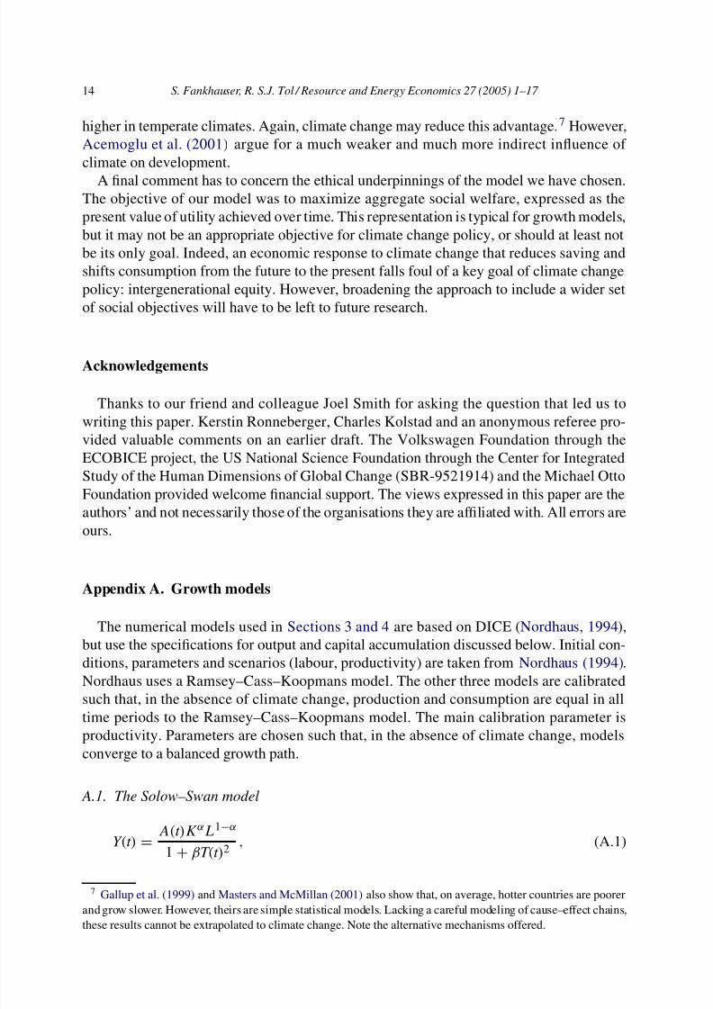
A.1. The Solow–Swan model

Y(t) =A(t)KαL1−α

1 + βT(t)2, (A.1)

7 Gallup et al. (1999) and Masters and McMillan (2001) also show that, on average, hotter countries are poorer

and grow slower. However, theirs are simple statistical models. Lacking a careful modeling of cause–effect chains,

these results cannot be extrapolated to climate change. Note the alternative mechanisms offered.




where Y is the output, A the productivity, K the physical capital, L the labour, T the temper-

ature, t the time and α = 0.25; β = 0.05/9 for the base case.

˙K = s(t)Y(t) − δK(t), (A.2)

where s is the savings’ rate and δ = 0.1 the depreciation rate. The savings rate s is at each

point in time set equal to the savings rate of the Ramsey–Cass–Koopmans model without

climate change impacts; it gradually falls from 19% at present to 16% in 2300.

A.2. The Ramsey–Cass–Koopmans model

The Ramsey–Cass–Koopmans model is identical to the Solow–Swan model, except that

the savings rate is determined by intertemporal optimization. For this, we used the DICE

model of Nordhaus (1994) as implemented in GAMS. We also took productivity, labourand the initial capital stock from DICE.

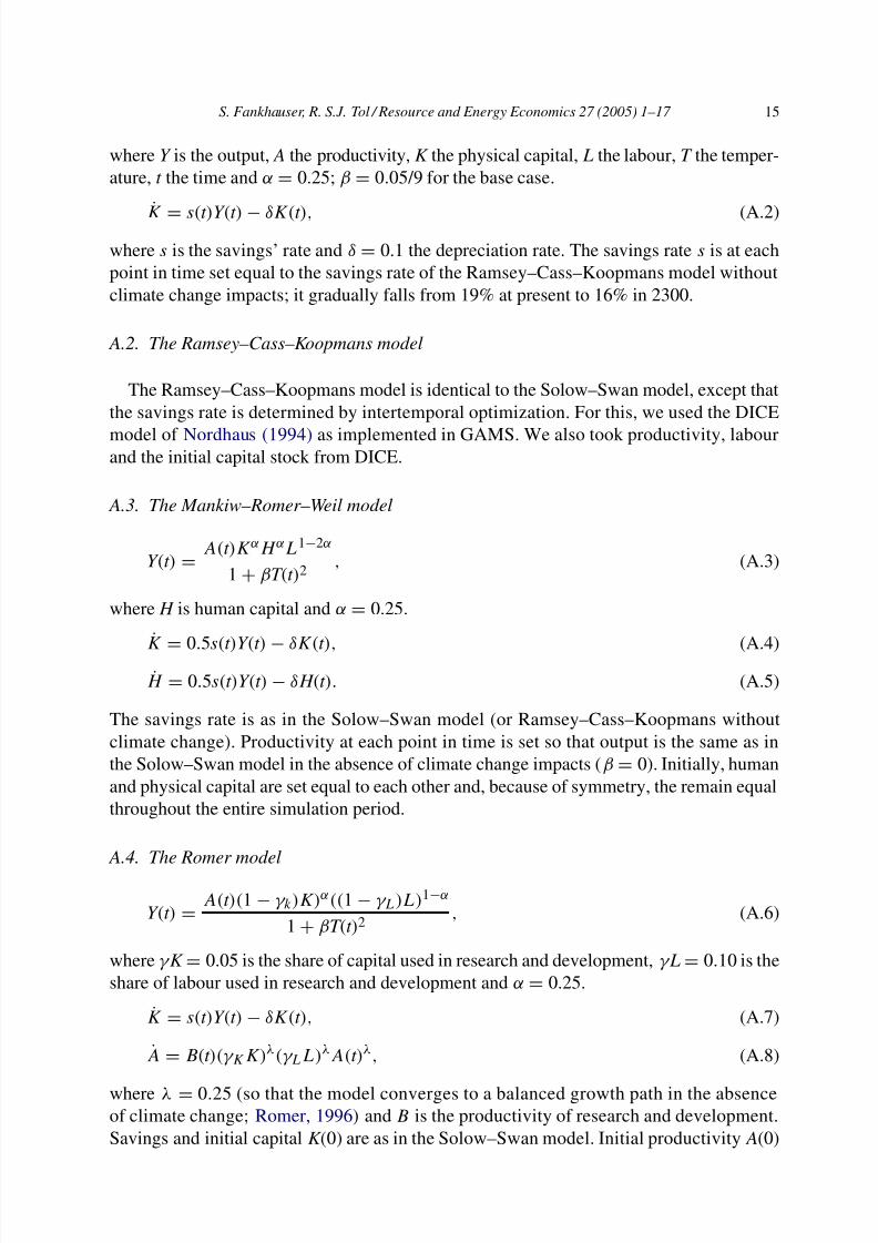
A.3. The Mankiw–Romer–Weil model

Y(t) =A(t)KαH αL1−2α

1 + βT(t)2, (A.3)

where H is human capital and α = 0.25.

K = 0.5s(t)Y(t) − δK(t), (A.4)

H = 0.5s(t)Y(t) − δH(t). (A.5)

The savings rate is as in the Solow–Swan model (or Ramsey–Cass–Koopmans without

climate change). Productivity at each point in time is set so that output is the same as in

the Solow–Swan model in the absence of climate change impacts (β = 0). Initially, human

and physical capital are set equal to each other and, because of symmetry, the remain equal

throughout the entire simulation period.

A.4. The Romer model

Y(t) =A(t)(1 − γ k)K)α((1 − γ L)L)1−α

1 + βT(t)2, (A.6)

where γ K = 0.05 is the share of capital used in research and development, γ L = 0.10 is the

share of labour used in research and development and α = 0.25.

K = s(t)Y(t) − δK(t), (A.7)

A = B(t)(γ KK)λ(γ LL)λA(t)λ, (A.8)

where λ = 0.25 (so that the model converges to a balanced growth path in the absenceof climate change; Romer, 1996) and B is the productivity of research and development.

Savings and initial capital K (0) are as in the Solow–Swan model. Initial productivity A(0)




and R&D productivity B(t ) are set so that in each period output is the same as in the

Solow–Swan model in the absence of climate change impacts (β = 0).

References

Acemoglu, D., Johnson, S., Robinson, J.A., 2001. The colonial origins of comparative development: an empirical

investigation. American Economic Review 91, 1369–1401.

Aghion, P., Howitt, P., 1992. A model of growth through creative destruction. Econometrica 56, 323–351.

Barro, R.J., Sala-I-Martin, X., 1995. Economic Growth. McGraw-Hill, New York.

Cline, W.R., 1992. The Economics of Global Warming. Institute for International Economics, Washington, DC.

Cline, W.R., 1994. The costs and benefits of greenhouse gas abatement. A guide to policy analysis. In: OECD

(Ed.), The Economics of Climate Change. OECD, Paris.

Darwin, R.F., Tol, R.S.J., 2001. Estimates of the economic effects of sea level rise. Environmental and Resource

Economics 19 (2), 113–129.Fankhauser, S., 1995. Valuing Climate Change. The Economics of the Greenhouse. Earthscan, London.

Fankhauser, S., Smith, J.B., Tol, R.S.J., 1999. Weathering climate change. Some simple rules to guide adaptation

investments. Ecological Economics 30 (1), 67–78.

Funke, M., Strulik, H., 2000. On endogenous growth with physical capital, human capital and product variety.

European Economic Review 44, 491–515.

Gallup, J.L., Sachs, J.D., Mellinger, A., 1999. Geography and Economic Development, CID Working Paper 1.

Harvard Center for International Development, Cambridge.

Grossman, G.M., Helpman, E., 1991. Innovation and Growth in the Global Economy. MIT Press, Cambridge.

Hartwick, J.M., 1977. Intergenerational equity and the investing of rents from exhaustible resources. American

Economic Review 67 (5), 972–974.

Mankiw, N.G., Romer, D., Weil, D.N., 1992. A contribution to the empirics of economic growth. Quarterly Journalof Economics 107 (2), 407–437.

Masters, W.A., McMillan, M.S., 2001. Climate and scale in economic growth. Journal of Economic Growth 6,

167–186.

McMichael, A.J., Ando, M., Carcavallo, R., Epstein, P., Haines, A., Jendritzky, G., Kalkstein, L., Odongo, R.,

Patz, J., Piver, W., 1996. Human population health. In: IPCC (Ed.), Climate Change 1995: Impact, Adaptation

and Mitigation of Climate Change: Scientific-Technical Analysis—Contribution of Working Group II to the

Second Assessment Report of the Intergovernmental Panel on Climate Change. Cambridge University Press,

Cambridge.

McMichael, A., Githeko, A., Akhtar, R., Carcavallo, R., Gubler, D., Haines, D., Kovats, R.S., Martens, P., Patz, J.,

Sasaki, A., 2001. Human health. In: IPCC (Ed.), Climate Change 2001: Impacts, Adaptation and Vulnerability.

Contribution of Working Group II to the Third Assessment Report. Cambridge University Press, Cambridge.

Mendelsohn, R.O., Neumann, J.E. (Eds.), 1999. The Impact of Climate Change on the United States Economy.Cambridge University Press, Cambridge.

Nordhaus, W.D., 1991. To slow or not to slow: the economics of the greenhouse effect. Economic Journal 101,

920–937.

Nordhaus, W.D., 1994. Managing the Global Commons: the Economics of Climate Change. The MIT Press,

Cambridge.

Pearce, D.W., Atkinson, G., 1993. Capital theory and the measurement of sustainable development: an indicator

of ‘weak’ sustainability. Ecological Economics 8, 103–108.

Peck, S.C., Teisberg, T.J., 1992. CETA: a model for carbon emissions trajectory assessment. Energy Journal 13 (1),

55–77.

Romer, P.M., 1990. Endogenous technological change. Journal of Political Economy 98, S71–S102.

Romer, D., 1996. Advanced Macroeconomics. McGraw-Hill, New York.Scheraga, J.D., Learly, N.A., Goettle, R.J., Jorgenson, D.W., Wilkoxen, P.J., 1993. Macroeconomic modelling and

the assessment of climate change impacts. In: Kaya, Y., Nakicenovic, N., Nordhaus, W., Toth, F. (Eds.), Costs,

Impacts and Benefits of CO2 Mitigation. IIASA, Laxenburg.




Smith, J.B., Schellnhuber, H.-J., Mirza, M.Q., Lin, E., Fankhauser, S., Leemans, R., Ogallo, L., Richels, R.G.,

Safriel, U., Tol, R.S.J., Weyant, J.P., Yohe, G.W., 2001. Vulnerability to climate change and reasons for concern:

a synthesis. In: IPCC (Ed.), Climate Change 2001: Impacts, Adaptation and Vulnerability. Contribution of

Working Group II to the Third Assessment Report. Cambridge University Press, Cambridge.Tol, R.S.J., 1995. The damage costs of climate change toward more comprehensive calculations. Environmental

and Resource Economics 5, 353–374.

Tol, R.S.J., 1999. The marginal damage costs of greenhouse gas emissions. The Energy Journal 20 (1), 61–81.

Tol, R.S.J., Fankhauser, S., Richels, R.G., Smith, J.B., 2000. How much damage will climate change do? Recent

Estimates. World Economics 1 (4), 179–206.

Documents

Cambio Climatico Ramsey