Embed Size (px)
Citation preview
HAL Id: tel-00403501https://tel.archives-ouvertes.fr/tel-00403501
Submitted on 10 Jul 2009
HAL is a multi-disciplinary open accessarchive for the deposit and dissemination of sci-entific research documents, whether they are pub-lished or not. The documents may come fromteaching and research institutions in France orabroad, or from public or private research centers.
L’archive ouverte pluridisciplinaire HAL, estdestinée au dépôt et à la diffusion de documentsscientifiques de niveau recherche, publiés ou non,émanant des établissements d’enseignement et derecherche français ou étrangers, des laboratoirespublics ou privés.
Caractérisation des réservoirs pétroliers par les donnéessismiques, avec l’aide de la géomodélisation
Audrey Neau
To cite this version:Audrey Neau. Caractérisation des réservoirs pétroliers par les données sismiques, avec l’aide de lagéomodélisation. Géophysique [physics.geo-ph]. Université de Pau et des Pays de l’Adour, 2009.Français. <tel-00403501>
Numéro d'attribution à la bibliothèque|_|_|_|_|_|_|_|_|_|_|
THÈSE
Présentée à
L'Université de Pau et des Pays de l'AdourEcole doctorale
� Sciences exactes et leurs applications �
Par
Audrey NEAU
Pour obtenir le grade de
Docteur
Spécialité : Exploration géophysique
Caractérisation des réservoirspétroliers par les données sismiques,avec l'aide de la géomodélisation
soutenue publiquement le 14 mai 2009 devant le jury composé de
Béatrice de Voogd Université de Pau et des Pays de l'Adour Directeur de thèsePierre Thore TOTAL SA, Pau Co-Directeur de thèseHervé Perroud Université de Pau et des Pays de l'Adour Président du juryJean-Paul Chilès Ecole des Mines de Paris RapporteurFrédérique Fournier Beicip Franlab, Rueil Malmaison RapporteurPhilippe Doyen CGGVeritas, Crawley UK ExaminateurMrinal K. Sen Université du Texas, Austin USA Examinateur
Département Innovation du C.S.T.J.F. de TOTALLaboratoire de Modélisation et Imagerie en Géosciences (MIGP) - UMR 5212 - Pau


i
"Gloire à toi, Archimède, qui fut le premier à démon-trer que, lorsque l'on plonge un corps dans une bai-gnoire, le téléphone sonne."Pierre DESPROGES
"Dans les sciences, le chemin est plus important que lebut. Les sciences n'ont pas de �n."Erwin CHARGAFF

ii
Remerciements
Ce manuscrit rassemble l'ensemble du travail scienti�que de trois années de thèse. Maisune thèse ne se résume pas simplement aux résultats scienti�ques, ce sont également desrencontres, une expérience humaine et donc un enrichissement personnel de trois ans d'unevie, ponctués de bons moments et d'obstacles à surmonter.Ces trois années bien remplies, qui sont une part de vie et que je n'oublierai pas, je lesdois à tous les échanges scienti�ques, à toutes les personnes qui m'ont encouragées etsoutenues, et en�n à toutes les personnes que j'ai croisées pendant cette � parenthèse �de ma vie. Cette page de remerciement leur est destinée, et j'espère n'oublier personne.Si c'est le cas, mille excuses : il y a peut-être des oublis sur le papier, mais pas dans l'esprit !
Je tiens tout d'abord à remercier l'instigateur de cette thèse et co-directeur, MonsieurPierre Thore, pour avoir cru en moi et m'avoir lancée dans cette aventure, en me permet-tant de faire ce travail dans les meilleures conditions possibles, pour m'avoir d'abord guidéepas à pas puis laissée voler de mes propres ailes.
Mes remerciements vont également à ma directrice, Madame Béatrice De Voogd, poursa présence e�cace tout au long de la thèse, pour sa disponibilité, sa réactivité et ses com-pétences. Merci pour toujours avoir valorisé mon travail et m'avoir donnée plus con�anceen moi.
Madame Frédérique Fournier et Monsieur Jean-Paul Chilès ont accepté d'être les rap-porteurs de cette thèse, et je les en remercie. Ils ont également contribué par leurs nom-breuses remarques et suggestions à améliorer la qualité de ce mémoire, et je leur en suistrès reconnaissante.
Messieurs Philippe Doyen, Hervé Perroud et Mrinal Sen m'ont fait l'honneur de parti-ciper au Jury de soutenance ; je les en remercie profondément. Remerciements particuliersà Monsieur Hervé Perroud pour avoir accepté le rôle de président du jury de cette thèse,la première issue de son projet de Master.
Je remercie Messieurs Jérôme Guilbot et Ramin Nawab, successivement chefs du dépar-tement Innovation de Total, pour m'avoir accueillie dans leur équipe, et pour les conseilsstimulants que j'ai eu l'honneur de recevoir de leurs parts. Merci à tous les membres ac-tuels et passés de cette entité, Jean-Luc, Hassan, Feï, Juan, Frédéric, Anthony, Maryvonne,Francis, Sung, Didier, Ehsan, pour m'avoir intégrée dans le service non pas comme une sta-giaire mais avec autant d'égard qu'une collègue.
Je ne saurais jamais assez remercier Issam Tarrass pour sa bonne humeur quotidienne,pour son soutien moral permanent et pour sa gentillesse. J'ai eu la chance de partager son

iv Remerciements
bureau pendant trois ans... un véritable ami à présent. Un grand merci à toi. Et un grosM.... pour la �n de ta thèse !
Je remercie tous ceux sans qui cette thèse ne serait pas ce qu'elle est : aussi bien parles discussions que j'ai eu la chance d'avoir avec eux, leurs suggestions ou contributions.Je pense ici en particulier à Messieurs Marc Elias et Eric Maocec pour le champ Alpha,à Lorette Anquelle, Yoann Guilloux et Dimitri Modin pour le champ Bêta, et à CécilePabian, Jean Luc Broyer, Alain Jegoux et Matthieu Pellerin pour le champ Gamma. Merciaux collègues de CGGVeritas, Rémi, Raphael, Robert pour leur aide sur GeoSI. Je remercieégalement Messieurs Jean Luc Piazza, Emmanuel Chavanne, Pierre Biver, et Léon Barenspour les discussions et suggestions en géomodélisation. Un grand merci à Benoit Paternos-ter pour ces discussions où l'on vient avec une question et dont on ressort la tête pleine denouveaux horizons...
En ce qui concerne la partie informatique de ce travail, je remercie Messieurs GuillaumeMorin et Sylvain Sangla pour leur aide précieuse en programmation, ainsi que l'équipesupport de Sismage, David, Rabah, Khalid pour leur volonté de toujours répondre à mesquestions. Frédéric Mansanné et Sylvain Toinet ont été très présents lors de l'implémenta-tion informatique de mes travaux, et je les en remercie énormément.
Je passe ensuite une dédicace spéciale à tous les jeunes gens que j'ai eu le plaisir decôtoyer durant ces quelques années à Pau, je pense notamment à Alain-Christophe, Ma-thieu, Livinus, Maelle, Khalil, Ravi, Paritosh, Désirée, Céline, et tous les étudiants despromotions 2008 et 2009 du Master Génie Pétrolier de Pau, à qui j'ai dispensés quelquescours de caractérisation réservoir.
Je souhaite également remercier Jean Claude Mercier, mon ancien Professeur de LaRochelle, pour avoir fait le trajet jusqu'à Pau rien que pour assister à ma soutenance.Quelle belle surprise vous m'avez faite !
Mes remerciements vont également vers François Levêque pour m'avoir lancée sur cettevoie, pour avoir cru en ma motivation et pour s'être décarcassé pour que je puisse assisterà tous les camps de terrain. Je ne saurai jamais assez remercier Guy Sénéchal pour sesencouragements précieux qui m'ont permis de garder la tête hors de l'eau quand les chosesétaient di�ciles en Licence et pour avoir partagé le projet Rustrel avec moi deux annéesde suite.
En�n, mais pas des moindres, un grand merci à mes amis, mes trois petits rayons desoleil, Florence, Aurélie et Julia. Et aussi à Vicky pour m'avoir supporté au quotidien, dansles moments di�ciles. Un grand merci à Anne et Bernard pour m'avoir "adoptée" et pouravoir été présents à tout instant. Petit clin d'oeil à Annick et Nicole pour avoir suivi monparcours et pour votre présence le jour J.
Ces remerciements ne sauraient être complets si ma famille n'était citée. J'ai gardé lemeilleur pour la �n : un grand merci à toute ma famille qui m'a toujours fait con�anceet soutenue dans mes choix. Tout au long de mes études, vous avez su m'encourager etme remonter le moral dans les moments di�ciles, et m'avez permis de réaliser mes projets...
A tous, merci.

Remerciements v
À ma grand-mère Elise qui n'a pas pu voirl'aboutissement de ce travail.

Caractérisation des réservoirs pétroliers par lesdonnées sismiques avec l'aide de la géomodélisation
Résumé :La caractérisation sismique des réservoirs pétroliers nécessite l'intégration de plusieurstechniques telles que la lithosismique, la géomodélisation, la géostatistique, l'utilisationdes algorithmes évolutionnaires et la pétrophysique. L'information sismique est d'abordutilisée pour la description de l'architecture externe des réservoirs car son utilisation pourla description des faciès ne se fait pas sans di�cultés. L'objectif de cette thèse est d'appor-ter des outils nouveaux pour aider à l'utilisation de l'information sismique pour caractériserles réservoirs.Un premier travail a consisté à évaluer l'impact des incertitudes structurales sur les inver-sions pétroélastiques et les conséquences en terme de classi�cation de faciès. Ensuite, nousconsidérons la modélisation sismique comme aide à l'évaluation du modèle réservoir. Cettemodélisation permettra de faire le lien entre les simulateurs réservoir ou les géomodeleurset la réponse sismique du réservoir.Nous développons ensuite deux approches alternatives aux méthodes traditionnelles en in-version pétroélastique et pétrophysique. La première utilise la méthode géostatistique desdéformations graduelles pour créer des réalisations de propriétés réservoirs. Elle permetde créer des propriétés à l'échelle réservoir, conditionnées aux puits, tout en respectantune fonction coût basée sur la comparaison des données sismiques réelles et issues de cesréalisations.La seconde méthode repose sur le principe de la classi�cation supervisée et utilise des ré-seaux de neurones pour analyser la forme des traces sismiques. Une première étape consisteà générer un volume d'apprentissage contenant tous les modèles pétrophysiques envisa-geables pour un champ donné. Ces modèles sont analysés par les réseaux de neurones. Lesneurones ainsi identi�és sont appliqués aux données réelles, pour identi�er des relationspétrophysique/sismique identiques aux données d'apprentissage.Toutes les méthodologies sont validées sur plusieurs réservoirs choisis pour leurs particula-rités géologiques (complexité structurale, lithologie du réservoir).
Mots-clés : Caractérisation réservoir, sismique, inversion, géomodélisation, interprétation,réseaux de neurones.
vii
Reservoir characterization based on seismic data withthe help of geomodeling methods
Abstract :Seismic characterization of hydrocarbon reservoirs is based on various techniques : litho-seismic, geomodeling, geostatistics, evolutionary algorithms, and petrophysics. Seismic in-formation is �rst used for the description of the reservoir structure, but then its relationshipwith facies description is a di�cult task. The aim of this thesis is to develop new tools forseismic reservoir characterization.A �rst work has consisted in evaluating the impact of structural uncertainties on petroe-lastic inversion and its consequences in terms of facies classi�cation. Then, we considerseismic modeling as an aid to reservoir model evaluation. This modeling step will make theconnection between the reservoir simulators (or geomodelers) and the seismic response ofthe reservoir.Then we develop two alternative approaches for petroelastic and petrophysical inversion.The �rst one uses the gradual deformation method to generate reservoir property realiza-tions. This method generates properties at the reservoir scale, conditioned by the wells,while respecting a cost function based on the comparison of actual and synthetic seismicdata.The second method is based on supervised classi�cation principle and uses neural networksto analyze the waveform of seismic traces. A �rst step is to generate a volume containingall possible petrophysical models for the concerned �eld. These models are analyzed by theneural networks. The neurons identi�ed are applied on the actual data to recognize similarpetrophysical/seismic relationships.All methods are tested and validated on actual reservoirs, chosen for their speci�c features(structural complexity, reservoir lithology).
Keywords : Reservoir characterization, seismic, inversion, geomodeling, interpretation, neu-ral networks.
Table des matières
Remerciements iiiRésumé viAbstract viiListe des �gures xixListe des tableaux xx1 Introduction générale 1
1.1 Problématique . . . . . . . . . . . . . . . . . . . . . . . . . . . . . . . . . . 11.2 Contexte scienti�que . . . . . . . . . . . . . . . . . . . . . . . . . . . . . . . 3
1.2.1 L'ingénierie du réservoir pétrolier . . . . . . . . . . . . . . . . . . . . 41.2.2 Les propriétés réservoirs . . . . . . . . . . . . . . . . . . . . . . . . . 8
1.3 Organisation de la thèse . . . . . . . . . . . . . . . . . . . . . . . . . . . . . 112 Présentation des données utilisées 15
2.1 Introduction . . . . . . . . . . . . . . . . . . . . . . . . . . . . . . . . . . . . 152.2 Avant-propos sur les données sismiques . . . . . . . . . . . . . . . . . . . . . 15
2.2.1 Caractéristiques des ondes et propriétés des roches . . . . . . . . . . 152.2.2 Acquisition et traitement . . . . . . . . . . . . . . . . . . . . . . . . 18
2.3 Le champ Alpha - modèle turbiditique . . . . . . . . . . . . . . . . . . . . . 212.3.1 Le contexte géologique . . . . . . . . . . . . . . . . . . . . . . . . . . 212.3.2 Le modèle réservoir . . . . . . . . . . . . . . . . . . . . . . . . . . . . 242.3.3 Les données sismiques . . . . . . . . . . . . . . . . . . . . . . . . . . 272.3.4 Les particularités du champ Alpha . . . . . . . . . . . . . . . . . . . 29
2.4 Le champ Bêta - modèle turbiditique . . . . . . . . . . . . . . . . . . . . . . 302.4.1 Le contexte géologique . . . . . . . . . . . . . . . . . . . . . . . . . . 302.4.2 Le modèle réservoir . . . . . . . . . . . . . . . . . . . . . . . . . . . . 322.4.3 Les données puits . . . . . . . . . . . . . . . . . . . . . . . . . . . . . 332.4.4 Les données sismiques . . . . . . . . . . . . . . . . . . . . . . . . . . 362.4.5 Les particularités du champ Bêta . . . . . . . . . . . . . . . . . . . . 38
2.5 Le champ Gamma - modèle carbonaté . . . . . . . . . . . . . . . . . . . . . 392.5.1 Le contexte géologique . . . . . . . . . . . . . . . . . . . . . . . . . . 392.5.2 Les particularités du champ Gamma . . . . . . . . . . . . . . . . . . 40
I - Validité de la grille réservoir 433 Modélisation sismique à partir de la grille réservoir 43
Table des matières ix
3.1 Introduction . . . . . . . . . . . . . . . . . . . . . . . . . . . . . . . . . . . . 433.2 Calcul des données sismiques synthétiques . . . . . . . . . . . . . . . . . . . 44
3.2.1 Le modèle convolutionnel 1D . . . . . . . . . . . . . . . . . . . . . . 443.2.2 Le tracé de rayons . . . . . . . . . . . . . . . . . . . . . . . . . . . . 453.2.3 Modélisation numérique de l'équation des ondes . . . . . . . . . . . . 45
3.3 Transformation en grille régulière . . . . . . . . . . . . . . . . . . . . . . . . 463.4 Evaluation des modélisations sur le champ Alpha . . . . . . . . . . . . . . . 48
3.4.1 E�ets du changement de support Sismique-Réservoir-Voxet . . . . . 483.4.2 Sismogrammes synthétiques 1D . . . . . . . . . . . . . . . . . . . . . 503.4.3 Modélisation sismique à partir d'une grille réservoir . . . . . . . . . . 51
3.5 Lissage des propriétés du voxet . . . . . . . . . . . . . . . . . . . . . . . . . 533.6 Comparaison des sismiques réelles et synthétiques . . . . . . . . . . . . . . . 553.7 Conclusions et perspectives . . . . . . . . . . . . . . . . . . . . . . . . . . . 59
4 L'impact des incertitudes structurales 614.1 Introduction . . . . . . . . . . . . . . . . . . . . . . . . . . . . . . . . . . . . 624.2 Multiple reservoir grid realizations . . . . . . . . . . . . . . . . . . . . . . . 62
4.2.1 Probability Fields method . . . . . . . . . . . . . . . . . . . . . . . . 634.2.2 Uncertainty representation . . . . . . . . . . . . . . . . . . . . . . . . 644.2.3 Application on Alpha �eld . . . . . . . . . . . . . . . . . . . . . . . . 65
4.3 Stochastic inversion . . . . . . . . . . . . . . . . . . . . . . . . . . . . . . . . 694.3.1 GeoSI operating principles . . . . . . . . . . . . . . . . . . . . . . . . 704.3.2 Prior model building . . . . . . . . . . . . . . . . . . . . . . . . . . . 704.3.3 Generation and QC of seismic attributes . . . . . . . . . . . . . . . . 72
4.4 Facies classi�cation . . . . . . . . . . . . . . . . . . . . . . . . . . . . . . . . 744.4.1 Well log scale . . . . . . . . . . . . . . . . . . . . . . . . . . . . . . . 764.4.2 Seismic scale . . . . . . . . . . . . . . . . . . . . . . . . . . . . . . . 784.4.3 Probabilistic facies cubes . . . . . . . . . . . . . . . . . . . . . . . . 80
4.5 Facies repartition in the reservoir grid . . . . . . . . . . . . . . . . . . . . . 804.5.1 Upscaling at the reservoir grid scale . . . . . . . . . . . . . . . . . . 804.5.2 Comparison of facies repartition in each model . . . . . . . . . . . . 84
4.6 Conclusion . . . . . . . . . . . . . . . . . . . . . . . . . . . . . . . . . . . . . 87
II - Alternatives à l'approche directe 915 Inversion par déformation graduelle 91
5.1 Introduction . . . . . . . . . . . . . . . . . . . . . . . . . . . . . . . . . . . . 915.2 Principe de fonctionnement des déformations graduelles . . . . . . . . . . . 92
5.2.1 Formulation de base . . . . . . . . . . . . . . . . . . . . . . . . . . . 935.2.2 Génération des réalisations secondaires . . . . . . . . . . . . . . . . . 945.2.3 Conditionnement aux données de puits . . . . . . . . . . . . . . . . . 96
5.3 Optimisation et itération du processus . . . . . . . . . . . . . . . . . . . . . 975.3.1 Optimisation dans l'espace de recherche . . . . . . . . . . . . . . . . 975.3.2 Données sismiques synthétiques et comparaison aux données réelles . 995.3.3 Itération . . . . . . . . . . . . . . . . . . . . . . . . . . . . . . . . . . 100
5.4 Application sur le champ Alpha . . . . . . . . . . . . . . . . . . . . . . . . . 1005.4.1 Le modèle initial . . . . . . . . . . . . . . . . . . . . . . . . . . . . . 1015.4.2 Le modèle réel . . . . . . . . . . . . . . . . . . . . . . . . . . . . . . 1045.4.3 Paramètrisation de l'inversion par déformations graduelles . . . . . . 104
x Table des matières
5.4.4 Analyse des résultats . . . . . . . . . . . . . . . . . . . . . . . . . . . 1075.4.5 In�uence du variogramme . . . . . . . . . . . . . . . . . . . . . . . . 1115.4.6 Données sismiques réelles versus données sismiques "solution" . . . . 114
5.5 Conclusions et perspectives . . . . . . . . . . . . . . . . . . . . . . . . . . . 1166 Petrophysical inversion by neural supervised classi�cation 117
6.1 Introduction . . . . . . . . . . . . . . . . . . . . . . . . . . . . . . . . . . . . 1176.2 The methodology . . . . . . . . . . . . . . . . . . . . . . . . . . . . . . . . . 1186.3 Neural Networks : Kohonen Self-Organizing Maps . . . . . . . . . . . . . . . 1206.4 Data preparation for the Beta �eld . . . . . . . . . . . . . . . . . . . . . . . 124
6.4.1 Well log preparation . . . . . . . . . . . . . . . . . . . . . . . . . . . 1246.4.2 Preliminary tests . . . . . . . . . . . . . . . . . . . . . . . . . . . . . 129
6.5 Neural Network classi�cation applied to Beta �eld . . . . . . . . . . . . . . 1336.5.1 Training from petrophysical models . . . . . . . . . . . . . . . . . . . 1336.5.2 Training from seismic data . . . . . . . . . . . . . . . . . . . . . . . . 1386.5.3 Validation and interpretation of results . . . . . . . . . . . . . . . . . 142
6.6 Data Preparation for the Gamma Field . . . . . . . . . . . . . . . . . . . . . 1456.6.1 Well log preparation . . . . . . . . . . . . . . . . . . . . . . . . . . . 1456.6.2 Neural Network classi�cation . . . . . . . . . . . . . . . . . . . . . . 1486.6.3 Preliminary tests . . . . . . . . . . . . . . . . . . . . . . . . . . . . . 148
6.7 Neural network classi�cation applied to Gamma �eld . . . . . . . . . . . . . 1516.7.1 Training from petrophysical models . . . . . . . . . . . . . . . . . . . 1516.7.2 Training from seismic data . . . . . . . . . . . . . . . . . . . . . . . . 1556.7.3 Validation and interpretation of results . . . . . . . . . . . . . . . . . 160
6.8 Concluding remarks and perspectives . . . . . . . . . . . . . . . . . . . . . . 163
III - Conclusions et perspectives 167Concluding remarks and future research 167
Annexes 173Annexe 1 : SEG Annual Conference (San Antonio 2007) 173Annexe 2 : EAGE Annual Conference (Rome 2008) 179Annexe 3 : SEG Annual Conference (Las Vegas 2008) 185
Bibliographie 193
Table des �gures
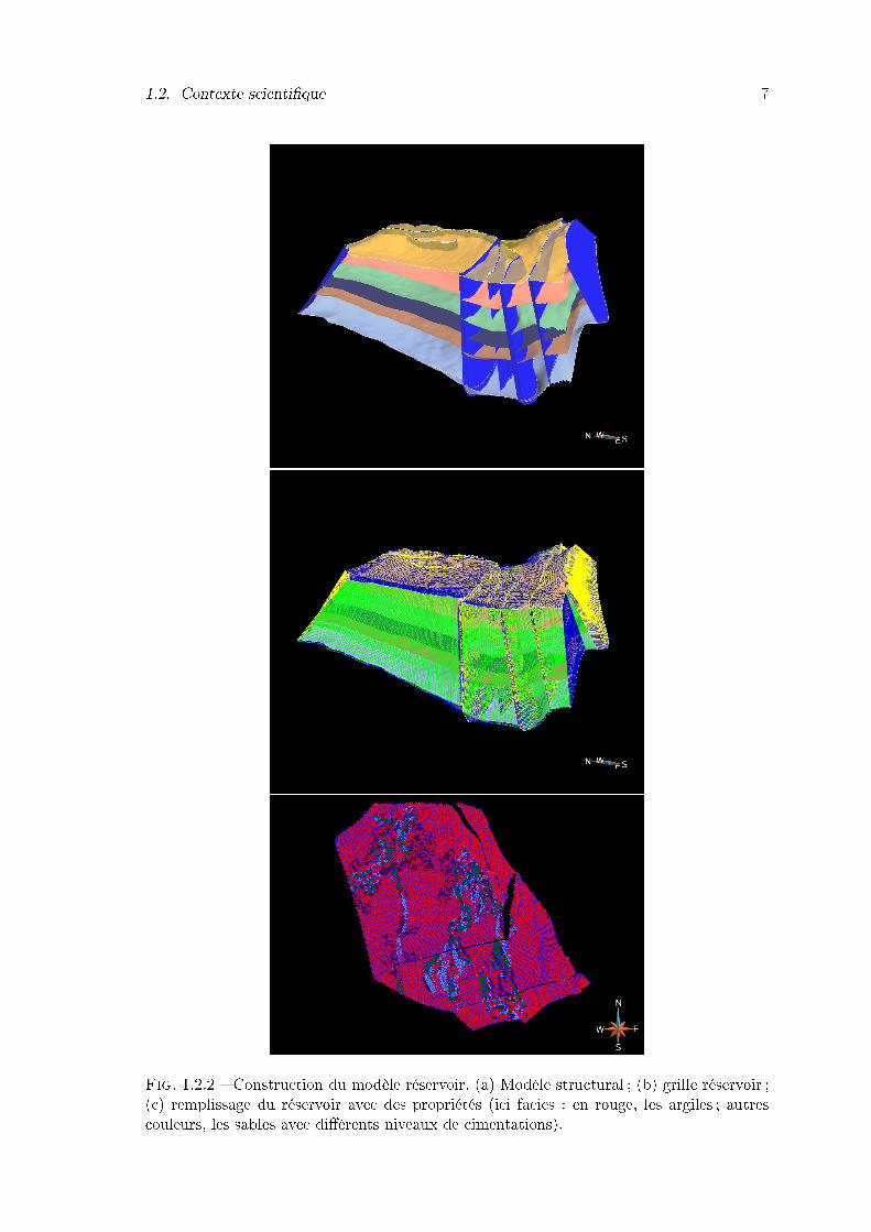
1.2.2 Construction du modèle réservoir. (a) Modèle structural ; (b) grille réser-voir ; (c) remplissage du réservoir avec des propriétés (ici facies : en rouge,les argiles ; autres couleurs, les sables avec di�érents niveaux de cimenta-tions). . . . . . . . . . . . . . . . . . . . . . . . . . . . . . . . . . . . . . . 7
2.2.1 La propagation d'une onde P sur une interface entre deux milieux induitla génération d'une onde P ré�échie Pr, d'une onde P transmise Pt, d'uneonde S ré�échie Sr et d'une onde S transmise St. . . . . . . . . . . . . . . 16
2.2.2 Les di�érentes approximations de l'équation de Zoeppritz. L'approxima-tion d'Aki et Richards, en pointillé vert, est retenue pour sa validité dansl'intervalle des angles considérés dans le domaine pétrolier. Tiré de Egre-teau 2005. . . . . . . . . . . . . . . . . . . . . . . . . . . . . . . . . . . . . 18
2.3.1 Localisation géographique du champ Alpha. . . . . . . . . . . . . . . . . . 212.3.2 Evolution stratigraphique des bassins o�shore angolais. De Brown�eld and
Charpentier 2006b. . . . . . . . . . . . . . . . . . . . . . . . . . . . . . . . 232.3.3 Interprétation géologique régionale du champ Alpha. . . . . . . . . . . . . 232.3.4 Vue 3D de la grille réservoir R-Alpha, avec une section sismique et l'em-
placement du puits. . . . . . . . . . . . . . . . . . . . . . . . . . . . . . . . 242.3.5 Deux couches de la grille réservoir R-Alpha. La propriété illustrée repré-
sente les faciès lithologiques : argiles en rouge, sables grossiers (en vert) à�ns (en bleu). La limite des données sismiques étudiées a été ajoutée surl'image. Le point blanc correspond à la position du puits W-Alpha. . . . . 25
2.3.6 Logs pétrophysiques, pétroélastiques et lithologiques deW-Alpha. De gaucheà droite : Gamma-Ray, lithologie, densité, vitesses P et S, porosité e�ectiveet saturation. . . . . . . . . . . . . . . . . . . . . . . . . . . . . . . . . . . 25
2.3.7 Diagramme croisé des propriétés Impédances relatives versus coe�cient dePoisson relatif, coloré par les facies au puits. . . . . . . . . . . . . . . . . . 26
2.3.8 Courbes d'enfouissement estimées pour le puits W-Alpha, pour les proprié-tés densité, vitesses P et S. Les points rouges correspondent aux donnéesdu puits W-Alpha, les points verts aux données du puits voisin. . . . . . . 27
2.3.9 Section sismique Near suivant la direction inline (à gauche) et crossline (àdroite). Le réservoir est individualisé par les horizons bleus et la trajectoiredu puits est représentée en jaune. . . . . . . . . . . . . . . . . . . . . . . . 28
2.3.10 Ondelettes obtenues par calibration au puits sur le stack complet des don-nées sismiques (à gauche), sur les stacks proches et moyens o�sets (à droite). 28
2.3.11 Sections en impedances P (à gauche) et S (à droite) pour les inversionsdeterministes (en haut) et stochastiques (en bas). L'inversion stochastiqueest réalisée uniquement sur le réservoir R-Alpha. . . . . . . . . . . . . . . 29
2.4.1 Localisation géographique du champ Beta. . . . . . . . . . . . . . . . . . . 30
xi

xii Table des �gures
2.4.2 Interprétation géologique régionale du champ Bêta, d'après Corredor et al.2005. . . . . . . . . . . . . . . . . . . . . . . . . . . . . . . . . . . . . . . . 31
2.4.3 Interprétation géologique du réservoir R-Bêta avec une section temps desdonnées sismiques (à gauche). . . . . . . . . . . . . . . . . . . . . . . . . . 32
2.4.4 Vue 3D (à gauche) et section transversale (à droite) de la grille réservoirR-Bêta, avec une section sismique et l'emplacement des puits. La propriétéreprésentée est le Net-To-Gross. . . . . . . . . . . . . . . . . . . . . . . . . 32
2.4.5 Deux couches de la grille réservoir R-Bêta. La propriété illustrée représentele Net-To-Gross. La limite des données sismiques étudiées a été ajoutée surl'image. Les points blancs correspondent aux positions des puits W-Bêta1à W-Bêta5. . . . . . . . . . . . . . . . . . . . . . . . . . . . . . . . . . . . 33
2.4.6 Implantation des puits du champ Bêta dans les intervalles chenalisés duréservoir. . . . . . . . . . . . . . . . . . . . . . . . . . . . . . . . . . . . . . 33
2.4.7 Logs lithologiques et pétroélastiques (lithologie, densité, vitesses P et S)pour les cinq puits du champ Bêta. . . . . . . . . . . . . . . . . . . . . . . 34
2.4.8 Diagramme croisé des propriétés Impédances acoustiques et du coe�cientde Poisson, coloré par les 12 faciès initiaux, pour le puits W-Bêta3 à gaucheet pour tous les puits à droite. . . . . . . . . . . . . . . . . . . . . . . . . . 35
2.4.9 Comparaison des logs réels (en noir) et simulés par le PEM (en rouge) pourVp, pour tous les puits du champ Bêta. . . . . . . . . . . . . . . . . . . . . 35
2.4.10 Section sismique Near suivant la direction inline (à gauche) et crossline (àdroite). Le réservoir est individualisé par les horizons rouge et orange et latrajectoire des puits est représentée en rouge. . . . . . . . . . . . . . . . . 36
2.4.11 Ondelettes obtenues par calibration aux puits sur les di�érents substacks.En mauve : ondelette near ; en rouge : ondelette mid1 ; en vert : ondelettemid2 ; en jaune : ondelette far. . . . . . . . . . . . . . . . . . . . . . . . . . 37
2.4.12 Sections en impedances P (à gauche) et S (à droite) pour les inversionsdeterministes (en haut) et stochastiques (en bas). L'inversion stochastiqueest réalisée uniquement sur le réservoir R-Bêta. . . . . . . . . . . . . . . . 37
2.5.1 Principes de la dolomitisation hydrothermale dans les niveaux non per-méables du réservoir Gamma. . . . . . . . . . . . . . . . . . . . . . . . . . 40
3.3.1 Cellules des maillages "CPG" (irrégulier structuré) et cartésiens (régulierstructuré). . . . . . . . . . . . . . . . . . . . . . . . . . . . . . . . . . . . . 47
3.3.2 Transformation d'une cellule réservoir en une série de voxels (cellules duvoxet). . . . . . . . . . . . . . . . . . . . . . . . . . . . . . . . . . . . . . . 47
3.3.3 L'intersection de la grille réservoir (exemple du champ Alpha) avec unpseudo puits (en rouge) permet de récupérer les propriétés du réservoirsans changement d'échelle. . . . . . . . . . . . . . . . . . . . . . . . . . . . 48
3.4.1 E�et du changement d'échelle entre les di�érents supports d'informationsur le champ Alpha. En haut, impédances P à l'échelle sismique ; au centre,les mêmes impédances P portées dans la grille réservoir ; en bas, les impé-dances portées de la grille vers le voxet. . . . . . . . . . . . . . . . . . . . 49
3.4.2 Statistiques du changement d'échelle entre les di�érents supports d'infor-mation sur le champ Alpha. En haut, nombre d'échantillons moyennés parcellule du réservoir ; la zone bleue correspond à des cellules de plus grandetaille ; en bas, écart-type des échantillons, en pourcentage. . . . . . . . . . 50
Table des �gures xiii
3.4.3 E�et du changement d'échelle sur une trace sismique. (a) l'impédance Pde l'inversion stochastique à l'échelle sismique, (b) l'impédance P dans levoxet, (c) trace sismique réelle, (d) synthétique obtenu à partir de a, (e)synthétique du voxet obtenu à partir de b et (f) di�érence entre les deuxsynthétiques. . . . . . . . . . . . . . . . . . . . . . . . . . . . . . . . . . . 51
3.4.4 E�et du changement d'échelle sur les sections sismiques. En haut, la sec-tion issue de la modélisation sur le volume à l'échelle sismique (quelquescellules vides dans le volume d'impédance sismique apparaissent commedes points sur l'image sismique) ; en bas, la section issue de la modéli-sation sur le volume à l'échelle réservoir. Toutes ces modélisations sontréalisées par convolution 1D sur chacune des traces du volume 3D. Lestraces synthétiques de la �gure 3.4.3 ont été replacées sur la �gure. . . . . 52
3.5.1 Application d'un �ltre moyen sur un point donné et ses p traces de partet d'autre, en x et y. . . . . . . . . . . . . . . . . . . . . . . . . . . . . . . 53
3.5.2 Application d'un �ltre moyen sur la section sismique issue des propriétésdu PEM du champ Alpha. En haut, la section brute ; en bas, la section�ltrée. . . . . . . . . . . . . . . . . . . . . . . . . . . . . . . . . . . . . . . 54
3.5.3 Application d'un �ltre moyen sur la section sismique issue des propriétésdu PEM du champ Bêta. En haut, la section brute ; en bas, la section �ltrée. 55
3.6.1 Comparaison des données sismiques synthétiques et réelles du champ Bêta,basée sur les cartes de Kohonen, avec 20 neurones. A gauche, la classi�ca-tion des données synthétiques issues des résultats d'inversion portés dansla grille réservoir ; à droite, la classi�cation des données réelles. . . . . . . 56
3.6.2 Comparaison des données sismiques synthétiques et réelles, basée sur lescartes de Kohonen, avec 20 neurones. A gauche, la classi�cation des don-nées synthétiques issues du PEM ; à droite, la classi�cation des donnéesréelles ; en bas, la concordance des classes : bleu foncé si la classe est lamême sur les deux volumes, bleu clair sinon. . . . . . . . . . . . . . . . . . 58
4.1.1 Work�ow to evaluate the structural uncertainty e�ect on reservoir charac-terization. Seismic and well data are used to create a base case model.Multiple structural realizations are simulated using interpretation uncer-tainties. The rest of the study consists in inverting, then classifying theattributes to recover facies in the di�erent reservoir grids. . . . . . . . . . 63
4.2.1 Operating principle for the P-Fields simulation, applied on a surface. Anuncertainty value zsim(u) is added up to the initial surface at each nodeu. This value is drawn in the local CDF. From Thore et al. 2002. . . . . . 64
4.2.2 In�uence of the correlation length on the simulated horizons. The dottedred lines represent the uncertainty interval, the black line the referencehorizon. The blue and green lines are the simulated horizons respectivelyfor a small and a long correlation length. The simulation is constrained bytwo wells. . . . . . . . . . . . . . . . . . . . . . . . . . . . . . . . . . . . . 65
4.2.3 Misplaced grid layers versus references horizons, overlaid on Alpha Fieldseismic data. Reference horizons are blue, corresponding grid layers aregrey. Di�erences on the far right-hand side should not be taken into accountsince the reservoir grid is bigger than the geological formation. . . . . . . . 66
xiv Table des �gures
4.2.4 Computed di�erence maps between reference horizons and correspondinggrid layers, with their respective histograms. Di�erences on the far right-hand side should not be taken into account since the reservoir grid is biggerthan the geological formation. . . . . . . . . . . . . . . . . . . . . . . . . . 67
4.2.5 Statistical analysis from the structural simulation. The top panel givesfor each realization the rock volume. The bottom left panel shows thetriangular PDF and the right panel shows the CDF. The red marker oneach panel corresponds to the base case model. . . . . . . . . . . . . . . . 68
4.2.6 The eight structural models on which the rest of the study will take place.Respectively, the initial model, percentiles 0%, 5%, 10% (�srt line), 50%,90%, 95% and 100% (second line) are represented. . . . . . . . . . . . . . . 69
4.3.1 Original well logs in dark blue and �ltered logs with a gaussian �lter ingreen, respectively for P and S velocities and density. . . . . . . . . . . . . 71
4.3.2 Inversion results at well location for P (left) and S (right) impedances.Dark blue curves are the original P and S impedances. . . . . . . . . . . . 72
4.3.3 Inversion results for the initial model. Top : Actual seismic data, center :synthetic seismic data and bottom : residuals. . . . . . . . . . . . . . . . . 73
4.3.4 Inversion results for the initial model : an independent realization of P im-pedances versus the mean. The actual seismic is represented in the back-ground, as well as the P impedance log. . . . . . . . . . . . . . . . . . . . 74
4.4.1 Distribution of samples from two lithotypes in a space of two physical pro-perties z1 and z2. The probability densities for each group are representednear to the axes, showing signi�cant overlap between both groups. The dis-crimination is improved with linear combinations of the original variables.From Bosch et al. 2002. . . . . . . . . . . . . . . . . . . . . . . . . . . . . 75
4.4.2 Raw crossplot of Ip versus PR coloured by the 7 facies interpreted on thelogs. . . . . . . . . . . . . . . . . . . . . . . . . . . . . . . . . . . . . . . . 76
4.4.3 Raw crossplot of Ip versus PR coloured by the 5 new facies. . . . . . . . . 774.4.4 Crossplot of Ip versus PR coloured by facies, after removing the compac-
tion e�ect from both properties. . . . . . . . . . . . . . . . . . . . . . . . . 774.4.5 Crossplot of Ip and PR detrended, with polygons delimiting the clusters
for each facies. The composition of each cluster is shown in the pie-charts(from left to right, Facies 1 to Facies 5). . . . . . . . . . . . . . . . . . . . 78
4.4.6 Comparison between initial facies interpretation of well log data (left),with the facies interpretation of detrended properties at the seismic scale(right). . . . . . . . . . . . . . . . . . . . . . . . . . . . . . . . . . . . . . . 79
4.4.7 Crossplots of detrended Ip versus detrended PR coloured by facies : left :original well logs, center : �ltered logs in the seismic bandwidth, right :minicube from seismic attributes. . . . . . . . . . . . . . . . . . . . . . . . 79
4.4.8 PDF operator in the crossplot of detrended Ip versus detrended PR co-loured by facies : left : original well logs, center : �ltered logs in the seismicbandwidth, right : minicube from seismic attributes. . . . . . . . . . . . . 80
4.4.9 Probability cubes computed from the PDF operators. The �rst imageshows a slice of the actual seismic block through the main channel ofreservoir R-Alpha, along a horizon from the initial structural model. Theother images show a slice of the probability cubes for each facies. FaciesF1 range is between 0 and 100% ; for the other facies codes, the range isbetween 0 and 25%. . . . . . . . . . . . . . . . . . . . . . . . . . . . . . . . 81
Table des �gures xv
4.5.1 Slices of the F1 Probability cube along the main channel of R-Alpha andthe F1 most probable value in the initial reservoir grid. . . . . . . . . . . . 82
4.5.2 Facies repartition in the initial reservoir model, on layer 21, with di�erentshale thresholds in percent. . . . . . . . . . . . . . . . . . . . . . . . . . . 83
4.5.3 Facies repartition in the initial reservoir model, on layer 21, with the shalethreshold of 87%, determined from the well data calibration. . . . . . . . . 84
4.5.4 Facies repartition in the 21st layer of the structural models. The �rst lineshows the geological interpretation, the picture on the left of the secondline shows the facies repartition in the initial reservoir grid. . . . . . . . . 85
4.5.5 Facies repartition in the 105th layer of the structural models. The �rst lineshows the geological interpretation, the picture on the left of the secondline shows the facies repartition in the initial reservoir grid. . . . . . . . . 86
5.1.1 Schéma de fonctionnement des déformations graduelles. . . . . . . . . . . . 925.2.1 Les di�érentes formulations des déformations graduelles. Les images du
haut montrent une chaîne de réalisation réservoir à partir de l'équation debase des déformations graduelles. Au milieu, la formulation des déforma-tions graduelles structurales (la covariance change, mais pas la distributionde la propriété). Les images du bas montrent la formulation locale (seuleune petite partie du réservoir est réévaluée). De Hu et al. 1999. . . . . . . 95
5.2.2 Principe du krigeage des réalisations non conditionnées dans le proces-sus des déformations graduelles. La ligne 1 représente la simulation non-conditionnée avec le point de données et l'estimation par krigeage du point ;la ligne 2 montre la simulation conditionnée. . . . . . . . . . . . . . . . . . 97
5.3.1 Itérations 1 et 3 d'un processus par déformations graduelles. A l'itération1, l'ellipse représente la chaîne de réalisations produite en combinant Y1 etY2 sur l'exemple d'une grille réservoir à deux cellules. Le nuage de pointscorrespond à la loi de distribution de la propriété. Y3 représente la com-binaison dont la fonction coût est la plus faible pour cette itération. Lacroix indique le minimum global de la fonction coût. A l'itération 2, Y3 etY4 donnent Y5. A l'itération 3, Y5 et Y6 donnent Y7. . . . . . . . . . . . . . 99
5.3.2 Comportement type de la fonction coût pendant une itération donnée, enfonction de c. En c = 0, nous avons la réalisation initiale, en c = 1 laréalisation secondaire. En c = 0.05, on note un minima local de la fonctioncoût et en c = 0.95, le minima global (en rouge) qui correspond à laréalisation optimale de l'itération. . . . . . . . . . . . . . . . . . . . . . . . 101
5.4.1 Section de la grille réservoir pour la validation de la méthode d'inversionpar déformations graduelles. La propriété illustrée est la vitesse P du mo-dèle initial. La trajectoire du puits est signalée en rouge. . . . . . . . . . . 102
5.4.3 Vitesse P du modèle initial sur trois couches di�érentes dans le modèleréservoir. . . . . . . . . . . . . . . . . . . . . . . . . . . . . . . . . . . . . . 102
5.4.2 Application du PEM à l'échelle log : pour chaque faciès (colonne 1) et pourchaque log, on extrait les lois d'enfouissement. Les logs calculés, à l'échelleréservoir, reproduisent les logs initiaux. . . . . . . . . . . . . . . . . . . . . 103
5.4.4 Histogrammes de la densité (à gauche) et de la vitesse P (à droite) dumodèle initial. . . . . . . . . . . . . . . . . . . . . . . . . . . . . . . . . . . 103
5.4.5 Densité (à gauche) et vitesse P (à droite) réelles sur la couche 51 du modèleréservoir. . . . . . . . . . . . . . . . . . . . . . . . . . . . . . . . . . . . . . 104

xvi Table des �gures
5.4.6 Histogrammes de la densité (à gauche) et vitesse P (à droite) du modèleréelle. . . . . . . . . . . . . . . . . . . . . . . . . . . . . . . . . . . . . . . 105
5.4.7 Processus de l'anamorphose. A gauche : Porosité brute (en haut, histo-gramme ; en bas, la fréquence cumulée). A droite : Porosité transforméepar anamorphose (en haut, histogramme gaussien ; en bas, la fréquencecumulée gaussienne). . . . . . . . . . . . . . . . . . . . . . . . . . . . . . . 106
5.4.8 Fonction coût pour une inversion par déformations graduelles. Ici, la fonc-tion coût est calculée sur 300 itérations. La diminution de l'erreur entreréalisations initiales et �nales est de 69%. . . . . . . . . . . . . . . . . . . 107
5.4.9 Vitesse P (première ligne) et densité (deuxième ligne) pour les réalisationsinitiales (première colonne), �nales (deuxième colonne) et réelles sur lacouche 51 du modèle réservoir. . . . . . . . . . . . . . . . . . . . . . . . . . 108
5.4.10 Impédances pour les réalisations initiales (première colonne), �nales (deuxièmecolonne) et réelles sur la couche 20 du modèle réservoir. . . . . . . . . . . 108
5.4.11 Impédances pour les réalisations initiales (première colonne), �nales (deuxièmecolonne) et réelles sur la couche 40 du modèle réservoir. . . . . . . . . . . 109
5.4.12 Impédances pour les réalisations initiales (première colonne), �nales (deuxièmecolonne) et réelles sur la couche 50 du modèle réservoir. . . . . . . . . . . 109
5.4.13 Impédances pour les réalisations initiales (première colonne), �nales (deuxièmecolonne) et réelles sur la couche 80 du modèle réservoir. . . . . . . . . . . 109
5.4.14 Section en vitesse P pour les réalisations initiales (première colonne), �-nales (deuxième colonne) et réelles. . . . . . . . . . . . . . . . . . . . . . . 110
5.4.15 Comparaison des histogrammes initiaux, �naux et réels pour la vitesse(première ligne) et la densité (deuxième ligne). . . . . . . . . . . . . . . . . 110
5.4.16 Sections sismiques avant et après le processus d'inversion par déformationsgraduelles, et la sismique "réelle". . . . . . . . . . . . . . . . . . . . . . . . 111
5.4.17 Résidus avant et après le processus d'inversion par déformations graduelles. 1115.4.18 Réalisations en impédances pour les réalisations initiales (première co-
lonne), �nales (deuxième colonne) et réelles sur la couche 20 du modèleréservoir. La réalisation �nale avec plusieurs variogrammes (en bas) estcomparée à la réalisation �nale à un variogramme (en haut). . . . . . . . . 112
5.4.19 Réalisations en impédances pour les réalisations initiales (première co-lonne), �nales (deuxième colonne) et réelles sur la couche 40 du modèleréservoir. La réalisation �nale avec plusieurs variogrammes (en bas) estcomparée à la réalisation �nale à un variogramme (en haut). . . . . . . . . 113
5.4.20 Réalisations en impédances pour les réalisations initiales (première co-lonne), �nales (deuxième colonne) et réelles sur la couche 50 du modèleréservoir. La réalisation �nale avec plusieurs variogrammes (en bas) estcomparée à la réalisation �nale à un variogramme (en haut). . . . . . . . . 113
5.4.21 Réalisations en impédances pour les réalisations initiales, �nales et réellessur la couche 80 du modèle réservoir. La réalisation �nale avec plusieurs va-riogrammes (en bas) est comparée à la réalisation �nale à un variogramme(en haut). Les carrés rouges montrent une structure �ne correctement re-crée avec l'utilisation de plusieurs variogrammes. . . . . . . . . . . . . . . 114
5.4.22 Comparaison de la sismique réelle, la sismique synthétique "solution" etla sismique synthétique �nale du processus d'inversion par déformationgraduelle. . . . . . . . . . . . . . . . . . . . . . . . . . . . . . . . . . . . . 115
6.2.1 Work�ow for the supervised classi�cation with neural networks. . . . . . . 119

Table des �gures xvii
6.3.1 Example of learning phase for an Arti�cial Neural Network. An input vec-tor is given to the network. The winning neuron (in red) is determined,and then updated so as to be closer to the input data. . . . . . . . . . . . 121
6.3.2 Time varying input patterns such as seismic traces can not be evaluatedby Euclidian distance. Here the repetition of the same trace with time shiftwill be identi�ed as di�erent signals if the Euclidian distance is used. If weuse the correlation between the trace and the neuron, this series will beseen as the same sequence. . . . . . . . . . . . . . . . . . . . . . . . . . . . 122
6.4.1 A seismic section for the Beta �eld, showing the reservoir of interest deli-mited by the green horizons. . . . . . . . . . . . . . . . . . . . . . . . . . . 124
6.4.2 Geological correlation for the wells from Beta �eld. We can see the di�erentgeological bodies and how some markers appear or disappear laterally. . . 125
6.4.3 Correlation sheet for the wells from Beta �eld, with only some of the mar-kers shown, for clarity. The property shown here is Vp. . . . . . . . . . . . 125
6.4.4 Well log blocking results for well W-Beta3. This �gure shows the originallogs in black and the blocked logs in green for (a) the density ρ, (b) the Pvelocity Vp and (c) the S velocity Vs. The near seismic trace is comparedto (d) the synthetic of the blocked logs, (e) the synthetic of the originallogs. The well-to-seismic tie with the original logs is of poor quality. . . . . 126
6.4.5 Well log blocking optimization procedure for well W-Beta3. This �gureshows the original logs in black, the blocked logs in green and the optimizedlogs in red for (a) the density ρ, (b) the P velocity Vp and (c) the S velocityVs. The near seismic trace is compared to (d) the synthetic of the blockedlogs, (e) the synthetic of the best logs and (f) the synthetic of the originallogs. The well-to-seismic tie has been greatly improved. . . . . . . . . . . . 127
6.4.6 The normalized �tness function of the blocking optimization. . . . . . . . 1276.4.7 At each location U, for each parameter and each layer, the SGS method
draws values Y from the CCDF provided by the parameter statistics ex-tracted from the wells. . . . . . . . . . . . . . . . . . . . . . . . . . . . . . 128
6.4.8 The Massive Modeling. The sections are respectively ρ, Vp, Vs and thesynthetic seismograms. The horizontal scale is the trace number. . . . . . 129
6.4.9 Non supervised Kohonen maps realized with an interval thickness of 50msand 180ms, with 20 neurons. . . . . . . . . . . . . . . . . . . . . . . . . . . 130
6.4.10 Non supervised Kohonen maps with respectively 5, 20 and 50 neurons.Next to each map, we show the resulting neurons (for the 50 neurons map,we show only the second half). Some traces from the 50 neurons maprepresent noise. . . . . . . . . . . . . . . . . . . . . . . . . . . . . . . . . . 131
6.4.11 Non supervised Kohonen maps realized with neighbourhood radius of 1and 10 neurons. The �rst line shows the neuron repartition, the secondline the neurons. . . . . . . . . . . . . . . . . . . . . . . . . . . . . . . . . 132
6.4.12 Fitness map for the non supervised Kohonen maps realized with neighbou-rhood radius of 1 and 10 neurons. . . . . . . . . . . . . . . . . . . . . . . . 133
6.5.1 A small part of the Massive Modeling volume, with the neuron repartition(top line) and the �tness (bottom line) for each trace. . . . . . . . . . . . . 134
6.5.2 A small part of the color-coded visualization of the classi�cation. On thetop-row, the traces are shown as they are in the dataset. On the bottom-row, the traces are ordered by class and �tness. Since we show about 300traces, once ordered we see only a small portion of two classes on thebottom row. . . . . . . . . . . . . . . . . . . . . . . . . . . . . . . . . . . . 134

xviii Table des �gures
6.5.3 A graph showing the percentage of model traces exceeding the �tness onthe abscissa. For example, 50% of the model traces have a �tness greaterthan 90%, which is fully satisfactory. . . . . . . . . . . . . . . . . . . . . . 135
6.5.4 A part of the table for the classi�cation analysis. We obtain the parame-ter average and standard deviation for each neuron. Here are shown thethickness, ρ and Vp for the two �rst layers and the three �rst neurons. . . 135
6.5.5 Likelihood of each model traces with the synthetics of the �ve wells forBeta �eld. A likelihood of 1 is the best correlation value between a modeltrace and a synthetic trace. . . . . . . . . . . . . . . . . . . . . . . . . . . 136
6.5.6 Predictive modeling : the model traces from the training phase have beenapplied to the actual seismic traces. The maps show the classi�cation andthe �tness. The white circle on the �tness map gives the location of wellW-Beta1. . . . . . . . . . . . . . . . . . . . . . . . . . . . . . . . . . . . . 137
6.5.7 Likelihood of each model traces with the actual seismic trace of the �vewells for Beta �eld. . . . . . . . . . . . . . . . . . . . . . . . . . . . . . . . 138
6.5.8 Descrictive modeling : the training phase has been performed on the actualseismic traces. The maps show the classi�cation and the �tness. . . . . . . 139
6.5.9 Likelihood of each model traces with the actual seismic trace at the �vewells for Beta �eld. . . . . . . . . . . . . . . . . . . . . . . . . . . . . . . . 140
6.5.10 Graph showing the percentage of model traces exceeding the �tness on theabscissa. For example, 60% of the model traces have a �tness greater than50%. . . . . . . . . . . . . . . . . . . . . . . . . . . . . . . . . . . . . . . . 140
6.5.11 A small part of the color-coded visualization of the classi�cation. The colorsdisplayed on the top row are quite dull, this means that the �tness for thetraces presented here is low. See �gure 6.5.2 . . . . . . . . . . . . . . . . . 141
6.5.12 Likelihood of each model traces with the synthetic traces of the �ve wellsfor Beta �eld. . . . . . . . . . . . . . . . . . . . . . . . . . . . . . . . . . . 141
6.5.13 The classi�cation map from the petrophysical training with geological in-terpretation on top, with structural interpretation on the bottom picture. 142
6.5.14 The classi�cation map from the seismic training with geological interpre-tation on the top, with structural interpretation on the bottom. . . . . . . 143
6.6.1 Well log blocking results. This �gure shows the original logs in black andthe blocked logs in green for (a) the density ρ, (b) the P velocity Vp and (c)the S velocity Vs. The near seismic trace is compared to (d) the synthetic ofthe blocked logs, (e) the synthetic of the original logs. The well-to-seismictie with the original logs is of poor quality. . . . . . . . . . . . . . . . . . . 146
6.6.2 Well log blocking optimization procedure. This �gure shows the originallogs in black, the blocked logs in green and the optimized logs in red for(a) the density ρ, (b) the P velocity Vp and (c) the S velocity Vs. The nearseismic trace is compared to (d) the synthetic of the blocked logs, (e) thesynthetic of the best logs and (f) the synthetic of the original logs. Thewell-to-seismic tie has been greatly improved. . . . . . . . . . . . . . . . . 146
6.6.3 The Massive Modeling. The sections are respectively ρ, Vp, Vs and thesynthetic seismograms. . . . . . . . . . . . . . . . . . . . . . . . . . . . . . 147
6.6.4 Non supervised Kohonen maps realized with an interval thickness of 50msand 100ms. . . . . . . . . . . . . . . . . . . . . . . . . . . . . . . . . . . . 148
Table des �gures xix
6.6.5 Non supervised Kohonen maps with respectively 5, 30 and 50 neurons.Next to each map, we show the resulting neurons (for the 50 neurons map,we show only the second half). Some traces from the 50 neurons maprepresent noise. . . . . . . . . . . . . . . . . . . . . . . . . . . . . . . . . . 149
6.6.6 Non supervised Kohonen maps realized with neighbourhood radius of 1and 10 neurons. The �rst line shows the neuron repartition, the secondline the neurons. The last line shows the �tness. . . . . . . . . . . . . . . . 150
6.7.1 A small part of the Massive Modeling volume, with the neuron repartition(top line) and the �tness (bottom line) for each trace. . . . . . . . . . . . . 151
6.7.2 A small part of the color-coded visualization of the classi�cation. The colorsdisplayed on the top row are very bright, this means that the �tness forthe traces presented here is high. See �gure 6.5.2 for explanation. . . . . . 152
6.7.3 Graph showing the percentage of model traces exceeding the �tness on theabscissa. 70% of the model traces have a �tness equal or greater than 80%,which is fully satisfactory. . . . . . . . . . . . . . . . . . . . . . . . . . . . 152
6.7.4 Part of the classi�cation analysis table, showing the parameter average andstandard deviation for each neuron. Here are shown the thickness, ρ andVp for the two �rst layers and the four �rst neurons. . . . . . . . . . . . . 153
6.7.5 Likelihood of each model traces with the synthetic traces of the twelvewells for Gamma �eld. . . . . . . . . . . . . . . . . . . . . . . . . . . . . . 153
6.7.6 Predictive modeling : the model traces from the training phase have beenapplied to the actual seismic traces. The maps show the classi�cation andthe �tness. The location of the two well clusters has been removed forcon�dentiality. . . . . . . . . . . . . . . . . . . . . . . . . . . . . . . . . . . 154
6.7.7 Likelihood of each model traces with the actual seismic trace at the welllocation for Gamma Field. . . . . . . . . . . . . . . . . . . . . . . . . . . . 155
6.7.8 Descriptive modeling : the training phase has been performed on the actualseismic traces. The maps show the classi�cation and the �tness. . . . . . . 156
6.7.9 Likelihood of each model traces with the synthetic traces of the well loca-tion for Gamma Field. . . . . . . . . . . . . . . . . . . . . . . . . . . . . . 157
6.7.10 Graph showing the percentage of model traces exceeding the �tness on theabscissa. For example, 70% of the model traces have a �tness greater than70%. . . . . . . . . . . . . . . . . . . . . . . . . . . . . . . . . . . . . . . . 158
6.7.11 A small part of the color-coded visualization of the classi�cation. The colorsof some groups of traces displayed on the top row are quite dull, this meansthat the �tness for these traces is low. See �gure 6.5.2 for explanation. . . 158
6.7.12 Likelihood of each model traces with the synthetic traces of the twelvewells for Gamma �eld. . . . . . . . . . . . . . . . . . . . . . . . . . . . . . 159
6.7.13 The classi�cation map from the petrophysical training with geological in-terpretation on top, with structural interpretation on the bottom picture. 160
6.7.14 The classi�cation map from the seismic training with geological interpre-tation on the top, with structural interpretation on the bottom. . . . . . . 161
Liste des tableaux
4.1 Reference horizons and corresponding grid layers, with their uncertaintiesand correlation factors. . . . . . . . . . . . . . . . . . . . . . . . . . . . . . . 66
4.2 Simulated structural models chosen by percentile from �gure 4.2.5. Percen-tile 81% corresponds to the base case model. . . . . . . . . . . . . . . . . . . 69
5.1 Etapes permettant la construction d'une réalisation gaussienne par la mé-thode de simulation FFT-MA. . . . . . . . . . . . . . . . . . . . . . . . . . . 96
5.2 Relations V p − ρ de Gardner par lithologies pour l'équation ρ = dV fp . Les
unités sont km/s et g/cm3 . . . . . . . . . . . . . . . . . . . . . . . . . . . . 1045.3 Paramètres des trois processus successifs d'inversion par déformation gra-
duelle, pour évaluer l'impact du variogramme sur les résultats �naux. . . . . 112

Chapitre 1
Introduction générale
1.1 ProblématiqueLes modèles de réservoirs pétroliers jouent un rôle de plus en plus prépondérant dans
l'industrie pétrolière. Ils sont utilisés tout le long de la vie d'un gisement pour plani�er lesétudes complémentaires à e�ectuer, pour optimiser l'implantation de nouveaux puits, maisaussi et surtout, estimer les réserves d'hydrocarbures en place et simuler l'exploitation duprospect réel.Pour faire tout cela, les spécialistes ont besoin de connaître les propriétés-clés qui per-mettront d'expliquer (et donc de reproduire) les phénomènes physiques qui gouvernentle réservoir. Ils ont à leur disposition un certain nombre de données qui leur permettentd'obtenir ces propriétés, soit de manière directe, soit de manière indirecte. Les travaux decaractérisation réservoir s'appuient essentiellement sur deux types de données : les diagra-phies et les données sismiques.
Les diagraphies : Une diagraphie ("well log") consiste à mesurer, pendant (diagraphiesinstantanées) ou après (diagraphies di�érées) un forage, les caractéristiques des rochestraversées, à l'aide de di�érentes sondes. La diagraphie représente en général toutenregistrement d'une caractéristique d'une formation géologique en fonction de laprofondeur. Les diagraphies instantanées, enregistrées pendant le forage ("LWD :Logging While Drilling"), permettent de récupérer, lorsqu'elles traversent un milieu :� la teneur en hydrocarbures et/ou eau ;� la porosité ;� la perméabilité.Les diagraphies di�érées peuvent enregistrer les caractéristiques complémentaires,par exemples d'un milieu :� la vitesse de propagation d'une onde P ;� la densité de la formation ;� la résistivité ;� la radioactivité naturelle.Les mesures diagraphiques permettent l'estimation du contenu des réservoirs traver-sés, du pendage des couches, mais aussi de comparer les puits entre eux. Elles sontdéterminantes dans l'évaluation de la qualité économique du réservoir.Toutes ces propriétés sont essentielles pour simuler la vie du réservoir et les spé-
1

2 Chapitre 1. Introduction générale
cialistes cherchent donc à les intégrer dans les modèles. Cependant, les diagraphiesfournissent des informations très locales, car limitées à l'emplacement des puits, etces derniers ne sont présents qu'en petit nombre sur toute la surface d'un prospect.Les modèles de réservoirs calibrés à partir de ces données diagraphiques sont doncmal conditionnés dès que l'on s'éloigne des puits.Il est donc évident que les diagraphies ne su�sent pas pour contraindre les modèlesde réservoir.
Les données sismiques : La sismique est une technique de mesure indirecte qui consisteà enregistrer en surface des échos issus de la propagation dans le sous-sol d'une ondesismique provoquée. Ces échos sont générés par les hétérogénéités du sous-sol et semanifesteront par la présence de ré�ecteurs sur les enregistrements. Le temps d'arri-vée de l'écho permet de situer dans l'espace la position d'un ré�ecteur et l'amplitudeapporte des informations indirectes sur certains paramètres physiques.Après un traitement adapté, les données sismiques nous donnent une image de lastructure du sous-sol, ainsi que des informations sur sa nature.Les données sismiques représentent des mesures avec une bonne couverture spatialesur l'ensemble du prospect. Leur utilisation est couramment mise en avant lors dela construction de l'enveloppe géométrique d'un modèle réservoir. En revanche, lesinformations qu'elles contiennent en terme de paramètres physiques importants pourla description du réservoir sont largement sous-utilisées.
L'intégration quantitative des données sismiques dans les modèles de réservoir, comme nou-velle contrainte des propriétés loin des puits, est une approche de plus en plus étudiée denos jours. Le travail de cette thèse s'inscrit dans cette optique, et a pour but d'améliorerla cohérence entre les modèles de réservoirs et les données sismiques.La caractérisation réservoir est un domaine multidisciplinaire qui consiste à décrire la na-ture des roches qui contiennent des hydrocarbures. Elle se base sur l'expertise de l'ingénierieréservoir, de la géologie et de la géophysique dont les données doivent être intégrée dans ladescription du réservoir. Les méthodes qui permettent de réaliser cette intégration relèventessentiellement de la géostatistique. On pourra trouver une description de ces méthodesdans Doyen 2007 et Dubrule 2003. Les principaux enjeux de la caractérisation réservoirsont : comprendre le réservoir, le caractériser en retrouvant les propriétés qui vont in�uerson comportement, et prévoir son évolution dynamique au cours de la production.Le processus traditionnel de caractérisation réservoir consiste à intégrer autant d'informa-tions que possible dans un modèle géologique, qui correspond à un objet tridimensionnel�nement maillé. L'intégration des di�érents types de données, tels que les données sis-miques, les données de puits, les carottes et les données de production, est un sujet derecherche actif pour caractériser les réservoirs. L'importance de chaque information ne re-pose pas sur son utilisation seule, mais sur sa valeur ajoutée dans l'analyse d'un ensemblede données.Les approches utilisées actuellement impliquent l'intégration des données sismiques, puis-qu'elles constituent le seul volume de données couvrant l'intégralité du réservoir. Les don-nées de puits, carottes et données de production sont des données ponctuelles qui nousdonnent une vue directe sur les propriétés du réservoir à l'emplacement des puits. Lespropriétés fournies par ces trois types de données servent alors à mettre en cohérence lesdonnées sismiques et le réservoir.

1.2. Contexte scienti�que 3
La validation du réservoir passe par une phase de simulation de l'écoulement des �uidespour créer une courbe de production qui doit être comparable à la courbe réelle si le réser-voir est correctement déterminé. On e�ectue pour cela un changement d'échelle du modèlegéologique au modèle réservoir de maillage plus grossier. Si l'on parvient à reconstituer sacourbe de production, cela signi�e que le modèle est l'une des solutions envisageables pourle réservoir réel. En revanche, si les courbes de production réelles et simulées di�èrent, ilfaut revenir au modèle et le modi�er. Cette validation dynamique est di�cile à mettre enoeuvre car la courbe de production n'indique pas où les erreurs se trouvent dans le modèleréservoir. De plus, elle est coûteuse puisqu'il s'agit d'entrer le modèle de réservoir, très vo-lumineux et très complexe, dans un simulateur d'écoulement qui reproduit le mouvementdes �uides (comportement dynamique) à travers le réservoir pendant son exploitation, ainsique la production du champ étudié.Dans le cadre de cette thèse, nous proposons une approche complémentaire qui consisteà travailler directement sur le modèle réservoir dynamique. Nous présentons donc dansce manuscrit des méthodes de caractérisation réservoir qui visent à intégrer l'informationdans le modèle réservoir, sans passer par le modèle géologique, ce qui évite le changementd'échelle entre ces deux supports.Pour valider le réservoir, nous choisissons d'évaluer la qualité du modèle réservoir parla reconstitution des données sismiques. Il s'agit donc d'une validation statique, car cettevalidation est faite avec un volume unique de données sismiques. Cette approche a l'avan-tage de rendre le modèle réservoir cohérent avec la sismique.Cela signi�e qu'à partir de la géométrie et des propriétés du réservoir, un volume sismiquesynthétique est créé et comparé aux données sismiques réelles. Les propriétés statiques dumodèle réservoir peuvent donc être validées de cette manière, ce qui réduit leur niveaud'incertitudes pour la phase de simulation dynamique. En revanche, la comparaison entresismique réelle et synthétique n'est pas triviale.En e�et, la création d'un volume sismique synthétique suppose de connaître la fonctionde transfert entre les propriétés du réservoir et la sismique (de la physique des roches auxdonnées sismiques) et cela est loin d'être le cas. En revanche, nous pouvons faire appel àdes méthodes existantes pour transformer les propriétés du réservoir en propriétés signi�-catives pour la sismique (propriétés élastiques) et ensuite créer une sismique synthétiqueidéalisée. Cela implique donc que les données sismiques synthétiques et réelles ne sont pasdirectement comparables.Un autre problème concerne la di�érence des échelles d'observation pour les di�érentssupports d'information. En e�et, entre les données de puits, les données sismiques et lesmodèles de réservoir, les informations ne sont pas stockées au même niveau de détail. Il estdonc important de se pencher sur ce problème pour assurer la compatibilité des di�érentesdonnées entre elles, sachant que le support d'information �nal est le modèle réservoir. Lesméthodes que nous proposons abordent d'une manière ou d'une autre cette thématique dechangement d'échelle.
1.2 Contexte scienti�queCette partie synthétise les concepts de base pour la caractérisation réservoir. Une des-
cription des étapes de la construction du modèle réservoir y est présentée, de même queles principaux enjeux et écueils de l'ingénierie réservoir. Les di�érents modèles physiques

4 Chapitre 1. Introduction générale
qui nous permettent de simuler les propriétés réservoirs sont brièvement décrits.
1.2.1 L'ingénierie du réservoir pétrolierUn réservoir pétrolier est une formation rocheuse perméable dont l'espace poreux est
partiellement saturé par des hydrocarbures (huile, gaz). Au terme d'une migration depuisla zone de formation des hydrocarbures, appelée roche mère, ceux-ci viennent se piégerdans le réservoir en raison de l'imperméabilité des couches supérieures limitant ce dernierou du piège formé par la disposition des couches stratigraphiques. Le �uide saturant lespores interconnectés possède une liberté de mouvement par rapport au solide environnant.La physique associée aux milieux poreux est décrite par Mavko et al. 2003, qui parlent desrelations théoriques et empiriques entre la physique des roches, et les données sismiques.Pendant toute la durée de l'étude d'un champ pétrolier, les caractéristiques du réservoirsont continuellement estimées et synthétisées dans un modèle qui nous permet de repro-duire le comportement du réservoir réel et d'anticiper son comportement futur. Ainsi, lesspécialistes sont capables de déterminer à quel moment de la vie du champ il faut, parexemple, installer un puits d'injection pour réactiver la déplétion du réservoir, ou encorecombien de temps le champ pourra encore être exploité.Le modèle de réservoir représente donc la somme des connaissances disponibles, à savoir lesdonnées sismiques, de puits, leurs interprétations, etc . . . Plus cette connaissance s'enrichitet plus les incertitudes liées au réservoir diminuent. Nous résumons ci-après l'état de l'artsur le réservoir pétrolier.
1.2.1.1 Le développement du réservoirLa délinéation d'un réservoir pétrolier est la première phase de développement de celui-
ci, puisqu'il s'agit de l'identi�cation du réservoir. Les données sont rassemblées pour dé�nirun premier modèle de réservoir. Ainsi, les prélèvements sur les carottes vont permettred'établir les caractéristiques pétrophysiques locales ; les diagraphies nous permettent d'ob-tenir des pro�ls de faciès géologiques, les premières relations entre les propriétés pétrophy-siques et les propriétés de physique des roches ; les données sismiques donneront lieu auxinterprétations structurales du réservoir dans un premier temps, puis à des interprétationsen terme de contenu de �uides par la suite.La création du premier modèle réservoir permet de faire les premières études de sensi-bilité de la sismique aux paramètres pétrophysiques et donne une estimation des réservesd'hydrocarbures. Si le gisement est économique, il sera mis en production. Cela consistetout d'abord à installer un certain nombre de puits (dits puits de production) à des endroitsstratégiques (dôme du réservoir par exemple). La pression interne du réservoir engendreune déplétion naturelle du réservoir, de courte durée. D'autres puits (puits d'injection)peuvent ensuite être installés pour assister la récupération des hydrocarbures.L'injection de �uides, deuxième étape du développement, permet de maintenir la pressioninterne du réservoir. Ceci active la phase d'étude dynamique du réservoir. Les propriétésliées à l'écoulement des �uides, la géologie et la connectivité entre les puits vont permettred'améliorer le modèle de réservoir.

1.2. Contexte scienti�que 5
1.2.1.2 La caractérisation réservoirLa caractérisation réservoir est la discipline centrée sur la compréhension des méca-
nismes physiques du réservoir. Elle s'applique dès les premières étapes du développementdu champ, et se poursuit jusqu'à l'arrêt de la production.La caractérisation réservoir est basée sur le modèle développé lors de la délinéation dugisement, comme mentionné plus haut, et correspond à la synthèse de toutes les donnéesdisponibles.Le modèle de réservoir se divise en deux parties :
� Le modèle statique qui décrit les propriétés du réservoir à l'équilibre (à un instantdonné). Le modèle statique synthétise les informations provenant des di�érents typesde données (puits, sismiques, carottes). L'ingénieur réservoir qui s'occupe de cettesynthèse doit donc mettre en cohérence toutes ces données qui ne se trouve pas surle même support d'information.
� Le modèle dynamique qui vise à reproduire le déplacement des �uides à travers leréservoir et la courbe de production (calage d'historique de production).
Pour le reste de la thèse, nous nous focaliserons sur le modèle statique, et toutes référencesultérieures aux modèles de réservoirs concerneront la partie statique.La construction du modèle d'un réservoir se fait généralement en trois étapes (voir �gure1.2.2) :
� La construction du modèle structural :La trame géométrique du réservoir est obtenue par l'interprétation des données sis-miques, en terme d'histoire dépositionnelle et tectonique, croisée avec l'interprétationdes puits, sur le positionnement des unités stratigraphiques. Le modèle structuralnous donne l'enveloppe, l'extension du réservoir, les objets géologiques présents, ainsique les extensions des failles et les contacts entre les �uides (eau, huile, gaz).Pour l'obtenir, on procède au pointé des horizons et des failles sur un volume sis-mique. On obtient alors des nuages de points dé�nissant une surface tridimension-nelle dans l'espace. Ces données surfaciques nous donne une première visualisationdu réservoir (image du haut sur la �gure 1.2.2).
� La construction de la grille réservoir :Le modèle de réservoir peut être discrétisé en une grille composée de blocs élémen-taires. La grille réservoir est un maillage tridimensionnel complexe, dé�ni générale-ment en profondeur et dont chaque cellule est renseignée par les propriétés qui nousintéressent, à savoir les propriétés pétrophysiques et pétroélastiques. Les couches dela grille réservoir suivent les couches géologiques. Le maillage généralement utilisépour décrire les grilles réservoirs est un maillage structuré irrégulier car il permet dereproduire assez �dèlement les objets géologiques (image centrale sur la �gure 1.2.2).Il s'agit d'un maillage composé de cellules hexaédriques dont les huit sommets sontancrés sur les piliers (piliers et horizons forment le squelette de la grille réservoiravant maillage).Typiquement, on trouvera une grille de plusieurs centaines de milliers (voire plu-sieurs millions) de cellules, dont la dimension latérale est de 50 à 100 mètres, etl'épaisseur de 1 à 15 mètres (soit 1 à 5 ms pour les grilles dé�nies en temps).

6 Chapitre 1. Introduction générale
� Le remplissage du modèle réservoir :Il existe deux approches principales pour remplir le réservoir de propriétés pétro-physiques. La première consiste à dé�nir un modèle de faciès dans la grille réservoir(image du bas sur la �gure 1.2.2). Ce modèle exprime l'historique dépositionnel enterme de lithologie. Par exemple, un chenal se matérialisera sous la forme de facièssableux plus ou moins cimentés, saturés en eau ou en huile. À partir des relationsétablies entre faciès et pétrophysique au niveau des puits, les propriétés réservoirs(perméabilité, porosité, saturation, etc...) sont attribuées à chaque faciès en fonctionde sa position dans le réservoir (relations basées sur la profondeur, l'unité géolo-gique,...).La deuxième approche consiste à intégrer dans le réservoir l'information issue d'uneinversion sismique en étudiant les relations entre les propriétés d'intérêt et les attri-buts de l'inversion.
Quelle que soit l'approche utilisée, le modèle réservoir doit être continuellement remis encause, pour chaque nouvelle donnée acquise à intégrer au modèle. Cette mise à jour estdi�cile à mettre en place, conséquence de la complexité des phénomènes physiques quis'appliquent aux réservoirs.
1.2.1.3 Les écueils sur le modèle réservoirLe modèle réservoir est construit à partir de toutes les données disponibles. Ces données
doivent être utilisées avec soin, car chaque donnée apporte son lot d'incertitudes. Nousfaisons ici référence au changement d'échelle entre les di�érents supports, et à la conversiontemps/profondeur.
La conversion temps/profondeur Le modèle de réservoir a généralement pour �na-lité la simulation des écoulements des �uides à travers le réservoir et la simulation desdonnées de production. Il est donc fréquemment dé�ni en profondeur, alors que les don-nées sismiques, utilisées dans les premières étapes de la construction du modèle réservoir,sont acquises, traitées et interprétées en temps, parfois migrées en profondeur. Le modèlesurfacique dé�ni sur ces données est construit en temps, puis transféré dans le domaineprofondeur. Il est alors nécessaire de véri�er que les horizons interprétés sur la sismiquecorrespondent à leurs emplacements mesurés aux puits. Dans le cas contraire, le modèlede conversion temps-profondeur doit être ajusté. L'utilisation d'un cube sismique migré enprofondeur ne permet pas d'éluder complètement ce problème, car le résultat de la migra-tion dépend du modèle de vitesse utilisé.Le maillage du modèle est ensuite assuré par des géomodeleurs, et cette opération pro-voque des transformations non bijectives entre le modèle surfacique et la grille réservoir(par exemple, décalage des horizons en regard du maillage, déplacement des plans de faille).Ces transformations peuvent provoquer des problèmes d'ajustements par la suite entre lemodèle réservoir et les données sismiques (HadjKacem 2006).La qualité des calages entre les données de puits, les données sismiques et le modèle ré-servoir sera déterminante pour l'utilisation, par la suite, des données sismiques pour leremplissage de la grille réservoir.
Le rééchantillonnage des données de puits Les puits nous donnent accès à l'infor-mation directe mais ponctuelle des propriétés réservoir à un endroit donné. Comme nous
1.2. Contexte scienti�que 7
Fig. 1.2.2 � Construction du modèle réservoir. (a) Modèle structural ; (b) grille réservoir ;(c) remplissage du réservoir avec des propriétés (ici facies : en rouge, les argiles ; autrescouleurs, les sables avec di�érents niveaux de cimentations).
8 Chapitre 1. Introduction générale
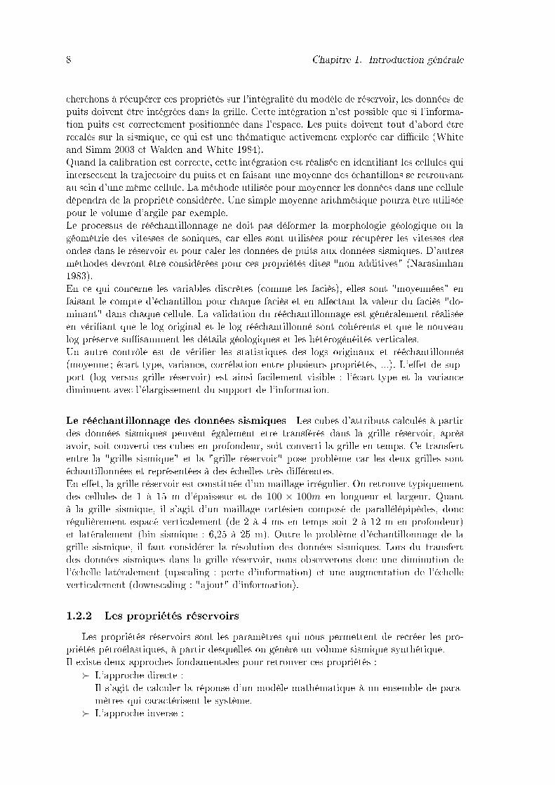
cherchons à récupérer ces propriétés sur l'intégralité du modèle de réservoir, les données depuits doivent être intégrées dans la grille. Cette intégration n'est possible que si l'informa-tion puits est correctement positionnée dans l'espace. Les puits doivent tout d'abord êtrerecalés sur la sismique, ce qui est une thématique activement explorée car di�cile (Whiteand Simm 2003 et Walden and White 1984).Quand la calibration est correcte, cette intégration est réalisée en identi�ant les cellules quiintersectent la trajectoire du puits et en faisant une moyenne des échantillons se retrouvantau sein d'une même cellule. La méthode utilisée pour moyenner les données dans une celluledépendra de la propriété considérée. Une simple moyenne arithmétique pourra être utiliséepour le volume d'argile par exemple.Le processus de rééchantillonnage ne doit pas déformer la morphologie géologique ou lagéométrie des vitesses de soniques, car elles sont utilisées pour récupérer les vitesses desondes dans le réservoir et pour caler les données de puits aux données sismiques. D'autresméthodes devront être considérées pour ces propriétés dites "non additives" (Narasimhan1983).En ce qui concerne les variables discrètes (comme les faciès), elles sont "moyennées" enfaisant le compte d'échantillon pour chaque faciès et en a�ectant la valeur du faciès "do-minant" dans chaque cellule. La validation du rééchantillonnage est généralement réaliséeen véri�ant que le log original et le log rééchantillonné sont cohérents et que le nouveaulog préserve su�samment les détails géologiques et les hétérogénéités verticales.Un autre contrôle est de véri�er les statistiques des logs originaux et rééchantillonnés(moyenne ; écart-type, variance, corrélation entre plusieurs propriétés, ...). L'e�et de sup-port (log versus grille réservoir) est ainsi facilement visible : l'écart-type et la variancediminuent avec l'élargissement du support de l'information.
Le rééchantillonnage des données sismiques Les cubes d'attributs calculés à partirdes données sismiques peuvent également être transférés dans la grille réservoir, aprèsavoir, soit converti ces cubes en profondeur, soit converti la grille en temps. Ce transfertentre la "grille sismique" et la "grille réservoir" pose problème car les deux grilles sontéchantillonnées et représentées à des échelles très di�érentes.En e�et, la grille réservoir est constituée d'un maillage irrégulier. On retrouve typiquementdes cellules de 1 à 15 m d'épaisseur et de 100 × 100m en longueur et largeur. Quantà la grille sismique, il s'agit d'un maillage cartésien composé de parallélépipèdes, doncrégulièrement espacé verticalement (de 2 à 4 ms en temps soit 2 à 12 m en profondeur)et latéralement (bin sismique : 6,25 à 25 m). Outre le problème d'échantillonnage de lagrille sismique, il faut considérer la résolution des données sismiques. Lors du transfertdes données sismiques dans la grille réservoir, nous observerons donc une diminution del'échelle latéralement (upscaling : perte d'information) et une augmentation de l'échelleverticalement (downscaling : "ajout" d'information).
1.2.2 Les propriétés réservoirsLes propriétés réservoirs sont les paramètres qui nous permettent de recréer les pro-
priétés pétroélastiques, à partir desquelles on génère un volume sismique synthétique.Il existe deux approches fondamentales pour retrouver ces propriétés :
� L'approche directe :Il s'agit de calculer la réponse d'un modèle mathématique à un ensemble de para-mètres qui caractérisent le système.
� L'approche inverse :

1.2. Contexte scienti�que 9
On cherche les paramètres d'un modèle mathématique qui nous donnerait une ré-ponse aussi proche que possible des données observées.
Il existe de nombreuses relations quantitatives dans la littérature, reliant les propriétésélastiques des roches aux propriétés pétrophysiques. Nous présentons ci-après les relationsles plus communes.
1.2.2.1 Modèles pétrophysiquesLa discipline "pétrophysique" est l'étude des propriétés chimiques et physiques qui dé-
crivent le comportement des roches, des sols et des �uides. Elle se base sur l'analyse détailléedes études diagraphiques et des carottes obtenues aux puits. Cette discipline, destinée engrande majorité à décrire le réservoir, cherche à mesurer deux types de propriétés :
Les propriétés pétrophysiques conventionnelles : Typiquement, on cherche à esti-mer :
� la saturation en �uide correspondant à la fraction de l'espace du pore occupé par un�uide ;
� le volume d'argile, soit le pourcentage d'argile sur un volume complet de roche ;� la porosité, la quantité d'espace poreux (ou d'espace occupé par un �uide) dans une
roche ;� la perméabilité, la capacité d'une roche à laisser s'écouler les �uides, en fonction du
temps et de la pression.Ces di�érentes propriétés, une fois reconstituées nous permettent d'évaluer le volume
d'huile ou de gaz en place.
Les propriétés pétrophysiques déduites de la mécanique des roches : Les me-sures faites directement sur les roches visent à calculer les propriétés mécaniques telles queles di�érents modules élastiques (incompressibilité, cisaillement, module d'Young, coe�-cient de Poisson, . . . ).Ces propriétés sont ensuite calibrées et utilisées pour interpréter les données sismiques.Voici un exemple illustré par les trois équations suivantes :
ρ = (ρshale ∗ Vcl) + ((1− φ− Vcl) ∗ ρquartz)) (1.1)
κ =1
(Vcl+φ)κshale
+ (1−Vcl−φ)κquartz
(1.2)
µ =1
(Vcl+φ)µshale
+ (1−Vcl−φ)µquartz
(1.3)
Avec ρ la masse volumique (ρshale pour l'argile, ρquartz pour le quartz), Vcl le volumed'argile, φ la porosité, κ le module d'incompressibilité et µ le module de cisaillement.Pour une roche clastique sèche, la densité, le module d'incompressibilité et le module decisaillement sont estimés à partir des mesures e�ectuées sur carottes et aux puits. Ainsi,ρshale et ρquartz sont des mesures faites sur carottes en laboratoire et Vcl et φ sont desmesures de puits. Ces trois équations nous permettent de recréer les vitesses des ondescompressives Vp et des ondes de cisaillement Vs par les équations de l'élastodynamisme etd'étudier la réponse sismique de ces paramètres :
10 Chapitre 1. Introduction générale
Vp =
√κ+ 4
3µ
ρ
Vs =√
µρ
(1.4)
1.2.2.2 Modèles de physique des rochesLa physique des roches est une discipline qui s'appuie sur les résultats de la pétrophy-
sique. En e�et, là où la pétrophysique cherche à contribuer à la description d'un réservoir,la physique des roches cherche à établir le lien entre les propriétés des roches et la réponsesismique. Pennington 1997 conseille d'ailleurs de renommer la physique des roches en "pé-trophysique sismique" tant les méthodes de calibration des propriétés sont proches dansles deux disciplines.Les modèles de physique des roches permettent d'étudier et de lier les propriétés qui vonta�ecter la propagation physique des ondes sismiques à travers un volume de roche.Il existe dans la littérature une multitude de modèles (Avseth et al. 2005), mais aucunne donne une vision absolue des relations entre propriétés des roches et des �uides et lesparamètres sismiques mesurables. Wang 2001 propose une excellente introduction à la phy-sique des roches avec application aux données sismiques. Castagna et al. 1993 o�re une vued'ensemble très complète des di�érents types de modèles, leurs applications et implications.Les modèles de physique des roches se répartissent en deux grandes catégories :
� Les modèles empiriques, mettant en évidence des relations calibrées sur des mesuresin situ.Ces modèles sont établis sur un principe simple : on ajuste une courbe de régressionsur un jeu de données réelles, en �xant si besoin des hypothèses sur le fonctionnementde cette courbe (par exemple, pour une lithologie donnée, un environnement de dépôtparticulier, . . . ). Les deux modèles empiriques les plus connus sont les relations deCastagna-Batzle (Castagna et al. 1985) entre Vp et Vs d'une part, les relations Vp−ρde Gardner (Gardner et al. 1974).
� Les modèles théoriques, qui mettent en place des relations basées sur la mécaniquedes milieux continus.Beaucoup de modèles théoriques ont été développés pour prédire les vitesses depropagation des ondes dans les milieux poreux. Typiquement, ils sont formulés pourle cas de roches isotropes. Les deux modèles théoriques les plus connus sont leséquations de Gassmann (Gassmann 1951) utilisées notamment pour la substitutionde �uide, et la théorie de Biot (Biot 1956a, Biot 1956b), complémentaire des travauxde Gassmann.
1.2.2.3 Modèles pétroélastiquesPour faire le lien entre les propriétés des roches et des �uides, il nous faut dé�nir un
modèle pétroélastique (PetroElastic Model : PEM). Ce lien intervient à la fois dans lesprocédures directes et inverses. Le PEM convertit les propriétés des �uides (pression, sa-turation, densité du �uide et modules élastiques) et les propriétés des roches (porosité,volume d'argile, lithologie = faciès et modules de la structure rocheuse) en paramètresélastiques simulés (vitesses des ondes P et S et densité, ou impédances).Pour cela, le PEM utilise les équations empiriques et théoriques (comme celles énoncéesdans le paragraphe précédent), calibrées sur toutes les données disponibles. Les équations

1.3. Organisation de la thèse 11
de Gassmann sont ainsi fréquemment utilisées pour estimer les modules des roches.La conversion opérée par le PEM lie le domaine réservoir au modèle élastique dans lequelon peut décrire la propagation des ondes. En général, un PEM est spéci�que au champ surlequel il a été calibré.Des PEM 3D (appliqués à un modèle réservoir) ou 4D (en surveillance de réservoir) peuventpermettre de modéliser la réponse sismique à partir de propriétés pétrophysiques connues.L'application du PEM permet d'obtenir des propriétés dont il faut véri�er la validité encomparant les données obtenues (qu'ils s'agissent de logs ou de propriétés dans la grilleréservoir) aux logs de vitesses et de densité aux puits. Cette validation doit égalementtenir compte de l'échelle d'observation. Plusieurs échelles doivent être considérées : de lacarotte de roche (échelle microscopique) à l'échelle sismique (kilométrique) en passant parl'échelle log (échelle centimétrique) et géologique (métrique).Verticalement, la grille réservoir nous o�re un intervalle d'échelle de l'ordre de quelquesdizaines de mètres, tandis que horizontalement, les cellules ont une dimension de l'ordrede la centaine de mètres.Ainsi, les vitesses observées dans les directions horizontales et verticales seront di�érentes.Verticalement, le changement d'échelle n'est pas trivial et se répercutera donc dans la for-mulation du PEM (Menezes and Gosselin 2006).Il existe également une notion de PEM inverse, à partir de laquelle nous cherchons àrésoudre un problème inverse pour obtenir les distributions des propriétés statiques du ré-servoir (porosité, teneur en argile et la saturation) à partir des attributs sismiques observés.Coleou et al. 2006 et Bornard et al. 2005 montre un schéma d'inversion particulier, basésur l'utilisation d'un PEM pour récupérer, directement pendant l'inversion, les propriétéspétrophysiques. En pratique, la conversion opérée par le PEM est non unique et incertaine.Le PEM est donc combiné aux géostatistiques pour évaluer les incertitudes associées auxpropriétés dérivées des données sismiques.
1.3 Organisation de la thèseDeuxième chapitre : Présentation des données utilisées
Suite à cette introduction qui constitue le premier chapitre, nous présentons les donnéesutilisées pour tester et valider nos méthodologies. Ces données étant con�dentielles, lestrois cas étudiés sont dénommés Alpha, Bêta et Gamma. Nous décrirons les étapes de trai-tement importantes appliquées aux données sismiques puis nous exposerons les contextesgéologiques et les données nécessaires pour nos travaux.
Première partie : Validité de la grille réservoirTroisième chapitre : Modélisation sismique à partir de la grille réservoir
Le support du modèle réservoir est une grille irrégulière en espace. On peut simuler di-rectement un volume sismique régulièrement échantillonné à partir d'une grille réservoir,mais cela passe par l'utilisation de méthodes complexes et di�ciles à mettre en oeuvre.Pour que la modélisation sismique sur grille réservoir soit facile et rapide à mettre enoeuvre, nous créons un support intermédiaire entre données sismiques et modèle réservoir.
12 Chapitre 1. Introduction générale
Ce chapitre présente la procédure de modélisation sismique à partir d'un modèle réservoir.Cette modélisation permettra de faire le lien entre les simulateurs réservoir ou les géomo-deleurs et la réponse sismique du réservoir.
Quatrième chapitre : L'impact des incertitudes structuralesLes incertitudes structurales doivent être prises en compte dans toutes études de caracté-risation réservoir. Elles doivent au moins être évaluées avant de choisir un unique modèlede réservoir. Pour montrer l'e�et que peuvent avoir ces incertitudes sur le remplissage duréservoir, nous proposons de réaliser une étude de la répartition des faciès dans la grilleréservoir par classi�cation des attributs sismiques, à laquelle nous ajoutons une étape deréalisation stochastique de la géométrie du modèle réservoir.
Deuxième partie : Alternatives à l'approche directeCinquième chapitre : Inversion par déformation graduelle
Nous proposons une nouvelle méthode d'inversion à mi-chemin entre les disciplines simula-tion réservoir et caractérisation sismique du réservoir. Ce processus d'inversion permet degénérer des attributs sismiques directement à l'échelle réservoir. Il est basé sur le couplagedes déformations graduelles, pour la génération de réalisations géostatistiques d'attributs,et de la modélisation sismique, pour l'optimisation à partir des données sismiques.
Sixième chapitre : Inversion pétrophysique par classi�cation superviséeNous présentons une nouvelle méthodologie pour prédire les propriétés réservoir. Nouscréons un volume de données d'apprentissage que nous utilisons pour classer un intervallesismique, en fonction de la forme de la trace. Ces données d'apprentissage proviennentd'un processus de modélisation massive et de simulation géostatistique a�n de créer tousles modèles 1D structuraux et pétrophysiques possibles pour l'intervalle réservoir. Les tracessynthétiques de chaque modèle sont calculées et analysées par réseaux de neurones. Lestraces modèles sont générées puis appliquées sur les données réelles a�n de retrouver desrelations identiques pétrophysiques/réponse sismiques.
Nous terminons en�n par le septième chapitre, où nous concluons sur l'ensemble destravaux et nous proposons les perspectives envisagées pour chaque méthode.
Certaines parties de la thèse sont rédigées en anglais, en prévision de publication (cha-pitre 4), et pour faciliter les collaborations internationales (chapitre 6).Les méthodes de modélisation et d'inversion développées dans cette thèse sont implémen-tées dans l'environnement informatique SISMAGE r©, qui est une plateforme d'interpré-tation sismique développée par TOTAL. Cet outil permet de visualiser en 3D tous leséléments relatifs aux données sismiques et au réservoir (volume sismique, modèles struc-

1.3. Organisation de la thèse 13
turaux, données de puits, grille réservoir, . . . ), et intègre près de 20 ans de technologie engéologie et géophysique.

14 Chapitre 1. Introduction générale
Chapitre 2
Présentation des données utilisées
2.1 IntroductionLes méthodologies développées dans la suite de la thèse ont été testées et développées
sur plusieurs réservoirs, choisis pour leur contexte géologique et les données disponibles. Cesdonnées étant con�dentielles, les trois cas étudiés sont dénommés Alpha, Bêta et Gamma.Les di�érences entre ces modèles sont de plusieurs ordres :La géologie : Les champs Alpha et Bêta sont des réservoirs turbiditiques situés en eauxprofondes ; le champ Gamma est un réservoir carbonaté avec une faible épaisseur d'eau.Les données sismiques : Les champs Alpha et Bêta ont une résolution sismique assez�ne qui permet de délimiter la stratigraphie et les corps géologiques, ainsi que leur contenu.Pour le champ Gamma, les ré�ecteurs sismiques sont basses fréquences et peuvent masquerl'information sous-jacente.Les contextes géologiques des champs présentés ici sont inspirés de publications de l'UnitedStates Geological Survey. On se reportera à Brown�eld and Charpentier 2006b pour lechamp Alpha, à Brown�eld and Charpentier 2006a pour le champ Bêta et à Pollastro 2003pour la champ Gamma.
2.2 Avant-propos sur les données sismiquesCette section présente un aperçu de la théorie de la propagation des ondes, en milieu
homogène, isotrope et élastique. Dans l'optique de l'utilisation des données sismiques pourla caractérisation réservoir, nous nous attarderons sur les particularités de quelques étapesdu traitement sismique.Dans le domaine pétrolier, les méthodes d'imagerie sismique consistent à générer des ébran-lements dans le sous-sol. Ces ébranlements se propagent sous la forme de vibrations quiréagissent lorsqu'elles traversent les milieux géologiques. Cela engendre des phénomènes deré�exion et de transmission sur les limites de couches géologiques. L'étude de ces vibrationsmécaniques (les ondes sismiques) est basée sur la théorie de la propagation des ondes.Les ondes ré�échies remontent en surface et sont enregistrées sous la forme d'une énergieen fonction du temps. Elles sont traitées puis interprétées en terme de caractéristiques decouches du sous-sol.
2.2.1 Caractéristiques des ondes et propriétés des rochesSi l'on considère une onde incidente P sur une interface entre deux milieux (1 et 2) cha-
cun caractérisé par leurs vitesses Vp, Vs et leur masse volumique ρ, cette onde se décompose
15

16 Chapitre 2. Présentation des données utilisées
à l'interface en quatre types d'ondes : une onde P ré�échie Pr, une onde P transmise Pt, uneonde S ré�échie Sr et une onde S transmise St (voir �gure 2.2.1). La loi de Snell-Descartesnous permet de relier chacune de ces ondes par :
sinθPr
Vp1=sinθPt
Vp2=sinθSr
Vs1=sinθSt
Vs2(2.1)
Fig. 2.2.1 � La propagation d'une onde P sur une interface entre deux milieux induit lagénération d'une onde P ré�échie Pr, d'une onde P transmise Pt, d'une onde S ré�échie Sr
et d'une onde S transmise St.
Pendant le traitement sismique, les échos primaires (ou ré�exions) sont les signaux lesplus utilisés pour déduire les caractéristiques et les propriétés de la subsurface. Le rapportde l'amplitude de l'onde ré�échie sur l'amplitude de l'onde incidente est nommé coe�cientde ré�exion. A l'incidence normale (θPr = 0), les ondes converties n'interviennent pas et lecoe�cient de ré�exion Rpp est dé�ni par :
Rpp =Vp2ρ2 − Vp1ρ1
Vp2ρ2 + Vp1ρ1=Ip2 − Ip1
Ip2 + Ip1(2.2)
Avec Ip l'impédance acoustique, dé�nie par le produit Vp × ρ.Le coe�cient de transmission de l'onde P est dé�nit par
Tpp = 1−Rpp (2.3)Ces formulations supposent les deux hypothèses suivantes (Yilmaz 2001) :� Hypothèse 1 : La terre est constituée de couches horizontales de vitesse constante.� Hypothèse 2 : La source génère une onde plane compressionnelle qui rencontre les
limites des couches à incidence normale. Dans ces circonstances, les ondes de cisaille-ment ne sont pas générées.
Dès que l'on considère la variation des coe�cients de ré�exion et de transmission avecl'angle d'incidence, nous abordons les bases fondamentales de l'analyse de la variation

2.2. Avant-propos sur les données sismiques 17
d'amplitude avec l'angle dit AVA (ou l'o�set correspondant, AVO). L'équation 2.2 n'estalors plus utilisable et il faut nous tourner vers les équations dites de " Knott-Zoeppritz ".
Les équations de Zoeppritz supposent deux milieux plans, semi-in�nis à extension in�-nie.
Aki and Richards 1980 propose une formulation simple de l'équation complète de Zoep-pritz, dans une forme matricielle normalisée par l'amplitude de l'onde incidente A0 = 1 :
P ∗
RPP
TPP
RPS
TPS
=
cos θ1− sin θ1− cos 2φ1
− sin 2θ1
(2.4)
avec
P =
cosψ1 cosψ2 − sinφ1 sinφ2
sinψ1 − sinψ2 cosφ1 cosφ2
cos 2φ1 −ρ2VP2ρ1VP1
cos 2ψ2 − VS1VP1
sin 2φ1 − ρ2VS2ρ1VP1
sin 2φ2
sin 2ψ1ρ2V 2
S2VP1
ρ1V 2S1VP2
sin 2ψ2VP1VS1
cos 2φ1 −ρ2VS2VP1
ρ1V 2S1
cos 2φ2
(2.5)
Cette équation, qui reste très complexe, n'est pas utilisable de manière directe pouranalyser la variation des coe�cients de ré�exion en fonction de ces paramètres. Il est plussimple de considérer les approximations des équations de Zoeppritz, qui sont nombreusesdans la littérature. Notamment, l'approximation d'Aki et Richards dé�nie par :
R(θ) =[12(1 + tan2θ)
]∆αα
−[4β2
α2sin2θ
]∆ββ
+[12(1− 4
β2
α2sin2θ
]∆εε
(2.6)
avec α la vitesse en ondes P moyenne, β la vitesse en ondes S moyenne, ε la densité moyenne,∆α la di�érence de vitesse P entre les milieux adjacents, ∆β la di�érence de vitesse S entreles milieux et ∆ε la di�érence de densité.Nous justi�ons la sélection de cette approximation par le fait que dans le domaine pétrolier,l'information pertinente pour le réservoir est enregistrée pour des angles d'incidence allantjusqu'à 30 voire 40◦. La �gure 2.2.2 montre le domaine de validité angulaire des di�érentesapproximations de l'équation de Zoeppritz, dont l'approximation d'Aki et Richards, face àl'équation originale.
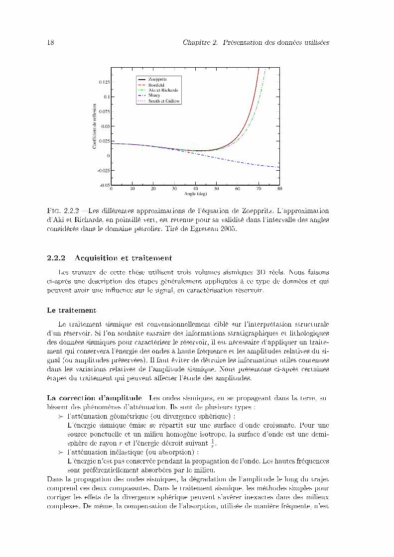
18 Chapitre 2. Présentation des données utilisées
Fig. 2.2.2 � Les di�érentes approximations de l'équation de Zoeppritz. L'approximationd'Aki et Richards, en pointillé vert, est retenue pour sa validité dans l'intervalle des anglesconsidérés dans le domaine pétrolier. Tiré de Egreteau 2005.
2.2.2 Acquisition et traitementLes travaux de cette thèse utilisent trois volumes sismiques 3D réels. Nous faisons
ci-après une description des étapes généralement appliquées à ce type de données et quipeuvent avoir une in�uence sur le signal, en caractérisation réservoir.
Le traitementLe traitement sismique est conventionnellement ciblé sur l'interprétation structurale
d'un réservoir. Si l'on souhaite extraire des informations stratigraphiques et lithologiquesdes données sismiques pour caractériser le réservoir, il est nécessaire d'appliquer un traite-ment qui conservera l'énergie des ondes à haute fréquence et les amplitudes relatives du si-gnal (ou amplitudes préservées). Il faut éviter de détruire les informations utiles contenuesdans les variations relatives de l'amplitude sismique. Nous présentons ci-après certainesétapes du traitement qui peuvent a�ecter l'étude des amplitudes.
La correction d'amplitude Les ondes sismiques, en se propageant dans la terre, su-bissent des phénomènes d'atténuation. Ils sont de plusieurs types :
� l'atténuation géométrique (ou divergence sphérique) :L'énergie sismique émise se répartit sur une surface d'onde croissante. Pour unesource ponctuelle et un milieu homogène isotrope, la surface d'onde est une demi-sphère de rayon r et l'énergie décroît suivant 1
r .� l'atténuation inélastique (ou absorption) :
L'énergie n'est pas conservée pendant la propagation de l'onde. Les hautes fréquencessont préférentiellement absorbées par le milieu.
Dans la propagation des ondes sismiques, la dégradation de l'amplitude le long du trajetcomprend ces deux composantes. Dans le traitement sismique, les méthodes simples pourcorriger les e�ets de la divergence sphérique peuvent s'avérer inexactes dans des milieuxcomplexes. De même, la compensation de l'absorption, utilisée de manière fréquente, n'est
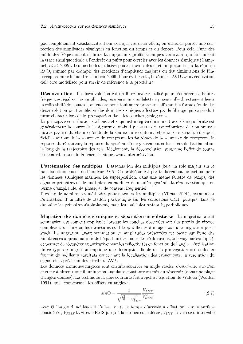
2.2. Avant-propos sur les données sismiques 19
pas complètement satisfaisante. Pour corriger ces deux e�ets, on utilisera plutôt une cor-rection des amplitudes sismiques en fonction du temps et du déport. Pour cela, l'une desméthodes fréquemment utilisées fait appel aux pro�ls sismiques verticaux, qui fournissentla trace sismique idéale à l'endroit du puits pour corréler avec les données sismiques (Camp-bell et al. 2005). Les méthodes utilisées peuvent avoir des e�ets importants sur la réponseAVO, comme par exemple des gradients d'amplitude majorés ou des diminutions de l'in-tercept comme le montre Cambois 2000. Pour éviter cela, la réponse AVO avant égalisationdoit être modélisée pour servir de référence à la procédure.Déconvolution La déconvolution est un �ltre inverse utilisé pour récupérer les hautesfréquences, égaliser les amplitudes, récupérer une ondelette à phase nulle directement liée àla ré�ectivité du sous-sol, ou encore pour tout autre processus a�ectant la forme d'onde. Ladéconvolution peut améliorer des données sismiques a�ectées par le �ltrage qui se produitnaturellement lors de la propagation dans les couches géologiques.La principale contribution de l'ondelette qui est intégrée dans une trace sismique brute estgénéralement la source de la signature, mais il y a aussi des contributions de nombreusesautres parties du champ d'onde de la source au récepteur, telles que les structures super-�cielles autour de la source et du récepteur, les fantômes de la source et du récepteur, laréponse du récepteur, la réponse du système d'enregistrement et les e�ets de l'atténuationle long de la trajectoire des rais. Idéalement, la déconvolution supprime l'e�et de toutesces contributions de la trace sismique avant interprétation.L'atténuation des multiples L'atténuation des multiples joue un rôle majeur sur lebon fonctionnement de l'analyse AVA. Ce problème est particulièrement important pourles données sismiques marines. La superposition, dans une même fenêtre de temps, dessignaux primaires et de multiples, va modi�er de manière générale la réponse sismique enterme d'amplitude, de phase, et de contenu fréquentiel.Il existe de nombreuses méthodes pour atténuer les multiples (Yilmaz 2001), notammentl'utilisation d'un �ltre de Radon parabolique sur les collections CMP puisque dans cedomaine les primaires s'aplatissent, mais les multiples restent hyperboliques.Migration des données sismiques et séparation en substacks La migration avantsommation est souvent appliquée lorsque les couches observées ont des pro�ls de vitessecomplexes, ou lorsque les structures sont trop di�ciles à imager par une migration post-stack. La migration avant sommation en amplitudes préservées est basée sur l'une desnombreuses approximations de l'équation des ondes (tracé de rayons, one-way par exemple),et permet de récupérer quantitativement les ré�ectivités en fonction de l'angle. L'utilisationde ce type de migration implique une description �able de la propagation des ondes etfournit de meilleurs résultats concernant la localisation des évènements, la résolution dusignal et la précision des attributs AVA.Les données sismiques migrées sont ensuite séparées en angle stacks, c'est-à-dire que l'oncherche à obtenir une illumination angulaire constante au toit du réservoir (dans une plaged'angles donnée). La technique la plus courante fait appel à l'équation de Walden (Walden1991), qui "transforme" les o�sets en angles :
sinΘ =x√
t20 + x2
V 2RMS
VINT
V 2RMS
(2.7)
avec Θ l'angle d'incidence à l'o�set x ; t0 le temps d'arrivée à o�set nul sur la surfaceconsidérée ; VRMS la vitesse RMS jusqu'à la surface considérée ; VINT la vitesse d'intervalle
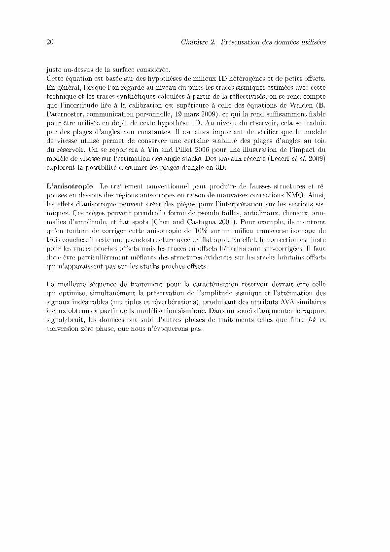
20 Chapitre 2. Présentation des données utilisées
juste au-dessus de la surface considérée.Cette équation est basée sur des hypothèses de milieux 1D hétérogènes et de petits o�sets.En général, lorsque l'on regarde au niveau du puits les traces sismiques estimées avec cettetechnique et les traces synthétiques calculées à partir de la ré�ectivités, on se rend compteque l'incertitude liée à la calibration est supérieure à celle des équations de Walden (B.Paternoster, communication personnelle, 19 mars 2009), ce qui la rend su�samment �ablepour être utilisée en dépit de cette hypothèse 1D. Au niveau du réservoir, cela se traduitpar des plages d'angles non constantes. Il est alors important de véri�er que le modèlede vitesse utilisé permet de conserver une certaine stabilité des plages d'angles au toitdu réservoir. On se reportera à Yin and Pillet 2006 pour une illustration de l'impact dumodèle de vitesse sur l'estimation des angle stacks. Des travaux récents (Lecerf et al. 2009)explorent la possibilité d'estimer les plages d'angle en 3D.
L'anisotropie Le traitement conventionnel peut produire de fausses structures et ré-ponses en-dessous des régions anisotropes en raison de mauvaises corrections NMO. Ainsi,les e�ets d'anisotropie peuvent créer des pièges pour l'interprétation sur les sections sis-miques. Ces pièges peuvent prendre la forme de pseudo failles, anticlinaux, chenaux, ano-malies d'amplitude, et �at spots (Chen and Castagna 2000). Pour exemple, ils montrentqu'en tentant de corriger cette anisotropie de 10% sur un milieu transverse isotrope detrois couches, il reste une pseudostructure avec un �at spot. En e�et, la correction est justepour les traces proches o�sets mais les traces en o�sets lointains sont sur-corrigées. Il fautdonc être particulièrement mé�ants des structures évidentes sur les stacks lointains o�setsqui n'apparaissent pas sur les stacks proches o�sets.La meilleure séquence de traitement pour la caractérisation réservoir devrait être cellequi optimise, simultanément la préservation de l'amplitude sismique et l'atténuation dessignaux indésirables (multiples et réverbérations), produisant des attributs AVA similairesà ceux obtenus à partir de la modélisation sismique. Dans un souci d'augmenter le rapportsignal/bruit, les données ont subi d'autres phases de traitements telles que �ltre f-k etconversion zéro phase, que nous n'évoquerons pas.

2.3. Le champ Alpha - modèle turbiditique 21
2.3 Le champ Alpha - modèle turbiditique
Fig. 2.3.1 � Localisation géographique du champ Alpha.
Le champ Alpha se situe au large des côtes angolaises dans le bassin du Congo inférieur,sur la marge continentale ouest africaine. On se trouve dans un contexte en eaux profondes(tranche d'eau de plus de 1500 mètres).
2.3.1 Le contexte géologiqueL'Angola est à cheval sur les trois bassins de sels majeurs de la marge atlantique de
l'Afrique. La région côtière du nord repose dans le bassin du Congo. Ce bassin est unestructure en pull-apart classique qui s'est développée sur la marge passive africaine pen-dant la rupture continentale du Crétacé.Une importante couche d'évaporites (sel) sépare deux séquences sédimentaires distinctes (lasérie pré-sel et la série post-sel). Les sédiments pré-sel ont été in�uencés structurellementpar une fracturation de la roche mère, associée à de la tectonique de raft. Les sédimentspost-sel ont été largement remaniés par des mouvements du sel sous-jacent. Ces deux sériessédimentaires sont riches en huile.L'évolution des bassins côtiers de l'Angola provient des événements de la tectonique desplaques qui a causé le rifting du supercontinent Gondwana et la séparation de l'Afriquede l'Amérique du sud. Le rifting a commencé au Crétacé Inférieur et un élargissementprogressif de l'Océan Atlantique Sud s'est amorcé. Après le début de cet élargissement, lesbassins de l'Angola, dont le bassin du Congo, ont continué à subsider, permettant le dépôtd'épais sédiments post-rift. L'évolution tectonique et sédimentaire de la marge angolaisepeut être divisée en huit phases séquentielles. La �gure 2.3.2 résume ces huit phases.Le champ Alpha s'est développé pendant les phases VI, VII et VIII, du Tertiaire Inférieurau Miocène Moyen. Ces phases sont constituées d'une grande proportion d'argiles et dequelques carbonates, re�étant l'ouverture continue de l'Atlantique. L'Oligocène a été unepériode de larges dépôts de turbidites. Les dépôts oligocènes sont essentiellement turbidi-tiques, avec des chenaux sableux intercalés. La formation Malembo, d'âge Oligocène, est

22 Chapitre 2. Présentation des données utilisées
une unité lithostratigraphique transgressive qui contient des strates formées proche littoralet en contexte de talus. Cette formation inclut certains des plus importants réservoirs dansles eaux profondes de l'Angola.La structure du champ Alpha, présenté en contexte régionale sur la �gure 2.3.3, est unanticlinal pincé en contexte compressif, initié à la fois par les mouvements salifères et parune déformation de glissements gravitaires. Cette structure, inclue dans la formation Ma-lembo, se forme pendant le déplacement gravitaire oligocène et se stabilise vers la �n duMiocène. L'unique puits dévié (W-Alpha) de la structure a été foré sur le �anc sud-ouestde l'anticlinal et traverse le �at spot des réservoirs oligocènes. Cette structure est a�ectéepar des failles d'extrados qui ne brisent pas la couverture.

2.3. Le champ Alpha - modèle turbiditique 23
Fig. 2.3.2 � Evolution stratigraphique des bassins o�shore angolais. De Brown�eld andCharpentier 2006b.
Fig. 2.3.3 � Interprétation géologique régionale du champ Alpha.
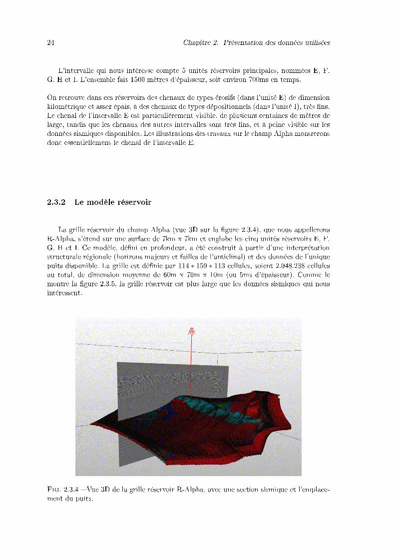
24 Chapitre 2. Présentation des données utilisées
L'intervalle qui nous intéresse compte 5 unités réservoirs principales, nommées E, F,G, H et I. L'ensemble fait 1500 mètres d'épaisseur, soit environ 700ms en temps.On retrouve dans ces réservoirs des chenaux de types érosifs (dans l'unité E) de dimensionkilométrique et assez épais, à des chenaux de types dépositionnels (dans l'unité I), très �ns.Le chenal de l'intervalle E est particulièrement visible, de plusieurs centaines de mètres delarge, tandis que les chenaux des autres intervalles sont très �ns, et à peine visible sur lesdonnées sismiques disponibles. Les illustrations des travaux sur le champ Alpha montrerontdonc essentiellement le chenal de l'intervalle E.
2.3.2 Le modèle réservoir
La grille réservoir du champ Alpha (vue 3D sur la �gure 2.3.4), que nous appelleronsR-Alpha, s'étend sur une surface de 7km x 7km et englobe les cinq unités réservoirs E, F,G, H et I. Ce modèle, dé�ni en profondeur, a été construit à partir d'une interprétationstructurale régionale (horizons majeurs et failles de l'anticlinal) et des données de l'uniquepuits disponible. La grille est dé�nie par 114 ∗ 159 ∗ 113 cellules, soient 2.048.238 cellulesau total, de dimension moyenne de 60m x 70m x 10m (ou 5ms d'épaisseur). Comme lemontre la �gure 2.3.5, la grille réservoir est plus large que les données sismiques qui nousintéressent.
Fig. 2.3.4 � Vue 3D de la grille réservoir R-Alpha, avec une section sismique et l'emplace-ment du puits.
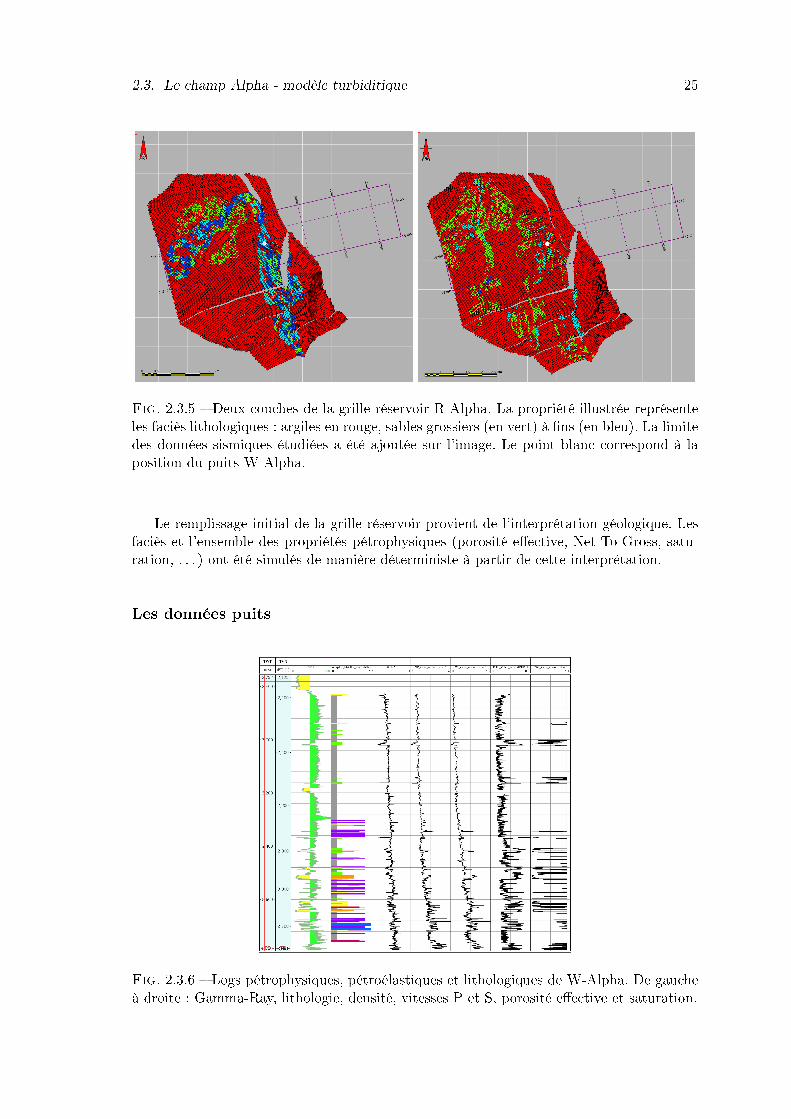
2.3. Le champ Alpha - modèle turbiditique 25
Fig. 2.3.5 � Deux couches de la grille réservoir R-Alpha. La propriété illustrée représenteles faciès lithologiques : argiles en rouge, sables grossiers (en vert) à �ns (en bleu). La limitedes données sismiques étudiées a été ajoutée sur l'image. Le point blanc correspond à laposition du puits W-Alpha.
Le remplissage initial de la grille réservoir provient de l'interprétation géologique. Lesfaciès et l'ensemble des propriétés pétrophysiques (porosité e�ective, Net-To-Gross, satu-ration, . . . ) ont été simulés de manière déterministe à partir de cette interprétation.
Les données puits
Fig. 2.3.6 � Logs pétrophysiques, pétroélastiques et lithologiques de W-Alpha. De gaucheà droite : Gamma-Ray, lithologie, densité, vitesses P et S, porosité e�ective et saturation.
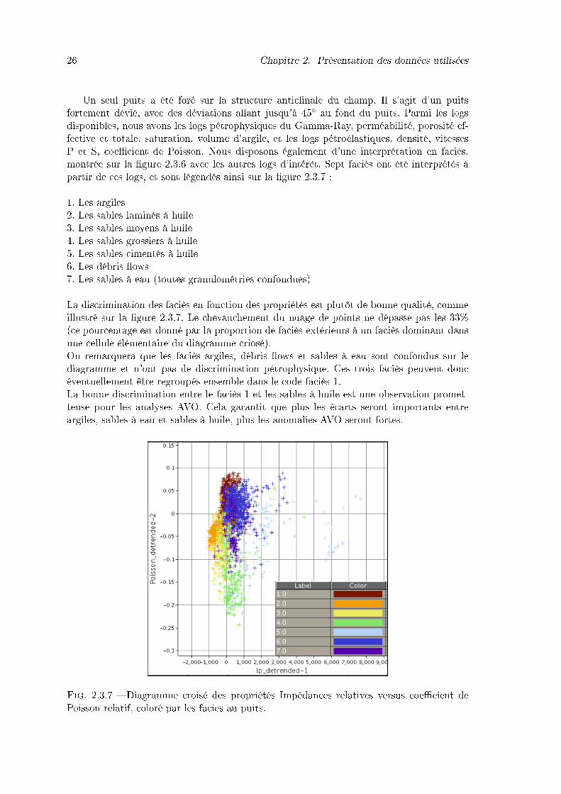
26 Chapitre 2. Présentation des données utilisées
Un seul puits a été foré sur la structure anticlinale du champ. Il s'agit d'un puitsfortement dévié, avec des déviations allant jusqu'à 45◦ au fond du puits. Parmi les logsdisponibles, nous avons les logs pétrophysiques du Gamma-Ray, perméabilité, porosité ef-fective et totale, saturation, volume d'argile, et les logs pétroélastiques, densité, vitessesP et S, coe�cient de Poisson. Nous disposons également d'une interprétation en faciès,montrée sur la �gure 2.3.6 avec les autres logs d'intérêt. Sept faciès ont été interprétés àpartir de ces logs, et sont légendés ainsi sur la �gure 2.3.7 :1. Les argiles2. Les sables laminés à huile3. Les sables moyens à huile4. Les sables grossiers à huile5. Les sables cimentés à huile6. Les débris �ows7. Les sables à eau (toutes granulométries confondues)La discrimination des faciès en fonction des propriétés est plutôt de bonne qualité, commeillustré sur la �gure 2.3.7. Le chevauchement du nuage de points ne dépasse pas les 33%(ce pourcentage est donné par la proportion de faciès extérieurs à un faciès dominant dansune cellule élémentaire du diagramme criosé).On remarquera que les faciès argiles, débris �ows et sables à eau sont confondus sur lediagramme et n'ont pas de discrimination pétrophysique. Ces trois faciès peuvent doncéventuellement être regroupés ensemble dans le code faciès 1.La bonne discrimination entre le faciès 1 et les sables à huile est une observation promet-teuse pour les analyses AVO. Cela garantit que plus les écarts seront importants entreargiles, sables à eau et sables à huile, plus les anomalies AVO seront fortes.
Fig. 2.3.7 � Diagramme croisé des propriétés Impédances relatives versus coe�cient dePoisson relatif, coloré par les facies au puits.

2.3. Le champ Alpha - modèle turbiditique 27
Un modèle pétroélastique (PEM) a été dé�ni à partir de W-Alpha, pour reconstituerles propriétés densité ρ, vitesse P Vp et vitesse S Vs à partir des faciès et des courbesd'enfouissement {ρ, Vp, Vs} = f(z). Pour stabiliser les relations issues de ces courbes d'en-fouissement, les propriétés d'un puits du champ voisin (distant de 12 Km) ont été ajoutéesà celles de W-Alpha. La �gure 2.3.8 montre les données de puits pour la densité, les vitessesP et S, avec les courbes d'enfouissement.
Fig. 2.3.8 � Courbes d'enfouissement estimées pour le puits W-Alpha, pour les propriétésdensité, vitesses P et S. Les points rouges correspondent aux données du puits W-Alpha,les points verts aux données du puits voisin.
2.3.3 Les données sismiques
Il s'agit d'un bloc 3D de données sismiques marines acquises avec une tranche d'eaud'environ 1500m. Les caractéristiques principales de la zone étudiée sont les suivantes :
� Echantillonnage spatial : 12.50m x 12.50m� Dimension : 151 Inlines x 661 crosslines x 1668 échantillons (tmin = 1500ms)� Pas d'échantillonnage en temps : 3ms� Fréquence dominante : 30 Hz (résolution de 21m)� Bande passante : 5 - 100 Hz
Trois substacks (Near stack 5◦-18◦, mid stack 18◦-32◦ et far stack 32◦-47◦) ont été créés àpartir de cette acquisition. La �gure 2.3.9 montre une section de la sismique Near suivantles directions inline et crossline. Le réservoir est individualisé par les horizons bleus.
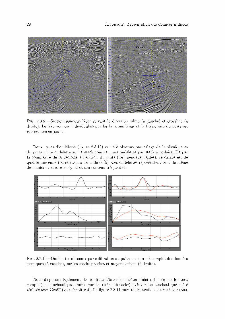
28 Chapitre 2. Présentation des données utilisées
Fig. 2.3.9 � Section sismique Near suivant la direction inline (à gauche) et crossline (àdroite). Le réservoir est individualisé par les horizons bleus et la trajectoire du puits estreprésentée en jaune.
Deux types d'ondelette (�gure 2.3.10) ont été obtenus par calage de la sismique etdu puits : une ondelette sur le stack complet, une ondelette par stack angulaire. De parla complexité de la géologie à l'endroit du puits (fort pendage, failles), ce calage est dequalité moyenne (corrélation autour de 60%). Ces ondelettes représentent tout de mêmede manière correcte le signal et son contenu fréquentiel.
Fig. 2.3.10 � Ondelettes obtenues par calibration au puits sur le stack complet des donnéessismiques (à gauche), sur les stacks proches et moyens o�sets (à droite).
Nous disposons également de résultats d'inversions déterministes (basée sur le stackcomplet) et stochastiques (basée sur les trois substacks). L'inversion stochastique a étéréalisée avec GeoSI (voir chapitre 4). La �gure 2.3.11 montre des sections de ces inversions,

2.3. Le champ Alpha - modèle turbiditique 29
en impédances P et S, pour les deux types d'inversions. La di�érence principale, outre ladi�érence de valeurs des impédances, est le niveau de détail, la résolution de ces résultats.En e�et, l'inversion stochastique a une résolution verticale plus �ne, ce qui peut permettrede simuler d'autres propriétés avec plus d'hétérogénéités que dans le cas de l'inversiondéterministe. De plus, les impédances stochastiques sont échantillonnées à 1ms.
Fig. 2.3.11 � Sections en impedances P (à gauche) et S (à droite) pour les inversionsdeterministes (en haut) et stochastiques (en bas). L'inversion stochastique est réalisée uni-quement sur le réservoir R-Alpha.
2.3.4 Les particularités du champ AlphaLe champ Alpha a l'avantage certain d'une sismique 3D avec un excellent rapport
signal/bruit.Un seul puits au sommet de la structure anticlinale permet de contraindre cette sismiqueavec des propriétés pétrophysiques. Le seul PEM existant se base sur ce puits, et est formuléà partir des courbes d'enfouissement des propriétés pétroélastiques et de l'interprétationen faciès du puits. Ce PEM est donc peu �able sur l'ensemble du champ, étant donné lefort pendage de la structure (environ 40◦). Il est donc peu probable que les informationsactuelles de la grille réservoir nous permettent de retrouver les données sismiques réelles.
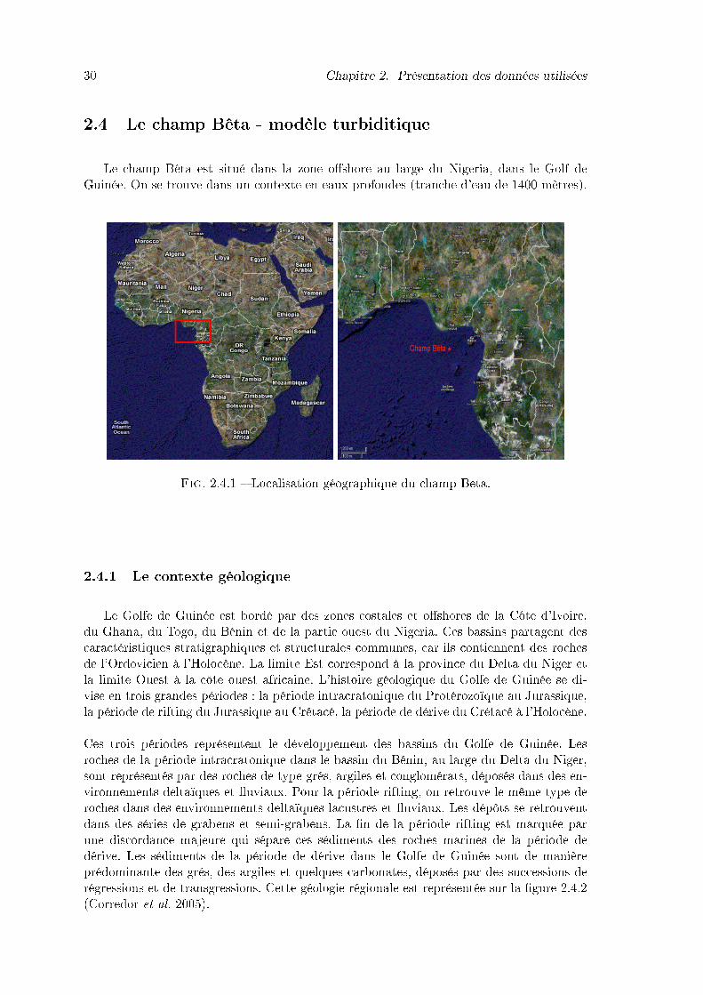
30 Chapitre 2. Présentation des données utilisées
2.4 Le champ Bêta - modèle turbiditique
Le champ Bêta est situé dans la zone o�shore au large du Nigeria, dans le Golf deGuinée. On se trouve dans un contexte en eaux profondes (tranche d'eau de 1400 mètres).
Fig. 2.4.1 � Localisation géographique du champ Beta.
2.4.1 Le contexte géologique
Le Golfe de Guinée est bordé par des zones costales et o�shores de la Côte d'Ivoire,du Ghana, du Togo, du Bénin et de la partie ouest du Nigeria. Ces bassins partagent descaractéristiques stratigraphiques et structurales communes, car ils contiennent des rochesde l'Ordovicien à l'Holocène. La limite Est correspond à la province du Delta du Niger etla limite Ouest à la côte ouest africaine. L'histoire géologique du Golfe de Guinée se di-vise en trois grandes périodes : la période intracratonique du Protérozoïque au Jurassique,la période de rifting du Jurassique au Crétacé, la période de dérive du Crétacé à l'Holocène.Ces trois périodes représentent le développement des bassins du Golfe de Guinée. Lesroches de la période intracratonique dans le bassin du Bénin, au large du Delta du Niger,sont représentés par des roches de type grés, argiles et conglomérats, déposés dans des en-vironnements deltaïques et �uviaux. Pour la période rifting, on retrouve le même type deroches dans des environnements deltaïques lacustres et �uviaux. Les dépôts se retrouventdans des séries de grabens et semi-grabens. La �n de la période rifting est marquée parune discordance majeure qui sépare ces sédiments des roches marines de la période dedérive. Les sédiments de la période de dérive dans le Golfe de Guinée sont de manièreprédominante des grés, des argiles et quelques carbonates, déposés par des successions derégressions et de transgressions. Cette géologie régionale est représentée sur la �gure 2.4.2(Corredor et al. 2005).
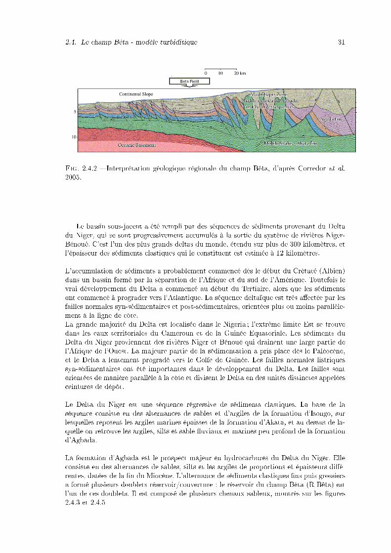
2.4. Le champ Bêta - modèle turbiditique 31
Fig. 2.4.2 � Interprétation géologique régionale du champ Bêta, d'après Corredor et al.2005.
Le bassin sous-jacent a été rempli par des séquences de sédiments provenant du Deltadu Niger, qui se sont progressivement accumulés à la sortie du système de rivières Niger-Bénoué. C'est l'un des plus grands deltas du monde, étendu sur plus de 300 kilomètres, etl'épaisseur des sédiments clastiques qui le constituent est estimée à 12 kilomètres.L'accumulation de sédiments a probablement commencé dès le début du Crétacé (Albien)dans un bassin formé par la séparation de l'Afrique et du sud de l'Amérique. Toutefois levrai développement du Delta a commencé au début du Tertiaire, alors que les sédimentsont commencé à prograder vers l'Atlantique. La séquence deltaïque est très a�ectée par lesfailles normales syn-sédimentaires et post-sédimentaires, orientées plus ou moins parallèle-ment à la ligne de côte.La grande majorité du Delta est localisée dans le Nigeria ; l'extrême limite Est se trouvedans les eaux territoriales du Cameroun et de la Guinée Equatoriale. Les sédiments duDelta du Niger proviennent des rivières Niger et Bénoué qui drainent une large partie del'Afrique de l'Ouest. La majeure partie de la sédimentation a pris place dès le Paléocène,et le Delta a lentement progradé vers le Golfe de Guinée. Les failles normales listriquessyn-sédimentaires ont été importantes dans le développement du Delta. Les failles sontorientées de manière parallèle à la côte et divisent le Delta en des unités distinctes appeléesceintures de dépôt.Le Delta du Niger est une séquence régressive de sédiments clastiques. La base de laséquence consiste en des alternances de sables et d'argiles de la formation d'Isongo, surlesquelles reposent les argiles marines épaisses de la formation d'Akata, et au dessus de la-quelle on retrouve les argiles, silts et sable �uviaux et marines peu profond de la formationd'Agbada.La formation d'Agbada est le prospect majeur en hydrocarbures du Delta du Niger. Elleconsiste en des alternances de sables, silts et les argiles de proportions et épaisseurs di�é-rentes, datées de la �n du Miocène. L'alternance de sédiments clastiques �ns puis grossiersa formé plusieurs doublets réservoir/couverture : le réservoir du champ Bêta (R-Bêta) estl'un de ces doublets. Il est composé de plusieurs chenaux sableux, montrés sur les �gures2.4.3 et 2.4.5
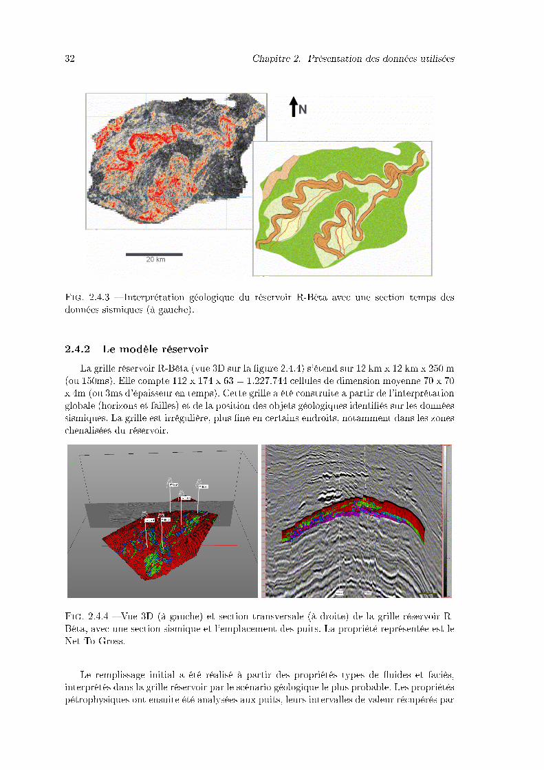
32 Chapitre 2. Présentation des données utilisées
Fig. 2.4.3 � Interprétation géologique du réservoir R-Bêta avec une section temps desdonnées sismiques (à gauche).
2.4.2 Le modèle réservoirLa grille réservoir R-Bêta (vue 3D sur la �gure 2.4.4) s'étend sur 12 km x 12 km x 250 m
(ou 150ms). Elle compte 112 x 174 x 63 = 1.227.744 cellules de dimension moyenne 70 x 70x 4m (ou 3ms d'épaisseur en temps). Cette grille a été construite a partir de l'interprétationglobale (horizons et failles) et de la position des objets géologiques identi�és sur les donnéessismiques. La grille est irrégulière, plus �ne en certains endroits, notamment dans les zoneschenalisées du réservoir.
Fig. 2.4.4 � Vue 3D (à gauche) et section transversale (à droite) de la grille réservoir R-Bêta, avec une section sismique et l'emplacement des puits. La propriété représentée est leNet-To-Gross.
Le remplissage initial a été réalisé à partir des propriétés types de �uides et faciès,interprétés dans la grille réservoir par le scénario géologique le plus probable. Les propriétéspétrophysiques ont ensuite été analysées aux puits, leurs intervalles de valeur récupérés par
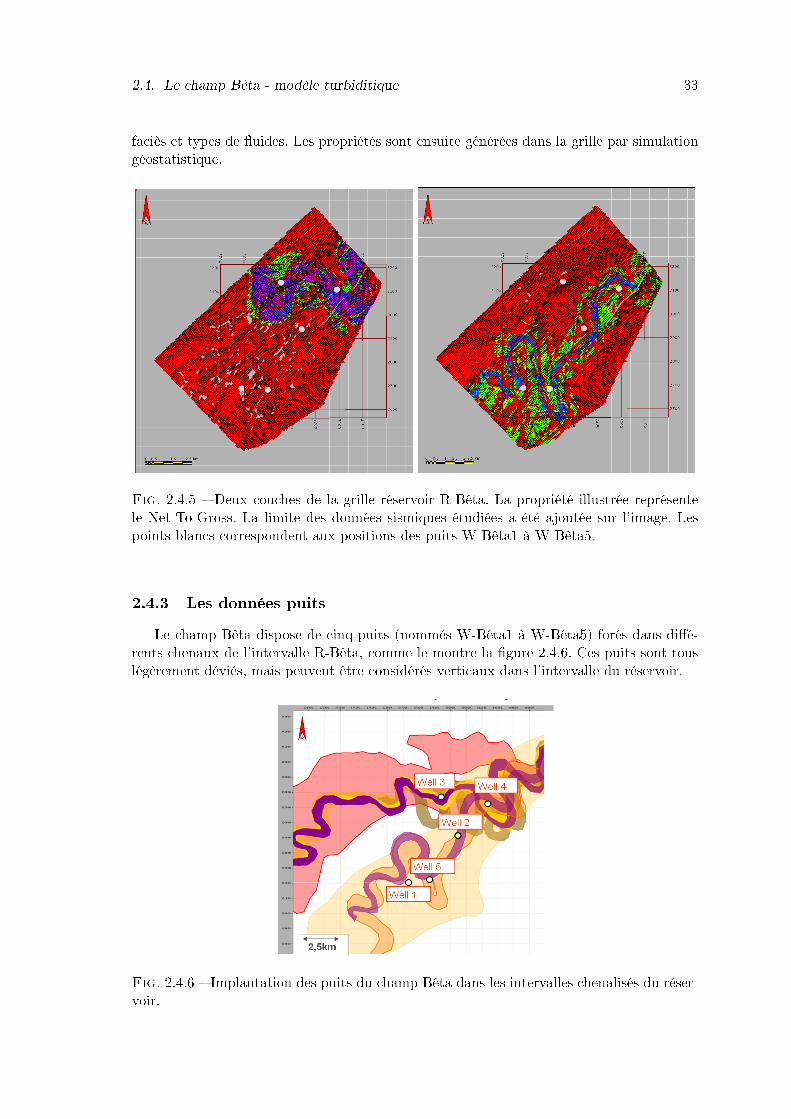
2.4. Le champ Bêta - modèle turbiditique 33
faciès et types de �uides. Les propriétés sont ensuite générées dans la grille par simulationgéostatistique.
Fig. 2.4.5 � Deux couches de la grille réservoir R-Bêta. La propriété illustrée représentele Net-To-Gross. La limite des données sismiques étudiées a été ajoutée sur l'image. Lespoints blancs correspondent aux positions des puits W-Bêta1 à W-Bêta5.
2.4.3 Les données puitsLe champ Bêta dispose de cinq puits (nommés W-Bêta1 à W-Bêta5) forés dans di�é-
rents chenaux de l'intervalle R-Bêta, comme le montre la �gure 2.4.6. Ces puits sont touslégèrement déviés, mais peuvent être considérés verticaux dans l'intervalle du réservoir.
Fig. 2.4.6 � Implantation des puits du champ Bêta dans les intervalles chenalisés du réser-voir.

34 Chapitre 2. Présentation des données utilisées
Parmi les logs disponibles, nous avons les logs pétrophysiques du Gamma-Ray, perméa-bilité, porosité e�ective et totale, saturation, volume d'argile, et les logs pétroélastiques,densité, vitesses P et S, coe�cient de Poisson. Nous disposons également d'une interpréta-tion en faciès, montrée sur la �gure 2.4.7 avec les autres logs d'intérêt. Les faciès interprétéssont légendés ainsi :1. Argiles silteuses2. Argiles turbiditiques avec laminations sableuses très �nes3. Silts et sables �ns en bancs alternés centimétriques4. Silts et sables �ns en bancs alternés décimétriques5. Sables moyens6. Sables grossiers à graveleux7. Matrice argileuse à quartz8. Matrice sablo-argileuse à quartz9. Sables �ns en bancs massifs décimétriques10. Sables moyens en bancs massifs plurimétriques11. Niveau conglomératique de base de chenal ou Lag12. Sills ou dykes sableux métriques
Fig. 2.4.7 � Logs lithologiques et pétroélastiques (lithologie, densité, vitesses P et S) pourles cinq puits du champ Bêta.
La discrimination des faciès en fonction des propriétés est assez di�cile, avec un chevau-chement entre 41% et 52% (en fonction du puits), comme illustré sur la �gure 2.4.8. Ceciest dû au fait que la réponse d'un faciès varie légèrement de puits à puits et d'intervalle enintervalle.
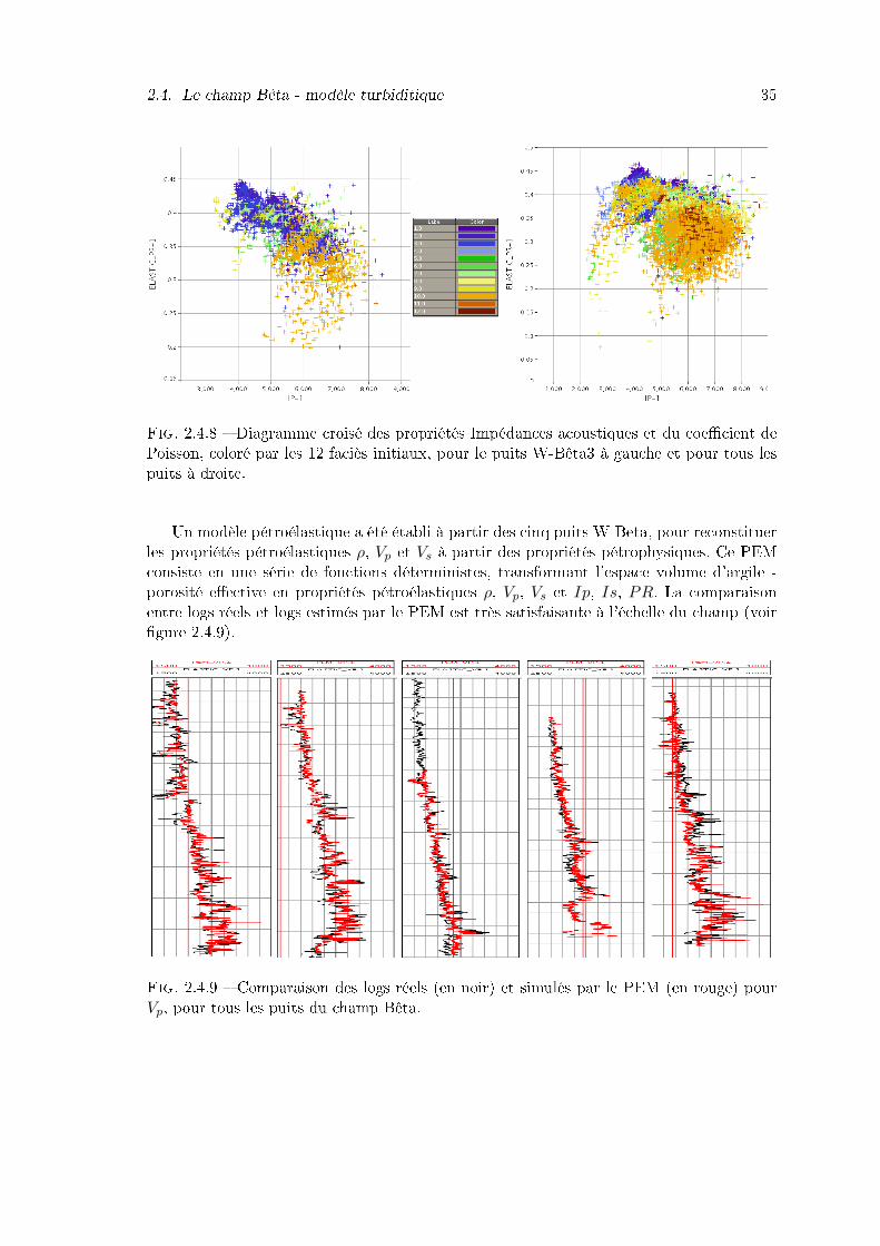
2.4. Le champ Bêta - modèle turbiditique 35
Fig. 2.4.8 � Diagramme croisé des propriétés Impédances acoustiques et du coe�cient dePoisson, coloré par les 12 faciès initiaux, pour le puits W-Bêta3 à gauche et pour tous lespuits à droite.
Un modèle pétroélastique a été établi à partir des cinq puits W-Beta, pour reconstituerles propriétés pétroélastiques ρ, Vp et Vs à partir des propriétés pétrophysiques. Ce PEMconsiste en une série de fonctions déterministes, transformant l'espace volume d'argile -porosité e�ective en propriétés pétroélastiques ρ, Vp, Vs et Ip, Is, PR. La comparaisonentre logs réels et logs estimés par le PEM est très satisfaisante à l'échelle du champ (voir�gure 2.4.9).
Fig. 2.4.9 � Comparaison des logs réels (en noir) et simulés par le PEM (en rouge) pourVp, pour tous les puits du champ Bêta.
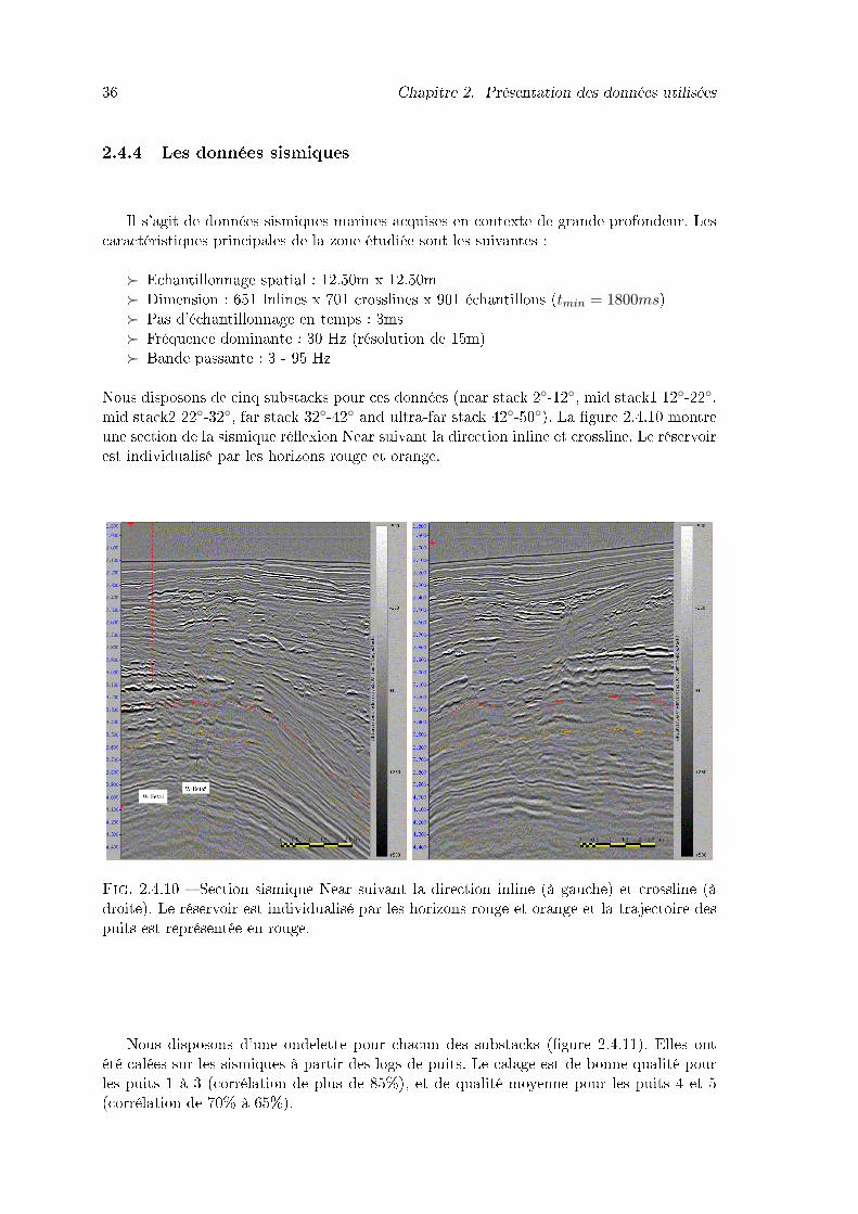
36 Chapitre 2. Présentation des données utilisées
2.4.4 Les données sismiques
Il s'agit de données sismiques marines acquises en contexte de grande profondeur. Lescaractéristiques principales de la zone étudiée sont les suivantes :
� Echantillonnage spatial : 12.50m x 12.50m� Dimension : 651 Inlines x 701 crosslines x 901 échantillons (tmin = 1800ms)� Pas d'échantillonnage en temps : 3ms� Fréquence dominante : 30 Hz (résolution de 15m)� Bande passante : 3 - 95 Hz
Nous disposons de cinq substacks pour ces données (near stack 2◦-12◦, mid stack1 12◦-22◦,mid stack2 22◦-32◦, far stack 32◦-42◦ and ultra-far stack 42◦-50◦). La �gure 2.4.10 montreune section de la sismique ré�exion Near suivant la direction inline et crossline. Le réservoirest individualisé par les horizons rouge et orange.
Fig. 2.4.10 � Section sismique Near suivant la direction inline (à gauche) et crossline (àdroite). Le réservoir est individualisé par les horizons rouge et orange et la trajectoire despuits est représentée en rouge.
Nous disposons d'une ondelette pour chacun des substacks (�gure 2.4.11). Elles ontété calées sur les sismiques à partir des logs de puits. Le calage est de bonne qualité pourles puits 1 à 3 (corrélation de plus de 85%), et de qualité moyenne pour les puits 4 et 5(corrélation de 70% à 65%).
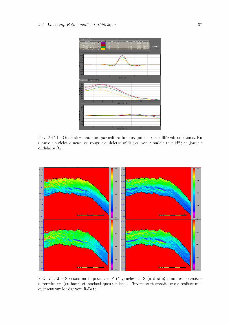
2.4. Le champ Bêta - modèle turbiditique 37
Fig. 2.4.11 � Ondelettes obtenues par calibration aux puits sur les di�érents substacks. Enmauve : ondelette near ; en rouge : ondelette mid1 ; en vert : ondelette mid2 ; en jaune :ondelette far.
Fig. 2.4.12 � Sections en impedances P (à gauche) et S (à droite) pour les inversionsdeterministes (en haut) et stochastiques (en bas). L'inversion stochastique est réalisée uni-quement sur le réservoir R-Bêta.
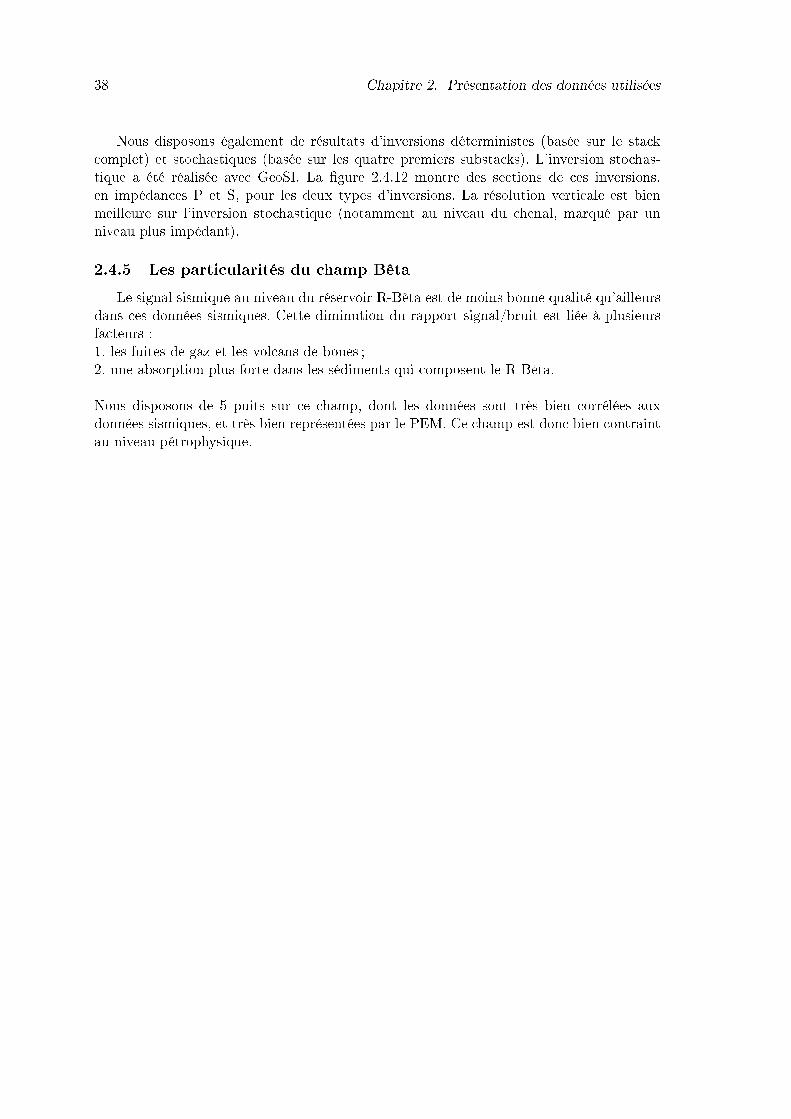
38 Chapitre 2. Présentation des données utilisées
Nous disposons également de résultats d'inversions déterministes (basée sur le stackcomplet) et stochastiques (basée sur les quatre premiers substacks). L'inversion stochas-tique a été réalisée avec GeoSI. La �gure 2.4.12 montre des sections de ces inversions,en impédances P et S, pour les deux types d'inversions. La résolution verticale est bienmeilleure sur l'inversion stochastique (notamment au niveau du chenal, marqué par unniveau plus impédant).
2.4.5 Les particularités du champ BêtaLe signal sismique au niveau du réservoir R-Bêta est de moins bonne qualité qu'ailleurs
dans ces données sismiques. Cette diminution du rapport signal/bruit est liée à plusieursfacteurs :1. les fuites de gaz et les volcans de boues ;2. une absorption plus forte dans les sédiments qui composent le R-Bêta.Nous disposons de 5 puits sur ce champ, dont les données sont très bien corrélées auxdonnées sismiques, et très bien représentées par le PEM. Ce champ est donc bien contraintau niveau pétrophysique.
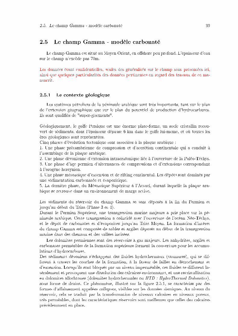
2.5. Le champ Gamma - modèle carbonaté 39
2.5 Le champ Gamma - modèle carbonatéLe champ Gamma est situé au Moyen Orient, en o�shore peu profond. L'épaisseur d'eau
sur le champ n'excède pas 70m.Les données étant con�dentielles, seules des généralités sur le champ sont présentées ici,ainsi que quelques particularités des données pertinentes en regard des travaux de ce ma-nuscrit.
2.5.1 Le contexte géologiqueLes systèmes pétroliers de la péninsule arabique sont très importants, tant sur le plan
de l'extension géographique que sur le plan du potentiel de production d'hydrocarbures.Ils sont quali�és de "super-gisements".Géologiquement, le golfe Persique est une énorme plate-forme, un socle cristallin recou-vert de sédiments, dont l'épaisseur dépasse 6 km dans le golfe lui-même, et où toutes lesères géologiques sont représentées.Cinq phases d'évolution tectonique sont associées à la plaque arabique :1. Une phase précambrienne de compression et d'accrétion continentale qui a conduit àl'assemblage de la plaque arabique.2. Une phase dévonienne d'extension intracratonique liée à l'ouverture de la Paléo-Téthys.3. Une phase d'âge permien d'alternances de compressions et d'extensions correspondantà l'orogène hercynien.4. Une phase mésozoique d'extension et de rifting continental. Les dépôts sont dominés parune sédimentation carbonatée et évaporitique.5. La dernière phase, du Mésozoique Supérieur à l'Actuel, durant laquelle la plaque ara-bique se retrouve dans un environnement de marge active.Les sédiments du réservoir du champ Gamma se sont déposés à la �n du Permien etjusqu'au début du Trias (Phase 3 et 4).Durant le Permien Supérieur, une transgression marine majeure a pris place sur la pé-ninsule arabique. Cette transgression a coïncidé avec l'ouverture de l'océan Néo-Téthys,et le dépôt de carbonates et d'évaporites jusqu'au Trias Moyen. La formation d'intérêtdu champ Gamma est composée de sables et argiles déposés au début de la transgressionmarine dans des chenaux et des vallées incisées.
Les dolomites permiennes sont des réservoirs à gaz majeurs. Les anhydrites, argiles etcarbonates perméables de la formation supérieure forment la couverture pour les accumu-lations d'hydrocarbures.Des sédiments dévoniens s'échappent des �uides hydrothermaux (saumures), qui se dif-fusent à travers les couches de la formation, à la faveur de failles en décrochement etd'extension. Lorsqu'ils sont bloqués par un niveau imperméable, ces �uides se di�usent la-téralement et provoquent une dissolution des calcaires environnants, et une recristallisationen dolomites allochtones (dolomites hydrothermales ou HTD : HydroThermal Dolomites),sous forme de drains. Ce phénomène, illustré sur la �gure 2.5.1, se caractérise par desformes d'a�aissement appelées collapses, visibles sur les données sismiques. Au niveau duréservoir, cela se traduit par la transformation de niveaux calcaires en niveaux poreux,très perméables, dont les caractéristiques réservoirs sont meilleures que celles des calcairesprécédemment en place.
40 Chapitre 2. Présentation des données utilisées
Fig. 2.5.1 � Principes de la dolomitisation hydrothermale dans les niveaux non perméablesdu réservoir Gamma.
2.5.2 Les particularités du champ GammaLes données de puits : Les logs des di�érents puits du champ montrent que les varia-tions des propriétés pétrophysiques sont très faibles. En e�et, d'un puits à un autre les logsd'une propriété donnée montrent de fortes similitudes.Trois grands faciès peuvent être identi�és sur ces données : anhydrites, calcaires et dolo-mites.
Les données sismiques : Il s'agit de données sismiques marines acquises en eaux peuprofondes (70 mètres maximum). On observe une importante di�érence de contenu fréquen-tiel et résolution entre les di�érents substacks. La sismique proche o�set est très bruitéeet a�ectée par des multiples internes, notamment sur l'intervalle juste au-dessus du réser-voir d'intérêt. La sismique lointain o�set, très basse fréquence, n'a plus les multiples. Lasismique intermédiaire est un compromis entre altération par les multiples et qualité dusignal.La qualité moyenne de la calibration puits-sismique (75% au mieux) est un frein pour l'in-tégration de l'information sismique dans le réservoir. Il faudra donc rester prudent sur lesrésultats des travaux qui feront intervenir les ondelettes.

Partie I
Validité de la grille réservoir
41


Chapitre 3
Modélisation sismique à partir de la grilleréservoir
3.1 IntroductionDans le domaine pétrolier, un soin particulier est apporté à la réalisation du modèle
géologique tout d'abord, puis à la réalisation du modèle réservoir. Ce dernier est le sup-port principal de l'information puisqu'il est ensuite utilisé comme donnée d'entrée dansdes simulateurs sophistiqués, a�n de simuler et prédire le comportement du réservoir lorsde son exploitation (Enge et al. 2007). Ces simulateurs faisant appel à des méthodes nu-mériques très complexes et étant très coûteux tant en mémoire qu'en temps de calcul, uneapproche essai-erreur sur les propriétés du réservoir est préjudiciable. En e�et, les erreurspeuvent provenir des propriétés statiques et/ou des propriétés dynamiques. Pour permettreune meilleure intégration, nous proposons une approche complémentaire : la modélisationsismique comme méthode de validation du modèle réservoir. Ainsi, nous pouvons validerles propriétés statiques en regard de la sismique, et donc diminuer leurs incertitudes. Lorsde la phase de simulation dynamique du réservoir, les erreurs seront donc essentiellementprovoquées par les incertitudes sur les propriétés dynamiques.La modélisation sismique est un processus de calcul par lequel un modèle géologique esttransformé en un enregistrement sismique synthétique. Si l'on considère l'utilité de la modé-lisation sismique, seule, sans faire référence à la grille réservoir, les enregistrements synthé-tiques générés par ce processus ont plusieurs vocations et utilités au cours de l'explorationd'un champ pétrolier et sont souvent générés avant et après l'acquisition des données desismique de ré�exion. Les sismiques synthétiques générés avant acquisition sont typique-ment utilisées pour ajuster les paramètres de l'acquisition (géométrie, nombre de sourceset de récepteurs, . . . ), a�n d'assurer que l'objectif géologique sera imagé et interprétablesur les données après traitement.Quand ces volumes synthétiques sont générés après l'acquisition, l'interprétateur cherchegénéralement à déterminer les caractéristiques des roches et des �uides, qui sont à l'originedes évènements observés sur les données sismiques réelles.La modélisation sismique devient alors une aide à l'interprétation (Breton et al. 2007).La di�érence entre données réelles et synthétiques permet de mettre en évidence les er-reurs du modèle réservoir, qu'il faut alors corriger, tout en maintenant la cohérence avecles autres types de données (puits, carottes, . . . ) qui servent de contraintes au modèle.Toutefois, ces comparaisons sont réalisées avec plus ou moins de pertinence. Pour que levolume synthétique soit aussi proche des données réelles que possible, il faut connaître lesstructures géologiques, leurs propriétés, mais aussi le signal sismique. Le choix de l'onde-
43
44 Chapitre 3. Modélisation sismique à partir de la grille réservoir
lette, qui représente la forme du signal à modéliser, est essentiel pour reproduire le contenufréquentiel et la phase du signal sismique.Le support du modèle réservoir est une grille irrégulière en espace. On peut simuler di-rectement un volume sismique régulièrement échantillonné à partir d'une grille réservoir,mais cela passe par l'utilisation de méthodes complexes et di�ciles à mettre en oeuvre.Pour que la modélisation sismique sur grille réservoir soit facile et rapide à mettre enoeuvre, nous créons un support intermédiaire entre données sismiques et modèle réservoir.Ce chapitre présente la procédure de modélisation sismique à partir d'un modèle réser-voir. Cette modélisation permettra de faire le lien entre les simulateurs réservoir ou lesgéomodeleurs et la réponse sismique du réservoir.
3.2 Calcul des données sismiques synthétiquesIl existe une multitude de méthodes permettant de créer un volume sismique synthé-
tique à partir de propriétés élastiques. Carcione (Carcione et al. 2002) et Krebes (Krebes2004) font un état de l'art des méthodes existantes en modélisation sismique, dont voici unrapide résumé.
3.2.1 Le modèle convolutionnel 1DIl s'agit de la méthode la plus ancienne, la plus simple et la plus utilisée dans le domaine
de la modélisation sismique. Cette méthode de modélisation est la première réalisée surune étude, dès que des puits ont été forés et les logs soniques enregistrés. Sa formulation estbasée sur la création d'une trace sismique s par la convolution d'une ondelette w (la formed'onde de la source sismique) et de la ré�ectivité R (la série de coe�cients de ré�exionreplacés en temps de trajet t).
s(t) = R(t)⊗ w(t) (3.1)Ou sous sa forme continue :
s(t) =∫ ∞
−∞w(τ) ∗R(t− τ)dτ (3.2)
Si w(t) et R(t) sont des fonctions discrétisées, on aura :
s(k) =n+k∑n=0
w(k) ∗R(k − n) (3.3)
La trace sismique est le résultat de la convolution de la forme d'onde de la source avecla réponse impulsive de la Terre. Cette réponse impulsive contient certes la ré�ectivité,mais aussi les multiples, les ondes converties et les e�ets d'atténuation, entre autres. Lamodélisation par convolution simule donc des données sismiques idéalement traitées. Lapropagation des ondes sismiques n'y est pas simulée, ni ses e�ets sur le sismogramme enre-gistré, puisque cette approche est basée sur l'hypothèse que l'onde est plane. La générationde sismogrammes synthétiques par modèle convolutionnel est donc incomplète du point devue physique mais est très utile dans de nombreux contextes.Par exemple, On l'utilise si nous voulons construire un sismogramme à comparer à desimages sismiques �nales. Dans ce cas, nous avons supprimés les multiples et corrigés l'atté-nuation. Une autre application utile, est de considérer que le modèle convolutif s'applique

3.2. Calcul des données sismiques synthétiques 45
dans une petite fenêtre de temps, où l'on entend par ondelette la source après sa modi�-cation par l'atténuation et les multiples au-dessus de la fenêtre.La qualité du sismogramme synthétique en regard de la trace sismique correspondantedépend entre autres de la qualité des logs (qu'ils proviennent des puits ou de modèles), dutraitement des données sismiques et de la capacité à extraire une ondelette sismique repré-sentative de la donnée sismique. L'ondelette source n'est généralement pas connue, maisestimée à partir des données par des techniques de calibration (Ziolkowski et al. 1998, Linari2004).Quant aux ré�ectivités, elles seront calculées à partir des logs de vitesse, en utilisantles relations pour les ré�ectivités à incidence nulle (voir équation 2.2), et l'approximationde Aki and Richards 1980 pour les incidences non nulles (voir équation 2.6).
3.2.2 Le tracé de rayonsAu passage des ondes sismiques, les particules du sous-sol se mettent en mouvement.
La surface sur laquelle les déplacements sont en phase à un instant donné est par dé�nitionle front d'onde ; les normales aux fronts d'ondes en milieu isotrope sont les rayons sismiquesou rais. La théorie des rais (Cerveny 2001) permet de calculer l'énergie de l'onde suivantla trajectoire des rais plutôt que celle des fronts d'ondes.Dans la modélisation par tracé de rayons (Virieux and Farra 1991), on fait une approxi-mation haute fréquence de la solution exacte de l'équation d'onde. Cette approximationrepose sur plusieurs hypothèses :
� Le champ de vitesse du réservoir varie à plus basse fréquence que l'onde sismique(sa longueur d'onde est plus grande que celle de l'onde).
� L'onde est supposée plane.� La direction de propagation suit la loi de Snell-Descartes.
Ces simpli�cations font du tracé de rayons un bon candidat pour simuler rapidement un vo-lume sismique synthétique à partir d'un modèle "basse fréquence". Ces méthodes sont trèsutilisées pour l'interprétation structurale mais peu indiquées pour faire de la caractérisationréservoir.
3.2.3 Modélisation numérique de l'équation des ondesDi�érentes méthodes numériques ont été développées pour résoudre l'équation des ondes
dans des milieux complexes et avec des conditions aux limites sophistiquées. Parmi lespremières méthodes, Virieux 1986 utilisent la méthode des di�érences �nies, qui comptede nombreuses variantes. La propagation de la forme d'onde est identi�ée dès son point dedépart comme une onde complète, et le modèle géologique est caractérisé par sa densitéet sa compressibilité (dans le cas acoustique), ou par son module de cisaillement (casélastique). Les ondes se propagent ensuite très naturellement en réponse aux lois de laphysique (l'équation des ondes).Ces méthodes présentent l'avantage de calculer les amplitudes et la forme des impulsionssismiques. Par contre, le coût en temps de calcul est relativement élevé et la mise en oeuvreest très lourde.Avantages :
� Ces méthodes sont capables de gérer des modèles très complexes.Inconvénients :
� Une certaine quantité de dispersion numérique est inhérente aux processus, ce quientraîne des distorsions des formes d'ondes.
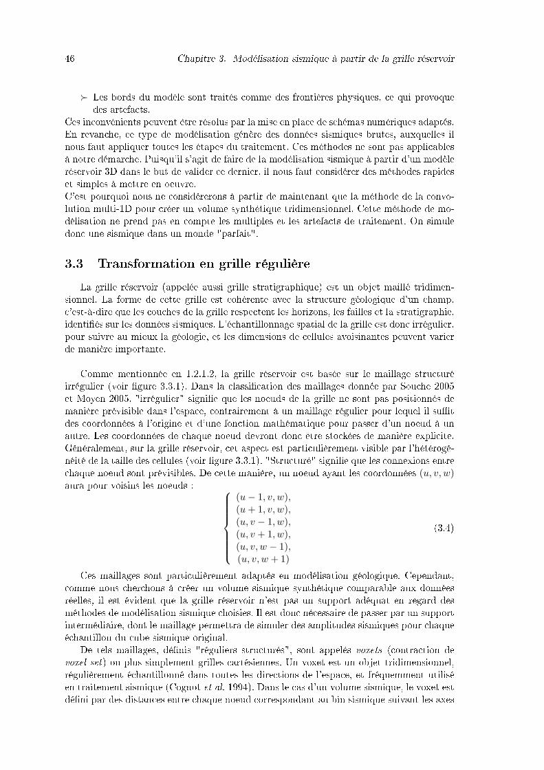
46 Chapitre 3. Modélisation sismique à partir de la grille réservoir
� Les bords du modèle sont traités comme des frontières physiques, ce qui provoquedes artefacts.
Ces inconvénients peuvent être résolus par la mise en place de schémas numériques adaptés.En revanche, ce type de modélisation génère des données sismiques brutes, auxquelles ilnous faut appliquer toutes les étapes du traitement. Ces méthodes ne sont pas applicablesà notre démarche. Puisqu'il s'agit de faire de la modélisation sismique à partir d'un modèleréservoir 3D dans le but de valider ce dernier, il nous faut considérer des méthodes rapideset simples à mettre en oeuvre.C'est pourquoi nous ne considérerons à partir de maintenant que la méthode de la convo-lution multi-1D pour créer un volume synthétique tridimensionnel. Cette méthode de mo-délisation ne prend pas en compte les multiples et les artefacts de traitement. On simuledonc une sismique dans un monde "parfait".
3.3 Transformation en grille régulièreLa grille réservoir (appelée aussi grille stratigraphique) est un objet maillé tridimen-
sionnel. La forme de cette grille est cohérente avec la structure géologique d'un champ,c'est-à-dire que les couches de la grille respectent les horizons, les failles et la stratigraphie,identi�és sur les données sismiques. L'échantillonnage spatial de la grille est donc irrégulier,pour suivre au mieux la géologie, et les dimensions de cellules avoisinantes peuvent varierde manière importante.
Comme mentionnée en 1.2.1.2, la grille réservoir est basée sur le maillage structuréirrégulier (voir �gure 3.3.1). Dans la classi�cation des maillages donnée par Souche 2005et Moyen 2005, "irrégulier" signi�e que les noeuds de la grille ne sont pas positionnés demanière prévisible dans l'espace, contrairement à un maillage régulier pour lequel il su�tdes coordonnées à l'origine et d'une fonction mathématique pour passer d'un noeud à unautre. Les coordonnées de chaque noeud devront donc être stockées de manière explicite.Généralement, sur la grille réservoir, cet aspect est particulièrement visible par l'hétérogé-néité de la taille des cellules (voir �gure 3.3.1). "Structuré" signi�e que les connexions entrechaque noeud sont prévisibles. De cette manière, un noeud ayant les coordonnées (u, v, w)aura pour voisins les noeuds :
(u− 1, v, w),(u+ 1, v, w),(u, v − 1, w),(u, v + 1, w),(u, v, w − 1),(u, v, w + 1)
(3.4)
Ces maillages sont particulièrement adaptés en modélisation géologique. Cependant,comme nous cherchons à créer un volume sismique synthétique comparable aux donnéesréelles, il est évident que la grille réservoir n'est pas un support adéquat en regard desméthodes de modélisation sismique choisies. Il est donc nécessaire de passer par un supportintermédiaire, dont le maillage permettra de simuler des amplitudes sismiques pour chaqueéchantillon du cube sismique original.
De tels maillages, dé�nis "réguliers structurés", sont appelés voxets (contraction devoxel set) ou plus simplement grilles cartésiennes. Un voxet est un objet tridimensionnel,régulièrement échantillonné dans toutes les directions de l'espace, et fréquemment utiliséen traitement sismique (Cognot et al. 1994). Dans le cas d'un volume sismique, le voxet estdé�ni par des distances entre chaque noeud correspondant au bin sismique suivant les axes

3.3. Transformation en grille régulière 47
Fig. 3.3.1 � Cellules des maillages "CPG" (irrégulier structuré) et cartésiens (régulierstructuré).
horizontaux et au pas de temps d'enregistrement dt de la sismique, suivant l'axe vertical.Les propriétés de la grille réservoir doivent être transférées dans ce nouveau support poursimuler un volume sismique synthétique. Ce transfert introduit un changement d'échelledes propriétés entre la grille réservoir et le voxet. En e�et, considérant les dimensionsusuelles d'une cellule de la grille réservoir face à celles d'une cellule du voxet, nous voyonsqu'une propriété donnée sera sous-échantillonnée suivant l'axe vertical et sur-échantillonnéesuivant les axes horizontaux. Ce dernier point ne pose pas de problème particulier. Le sur-échantillonnage latéral assure le respect de la structure de la grille. Le sous-échantillonnageen revanche, provoque la décimation de l'hétérogénéité verticale d'une propriété réservoirvers une expression discrétisée tous les dt, ce qui n'est pas une tâche triviale.Pour éviter d'avoir à gérer cela, nous utiliserons un "voxet déformé". Globalement, cevoxet déformé peut être perçu comme un ensemble de puits virtuels à chaque point duquadrillage dé�ni en x, y. Verticalement, l'échantillonnage est basé sur l'intersection dechaque pseudo-puits avec la grille réservoir, c'est-à-dire que pour chaque couche du mo-dèle, les valeurs des propriétés et l'épaisseur des couches seront respectées (voir les �gures3.3.2 et 3.3.3). Ainsi, la complexité structurale du réservoir est préservée, tout en évitant lechangement d'échelle suivant l'axe vertical. Le produit de convolution prendra en charge lechangement d'échelle verticale. Dans la suite du manuscrit, nous ferons référence au voxetdéformé sous le nom de voxet.
Fig. 3.3.2 � Transformation d'une cellule réservoir en une série de voxels (cellules du voxet).

48 Chapitre 3. Modélisation sismique à partir de la grille réservoir
Fig. 3.3.3 � L'intersection de la grille réservoir (exemple du champ Alpha) avec un pseudopuits (en rouge) permet de récupérer les propriétés du réservoir sans changement d'échelle.
3.4 Evaluation des modélisations sur le champ Alpha
La validation de la modélisation à partir d'une grille réservoir est illustrée ci-après avecles données du champ Alpha.
3.4.1 E�ets du changement de support Sismique-Réservoir-Voxet
La �gure 3.4.1 montre les résultats de l'inversion stochastique du champ Alpha, décritedans le chapitre 2, sous trois supports di�érents : la grille sismique (sur la �gure à gauche),après upscaling (moyenne arithmétique) dans la grille réservoir (au milieu) et après trans-formation dans le voxet (à droite).L'upscaling de l'échelle sismique à l'échelle réservoir provoque une perte d'information.La présence d'artefacts semble être limitée au toit et à la base du réservoir (les zonesrouges sur la �gure centrale 3.4.1. La transformation de la grille réservoir au voxet n'induitpas de perte d'information. On voit juste un e�et de pixellisation très �n.La �gure 3.4.2 montre le nombre d'échantillons sismiques moyennés par cellule du ré-servoir, et l'écart-type de ces échantillons, sous la forme d'un pourcentage de variation parrapport à la moyenne. Le fait que l'écart-type des échantillons dans le modèle réservoirreste faible, suggère que le changement d'échelle a été réalisé de manière satisfaisante.
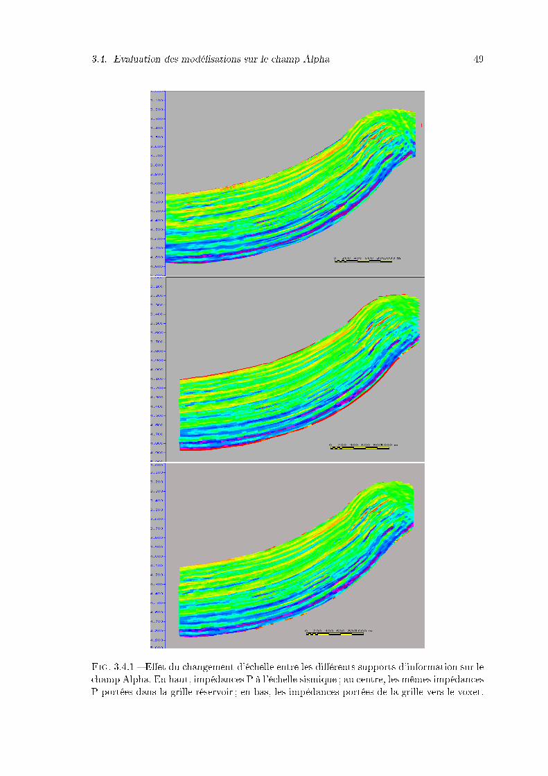
3.4. Evaluation des modélisations sur le champ Alpha 49
Fig. 3.4.1 � E�et du changement d'échelle entre les di�érents supports d'information sur lechamp Alpha. En haut, impédances P à l'échelle sismique ; au centre, les mêmes impédancesP portées dans la grille réservoir ; en bas, les impédances portées de la grille vers le voxet.
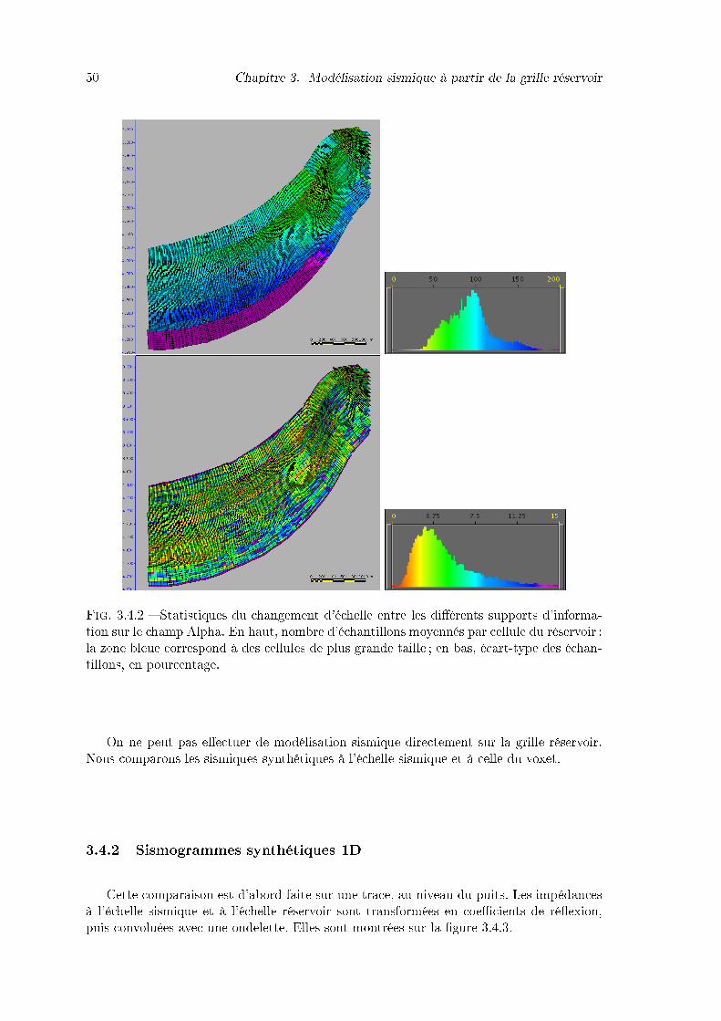
50 Chapitre 3. Modélisation sismique à partir de la grille réservoir
Fig. 3.4.2 � Statistiques du changement d'échelle entre les di�érents supports d'informa-tion sur le champ Alpha. En haut, nombre d'échantillons moyennés par cellule du réservoir ;la zone bleue correspond à des cellules de plus grande taille ; en bas, écart-type des échan-tillons, en pourcentage.
On ne peut pas e�ectuer de modélisation sismique directement sur la grille réservoir.Nous comparons les sismiques synthétiques à l'échelle sismique et à celle du voxet.
3.4.2 Sismogrammes synthétiques 1D
Cette comparaison est d'abord faite sur une trace, au niveau du puits. Les impédancesà l'échelle sismique et à l'échelle réservoir sont transformées en coe�cients de ré�exion,puis convoluées avec une ondelette. Elles sont montrées sur la �gure 3.4.3.
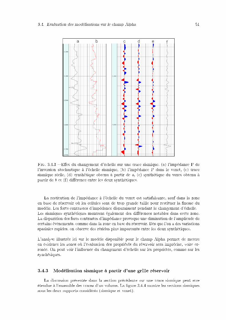
3.4. Evaluation des modélisations sur le champ Alpha 51
Fig. 3.4.3 � E�et du changement d'échelle sur une trace sismique. (a) l'impédance P del'inversion stochastique à l'échelle sismique, (b) l'impédance P dans le voxet, (c) tracesismique réelle, (d) synthétique obtenu à partir de a, (e) synthétique du voxet obtenu àpartir de b et (f) di�érence entre les deux synthétiques.
La restitution de l'impédance à l'échelle du voxet est satisfaisante, sauf dans la zoneen base de réservoir où les cellules sont de trop grande taille pour restituer la �nesse dumodèle. Les forts contrastes d'impédance disparaissent pendant le changement d'échelle.Les sismiques synthétiques montrent également des di�érences notables dans cette zone.La disparition des forts contrastes d'impédance provoque une diminution de l'amplitude decertains évènements, comme dans la zone en base du réservoir. Dès que l'on a des variationsspatiales rapides, on observe des résidus plus importants entre les deux synthétiques.L'analyse illustrée ici sur le modèle disponible pour le champ Alpha permet de mettreen évidence les zones où l'évaluation des propriétés du réservoir sera imprécise, voire er-ronée. On peut voir l'in�uence du changement d'échelle sur les propriétés, comme sur lessynthétiques.
3.4.3 Modélisation sismique à partir d'une grille réservoirLa discussion présentée dans la section précédente sur une trace sismique peut être
étendue à l'ensemble des traces d'un volume. La �gure 3.4.4 montre les sections sismiquessous les deux supports considérés (sismique et voxet).
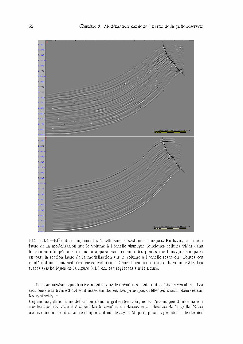
52 Chapitre 3. Modélisation sismique à partir de la grille réservoir
Fig. 3.4.4 � E�et du changement d'échelle sur les sections sismiques. En haut, la sectionissue de la modélisation sur le volume à l'échelle sismique (quelques cellules vides dansle volume d'impédance sismique apparaissent comme des points sur l'image sismique) ;en bas, la section issue de la modélisation sur le volume à l'échelle réservoir. Toutes cesmodélisations sont réalisées par convolution 1D sur chacune des traces du volume 3D. Lestraces synthétiques de la �gure 3.4.3 ont été replacées sur la �gure.
La comparaison qualitative montre que les résultats sont tout à fait acceptables. Lessections de la �gure 3.4.4 sont assez similaires. Les principaux ré�ecteurs sont observés surles synthétiques.Cependant, dans la modélisation dans la grille réservoir, nous n'avons pas d'informationsur les épontes, c'est-à-dire sur les intervalles au dessus et en dessous de la grille. Nousavons donc un contraste très important sur les synthétiques, pour le premier et le dernier
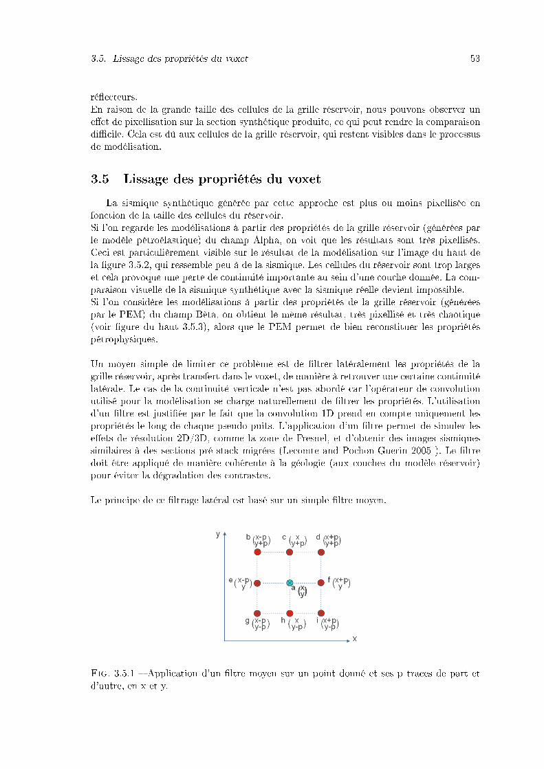
3.5. Lissage des propriétés du voxet 53
ré�ecteurs.En raison de la grande taille des cellules de la grille réservoir, nous pouvons observer une�et de pixellisation sur la section synthétique produite, ce qui peut rendre la comparaisondi�cile. Cela est dû aux cellules de la grille réservoir, qui restent visibles dans le processusde modélisation.
3.5 Lissage des propriétés du voxetLa sismique synthétique générée par cette approche est plus ou moins pixellisée en
fonction de la taille des cellules du réservoir.Si l'on regarde les modélisations à partir des propriétés de la grille réservoir (générées parle modèle pétroélastique) du champ Alpha, on voit que les résultats sont très pixellisés.Ceci est particulièrement visible sur le résultat de la modélisation sur l'image du haut dela �gure 3.5.2, qui ressemble peu à de la sismique. Les cellules du réservoir sont trop largeset cela provoque une perte de continuité importante au sein d'une couche donnée. La com-paraison visuelle de la sismique synthétique avec la sismique réelle devient impossible.Si l'on considère les modélisations à partir des propriétés de la grille réservoir (généréespar le PEM) du champ Bêta, on obtient le même résultat, très pixellisé et très chaotique(voir �gure du haut 3.5.3), alors que le PEM permet de bien reconstituer les propriétéspétrophysiques.Un moyen simple de limiter ce problème est de �ltrer latéralement les propriétés de lagrille réservoir, après transfert dans le voxet, de manière à retrouver une certaine continuitélatérale. Le cas de la continuité verticale n'est pas abordé car l'opérateur de convolutionutilisé pour la modélisation se charge naturellement de �ltrer les propriétés. L'utilisationd'un �ltre est justi�ée par le fait que la convolution 1D prend en compte uniquement lespropriétés le long de chaque pseudo-puits. L'application d'un �ltre permet de simuler lese�ets de résolution 2D/3D, comme la zone de Fresnel, et d'obtenir des images sismiquessimilaires à des sections pré stack migrées (Lecomte and Pochon-Guerin 2005 ). Le �ltredoit être appliqué de manière cohérente à la géologie (aux couches du modèle réservoir)pour éviter la dégradation des contrastes.Le principe de ce �ltrage latéral est basé sur un simple �ltre moyen.
Fig. 3.5.1 � Application d'un �ltre moyen sur un point donné et ses p traces de part etd'autre, en x et y.

54 Chapitre 3. Modélisation sismique à partir de la grille réservoir
Lors de la création du voxet, on crée une propriété qui conserve la position et l'indexdes couches de la grille réservoir. Le �ltre est ensuite appliqué couche après couche. Pourun �ltre de dimension p, en un point donné a(x, y), on calcule la moyenne des points de ptraces de part et d'autre de a, tel que illustré sur le schéma 3.5.1.En appliquant ce �ltre sur les impédances dans les grilles réservoir des champs Alphaet Bêta, on obtient l'image du bas des �gures 3.5.2 et 3.5.3, qui ont plus l'apparenced'une image sismique, et permettent de faire une comparaison de meilleure qualité avec lesdonnées réelles.
Fig. 3.5.2 � Application d'un �ltre moyen sur la section sismique issue des propriétés duPEM du champ Alpha. En haut, la section brute ; en bas, la section �ltrée.
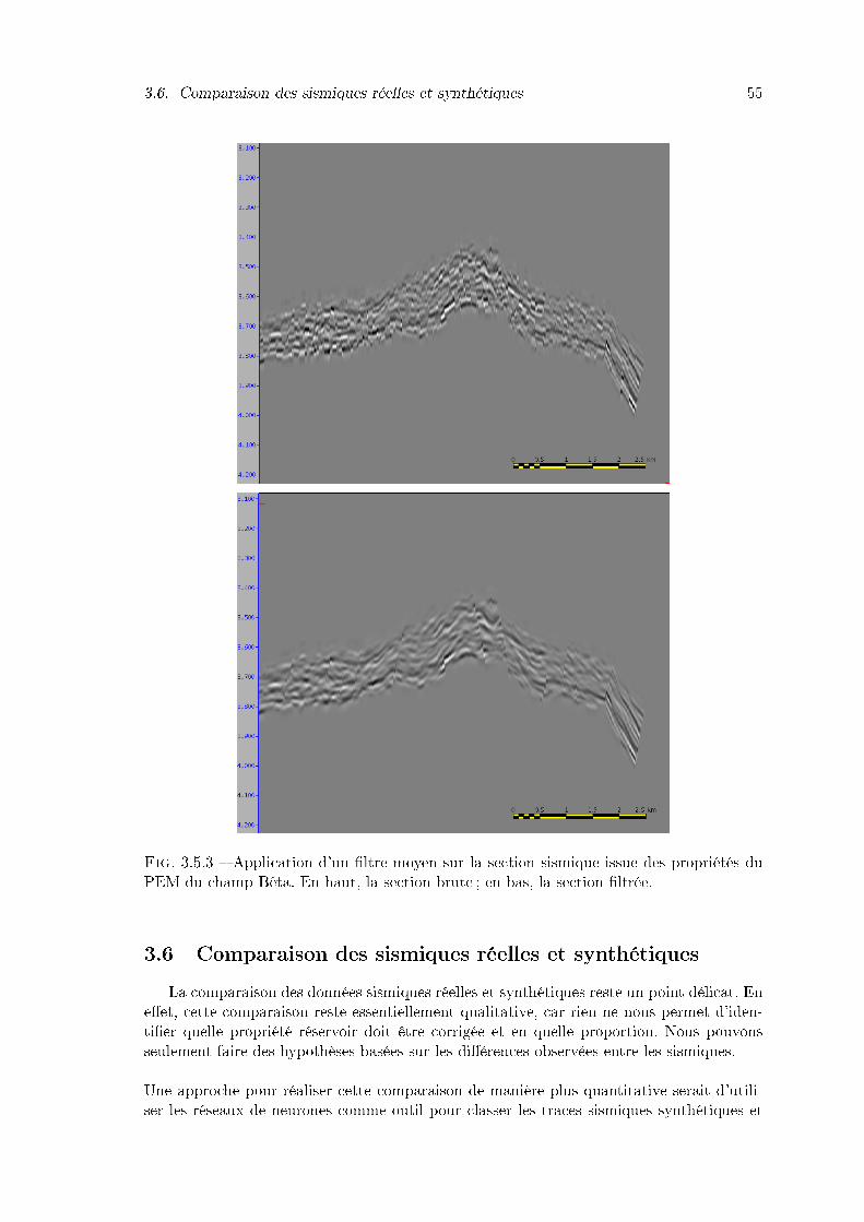
3.6. Comparaison des sismiques réelles et synthétiques 55
Fig. 3.5.3 � Application d'un �ltre moyen sur la section sismique issue des propriétés duPEM du champ Bêta. En haut, la section brute ; en bas, la section �ltrée.
3.6 Comparaison des sismiques réelles et synthétiquesLa comparaison des données sismiques réelles et synthétiques reste un point délicat. En
e�et, cette comparaison reste essentiellement qualitative, car rien ne nous permet d'iden-ti�er quelle propriété réservoir doit être corrigée et en quelle proportion. Nous pouvonsseulement faire des hypothèses basées sur les di�érences observées entre les sismiques.Une approche pour réaliser cette comparaison de manière plus quantitative serait d'utili-ser les réseaux de neurones comme outil pour classer les traces sismiques synthétiques et
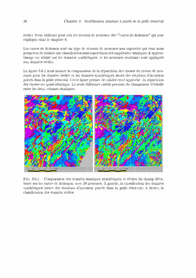
56 Chapitre 3. Modélisation sismique à partir de la grille réservoir
réelles. Nous utilisons pour cela les réseaux de neurones dits "cartes de Kohonen" qui sontexpliqués dans le chapitre 6.Les cartes de Kohonen sont un type de réseaux de neurones non supervisé qui vont nouspermettre de réaliser une classi�cation sans supervision des amplitudes sismiques. L'appren-tissage est réalisé sur les données synthétiques, et les neurones résultants sont appliquésaux données réelles.La �gure 3.6.1 nous montre la comparaison de la répartition des classes du réseau de neu-rones pour les données réelles et les données synthétiques issues des résultats d'inversionportés dans la grille réservoir. Cette �gure permet de valider cette approche : la répartitiondes classes est quasi-identique. La seule di�érence visible provient du changement d'échelleentre les deux volumes sismiques.
Fig. 3.6.1 � Comparaison des données sismiques synthétiques et réelles du champ Bêta,basée sur les cartes de Kohonen, avec 20 neurones. A gauche, la classi�cation des donnéessynthétiques issues des résultats d'inversion portés dans la grille réservoir ; à droite, laclassi�cation des données réelles.

3.6. Comparaison des sismiques réelles et synthétiques 57
La �gure 3.6.2 montre l'application de cette approche sur les données synthétiquesissues des propriétés pétrophysiques obtenues avec le PEM : l'image du bas montre leszones où un neurone se trouve au même endroit sur les sismiques réelles et synthétiques,donc les zones où les traces synthétiques sont bien corrélées avec les traces sismiques.La couleur foncée montre la concordance des classes entre les deux volumes de données.L'image étant principalement claire, on voit que les données synthétiques générées par lePEM ne correspondent pas aux données réelles. Dans ces zones, les propriétés du réservoirdoivent donc être modi�ées.Cette approche permet de véri�er si la sismique synthétique est proche des données réellesou pas, sur une carte 2D qui identi�e les zones cohérentes. La seule di�culté est de trouverun moyen de tirer avantage de ces cartes.
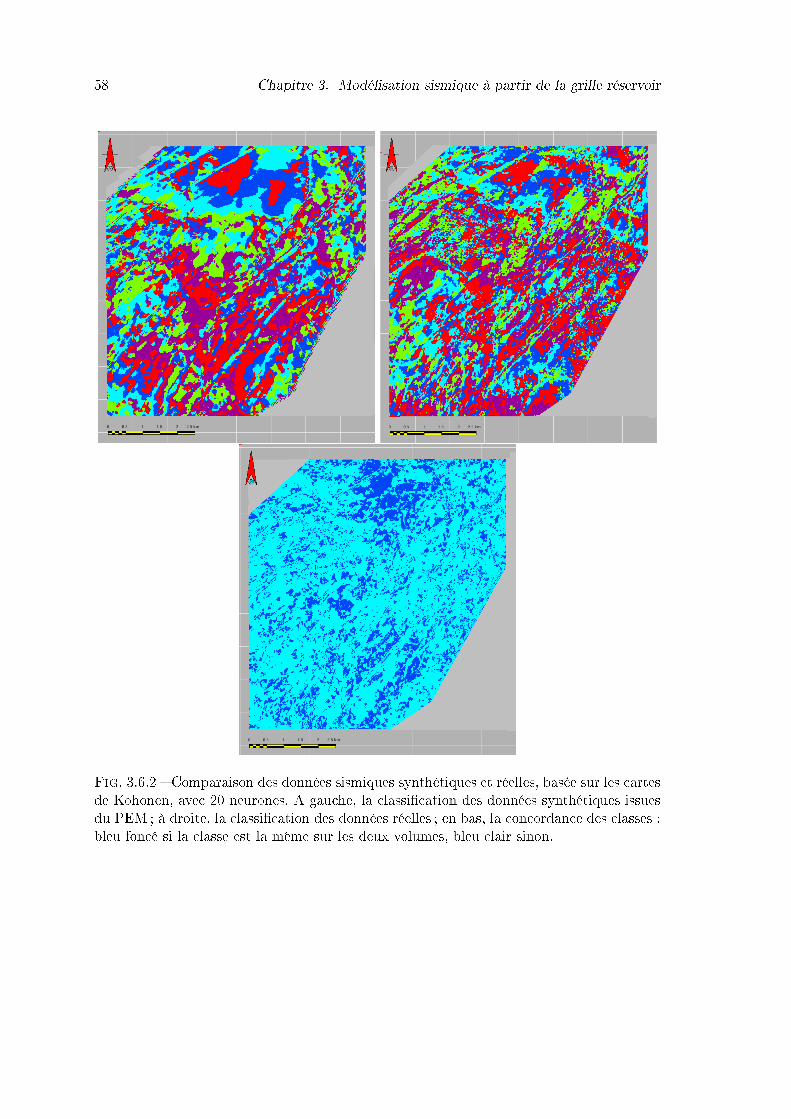
58 Chapitre 3. Modélisation sismique à partir de la grille réservoir
Fig. 3.6.2 � Comparaison des données sismiques synthétiques et réelles, basée sur les cartesde Kohonen, avec 20 neurones. A gauche, la classi�cation des données synthétiques issuesdu PEM ; à droite, la classi�cation des données réelles ; en bas, la concordance des classes :bleu foncé si la classe est la même sur les deux volumes, bleu clair sinon.
3.7. Conclusions et perspectives 59
3.7 Conclusions et perspectivesToutes les sismiques synthétiques calculées dans cette thèse sont réalisées avec un mo-
dèle convolutionnel 1D appliqué à chacune des traces sismiques du volume 3D de propriétésconsidérées.La taille des cellules du modèle réservoir est un compromis entre temps de calcul pour lessimulateurs de �uides et dimensions des hétérogénéités à intégrer dans le modèle. Les pertesd'informations liées au changement d'échelle, lors du passage de la sismique au réservoir,peuvent être analysées à partir de statistiques sur les échantillons portés dans les cellulesdu réservoir. Ceci permet d'avoir un regard critique sur la pertinence de la grille disponiblepour la caractérisation du réservoir considéré. Quand il s'agit de retrouver le remplissagede la grille réservoir à partir des données sismiques, cette évaluation n'est possible qu'encomparant les données sismiques synthétiques et réelles, ce qui n'est pas une tâche triviale.L'utilisation des réseaux de neurones de type Kohonen pour faire cette comparaison estune approche intéressante car semi-automatique, mais qui n'exprime la di�érence des tracesque sur une carte 2D.En général, la réponse sismique de propriétés pétrophysiques n'est testée qu'au niveaudes puits. Cette approche de modélisation sismique sur grille réservoir permet d'e�ectuerce test sur l'ensemble du volume sismique, et rend possible la comparaison avec les donnéesréelles. La modélisation sismique à partir d'une grille réservoir est donc une étape essen-tielle pour la validation de scénarii pétrophysiques et du remplissage en regard des donnéessismiques. Le plus grand béné�ce de cette approche réside dans la possibilité de visualiserla qualité de scénarii structuraux et de remplissage.

60 Chapitre 3. Modélisation sismique à partir de la grille réservoir
Chapitre 4
L'impact des incertitudes structurales
Les études en caractérisation réservoir utilisent les données disponibles pour construireun modèle réservoir et déterminer les propriétés qui le caractérisent. Le modèle utilisécorrespond à la vision la plus probable du réservoir, alors qu'il est possible de construireplusieurs modèles réservoirs à partir des mêmes données. La gestion des incertitudes ap-paraît à chaque étape de la vie du réservoir. En caractérisation réservoir, ces incertitudesenglobent les paramètres géométriques (taille du réservoir, emplacement des horizons, desfailles, etc.) et les paramètres pétrophysiques (perméabilité, porosités, etc.). Mais le plussouvent, les incertitudes que l'on regarde en caractérisation réservoir ne correspondentqu'aux incertitudes sur les propriétés.Nous cherchons à remplir la grille réservoir de propriétés pétrophysiques dans le but desimuler son comportement pendant sa production. Mais sans la prise en compte des incer-titudes liées aux paramètres géométriques, ou incertitudes structurales, nous ignorons siles résultats des diverses études sont correctement positionnés dans l'espace.Les incertitudes structurales sont les sources d'erreurs les plus di�ciles à évaluer lors de laconstruction de la grille réservoir. Pour illustrer l'e�et de ces incertitudes, nous décrivonsici la cas de la grille réservoir du champ Alpha, qui montre un décalage entre les horizonspointés sur la sismique et les horizons correspondant de la grille réservoir. Un simple re-port en temps ne su�t pas à corriger ces di�érences. Dans le cas présent, les di�érencesobservées sont dues à une confusion dans le modèle de vitesse à utiliser. Il résulte de cesdi�érences que l'interprétation géologique portée dans la grille montre un chenal près de20ms au dessus de sa position réelle.Dans le cas du champ Alpha, l'interprétation géologique était déjà connue, ce qui a per-mis d'identi�er le problème rapidement. Mais que se passe-t-il lorsque l'on commence lestravaux de caractérisation réservoir, et que l'interprétation n'est pas encore �nalisée ? Com-ment ces incertitudes vont-elles a�ecter notre vision du réservoir ?Les incertitudes structurales doivent être prises en compte dans toutes études de caracté-risation réservoir. Elles doivent au moins être évaluées avant de choisir un unique modèlede réservoir. Pour montrer l'e�et que peuvent avoir ces incertitudes sur le remplissage duréservoir, nous proposons d'utiliser le champ Alpha pour réaliser une étude de la répartitiondes faciès dans la grille réservoir par classi�cation des attributs sismiques, à laquelle nousajoutons une étape de réalisation stochastique de la géométrie du modèle réservoir.
61

62 Chapitre 4. L'impact des incertitudes structurales
4.1 IntroductionReservoir characterization studies use all available data to build a reservoir model and
determine its properties. The model used is the more probable vision of the reservoir, eventhough it is possible to build several reservoirs models from these data. Uncertainty ma-nagement appears at each stage of the life of the reservoir. In reservoir characterization,these uncertainties include geometric parameters (size of reservoir, location of horizons,faults, etc.) and petrophysical parameters (permeability, porosity, etc.). But in most cases,the uncertainties that we use in reservoir characterization re�ect only the petrophysicalproperties.We want to in�ll the reservoir grid with petrophysical properties in order to simulate itsdynamic behaviour during the production. But if we do not take into account the uncer-tainties associated to geometric parameters (or structural uncertainties), we do not knowif the results of various studies are properly positioned in space.One question we need to ask is : How will these uncertainties a�ect our view of the reser-voir ?In the case of the Alpha �eld presented hereafter, the geological interpretation is alreadyknown. We therefore propose to use the Alpha �eld to study the impact of uncertainties onthe structural interpretation of the reservoir (Neau et al. 2007). The di�erences of positionobserved on this dataset will be used to calibrate the uncertainties for this process.In the example of Alpha �elds, the uncertainties are related to the velocity model for thetime/depth conversion. Other types of uncertainty can lead to misinterpretation (Thoreet al. 2002). The most important ones, in addition to uncertainties related to the time/depthconversion, are as follows :
� Uncertainties related to seismic picking :The character of a seismic re�ector can vary laterally, induced by changes in staticor dynamic properties, by variations in facies or types of �uids, or by the presenceof multiples.
� Uncertainties related to fault zones :A re�ector can be degraded by the presence of a shadow zone, or may be lost in agrinding zone.
All these uncertainties are the most di�cult sources of errors to assess during theconstruction of the reservoir grid. To take into account these uncertainties, we propose atypical study of facies repartition in the reservoir grid by classi�cation of seismic attributes,to which we add a step of stochastic simulation of reservoir models (see work�ow 4.1.1).
4.2 Multiple reservoir grid realizationsBuilding a reservoir grid must go through an interpretation phase of all available data.
The elementary framework of a reservoir model consists in a set of horizons, faults andwell markers. Horizons and faults are interpreted on the seismic data, and both are clo-sely related. Thus, the generation of multiple models should be done by maintaining therelationships horizons/faults/markers. Each one of these objects brings its own uncertain-ties that we need to quantify before integrating them in the simulation of multiple models.Thore et al. 2002 makes a complete review of the uncertainties having an e�ect on reservoirmodels, and explains how to quantify them. Once known, those uncertainties, symbolizedby 3D vectors, are applied at each horizon (and fault) node. With these vectors and thebase case interpretation, we want to create several models, that is to say, to generate
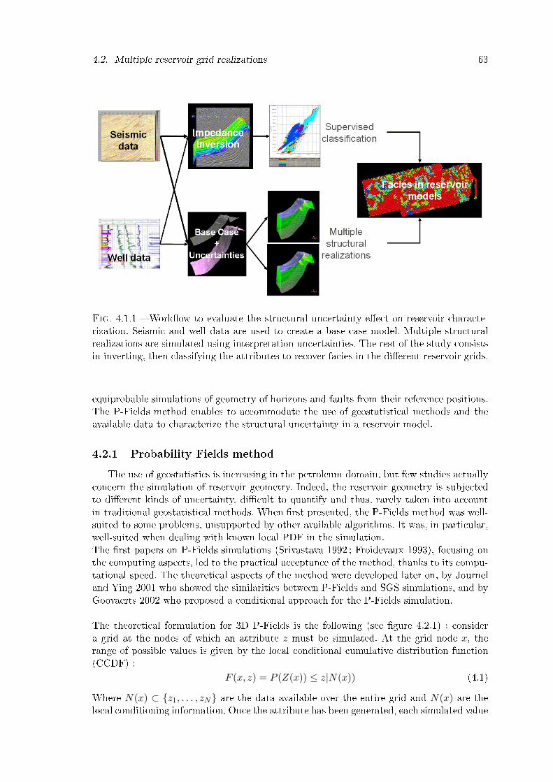
4.2. Multiple reservoir grid realizations 63
Fig. 4.1.1 � Work�ow to evaluate the structural uncertainty e�ect on reservoir characte-rization. Seismic and well data are used to create a base case model. Multiple structuralrealizations are simulated using interpretation uncertainties. The rest of the study consistsin inverting, then classifying the attributes to recover facies in the di�erent reservoir grids.
equiprobable simulations of geometry of horizons and faults from their reference positions.The P-Fields method enables to accommodate the use of geostatistical methods and theavailable data to characterize the structural uncertainty in a reservoir model.
4.2.1 Probability Fields methodThe use of geostatistics is increasing in the petroleum domain, but few studies actually
concern the simulation of reservoir geometry. Indeed, the reservoir geometry is subjectedto di�erent kinds of uncertainty, di�cult to quantify and thus, rarely taken into accountin traditional geostatistical methods. When �rst presented, the P-Fields method was well-suited to some problems, unsupported by other available algorithms. It was, in particular,well-suited when dealing with known local PDF in the simulation.The �rst papers on P-Fields simulations (Srivastava 1992 ; Froidevaux 1993), focusing onthe computing aspects, led to the practical acceptance of the method, thanks to its compu-tational speed. The theoretical aspects of the method were developed later on, by Journeland Ying 2001 who showed the similarities between P-Fields and SGS simulations, and byGoovaerts 2002 who proposed a conditional approach for the P-Fields simulation.The theoretical formulation for 3D P-Fields is the following (see �gure 4.2.1) : considera grid at the nodes of which an attribute z must be simulated. At the grid node x, therange of possible values is given by the local conditional cumulative distribution function(CCDF) :
F (x, z) = P (Z(x)) ≤ z|N(x)) (4.1)Where N(x) ⊂ {z1, . . . , zN} are the data available over the entire grid and N(x) are thelocal conditioning information. Once the attribute has been generated, each simulated value

64 Chapitre 4. L'impact des incertitudes structurales
zsim at the location x may be obtained by computing the inverse of the local CCDF :
zsim(x) = F−1 [x; p(x)] (4.2)
The values of p are considered as a realization of a uniform random function P (x), simu-lated with a given variogram.The 3D P-Fields simulation proceeds as following :
1. Generate a set of grids with spatially correlated values, uniformly distributed between0 and 1.
2. Backtransform the obtained values into the expected distribution. This results in arelative displacement, proportional to the length of the uncertainty vector.
Then, we apply the relative displacement obtained at each node on the reference horizon.
Fig. 4.2.1 � Operating principle for the P-Fields simulation, applied on a surface. Anuncertainty value zsim(u) is added up to the initial surface at each node u. This value isdrawn in the local CDF. From Thore et al. 2002.
4.2.2 Uncertainty representationStructural uncertainties are represented as 3D vectors at each horizon (or fault) nodes.
These vectors give the maximum absolute value of uncertainty to be applied at one givenpoint. Each vector is applied symmetrically on both sides of the reference nodes and theyshow the possible interval of simulated positions for the new horizons (see red lines on�gure 4.2.2).
Since we want to generate new horizons consistent with the geology, we also need toassociate a correlation length to control the lateral continuity of the new horizons. Inpractice, with a small correlation length, we allow the simulations to introduce small scaledisturbances and the resulting horizons are very discontinuous. On the other hand, if thiscorrelation length is long, the horizons are continuous (see �gure 4.2.2).

4.2. Multiple reservoir grid realizations 65
Fig. 4.2.2 � In�uence of the correlation length on the simulated horizons. The dotted redlines represent the uncertainty interval, the black line the reference horizon. The blue andgreen lines are the simulated horizons respectively for a small and a long correlation length.The simulation is constrained by two wells.
Note on well integration At the well location, the exact depth of a marker is known,and the uncertainty at this point is null. Around the well location, the nearby points (atone correlation length away) are sensitive to the constraining points and should have lesseruncertainties. This introduces a bias in the original structural uncertainties of these points.
Note on model coherency As cited previously, the generation of new surfaces shouldbe done by maintaining the relationships between horizons and faults. A correlation factorbetween horizons is introduced in the process. It de�nes how structural uncertainties fromthe reservoir top will a�ect the other horizons of the model. Indeed, when a simulationis done on the reservoir top, the transformations are transmitted to the other surfacesdepending on this correlation factor. Then, small perturbations are applied individuallyon each horizon, so that these perturbations, added up to the uncertainties from the tophorizon, are within the local uncertainty range. For example, a correlation factor of 80%means that the uncertainty applied on a horizon results from 64% of deformations on thereservoir top and from 36% of local perturbations.
4.2.3 Application on Alpha �eld
The geological overview and the description of available data for the Alpha �eld can beseen in Chapter 2. The reservoir model from Alpha �eld consists in six reference horizonsidenti�ed on seismic data and four fault surfaces. As shown on �gure 4.2.3, errors onvelocity models induced a gap between the reference horizons and the corresponding layersin the reservoir grid. The di�erences are computed, and shown on �gure 4.2.4 with theirhistograms.
In real cases, we can not evaluate directly the amount of structural uncertainties wehave to apply. Here, since we already know them from the misplacement between horizonsand grid layers, those di�erences will be used to de�ne the uncertainties to apply on ourreference horizons. To do so, the arithmetic mean di�erence is computed with the mapsshown in 4.2.4 for each horizon, and multiplied by 1, 5 to give some variability. We obtainthe following uncertainty values :
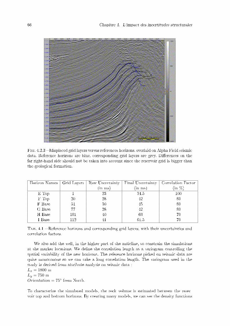
66 Chapitre 4. L'impact des incertitudes structurales
Fig. 4.2.3 � Misplaced grid layers versus references horizons, overlaid on Alpha Field seismicdata. Reference horizons are blue, corresponding grid layers are grey. Di�erences on thefar right-hand side should not be taken into account since the reservoir grid is bigger thanthe geological formation.
Horizon Names Grid Layers Raw Uncertainty Final Uncertainty Correlation Factor(in ms) (in ms) (in %)
E Top 1 23 34,5 100F Top 20 28 42 80F Base 51 30 45 80G Base 77 28 42 80H Base 101 40 60 70I Base 112 41 61,5 70
Tab. 4.1 � Reference horizons and corresponding grid layers, with their uncertainties andcorrelation factors.
We also add the well, in the higher part of the anticline, to constrain the simulationsat the marker locations. We de�ne the correlation length as a variogram controlling thespatial variability of the new horizons. The reference horizons picked on seismic data arequite monotonous so we can take a long correlation length. The variogram used in thestudy is derived from attribute analysis on seismic data :Lx = 1800 mLy = 750 mOrientation = 75◦ from North.To characterize the simulated models, the rock volume is estimated between the reser-voir top and bottom horizons. By creating many models, we can see the density functions

4.2. Multiple reservoir grid realizations 67
Fig. 4.2.4 � Computed di�erence maps between reference horizons and corresponding gridlayers, with their respective histograms. Di�erences on the far right-hand side should notbe taken into account since the reservoir grid is bigger than the geological formation.
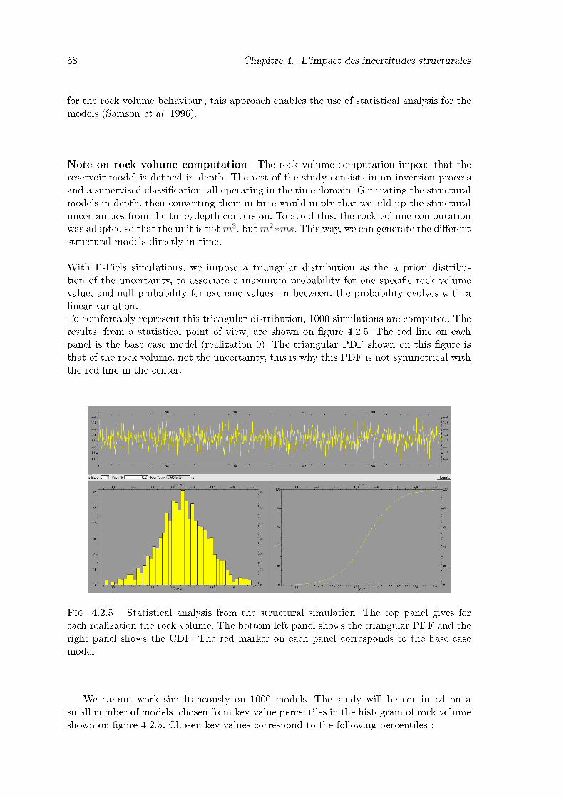
68 Chapitre 4. L'impact des incertitudes structurales
for the rock volume behaviour ; this approach enables the use of statistical analysis for themodels (Samson et al. 1996).
Note on rock volume computation The rock volume computation impose that thereservoir model is de�ned in depth. The rest of the study consists in an inversion processand a supervised classi�cation, all operating in the time domain. Generating the structuralmodels in depth, then converting them in time would imply that we add up the structuraluncertainties from the time/depth conversion. To avoid this, the rock volume computationwas adapted so that the unit is notm3, butm2∗ms. This way, we can generate the di�erentstructural models directly in time.With P-Fiels simulations, we impose a triangular distribution as the a priori distribu-tion of the uncertainty, to associate a maximum probability for one speci�c rock volumevalue, and null probability for extreme values. In between, the probability evolves with alinear variation.To comfortably represent this triangular distribution, 1000 simulations are computed. Theresults, from a statistical point of view, are shown on �gure 4.2.5. The red line on eachpanel is the base case model (realization 0). The triangular PDF shown on this �gure isthat of the rock volume, not the uncertainty, this is why this PDF is not symmetrical withthe red line in the center.
Fig. 4.2.5 � Statistical analysis from the structural simulation. The top panel gives foreach realization the rock volume. The bottom left panel shows the triangular PDF and theright panel shows the CDF. The red marker on each panel corresponds to the base casemodel.
We cannot work simultaneously on 1000 models. The study will be continued on asmall number of models, chosen from key-value percentiles in the histogram of rock volumeshown on �gure 4.2.5. Chosen key-values correspond to the following percentiles :
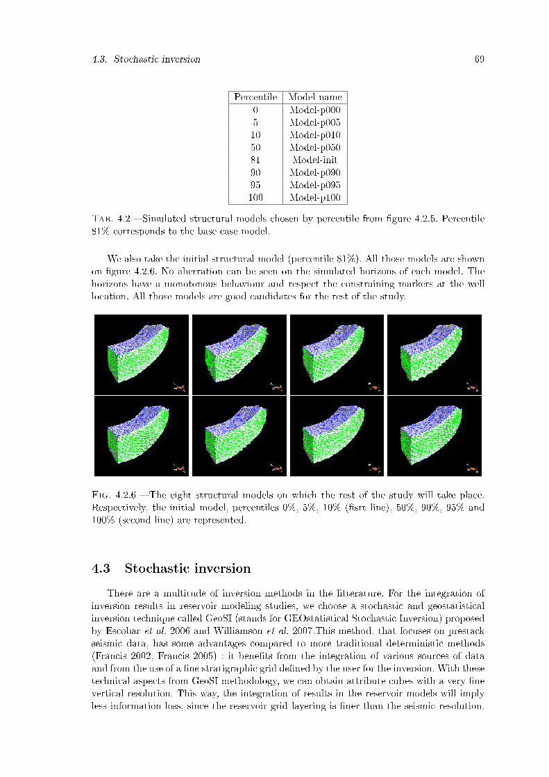
4.3. Stochastic inversion 69
Percentile Model name0 Model-p0005 Model-p00510 Model-p01050 Model-p05081 Model-init90 Model-p09095 Model-p095100 Model-p100
Tab. 4.2 � Simulated structural models chosen by percentile from �gure 4.2.5. Percentile81% corresponds to the base case model.
We also take the initial structural model (percentile 81%). All those models are shownon �gure 4.2.6. No aberration can be seen on the simulated horizons of each model. Thehorizons have a monotonous behaviour and respect the constraining markers at the welllocation. All those models are good candidates for the rest of the study.
Fig. 4.2.6 � The eight structural models on which the rest of the study will take place.Respectively, the initial model, percentiles 0%, 5%, 10% (�srt line), 50%, 90%, 95% and100% (second line) are represented.
4.3 Stochastic inversionThere are a multitude of inversion methods in the litterature. For the integration of
inversion results in reservoir modeling studies, we choose a stochastic and geostatisticalinversion technique called GeoSI (stands for GEOstatistical Stochastic Inversion) proposedby Escobar et al. 2006 and Williamson et al. 2007.This method, that focuses on prestackseismic data, has some advantages compared to more traditional deterministic methods(Francis 2002, Francis 2005) : it bene�ts from the integration of various sources of dataand from the use of a �ne stratigraphic grid de�ned by the user for the inversion. With thesetechnical aspects from GeoSI methodology, we can obtain attribute cubes with a very �nevertical resolution. This way, the integration of results in the reservoir models will implyless information loss, since the reservoir grid layering is �ner than the seismic resolution.

70 Chapitre 4. L'impact des incertitudes structurales
Moreover, this technique gives multiple equiprobable attribute realizations, re�ecting thenon unicity of the solution.
4.3.1 GeoSI operating principlesAs for Buland and Omre 2003, a Bayesian framework is proposed to compute the
probability of an impedance model m, knowing the seismic data s and the wells wl :P (m|s, wl) ∝ P (s|m).P (wl|m).P (m) (4.3)
with P (s|m) the seismic likehood, P (wl|m) the well data likehood and P (m) the priormodel. Each member of the equation 4.3 is considered as a Gaussian PDF which mean isthe squared di�erence between actual and modeled data. The most important element inthe equation is the seismic likehood, written by :
P (s|m) ∝ exp
[−1
2
∑θ
∑i
(si,θ −Gi,θ.mi)TC−1si,θ
(si,θ −Gi,θ.mi)
](4.4)
avec si,θ the seismic trace i at angle θGi,θ the synthetic seismic traceCsi,θ
the noise covariance matrix.The Gaussian posterior PDF P (m|s) is constructed by combining the Gaussian prior PDFP (m) and equation 4.4. Escobar et al. 2006 have developed an SGS-type algorithm tosample the posterior PDF : it performs a trace-by-trace decomposition of the global PDFinto a number of approximate local PDFs, which are conditioned by previously visitedtraces. Multiple realizations can therefore be e�ciently generated by sampling these localGaussian PDFs.Seismic modeling for the acoustic case is performed with a convolutional model :
s(t) = w(t) ∗ r(t) = Gθm (4.5)with w the seismic wavelet and r the re�ectivity series in time, sampled irregularly becauseof the grid layout. The re�ectivity for a given interface is based on impedance contrasts :
r =∆z2z
≈ ∆ln(z)2
valid for small re�ectivity variations (4.6)Seismic modeling for the elastic case is performed by computing the angle-variant re-
�ectivity with Fatti approximation of Zoeppritz equations :rθ ≈
12cos2θ
∆ln(Ip)− 4Is
Ipsin2θ∆ln(Is) (4.7)
4.3.2 Prior model buildingThe prior model is built in a stratigraphic grid (the inversion support) and its in�lling
based on available information (kriging of well logs, depth trends or blocky model, etc . . . ).The frame of this stratigraphic grid, de�ned in time, is built with several reference horizons,delimiting macro layers, in which a �ner layering is de�ned. Laterally, the grid is based onthe seismic bin. We create a stratigraphic model bigger than all structural models, and themicrolayering is de�ned with layers 1ms thick.
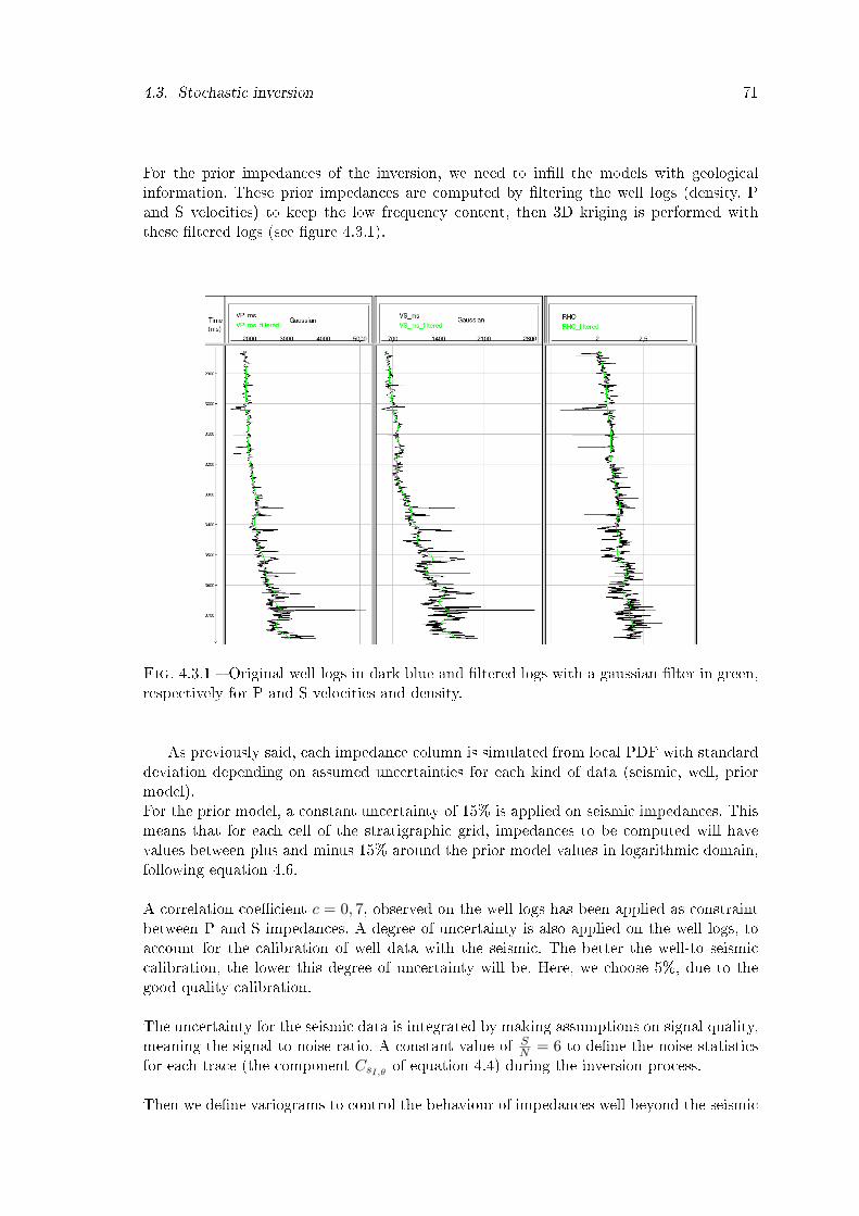
4.3. Stochastic inversion 71
For the prior impedances of the inversion, we need to in�ll the models with geologicalinformation. These prior impedances are computed by �ltering the well logs (density, Pand S velocities) to keep the low frequency content, then 3D kriging is performed withthese �ltered logs (see �gure 4.3.1).
Fig. 4.3.1 � Original well logs in dark blue and �ltered logs with a gaussian �lter in green,respectively for P and S velocities and density.
As previously said, each impedance column is simulated from local PDF with standarddeviation depending on assumed uncertainties for each kind of data (seismic, well, priormodel).For the prior model, a constant uncertainty of 15% is applied on seismic impedances. Thismeans that for each cell of the stratigraphic grid, impedances to be computed will havevalues between plus and minus 15% around the prior model values in logarithmic domain,following equation 4.6.A correlation coe�cient c = 0, 7, observed on the well logs has been applied as constraintbetween P and S impedances. A degree of uncertainty is also applied on the well logs, toaccount for the calibration of well data with the seismic. The better the well-to seismiccalibration, the lower this degree of uncertainty will be. Here, we choose 5%, due to thegood quality calibration.The uncertainty for the seismic data is integrated by making assumptions on signal quality,meaning the signal to noise ratio. A constant value of S
N = 6 to de�ne the noise statisticsfor each trace (the component CsI,θ
of equation 4.4) during the inversion process.Then we de�ne variograms to control the behaviour of impedances well beyond the seismic

72 Chapitre 4. L'impact des incertitudes structurales
resolution. The vertical component of these variograms is de�ned by the statistical analysisof well logs. We obtain a range of 18 ms, meaning 18 layers from the stratigraphic grids.The lateral component is determined from an exponential variogram with a range of 1000m, computed from seismic time-slice analysis.
4.3.3 Generation and QC of seismic attributesGeoSI being a stochastic algorithm, we have to de�ne how many realizations we want.
This number should be high enough to infer reliable statistics (mean and posterior uncer-tainty). We choose to derive 100 realizations for each attributes (P and S impedances) andthe mean is computed on the whole set of realizations. At the end of the process, we keepthe means and posterior uncertainties for each attributes and 3 individual realizations.
Fig. 4.3.2 � Inversion results at well location for P (left) and S (right) impedances. Darkblue curves are the original P and S impedances.
The �rst criterion for quality control of GeoSI inversion is to verify the coherency bet-ween actual and simulated impedances at well locations. Figure 4.3.2 shows the P andS mean impedances from the inversion process versus actual impedances from well logs.Here the correlation between inverted and actual logs is very good, with the inverted Pimpedances having a slightly higher variance than the actual P impedance log.The second criterion is the synthetic seismic obtained from inverted impedances and theirrespective residuals with the actual seismic data. Figure 4.3.3 shows an example of thison the initial model, with the actual and synthetic seismic volumes and the residuals. Wesee that the inverted impedances are in good agreement with the actual data, with overallRMS error of 4%.The �gure 4.3.4 shows an independent realization and the mean from all realizations.
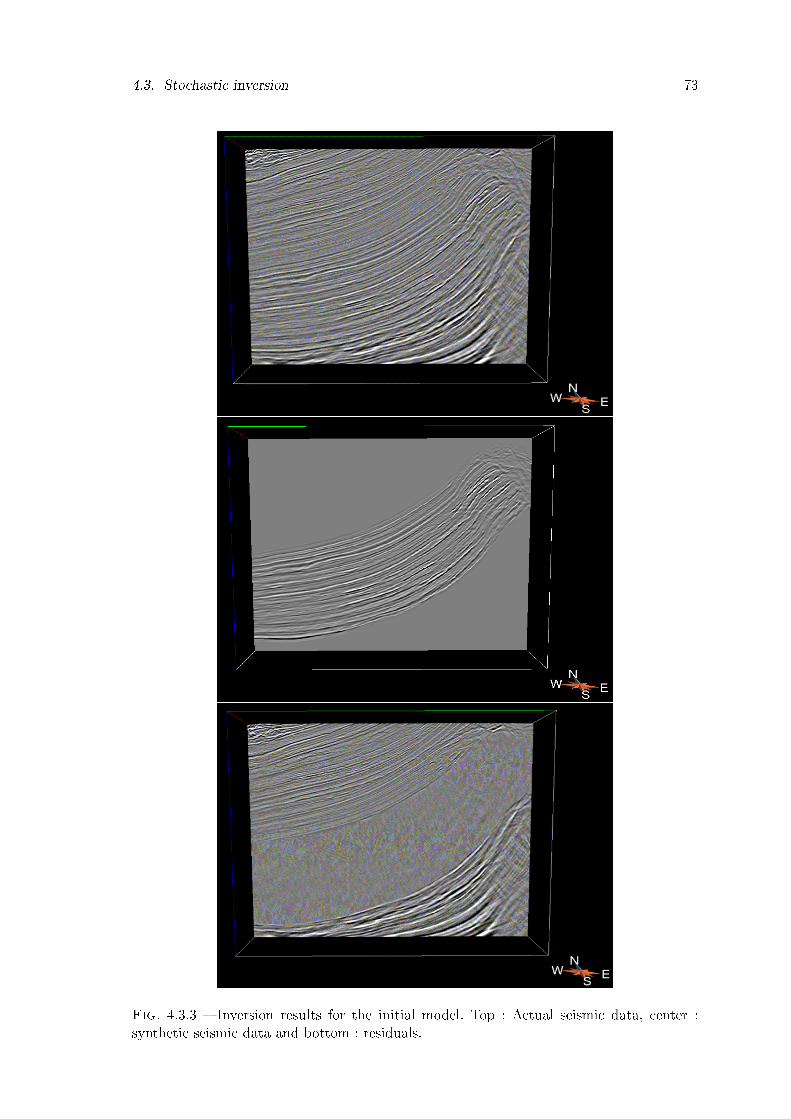
4.3. Stochastic inversion 73
Fig. 4.3.3 � Inversion results for the initial model. Top : Actual seismic data, center :synthetic seismic data and bottom : residuals.
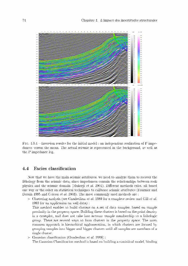
74 Chapitre 4. L'impact des incertitudes structurales
Fig. 4.3.4 � Inversion results for the initial model : an independent realization of P impe-dances versus the mean. The actual seismic is represented in the background, as well asthe P impedance log.
4.4 Facies classi�cationNow that we have the main seismic attributes, we need to analyze them to recover the
lithology from the seismic data, since impedances contain the relationships between rockphysics and the seismic domain (Mukerji et al. 2001). Di�erent methods exist, all basedone way or the other on statistical techniques to calibrate seismic attributes (Fournier andDerain 1995 and Coleou et al. 2003). The most commonly used methods are :
� Clustering analysis (see Gnadesikan et al. 1989 for a complete review and Gill et al.1993 for an application on well data) :This method enables to build clusters on a set of data samples, based on sampleproximity in the property space. Building these clusters is based on the point densityin a crossplot, and does not take into account sample membership to a lithologicgroup. There are several ways to form clusters in the property space. The mostcommon approach is hierarchical agglomeration, in which clusters are formed bygrouping samples into bigger and bigger clusters until all samples are members of asingle cluster.
� Gaussian classi�cation (Gnadesikan et al. 1989) :The Gaussian Classi�cation method is based on building a statistical model, binding
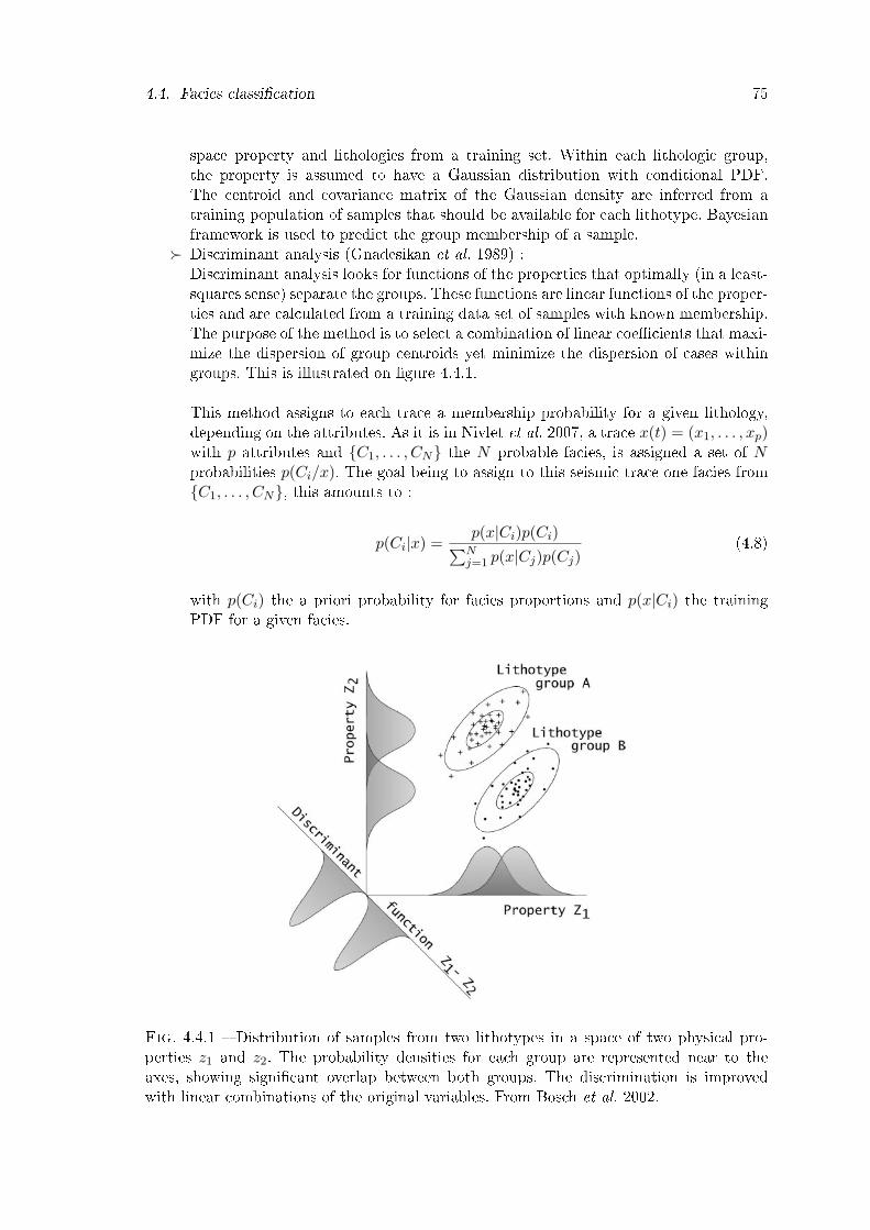
4.4. Facies classi�cation 75
space property and lithologies from a training set. Within each lithologic group,the property is assumed to have a Gaussian distribution with conditional PDF.The centroid and covariance matrix of the Gaussian density are inferred from atraining population of samples that should be available for each lithotype. Bayesianframework is used to predict the group membership of a sample.
� Discriminant analysis (Gnadesikan et al. 1989) :Discriminant analysis looks for functions of the properties that optimally (in a least-squares sense) separate the groups. These functions are linear functions of the proper-ties and are calculated from a training data set of samples with known membership.The purpose of the method is to select a combination of linear coe�cients that maxi-mize the dispersion of group centroids yet minimize the dispersion of cases withingroups. This is illustrated on �gure 4.4.1.This method assigns to each trace a membership probability for a given lithology,depending on the attributes. As it is in Nivlet et al. 2007, a trace x(t) = (x1, . . . , xp)with p attributes and {C1, . . . , CN} the N probable facies, is assigned a set of Nprobabilities p(Ci/x). The goal being to assign to this seismic trace one facies from{C1, . . . , CN}, this amounts to :
p(Ci|x) =p(x|Ci)p(Ci)∑N
j=1 p(x|Cj)p(Cj)(4.8)
with p(Ci) the a priori probability for facies proportions and p(x|Ci) the trainingPDF for a given facies.
Fig. 4.4.1 � Distribution of samples from two lithotypes in a space of two physical pro-perties z1 and z2. The probability densities for each group are represented near to theaxes, showing signi�cant overlap between both groups. The discrimination is improvedwith linear combinations of the original variables. From Bosch et al. 2002.
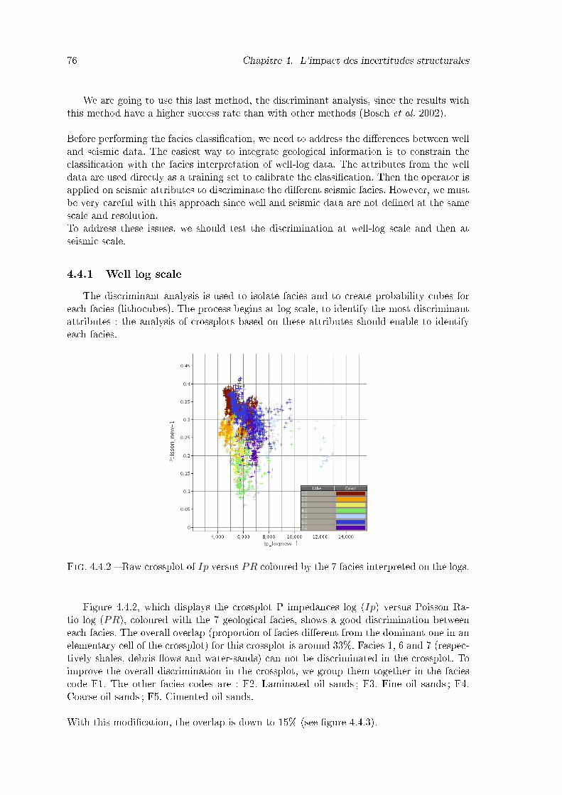
76 Chapitre 4. L'impact des incertitudes structurales
We are going to use this last method, the discriminant analysis, since the results withthis method have a higher success rate than with other methods (Bosch et al. 2002).Before performing the facies classi�cation, we need to address the di�erences between welland seismic data. The easiest way to integrate geological information is to constrain theclassi�cation with the facies interpretation of well-log data. The attributes from the welldata are used directly as a training set to calibrate the classi�cation. Then the operator isapplied on seismic attributes to discriminate the di�erent seismic facies. However, we mustbe very careful with this approach since well and seismic data are not de�ned at the samescale and resolution.To address these issues, we should test the discrimination at well-log scale and then atseismic scale.
4.4.1 Well log scaleThe discriminant analysis is used to isolate facies and to create probability cubes for
each facies (lithocubes). The process begins at log scale, to identify the most discriminantattributes : the analysis of crossplots based on these attributes should enable to identifyeach facies.
Fig. 4.4.2 � Raw crossplot of Ip versus PR coloured by the 7 facies interpreted on the logs.
Figure 4.4.2, which displays the crossplot P impedances log (Ip) versus Poisson Ra-tio log (PR), coloured with the 7 geological facies, shows a good discrimination betweeneach facies. The overall overlap (proportion of facies di�erent from the dominant one in anelementary cell of the crossplot) for this crossplot is around 33%. Facies 1, 6 and 7 (respec-tively shales, debris �ows and water-sands) can not be discriminated in the crossplot. Toimprove the overall discrimination in the crossplot, we group them together in the faciescode F1. The other facies codes are : F2. Laminated oil sands ; F3. Fine oil sands ; F4.Coarse oil sands ; F5. Cimented oil sands.With this modi�cation, the overlap is down to 15% (see �gure 4.4.3).
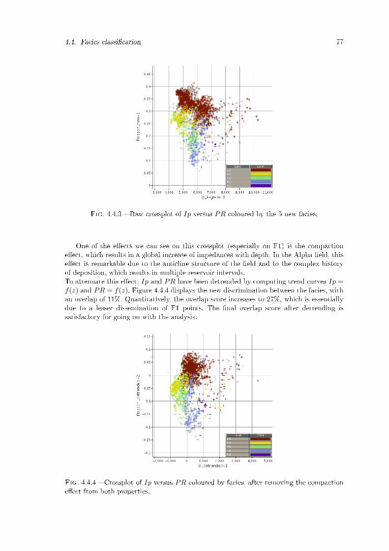
4.4. Facies classi�cation 77
Fig. 4.4.3 � Raw crossplot of Ip versus PR coloured by the 5 new facies.
One of the e�ects we can see on this crossplot (especially on F1) is the compactione�ect, which results in a global increase of impedances with depth. In the Alpha �eld, thise�ect is remarkable due to the anticline structure of the �eld and to the complex historyof deposition, which results in multiple reservoir intervals.To attenuate this e�ect, Ip and PR have been detrended by computing trend curves Ip =f(z) and PR = f(z). Figure 4.4.4 displays the new discrimination between the facies, withan overlap of 11%. Quantitatively, the overlap score increases to 27%, which is essentiallydue to a lesser dissemination of F1 points. The �nal overlap score after detrending issatisfactory for going on with the analysis.
Fig. 4.4.4 � Crossplot of Ip versus PR coloured by facies, after removing the compactione�ect from both properties.
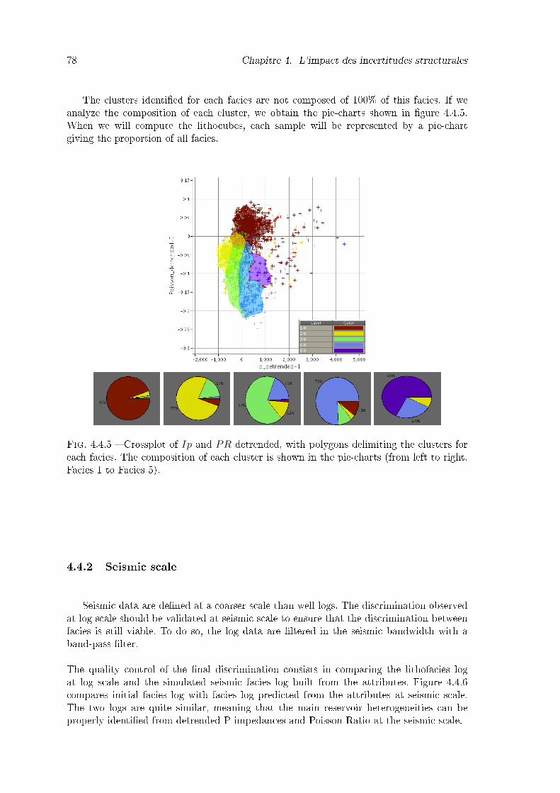
78 Chapitre 4. L'impact des incertitudes structurales
The clusters identi�ed for each facies are not composed of 100% of this facies. If weanalyze the composition of each cluster, we obtain the pie-charts shown in �gure 4.4.5.When we will compute the lithocubes, each sample will be represented by a pie-chartgiving the proportion of all facies.
Fig. 4.4.5 � Crossplot of Ip and PR detrended, with polygons delimiting the clusters foreach facies. The composition of each cluster is shown in the pie-charts (from left to right,Facies 1 to Facies 5).
4.4.2 Seismic scale
Seismic data are de�ned at a coarser scale than well logs. The discrimination observedat log scale should be validated at seismic scale to ensure that the discrimination betweenfacies is still viable. To do so, the log data are �ltered in the seismic bandwidth with aband-pass �lter.The quality control of the �nal discrimination consists in comparing the lithofacies logat log scale and the simulated seismic facies log built from the attributes. Figure 4.4.6compares initial facies log with facies log predicted from the attributes at seismic scale.The two logs are quite similar, meaning that the main reservoir heterogeneities can beproperly identi�ed from detrended P impedances and Poisson Ratio at the seismic scale.
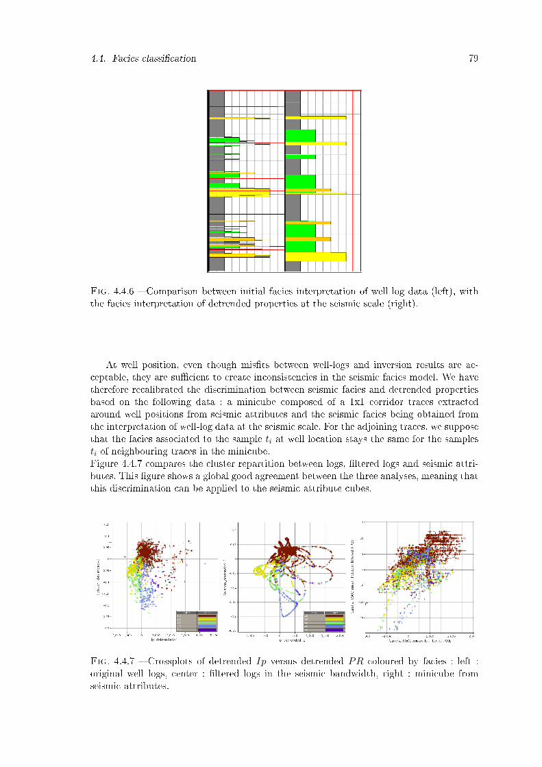
4.4. Facies classi�cation 79
Fig. 4.4.6 � Comparison between initial facies interpretation of well log data (left), withthe facies interpretation of detrended properties at the seismic scale (right).
At well position, even though mis�ts between well-logs and inversion results are ac-ceptable, they are su�cient to create inconsistencies in the seismic facies model. We havetherefore recalibrated the discrimination between seismic facies and detrended propertiesbased on the following data : a minicube composed of a 1x1 corridor traces extractedaround well positions from seismic attributes and the seismic facies being obtained fromthe interpretation of well-log data at the seismic scale. For the adjoining traces, we supposethat the facies associated to the sample ti at well location stays the same for the samplesti of neighbouring traces in the minicube.Figure 4.4.7 compares the cluster repartition between logs, �ltered logs and seismic attri-butes. This �gure shows a global good agreement between the three analyses, meaning thatthis discrimination can be applied to the seismic attribute cubes.
Fig. 4.4.7 � Crossplots of detrended Ip versus detrended PR coloured by facies : left :original well logs, center : �ltered logs in the seismic bandwidth, right : minicube fromseismic attributes.
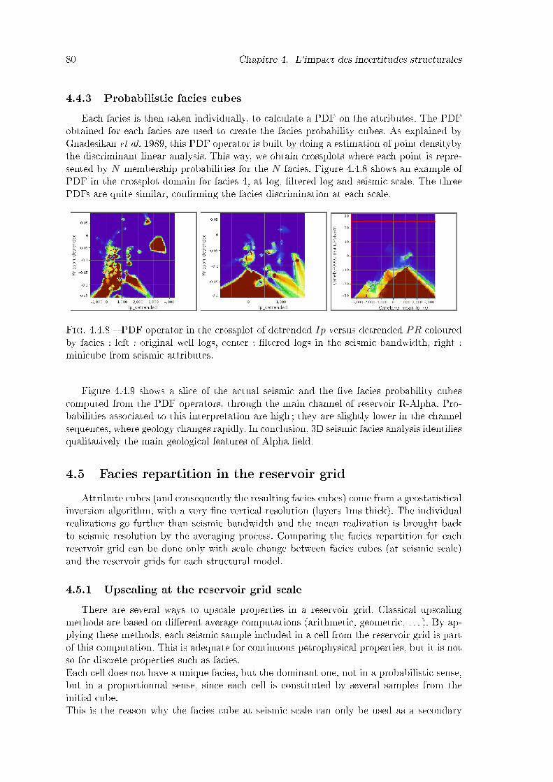
80 Chapitre 4. L'impact des incertitudes structurales
4.4.3 Probabilistic facies cubesEach facies is then taken individually, to calculate a PDF on the attributes. The PDF
obtained for each facies are used to create the facies probability cubes. As explained byGnadesikan et al. 1989, this PDF operator is built by doing a estimation of point densitybythe discriminant linear analysis. This way, we obtain crossplots where each point is repre-sented by N membership probabilities for the N facies. Figure 4.4.8 shows an example ofPDF in the crossplot domain for facies 4, at log, �ltered log and seismic scale. The threePDFs are quite similar, con�rming the facies discrimination at each scale.
Fig. 4.4.8 � PDF operator in the crossplot of detrended Ip versus detrended PR colouredby facies : left : original well logs, center : �ltered logs in the seismic bandwidth, right :minicube from seismic attributes.
Figure 4.4.9 shows a slice of the actual seismic and the �ve facies probability cubescomputed from the PDF operators, through the main channel of reservoir R-Alpha. Pro-babilities associated to this interpretation are high ; they are slightly lower in the channelsequences, where geology changes rapidly. In conclusion, 3D seismic facies analysis identi�esqualitatively the main geological features of Alpha �eld.
4.5 Facies repartition in the reservoir gridAttribute cubes (and consequently the resulting facies cubes) come from a geostatistical
inversion algorithm, with a very �ne vertical resolution (layers 1ms thick). The individualrealizations go further than seismic bandwidth and the mean realization is brought backto seismic resolution by the averaging process. Comparing the facies repartition for eachreservoir grid can be done only with scale change between facies cubes (at seismic scale)and the reservoir grids for each structural model.
4.5.1 Upscaling at the reservoir grid scaleThere are several ways to upscale properties in a reservoir grid. Classical upscaling
methods are based on di�erent average computations (arithmetic, geometric, . . . ). By ap-plying these methods, each seismic sample included in a cell from the reservoir grid is partof this computation. This is adequate for continuous petrophysical properties, but it is notso for discrete properties such as facies.Each cell does not have a unique facies, but the dominant one, not in a probabilistic sense,but in a proportionnal sense, since each cell is constituted by several samples from theinitial cube.This is the reason why the facies cube at seismic scale can only be used as a secondary
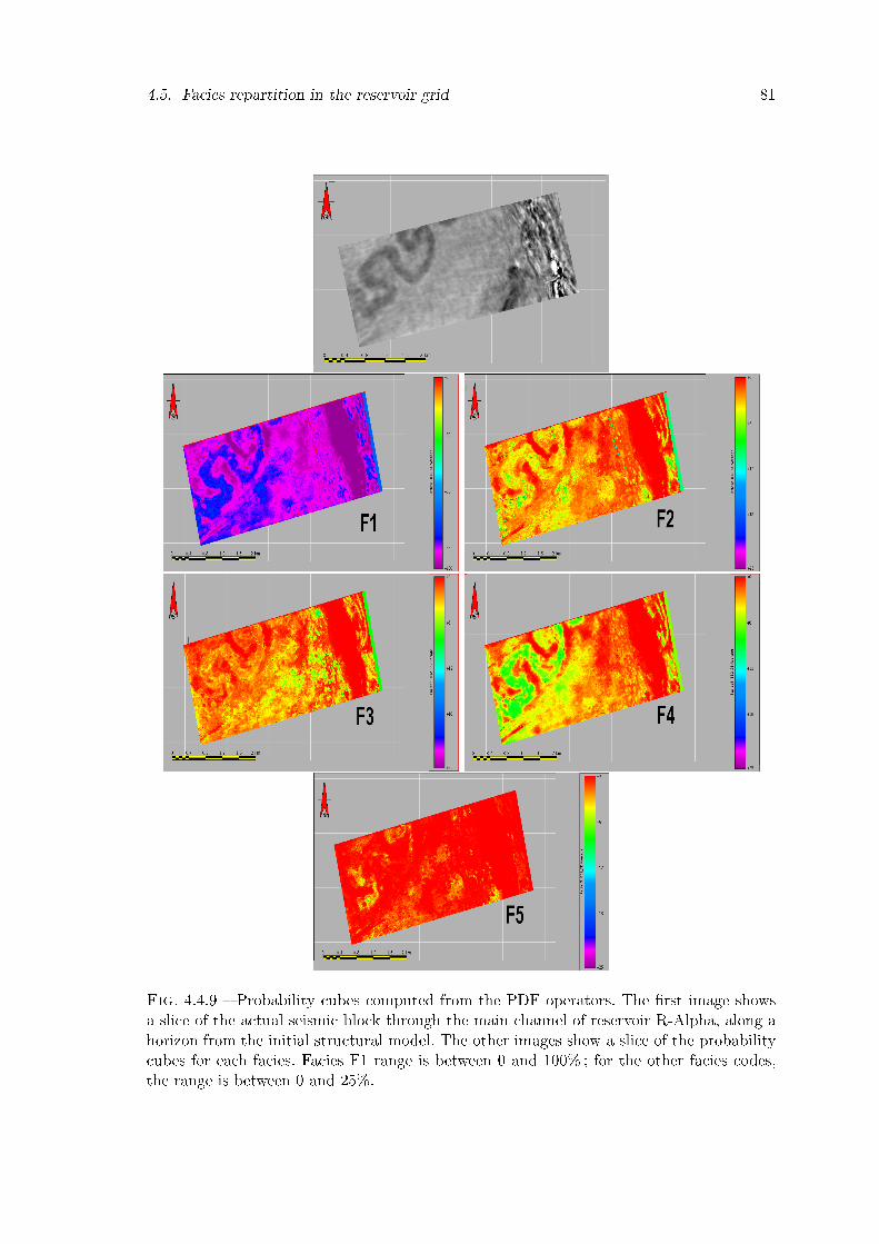
4.5. Facies repartition in the reservoir grid 81
Fig. 4.4.9 � Probability cubes computed from the PDF operators. The �rst image showsa slice of the actual seismic block through the main channel of reservoir R-Alpha, along ahorizon from the initial structural model. The other images show a slice of the probabilitycubes for each facies. Facies F1 range is between 0 and 100% ; for the other facies codes,the range is between 0 and 25%.
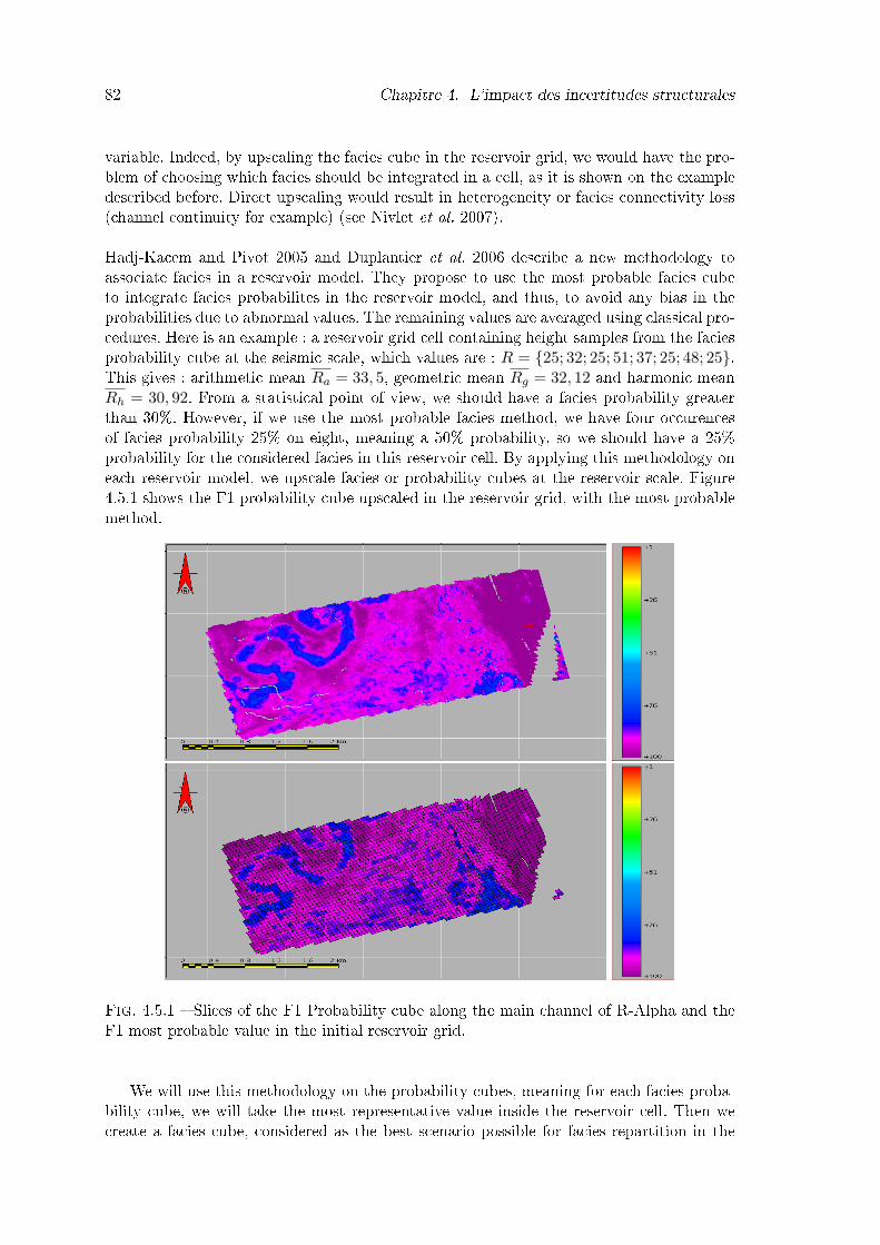
82 Chapitre 4. L'impact des incertitudes structurales
variable. Indeed, by upscaling the facies cube in the reservoir grid, we would have the pro-blem of choosing which facies should be integrated in a cell, as it is shown on the exampledescribed before. Direct upscaling would result in heterogeneity or facies connectivity loss(channel continuity for example) (see Nivlet et al. 2007).Hadj-Kacem and Pivot 2005 and Duplantier et al. 2006 describe a new methodology toassociate facies in a reservoir model. They propose to use the most probable facies cubeto integrate facies probabilites in the reservoir model, and thus, to avoid any bias in theprobabilities due to abnormal values. The remaining values are averaged using classical pro-cedures. Here is an example : a reservoir grid cell containing height samples from the faciesprobability cube at the seismic scale, which values are : R = {25; 32; 25; 51; 37; 25; 48; 25}.This gives : arithmetic mean Ra = 33, 5, geometric mean Rg = 32, 12 and harmonic meanRh = 30, 92. From a statistical point of view, we should have a facies probability greaterthan 30%. However, if we use the most probable facies method, we have four occurencesof facies probability 25% on eight, meaning a 50% probability, so we should have a 25%probability for the considered facies in this reservoir cell. By applying this methodology oneach reservoir model, we upscale facies or probability cubes at the reservoir scale. Figure4.5.1 shows the F1 probability cube upscaled in the reservoir grid, with the most probablemethod.
Fig. 4.5.1 � Slices of the F1 Probability cube along the main channel of R-Alpha and theF1 most probable value in the initial reservoir grid.
We will use this methodology on the probability cubes, meaning for each facies proba-bility cube, we will take the most representative value inside the reservoir cell. Then wecreate a facies cube, considered as the best scenario possible for facies repartition in the
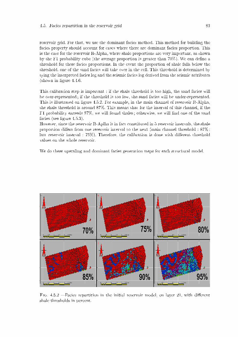
4.5. Facies repartition in the reservoir grid 83
reservoir grid. For that, we use the dominant facies method. This method for building thefacies property should account for cases where there are dominant facies proportion. Thisis the case for the reservoir R-Alpha, where shale proportions are very important, as shownby the F1 probability cube (the average proportion is greater than 70%). We can de�ne athreshold for these facies proportions. In the event the proportion of shale falls below thethreshold, one of the sand facies will take over in the cell. This threshold is determined bytying the interpreted facies log and the seismic facies log derived from the seismic attributes(shown in �gure 4.4.6.This calibration step is important : if the shale threshold is too high, the sand facies willbe over-represented ; if the threshold is too low, the sand facies will be under-represented.This is illustrated on �gure 4.5.2. For example, in the main channel of reservoir R-Alpha,the shale threshold is around 87%. This means that for the interval of this channel, if theF1 probability exceeds 87%, we will found shales ; otherwise, we will �nd one of the sandfacies (see �gure 4.5.3).However, since the reservoir R-Aplha is in fact constituted in 5 reservoir intervals, the shaleproportion di�ers from one reservoir interval to the next (main channel threshold : 87% ;last reservoir interval : 75%). Therefore, the calibration is done with di�erent thresholdvalues on the whole reservoir.We do these upscaling and dominant facies generation steps for each structural model.
Fig. 4.5.2 � Facies repartition in the initial reservoir model, on layer 21, with di�erentshale thresholds in percent.
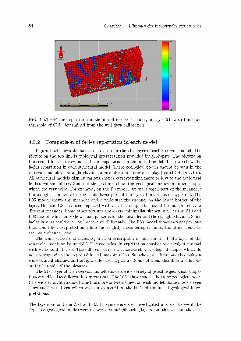
84 Chapitre 4. L'impact des incertitudes structurales
Fig. 4.5.3 � Facies repartition in the initial reservoir model, on layer 21, with the shalethreshold of 87%, determined from the well data calibration.
4.5.2 Comparison of facies repartition in each modelFigure 4.5.4 shows the facies repartition for the 21st layer of each reservoir model. The
picture on the top line is geological interpretation provided by geologists. The picture onthe second line, left row, is the facies repartition for the initial model. Then we show thefacies repartition in each structural model. Three geological bodies should be seen in thereservoir models : a straight channel, a meander and a crevasse splay (noted CS hereafter).All structural models display various shapes corresponding more or less to the geologicalbodies we should see. Some of the pictures show the geological bodies or other shapeswhich are very wide. For example, on the P0 model, we see a small part of the meander ;the straight channel takes the whole lower part of the layer ; the CS has disappeared. TheP05 model shows the meander and a wide straight channel on the lower border of thelayer. But the CS has been replaced with a U-like shape that could be interpreted as adi�erent meander. Some other pictures show very minimalist shapes, such as the P10 andP90 models which only show small patterns for the meander and the straight channel. Somefacies layouts could even be interpreted di�erently. The P50 model shows two shapes, onethat could be interpreted as a �ne and slightly meandering channel, the other could beseen as a channel lobe.
The same exercise of facies repartition description is done for the 105th layer of thereservoir models on �gure 4.5.5. The geological interpretation consists of a straight channelwith wide sandy levees. The di�erent structural models show geological shapes which donot correspond to the expected initial interpretation. Somehow, all these models display awide straight channel on the right side of each picture. Some of them also show a side lobeon the left side of the pictures.
The 21st layer of the reservoir models shows a wide variety of possible geological shapesthat would lead to di�erent interpretations. The 105th layer shows the same geological body(the wide straight channel) which is more or less de�ned on each model. Some models evenshow another pattern which was not expected on the basis of the initial geological inter-pretations.The layers around the 21st and 105th layers were also investigated in order to see if theexpected geological bodies were recovered on neighbouring layers, but this was not the case
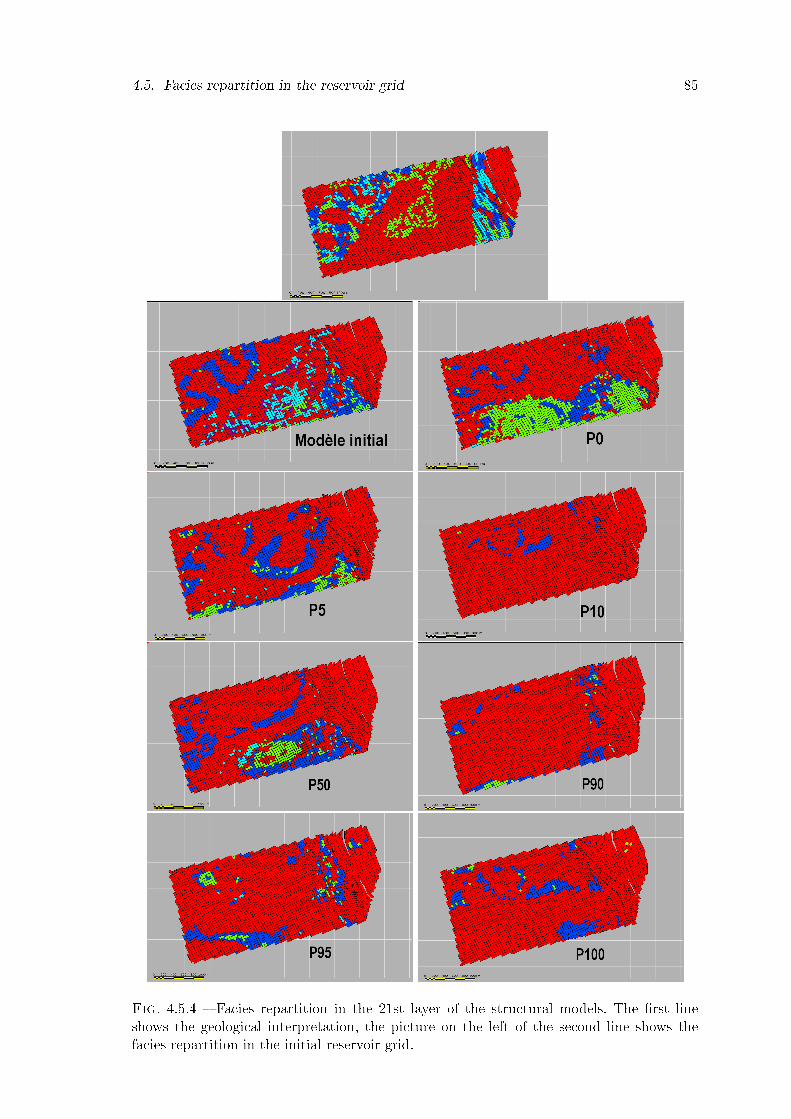
4.5. Facies repartition in the reservoir grid 85
Fig. 4.5.4 � Facies repartition in the 21st layer of the structural models. The �rst lineshows the geological interpretation, the picture on the left of the second line shows thefacies repartition in the initial reservoir grid.
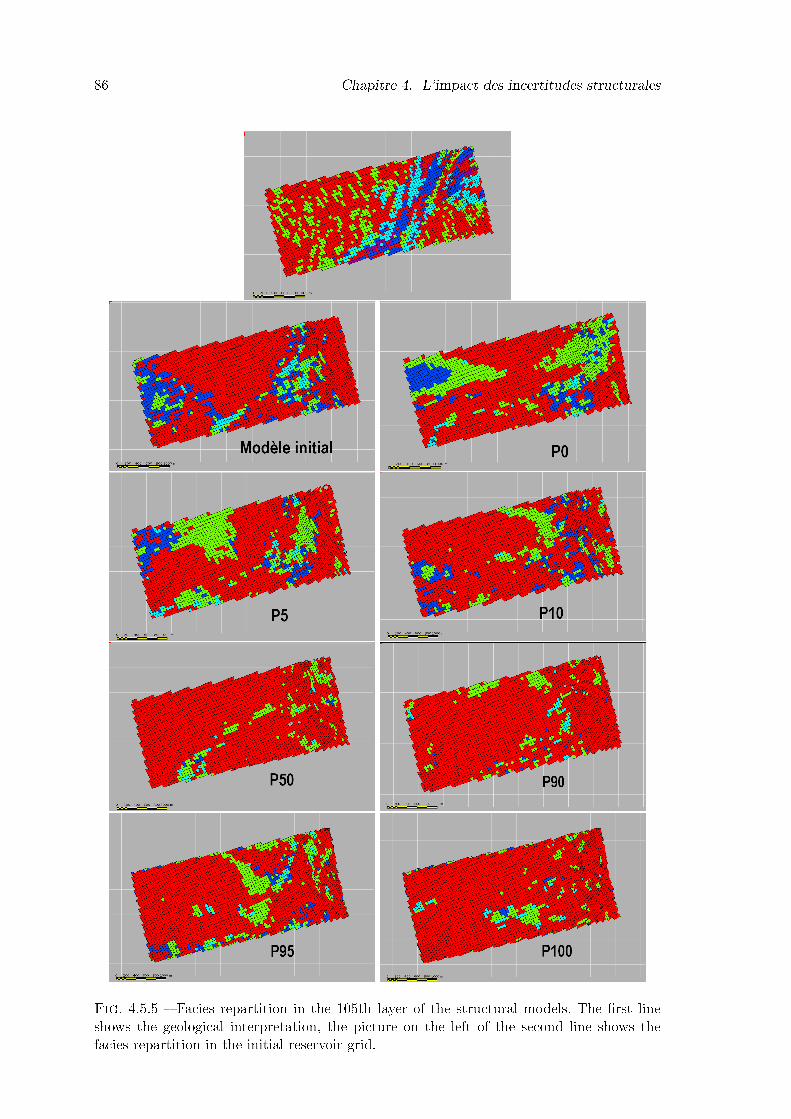
86 Chapitre 4. L'impact des incertitudes structurales
Fig. 4.5.5 � Facies repartition in the 105th layer of the structural models. The �rst lineshows the geological interpretation, the picture on the left of the second line shows thefacies repartition in the initial reservoir grid.
4.6. Conclusion 87
for both of them.
4.6 ConclusionAn important issue in understanding heterogeneous reservoirs is determining the rela-
tive importance of structural and petrophysical variability. Structural uncertainty is nottypically incorporated into the construction of a reservoir model, unlike petrophysical un-certainty.We have presented a simple methodology to evaluate their e�ects in a reservoir model.This methodology is based on using 3D reservoir grids. Multiple realizations of structuralmodels have been simulated and used in a standard reservoir modeling work�ow. For eachreservoir grid, we obtain the facies repartition and systematically investigate it. Each modelshows di�erent facies layouts with diverse possible geological interpretations.The results further reveal that evaluating the structural uncertainty e�ects in reservoirgrids is an important step before choosing the de�nitive model to be used in future studies.By visualizing the structural uncertainty, we can gain a greater appreciation of the re-liability of any analysis performed in reservoir characterization studies. Structural uncer-tainties are quanti�able and can be carried through a reservoir characterization work�owby building several reservoir models. The example shown here with the Alpha �eld de-monstrates how structural uncertainty can lead to di�erent facies repartition and to wronginterpretation in the reservoir models.


Partie II
Alternatives à l'approche
directe
89

Chapitre 5
Inversion par déformation graduelle
5.1 IntroductionUne étude réservoir a pour objectif �nal la création d'un modèle nous permettant de
prédire dans le futur le comportement du réservoir au cours de sa production. Pour prédireles propriétés pétrophysiques qui nous permettront de faire cette simulation, nous cher-chons à intégrer autant d'information que possible dans le réservoir.Les méthodes traditionnelles de simulation réservoir créent un modèle de lithotype (envi-ronnement + faciès géologiques + propriétés pétrophysiques) :
� par des techniques "objet" : processus booléens, modélisation d'objets longs, pro-cessus génétiques ;
� par des techniques "pixel" : simulations gaussiennes, simulation d'indicatrice, sta-tistiques multipoints.
Les modèles réservoirs résultants de ces processus sont conditionnés aux puits, mais laté-ralement, nous n'avons aucune certitude sur leur validité.Les méthodes traditionnelles de caractérisation réservoir font appels aux données sismiquespour contraindre le réservoir. Les données sismiques sont la seule source d'information quicouvre l'intégralité du réservoir. Elles sont l'expression des contrastes des propriétés pétroé-lastiques aux limites des couches géologiques. Les valeurs réelles des propriétés ne sont doncpas connues dans l'absolue. Un second problème est que les attributs dérivés des donnéessismiques sont à une échelle di�érente de celle du réservoir, et il faut donc soit e�ectuerun changement d'échelle de ces attributs (upscaling), avec tous les problèmes associés à cechangement d'échelle (Ringrose 2007), soit simuler les propriétés réservoirs en se servantdes attributs comme variables secondaires.Nous proposons une nouvelle méthode d'inversion à mi-chemin entre les disciplines simula-tion réservoir et caractérisation sismique du réservoir. Ce processus d'inversion permet degénérer des attributs sismiques directement à l'échelle réservoir. Il est basé sur le couplagede deux techniques :
� les déformations graduelles, pour la génération de réalisations géostatistiques d'at-tributs ;
� la modélisation sismique, pour l'optimisation à partir des données sismiques.
Le processus d'inversion proposé suit le schéma suivant :1. Combinaisons des réalisations de propriétés suivant le principe de fonctionnement
des déformations graduelles
91

92 Chapitre 5. Inversion par déformation graduelle
2. Introduction de l'information géologique fournie par les données de puits commecontraintes
3. Création d'un volume sismique synthétique à partir des nouvelles réalisations4. Minimisation de la fonction coût basée sur les volumes sismiques réels et synthétiques5. Itération jusqu'à satisfaction.Ce schéma de fonctionnement est illustré sur la �gure 5.1.1. Il di�ère des inversions
traditionnelles dans le sens où la simulation des propriétés se fait directement à l'échelleréservoir, et que la comparaison se fait à l'échelle sismique (Neau et al. 2008).
Fig. 5.1.1 � Schéma de fonctionnement des déformations graduelles.
5.2 Principe de fonctionnement des déformations graduellesLes simulations géostatistiques nous fournissent de multiples réalisations de propriétés
réservoirs qui reproduisent les statistiques obtenues des données disponibles, mais dans laplupart des cas, elles ne re�ètent pas la réalité de ces données. Par exemple, les statistiquesdes propriétés d'un chenal n'assureront pas la reproduction de la forme du chenal dans unesimulation.
Traditionnellement, le réservoir est ajusté sur la base des données de production pardes méthodes sophistiquées de calage historique (history matching). La création des mo-dèles réservoirs pour ce processus est basée principalement sur deux types de méthodes. Lapremière consiste à construire des réalisations de modèles conditionnées aux observationsen utilisant par exemple la méthode de Monte Carlo et Chaînes de Markov. Mais cette ap-proche est coûteuse en temps de calcul. Une autre approche est basée sur des méthodes quiutilisent un nombre limité de paramètres pour calibrer les modèles aux données observées,comme par exemple la méthode des points pilotes. Mais ce genre d'approche ne fonctionnepas pour des problèmes de dimension élevée comme une grille réservoir.
5.2. Principe de fonctionnement des déformations graduelles 93
Les déformations graduelles ont donc été développées pour dépasser les problèmes de tempsd'exécution d'une part, et la dimension du réservoir d'autre part. Les déformations gra-duelles sont donc d'un outil capable de modi�er les réalisations de propriétés réservoirs,tout en maintenant les contraintes aux données géologiques et en reproduisant un com-portement connu (les données dynamiques pour l'utilisation courante des déformationsgraduelles, les données sismiques dans l'application décrite ici), tout en ayant un tempsd'exécution raisonnable, et s'appliquant à tous types de modèles, quelle que soit sa taille.En utilisant un mécanisme simple de perturbation des réalisations, la méthode des défor-mations graduelles cherche dans l'espace du modèle a priori les solutions qui honorent lesdonnées que l'on veut inverser. Ce mécanisme assure le respect des statistiques du modèle(Caers 2007).
5.2.1 Formulation de baseLes déformations graduelles sont donc une méthode de reparamètrisation géostatistique,
dont l'hypothèse de base est de considérer le réservoir comme un processus spatio-temporel.Plusieurs formulations existent mais elles s'appuient toutes sur l'idée suivante : "la sommede deux fonctions aléatoires gaussiennes est une fonction aléatoire gaussienne" (Hu 2000)formulée par :
Y (t) = Y0.cos(t) + Y1.sin(t) (5.1)avec Y la réalisation optimale, Y0 la réalisation initiale, Y1 la réalisation secondaire et t lecoe�cient de déformation graduelle.Cette combinaison linéaire conserve le comportement gaussien des éléments Y , Y0 et Y1 del'équation. Y0 et Y1 sont dé�nies comme des réalisations ayant des statistiques similaires(moyenne et covariance). En faisant varier le paramètre t tel que t ∈ D =
[0 ; π
2
], nousgénérons une chaîne continue de réalisations allant de Y0 (quand t = 0)à Y1 (quand t = π
2 ),se déformant graduellement de l'une à l'autre pour des valeurs intermédiaires, tel quemontré sur la �gure 5.2.1. Une fois que cette chaîne de réalisations est disponible, onminimise une fonction coût en fonction du paramètre t.Comme évoqué dans le schéma 5.1.1, cette procédure est appliquée de manière itérativepour permettre de diminuer la fonction coût à un niveau satisfaisant. Ceci nous donnel'équation suivante :
Yn(t) = Yn−1.cos(t) + Un.sin(t) (5.2)avec Yn la réalisation optimale à l'itération n, Yn−1 la réalisation optimale de l'étape
précédente et Un la réalisation secondaire de l'itération n.Les méthodes statistiques sont largement utilisées pour modéliser des propriétés réservoirsdistribuées dans l'espace. Dans de nombreux cas, il n'y a pas su�samment de donnéespour en déduire avec précision les paramètres structuraux d'un modèle stochastique. Cesparamètres, qui dé�nissent la géométrie des corps, sont souvent exprimés par des distri-butions a priori et des variogrammes. La simulation doit donc inclure un paramètre surlequel repose tout cet aspect structural, découplé de la simulation de la distribution de lapropriété. Prenons L l'opérateur covariance et X un bruit blanc gaussien standard. On aalors :
Yn = L [Xn] (5.3)
94 Chapitre 5. Inversion par déformation graduelle
Ceci nous donne une réalisation gaussienne Y dont la covariance impose la structurespatiale de la réalisation. Appliqué à la formulation des déformations graduelles, nousavons :
Yn(L, t) = L[Xn(t)] = L [Yn−1.cos(t) + Un.sin(t)] (5.4)Sous cette forme, on peut donc appliquer les déformations graduelles sur les réalisations
tout en modi�ant la fonction de covariance (voir �gure 5.2.1). Cette formulation correspondaux déformations graduelles structurales.
Dans d'autres cas, il peut être utile de ne modi�er qu'une partie du modèle réservoir.En e�et, pour un réservoir déjà étudié, des changements locaux, liés à des données récem-ment acquises, peuvent s'avérer nécessaires. Reprendre l'étude du réservoir depuis le débutserait long et fastidieux, et le fait de réajuster une zone par le processus global pourraitdégrader la qualité d'une autre zone. Il existe une formulation des déformations graduellesqui permet d'appliquer des modi�cations locales dans le modèle réservoir. Ces modi�ca-tions ne peuvent s'appliquer que si la réalisation secondaire prend elle-même en comptel'aspect local de la modi�cation.Ravalec-Dupin et al. 2000 ont donc proposé une formulation particulière de simulationFFT, appelée FFTMA (pour Fast Fourier Transform Moving Average). Cette formulationpermet de considérer X le bruit blanc de tout le modèle réservoir par {X1, . . . , Xn} lapartition de X en n zones indépendantes. Chaque zone peut donc être manipulée indi-viduellement. Il se pose alors un problème de continuité spatiale entre les zones. Mais lesdéformations graduelles locales s'appliquent uniquement sur le champ de bruit blanc. Ainsi,en appliquant la fonction de covariance, sur le bruit blanc modi�é, la continuité spatialede la propriété est préservée (comme montré sur la �gure 5.2.1).
5.2.2 Génération des réalisations secondairesLe processus de déformation graduelle nécessite de générer une réalisation secondaire
complémentaire indépendante de la réalisation initiale, mais ayant les mêmes statistiques(moyenne, variance, covariance).Hu et al. 1999 ont comparé plusieurs méthodes de simulation géostatistiques pour obtenirces réalisations secondaires. L'applicabilité des méthodes comparées est focalisée sur l'uti-lisation des trois formulations des déformations graduelles. Mais seule une méthode retientl'attention : la Transformée de Fourier Rapide en Moyenne Mobile (FFTMA). Cette mé-thode de simulation est retenue pour sa rapidité, son aptitude à découpler la générationdes nombres aléatoires et les paramètres structuraux et sa capacité à découper le modèleréservoir en zone.Cette méthode est basée sur le principe de génération de champs aléatoires gaussiens parméthode spectrale (voir Li and Kareem 1991 et Ruan and McLaughlin 1998). La formula-tion est brièvement rappelée ci-après.
La méthode de moyenne mobile permet de générer des réalisations gaussiennes y demoyenne µ et covariance C, considérée comme une matrice. La réalisation y est obtenuepar :
y = µ+ g ⊗ z (5.5)
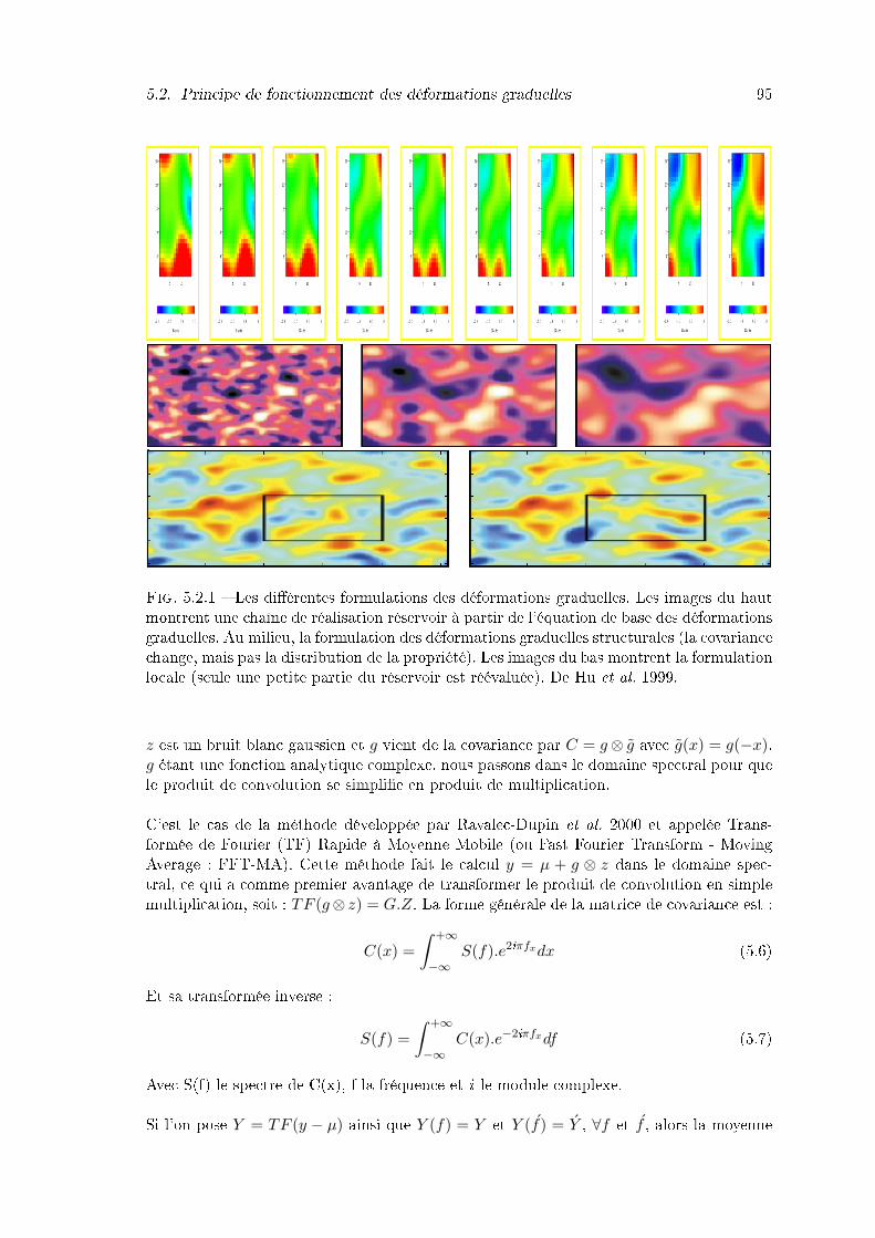
5.2. Principe de fonctionnement des déformations graduelles 95
Fig. 5.2.1 � Les di�érentes formulations des déformations graduelles. Les images du hautmontrent une chaîne de réalisation réservoir à partir de l'équation de base des déformationsgraduelles. Au milieu, la formulation des déformations graduelles structurales (la covariancechange, mais pas la distribution de la propriété). Les images du bas montrent la formulationlocale (seule une petite partie du réservoir est réévaluée). De Hu et al. 1999.
z est un bruit blanc gaussien et g vient de la covariance par C = g⊗ g avec g(x) = g(−x).g étant une fonction analytique complexe, nous passons dans le domaine spectral pour quele produit de convolution se simpli�e en produit de multiplication.C'est le cas de la méthode développée par Ravalec-Dupin et al. 2000 et appelée Trans-formée de Fourier (TF) Rapide à Moyenne Mobile (ou Fast Fourier Transform - MovingAverage : FFT-MA). Cette méthode fait le calcul y = µ + g ⊗ z dans le domaine spec-tral, ce qui a comme premier avantage de transformer le produit de convolution en simplemultiplication, soit : TF (g⊗ z) = G.Z. La forme générale de la matrice de covariance est :
C(x) =∫ +∞
−∞S(f).e2iπfxdx (5.6)
Et sa transformée inverse :
S(f) =∫ +∞
−∞C(x).e−2iπfxdf (5.7)
Avec S(f) le spectre de C(x), f la fréquence et i le module complexe.Si l'on pose Y = TF (y − µ) ainsi que Y (f) = Y et Y (f) = Y , ∀f et f , alors la moyenne
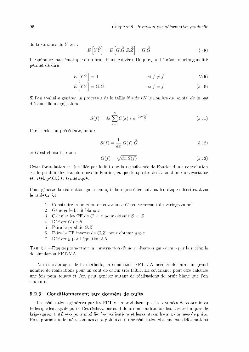
96 Chapitre 5. Inversion par déformation graduelle
de la variance de Y est :E
[Y
¯Y
]= E
[G.
¯G.Z.
¯Z
]= G.
¯G (5.8)
L'espérance mathématique d'un bruit blanc est zéro. De plus, le théorème d'orthogonalitépermet de dire :
E[Y
¯Y
]= 0 si f 6= f (5.9)
E[Y
¯Y
]= G.
¯G si f = f (5.10)
Si l'on souhaite générer un processus de la taille N ∗ dx (N le nombre de points, dx le pasd'échantillonnage), alors :
S(f) = dxN∑
x=1
C(x) ∗ e−2iπ xfN (5.11)
Par la relation précédente, on a :
S(f) =1dx.G(f). ¯G (5.12)
et G est choisi tel que :G(f) =
√dx.S(f) (5.13)
Cette formulation est justi�ée par le fait que la transformée de Fourier d'une convolutionest le produit des transformées de Fourier, et que le spectre de la fonction de covarianceest réel, positif et symétrique.Pour générer la réalisation gaussienne, il faut procéder suivant les étapes décrites dansle tableau 5.1.
1 Construire la fonction de covariance C (en se servant du variogramme)2 Générer le bruit blanc z3 Calculer les TF de C et z pour obtenir S et Z4 Dériver G de S5 Faire le produit G.Z6 Faire la TF inverse de G.Z, pour obtenir g ⊗ z7 Dériver y par l'équation 5.5
Tab. 5.1 � Etapes permettant la construction d'une réalisation gaussienne par la méthodede simulation FFT-MA.
Autres avantages de la méthode, la simulation FFT-MA permet de faire un grandnombre de réalisations pour un coût de calcul très faible. La covariance peut être calculéeune fois pour toutes et l'on peut générer autant de réalisations de bruit blanc que l'onsouhaite.
5.2.3 Conditionnement aux données de puitsLes réalisations générées par les FFT ne reproduisent pas les données de contraintes
telles que les logs de puits. Ces réalisations sont donc non conditionnelles. Des techniques dekrigeage sont utilisées pour modi�er les réalisations et les contraindre aux données de puits.En supposant n données connues en n points et Y une réalisation obtenue par déformations

5.3. Optimisation et itération du processus 97
graduelles, Y est conditionnée aux données par la relation suivante (Chiles and Del�ner1999) :
Yc(u) = Ydk(u) + [Y (u)− Yk(u)] (5.14)avec u le point objectif, Yc la réalisation conditionnée, Ydk l'estimation par krigeage desdonnées connues et Yk l'estimation par krigeage de la réalisation non conditionnée. Lesestimations par krigeage Xk sont réalisées par :
Xk(u) =n∑
i=1
λi(u)X(ui) (5.15)
avec λi le poids associés à chaque point de données ui, que l'on dérive de Cλ = B, où C estl'opérateur covariance (le même que celui utilisé pour les déformations graduelles) et B estun vecteur de corrélation spatiale entre la valeur à estimer en u et l'observation aux pointui. Cette formulation nous permet de ramener la réalisation non conditionnelle à zéro etd'ajouter ensuite les données connues, tout en respectant la structure spatiale (voir �gure5.2.2).
Fig. 5.2.2 � Principe du krigeage des réalisations non conditionnées dans le processusdes déformations graduelles. La ligne 1 représente la simulation non-conditionnée avec lepoint de données et l'estimation par krigeage du point ; la ligne 2 montre la simulationconditionnée.
5.3 Optimisation et itération du processusLe processus complet d'inversion par déformation graduelle est basé sur un schéma
itératif implémenté à partir de l'équation 5.2 pour que la fonction coût puisse décroîtrejusqu'à un niveau jugé satisfaisant. Nous regardons maintenant comment la fonction coûtest optimisée par itération.
5.3.1 Optimisation dans l'espace de rechercheL'équation 5.2 s'apparente à la recherche d'un point optimum dans un espace de di-
mension N (la dimension du modèle réservoir en nombre de cellule). Comme le montre Huand Ravalec-Dupin 2004, la chaîne de réalisations construite en faisant varier t explore ledomaine d'existence de la propriétés à simuler. La chaîne de réalisations décrit donc une

98 Chapitre 5. Inversion par déformation graduelle
hyperellipse de dimension N .Pour illustrer ce phénomène, prenons un exemple de modèle réservoir à deux cellules, avecY1 la réalisation initiale et Y2 la réalisation secondaire, de moyenne Y0 et covariance iden-tiques :
Y1 ={
a1
b1
}, Y2 =
{a2
b2
}(5.16)
Le principe de déformation graduelle nous donne :Y3(t) = Y1.cos(t) + Y2.sin(t) (5.17){
a3(t)b3(t)
}=
{a1
b1
}cos(t) +
{a2
b2
}sin(t) (5.18)
Cette équation s'apparente à la paramètrisation cartésienne d'une ellipse en deux di-mensions : {
x = α.cos(t)y = β.sin(t)
(5.19)Cela signi�e que Y1, Y2 et Y3 sont des points de cette ellipse, et que, en faisant varier
t, alors Y1, Y2 et Y3 se déplace le long de l'ellipse (voir �gure 5.3.1). L'ellipse ne décritqu'une petite partie de l'espace de recherche. Il est donc peu probable que la solution setrouve sur cette ellipse. Le processus d'optimisation doit donc être répété. Cela revient àcréer une suite d'ellipses reliées les unes aux autres par la réalisation optimale de chaqueitération (qui devient la réalisation initiale de l'itération suivante), et qui converge vers unpoint de l'espace qui correspond à la solution. La représentation en deux dimensions de cephénomène est illustrée sur la �gure 5.3.1.
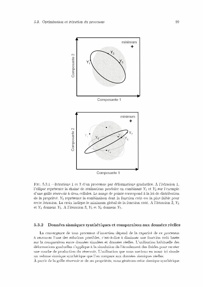
5.3. Optimisation et itération du processus 99
Fig. 5.3.1 � Itérations 1 et 3 d'un processus par déformations graduelles. A l'itération 1,l'ellipse représente la chaîne de réalisations produite en combinant Y1 et Y2 sur l'exempled'une grille réservoir à deux cellules. Le nuage de points correspond à la loi de distributionde la propriété. Y3 représente la combinaison dont la fonction coût est la plus faible pourcette itération. La croix indique le minimum global de la fonction coût. A l'itération 2, Y3
et Y4 donnent Y5. A l'itération 3, Y5 et Y6 donnent Y7.
5.3.2 Données sismiques synthétiques et comparaison aux données réellesLa convergence de tout processus d'inversion dépend de la capacité de ce processus
à retrouver l'une des solutions possibles, c'est-à-dire à diminuer une fonction coût baséesur la comparaison entre données simulées et données réelles. L'utilisation habituelle desdéformations graduelles s'applique à la simulation de l'écoulement des �uides pour recréerune courbe de production du réservoir. L'utilisation que nous mettons en avant ici simuleun volume sismique synthétique que l'on compare aux données sismiques réelles.À partir de la grille réservoir et de ses propriétés, nous générons cette sismique synthétique
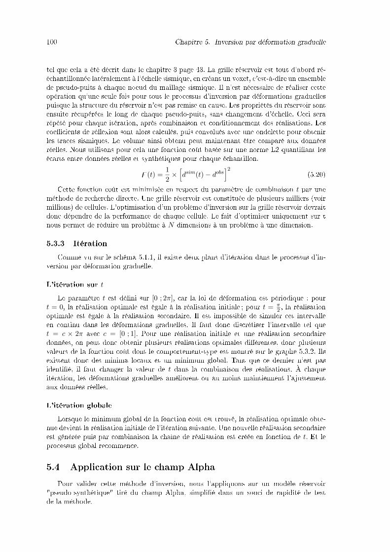
100 Chapitre 5. Inversion par déformation graduelle
tel que cela a été décrit dans le chapitre 3 page 43. La grille réservoir est tout d'abord ré-échantillonnée latéralement à l'échelle sismique, en créant un voxet, c'est-à-dire un ensemblede pseudo-puits à chaque noeud du maillage sismique. Il n'est nécessaire de réaliser cetteopération qu'une seule fois pour tout le processus d'inversion par déformations graduellespuisque la structure du réservoir n'est pas remise en cause. Les propriétés du réservoir sontensuite récupérées le long de chaque pseudo-puits, sans changement d'échelle. Ceci serarépété pour chaque itération, après combinaison et conditionnement des réalisations. Lescoe�cients de ré�exion sont alors calculés, puis convolués avec une ondelette pour obtenirles traces sismiques. Le volume ainsi obtenu peut maintenant être comparé aux donnéesréelles. Nous utilisons pour cela une fonction coût basée sur une norme L2 quanti�ant lesécarts entre données réelles et synthétiques pour chaque échantillon.
z(t) =12×
[dsim(t)− dobs
]2 (5.20)Cette fonction coût est minimisée en respect du paramètre de combinaison t par une
méthode de recherche directe. Une grille réservoir est constituée de plusieurs milliers (voirmillions) de cellules. L'optimisation d'un problème d'inversion sur la grille réservoir devraitdonc dépendre de la performance de chaque cellule. Le fait d'optimiser uniquement sur tnous permet de réduire un problème à N dimensions à un problème à une dimension.
5.3.3 ItérationComme vu sur le schéma 5.1.1, il existe deux plans d'itération dans le processus d'in-
version par déformation graduelle.L'itération sur t
Le paramètre t est dé�ni sur [0 ; 2π], car la loi de déformation est périodique : pourt = 0, la réalisation optimale est égale à la réalisation initiale ; pour t = π
2 , la réalisationoptimale est égale à la réalisation secondaire. Il est impossible de simuler cet intervalleen continu dans les déformations graduelles. Il faut donc discrétiser l'intervalle tel quet = c × 2π avec c = [0 ; 1]. Pour une réalisation initiale et une réalisation secondairedonnées, on peut donc obtenir plusieurs réalisations optimales di�érentes, donc plusieursvaleurs de la fonction coût dont le comportement-type est montré sur le graphe 5.3.2. Ilsexistent donc des minima locaux et un minimum global. Tant que ce dernier n'est pasidenti�é, il faut changer la valeur de t dans la combinaison des réalisations. À chaqueitération, les déformations graduelles améliorent ou au moins maintiennent l'ajustementaux données réelles.L'itération globale
Lorsque le minimum global de la fonction coût est trouvé, la réalisation optimale obte-nue devient la réalisation initiale de l'itération suivante. Une nouvelle réalisation secondaireest générée puis par combinaison la chaîne de réalisation est créée en fonction de t. Et leprocessus global recommence.
5.4 Application sur le champ AlphaPour valider cette méthode d'inversion, nous l'appliquons sur un modèle réservoir
"pseudo-synthétique" tiré du champ Alpha, simpli�é dans un souci de rapidité de testde la méthode.

5.4. Application sur le champ Alpha 101
Fig. 5.3.2 � Comportement type de la fonction coût pendant une itération donnée, enfonction de c. En c = 0, nous avons la réalisation initiale, en c = 1 la réalisation secondaire.En c = 0.05, on note un minima local de la fonction coût et en c = 0.95, le minima global(en rouge) qui correspond à la réalisation optimale de l'itération.
5.4.1 Le modèle initial
Une petite grille réservoir est extraite du modèle original, en prenant soin que cettemini grille contienne le puits. Nous faisons le choix d'extraire cette mini grille avec unefaible dimension latérale, et la dimension verticale complète de la grille d'origine, soit26 × 26 × 113 = 76388 cellules. Le puits traverse cette grille, ce qui nous donne, pourchaque couche du modèle, un point de conditionnement par couche (voir �gure 5.4.1).
Au lieu de réaliser une inversion en impédance, nous faisons une inversion en vitesseP et densité pour voir la capacité de l'inversion par déformations graduelles à récupérerces propriétés. Le modèle initial (Y0 dans la formulation de base) est généré à partir del'interprétation géologique du champ Alpha : des faciès ont été reportés dans la grilleréservoir, et à l'aide du modèle pétroélastique, nous créons les propriétés vitesse P etdensité. Nous calculons les lois d'enfouissement pour les logs de chaque propriété (densité,vitesse P) et pour chaque faciès (voir �gure 5.4.2. Ces lois sont ensuite appliquées pourtoute la grille réservoir.
La �gure 5.4.3 montrent trois couches du réservoir pour la vitesse P (notée Vp). Leshistogrammes de ces propriétés initiales en �gure 5.4.4 servent à passer dans le domainegaussien par anamorphose. La sismique " initiale", créée à partir de ces propriétés, estmontrée en �gure 5.4.16. On peut remarquer que les données synthétiques du modèleinitial ressemblent peu à de la sismique. À l'exception de la trajectoire du puits sur lequelle modèle pétroélastique s'appuie, le modèle est très peu réaliste et montre un manque�agrant de variabilité dans les propriétés associées aux argiles.
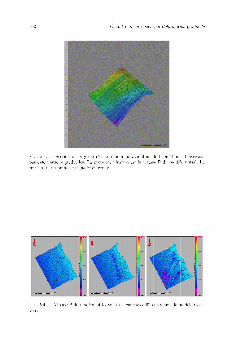
102 Chapitre 5. Inversion par déformation graduelle
Fig. 5.4.1 � Section de la grille réservoir pour la validation de la méthode d'inversionpar déformations graduelles. La propriété illustrée est la vitesse P du modèle initial. Latrajectoire du puits est signalée en rouge.
Fig. 5.4.3 � Vitesse P du modèle initial sur trois couches di�érentes dans le modèle réser-voir.
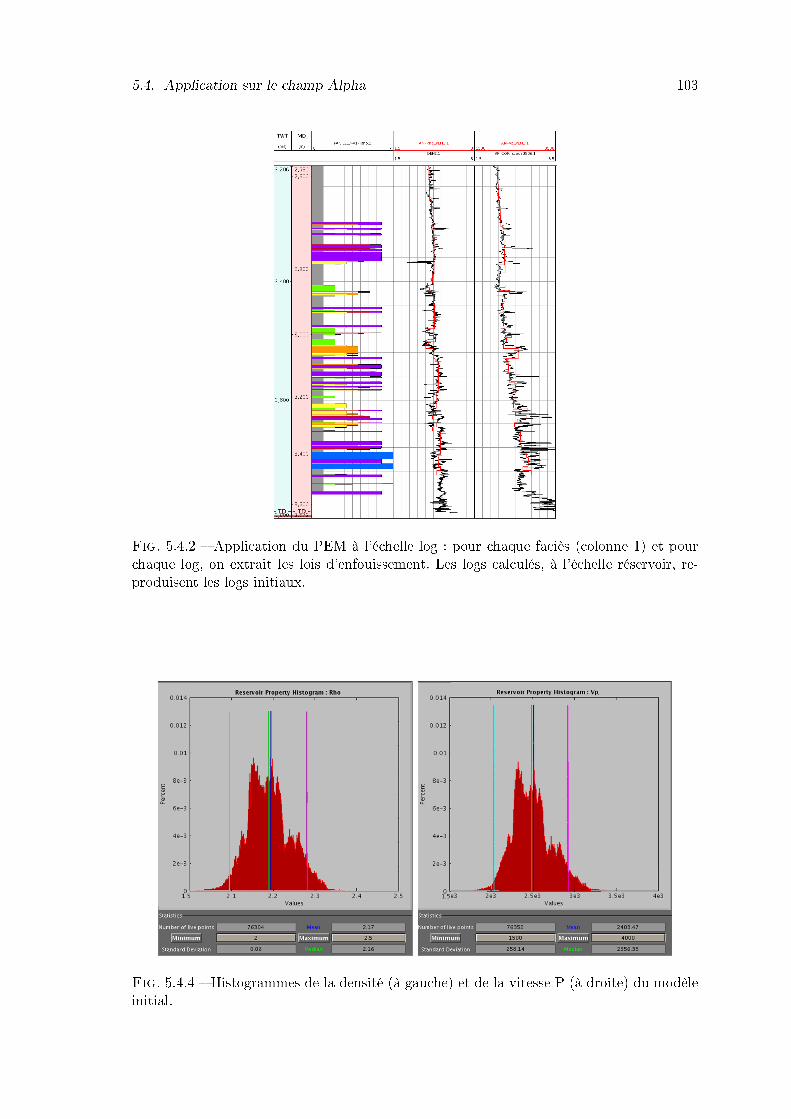
5.4. Application sur le champ Alpha 103
Fig. 5.4.2 � Application du PEM à l'échelle log : pour chaque faciès (colonne 1) et pourchaque log, on extrait les lois d'enfouissement. Les logs calculés, à l'échelle réservoir, re-produisent les logs initiaux.
Fig. 5.4.4 � Histogrammes de la densité (à gauche) et de la vitesse P (à droite) du modèleinitial.

104 Chapitre 5. Inversion par déformation graduelle
5.4.2 Le modèle réelAu chapitre 4, une inversion géostatistique a été réalisée sur le champ Alpha, nous
donnant des impédances avec une résolution verticale très �ne. Ces résultats d'impédancessont upscalés dans la grille réservoir (upscaling) et nous servirons de solution à ce test devalidation de l'inversion par déformations graduelles. Comme l'inversion doit être réaliséeen vitesse P et densité, l'impédance est décomposée en une vitesse P réelle et une densitéréelle par la loi de Gardner et al. 1974 pour des lithologies sables et argiles.
Lithologie d f Intervalle Vp (km/s)Shale 1,75 0,265 1,5-5,0
Sandstone 1,66 0,261 1,5-6,0Limestone 1,50 0,225 3,5-6,4Dolomite 1,74 0,252 4,5-7,1Anhydrite 2,19 0,160 4,6-7,4
Tab. 5.2 � Relations V p−ρ de Gardner par lithologies pour l'équation ρ = dV fp . Les unités
sont km/s et g/cm3
Les propriétés obtenues sont montrés en �gure 5.4.5 et leurs histogrammes sur la �gure5.4.6. À partir de ces propriétés "réelles", nous simulons le volume sismique qui servira decontrainte pour le processus d'inversion.
Fig. 5.4.5 � Densité (à gauche) et vitesse P (à droite) réelles sur la couche 51 du modèleréservoir.
5.4.3 Paramètrisation de l'inversion par déformations graduellesL'anamorphose
Les statistiques des propriétés des modèles initiaux, �naux et des données de puitsmontrent des distributions non-gaussiennes. Or, les déformations graduelles ne s'appliquentque pour des propriétés gaussiennes. Il est donc nécessaire dans le processus d'inversion depasser dans le domaine gaussien par une anamorphose.
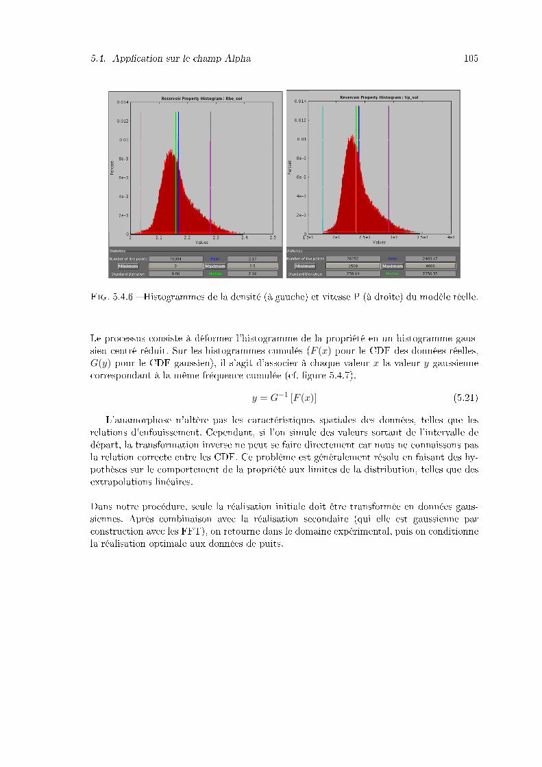
5.4. Application sur le champ Alpha 105
Fig. 5.4.6 � Histogrammes de la densité (à gauche) et vitesse P (à droite) du modèle réelle.
Le processus consiste à déformer l'histogramme de la propriété en un histogramme gaus-sien centré réduit. Sur les histogrammes cumulés (F (x) pour le CDF des données réelles,G(y) pour le CDF gaussien), il s'agit d'associer à chaque valeur x la valeur y gaussiennecorrespondant à la même fréquence cumulée (cf. �gure 5.4.7).
y = G−1 [F (x)] (5.21)L'anamorphose n'altère pas les caractéristiques spatiales des données, telles que les
relations d'enfouissement. Cependant, si l'on simule des valeurs sortant de l'intervalle dedépart, la transformation inverse ne peut se faire directement car nous ne connaissons pasla relation correcte entre les CDF. Ce problème est généralement résolu en faisant des hy-pothèses sur le comportement de la propriété aux limites de la distribution, telles que desextrapolations linéaires.Dans notre procédure, seule la réalisation initiale doit être transformée en données gaus-siennes. Après combinaison avec la réalisation secondaire (qui elle est gaussienne parconstruction avec les FFT), on retourne dans le domaine expérimental, puis on conditionnela réalisation optimale aux données de puits.
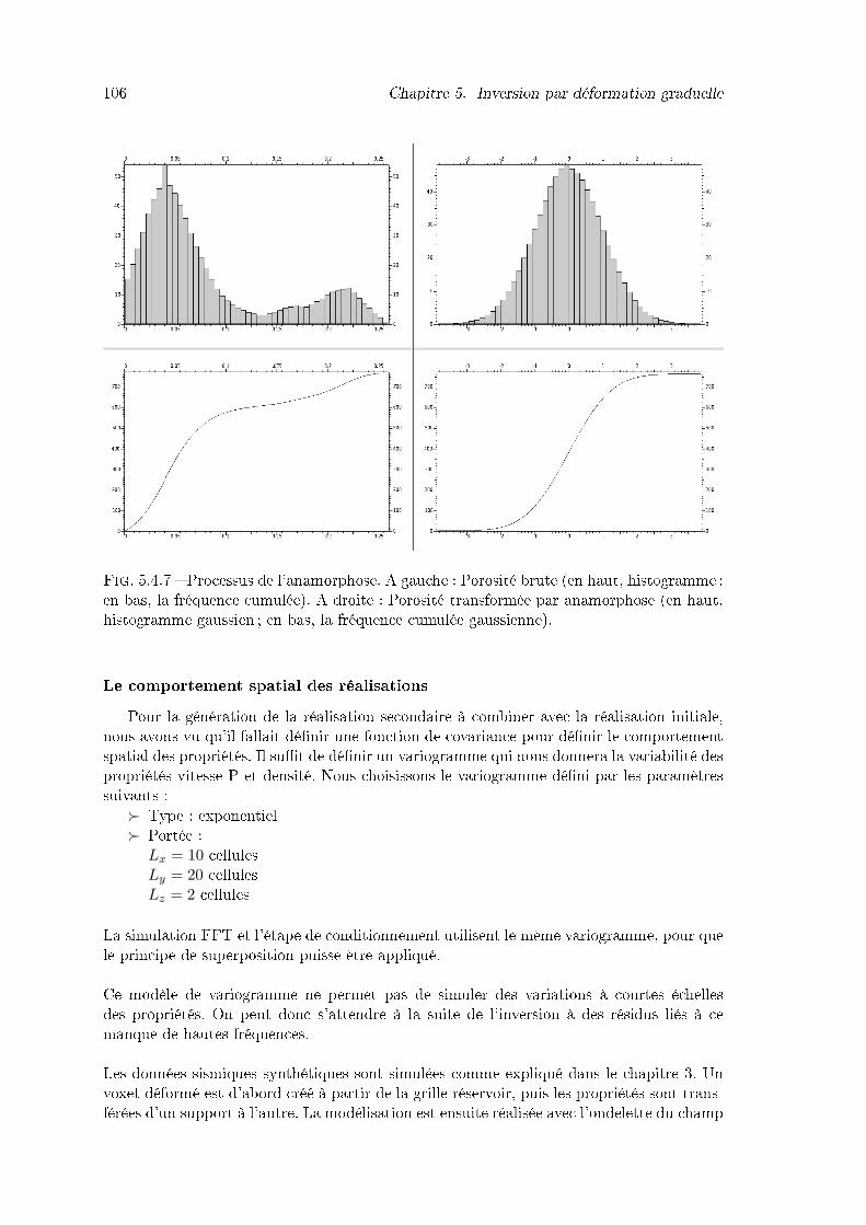
106 Chapitre 5. Inversion par déformation graduelle
Fig. 5.4.7 � Processus de l'anamorphose. A gauche : Porosité brute (en haut, histogramme ;en bas, la fréquence cumulée). A droite : Porosité transformée par anamorphose (en haut,histogramme gaussien ; en bas, la fréquence cumulée gaussienne).
Le comportement spatial des réalisationsPour la génération de la réalisation secondaire à combiner avec la réalisation initiale,
nous avons vu qu'il fallait dé�nir une fonction de covariance pour dé�nir le comportementspatial des propriétés. Il su�t de dé�nir un variogramme qui nous donnera la variabilité despropriétés vitesse P et densité. Nous choisissons le variogramme dé�ni par les paramètressuivants :
� Type : exponentiel� Portée :Lx = 10 cellulesLy = 20 cellulesLz = 2 cellules
La simulation FFT et l'étape de conditionnement utilisent le même variogramme, pour quele principe de superposition puisse être appliqué.Ce modèle de variogramme ne permet pas de simuler des variations à courtes échellesdes propriétés. On peut donc s'attendre à la suite de l'inversion à des résidus liés à cemanque de hautes fréquences.Les données sismiques synthétiques sont simulées comme expliqué dans le chapitre 3. Unvoxet déformé est d'abord créé à partir de la grille réservoir, puis les propriétés sont trans-férées d'un support à l'autre. La modélisation est ensuite réalisée avec l'ondelette du champ
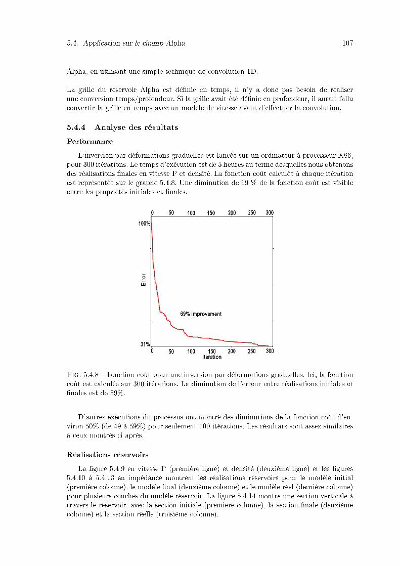
5.4. Application sur le champ Alpha 107
Alpha, en utilisant une simple technique de convolution 1D.La grille du réservoir Alpha est dé�nie en temps, il n'y a donc pas besoin de réaliserune conversion temps/profondeur. Si la grille avait été dé�nie en profondeur, il aurait falluconvertir la grille en temps avec un modèle de vitesse avant d'e�ectuer la convolution.
5.4.4 Analyse des résultatsPerformance
L'inversion par déformations graduelles est lancée sur un ordinateur à processeur X86,pour 300 itérations. Le temps d'exécution est de 5 heures au terme desquelles nous obtenonsdes réalisations �nales en vitesse P et densité. La fonction coût calculée à chaque itérationest représentée sur le graphe 5.4.8. Une diminution de 69 % de la fonction coût est visibleentre les propriétés initiales et �nales.
Fig. 5.4.8 � Fonction coût pour une inversion par déformations graduelles. Ici, la fonctioncoût est calculée sur 300 itérations. La diminution de l'erreur entre réalisations initiales et�nales est de 69%.
D'autres exécutions du processus ont montré des diminutions de la fonction coût d'en-viron 50% (de 49 à 59%) pour seulement 100 itérations. Les résultats sont assez similairesà ceux montrés ci-après.
Réalisations réservoirsLa �gure 5.4.9 en vitesse P (première ligne) et densité (deuxième ligne) et les �gures
5.4.10 à 5.4.13 en impédance montrent les réalisations réservoirs pour le modèle initial(première colonne), le modèle �nal (deuxième colonne) et le modèle réel (dernière colonne)pour plusieurs couches du modèle réservoir. La �gure 5.4.14 montre une section verticale àtravers le réservoir, avec la section initiale (première colonne), la section �nale (deuxièmecolonne) et la section réelle (troisième colonne).
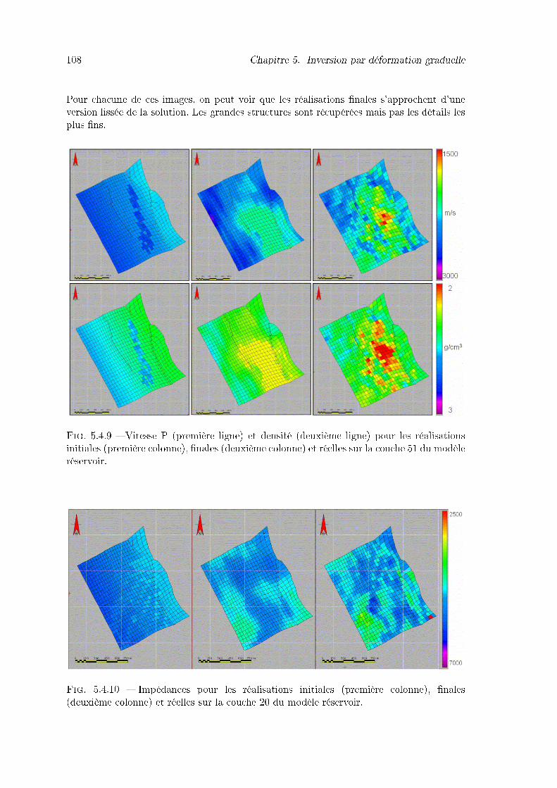
108 Chapitre 5. Inversion par déformation graduelle
Pour chacune de ces images, on peut voir que les réalisations �nales s'approchent d'uneversion lissée de la solution. Les grandes structures sont récupérées mais pas les détails lesplus �ns.
Fig. 5.4.9 � Vitesse P (première ligne) et densité (deuxième ligne) pour les réalisationsinitiales (première colonne), �nales (deuxième colonne) et réelles sur la couche 51 du modèleréservoir.
Fig. 5.4.10 � Impédances pour les réalisations initiales (première colonne), �nales(deuxième colonne) et réelles sur la couche 20 du modèle réservoir.

5.4. Application sur le champ Alpha 109
Fig. 5.4.11 � Impédances pour les réalisations initiales (première colonne), �nales(deuxième colonne) et réelles sur la couche 40 du modèle réservoir.
Fig. 5.4.12 � Impédances pour les réalisations initiales (première colonne), �nales(deuxième colonne) et réelles sur la couche 50 du modèle réservoir.
Fig. 5.4.13 � Impédances pour les réalisations initiales (première colonne), �nales(deuxième colonne) et réelles sur la couche 80 du modèle réservoir.
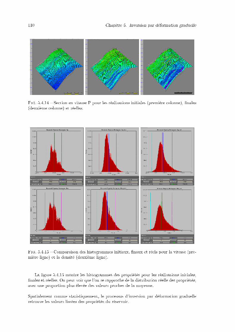
110 Chapitre 5. Inversion par déformation graduelle
Fig. 5.4.14 � Section en vitesse P pour les réalisations initiales (première colonne), �nales(deuxième colonne) et réelles.
Fig. 5.4.15 � Comparaison des histogrammes initiaux, �naux et réels pour la vitesse (pre-mière ligne) et la densité (deuxième ligne).
La �gure 5.4.15 montre les histogrammes des propriétés pour les réalisations initiales,�nales et réelles. On peut voir que l'on se rapproche de la distribution réelle des propriétés,avec une proportion plus élevée des valeurs proches de la moyenne.Spatialement comme statistiquement, le processus d'inversion par déformation graduelleretrouve les valeurs lissées des propriétés du réservoir.
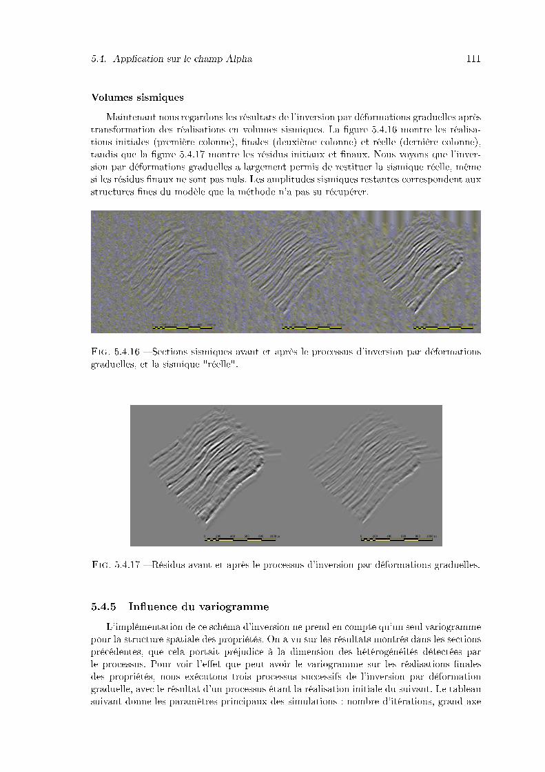
5.4. Application sur le champ Alpha 111
Volumes sismiquesMaintenant nous regardons les résultats de l'inversion par déformations graduelles après
transformation des réalisations en volumes sismiques. La �gure 5.4.16 montre les réalisa-tions initiales (première colonne), �nales (deuxième colonne) et réelle (dernière colonne),tandis que la �gure 5.4.17 montre les résidus initiaux et �naux. Nous voyons que l'inver-sion par déformations graduelles a largement permis de restituer la sismique réelle, mêmesi les résidus �naux ne sont pas nuls. Les amplitudes sismiques restantes correspondent auxstructures �nes du modèle que la méthode n'a pas su récupérer.
Fig. 5.4.16 � Sections sismiques avant et après le processus d'inversion par déformationsgraduelles, et la sismique "réelle".
Fig. 5.4.17 � Résidus avant et après le processus d'inversion par déformations graduelles.
5.4.5 In�uence du variogrammeL'implémentation de ce schéma d'inversion ne prend en compte qu'un seul variogramme
pour la structure spatiale des propriétés. On a vu sur les résultats montrés dans les sectionsprécédentes, que cela portait préjudice à la dimension des hétérogénéités détectées parle processus. Pour voir l'e�et que peut avoir le variogramme sur les réalisations �nalesdes propriétés, nous exécutons trois processus successifs de l'inversion par déformationgraduelle, avec le résultat d'un processus étant la réalisation initiale du suivant. Le tableausuivant donne les paramètres principaux des simulations : nombre d'itérations, grand axe
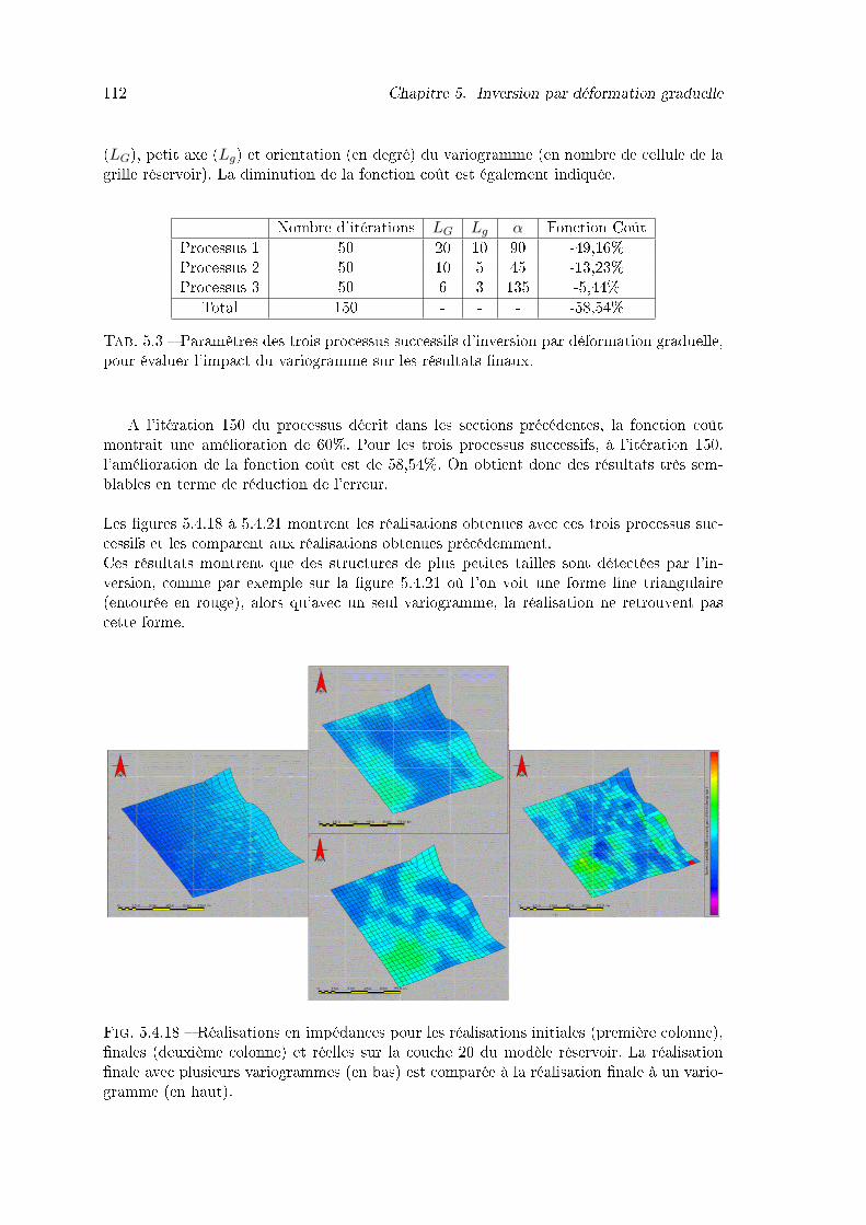
112 Chapitre 5. Inversion par déformation graduelle
(LG), petit axe (Lg) et orientation (en degré) du variogramme (en nombre de cellule de lagrille réservoir). La diminution de la fonction coût est également indiquée.
Nombre d'itérations LG Lg α Fonction CoûtProcessus 1 50 20 10 90 -49,16%Processus 2 50 10 5 45 -13,23%Processus 3 50 6 3 135 -5,44%
Total 150 - - - -58,54%Tab. 5.3 � Paramètres des trois processus successifs d'inversion par déformation graduelle,pour évaluer l'impact du variogramme sur les résultats �naux.
A l'itération 150 du processus décrit dans les sections précédentes, la fonction coûtmontrait une amélioration de 60%. Pour les trois processus successifs, à l'itération 150,l'amélioration de la fonction coût est de 58,54%. On obtient donc des résultats très sem-blables en terme de réduction de l'erreur.Les �gures 5.4.18 à 5.4.21 montrent les réalisations obtenues avec ces trois processus suc-cessifs et les comparent aux réalisations obtenues précédemment.Ces résultats montrent que des structures de plus petites tailles sont détectées par l'in-version, comme par exemple sur la �gure 5.4.21 où l'on voit une forme �ne triangulaire(entourée en rouge), alors qu'avec un seul variogramme, la réalisation ne retrouvent pascette forme.
Fig. 5.4.18 � Réalisations en impédances pour les réalisations initiales (première colonne),�nales (deuxième colonne) et réelles sur la couche 20 du modèle réservoir. La réalisation�nale avec plusieurs variogrammes (en bas) est comparée à la réalisation �nale à un vario-gramme (en haut).
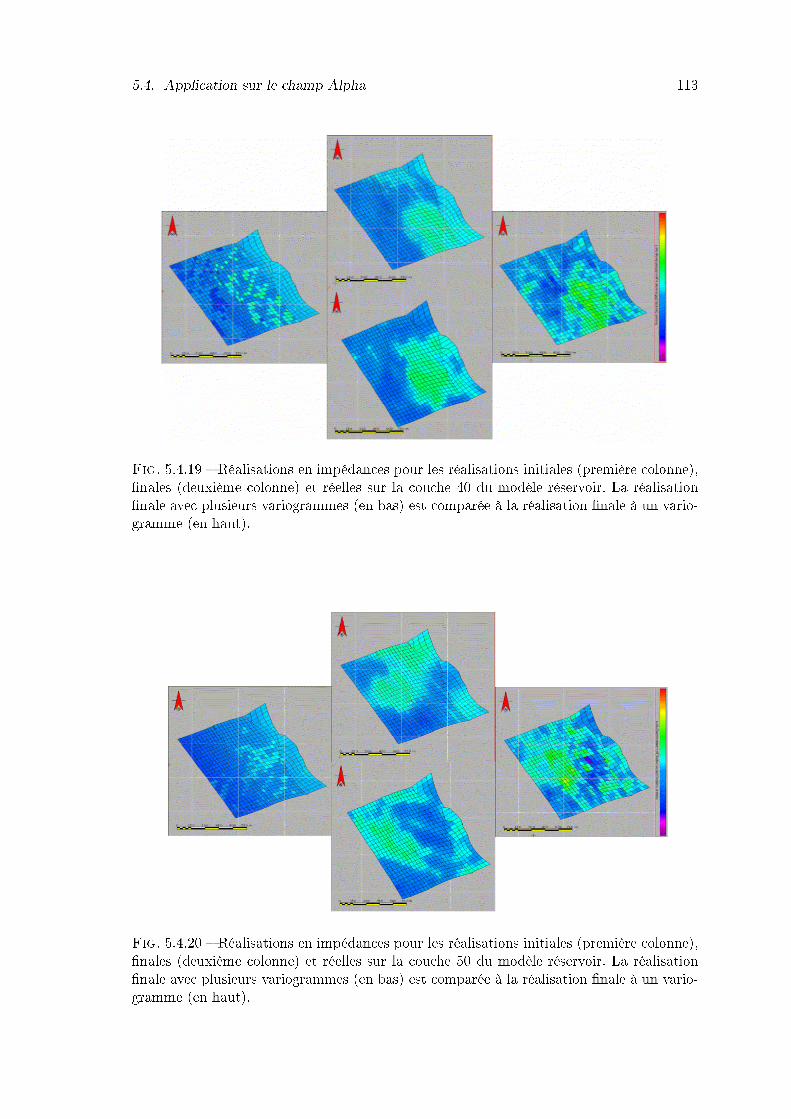
5.4. Application sur le champ Alpha 113
Fig. 5.4.19 � Réalisations en impédances pour les réalisations initiales (première colonne),�nales (deuxième colonne) et réelles sur la couche 40 du modèle réservoir. La réalisation�nale avec plusieurs variogrammes (en bas) est comparée à la réalisation �nale à un vario-gramme (en haut).
Fig. 5.4.20 � Réalisations en impédances pour les réalisations initiales (première colonne),�nales (deuxième colonne) et réelles sur la couche 50 du modèle réservoir. La réalisation�nale avec plusieurs variogrammes (en bas) est comparée à la réalisation �nale à un vario-gramme (en haut).
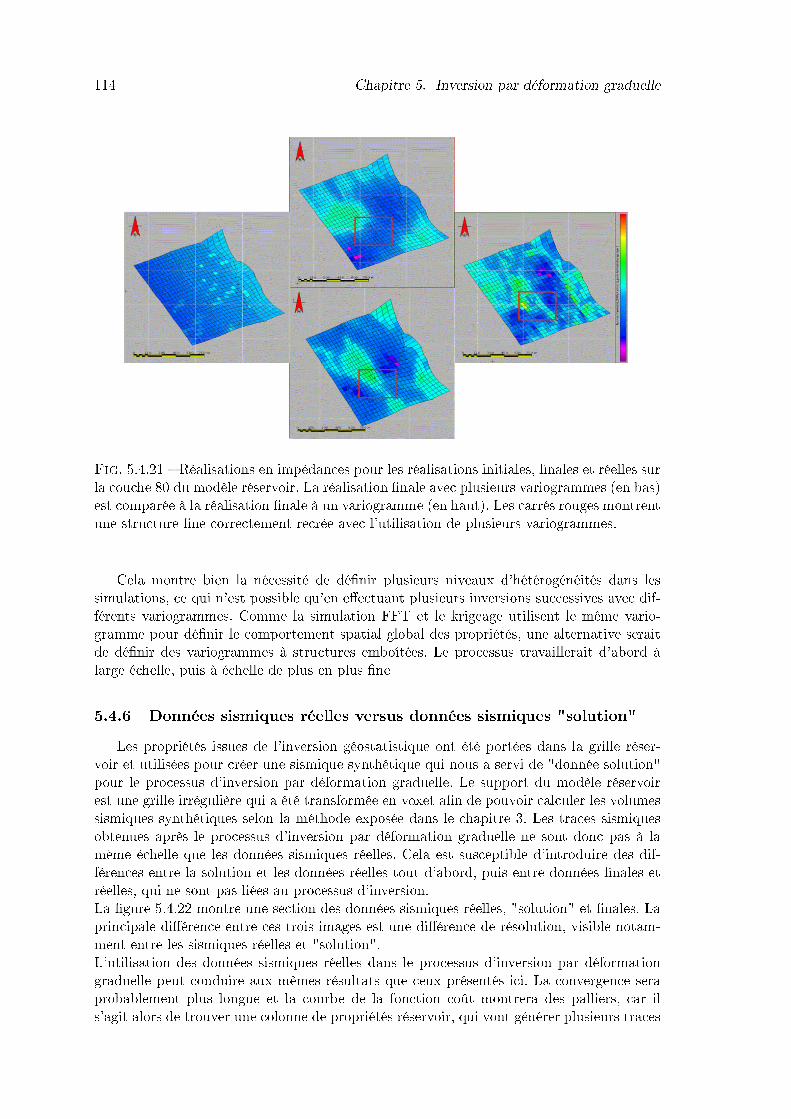
114 Chapitre 5. Inversion par déformation graduelle
Fig. 5.4.21 � Réalisations en impédances pour les réalisations initiales, �nales et réelles surla couche 80 du modèle réservoir. La réalisation �nale avec plusieurs variogrammes (en bas)est comparée à la réalisation �nale à un variogramme (en haut). Les carrés rouges montrentune structure �ne correctement recrée avec l'utilisation de plusieurs variogrammes.
Cela montre bien la nécessité de dé�nir plusieurs niveaux d'hétérogénéités dans lessimulations, ce qui n'est possible qu'en e�ectuant plusieurs inversions successives avec dif-férents variogrammes. Comme la simulation FFT et le krigeage utilisent le même vario-gramme pour dé�nir le comportement spatial global des propriétés, une alternative seraitde dé�nir des variogrammes à structures emboîtées. Le processus travaillerait d'abord àlarge échelle, puis à échelle de plus en plus �ne
5.4.6 Données sismiques réelles versus données sismiques "solution"Les propriétés issues de l'inversion géostatistique ont été portées dans la grille réser-
voir et utilisées pour créer une sismique synthétique qui nous a servi de "donnée solution"pour le processus d'inversion par déformation graduelle. Le support du modèle réservoirest une grille irrégulière qui a été transformée en voxet a�n de pouvoir calculer les volumessismiques synthétiques selon la méthode exposée dans le chapitre 3. Les traces sismiquesobtenues après le processus d'inversion par déformation graduelle ne sont donc pas à lamême échelle que les données sismiques réelles. Cela est susceptible d'introduire des dif-férences entre la solution et les données réelles tout d'abord, puis entre données �nales etréelles, qui ne sont pas liées au processus d'inversion.La �gure 5.4.22 montre une section des données sismiques réelles, "solution" et �nales. Laprincipale di�érence entre ces trois images est une di�érence de résolution, visible notam-ment entre les sismiques réelles et "solution".L'utilisation des données sismiques réelles dans le processus d'inversion par déformationgraduelle peut conduire aux mêmes résultats que ceux présentés ici. La convergence seraprobablement plus longue et la courbe de la fonction coût montrera des palliers, car ils'agit alors de trouver une colonne de propriétés réservoir, qui vont générer plusieurs traces
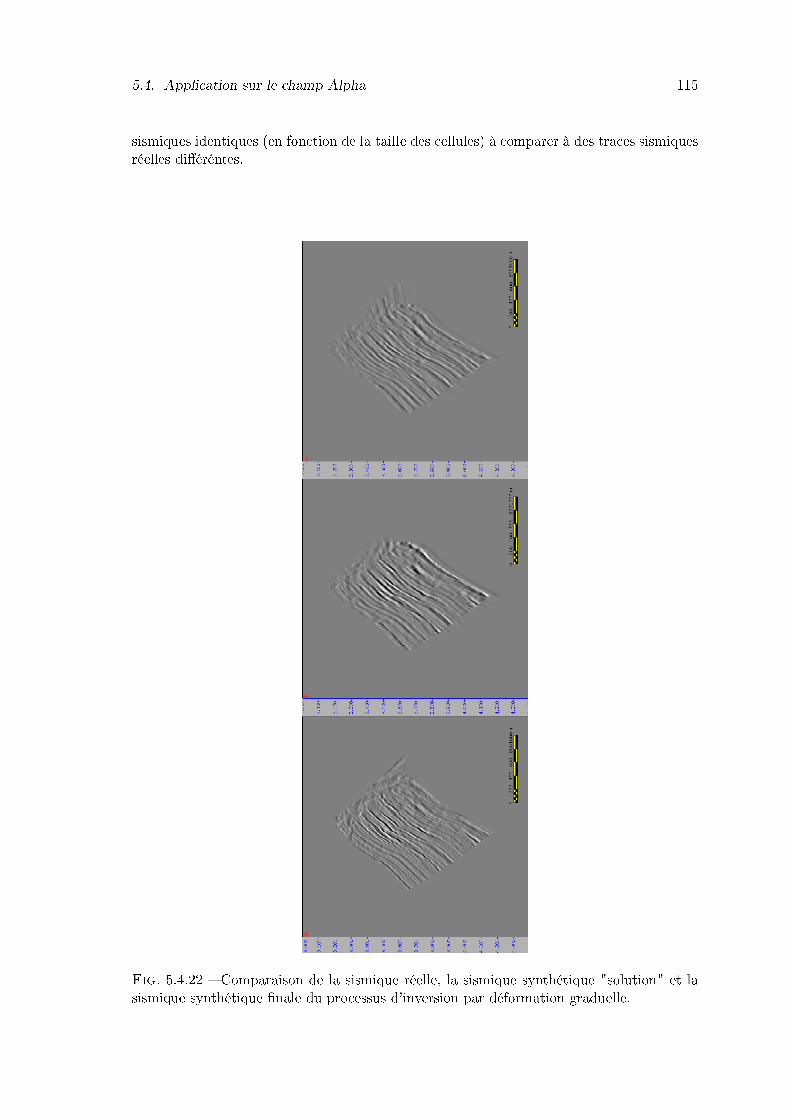
5.4. Application sur le champ Alpha 115
sismiques identiques (en fonction de la taille des cellules) à comparer à des traces sismiquesréelles di�éréntes.
Fig. 5.4.22 � Comparaison de la sismique réelle, la sismique synthétique "solution" et lasismique synthétique �nale du processus d'inversion par déformation graduelle.

116 Chapitre 5. Inversion par déformation graduelle
5.5 Conclusions et perspectivesLe processus d'inversion proposée est une nouvelle méthodologie basée sur une tech-
nique géostatistique, les déformations graduelles, pour simuler des réalisations de propriétésréservoirs cohérentes avec les données sismiques. Les réalisations des propriétés vont êtredéformées progressivement, en améliorant la cohérence avec les données sismiques. Ce pro-cessus fonctionne directement à l'échelle réservoir, tout en faisant la comparaison de laréalisation avec les données réelles dans le domaine sismique. Pour cela, la fonction coûtque l'on cherche à minimiser est basée sur les volumes sismiques réels et synthétiques.Les réalisations sont conditionnées par les données de puits, ce qui introduit une contrainted'ordre géologique. L'implémentation testée ici récupère, soit des impédances, soit des vi-tesses et densités. Cette méthodologie est particulièrement intéressante dans le sens oùelle permet de s'a�ranchir des problèmes liés aux changements d'échelle entre les di�érentssupports.L'implémentation actuelle montre toutefois quelques faiblesses. Les réalisations �nales nerécupèrent pas la partie "haute fréquence" des propriétés. Un premier pas dans l'optimisa-tion de ce processus sera de considérer non pas une, mais plusieurs longueurs de corrélationpour le variogramme de la réalisation secondaire, en allant des larges structures vers les plus�nes par une stratégie emboîtée. Ceci permettra d'introduire plusieurs niveaux d'hétéro-généité dans les simulations. Pour cette première approche d'inversion sismique à l'échelleréservoir, nous avons utilisé la formule de base des déformations graduelles, avec une re-cherche directe pour le paramètre t comme optimisation. L'intégration de la formulationdes déformations graduelles de Hu and Ravalec-Dupin 2004, permet d'associer à la réali-sation initiale, non pas une, mais plusieurs réalisations secondaires, avec des coe�cients trecherchés par une optimisation par gradient. Ceci permettrait d'accélérer la convergencedu processus pour trouver une réalisation réservoir optimale.En�n, en introduisant un modèle pétroélastique, on pourrait dériver directement de cetteinversion des propriétés pétrophysiques dans le réservoir, par exemple les porosités ou lessaturations.

Chapitre 6
Petrophysical inversion by neuralsupervised classi�cation
6.1 IntroductionThe goal of seismic reservoir characterization is to derive reservoir properties from 3D
seismic data with constraints by well logs and a priori geological knowledge. The most im-portant objective is to �nd a relationship between seismic traces and reservoir properties.Three approaches can be considered.In the �rst one, those relationships are derived through the use of geostatistics, neuralnetworks, or multi-linear regression. For example, Fournier and Derain 1992 and deGrootet al. 1993 propose to extract these relationships through statistical calibration of seismicattributes and reservoir parameters at well location. Chandra et al. 2003 use neural net-works to perform a non-supervised classi�cation of seismic data. A seismic facies map iscreated using unsupervised neural networks, and then the porosity trends by facies are ap-plied on the map to derive a porosity volume. Their results clearly show the e�ectiveness ofneural network to identify the stratigraphic features, whereas conventional analysis wouldhave given less satisfactory results. The use of Neural Networks to link seismic parameterswith well information and predict reservoir properties between wells has been successful inseveral instances. But in most cases, the reservoir parameters are the results of a patternrecognition based on seismic trace shapes. These approaches do not rely on petrophysicsto derive the reservoir properties.The second approach performs the inversion of the available data and tries to derive thereservoir properties with calibrated relationships on the seismic attributes, such as Coleouet al. 2006 or such as the work shown in section 4.4 from chapter 4.The third approach uses seismic modeling to visualize the seismic responses due to re-servoir property changes. Julien et al. 2002 have created an application called "MassiveModeling", which creates a large amount of models with a realistic range of structural andpetrophysical variations in the reservoir.We propose a methodology in between the �rst and the third approach.
Our methodology associates a 1D column of petrophysical properties to each seismictrace. To do so, we have to extend the well database, by creating as many pseudo-wellsas needed. In Julien et al. 2002 or Balz et al. 1999, the reservoir parameter variations aredetermined by the user. We propose an improved Massive Modeling scheme to generateall possible 1D models through geostatistical simulations from the wells. Then, we have todetermine which pseudo-log will explain a given seismic trace.One of the best ways to perform this is to learn the seismic response of each pseudo-log,then to predict which model will explain the trace. This is the purpose of neural networks.
117
118 Chapitre 6. Petrophysical inversion by neural supervised classi�cation
In unsupervised neural network, seismic data are classi�ed without a priori information.The results respect logical or mathematical criteria that cannot be evaluated in terms ofpetrophysical properties. In supervised neural nets, the classi�cation is constrained by theseismic response of a priori models. This approach is limited by the amount of data avai-lable.We use the advantages of both neural network approaches (unsupervised and supervisedneural nets) : the logical classi�cation of data in the unsupervised classi�cation, and theconstraints from known relationships in the supervised classi�cation. We use a non super-vised neural network that we apply �rstly on a training set, and then we impose the outputneurons on the actual data. The originality of our methodology lies in the generation ofthe training set (Massive Modeling and geostatistical simulation) and the petrophysicaldiscrimination analysis.The methodology is tested on two di�erent datasets : a clastic case (Beta �eld) and acarbonate case (Gamma �eld).
6.2 The methodologyWe present a new methodology to predict reservoir properties. We create a training set
based on well log data and use it to classify a seismic interval between two horizons in a3D volume, according to the shape of the wiggle traces. To generate the training set, weuse the operating principles of Massive Modeling and geostatistical simulation to derive allpossible scenarii, regarding structural events and petrophysical properties, in the reservoirinterval. Synthetic traces corresponding to these models are computed using a 1D convo-lution. The resulting synthetic traces within the interval are analyzed by neural networks,which generate a series of model traces that best represents the diversity of synthetic data.The resulting set of model traces is applied on actual seismic traces to �nd similar relation-ships between reservoir parameters and seismic response. Finally the results are analyzedin terms of petrophysical discrimination. The classi�cation is based on Kohonen Self Or-ganizing Maps.
The work�ow for the global methodology is illustrated on �gure 6.2.1 and consists inthe following steps :
1. Well log data preparation.� Well log blocking.� Optimization of blocked well logs.� Massive Modeling data generation.
2. Neural network training.� Network learning phase on the training dataset� Validation of petrophysical meaning of the classi�cation
3. Neural network application.� Network validation phase on the test dataset.� Computation of petrophysical property volumes.
The purpose of the well log preparation step is to decrease the number of parametersone will have to handle, and to generate all possible 1D petrophysical models. For eachwell, the logs are blocked, then optimized in regards to the seismic trace at the same lo-cation. Once available, these "best" logs are input to the Massive Modeling scheme. New
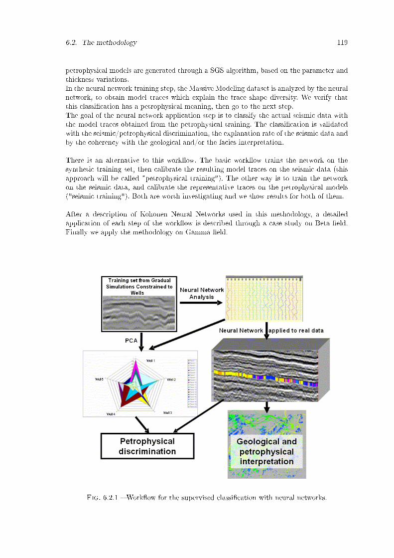
6.2. The methodology 119
petrophysical models are generated through a SGS algorithm, based on the parameter andthickness variations.In the neural network training step, the Massive Modeling dataset is analyzed by the neuralnetwork, to obtain model traces which explain the trace shape diversity. We verify thatthis classi�cation has a petrophysical meaning, then go to the next step.The goal of the neural network application step is to classify the actual seismic data withthe model traces obtained from the petrophysical training. The classi�cation is validatedwith the seismic/petrophysical discrimination, the explanation rate of the seismic data andby the coherency with the geological and/or the facies interpretation.There is an alternative to this work�ow. The basic work�ow trains the network on thesynthetic training set, then calibrate the resulting model traces on the seismic data (thisapproach will be called "petrophysical training"). The other way is to train the networkon the seismic data, and calibrate the representative traces on the petrophysical models("seismic training"). Both are worth investigating and we show results for both of them.After a description of Kohonen Neural Networks used in this methodology, a detailedapplication of each step of the work�ow is described through a case study on Beta �eld.Finally we apply the methodology on Gamma �eld.
Fig. 6.2.1 � Work�ow for the supervised classi�cation with neural networks.

120 Chapitre 6. Petrophysical inversion by neural supervised classi�cation
6.3 Neural Networks : Kohonen Self-Organizing MapsNeural networks are methods based on brain function and on the concept of neuron.
They are known for their versatility and their ability to solve complex, nonlinear problemson noisy data. The idea is to replicate the brain mechanism of learning, that is, the adap-tation of an individual to a new concept.Neural networks are constituted of several layers of interconnected neurons in input anddata output. Following a learning phase, neurons are linked to the data by minimizing theerror between simulated signal and known signal. Optimization by neural networks requiresno a priori information on input/output relationships, but the quality of optimization hea-vily depends on the learning phase. Indeed, if the signal is complex, the learning phase willhave to be important to stabilize the neural connections to the output data.
Neural Networks are used since the early 1980s in geophysics and since the 1990s inreservoir characterization (Poulton 2002). We want to perform a trace shape classi�ca-tion using a robust pattern-recognition process such as the Kohonen Self Organizing Map(KSOM) method (Kohonen 1990) ; it is well suited to seismic data due to its ability to�lter out noise and identify representative traces in the reservoir intervals.The KSOM is a type of Arti�cial Neural Network that is trained using unsupervised lear-ning. It describes a mapping from a higher dimensional input space to a lower dimensionalmap space (one dimensional in this case). KSOMs are used to study the repartition of datain a N-dimensional space by simply inspecting the data for regularities and characteristics.This kind of networks organizes itself in such a way as to create an ordered description ofthe data.
6.3.0.1 Some generalities on Kohonen Self Organizing MapsKSOMs are mathematical structures that reproduce complex and non linear relation-
ships between input data (the seismic traces) and output data (the neurons representedby model traces) with parameters (weight) which are adjusted during the learning phase,described hereafter.A set of neurons M receives an input data X in a vectorial shape X = (x1, x2, . . . , xN )with weights W = (w1, w2, . . . , wN ). The winning neuron (the neuron which is the closestto the input data) is determined by computing the Euclidian distance for each neuron andby choosing the neuron with the lesser value. Then the winning neuron is updated so as tohave a better match with the input data. The neighbours of this neuron are also updatedin a smaller proportion. The update formula for a neuron with weight vector wi(t) is
wi(t+ 1) = wi(t) + φ(i, t) ∗ α(τ)(Xi(t)− wi(t)), (6.1)Where α(τ) is a monotonically decreasing learning coe�cient and Xi(t) is the input vector.The neighbourhood function φ(i, t) depends on the distance between the winning neuronand neuron i. Regardless of its original value, the neighbourhood function shrinks withtime. At the beginning when the neighbourhood is broad, the self-organizing takes placeon the global scale. This will move each unit in the neighbourhood closer to the inputpattern.As time progresses the learning rate and the neighbourhood size are reduced. When thenumber of iteration is reached, each neuron is independent. If the parameters are well
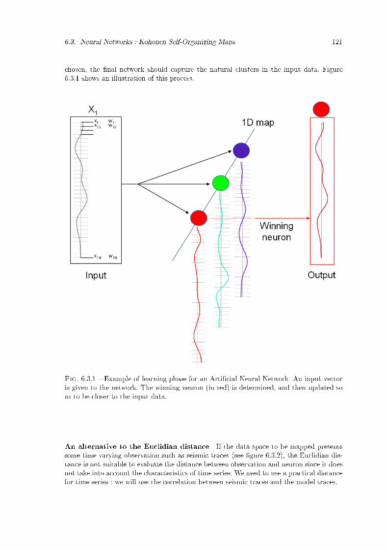
6.3. Neural Networks : Kohonen Self-Organizing Maps 121
chosen, the �nal network should capture the natural clusters in the input data. Figure6.3.1 shows an illustration of this process.
Fig. 6.3.1 � Example of learning phase for an Arti�cial Neural Network. An input vectoris given to the network. The winning neuron (in red) is determined, and then updated soas to be closer to the input data.
An alternative to the Euclidian distance If the data space to be mapped presentssome time varying observation such as seismic traces (see �gure 6.3.2), the Euclidian dis-tance is not suitable to evaluate the distance between observation and neuron since it doesnot take into account the characteristics of time series. We need to use a practical distancefor time series : we will use the correlation between seismic traces and the model traces.
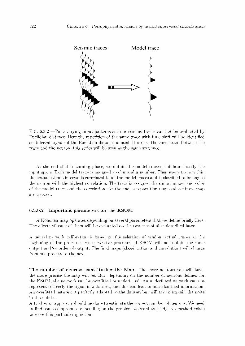
122 Chapitre 6. Petrophysical inversion by neural supervised classi�cation
Fig. 6.3.2 � Time varying input patterns such as seismic traces can not be evaluated byEuclidian distance. Here the repetition of the same trace with time shift will be identi�edas di�erent signals if the Euclidian distance is used. If we use the correlation between thetrace and the neuron, this series will be seen as the same sequence.
At the end of this learning phase, we obtain the model traces that best classify theinput space. Each model trace is assigned a color and a number. Then every trace withinthe actual seismic interval is correlated to all the model traces and is classi�ed to belong tothe neuron with the highest correlation. The trace is assigned the same number and colorof the model trace and the correlation. At the end, a repartition map and a �tness mapare created.
6.3.0.2 Important parameters for the KSOMA Kohonen map operates depending on several parameters that we de�ne brie�y here.
The e�ects of some of them will be evaluated on the two case studies described later.A neural network calibration is based on the selection of random actual traces at thebeginning of the process : two successive processes of KSOM will not obtain the sameoutput and/or order of output. The �nal maps (classi�cation and correlation) will changefrom one process to the next.
The number of neurons constituting the Map The more neurons you will have,the more precise the map will be. But, depending on the number of neurons de�ned forthe KSOM, the network can be over�tted or under�tted. An under�tted network can notrepresent correctly the signal in a dataset, and this can lead to non identi�ed information.An over�tted network is perfectly adapted to the dataset but will try to explain the noisein these data.A trial-error approach should be done to estimate the correct number of neurons. We needto �nd some compromise depending on the problem we want to study. No method existsto solve this particular question.
6.3. Neural Networks : Kohonen Self-Organizing Maps 123
The size of the neighbourhood The neighbourhood radius gives the size of the activeenvironment for a neuron. This means that the neurons inside the radius of the winningneuron will be modi�ed regarding to the learning law. With the number of iteration, thisradius decreases until all neurons are independent.
This parameter is very important since it controls the repartition of the neurons in themap. For example, if we constrain the learning process with a big neighbourhood radius,the algorithm will have some trouble to �nd speci�c zones. Inversely, with a small radius,we will map too many speci�c zones, which have no real signi�cation.
The learning rate (α) The learning rate is the maximum amplitude of the modi�cationsto be applied on each neuron at each step (or iteration) :
α(τ) = α0(1−τ
τ∞) (6.2)
With α0 the learning rate at τ = 0 and τ∞ the number of iteration.This parameter controls the convergence rate. When the value of α is high, the algorithmconverges quickly toward a representation of the data space, but we can have some insta-bilities in the process, leading to the loss of the learning. For example, if α = 1, the outputneuron will be the last observation to be presented, regardless of all observations analyzedbefore that. Generally, this learning rate is quite weak (α = 0.01 typically). This way, themodi�cations on one neuron will be gradual during the learning process.
The number of iteration τ The number of iteration τ has an in�uence on the neigh-bourhood radius and the learning rate. At the beginning of the learning phase, if we havea neighbourhood radius of 2 for example, this means that the winning neuron and the fourneurons around it (two on one side, two on the other side of the map) are updated whenan input trace is presented. Also, the learning rate is strong, so the model traces undergoan important change. At the end of the learning phase, each neuron is independent (onlythe winning neuron is updated) and there is little change on the shape of the trace sincealmost all input data has been presented and the model traces are stable/stationary.

124 Chapitre 6. Petrophysical inversion by neural supervised classi�cation
6.4 Data preparation for the Beta �eldThe methodology is applied on a clastic case : Beta �eld described in chapter 2, with 5
available wells (all slightly deviated). The reservoir is 70ms thick on the seismic data (see�gure 6.4.1). The Beta �eld shows a very high petrophysical variability between wells. Theobjective of this study is to see if geological bodies can be discriminated by the methodology.
Fig. 6.4.1 � A seismic section for the Beta �eld, showing the reservoir of interest delimitedby the green horizons.
6.4.1 Well log preparation6.4.1.1 Well log blocking
The original logs consist in P and S velocities and densities. All logs should be blockedat the stratigraphic scale in order to reduce the number of parameters to handle for theoptimization. This representation maintains the shape of the original log curves, which isessential for the stratigraphic interpretation, while making the optimization task easier.The blocking is done by de�ning major geological markers and by averaging the log samplesbetween two successive markers. The number of de�ned markers is chosen to remove thehigh-frequency information, which is not visible at seismic resolution, but also representglobally the logs on the interval of interest, while retaining the essential petrophysical va-riability for reservoir characterization.The geological interpretation from Beta �eld provides several stratigraphic markers foreach well, but the number di�ers between the wells. Basically, those markers follow thecorrelation sheet shown in �gure 6.4.2.We need to create a few new markers so as to obtain the same number of macro-layersfor each well (here 18 macro-layers were de�ned). An example of results for this blockingstep is shown on well W-Beta3 in �gure 6.4.4, where the synthetic of the blocked logs is
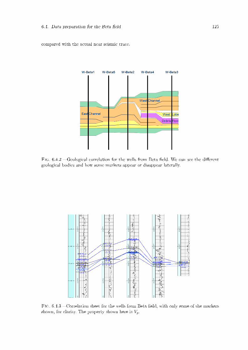
6.4. Data preparation for the Beta �eld 125
compared with the actual near seismic trace.
Fig. 6.4.2 � Geological correlation for the wells from Beta �eld. We can see the di�erentgeological bodies and how some markers appear or disappear laterally.
Fig. 6.4.3 � Correlation sheet for the wells from Beta �eld, with only some of the markersshown, for clarity. The property shown here is Vp.
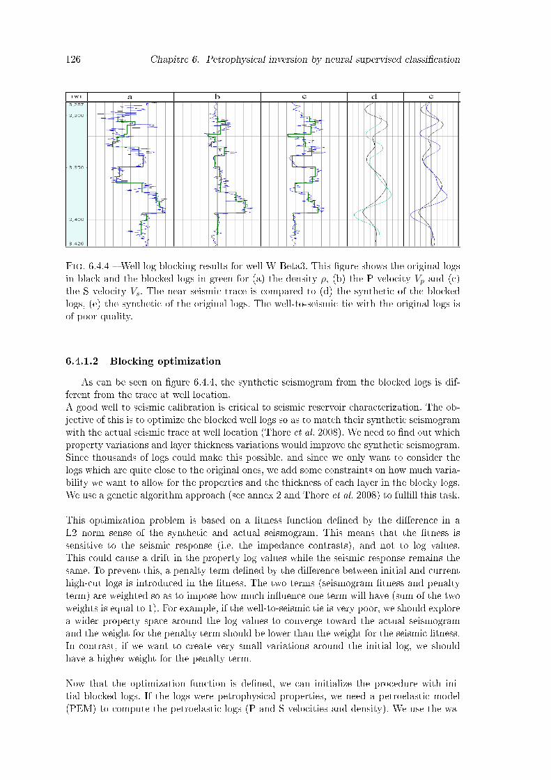
126 Chapitre 6. Petrophysical inversion by neural supervised classi�cation
Fig. 6.4.4 � Well log blocking results for well W-Beta3. This �gure shows the original logsin black and the blocked logs in green for (a) the density ρ, (b) the P velocity Vp and (c)the S velocity Vs. The near seismic trace is compared to (d) the synthetic of the blockedlogs, (e) the synthetic of the original logs. The well-to-seismic tie with the original logs isof poor quality.
6.4.1.2 Blocking optimizationAs can be seen on �gure 6.4.4, the synthetic seismogram from the blocked logs is dif-
ferent from the trace at well location.A good well to seismic calibration is critical to seismic reservoir characterization. The ob-jective of this is to optimize the blocked well logs so as to match their synthetic seismogramwith the actual seismic trace at well location (Thore et al. 2008). We need to �nd out whichproperty variations and layer thickness variations would improve the synthetic seismogram.Since thousands of logs could make this possible, and since we only want to consider thelogs which are quite close to the original ones, we add some constraints on how much varia-bility we want to allow for the properties and the thickness of each layer in the blocky logs.We use a genetic algorithm approach (see annex 2 and Thore et al. 2008) to ful�ll this task.This optimization problem is based on a �tness function de�ned by the di�erence in aL2 norm sense of the synthetic and actual seismogram. This means that the �tness issensitive to the seismic response (i.e. the impedance contrasts), and not to log values.This could cause a drift in the property log values while the seismic response remains thesame. To prevent this, a penalty term de�ned by the di�erence between initial and currenthigh-cut logs is introduced in the �tness. The two terms (seismogram �tness and penaltyterm) are weighted so as to impose how much in�uence one term will have (sum of the twoweights is equal to 1). For example, if the well-to-seismic tie is very poor, we should explorea wider property space around the log values to converge toward the actual seismogramand the weight for the penalty term should be lower than the weight for the seismic �tness.In contrast, if we want to create very small variations around the initial log, we shouldhave a higher weight for the penalty term.Now that the optimization function is de�ned, we can initialize the procedure with ini-tial blocked logs. If the logs were petrophysical properties, we need a petroelastic model(PEM) to compute the petroelastic logs (P and S velocities and density). We use the wa-
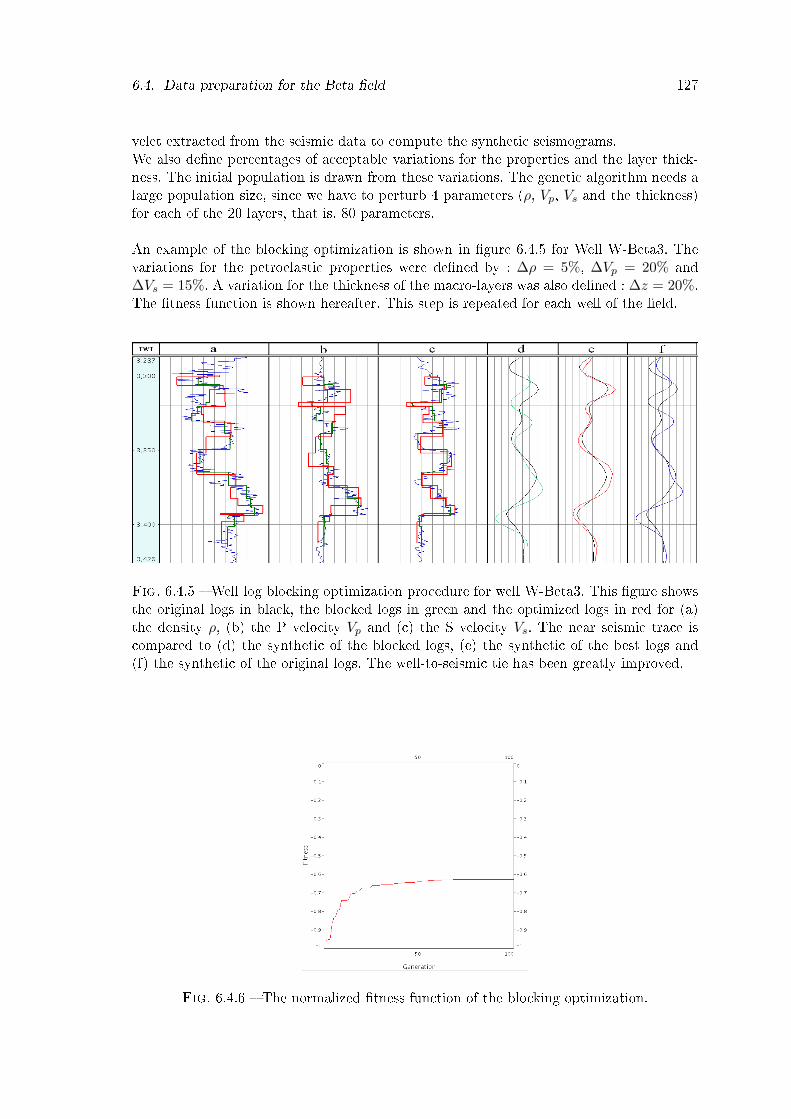
6.4. Data preparation for the Beta �eld 127
velet extracted from the seismic data to compute the synthetic seismograms.We also de�ne percentages of acceptable variations for the properties and the layer thick-ness. The initial population is drawn from these variations. The genetic algorithm needs alarge population size, since we have to perturb 4 parameters (ρ, Vp, Vs and the thickness)for each of the 20 layers, that is, 80 parameters.An example of the blocking optimization is shown in �gure 6.4.5 for Well W-Beta3. Thevariations for the petroelastic properties were de�ned by : ∆ρ = 5%, ∆Vp = 20% and∆Vs = 15%. A variation for the thickness of the macro-layers was also de�ned : ∆z = 20%.The �tness function is shown hereafter. This step is repeated for each well of the �eld.
Fig. 6.4.5 � Well log blocking optimization procedure for well W-Beta3. This �gure showsthe original logs in black, the blocked logs in green and the optimized logs in red for (a)the density ρ, (b) the P velocity Vp and (c) the S velocity Vs. The near seismic trace iscompared to (d) the synthetic of the blocked logs, (e) the synthetic of the best logs and(f) the synthetic of the original logs. The well-to-seismic tie has been greatly improved.
Fig. 6.4.6 � The normalized �tness function of the blocking optimization.

128 Chapitre 6. Petrophysical inversion by neural supervised classi�cation
6.4.1.3 Massive ModelingThe Massive Modeling approach, as described by Julien et al. 2002, works with limited
well knowledge, by simulating virtual wells and their logs, with hypothesis of petroelasticproperty and thickness changes. This method is based on the pseudo-well technique whichis "a method to simulate wells, i.e., 1D stratigraphic pro�les with attached physical proper-ties but without spatial information, using a combination of geological knowledge and MonteCarlo statistics", as stated by deGroot et al. 1996. This approach has a main drawback :the estimation of property variation ranges by expert knowledge is not a trivial task, andthe generation of corresponding models may not be representative enough of all possiblegeological scenarii.We propose an improved Massive Modeling scheme, using geostatistics to derive propertyand thickness variability from available wells, and generate all possible 1D models.This scheme generates new models from the optimized logs (after well log preprocessing)in two main steps :
� Get current layer thickness and property variations of all available wells.� Perform Sequential Gaussian Simulation to create the new models.
Fig. 6.4.7 � At each location U, for each parameter and each layer, the SGS method drawsvalues Y from the CCDF provided by the parameter statistics extracted from the wells.
SGS is the most used algorithm to generate conditional realizations. For details onthe SGS algorithm, one can consult Chiles and Del�ner 1999 and Goovaerts 1997. In thegaussian domain, we draw a continuous line from the conditional cumulative distributionfunction (CCDF) provided by the parameter statistics extracted from the wells, with dif-ferent values for each location of the simulated dataset (see �gure 6.4.7). When we go backto the empirical domain, we obtain the values for each property in one layer. By repeatingthis for each layer of the logs, we obtain a new simulated log for which we compute thesynthetic. Then this new log is considered as a hard data (a constraint) when we proceedto the next location. Figure 6.4.8 shows the properties and synthetics of a small part ofthe Massive Modeling volume. Each 50 traces, an actual well has been placed to constrainthe simulation.
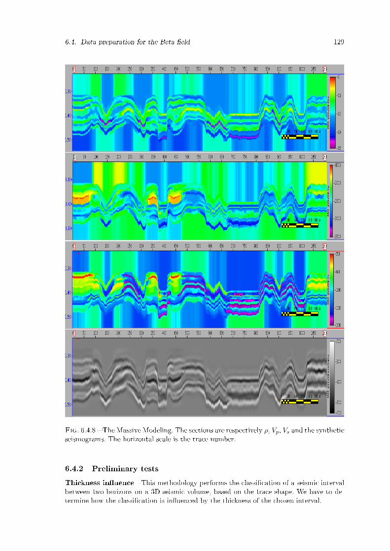
6.4. Data preparation for the Beta �eld 129
Fig. 6.4.8 � The Massive Modeling. The sections are respectively ρ, Vp, Vs and the syntheticseismograms. The horizontal scale is the trace number.
6.4.2 Preliminary testsThickness in�uence This methodology performs the classi�cation of a seismic intervalbetween two horizons on a 3D seismic volume, based on the trace shape. We have to de-termine how the classi�cation is in�uenced by the thickness of the chosen interval.
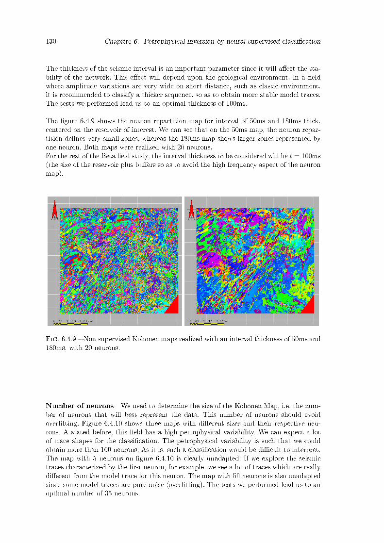
130 Chapitre 6. Petrophysical inversion by neural supervised classi�cation
The thickness of the seismic interval is an important parameter since it will a�ect the sta-bility of the network. This e�ect will depend upon the geological environment. In a �eldwhere amplitude variations are very wide on short distance, such as clastic environment,it is recommended to classify a thicker sequence, so as to obtain more stable model traces.The tests we performed lead us to an optimal thickness of 100ms.The �gure 6.4.9 shows the neuron repartition map for interval of 50ms and 180ms thick,centered on the reservoir of interest. We can see that on the 50ms map, the neuron repar-tition de�nes very small zones, whereas the 180ms map shows larger zones represented byone neuron. Both maps were realized with 20 neurons.For the rest of the Beta �eld study, the interval thickness to be considered will be t = 100ms(the size of the reservoir plus bu�ers so as to avoid the high frequency aspect of the neuronmap).
Fig. 6.4.9 � Non supervised Kohonen maps realized with an interval thickness of 50ms and180ms, with 20 neurons.
Number of neurons We need to determine the size of the Kohonen Map, i.e. the num-ber of neurons that will best represent the data. This number of neurons should avoidover�tting. Figure 6.4.10 shows three maps with di�erent sizes and their respective neu-rons. A stated before, this �eld has a high petrophysical variability. We can expect a lotof trace shapes for the classi�cation. The petrophysical variability is such that we couldobtain more than 100 neurons. As it is, such a classi�cation would be di�cult to interpret.The map with 5 neurons on �gure 6.4.10 is clearly unadapted. If we explore the seismictraces characterized by the �rst neuron, for example, we see a lot of traces which are reallydi�erent from the model trace for this neuron. The map with 50 neurons is also unadaptedsince some model traces are pure noise (over�tting). The tests we performed lead us to anoptimal number of 35 neurons.
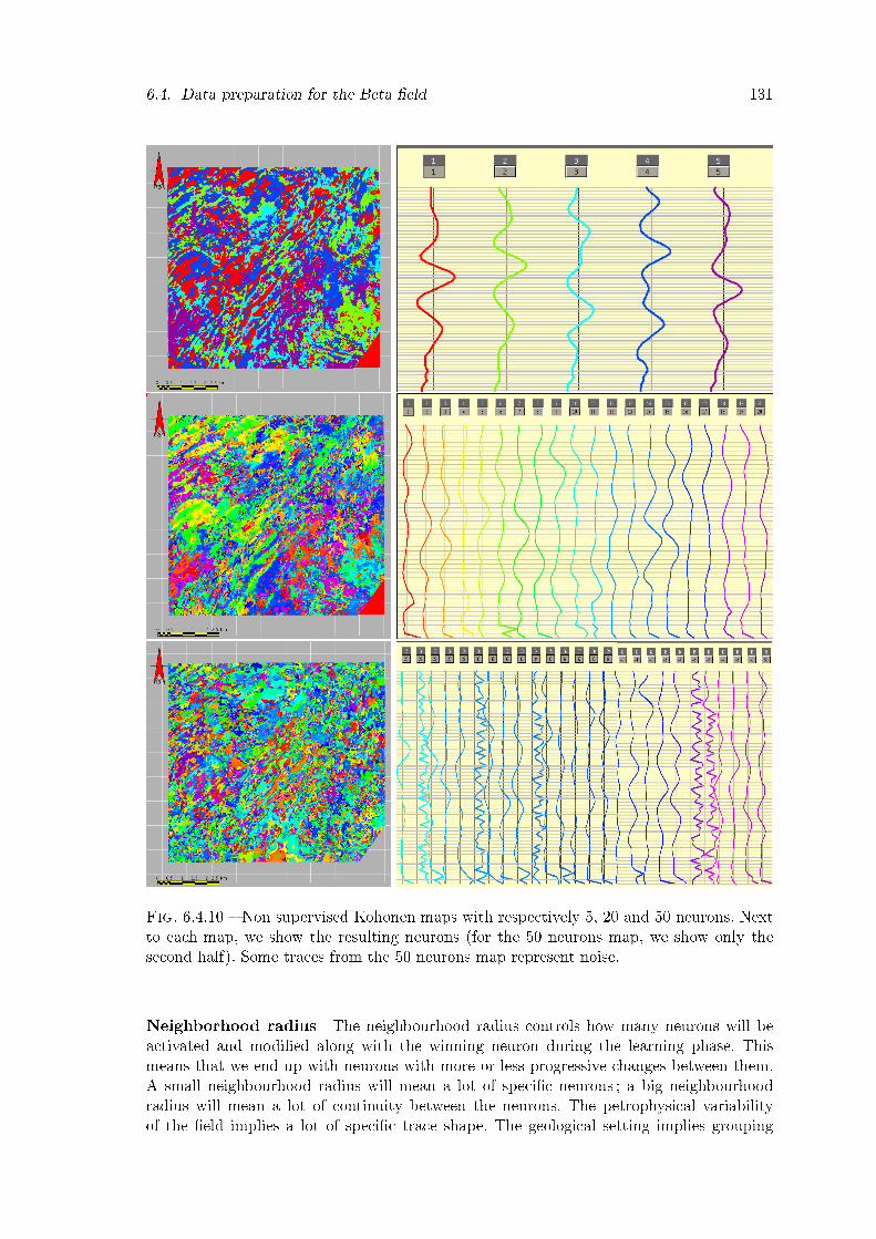
6.4. Data preparation for the Beta �eld 131
Fig. 6.4.10 � Non supervised Kohonen maps with respectively 5, 20 and 50 neurons. Nextto each map, we show the resulting neurons (for the 50 neurons map, we show only thesecond half). Some traces from the 50 neurons map represent noise.
Neighborhood radius The neighbourhood radius controls how many neurons will beactivated and modi�ed along with the winning neuron during the learning phase. Thismeans that we end up with neurons with more or less progressive changes between them.A small neighbourhood radius will mean a lot of speci�c neurons ; a big neighbourhoodradius will mean a lot of continuity between the neurons. The petrophysical variabilityof the �eld implies a lot of speci�c trace shape. The geological setting implies grouping
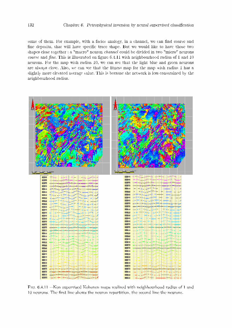
132 Chapitre 6. Petrophysical inversion by neural supervised classi�cation
some of them. For example, with a facies analogy, in a channel, we can �nd coarse and�ne deposits, that will have speci�c trace shape. But we would like to have those twoshapes close together : a "macro" neuron channel could be divided in two "micro" neuronscoarse and �ne. This is illustrated on �gure 6.4.11 with neighbourhood radius of 1 and 10neurons. For the map with radius 10, we can see that the light blue and green neuronsare always close. Also, we can see that the �tness map for the map with radius 1 has aslightly more elevated average value. This is because the network is less constrained by theneighbourhood radius.
Fig. 6.4.11 � Non supervised Kohonen maps realized with neighbourhood radius of 1 and10 neurons. The �rst line shows the neuron repartition, the second line the neurons.
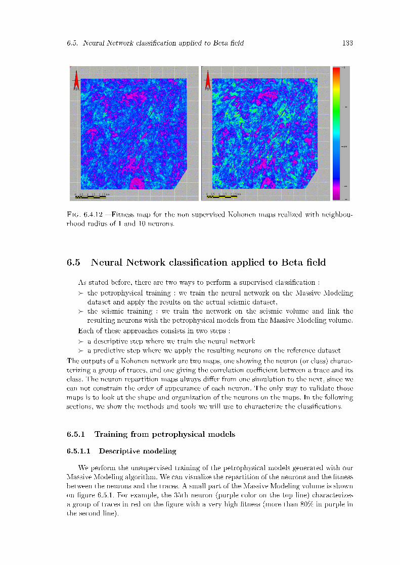
6.5. Neural Network classi�cation applied to Beta �eld 133
Fig. 6.4.12 � Fitness map for the non supervised Kohonen maps realized with neighbou-rhood radius of 1 and 10 neurons.
6.5 Neural Network classi�cation applied to Beta �eld
As stated before, there are two ways to perform a supervised classi�cation :� the petrophysical training : we train the neural network on the Massive Modeling
dataset and apply the results on the actual seismic dataset,� the seismic training : we train the network on the seismic volume and link the
resulting neurons with the petrophysical models from the Massive Modeling volume.Each of these approaches consists in two steps :� a descriptive step where we train the neural network� a predictive step where we apply the resulting neurons on the reference dataset
The outputs of a Kohonen network are two maps, one showing the neuron (or class) charac-terizing a group of traces, and one giving the correlation coe�cient between a trace and itsclass. The neuron repartition maps always di�er from one simulation to the next, since wecan not constrain the order of appearance of each neuron. The only way to validate thosemaps is to look at the shape and organization of the neurons on the maps. In the followingsections, we show the methods and tools we will use to characterize the classi�cations.
6.5.1 Training from petrophysical models6.5.1.1 Descriptive modeling
We perform the unsupervised training of the petrophysical models generated with ourMassive Modeling algorithm. We can visualize the repartition of the neurons and the �tnessbetween the neurons and the traces. A small part of the Massive Modeling volume is shownon �gure 6.5.1. For example, the 35th neuron (purple color on the top line) characterizesa group of traces in red on the �gure with a very high �tness (more than 80% in purple inthe second line).

134 Chapitre 6. Petrophysical inversion by neural supervised classi�cation
Fig. 6.5.1 � A small part of the Massive Modeling volume, with the neuron repartition(top line) and the �tness (bottom line) for each trace.
Visualization of the classi�cation We can easily visualize the result of the classi�ca-tion, by representing each trace with color-coding for the class number and the �tness (see�gure 6.5.2). The background color indicates the class number to which the record belongs,and the saturation of the color indicates the �tness. For example, all red traces belong toclass 1. Dark red means a very high �tness ; light red means a weak �tness. At the top ofthe window, the traces are not sorted and are in the normal order of the seismic block. Atthe bottom of the window, they are sorted by class number and �tness. This display showsthe general organization of the model traces on the dataset.
Fig. 6.5.2 � A small part of the color-coded visualization of the classi�cation. On the top-row, the traces are shown as they are in the dataset. On the bottom-row, the traces areordered by class and �tness. Since we show about 300 traces, once ordered we see only asmall portion of two classes on the bottom row.

6.5. Neural Network classi�cation applied to Beta �eld 135
Classi�cation QC A graph is created using the �tness map from the Kohonen network,representing the percentage of traces with �tness greater than or equal to the �tness abs-cissa. This way we can see if the output neurons from the Kohonen classi�cation are wellsuited with the traces of the dataset.
Fig. 6.5.3 � A graph showing the percentage of model traces exceeding the �tness on theabscissa. For example, 50% of the model traces have a �tness greater than 90%, which isfully satisfactory.
The graph 6.5.3, applied on the Massive Modeling volume, shows that the model tracesexplain the petrophysical models.
Classi�cation analysis The analysis of classi�cation provides a link between the tracecharacteristics determined by the classi�cation and the input parameters of the seismicmodeling.For each class, the algorithm retrieves all traces belonging to the class and with �tness abovethe threshold. It then calculates the average and standard deviation on all these traces foreach input parameter of the model and for each layer. These results are presented in thetable 6.5.4. Such tables enable to follow the behaviour of the petrophysical models in astatistical sense.
Fig. 6.5.4 � A part of the table for the classi�cation analysis. We obtain the parameteraverage and standard deviation for each neuron. Here are shown the thickness, ρ and Vp
for the two �rst layers and the three �rst neurons.
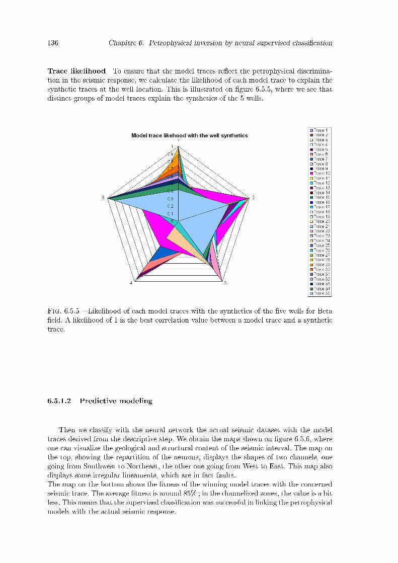
136 Chapitre 6. Petrophysical inversion by neural supervised classi�cation
Trace likelihood To ensure that the model traces re�ect the petrophysical discrimina-tion in the seismic response, we calculate the likelihood of each model trace to explain thesynthetic traces at the well location. This is illustrated on �gure 6.5.5, where we see thatdistinct groups of model traces explain the synthetics of the 5 wells.
Fig. 6.5.5 � Likelihood of each model traces with the synthetics of the �ve wells for Beta�eld. A likelihood of 1 is the best correlation value between a model trace and a synthetictrace.
6.5.1.2 Predictive modeling
Then we classify with the neural network the actual seismic dataset with the modeltraces derived from the descriptive step. We obtain the maps shown on �gure 6.5.6, whereone can visualize the geological and structural content of the seismic interval. The map onthe top, showing the repartition of the neurons, displays the shapes of two channels, onegoing from Southwest to Northeast, the other one going from West to East. This map alsodisplays some irregular lineaments, which are in fact faults.The map on the bottom shows the �tness of the winning model traces with the concernedseismic trace. The average �tness is around 85% ; in the channelized zones, the value is a bitless. This means that the supervised classi�cation was successful in linking the petrophysicalmodels with the actual seismic response.
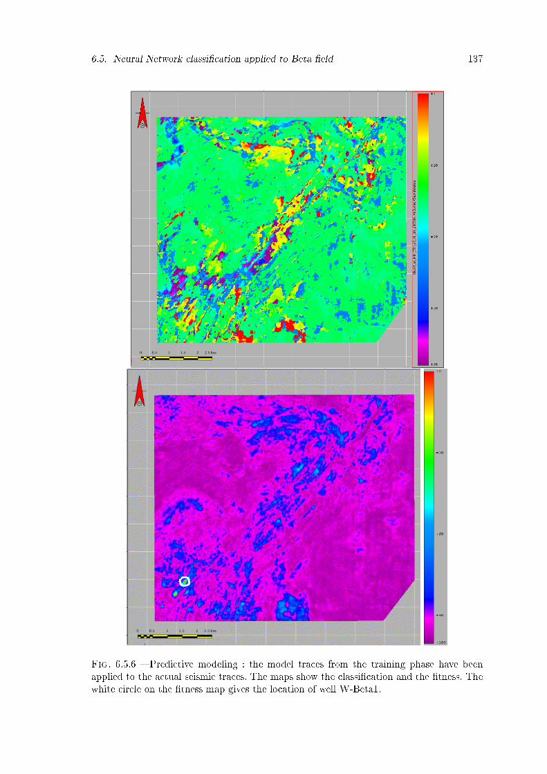
6.5. Neural Network classi�cation applied to Beta �eld 137
Fig. 6.5.6 � Predictive modeling : the model traces from the training phase have beenapplied to the actual seismic traces. The maps show the classi�cation and the �tness. Thewhite circle on the �tness map gives the location of well W-Beta1.
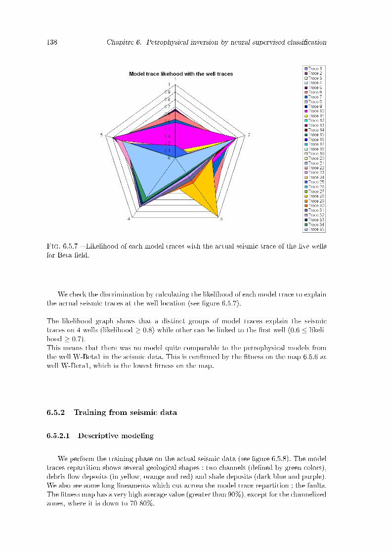
138 Chapitre 6. Petrophysical inversion by neural supervised classi�cation
Fig. 6.5.7 � Likelihood of each model traces with the actual seismic trace of the �ve wellsfor Beta �eld.
We check the discrimination by calculating the likelihood of each model trace to explainthe actual seismic traces at the well location (see �gure 6.5.7).The likelihood graph shows that a distinct groups of model traces explain the seismictraces on 4 wells (likelihood ≥ 0.8) while other can be linked to the �rst well (0.6 ≤ likeli-hood ≥ 0.7).This means that there was no model quite comparable to the petrophysical models fromthe well W-Beta1 in the seismic data. This is con�rmed by the �tness on the map 6.5.6 atwell W-Beta1, which is the lowest �tness on the map.
6.5.2 Training from seismic data
6.5.2.1 Descriptive modeling
We perform the training phase on the actual seismic data (see �gure 6.5.8). The modeltraces repartition shows several geological shapes : two channels (de�ned by green colors),debris �ow deposits (in yellow, orange and red) and shale deposits (dark blue and purple).We also see some long lineaments which cut across the model trace repartition : the faults.The �tness map has a very high average value (greater than 90%), except for the channelizedzones, where it is down to 70-80%.
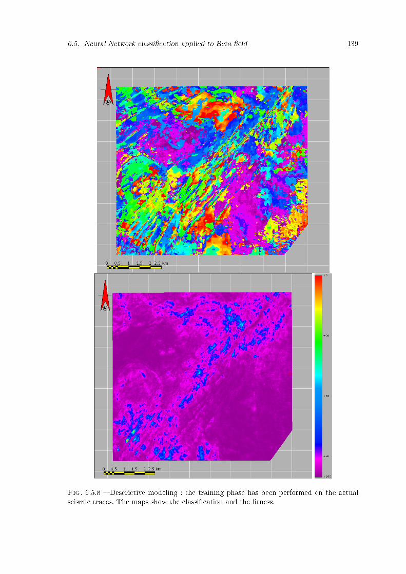
6.5. Neural Network classi�cation applied to Beta �eld 139
Fig. 6.5.8 � Descrictive modeling : the training phase has been performed on the actualseismic traces. The maps show the classi�cation and the �tness.
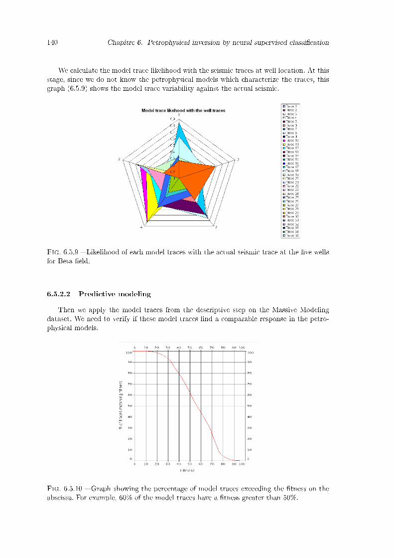
140 Chapitre 6. Petrophysical inversion by neural supervised classi�cation
We calculate the model trace likelihood with the seismic traces at well location. At thisstage, since we do not know the petrophysical models which characterize the traces, thisgraph (6.5.9) shows the model trace variability against the actual seismic.
Fig. 6.5.9 � Likelihood of each model traces with the actual seismic trace at the �ve wellsfor Beta �eld.
6.5.2.2 Predictive modelingThen we apply the model traces from the descriptive step on the Massive Modeling
dataset. We need to verify if these model traces �nd a comparable response in the petro-physical models.
Fig. 6.5.10 � Graph showing the percentage of model traces exceeding the �tness on theabscissa. For example, 60% of the model traces have a �tness greater than 50%.
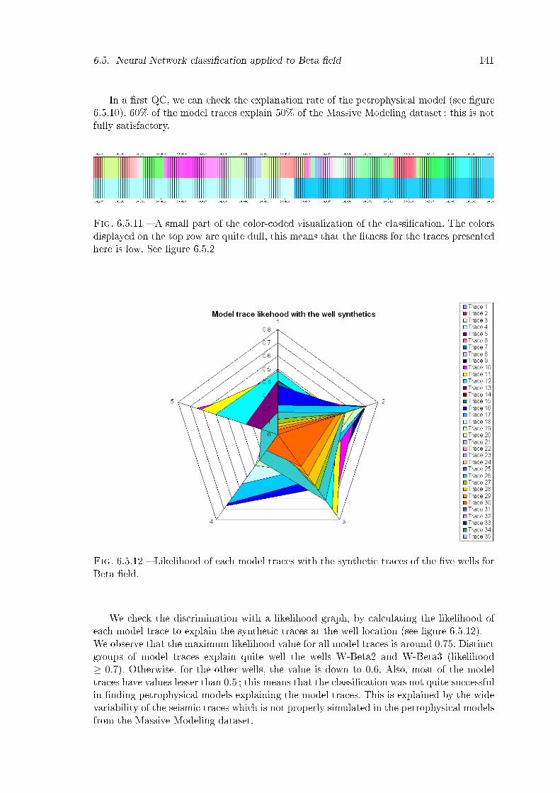
6.5. Neural Network classi�cation applied to Beta �eld 141
In a �rst QC, we can check the explanation rate of the petrophysical model (see �gure6.5.10). 60% of the model traces explain 50% of the Massive Modeling dataset ; this is notfully satisfactory.
Fig. 6.5.11 � A small part of the color-coded visualization of the classi�cation. The colorsdisplayed on the top row are quite dull, this means that the �tness for the traces presentedhere is low. See �gure 6.5.2
Fig. 6.5.12 � Likelihood of each model traces with the synthetic traces of the �ve wells forBeta �eld.
We check the discrimination with a likelihood graph, by calculating the likelihood ofeach model trace to explain the synthetic traces at the well location (see �gure 6.5.12).We observe that the maximum likelihood value for all model traces is around 0.75. Distinctgroups of model traces explain quite well the wells W-Beta2 and W-Beta3 (likelihood≥ 0.7). Otherwise, for the other wells, the value is down to 0.6. Also, most of the modeltraces have values lesser than 0.5 ; this means that the classi�cation was not quite successfulin �nding petrophysical models explaining the model traces. This is explained by the widevariability of the seismic traces which is not properly simulated in the petrophysical modelsfrom the Massive Modeling dataset.
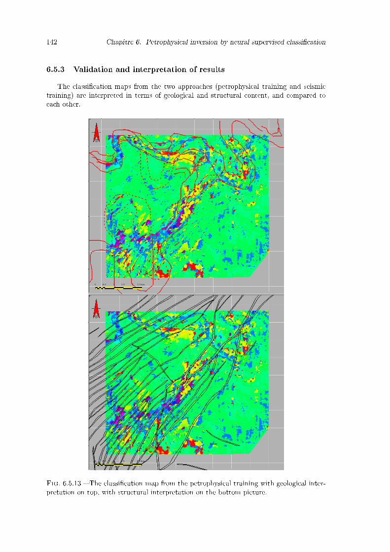
142 Chapitre 6. Petrophysical inversion by neural supervised classi�cation
6.5.3 Validation and interpretation of resultsThe classi�cation maps from the two approaches (petrophysical training and seismic
training) are interpreted in terms of geological and structural content, and compared toeach other.
Fig. 6.5.13 � The classi�cation map from the petrophysical training with geological inter-pretation on top, with structural interpretation on the bottom picture.

6.5. Neural Network classi�cation applied to Beta �eld 143
Fig. 6.5.14 � The classi�cation map from the seismic training with geological interpretationon the top, with structural interpretation on the bottom.

144 Chapitre 6. Petrophysical inversion by neural supervised classi�cation
Geological and structural interpretations provided by geologists were overlaid on bothmaps.
On the map 6.5.13, the channels interpreted on the data are very well de�ned by themodel traces (bluish and purple colors). The debris �ow deposits inside the channels andin the crescent-shaped area (top-middle in the �gure) are fairly well de�ned by the redto yellow model traces. A large area of the map is green, which correspond to the shaledeposits. The structural interpretation shows that some of the faults can be seen in theclassi�cation map (such as the top-left and bottom-left area of the map).On the map 6.5.14, the channels are fairly well de�ned by the model traces (green andlight blue colors). The debris �ow deposits inside the channels and in the crescent-shapedarea are very well de�ned by the red and orange model traces. The shale deposits arecharacterized by several model traces (from dark blue to purple colors) with very widecoherent zones. The structural interpretation of this map shows that most of the faults canbe seen in the classi�cation map.The classi�cation map, from the seismic training, actually shows some variability (seve-ral distinct model traces) for the shale deposits, whereas the classi�cation map from thepetrophysical training explains the shales with very similar model traces (green colors).This was to be expected, since the �ve wells from the �eld were drilled in di�erent channelsequences. The petrophysical models for shales could not be derived from the geostatisticalvariability given by the wells.

6.6. Data Preparation for the Gamma Field 145
6.6 Data Preparation for the Gamma FieldThe same methodology is now applied to the Gamma Field, a carbonate �eld constrai-
ned by several wells.The data being con�dential, they are not fully described in this chapter.The interval of interest is 50ms thick. The geology shows a layer-cake model with threemain facies : dolomites, limestones and anhydrites with low petrophysical variability. Theobjective of this study is to see if seismic facies can be discriminated by the methodology.
6.6.1 Well log preparation6.6.1.1 Well log blocking
The original logs consist in P and S velocities and densities at a 1m sampling step. Weneed to block the logs at the stratigraphic scale to reduce the number of parameters tohandle for the optimization. The geological interpretation provides only two stratigraphicmarkers for each well : the top and the bottom of the interval of interest. Therefore weneed to create other markers with a well segmentation method. This is done by partitio-ning log data into segments and using the mean value of the data points falling withinthe segment to represent the original data. In order to accurately represent the originaldata, each segment is allowed to have arbitrary length. In this way, areas where data pointshave low variation will be represented by a single segment while areas where data pointshave high variation will have many segments. The quality of each segment is evaluated ina least-square sense (Himberg et al. 2001).We create 19 new markers (i.e. 20 macro-layers) for each well. By creating these newmarkers, we increase the probability of introducing variability for the Massive Modelingstep, since the well segmentation approach relies on log shape.An example of results for this blocking step is shown on one of the wells in �gure 6.6.1,where the synthetic of the blocked logs is compared with the actual near seismic.
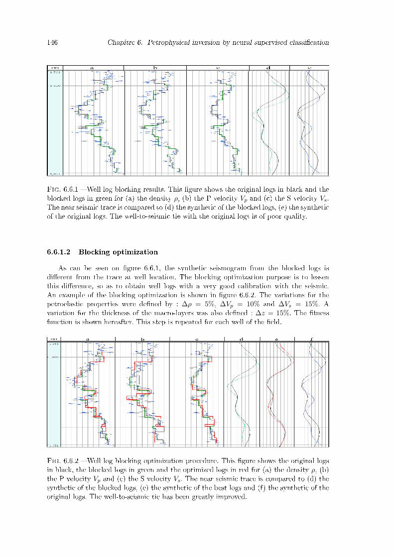
146 Chapitre 6. Petrophysical inversion by neural supervised classi�cation
Fig. 6.6.1 � Well log blocking results. This �gure shows the original logs in black and theblocked logs in green for (a) the density ρ, (b) the P velocity Vp and (c) the S velocity Vs.The near seismic trace is compared to (d) the synthetic of the blocked logs, (e) the syntheticof the original logs. The well-to-seismic tie with the original logs is of poor quality.
6.6.1.2 Blocking optimizationAs can be seen on �gure 6.6.1, the synthetic seismogram from the blocked logs is
di�erent from the trace at well location. The blocking optimization purpose is to lessenthis di�erence, so as to obtain well logs with a very good calibration with the seismic.An example of the blocking optimization is shown in �gure 6.6.2. The variations for thepetroelastic properties were de�ned by : ∆ρ = 5%, ∆Vp = 10% and ∆Vs = 15%. Avariation for the thickness of the macro-layers was also de�ned : ∆z = 15%. The �tnessfunction is shown hereafter. This step is repeated for each well of the �eld.
Fig. 6.6.2 � Well log blocking optimization procedure. This �gure shows the original logsin black, the blocked logs in green and the optimized logs in red for (a) the density ρ, (b)the P velocity Vp and (c) the S velocity Vs. The near seismic trace is compared to (d) thesynthetic of the blocked logs, (e) the synthetic of the best logs and (f) the synthetic of theoriginal logs. The well-to-seismic tie has been greatly improved.

6.6. Data Preparation for the Gamma Field 147
6.6.1.3 Massive ModelingFigure 6.6.3 shows the properties and synthetics of a small part of the Massive Modeling
volume which was generated from the wells of the �eld. Each 50 traces, an actual well hasbeen replaced in the simulation.
Fig. 6.6.3 � The Massive Modeling. The sections are respectively ρ, Vp, Vs and the syntheticseismograms.
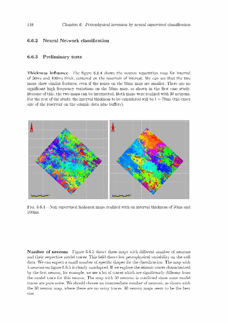
148 Chapitre 6. Petrophysical inversion by neural supervised classi�cation
6.6.2 Neural Network classi�cation
6.6.3 Preliminary tests
Thickness in�uence The �gure 6.6.4 shows the neuron repartition map for intervalof 50ms and 100ms thick, centered on the reservoir of interest. We can see that the twomaps show similar features, even if the zones on the 50ms map are smaller. There are nosigni�cant high frequency variations on the 50ms map, as shown in the �rst case study.Because of this, the two maps can be interpreted. Both maps were realized with 30 neurons.For the rest of the study, the interval thickness to be considered will be t = 70ms (the exactsize of the reservoir on the seismic data plus bu�ers).
Fig. 6.6.4 � Non supervised Kohonen maps realized with an interval thickness of 50ms and100ms.
Number of neurons Figure 6.6.5 shows three maps with di�erent number of neuronsand their respective model traces. This �eld shows low petrophysical variability on the welldata. We can expect a small number of speci�c shapes for the classi�cation. The map with5 neurons on �gure 6.6.5 is clearly unadapted. If we explore the seismic traces characterizedby the �rst neuron, for example, we see a lot of traces which are signi�cantly di�erent fromthe model trace for this neuron. The map with 50 neurons is over�tted since some modeltraces are pure noise. We should choose an intermediate number of neurons, as shown withthe 30 neuron map, where there are no noisy traces. 30 neuron maps seem to be the bestsize.

6.6. Data Preparation for the Gamma Field 149
Fig. 6.6.5 � Non supervised Kohonen maps with respectively 5, 30 and 50 neurons. Nextto each map, we show the resulting neurons (for the 50 neurons map, we show only thesecond half). Some traces from the 50 neurons map represent noise.
Neighbourhood radius The petrophysical variability of the �eld implies a small numberof speci�c trace shapes. But we would like to have as many shapes as possible to be able todiscriminate between facies. We should have a very small neighbourhood radius, this way,the network can �nd di�erent shapes. This is illustrated on �gure 6.6.6 with neighbourhoodradius of 1 and 10 neurons. We can see that between the two tests, the neurons (line 2) arevery similar. This means that even a radius of 1 is too much for the network. To optimize

150 Chapitre 6. Petrophysical inversion by neural supervised classi�cation
the search for original patterns, we will use a neighbourhood radius of 0, and only thewinning neuron will be updated in the learning phase.
Fig. 6.6.6 � Non supervised Kohonen maps realized with neighbourhood radius of 1 and10 neurons. The �rst line shows the neuron repartition, the second line the neurons. Thelast line shows the �tness.
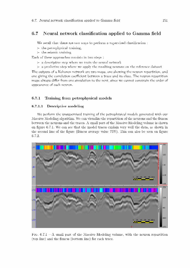
6.7. Neural network classi�cation applied to Gamma �eld 151
6.7 Neural network classi�cation applied to Gamma �eld
We recall that there are two ways to perform a supervised classi�cation :� the petrophysical training,� the seismic training
Each of these approaches consists in two steps :� a descriptive step where we train the neural network� a predictive step where we apply the resulting neurons on the reference dataset
The outputs of a Kohonen network are two maps, one showing the neuron repartition, andone giving the correlation coe�cient between a trace and its class. The neuron repartitionmaps always di�er from one simulation to the next, since we cannot constrain the order ofappearance of each neuron.
6.7.1 Training from petrophysical models6.7.1.1 Descriptive modeling
We perform the unsupervised training of the petrophysical models generated with ourMassive Modeling algorithm. We can visualize the repartition of the neurons and the �tnessbetween the neurons and the traces. A small part of the Massive Modeling volume is shownon �gure 6.7.1. We can see that the model traces explain very well the data, as shown inthe second line of the �gure (�tness average value 75%). This can also be seen on �gure6.7.2.
Fig. 6.7.1 � A small part of the Massive Modeling volume, with the neuron repartition(top line) and the �tness (bottom line) for each trace.
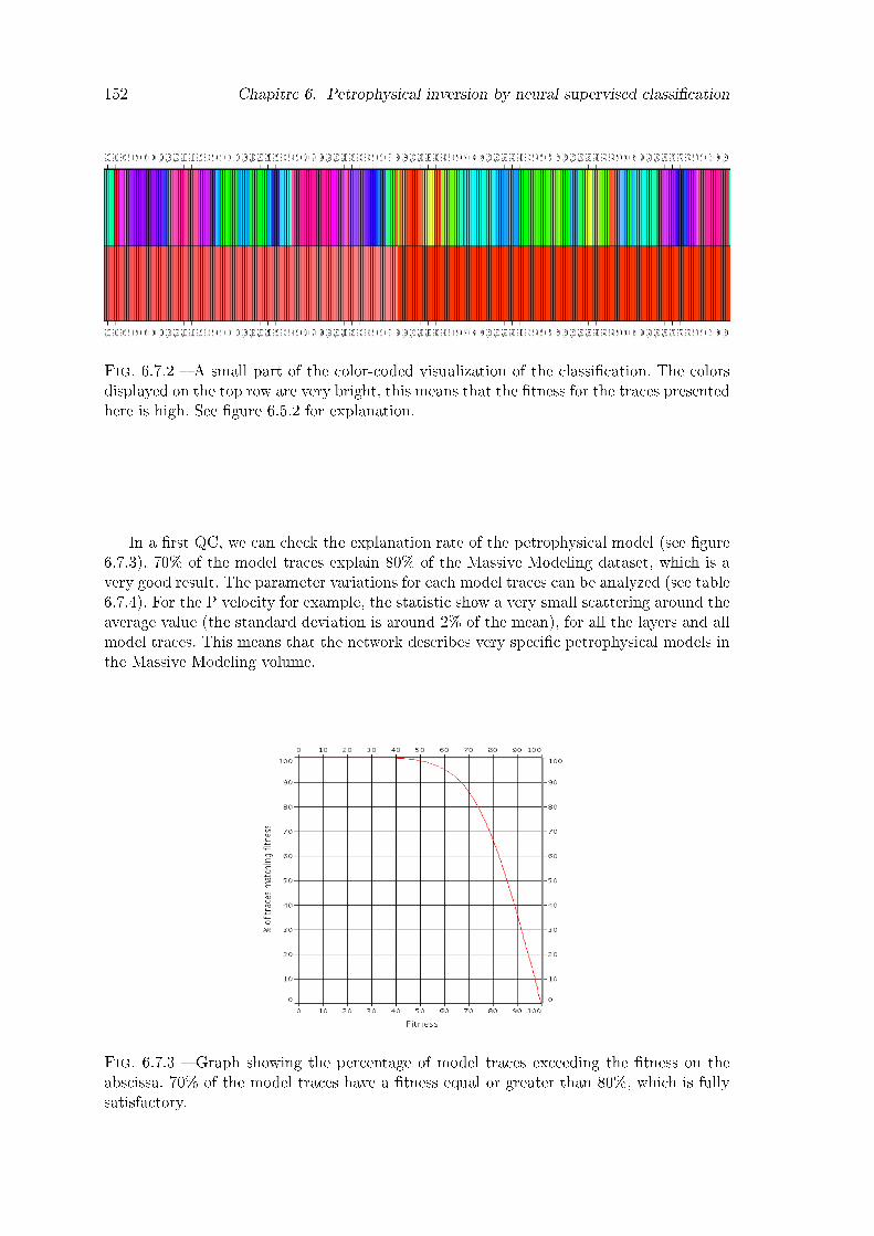
152 Chapitre 6. Petrophysical inversion by neural supervised classi�cation
Fig. 6.7.2 � A small part of the color-coded visualization of the classi�cation. The colorsdisplayed on the top row are very bright, this means that the �tness for the traces presentedhere is high. See �gure 6.5.2 for explanation.
In a �rst QC, we can check the explanation rate of the petrophysical model (see �gure6.7.3). 70% of the model traces explain 80% of the Massive Modeling dataset, which is avery good result. The parameter variations for each model traces can be analyzed (see table6.7.4). For the P velocity for example, the statistic show a very small scattering around theaverage value (the standard deviation is around 2% of the mean), for all the layers and allmodel traces. This means that the network describes very speci�c petrophysical models inthe Massive Modeling volume.
Fig. 6.7.3 � Graph showing the percentage of model traces exceeding the �tness on theabscissa. 70% of the model traces have a �tness equal or greater than 80%, which is fullysatisfactory.
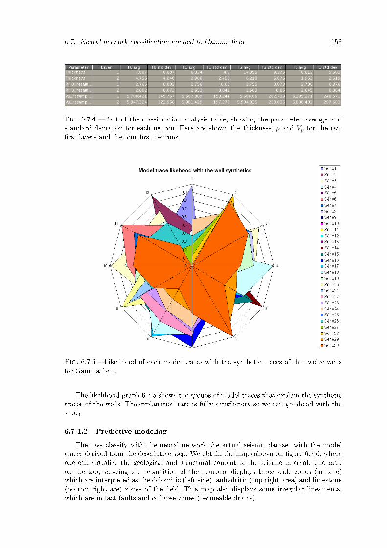
6.7. Neural network classi�cation applied to Gamma �eld 153
Fig. 6.7.4 � Part of the classi�cation analysis table, showing the parameter average andstandard deviation for each neuron. Here are shown the thickness, ρ and Vp for the two�rst layers and the four �rst neurons.
Fig. 6.7.5 � Likelihood of each model traces with the synthetic traces of the twelve wellsfor Gamma �eld.
The likelihood graph 6.7.5 shows the groups of model traces that explain the synthetictraces of the wells. The explanation rate is fully satisfactory so we can go ahead with thestudy.
6.7.1.2 Predictive modelingThen we classify with the neural network the actual seismic dataset with the model
traces derived from the descriptive step. We obtain the maps shown on �gure 6.7.6, whereone can visualize the geological and structural content of the seismic interval. The mapon the top, showing the repartition of the neurons, displays three wide zones (in blue)which are interpreted as the dolomitic (left side), anhydritic (top-right area) and limestone(bottom-right are) zones of the �eld. This map also displays some irregular lineaments,which are in fact faults and collapse zones (permeable drains).
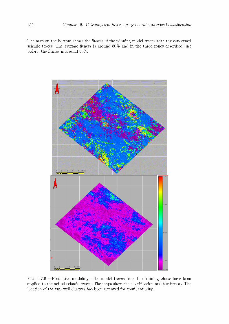
154 Chapitre 6. Petrophysical inversion by neural supervised classi�cation
The map on the bottom shows the �tness of the winning model traces with the concernedseismic traces. The average �tness is around 80% and in the three zones described justbefore, the �tness is around 60%.
Fig. 6.7.6 � Predictive modeling : the model traces from the training phase have beenapplied to the actual seismic traces. The maps show the classi�cation and the �tness. Thelocation of the two well clusters has been removed for con�dentiality.
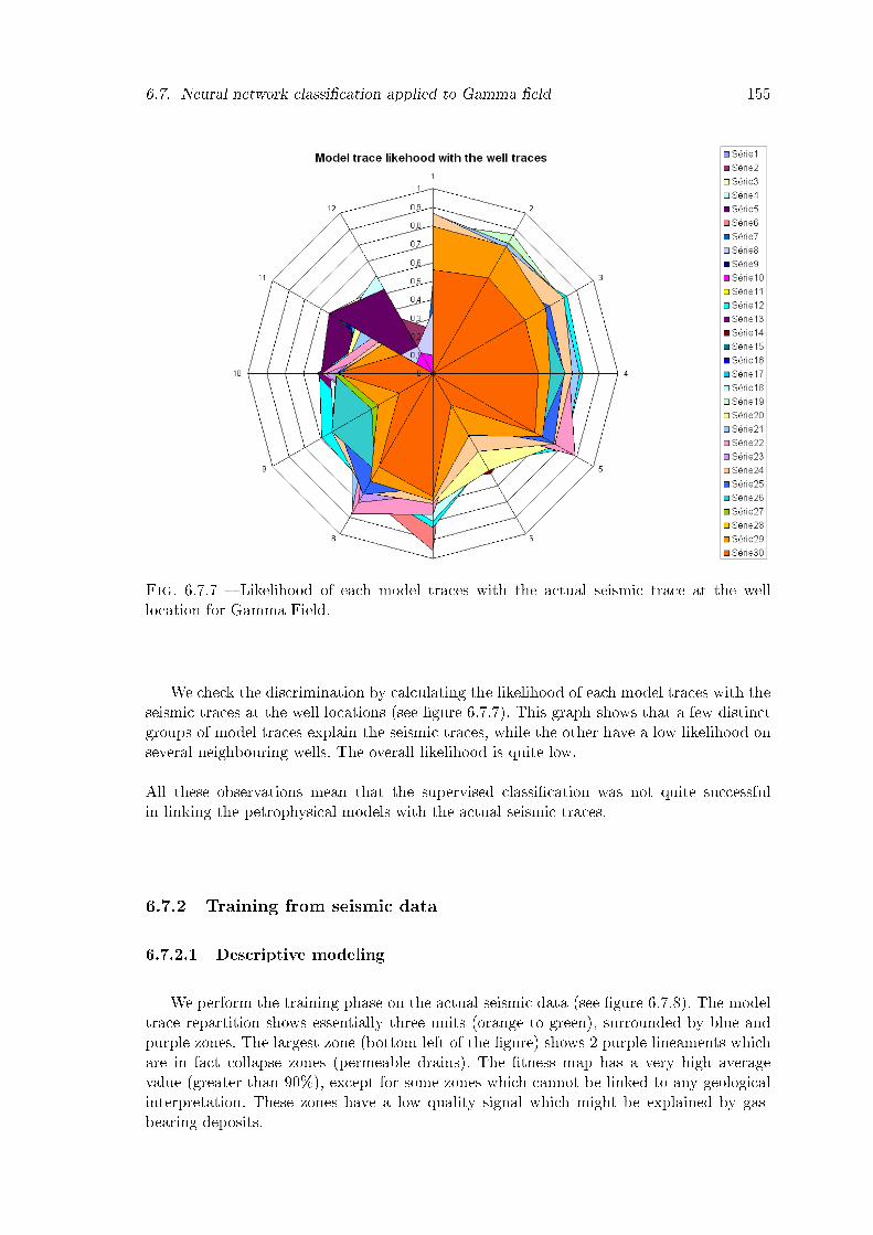
6.7. Neural network classi�cation applied to Gamma �eld 155
Fig. 6.7.7 � Likelihood of each model traces with the actual seismic trace at the welllocation for Gamma Field.
We check the discrimination by calculating the likelihood of each model traces with theseismic traces at the well locations (see �gure 6.7.7). This graph shows that a few distinctgroups of model traces explain the seismic traces, while the other have a low likelihood onseveral neighbouring wells. The overall likelihood is quite low.All these observations mean that the supervised classi�cation was not quite successfulin linking the petrophysical models with the actual seismic traces.
6.7.2 Training from seismic data
6.7.2.1 Descriptive modeling
We perform the training phase on the actual seismic data (see �gure 6.7.8). The modeltrace repartition shows essentially three units (orange to green), surrounded by blue andpurple zones. The largest zone (bottom-left of the �gure) shows 2 purple lineaments whichare in fact collapse zones (permeable drains). The �tness map has a very high averagevalue (greater than 90%), except for some zones which cannot be linked to any geologicalinterpretation. These zones have a low quality signal which might be explained by gas-bearing deposits.

156 Chapitre 6. Petrophysical inversion by neural supervised classi�cation
Fig. 6.7.8 � Descriptive modeling : the training phase has been performed on the actualseismic traces. The maps show the classi�cation and the �tness.
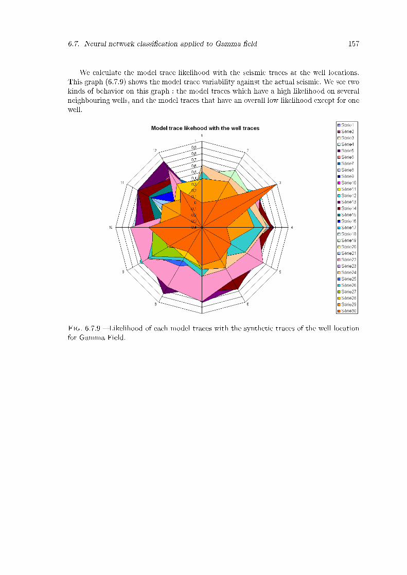
6.7. Neural network classi�cation applied to Gamma �eld 157
We calculate the model trace likelihood with the seismic traces at the well locations.This graph (6.7.9) shows the model trace variability against the actual seismic. We see twokinds of behavior on this graph : the model traces which have a high likelihood on severalneighbouring wells, and the model traces that have an overall low likelihood except for onewell.
Fig. 6.7.9 � Likelihood of each model traces with the synthetic traces of the well locationfor Gamma Field.

158 Chapitre 6. Petrophysical inversion by neural supervised classi�cation
6.7.2.2 Predictive modeling
Then we classify with the neural network the Massive Modeling dataset with the modeltraces derived from the descriptive step, to see if they �nd a comparable seismic responsewithin the generated petrophysical models.
Fig. 6.7.10 � Graph showing the percentage of model traces exceeding the �tness on theabscissa. For example, 70% of the model traces have a �tness greater than 70%.
Fig. 6.7.11 � A small part of the color-coded visualization of the classi�cation. The colorsof some groups of traces displayed on the top row are quite dull, this means that the �tnessfor these traces is low. See �gure 6.5.2 for explanation.
The explanation rate of the Petrophysical models, provided by the �gure 6.7.10 is veryhigh : 70% of the model traces have a �tness greater than 70%, which is fully satisfactory.The �gure 6.7.11 shows that in spite of the high explanation rate, some area have a verylow �tness.

6.7. Neural network classi�cation applied to Gamma �eld 159
Fig. 6.7.12 � Likelihood of each model traces with the synthetic traces of the twelve wellsfor Gamma �eld.
The �nal step is to check the likelihood of the seismic model traces to explain the pe-trophysical models from the Massive Modeling dataset (see �gure 6.7.12).We observe that the maximum likelihood value for all model traces is around 1. We observetwo kinds of behaviour on this �gure : the model traces either have a very high likelihoodwith the well synthetics, or they have a average �tness for all the wells. For the latter,this means that the seismic data contains more variability than the petrophysical modelsfrom the Massive Modeling volume, discriminated by the predictive modeling. There are 2clusters of wells in the Gamma �eld. They actually represent two families of very similarpetrophysical properties. The seismic data contains variabilities which were not sampledby the wells.

160 Chapitre 6. Petrophysical inversion by neural supervised classi�cation
6.7.3 Validation and interpretation of resultsThe classi�cation maps obtained in the two approaches (petrophysical training and
seismic training) are interpreted in terms of geological and structural content, and comparedto each other.
Fig. 6.7.13 � The classi�cation map from the petrophysical training with geological inter-pretation on top, with structural interpretation on the bottom picture.
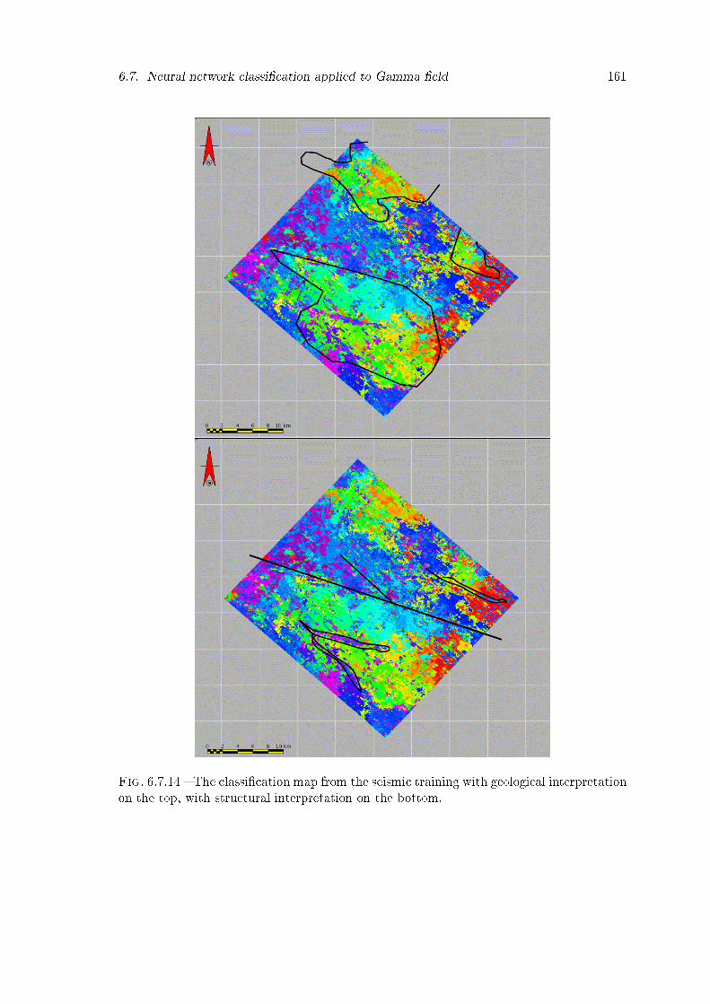
6.7. Neural network classi�cation applied to Gamma �eld 161
Fig. 6.7.14 � The classi�cation map from the seismic training with geological interpretationon the top, with structural interpretation on the bottom.

162 Chapitre 6. Petrophysical inversion by neural supervised classi�cation
Geological and structural interpretations provided by geologists were overlaid on bothmaps.On the map 6.7.13, three wide zones are identi�ed by the blue model traces. These zones areinterpreted as the dolomitic (left side), anhydritic (top-right area) and limestone (bottom-right area) dominant facies zones, but the classi�cation map does not show any variabilitybetween them. The structural interpretation shows that the faults and collapse zones canbe seen in the classi�cation map.On the map 6.7.14, three zones are identi�ed by the red to green model traces. We thinkthat these zones correspond to dominant facies signatures which are interpreted as thedolomitic (left side), anhydritic (top-right area) and limestone (bottom-right area) domi-nant facies. The structural interpretation of this map shows that the faults can be seen inthe classi�cation map, and the main collapse zones (permeable drains) are de�ned by thepurple model traces.The classi�cation map, from the seismic training, actually shows more variability (severaldistinct model traces) on the whole map, whereas the classi�cation map from the petro-physical training shows only some of the model traces. This was to be expected, since onlyspeci�c petrophysical models have been generated with the two well clusters. The missingpetrophysical models could not be derived from the geostatistical variability given by thewells.
6.8. Concluding remarks and perspectives 163
6.8 Concluding remarks and perspectivesExtensive 1D-modeling was carried out to comprehend trace shape variations due to
petrophysical variability. This was fundamental to assign a realistic realisation of propertiesto each seismic trace.The �rst step is to simulate all possible petrophysical models, and to do so we extendthe well database, by creating as many pseudo-wells as needed with an improved MassiveModeling scheme. We generate all possible 1D models through geostatistical simulationsfrom the wells.The next step is to use neural networks which train on the variety of waveforms and ge-nerates a series of model traces called neurons that best represent the diversity of shapes.Seismic traces extracted over a time interval are input to the classi�cation process.Rigorous study of this technique on two 3D datasets with di�erent geological settingshas produced promising results to derive properties that could be used in a reservoir mo-deling sense. On the clastic case, the geological bodies were identi�ed by the methodology.A seismic facies interpretation was also possible on these data. On the carbonate case, amacro-facies interpretation has been done, and the collapse zones identi�ed.The choice of parameters for our methodology is highly data-dependent, but tools areavailable to quantify their e�ect, and guide the user through the study.We are currently implementing the last step of our methodology, where we get the pe-trophysical models assigned to each seismic trace.

164 Chapitre 6. Petrophysical inversion by neural supervised classi�cation

Partie III
Conclusions et perspectives
165

Concluding remarks and future research
This thesis is dedicated to developing innovative approaches in reservoir characteriza-tion, while focusing on the dynamic grid as information support. Traditional techniquesare essentially based on the �ne geological model. The dynamic reservoir model is thenderived after an upscaling phase. Despite technological advances, this upscaling phase isstill a problem since it causes petrophysical bias, particularly on the dynamic properties.We therefore propose a complementary approach that consists in working directly on thereservoir grid to reduce the uncertainties on the static properties, without using the geolo-gical model. The dynamic modeling step on the reservoir model is mainly a�ected by theerrors on the dynamic properties. Methods arising from this approach are presented hereand have been validated on several case studies.
The work of this thesis have resulted in algorithms and tools programmed in Java andimplemented in SISMAGE r©, the seismic interpretation platform developed by TOTAL.
Outcomes of this thesisStructural uncertainty e�ects in reservoir models
The traditional validation work�ows for reservoir models are a�ected by errors of variousorigins. In the �rst part of the thesis, we have illustrated the importance of knowing thegeometry of the reservoir prior to the stratigraphic inversion. To see the impact of structuraluncertainty in a traditional reservoir characterization study, we generated not one butseveral models, all consistent with the local geology. We then inverted the seismic dataand conducted a petrophysical classi�cation of the resulting attributes. Facies have beeninterpreted in the reservoir models, which were analyzed in a systematic way. Taking intoaccount structural uncertainties can help assess their e�ect on the repartition of facies inthe reservoir grid.
Scale change problematicTraditional reservoir characterization methods use seismic data to constrain the model.
These data, which re�ect property contrasts between stratigraphic layers, are the onlysource of information that covers the entire reservoir. The actual values of the propertiesare only known at the well locations.Furthermore, the attributes derived from seismic data are at a di�erent scale from that ofthe reservoir and we need to either operate a scale change of these attributes, with all theproblems associated to upscaling, or simulate reservoir properties using the attributes assecondary variables. We propose two innovative approaches in reservoir characterization,
167
168 Concluding remarks and future research
taking into account di�erent scales of observation ; these approaches form the essentialwork of this thesis.
Gradual deformation inversionWe address the problem of scale changes using a geostatistical simulation method : the
gradual deformation. This method has been developed in other contexts, for example inhistory matching, but here it is applied for the �rst time to seismic data inversion. Thisprocess of inversion is used to generate seismic attributes directly at the reservoir scale,with well conditioning, and with an objective function based on seismic comparison.
Petrophysical inversion with neural supervised classi�cationNeural networks can handle a very large number of parameters poorly constrained
by data at di�erent scales. The basic geological information is provided by well data,blocked at the reservoir scale and constrained by seismic data. Well data are the only directaccess to reservoir properties, but are in insu�cient volume to characterize the entire 3Dseismic block. We generate a reference population with the help of the Massive Modelingwhich creates thousands of synthetic logs by geostatistical interpolation between wells. Weuse unsupervised neural networks (Kohonen maps) in two phases : the learning phase onthe reference population, then the supervised classi�cation on actual data. The resultingmaps allow the delineation of large areas, according to their petrophysical properties. Thiszonation is consistent with geological interpretation carried out independently.The originality of our approach lies in the reconciliation the well, seismic and reservoirscales, made possible by neural supervised classi�cation. We validated the method on clasticand carbonate reservoirs.
Future workOur work was developed in pursuit of operational e�ciency. This led to inevitable
simpli�cations. For example, the method for seismic modeling is deliberately simplistic(multi-1D convolution) to be as interactive as possible.The methods developed in this thesis have been tested and validated on three actual casestudies chosen for their geological diversity. It will be interesting to test these methodson other cases to ensure their robustness. The approaches are complemented with toolsto discuss the validity of results. All the tools are operational and will remain in constantevolution.
Possible improvementsThe gradual deformation inversion remains a product which could be improved :� Optimization of property space exploration : we have used the basic formulation of
the gradual deformation. It may be replaced by a more sophisticated approach thatuses several secondary realizations and a gradient search (Hu and Ravalec-Dupin2004).
� Optimization based on actual seismic data : the processes were constrained by syn-thetic data, calculated from previous inversion results providing "solutions" to com-pare our property realizations. The next step will be to directly use the actual data.
169
� Using a petroelastic model : the current processes recover the density and seismicvelocities. The implementation may include a PEM to recover the petrophysicalproperties.
The petrophysical inversion by neural supervised classi�cation could be complemented bya process assigning the best suited petrophysical model to each seismic trace.We have seen that in our Massive Modeling approach, the new petrophysical models weregenerated by SGS, by continuous variations of properties and thickness of layers. This iswell suited for a tabular geology (as the Gamma �eld), but not for a complex geology (Beta�eld) showing channels, pinch-outs or other discontinuous geological objects. It would beinteresting to improve the Massive Modeling by integrating the stratigraphic interpretationto model variations that would follow the geology.Finally, other tools for analyzing the petrophysical discrimination could be envisagedto facilitate the understanding of petrophysics-seismic relationships. We can suggest, forexample, the reorganization of the traces of the learning volume based on the model traceand correlation, or the generation of Hφ graphs.
Seismic reservoir characterization is an important discipline in exploration and �elddevelopment with applications from prospect identi�cation to detailed reservoir delineation,including reservoir geometry, reservoir lithology, sealing capability and reservoir quality. Toimprove the accuracy of reservoir property prediction and minimize the uncertainties, weneed to explore the geological, geophysical and reservoir domains, use many methods, andintegrate several types of data at di�erent scales. The work done during this thesis allowedus to understand the di�culty of going back to petrophysical properties. The resolution ofthis issue remains the main challenge for geophysical exploration in the future.


Annexes
171


Annexe 1 : SEG Annual Conference (SanAntonio 2007
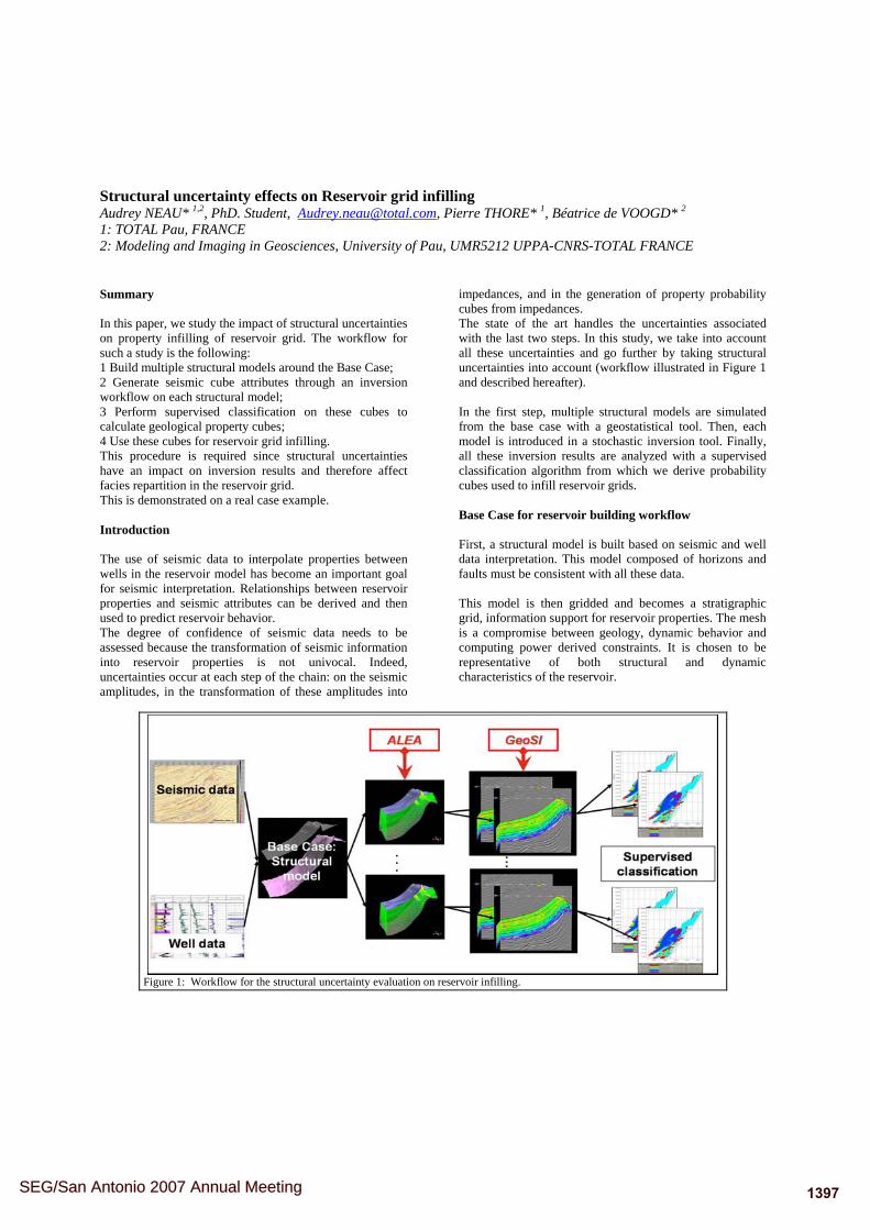
Structural uncertainty effects on Reservoir grid infilling Audrey NEAU* 1,2, PhD. Student, [email protected], Pierre THORE* 1, Béatrice de VOOGD* 2
1: TOTAL Pau, FRANCE 2: Modeling and Imaging in Geosciences, University of Pau, UMR5212 UPPA-CNRS-TOTAL FRANCE Summary In this paper, we study the impact of structural uncertainties on property infilling of reservoir grid. The workflow for such a study is the following: 1 Build multiple structural models around the Base Case; 2 Generate seismic cube attributes through an inversion workflow on each structural model; 3 Perform supervised classification on these cubes to calculate geological property cubes; 4 Use these cubes for reservoir grid infilling. This procedure is required since structural uncertainties have an impact on inversion results and therefore affect facies repartition in the reservoir grid. This is demonstrated on a real case example. Introduction The use of seismic data to interpolate properties between wells in the reservoir model has become an important goal for seismic interpretation. Relationships between reservoir properties and seismic attributes can be derived and then used to predict reservoir behavior. The degree of confidence of seismic data needs to be assessed because the transformation of seismic information into reservoir properties is not univocal. Indeed, uncertainties occur at each step of the chain: on the seismic amplitudes, in the transformation of these amplitudes into
impedances, and in the generation of property probability cubes from impedances. The state of the art handles the uncertainties associated with the last two steps. In this study, we take into account all these uncertainties and go further by taking structural uncertainties into account (workflow illustrated in Figure 1 and described hereafter). In the first step, multiple structural models are simulated from the base case with a geostatistical tool. Then, each model is introduced in a stochastic inversion tool. Finally, all these inversion results are analyzed with a supervised classification algorithm from which we derive probability cubes used to infill reservoir grids. Base Case for reservoir building workflow First, a structural model is built based on seismic and well data interpretation. This model composed of horizons and faults must be consistent with all these data. This model is then gridded and becomes a stratigraphic grid, information support for reservoir properties. The mesh is a compromise between geology, dynamic behavior and computing power derived constraints. It is chosen to be representative of both structural and dynamic characteristics of the reservoir.
Figure 1: Workflow for the structural uncertainty evaluation on reservoir infilling.
1397SEG/San Antonio 2007 Annual Meeting
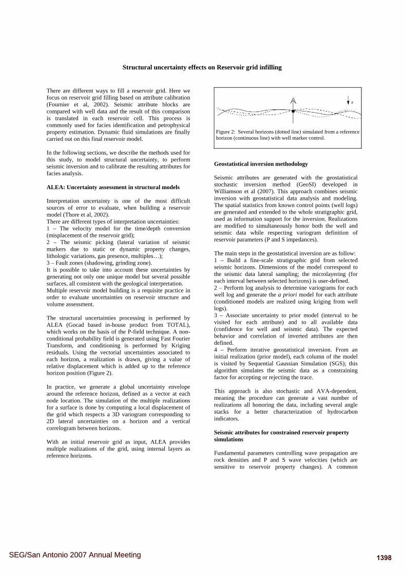
Structural uncertainty effects on Reservoir grid infilling
There are different ways to fill a reservoir grid. Here we focus on reservoir grid filling based on attribute calibration (Fournier et al, 2002). Seismic attribute blocks are compared with well data and the result of this comparison is translated in each reservoir cell. This process is commonly used for facies identification and petrophysical property estimation. Dynamic fluid simulations are finally carried out on this final reservoir model. In the following sections, we describe the methods used for this study, to model structural uncertainty, to perform seismic inversion and to calibrate the resulting attributes for facies analysis. ALEA: Uncertainty assessment in structural models Interpretation uncertainty is one of the most difficult sources of error to evaluate, when building a reservoir model (Thore et al, 2002). There are different types of interpretation uncertainties: 1 – The velocity model for the time/depth conversion (misplacement of the reservoir grid); 2 – The seismic picking (lateral variation of seismic markers due to static or dynamic property changes, lithologic variations, gas presence, multiples…); 3 – Fault zones (shadowing, grinding zone). It is possible to take into account these uncertainties by generating not only one unique model but several possible surfaces, all consistent with the geological interpretation. Multiple reservoir model building is a requisite practice in order to evaluate uncertainties on reservoir structure and volume assessment. The structural uncertainties processing is performed by ALEA (Gocad based in-house product from TOTAL), which works on the basis of the P-field technique. A non-conditional probability field is generated using Fast Fourier Transform, and conditioning is performed by Kriging residuals. Using the vectorial uncertainties associated to each horizon, a realization is drawn, giving a value of relative displacement which is added up to the reference horizon position (Figure 2). In practice, we generate a global uncertainty envelope around the reference horizon, defined as a vector at each node location. The simulation of the multiple realizations for a surface is done by computing a local displacement of the grid which respects a 3D variogram corresponding to 2D lateral uncertainties on a horizon and a vertical correlogram between horizons. With an initial reservoir grid as input, ALEA provides multiple realizations of the grid, using internal layers as reference horizons.
Geostatistical inversion methodology Seismic attributes are generated with the geostatistical stochastic inversion method (GeoSI) developed in Williamson et al (2007). This approach combines seismic inversion with geostatistical data analysis and modeling. The spatial statistics from known control points (well logs) are generated and extended to the whole stratigraphic grid, used as information support for the inversion. Realizations are modified to simultaneously honor both the well and seismic data while respecting variogram definition of reservoir parameters (P and S impedances). The main steps in the geostatistical inversion are as follow: 1 – Build a fine-scale stratigraphic grid from selected seismic horizons. Dimensions of the model correspond to the seismic data lateral sampling; the microlayering (for each interval between selected horizons) is user-defined. 2 – Perform log analysis to determine variograms for each well log and generate the a priori model for each attribute (conditioned models are realized using kriging from well logs). 3 – Associate uncertainty to prior model (interval to be visited for each attribute) and to all available data (confidence for well and seismic data). The expected behavior and correlation of inverted attributes are then defined. 4 – Perform iterative geostatistical inversion. From an initial realization (prior model), each column of the model is visited by Sequential Gaussian Simulation (SGS); this algorithm simulates the seismic data as a constraining factor for accepting or rejecting the trace. This approach is also stochastic and AVA-dependent, meaning the procedure can generate a vast number of realizations all honoring the data, including several angle stacks for a better characterization of hydrocarbon indicators. Seismic attributes for constrained reservoir property simulations Fundamental parameters controlling wave propagation are rock densities and P and S wave velocities (which are sensitive to reservoir property changes). A common
Figure 2: Several horizons (dotted line) simulated from a reference horizon (continuous line) with well marker control.
1398SEG/San Antonio 2007 Annual Meeting

Structural uncertainty effects on Reservoir grid infilling
attribute for reservoir characterization is impedance (product of density and velocity), either acoustic or elastic, which contains relationships between rock physics and seismic (Mukerji et al, 2001). From the multiple realizations of GeoSI, we use P and S impedances to calibrate attributes. Relationships, between petroelastical (impedances) and petrophysical (facies) reservoir properties are analyzed at wells. They are reviewed at seismic scale by extracting minicubes around well locations. The cross-plot Ip-Is colored by facies (or other property) at the well is divided into different parts. These parts must be as homogeneous as possible in the domain delimited by the attributes. The different zones revealed by the cross-plot are projected on the seismic cubes to generate geological property cubes. Example from a West African offshore reservoir The reservoir studied is a complex of submarine channel reservoirs. This is a thick Oligocene sequence of silty clays that includes important sandstone reservoirs in deepwater areas. The deposits are mainly turbiditic, with interbedded channel sands. Near, mid, and far offset stacks are available at a resolution of 3 ms over a 4.8 Km x 1.8 Km area. Only one well in the higher part of the structure is available, with raw and interpreted logs. Five major lithofacies are defined from these logs and are used for facies classification (shales (1); laminated sands (2); fine sands (3); coarse sands (4); cimented sands (5)). Reservoir top and bottom surfaces picked from the seismic data are used to build a corner-point stratigraphic grid of 114 x 159 x 113 = 2 048 238 nodes. Panel 1 in Figure 3 shows the initial reservoir grid with well path (red track). The horizontal resolution of the grid ranges from 45 to 70 m. The vertical resolution ranges between 3 and 15 m. Top and bottom layers are extracted from the initial reservoir grid as reference horizons. An uncertainty map (based on seismic picking derived uncertainties) is associated to each of them. With the reference structural model and the uncertainty maps, one hundred equiprobable structural models are generated; two of them are illustrated in Figure 3. The initial grid (Panel 1, Figure 3) is G1, Panel 2 grid is G2 and
Panel 3 grid is G3. G2 top and bottom horizons are globally below initial horizons, whereas G3 top and bottom horizons are globally above initial horizons. A hundred P (IP) and S (IS) impedance cubes are generated for several structural models, using the same layering and the same prior model for each of them. The multiple realizations obtained permit to evaluate reservoir uncertainty. The standard deviation ranges from 5% to 10% around the mean of all realizations. Figure 4 shows the P mean impedance on the 26th layer for each model. Considering the mean impedance for each structural model leads to differences mainly due to structural uncertainties. After validation of the inversion at the well, we are able to go ahead and classify the inversion results. The impedance attribute cubes are then used to estimate the most likely facies by cross-plot analysis. Figure 5 shows the facies classification from the inverted traces compared to the known facies at the well, for each structural model. For each cross-plot, facies are analyzed separately. Except for facies 1 (too much values) and facies 5 (not enough values), we observe that G2 generally has lower IS values (and to a lesser extent, IP too), while G3 displays globally higher IS values. This shows that probability cubes drawn from these classifications are affected by structural uncertainties. Conclusions These results show that structural uncertainty effects need to be assessed on property probability cubes before performing reservoir grid infilling. This has been done by considering not one but a class of structural models, all consistent with the seismic and well data. The approach described here is a practical and functional mean to insert the concept of structural uncertainty in the reservoir modeling workflow. Acknowledgements The authors would like to thank TOTAL for the release of this work for publication. The authors would also like to acknowledge G.R.C. and C.G.G. collaborators for the use of GeoSI software.
1399SEG/San Antonio 2007 Annual Meeting
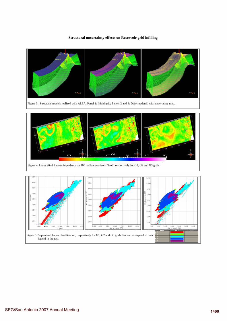
Structural uncertainty effects on Reservoir grid infilling
Figure 3: Structural models realized with ALEA: Panel 1: Initial grid; Panels 2 and 3: Deformed grid with uncertainty map.
Figure 4: Layer 26 of P mean impedance on 100 realizations from GeoSI respectively for G1, G2 and G3 grids.
Figure 5: Supervised facies classification, respectively for G1, G2 and G3 grids. Facies correspond to their legend in the text.
1400SEG/San Antonio 2007 Annual Meeting

EDITED REFERENCES Note: This reference list is a copy-edited version of the reference list submitted by the author. Reference lists for the 2007 SEG Technical Program Expanded Abstracts have been copy edited so that references provided with the online metadata for each paper will achieve a high degree of linking to cited sources that appear on the Web. REFERENCES Fournier, F., P. Y. Dequirez, C. G. Macrides, and M. Rademakers, 2002, Quantitative lithostratigraphic interpretation of seismic
data for characterization of the Unayzah Formation in central Saudi Arabia: Geophysics, 67, 1372–1381 Mukerji, T., P. Avseth, I. Takahashi, and E. F. Gonzalez, 2001, Statistical rock physics: Combining rock physics, information
theory, and geostatistics to reduce uncertainty in seismic reservoir characterization: The Leading Edge, 3, 313–319. Thore, P., A. Shtuka, M. Lecour, T. Ait-Ettajer, and R. Cognot, 2002, Structural uncertainties: Determination, management, and
applications: Geophysics, 67, 840–852. Williamson, P. R., A. J. Cherrett, and R. Bornard, 2007, Geostatistical stochastic elastic inversion - An efficient method for
integrating seismic and well data: Presented at the 69th Conference and Exhibition, EAGE.
1401SEG/San Antonio 2007 Annual Meeting

Annexe 2 : EAGE Annual Conference(Rome 2008)

70th EAGE Conference & Exhibition — Rome, Italy, 9 - 12 June 2008
A045A Genetic Algorithm for Optimal Blocking of WellLogsP. Thore* (TOTAL), G. Morin (NT Conseil) & A. Neau (TOTAL & University ofPau)
SUMMARYBlocking well logs is an initial and mandatory step for many processes. It is an upscaling procedure andhas no unique solution. In order to find a set of "optimal blocking" for geophysical applications wepropose to use a criterion based on seismic difference between synthetic seismogram computed on the finescale logs and synthetic seismogram computed on the blocked logs. The optimisation process is performedwith a genetic algorithm because genetic algorithms have the ability to solve non linear problem and toprovide a set of solutions which gives an idea of the uncertainty in the model space. Thanks to the limitednumber of parameters, blocked well logs can be used lately in many applications such as MassiveModelling.
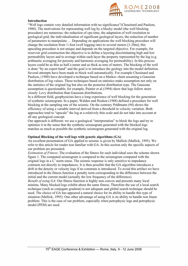
70th EAGE Conference & Exhibition — Rome, Italy, 9 - 12 June 2008
Introduction “Well logs contain very detailed information with no significance”(Chouinard and Paulson, 1988). The motivations for representing well log by a blocky model (the well blocking procedure) are numerous: the reduction of cpu time, the adaptation of well resolution to geological grid, the individualisation of significant geological layers, the reduction of number of parameters to manipulate…. Depending on applications the well blocking procedure will change the resolution from ½ foot (well logging rate) to several meters [1-20m]; this upscaling procedure is not unique and depends on the targeted objective. For example, for reservoir grid construction the objective is to define a layering discriminating high and low permeability layers and to average within each layer the property represented by the log (e.g. arithmetic averaging for porosity and harmonic averaging for permeability). In this process layers could be as thin as half a meter and as thick as tens of meters. The blocking of the well is done “by an expert hand” and the goal is to introduce the geology into the model definition. Several attempts have been made to block well automatically. For example Chouinard and Paulson, (1988) have developed a technique based on a Markov chain assuming a Gaussian distribution of log values. These techniques based on statistics make assumption not only on the statistics of the original log but also on the posterior distribution type. The Gaussian assumption is questionable, for example, Painter et al (1994) show that logs follow more closely Levy distribution than Gaussian distributions. In a different field, geophysicists have a long experience of well blocking for the generation of synthetic seismogram. In a paper, Walden and Hosken (1988) defined a procedure for well blocking at the sampling rate of the seismic. On the contrary Prüßmann (94) shows the efficiency of using a variable interval derived from a threshold in velocity variation. Both approaches tend to “upscale” the log at a relatively thin scale and do not take into account at all any geological concept. Our approach is different: we use a geological “interpretation” to block the logs and try to optimize it in the sense that the synthetic seismogram generated with the blocked logs matches as much as possible the synthetic seismogram generated with the original log. Optimal Blocking of the well logs with genetic algorithms (GA) An excellent presentation of GA applied to seismic is given by Mallick (Mallick, 1995). We refer to this article for reader non familiar with GA. In this section only the specific aspects of our problem are presented. Estimation of Fitness: The evaluation of the fitness for each individual uses the scheme shown figure 1. The computed seismogram is compared to the seismogram computed with the original logs in a L2 norm sense. The seismic response is only sensitive to impedance contrasts not directly to impedances. It is then possible that the GA algorithm introduces a drift in the density or velocity logs if no constrain is introduced. To avoid this artifact we have introduced in the fitness function a penalty term corresponding to the difference between the initial and the current model (actually the low frequency of the difference). Benefit of using GA: Our fitness function is highly non convex and presents many local minima. Many blocked logs exhibit about the same fitness. Therefore the use of a local search technique (such as conjugate gradient) is not adequate and global search technique should be used. The choice of GA has appeared a natural choice for its ability to handle this type of situation (Mallick, 1995). One other advantage of using GA is its ability to handle non linear problem. This is the case of our problem, especially when petrophysic logs and petrophysic model (PEM) are used.
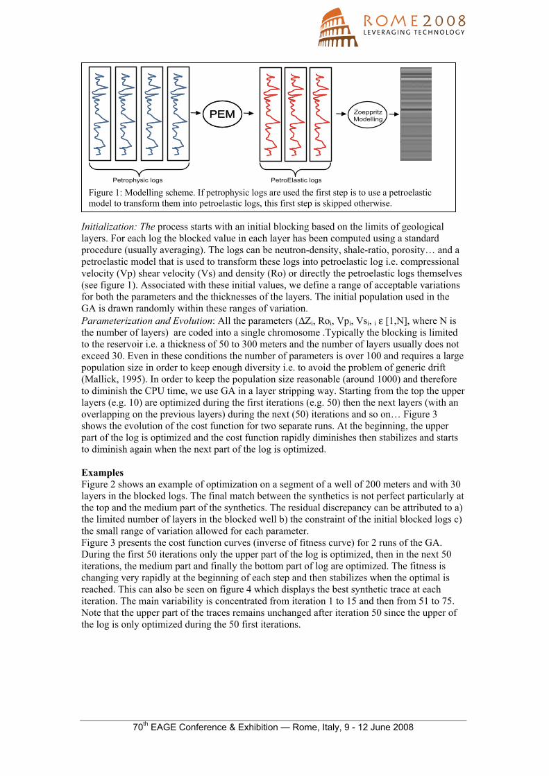
70th EAGE Conference & Exhibition — Rome, Italy, 9 - 12 June 2008
Initialization: The process starts with an initial blocking based on the limits of geological layers. For each log the blocked value in each layer has been computed using a standard procedure (usually averaging). The logs can be neutron-density, shale-ratio, porosity… and a petroelastic model that is used to transform these logs into petroelastic log i.e. compressional velocity (Vp) shear velocity (Vs) and density (Ro) or directly the petroelastic logs themselves (see figure 1). Associated with these initial values, we define a range of acceptable variations for both the parameters and the thicknesses of the layers. The initial population used in the GA is drawn randomly within these ranges of variation. Parameterization and Evolution: All the parameters (ΔZi, Roi, Vpi, Vsi, i ε [1,N], where N is the number of layers) are coded into a single chromosome .Typically the blocking is limited to the reservoir i.e. a thickness of 50 to 300 meters and the number of layers usually does not exceed 30. Even in these conditions the number of parameters is over 100 and requires a large population size in order to keep enough diversity i.e. to avoid the problem of generic drift (Mallick, 1995). In order to keep the population size reasonable (around 1000) and therefore to diminish the CPU time, we use GA in a layer stripping way. Starting from the top the upper layers (e.g. 10) are optimized during the first iterations (e.g. 50) then the next layers (with an overlapping on the previous layers) during the next (50) iterations and so on… Figure 3 shows the evolution of the cost function for two separate runs. At the beginning, the upper part of the log is optimized and the cost function rapidly diminishes then stabilizes and starts to diminish again when the next part of the log is optimized. Examples Figure 2 shows an example of optimization on a segment of a well of 200 meters and with 30 layers in the blocked logs. The final match between the synthetics is not perfect particularly at the top and the medium part of the synthetics. The residual discrepancy can be attributed to a) the limited number of layers in the blocked well b) the constraint of the initial blocked logs c) the small range of variation allowed for each parameter. Figure 3 presents the cost function curves (inverse of fitness curve) for 2 runs of the GA. During the first 50 iterations only the upper part of the log is optimized, then in the next 50 iterations, the medium part and finally the bottom part of log are optimized. The fitness is changing very rapidly at the beginning of each step and then stabilizes when the optimal is reached. This can also be seen on figure 4 which displays the best synthetic trace at each iteration. The main variability is concentrated from iteration 1 to 15 and then from 51 to 75. Note that the upper part of the traces remains unchanged after iteration 50 since the upper of the log is only optimized during the 50 first iterations.
PEMPEM ZoeppritzModelling
Petrophysic logs PetroElastic logs Figure 1: Modelling scheme. If petrophysic logs are used the first step is to use a petroelastic model to transform them into petroelastic logs, this first step is skipped otherwise.

70th EAGE Conference & Exhibition — Rome, Italy, 9 - 12 June 2008
Example of Application: Massive Seismic Modelling (Julien et al 2002) consists in computing the seismic response of a set of pseudo wells. It is used to compute the tuning curves for pre or post stack attributes
Figure 4: Best synthetic trace at each iteration. In the 50 first iterations the upper part of the model is optimized, then the middle part and finally the remaining part. The last 5 traces correspond to the synthetic trace computed with the original logs.
Figure 3: Evolution of the cost function of the best individual at each iteration (two runs of the GA optimisation). The population size is 2000 and the number of layer is 30. In the 50 first iterations, the upper part of the model is optimized, then the middle part in the next 50 and the remaining part in the last 50.
Figure 2: Blue original log, Green original blocking, and Red best individual. Left track density log, centre track velocity log, and left track synthetics.
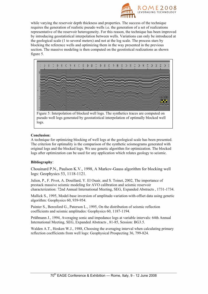
70th EAGE Conference & Exhibition — Rome, Italy, 9 - 12 June 2008
while varying the reservoir depth thickness and properties. The success of the technique requires the generation of realistic pseudo wells i.e. the generation of a set of realizations representative of the reservoir heterogeneity. For this reason, the technique has been improved by introducing geostatistical interpolation between wells. Variations can only be introduced at the geological scale (1 to several meters) and not at the log scale. The process stars by blocking the reference wells and optimizing them in the way presented in the previous section. The massive modeling is then computed on the geostistical realizations as shown figure 5.
Conclusion: A technique for optimizing blocking of well logs at the geological scale has been presented. The criterion for optimality is the comparison of the synthetic seismograms generated with original logs and the blocked logs. We use genetic algorithm for optimization. The blocked logs after optimization can be used for any application which relates geology to seismic. Bibliography:
Chouinard P.N., Paulson K.V., 1998, A Markov-Gauss algorithm for blocking well logs: Geophysics 53, 1118-1121. Julien, P., F. Pivot, A. Douillard, Y. El Ouair, and S. Toinet, 2002, The importance of prestack massive seismic modeling for AVO calibration and seismic reservoir characterization: 72nd Annual International Meeting, SEG, Expanded Abstracts , 1731-1734.
Mallick S., 1995, Model-base inversion of amplitude-variation-with-offset data using genetic algorithm: Geophysics 60, 939-954.
Painter S., Beresford G., Paterson L., 1995, On the distribution of seismic reflection coefficients and seismic amplitudes: Geophysics 60, 1187-1194.
Prüßmann J., 1994, Averaging sonic and impedance logs at variable intervals: 64th Annual International Meeting, SEG, Expanded Abstracts , 81-85, Session: BG3.5.
Walden A.T., Hosken W.J., 1988, Choosing the averaging interval when calculating primary reflection coefficients from well logs: Geophysical Prospecting 36, 799-824.
Figure 5: Interpolation of blocked well logs. The synthetics traces are computed on pseudo well logs generated by geostatistical interpolation of optimally blocked well logs.

Annexe 3 : SEG Annual Conference (LasVegas 2008

Combining the Gradual Deformation Method with Seismic Forward Modeling to constrain ReservoirModelsAudrey NEAU* (1, 2), PhD. Student, Pierre THORE (1), Beatrice de VOOGD (2).1: TOTAL Pau, France2: Modeling and Imaging in Geosciences, UMR5212 UPPA-CNRS-TOTAL, University of Pau, France
SUMMARY
In this paper, we propose a new methodology for seismic inversion atthe reservoir grid scale. The inversion engine adapts the Gradual De-formation Method (GDM) to seismic inversion.GDM is a geostatistical technique, previously used in the field of his-tory matching, that allows to continuously modify reservoir realiza-tions, while preserving spatial variability.The workflow is the following:− Combine the initial petroelastic properties in the reservoir grid withan independent realization, accordingly to the principles of GDM;− Condition the new realization with well logs;− Simulate the synthetic seismic. The misfit between actual and syn-thetic data is given by the objective function;−Minimize the objective function by perturbing the gradual deforma-tion coefficient;− Assign the optimized realization as the new initial one.This loop is performed until the match with the actual seismic data issatisfactory.We show that the basic GDM formulation gives promising results on asynthetic test case for seismic inversion in a reservoir model.
INTRODUCTION
Ensuring consistency between multiscale data for reservoir characteri-zation is an important matter to increase constraints and reduce uncer-tainty in reservoir description.The reservoir flow model must preserve the small-scale informationcontent observed in well logs and the large-scale structure from globalmeasurements such as production data. However, the history-matchingprocess yields non-unique and misleading solutions because a givenproduction curve can be derived from many models with completelydifferent geological structures.
To achieve the best possible history match of production data, thereservoir model must synthesize as much information as possible. Wedecrease the number of possible models by collecting all available ge-ological, geophysical as well as dynamic reservoir information, andintegrate them in the reservoir description.Constraining reservoir properties simulations to seismic data leads tomuch more accurate reservoir models. Due to difference in scale, theinformation derived from seismic data must be upscaled into the reser-voir, leading to much inconsistencies and information losses.
We propose a new methodology to directly recover seismic attributesat reservoir scale, by combining the gradual deformation parameteri-zation for the geostatistical reservoir model, and an inversion processto match seismic data. The proposed methodology includes:
1. Combination of the current and new random realizations un-der GDM operating principles;
2. Conditioning with the static hard data (well logs);3. Synthetic seismic generation with the new realization;4. Minimization of the cost function on the GD coefficient t;5. The optimized realization is set as the new current one;6. Go back to step 1 until the objective function is satisfactory.
The overall procedure is shown in Figure 1.This scheme is different from classical seismic inversion in the sensethat it works directly in the reservoir grid, ensuring compatibility be-tween reservoir and seismic data, whereas classical seismic inversionproduce properties at seismic scale which are commonly used as a sec-ondary variable for reservoir description.This way, we recover equivalent impedances directly at reservoir scale,while minimizing an objective function based on the difference be-tween the actual seismic and the synthetic seismic computed fromthese impedances.
Figure 1: Workflow for GDM.
THE GRADUAL DEFORMATION METHOD:
The basic GDM formulationSeveral versions of GDM exist, but they are all based on the same corescheme. GDM requires Gaussian realizations and aims at generatinggradual (meaning continuous) perturbations on an initial property re-alization such as to better match the data.The cornerstone for GDM is that the sum of two Gaussian randomfunctions is a Gaussian random function (Hu, 2000). The basic rela-tionship is of the form:
Y (t) = Y0.cos(t)+Y1.sin(t). (1)
Y0 and Y1 are two independent Gaussian random functions with iden-tical mean, variance and variogram. Y0 is considered as the initialrealization and Y1 as a given complementary realization.Whatever the gradual deformation coefficient t, Y (t) is a Gaussian ran-dom function with the same two-order statistics than Y0 and Y1. Bychanging t (from t = 0 to t = π
2 ), we create a continuous chain ofrealizations, connecting Y0 and Y1.
Post-conditioning:The realizations, obtained through linear combination, are unlikely tohonor the static hard data. A post-processing step consists in usingKriging techniques to modify the realizations and make them consis-tent with these data. Conditioning the realization Y to the localized
1910SEG Las Vegas 2008 Annual Meeting
Main Menu
1910
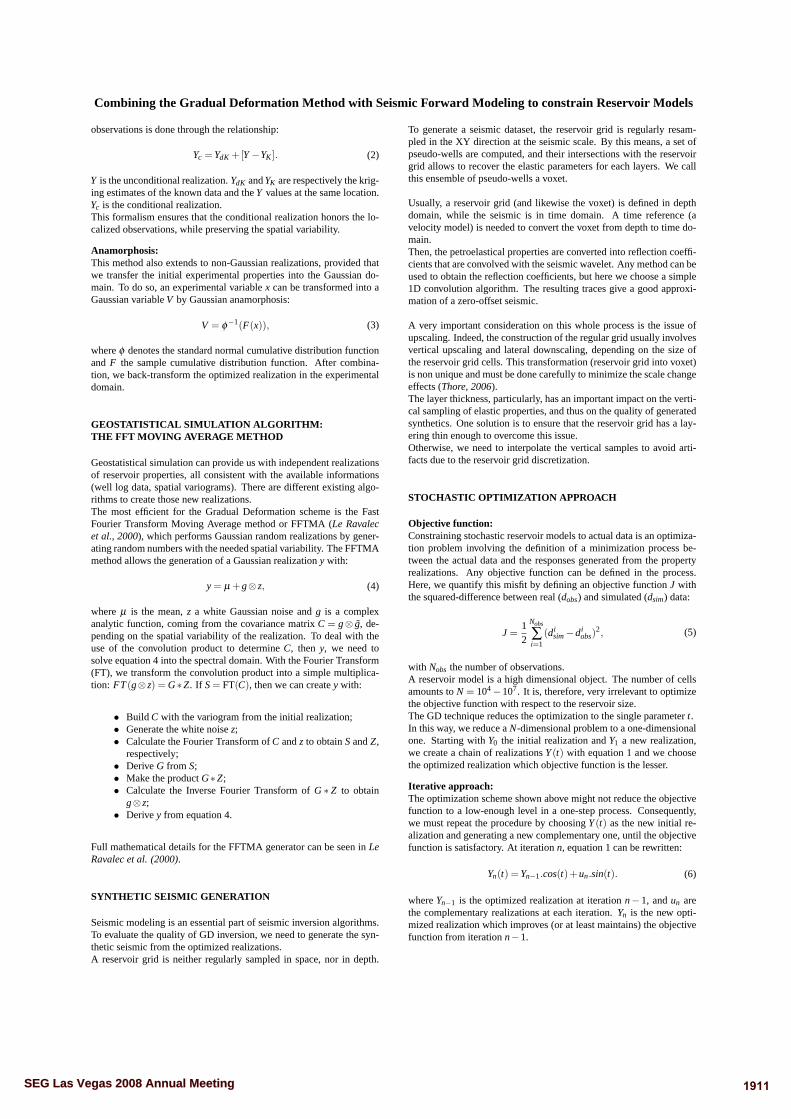
Combining the Gradual Deformation Method with Seismic Forward Modeling to constrain Reservoir Models
observations is done through the relationship:
Yc = YdK +[Y −YK ]. (2)
Y is the unconditional realization. YdK and YK are respectively the krig-ing estimates of the known data and the Y values at the same location.Yc is the conditional realization.This formalism ensures that the conditional realization honors the lo-calized observations, while preserving the spatial variability.
Anamorphosis:This method also extends to non-Gaussian realizations, provided thatwe transfer the initial experimental properties into the Gaussian do-main. To do so, an experimental variable x can be transformed into aGaussian variable V by Gaussian anamorphosis:
V = φ−1(F(x)), (3)
where φ denotes the standard normal cumulative distribution functionand F the sample cumulative distribution function. After combina-tion, we back-transform the optimized realization in the experimentaldomain.
GEOSTATISTICAL SIMULATION ALGORITHM:THE FFT MOVING AVERAGE METHOD
Geostatistical simulation can provide us with independent realizationsof reservoir properties, all consistent with the available informations(well log data, spatial variograms). There are different existing algo-rithms to create those new realizations.The most efficient for the Gradual Deformation scheme is the FastFourier Transform Moving Average method or FFTMA (Le Ravalecet al., 2000), which performs Gaussian random realizations by gener-ating random numbers with the needed spatial variability. The FFTMAmethod allows the generation of a Gaussian realization y with:
y = μ +g⊗ z, (4)
where μ is the mean, z a white Gaussian noise and g is a complexanalytic function, coming from the covariance matrix C = g⊗ g, de-pending on the spatial variability of the realization. To deal with theuse of the convolution product to determine C, then y, we need tosolve equation 4 into the spectral domain. With the Fourier Transform(FT), we transform the convolution product into a simple multiplica-tion: FT (g⊗ z) = G∗Z. If S = FT(C), then we can create y with:
• Build C with the variogram from the initial realization;• Generate the white noise z;• Calculate the Fourier Transform of C and z to obtain S and Z,
respectively;• Derive G from S;• Make the product G∗Z;• Calculate the Inverse Fourier Transform of G ∗ Z to obtain
g⊗ z;• Derive y from equation 4.
Full mathematical details for the FFTMA generator can be seen in LeRavalec et al. (2000).
SYNTHETIC SEISMIC GENERATION
Seismic modeling is an essential part of seismic inversion algorithms.To evaluate the quality of GD inversion, we need to generate the syn-thetic seismic from the optimized realizations.A reservoir grid is neither regularly sampled in space, nor in depth.
To generate a seismic dataset, the reservoir grid is regularly resam-pled in the XY direction at the seismic scale. By this means, a set ofpseudo-wells are computed, and their intersections with the reservoirgrid allows to recover the elastic parameters for each layers. We callthis ensemble of pseudo-wells a voxet.
Usually, a reservoir grid (and likewise the voxet) is defined in depthdomain, while the seismic is in time domain. A time reference (avelocity model) is needed to convert the voxet from depth to time do-main.Then, the petroelastical properties are converted into reflection coeffi-cients that are convolved with the seismic wavelet. Any method can beused to obtain the reflection coefficients, but here we choose a simple1D convolution algorithm. The resulting traces give a good approxi-mation of a zero-offset seismic.
A very important consideration on this whole process is the issue ofupscaling. Indeed, the construction of the regular grid usually involvesvertical upscaling and lateral downscaling, depending on the size ofthe reservoir grid cells. This transformation (reservoir grid into voxet)is non unique and must be done carefully to minimize the scale changeeffects (Thore, 2006).The layer thickness, particularly, has an important impact on the verti-cal sampling of elastic properties, and thus on the quality of generatedsynthetics. One solution is to ensure that the reservoir grid has a lay-ering thin enough to overcome this issue.Otherwise, we need to interpolate the vertical samples to avoid arti-facts due to the reservoir grid discretization.
STOCHASTIC OPTIMIZATION APPROACH
Objective function:Constraining stochastic reservoir models to actual data is an optimiza-tion problem involving the definition of a minimization process be-tween the actual data and the responses generated from the propertyrealizations. Any objective function can be defined in the process.Here, we quantify this misfit by defining an objective function J withthe squared-difference between real (dobs) and simulated (dsim) data:
J =12
Nobs
∑i=1
(disim−di
obs)2, (5)
with Nobs the number of observations.A reservoir model is a high dimensional object. The number of cellsamounts to N = 104−107. It is, therefore, very irrelevant to optimizethe objective function with respect to the reservoir size.The GD technique reduces the optimization to the single parameter t.In this way, we reduce a N-dimensional problem to a one-dimensionalone. Starting with Y0 the initial realization and Y1 a new realization,we create a chain of realizations Y (t) with equation 1 and we choosethe optimized realization which objective function is the lesser.
Iterative approach:The optimization scheme shown above might not reduce the objectivefunction to a low-enough level in a one-step process. Consequently,we must repeat the procedure by choosing Y (t) as the new initial re-alization and generating a new complementary one, until the objectivefunction is satisfactory. At iteration n, equation 1 can be rewritten:
Yn(t) = Yn−1.cos(t)+un.sin(t). (6)
where Yn−1 is the optimized realization at iteration n− 1, and un arethe complementary realizations at each iteration. Yn is the new opti-mized realization which improves (or at least maintains) the objectivefunction from iteration n−1.
1911SEG Las Vegas 2008 Annual Meeting
Main Menu
1911

Combining the Gradual Deformation Method with Seismic Forward Modeling to constrain Reservoir Models
EXAMPLE BASED ON A SYNTHETIC RESERVOIR CASE
We describe the use of GDM in the particular case of seismic inver-sion. Initial reservoir realizations are given as input to the GD Pro-cess. These realizations can be created by any means (smooth modelfrom Kriging of logs, stratigraphic model from geologic knowledge,etc . . . ). The basic statistics and spatial variability are extracted fromthese initial realizations. We can then create as much complementaryrealizations as wanted.Next, the GD Process is applied to generate optimized realizationswhich are then conditioned to well data by Kriging. If the initial real-izations are petrophysical properties, they are combined together witha rock physics model to obtain petroelastic properties. If the initialrealizations are petroelastic properties, we go ahead to the next step.We perform seismic forward modeling to obtain the seismic datasetsthat we compare to each other. The assessment of the objective func-tion enables either to change t, to begin a new iteration or to stop theprocess (see Figure 1).
Synthetic model description:We have a 3D reservoir model consisting of 26*26*113 = 76 388 cells,defined in the time domain (no time to depth conversion is required),with the following properties:
• ”True” P-velocity Vpreal and density ρreal , from which wecreate the ”actual” seismic dataset;
• Initial P-density Vpinit and density ρinit as input realizationsfor the process. Here, they were created from a supposed ge-ological knowledge (repartition of facies in the grid);
• P-velocity Vplog and density ρlog logs upscaled into the reser-voir grid to constrain the new realizations to the real proper-ties.
The process needs correlation lengths (given in number of cells) todefine the variogram of the complementary realizations. One for themaximum horizontal range for the x-direction of the reservoir model,Lx , and one for the y-direction, Ly. There is also a vertical range Lz,defined implicitly in the process, to assure that the realizations by lay-ers do not differ too much from each other. Here, we define Lx = 10cells, Ly = 20 cells and Lz = 2 layers.We also provide a wavelet for the generation of both actual and syn-thetic seismic datasets. The optimized realizations in the reservoir gridare exported in a Voxet. The ”actual” and synthetic datasets are mod-eled using a simple 1D convolution technique. Figure 2 shows thedifferent seismic datasets.
Figure 2: From left to right, seismic sections from initial and finalrealizations respectively, and ”actual” seismic section.
Results:We show in the figures hereafter the results for the gradual deformationinversion. A process of 250 iterations runs for about 5 hours. Figure2 shows how much the process change the initial synthetic section toobtain the final synthetic section. One can observe the non-seismic as-pect of the initial seismic.The objective function decreases by 69% from its initial value. Thisis illustrated on Figure 3, with the initial residuals (computed from theactual seismic and the initial synthetic sections) and the final residuals(between actual and final sections).Figure 4 shows the 51st layer in the reservoir model. The first row isthe P-velocity and the second one is the density. Again, one can ob-serve the evolution between the initial and the final property realiza-tions. We can also notice that the final properties recover the generalshape of the real properties (smoothed aspect).
DISCUSSION AND CONCLUSION
The Gradual Deformation Method is a parameterization technique thatallows to continuously perturb reservoir property realizations to solvean inverse problem. It takes into account scale change in the inversionprocess by simulating new realizations in a reservoir grid, while min-imizing an objective function between the actual seismic data and thesynthetic seismic datasets obtained from these realizations.It has been tested on a 3D synthetic reservoir model and shows im-provements of the reservoir realizations. The algorithm is not fullyoptimized but the run time is reasonable enough to consider using themethod on actual data.This feasibility test on seismic inversion directly in a reservoir modelwas done with the basic formulation for GDM. One of the first thingsto consider to optimize this algorithm is the improved GDM formula-tion (Hu et al, 2004), which consists in combining the initial realiza-tion with not one, but several complementary realizations. They alsodefined a gradient-oriented search to determine the best complemen-tary realizations for the next iteration and the associated deformationcoefficient t. Moreover, we can consider the use of parallel processing,by dividing the reservoir model in groups of layers with some layersin common between one group and the next. Our current researchesinclude these improvements.
ACKNOWLEDGMENTS
The authors would like to thank TOTAL for the release of this workfor publication.
1912SEG Las Vegas 2008 Annual Meeting
Main Menu
1912
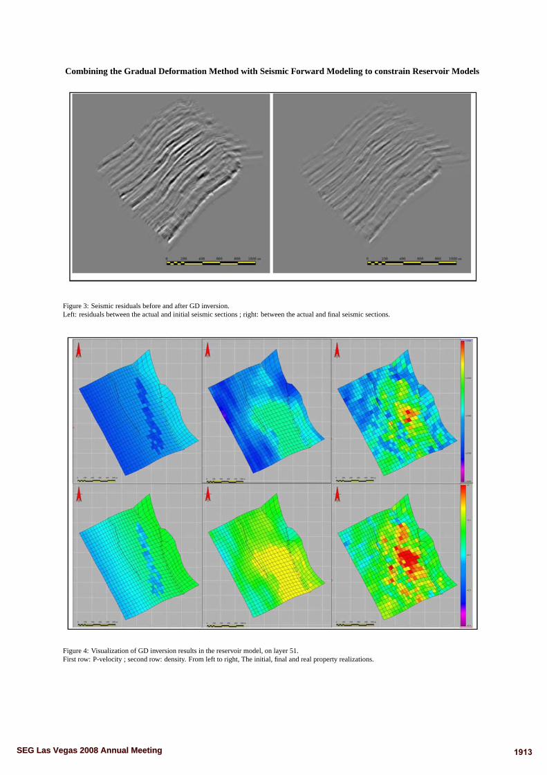
Combining the Gradual Deformation Method with Seismic Forward Modeling to constrain Reservoir Models
Figure 3: Seismic residuals before and after GD inversion.Left: residuals between the actual and initial seismic sections ; right: between the actual and final seismic sections.
Figure 4: Visualization of GD inversion results in the reservoir model, on layer 51.First row: P-velocity ; second row: density. From left to right, The initial, final and real property realizations.
1913SEG Las Vegas 2008 Annual Meeting
Main Menu
1913

EDITED REFERENCES Note: This reference list is a copy-edited version of the reference list submitted by the author. Reference lists for the 2008 SEG Technical Program Expanded Abstracts have been copy edited so that references provided with the online metadata for each paper will achieve a high degree of linking to cited sources that appear on the Web. REFERENCES Hu, L.-Y., 2000, Gradual deformation and iterative calibration of Gaussian-related stochastic models: Mathematical Geology, 32,
87–108. Hu, L.-Y., and M. Le Ravalec, 2004, An improved gradual deformation method for reconciling random and gradient searches in
stochastic optimizations: Mathematical Geology, 36, 703–719. Le Ravalec, M., B. Noetinger, and L.-Y. Hu, 2000, The FFT moving average (FFTMA) generator: An efficient numerical method
for generating and conditioning Gaussian simulations: Mathematical Geology, 32, 701–723. Thore, P., 2006, Accuracy and limitations in seismic modeling of reservoir: 76th Annual International Meeting, SEG, Expanded
Abtracts, 1674–1676.
1914SEG Las Vegas 2008 Annual Meeting
Main Menu
1914

Bibliographie
191

Bibliographie
Aki, K. and Richards, P. (1980). Quantitative Seismology : Theory and Methods. W. H.Freeman, New York.
Avseth, P., Mukerji, T., and Mavko, G. (2005). Quantitative Seismic Interpretation :Applying Rock Physics Tools to Reduce Interpretation Risk . Cambridge University Press.
Balz, O., Pivot, F., and Veeken, P. (1999). Reservoir characterization using neural networkscontrolled by petrophysical and seismic modeling. EAGE 61th Conference and Exhibition- Helsinki, Finland, 7 - 11 June 1999 .
Biot, M. A. (1956a). Theory of propagation of elastic waves in a �uid saturated poroussolid. i low frequency range. The Journal of the Acoustical Society of America, 28(2),168�178.
Biot, M. A. (1956b). Theory of propagation of elastic waves in a �uid saturated poroussolid. ii higher frequency range. Journal of the Acoustical Society of America, 28(2),179�191.
Bornard, R., Allo, F., Coleou, T., Freudenreich, Y., Caldwell, D. H., and Hamman, J. G.(2005). Petrophysical seismic inversion to determine more accurate and precise reservoirproperties. SPE Europec, Madrid, 13-16 June 2005 , (SPE94144).
Bosch, M., Zamora, M., and Utama, W. (2002). Lithology discrimination from physicalrock properties. Geophysics, 67(2), 573�581.
Breton, P., Modin, D., Duplantier, O., Thore, P., and Bredel, M. (2007). Seismic forwardmodeling for more representative reservoir model. EAGE 69th Conference and Exhibition- London, UK, 11 - 14 June 2007 .
Brown�eld, M. E. and Charpentier, R. R. (2006a). Geology and total petroleum systemsof the gulf of guinea province of west africa. U.S. Geological Survey Bulletin, 2207-C,32p. Available at http://pubs.usgs.gov/bul/2207/C/pdf/b2207c_508.pdf.
Brown�eld, M. E. and Charpentier, R. R. (2006b). Geology and total petroleum systems ofthe west-central coastal province, west africa. U.S. Geological Survey Bulletin, 2207-B,52p. Available at http://pubs.usgs.gov/bul/2207/B/pdf/b2207b_508.pdf.
Buland, A. and Omre, H. (2003). Bayesian linearized avo inversion. Geophysics, 68(1),185�198.
Caers, J. (2001). Geostatistical reservoir modeling using statistical pattern recognition.Journal of Petroleum Science and Engineering , 29(3), 177�188.
194 Bibliographie
Caers, J. and Zhang, T. (2002). Multiple-point geostatistics : a quantitative vehicle forintegrating geologic analogs into multiple reservoir models. In G. Grammer, editor,Integration of outcrop and modern analog data in reservoir models. European Associationof Geoscientists and Engineers.
Caers, J. F. (2007). Comparing the gradual deformation with the probability perturbationmethod for solving inverse problems. Mathematical Geology , 39(1), 27�52.
Cambois, G. (2000). Can p-wave avo be quantitative ? The Leading Edge, 19(11), 1246�1251.
Campbell, A., Fryer, A., and Wakeman, S. (2005). Vertical seismic pro�les, more than justa corridor stack. The Leading Edge, 24(7), 694�697.
Carcione, J. M., Hermanz, G. C., and ten Kroode, A. P. E. (2002). Seismic modeling.Geophysics, 67, 1304�1325.
Castagna, J. P., Batzle, M. L., and Eastwood, R. L. (1985). Relationships betweencompressionnal-wave ans shear-wave velocities in clastic silicate rocks. Geophysics, 50,571�581.
Castagna, J. P., Batzle, M. L., and Kan, T. K. (1993). Rock physics - the link bet-ween rock properties and avo response. In J. P. Castagna and M. M. Backus, edi-tors, O�set-dependant re�ectivity - Theory and practice of AVO analysis, pages 135�171.Soc.Expl.Geophys.
Cerveny, V. (2001). Seismic Ray Theory . Cambridge University Press.Chandra, M., Srivastava, A. K., Singh, V., Tiwary, D. N., and Painuly, P. K. (2003).Lithostratigraphic interpretation of seismic data for reservoir characterization. AAPGInternational Conference - Barcelona, Spain, 21 - 24 September 2003 .
Chen, H. and Castagna, J. P. (2000). Anisotropic e�ects on full and partial stacks. Geo-physics, 65(4), 1028�1031.
Chiles, J. and Del�ner, P. (1999). Geostatistics - Modeling spatial uncertainty . Wiley seriesin probability and statistics, New York, USA.
Cognot, R., Thore, P., and Haas, A. (1994). Tying seismic to well data using structuraluncertainties. SEG Technical Program Expanded Abstracts, 13(1), 494�497.
Coleou, T., Poupon, M., and Azbel, K. (2003). Interpreter's corner�unsupervised seismicfacies classi�cation : A review and comparison of techniques and implementation. TheLeading Edge, 22(10), 942�953.
Coleou, T., Formento, J.-L., Gram-Jensen, M., van Wijngaarden, A.-J., Haaland, A. N.,and Ona, R. (2006). Petrophysical seismic inversion applied to the troll �eld. SEGTechnical Program Expanded Abstracts, 25(1), 2107�2111.
Corredor, F., Shaw, J. H., and Bilotti, F. (2005). Structural styles in the deep-water foldand thrust belts of the niger delta. AAPG Bulletin, 89(6), 753�780.
deGroot, P., Campbell, A., Kavli, T., and Meynyk, D. (1993). Reservoir characterizationfrom 3d seismic data using neural networks and stochastic modelling techniques. EAGE55th Conference and Exhibition - Stavanger, Norway, June 1993 .

Bibliographie 195
deGroot, P. F. M., Bril, A. H., Florist, F. J., and Campbell, E. A. (1996). Monte carlosimulation of wells. Geophysics, 61(3), 631�638.
Doyen, P. M. (2007). Seismic reservoir characterization : an Earth modelling perspective.EAGE Publications BV.
Dubrule, O. (2003). Geostatistics for seismic data integration in Earth Models. EuropeanAssociation of Geoscientists and Engineers.
Dumay, J. and Fournier, F. (1988). Multivariate statistical analyses applied to seismicfacies recognition. Geophysics, 53(9), 1151�1159.
Duplantier, O., Hadj-Kacem, N., and Vittori, J. (2006). New strategies for seismic faciesupscaling to the reservoir grid scale. SPE Annual Technical Conference and Exhibition,San Antonio, Texas, (SPE101945).
Egreteau, A. (2005). Etude des variations de l'amplitude de la ré�ectivité du sous-sol aprèsimagerie sismique en profondeur . Ph.D. thesis, Ecole des Mines de Paris.
Enge, H. D., Buckley, S. J., Rotevant, A., and Howell, J. A. (2007). From outcrop toreservoir simulation model : Work�ow and procedures. Geosphere, 3(6), 469�490.
Escobar, I., Williamson, P., Cherrett, A., Doyen, P. M., Bornard, R., Moyen, R., andCrozat, T. (2006). Fast geostatistical stochastic inversion in a stratigraphic grid. SEGTechnical Program Expanded Abstracts, 25(1), 2067�2071.
Fang, J. H., Karr, C. L., and Stanley, D. A. (1992). Genetic algorithm and its applicationto petrophysics. (SPE26208).
Fournier, F. and Derain, J. F. (1992). Seismic data integration in reservoir simulationsthrough a multivariate statistical calibration approach. SEG Technical Program Expan-ded Abstracts, 11(1), 95�98.
Fournier, F. and Derain, J.-F. (1995). A statistical methodology for deriving reservoirproperties from seismic data. Geophysics, 60(5), 1437�1450.
Francis, A. M. (2002). Deterministic inversion : Overdue for retirement ? PETEX 2002Conference and Exhibition, London, UK .
Francis, A. M. (2005). Limitations of deterministic and advantages of stochastic seismicinversion. CSEG Recorder , pages 5�11.
Froidevaux, R. (1993). Probability �eld simulation. In A. Soares, editor, GeostatisticsTroia 1992 , volume 1, pages 73�84. Kluwer, New York.
Gardner, G. H. F., Gardner, L. W., and Gregory, A. R. (1974). Formation velocity anddensity - the diagnostic basics for stratigraphic traps. Geophysics, 39, 770�780.
Gassmann, F. (1951). Über die elastizität poröser medien. Vierteljahrsschrift der na-turforschenden geselishaft in Zürich, 96, 1�23. English traduction available at http://sepwww.stanford.edu/sep/berryman/PS/gassmann.pdf.
Gill, D., Shomrony, A., and Fligelman, H. (1993). Numerical zonation of log suites and logfacies recognition by multivariate clustering. AAPG Bulletin, 77, 1781�1791.
196 Bibliographie
Gnadesikan, R., Blash�eld, R. K., Breiman, L., Dunn, O. J., Friedman, J. H., Fu, K.,Hartigan, J., Kttenring, J. R., Lachenbruch, P. A., Olshen, R. A., and Rohlf, J. (1989).Discriminant analysis and clustering. Statistical Science, 4, 34�69.
Gomez, J. and Srivastava, R. (1990). Isim3d : an ansi-c tree-dimensional multiple indicatorfor conditional simulation. Computer and Geosciences, 16, 395�410.
Goovaerts, P. (1997). Geostatistics for natural resources evaluation. Applied GeostatisticsSeries, New York, USA.
Goovaerts, P. (2002). Geostatistical modeling of spatial uncertainty using p-�eld simulationwith conditional probability �elds. International Journal of Geographical InformationScience, 16, 167�178.
Hadj-Kacem, N. and Pivot, F. (2005). "crafty" techniques for populating géomodèles withseismic attributes data. EAGE 67th Conference and Exhibition - Madrid, Spain, 13 - 16June 2005 .
HadjKacem, N. (2006). Intégration des données sismiques pour une modélisation statiqueet dynamique plus réaliste des réservoirs. Ph.D. thesis, Ecole des Mines de Paris.
Himberg, J., Korpiaho, K., Mannila, H., Tikanmaki, J., and Toivonen, H. (2001). Timeseries segmentation for context recognition in mobile devices. International Conferenceon Data Mining (ICDM 2001) - San Jose, USA, 29 November - 2 December 2001 , pages203�210.
Holland, J. H. (1975). Adaptation in Natural and Arti�cial Systems : An IntroductoryAnalysis with Applications to Biology, Control, and Arti�cial Intelligence. The Universityof Michigan.
Hu, L.-Y. (2000). Gradual deformation and iterative calibration of gaussian-related sto-chastic models. Mathematical Geology , 31(1), 87�108.
Hu, L.-Y. and Ravalec-Dupin, M. L. (2004). An improved gradual deformation methodfor reconciling random and gradient searches in stochastic optimizations. MathematicalGeology , 36(6), 703�719.
Hu, L.-Y., Ravalec-Dupin, M. L., Blanc, G., Roggero, F., and Noetinger, B. (1999). Redu-cing uncertainties in production forecasts by constraining geological modeling to dynamicdata. Annual Technical Conference of the SPE, Huston, USA, (SPE56703).
Insalaco, E., Virgone, A., Courme, B., Gaillot, J., Kamali, M., Moallemi, A., Lotfpour, M.,and Monibi, S. (2006). Upper dalan member and kangan formation between the zagrosmountains and o�shore fars, iran : depositional system, biostratigraphy and stratigraphicarchitecture. GeoArabia, 11(2), 75�176.
Journel, A. G. and Ying, Z. (2001). The theoretical links between sequential gaussiansimulation, gaussian truncated simulation and probability �eld simulation. MathematicalGeology , 33(1), 31�40.
Julien, P., Pivot, F., Douillard, A., El-Ouair, Y., and Toinet, S. (2002). The importanceof pre-stack massive seismic modeling for avo calibration and seismic reservoir characte-rization. SEG Technical Program Expanded Abstracts, 21(1), 1731�1734.
Bibliographie 197
Kohonen, T. (1990). The self-organizing map. Proceedings of the IEEE , 78(9), 1465�1480.Krebes, E. (2004). Seismic forward modeling. CSEG Recorder , pages 28�39.Lecerf, D., Navion, S., and Boelle, J.-L. (2009). Azimuthal residual velocity analysis ino�set vector for waz imaging. 71st EAGE Conference and Exhibition - Amsterdam, TheNetherlands, 8 - 11 June 2009 .
Lecomte, I. and Pochon-Guerin, L. (2005). Simulated 2d/3d psdm images with a fast,robust, and �exible �t-based �ltering approach. SEG Technical Program Expanded Abs-tracts, 24(1), 1810�1813.
Li, Y. and Kareem, A. (1991). Simulation of multivariate non stationary random processesby �t. Journal of Engineering Mechanics, 117(5), 1037�1058.
Linari, V. (2004). A practical approach to well-seismic data calibration. The Leading Edge,23(8), 774�775.
Mavko, G., Mukerji, T., and Dvorkin, J. (2003). The Rock Physics Handbook : Tools forSeismic Analysis of Porous Media. Cambridge University Press.
Menezes, C. and Gosselin, O. (2006). From logs scale to reservoir scale : Upscaling of thepetroelastic model. Annual Conference and Exhibition of the EAGE, Vienna, Austria,(SPE100233).
Moyen, R. (2005). Paramétrisation 3D de l'espace en géologie sédimentaire : Le modèleGEOCHRON . Ph.D. thesis, Institut National Polytechnique de Lorraine, Ecole Natio-nale Supérieure de Géologie.
Mukerji, T., Jorstad, A., Avseth, P., Mavko, G., and Granli, J. R. (2001). Mapping li-thofacies and pore-�uid probabilities in a north sea reservoir : Seismic inversions andstatistical rock physics. Geophysics, 66(4), 988�1001.
Narasimhan, T. N. (1983). A note on volume-averaging. In G. F. Pinder, editor, Flowthrough porous media, pages 46�50. Computational Mechanics Publication.
Neau, A., Thore, P., and de Voogd, B. (2007). Structural uncertainty e�ects on reservoirgrid in�lling. SEG Technical Program Expanded Abstracts, 26(1), 1397�1401.
Neau, A., Thore, P., and de Voogd, B. (2008). Combining the gradual deformation methodwith seismic forward modeling to constrain reservoir models. SEG Technical ProgramExpanded Abstracts, 27(1), 1910�1914.
Nivlet, P., Lefebvre, F., and Piazza, J. (2007). 3d seismic constraint de�nition in deep-o�shore turbidite reservoir. Oil and Gas Science and Technology , 62(2), 249�264.
Pennington, W. D. (1997). Seismic petrophysics : An applied science for reservoir geophy-sics. The Leading Edge, 16, 241�244.
Pollastro, R. M. (2003). Total petroleum systems of the paleozoic and jurassic, greaterghawar uplift and adjoining provinces of central saudi arabia and northern arabian-persian gulf. U.S. Geological Survey Bulletin, 2202-H, 107p. Available at http://pubs.usgs.gov/bul/b2202-h/b2202-h.pdf.

198 Bibliographie
Poulton, M. M. (2002). Neural networks as an intelligence ampli�cation tool : A review ofapplications. Geophysics, 67(3), 979�993.
Ravalec-Dupin, M. L., Noetinger, B., and Hu, L.-Y. (2000). The �t moving average (�t-ma) generator : an e�cient numerical method for generating and conditioning gaussiansimulations. Mathematical Geology , 32(6), 701�723.
Ringrose, P. S. (2007). Myths and realities in upscaling reservoir data and models.(SPE106620).
Romero, C. and Carter, J. (2001). Using genetic algorithms for reservoir characterisation.Journal of Petroleum Science and Engineering , 31(2), 113�123.
Ruan, F. and McLaughlin, D. (1998). An e�cient multivariate random �eld generatorusing the fast fourier transform. Advances in water resources, 21, 385�399.
Saggaf, M. M., Toksöz, M. N., and Mustafa, H. M. (2003). Estimation of reservoir propertiesfrom seismic data by smooth neural networks. Geophysics, 68(6), 1969�1983.
Samson, P., Dubrule, O., and Euler, N. (1996). Quantifying the impact of structural uncer-tainties on gross rock volume estimates. European 3-D Reservoir Modelling Conference- Stavanger, Norway, 16 - 17 April 1996 , (SPE35535).
Sen, M. K. (2006). Seismic Inversion. Society of Petroleum Engineers, USA.Sen, M. K. and Sto�a, P. L. (1992). Genetic inversion of avo. The Leading Edge, 11(1),27�29.
Souche, L. (2005). Méthodes numériques pour la représentation des failles et des structuresgéologiques faillées. Ph.D. thesis, Institut National Polytechnique de Lorraine, EcoleNationale Supérieure de Géologie.
Srivastava, E. M. (1992). Reservoir characterization with probability �eld simulation.Annual Technical Conference of the SPE, Washington D.C., USA, (SPE24753), 927�938.
Sto�a, P. L. and Sen, M. K. (1991). Nonlinear multiparameter optimization using geneticalgorithms : Inversion of plane-wave seismograms. Geophysics, 56(11), 1794�1810.
Strebelle, S. (2000). Sequential simulation drawing structures from training images. Ph.D.thesis, Stanford University.
Strebelle, S., Payrazyan, K., and Caers, J. (2002). Modeling of a deepwater turbiditereservoir conditional to seismic data using multiple-point geostatistics. Annual TechnicalConference of the SPE, San Antonio, USA, (77425).
Thore, P., Shtuka, A., Lecour, M., Ait-Ettajer, T., and Cognot, R. (2002). Structuraluncertainties : Determination, management, and applications. Geophysics, 67(3), 840�852.
Thore, P., Morin, G., and Neau, A. (2008). A genetic algorithm for optimal blocking ofwell logs. EAGE 70th Conference and Exhibition - Rome, Italy, 9 - 12 June 2008 .
Tonn, R. (2002). Neural network seismic reservoir characterization in a heavy oil reservoir.The Leading Edge, 21(3), 309�312.

Bibliographie 199
Virieux, J. (1986). P-sv wave propagation in heterogeneous media : Velocity-stress �nite-di�erence method. Geophysics, 51(4), 889�901.
Virieux, J. and Farra, V. (1991). Ray tracing in 3-d complex isotropic media : An analysisof the problem. Geophysics, 56(12), 2057�2069.
Walden, A. T. (1991). Making avo sections more robust. Geophysical Prospecting , 39,915�942.
Walden, A. T. and White, R. E. (1984). On errors of �t and accuracy in matching syntheticseismograms and seismic traces. Geophysical Prospecting , 32, 871�891.
Wang, Z. Z. (2001). Fundamentals of seismic rock physics. Geophysics, 66, 398�412.White, R. and Simm, R. (2003). Good practice in well ties. First Break , 21(10), 75�83.Williamson, P., Cherrett, A., and Bornard, R. (2007). Geostatistical stochastic elasticinversion - an e�cient method for integrating seismic and well data constraints. EAGE69th Conference and Exhibition - London, UK, 11 - 14 June 2007 .
Yarus, J. M. and Chambers, R. L. (2006). Practical geostatistics, an armchair overview forpetroleum reservoir engineers. Journal of Petroleum Technology , pages 78�87.
Yilmaz, O. (2001). Seismic data analysis : Processing, Inversion, and Interpretation ofSeismic data. Investigations in Geophysics no.10 - 2nd Edition. Soc.Expl.Geophys.
Yin, Y. and Pillet, W. (2006). Seismic data preparation for improved elastic inversion ofangle stacks. SEG Technical Program Expanded Abstracts, 25(1), 2042�2046.
Ziolkowski, A., Underhill, J. R., and Johnston, R. G. K. (1998). Wavelets, well ties andthe search for subtle stratigraphic traps. Geophysics, 63(1), 297�313.
Caractérisation des réservoirs pétroliers par les données sismiques
avec l'aide de la géomodélisation
Résumé :La caractérisation sismique des réservoirs pétroliers nécessite l'intégration de plusieurs techniques(lithosismique, géomodélisation, géostatistique et pétrophysique). L'information sismique est d'abordutilisée pour décrire la structure des réservoirs car son utilisation pour la description des faciès nese fait pas sans di�cultés. L'objectif de cette thèse est d'apporter des outils nouveaux basés surl'utilisation de l'information sismique pour caractériser les réservoirs.Un premier travail a consisté à évaluer l'impact des incertitudes structurales et leurs conséquencesen terme de classi�cation de faciès. Ensuite, nous considérons la modélisation sismique comme aideà l'évaluation du modèle réservoir pour faire le lien entre les simulateurs et la réponse sismique duréservoir. Nous développons ensuite deux approches alternatives aux méthodes traditionnelles encaractérisation réservoir.La première utilise les déformations graduelles pour créer des réalisations de propriétés réservoirs.Ces propriétés sont à l'échelle réservoir, conditionnées aux puits, et respectent une fonction coûtbasée sur la comparaison des données sismiques réelles et synthétiques.La seconde méthode repose sur la classi�cation supervisée par réseaux de neurones pour analyser laforme des traces sismiques. Une première étape consiste à générer tous les modèles pétrophysiquesenvisageables et à les analyser par réseaux de neurones. Les neurones ainsi identi�és sont appliquésaux données réelles, pour trouver des relations pétrophysiques/sismiques identiques aux donnéesd'apprentissage.Tous les travaux sont validés sur des champs réels, choisis pour leurs particularités géologiques(lithologie du réservoir, complexité structurale).
Reservoir characterization based on seismic data with the help of
geomodeling methods
Abstract :Seismic characterization of hydrocarbon reservoirs is based on various techniques : lithoseismic,geomodeling, geostatistics, evolutionary algorithms, and petrophysics. Seismic information is �rstused for the description of the reservoir structure, but then its relationship with facies description isa di�cult task. The aim of this thesis is to develop new tools for seismic reservoir characterization.A �rst work has consisted in evaluating the impact of structural uncertainties on petroelastic in-version and its consequences in terms of facies classi�cation. Then, we consider seismic modelingas an aid to reservoir model evaluation. This modeling step will make the connection between thereservoir simulators (or geomodelers) and the seismic response of the reservoir.Then we develop two alternative approaches for petroelastic and petrophysical inversion. The �rstone uses the gradual deformation method to generate reservoir property realizations. This methodgenerates properties at the reservoir scale, conditioned by the wells, while respecting a cost functionbased on the comparison of actual and synthetic seismic data.The second method is based on supervised classi�cation principle and uses neural networks toanalyze the waveform of seismic traces. A �rst step is to generate a volume containing all possiblepetrophysical models for the concerned �eld. These models are analyzed by the neural networks.The neurons identi�ed are applied on the actual data to recognize similar petrophysical/seismicrelationships.All methods are tested and validated on actual reservoirs, chosen for their speci�c features (struc-tural complexity, reservoir lithology).