1

CASE STUDIES 1. ADVANCED SOLVER IS FASTER:

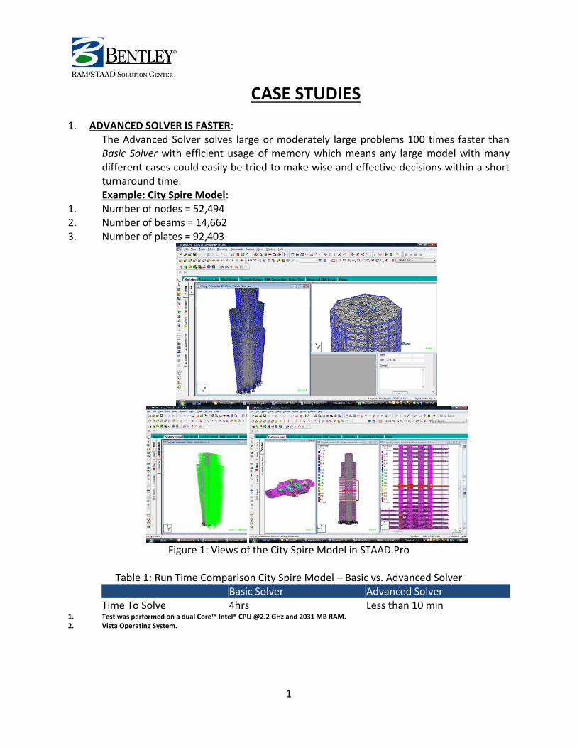
The Advanced Solver solves large or moderately large problems 100 times faster than Basic Solver with efficient usage of memory which means any large model with many different cases could easily be tried to make wise and effective decisions within a short turnaround time. Example: City Spire Model:

1. Number of nodes = 52,494 2. Number of beams = 14,662 3. Number of plates = 92,403

Figure 1: Views of the City Spire Model in STAAD.Pro

Table 1: Run Time Comparison City Spire Model – Basic vs. Advanced Solver

Basic Solver Advanced Solver Time To Solve 4hrs Less than 10 min

1. Test was performed on a dual Core™ Intel® CPU @2.2 GHz and 2031 MB RAM. 2. Vista Operating System.

2

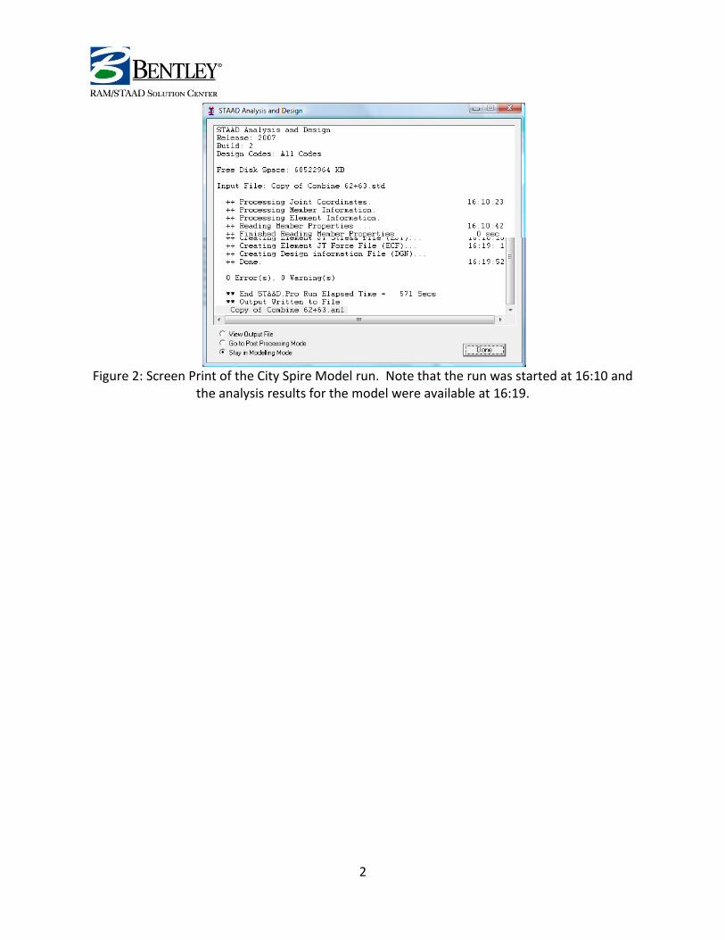
Figure 2: Screen Print of the City Spire Model run. Note that the run was started at 16:10 and

the analysis results for the model were available at 16:19.

3

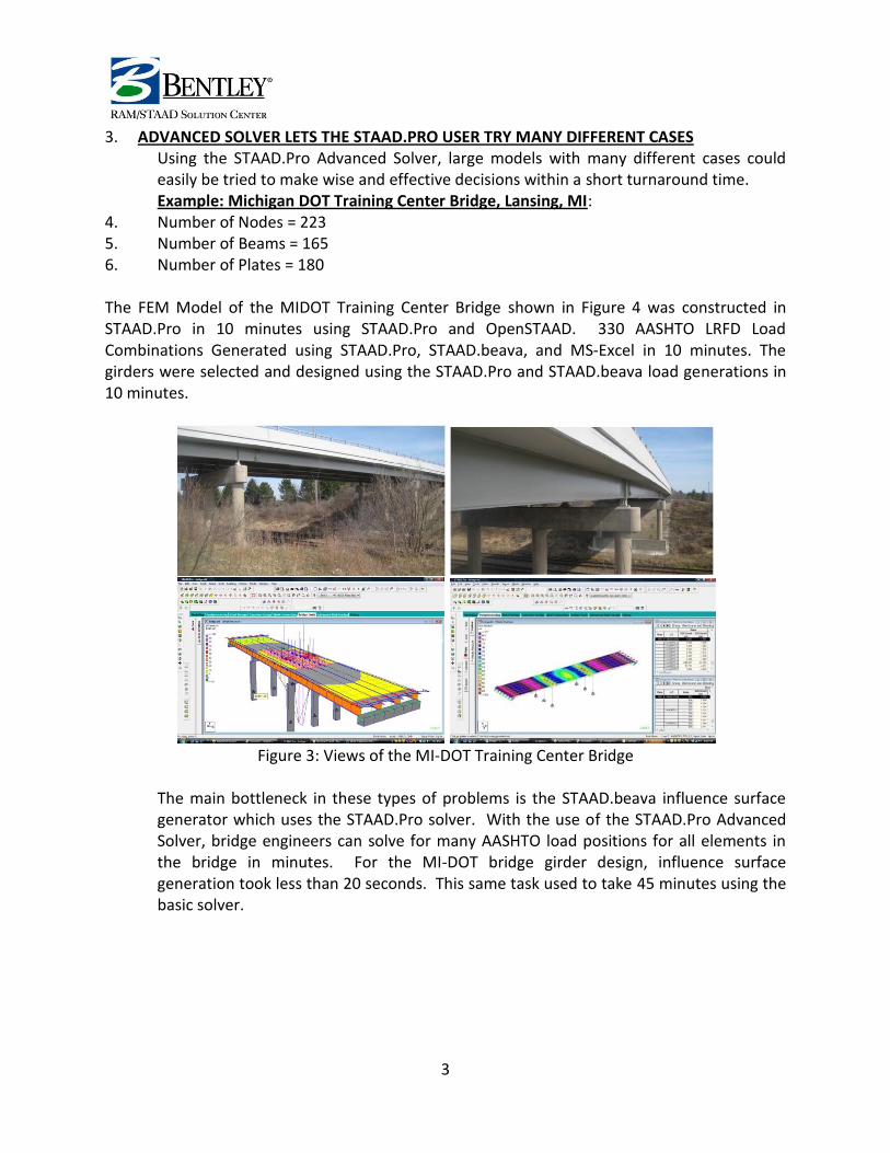
3. ADVANCED SOLVER LETS THE STAAD.PRO USER TRY MANY DIFFERENT CASES Using the STAAD.Pro Advanced Solver, large models with many different cases could easily be tried to make wise and effective decisions within a short turnaround time. Example: Michigan DOT Training Center Bridge, Lansing, MI:

4. Number of Nodes = 223 5. Number of Beams = 165 6. Number of Plates = 180 The FEM Model of the MIDOT Training Center Bridge shown in Figure 4 was constructed in STAAD.Pro in 10 minutes using STAAD.Pro and OpenSTAAD. 330 AASHTO LRFD Load Combinations Generated using STAAD.Pro, STAAD.beava, and MS‐Excel in 10 minutes. The girders were selected and designed using the STAAD.Pro and STAAD.beava load generations in 10 minutes.

Figure 3: Views of the MI-DOT Training Center Bridge

The main bottleneck in these types of problems is the STAAD.beava influence surface generator which uses the STAAD.Pro solver. With the use of the STAAD.Pro Advanced Solver, bridge engineers can solve for many AASHTO load positions for all elements in the bridge in minutes. For the MI-DOT bridge girder design, influence surface generation took less than 20 seconds. This same task used to take 45 minutes using the basic solver.

4

Table 2: Run Time Comparison MI-DOT Bridge – Basic vs. Advanced Solver Basic Solver Advanced Solver Time To Solve 45min Less than 20 seconds

1. Test was performed on a dual Core™ Intel® CPU @2.2 GHz and 2031 MB RAM. 2. Vista Operating System.

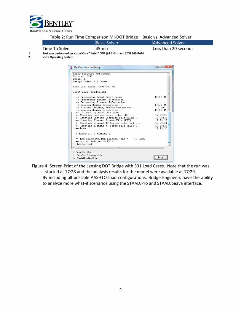
Figure 4: Screen Print of the Lansing DOT Bridge with 331 Load Cases. Note that the run was

started at 17:28 and the analysis results for the model were available at 17:29. By including all possible AASHTO load configurations, Bridge Engineers have the ability to analyze more what-if scenarios using the STAAD.Pro and STAAD.beava interface.

5

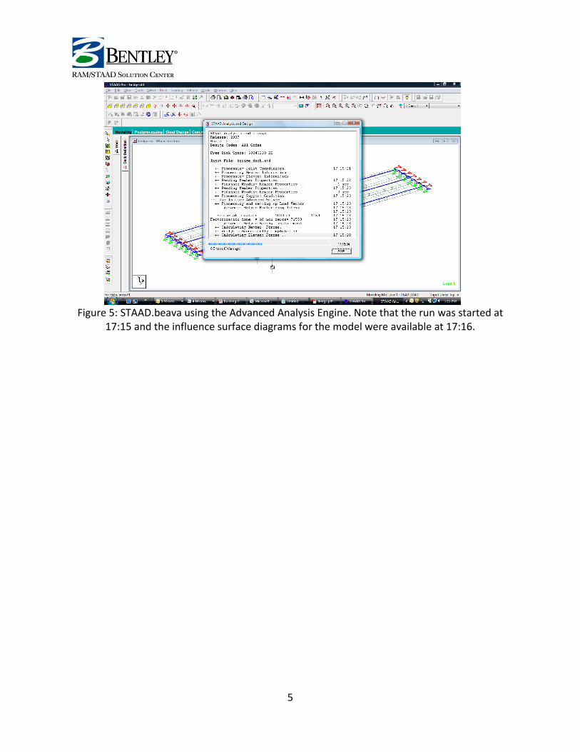
Figure 5: STAAD.beava using the Advanced Analysis Engine. Note that the run was started at

17:15 and the influence surface diagrams for the model were available at 17:16.

6

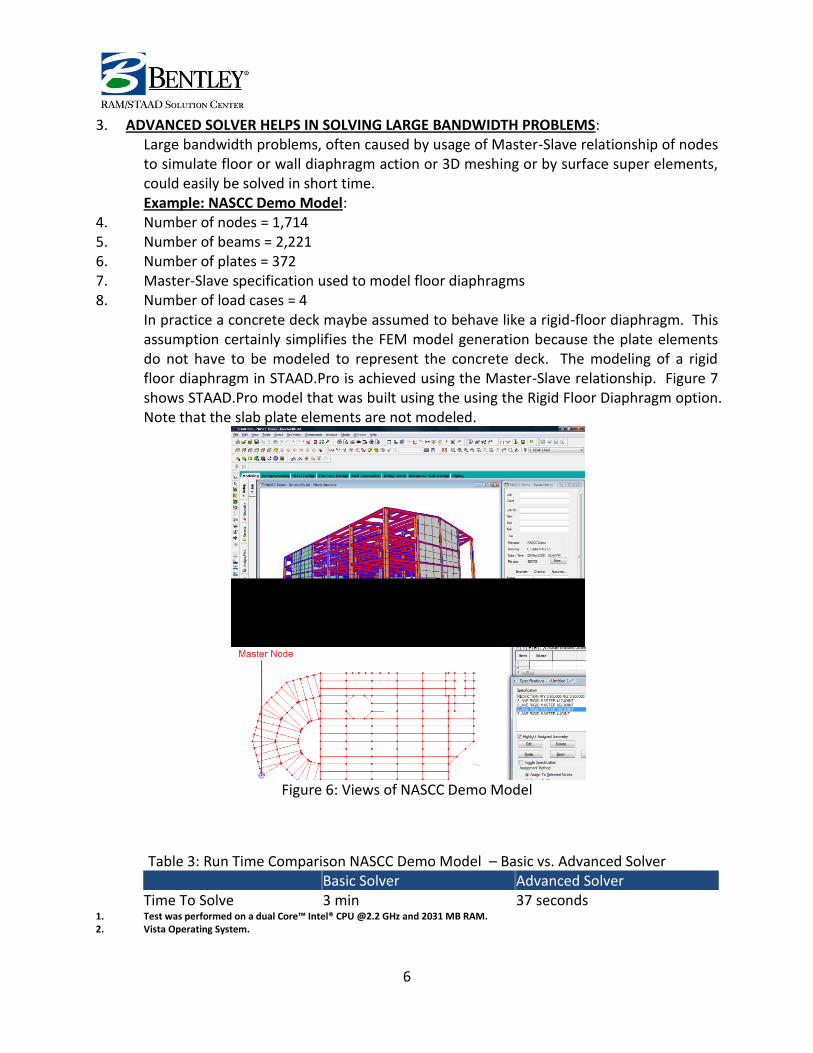
3. ADVANCED SOLVER HELPS IN SOLVING LARGE BANDWIDTH PROBLEMS: Large bandwidth problems, often caused by usage of Master-Slave relationship of nodes to simulate floor or wall diaphragm action or 3D meshing or by surface super elements, could easily be solved in short time. Example: NASCC Demo Model:

4. Number of nodes = 1,714 5. Number of beams = 2,221 6. Number of plates = 372 7. Master-Slave specification used to model floor diaphragms 8. Number of load cases = 4

In practice a concrete deck maybe assumed to behave like a rigid-floor diaphragm. This assumption certainly simplifies the FEM model generation because the plate elements do not have to be modeled to represent the concrete deck. The modeling of a rigid floor diaphragm in STAAD.Pro is achieved using the Master-Slave relationship. Figure 7 shows STAAD.Pro model that was built using the using the Rigid Floor Diaphragm option. Note that the slab plate elements are not modeled.

Figure 6: Views of NASCC Demo Model

Table 3: Run Time Comparison NASCC Demo Model – Basic vs. Advanced Solver Basic Solver Advanced Solver Time To Solve 3 min 37 seconds

1. Test was performed on a dual Core™ Intel® CPU @2.2 GHz and 2031 MB RAM. 2. Vista Operating System.

7

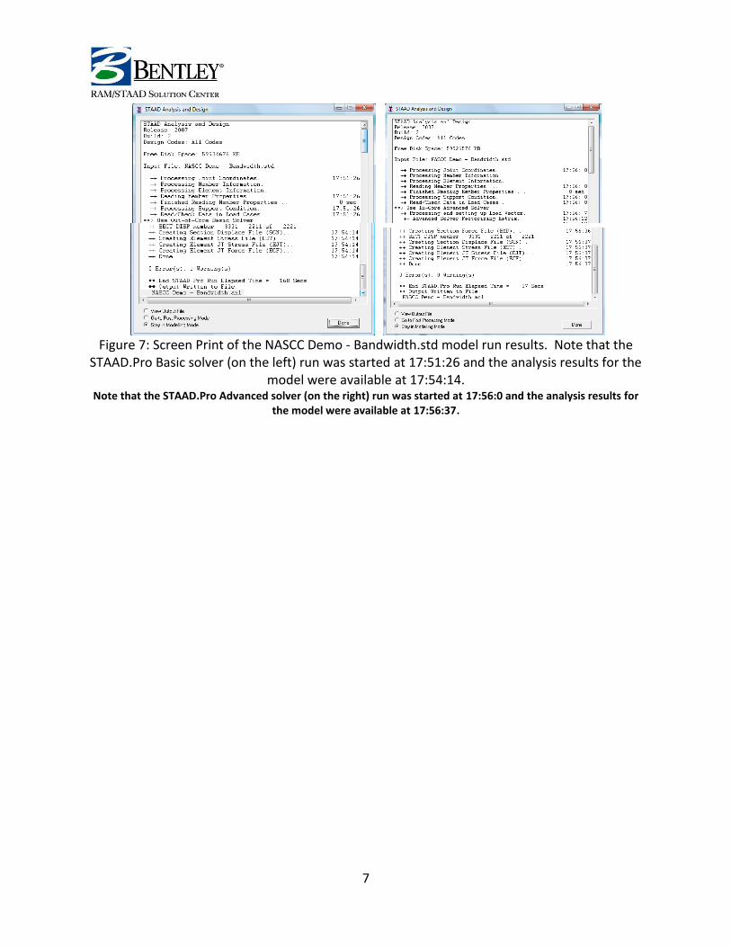
Figure 7: Screen Print of the NASCC Demo - Bandwidth.std model run results. Note that the

STAAD.Pro Basic solver (on the left) run was started at 17:51:26 and the analysis results for the model were available at 17:54:14.

Note that the STAAD.Pro Advanced solver (on the right) run was started at 17:56:0 and the analysis results for the model were available at 17:56:37.

8

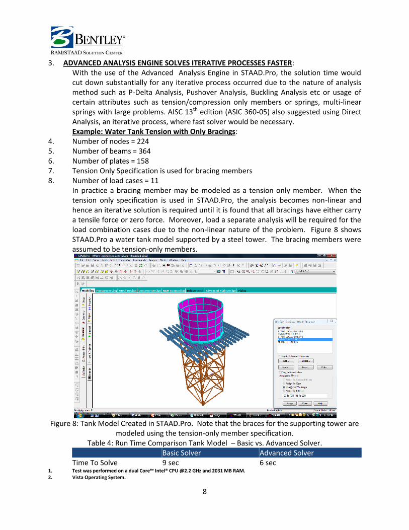
3. ADVANCED ANALYSIS ENGINE SOLVES ITERATIVE PROCESSES FASTER: With the use of the Advanced Analysis Engine in STAAD.Pro, the solution time would cut down substantially for any iterative process occurred due to the nature of analysis method such as P-Delta Analysis, Pushover Analysis, Buckling Analysis etc or usage of certain attributes such as tension/compression only members or springs, multi-linear springs with large problems. AISC 13th edition (ASIC 360-05) also suggested using Direct Analysis, an iterative process, where fast solver would be necessary. Example: Water Tank Tension with Only Bracings:

4. Number of nodes = 224 5. Number of beams = 364 6. Number of plates = 158 7. Tension Only Specification is used for bracing members 8. Number of load cases = 11

In practice a bracing member may be modeled as a tension only member. When the tension only specification is used in STAAD.Pro, the analysis becomes non-linear and hence an iterative solution is required until it is found that all bracings have either carry a tensile force or zero force. Moreover, load a separate analysis will be required for the load combination cases due to the non-linear nature of the problem. Figure 8 shows STAAD.Pro a water tank model supported by a steel tower. The bracing members were assumed to be tension-only members.

Figure 8: Tank Model Created in STAAD.Pro. Note that the braces for the supporting tower are

modeled using the tension-only member specification. Table 4: Run Time Comparison Tank Model – Basic vs. Advanced Solver.

Basic Solver Advanced Solver Time To Solve 9 sec 6 sec

1. Test was performed on a dual Core™ Intel® CPU @2.2 GHz and 2031 MB RAM. 2. Vista Operating System.

9

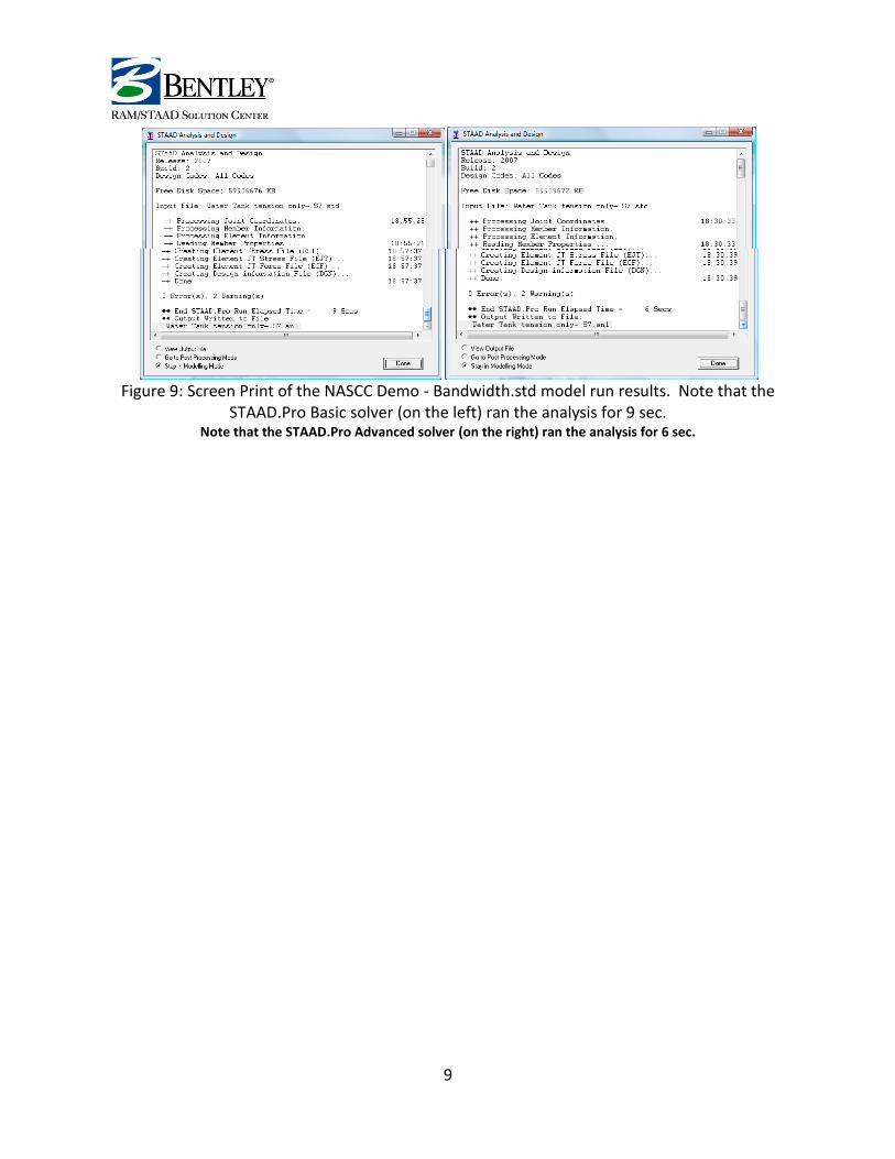
Figure 9: Screen Print of the NASCC Demo - Bandwidth.std model run results. Note that the

STAAD.Pro Basic solver (on the left) ran the analysis for 9 sec. Note that the STAAD.Pro Advanced solver (on the right) ran the analysis for 6 sec.

10

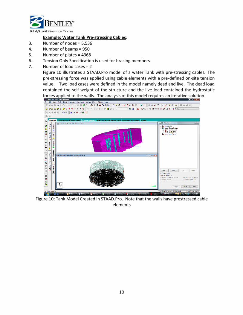
Example: Water Tank Pre-stressing Cables: 3. Number of nodes = 5,536 4. Number of beams = 950 5. Number of plates = 4368 6. Tension Only Specification is used for bracing members 7. Number of load cases = 2

Figure 10 illustrates a STAAD.Pro model of a water Tank with pre-stressing cables. The pre-stressing force was applied using cable elements with a pre-defined on-site tension value. Two load cases were defined in the model namely dead and live. The dead load contained the self-weight of the structure and the live load contained the hydrostatic forces applied to the walls. The analysis of this model requires an iterative solution.

Figure 10: Tank Model Created in STAAD.Pro. Note that the walls have prestressed cable

elements

11

Table 5: Run Time Comparison Water Tank with Pre-stressing Cables Model – Basic vs. Advanced Solver

Basic Solver Advanced Solver Time To Solve 235 sec 14 sec

1. Test was performed on a dual Core™ Intel® CPU @2.2 GHz and 2031 MB RAM. 2. Vista Operating System.

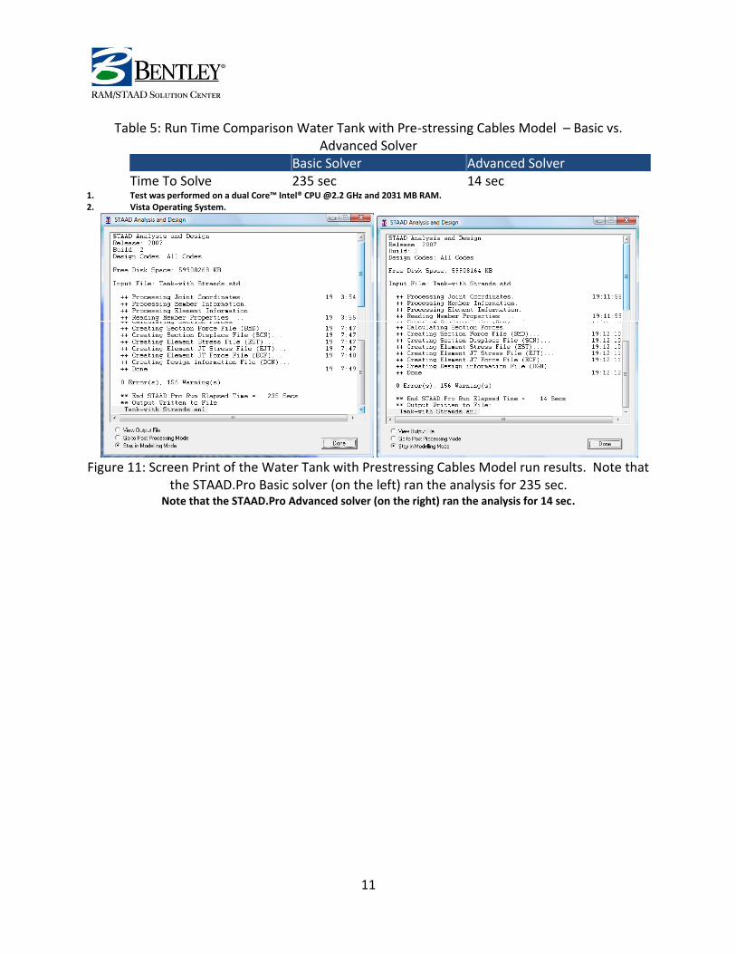
Figure 11: Screen Print of the Water Tank with Prestressing Cables Model run results. Note that

the STAAD.Pro Basic solver (on the left) ran the analysis for 235 sec. Note that the STAAD.Pro Advanced solver (on the right) ran the analysis for 14 sec.

12

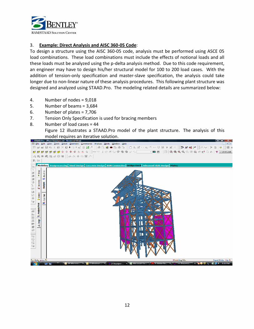
3. Example: Direct Analysis and AISC 360-05 Code: To design a structure using the AISC 360-05 code, analysis must be performed using ASCE 05 load combinations. These load combinations must include the effects of notional loads and all these loads must be analyzed using the p-delta analysis method. Due to this code requirement, an engineer may have to design his/her structural model for 100 to 200 load cases. With the addition of tension-only specification and master-slave specification, the analysis could take longer due to non-linear nature of these analysis procedures. This following plant structure was designed and analyzed using STAAD.Pro. The modeling related details are summarized below: 4. Number of nodes = 9,018 5. Number of beams = 3,684 6. Number of plates = 7,706 7. Tension Only Specification is used for bracing members 8. Number of load cases = 44

Figure 12 illustrates a STAAD.Pro model of the plant structure. The analysis of this model requires an iterative solution.

13

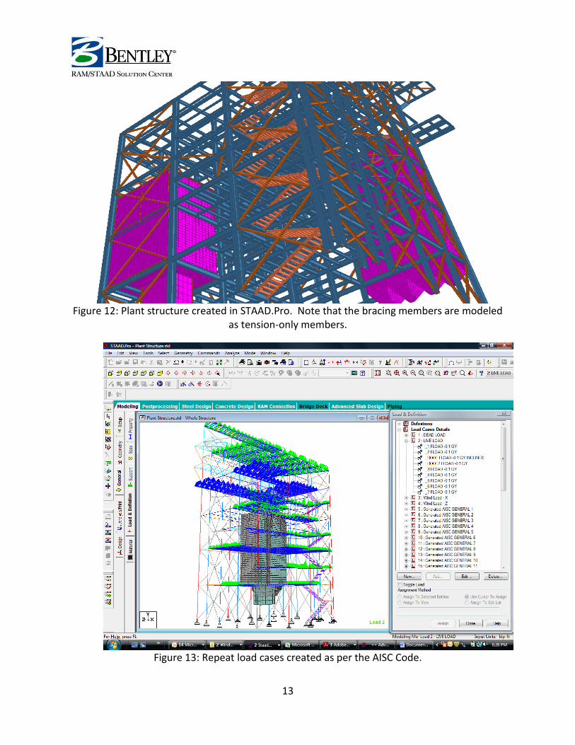
Figure 12: Plant structure created in STAAD.Pro. Note that the bracing members are modeled

as tension-only members.

Figure 13: Repeat load cases created as per the AISC Code.

14

Table 6: Run Time Comparison Plant Structure Model – Basic vs. Advanced Solver Basic Solver Advanced Solver Time To Solve More than 2 days (User

aborted) 20 min

9. Test was performed on a dual Core™ Intel® CPU @2.2 GHz and 2031 MB RAM. 10. Vista Operating System.

15

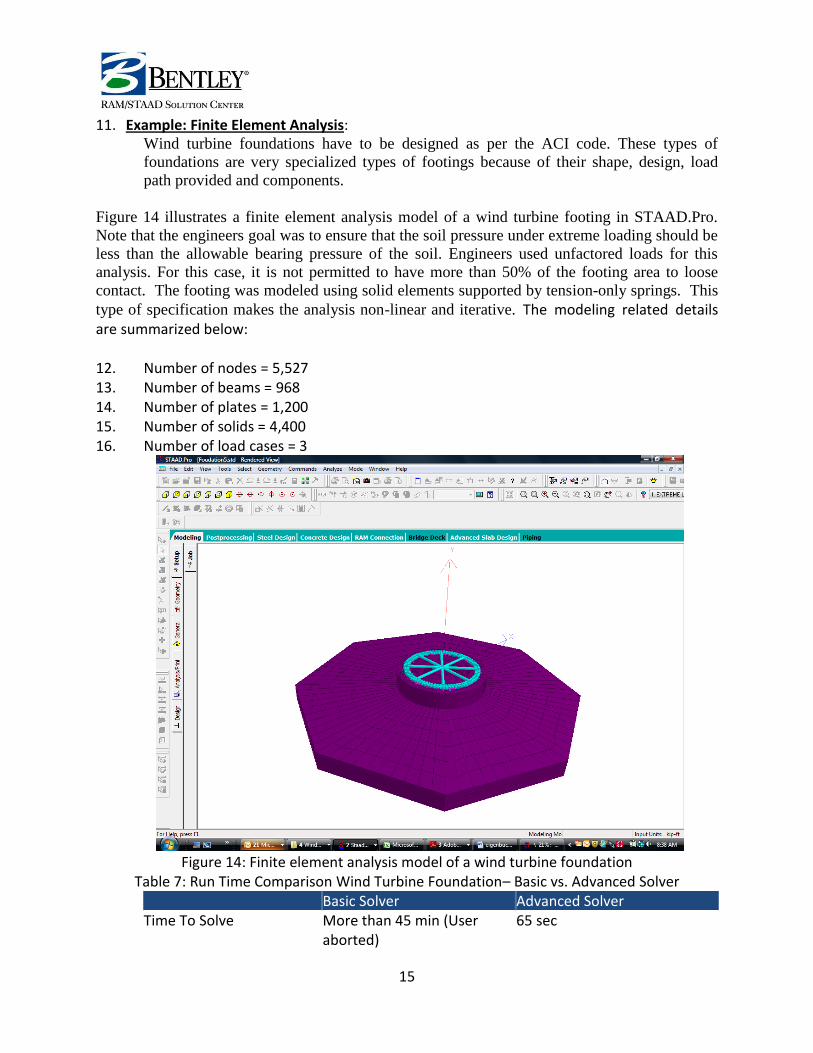
11. Example: Finite Element Analysis: Wind turbine foundations have to be designed as per the ACI code. These types of

foundations are very specialized types of footings because of their shape, design, load

path provided and components.

Figure 14 illustrates a finite element analysis model of a wind turbine footing in STAAD.Pro.

Note that the engineers goal was to ensure that the soil pressure under extreme loading should be

less than the allowable bearing pressure of the soil. Engineers used unfactored loads for this

analysis. For this case, it is not permitted to have more than 50% of the footing area to loose

contact. The footing was modeled using solid elements supported by tension-only springs. This

type of specification makes the analysis non-linear and iterative. The modeling related details are summarized below: 12. Number of nodes = 5,527 13. Number of beams = 968 14. Number of plates = 1,200 15. Number of solids = 4,400 16. Number of load cases = 3

Figure 14: Finite element analysis model of a wind turbine foundation

Table 7: Run Time Comparison Wind Turbine Foundation– Basic vs. Advanced Solver Basic Solver Advanced Solver Time To Solve More than 45 min (User

aborted) 65 sec

16

1. Test was performed on a dual Core™ Intel® CPU @2.2 GHz and 2031 MB RAM. 2. Vista Operating System.

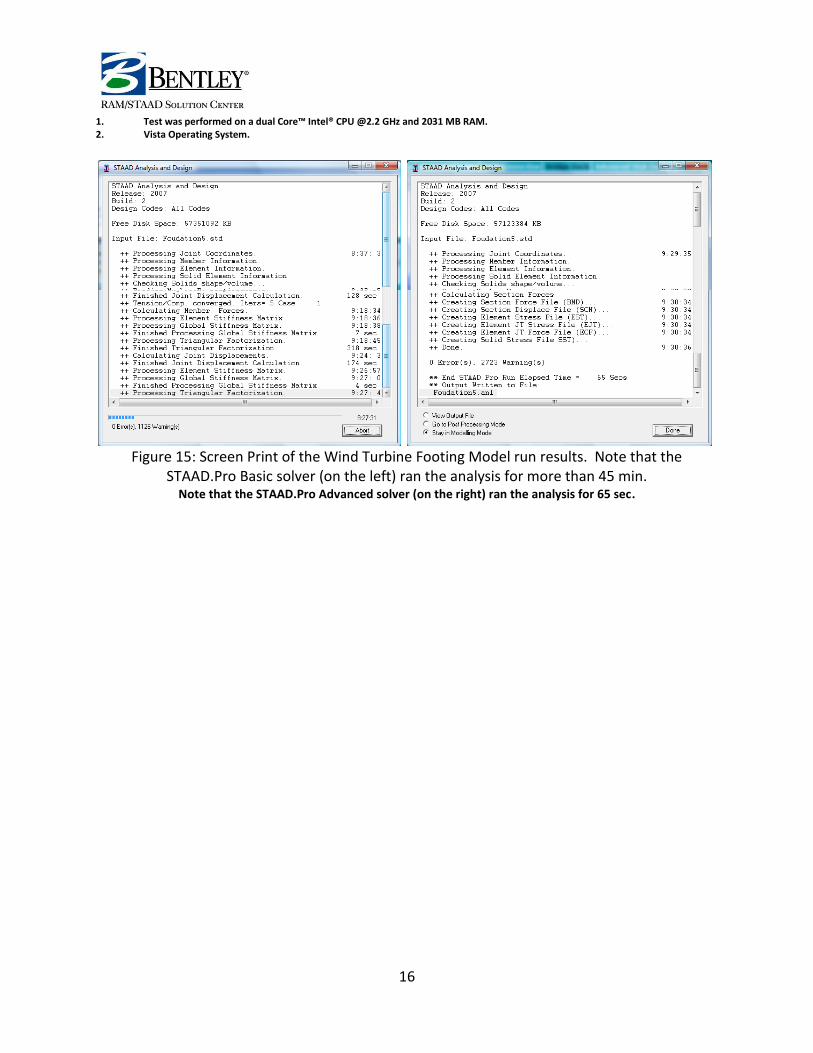
Figure 15: Screen Print of the Wind Turbine Footing Model run results. Note that the

STAAD.Pro Basic solver (on the left) ran the analysis for more than 45 min. Note that the STAAD.Pro Advanced solver (on the right) ran the analysis for 65 sec.

17

REQUIREMENT STUDY

Steady State Analysis:

A structure [subjected only to harmonic loading, all at a given forcing frequency and with non-

zero damping] will reach a steady state of vibration that will repeat every forcing cycle. This

steady state response can be computed without calculating the transient time history response

prior to the steady state condition.

Ground motion or a joint force distribution may be specified. Each global direction may be at a

different phase angle.

Output frequency points are selected automatically for modal frequencies and for a set number of

frequencies between modal frequencies. There is an option to change the number of points

between frequencies and an option to add frequencies to the list of output frequencies.

There are various instances in which this type of analysis maybe used. Some examples include:

1. Effect of a harmonic loading on a steel frame 2. Effect of a printing press on a steel frame 3. Turbine foundation or any machine supporting structure 4. Ground motion

18

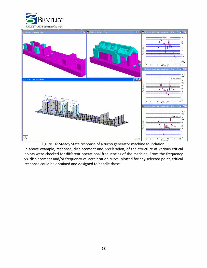
Figure 16: Steady State response of a turbo generator machine foundation.

In above example, response, displacement and acceleration, of the structure at various critical points were checked for different operational frequencies of the machine. From the frequency vs. displacement and/or frequency vs. acceleration curve, plotted for any selected point, critical response could be obtained and designed to handle these.

19

Eigen Buckling Analysis – Small and Large P-Delta effect – Buckling Modes

and Factors:

Eigen Buckling Analysis or classical Euler buckling analysis in STAAD.Pro will allow the users

to predict theoretical buckling strength of an ideal elastic structure. This feature computes

structural eigen values for a given system loading and constraints. By including the command

PERFORM BUCKLING ANALYSIS, the program will perform a P-Delta analysis including Kg

Stiffening (geometric stiffness of members & plates) due to large & small P-Delta effects. If a

non-singular stiffness matrix can be created, then buckling has not occurred.

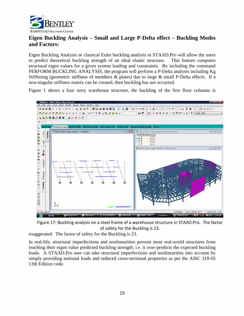
Figure 1 shows a four story warehouse structure, the buckling of the first floor columns is

exaggerated. The factor of safety for the Buckling is 23.

In real-life, structural imperfections and nonlinearities prevent most real-world structures from

reaching their eigen value predicted buckling strength; i.e. it over-predicts the expected buckling

loads. A STAAD.Pro user can take structural imperfections and nonlinearities into account by

simply providing notional loads and reduced cross-sectional properties as per the AISC 318-05

13th Edition code.

Figure 17: Buckling analysis on a steel frame of a warehouse structure in STAAD.Pro. The factor of safety for the Buckling is 23.