Embed Size (px)
Citation preview
Catalogue of Spacetimes
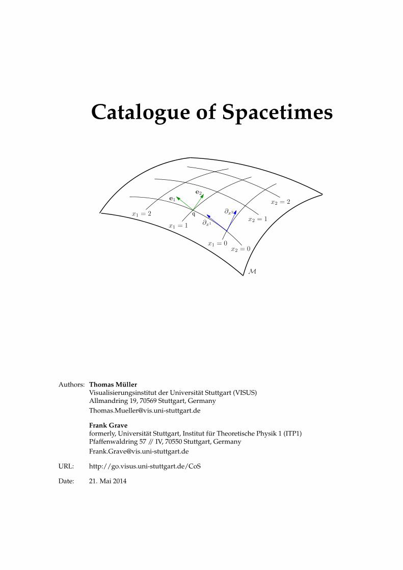
q
x1 = 0
x1 = 1
x1 = 2
x2 = 0
x2 = 1
x2 = 2
∂x2
∂x1
e2e1
M
Authors: Thomas MüllerVisualisierungsinstitut der Universität Stuttgart (VISUS)Allmandring 19, 70569 Stuttgart, [email protected]
Frank Graveformerly, Universität Stuttgart, Institut für Theoretische Physik 1 (ITP1)Pfaffenwaldring 57 // IV, 70550 Stuttgart, [email protected]
URL: http://go.visus.uni-stuttgart.de/CoS
Date: 21. Mai 2014
Co-authors
Andreas Lemmer, formerly, Institut für Theoretische Physik 1 (ITP1), Universität StuttgartAlcubierre Warp
Sebastian Boblest, Institut für Theoretische Physik 1 (ITP1), Universität StuttgartdeSitter, Friedmann-Robertson-Walker
Felix Beslmeisl, Institut für Theoretische Physik 1 (ITP1), Universität StuttgartPetrov-Type D
Heiko Munz, Institut für Theoretische Physik 1 (ITP1), Universität StuttgartBessel and plane wave
Andreas Wünsch, Institut für Theoretische Physik 1 (ITP1), Universität StuttgartMajumdar-Papapetrou, extreme Reissner-Nordstrøm dihole, energy momentum tensor
Many thanks to all that have reported bug fixes or added metric descriptions.
Contents
1 Introduction and Notation 11.1 Notation . . . . . . . . . . . . . . . . . . . . . . . . . . . . . . . . . . . . . . . . . . . . . . . 11.2 General remarks . . . . . . . . . . . . . . . . . . . . . . . . . . . . . . . . . . . . . . . . . . . 11.3 Basic objects of a metric . . . . . . . . . . . . . . . . . . . . . . . . . . . . . . . . . . . . . . 21.4 Natural local tetrad and initial conditions for geodesics . . . . . . . . . . . . . . . . . . . . 3
1.4.1 Orthonormality condition . . . . . . . . . . . . . . . . . . . . . . . . . . . . . . . . . 31.4.2 Tetrad transformations . . . . . . . . . . . . . . . . . . . . . . . . . . . . . . . . . . . 41.4.3 Ricci rotation-, connection-, and structure coefficients . . . . . . . . . . . . . . . . . 41.4.4 Riemann-, Ricci-, and Weyl-tensor with respect to a local tetrad . . . . . . . . . . . 41.4.5 Null or timelike directions . . . . . . . . . . . . . . . . . . . . . . . . . . . . . . . . . 51.4.6 Local tetrad for diagonal metrics . . . . . . . . . . . . . . . . . . . . . . . . . . . . . 51.4.7 Local tetrad for stationary axisymmetric spacetimes . . . . . . . . . . . . . . . . . . 5
1.5 Newman-Penrose tetrad and spin-coefficients . . . . . . . . . . . . . . . . . . . . . . . . . . 61.6 Coordinate relations . . . . . . . . . . . . . . . . . . . . . . . . . . . . . . . . . . . . . . . . 7
1.6.1 Spherical and Cartesian coordinates . . . . . . . . . . . . . . . . . . . . . . . . . . . 71.6.2 Cylindrical and Cartesian coordinates . . . . . . . . . . . . . . . . . . . . . . . . . . 7
1.7 Embedding diagram . . . . . . . . . . . . . . . . . . . . . . . . . . . . . . . . . . . . . . . . 81.8 Equations of motion and transport equations . . . . . . . . . . . . . . . . . . . . . . . . . . 9
1.8.1 Geodesic equation . . . . . . . . . . . . . . . . . . . . . . . . . . . . . . . . . . . . . 91.8.2 Fermi-Walker transport . . . . . . . . . . . . . . . . . . . . . . . . . . . . . . . . . . 91.8.3 Parallel transport . . . . . . . . . . . . . . . . . . . . . . . . . . . . . . . . . . . . . . 91.8.4 Euler-Lagrange formalism . . . . . . . . . . . . . . . . . . . . . . . . . . . . . . . . . 91.8.5 Hamilton formalism . . . . . . . . . . . . . . . . . . . . . . . . . . . . . . . . . . . . 10
1.9 Special topics . . . . . . . . . . . . . . . . . . . . . . . . . . . . . . . . . . . . . . . . . . . . 101.9.1 Timelike circular geodesics . . . . . . . . . . . . . . . . . . . . . . . . . . . . . . . . 10
1.10 Units . . . . . . . . . . . . . . . . . . . . . . . . . . . . . . . . . . . . . . . . . . . . . . . . . 101.11 Energy momentum tensor . . . . . . . . . . . . . . . . . . . . . . . . . . . . . . . . . . . . . 11
1.11.1 Energy conditions . . . . . . . . . . . . . . . . . . . . . . . . . . . . . . . . . . . . . 111.11.2 Examples for energy momentum tensors . . . . . . . . . . . . . . . . . . . . . . . . 11
1.12 Tools . . . . . . . . . . . . . . . . . . . . . . . . . . . . . . . . . . . . . . . . . . . . . . . . . 131.12.1 Maple/GRTensorII . . . . . . . . . . . . . . . . . . . . . . . . . . . . . . . . . . . . . 131.12.2 Mathematica . . . . . . . . . . . . . . . . . . . . . . . . . . . . . . . . . . . . . . . . 131.12.3 Maxima . . . . . . . . . . . . . . . . . . . . . . . . . . . . . . . . . . . . . . . . . . . 151.12.4 Sympy . . . . . . . . . . . . . . . . . . . . . . . . . . . . . . . . . . . . . . . . . . . . 16
2 Spacetimes 192.1 Minkowski . . . . . . . . . . . . . . . . . . . . . . . . . . . . . . . . . . . . . . . . . . . . . . 19
2.1.1 Cartesian coordinates . . . . . . . . . . . . . . . . . . . . . . . . . . . . . . . . . . . 192.1.2 Cylindrical coordinates . . . . . . . . . . . . . . . . . . . . . . . . . . . . . . . . . . 192.1.3 Spherical coordinates . . . . . . . . . . . . . . . . . . . . . . . . . . . . . . . . . . . . 202.1.4 Conform-compactified coordinates . . . . . . . . . . . . . . . . . . . . . . . . . . . . 202.1.5 Rotating coordinates . . . . . . . . . . . . . . . . . . . . . . . . . . . . . . . . . . . . 212.1.6 Rindler coordinates . . . . . . . . . . . . . . . . . . . . . . . . . . . . . . . . . . . . . 22
2.2 Schwarzschild spacetime . . . . . . . . . . . . . . . . . . . . . . . . . . . . . . . . . . . . . . 23
i
ii CONTENTS
2.2.1 Schwarzschild coordinates . . . . . . . . . . . . . . . . . . . . . . . . . . . . . . . . 232.2.2 Schwarzschild in pseudo-Cartesian coordinates . . . . . . . . . . . . . . . . . . . . 252.2.3 Isotropic coordinates . . . . . . . . . . . . . . . . . . . . . . . . . . . . . . . . . . . . 252.2.4 Eddington-Finkelstein . . . . . . . . . . . . . . . . . . . . . . . . . . . . . . . . . . . 272.2.5 Kruskal-Szekeres . . . . . . . . . . . . . . . . . . . . . . . . . . . . . . . . . . . . . . 282.2.6 Tortoise coordinates . . . . . . . . . . . . . . . . . . . . . . . . . . . . . . . . . . . . 292.2.7 Painlevé-Gullstrand . . . . . . . . . . . . . . . . . . . . . . . . . . . . . . . . . . . . 302.2.8 Israel coordinates . . . . . . . . . . . . . . . . . . . . . . . . . . . . . . . . . . . . . . 32
2.3 Alcubierre Warp . . . . . . . . . . . . . . . . . . . . . . . . . . . . . . . . . . . . . . . . . . . 332.4 Barriola-Vilenkin monopol . . . . . . . . . . . . . . . . . . . . . . . . . . . . . . . . . . . . . 342.5 Bertotti-Kasner . . . . . . . . . . . . . . . . . . . . . . . . . . . . . . . . . . . . . . . . . . . 362.6 Bessel gravitational wave . . . . . . . . . . . . . . . . . . . . . . . . . . . . . . . . . . . . . 38
2.6.1 Cylindrical coordinates . . . . . . . . . . . . . . . . . . . . . . . . . . . . . . . . . . 382.6.2 Cartesian coordinates . . . . . . . . . . . . . . . . . . . . . . . . . . . . . . . . . . . 38
2.7 Cosmic string in Schwarzschild spacetime . . . . . . . . . . . . . . . . . . . . . . . . . . . . 392.8 Einstein-Rosen wave with Weber-Wheeler-Bonnor pulse . . . . . . . . . . . . . . . . . . . 412.9 Ernst spacetime . . . . . . . . . . . . . . . . . . . . . . . . . . . . . . . . . . . . . . . . . . . 422.10 Extreme Reissner-Nordstrøm dihole . . . . . . . . . . . . . . . . . . . . . . . . . . . . . . . 442.11 Friedman-Robertson-Walker . . . . . . . . . . . . . . . . . . . . . . . . . . . . . . . . . . . . 47
2.11.1 Form 1 . . . . . . . . . . . . . . . . . . . . . . . . . . . . . . . . . . . . . . . . . . . . 472.11.2 Form 2 . . . . . . . . . . . . . . . . . . . . . . . . . . . . . . . . . . . . . . . . . . . . 482.11.3 Form 3 . . . . . . . . . . . . . . . . . . . . . . . . . . . . . . . . . . . . . . . . . . . . 49
2.12 Gödel Universe . . . . . . . . . . . . . . . . . . . . . . . . . . . . . . . . . . . . . . . . . . . 532.12.1 Cylindrical coordinates . . . . . . . . . . . . . . . . . . . . . . . . . . . . . . . . . . 532.12.2 Scaled cylindrical coordinates . . . . . . . . . . . . . . . . . . . . . . . . . . . . . . . 54
2.13 Halilsoy standing wave . . . . . . . . . . . . . . . . . . . . . . . . . . . . . . . . . . . . . . 562.14 Janis-Newman-Winicour . . . . . . . . . . . . . . . . . . . . . . . . . . . . . . . . . . . . . . 572.15 Kasner . . . . . . . . . . . . . . . . . . . . . . . . . . . . . . . . . . . . . . . . . . . . . . . . 592.16 Kastor-Traschen . . . . . . . . . . . . . . . . . . . . . . . . . . . . . . . . . . . . . . . . . . . 602.17 Kerr . . . . . . . . . . . . . . . . . . . . . . . . . . . . . . . . . . . . . . . . . . . . . . . . . . 61
2.17.1 Boyer-Lindquist coordinates . . . . . . . . . . . . . . . . . . . . . . . . . . . . . . . 612.18 Kottler spacetime . . . . . . . . . . . . . . . . . . . . . . . . . . . . . . . . . . . . . . . . . . 642.19 Majumdar-Papapetrou spacetimes . . . . . . . . . . . . . . . . . . . . . . . . . . . . . . . . 662.20 Melvin universe . . . . . . . . . . . . . . . . . . . . . . . . . . . . . . . . . . . . . . . . . . . 702.21 Morris-Thorne . . . . . . . . . . . . . . . . . . . . . . . . . . . . . . . . . . . . . . . . . . . . 712.22 Oppenheimer-Snyder collapse . . . . . . . . . . . . . . . . . . . . . . . . . . . . . . . . . . . 73
2.22.1 Outer metric . . . . . . . . . . . . . . . . . . . . . . . . . . . . . . . . . . . . . . . . . 732.22.2 Inner metric . . . . . . . . . . . . . . . . . . . . . . . . . . . . . . . . . . . . . . . . . 74
2.23 Petrov-Type D – Levi-Civita spacetimes . . . . . . . . . . . . . . . . . . . . . . . . . . . . . 762.23.1 Case AI . . . . . . . . . . . . . . . . . . . . . . . . . . . . . . . . . . . . . . . . . . . . 762.23.2 Case AII . . . . . . . . . . . . . . . . . . . . . . . . . . . . . . . . . . . . . . . . . . . 762.23.3 Case AIII . . . . . . . . . . . . . . . . . . . . . . . . . . . . . . . . . . . . . . . . . . . 772.23.4 Case BI . . . . . . . . . . . . . . . . . . . . . . . . . . . . . . . . . . . . . . . . . . . . 772.23.5 Case BII . . . . . . . . . . . . . . . . . . . . . . . . . . . . . . . . . . . . . . . . . . . 782.23.6 Case BIII . . . . . . . . . . . . . . . . . . . . . . . . . . . . . . . . . . . . . . . . . . . 782.23.7 Case C . . . . . . . . . . . . . . . . . . . . . . . . . . . . . . . . . . . . . . . . . . . . 78
2.24 Plane gravitational wave . . . . . . . . . . . . . . . . . . . . . . . . . . . . . . . . . . . . . . 812.25 Reissner-Nordstrøm . . . . . . . . . . . . . . . . . . . . . . . . . . . . . . . . . . . . . . . . 822.26 de Sitter spacetime . . . . . . . . . . . . . . . . . . . . . . . . . . . . . . . . . . . . . . . . . 84
2.26.1 Standard coordinates . . . . . . . . . . . . . . . . . . . . . . . . . . . . . . . . . . . . 842.26.2 Conformally Einstein coordinates . . . . . . . . . . . . . . . . . . . . . . . . . . . . 842.26.3 Conformally flat coordinates . . . . . . . . . . . . . . . . . . . . . . . . . . . . . . . 852.26.4 Static coordinates . . . . . . . . . . . . . . . . . . . . . . . . . . . . . . . . . . . . . . 852.26.5 Lemaître-Robertson form . . . . . . . . . . . . . . . . . . . . . . . . . . . . . . . . . 872.26.6 Cartesian coordinates . . . . . . . . . . . . . . . . . . . . . . . . . . . . . . . . . . . 88
CONTENTS iii
2.27 Stationary axisymmetric spacetimes in Weyl Coordinates . . . . . . . . . . . . . . . . . . . 892.28 Straight spinning string . . . . . . . . . . . . . . . . . . . . . . . . . . . . . . . . . . . . . . 902.29 Sultana-Dyer spacetime . . . . . . . . . . . . . . . . . . . . . . . . . . . . . . . . . . . . . . 922.30 TaubNUT . . . . . . . . . . . . . . . . . . . . . . . . . . . . . . . . . . . . . . . . . . . . . . . 94
Bibliography 95

Chapter 1
Introduction and Notation
The Catalogue of Spacetimes is a collection of four-dimensional Lorentzian spacetimes in the context ofthe General Theory of Relativity (GR). The aim of the catalogue is to give a quick reference for studentswho need some basic facts of the most well-known spacetimes in GR. For a detailed discussion of ametric, the reader is referred to the standard literature or the original articles. Important resources forexact solutions are the book by Stephani et al[SKM+03] and the book by Griffiths and Podolský[GP09].
Most of the metrics in this catalogue are implemented in the Motion4D-library[MG09] and can be visu-alized using the GeodesicViewer[MG10]. Except for the Minkowski and Schwarzschild spacetimes, themetrics are sorted by their names.
1.1 Notation
The notation we use in this catalogue is as follows:Indices: Coordinate indices are represented either by Greek letters or by coordinate names. Tetradindices are indicated by Latin letters or coordinate names in brackets.Einstein sum convention: When an index appears twice in a single term, once as lower index and onceas upper index, we build the sum over all indices:
ζµ ζµ ≡
3
∑µ=0
ζµ ζµ . (1.1.1)
Vectors: A coordinate vector in xµ direction is represented as ∂xµ ≡ ∂µ . For arbitrary vectors, we useboldface symbols. Hence, a vector a in coordinate representation reads a = aµ ∂µ .Derivatives: Partial derivatives are indicated by a comma, ∂ψ/∂xµ ≡ ∂µ ψ ≡ ψ,µ , whereas covariantderivatives are indicated by a semicolon, ∇ψ = ψ;µ .Symmetrization and Antisymmetrization brackets:
a( µ bν ) =12(aµ bν +aν bµ
), a[ µ bν ] =
12(aµ bν −aν bµ
)(1.1.2)
1.2 General remarks
The Einstein field equation in the most general form reads[MTW73]
Gµν = κTµν −Λgµν , κ =8πGc4 , (1.2.1)
with the symmetric and divergence-free Einstein tensor Gµν = Rµν − 12 Rgµν , the Ricci tensor Rµν , the
Ricci scalar R, the metric tensor gµν , the energy-momentum tensor Tµν , the cosmological constant Λ ,Newton’s gravitational constant G, and the speed of light c. Because the Einstein tensor is divergence-free, the conservation equation T µν
;ν = 0 is automatically fulfilled.
1
2 CHAPTER 1. INTRODUCTION AND NOTATION
A solution to the field equation is given by the line element
ds2 = gµν dxµ dxν (1.2.2)
with the symmetric, covariant metric tensor gµν . The contravariant metric tensor gµν is related to thecovariant tensor via gµν gνλ = δ λ
µ with the Kronecker-δ . Even though gµν is only a component of themetric tensor g = gµν dxµ ⊗dxν , we will also call gµν the metric tensor.
Note that, in this catalogue, we mostly use the convention that the signature of the metric is +2. Ingeneral, we will also keep the physical constants c and G within the metrics.
1.3 Basic objects of a metric
The basic objects of a metric are the Christoffel symbols, the Riemann and Ricci tensors as well as theRicci and Kretschmann scalars which are defined as follows:
Christoffel symbols of the first kind:1
Γνλ µ =12(gµν ,λ +gµλ ,ν −gνλ ,µ
)(1.3.1)
with the relation
gνλ ,µ = Γµνλ +Γµλν (1.3.2)
Christoffel symbols of the second kind:
Γµ
νλ=
12
gµρ(gρν ,λ +gρλ ,ν −gνλ ,ρ
)(1.3.3)
which are related to the Christoffel symbols of the first kind via
Γµ
νλ= gµρ
Γνλρ (1.3.4)
Riemann tensor:
Rµνρσ = Γ
µ
νσ ,ρ −Γµ
νρ,σ +Γµ
ρλΓ
λνσ −Γ
µ
σλΓ
λνρ (1.3.5)
or
Rµνρσ = gµλ Rλνρσ = Γνσ µ,ρ −Γνρµ,σ +Γ
λνρΓµσλ −Γ
λνσΓµσλ (1.3.6)
with symmetries
Rµνρσ =−Rµνσρ , Rµνρσ =−Rνµρσ , Rµνρσ = Rρσ µν (1.3.7)
and
Rµνρσ +Rµρσν +Rµσνρ = 0 (1.3.8)
Ricci tensor:
Rµν = gρσ Rρµσν = Rρµρν (1.3.9)
Ricci and Kretschmann scalar:
R = gµν Rµν = Rµµ , K = Rαβγδ Rαβγδ = Rγδ
αβRαβ
γδ(1.3.10)
1The notation of the Christoffel symbols of the first kind differs from the one used by Rindler[Rin01], Γ Rindlerµνλ
= Γ CoSνλ µ
.
1.4. NATURAL LOCAL TETRAD AND INITIAL CONDITIONS FOR GEODESICS 3
Weyl tensor:
Cµνρσ = Rµνρσ −(gµ[ρ Rσ ]ν −gν [ρ Rσ ]µ
)+
13
Rgµ[ρ gσ ]ν (1.3.11)
If we change the signature of a metric, these basic objects transform as follows:
Γµ
νλ7→ Γ
µ
νλ, Rµνρσ 7→ −Rµνρσ , Cµνρσ 7→ −Cµνρσ , (1.3.12a)
Rµν 7→ Rµν , R 7→ −R, K 7→K . (1.3.12b)
Covariant derivative
∇λ gµν = gµν ;λ = 0. (1.3.13)
Covariant derivative of the vector field ψµ :
∇ν ψµ = ψ
µ
;ν = ∂ν ψµ +Γ
µ
νλψ
λ (1.3.14)
Covariant derivative of a r-s-tensor field:
∇cT a1...arb1...bs
= ∂cT a1...arb1...bs
+Γa1
dc T d...arb1...bs
+ . . .+Γar
dc T a1...ar−1db1...bs
−Γd
b1cT a1...ard...bs− . . .−Γ
dbscT a1...ar
b1...bs−1d(1.3.15)
Killing equation:
ξµ;ν +ξν ;µ = 0. (1.3.16)
1.4 Natural local tetrad and initial conditions for geodesics
We will call a local tetrad natural if it is adapted to the symmetries or the coordinates of the spacetime.The four base vectors e(i) = eµ
(i)∂µ are given with respect to coordinate directions ∂/∂xµ = ∂µ , compareNakahara[Nak90] or Chandrasekhar[Cha06] for an introduction to the tetrad formalism. The inverse ordual tetrad is given by θ(i) = θ
(i)µ dxµ with
θ(i)µ eµ
( j) = δ(i)( j) and θ
(i)µ eν
(i) = δνµ . (1.4.1)
Note that we us Latin indices in brackets for tetrads and Greek indices for coordinates.
1.4.1 Orthonormality condition
To be applicable as a local reference frame (Minkowski frame), a local tetrad e(i) has to fulfill the or-thonormality condition⟨
e(i),e( j)⟩
g = g(e(i),e( j)
)= gµν eµ
(i)eν
( j)!= η(i)( j), (1.4.2)
where η(i)( j) = diag(∓1,±1,±1,±1) depending on the signature sign(g) = ±2 of the metric. Thus, theline element of a metric can be written as
ds2 = η(i)( j)θ(i)θ( j) = η(i)( j)θ
(i)µ θ
( j)ν dxµ dxν . (1.4.3)
To obtain a local tetrad e(i), we could first determine the dual tetrad θ(i) via Eq. (1.4.3). If we combine allfour dual tetrad vectors into one matrix Θ , we only have to determine its inverse Θ−1 to find the tetradvectors,
Θ =
θ(0)0 θ
(0)1 θ
(0)2 θ
(0)3
θ(1)0 θ
(1)1 θ
(1)2 θ
(1)3
θ(2)0 θ
(2)1 θ
(2)2 θ
(2)3
θ(3)0 θ
(3)1 θ
(3)2 θ
(3)3
⇒ Θ−1 =
e0(0) e0
(1) e0(2) e0
(3)e1(0) e1
(1) e1(2) e1
(3)e2(0) e2
(1) e2(2) e2
(3)e3(0) e3
(1) e3(2) e3
(3)
. (1.4.4)
There are also several useful relations:
e(a)µ = gµν eν
(a), η(a)(b) = eµ
(a)e(b)µ , e(b)µ = η(a)(b)θ(a)µ , (1.4.5a)
θ(b)µ = η
(a)(b)e(a)µ , gµν = e(a)µ θ(a)ν , η
(a)(b) = θ(a)µ θ
(b)ν gµν . (1.4.5b)
4 CHAPTER 1. INTRODUCTION AND NOTATION
1.4.2 Tetrad transformations
Instead of the above found local tetrad that was directly constructed from the spacetime metric, we canalso use any other local tetrad
e(i) = Aki e(k), (1.4.6)
where A is an element of the Lorentz group O(1,3). Hence ATηA = η and (detA)2 = 1.Lorentz-transformation in the direction na = (sin χ cosξ ,sin χ sinξ ,cosξ )T = na with γ = 1/
√1−β 2,
Λ00 = γ, Λ
0a =−βγna, Λ
a0 =−βγna, Λ
ab = (γ−1)nanb +δ
ab . (1.4.7)
1.4.3 Ricci rotation-, connection-, and structure coefficients
The Ricci rotation coefficients γ(i)( j)(k) with respect to the local tetrad e(i) are defined by
γ(i)( j)(k) := gµλ eµ
(i)∇e(k)eλ
( j) = gµλ eµ
(i)eν
(k)∇ν eλ
( j) = gµλ eµ
(i)eν
(k)
(∂ν eλ
( j)+Γλ
νβeβ
( j)
). (1.4.8)
They are antisymmetric in the first two indices, γ(i)( j)(k) = −γ( j)(i)(k), which follows from the definition,Eq. (1.4.8), and the relation
0 = ∂µ η(i)( j) = ∇µ
(gβν eβ
(i)eν
( j)
), (1.4.9)
where ∇µ gβν = 0, compare [Cha06]. Otherwise, we have
γ(i)
( j)(k) = θ(i)λ
eν
(k)∇ν eλ
( j) =−eλ
( j)eν
(k)∇ν θ(i)λ. (1.4.10)
The contraction of the first and the last index is given by
γ( j) = γ(k)
( j)(k) = η(k)(i)
γ(i)( j)(k) =−γ(0)( j)(0)+ γ(1)( j)(1)+ γ(2)( j)(2)+ γ(3)( j)(3) = ∇ν eν
( j). (1.4.11)
The connection coefficients ω(m)( j)(n) with respect to the local tetrad e(i) are defined by
ω(m)( j)(n) := θ
(m)µ ∇e( j)e
µ
(n) = θ(m)µ eα
( j)∇α eµ
(n) = θ(m)µ eα
( j)
(∂α eµ
(n)+Γµ
αβeβ
(n)
), (1.4.12)
compare Nakahara[Nak90]. They are related to the Ricci rotation coefficients via
γ(i)( j)(k) = η(i)(m)ω(m)(k)( j). (1.4.13)
Furthermore, the local tetrad has a non-vanishing Lie-bracket [X ,Y ]ν = X µ ∂µY ν −Y µ ∂µ Xν . Thus,[e(i),e( j)
]= c(k)
(i)( j)e(k) or c(k)(i)( j) = θ
(k) [e(i),e( j)]. (1.4.14)
The structure coefficients c(k)(i)( j) are related to the connection coefficients or the Ricci rotation coefficients
via
c(k)(i)( j) = ω
(k)(i)( j)−ω
(k)( j)(i) = η
(k)(m)(γ(m)( j)(i)− γ(m)(i)( j)
)= γ
(k)( j)(i)− γ
(k)(i)( j). (1.4.15)
1.4.4 Riemann-, Ricci-, and Weyl-tensor with respect to a local tetrad
The transformations between the coordinate representations of the Riemann-, Ricci-, and Weyl-tensorsand their representation with respect to a local tetrad e(i) are given by
R(a)(b)(c)(d) = Rµνρσ eµ
(a)eν
(b)eρ
(c)eσ
(d), (1.4.16a)
R(a)(b) = Rµν eµ
(a)eν
(b), (1.4.16b)
C(a)(b)(c)(d) =Cµνρσ eµ
(a)eν
(b)eρ
(c)eσ
(d)
= R(a)(b)(c)(d)−12(η(a)[ (c)R(d) ](b)−η(b)[ (c)R(d) ](a)
)+
R3
η(a)[ (c)η(d) ](b). (1.4.16c)
1.4. NATURAL LOCAL TETRAD AND INITIAL CONDITIONS FOR GEODESICS 5
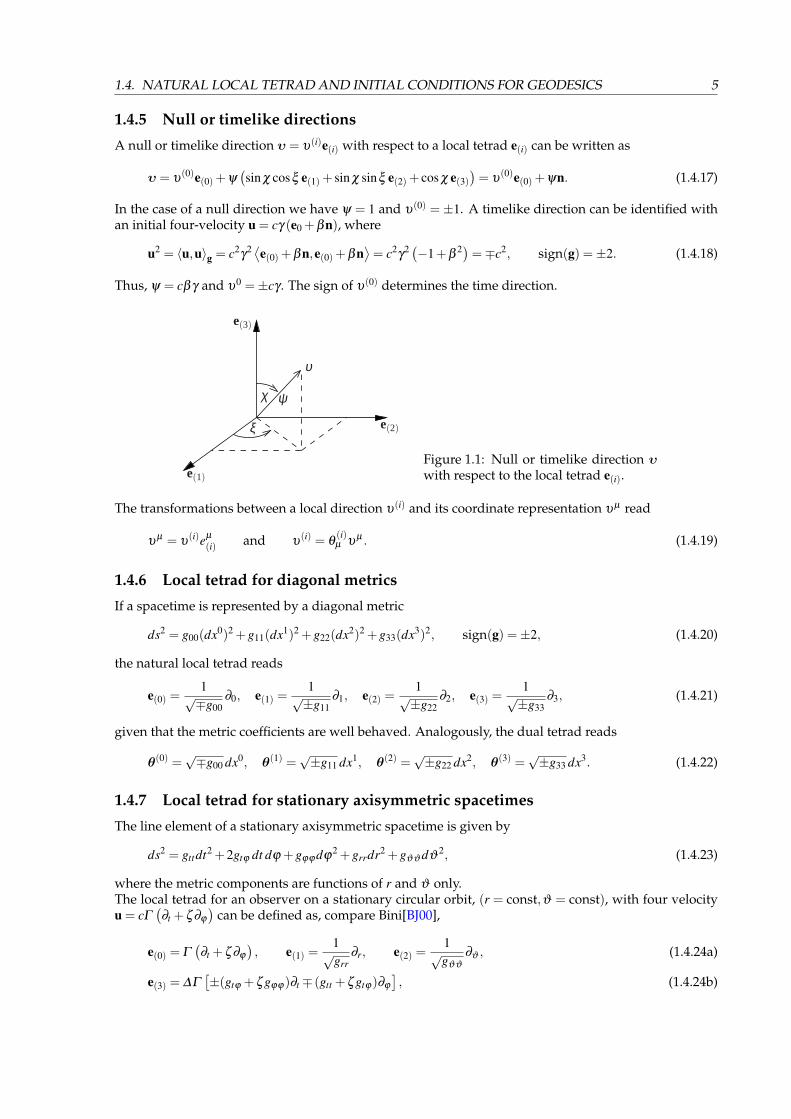
1.4.5 Null or timelike directions
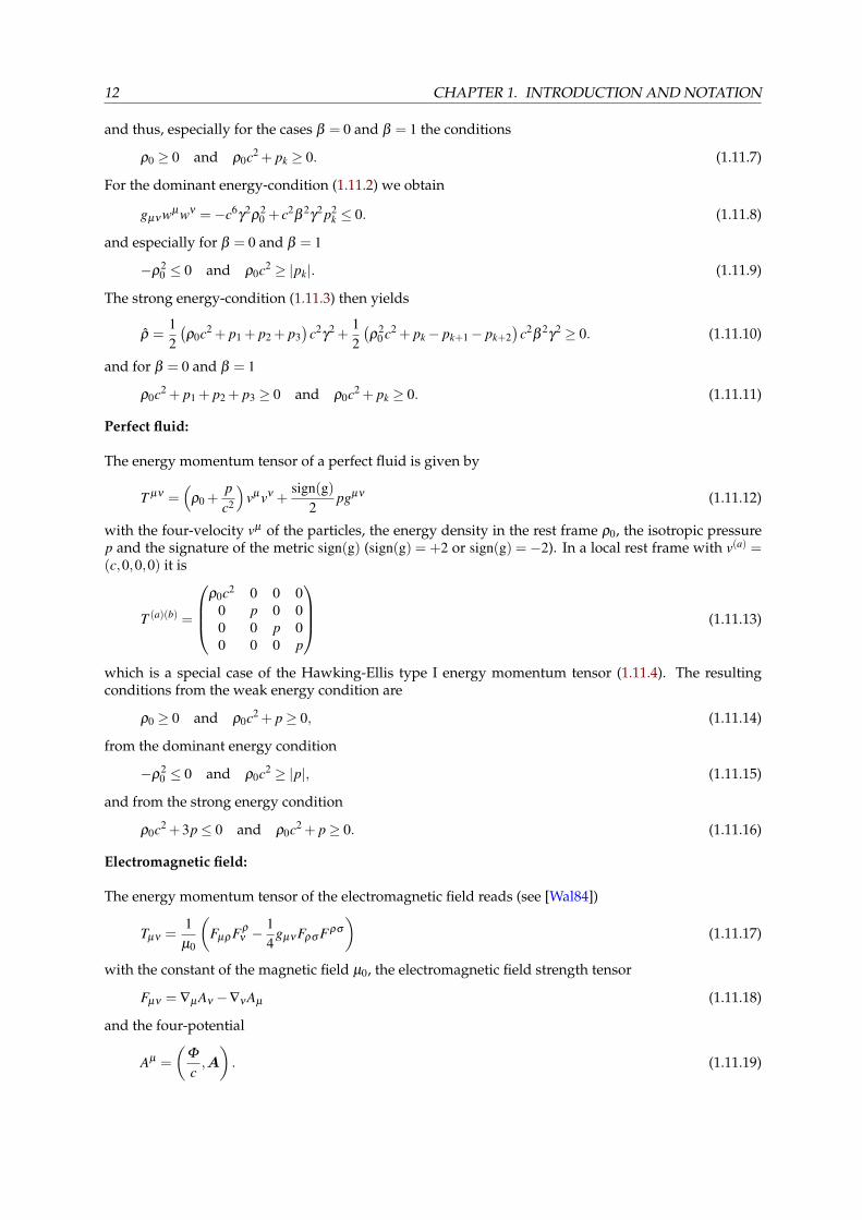
A null or timelike direction υ = υ(i)e(i) with respect to a local tetrad e(i) can be written as
υ = υ(0)e(0)+ψ
(sin χ cosξ e(1)+ sin χ sinξ e(2)+ cos χ e(3)
)= υ
(0)e(0)+ψn. (1.4.17)
In the case of a null direction we have ψ = 1 and υ(0) = ±1. A timelike direction can be identified withan initial four-velocity u = cγ (e0 +βn), where
u2 = 〈u,u〉g = c2γ
2 ⟨e(0)+βn,e(0)+βn⟩= c2
γ2 (−1+β
2)=∓c2, sign(g) =±2. (1.4.18)
Thus, ψ = cβγ and υ0 =±cγ . The sign of υ(0) determines the time direction.
e(1)
e(2)
e(3)
ξ
χ ψ
υ
Figure 1.1: Null or timelike direction υwith respect to the local tetrad e(i).
The transformations between a local direction υ(i) and its coordinate representation υµ read
υµ = υ
(i)eµ
(i) and υ(i) = θ
(i)µ υ
µ . (1.4.19)
1.4.6 Local tetrad for diagonal metrics
If a spacetime is represented by a diagonal metric
ds2 = g00(dx0)2 +g11(dx1)2 +g22(dx2)2 +g33(dx3)2, sign(g) =±2, (1.4.20)
the natural local tetrad reads
e(0) =1√∓g00
∂0, e(1) =1√±g11
∂1, e(2) =1√±g22
∂2, e(3) =1√±g33
∂3, (1.4.21)
given that the metric coefficients are well behaved. Analogously, the dual tetrad reads
θ(0) =√∓g00 dx0, θ(1) =
√±g11 dx1, θ(2) =√±g22 dx2, θ(3) =
ñg33 dx3. (1.4.22)
1.4.7 Local tetrad for stationary axisymmetric spacetimes
The line element of a stationary axisymmetric spacetime is given by
ds2 = gttdt2 +2gtϕ dt dϕ +gϕϕ dϕ2 +grrdr2 +gϑϑ dϑ
2, (1.4.23)
where the metric components are functions of r and ϑ only.The local tetrad for an observer on a stationary circular orbit, (r = const,ϑ = const), with four velocityu = cΓ
(∂t +ζ ∂ϕ
)can be defined as, compare Bini[BJ00],
e(0) = Γ(∂t +ζ ∂ϕ
), e(1) =
1√grr
∂r, e(2) =1√gϑϑ
∂ϑ , (1.4.24a)
e(3) = ∆Γ[±(gtϕ +ζ gϕϕ)∂t ∓ (gtt +ζ gtϕ)∂ϕ
], (1.4.24b)
6 CHAPTER 1. INTRODUCTION AND NOTATION
where
Γ =1√
−(gtt +2ζ gtϕ +ζ 2gϕϕ
) and ∆ =1√
g2tϕ −gttgϕϕ
. (1.4.25)
The angular velocity ζ is limited due to gtt +2ζ gtϕ +ζ 2gϕϕ < 0
ζmin = ω−√
ω2− gtt
gϕϕ
and ζmax = ω +
√ω2− gtt
gϕϕ
(1.4.26)
with ω =−gtϕ/gϕϕ .For ζ = 0, the observer is static with respect to spatial infinity. The locally non-rotating frame (LNRF)has angular velocity ζ = ω , see also MTW[MTW73], exercise 33.3.Static limit: ζmin = 0 ⇒ gtt = 0.The transformation between the local direction υ(i) and the coordinate direction υµ reads
υ0 = Γ
(υ(0)±υ
(3)∆w1
), υ
1 =υ(1)√
grr, υ
2 =υ(2)√
gϑϑ
, υ3 = Γ
(υ(0)
ζ ∓υ(3)
∆w2
), (1.4.27)
with
w1 = gtϕ +ζ gϕϕ and w2 = gtt +ζ gtϕ . (1.4.28)
The back transformation reads
υ(0) =
1Γ
υ0w2 +υ3w1
ζ w1 +w2, υ
(1) =√
grr υ1, υ
(2) =√
gϑϑ υ2, υ
(3) =± 1∆Γ
ζ υ0−υ3
ζ w1 +w2. (1.4.29)
Note, to obtain a right-handed local tetrad, det(
eµ
(i)
)> 0, the upper sign has to be used.
1.5 Newman-Penrose tetrad and spin-coefficients
The Newman-Penrose tetrad consists of four null vectors e?(i) = l,n,m,m, where l and n are real and mand m are complex conjugates; see Penrose and Rindler[PR84] or Chandrasekhar[Cha06] for a thoroughdiscussion. The Newman-Penrose (NP) tetrad has to fulfill the orthonormality relation
⟨e?(i),e
?( j)
⟩= η?(i)( j) with η?(i)( j) =
0 1 0 01 0 0 00 0 0 −10 0 −1 0
. (1.5.1)
A straightforward relation between the NP tetrad and the natural local tetrad, as discussed in Sec. 1.4,is given by
l =∓ 1√2
(e(0)+ e(1)
), n =∓ 1√
2
(e(0)− e(1)
), m =∓ 1√
2
(e(2)+ ie(3)
), (1.5.2)
where the upper/lower sign has to be used for metrics with positive/negative signature. The Riccirotation-coefficients of a NP tetrad are now called spin coefficients and are designated by specific symbols:
κ = γ(2)(1)(1), ρ = γ(2)(0)(3), ε =12(γ(1)(0)(0)+ γ(2)(3)(0)
), (1.5.3a)
σ = γ(2)(0)(2), µ = γ(1)(3)(2), γ =12(γ(1)(0)(1)+ γ(2)(3)(1)
), (1.5.3b)
λ = γ(1)(3)(3), τ = γ(2)(0)(1), α =12(γ(1)(0)(3)+ γ(2)(3)(3)
), (1.5.3c)
ν = γ(1)(3)(1), π = γ(1)(3)(0), β =12(γ(1)(0)(2)+ γ(2)(3)(2)
). (1.5.3d)
1.6. COORDINATE RELATIONS 7
1.6 Coordinate relations
1.6.1 Spherical and Cartesian coordinates
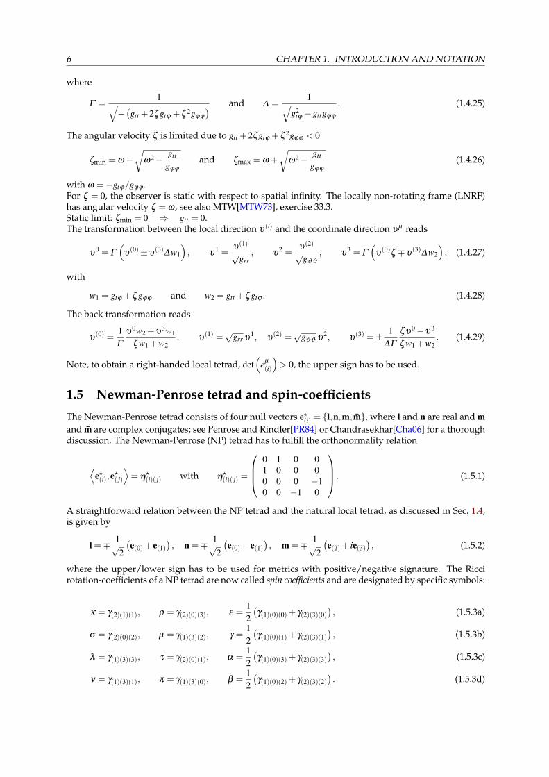
The well-known relation between the spherical coordinates (r,ϑ ,ϕ) and the Cartesian coordinates (x,y,z),compare Fig. 1.2, are
x = r sinϑ cosϕ, y = r sinϑ sinϕ, z = r cosϑ , (1.6.1)
and
r =√
x2 + y2 + z2, ϑ = arctan2(√
x2 + y2,z), ϕ = arctan2(y,x), (1.6.2)
where arctan2() ensures that ϕ ∈ [0,2π) and ϑ ∈ (0,π).
x
y
z
ϕ
ϑ r
Figure 1.2: Relation between sphericaland Cartesian coordinates.
The total differentials of the spherical coordinates read
dr =xdx+ ydy+ zdz
r, dϑ =
xzdx+ yzdy− (x2 + y2)dz
r2√
x2 + y2, dϕ =
−ydx+ xdyx2 + y2 , (1.6.3)
whereas the coordinate derivatives read
∂r =∂x∂ r
∂x +∂y∂ r
∂y +∂ z∂ r
∂z = sinϑ cosϕ ∂x + sinϑ sinϕ ∂y + cosϑ ∂z, (1.6.4a)
∂ϑ =∂x∂ϑ
∂x +∂y∂ϑ
∂y +∂ z∂ϑ
∂z = r cosϑ cosϕ ∂x + r cosϑ sinϕ ∂y− r sinϑ ∂z, (1.6.4b)
∂ϕ =∂x∂ϕ
∂x +∂y∂ϕ
∂y +∂ z∂ϕ
∂z =−r sinϑ sinϕ ∂x + r sinϑ cosϕ ∂y, (1.6.4c)
and
∂x =∂ r∂x
∂r +∂ϑ
∂x∂ϑ +
∂ϕ
∂x∂ϕ = sinϑ cosϕ ∂r +
cosϑ cosϕ
r∂ϑ −
sinϕ
r sinϑ∂ϕ , (1.6.5a)
∂y =∂ r∂y
∂r +∂ϑ
∂y∂ϑ +
∂ϕ
∂y∂ϕ = sinϑ sinϕ ∂r +
cosϑ sinϕ
r∂ϑ +
cosϕ
r sinϑ∂ϕ , (1.6.5b)
∂z =∂ r∂ z
∂r +∂ϑ
∂ z∂ϑ +
∂ϕ
∂ z∂ϕ = cosϑ ∂r−
sinϑ
r∂ϑ . (1.6.5c)
1.6.2 Cylindrical and Cartesian coordinates
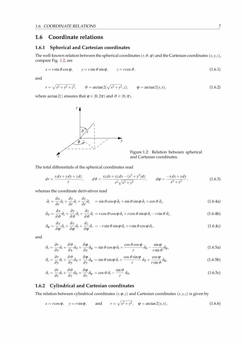
The relation between cylindrical coordinates (r,ϕ,z) and Cartesian coordinates (x,y,z) is given by
x = r cosϕ, y = r sinϕ, and r =√
x2 + y2, ϕ = arctan2(y,x), (1.6.6)
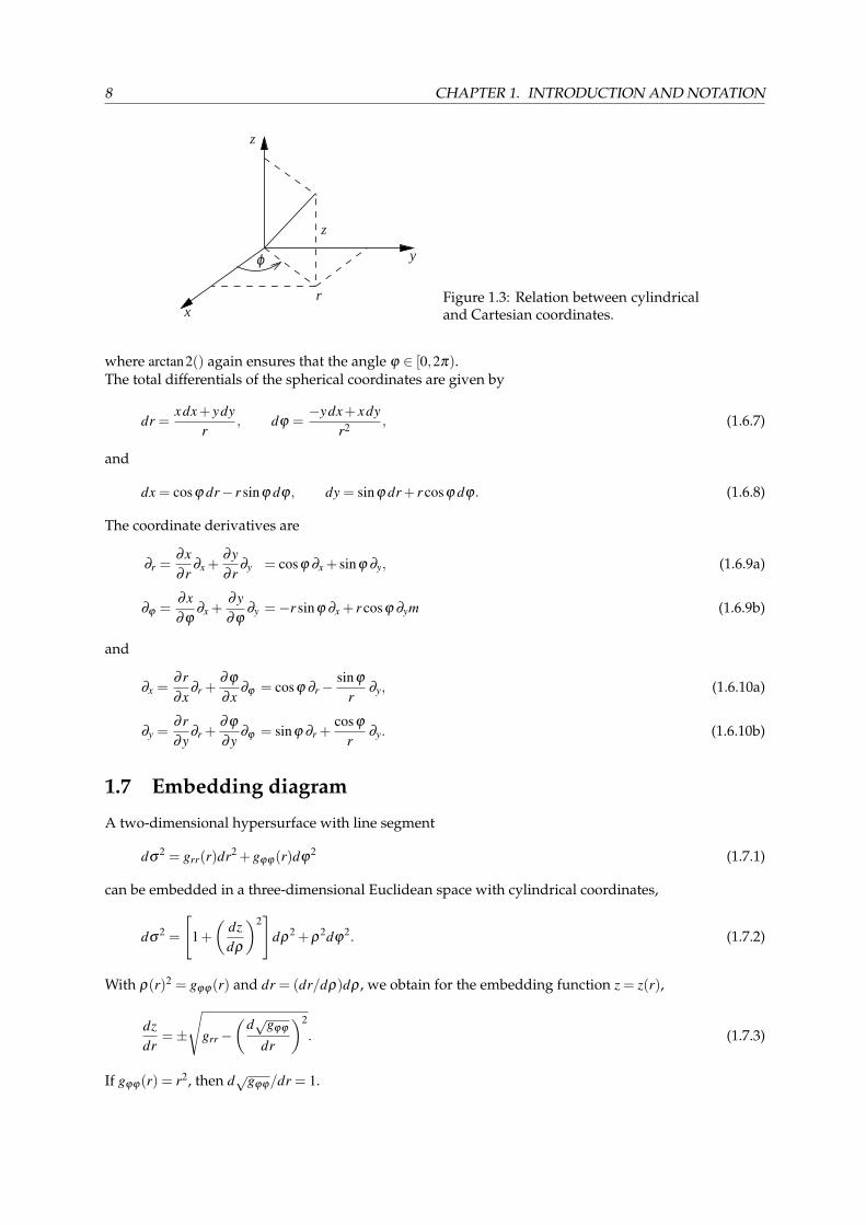
8 CHAPTER 1. INTRODUCTION AND NOTATION
x
y
z
ϕ
z
r Figure 1.3: Relation between cylindricaland Cartesian coordinates.
where arctan2() again ensures that the angle ϕ ∈ [0,2π).The total differentials of the spherical coordinates are given by
dr =xdx+ ydy
r, dϕ =
−ydx+ xdyr2 , (1.6.7)
and
dx = cosϕ dr− r sinϕ dϕ, dy = sinϕ dr+ r cosϕ dϕ. (1.6.8)
The coordinate derivatives are
∂r =∂x∂ r
∂x +∂y∂ r
∂y = cosϕ ∂x + sinϕ ∂y, (1.6.9a)
∂ϕ =∂x∂ϕ
∂x +∂y∂ϕ
∂y =−r sinϕ ∂x + r cosϕ ∂ym (1.6.9b)
and
∂x =∂ r∂x
∂r +∂ϕ
∂x∂ϕ = cosϕ ∂r−
sinϕ
r∂y, (1.6.10a)
∂y =∂ r∂y
∂r +∂ϕ
∂y∂ϕ = sinϕ ∂r +
cosϕ
r∂y. (1.6.10b)
1.7 Embedding diagram
A two-dimensional hypersurface with line segment
dσ2 = grr(r)dr2 +gϕϕ(r)dϕ
2 (1.7.1)
can be embedded in a three-dimensional Euclidean space with cylindrical coordinates,
dσ2 =
[1+(
dzdρ
)2]
dρ2 +ρ
2dϕ2. (1.7.2)
With ρ(r)2 = gϕϕ(r) and dr = (dr/dρ)dρ , we obtain for the embedding function z = z(r),
dzdr
=±√
grr−(
d√gϕϕ
dr
)2
. (1.7.3)
If gϕϕ(r) = r2, then d√gϕϕ/dr = 1.
1.8. EQUATIONS OF MOTION AND TRANSPORT EQUATIONS 9
1.8 Equations of motion and transport equations
1.8.1 Geodesic equation
The geodesic equation reads
D2xµ
dλ 2 =d2xµ
dλ 2 +Γµ
ρσ
dxρ
dλ
dxσ
dλ= 0 (1.8.1)
with the affine parameter λ . For timelike geodesics, however, we replace the affine parameter by theproper time τ .The geodesic equation (1.8.1) is a system of ordinary differential equations of second order. Hence, tosolve these differential equations, we need an initial position xµ(λ = 0) as well as an initial direction(dxµ/dλ )(λ = 0). This initial direction has to fulfill the constraint equation
gµν
dxµ
dλ
dxν
dλ= κc2, (1.8.2)
where κ = 0 for lightlike and κ =∓1, (sign(g) =±2), for timelike geodesics.The initial direction can also be determined by means of a local reference frame, compare sec. 1.4.5, thatautomatically fulfills the constraint equation (1.8.2). If we use the natural local tetrad as local referenceframe, we have
dxµ
dλ
∣∣∣∣λ=0
= υµ = υ
(i)eµ
(i). (1.8.3)
1.8.2 Fermi-Walker transport
The Fermi-Walker transport, see e.g. Stephani[SS90], of a vector X = X µ ∂µ along the worldline xµ(τ)with four-velocity u = uµ(τ)∂µ is given by FuX µ = 0 with
FuX µ :=dX µ
dτ+Γ
µ
ρσ uρ Xσ +1c2 (u
σ aµ −aσ uµ)gρσ Xρ . (1.8.4)
The four-acceleration follows from the four-velocity via
aµ =D2xµ
dτ2 =Duµ
dτ=
duµ
dτ+Γ
µ
ρσ uρ uσ . (1.8.5)
1.8.3 Parallel transport
If the four-acceleration vanishes, the Fermi-Walker transport simplifies to the parallel transport PuX µ = 0with
PuX µ :=DX µ
dτ=
dX µ
dτ+Γ
µ
ρσ uρ Xσ . (1.8.6)
1.8.4 Euler-Lagrange formalism
A detailed discussion of the Euler-Lagrange formalism can be found, e.g., in Rindler[Rin01]. The La-grangian L is defined as
L := gµν xµ xν , L!= κc2, (1.8.7)
where xµ are the coordinates of the metric, and the dot means differentiation with respect to the affineparameter λ . For timelike geodesics, κ =∓1 depending on the signature of the metric, sign(g) =±2. Forlightlike geodesics, κ = 0.
10 CHAPTER 1. INTRODUCTION AND NOTATION
The Euler-Lagrange equations read
ddλ
∂L
∂ xµ− ∂L
∂xµ= 0. (1.8.8)
If L is independent of xρ , then xρ is a cyclic variable and
pρ = gρν xν = const. (1.8.9)
Note that [L ]U =length2
time2 for timelike and [L ]U = 1 for lightlike geodesics, see Sec. 1.10.
1.8.5 Hamilton formalism
The super-Hamiltonian H is defined as
H :=12
gµν pµ pν , H!=
12
κc2, (1.8.10)
where pµ = gµν xν are the canonical momenta, see e.g. MTW[MTW73], para. 21.1. As in classical me-chanics, we have
dxµ
dλ=
∂H
∂ pµ
anddpµ
dλ=−∂H
∂xµ. (1.8.11)
1.9 Special topics
1.9.1 Timelike circular geodesics
Given a spacetime in spherical or polar coordinates, timelike circular geodesics with respect to the radialcoordinate can be found by means of the equation for acceleration
aµ =duµ
dτ+Γ
µ
νλuν uλ (1.9.12)
and the ansatz for the four-velocity u = cγ(e(t)+βe(ϕ)
)= ut∂t +uϕ ∂ϕ with γ = 1/
√1−β 2. To be geodetic,
all components of the four-acceleration (1.9.12) must vanish. Because u = const, duµ/dτ = 0. In sphericalcoordinates, the remaining equations read
at = Γt
tt utut +2Γ
ttϕ utuϕ +Γ
tϕϕ uϕ uϕ = c2
γ2[Γ
ttt e
t(t)e
t(t)+2βΓ
ttϕ et
(t)et(ϕ)+β
2Γ
tϕϕ et
(ϕ)et(ϕ)
]!= 0, (1.9.13a)
ar = Γr
tt utut +2Γr
tϕ utuϕ +Γr
ϕϕ uϕ uϕ = c2γ
2[Γ
rtt et
(t)et(t)+2βΓ
rtϕ et
(t)et(ϕ)+β
2Γ
rϕϕ et
(ϕ)et(ϕ)
]!= 0, (1.9.13b)
aϑ = Γϑ
tt utut +2Γϑ
tϕ utuϕ +Γϑ
ϕϕ uϕ uϕ = c2γ
2[Γ
ϑtt et
(t)et(t)+2βΓ
ϑtϕ et
(t)et(ϕ)+β
2Γ
ϑϕϕ et
(ϕ)et(ϕ)
]!= 0, (1.9.13c)
aϕ = Γϕ
tt utut +2Γϕ
tϕ utuϕ +Γϕ
ϕϕ uϕ uϕ = c2γ
2[Γ
ϕ
tt et(t)e
t(t)+2βΓ
ϕ
tϕ et(t)e
t(ϕ)+β
2Γ
ϕ
ϕϕ et(ϕ)e
t(ϕ)
]!= 0. (1.9.13d)
1.10 Units
A first test in analyzing whether an equation is correct is to check the units. Newton’s gravitationalconstant G, for example, has the following units
[G]U =length3
mass · time2 , (1.10.1)
where [·]U indicates that we evaluate the units of the enclosed expression. Further examples are
[ds]U = length, [u]U =lengthtime
, [RSchwarzschildtrtr ]U =
1time2 ,
[RSchwarzschild
ϑϕϑϕ
]U= length2. (1.10.2)
1.11. ENERGY MOMENTUM TENSOR 11
1.11 Energy momentum tensor
The Einstein field equations (1.2.1) connect the geometry of the spacetime with the density of the energyand the momenta. For a given energy momentum tensor Tµν , they are a differential system for thespacetime components gµν . On the other hand, they give us the energy momentum tensor for a givenspacetime geometry. In this case, Tµν has to satisfy the so called energy conditions to guarantee that themetric is physically reasonable. These conditions go back to Hawking and Ellis [HE99].
1.11.1 Energy conditions
Weak energy condition:
An observer moving with the four-velocity uµ measures the local energy density ρ := Tµν uµ uν . It has tobe non-negative for all causal uµ , that means for all timelike and lightlike uµ :
ρ = Tµν uµ uν ≥ 0. (1.11.1)
For lightlike uµ this is also called null energy condition.
Dominant energy condition:
An observer moving with the four-velocity uµ with Tµν uµ uν ≥ 0 measures the local energy flux wµ :=T µν uν which has to be also a causal four-vector for all uµ . For the metric signature +2, this conditionreads
gµν wµ wν ≤ 0. (1.11.2)
Strong energy condition:
The tidal energy momentum tensor is defined by Tµν := Tµν− 12 T gµν . The corresponding energy density
ρ := Tµν uµ uν has to be non-negative for all causal four-velocities uµ :
ρ =
(Tµν −
12
T gµν
)uµ uν ≥ 0. (1.11.3)
1.11.2 Examples for energy momentum tensors
Hawking-Ellis type I:
The energy momentum tensor for an observer whose world-line has the unit tangent vector e0 is
T (a)(b) =
ρ0c2 0 0 0
0 p1 0 00 0 p2 00 0 0 p3
(1.11.4)
with the local energy density ρ0 and the pressures pi in the three spacelike directions (see [HE99]). Wewill consider a four-velocity with respect to the same local tetrad as T (a)(b). The observer moves withoutloss of generality in e(k)-direction (k ∈ 1,2,3). Thus, it is
uµ = (u(0),u(k)e(k)) (1.11.5)
with u(0) = cγ and u(k) = cβγ in the timelike and u(0) = u(k) = 1 in the lightlike case. The weak energycondition (1.11.1) yields
ρ = Tµν uµ uν = ρ0c4γ
2 + pkc2β
2γ
2 ≥ 0 (1.11.6)
12 CHAPTER 1. INTRODUCTION AND NOTATION
and thus, especially for the cases β = 0 and β = 1 the conditions
ρ0 ≥ 0 and ρ0c2 + pk ≥ 0. (1.11.7)
For the dominant energy-condition (1.11.2) we obtain
gµν wµ wν =−c6γ
2ρ
20 + c2
β2γ
2 p2k ≤ 0. (1.11.8)
and especially for β = 0 and β = 1
−ρ20 ≤ 0 and ρ0c2 ≥ |pk|. (1.11.9)
The strong energy-condition (1.11.3) then yields
ρ =12(ρ0c2 + p1 + p2 + p3
)c2
γ2 +
12(ρ
20 c2 + pk− pk+1− pk+2
)c2
β2γ
2 ≥ 0. (1.11.10)
and for β = 0 and β = 1
ρ0c2 + p1 + p2 + p3 ≥ 0 and ρ0c2 + pk ≥ 0. (1.11.11)
Perfect fluid:
The energy momentum tensor of a perfect fluid is given by
T µν =(
ρ0 +pc2
)vµ vν +
sign(g)2
pgµν (1.11.12)
with the four-velocity vµ of the particles, the energy density in the rest frame ρ0, the isotropic pressurep and the signature of the metric sign(g) (sign(g) = +2 or sign(g) = −2). In a local rest frame with v(a) =(c,0,0,0) it is
T (a)(b) =
ρ0c2 0 0 0
0 p 0 00 0 p 00 0 0 p
(1.11.13)
which is a special case of the Hawking-Ellis type I energy momentum tensor (1.11.4). The resultingconditions from the weak energy condition are
ρ0 ≥ 0 and ρ0c2 + p≥ 0, (1.11.14)
from the dominant energy condition
−ρ20 ≤ 0 and ρ0c2 ≥ |p|, (1.11.15)
and from the strong energy condition
ρ0c2 +3p≤ 0 and ρ0c2 + p≥ 0. (1.11.16)
Electromagnetic field:
The energy momentum tensor of the electromagnetic field reads (see [Wal84])
Tµν =1µ0
(Fµρ Fρ
ν −14
gµν Fρσ Fρσ
)(1.11.17)
with the constant of the magnetic field µ0, the electromagnetic field strength tensor
Fµν = ∇µ Aν −∇ν Aµ (1.11.18)
and the four-potential
Aµ =
(Φ
c,A
). (1.11.19)
1.12. TOOLS 13
1.12 Tools
1.12.1 Maple/GRTensorIIThe Christoffel symbols, the Riemann- and Ricci-tensors as well as the Ricci and Kretschmann scalars inthis catalogue were determined by means of the software Maple together with the GRTensorII packageby Musgrave, Pollney, and Lake.2
A typical worksheet to enter a new metric may look like this:
> grtw();> makeg(Schwarzschild);
Makeg 2.0: GRTensor metric/basis entry utilityTo quit makeg, type ’exit’ at any prompt.Do you wish to enter a 1) metric [g(dn,dn)],
2) line element [ds],3) non-holonomic basis [e(1)...e(n)], or4) NP tetrad [l,n,m,mbar]?
> 2:
Enter coordinates as a LIST (eg. [t,r,theta,phi]):> [t,r,theta,phi]:
Enter the line element using d[coord] to indicate differentials.(for example, r^2*(d[theta]^2 + sin(theta)^2*d[phi]^2)[Type ’exit’ to quit makeg]ds^2 =
If there are any complex valued coordinates, constants or functionsfor this spacetime, please enter them as a SET ( eg. z, psi ).
Complex quantities [default=]:> :
You may choose to 0) Use the metric WITHOUT saving it,1) Save the metric as it is,2) Correct an element of the metric,3) Re-enter the metric,4) Add/change constraint equations,5) Add a text description, or6) Abandon this metric and return to Maple.
> 0:
The worksheets for some of the metrics in this catalogue can be found on the authors homepage. Todetermine the objects that are defined with respect to a local tetrad, the metric must be given as non-holonomic basis.The various basic objects can be determined via
Christoffel symbols Γµ
νρ grcalc(Chr2); grcalc(Chr(dn,dn,up));partial derivatives Γ
µ
νρ,σ grcalc(Chr(dn,dn,up,pdn));Riemann tensor Rµνρσ grcalc(Riemman); grcalc(R(dn,dn,dn,dn));Ricci tensor Rµν grcalc(Ricci); grcalc(R(dn,dn));Ricci scalar R grcalc(Ricciscalar);Kretschmann scalar K grcalc(RiemSq);
1.12.2 MathematicaThe calculation of the Christoffel symbols, the Riemann- or Ricci-tensor within Mathematica could readlike this:
Clearing the values of symbols:In[1]:= Clear[coord, metric, inversemetric, affine,
2The commercial software Maple can be found here: http://www.maplesoft.com. The GRTensorII-package is free:http://grtensor.phy.queensu.ca.
14 CHAPTER 1. INTRODUCTION AND NOTATION
t, r, Theta, Phi]
Setting the dimension:In[2]:= n := 4
Defining a list of coordinates:In[3]:= coord := t, r, Theta, Phi
Defining the metric:In[4]:= metric := -(1 - rs/r) c^2, 0, 0, 0,
0, 1/(1 - rs/r), 0, 0,0, 0, r^2, 0,0, 0, 0, r ^2 Sin[Theta]^2
In[5]:= metric // MatrixForm
Calculating the inverse metric:In[6]:= inversemetric := Simplify[Inverse[metric]]
In[7]:= inversemetric // MatrixForm
Calculating the Christoffel symbols of the second kind:In[8]:= affine := affine = Simplify[
Table[(1/2) Sum[inversemetric[[Mu, Rho]] (D[metric[[Rho, Nu]], coord[[Lambda]]] +D[metric[[Rho, Lambda]], coord[[Nu]]] -D[metric[[Nu, Lambda]], coord[[Rho]]]),
Rho, 1, n], Nu, 1, n, Lambda, 1, n, Mu, 1, n]]
Displaying the Christoffel symbols of the second kind:In[9]:= listaffine :=
Table[If[UnsameQ[affine[[Nu, Lambda, Mu]], 0],Style[ Subsuperscript[\[CapitalGamma],
Row[coord[[Nu]], coord[[Lambda]]], coord[[Mu]]], 18],"=",Style[affine[[Nu, Lambda, Mu]], 14]],
Lambda, 1, n, Nu, 1, Lambda, Mu, 1, n]
In[10]:= TableForm[Partition[DeleteCases[Flatten[listaffine],Null], 3],
TableSpacing -> 1, 2]
Defining the Riemann tensor:In[11]:= riemann := riemann =Table[D[affine[[Nu, Sigma, Mu]], coord[[Rho]]] -
D[affine[[Nu, Rho, Mu]], coord[[Sigma]]] +Sum[affine[[Rho, Lambda, Mu]]
affine[[Nu, Sigma, Lambda]] -affine[[Sigma, Lambda, Mu]]affine[[Nu, Rho, Lambda]],
Lambda, 1, n],Mu, 1, n, Nu, 1, n, Rho, 1, n, Sigma, 1, n]
Defining the Riemann tensor with lower indices:In[12]:= riemannDn := riemannDn =Table[Simplify[
Sum[metric[[Mu, Kappa]] riemann[[Kappa, Nu, Rho, Sigma]],Kappa, 1, n]],
Mu, 1, n, Nu, 1, n, Rho, 1, n, Sigma, 1, n]
In[13]:= listRiemann :=Table[If[UnsameQ[riemannDn[[Mu, Nu, Rho, Sigma]], 0],Style[Subscript[R, Row[coord[[Mu]], coord[[Nu]], coord[[Rho]],
coord[[Sigma]]]], 16], "=",riemannDn[[Mu, Nu, Rho, Sigma]]],
Nu, 1, n, Mu, 1, Nu, Sigma, 1, n, Rho, 1, Sigma]
In[14]:= TableForm[Partition[DeleteCases[Flatten[listRiemann],Null], 3],
TableSpacing -> 2, 2]
Defining the Ricci tensor:In[15]:= ricci := ricci =
Table[Simplify[Sum[riemann[[Rho, Mu, Rho, Nu]], Rho, 1, n]],
1.12. TOOLS 15
Mu, 1, n, Nu, 1, n]
In[16]:= listRicci :=Table[If[UnsameQ[ricci[[Mu, Nu]], 0],
Style[Subscript[R, Row[coord[[Mu]], coord[[Nu]]]], 16],"=",
Style[ricci[[Mu, Nu]], 16]], Nu, 1, 4, Mu, 1, Nu]
In[17]:= TableForm[Partition[DeleteCases[Flatten[listRicci],Null], 3],
TableSpacing -> 1, 2]
Defining the Ricci scalar:In[18]:= ricciscalar := ricciscalar =
Simplify[Sum[Sum[inversemetric[[Mu, Nu]] ricci[[Nu, Mu]],Mu, 1, n], Nu, 1, n]]
Defining the Kretschmann scalar:In[19]:= riemannUp := riemannUp =
Table[Simplify[Sum[inversemetric[[Nu, Kappa]]
riemann[[Mu, Kappa, Rho, Sigma]], Kappa, 1, n]],Mu, 1, n, Nu, 1, n, Rho, 1, n, Sigma, 1, n]
In[20]:= kretschmann := kretschmann =Simplify[Sum[ Sum[Sum[Sum[
riemannUp[[Mu, Nu, Rho, Sigma]]riemannUp[[Rho, Sigma, Mu, Nu]],Mu, 1, n], Nu, 1, n], Rho, 1, n], Sigma, 1, n]]
Some example notebooks can be found on the authors homepage.
1.12.3 MaximaInstead of using commercial software like Maple or Mathematica, Maxima also offers a tensor packagethat helps to calculate the Christoffel symbols etc. The above example for the Schwarzschild metric canbe written as a maxima worksheet as follows:
/* load ctensor package */load(ctensor);
/* define coordinates to use */ct_coords:[t,r,theta,phi];
/* start with the identity metric */lg:ident(4);lg[1,1]:-c^2*(1-rs/r);lg[2,2]:1/(1-rs/r);lg[3,3]:r^2;lg[4,4]:r^2*sin(theta)^2;
/* computes the metric inverse and sets up the package for further calculations. */cmetric();
/* calculate the christoffel symbols of the second kind */christof(mcs);
/* calculate the riemann tensorNote the different ordering of the indices:R[mu,nu,rho,sigma]=lriem[nu,sigma,rho,mu]
*/lriemann(true);RM(mu,nu,rho,sigma):=lriem[nu,sigma,rho,mu];
/* calculate the ricci tensor */ricci(true);
/* simplify the ricci tensor */ratsimp(ric[1,1]);ratsimp(ric[2,2]);
16 CHAPTER 1. INTRODUCTION AND NOTATION
/* calculate the ricci scalar */scurvature();
/* calculate the Kretschmann scalar */uriemann(false);rinvariant();ratsimp(%);
Here, we have used maxima version 5.20.1.
1.12.4 Sympy
Another alternative to commercial software is the SymPy package for python. The m4d module is par-tially based on...
import sysfrom sympy import *
class Metric(object):"""
Turn matrix into upper and lower metric"""def __init__(self,m):
self.gdd = mself.guu = m.inv()
def __str__(self):return "g_dd = \n" + str(self.gdd)
def dd(self,i,j):return self.gdd[i,j]
def uu(self,i,j):return self.guu[i,j]
class Gamma(object):"""
Calculate Christoffel Gamma_ij^k symbols of metric g"""def __init__(self,g,x):
self.g = gself.x = x
def ddu(self,i,j,k):g = self.gx = self.xchr = 0for m in [0,1,2,3]:
chr += g.uu(k,m)/2 * (g.dd(m,i).diff(x[j]) \+ g.dd(m,j).diff(x[i]) - g.dd(i,j).diff(x[m]))
#return chr.simplify()return chr
class Riemann(object):"""
Calculate Riemann tensor R^mu_nu,rho,sigma"""def __init__(self,g,G,x):
self.g = gself.G = Gself.x = x
def uddd(self,mu,nu,rho,sigma):G = self.Gx = self.xR = G.ddu(nu,sigma,mu).diff(x[rho]) - G.ddu(nu,rho,mu).diff(x[sigma])for lam in [0,1,2,3]:
R += G.ddu(rho,lam,mu)*G.ddu(nu,sigma,lam) - \G.ddu(sigma,lam,mu)*G.ddu(nu,rho,lam)
return R.simplify()
def dddd(self,mu,nu,rho,sigma):
1.12. TOOLS 17
g = self.gR = 0for lam in [0,1,2,3]:
R += g.dd(mu,lam)*self.uddd(lam,nu,rho,sigma)return R.simplify()
class Ricci(object):"""
Calculate Ricci tensor from Riemann tensor"""def __init__(self,R):
self.R = R
def dd(self,mu,nu):R = self.RRic = 0for rho in [0,1,2,3]:
Ric += R.uddd(rho,mu,rho,nu)return Ric.simplify()
class RicciScalar(object):"""
Calculate Ricci scalar from Ricci tensor"""def __init__(self,Ric,g):
self.Ric = Ricself.g = g
def value(self):Ric = self.Ricg = self.gRS = 0for mu in [0,1,2,3]:
for nu in [0,1,2,3]:RS += g.uu(mu,nu)*Ric.dd(mu,nu)
return RS.simplify()
def pprint_christoffel_ddu(Gamma,i,j,k):pprint(Eq(Symbol(’Chr_%i%i^%i’ % (i,j,k)), Gamma.ddu(i,j,k)))
def pprint_christoffels(Gamma):for i in [0,1,2,3]:
for j in [0,1,2,3]:for k in [0,1,2,3]:
if (Gamma.ddu(i,j,k)!=0):pprint_christoffel_ddu(Gamma,i,j,k)
def pprint_riemann(Riemann):for i in [0,1,2,3]:
for j in [0,1,2,3]:for k in [0,1,2,3]:
for m in [0,1,2,3]:if (Riemann.uddd(i,j,k,m)!=0):
pprint(Eq(Symbol(’R^%i_%i%i%i’ % (i,j,k,m)), Riemann.uddd(i,j,k,m)))
def pprint_riemann_down(Riemann):for i in [0,1,2,3]:
for j in [0,1,2,3]:for k in [0,1,2,3]:
for m in [0,1,2,3]:if (Riemann.uddd(i,j,k,m)!=0):
pprint(Eq(Symbol(’R_%i%i%i%i’ % (i,j,k,m)), Riemann.dddd(i,j,k,m)))
def codeprint_metric(g,f=sys.stdout):for i in [0,1,2,3]:
for j in [0,1,2,3]:print >>f, "g_compts[0][1] = 2;".format(i,j,ccode(g.dd(i,j)))
def codeprint_christoffels(Gamma,f=sys.stdout):for i in [0,1,2,3]:
for j in [0,1,2,3]:for k in [0,1,2,3]:
print >>f, "christoffel[0][1][2] = 3;".format(i,j,k,ccode(Gamma.ddu(i,j,k)))
18 CHAPTER 1. INTRODUCTION AND NOTATION
def codeprint_chrisD(Gamma,X,f=sys.stdout):for i in [0,1,2,3]:
for j in [0,1,2,3]:for k in [0,1,2,3]:
for m in [0,1,2,3]:print >>f, "chrisD[0][1][2][3] = 4;"
.format(i,j,k,m,ccode(Gamma.ddu(i,j,k).diff(X[m]).simplify()))
def codeprint_riem(Riemann,f=sys.stdout):for i in [0,1,2,3]:
for j in [0,1,2,3]:for k in [0,1,2,3]:
for m in [0,1,2,3]:print >>f, "riem[0][1][2][3] = 4;".format(i,j,k,m,ccode(Riemann.uddd(i,j,k,m)))
def codeprint_ricci(Ricci,f=sys.stdout):for i in [0,1,2,3]:
for j in [0,1,2,3]:print >>f, "ricci[0][1] = 2".format(i,j,ccode(Ricci.dd(i,j)))
Chapter 2
Spacetimes
2.1 Minkowski
2.1.1 Cartesian coordinates
The Minkowski metric in Cartesian coordinates t,x,y,z ∈R reads
ds2 =−c2dt2 +dx2 +dy2 +dz2. (2.1.1)
All Christoffel symbols as well as the Riemann- and Ricci-tensor vanish identically. The natural localtetrad is trivial,
e(t) =1c
∂t , e(x) = ∂x, e(y) = ∂y, e(z) = ∂z, (2.1.2)
with dual
θ(t) = cdt, θ(x) = dx, θ(y) = dy, θ(z) = dz. (2.1.3)
2.1.2 Cylindrical coordinates
The Minkowski metric in cylindrical coordinates t ∈R,r ∈R+,ϕ ∈ [0,2π),z ∈R,
ds2 =−c2dt2 +dr2 + r2dϕ2 +dz2, (2.1.4)
has the natural local tetrad
e(t) =1c
∂t , e(r) = ∂r, e(ϕ) =1r
∂ϕ , e(z) = ∂z. (2.1.5)
Christoffel symbols:
Γr
ϕϕ =−r, Γϕ
rϕ =1r. (2.1.6)
Partial derivatives
Γϕ
rϕ,r =−1r2 , Γ
rϕϕ,r =−1. (2.1.7)
Ricci rotation coefficients:
γ(ϕ)(r)(ϕ) =1r
and γ(r) =1r. (2.1.8)
19
20 CHAPTER 2. SPACETIMES
2.1.3 Spherical coordinates
In spherical coordinates t ∈R,r ∈R+,ϑ ∈ (0,π),ϕ ∈ [0,2π), the Minkowski metric reads
ds2 =−c2dt2 +dr2 + r2 (dϑ2 + sin2
ϑdϕ2) . (2.1.9)
Christoffel symbols:
Γr
ϑϑ =−r, Γr
ϕϕ =−r sin2ϑ , Γ
ϑrϑ =
1r, (2.1.10a)
Γϑ
ϕϕ =−sinϑ cosϑ , Γϕ
rϕ =1r, Γ
ϕ
ϑϕ= cotϑ . (2.1.10b)
Partial derivatives
Γϑ
rϑ ,r =−1r2 , Γ
ϕ
rϕ,r =−1r2 , Γ
rϑϑ ,r =−1, (2.1.11a)
Γϕ
ϑϕ,ϑ =− 1sin2
ϑ, Γ
rϕϕ,r =−sin2
ϑ , Γϑ
ϕϕ,ϑ =−cos(2ϑ), (2.1.11b)
Γr
ϕϕ,ϑ =−sin(2ϑ). (2.1.11c)
Local tetrad:
e(t) =1c
∂t , e(r) = ∂r, e(ϑ) =1r
∂ϑ , e(ϕ) =1
r sinϑ∂ϕ . (2.1.12)
Ricci rotation coefficients:
γ(ϑ)(r)(ϑ) = γ(ϕ)(r)(ϕ) =1r, γ(ϕ)(ϑ)(ϕ) =
cotϑ
r. (2.1.13)
The contractions of the Ricci rotation coefficients read
γ(r) =2r, γ(ϑ) =
cotϑ
r. (2.1.14)
2.1.4 Conform-compactified coordinates
The Minkowski metric in conform-compactified coordinates ψ ∈ [−π,π],ξ ∈ (0,π),ϑ ∈ (0,π),ϕ ∈ [0,2π)reads[HE99]
ds2 =−dψ2 +dξ
2 + sin2ξ(dϑ
2 + sin2ϑdϕ
2) . (2.1.15)
This form follows from the spherical Minkowski metric (2.1.9) by means of the coordinate transforma-tion
ct + r = tanψ +ξ
2, ct− r = tan
ψ−ξ
2, (2.1.16)
resulting in the metric
ds2 =−dψ2 +dξ 2
4cos2 ψ+ξ
2 cos2 ψ−ξ
2
+sin2
ξ
4cos2 ψ+ξ
2 cos2 ψ−ξ
2
(dϑ
2 + sin2ϑdϕ
2) , (2.1.17)
and by the conformal transformation ds2 = Ω 2ds2 with Ω 2 = 4cos2 ψ+ξ
2 cos2 ψ−ξ
2 .Christoffel symbols:
Γϑ
ξ ϑ= cotξ , Γ
ϕ
ξ ϕ= cotξ , Γ
ξ
ϑϑ=−sinξ cosξ , (2.1.18a)
Γϕ
ϑϕ= cotϑ , Γ
ξ
ϕϕ =−sinξ cosξ sin2ϑ , Γ
ϑϕϕ =−sinϑ cosϑ . (2.1.18b)
2.1. MINKOWSKI 21
Partial derivatives
Γϑ
ξ ϑ ,ξ =− 1sin2
ξ, Γ
ϕ
ξ ϕ,ξ=− 1
sin2ξ, Γ
ξ
ϑϑ ,ξ=−cos(2ξ ), (2.1.19a)
Γϕ
ϑϕ,ϑ =− 1sin2
ϑ, Γ
ξ
ϕϕ,ξ=−cos(2ξ )sin2
ϑ , Γϑ
ϕϕ,ϑ =−cos(2ϑ), (2.1.19b)
Γξ
ϕϕ,ϑ =−12
sin(2ξ )sin(2ϑ). (2.1.19c)
Riemann-Tensor:
Rξ ϑξ ϑ = sin2ξ , Rξ ϕξ ϕ = sin2
ξ sin2ϑ , Rϑϕϑϕ = sin4
ξ sin2ϑ . (2.1.20)
Ricci-Tensor:
Rξ ξ = 2, Rϑϑ = 2sin2ξ , Rϕϕ = 2sin2
ξ sin2ϑ . (2.1.21)
Ricci and Kretschmann scalars:
R = 6, K = 12. (2.1.22)
The Weyl tensor vanishs identically.Local tetrad:
e(ψ) = ∂ψ , e(ξ ) = ∂ξ , e(ϑ) =1
sinξ∂ϑ , e(ϕ) =
1sinξ sinϑ
∂ϕ . (2.1.23)
Ricci rotation coefficients:
γ(ϑ)(ξ )(ϑ) = γ(ϕ)(ξ )(ϕ) = cotξ , γ(ϕ)(ϑ)(ϕ) =cotϑ
sinξ. (2.1.24)
The contractions of the Ricci rotation coefficients read
γ(ξ ) = 2cotξ , γ(ϑ) =cotϑ
sinξ. (2.1.25)
Riemann-Tensor with respect to local tetrad:
R(ξ )(ϑ)(ξ )(ϑ) = R(ξ )(ϕ)(ξ )(ϕ) = R(ϑ)(ϕ)(ϑ)(ϕ) = 1. (2.1.26)
Ricci-Tensor with respect to local tetrad:
R(ξ )(ξ ) = R(ϑ)(ϑ) = R(ϕ)(ϕ) = 2. (2.1.27)
2.1.5 Rotating coordinates
The transformation dϕ 7→ dϕ +ω dt brings the Minkowski metric (2.1.4) into the rotating form[Rin01]with coordinates t ∈R,r ∈R+,ϕ ∈ [0,2π),z ∈R,
ds2 =−(
1− ω2r2
c2
)[cdt−Ω(r)dϕ]2 +dr2 +
r2
1−ω2r2/c2 dϕ2 +dz2 (2.1.28)
with Ω(r) = (r2ω/c)/(1−ω2r2/c2).Metric-Tensor:
gtt =−c2 +ω2r2, gtϕ = ωr2, grr = gzz = 1, gϕϕ = r2. (2.1.29)
22 CHAPTER 2. SPACETIMES
Christoffel symbols:
Γr
tt =−ω2r, Γ
ϕ
tr =ω
r, Γ
rtϕ =−ωr, Γ
ϕ
rϕ =1r, Γ
rϕϕ =−r. (2.1.30)
Partial derivatives
Γr
tt,r =−ω2, Γ
ϕ
tr,r =−ω
r2 , Γr
tϕ,r =−ω, Γϕ
rϕ,r =−1r2 , Γ
rϕϕ,r =−1. (2.1.31)
The local tetrad of the comoving observer is
e(t) =1c
∂t −ω
c∂ϕ , e(r) = ∂r, e(ϕ) =
1r
∂ϕ , e(z) = ∂z, (2.1.32)
whereas the static observer has the local tetrad
e(t) =1
c√
1−ω2r2/c2∂t , e(r) = ∂r, e(z) = ∂z, (2.1.33a)
e(ϕ) =ωr
c2√
1−ω2r2/c2∂t +
√1−ω2r2/c2
r∂ϕ . (2.1.33b)
2.1.6 Rindler coordinates
The worldline of an observer in the Minkowski spacetime who moves with constant proper accelerationα along the x direction reads
x =c2
αcosh
αt ′
c, ct =
c2
αsinh
αt ′
c, (2.1.34)
where t ′ is the observer’s proper time. The observer starts at x = 1 with zero velocity.However, such an observer could also be described with Rindler coordinates. With the coordinate trans-formation
(ct,x) 7→ (τ,ρ) : ct =1ρ
sinhτ, x =1ρ
coshτ, (2.1.35)
where ρ = α/c2, the Rindler metric reads
ds2 =− 1ρ2 dτ
2 +1
ρ4 dρ2 +dy2 +dz2. (2.1.36)
Christoffel symbols:
Γρ
ττ =−ρ, Γτ
τρ =− 1ρ, Γ
ρ
ρρ =− 2ρ. (2.1.37)
Partial derivatives
Γρ
ττ,ρ =−1, Γτ
τρ,ρ =1
ρ2 , Γρ
ρρ,ρ =2
ρ2 . (2.1.38)
The Riemann and Ricci tensors as well as the Ricci and Kretschmann scalar vanish identically.Local tetrad:
e(τ) = ρ∂τ , e(ρ) = ρ2∂ρ , e(y) = ∂y, e(z) = ∂z. (2.1.39)
Ricci rotation coefficients:
γ(τ)(ρ)(τ) = ρ, and γ(ρ) =−ρ. (2.1.40)
2.2. SCHWARZSCHILD SPACETIME 23
2.2 Schwarzschild spacetime
2.2.1 Schwarzschild coordinates
In Schwarzschild coordinates t ∈R,r ∈R+,ϑ ∈ (0,π),ϕ ∈ [0,2π), the Schwarzschild metric reads
ds2 =−(
1− rs
r
)c2dt2 +
11− rs/r
dr2 + r2 (dϑ2 + sin2
ϑdϕ2) , (2.2.1)
where rs = 2GM/c2 is the Schwarzschild radius, G is Newton’s constant, c is the speed of light, and M isthe mass of the black hole. The critical point r = 0 is a real curvature singularity while the event horizon,r = rs, is only a coordinate singularity, see e.g. the Kretschmann scalar.Christoffel symbols:
Γr
tt =c2rs(r− rs)
2r3 , Γt
tr =rs
2r(r− rs), Γ
rrr =−
rs
2r(r− rs), (2.2.2a)
Γϑ
rϑ =1r, Γ
ϕ
rϕ =1r, Γ
rϑϑ =−(r− rs), (2.2.2b)
Γϕ
ϑϕ= cotϑ , Γ
rϕϕ =−(r− rs)sin2
ϑ , Γϑ
ϕϕ =−sinϑ cosϑ . (2.2.2c)
Partial derivatives
Γr
tt,r =−(2r−3rs)c2rs
2r4 , Γt
tr,r =−(2r− rs)rs
2r2(r− rs)2 , Γr
rr,r =(2r− rs)rs
2r2(r− rs)2 , (2.2.3a)
Γϑ
rϑ ,r =−1r2 , Γ
ϕ
rϕ,r =−1r2 , Γ
rϑϑ ,r =−1, (2.2.3b)
Γϕ
ϑϕ,ϑ =− 1sin2
ϑ, Γ
rϕϕ,r =−sin2
ϑ , Γϑ
ϕϕ,ϑ =−cos(2ϑ), (2.2.3c)
Γr
ϕϕ,ϑ =−(r− rs)sin(2ϑ). (2.2.3d)
Riemann-Tensor:
Rtrtr =−c2rs
r3 , Rtϑ tϑ =12
c2 (r− rs)rs
r2 , Rtϕtϕ =12
c2 (r− rs)rs sin2ϑ
r2 , (2.2.4a)
Rrϑrϑ =−12
rs
r− rs, Rrϕrϕ =−1
2rs sin2
ϑ
r− rs, Rϑϕϑϕ = rrs sin2
ϑ . (2.2.4b)
As aspected, the Ricci tensor as well as the Ricci scalar vanish identically because the Schwarzschildspacetime is a vacuum solution of the field equations. Hence, the Weyl tensor is identical to the Riemanntensor. The Kretschmann scalar reads
K = 12r2
s
r6 . (2.2.5)
Here, it becomes clear that at r = rs there is no real singularity.Local tetrad:
e(t) =1
c√
1− rs/r∂t , e(r) =
√1− rs
r∂r, e(ϑ) =
1r
∂ϑ , e(ϕ) =1
r sinϑ∂ϕ . (2.2.6)
Dual tetrad:
θ(t) = c√
1− rs
rdt, θ(r) =
dr√1− rs/r
, θ(ϑ) = r dϑ , θ(ϕ) = r sinϑ dϕ. (2.2.7)
Ricci rotation coefficients:
γ(r)(t)(t) =rs
2r2√
1− rs/r, γ(ϑ)(r)(ϑ) = γ(ϕ)(r)(ϕ) =
1r
√1− rs
r, γ(ϕ)(ϑ)(ϕ) =
cotϑ
r. (2.2.8)
24 CHAPTER 2. SPACETIMES
The contractions of the Ricci rotation coefficients read
γ(r) =4r−3rs
2r2√
1− rs/r, γ(ϑ) =
cotϑ
r. (2.2.9)
Structure coefficients:
c(t)(t)(r) =
rs
2r2√
1− rs/r, c(ϑ)
(r)(ϑ)= c(ϕ)
(r)(ϕ) =−1r
√1− rs
r, c(ϕ)
(ϑ)(ϕ)=
cotϑ
r. (2.2.10)
Riemann-Tensor with respect to local tetrad:
R(t)(r)(t)(r) =−R(ϑ)(ϕ)(ϑ)(ϕ) =−rs
r3 , (2.2.11a)
R(t)(ϑ)(t)(ϑ) = R(t)(ϕ)(t)(ϕ) =−R(r)(ϑ)(r)(ϑ) =−R(r)(ϕ)(r)(ϕ) =rs
2r3 . (2.2.11b)
The covariant derivatives of the Riemann tensor read
R(t)(r)(t)(r);(r) =−R(ϑ)(ϕ)(ϑ)(ϕ);(r) =3rs
r5
√r(r− rs), (2.2.12a)
R(t)(r)(r)(ϑ);(ϑ) = R(t)(r)(t)(ϕ);(ϕ) = R(t)(ϑ)(t)(ϑ);(r) = R(t)(ϕ)(t)(ϕ);(r) =
= R(r)(ϕ)(ϑ)(ϕ);(ϑ) =−3rs
2r5
√r(r− rs), (2.2.12b)
R(r)(ϑ)(r)(ϑ);(r) = R(r)(ϑ)(ϑ)(ϕ);(ϕ) = R(r)(ϕ)(r)(ϕ);(r) =3rs
2r5
√r(r− rs). (2.2.12c)
Newman-Penrose tetrad:
l =1√2
(e(t)+ e(r)
), n =
1√2
(e(t)− e(r)
), m =
1√2
(e(ϑ)+ ie(ϕ)
). (2.2.13)
Non-vanishing spin coefficients:
ρ = µ =− 1√2r
√1− rs
r, γ = ε =
rs
4√
2r2√
1− rs/r, α =−β =− cotϑ
2√
2r. (2.2.14)
Embedding:The embedding function reads
z = 2√
rs√
r− rs. (2.2.15)
Euler-Lagrange:The Euler-Lagrangian formalism, Sec. 1.8.4, for geodesics in the ϑ = π/2 hyperplane yields
12
r2 +Veff =12
k2
c2 , Veff =12
(1− rs
r
)(h2
r2 −κc2)
(2.2.16)
with the constants of motion k = (1− rs/r)c2t, h = r2ϕ , and κ as in Eq. (1.8.2). For timelike geodesics, theeffective potential has the extremal points
r± =h2±h
√h2−3c2r2
s
c2rs, (2.2.17)
where r+ is a maximum and r− is a minimum. The innermost timelike circular geodesic follows fromh2 = 3c2r2
s and reads ritcg = 3rs. Null geodesics, however, have only a maximum at rpo = 32 rs. The
corresponding circular orbit is called photon orbit.Further reading:Schwarzschild[Sch16, Sch03], MTW[MTW73], Rindler[Rin01], Wald[Wal84], Chandrasekhar[Cha06],Müller[Mül08b, Mül09].
2.2. SCHWARZSCHILD SPACETIME 25
2.2.2 Schwarzschild in pseudo-Cartesian coordinates
The Schwarzschild spacetime in pseudo-Cartesian coordinates (t,x,y,z) reads
ds2 =−(
1− rs
r
)c2dt2 +
(x2
1− rs/r+ y2 + z2
)dx2
r2 +
(x2 +
y2
1− rs/r+ z2
)dy2
r2
+
(x2 + y2 +
z2
1− rs/r
)dz2
r2 +2rs
r2(r− rs)(xydxdy+ xzdxdz+ yzdydz) ,
(2.2.18)
where r2 = x2 + y2 + z2. For a natural local tetrad that is adapted to the x-axis, we make the followingansatz:
e(0) =1
c√
1− rs/r∂t , e(1) = A∂x, e(2) = B∂x +C∂y, e(3) = D∂x +E∂y +F∂z. (2.2.19)
A =1√gxx
, B =−gxy
gxx
√−g2
xy/gxx +gyy
, C =1√
−g2xy/gxx +gyy
, (2.2.20a)
D =gxygyz−gxzgyy√
NW, E =
gxzgxy−gxxgyz√NW
, F =
√N√W
, (2.2.20b)
with
N = gxxgyy−g2xy, (2.2.21a)
W = gxxgyygzz−g2xzgyy +2gxzgxygyz−g2
xygzz−gxxg2yz. (2.2.21b)
2.2.3 Isotropic coordinates
Spherical isotropic coordinates
The Schwarzschild metric (2.2.1) in spherical isotropic coordinates (t,ρ,ϑ ,ϕ) reads
ds2 =−(
1−ρs/ρ
1+ρs/ρ
)2
c2dt2 +
(1+
ρs
ρ
)4 [dρ
2 +ρ2 (dϑ
2 + sin2ϑdϕ
2)] , (2.2.22)
where
r = ρ
(1+
ρs
ρ
)2
or ρ =14
(2r− rs±2
√r(r− rs)
)(2.2.23)
is the coordinate transformation between the Schwarzschild radial coordinate r and the isotropic radialcoordinate ρ , see e.g. MTW[MTW73] page 840. The event horizon is given by ρs = rs/4. The photonorbit and the innermost timelike circular geodesic read
ρpo =(
2+√
3)
ρs and ρitcg =(
5+2√
6)
ρs. (2.2.24)
Christoffel symbols:
Γρ
tt =2(ρ−ρs)ρ
4ρsc2
(ρ +ρs)7 , Γt
tρ =2ρs
ρ2−ρ2s, Γ
ρ
ρρ =− 2ρs
(ρ +ρs)ρ, (2.2.25a)
Γϑ
ρϑ =ρ−ρs
(ρ +ρs)ρ, Γ
ϕ
ρϕ =ρ−ρs
(ρ +ρs)ρ, Γ
ρ
ϑϑ=−ρ
ρ−ρs
ρ +ρs, (2.2.25b)
Γϕ
ϑϕ= cotϑ , Γ
ρ
ϕϕ =− (ρ−ρs)ρ sin2ϑ
ρ +ρs, Γ
ϑϕϕ =−sinϑ cosϑ . (2.2.25c)
26 CHAPTER 2. SPACETIMES
Riemann-Tensor:
Rtρtρ =−4(ρ−ρs)
2ρsc2
(ρ +ρs)4ρ, Rtϑ tϑ = 2
(ρ−ρs)2ρρsc2
(ρ +ρs)4 , (2.2.26a)
Rtϕtϕ = 2(ρ−ρs)
2ρc2ρs sin2ϑ
(ρ +ρs)4 , Rρϑρϑ =−2(ρ +ρs)
2ρs
ρ3 , (2.2.26b)
Rρϕρϕ =−2(ρ +ρs)
2ρs sin2ϑ
ρ3 , Rϑϕϑϕ =4(ρ +ρs)
2ρs sin2ϑ
ρ. (2.2.26c)
The Ricci tensor and the Ricci scalar vanish identically.Kretschmann scalar:
K = 192r2
s
ρ6 (1+ρs/ρ)12 = 12r2
s
r(ρ)6 . (2.2.27)
Local tetrad:
e(t) =1+ρs/ρ
1−ρs/ρ
∂t
c, e(r) =
1
[1+ρs/ρ]2∂ρ , (2.2.28a)
e(ϑ) =1
ρ [1+ρs/ρ]2∂ϑ , e(ϕ) =
1
ρ [1+ρs/ρ]2 sin2ϑ
∂ϕ . (2.2.28b)
Ricci rotation coefficients:
γ(ρ)(t)(t) =2ρsρ
2
(ρ +ρs)3(ρ−ρs), γ(ϑ)(ρ)(ϑ) = γ(ϕ)(ρ)(ϕ) =
ρ(ρ−ρs)
(ρ +ρs)3 , (2.2.29a)
γ(ϕ)(ϑ)(ϕ) =ρ cotϑ
(ρ +ρs)2 . (2.2.29b)
The contractions of the Ricci rotation coefficients read
γ(ρ) =2ρ(ρ2−ρρs +ρ2
s )
(ρ +ρs)3(ρ−ρs), γ(ϑ) =
ρ cotϑ
(ρ +ρs)2 . (2.2.30)
Riemann-Tensor with respect to local tetrad:
R(t)(ρ)(t)(ρ) =−R(ϑ)(ϕ)(ϑ)(ϕ) =−rs
r(ρ)3 , (2.2.31a)
R(t)(ϑ)(t)(ϑ) = R(t)(ϕ)(t)(ϕ) =−R(ρ)(ϑ)(ρ)(ϑ) =−R(ρ)(ϕ)(ρ)(ϕ) =rs
2r(ρ)3 . (2.2.31b)
Further reading:Buchdahl[Buc85].
Cartesian isotropic coordinates
The Schwarzschild metric (2.2.1) in Cartesian isotropic coordinates (t,x,y,z) reads,
ds2 =−(
1−ρs/ρ
1+ρs/ρ
)2
c2dt2 +
(1+
ρs
ρ
)4 [dx2 +dy2 +dz2] , (2.2.32)
where ρ2 = x2 + y2 + z2 and, as before,
r = ρ
(1+
ρs
ρ
)2
. (2.2.33)
2.2. SCHWARZSCHILD SPACETIME 27
Christoffel symbols:
Γx
tt =2c2ρ3ρs (ρ−ρs)x
(ρ +ρs)7 , Γ
ytt =
2c2ρ3ρs (ρ−ρs)y
(ρ +ρs)7 , Γ
ztt =
2c2ρ3ρs (ρ−ρs)z
(ρ +ρs)7 , (2.2.34a)
Γt
tx =2ρsx
ρ3 [1−ρ2s /ρ2]
, Γt
ty =2ρsy
ρ3 [1−ρ2s /ρ2]
, Γt
tz =2ρsz
ρ3 [1−ρ2s /ρ2]
, (2.2.34b)
Γx
xx = Γy
xy = Γz
xz =−Γx
yy =−Γx
zz =−2ρs
ρ3x
1+ρs/ρ, (2.2.34c)
Γy
xx =−Γx
xy =−Γy
yy =−Γz
yz = Γy
zz =2ρs
ρ3y
1+ρs/ρ, (2.2.34d)
Γz
xx =−Γx
xz = Γz
yy =−Γy
yz =−Γz
zz =2ρs
ρ3z
1+ρs/ρ. (2.2.34e)
2.2.4 Eddington-Finkelstein
The transformation of the Schwarzschild metric (2.2.1) from the usual Schwarzschild time coordinate tto the advanced null coordinate v with
cv = ct + r+ rs ln(r− rs) (2.2.35)
leads to the ingoing Eddington-Finkelstein[Edd24, Fin58] metric with coordinates (v,r,ϑ ,ϕ),
ds2 =−(
1− rs
r
)c2dv2 +2cdvdr+ r2 (dϑ
2 + sin2ϑdϕ
2) . (2.2.36)
Metric-Tensor:
gvv =−c2(
1− rs
r
), gvr = c, gϑϑ = r2, gϕϕ = r2 sin2
ϑ . (2.2.37)
Christoffel symbols:
Γv
vv =crs
2r2 , Γr
vv =c2rs(r− rs)
2r3 , Γr
vr =−crs
2r2 , Γϑ
rϑ =1r, (2.2.38a)
Γϕ
rϕ =1r, Γ
vϑϑ =− r
c, Γ
rϑϑ =−(r− rs), Γ
ϕ
ϑϕ= cotϑ , (2.2.38b)
Γv
ϕϕ =− r sin2ϑ
c, Γ
rϕϕ =−(r− rs)sin2
ϑ , Γϑ
ϕϕ =−sinϑ cosϑ . (2.2.38c)
Partial derivatives
Γv
vv,r =−crs
r3 , Γr
vv,r =−(2r−3rs)c2rs
2r4 , Γr
vr,r =crs
r3 , (2.2.39a)
Γϑ
rϑ ,r =−1r2 , Γ
ϕ
rϕ,r =−1r2 , Γ
vϑϑ ,r =−
1c, (2.2.39b)
Γr
ϑϑ ,r =−1, Γϕ
ϑϕ,ϑ =− 1sin2
ϑ, Γ
vϕϕ,r =−
sin2ϑ
c, (2.2.39c)
Γv
ϕϕ,ϑ =− r sin(2ϑ)
c, Γ
rϕϕ,r =−sin2
ϑ , Γϑ
ϕϕ,ϑ =−cos(2ϑ), (2.2.39d)
Γr
ϕϕ,ϑ =−(r− rs)sin(2ϑ). (2.2.39e)
Riemann-Tensor:
Rvrvr =−c2rs
r3 , Rvϑvϑ =c2rs(r− rs)
2r2 , Rvϑrϑ =−crs
2r, (2.2.40a)
Rvϕvϕ =c2rs(r− rs)sin2
ϑ
2r2 , Rvϕrϕ =−crs sin2ϑ
2r, Rϑϕϑϕ = rrs sin2
ϑ . (2.2.40b)
28 CHAPTER 2. SPACETIMES
While the Ricci tensor and the Ricci scalar vanish identically, the Kretschmann scalar is K = 12r2s /r6.
Static local tetrad:
e(v) =1
c√
1− rs/r∂v, e(r) =
1c√
1− rs/r∂v +
√1− rs
r∂r, e(ϑ) =
1r
∂ϑ , e(ϕ) =1
r sinϑ∂ϕ . (2.2.41)
Dual tetrad:
θ(v) = c√
1− rs
rdv− dr√
1− rs/r, θ(r) =
dr√1− rs/r
, θ(ϑ) = r dϑ , θ(ϕ) = r sinϑdϕ. (2.2.42)
Ricci rotation coefficients:
γ(r)(v)(v) =rs
2r2√
1− rs/r, γ(ϑ)(r)(ϑ) = γ(ϕ)(r)(ϕ) =
1r
√1− rs
r, γ(ϕ)(ϑ)(ϕ) =
cotϑ
r. (2.2.43)
The contractions of the Ricci rotation coefficients read
γ(r) =4r−3rs
2r2√
1− rs/r, γ(ϑ) =
cotϑ
r. (2.2.44)
Riemann-Tensor with respect to local tetrad:
R(v)(r)(v)(r) =−R(ϑ)(ϕ)(ϑ)(ϕ) =−rs
r3 , (2.2.45a)
R(v)(ϑ)(v)(ϑ) = R(v)(ϕ)(v)(ϕ) =−R(r)(ϑ)(r)(ϑ) =−R(r)(ϕ)(r)(ϕ) =rs
2r3 . (2.2.45b)
2.2.5 Kruskal-Szekeres
The Schwarzschild metric in Kruskal-Szekeres[Kru60, Wal84] coordinates (T,X ,ϑ ,ϕ) reads
ds2 =4r3
s
re−r/rs
(−dT 2 +dX2)+ r2dΩ
2, (2.2.46)
where r ∈R+ \0 is given by means of the LambertW-function W ,(rrs−1)
er/rs = X2−T 2 or r = rs
[W
(X2−T 2
e
)+1]. (2.2.47)
The derivatives of the radial function r with respect to T and X read
∂ r∂T
=−2rs(1− rs/r)TX2−T 2 =−2Tr2
s
re−r/rs and
∂ r∂X
=2rs(1− rs/r)X
X2−T 2 =2Xr2
s
re−r/rs . (2.2.48)
The Schwarzschild coordinate time t in terms of the Kruskal coordinates T and X reads
t = 2rsarctanhTX, r > rs, (2.2.49a)
t = 2rsarctanhXT, r < rs, (2.2.49b)
t = ∞, r = rs. (2.2.49c)
The transformations between Kruskal- and Schwarzschild coordinates read
X =
√1− r
rser/(2rs) sinh
ct2rs
, T =
√1− r
rser/(2rs) cosh
ct2rs
, 0 < r < rs, (2.2.50a)
X =
√rrs−1er/(2rs) cosh
ct2rs
, T =
√rrs−1er/(2rs) sinh
ct2rs
, r ≥ rs. (2.2.50b)
2.2. SCHWARZSCHILD SPACETIME 29
Christoffel symbols:
ΓT
T T = ΓX
T X = ΓT
XX =Trs(r+ rs)
r2 e−r/rs , (2.2.51a)
ΓX
T T = ΓT
T X = ΓX
XX =−Xrs(r+ rs)
r2 e−r/rs , (2.2.51b)
Γϑ
T ϑ = Γϕ
T ϕ=−2r2
s Tr2 e−r/rs , Γ
ϑXϑ = Γ
ϕ
Xϕ=
2r2s X
r2 e−r/rs , (2.2.51c)
ΓT
ϑϑ =− r2rs
T, ΓX
ϑϑ =− r2rs
X , (2.2.51d)
ΓT
ϕϕ =− r2rs
T sin2ϑ , Γ
Xϕϕ =− r
2rsX sin2
ϑ , (2.2.51e)
Γϕ
ϑϕ= cotϑ , Γ
ϑϕϕ =−sinϑ cosϑ . (2.2.51f)
Riemann-Tensor:
RT XT X =−16r7
s
r5 e−2r/rs , RT ϑT ϑ =2r4
s
r2 e−r/rs , (2.2.52a)
RT ϕT ϕ =2r4
s
r2 e−r/rs sin2ϑ , RXϑXϑ =−2r4
s
r2 e−r/rs , (2.2.52b)
RXϕXϕ =−2r4s
r2 e−r/rs sin2ϑ , Rϑϕϑϕ = rrs sin2
ϑ . (2.2.52c)
The Ricci-Tensor as well as the Ricci-scalar vanish identically.
Kretschmann scalar:
K =12r2
s
r6 . (2.2.53)
Local tetrad:
e(T ) =√
r2rs√
rser/(2rs)∂T , e(X) =
√r
2rs√
rser/(2rs)∂X , e(ϑ) =
1r
∂ϑ , e(ϕ) =1
r sinϑ∂ϕ (2.2.54)
Riemann-Tensor with respect to local tetrad:
R(T )(X)(T )(X) = R(X)(ϑ)(X)(ϑ) = R(X)(ϕ)(X)(ϕ) =−R(ϑ)(ϕ)(ϑ)(ϕ) =−rs
r3 , (2.2.55a)
R(T )(ϑ)(T )(ϑ) = R(T )(ϕ)(T )(ϕ) =rs
2r3 . (2.2.55b)
2.2.6 Tortoise coordinates
The Schwarzschild metric represented by tortoise coordinates (t,ρ,ϑ ,ϕ) reads
ds2 =−(
1− rs
r(ρ)
)c2dt2 +
(1− rs
r(ρ)
)dρ
2 + r(ρ)2 (dϑ2 + sin2
ϑdϕ2) , (2.2.56)
where rs = 2GM/c2 is the Schwarzschild radius, G is Newton’s constant, c is the speed of light, and Mis the mass of the black hole. The tortoise radial coordinate ρ and the Schwarzschild radial coordinate rare related by
ρ = r+ rs ln(
rrs−1)
or r = rs
1+W
[exp(
ρ
rs−1)]
. (2.2.57)
30 CHAPTER 2. SPACETIMES
Christoffel symbols:
Γρ
tt =c2rs
2r(ρ)2 , Γt
tρ =rs
2r(ρ)2 , Γρ
ρρ =rs
2r(ρ)2 , (2.2.58a)
Γϑ
ρϑ =1
r(ρ)− 1
rs, Γ
ϕ
ρϕ =1
r(ρ)− 1
rs, Γ
ρ
ϑϑ=−r(ρ), (2.2.58b)
Γϕ
ϑϕ= cotϑ , Γ
ρ
ϕϕ =−r(ρ)sin2ϑ , Γ
ϑϕϕ =−sinϑ cosϑ . (2.2.58c)
Riemann-Tensor:
Rtρtρ =− c2rs
r(ρ)3
(1− rs
r(ρ)
)2
, Rtϑ tϑ =c2
2
(1− rs
r(ρ)
)rs
r(ρ), (2.2.59a)
Rtϕtϕ =c2 sin2
ϑ
2
(1− rs
r(ρ)
)rs
r(ρ), Rρϑρϑ =−1
2
(1− rs
r(ρ)
)rs
r(ρ)(2.2.59b)
Rρϕρϕ =− sin2ϑ
2
(1− rs
r(ρ)
)rs
r(ρ), Rϑϕϑϕ = r(ρ)rs sin2
ϑ . (2.2.59c)
The Ricci tensor as well as the Ricci scalar vanish identically because the Schwarzschild spacetime is avacuum solution of the field equations. Hence, the Weyl tensor is identical to the Riemann tensor. TheKretschmann scalar reads
K = 12r2
s
r(ρ)6 . (2.2.60)
Local tetrad:
e(t) =1
c√
1− rs/r(ρ)∂t , e(ρ) =
1√1− rs/r(ρ)
∂ρ , e(ϑ) =1
r(ρ)∂ϑ , e(ϕ) =
1r(ρ)sinϑ
∂ϕ . (2.2.61)
Dual tetrad:
θ(t) = c√
1− rs
r(ρ)dt, θ(ρ) =
√1− rs
r(ρ)dρ, θ(ϑ) = r(ρ)dϑ , θ(ϕ) = r(ρ)sinϑ dϕ. (2.2.62)
Riemann-Tensor with respect to local tetrad:
R(t)(ρ)(t)(ρ) =−R(ϑ)(ϕ)(ϑ)(ϕ) =−rs
r(ρ)3 , (2.2.63a)
R(t)(ϑ)(t)(ϑ) = R(t)(ϕ)(t)(ϕ) =−R(ρ)(ϑ)(ρ)(ϑ) =−R(ρ)(ϕ)(ρ)(ϕ) =rs
2r(ρ)3 . (2.2.63b)
Further reading:MTW[MTW73]
2.2.7 Painlevé-Gullstrand
The Schwarzschild metric expressed in Painlevé-Gullstrand coordinates[MP01] reads
ds2 =−c2dT 2 +
(dr+
√rs
rcdT
)2
+ r2 (dϑ2 + sin2
ϑdϕ2) , (2.2.64)
where the new time coordinate T follows from the Schwarzschild time t in the following way:
cT = ct +2rs
(√rrs+
12
ln∣∣∣∣√
r/rs−1√r/rs +1
∣∣∣∣). (2.2.65)
2.2. SCHWARZSCHILD SPACETIME 31
Metric-Tensor:
gT T =−c2(
1− rs
r
), gTr = c
√rs
r, grr = 1, gϑϑ = r2, gϕϕ = r2 sin2
ϑ . (2.2.66)
Christoffel symbols:
ΓT
T T =crs
2r2
√rs
r, Γ
rT T =
c2rs(r− rs)
2r3 , ΓT
Tr =rs
2r2 , (2.2.67a)
Γr
Tr =−crs
2r2
√rs
r, Γ
Trr =
rs
2cr2
√rrs, Γ
rrr =−
rs
2r2 , (2.2.67b)
Γϑ
rϑ =1r, Γ
ϕ
rϕ =1r, Γ
Tϑϑ =− r
c
√rs
r, (2.2.67c)
Γr
ϑϑ =−(r− rs), Γϕ
ϑϕ= cotϑ , Γ
Tϕϕ =− r
c
√rs
rsin2
ϑ , (2.2.67d)
Γr
ϕϕ =−(r− rs)sin2ϑ , Γ
ϑϕϕ =−sinϑ cosϑ . (2.2.67e)
Riemann-Tensor:
RTrTr =−c2rs
r3 , RT ϑT ϑ =c2rs(r− rs)
2r2 , RT ϑrϑ =−crs
2r
√rs
r, (2.2.68a)
RT ϕT ϕ =c2rs(r− rs)sin2
ϑ
2r2 , RT ϕrϕ =−crs
2r
√rs
rsin2
ϑ , Rrϑrϑ =− rs
2r, (2.2.68b)
Rrϕrϕ =− rs sin2ϑ
2r, Rϑϕϑϕ = rrs sin2
ϑ . (2.2.68c)
The Ricci tensor and the Ricci scalar vanish identically.Kretschmann scalar:
K = 12r2s /r6. (2.2.69)
For the Painlevé-Gullstrand coordinates, we can define two natural local tetrads.Static local tetrad:
e(T ) =1
c√
1− rs/r∂T , e(r) =
√rs
c√
r− rs∂T +
√1− rs
r∂r, e(ϑ) =
1r
∂ϑ , e(ϕ) =1
r sinϑ∂ϕ , (2.2.70)
Dual tetrad:
θ(T ) = c√
1− rs
rdT − dr√
r/rs−1, θ(r) =
dr√1− rs/r
, θ(ϑ) = r dϑ , θ(ϕ) = r sinϑ dϕ. (2.2.71)
Freely falling local tetrad:
e(T ) =1c
∂T −√
rs
r∂r, e(r) = ∂r, e(ϑ) =
1r
∂ϑ , e(ϕ) =1
r sinϑ∂ϕ . (2.2.72)
Dual tetrad:
θ(T ) = cdT, θ(r) = c√
rs
rdT +dr, θ(ϑ) = r dϑ , θ(ϕ) = r sinϑdϕ. (2.2.73)
Riemann-Tensor with respect to local tetrad:
R(T )(r)(T )(r) =−R(ϑ)(ϕ)(ϑ)(ϕ) =−rs
r3 , (2.2.74a)
R(T )(ϑ)(T )(ϑ) = R(T )(ϕ)(T )(ϕ) =−R(r)(ϑ)(r)(ϑ) =−R(r)(ϕ)(r)(ϕ) =rs
2r3 . (2.2.74b)
32 CHAPTER 2. SPACETIMES
2.2.8 Israel coordinates
The Schwarzschild metric in Israel coordinates (x,y,ϑ ,ϕ) reads[SKM+03]
ds2 = r2s
[4dx
(dy+
y2dx1+ xy
)+(1+ xy)2 (dϑ
2 + sin2ϑdϕ
2)] , (2.2.75)
where the coordinates x and y follow from the Schwarzschild coordinates via
t = rs
(1+ xy+ ln
yx
)and r = rs(1+ xy). (2.2.76)
Christoffel symbols:
Γx
xx =−y(2+ xy)(1+ xy)2 , Γ
yxx =
y3(3+ xy)(1+ xy)3 , Γ
yxy =
y(2+ xy)(1+ xy)2 , (2.2.77a)
Γϑ
xϑ =y
1+ xy, Γ
ϕ
xϕ =y
1+ xy, Γ
ϑyϑ =
x1+ xy
, (2.2.77b)
Γϕ
xϕ =x
1+ xy, Γ
xϑϑ =− x
2(1+ xy), Γ
yϑϑ
=− y2(1− xy), (2.2.77c)
Γϕ
ϑϕ= cotϑ , Γ
xϕϕ =− x
2(1+ xy)sin2
ϑ , Γy
ϕϕ =− y2(1− xy)sin2
ϑ , (2.2.77d)
Γϑ
ϕϕ =−sinϑ cosϑ . (2.2.77e)
Riemann-Tensor:
Rxyxy =−4r2
s
(1+ xy)3 , Rxϑxϑ =−2y2r2
s
(1+ xy)2 , Rxϑyϑ =− r2s
1+ xy, (2.2.78a)
Rxϕxϕ =−2r2
s y2 sin2ϑ
(1+ xy)2 , Rxϕyϕ =− r2s sin2
ϑ
1+ xy, Rϑϕϑϕ = (1+ xy)r2
s sin2ϑ . (2.2.78b)
The Ricci tensor as well as the Ricci scalar vanish identically. Hence, the Weyl tensor is identical to theRiemann tensor. The Kretschmann scalar reads
K =12
r4s (1+ xy)6 . (2.2.79)
Local tetrad:
e(0) =−√
1+ xy2rsy
∂x +y
rs√
1+ xy∂y, e(1) =
√1+ xy2rsy
∂x, (2.2.80a)
e(2) =1
rs(1+ xy)∂ϑ , e(3) =
1rs(1+ xy)sinϑ
∂ϕ . (2.2.80b)
Dual tetrad:
θ(0) =rs√
1+ xyy
dy, θ(1) =2rsy√1+ xy
dx+rs√
1+ xyy
dy, (2.2.81a)
θ(2) = rs(1+ xy)dϑ , θ(3) = rs(1+ xy)sinϑ dϕ. (2.2.81b)
2.3. ALCUBIERRE WARP 33
2.3 Alcubierre Warp
The Warp metric given by Miguel Alcubierre[Alc94] reads
ds2 =−c2dt2 +(dx− vs f (rs)dt)2 +dy2 +dz2 (2.3.1)
where
vs =dxs(t)
dt, (2.3.2a)
rs(t) =√(x− xs(t))2 + y2 + z2, (2.3.2b)
f (rs) =tanh(σ(rs +R))− tanh(σ(rs−R))
2tanh(σR). (2.3.2c)
The parameter R > 0 defines the radius of the warp bubble and the parameter σ > 0 its thickness.Metric-Tensor:
gtt =−c2 + v2s f (rs)
2, gtx =−vs f (rs), gxx = gyy = gzz = 1. (2.3.3)
Christoffel symbols:
Γt
tt =f 2 fxv3
s
c2 , Γz
tt =− f fzv2s , Γ
ytt =− f fyv2
s , (2.3.4a)
Γx
tt =f 3 fxv4
s − c2 f fxv2s − c2 ftvs
c2 , Γt
tx =−f fxv2
s
c2 , Γx
tx =−f 2 fxv3
s
c2 , (2.3.4b)
Γy
tx =fyvs
2, Γ
ztx =
fzvs
2, Γ
tty =−
f fyv2s
2c2 , (2.3.4c)
Γx
ty =−f 2 fyv3
s + c2 fyvs
2c2 , Γt
tz =−f fzv2
s
2c2 , Γx
tz =−f 2 fzv3
s + c2 fzvs
2c2 , (2.3.4d)
Γt
xx =fxvs
c2 , Γx
xx =f fxv2
s
c2 , Γt
xy =fyvs
2c2 , (2.3.4e)
Γx
xy =f fyv2
s
2c2 , Γt
xz =fzvs
2c2 , Γx
xz =f fzv2
s
2c2 , (2.3.4f)
with derivatives
ft =d f (rs)
dt=−vsσ (x− xs(t))
2rs tanh(σR)
[sech2 (σ(rs +R))− sech2 (σ(rs−R))
](2.3.5a)
fx =d f (rs)
dx=
σ (x− xs(t))2rs tanh(σR)
[sech2 (σ(rs +R))− sech2 (σ(rs−R))
](2.3.5b)
fy =d f (rs)
dy=
σy2rs tanh(σR)
[sech2 (σ(rs +R))− sech2 (σ(rs−R))
](2.3.5c)
fz =d f (rs)
dz=
σz2rs tanh(σR)
[sech2 (σ(rs +R))− sech2 (σ(rs−R))
](2.3.5d)
Riemann- and Ricci-tensor as well as Ricci- and Kretschman-scalar are shown only in the Maple work-sheet.Comoving local tetrad:
e(0) =1c(∂t + vs f ∂x) , e(1) = ∂x, e(2) = ∂y, e(3) = ∂z. (2.3.6)
Static local tetrad:
e(0) =1√
c2− v2s f 2
∂t , e(1) =vs f
c√
c2− v2s f 2
∂t −√
c2− v2s f 2
c∂x, e(2) = ∂y, e(3) = ∂z. (2.3.7)
Further reading:Pfenning[PF97], Clark[CHL99], Van Den Broeck[Bro99]
34 CHAPTER 2. SPACETIMES
2.4 Barriola-Vilenkin monopol
The Barriola-Vilenkin metric describes the gravitational field of a global monopole[BV89]. In sphericalcoordinates (t,r,ϑ ,ϕ), the metric reads
ds2 =−c2dt2 +dr2 + k2r2 (dϑ2 + sin2
ϑ dϕ2) , (2.4.1)
where k is the scaling factor responsible for the deficit/surplus angle.Christoffel symbols:
Γr
ϑϑ =−k2r, Γr
ϕϕ =−k2r sin2ϑ , Γ
ϑrϑ =
1r, (2.4.2a)
Γϑ
ϕϕ =−sinϑ cosϑ , Γϕ
rϕ =1r, Γ
ϕ
ϑϕ= cotϑ . (2.4.2b)
Partial derivatives
Γϑ
rϑ ,r =−1r2 , Γ
ϕ
rϕ,r =−1r2 , Γ
rϑϑ ,r =−k2, (2.4.3a)
Γϕ
ϑϕ,ϑ =− 1sin2
ϑ, Γ
rϕϕ,r =−k2 sin2
ϑ , Γϑ
ϕϕ,ϑ =−cos(2ϑ), (2.4.3b)
Γr
ϕϕ,ϑ =−k2r sin(2ϑ). (2.4.3c)
Riemann-Tensor:
Rϑϕϑϕ = (1− k2)k2r2 sin2ϑ . (2.4.4)
Ricci tensor, Ricci and Kretschmann scalar:
Rϑϑ = (1− k2), Rϕϕ = (1− k2)sin2ϑ , R = 2
1− k2
k2r2 , K = 4(1− k2)2
k4r4 . (2.4.5)
Weyl-Tensor:
Ctrtr =−c2(1− k2)
3k2r2 , Ctϑ tϑ =c2
6(1− k2), Ctϕtϕ =
c2
6(1− k2)sin2
ϑ , (2.4.6a)
Crϑrϑ =−16(1− k2), Crϕrϕ =−1
6(1− k2)sin2
ϑ , Cϑϕϑϕ =k2r2
3(1− k2)sin2
ϑ . (2.4.6b)
Local tetrad:
e(t) =1c
∂t , e(r) = ∂r, e(ϑ) =1kr
∂ϑ , e(ϕ) =1
kr sinϑ∂ϕ . (2.4.7)
Dual tetrad:
θ(t) = cdt, θ(r) = dr, θ(ϑ) = kr dϑ , θ(ϕ) = kr sinϑ dϕ. (2.4.8)
Ricci rotation coefficients:
γ(ϑ)(r)(ϑ) = γ(ϕ)(r)(ϕ) =1r, γ(ϕ)(ϑ)(ϕ) =
cotϑ
kr. (2.4.9)
The contractions of the Ricci rotation coefficients read
γ(r) =2r, γ(ϑ) =
cotϑ
kr. (2.4.10)
2.4. BARRIOLA-VILENKIN MONOPOL 35
Riemann-Tensor with respect to local tetrad:
R(ϑ)(ϕ)(ϑ)(ϕ) =1− k2
k2r2 . (2.4.11)
Ricci-Tensor with respect to local tetrad:
R(ϑ)(ϑ) = R(ϕ)(ϕ) =1− k2
k2r2 . (2.4.12)
Weyl-Tensor with respect to local tetrad:
C(t)(r)(t)(r) =−C(ϑ)(ϕ)(ϑ)(ϕ) =−1− k2
3k2r2 , (2.4.13a)
C(t)(ϑ)(t)(ϑ) =C(t)(ϕ)(t)(ϕ) =−C(r)(ϑ)(r)(ϑ) =−C(r)(ϕ)(r)(ϕ) =1− k2
6k2r2 . (2.4.13b)
Embedding:The embedding function, see Sec. 1.7, for k < 1 reads
z =√
1− k2 r. (2.4.14)
Euler-Lagrange:The Euler-Lagrangian formalism, Sec. 1.8.4, for geodesics in the ϑ = π/2 hyperplane yields
12
r2 +Veff =12
h21
c2 , Veff =12
(h2
2k2r2 −κc2
), (2.4.15)
with the constants of motion h1 = c2t and h2 = k2r2ϕ .
The point of closest approach rpca for a null geodesic that starts at r = ri with y=±e(t)+cosξ e(r)+sinξ e(ϕ)is given by r = ri sinξ . Hence, the rpca is independent of k. The same is also true for timelike geodesics.
Further reading:Barriola and Vilenkin[BV89], Perlick[Per04].
36 CHAPTER 2. SPACETIMES
2.5 Bertotti-Kasner
The Bertotti-Kasner spacetime in spherical coordinates (t,r,ϑ ,ϕ) reads[Rin98]
ds2 =−c2dt2 + e2√
Λctdr2 +1Λ
(dϑ
2 + sin2ϑdϕ
2) , (2.5.1)
where the cosmological constant Λ must be positive.Christoffel symbols:
Γr
tr = c√
Λ , Γt
rr =
√Λ
ce2√
Λct , Γϕ
ϑϕ= cotϑ , Γ
ϑϕϕ =−sinϑ cosϑ . (2.5.2)
Partial derivatives
Γt
rr,t = 2Λe2√
Λct , Γϕ
ϑϕ,ϑ =− 1sin2
ϑ, Γ
ϑϕϕ,ϑ =−cos(2ϑ). (2.5.3)
Riemann-Tensor:
Rtrtr =−Λc2e2√
Λct , Rϑϕϑϕ =sin2
ϑ
Λ. (2.5.4)
Ricci-Tensor:
Rtt =−Λc2, Rrr = Λe2√
Λct , Rϑϑ = 1, Rϕϕ = sin2ϑ . (2.5.5)
The Ricci and Kretschmann scalars read
R = 4Λ , K = 8Λ2. (2.5.6)
Weyl-Tensor:
Ctrtr =−23
Λc2e2√
Λct , Ctϑ tϑ =c2
3, Ctϕtϕ =
c2
3sin2
ϑ , (2.5.7a)
Crϑrϑ =−13
e2√
Λct , Crϕrϕ =−13
e2√
Λct sin2ϑ , Cϑϕϑϕ =
23
sin2ϑ
Λ. (2.5.7b)
Local tetrad:
e(t) =1c
∂t , e(r) = e−√
Λct∂r, e(ϑ) =
√Λ∂ϑ , e(ϕ) =
√Λ
sinϑ∂ϕ . (2.5.8)
Dual tetrad:
θ(t) = cdt, θ(r) = e√
Λctdr, θ(ϑ) =1√Λ
dϑ , θ(ϕ) =sinϑ√
Λdϕ. (2.5.9)
Ricci rotation coefficients:
γ(t)(r)(r) =−√
Λ , γ(ϑ)(ϕ)(ϕ) =−√
Λ cotϑ . (2.5.10)
The contractions of the Ricci rotation coefficients read
γ(t) =√
Λ , γ(ϑ) =√
Λ cotϑ . (2.5.11)
Riemann-Tensor with respect to local tetrad:
R(t)(r)(t)(r) =−R(ϑ)(ϕ)(ϑ)(ϕ) =−Λ . (2.5.12)
2.5. BERTOTTI-KASNER 37
Ricci-Tensor with respect to local tetrad:
R(t)(t) =−R(r)(r) =−R(ϑ)(ϑ) =−R(ϕ)(ϕ) =−Λ . (2.5.13)
Weyl-Tensor with respect to local tetrad:
C(t)(r)(t)(r) =−C(ϑ)(ϕ)(ϑ)(ϕ) =−2Λ
3, (2.5.14a)
C(t)(ϑ)(t)(ϑ) =C(t)(ϕ)(t)(ϕ) =−C(r)(ϑ)(r)(ϑ) =−C(r)(ϕ)(r)(ϕ) =Λ
3. (2.5.14b)
Euler-Lagrange:The Euler-Lagrangian formalism, Sec. 1.8.4, for geodesics in the ϑ = π/2 hyperplane yields
c2t2 = h21e−2
√Λ ct +Λh2
2−κ (2.5.15)
with the constants of motion h1 = re2√
Λ ct and h2 = ϕ/Λ . Thus,
λ =1
c√
Λ
√Λh2
2−κ
ln(
1+q(t)1−q(t)
1−q(ti)1+q(ti)
), q(t) =
h21e−2
√Λ ct
Λh22−κ
+1, (2.5.16)
where ti is the initial time. We can also solve the orbital equation:
r(t) = w(t)−w(ti)+ ri, w(t) =−
√h2
1e−2√
Λ ct +Λh22−κ
h1√
Λ, (2.5.17)
where ri is the initial radial position.
Further reading:Rindler[Rin98]: “Every spherically symmetric solution of the generalized vacuum field equations Ri j = Λgi j iseither equivalent to Kottler’s generalization of Schwarzschild space or to the [...] Bertotti-Kasner space (for whichΛ must be necessarily be positive).”
38 CHAPTER 2. SPACETIMES
2.6 Bessel gravitational wave
D. Kramer introduced in [Kra99] an exact gravitational wave solution of Einstein’s vacuum field equa-tions. According to [Ste03] we execute the substitution x→ t and y→ z.
2.6.1 Cylindrical coordinates
The metric of the Bessel wave in cylindrical coordinates reads
ds2 = e−2U [e2K (dρ2−dt2)+ρ
2dϕ2]+ e2U dz2. (2.6.1)
The functions U and K are given by
U :=CJ0 (ρ)cos(t) , (2.6.2)
K :=12
C2ρ
ρ
[J0 (ρ)
2 + J1 (ρ)2]−2J0 (ρ)J1 (ρ)cos2 (t)
, (2.6.3)
where Jn (ρ) are the Bessel functions of the first kind.Christoffel symbols:
Γt
tt = Γρ
tρ = Γt
ρρ =−∂U∂ t
+∂K∂ t
, Γϕ
tϕ = Γz
tz =−∂U∂ t
, Γt
ϕϕ =−e−2Kρ
2 ∂U∂ t
, (2.6.4a)
Γρ
tt = Γt
tρ = Γρ
ρρ =−∂U∂ρ
+∂K∂ρ
, Γϕ
ρϕ =1ρ− ∂U
∂ρ, Γ
ρzz =−e4U−2K ∂U
∂ρ, (2.6.4b)
Γρ
ϕϕ = ρe−2K(
ρ∂U∂ρ−1), Γ
zρz =
∂U∂ρ
, Γt
zz = e4U−2K ∂U∂ t
. (2.6.4c)
Local tetrad:
e(t) = eU−K∂t , e(ρ) = eU−K
∂ρ , e(ϕ) =1ρ
eU∂ϕ , e(z) = e−U
∂z. (2.6.5)
Dual tetrad:
θ(t) = eK−U dt, θ(ρ) = eK−U dρ, θ(ϕ) = ρe−U dϕ, θ(z) = eU dz. (2.6.6)
2.6.2 Cartesian coordinates
In Cartesian coordinates with ρ =√
x2 + y2 the metric (2.6.1) reads
ds2 =−e2(K−U)dt2 +e−2U
x2 + y2
[(e2Kx2 + y2)dx2 +2xy
(e2K−1
)dxdy
+(x2 + e2Ky2)dy2
]+ e2U dz2.
(2.6.7)
Local tetrad:
e(t) = eU−K∂t , e(x) = eU
√x2 + y2
e2Kx2 + y2 ∂x,
e(y) = eU−K
√e2Kx2 + y2
x2 + y2 ∂y + xyeU−K
(e2K−1
)√(x2 + y2)(e2Kx2 + y2)
∂x, e(z) = e−U∂z
(2.6.8)
2.7. COSMIC STRING IN SCHWARZSCHILD SPACETIME 39
2.7 Cosmic string in Schwarzschild spacetime
A cosmic string in the Schwarzschild spacetime represented by Schwarzschild coordinates (t,r,ϑ ,ϕ)reads
ds2 =−(
1− rs
r
)c2dt2 +
11− rs/r
dr2 + r2 (dϑ2 +β
2 sin2ϑdϕ
2) , (2.7.1)
where rs = 2GM/c2 is the Schwarzschild radius, G is Newton’s constant, c is the speed of light, M is themass of the black hole, and β is the string parameter, compare Aryal et al[AFV86].Christoffel symbols:
Γr
tt =c2rs(r− rs)
2r3 , Γt
tr =rs
2r(r− rs), Γ
rrr =−
rs
2r(r− rs), (2.7.2a)
Γϑ
rϑ =1r, Γ
ϕ
rϕ =1r, Γ
rϑϑ =−(r− rs), (2.7.2b)
Γϕ
ϑϕ= cotϑ , Γ
rϕϕ =−(r− rs)β
2 sin2ϑ , Γ
ϑϕϕ =−β
2 sinϑ cosϑ . (2.7.2c)
Partial derivatives
Γr
tt,r =−(2r−3rs)c2rs
2r4 , Γt
tr,r =−(2r− rs)rs
2r2(r− rs)2 , Γr
rr,r =(2r− rs)rs
2r2(r− rs)2 , (2.7.3a)
Γϑ
rϑ ,r =−1r2 , Γ
ϕ
rϕ,r =−1r2 , Γ
rϑϑ ,r =−1, (2.7.3b)
Γϕ
ϑϕ,ϑ =− 1sin2
ϑ, Γ
rϕϕ,r =−β
2 sin2ϑ , Γ
ϑϕϕ,ϑ =−β
2 cos(2ϑ), (2.7.3c)
Γr
ϕϕ,ϑ =−(r− rs)β2 sin(2ϑ). (2.7.3d)
Riemann-Tensor:
Rtrtr =−c2rs
r3 , Rtϑ tϑ =12
c2 (r− rs)rs
r2 , Rtϕtϕ =12
c2 (r− rs)rsβ2 sin2
ϑ
r2 , (2.7.4a)
Rrϑrϑ =−12
rs
r− rs, Rrϕrϕ =−1
2rsβ
2 sin2ϑ
r− rs, Rϑϕϑϕ = rrsβ
2 sin2ϑ . (2.7.4b)
The Ricci tensor as well as the Ricci scalar vanish identically. Hence, the Weyl tensor is identical to theRiemann tensor. The Kretschmann scalar reads
K = 12r2
s
r6 . (2.7.5)
Local tetrad:
e(t) =1
c√
1− rs/r∂t , e(r) =
√1− rs
r∂r, e(ϑ) =
1r
∂ϑ , e(ϕ) =1
rβ sinϑ∂ϕ . (2.7.6)
Dual tetrad:
θ(t) = c√
1− rs
rdt, θ(r) =
dr√1− rs/r
, θ(ϑ) = r dϑ , θ(ϕ) = rβ sinϑ dϕ. (2.7.7)
Ricci rotation coefficients:
γ(r)(t)(t) =rs
2r2√
1− rs/r, γ(ϑ)(r)(ϑ) = γ(ϕ)(r)(ϕ) =
1r
√1− rs
r, γ(ϕ)(ϑ)(ϕ) =
cotϑ
r. (2.7.8)
40 CHAPTER 2. SPACETIMES
The contractions of the Ricci rotation coefficients read
γ(r) =4r−3rs
2r2√
1− rs/r, γ(ϑ) =
cotϑ
r. (2.7.9)
Riemann-Tensor with respect to local tetrad:
R(t)(r)(t)(r) =−R(ϑ)(ϕ)(ϑ)(ϕ) =−rs
r3 , (2.7.10a)
R(t)(ϑ)(t)(ϑ) = R(t)(ϕ)(t)(ϕ) =−R(r)(ϑ)(r)(ϑ) =−R(r)(ϕ)(r)(ϕ) =rs
2r3 . (2.7.10b)
Embedding:The embedding function for β 2 < 1 reads
z = (r− rs)
√r
r− rs−β 2− rs
2√
1−β 2ln
√r/(r− rs)−β 2−
√1−β 2√
r/(r− rs)−β 2 +√
1−β 2. (2.7.11)
If β 2 = 1, we have the embedding function of the standard Schwarzschild metric, compare Eq.(2.2.15).
Euler-Lagrange:The Euler-Lagrangian formalism, Sec. 1.8.4, for geodesics in the ϑ = π/2 hyperplane yields
12
r2 +Veff =12
k2
c2 , Veff =12
(1− rs
r
)( h2
r2β 2 −κc2)
(2.7.12)
with the constants of motion k = (1− rs/r)c2t and h = r2β 2ϕ . The maxima of the effective potential Vefflead to the same critical orbits rpo = 3
2 rs and ritcg = 3rs as in the standard Schwarzschild metric.
2.8. EINSTEIN-ROSEN WAVE WITH WEBER-WHEELER-BONNOR PULSE 41
2.8 Einstein-Rosen wave with Weber-Wheeler-Bonnor pulse
The Einstein-Rosen wave in cylindrical coordinates (t,ρ,φ ,z) is represented by the general line ele-ment [GM97]
ds2 = e2(γ−ψ)(−dt2 +dρ
2)+ρ2e−2ψ dφ
2 + e2ψ dz2. (2.8.1)
To be a vacuum spacetime, the potential functions γ = γ(t,ρ) and ψ =ψ(t,ρ) have to satisfy the constraintequations
∂ 2ψ
∂ρ2 +ρ−1 ∂ψ
∂ρ− ∂ 2ψ
∂ t2 = 0,∂γ
∂ρ= ρ
[(∂ψ
∂ρ
)2
+
(∂ψ
∂ t
)2],
∂γ
∂ t= 2ρ
∂ψ
∂ρ
∂ψ
∂ t. (2.8.2)
A Weber-Wheeler-Bonnor pulse is realized for
ψ =√
2c
√√(a2 +ρ2− t2)2 +4a2t2 +a2 +ρ2− t2
(a2 +ρ2− t2)2 +4a2t2 , (2.8.3a)
γ =c2
2a2
(1− 2a2ρ2
[(a2 +ρ2− t2)2−4a2t2
][(a2 +ρ2− t2)2 +4a2t2]2
+ρ2−a2− t2√
(a2 +ρ2− t2)2 +4a2t2
). (2.8.3b)
Christoffel symbols:
Γt
tt = ∂tγ−∂tψ, Γρ
tt = ∂ρ γ−∂ρ ψ, Γt
tρ = ∂ρ γ−∂ρ ψ, (2.8.4a)
Γρ
tρ = ∂tγ−∂tψ, Γφ
tφ =−∂tψ, Γz
tz = ∂tψ, (2.8.4b)
Γt
ρρ = ∂tγ−∂tψ, Γρ
ρρ = ∂ρ γ−∂ρ ψ, Γφ
ρφ=
1−ρ∂ρ ψ
ρ, (2.8.4c)
Γz
φz = ∂ρ ψ, Γt
φφ =−ρ2e−2γ
∂tψ, Γρ
φφ=−ρe−2γ
(1−ρ∂ρ ψ
), (2.8.4d)
Γt
zz = e4ψ−2γ∂tψ, Γ
ρzz =−e4ρ−2γ
∂ρ ψ. (2.8.4e)
Local tetrad:
e(t) = eψ−γ∂t , e(ρ) = eψ−γ
∂ρ , e(φ) = ρ−1eψ
∂φ , e(z) = e−ψ∂z. (2.8.5)
Dual tetrad:
θ(t) = eγ−ψ dt, θ(ρ) = eγ−ψ dρ, θ(φ) = ρe−ψ dφ , θ(z) = eψ dz. (2.8.6)
42 CHAPTER 2. SPACETIMES
2.9 Ernst spacetime
“The Ernst metric is a static, axially symmetric, electro-vacuum solution of the Einstein-Maxwell equations witha black hole immersed in a magnetic field.”[KV92]
In spherical coordinates (t,r,ϑ ,ϕ), the Ernst metric reads[Ern76] (G = c = 1)
ds2 = Λ2[−(
1− 2Mr
)dt2 +
dr2
1−2M/r+ r2 dϑ
2]+
r2 sin2ϑ
Λ 2 dϕ2, (2.9.1)
where Λ = 1+B2r2 sin2ϑ . Here, M is the mass of the black hole and B the magnetic field strength.
Christoffel symbols:
Γr
tt =
(2B2r3 sin2
ϑ −3MB2r2 sin2ϑ +M
)(r−2M)
r3Λ, Γ
ϑtt =
2(r−2M)B2 sinϑ cosϑ
rΛ, (2.9.2a)
Γt
tr =2B2r3 sin2
ϑ −3MB2r2 sin2ϑ +M
r (r−2M)Λ, Γ
ttϑ =
2B2r2 sinϑ cosϑ
Λ, (2.9.2b)
Γr
rr =2B2r3 sin2
ϑ −5MB2r2 sin2ϑ −M
r (r−2M)Λ, Γ
ϑrr =−2B2r sinϑ cosϑ
(r−2M)Λ, (2.9.2c)
Γr
rϑ =2B2r2 sinϑ cosϑ
Λ, Γ
ϑrϑ =
3B2r2 sin2ϑ +1
rΛ, (2.9.2d)
Γϕ
rϕ =1−B2r2 sin2
ϑ
rΛ, Γ
rϑϑ =
(3B2r2 sin2
ϑ +1)(r−2M)
Λ, (2.9.2e)
Γϑ
ϑϑ =2B2r2 sinϑ cosϑ
Λ, Γ
ϕ
ϑϕ=
Ξ cosϑ
Λ, (2.9.2f)
Γr
ϕϕ =(r−2M)Ξ sin2
ϑ
Λ 5 , (2.9.2g)
Γϑ
ϕϕ =Ξ sinϑ cosϑ
Λ 5 . (2.9.2h)
with Ξ = 1−B2r2 sin2ϑ .
Riemann-Tensor:
Rtrtr =2r3
[B4r4 sin4
ϑ (3M− r)−M+2r5B4 sin2ϑ cos2
ϑ +B2r2 sin2ϑ (r−2M)
], (2.9.3a)
Rtrtϑ = 2B2 sinϑ cosϑ[(3B2r2 sin2
ϑ (2M−3r)+ r−2M], (2.9.3b)
Rtϑ tϑ =1r2
[B4r4(r−2M)(4r−9M)sin4
ϑ +2ΞB2r3(r−2M)cos2ϑ +M(r−2M)
], (2.9.3c)
Rtϕtϕ =1
Λ 4r2
[(2B2r3−3B2Mr2 sin2
ϑ +M)Ξ(r−2M)sin2ϑ], (2.9.3d)
Rrϑrϑ =− (2B2r3−3B2Mr2 sin2ϑ +M)Ξ
r−2M, (2.9.3e)
Rrϕrϕ =− sin2ϑ
Λ 4(r−2M)
[B4r4(4r−9M)sin4
ϑ +2B2r2(8M−4rϑ)sin2ϑ +2ΞB2r3 cos2
ϑ +M], (2.9.3f)
Rrϕϑϕ =−2B2r3 sin3ϑ cosϑ
(3B2r2 sin2
ϑ −5)
Λ 4 , (2.9.3g)
Rϑϕϑϕ =r sin2
ϑ
Λ 4
[2B4r4(r−3M)sin4
ϑ +4B2r3 cos2ϑ(1+Ξ)+2B2r2 sin2
ϑ(2M− r)+2M]. (2.9.3h)
2.9. ERNST SPACETIME 43
Ricci-Tensor:
Rtt =4B2(r−2M)(r+2M sin2
ϑ)
r2Λ 2 , Rrr =−4B2[r cos2 ϑ − (r−2M)sin2
ϑ ]
(r−2M)Λ 2 , (2.9.4a)
Rrϑ =8B2r sinϑ cosϑ
Λ 2 , Rϑϑ =4B2r
[r cos2 ϑ +(r−2M)sin2
ϑ]
Λ 2 , (2.9.4b)
Rϕϕ =4B2r sin2
ϑ(r+2M sin2
ϑ)
Λ 6 . (2.9.4c)
Ricci and Kretschmann scalars:
R = 0, (2.9.5a)
K =16
r6Λ 8
[3B8r8 (4r2−18Mr+21M2)sin8
ϑ
+2B4r4(
31M2−37Mr−24B2r4 cos2ϑ +42B2Mr3 cos2
ϑ +10r2 +6B4r6 cos4ϑ
)sin6
ϑ
+2B2r2(−3Mr+20B2r4 cos2
ϑ +6M2−46B2Mr3 cos2ϑ −12B4r6 cos4
ϑ
)sin4
ϑ
−6B6r6 (6B2Mr3 cos2ϑ +4r2−4B2r4 cos2
ϑ +18M2−17Mr)
+20B4r6 cos4ϑ +12B2Mr3 cos2
ϑ +3M2]. (2.9.5b)
Static local tetrad:
e(t) =1
Λ√
1−2m/r∂t , e(r) =
√1−2m/r
Λ∂r, e(ϑ) =
1Λr
∂ϑ , e(ϕ) =Λ
r sinϑ∂ϕ . (2.9.6)
Dual tetrad:
θ(t) = Λ
√1− 2m
rdt, θ(r) =
Λ√1−2m/r
dr, θ(ϑ) = Λr dϑ , θ(ϕ) =r sinϑ
Λdϕ. (2.9.7)
Euler-Lagrange:The Euler-Lagrangian formalism, Sec. 1.8.4, for geodesics in the ϑ = π/2 hyperplane yields
r2 +h2(1− rs/r)
r2 − k2
Λ 4 +κ1− rs/r
Λ 2 = 0 (2.9.8)
with constants of motion k = Λ 2(1− rs/r)t and h = (r2/Λ 2)ϕ .
Further reading:Ernst[Ern76], Dhurandhar and Sharma[DS83], Karas and Vokrouhlicky[KV92], Stuchlík and Hledík[SH99].
44 CHAPTER 2. SPACETIMES
2.10 Extreme Reissner-Nordstrøm dihole
The extreme Reissner-Nordstrøm (RN) dihole metric is a special case of the Majumdar-Papapetrouspacetimes (see 2.19.1) for N = 2. The two black holes have the masses M1 and M2 and are located at thepositions r1 = (0,0,+1)T and r2 = (0,0,−1)T . In cylindrical coordinates t ∈R,ρ ∈R+,ϕ ∈ [0,2π),z ∈R,the extreme RN dihole metric reads
ds2 =−c2dt2
U2 +U2(dρ2 +ρ
2dϕ2 +dz2), (2.10.1)
where
U(ρ,z) = 1+GM1/c2√
ρ2 +(z−1)2+
GM2/c2√ρ2 +(z+1)2
. (2.10.2)
The coordinate singularities (ρ = 0,z = ±1) are the degenerated horizons of the two extreme RN blackholes.
Derivations of U(ρ,z):
∂ρU =− GM1 ·ρc2 [ρ2 +(z−1)2]3/2 −
GM2 ·ρc2 [ρ2 +(z+1)2]3/2 , (2.10.3a)
∂zU =− GM1 · (z−1)
c2 [ρ2 +(z−1)2]3/2 −GM2 · (z+1)
c2 [ρ2 +(z+1)2]3/2 , (2.10.3b)
∂2ρU =
GM1 ·[2ρ2− (z−1)2
]c2 [ρ2 +(z−1)2]5/2 +
GM2 ·[2ρ2− (z+1)2
]c2 [ρ2 +(z+1)2]5/2 , (2.10.3c)
∂2z U =
GM1 ·[2(z−1)2−ρ2
]c2 [ρ2 +(z−1)2]5/2 +
GM2 ·[2(z+1)2−ρ2
]c2 [ρ2 +(z+1)2]5/2 , (2.10.3d)
∂ρ ∂zU =3GM1 ·ρ(z−1)
c2 [ρ2 +(z−1)2]5/2 +3GM2 ·ρ(z+1)
c2 [ρ2 +(z+1)2]5/2 . (2.10.3e)
The function U(ρ,z) fulfills the Laplace-Equation ∆U = 1ρ
∂ρU +∂ 2ρU +∂ 2
z U = 0, which will be used in thecalculation of the following geometric quantities. (Note, that U is independent of ϕ .)
Christoffel symbols:
Γρ
tt =−c2∂ρUU5 , Γ
ztt =−
c2∂zUU5 , Γ
ttρ =−∂ρU
U, Γ
ρ
ρρ =∂ρUU
, (2.10.4a)
Γz
ρρ =−∂zUU
, Γϕ
ρϕ =1ρ+
∂ρUU
, Γρ
ϕϕ =−ρ− ρ2∂ρUU
, Γz
ϕϕ =−ρ2∂zUU
, (2.10.4b)
Γt
tz =−∂zUU
, Γρ
ρz =∂zUU
, Γz
ρz =∂ρUU
, Γϕ
ϕz =∂zUU
, (2.10.4c)
Γρ
zz =−∂ρUU
, Γz
zz =∂zUU
. (2.10.4d)
2.10. EXTREME REISSNER-NORDSTRØM DIHOLE 45
Riemann-Tensor:
Rtρtρ =c2
U4
[3(∂ρU)2−U∂
2ρU− (∂zU)2
], Rρzρz = (∂ρU)2 +(∂zU)2 +
Uρ
∂ρU, (2.10.5a)
Rtϕtϕ =−c2ρ2
U4
[(∂ρU)2 +(∂zU)2 +
Uρ
∂ρU], Rρϕϕz = ρ
2(
U∂ρ ∂zU−2∂ρU∂zU), (2.10.5b)
Rtz tz =c2
U4
[3(∂zU)2−U∂
2z U− (∂ρU)2
], Rϕzρϕ = ρ
2(
U∂ρ ∂zU−2∂ρU∂zU), (2.10.5c)
Rtρtz =c2
U4
(4∂ρU∂zU−U∂ρ ∂zU
), Rρϕρϕ = ρ
2[(∂ρU)2− (∂zU)2 +U∂
2z U], (2.10.5d)
Rtz tρ =c2
U4
(4∂ρU∂zU−U∂ρ ∂zU
), Rϕzϕz = ρ
2[(∂zU)2− (∂ρU)2 +U∂
2ρU]. (2.10.5e)
Ricci-Tensor:
Rtt =c2
U6
[(∂ρU)2 +(∂zU)2] , Rρρ =
1U2
[(∂zU)2− (∂ρU)2] , Rρz =−
2∂ρU∂zUU2 , (2.10.6a)
Rϕϕ =ρ2
U2
[(∂ρU)2 +(∂zU)2] , Rzz =
1U2
[(∂ρU)2− (∂zU)2] . (2.10.6b)
The Ricci scalar vanishes identically, also because the energy-momentum tensor of the electromagneticfield is traceless. The Kretschmann scalar reads
K =4
ρ2U8
14ρ
2(∂zU)4 +14ρ2(∂ρU)4−24ρ
2U∂zU∂ρU∂ρ ∂zU
−12ρ2U(∂ρU)2
∂2ρU +4ρ
2(∂zU)2(
7(∂ρU)2−3U∂2z U)
+U2[ρ
2(∂ 2z U)2 +3(∂ρU)2 +2ρ∂ρU∂
2ρU +ρ
2(
4(∂ρ ∂zU)2 +3(∂ 2ρU)2
)] (2.10.7)
Weyl-Tensor:
Ctρtρ =c2
U4
[2(∂ρU)2−U∂
2ρU− (∂zU)2
], Cρzρz = (∂ρU)2 +(∂zU)2 +
Uρ
∂ρU, (2.10.8a)
Ctϕtϕ =−c2ρ2
U4
[(∂ρU)2 +(∂zU)2 +
Uρ
∂ρU], Cρϕϕz = ρ
2(
U∂ρ ∂zU−3∂ρU∂zU), (2.10.8b)
Ctz tz =c2
U4
[2(∂zU)2−U∂
2z U− (∂ρU)2
], Cϕzρϕ = ρ
2(
U∂ρ ∂zU−3∂ρU∂zU), (2.10.8c)
Ctρtz =c2
U4
(3∂ρU∂zU−U∂ρ ∂zU
), Cρϕρϕ = ρ
2[(∂ρU)2−2(∂zU)2 +U∂
2z U], (2.10.8d)
Ctz tρ =c2
U4
(3∂ρU∂zU−U∂ρ ∂zU
), Cϕzϕz = ρ
2[(∂zU)2−2(∂ρU)2 +U∂
2ρU]. (2.10.8e)
Local tetrad:
e(t) =Uc
∂t , e(ρ) =1U
∂ρ , e(ϕ) =1
ρU∂ϕ , e(z) =
1U
∂z. (2.10.9)
Dual tetrad:
θ(t) =cU
dt, θ(ρ) =Udρ, θ(ϕ) = ρUdϕ, θ(z) =Udz. (2.10.10)
Ricci rotation coefficients:
γ(t)(z)(t) = γ(ρ)(z)(ρ) = γ(ϕ)(z)(ϕ) =∂zUU2 , γ(ϕ)(ρ)(ϕ) =
1ρU
+∂ρUU2 , (2.10.11a)
γ(t)(ρ)(t) = γ(z)(ρ)(z) =∂ρUU2 . (2.10.11b)
46 CHAPTER 2. SPACETIMES
The contractions of the Ricci rotation coefficients read
γ(ρ) =∂ρUU2 , γ(z) =
∂zUU2 . (2.10.12)
Riemann-Tensor with respect to local tetrad:
R(t)(ρ)(t)(ρ) =3(∂ρU)2−U∂ 2
ρU− (∂zU)2
U4 , R(ρ)(z)(ρ)(z) =(∂ρU)2 +(∂zU)2 + U
ρ∂ρU
U4 , (2.10.13a)
R(t)(ϕ)(t)(ϕ) =−(∂ρU)2 +(∂zU)2 + U
ρ∂ρU
U4 , R(ρ)(ϕ)(ϕ)(z) =U∂ρ ∂zU−2∂ρU∂zU
U4 , (2.10.13b)
R(t)(z)(t)(z) =3(∂zU)2−U∂ 2
z U− (∂ρU)2
U4 , R(ϕ)(z)(ρ)(ϕ) =(U∂ρ ∂zU−2∂ρU∂zU
U4 , (2.10.13c)
R(t)(ρ)(t)(z) =4∂ρU∂zU−U∂ρ ∂zU
U4 , R(ρ)(ϕ)(ρ)(ϕ) =(∂ρU)2− (∂zU)2 +U∂ 2
z UU4 , (2.10.13d)
R(t)(z)(t)(ρ) =4∂ρU∂zU−U∂ρ ∂zU
U4 , R(ϕ)(z)(ϕ)(z) =(∂zU)2− (∂ρU)2 +U∂ 2
ρU
U4 . (2.10.13e)
Ricci-Tensor with respect to local tetrad:
R(t)(t) =(∂ρU)2 +(∂zU)2
U4 , R(ρ)(ρ) =(∂zU)2− (∂ρU)2
U4 , R(ρ)(z) =−2∂ρU∂zU
U4 , (2.10.14a)
R(ϕ)(ϕ) =(∂ρU)2 +(∂zU)2
U4 , R(z)(z) =(∂ρU)2− (∂zU)2
U4 . (2.10.14b)
Weyl-Tensor with respect to local tetrad:
C(t)(ρ)(t)(ρ) =2(∂ρU)2−U∂ 2
ρU− (∂zU)2
U4 , C(ρ)(z)(ρ)(z) =(∂ρU)2 +(∂zU)2 + U
ρ∂ρU
U4 , (2.10.15a)
C(t)(ϕ)(t)(ϕ) =−(∂ρU)2 +(∂zU)2 + U
ρ∂ρU
U4 , C(ρ)(ϕ)(ϕ)(z) =U∂ρ ∂zU−3∂ρU∂zU
U4 , (2.10.15b)
C(t)(z)(t)(z) =2(∂zU)2−U∂ 2
z U− (∂ρU)2
U4 , C(ϕ)(z)(ρ)(ϕ) =U∂ρ ∂zU−3∂ρU∂zU
U4 , (2.10.15c)
C(t)(ρ)(t)(z) =3∂ρU∂zU−U∂ρ ∂zU
U4 , C(ρ)(ϕ)(ρ)(ϕ) =(∂ρU)2−2(∂zU)2 +U∂ 2
z UU4 , (2.10.15d)
C(t)(z)(t)(ρ) =3∂ρU∂zU−U∂ρ ∂zU
U4 , C(ϕ)(z)(ϕ)(z) =(∂zU)2−2(∂ρU)2 +U∂ 2
ρU
U4 . (2.10.15e)
Euler-Lagrange:The Euler-Lagrangian formalism, Sec. 1.8.4, yields
12
ρ2 +
12
z2 +Veff(ρ,z) =12
k2
c2 , Veff(ρ,z) =12
(L2
z
ρ2U4 −κc2
U2
)(2.10.16)
with constants of motion k = c2t/U2 and Lz = ρ2U2ϕ . The quantity Lz is the angular momentum of a testparticle with respect to the z-axis and k can be considered as a parameter for its energy. It is κ =−1,0 fortimelike or lightlike geodesics.
Further reading:Chandrasekhar[Cha89, Cha06], Hartle[HH72], Yurtsever[Yur95], Wünsch[WMW13],
2.11. FRIEDMAN-ROBERTSON-WALKER 47
2.11 Friedman-Robertson-Walker
The Friedman-Robertson-Walker metric describes a general homogeneous and isotropic universe. In ageneral form it reads:
ds2 =−c2dt2 +R2dσ2 (2.11.1)
with R = R(t) being an arbitrary function of time only and dσ2 being a metric of a 3-space of constantcurvature for which three explicit forms will be described here.In all formulas in this section a dot denotes differentiation with respect to t, e.g. R = dR(t)/dt.
2.11.1 Form 1
ds2 =−c2dt2 +R2
dη2
1− kη2 +η2 (dϑ
2 + sin2ϑdϕ
2) (2.11.2)
Christoffel symbols:
Γη
tη =RR, Γ
ϑtϑ =
RR, Γ
ϕ
tϕ =RR, (2.11.3a)
Γt
ηη =RR
c2(1− kη2), Γ
η
ηη =kη
1− kη2 , Γϑ
ηϑ =1η, (2.11.3b)
Γϕ
ηϕ =1η, Γ
tϑϑ =
Rη2Rc2 , Γ
η
ϑϑ= (kη
2−1)η , (2.11.3c)
Γϕ
ϑϕ= cotϑ , Γ
tϕϕ =
Rη2 sin2ϑ R
c2 , Γη
ϕϕ = (kη2−1)η sin2
ϑ , (2.11.3d)
Γϑ
ϕϕ =−sinϑ cosϑ . (2.11.3e)
Riemann-Tensor:
Rtηtη =RR
kη2−1, Rtϑ tϑ =−Rη
2R, (2.11.4a)
Rtϕtϕ =−Rη2 sin2
ϑ R, Rηϑηϑ =−R2η2(R2 + kc2
)c2(kη2−1)
, (2.11.4b)
Rηϕηϕ =−R2η2 sin2ϑ(R2 + kc2
)c2(kη2−1)
, Rϑϕϑϕ =R2η4 sin2
ϑ(R2 + kc2
)c2 . (2.11.4c)
Ricci-Tensor:
Rtt =−3RR, Rηη =
RR+2(R2 + kc2)
c2(1− kη2), (2.11.5a)
Rϑϑ = η2 RR+2(R2 + kc2)
c2 , Rϕϕ = η2 sin2
ϑRR+2(R2 + kc2)
c2 . (2.11.5b)
The Ricci scalar and Kretschmann scalar read:
R = 6RR+ R2 + kc2
R2c2 , K = 12R2R2 + R4 +2R2kc2 + k2c4
R4c4 . (2.11.6)
Local tetrad:
e(t) =1c
∂t , e(η) =
√1− kη2
R∂η , eϑ =
1Rη
∂ϑ , eϕ =1
Rη sinϑ∂ϕ . (2.11.7)
48 CHAPTER 2. SPACETIMES
Ricci rotation coefficients:
γ(η)(t)(η) = γ(ϑ)(t)(ϑ) = γ(ϕ)(t)(ϕ) =RRc
γ(ϑ)(η)(ϑ) = γ(ϕ)(η)(ϕ) =
√1− kη2
Rη,
γ(ϕ)(ϑ)(ϕ) =cotϑ
Rη.
(2.11.8)
The contractions of the Ricci rotation coefficients read
γ(t) =3RRc
, γ(r) =2√
1− kη2
Rη, γ(ϑ) =
cotϑ
Rη. (2.11.9)
Riemann-Tensor with respect to local tetrad:
R(t)(η)(t)(η) = R(t)(ϑ)(t)(ϑ) = R(t)(ϕ)(t)(ϕ) =−R
Rc2 (2.11.10a)
R(η)(ϑ)(η)(ϑ) = R(η)(ϕ)(η)(ϕ) = R(ϑ)(ϕ)(ϑ)(ϕ) =R2 + kc2
R2c2 . (2.11.10b)
Ricci-Tensor with respect to local tetrad:
R(t)(t) =−3RRc2 , R(r)(r) = R(ϑ)(ϑ) = R(ϕ)(ϕ) =
RR+2R2 +2kc2
R2c2 . (2.11.11)
2.11.2 Form 2
ds2 =−c2dt2 +R2
(1+ k4 r2)2
dr2 + r2(dϑ
2 + sin2ϑdϕ
2)
(2.11.12)
Christoffel symbols:
Γr
tr =RR, Γ
ϑtϑ =
RR, Γ
ϕ
tϕ =RR, (2.11.13a)
Γt
rr = 16RR
c2(4+ kr2)2 , Γr
rr =−2kr
4+ kr2 , Γϑ
rϑ =4− kr2
(4+ kr2)r, (2.11.13b)
Γϕ
rϕ =4− kr2
(4+ kr2)r, Γ
tϑϑ = 16
Rr2Rc2(4+ kr2)2 , Γ
rϑϑ =
r(kr2−4)4+ kr2 , (2.11.13c)
Γϕ
ϑϕ= cotϑ , Γ
tϕϕ = 16
Rr2 sin2ϑ R
c2(4+ kr2)2 , Γϑ
ϕϕ =−sinϑ cosϑ , (2.11.13d)
Γr
ϕϕ =r sin2
ϑ(kr2−4)4+ kr2 . (2.11.13e)
Riemann-Tensor:
Rtrtr =−16RR
(4+ kr2)2 , Rtϑ tϑ =−16Rr2R
(4+ kr2)2 , (2.11.14a)
Rtϕtϕ =−16Rr2 sin2
ϑ R(4+ kr2)2 , Rrϑrϑ = 256
R2r2(R2 + kc2
)c2(4+ kr2)4 , (2.11.14b)
Rrϕrϕ = 256R2r2 sin2
ϑ(R2 + kc2
)c2(4+ kr2)4 , Rϑϕϑϕ = 256
R2r4 sin2ϑ(R2 + kc2
)c2(4+ kr2)4 . (2.11.14c)
Ricci-Tensor:
Rtt =−3RR, Rrr = 16
RR+2(R2 + kc2)
c2(4+ kr2)2 , (2.11.15a)
Rϑϑ = 16r2 RR+2(R2 + kc2)
c2(4+ kr2)2 , Rϕϕ = 16r2 sin2ϑ
RR+2(R2 + kc2)
c2(4+ kr2)2 . (2.11.15b)
2.11. FRIEDMAN-ROBERTSON-WALKER 49
The Ricci scalar and Kretschmann scalar read:
R = 6RR+ R2 + kc2
R2c2 , K = 12R2R2 + R4 +2R2kc2 + k2c4
R4c4 . (2.11.16)
Local tetrad:
e(t) =1c
∂t , e(r) =1+ k
4 r2
R∂r, eϑ =
1+ k4 r2
Rr∂ϑ , eϕ =
1+ k/4r2
Rr sinϑ∂ϕ . (2.11.17)
Ricci rotation coefficients:
γ(r)(t)(r) = γ(ϑ)(t)(ϑ) = γ(ϕ)(t)(ϕ) =RRc
γ(ϑ)(r)(ϑ) = γ(ϕ)(r)(ϕ) =−k4 r2−1
Rr, (2.11.18a)
γ(ϕ)(ϑ)(ϕ) =( k
4 r2 +1)cotϑ
Rr. (2.11.18b)
The contractions of the Ricci rotation coefficients read
γ(t) =3RRc
, γ(r) = 21− k
4 r2
Rr, γ(ϑ) =
( k4 r2 +1)cotϑ
Rr. (2.11.19)
Riemann-Tensor with respect to local tetrad:
R(t)(η)(t)(η) = R(t)(ϑ)(t)(ϑ) = R(t)(ϕ)(t)(ϕ) =−R
Rc2 (2.11.20a)
R(η)(ϑ)(η)(ϑ) = R(η)(ϕ)(η)(ϕ) = R(ϑ)(ϕ)(ϑ)(ϕ) =R2 + kc2
R2c2 . (2.11.20b)
Ricci-Tensor with respect to local tetrad:
R(t)(t) =−3RRc2 , R(r)(r) = R(ϑ)(ϑ) = R(ϕ)(ϕ) =
RR+2R2 +2kc2
R2c2 . (2.11.21)
2.11.3 Form 3
The following forms of the metric are obtained from 2.11.2 by setting η = sinψ,ψ,sinhψ for k = 1,0,−1respectively.
Positive Curvature
ds2 =−c2dt2 +R2dψ2 + sin2
ψ(dϑ
2 + sin2ϑdϕ
2) (2.11.22)
Christoffel symbols:
Γψ
tψ =RR, Γ
ϑtϑ =
RR, Γ
ϕ
tϕ =RR, (2.11.23a)
Γt
ψψ =RRc2 , Γ
ϑψϑ = cotψ, Γ
ϕ
ψϕ = cotψ, (2.11.23b)
Γt
ϑϑ =Rsin2
ψRc2 , Γ
ψ
ϑϑ=−sinψ cosψ, Γ
ϕ
ϑϕ= cot(ϑ), (2.11.23c)
Γt
ϕϕ =Rsin2
ψ sin2ϑ R
c2 , Γψ
ϕϕ =−sinψ cosψ sin2ϑ ,Γ ϑ
ϕϕ =−sinϑ cosϑ . (2.11.23d)
50 CHAPTER 2. SPACETIMES
Riemann-Tensor:
Rtψtψ =−RR, Rtϑ tϑ =−Rsin2ψR, (2.11.24a)
Rtϕtϕ =−Rsin2ψ sin2
ϑ R, Rψϑψϑ =R2 sin2
ψ(R2 + c2
)c2 , (2.11.24b)
Rψϕψϕ =R2 sin2
ψ sin2ϑ(R2 + c2
)c2 , Rϑϕϑϕ =
R2 sin4ψ sin2
ϑ(R2 + c2
)c2 . (2.11.24c)
Ricci-Tensor:
Rtt =−3RR, Rψψ =
RR+2(R2 + c2)
c2 , (2.11.25a)
Rϑϑ = sin2ψ
RR+2(R2 + c2)
c2 , Rϕϕ = sin2ϑ sin2
ψRR+2(R2 + c2)
c2 . (2.11.25b)
The Ricci scalar and Kretschmann read
R = 6RR+ R2 + c2
R2c2 , K = 12R2R2 + R4 +2R2c2 + c4
R4c4 . (2.11.26)
Local tetrad:
e(t) =1c
∂t , e(ψ) =1R
∂ψ , eϑ =1
Rsinψ∂ϑ , eϕ =
1Rsinψ sinϑ
∂ϕ . (2.11.27)
Ricci rotation coefficients:
γ(ψ)(t)(ψ) = γ(ϑ)(t)(ϑ) = γ(ϕ)(t)(ϕ) =RRc
γ(ϑ)(ψ)(ϑ) = γ(ϕ)(ψ)(ϕ) =cotψ
R, (2.11.28a)
γ(ϕ)(ϑ)(ϕ) =cotθ
Rsinψ. (2.11.28b)
The contractions of the Ricci rotation coefficients read
γ(t) =3RRc
, γ(r) = 2cotψ
R, γ(ϑ) =
cotϑ
Rsinψ. (2.11.29)
Riemann-Tensor with respect to local tetrad:
R(t)(ψ)(t)(ψ) = R(t)(ϑ)(t)(ϑ) = R(t)(ϕ)(t)(ϕ) =−R
Rc2 , (2.11.30a)
R(ψ)(ϑ)(ψ)(ϑ) = R(ψ)(ϕ)(ψ)(ϕ) = R(ϑ)(ϕ)(ϑ)(ϕ) =R2 + c2
R2c2 . (2.11.30b)
Ricci-Tensor with respect to local tetrad:
R(t)(t) =−3RRc2 , R(ψ)(ψ) = R(ϑ)(ϑ) = R(ϕ)(ϕ) =
RR+2(R2 + c2)
R2c2 . (2.11.31)
Vanishing Curvature
ds2 =−c2dt2 +R2dψ2 +ψ
2 (dϑ2 + sin2
ϑdϕ2) (2.11.32)
Christoffel symbols:
Γψ
tψ =RR, Γ
ϑtϑ =
RR, Γ
ϕ
tϕ =RR, (2.11.33a)
Γt
ψψ =RRc2 , Γ
ϑψϑ =
1ψ, Γ
ϕ
ψϕ =1ψ, (2.11.33b)
Γt
ϑϑ =Rψ2R
c2 , Γψ
ϑϑ=−ψ, Γ
ϕ
ϑϕ= cot(ϑ), (2.11.33c)
Γt
ϕϕ =Rψ2 sin2
ϑ Rc2 , Γ
ψ
ϕϕ =−ψ sin2ϑ , Γ
ϑϕϕ =−sinϑ cosϑ . (2.11.33d)
2.11. FRIEDMAN-ROBERTSON-WALKER 51
Riemann-Tensor:
Rtψtψ =−RR, Rtϑ tϑ =−Rψ2R, (2.11.34a)
Rtϕtϕ =−Rψ2 sin2
ϑ R, Rψϑψϑ =R2ψ2R2
c2 , (2.11.34b)
Rψϕψϕ =R2ψ2 sin2
ϑ R2
c2 , Rϑϕϑϕ =R2ψ4 sin2
ϑ R2
c2 . (2.11.34c)
Ricci-Tensor:
Rtt =−3RR, Rψψ =
RR+2R2
c2 , (2.11.35a)
Rϑϑ = ψ2 RR+2R2
c2 , Rϕϕ = sin2ϑψ
2 RR+2R2
c2 . (2.11.35b)
The Ricci scalar and Kretschmann read
R = 6RR+ R2
R2c2 , K = 12R2R2 + R4
R4c4 . (2.11.36)
Local tetrad:
e(t) =1c
∂t , e(ψ) =1R
∂ψ , eϑ =1
Rψ∂ϑ , eϕ =
1Rψ sinϑ
∂ϕ . (2.11.37)
Ricci rotation coefficients:
γ(ψ)(t)(ψ) = γ(ϑ)(t)(ϑ) = γ(ϕ)(t)(ϕ) =RRc
γ(ϑ)(ψ)(ϑ) = γ(ϕ)(ψ)(ϕ) =1
Rψ, (2.11.38a)
γ(ϕ)(ϑ)(ϕ) =cot(ϑ)
Rψ. (2.11.38b)
The contractions of the Ricci rotation coefficients read
γ(t) =3RRc
, γ(r) =2
Rψ, γ(ϑ) =
cotϑ
Rψ. (2.11.39)
Riemann-Tensor with respect to local tetrad:
R(t)(ψ)(t)(ψ) = R(t)(ϑ)(t)(ϑ) = R(t)(ϕ)(t)(ϕ) =−R
Rc2 , (2.11.40a)
R(ψ)(ϑ)(ψ)(ϑ) = R(ψ)(ϕ)(ψ)(ϕ) = R(ϑ)(ϕ)(ϑ)(ϕ) =R2
R2c2 . (2.11.40b)
Ricci-Tensor with respect to local tetrad:
R(t)(t) =−3RRc2 , R(ψ)(ψ) = R(ϑ)(ϑ) = R(ϕ)(ϕ) =
RR+2R2
R2c2 . (2.11.41)
Negative Curvature
ds2 =−c2dt2 +R2dψ2 + sinh2
ψ(dϑ
2 + sin2ϑdϕ
2) (2.11.42)
Christoffel symbols:
Γψ
tψ =RR, Γ
ϑtϑ =
RR, Γ
ϕ
tϕ =RR, (2.11.43a)
Γt
ψψ =RRc2 , Γ
ϑψϑ = cothψ, Γ
ϕ
ψϕ = cothψ, (2.11.43b)
Γt
ϑϑ =Rsinh2
ψRc2 , Γ
ψ
ϑϑ=−sinhψ coshψ, Γ
ϕ
ϑϕ= cotϑ , (2.11.43c)
Γt
ϕϕ =Rsinh2
ψ sin2ϑ R
c2 , Γψ
ϕϕ =−sinhψ coshψ sin2ϑ , Γ
ϑϕϕ =−sinϑ cosϑ . (2.11.43d)
52 CHAPTER 2. SPACETIMES
Riemann-Tensor:
Rtψtψ =−RR, Rtϑ tϑ =−Rsinh2ψR, (2.11.44a)
Rtϕtϕ =−Rsinh2ψ sin2
ϑ R, Rψϑψϑ =R2 sinh2
ψ(R2− c2
)c2 , (2.11.44b)
Rψϕψϕ =R2 sinh2
ψ sin2ϑ(R2− c2
)c2 , Rϑϕϑϕ =
R2 sinhψ4 sin2ϑ(R2− c2
)c2 . (2.11.44c)
Ricci-Tensor:
Rtt =−3RR, Rψψ =
RR+2(R2− c2)
c2 , (2.11.45a)
Rϑϑ = sinh2ψ
RR+2(R2− c2)
c2 , Rϕϕ = sin2ϑ sin2
ψRR+2(R2− c2)
c2 . (2.11.45b)
The Ricci scalar and Kretschmann read
R = 6RR+ R2− c2
R2c2 , K = 12R2R2 + R4−2R2c2 + c4
R4c4 . (2.11.46)
Local tetrad:
e(t) =1c
∂t , e(ψ) =1R
∂ψ , eϑ =1
Rsinhψ∂ϑ , eϕ =
1Rsinhψ sinϑ
∂ϕ . (2.11.47)
Ricci rotation coefficients:
γ(ψ)(t)(ψ) = γ(ϑ)(t)(ϑ) = γ(ϕ)(t)(ϕ) =RRc
γ(ϑ)(ψ)(ϑ) = γ(ϕ)(ψ)(ϕ) =cothψ
R, (2.11.48a)
γ(ϕ)(ϑ)(ϕ) =cotθ
Rsinhψ. (2.11.48b)
The contractions of the Ricci rotation coefficients read
γ(t) =3RRc
, γ(r) = 2cothψ
R, γ(ϑ) =
cotϑ
Rsinhψ. (2.11.49)
Riemann-Tensor with respect to local tetrad:
R(t)(ψ)(t)(ψ) = R(t)(ϑ)(t)(ϑ) = R(t)(ϕ)(t)(ϕ) =−R
Rc2 , (2.11.50a)
R(ψ)(ϑ)(ψ)(ϑ) = R(ψ)(ϕ)(ψ)(ϕ) = R(ϑ)(ϕ)(ϑ)(ϕ) =R2− c2
R2c2 . (2.11.50b)
Ricci-Tensor with respect to local tetrad:
R(t)(t) =−3RRc2 , R(ψ)(ψ) = R(ϑ)(ϑ) = R(ϕ)(ϕ) =
RR+2(R2− c2)
R2c2 . (2.11.51)
Further reading:Rindler[Rin01]
2.12. GÖDEL UNIVERSE 53
2.12 Gödel Universe
Gödel introduced a homogeneous and rotating universe model in [Göd49]. We follow the notation of[KWSD04]
2.12.1 Cylindrical coordinates
The Gödel metric in cylindrical coordinates is
ds2 =−c2dt2 +dr2
1+[r/(2a)]2+ r2
[1−( r
2a
)2]
dϕ2 +dz2−2r2 c√
2adtdϕ, (2.12.1)
where 2a is the Gödel radius.Christoffel symbols:
Γt
tr =r
2a21
1+[r/(2a)]2, Γ
ϕ
tr =− c√2ar
11+[r/(2a)]2
, (2.12.2a)
Γr
tϕ =cr√2a
[1+( r
2a
)]2, Γ
rrr =−
r4a2
11+[r/(2a)]2
, (2.12.2b)
Γt
rϕ =r3
4√
2ca3
11+[r/(2a)]2
, Γϕ
rϕ =1r
11+[r/(2a)]2
, (2.12.2c)
Γr
ϕϕ = r[
1+( r
2a
)2][
1− 12
( ra
)2]. (2.12.2d)
Riemann-Tensor:
Rtrtr =c2
2a21
1+[r/(2a)]2, Rtrrϕ =− cr2
2√
2a3
11+[r/(2a)]2
, (2.12.3a)
Rtϕtϕ =c2r2
2a21
1+[r/(2a)]2, Rrϕrϕ =
r2
2a21+3[r/(2a)]2
1+[r/(2a)]2. (2.12.3b)
Ricci-Tensor:
Rtt =c2
a2 , Rtϕ =r2c√2a3
, Rϕϕ =r4
2a4 . (2.12.4)
Ricci and Kretschmann scalar
R =− 1a2 , K =
3a4 . (2.12.5)
cosmological constant:
Λ =R2
(2.12.6)
Killing vectors:An infinitesimal isometric transformation x′µ = xµ +εξ µ(xν) leaves the metric unchanged, that is g′µν(x
′σ )=gµν(x′σ ). A killing vector field ξ µ is solution to the killing equation ξµ;ν +ξν ;µ = 0. There exist five killingvector fields in Gödel’s spacetime:
ξa
µ =
1000
, ξb
µ =1√
1+[r/(2a)]2
r√2c
cosϕ
a(1+[r/(2a)]2
)sinϕ
ar
(1+2[r/(2a)]2
)cosϕ
0
, ξc
µ =
0010
, (2.12.7a)
ξd
µ =
0001
, ξe
µ =1√
1+[r/(2a)]2
r√2c
sinϕ
−a(1+[r/(2a)]2
)cosϕ
ar
(1+2[r/(2a)]2
)sinϕ
0
. (2.12.7b)
54 CHAPTER 2. SPACETIMES
An arbitrary linear combination of killing vector fields is again a killing vector field.Local tetrad:For the local tetrad in Gödel’s spacetime an ansatz similar to the local tetrad of a rotating spacetime inspherical coordinates (Sec. 1.4.7) can be used. After substituting ϑ → z and swapping base vectors e(2)and e(3) an orthonormalized and right-handed local tetrad is obtained.
e(0) = Γ(∂t +ζ ∂ϕ
), e(1) =
√1+[r/(2a)]2∂r, e(2) = ∆Γ
(A∂t +B∂ϕ
), e(3) = ∂z, (2.12.8a)
where
A =− r2c√2a
+ζ r2 (1− [r/(2a)]2), B = c2 +
ζ r2c√2a
, (2.12.9a)
Γ =1√
c2 +ζ r2c√
2/a−ζ 2r2 (1− [r/(2a)]2), ∆ =
1
rc√
1+[r/(2a)]2. (2.12.9b)
Transformation between local direction y(i) and coordinate direction yµ :
y0 = y(0)Γ + y(2)∆Γ A, y1 = y(1)√
1+[r/(2a)]2, y2 = y(0)Γ ζ + y(2)∆Γ B, y3 = y(3). (2.12.10)
with the above abbreviations.
2.12.2 Scaled cylindrical coordinates
If we apply the simple transformation
T =t
rG, R =
rrG
, φ = ϕ, Z =z
rG, (2.12.11)
with rG = 2a, we find a formulation for the metric scaling with rG, which is
ds2 = r2G
(−c2dT 2 +
dR2
1+R2 +R2(1−R2)Dφ2 +dZ2−2
√2cR2 dT dφ
). (2.12.12)
Christoffel symbols:
ΓT
T R =2R
1+R2 , Γφ
T R =−√
2cR(1+R2)
, (2.12.13a)
ΓR
T φ =√
2cR(1+R2), ΓR
RR =− R1+R2 , (2.12.13b)
ΓT
Rφ =
√2R3
c(1+R2), Γ
φ
Rφ=
1R(1+R2)
, (2.12.13c)
ΓR
φφ = R(1+R2)(2R2−1). (2.12.13d)
Riemann-Tensor:
RT RT R =2r2
Gc2
1+R2 , RT RRφ =−2√
2r2GcR2
1+R2 , (2.12.14a)
RT φT φ = 2c2r2GR2(1+R2), RRφRφ =
2r2GR2(1+3R2)
1+R2 . (2.12.14b)
Ricci-Tensor:
RT T = 4c2, RT φ = 4√
2cR2, Rφφ = 8R4. (2.12.15)
2.12. GÖDEL UNIVERSE 55
Ricci and Kretschmann scalar
R =− 4r2
G, K =
48r4
G. (2.12.16)
cosmological constant:
Λ =R2
(2.12.17)
Killing vectors:The Killing vectors read
ξa
µ =
1000
, ξb
µ =1√
1+R2
R√2c
cosϕ
12 (1+R2)sinϕ
12R (1+2R2)cosϕ
0
, ξc
µ =
0010
, (2.12.18a)
ξd
µ =
0001
, ξe
µ =1√
1+R2
R√2c
sinϕ
− 12 (1+R2)cosϕ
12R (1+2R2)sinϕ
0
. (2.12.18b)
Local tetrad:After the transformation to scaled cylindrical coordinates, the local tetrad reads
e(0) =Γ
rG
(∂T +ζ ∂φ
), e(1) =
1rG
√1+R2 ∂R, e(2) =
∆Γ
rG
(A∂T +B∂φ
), e(3) =
1rG
∂Z , (2.12.19a)
where
A = R2[−√
2c+(1−R2)ζ], B = c2 +
√2R2cζ , (2.12.20a)
Γ =1√
c2 +2√
2R2cζ −R2(1−R2)ζ 2, ∆ =
1Rc√
1+R2. (2.12.20b)
Transformation between local direction y(i) and coordinate direction yµ :
y0 =Γ
rGy(0)+
∆Γ ArG
y(2), y1 =1rG
√1+R2y(1), y2 =
Γ ζ
rGy(0)+
∆Γ BrG
y(2), y3 =1rG
y(3), (2.12.21)
and the back transformation is given by
y(0) =rG
Γ
By0−Ay2
B−ζ A, y(1) =
rG√1+R2
y1, y(2) =rG
∆Γ
y2−ζ y0
B−ζ A, y(3) = rGy3. (2.12.22a)
56 CHAPTER 2. SPACETIMES
2.13 Halilsoy standing wave
The standing wave metric by Halilsoy[Hal88] reads
ds2 =V[e2K (dρ
2−dt2)+ρ2dϕ
2]+ 1V(dz+Adϕ)2 , (2.13.1)
where
V = cosh2αe−2CJ0(ρ)cos(t)+ sinh2
αe2CJ0(ρ)cos(t), (2.13.2a)
K =C2
2[ρ
2 (J0(ρ)2 + J1(ρ)
2)−2ρJ0(ρ)J1(ρ)cos2 t], (2.13.2b)
A =−2C sinh(2α)ρJ1(ρ)sin(t). (2.13.2c)
with spherical Bessel functions J1,2 and parameters α and C.Local tetrad:
e(0) =e−K√
V∂t , e(1) =
e−K√
V∂ρ , e(2) =
1ρ√
V∂ϕ −
Aρ√
V∂z, e(3) =
√V ∂z. (2.13.3)
dual tetrad:
θ(0) =√
V eK dt, θ(2) =√
V eK dρ, θ(2) =√
V ρ dϕ, θ(3) =1√V(dz+Adϕ) . (2.13.4)
2.14. JANIS-NEWMAN-WINICOUR 57
2.14 Janis-Newman-Winicour
The Janis-Newman-Winicour[JNW68] spacetime in spherical coordinates (t,r,ϑ ,ϕ) is represented by theline element
ds2 =−αγ c2dt2 +α
−γ dr2 + r2α−γ+1 (dϑ
2 + sin2ϑdϕ
2) , (2.14.1)
where α = 1− rs/(γr). The Schwarzschild radius rs = 2GM/c2 is defined by Newton’s constant G, thespeed of light c, and the mass parameter M. For γ = 1, we obtain the Schwarzschild metric (2.2.1).Christoffel symbols:
Γr
tt =rsc2
2r2 α2γ−1, Γ
ttr =
rs
2r2α, Γ
rrr =−
rs
2r2α, (2.14.2a)
Γϑ
rϑ =2γr− rs(γ +1)
2γr2α, Γ
ϕ
rϕ =2γr− rs(γ +1)
2γr2α, Γ
rϑϑ =−2γr− rs(γ +1)
2γ, (2.14.2b)
Γr
ϕϕ = Γr
ϑϑ sin2ϑ , Γ
ϕ
ϑϕ= cotϑ , Γ
ϑϕϕ =−sinϑ cosϑ . (2.14.2c)
Riemann-Tensor:
Rtrtr =−rsc2 [2γr− rs(γ +1)]αγ−2
2γr4 , Rtϑ tϑ =rsc2 [2γr− rs(γ +1)]αγ−1
4γr2 , (2.14.3a)
Rtϕtϕ =rsc2 [2γr− rs(γ +1)]αγ−1 sin2
ϑ
4γr2 , Rrϑrϑ =− rs[2γ2r− rs(γ +1)
]4γ2r2αγ−1 , (2.14.3b)
Rrϕrϕ =− rs[2γ2r− rs(γ +1)
]sin2
ϑ
4γ2r2αγ−1 , Rϑϕϑϕ =rs[4γ2r− rs(γ +1)2
]sin2
ϑ
4γ2αγ. (2.14.3c)
Weyl-Tensor:
Ctrtr =−rsc2αγ−2β
6γ2r4 , Ctϑ tϑ =rsc2αγ−1β
12γ2r2 , (2.14.4a)
Ctϕtϕ =rsc2αγ−1β sin2
ϑ
12γ2r2 , Crϑrϑ =− rsβ
12γ2r2αγ+1 , (2.14.4b)
Crϕrϕ =− rsβ sin2ϑ
12γ2r2αγ+1 , Cϑϕϑϕ =rsβ sin2
ϑ
6γ2αγ, (2.14.4c)
where β = 6γ2r− rs(γ +1)(2γ +1).Ricci-Tensor:
Rrr =r2
s (1− γ2)
2γ2r4α2 . (2.14.5)
The Ricci scalar reads
R =r2
s (1− γ2)αγ−2
2γ2r4 , (2.14.6)
whereas the Kretschmann scalar is given by
K =r2
s α2γ−4
4γ4r8
[7γ
2r2s (2+ γ
2)+48γ4r2
α +8γrs(2γ2 +1)(rs−2γr)+3r2
s]. (2.14.7)
Local tetrad:
e(t) =1
cαγ/2 ∂t , e(r) = αγ/2
∂r, e(ϑ) =α(γ−1)/2
r∂ϑ , e(ϕ) =
α(γ−1)/2
r sinϑ∂ϕ . (2.14.8)
58 CHAPTER 2. SPACETIMES
Dual tetrad:
θ(t) = cαγ/2dt, θ(r) =
drαγ/2 , θ(ϑ) =
rα(γ−1)/2 dϑ , θ(ϕ) =
r sinϑ
α(γ−1)/2 dϕ. (2.14.9)
Ricci rotation coefficients:
γ(r)(t)(t) =rs
2r2 α(γ−2)/2, γ(ϑ)(r)(ϑ) = γ(ϕ)(r)(ϕ) =
2γr− rs(γ +1)2γr2 α
(γ−2)/2, (2.14.10a)
γ(ϕ)(ϑ)(ϕ) =cotϑ
rα(γ−1)/2. (2.14.10b)
The contractions of the Ricci rotation coefficients read
γ(r) =4γr− rs(2+ γ)
2γr2 α(γ−1)/2, γ(ϑ) =
cotϑ
rα(γ−1)/2. (2.14.11)
Structure coefficients:
c(t)(t)(r) =
rs
2r2 α(γ−2)/2, c(ϑ)
(r)(ϑ)= c(ϕ)
(r)(ϕ) =−2γr− rs(γ +1)
2γr2 α(γ−2)/2, (2.14.12a)
c(ϕ)(ϑ)(ϕ)
=−cotϑ
rα(γ−1)/2. (2.14.12b)
Euler-Lagrange:The Euler-Lagrangian formalism, Sec. 1.8.4, for geodesics in the ϑ = π/2 hyperplane yields the effectivepotential
Veff =12
αγ
(h2αγ−1
r2 −κc2)
(2.14.13)
with the constants of motion h = r2α−γ+1ϕ and k = αγ c2t. For null geodesics (κ = 0) and γ > 12 , there is
an extremum at
r = rs1+2γ
2γ. (2.14.14)
Embedding:The embedding function z = z(r) for r ∈ [rs(γ +1)2/(4γ2),∞) follows from
dzdr
=
√rs [4rγ2− rs(1+ γ)2]
4r2γ2αγ+1 . (2.14.15)
However, the analytic solution
z(r) = 2√
rsr F1
(−1
2;
γ +12
,−12
;12,
rs
rγ,
rs(1+ γ)2
4rγ2
)− 2πγ
γ +1 2F1
(−1
2,
γ +12
;1;4γ
(γ +1)2
), (2.14.16)
depends on the Appell-F1- and the Hypergeometric-2F1-function.
2.15. KASNER 59
2.15 Kasner
The Kasner spacetime in Cartesian coordinates (t,x,y,z) is represented by the line element[MTW73,Kas21] (c = 1)
ds2 =−dt2 + t2p1dx2 + t2p2dy2 + t2p3tz2, (2.15.1)
where p1, p2, p3 have to fulfill the two conditions
p1 + p2 + p3 = 1 and p21 + p2
2 + p23 = 1. (2.15.2)
These two conditions can also be represented by the Khalatnikov-Lifshitz parameter u with
p1 =−u
1+u+u2 , p2 =1+u
1+u+u2 , p3 =u(1+u)
1+u+u2 . (2.15.3)
Christoffel symbols:
Γx
tx =p1
t, Γ
yty =
p2
t, Γ
ztz =
p3
t, (2.15.4a)
Γt
xx =p1t2p1
t, Γ
tyy =
p2t2p2
t, Γ
tzz =
p3t2p3
t. (2.15.4b)
Partial derivatives
Γx
tx,t =−p1
t2 , Γt
ty,t =−p2
t2 , Γz
tz,t =−p3
t2 , (2.15.5a)
Γt
xx,t = p1(2p1−1)t2p1−2, Γt
yy,t = p2(2p2−1)t2p2−2, Γt
zz,t = p3(2p3−1)t2p3−2. (2.15.5b)
Riemann-Tensor:
Rtxtx =p1(1− p1)t2p1
t2 , Rtyty =p2(1− p2)t2p2
t2 , Rtztz =p3(1− p3)t2p3
t2 , (2.15.6a)
Rxyxy =p1 p2t2p1t2p2
t2 , Rxzxz =p1 p3t2p1t2p3
t2 , .Ryzyz =p2 p3t2p2t2p3
t2 . (2.15.6b)
The Ricci tensor as well as the Ricci scalar vanish identically. The Kretschmann scalar reads
K =4t4
(p2
1−2p31 + p4
1 + p22−2p3
2 + p42 + p2
1 p23 + p2
3−2p33 + p4
3 + p21 p2
2 + p22 p2
3)
(2.15.7a)
=16u2(1+u)2
t4(1+u+u2)3 . (2.15.7b)
Local tetrad:
e(t) = ∂t , e(x) = t−p1∂x, e(y) = t−p2∂y, e(z) = t−p3∂z. (2.15.8)
Dual tetrad:
θ(t) = dt, θ(x) = t p1dx, θ(y) = t p2dy, θ(z) = t p3dz. (2.15.9)
Ricci rotation coefficients:
γ(t)(r)(r) =p1
t, γ(t)(ϑ)(ϑ) =
p2
t, γ(t)(ϕ)(ϕ) =
p3
t. (2.15.10)
The contractions of the Ricci rotation coefficients read
γ(t) =−1t. (2.15.11)
Riemann-Tensor with respect to local tetrad:
R(t)(x)(y)(x) =p1(1− p1)
t2 , R(t)(y)(t)(y) =p2(1− p2)
t2 , R(t)(z)(t)(z) =p3(1− p3)
t2 , (2.15.12a)
R(x)(y)(x)(y) =p1 p2
t2 , R(x)(z)(x)(z) =p1 p3
t2 , R(y)(z)(y)(z) =p2 p3
t2 . (2.15.12b)
60 CHAPTER 2. SPACETIMES
2.16 Kastor-Traschen
The Kastor-Traschen spacetime in Cartesian coordinates (t,x,y,z) is represented by the line element[KT93](c = 1)
ds2 =−Ω−2dt2 +a2
Ω2 (dx2 +dy2 +dz2) , (2.16.1)
where a(t) = eHt , Ω = 1+∑i
miari
, ri =√(x− xi)2 +(y− yi)2 +(z− zi)2, and H = ±
√Λ/3 with cosmological
constant Λ .Christoffel symbols:
Γt
tt =−∂tΩ
Ω, Γ
xtt =−
∂xΩ
a2Ω 5 , Γy
tt =−∂tΩ
a2Ω 5 , (2.16.2a)
Γz
tt =−∂zΩ
a2Ω 5 , Γt
tx =−∂xΩ
Ω, Γ
xtx =
a∂tΩ +Ω∂taaΩ
, (2.16.2b)
. . . (2.16.2c)
Local tetrad:
e(t) = Ω∂t , e(x) =1
aΩ∂x, e(y) =
1aΩ
∂y, e(z) =1
aΩ∂z. (2.16.3)
Dual tetrad:
θ(t) = Ω−1dt, θ(x) = aΩdx, θ(y) = aΩdy, θ(z) = aΩdz. (2.16.4)
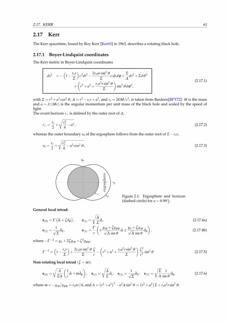
2.17. KERR 61
2.17 Kerr
The Kerr spacetime, found by Roy Kerr [Ker63] in 1963, describes a rotating black hole.
2.17.1 Boyer-Lindquist coordinates
The Kerr metric in Boyer-Lindquist coordinates
ds2 =−(
1− rsrΣ
)c2dt2− 2rsar sin2
ϑ
Σcdt dϕ +
Σ
∆dr2 +Σdϑ
2
+
(r2 +a2 +
rsa2r sin2ϑ
Σ
)sin2
ϑdϕ2,
(2.17.1)
with Σ = r2 +a2 cos2 ϑ , ∆ = r2− rsr+a2, and rs = 2GM/c2, is taken from Bardeen[BPT72]. M is the massand a = J/(Mc) is the angular momentum per unit mass of the black hole and scaled by the speed oflight.The event horizon r+ is defined by the outer root of ∆ ,
r+ =rs
2+
√r2
s
4−a2, (2.17.2)
whereas the outer boundary r0 of the ergosphere follows from the outer root of Σ − rsr,
r0 =rs
2+
√r2
s
4−a2 cos2 ϑ , (2.17.3)
x
y
ergosphere
r+r0 Figure 2.1: Ergosphere and horizon
(dashed circle) for a = 0.99 rs2 .
General local tetrad:
e(0) = Γ(∂t +ζ ∂ϕ
), e(1) =
√∆
Σ∂r, (2.17.4a)
e(2) =1√Σ
∂ϑ , e(3) =Γ
c
(∓gtϕ +ζ gϕϕ√
∆ sinϑ∂t ±
gtt +ζ gtϕ√∆ sinϑ
∂ϕ
), (2.17.4b)
where −Γ−2 = gtt +2ζ gtϕ +ζ 2gϕϕ ,
Γ−2 =
(1− rsr
Σ
)+
2rsar sin2ϑ
Σ
ζ
c−(
r2 +a2 +rsa2r sin2
ϑ
Σ
)ζ 2
c2 sin2ϑ (2.17.5)
Non-rotating local tetrad (ζ = ω):
e(0) =√
AΣ∆
(1c
∂t +ω∂ϕ
), e(1) =
√∆
Σ∂r, e(2) =
1√Σ
∂ϑ , e(3) =√
Σ
A1
sinϑ∂ϕ , (2.17.6)
where ω =−gtϕ/gϕϕ = rsar/A, and A =(r2 +a2
)2−a2∆ sin2ϑ =
(r2 +a2
)Σ + rsa2r sin2
ϑ .
62 CHAPTER 2. SPACETIMES
Dual tetrad:
θ(2) =
√Σ∆
Acdt, θ(1) =
√Σ
∆dr, θ(2) =
√Σdϑ , θ(3) =
√AΣ
sinϑ (dϕ−ω dϕ) . (2.17.7)
The relation between the constants of motion E, L, Q, and µ (defined in Bardeen[BPT72]) and the initialdirection υ, compare Sec. (1.4.5), with respect to the LNRF reads (c = 1)
υ(0) =
√A
Σ∆E− rsra√
AΣ∆L, υ
(1) =
√∆
Σpr, (2.17.8a)
υ(2) =
1√Σ
√Q− cos2 ϑ
[a2 (µ2−E2)+
L2
sin2ϑ
], υ
(3) =
√Σ
AL
sinϑ. (2.17.8b)
Static local tetrad (ζ = 0):
e(0) =1
c√
1− rsr/Σ∂t , e(1) =
√∆
Σ∂r, e(2) =
1√Σ
∂ϑ , (2.17.9a)
e(3) =±rsar sinϑ
c√
1− rsr/Σ√
∆Σ∂t ∓
√1− rsr/Σ√∆ sinϑ
∂ϕ . (2.17.9b)
Christoffel symbols:
Γr
tt =c2rs∆(r2−a2 cos2 ϑ)
2Σ 3 , Γϑ
tt =−c2rsa2r sinϑ cosϑ
Σ 3 , (2.17.10a)
Γt
tr =rs(r2 +a2)(r2−a2 cos2 ϑ)
2Σ 2∆, Γ
ϕ
tr =crsa(r2−a2 cos2 ϑ)
2Σ 2∆, (2.17.10b)
Γt
tϑ =− rsa2r sinϑ cosϑ
Σ 2 , Γϕ
tϑ =−crsar cotϑ
Σ 2 , (2.17.10c)
Γr
tϕ =−c∆rsasin2ϑ(r2−a2 cos2 ϑ)
2Σ 3 , Γϑ
tϕ =crsar(r2 +a2)sinϑ cosϑ
Σ 3 , (2.17.10d)
Γr
rr =2ra2 sin2
ϑ − rs(r2−a2 cos2 ϑ)
2Σ∆, Γ
ϑrr =
a2 sinϑ cosϑ
Σ∆, (2.17.10e)
Γr
rϑ =−a2 sinϑ cosϑ
Σ, Γ
ϑrϑ =
rΣ, (2.17.10f)
Γr
ϑϑ =− r∆
Σ, Γ
ϑϑϑ =−a2 sinϑ cosϑ
Σ, (2.17.10g)
Γϕ
ϑϕ=
cotϑ
Σ 2
[Σ
2 + rsa2r sin2ϑ], Γ
tϑϕ =
rsa3r sin3ϑ cosϑ
cΣ 2 , (2.17.10h)
Γt
rϕ =rsasin2
ϑ[a2 cos2 ϑ(a2− r2)− r2(a2 +3r2)
]2cΣ 2∆
, (2.17.10i)
Γϕ
rϕ =2rΣ 2 + rs
[a4 sin2
ϑ cos2 ϑ − r2(Σ + r2 +a2)]
2Σ 2∆, (2.17.10j)
Γr
ϕϕ =∆ sin2
ϑ
2Σ 3
[−2rΣ
2 + rsa2 sin2ϑ(r2−a2 cos2
ϑ)], (2.17.10k)
Γϑ
ϕϕ =− sinϑ cosϑ
Σ 3
[AΣ +
(r2 +a2)rsa2r sin2
ϑ], (2.17.10l)
Photon orbits:The direct(-) and retrograd(+) photon orbits have radius
rpo = rs
[1+ cos
(23
arccos∓2a
rs
)]. (2.17.11)
2.17. KERR 63
Marginally stable timelike circular orbitsare defined via
rms =rs
2
(3+Z2∓
√(3−Z1)(2+Z1 +2Z2)
), (2.17.12)
where
Z1 = 1+(
1− 4a2
r2s
)1/3[(
1+2ars
)1/3
+
(1− 2a
rs
)1/3], (2.17.13a)
Z2 =
√12a2
r2s
+Z21 . (2.17.13b)
Euler-Lagrange:The Euler-Lagrangian formalism, Sec. 1.8.4, for geodesics in the ϑ = π/2 hyperplane yields
12
r2 +Veff = 0 (2.17.14)
with the effective potential
Veff =1
2r3
h2(r− rs)+2
ahkc
rs−k2
c2
[r3 +a2(r+ rs)
]− κc2∆
r2 (2.17.15)
and the constants of motion
k =(
1− rs
r
)c2t +
crsar
ϕ, h =
(r2 +a2 +
rsa2
r
)ϕ− crsa
rt. (2.17.16)
Timelike circular orbitsA timelike circular geodesic, see Sec. 1.9.1, is given by
β1,2 =rsar4
(3r2 +a2
)±A√
2r7rs
r2√
∆ (−2r5 + rsa2r2), (2.17.17)
where the positive sign is for contrarotating and the negative sign for corotating orbits, and β1,2 are w.r.t.the LNRF.Further reading:Boyer and Lindquist[BL67], Wilkins[Wil72], Brill[BC66].
64 CHAPTER 2. SPACETIMES
2.18 Kottler spacetime
The Kottler spacetime is represented in spherical coordinates (t,r,ϑ ,ϕ) by the line element[Per04]
ds2 =−(
1− rs
r− Λr2
3
)c2dt2 +
11− rs/r−Λr2/3
dr2 + r2dΩ2, (2.18.1)
where rs = 2GM/c2 is the Schwarzschild radius, G is Newton’s constant, c is the speed of light, M isthe mass of the black hole, and Λ is the cosmological constant. If Λ > 0 the metric is also known asSchwarzschild-deSitter metric, whereas if Λ < 0 it is called Schwarzschild-anti-deSitter.For the following, we define the two abbreviations
α = 1− rs
r− Λr2
3and β =
rs
r− 2Λ
3r2. (2.18.2)
The critical points of the Kottler metric follow from the roots of the cubic equation α = 0. These can befound by means of the parameters p =−1/Λ and q = 3rs/(2Λ). If Λ < 0, we have only one real root
r1 =2√−Λ
sinh[
13
arsinh(
3rs
2
√−Λ
)]. (2.18.3)
If Λ > 0, we have to distinguish whether D≡ q2 + p3 = 9r2s /(4Λ 2)−Λ−3 is positive or negative. If D > 0,
there is no real positive root. For D < 0, the two real positive roots read
r± =2√Λ
cos[
π
3± 1
3arccos
(3rs
2
√Λ
)](2.18.4)
Christoffel symbols:
Γr
tt =c2αβ
2r, Γ
ttr =
β
2rα, Γ
rrr =−
β
2rα, (2.18.5a)
Γϑ
rϑ =1r, Γ
ϕ
rϕ =1r, Γ
rϑϑ =−αr, (2.18.5b)
Γϕ
ϑϕ= cotϑ , Γ
rϕϕ =−αr sin2
ϑ , Γϑ
ϕϕ =−sinϑ cosϑ . (2.18.5c)
Riemann-Tensor:
Rtrtr =−c2(3rs +Λr3
)3r3 , Rtϑ tϑ =
12
c2αβ , (2.18.6a)
Rtϕtϕ =12
c2αβ sin2
ϑ , Rrϑrϑ =− β
2α, (2.18.6b)
Rrϕrϕ =− β
2αsin2
ϑ , Rϑϕϑϕ = r(
rs +Λr3
3
)sin2
ϑ . (2.18.6c)
Ricci-Tensor:
Rtt =−c2αΛ , Rrr =
Λ
α, Rϑϑ = Λr2, Rϕϕ = Λr2 sin2
ϑ . (2.18.7)
The Ricci scalar and the Kretschmann scalar read
R = 4Λ , K = 12r2
s
r6 +8Λ 2
3. (2.18.8)
Weyl-Tensor:
Ctrtr =−c2rs
r3 , Ctϑ tϑ =c2αrs
2r, Ctϕtϕ =
c2αrs sin2ϑ
2r, (2.18.9a)
Crϑrϑ =− rs
2rα, Crϕrϕ =− rs sin2
ϑ
2rα, Cϑϕϑϕ = rrs sin2
ϑ . (2.18.9b)
2.18. KOTTLER SPACETIME 65
Local tetrad:
e(t) =1
c√
α∂t , e(r) =
√α∂r, e(ϑ) =
1r
∂ϑ , e(ϕ) =1
r sinϑ∂ϕ . (2.18.10)
Dual tetrad:
θ(t) = c√
α dt, θ(r) =dr√
α, θ(ϑ) = r dϑ , θ(ϕ) = r sinϑ dϕ. (2.18.11)
Ricci rotation coefficients:
γ(r)(t)(t) =rs− 2
3Λr3
2r2√
α, γ(ϑ)(r)(ϑ) = γ(ϕ)(r)(ϕ) =
√α
r, γ(ϕ)(ϑ)(ϕ) =
cotϑ
r. (2.18.12)
The contractions of the Ricci rotation coefficients read
γ(r) =4r−3rs−2Λr3
2r2√
α, γ(ϑ) =
cotϑ
r. (2.18.13)
Riemann-Tensor with respect to local tetrad:
R(t)(r)(t)(r) =−R(ϑ)(ϕ)(ϑ)(ϕ) =−Λr3 +3rs
3r3 , (2.18.14a)
R(t)(ϑ)(t)(ϑ) = R(t)(ϕ)(t)(ϕ) =−R(r)(ϑ)(r)(ϑ) =−R(r)(ϕ)(r)(ϕ) =3rs−2Λr3
6r3 . (2.18.14b)
Weyl-Tensor with respect to local tetrad:
C(t)(r)(t)(r) =−C(ϑ)(ϕ)(ϑ)(ϕ) =−rs
r3 , (2.18.15a)
C(t)(ϑ)(t)(ϑ) =C(t)(ϕ)(t)(ϕ) =−C(r)(ϑ)(r)(ϑ) =−C(r)(ϕ)(r)(ϕ) =rs
2r3 . (2.18.15b)
Embedding:The embedding function follows from the numerical integration of
dzdr
=
√rs/r+Λr2/3
1− rs/r−Λr2/3. (2.18.16)
Euler-Lagrange:The Euler-Lagrangian formalism[Rin01] yields the effective potential
Veff =12
(1− rs
r− Λr2
3
)(h2
r2 −κc2)
(2.18.17)
with the constants of motion k = (1− rs/r−Λr2/3)c2t, h = r2ϕ , and κ as in Eq. (1.8.2).As in the Schwarzschild metric, the effective potential has only one extremum for null geodesics, the socalled photon orbit at r = 3
2 rs. For timelike geodesics, however, we have
dVeff
dr=
h2(−6r+9rs)+ c2r2(3rs−2r3Λ)
3r4!= 0. (2.18.18)
This polynomial of fifth order might have up to five extrema.
Further reading:Kottler[Kot18], Weyl[Wey19], Hackmann[HL08], Cruz[COV05].
66 CHAPTER 2. SPACETIMES
2.19 Majumdar-Papapetrou spacetimes
The Majumdar-Papapetrou (MP) metric[Cha89] describes an ensemble of N extreme Reissner-Nordstrøm(RN) black holes (see 2.25.3) with masses Mk at locations rk (k = 1,2, ...,N) and charges of the same sign.Because of the charge-mass ratio of each black hole, their gravitational attraction is exactly compensatedby their electrostatic repulsion. In Cartesian coordinates t,x,y,z ∈ R the MP metric reads
ds2 =−c2dt2
U2 +U2(dx2 +dy2 +dz2), (2.19.1)
where
U(x,y,z) = 1+N
∑k=1
Rk/2|r−rk|
(2.19.2)
with Rk = 2GMk/c2 and r = (x,y,z)T . The coordinate singularity rk is the degenerated horizon of the k-thextreme RN black hole. For N = 2, the MP spacetime is called extreme RN dihole metric (see 2.10.1).
Derivations of U(x,y,z):
∂xU =N
∑k=1
Rk
2xk− x|r−rk|3
, ∂2x U =
N
∑k=1
Rk
23(x− xk)
2−|r−rk|2|r−rk|5
, (2.19.3a)
∂yU =N
∑k=1
Rk
2yk− y|r−rk|3
, ∂2y U =
N
∑k=1
Rk
23(y− yk)
2−|r−rk|2|r−rk|5
, (2.19.3b)
∂zU =N
∑k=1
Rk
2zk− z|r−rk|3
, ∂2z U =
N
∑k=1
Rk
23(z− zk)
2−|r−rk|2|r−rk|5
, (2.19.3c)
∂x∂yU =N
∑k=1
3Rk
2(xk− x)(yk− y)|r−rk|5
, ∂x∂zU =N
∑k=1
3Rk
2(xk− x)(zk− z)|r−rk|5
, (2.19.3d)
∂y∂zU =N
∑k=1
3Rk
2(yk− y)(zk− z)|r−rk|5
. (2.19.3e)
The function U(x,y,z) fulfills the Laplace-Equation ∆U = 0, which will be used in the calculation of thefollowing geometric quantities.
Christoffel symbols:
Γx
tt =−c2∂xU
U5 , Γy
tt =−c2∂yU
U5 , Γz
tt =−c2∂zU
U5 , Γt
tx =−∂xUU
, (2.19.4a)
Γx
xx =∂xUU
, Γy
xx =−∂yUU
, Γz
xx =−∂zUU
, Γt
ty =−∂yUU
, (2.19.4b)
Γx
xy =∂yUU
, Γy
xy =∂xUU
, Γx
yy =−∂xUU
, Γy
yy =∂yUU
, (2.19.4c)
Γz
yy =−∂zUU
, Γt
tz =−∂zUU
, Γx
xz =∂zUU
, Γz
xz =∂xUU
, (2.19.4d)
Γy
yz =∂zUU
, Γz
yz =∂yUU
, Γx
zz =−∂xUU
, Γy
zz =−∂yUU
, (2.19.4e)
Γz
zz =∂zUU
. (2.19.4f)
2.19. MAJUMDAR-PAPAPETROU SPACETIMES 67
Riemann-Tensor:
Rtxtx =c2
U4
[4(∂xU)2−U∂
2x U− (∇U)2] , Rxyxz = 2∂yU∂zU−U∂y∂zU, (2.19.5a)
Rtyty =c2
U4
[4(∂yU)2−U∂
2y U− (∇U)2] , Rxzxy = 2∂yU∂zU−U∂y∂zU, (2.19.5b)
Rtztz =c2
U4
[4(∂zU)2−U∂
2z U− (∇U)2] , Rxzyz = 2∂xU∂yU−U∂x∂yU, (2.19.5c)
Rtxty =c2
U4 (4∂xU∂yU−U∂x∂yU) , Rxyxy = (∇U)2−2(∂zU)2 +U∂2z U, (2.19.5d)
Rtytx =c2
U4 (4∂xU∂yU−U∂x∂yU) , Rxzxz = (∇U)2−2(∂yU)2 +U∂2y U, (2.19.5e)
Rtztx =c2
U4 (4∂xU∂zU−U∂x∂zU) , Ryzyz = (∇U)2−2(∂xU)2 +U∂2x U, (2.19.5f)
Rtxtz =c2
U4 (4∂xU∂zU−U∂x∂zU) , Ryzxz = 2∂xU∂yU−U∂x∂yU, (2.19.5g)
Rtytz =c2
U4 (4∂yU∂zU−U∂y∂zU) , Rxyyz =−2∂xU∂zU +U∂x∂zU, (2.19.5h)
Rtzty =c2
U4 (4∂yU∂zU−U∂y∂zU) , Ryzxy =−2∂xU∂zU +U∂x∂zU. (2.19.5i)
Ricci-Tensor:
Rxx =(∇U)2−2(∂xU)2
U2 , Rtt =c2
U6 (∇U)2, Rxy =−2∂xU∂yU
U2 , (2.19.6a)
Ryy =(∇U)2−2(∂yU)2
U2 , Rxz =−2∂xU∂zU
U2 , Ryz =−2∂yU∂zU
U2 , (2.19.6b)
Rzz =(∇U)2−2(∂zU)2
U2 . (2.19.6c)
The Ricci scalar vanishes identically, also because the energy-momentum tensor of the electromagneticfield is traceless. The Kretschmann scalar reads
K =4
U8
14(∂zU)4 +14
[(∂yU)2 +(∂xU)2]2−24U∂zU (∂yU∂y∂zU +∂xU∂x∂zU)
−12U((∂xU)2
∂2x U +2∂xU∂yU∂x∂yU +(∂yU)2
∂2y U)
+U2((∂ 2
z U)2 +4(∂y∂zU)2 +3(∂ 2y U)2 +4(∂x∂zU)2 +4(∂x∂yU)2
+2∂2y U∂
2x U +3(∂ 2
x U)2)
+4(∂zU)2(
7[(∂yU)2 +(∂xU)2]−3U∂
2z U)
.
(2.19.7)
68 CHAPTER 2. SPACETIMES
Weyl-Tensor:
Ctxtx =c2
U4
[3(∂xU)2−U∂
2x U− (∇U)2] , Cxyxz = 3∂yU∂zU−U∂y∂zU, (2.19.8a)
Ctyty =c2
U4
[3(∂yU)2−U∂
2y U− (∇U)2] , Cxzxy = 3∂yU∂zU−U∂y∂zU, (2.19.8b)
Ctztz =c2
U4
[3(∂zU)2−U∂
2z U− (∇U)2] , Cxzyz = 3∂xU∂yU−U∂x∂yU, (2.19.8c)
Ctxty =c2
U4 (3∂xU∂yU−U∂x∂yU) , Cxyxy = (∇U)2−3(∂zU)2 +U∂2z U, (2.19.8d)
Ctytx =c2
U4 (3∂xU∂yU−U∂x∂yU) , Cxzxz = (∇U)2−3(∂yU)2 +U∂2y U, (2.19.8e)
Ctztx =c2
U4 (3∂xU∂zU−U∂x∂zU) , Cyzyz = (∇U)2−3(∂xU)2 +U∂2x U, (2.19.8f)
Ctxtz =c2
U4 (3∂xU∂zU−U∂x∂zU) , Cyzxy =−3∂xU∂zU +U∂x∂zU, (2.19.8g)
Ctytz =c2
U4 (3∂yU∂zU−U∂y∂zU) , Cxyyz =−3∂xU∂zU +U∂x∂zU, (2.19.8h)
Ctzty =c2
U4 (3∂yU∂zU−U∂y∂zU) , Cyzxz = 3∂xU∂yU−U∂x∂yU. (2.19.8i)
Local tetrad:
e(t) =Uc
∂t , e(x) =1U
∂x, e(y) =1U
∂y, e(z) =1U
∂z. (2.19.9)
Dual tetrad:
θ(t) =cU
dt, θ(x) =Udx, θ(y) =Udy, θ(z) =Udz. (2.19.10)
Ricci rotation coefficients:
γ(t)(x)(t) = γ(y)(x)(y) = γ(z)(x)(z) =∂xUU2 , γ(t)(y)(t) = γ(x)(y)(x) = γ(z)(y)(z) =
∂yUU2 , (2.19.11a)
γ(t)(z)(t) = γ(x)(z)(x) = γ(y)(z)(y) =∂zUU2 . (2.19.11b)
The contractions of the Ricci rotation coefficients read
γ(x) =∂xUU2 , γ(y) =
∂yUU2 , γ(z) =
∂zUU2 . (2.19.12)
2.19. MAJUMDAR-PAPAPETROU SPACETIMES 69
Riemann-Tensor with respect to local tetrad:
R(t)(x)(t)(x) =1
U4
[4(∂xU)2−U∂
2x U− (∇U)2] , R(x)(y)(x)(z) =
1U4 (2∂yU∂zU−U∂y∂zU) , (2.19.13a)
R(t)(y)(t)(y) =1
U4
[4(∂yU)2−U∂
2y U− (∇U)2] , R(x)(z)(x)(y) =
1U4 (2∂yU∂zU−U∂y∂zU) , (2.19.13b)
R(t)(z)(t)(z) =1
U4
[4(∂zU)2−U∂
2z U− (∇U)2] , R(x)(z)(y)(z) =
1U4 (2∂xU∂yU−U∂x∂yU) , (2.19.13c)
R(x)(y)(x)(y) =1
U4
[(∇U)2−2(∂zU)2 +U∂
2z U], R(t)(x)(t)(y) =
1U4 (4∂xU∂yU−U∂x∂yU) , (2.19.13d)
R(x)(z)(x)(z) =1
U4
[(∇U)2−2(∂yU)2 +U∂
2y U], R(t)(y)(t)(x) =
1U4 (4∂xU∂yU−U∂x∂yU) , (2.19.13e)
R(y)(z)(y)(z) =1
U4
[(∇U)2−2(∂xU)2 +U∂
2x U], R(t)(z)(t)(x) =
1U4 (4∂xU∂zU−U∂x∂zU) , (2.19.13f)
R(t)(x)(t)(z) =1
U4 (4∂xU∂zU−U∂x∂zU) , R(y)(z)(x)(z) =1
U4 (2∂xU∂yU−U∂x∂yU) , (2.19.13g)
R(t)(y)(t)(z) =1
U4 (4∂yU∂zU−U∂y∂zU) , R(x)(y)(y)(z) =1
U4 (−2∂xU∂zU +U∂x∂zU) , (2.19.13h)
R(t)(z)(t)(y) =1
U4 (4∂yU∂zU−U∂y∂zU) , R(y)(z)(x)(y) =1
U4 (−2∂xU∂zU +U∂x∂zU) . (2.19.13i)
Ricci-Tensor with respect to local tetrad:
R(x)(x) =(∇U)2−2(∂xU)2
U4 , R(t)(t) =(∇U)2
U4 , R(x)(y) =−2∂xU∂yU
U4 , (2.19.14a)
R(y)(y) =(∇U)2−2(∂yU)2
U4 , R(x)(z) =−2∂xU∂zU
U4 , R(y)(z) =−2∂yU∂zU
U4 , (2.19.14b)
R(z)(z) =(∇U)2−2(∂zU)2
U4 . (2.19.14c)
Weyl-Tensor with respect to local tetrad:
C(t)(x)(t)(x) =1
U4
[3(∂xU)2−U∂
2x U− (∇U)2] , C(x)(y)(x)(z) =
1U4 (3∂yU∂zU−U∂y∂zU) , (2.19.15a)
C(t)(y)(t)(y) =1
U4
[3(∂yU)2−U∂
2y U− (∇U)2] , C(x)(z)(x)(y) =
1U4 (3∂yU∂zU−U∂y∂zU) , (2.19.15b)
C(t)(z)(t)(z) =1
U4
[3(∂zU)2−U∂
2z U− (∇U)2] , C(x)(z)(y)(z) =
1U4 (3∂xU∂yU−U∂x∂yU) , (2.19.15c)
C(x)(y)(x)(y) =1
U4
[(∇U)2−3(∂zU)2 +U∂
2z U], C(t)(x)(t)(y) =
1U4 (3∂xU∂yU−U∂x∂yU) , (2.19.15d)
C(x)(z)(x)(z) =1
U4
[(∇U)2−3(∂yU)2 +U∂
2y U], C(t)(y)(t)(x) =
1U4 (3∂xU∂yU−U∂x∂yU) , (2.19.15e)
C(y)(z)(y)(z) =1
U4
[(∇U)2−3(∂xU)2 +U∂
2x U], C(t)(z)(t)(x) =
1U4 (3∂xU∂zU−U∂x∂zU) , (2.19.15f)
C(t)(x)(t)(z) =1
U4 (3∂xU∂zU−U∂x∂zU) , C(y)(z)(x)(y) =1
U4 (−3∂xU∂zU +U∂x∂zU) , (2.19.15g)
C(t)(y)(t)(z) =1
U4 (3∂yU∂zU−U∂y∂zU) , C(x)(y)(y)(z) =1
U4 (−3∂xU∂zU +U∂x∂zU) , (2.19.15h)
C(t)(z)(t)(y) =1
U4 (3∂yU∂zU−U∂y∂zU) , C(y)(z)(x)(z) =1
U4 (3∂xU∂yU−U∂x∂yU) . (2.19.15i)
Further reading:Chandrasekhar[Cha89, Cha06], Hartle[HH72], Yurtsever[Yur95], Wünsch[WMW13],
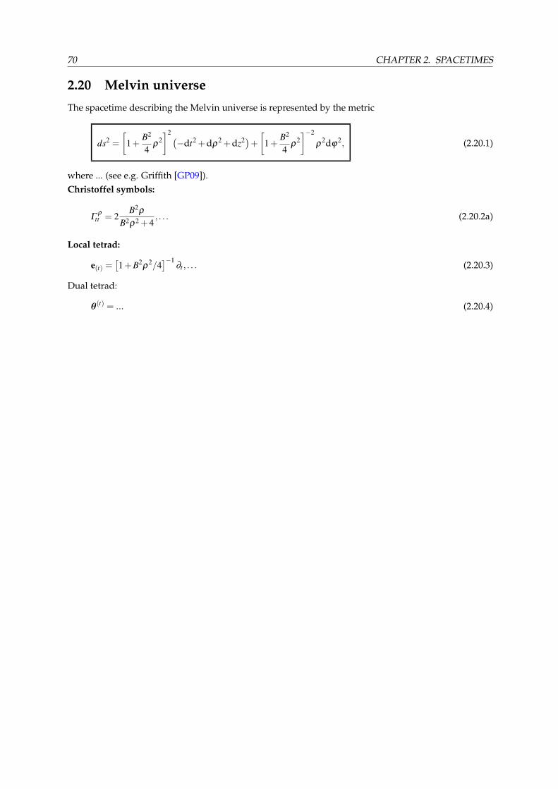
70 CHAPTER 2. SPACETIMES
2.20 Melvin universe
The spacetime describing the Melvin universe is represented by the metric
ds2 =
[1+
B2
4ρ
2]2 (−dt2 +dρ
2 +dz2)+[1+B2
4ρ
2]−2
ρ2dϕ
2, (2.20.1)
where ... (see e.g. Griffith [GP09]).Christoffel symbols:
Γρ
tt = 2B2ρ
B2ρ2 +4, . . . (2.20.2a)
Local tetrad:
e(t) =[1+B2
ρ2/4]−1
∂t , . . . (2.20.3)
Dual tetrad:
θ(t) = ... (2.20.4)
2.21. MORRIS-THORNE 71
2.21 Morris-Thorne
The most simple wormhole geometry is represented by the metric of Morris and Thorne[MT88],
ds2 =−c2dt2 +dl2 +(b20 + l2)
(dϑ
2 + sin2ϑ dϕ
2) , (2.21.1)
where b0 is the throat radius and l is the proper radial coordinate; and t ∈R, l ∈R,ϑ ∈ (0,π),ϕ ∈ [0,2π).Christoffel symbols:
Γϑ
lϑ =l
b20 + l2 , Γ
ϕ
lϕ =l
b20 + l2 , Γ
lϑϑ =−l, (2.21.2a)
Γϕ
ϑϕ= cotϑ , Γ
lϕϕ =−l sin2
ϑ , Γϑ
ϕϕ =−sinϑ cosϑ . (2.21.2b)
Partial derivatives
Γϑ
lϑ ,l =−l2−b2
0
(b20 + l2)2 , Γ
ϕ
lϕ,l =−l2−b2
0
(b20 + l2)2 , Γ
lϑϑ ,l =−1, (2.21.3a)
Γϕ
ϑϕ,ϑ =− 1sin2
ϑ, Γ
lϕϕ,l =−sin2
ϑ , Γl
ϕϕ,ϑ =−l sin(2ϑ), (2.21.3b)
Γϑ
ϕϕ,ϑ =−cos(2ϑ). (2.21.3c)
Riemann-Tensor:
Rlϑ lϑ =− b20
b20 + l2 , Rlϕlϕ =−b2
0 sin2ϑ
b20 + l2 , Rϑϕϑϕ = b2
0 sin2ϑ . (2.21.4)
Ricci tensor, Ricci and Kretschmann scalar:
Rll =−2b2
0(b2
0 + l2)2 , R =−2
b20(
b20 + l2
)2 , K =12b4
0(b2
0 + l2)4 . (2.21.5)
Weyl-Tensor:
Ctltl =−23
c2b20(
b20 + l2
)2 , Ctϑ tϑ =13
c2b20
b20 + l2 , Ctϕtϕ =
13
c2b20 sin2
ϑ
b20 + l2 , (2.21.6a)
Clϑ lϑ =−13
b20
b20 + l2 , Clϕlϕ =−1
3b2
0 sin2ϑ
b20 + l2 , Cϑϕϑϕ =
23
b20 sin2
ϑ . (2.21.6b)
Local tetrad:
e(t) =1c
∂t , e(l) = ∂l , e(ϑ) =1√
b20 + l2
∂ϑ , e(ϕ) =1√
b20 + l2 sinϑ
∂ϕ . (2.21.7)
Dual tetrad
θ(t) = cdt, θ(l) = dl, θ(ϑ) =√
b20 + l2 dϑ , θ(ϕ) =
√b2
0 + l2 sinϑ dϕ. (2.21.8)
Ricci rotation coefficients:
γ(ϑ)(l)(ϑ) = γ(ϕ)(l)(ϕ) =l
b20 + l2 , γ(ϕ)(ϑ)(ϕ) =
cotϑ√b2
0 + l2. (2.21.9)
The contractions of the Ricci rotation coefficients read
γ(l) =2l
b20 + l2 , γ(ϑ) =
cotϑ√b2
0 + l2. (2.21.10)
72 CHAPTER 2. SPACETIMES
Riemann-Tensor with respect to local tetrad:
R(l)(ϑ)(l)(ϑ) = R(l)(ϕ)(l)(ϕ) =−R(ϑ)(ϕ)(ϑ)(ϕ) =−b2
0(b2
0 + l2)2 . (2.21.11)
Ricci-Tensor with respect to local tetrad:
R(l)(l) =−2b2
0(b2
0 + l2)2 . (2.21.12)
Weyl-Tensor with respect to local tetrad:
C(t)(l)(t)(l) =−C(ϑ)(ϕ)(ϑ)(ϕ) =−2b2
0
3(b2
0 + l2)2 , (2.21.13a)
C(t)(ϑ)(t)(ϑ) =C(t)(ϕ)(t)(ϕ) =−C(l)(ϑ)(l)(ϑ) =−C(l)(ϕ)(l)(ϕ) =b2
0
3(b2
0 + l2)2 . (2.21.13b)
Embedding:The embedding function reads
z(r) =±b0 ln
rb0
+
√(r
b0
)2
−1
(2.21.14)
with r2 = b20 + l2.
Euler-Lagrange:The Euler-Lagrangian formalism, Sec. 1.8.4, for geodesics in the ϑ = π/2 hyperplane yields
12
l2 +Veff =12
k2
c2 , Veff =12
(h2
b20 + l2 −κc2
), (2.21.15)
with the constants of motion k = c2t and h = (b20 + l2)ϕ . The shape of the effective potential Veff is inde-
pendend of the geodesic type. The maximum of the effective potential is located at l = 0.
A geodesic that starts at l = li with direction y = ±e(t) + cosξ e(l) + sinξ e(ϕ) approaches the wormholethroat asymptotically for ξ = ξcrit with
ξcrit = arcsinb0√
b20 + l2
i
. (2.21.16)
This critical angle is independent of the type of the geodesic.
Further reading:Ellis[Ell73], Visser[Vis95], Müller[Mül04, Mül08a]
2.22. OPPENHEIMER-SNYDER COLLAPSE 73
2.22 Oppenheimer-Snyder collapse
2.22.1 Outer metric
The metric of the outer spacetime, R > Rb, in comoving coordinates (τ,R,ϑ ,ϕ) with (c = 1) is given by
ds2 =−dτ2 +
R(R3/2− 3
2√
rsτ)2/3 dR2 +
(R3/2− 3
2√
rsτ
)4/3 (dϑ
2 + sin2ϑdϕ
2) . (2.22.1)
Christoffel symbols:
ΓR
τR =12
√rs
R3/2− 32√
rsτ, Γ
ϑτϑ =−
√rs
R3/2− 32√
rsτ, (2.22.2a)
Γϕ
τϕ =−√
rs
R3/2− 32√
rsτ, Γ
τRR =
R√
rs
2(R3/2− 3
2√
rsτ)5/3 , (2.22.2b)
ΓR
RR =− 3√
rsτ
4(R3/2− 3
2√
rsτ)
R, Γ
ϑRϑ =
√R
R3/2− 32√
rsτ, (2.22.2c)
Γϕ
Rϕ=
√R
R3/2− 32√
rsτ, Γ
τϑϑ =−√rs
(R3/2− 3
2√
rsτ
)1/3
, (2.22.2d)
ΓR
ϑϑ =−R3/2− 32√
rsτ√R
, Γϕ
ϑϕ= cotϑ , (2.22.2e)
Γτ
ϕϕ =−√rs
(R3/2− 3
2√
rsτ
)1/3
sin2ϑ , Γ
ϑϕϕ =−sinϑ cosϑ , (2.22.2f)
ΓR
ϕϕ =−(R3/2− 3
2√
rsτ)
sin2ϑ√
R. (2.22.2g)
Riemann-Tensor:
RτRτR =− Rrs(R3/2− 3
2√
rs τ)8/3 , Rτϑτϑ =
12
rs(R3/2− 3
2√
rs τ)2/3 , (2.22.3a)
Rτϕτϕ =12
rs sin2ϑ(
R3/2− 32√
rs τ)2/3 , RRϑRϑ =−1
2Rrs(
R3/2− 32√
rs τ)4/3 , (2.22.3b)
RRϕRϕ =−12
Rrs sin2ϑ(
R3/2− 32√
rs τ)4/3 , Rϑϕϑϕ =
(R3/2− 3
2√
rs τ
)2/3
rs sin2ϑ . (2.22.3c)
The Ricci tensor and the Ricci scalar vanish identically.Kretschmann scalar:
K = 12r2
s(R3/2− 3
2√
rs τ)4 . (2.22.4)
Local tetrad:
e(τ) = ∂τ , e(R) =(R3/2− 3
2√
rsτ)1/3
√R
∂R, (2.22.5a)
e(ϑ) =1(
R3/2− 32√
rsτ)2/3 ∂ϑ , e(ϕ) =
1(R3/2− 3
2√
rsτ)2/3
sinϑ
∂ϕ . (2.22.5b)
74 CHAPTER 2. SPACETIMES
Ricci rotation coefficients:
γ(τ)(R)(R) =−√
rs
2R3/2−3√
rsτ, γ(τ)(ϑ)(ϑ) = γ(τ)(ϕ)(ϕ) =
2√
rs
2R3/2−3√
rsτ, (2.22.6a)
γ(R)(ϕ)(ϕ) = γ(R)(ϑ)(ϑ) =−(
R3/2− 32√
rsτ
)−2/3
. (2.22.6b)
The contractions of the Ricci rotation coefficients read
γ(τ) =−3√
rs
2R3/2−3√
rsτ, γ(R) = 2
(R3/2− 3
2√
rsτ
)−2/3
, γ(ϑ) = cotϑ
(R3/2− 3
2√
rsτ
)−2/3
. (2.22.7)
Riemann-Tensor with respect to local tetrad:
R(τ)(R)(τ)(R) =−R(ϑ)(ϕ)(ϑ)(ϕ) =−4rs(
2R3/2−3√
rsτ)2 , (2.22.8a)
R(τ)(ϑ)(τ)(ϑ) = R(τ)(ϕ)(τ)(ϕ) =−R(R)(ϑ)(R)(ϑ) =−R(R)(ϕ)(R)(ϕ) =2rs(
2R3/2−3√
rsτ)2 . (2.22.8b)
The Ricci tensor with respect to the local tetrad vanishes identically.
2.22.2 Inner metric
The metric of the inside, R≤ Rb, reads
ds2 =−dτ2 +
(1− 3
2√
rsR−3/2b τ
)4/3 [dR2 +R2 (dϑ
2 + sin2ϑdϕ
2)] . (2.22.9)
For the following components, we define
AOin := 1− 32√
rsR−3/2b τ. (2.22.10)
Christoffel symbols:
ΓR
τR =−√
rsR−3/2b
AOin, Γ
ϑτϑ =−
√rsR−3/2b
AOin, Γ
ϕ
τϕ =−√
rsR−3/2b
AOin, (2.22.11a)
Γτ
RR =−A1/3Oin√
rsR−3/2b , Γ
ϑRϑ =
1R, Γ
ϕ
Rϕ=
1R, (2.22.11b)
ΓR
ϑϑ =−R, Γϕ
ϑϕ= cotϑ , Γ
τϑϑ =−A1/3
Oin√
rsR−3/2b R2, (2.22.11c)
ΓR
ϕϕ =−Rsin2ϑ , Γ
ϑϕϕ =−sinϑ cosϑ , Γ
τϕϕ =−A1/3
Oin√
rsR−3/2b R2 sin2
ϑ . (2.22.11d)
Riemann-Tensor:
RτRτR =12
rs
R3bA2/3
Oin
, Rτϑτϑ =12
rsR2
R3bA2/3
Oin
, Rτϕτϕ =12
rsR2 sin2ϑ
R3bA2/3
Oin
, (2.22.12a)
RRϕRϕ =rsR2 sin2
ϑ
R3b
A2/3Oin, RRϑRϑ =
rsR2
R3b
A2/3Oin, Rϑϕϑϕ =
rsR4 sin2ϑ
R3b
A2/3Oin. (2.22.12b)
Ricci-Tensor:
Rττ =32
rs
R3bA2
Oin, RRR =
32
rs
R3bA2/3
Oin
, Rϑϑ =32
rsR2
R3bA2/3
Oin
, Rϕϕ =32
rsR2 sin2ϑ
R3bA2/3
Oin
. (2.22.13)
2.22. OPPENHEIMER-SNYDER COLLAPSE 75
The Ricci and Kretschmann scalars read:
R =3rs
R3bA2
Oin, K = 15
r2s
R6bA4
Oin. (2.22.14)
Local tetrad:
e(τ) = ∂τ , e(R) =1
A2/3Oin
∂R, e(ϑ) =1
RA2/3Oin
∂ϑ , e(ϕ) =1
A2/3OinRsinϑ
∂ϕ . (2.22.15)
Ricci rotation coefficients:
γ(τ)(R)(R) = γ(τ)(ϑ)(ϑ) = γ(τ)(ϕ)(ϕ) =
√rsR−3/2b
AOin, (2.22.16a)
γ(R)(ϑ)(ϑ) = γ(R)(ϕ)(ϕ) =−1
RA2/3Oin
, (2.22.16b)
γ(ϑ)(ϕ)(ϕ) =−cotϑ
RA2/3Oin
. (2.22.16c)
The contractions of the Ricci rotation coefficients read
γ(τ) =−3√
rsR−3/2b
AOin, γ(R) =
2
RA2/3Oin
, γ(ϑ) =cotϑ
RA2/3Oin
. (2.22.17)
Riemann-Tensor with respect to local tetrad:
R(τ)(R)(τ)(R) = R(τ)(ϑ)(τ)(ϑ) = R(τ)(ϕ)(τ)(ϕ) =rsR−3
b
2A2Oin
, (2.22.18a)
R(R)(ϑ)(R)(ϑ) = R(R)(ϕ)(R)(ϕ) = R(ϑ)(ϕ)(ϑ)(ϕ) =rsR−3
b
A2Oin
. (2.22.18b)
Ricci-Tensor with respect to local tetrad:
R(τ)(τ) = R(R)(R) = R(ϑ)(ϑ) = R(ϕ)(ϕ) =3rsR−3
b
2A2Oin
. (2.22.19)
Further reading:Oppenheimer and Snyder[OS39].
76 CHAPTER 2. SPACETIMES
2.23 Petrov-Type D – Levi-Civita spacetimes
The Petrov type D static vacuum spacetimes AI-C are taken from Stephani et al.[SKM+03], Sec. 18.6,with the coordinate and parameter ranges given in "Exact solutions of the gravitational field equations"by Ehlers and Kundt [EK62].
2.23.1 Case AI
In spherical coordinates, (t,r,ϑ ,ϕ), the metric is given by the line element
ds2 = r2 (dϑ2 + sin2
ϑdϕ2)+ r
r−bdr2− r−b
rdt2. (2.23.1)
This is the well known Schwarzschild solution if b = rs, cf. Eq. (2.2.1). Coordinates and parameters arerestricted to
t ∈R, 0 < ϑ < π , ϕ ∈ [0,2π), (0 < b < r)∨ (b < 0 < r).
Local tetrad:
e(t) =√
rr−b
∂t , e(r) =√
r−br
∂r, e(ϑ) =1r
∂ϑ , e(ϕ) =1
r sinϑ∂ϕ . (2.23.2)
Dual tetrad:
θ(t) =
√r−b
rdt, θ(r) =
√r
r−bdr, θ(ϑ) = r dϑ , θ(ϕ) = r sinϑ dϕ. (2.23.3)
Effective potential:With the Hamilton-Jacobi formalism it is possible to obtain an effective potential fulfilling 1
2 r2+ 12Veff(r)=
12C2
0 with
Veff(r) = Kr−b
r3 −κr−b
r(2.23.4)
and the constants of motion
C20 = t2
(r−b
r
)2
, (2.23.5a)
K = ϑ2r4 + ϕ
2r4 sin2ϑ . (2.23.5b)
2.23.2 Case AII
In cylindrical coordinates, the metric is given by the line element
ds2 = z2 (dr2 + sinh2 r dϕ2)+ z
b− zdz2− b− z
zdt2. (2.23.6)
Coordinates and parameters are restricted to
t ∈R, 0 < r, ϕ ∈ [0,2π), 0 < z < b.
Local tetrad:
e(t) =√
zb− z
∂t , e(r) =1z
∂r, e(ϕ) =1
zsinhr∂ϕ , e(z) =
√b− z
z∂z. (2.23.7)
Dual tetrad:
θ(t) =
√b− z
zdt, θ(r) = zdr, θ(ϕ) = zsinhr dϕ, θ(z) =
√z
b− zdz. (2.23.8)
2.23. PETROV-TYPE D – LEVI-CIVITA SPACETIMES 77
2.23.3 Case AIII
In cylindrical coordinates, the metric is given by the line element
ds2 = z2 (dr2 + r2dϕ2)+ zdz2− 1
zdt2. (2.23.9)
Coordinates and parameters are restricted to
t ∈R, 0 < r, ϕ ∈ [0,2π), 0 < z.
Local tetrad:
e(t) =√
z∂t , e(r) =1z
∂r, e(ϕ) =1zr
∂ϕ , e(z) =1√z
∂z. (2.23.10)
Dual tetrad:
θ(t) =1√z
dt, θ(r) = zdr, θ(ϕ) = zr dϕ, θ(z) =√
zdz. (2.23.11)
2.23.4 Case BI
In spherical coordinates, the metric is given by the line element
ds2 = r2 (dϑ2− sin2
ϑdt2)+ rr−b
dr2 +r−b
rdϕ
2. (2.23.12)
Coordinates and parameters are restricted to
t ∈R, 0 < ϑ < π , ϕ ∈ [0,2π), (0 < b < r)∨ (b < 0 < r).
Local tetrad:
e(t) =1
r sinϑ∂t , e(r) =
√r−b
r∂r, e(ϑ) =
1r
∂ϑ , e(ϕ) =√
rr−b
∂ϕ . (2.23.13)
Dual tetrad:
θ(t) = r sinϑ dt, θ(r) =
√r
r−bdr, θ(ϑ) = r dϑ , θ(ϕ) =
√r−b
rdϕ. (2.23.14)
Effective potential:With the Hamilton-Jacobi formalism, an effective potential for the radial coordinate can be calculatedfulfilling 1
2 r2 + 12Veff(r) = 1
2C20 with
Veff(r) = Kr−b
r3 −κr−b
r(2.23.15)
and the constants of motion
C20 = ϕ
2(
r−br
)2
, (2.23.16a)
K = ϑ2r4− t2r4 sin2
ϑ . (2.23.16b)
Note that the metric is not spherically symmetric. Particles or light rays fall into one of the poles if theyare not moving in the ϑ = π
2 plane.
78 CHAPTER 2. SPACETIMES
2.23.5 Case BII
In cylindrical coordinates, the metric is given by the line element
ds2 = z2 (dr2− sinh2 r dt2)+ zb− z
dz2 +b− z
zdϕ
2. (2.23.17)
Coordinates and parameters are restricted to
t ∈R, ϕ ∈ [0,2π), 0 < z < b, 0 < r.
Local tetrad:
e(t) =1
zsinhr∂t , e(r) =
1z
∂r, e(ϕ) =√
zb− z
∂ϕ , e(z) =√
b− zz
∂z. (2.23.18)
Dual tetrad:
θ(t) = zsinhr dt, θ(r) = zdr, θ(ϕ) =
√b− z
zdϕ, θ(z) =
√z
b− zdz. (2.23.19)
2.23.6 Case BIII
In cylindrical coordinates, the metric is given by the line element
ds2 = z2 (dr2− r2dt2)+ zdz2 +1z
dϕ2. (2.23.20)
Coordinates and parameters are restricted to
t ∈R, ϕ ∈ [0,2π), 0 < z, 0 < r.
Local tetrad:
e(t) =1zr
∂t , e(r) =1z
∂r, e(ϕ) =√
z∂ϕ , e(z) =1√z
∂z. (2.23.21)
Dual tetrad:
θ(t) = zr dt, θ(r) = zdr, θ(ϕ) =1√z
dϕ, θ(z) =√
zdz. (2.23.22)
2.23.7 Case C
The metric is given by the line element
ds2 =1
(x+ y)2
(1
f (x)dx2 + f (x)dϕ
2− 1f (−y)
dy2 + f (−y)dt2)
(2.23.23)
with f (u) :=±(u3 +au+b). Coordinates and parameters are restricted to
0 < x+ y, f (−y)> 0, 0 > f (x).
Local tetrad:
e(t) = (x+ y)1√
−y3−ay+b∂t , e(x) = (x+ y)
√x3 +ax+b∂x, (2.23.24a)
e(y) = (x+ y)√−y3−ay+b∂y, e(ϕ) = (x+ y)
1√x3 +ax+b
∂ϕ , (2.23.24b)
2.23. PETROV-TYPE D – LEVI-CIVITA SPACETIMES 79
Dual tetrad:
θ(t) =1
x+ y
√−y3−ay+bdt, θ(x) =
1x+ y
1√x3 +ax+b
dx, (2.23.25a)
θ(y) =1
x+ y1√
−y3−ay+bdy, θ(ϕ) =
1x+ y
√x3 +ax+bdϕ, (2.23.25b)
A coordinate change can eliminate the linear term in the polynom f generating a quadratic term instead.This brings the line element to the form
ds2 =1
A(x+ y)2
[1
f (x)dx2 + f (x)d p2− 1
f (−y)dy2 + f (−y)dq2
](2.23.26)
with f (u) :=±(−2mAu3−u2 +1) given in [PP01].Furthermore, coordinates can be adapted to the boost-rotation symmetry with the line element in [PP01]from in [Bon83]
ds2 =1
z2− t2
[eρ r2(zdt− t dz)2− eλ (zdz− t dt)2
]− eλ dr2− r2e−ρ dϕ
2 (2.23.27)
with
eρ =R3 +R+Z3− r2
4α2 (R1 +R+Z1− r2),
eλ =2α2
[R(R+R1 +Z1)−Z1r2
][R1R3 +(R+Z1)(R+Z3)− (Z1 +Z3)r2
]RiR3 [R(R+R3 +Z3)−Z3r2]
,
R =12(z2− t2 + r2) ,
Ri =√
(R+Zi)2−2Zir2,
Zi = zi− z2,
α2 =
14
m2
A6(z2− z1)2(z3− z1)2 ,
q =1
4α2 ,
and z3 < z1 < z2 the roots of 2A4z3−A2z2 +m2.
Local tetrad:
Case z2− t2 > 0:
e(t) =1√
z2− t2
(qze−ρ/2
∂t + te−λ/2∂z,), e(r) = e−λ/2
∂r, (2.23.28a)
e(z) =1√
z2− t2
(qte−ρ/2
∂t + ze−λ/2∂z,), e(ϕ) = reρ/2
∂ϕ . (2.23.28b)
Case z2− t2 < 0:
e(t) =1√
t2− z2
(qte−ρ/2
∂t + ze−λ/2∂z,), e(r) = e−λ/2
∂r, (2.23.29a)
e(z) =1√
t2− z2
(qze−ρ/2
∂t + te−λ/2∂z,), e(ϕ) = reρ/2
∂ϕ . (2.23.29b)
80 CHAPTER 2. SPACETIMES
Dual tetrad:
Case z2− t2 > 0:
θ(t) =
√eρ
z2− t21q(zdt + t dz) , θ(r) = eλ dr, (2.23.30a)
θ(z) =
√eλ
z2− t2 (t dt + zdz) , θ(ϕ) =1
reρdϕ. (2.23.30b)
Case z2− t2 > 0:
θ(t) =
√eλ
t2− z2 (t dt + zdz) , θ(r) = eλ dr, (2.23.31a)
θ(z) =
√eρ
t2− z21q(zdt + t dz) , θ(ϕ) =
1reρ
dϕ. (2.23.31b)
2.24. PLANE GRAVITATIONAL WAVE 81
2.24 Plane gravitational wave
W. Rindler described in [Rin01] an exact plane gravitational wave which is bounded between twoplanes. The metric of the so called ’sandwich wave’ with u := t− x reads
ds2 =−dt2 +dx2 + p2 (u)dy2 +q2 (u)dz2. (2.24.1)
The functions p(u) and q(u) are given by
p(u) :=
p0 = const. u <−a1−u 0 < uL(u)em(u) else
and q(u) :=
q0 = const. u <−a1−u 0 < uL(u)e−m(u) else
, (2.24.2)
where a is the longitudinal extension of the wave. The functions L(u) and m(u) are
L(u) = 1−u+u3
a2 +u4
2a3 , m(u) =±2√
3∫ √ u2 +au
2a3u−2au3−u4−2a3 du. (2.24.3)
Christoffel symbols:
Γy
ty =−Γy
xy =1p
∂ p∂u
, Γt
zz = Γx
zz = q∂q∂u
, Γz
tz =−Γz
xz =1q
∂q∂u
, Γt
yy = Γx
yy = p∂ p∂u
. (2.24.4)
Riemann-Tensor:
Rtyty = Rxyxy =−Rtyxy =−p∂ 2 p∂u2 , Rtztz = Rxzxz =−Rtzxz =−q
∂ 2q∂u2 . (2.24.5)
Local tetrad:
e(t) = ∂t , e(x) = ∂x, e(y) =1p
∂y, e(z) =1q
∂z. (2.24.6)
Dual tetrad:
θ(t) = dt, θ(x) = dx, θ(y) = pdy, θ(z) = qdz. (2.24.7)
82 CHAPTER 2. SPACETIMES
2.25 Reissner-Nordstrøm
The Reissner-Nordstrøm black hole in spherical coordinates t ∈R,r ∈R+,ϑ ∈ (0,π),ϕ ∈ [0,2π) is de-fined by the metric[MTW73]
ds2 =−ARNc2dt2 +A−1RNdr2 + r2 (dϑ
2 + sin2ϑ dϕ
2) , (2.25.1)
where
ARN = 1− rs
r+
ρQ2
r2 (2.25.2)
with rs = 2GM/c2, the charge Q, and ρ = G/(ε0c4)≈ 9.33 ·10−34. As in the Schwarzschild case, there is atrue curvature singularity at r = 0. However, for Q2 < r2
s /(4ρ) there are also two critical points (horizons)at
r =rs
2± rs
2
√1− 4ρQ2
r2s
. (2.25.3)
Thus, for 0≤ Q2 < r2s /(4ρ), the system is also called black hole and for Q2 = r2
s /(4ρ) extreme black hole.For Q2 > r2
s /(4ρ), there are no horizons and the system is called naked singularity.
Christoffel symbols:
Γr
tt =ARNc2(rsr−2ρQ2)
2r3 , Γt
tr =rsr−2ρQ2
2r3ARN, Γ
rrr =−
rsr−2ρQ2
2r3ARN, (2.25.4a)
Γϑ
rϑ =1r, Γ
ϕ
rϕ =1r, Γ
rϑϑ =−rARN, (2.25.4b)
Γϕ
ϑϕ= cotϑ , Γ
rϕϕ =−rARN sin2
ϑ , Γϑ
ϕϕ =−sinϑ cosϑ . (2.25.4c)
Riemann-Tensor:
Rtrtr =−c2(rsr−3ρQ2)
r4 , Rtϑ tϑ =ARNc2(rsr−2ρQ2)
2r2 , (2.25.5a)
Rtϕtϕ =ARNc2(rsr−2ρQ2)sin2
ϑ
2r2 , Rrϑrϑ =− rsr−2ρQ2
2r2ARN, (2.25.5b)
Rrϕrϕ =− (rsr−2ρQ2)sin2ϑ
2r2ARN, Rϑϕϑϕ = (rsr−ρQ2)sin2
ϑ . (2.25.5c)
Ricci-Tensor:
Rtt =c2ρQ2ARN
r4 , Rrr =−ρQ2
r4ARN, Rϑϑ =
ρQ2
r2 , Rϕϕ =ρQ2 sin2
ϑ
r2 . (2.25.6)
While the Ricci scalar vanishes identically, also because the energy-momentum tensor of the electromag-netic field is traceless, the Kretschmann scalar reads
K = 43r2
s r2−12rsrρQ2 +14ρ2Q4
r8 . (2.25.7)
Weyl-Tensor:
Ctrtr =−c2(rsr−2ρQ2)
r4 , Ctϑ tϑ =ARNc2(rsr−2ρQ2)
2r2 , (2.25.8a)
Ctϕtϕ =ARNc2(rsr−2ρQ2)sin2
ϑ
2r2 , Crϑrϑ =− rsr−2ρQ2
2r2ARN, (2.25.8b)
Crϕrϕ =− (rsr−2ρQ2)sin2ϑ
2r2ARN, Cϑϕϑϕ = (rsr−2ρQ2)sin2
ϑ . (2.25.8c)
2.25. REISSNER-NORDSTRØM 83
Local tetrad:
e(t) =1
c√
ARN∂t , e(r) =
√ARN∂r, e(ϑ) =
1r
∂ϑ , e(ϕ) =1
r sinϑ∂ϕ . (2.25.9)
Dual tetrad:
θ(t) = c√
ARN dt, θ(r) =dr√ARN
, θ(ϑ) = r dϑ , θ(ϕ) = r sinϑ dϕ. (2.25.10)
Ricci rotation coefficients:
γ(r)(t)(t) =rrs−2ρQ2
2r3√
ARN, γ(ϑ)(r)(ϑ) = γ(ϕ)(r)(ϕ) =
√ARN
r, γ(ϕ)(ϑ)(ϕ) =
cotϑ
r. (2.25.11)
The contractions of the Ricci rotation coefficients read
γ(r) =4r2−3rrs +2ρQ2
2r3√
ARN, γ(ϑ) =
cotϑ
r. (2.25.12)
Riemann-Tensor with respect to local tetrad:
R(t)(r)(t)(r) =−rsr−3ρQ2
r4 , R(ϑ)(ϕ)(ϑ)(ϕ) =rsr−ρQ2
r4 , (2.25.13a)
R(t)(ϑ)(t)(ϑ) = R(t)(ϕ)(t)(ϕ) =−R(r)(ϑ)(r)(ϑ) =−R(r)(ϕ)(r)(ϕ) =rsr−2ρQ2
2r4 . (2.25.13b)
Ricci-Tensor with respect to local tetrad:
R(t)(t) =−R(r)(r) = R(ϑ)(ϑ) = R(ϕ)(ϕ) =ρQ2
r4 . (2.25.14)
Weyl-Tensor with respect to local tetrad:
C(t)(r)(t)(r) =−C(ϑ)(ϕ)(ϑ)(ϕ) =−rsr−2ρQ2
r4 , (2.25.15a)
C(t)(ϑ)(t)(ϑ) =C(t)(ϕ)(t)(ϕ) =−C(r)(ϑ)(r)(ϑ) =−C(r)(ϕ)(r)(ϕ) =rsr−2ρQ2
2r4 . (2.25.15b)
Embedding:The embedding function follows from the numerical integration of
dzdr
=
√1
1− rs/r+ρQ2/r2 −1. (2.25.16)
Euler-Lagrange:The Euler-Lagrangian formalism, Sec. 1.8.4, for geodesics in the ϑ = π/2 hyperplane yields
12
r2 +Veff =12
k2
c2 , Veff =12
(1− rs
r+
ρQ2
r2
)(h2
r2 −κc2)
(2.25.17)
with constants of motion k = ARNc2t and h = r2ϕ . For null geodesics, κ = 0, there are two extremal points
r± =34
rs
(1±√
1− 32ρQ2
9r2s
), (2.25.18)
where r+ is a maximum and r− a minimum.
Further reading:Eiroa[ERT02]
84 CHAPTER 2. SPACETIMES
2.26 de Sitter spacetime
The de Sitter spacetime with Λ > 0 is a solution of the Einstein field equations with constant curvature. Adetailed discussion can be found for example in Hawking and Ellis[HE99]. Here, we use the coordinatetransformations given by Bicák[BK01].
2.26.1 Standard coordinates
The de Sitter metric in standard coordinates τ ∈R,χ ∈ [−π,π],ϑ ∈ (0,π),ϕ ∈ [0,2π) reads
ds2 =−dτ2 +α
2 cosh2 τ
α
[dχ
2 + sin2χ(dϑ
2 + sin2ϑ dϕ
2)] , (2.26.1)
where α2 = 3/Λ .Christoffel symbols:
Γχ
τχ =1α
tanhτ
α, Γ
ϑτϑ =
1α
tanhτ
α, Γ
ϕ
τϕ =1α
tanhτ
α, (2.26.2a)
Γτ
χχ = α sinhτ
αcosh
τ
α, Γ
ϑχϑ = cot χ, Γ
ϕ
χϕ = cot χ, (2.26.2b)
Γτ
ϑϑ = α sin2χ sinh
τ
αcosh
τ
α, Γ
χ
ϑϑ=−sin χ cos χ, Γ
ϕ
ϑϕ= cotϑ , (2.26.2c)
Γτ
ϕϕ = α sin2χ sin2
ϑ sinhτ
αcosh
τ
α,Γ
χ
ϕϕ =−sin2ϑ sin χ cos χ,Γ ϑ
ϕϕ =−sinϑ cosϑ . (2.26.2d)
Riemann-Tensor:
Rτχτχ =−cosh2 τ
α, Rτϑτϑ =−cosh2 τ
αsin2
χ, (2.26.3a)
Rτϕτϕ =−cosh2 τ
αsin2
χ sin2ϑ , Rχϑ χϑ = α
2(
1+ sinh2 τ
α
)2sin2
χ, (2.26.3b)
Rχϕχϕ = α2(
1+ sinh2 τ
α
)2sin2
χ sin2ϑ , Rϑϕϑϕ = α
2(
1+ sinh2 τ
α
)2sin4
χ sin2ϑ . (2.26.3c)
Ricci-Tensor:
Rττ =−3
α2 , Rχχ = 3cosh2 τ
α, Rϑϑ = 3cosh2 τ
αsin2
χ, Rϕϕ = 3cosh2 τ
αsin2
χ sin2ϑ . (2.26.4)
Ricci and Kretschmann scalars:
R =12α2 , K =
24α4 . (2.26.5)
Local tetrad:
e(τ) = ∂τ , e(χ) =1
α cosh τ
α
∂χ , e(ϑ) =1
α cosh τ
αsin χ
∂ϑ , e(ϕ) =1
α cosh τ
αsin χ sinϑ
∂ϕ . (2.26.6)
Dual tetrad:
θ(τ) = dτ, θ(χ) = α coshτ
αdχ, θ(ϑ) = α cosh
τ
αsin χ dϑ , θ(ϕ) = α cosh
τ
αsin χ sinϑ dϕ. (2.26.7)
2.26.2 Conformally Einstein coordinates
In conformally Einstein coordinates η ∈ [0,π],χ ∈ [−π,π],ϑ ∈ [0,π],ϕ ∈ [0,2π), the de Sitter metricreads
ds2 =α2
sin2η
[−dη
2 +dχ2 + sin2
χ(dϑ
2 + sin2ϑ dϕ
2)] . (2.26.8)
2.26. DE SITTER SPACETIME 85
It follows from the standard form (2.26.1) by the transformation
η = 2arctan(
eτ/α
). (2.26.9)
2.26.3 Conformally flat coordinates
Conformally flat coordinates T ∈R,r ∈R,ϑ ∈ (0,π),ϕ ∈ [0,2π) follow from conformally Einstein co-ordinates by means of the transformations
T =α sinη
cos χ + cosη, r =
α sin χ
cos χ + cosη, or η = arctan
2T α
α2−T 2 + r2 , χ = arctan2rα
α2 +T 2− r2 . (2.26.10)
For the transformation (T,R)→ (η ,χ), we have to take care of the coordinate domains. In that case, ifκ2−T 2 + r2 < 0, we have to map η → η +π . On the other hand, if κ2 +T 2− r2 < 0, we have to considerthe sign of r. If r > 0, then χ → χ +π , otherwise χ → χ−π .The resulting metric reads
ds2 =α2
T 2
[−dT 2 +dr2 + r2 (dϑ
2 + sin2ϑ dϕ
2)] . (2.26.11)
Note that we identify points (r < 0,ϑ ,ϕ) with (r > 0,π−ϑ ,ϕ−π).Christoffel symbols:
ΓT
T T = Γr
Tr = Γϑ
T ϑ = Γϕ
T ϕ= Γ
Trr =− 1
T, Γ
ϑrϑ = Γ
ϕ
rϕ =1r, Γ
Tϑϑ =− r2
T, Γ
rϑϑ =−r, (2.26.12a)
Γϕ
ϑϕ= cotϑ , Γ
Tϕϕ =− r2 sin2
ϑ
T, Γ
rϕϕ =−r sin2
ϑ , Γϑ
ϕϕ =−sinϑ cosϑ . (2.26.12b)
Riemann-Tensor:
RTrTr =−α2
T 4 , RT ϑT ϑ =−α2r2
T 4 , RT ϕT ϕ =−α2r2 sin2ϑ
T 4 , (2.26.13a)
Rrϑrϑ =α2r2
T 4 , Rrϕrϕ =α2r2 sin2
ϑ
T 4 , Rϑϕϑϕ =α2r4 sin2
ϑ
T 4 . (2.26.13b)
Ricci-Tensor:
RT T =− 3T 2 , Rrr =
3T 2 , Rϑϑ =
3r2
T 2 , Rϕϕ =3r2 sin2
ϑ
T 2 . (2.26.14)
The Ricci and Kretschmann scalar read:
R =12α2 , K =
24α4 . (2.26.15)
Local tetrad:
e(T ) =Tα
∂T , e(r) =Tα
∂r, e(ϑ) =Tαr
∂ϑ , e(ϕ) =T
αr sinϑ∂ϕ . (2.26.16)
2.26.4 Static coordinates
The de Sitter metric in static spherical coordinates t ∈R,r ∈R+,ϑ ∈ (0,π),ϕ ∈ [0,2π) reads
ds2 =−(
1− Λ
3r2)
c2dt2 +
(1− Λ
3r2)−1
dr2 + r2 (dϑ2 + sin2
ϑ dϕ2) . (2.26.17)
86 CHAPTER 2. SPACETIMES
It follows from the conformally Einstein form (2.26.8) by the transformations
t =α
2ln
cos χ− cosη
cos χ + cosη, r = α
sin χ
sinη. (2.26.18)
Christoffel symbols:
Γr
tt =(Λr2−3)
9c2
Λr, Γt
tr =Λr
Λr2−3, Γ
rrr =
Λr3−Λr2 , (2.26.19a)
Γϑ
rϑ =1r, Γ
φ
rφ=
1r, Γ
rϑϑ =
(Λr2−3)r3
, (2.26.19b)
Γφ
ϑφ= cot(ϑ), Γ
rφφ =
Λr2−33
r sin2(ϑ), Γϑ
φφ =−sin(ϑ)cos(ϑ). (2.26.19c)
Riemann-Tensor:
Rtrtr =−Λ
3c2, Rtϑ tϑ =−3−Λr2
9c2
Λr2, Rtϕtϕ =−3−Λr2
9c2
Λr2 sin(ϑ)2, (2.26.20a)
Rrϑrϑ =Λr2
−Λr2 +3, Rrϕrϕ =
Λr2 sin(θ)2
−Λr2 +3, Rϑϕϑϕ =
r4 sin2(θ)Λ
3. (2.26.20b)
Ricci-Tensor:
Rtt =Λr2−3
3c2
Λ , Rrr =3Λ
3−Λr2 , Rϑϑ = Λr2, Rϕϕ = r2 sin2(ϑ)Λ . (2.26.21)
The Ricci scalar and Kretschmann scalar read:
R = 4Λ , K =83
Λ2. (2.26.22)
Local tetrad:
e(t) =√
33−Λr2
∂t
c, e(r) =
√1− Λr2
3∂r, e(ϑ) =
1r
∂ϑ , e(ϕ) =1
r sin(ϑ)∂ϕ . (2.26.23)
Ricci rotation coefficients:
γ(t)(r)(t) =−Λr√
9−3Λr2, γ(ϑ)(r)(ϑ) = γ(ϕ)(r)(ϕ) =
√9−3Λr2
3r, γ(ϕ)(ϑ)(ϕ) =
cotϑ
r. (2.26.24)
The contractions of the Ricci rotation coefficients read
γ(r) =
√9−3Λr2(Λr2−2)
(Λr2−3)r, γ(ϑ) =
cotϑ
r. (2.26.25)
Riemann-Tensor with respect to local tetrad:
−R(t)(r)(t)(r) =−R(t)(ϑ)(t)(ϑ) =−R(t)(ϕ)(t)(ϕ) = R(r)(ϑ)(r)(ϑ) = R(r)(ϕ)(r)(ϕ) = R(ϑ)(ϕ)(ϑ)(ϕ) =13
Λ . (2.26.26)
Ricci-Tensor with respect to local tetrad:
−R(t)(t) = R(r)(r) = R(ϑ)(ϑ) = R(ϕ)(ϕ) = Λ . (2.26.27)
2.26. DE SITTER SPACETIME 87
2.26.5 Lemaître-Robertson form
The de Sitter universe in the Lemaître-Robertson form reads
ds2 =−c2dt2 + e2Ht [dr2 + r2 (dϑ2 + sin2
ϑ dϕ2)] , (2.26.28)
with Hubble’s Parameter H =√
Λc2
3 = cα
, which is assumed here to be time-independent.This a special case of the first and second form of the Friedman-Robertson-Walker metric defined in Eqs.(2.11.2) and (2.11.12) with R(t) = eHt and k = 0.Christoffel symbols:
Γr
tr = H, Γϑ
tϑ = H, Γϕ
tϕ = H, (2.26.29a)
Γt
rr =e2HtH
c2 , Γϑ
rϑ =1r, Γ
ϕ
rϕ =1r, (2.26.29b)
Γt
ϑϑ =e2Htr2H
c2 , Γr
ϑϑ =−r, Γϕ
ϑϕ= cot(ϑ), (2.26.29c)
Γt
ϕϕ =e2Htr2 sin2(θ)H
c2 , Γr
ϕϕ =−r sin(ϑ)2, Γϑ
ϕϕ =−sin(ϑ)cos(ϑ). (2.26.29d)
Riemann-Tensor:
Rtrtr =−e2HtH2, Rtϑ tϑ =−e2Htr2H2, (2.26.30a)
Rtϕtϕ =−e2Htr2 sin2(ϑ)H2, Rrϑrϑ =e4Htr2H2
c2 , (2.26.30b)
Rrϕrϕ =e4Htr2 sin2(ϑ)H2
c2 , Rϑϕϑϕ =e4Htr4 sin2(ϑ)H2
c2 . (2.26.30c)
Ricci-Tensor:
Rtt =−3H2, Rrr = 3e2HtH2
c2 , Rϑϑ = 3e2Htr2H2
c2 , Rϕϕ = 3e2Htr2 sin2(ϑ)H2
c2 . (2.26.31)
Ricci and Kretschmann scalars:
R =12H2
c2 , K =24H4
c4 . (2.26.32)
Local tetrad:
e(t) =1c
∂t , e(r) = e−Ht∂r, e(ϑ) =
e−Ht
r∂ϑ , e(ϕ) =
e−Ht
r sinϑ∂ϕ . (2.26.33)
Ricci rotation coefficients:
γ(r)(t)(r) = γ(ϑ)(t)(ϑ) = γ(ϕ)(t)(ϕ) =Hc
(2.26.34a)
γ(ϑ)(r)(ϑ) = γ(ϕ)(r)(ϕ) =1
eHtr, γ(ϕ)(ϑ)(ϕ) =
cot(θ)eHtr
. (2.26.34b)
The contractions of the Ricci rotation coefficients read
γ(t) = 3Hc, γ(r) =
2eHtr
,γ(ϑ) =cot(θ)eHtr
. (2.26.35)
Riemann-Tensor with respect to local tetrad:
R(t)(r)(t)(r) = R(t)(ϑ)(t)(ϑ) = R(t)(ϕ)(t)(ϕ) =−H2
c2 (2.26.36a)
R(r)(ϑ)(r)(ϑ) = R(r)(ϕ)(r)(ϕ) = R(ϑ)(ϕ)(ϑ)(ϕ) =H2
c2 . (2.26.36b)
88 CHAPTER 2. SPACETIMES
Ricci-Tensor with respect to local tetrad:
−R(t)(t) = R(r)(r) = R(ϑ)(ϑ) = R(ϕ)(ϕ) = 3H2
c2 . (2.26.37)
2.26.6 Cartesian coordinates
The de Sitter universe in Lemaître-Robertson form can also be expressed in Cartesian coordinates:
ds2 =−c2dt2 + e2Ht [dx2 +dy2 +dz2] . (2.26.38)
Christoffel symbols:
Γx
tx = H, Γy
ty = H, Γz
tz = H, (2.26.39a)
Γt
xx =e2HtH
c2 , Γt
yy =e2HtH
c2 , Γt
zz =e2HtH
c2 . (2.26.39b)
(2.26.39c)
Partial derivatives
Γt
xx,t = Γt
yy,t = Γt
zz,t =2H2e2Ht
c2 . (2.26.40)
Riemann-Tensor:
Rtxtx = Rtxtx = Rtztz =−e2HtH2, Rxyxy = Rxzxz = Ryzyz =e4HtH2
c2 . (2.26.41)
Ricci-Tensor:
Rtt =−3H2, Rxx = Ryy = Rzz = 3e2HtH2
c2 . (2.26.42)
The Ricci and Kretschmann scalar read:
R = 12H2
c2 , K = 24H4
c4 . (2.26.43)
Local tetrad:
e(t) =1c
∂t , e(x) = e−Ht∂x, e(y) = e−Ht
∂y, e(z) = e−Ht∂z. (2.26.44)
Ricci rotation coefficients:
γ(x)(t)(x) = γ(y)(t)(y) = γ(z)(t)(z) =Hc. (2.26.45)
The only non-vanishing contraction of the Ricci rotation coefficients read
γ(t) = 3Hc. (2.26.46)
Riemann-Tensor with respect to local tetrad:
R(t)(x)(t)(x) = R(t)(y)(t)(y) = R(t)(z)(t)(z) =−H2
c2 , (2.26.47a)
R(x)(y)(x)(y) = R(x)(z)(x)(z) = R(y)(z)(y)(z) =H2
c2 . (2.26.47b)
Ricci-Tensor with respect to local tetrad:
−R(t)(t) = R(x)(x) = R(y)(y) = R(z)(z) = 3H2
c2 . (2.26.48)
Further reading:Tolman[Tol34, sec. 142], Bicák[BK01]
2.27. STATIONARY AXISYMMETRIC SPACETIMES IN WEYL COORDINATES 89
2.27 Stationary axisymmetric spacetimes in Weyl Coordinates
Stationary axisymmetric spacetimes in isotropic or Weyl coordinates (t,ρ,ϕ,z) read[SKM+03]eq(19.21)
ds2 = e−2U(ρ,z)[e2k(ρ,z) (dρ
2 +dz2)+ρ2dϕ
2]− e2U(ρ,z) (dt +A(ρ,z)dϕ)2 , (2.27.1)
where (G = c = 1).Metric-Tensor:
gtt =−e2U(ρ,z), gtϕ =−e2U(ρ,z)A(ρ,z), gϕϕ =−e2U(ρ,z)A(ρ,z)2 +ρ2e−2U(ρ,z), (2.27.2a)
gρρ = gzz = e2k(ρ,z)−2U(ρ,z). (2.27.2b)
Christoffel symbols:
Γρ
tt = e4U−2k∂ρU, Γ
ztt = e4U−2k
∂zU, (2.27.3a)
Γϕ
tρ =− e4U
2ρ2 ∂ρ A, Γt
tρ =1
2ρ2
(2ρ
2∂ρU +Ae4U
∂ρ A), (2.27.3b)
Γρ
tϕ =12
e4U−2k (2A∂ρU +∂ρ A), Γ
ztϕ =
12
e4U−2k (2A∂zU +∂zA) , (2.27.3c)
Γt
tz =1
2ρ2
(2ρ
2∂zU +Ae4U
∂zA), Γ
ϕ
tz =− 12ρ2 e4U
∂zA, (2.27.3d)
Γρ
ρρ =−∂ρU +∂ρ k, Γz
ρρ = ∂zU−∂zk, (2.27.3e)
Γρ
ρz =−∂zU +∂zk, Γz
ρz =−∂ρU +∂ρ k, (2.27.3f)
Γϕ
ρϕ =− 12ρ2
(Ae4U
∂ρ A+2ρ2∂ρU−2ρ
), Γ
ϕ
ϕz =−1
2ρ2
(2ρ
2∂zU +Ae4U
∂zA), (2.27.3g)
Γρ
zz = ∂ρU−∂ρ k, Γz
zz =−∂zU +∂zk, (2.27.3h)
Γt
ρϕ =1
2ρ2
(4ρ
2A∂ρU +ρ2∂ρ A+A2e4U
∂ρ A−2Aρ), (2.27.3i)
Γρ
ϕϕ = e−2k (ρ
2∂ρU−ρ +A2e4U
∂ρU +Ae4U∂ρ A
), (2.27.3j)
Γz
ϕϕ = e−2k (ρ
2∂zU +A2e4U
∂zU +Ae4U∂zA), (2.27.3k)
Γt
ϕz =1
2ρ2
(4ρ
2A∂zU +ρ2∂zA+A2e4U
∂zA). (2.27.3l)
Comoving local tetrad:
e(0) =√
gϕϕ
g2tϕ −gttgϕϕ
(∂t −
gtϕ
gϕϕ
∂ϕ
), e(1) = eU−k
∂ρ , e(2) =1√gϕϕ
∂ϕ , e(3) = eU−k∂z. (2.27.4)
Static local tetrad:
e(0) = e−U∂t , e(1) = eU−k
∂ρ , e(2) =eU
ρ
(−A∂t +∂ϕ
), e(3) = eU−k
∂z. (2.27.5)
90 CHAPTER 2. SPACETIMES
2.28 Straight spinning string
The metric of a straight spinning string in cylindrical coordinates (t,ρ,ϕ,z) reads
ds2 =−(cdt−adϕ)2 +dρ2 + k2
ρ2dϕ
2 +dz2, (2.28.1)
where a ∈R and k > 0 are two parameters, see Perlick[Per04].Metric-Tensor:
gtt =−c2, gtϕ = ac, gρρ = gzz = 1, gϕϕ = k2ρ
2−a2. (2.28.2)
Christoffel symbols:
Γt
ρϕ =a
cρ, Γ
ϕ
ρϕ =1ρ, Γ
ρ
ϕϕ =−k2ρ. (2.28.3)
Partial derivatives
Γt
ρϕ,ρ =− α
cρ2 , Γϕ
ρϕ,ρ =− 1ρ2 , Γ
ρ
ϕϕ,ρ =−k2. (2.28.4)
The Riemann-, Ricci-, and Weyl-tensors as well as the Ricci- and Kretschmann-scalar vanish identically.Static local tetrad:
e(0) =1c
∂t , e(1) = ∂ρ , e(2) =1
kρ
(ac
∂t +∂ϕ
), e(3) = ∂z. (2.28.5)
Dual tetrad:
θ(0) = cdt−adϕ, θ(1) = dρ, θ(2) = kρ dϕ, θ(3) = dz. (2.28.6)
Ricci rotation coefficients and their contractions read
γ(2)(1)(2) =1ρ, γ(0) = γ(2) = γ(3) = 0, γ(1) =
1ρ. (2.28.7)
Comoving local tetrad:
e(0) =√
k2ρ2−a2
kρ
(1c
∂t −a
k2ρ2−a2 ∂ϕ
), e(1) = ∂ρ , (2.28.8a)
e(2) =1√
k2ρ2−a2∂ϕ , e(3) = ∂z. (2.28.8b)
Dual tetrad:
θ(0) =kρ√
k2ρ2−a2cdt, θ(1) = dρ, θ(2) =
acdt√k2ρ2−a2
+√
k2ρ2−a2dϕ, θ(3) = dz. (2.28.9)
Ricci rotation coefficients and their contractions read
γ(0)(1)(0) =a2
ρ (k2ρ2−a2), γ(2)(1)(0) = γ(0)(2)(1) = γ(0)(1)(2) =
akk2ρ2−a2 , (2.28.10a)
γ(2)(1)(2) =k2ρ
k2ρ2−a2 , (2.28.10b)
γ(1) =1ρ. (2.28.10c)
2.28. STRAIGHT SPINNING STRING 91
Euler-Lagrange:The Euler-Lagrangian formalism, Sec. 1.8.4, for geodesics in the ϑ = π/2 hyperplane yields
ρ2 +
1k2ρ2
(h2−
ah1
c
)2
−κc2 =h2
1c2 , (2.28.11)
with the constants of motion h1 = c(ct−aϕ) and h2 = a(ct−aϕ)+ k2ρ2ϕ .
The point of closest approach ρpca for a null geodesic that starts at ρ = ρi with y = ±e(0) + cosξ e(1) +sinξ e(2) with respect to the static tetrad is given by ρ = ρi sinξ . Hence, the ρpca is independent of a andk. The same is also true for timelike geodesics.
92 CHAPTER 2. SPACETIMES
2.29 Sultana-Dyer spacetime
The Sultana-Dyer metric represents a black hole in the Einstein-de Sitter universe. In spherical coordi-nates (t,r,ϑ ,ϕ), the metric reads[SD05] (G = c = 1)
ds2 = t4[(
1− 2Mr
)dt2− 4M
rdt dr−
(1+
2Mr
)dr2− r2 dΩ
2], (2.29.1)
where M is the mass of the black hole and Ω 2 = dϑ 2 + sin2ϑdϕ2 is the spherical surface element. Note
that here, the signature of the metric is sign(g) =−2.Christoffel symbols:
Γt
tt =2(r3 +4M2r+M2t
)tr3 , Γ
rtt =
M(r−2M)(4r+ t)tr3 , Γ
ttr =
M(r+2M)(4r+ t)tr3 , (2.29.2a)
Γr
tr =2(r3−4M2r−M2t
)tr3 , Γ
ϑtϑ =
2t, Γ
ϕ
tϕ =2t, (2.29.2b)
Γϑ
rϑ =1r, Γ
ϕ
rϕ =1r, Γ
tϑϑ =
2(r2 +2Mr−Mt
)t
, (2.29.2c)
Γr
ϑϑ =−4Mr+ tr−2Mtt
, Γϕ
ϑϕ= cotϑ , Γ
ϑϕϕ =−sinϑ cosϑ , (2.29.2d)
Γt
rr =2(r3 +4Mr2 +4M2r+M2t +Mtr
)tr3 , Γ
rrr =−
M(4r2 +8Mr+2Mt + tr
)tr3 , (2.29.2e)
Γt
ϕϕ =2(r2 +2Mr−Mt
)sin2
ϑ
t, Γ
rϕϕ =− (4Mr+ tr−2Mt)sin2
ϑ
t. (2.29.2f)
Riemann-Tensor:
Rtrtr =2t2(−2Mr2− r3 +Mt2 +2Mtr
)r3 , (2.29.3a)
Rrϑ tϑ =− t2(2r4 +16M2r2 +4Mtr2−4M2r2t +Mt2r−2M2t2
)r2 , (2.29.3b)
Rtϑrϑ =−2Mt2(4r+ t)(r2 +2Mr−Mt)r2 , (2.29.3c)
Rrϕtϕ =− t2 sin2ϑ(2r4 +16M2r2 +4Mtr2−4M2r2t +Mt2r−2M2t2
)r2 , (2.29.3d)
Rtϕrϕ =−2Mt2 sin2ϑ(4r+ t)(r2 +2Mr−Mt)
r2 , (2.29.3e)
Rrϑrϑ =− t2(4r4 +16Mr4−4M2tr+16M2r2−2M2t2−Mt2r
)r2 , (2.29.3f)
Rrϕrϕ =− t2 sin2ϑ(4r4 +16Mr4−4M2tr+16M2r2−2M2t2−Mt2r
)r2 , (2.29.3g)
Rϑϕϑϕ =−2t2r sin2ϑ(2r3 +4Mr2−4Mtr+mt2) . (2.29.3h)
Ricci-Tensor:
Rtt =2(3r2 +12M2 +2Mt
)t2r2 , Rtr =
4M (3r+ t +6M)
t2r2 , (2.29.4a)
Rrr =2(3r2 +12Mr+2Mt +12M2
)t2r2 , Rϑϑ =
6(r2 +2Mr−2Mt
)t2 , (2.29.4b)
Rϕϕ =6(r2 +2Mr−2Mt
)sin2
ϑ
t2 . (2.29.4c)
2.29. SULTANA-DYER SPACETIME 93
Ricci and Kretschmann scalars:
R =−12(r2 +2Mr−2Mt
)t6r2 , (2.29.5a)
K =48(M2t4 +20M2r4 +20Mr5 +8M2r2t2−4Mr4t−16M2r3t +5r6
)t12r6 . (2.29.5b)
Comoving local tetrad:
e(0)=√
1+2M/rt2 ∂t−
2M/r
t2√
1+2M/r∂r, e(1)=
1t2√
1+2M/r∂r, e(2)=
1t2r
∂ϑ , e(3)=1
t2r sinϑ∂ϕ . (2.29.6)
Static local tetrad:
e(0)=1
t2√
1−2M/r∂t , e(1)=
2M/r
t2√
1−2M/r∂t +
√1−2M/r
t2 ∂r, e(2)=1
t2r∂ϑ , e(3)=
1t2r sinϑ
∂ϕ . (2.29.7)
Further reading:Sultana and Dyer[SD05].
94 CHAPTER 2. SPACETIMES
2.30 TaubNUT
The TaubNUT metric in Boyer-Lindquist like spherical coordinates (t,r,ϑ ,ϕ) reads[BCJ02] (G = c = 1)
ds2 =−∆
Σ(dt +2`cosϑ dϕ)2 +Σ
(dr2
∆+dϑ
2 + sin2ϑ dϕ
2), (2.30.1)
where Σ = r2 + `2 and ∆ = r2 − 2Mr− `2. Here, M is the mass of the black hole and ` the magneticmonopol strength.Christoffel symbols:
Γr
tt =∆ρ
Σ 3 , Γt
tr =ρ
∆Σ, Γ
ttϑ =−2`2 cosϑ
∆
Σ 2 , (2.30.2a)
Γϕ
tϑ =`∆
Σ 2 sinϑ, Γ
rtϕ =
2`ρ∆ cosϑ
Σ 3 , Γϑ
tϕ =−`∆ sinϑ
Σ 2 , (2.30.2b)
Γr
rr =−ρ
Σ∆, Γ
ϑrϑ =
rΣ, Γ
ϕ
rϕ =rΣ, Γ
rϑϑ =− r∆
Σ, (2.30.2c)
Γt
rϕ =−2`(r3−3Mr2−3r`2 +M`2)cosϑ
Σ∆, (2.30.2d)
Γt
ϑϕ =−`[cos2 ϑ
(6r2`2−8`2Mr−3`4 + r4
)+Σ 2
]Σ 2 sinϑ
, (2.30.2e)
Γr
ϕϕ =∆
Σ 3
[cos2
ϑ
(9r`4 +4`2Mr2−4`4M+ r5 +2r3`2
)− rΣ
2], (2.30.2f)
Γϕ
ϑϕ=
(4r2`2−4Mr`2− `4 + r4
)cotϑ
Σ 2 , (2.30.2g)
Γϑ
ϕϕ =−(6r2`2−8Mr`2−3`4 + r4
)sinϑ cosϑ
Σ 2 , (2.30.2h)
where ρ = 2r`2 +Mr2−M`2.Static local tetrad:
e(0) =√
Σ
∆∂t , e(1) =
√∆
Σ∂r, e(2) =
1√Σ
∂ϑ , e(3) =−2`cotϑ√
Σ∂t +
1√Σ sinϑ
∂ϕ . (2.30.3)
Dual tetrad:
θ(0) =
√∆
Σ(dt +2`cosϑ dϕ) , θ(1) =
√Σ
∆dr, θ(2) =
√Σdϑ , θ(3) =
√Σ sinϑ dϕ. (2.30.4)
Euler-Lagrange:The Euler-Lagrangian formalism, Sec. 1.8.4, for geodesics in the ϑ = π/2 hyperplane yields
12
r2 +Veff =12
k2
c2 , Veff =12
∆
Σ
(h2
Σ−κ
)(2.30.5)
with the constants of motion k = (∆/Σ)t and h = Σϕ . For null geodesics, we obtain a photon orbit atr = rpo with
rpo = M+2√
M2 + `2 cos(
13
arccosM√
M2 + `2
)(2.30.6)
Further reading:Bini et al.[BCdMJ03].
Bibliography
[AFV86] M. Aryal, L. H. Ford, and A. Vilenkin.Cosmic strings and black holes.Phys. Rev. D, 34(8):2263–2266, Oct 1986.doi:10.1103/PhysRevD.34.2263.39
[Alc94] M. Alcubierre.The warp drive: hyper-fast travel within general relativity.Class. Quantum Grav., 11:L73–L77, 1994.doi:10.1088/0264-9381/11/5/001.33
[BC66] D. R. Brill and J. M. Cohen.Rotating Masses and Their Effect on Inertial Frames.Phys. Rev., 143:1011–1015, 1966.doi:10.1103/PhysRev.143.1011.63
[BCdMJ03] D. Bini, C. Cherubini, M. de Mattia, and R. T. Jantzen.Equatorial Plane Circular Orbits in the Taub-NUT Spacetime.Gen. Relativ. Gravit., 35:2249–2260, 2003.doi:10.1023/A:1027357808512.94
[BCJ02] D. Bini, C. Cherubini, and R. T. Jantzen.Circular holonomy in the Taub-NUT spacetime.Class. Quantum Grav., 19:5481–5488, 2002.doi:10.1088/0264-9381/19/21/313.94
[BJ00] D. Bini and R. T. Jantzen.Circular orbits in Kerr spacetime: equatorial plane embedding diagrams.Class. Quantum Grav., 17:1637–1647, 2000.doi:10.1088/0264-9381/17/7/305.5
[BK01] J. Bicák and P. Krtouš.Accelerated sources in de Sitter spacetime and the insufficiency of retarded fields.Phys. Rev. D, 64:124020, 2001.doi:10.1103/PhysRevD.64.124020.84, 88
[BL67] R. H. Boyer and R. W. Lindquist.Maximal Analytic Extension of the Kerr Metric.J. Math. Phys., 8(2):265–281, 1967.doi:10.1063/1.1705193.63
[Bon83] W. Bonnor.The sources of the vacuum c-metric.
95
96 BIBLIOGRAPHY
General Relativity and Gravitation, 15:535–551, 1983.10.1007/BF00759569.Available from: http://dx.doi.org/10.1007/BF00759569.79
[BPT72] J. M. Bardeen, W. H. Press, and S. A. Teukolsky.Rotating black holes: locally nonrotating frames, energy extraction, and scalar synchrotron
radiation.Astrophys. J., 178:347–370, 1972.doi:10.1086/151796.61, 62
[Bro99] C. Van Den Broeck.A ’warp drive’ with more reasonable total energy requirements.Class. Quantum Grav., 16:3973–3979, 1999.doi:10.1088/0264-9381/16/12/314.33
[Buc85] H. A. Buchdahl.Isotropic Coordinates and Schwarzschild Metric.Int. J. Theoret. Phys., 24:731–739, 1985.doi:10.1007/BF00670880.26
[BV89] M. Barriola and A. Vilenkin.Gravitational Field of a Global Monopole.Phys. Rev. Lett., 63:341–343, 1989.doi:10.1103/PhysRevLett.63.341.34, 35
[Cha89] S. Chandrasekhar.The two-centre problem in general relativity: the scattering of radiation by two extreme
Reissner-Nordstrom black-holes.Proceedings of the Royal Society of London. A. Mathematical and Physical Sciences, 421(1861):227,
1989.Available from: http://www.jstor.org/stable/2398421.46, 66, 69
[Cha06] S. Chandrasekhar.The Mathematical Theory of Black Holes.Oxford University Press, 2006.3, 4, 6, 24, 46, 69
[CHL99] C. Clark, W. A. Hiscock, and S. L. Larson.Null geodesics in the Alcubierre warp-drive spacetime: the view from the bridge.Class. Quantum Grav., 16:3965–3972, 1999.doi:10.1088/0264-9381/16/12/313.33
[COV05] N. Cruz, M. Olivares, and J. R. Villanueva.The geodesic structure of the Schwarzschild anti-de Sitter black hole.Class. Quantum Grav., 22:1167–1190, 2005.doi:10.1088/0264-9381/22/6/016.65
[DS83] S. V. Dhurandhar and D. N. Sharma.Null geodesics in the static Ernst space-time.J. Phys. A: Math. Gen., 16:99–106, 1983.doi:10.1088/0305-4470/16/1/017.43
[Edd24] A. S. Eddington.
BIBLIOGRAPHY 97
A comparison of Whitehead’s and Einstein’s formulas.Nature, 113:192, 1924.doi:10.1038/113192a0.27
[EK62] J. Ehlers and W. Kundt.Gravitation: An Introduction to Current Research, chapter Exact solutions of the gravitational
field equations, pages 49–101.Wiley (New York), 1962.76
[Ell73] H. G. Ellis.Ether flow through a drainhole: a particle model in general relativity.J. Math. Phys., 14:104–118, 1973.Errata: J. Math. Phys. 15, 520 (1974); doi:10.1063/1.1666675.doi:10.1063/1.1666161.72
[Ern76] Frederick J. Ernst.Black holes in a magnetic universe.J. Math. Phys., 17:54–56, 1976.doi:10.1063/1.522781.42, 43
[ERT02] E. F. Eiroa, G. E. Romero, and D. F. Torres.Reissner-Nordstrøm black hole lensing.Phys. Rev. D, 66:024010, 2002.doi:10.1103/PhysRevD.66.024010.83
[Fin58] D. Finkelstein.Past-Future Asymmetry of the Gravitational Field of a Point Particle.Phys. Rev., 110:965–967, 1958.doi:10.1103/PhysRev.110.965.27
[GM97] J.B. Griffiths and S. Micciché.The weber-wheeler-bonnor pulse and phase shifts in gravitational soliton interactions.Physics Letters A, 233(1âAS2):37 – 42, 1997.doi:http://dx.doi.org/10.1016/S0375-9601(97)00441-6.41
[Göd49] K. Gödel.An Example of a New Type of Cosmological Solutions of Einstein’s Field Equations of Grav-
itation.Rev. Mod. Phys., 21:447–450, 1949.doi:10.1103/RevModPhys.21.447.53
[GP09] J. B. Griffiths and J. Podolský.Exact space-times in Einstein’s general relativity.Cambridge University Press, 2009.1, 70
[Hal88] M. Halilsoy.Cross-polarized cylindrical gravitational waves of Einstein and Rosen.Nuovo Cim. B, 102:563–571, 1988.doi:10.1007/BF02725615.56
[HE99] S. W. Hawking and G. F. R. Ellis.The large scale structure of space-time.
98 BIBLIOGRAPHY
Cambridge Univ. Press, 1999.11, 20, 84
[HH72] J. B. Hartle and S. W. Hawking.Solutions of the Einstein-Maxwell Equations with Many Black Holes.Communications in Mathematical Physics, 26(87-101), 1972.Available from: http://projecteuclid.org/euclid.cmp/1103858037.46, 69
[HL08] E. Hackmann and C. Lämmerzahl.Geodesic equation in Schwarzschild-(anti-)de Sitter space-times: Analytical solutions and
applications.Phys. Rev. D, 78:024035, 2008.doi:10.1103/PhysRevD.78.024035.65
[JNW68] A. I. Janis, E. T. Newman, and J. Winicour.Reality of the Schwarzschild singularity.Phys. Rev. Lett., 20:878–880, 1968.doi:10.1103/PhysRevLett.20.878.57
[Kas21] E. Kasner.Geometrical Theorems on Einstein’s Cosmological Equations.Am. J. Math., 43(4):217–221, 1921.Available from: http://www.jstor.org/stable/2370192.59
[Ker63] R. P. Kerr.Gravitational Field of a Spinning Mass as an Example of Algebraically Special Metrics.Phys. Rev. Lett., 11:237–238, 1963.doi:10.1103/PhysRevLett.11.237.61
[Kot18] F. Kottler.Über die physikalischen Grundlagen der Einsteinschen Gravitationstheorie.Ann. Phys., 56:401–461, 1918.doi:10.1002/andp.19183611402.65
[Kra99] D. Kramer.Exact gravitational wave solution without diffraction.Class. Quantum Grav., 16:L75–78, 1999.doi:10.1088/0264-9381/16/11/101.38
[Kru60] M. D. Kruskal.Maximal Extension of Schwarzschild Metric.Phys. Rev., 119(5):1743–1745, Sep 1960.doi:10.1103/PhysRev.119.1743.28
[KT93] David Kastor and Jennie Traschen.Cosmological multi-black-hole solutions.Phys. Rev. D, 47:5370–5375, Jun 1993.Available from: http://link.aps.org/doi/10.1103/PhysRevD.47.5370, arXiv:
http://arxiv.org/abs/hep-th/9212035, doi:10.1103/PhysRevD.47.5370.60
[KV92] V. Karas and D. Vokrouhlicky.Chaotic Motion of Test Particles in the Ernst Space-time.Gen. Relativ. Gravit., 24:729–743, 1992.
BIBLIOGRAPHY 99
doi:10.1007/BF00760079.42, 43
[KWSD04] E. Kajari, R. Walser, W. P. Schleich, and A. Delgado.Sagnac Effect of Gödel’s Universe.Gen. Rel. Grav., 36(10):2289–2316, Oct 2004.doi:10.1023/B:GERG.0000046184.03333.9f.53
[MG09] T. Müller and F. Grave.Motion4D - A library for lightrays and timelike worldlines in the theory of relativity.Comput. Phys. Comm., 180:2355–2360, 2009.doi:10.1016/j.cpc.2009.07.014.1
[MG10] T. Müller and F. Grave.GeodesicViewer - A tool for exploring geodesics in the theory of relativity.Comput. Phys. Comm., 181:413–419, 2010.doi:10.1016/j.cpc.2009.10.010.1
[MP01] K. Martel and E. Poisson.Regular coordinate systems for Schwarzschild and other spherical spacetimes.Am. J. Phys., 69(4):476–480, Apr 2001.doi:10.1119/1.1336836.30
[MT88] M. S. Morris and K. S. Thorne.Wormholes in spacetime and their use for interstellar travel: A tool for teaching general
relativity.Am. J. Phys., 56(5):395–412, 1988.doi:10.1119/1.15620.71
[MTW73] C.W. Misner, K.S. Thorne, and J.A. Wheeler.Gravitation.W. H. Freeman, 1973.1, 6, 10, 24, 25, 30, 59, 82
[Mül04] T. Müller.Visual appearance of a Morris-Thorne-wormhole.Am. J. Phys., 72:1045–1050, 2004.doi:10.1119/1.1758220.72
[Mül08a] T. Müller.Exact geometric optics in a Morris-Thorne wormhole spacetime.Phys. Rev. D, 77:044043, 2008.doi:10.1103/PhysRevD.77.044043.72
[Mül08b] T. Müller.Falling into a Schwarzschild black hole.Gen. Relativ. Gravit., 40:2185–2199, 2008.doi:10.1007/s10714-008-0623-7.24
[Mül09] T. Müller.Analytic observation of a star orbiting a Schwarzschild black hole.Gen. Relativ. Gravit., 41:541–558, 2009.doi:10.1007/s10714-008-0683-8.24
100 BIBLIOGRAPHY
[Nak90] M. Nakahara.Geometry, Topology and Physics.Adam Hilger, 1990.3, 4
[OS39] J. R. Oppenheimer and H. Snyder.On continued gravitational contraction.Phys. Rev., 56:455–459, 1939.doi:10.1103/PhysRev.56.455.75
[Per04] V. Perlick.Gravitational lensing from a spacetime perspective.Living Reviews in Relativity, 7(9), 2004.Available from: http://www.livingreviews.org/lrr-2004-9.35, 64, 90
[PF97] M. J. Pfenning and L. H. Ford.The unphysical nature of ‘warp drive’.Class. Quantum Grav., 14:1743–1751, 1997.doi:10.1088/0264-9381/14/7/011.33
[PP01] V. Pravda and A. Pravdová.Co-accelerated particles in the c-metric.Classical and Quantum Gravity, 18(7):1205, 2001.Available from: http://stacks.iop.org/0264-9381/18/i=7/a=305.79
[PR84] R. Penrose and W. Rindler.Spinors and space-time.Cambridge University Press, 1984.6
[Rin98] W. Rindler.Birkhoff’s theorem with Λ -term and Bertotti-Kasner space.Phys. Lett. A, 245:363–365, 1998.doi:10.1016/S0375-9601(98)00428-9.36, 37
[Rin01] W. Rindler.Relativity - Special, General and Cosmology.Oxford University Press, 2001.2, 9, 21, 24, 52, 65, 81
[Sch16] K. Schwarzschild.Über das Gravitationsfeld eines Massenpunktes nach der Einsteinschen Theorie.Sitzber. Preuss. Akad. Wiss. Berlin, Kl. Math.-Phys. Tech., pages 189–196, 1916.24
[Sch03] K. Schwarzschild.On the gravitational field of a mass point according to Einstein’s theory.Gen. Relativ. Gravit., 35:951–959, 2003.doi:10.1023/A:1022919909683.24
[SD05] Joseph Sultana and Charles C. Dyer.Cosmological black holes: A black hole in the Einstein-de Sitter universe.Gen. Relativ. Gravit., 37:1349–1370, 2005.doi:10.1007/s10714-005-0119-7.92, 93
BIBLIOGRAPHY 101
[SH99] Z. Stuchlík and S. Hledík.Photon capture cones and embedding diagrams of the Ernst spacetime.Class. Quantum Grav., 16:1377–1387, 1999.doi:10.1088/0264-9381/16/4/026.43
[SKM+03] H. Stephani, D. Kramer, M. MacCallum, C. Hoenselaers, and E. Herlt.Exact Solutions of the Einstein Field Equations.Cambridge University Press, 2. edition, 2003.1, 32, 76, 89
[SS90] H. Stephani and J. Stewart.General Relativity: An Introduction to the Theory of Gravitational Field.Cambridge University Press, 1990.9
[Ste03] H. Stephani.Some remarks on standing gravitational waves.Gen. Relativ. Gravit., 35(3):467–474, 2003.doi:10.1023/A:1022330218708.38
[Tol34] R. C. Tolman.Relativity Thermodynamics and Cosmology.Oxford at the Clarendon press, 1934.88
[Vis95] M. Visser.Lorentzian Wormholes.AIP Press, 1995.72
[Wal84] R. Wald.General Relativity.The University of Chicago Press, 1984.12, 24, 28
[Wey19] H. Weyl.Über die statischen kugelsymmetrischen Lösungen von Einsteins kosmologischen
Gravitationsgleichungen.Phys. Z., 20:31–34, 1919.65
[Wil72] D. C. Wilkins.Bound Geodesics in the Kerr Metric.Phys. Rev. D, 5:814–822, 1972.doi:10.1103/PhysRevD.5.814.63
[WMW13] A. Wünsch, T. Müller, and G. Wunner.Circular orbits in the extreme Reissner-Nordstrøm dihole metric.Phys. Rev. D, 87:024007, 2013.doi:10.1103/PhysRevD.87.024007.46, 69
[Yur95] Ulvi Yurtsever.Geometry of chaos in the two-center problem in general relativity.Phys. Rev. D, 52:3176–3183, 1995.doi:10.1103/PhysRevD.52.3176.46, 69