1

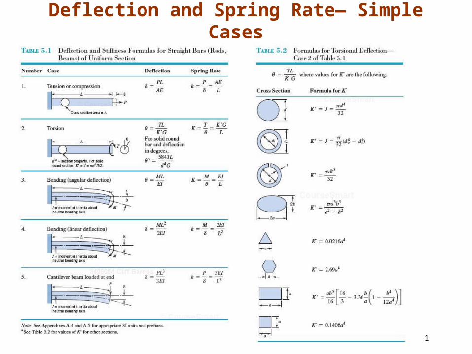
Deflection and Spring Rate— Simple Cases

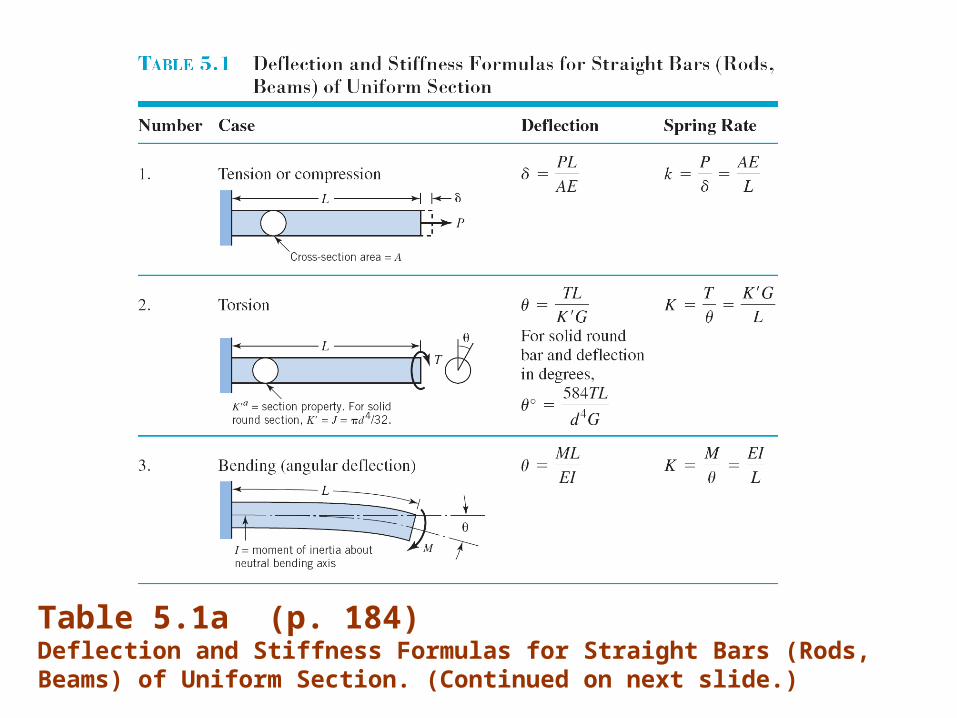
Table 5.1a (p. 184)Deflection and Stiffness Formulas for Straight Bars (Rods, Beams) of Uniform Section. (Continued on next slide.)

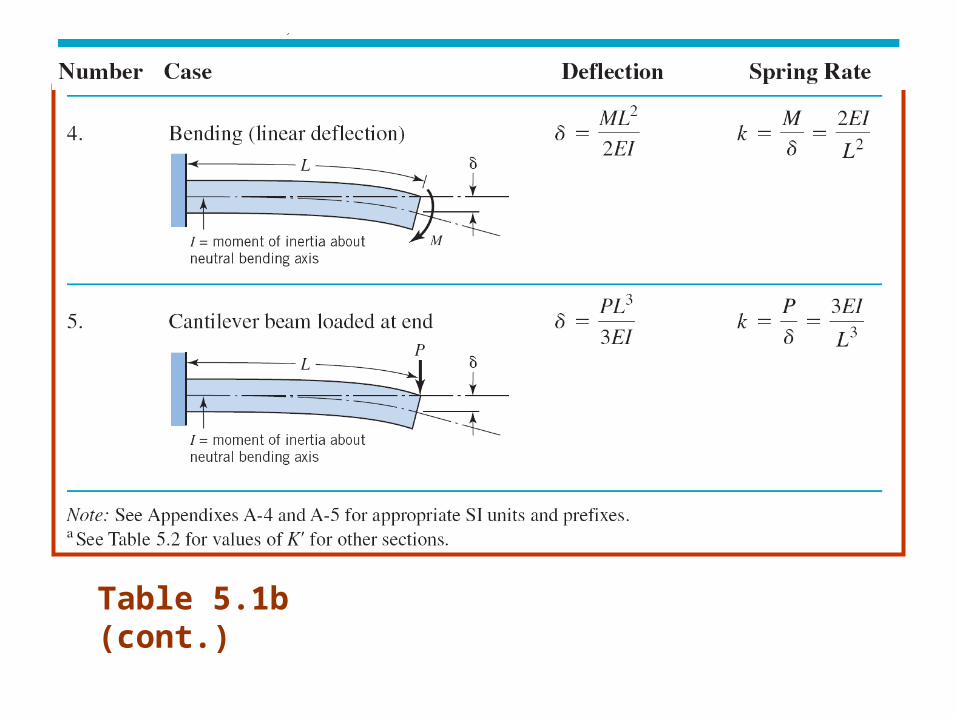
Table 5.1b (cont.)

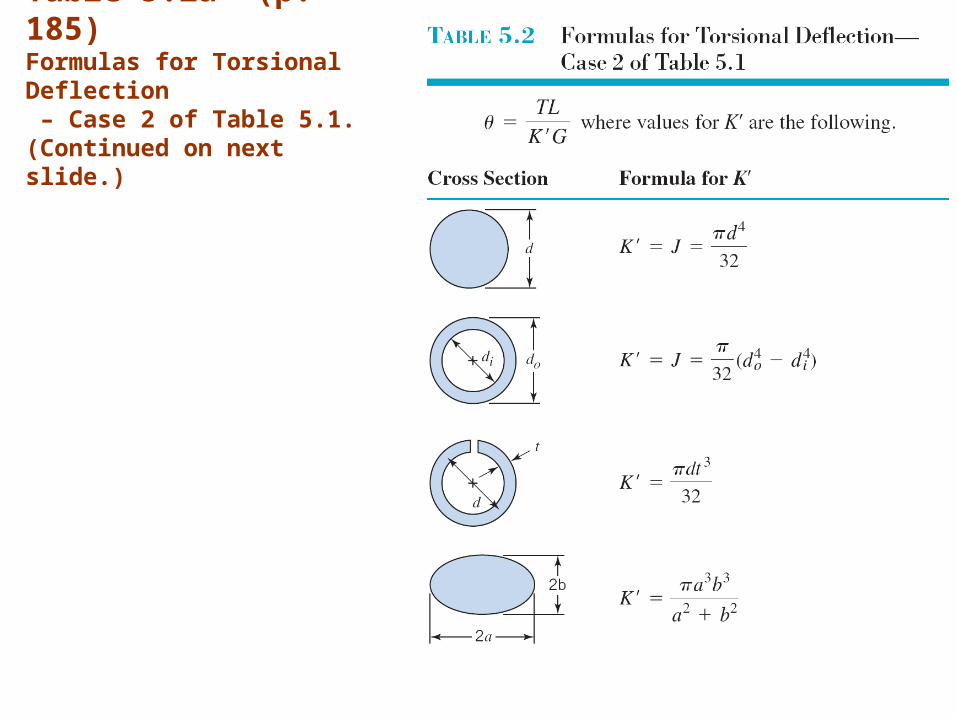
Table 5.2a (p. 185)Formulas for Torsional Deflection – Case 2 of Table 5.1.(Continued on next slide.)

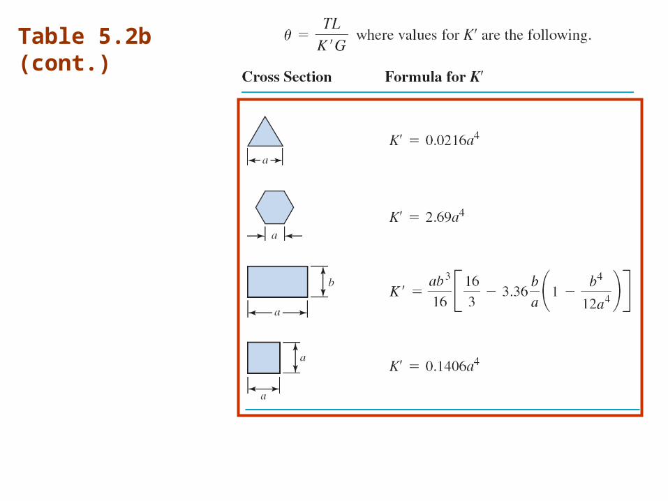
Table 5.2b (cont.)

6

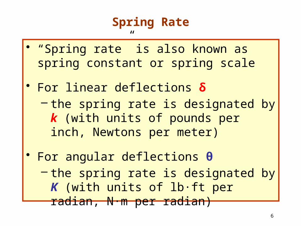
• “Spring rate” is also known as spring constant or spring scale

• For linear deflections δ – the spring rate is designated by k (with

units of pounds per inch, Newtons per meter)

• For angular deflections θ– the spring rate is designated by K (with

units of lb∙ft per radian, N∙m per radian)

Spring Rate

7

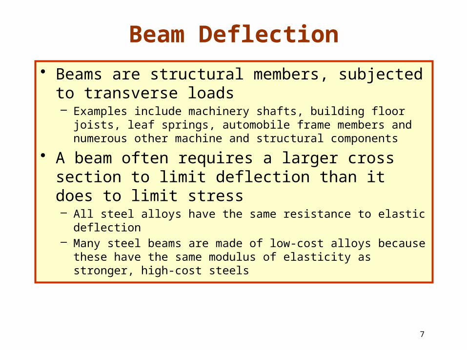
Beam Deflection• Beams are structural members, subjected to

transverse loads – Examples include machinery shafts, building floor joists, leaf

springs, automobile frame members and numerous other machine and structural components

• A beam often requires a larger cross section to limit deflection than it does to limit stress – All steel alloys have the same resistance to elastic deflection– Many steel beams are made of low-cost alloys because

these have the same modulus of elasticity as stronger, high-cost steels

8

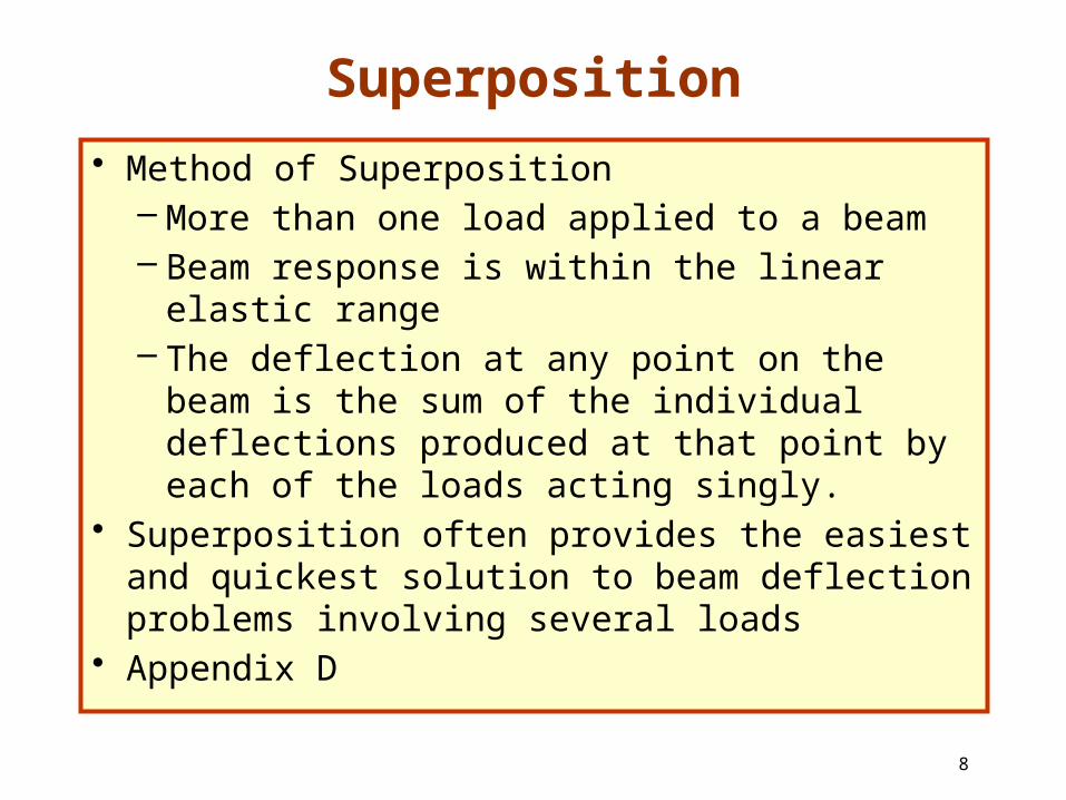
Superposition• Method of Superposition

– More than one load applied to a beam – Beam response is within the linear elastic

range – The deflection at any point on the beam is the

sum of the individual deflections produced at that point by each of the loads acting singly.

• Superposition often provides the easiest and quickest solution to beam deflection problems involving several loads

• Appendix D

9

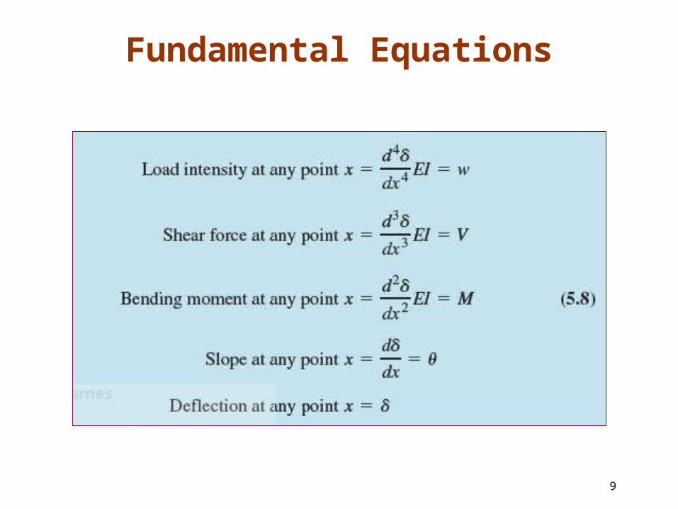
Fundamental Equations

10

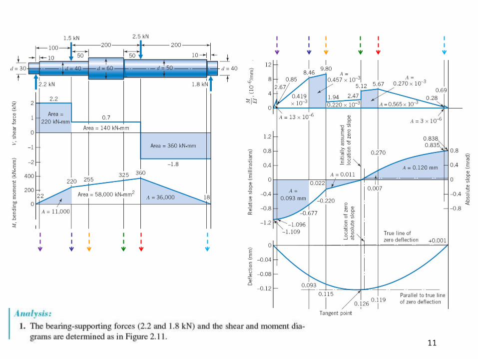
11

12

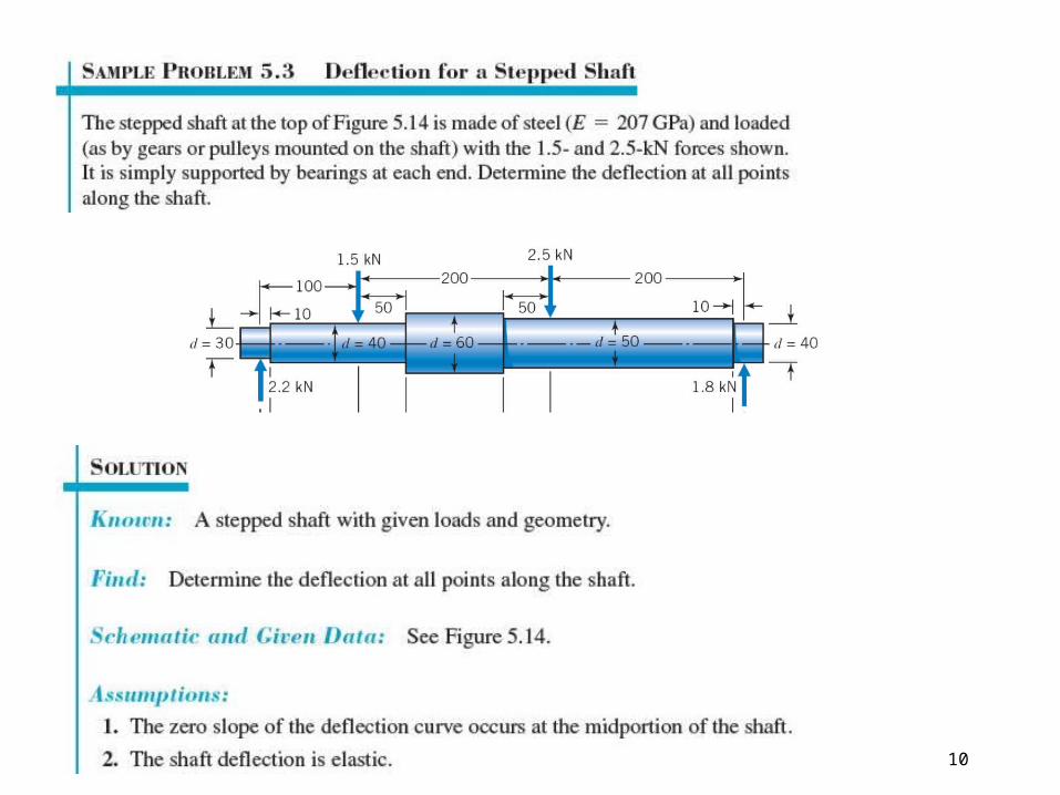
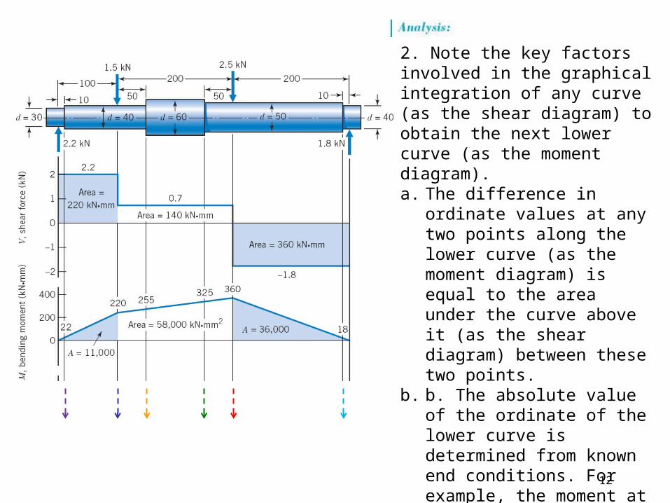
2. Note the key factors involved in the graphical integration of any curve (as the shear diagram) to obtain the next lower curve (as the moment diagram). a. The difference in ordinate values

at any two points along the lower curve (as the moment diagram) is equal to the area under the curve above it (as the shear diagram) between these two points.

b. b. The absolute value of the ordinate of the lower curve is determined from known end conditions. For example, the moment at the bearing supports is known to be zero.

c. c. The slope at any point on the lower curve is equal to the ordinate of the curve above.

13

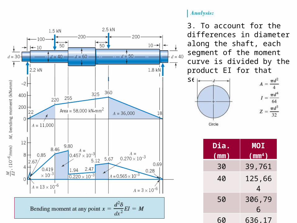
3. To account for the differences in diameter along the shaft, each segment of the moment curve is divided by the product EI for that segment.

E = 207 GPa

Values of IDia.

(mm)MOI

(mm4)30 39,761

40 125,664

50 306,796

60 636,173

14

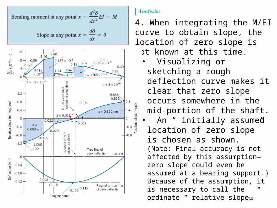
4. When integrating the M/EI curve to obtain slope, the location of zero slope is not known at this time.

• Visualizing or sketching a rough deflection curve makes it clear that zero slope occurs somewhere in the mid-portion of the shaft.

• An “ initially assumed location of zero slope” is chosen as shown. (Note: Final accuracy is not affected by this assumption— zero slope could even be assumed at a bearing support.) Because of the assumption, it is necessary to call the ordinate “ relative slope.”

15

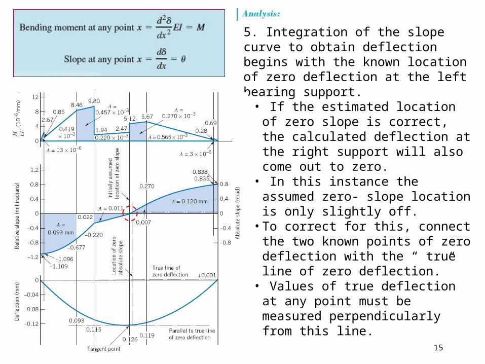
5. Integration of the slope curve to obtain deflection begins with the known location of zero deflection at the left bearing support.

• If the estimated location of zero slope is correct, the calculated deflection at the right support will also come out to zero.

• In this instance the assumed zero- slope location is only slightly off.

• To correct for this, connect the two known points of zero deflection with the “ true line of zero deflection.”

• Values of true deflection at any point must be measured perpendicularly from this line.

16

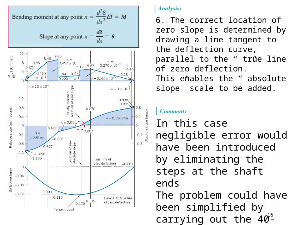
6. The correct location of zero slope is determined by drawing a line tangent to the deflection curve, parallel to the “ true line of zero deflection.” This enables the “ absolute slope” scale to be added.

In this case negligible error would have been introduced by eliminating the steps at the shaft endsThe problem could have been simplified by carrying out the 40- and 50- mm diameters to the ends.

17

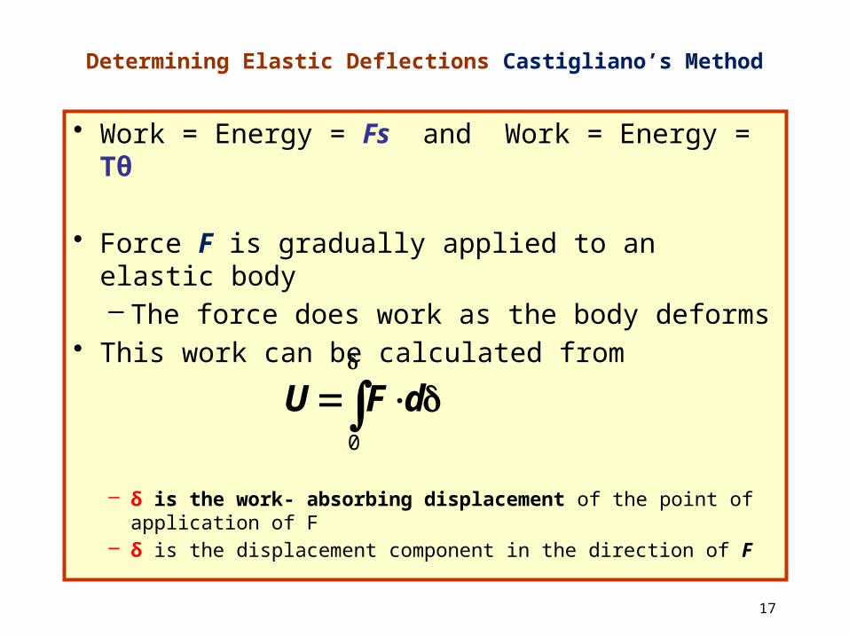
Determining Elastic Deflections Castigliano’s Method

• Work = Energy = Fs and Work = Energy = Tθ

• Force F is gradually applied to an elastic body – The force does work as the body deforms

• This work can be calculated from

– δ is the work- absorbing displacement of the point of application of F

– δ is the displacement component in the direction of F

0

dFU

18

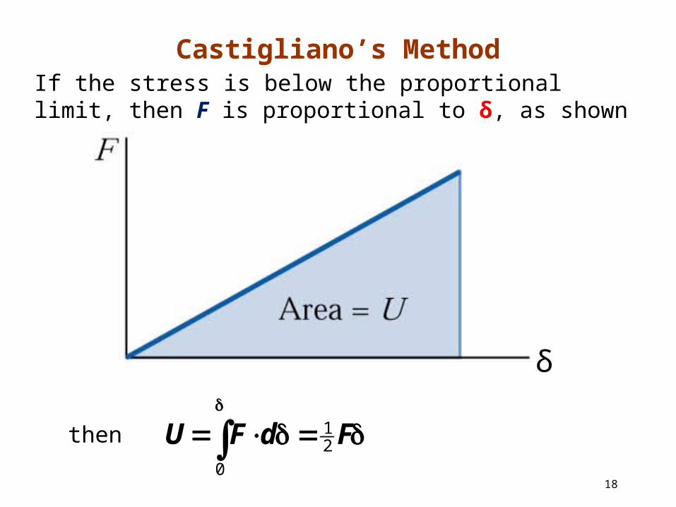
Castigliano’s MethodIf the stress is below the proportional limit, then F is proportional to δ, as shown

then

δ

FdFU 21

0

19

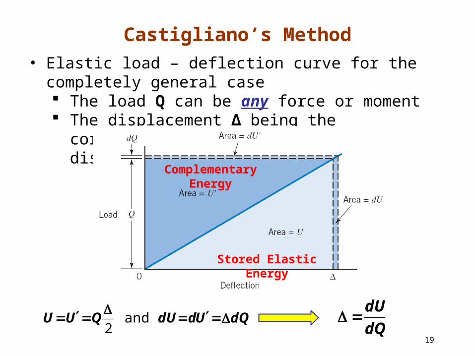
Castigliano’s Method• Elastic load – deflection curve for the completely general case

The load Q can be any force or moment The displacement Δ being the corresponding linear or

angular displacement

Stored Elastic Energy

Complementary Energy

dQUddUQUU

and 2

dQdU

20

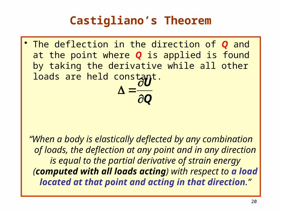
Castigliano’s Theorem

• The deflection in the direction of Q and at the point where Q is applied is found by taking the derivative while all other loads are held constant.

“When a body is elastically deflected by any combination of loads, the deflection at any point and in any direction

is equal to the partial derivative of strain energy (computed with all loads acting) with respect to a load

located at that point and acting in that direction.”

QU

21

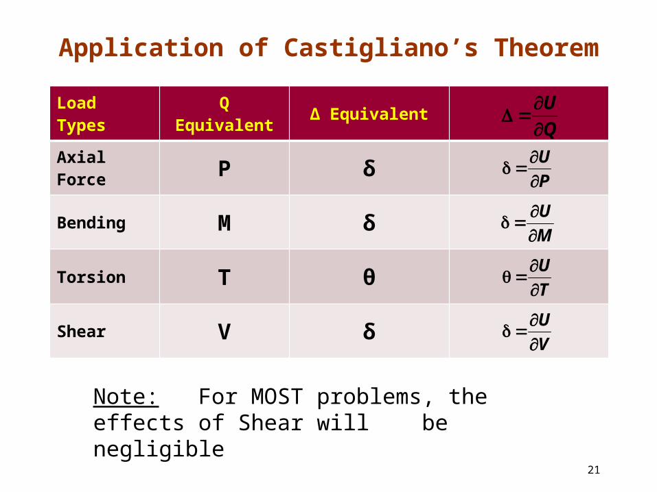
Load Types Q Equivalent Δ Equivalent

Axial Force P δBending M δTorsion T θShear V δ

PU

MU

TU

VU

Application of Castigliano’s Theorem

Note: For MOST problems, the effects of Shear will be negligible

QU

22

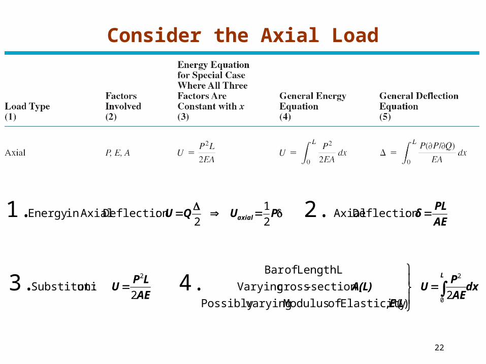
Consider the Axial Load

:Deflection Axial :Deflection AxialinEnergy 2.1.AEPLδPUQU axial

21

2

,Elasticity of Modulus varyingPossibly

section,-cross VaryingL Length of Bar

:onSubstituti 4.3. dxAEP

ULE

A(L)AE

LPU

L

0

22

2)(

2

23

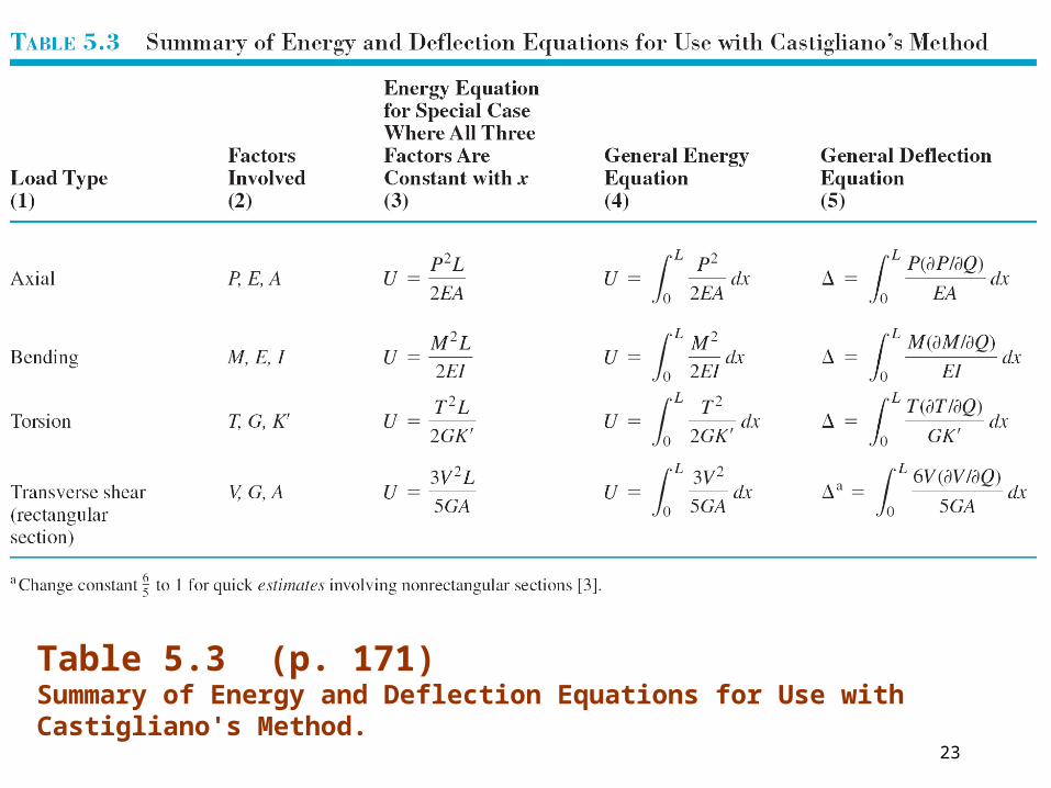
Table 5.3 (p. 171)Summary of Energy and Deflection Equations for Use with Castigliano's Method.

24

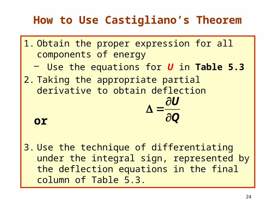
How to Use Castigliano’s Theorem

1. Obtain the proper expression for all components of energy– Use the equations for U in Table 5.3

2. Taking the appropriate partial derivative to obtain deflection

or

3. Use the technique of differentiating under the integral sign, represented by the deflection equations in the final column of Table 5.3.

QU

25

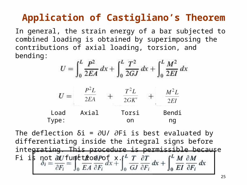
Application of Castigliano’s TheoremIn general, the strain energy of a bar subjected to combined loading is obtained by superimposing the contributions of axial loading, torsion, and bending:

The deflection δi = U/ Fi is best evaluated by differentiating inside the 𝜕 𝜕integral signs before integrating. This procedure is permissible because Fi is not a function of x.

AxialLoad Type: Torsion Bending

26

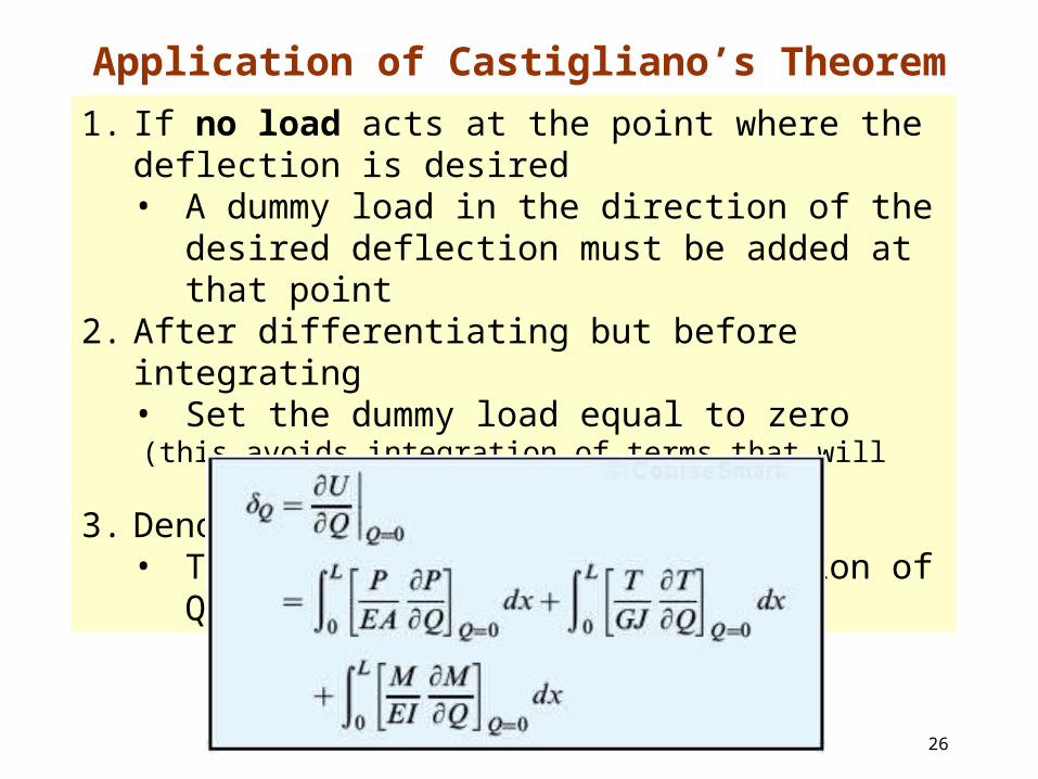
Application of Castigliano’s Theorem1. If no load acts at the point where the deflection is desired

• A dummy load in the direction of the desired deflection must be added at that point

2. After differentiating but before integrating • Set the dummy load equal to zero

(this avoids integration of terms that will eventually be set equal to zero) 3. Denote the dummy load by Q

• The displacement in the direction of Q thus is

27

Announcements (5th ed.)

HW05: 5.9, 5.13, 5.14, 5.15, 5.21, 5.26