Embed Size (px)
Citation preview
1© 2003 Thomson© 2003 Thomson/South-Western/South-Western Slide
Slides Prepared bySlides Prepared by
JOHN S. LOUCKSJOHN S. LOUCKSSt. Edward’s UniversitySt. Edward’s University
2© 2003 Thomson© 2003 Thomson/South-Western/South-Western Slide
Chapter 7Chapter 7Transportation, Assignment, and Transportation, Assignment, and
Transshipment ProblemsTransshipment Problems Transportation ProblemTransportation Problem
•Network Representation and LP FormulationNetwork Representation and LP Formulation•Transportation Simplex MethodTransportation Simplex Method
Assignment ProblemAssignment Problem•Network Representation and LP FormulationNetwork Representation and LP Formulation•Hungarian MethodHungarian Method
The Transshipment ProblemThe Transshipment Problem•Network Representation and LP FormulationNetwork Representation and LP Formulation
3© 2003 Thomson© 2003 Thomson/South-Western/South-Western Slide
Transportation, Assignment, and Transportation, Assignment, and Transshipment ProblemsTransshipment Problems
A A network modelnetwork model is one which can be is one which can be represented by a set of nodes, a set of arcs, represented by a set of nodes, a set of arcs, and functions (e.g. costs, supplies, demands, and functions (e.g. costs, supplies, demands, etc.) associated with the arcs and/or nodes.etc.) associated with the arcs and/or nodes.
Transportation, assignment, and Transportation, assignment, and transshipment problems of this chapter, as transshipment problems of this chapter, as well as the shortest route, minimal spanning well as the shortest route, minimal spanning tree, and maximal flow problems (Chapter 9) tree, and maximal flow problems (Chapter 9) and PERT/CPM problems (Chapter 10) are all and PERT/CPM problems (Chapter 10) are all examples of network problems.examples of network problems.
4© 2003 Thomson© 2003 Thomson/South-Western/South-Western Slide
Transportation, Assignment, and Transportation, Assignment, and Transshipment ProblemsTransshipment Problems
Each of the three models of this chapter Each of the three models of this chapter (transportation, assignment, and transshipment (transportation, assignment, and transshipment models) can be formulated as linear programs models) can be formulated as linear programs and solved by general purpose linear and solved by general purpose linear programming codes. programming codes.
For each of the three models, if the right-hand For each of the three models, if the right-hand side of the linear programming formulations are side of the linear programming formulations are all integers, the optimal solution will be in terms all integers, the optimal solution will be in terms of integer values for the decision variables.of integer values for the decision variables.
However, there are many computer packages However, there are many computer packages (including (including The Management ScientistThe Management Scientist) which ) which contain separate computer codes for these contain separate computer codes for these models which take advantage of their network models which take advantage of their network structure.structure.
5© 2003 Thomson© 2003 Thomson/South-Western/South-Western Slide
Transportation ProblemTransportation Problem The The transportation problemtransportation problem seeks to minimize seeks to minimize
the total shipping costs of transporting goods the total shipping costs of transporting goods from from mm origins (each with a supply origins (each with a supply ssii) to ) to nn destinations (each with a demand destinations (each with a demand ddjj), when ), when the unit shipping cost from an origin, the unit shipping cost from an origin, ii, to a , to a destination, destination, jj, is , is ccijij..
The The network representationnetwork representation for a for a transportation problem with two sources and transportation problem with two sources and three destinations is given on the next slide.three destinations is given on the next slide.
6© 2003 Thomson© 2003 Thomson/South-Western/South-Western Slide
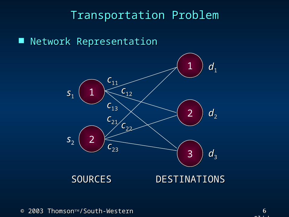
Transportation ProblemTransportation Problem Network RepresentationNetwork Representation
1
2
3
1
2
cc11
11 cc1212
cc1313cc2121 cc2222
cc2323
dd11
dd22
dd33
ss11
s2
SOURCESSOURCES DESTINATIONSDESTINATIONS
7© 2003 Thomson© 2003 Thomson/South-Western/South-Western Slide
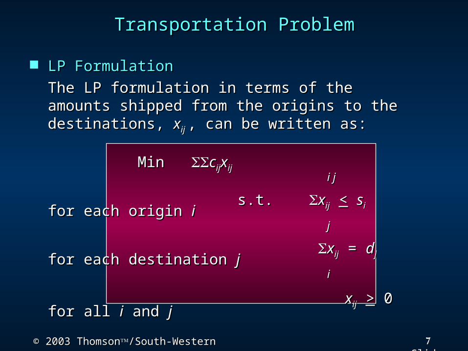
Transportation ProblemTransportation Problem LP FormulationLP Formulation
The LP formulation in terms of the The LP formulation in terms of the amounts shipped from the origins to the amounts shipped from the origins to the destinations, destinations, xxij ij , can be written as:, can be written as:
Min Min ccijijxxijij i ji j
s.t. s.t. xxijij << ssii for each origin for each origin ii jj xxijij = = ddjj for each for each destination destination jj ii xxijij >> 0 0 for all for all ii and and jj
8© 2003 Thomson© 2003 Thomson/South-Western/South-Western Slide
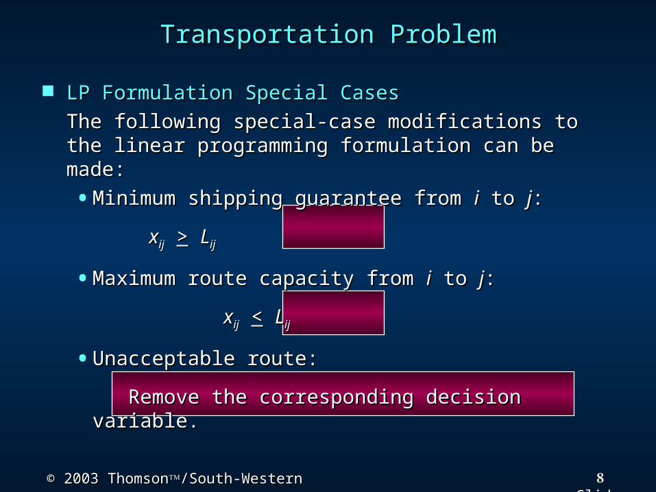
Transportation ProblemTransportation Problem LP Formulation Special CasesLP Formulation Special Cases
The following special-case modifications to the The following special-case modifications to the linear programming formulation can be made:linear programming formulation can be made:•Minimum shipping guarantee from Minimum shipping guarantee from ii to to jj: :
xxijij >> LLijij
•Maximum route capacity from Maximum route capacity from ii to to jj:: xxijij << LLijij
•Unacceptable route: Unacceptable route: Remove the corresponding decision variable.Remove the corresponding decision variable.
9© 2003 Thomson© 2003 Thomson/South-Western/South-Western Slide
Example: BBCExample: BBC
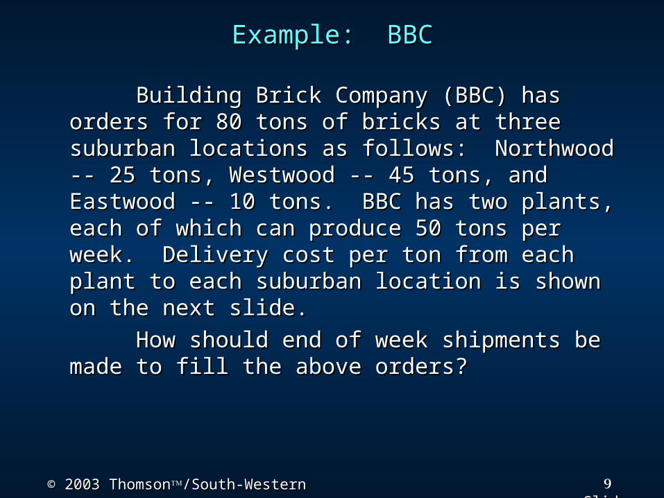
Building Brick Company (BBC) has orders Building Brick Company (BBC) has orders for 80 tons of bricks at three suburban locations for 80 tons of bricks at three suburban locations as follows: Northwood -- 25 tons, Westwood -- as follows: Northwood -- 25 tons, Westwood -- 45 tons, and Eastwood -- 10 tons. BBC has two 45 tons, and Eastwood -- 10 tons. BBC has two plants, each of which can produce 50 tons per plants, each of which can produce 50 tons per week. Delivery cost per ton from each plant to week. Delivery cost per ton from each plant to each suburban location is shown on the next each suburban location is shown on the next slide.slide.
How should end of week shipments be How should end of week shipments be made to fill the above orders?made to fill the above orders?
10© 2003 Thomson© 2003 Thomson/South-Western/South-Western Slide
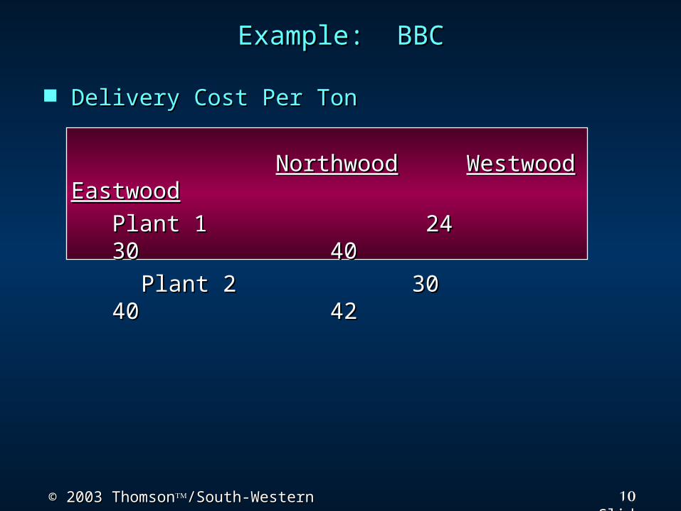
Example: BBCExample: BBC Delivery Cost Per TonDelivery Cost Per Ton
NorthwoodNorthwood WestwoodWestwood EastwoodEastwood Plant 1 24 Plant 1 24 30 30 40 40
Plant 2 Plant 2 30 40 30 40 42 42
11© 2003 Thomson© 2003 Thomson/South-Western/South-Western Slide
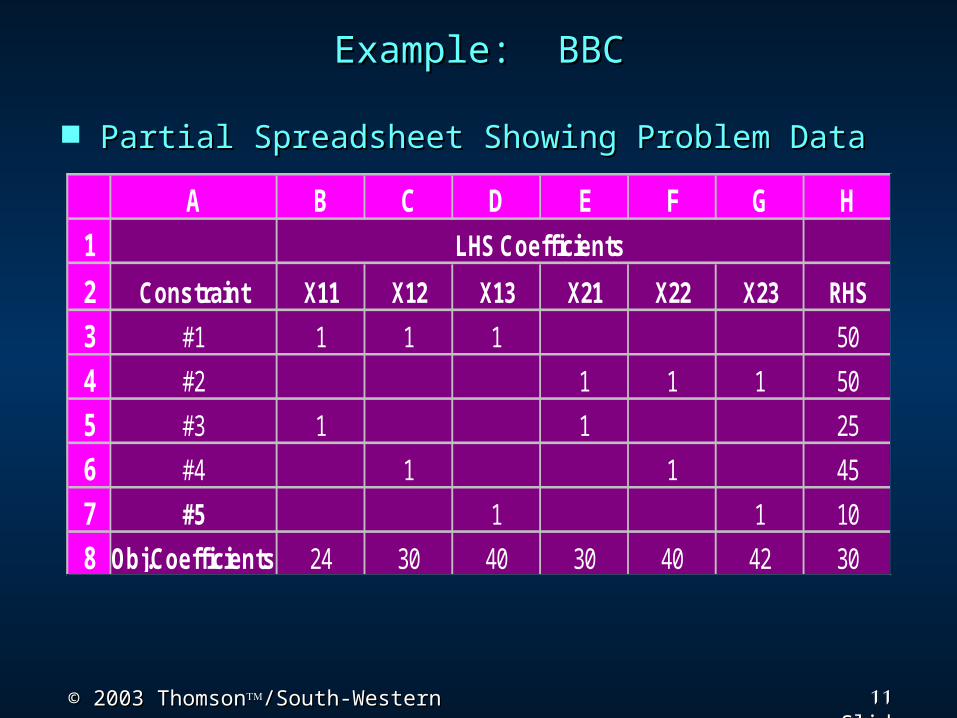
Example: BBCExample: BBC Partial Spreadsheet Showing Problem DataPartial Spreadsheet Showing Problem Data
A B C D E F G H12 Constraint X11 X12 X13 X21 X22 X23 RHS3 #1 1 1 1 504 #2 1 1 1 505 #3 1 1 256 #4 1 1 457 #5 1 1 108 Obj.Coefficients 24 30 40 30 40 42 30
LHS Coefficients
12© 2003 Thomson© 2003 Thomson/South-Western/South-Western Slide
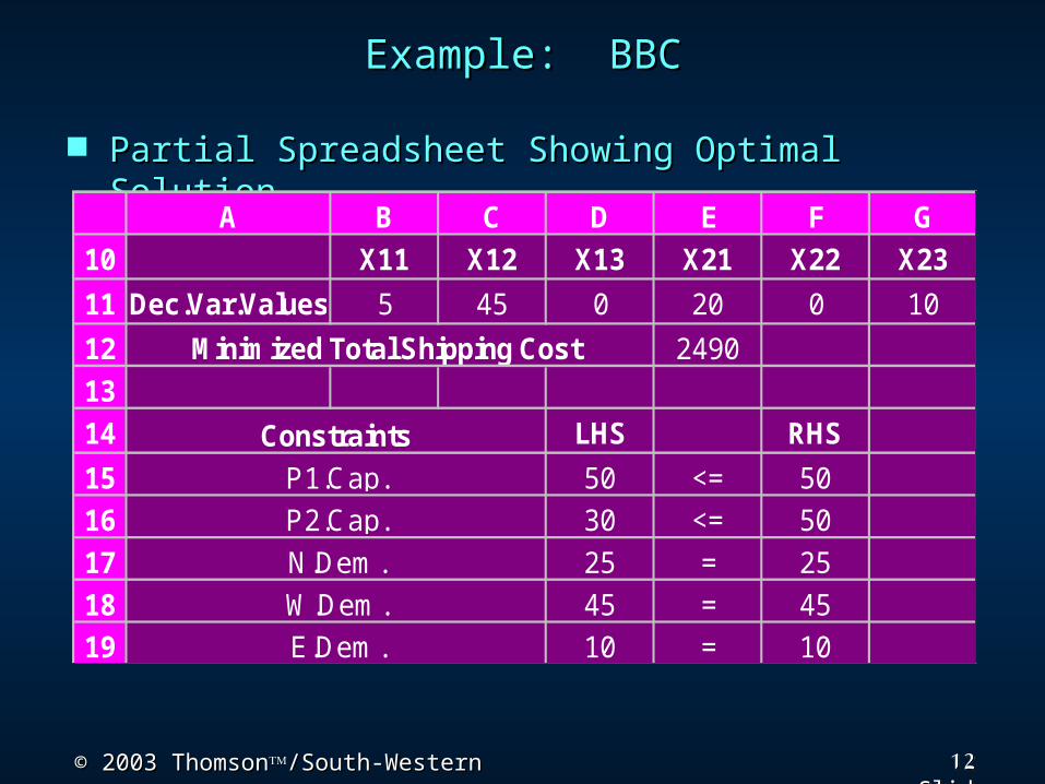
Example: BBCExample: BBC Partial Spreadsheet Showing Optimal SolutionPartial Spreadsheet Showing Optimal Solution
A B C D E F G10 X11 X12 X13 X21 X22 X2311 Dec.Var.Values 5 45 0 20 0 1012 Minimized Total Shipping Cost 24901314 LHS RHS15 50 <= 5016 30 <= 5017 25 = 2518 45 = 4519 10 = 10E.Dem.
W.Dem.N.Dem.
ConstraintsP1.Cap.P2.Cap.
13© 2003 Thomson© 2003 Thomson/South-Western/South-Western Slide
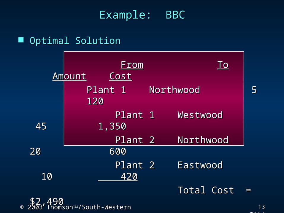
Optimal SolutionOptimal Solution
FromFrom ToTo AmountAmount CostCost
Plant 1 Northwood 5 Plant 1 Northwood 5 120120
Plant 1 Westwood 45 Plant 1 Westwood 45 1,3501,350
Plant 2 Northwood 20 Plant 2 Northwood 20 600600
Plant 2 Eastwood 10 Plant 2 Eastwood 10 420420
Total Cost = $2,490Total Cost = $2,490
Example: BBCExample: BBC
14© 2003 Thomson© 2003 Thomson/South-Western/South-Western Slide
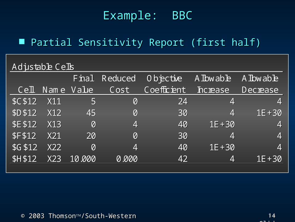
Example: BBCExample: BBC Partial Sensitivity Report (first half)Partial Sensitivity Report (first half)
Adjustable CellsFinal Reduced Objective Allowable Allowable
Cell Name Value Cost Coefficient Increase Decrease$C$12 X11 5 0 24 4 4$D$12 X12 45 0 30 4 1E+30$E$12 X13 0 4 40 1E+30 4$F$12 X21 20 0 30 4 4$G$12 X22 0 4 40 1E+30 4$H$12 X23 10.000 0.000 42 4 1E+30
15© 2003 Thomson© 2003 Thomson/South-Western/South-Western Slide
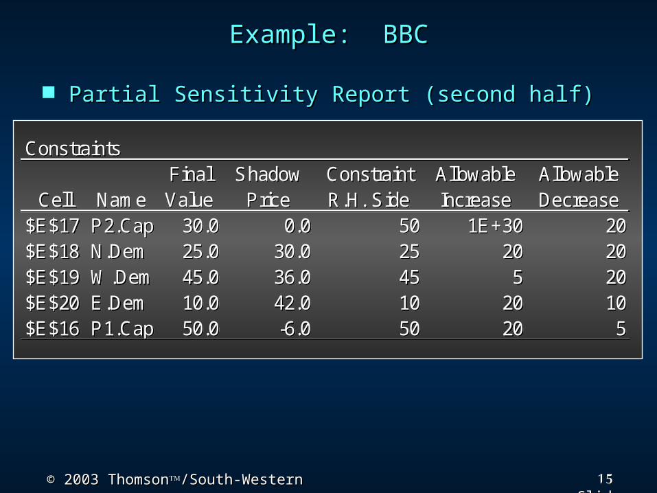
Example: BBCExample: BBC Partial Sensitivity Report (second half)Partial Sensitivity Report (second half)
ConstraintsFinal Shadow Constraint Allowable Allowable
Cell Name Value Price R.H. Side Increase Decrease$E$17 P2.Cap 30.0 0.0 50 1E+30 20$E$18 N.Dem 25.0 30.0 25 20 20$E$19 W.Dem 45.0 36.0 45 5 20$E$20 E.Dem 10.0 42.0 10 20 10$E$16 P1.Cap 50.0 -6.0 50 20 5
16© 2003 Thomson© 2003 Thomson/South-Western/South-Western Slide
Transportation Simplex MethodTransportation Simplex Method The transportation simplex method requires that The transportation simplex method requires that
the sum of the supplies at the origins equal the the sum of the supplies at the origins equal the sum of the demands at the destinations. sum of the demands at the destinations.
If the total supply is greater than the total If the total supply is greater than the total demand, a dummy destination is added with demand, a dummy destination is added with demand equal to the excess supply, and shipping demand equal to the excess supply, and shipping costs from all origins are zero. (If total supply is costs from all origins are zero. (If total supply is less than total demand, a dummy origin is added.)less than total demand, a dummy origin is added.)
When solving a transportation problem by its When solving a transportation problem by its special purpose algorithm, unacceptable shipping special purpose algorithm, unacceptable shipping routes are given a cost of +routes are given a cost of +MM (a large number). (a large number).
17© 2003 Thomson© 2003 Thomson/South-Western/South-Western Slide
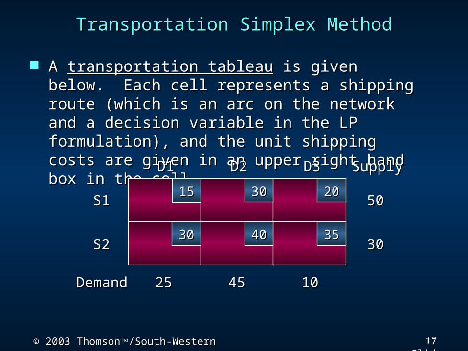
Transportation Simplex MethodTransportation Simplex Method A A transportation tableautransportation tableau is given below. Each is given below. Each
cell represents a shipping route (which is an cell represents a shipping route (which is an arc on the network and a decision variable in arc on the network and a decision variable in the LP formulation), and the unit shipping the LP formulation), and the unit shipping costs are given in an upper right hand box in costs are given in an upper right hand box in the cell. the cell. SupplySupply
3030
5050
3535
2020
4040
3030
3030
DemandDemand 101045452525
S1S1
S2S2
D3D3D2D2D1D11515
18© 2003 Thomson© 2003 Thomson/South-Western/South-Western Slide
Transportation Simplex MethodTransportation Simplex Method The transportation problem is solved in The transportation problem is solved in two two
phasesphases: : •Phase I -- Obtaining an initial feasible solutionPhase I -- Obtaining an initial feasible solution•Phase II -- Moving toward optimalityPhase II -- Moving toward optimality
Phase I:Phase I: The Minimum-Cost Procedure can be The Minimum-Cost Procedure can be used to establish an initial basic feasible solution used to establish an initial basic feasible solution without doing numerous iterations of the simplex without doing numerous iterations of the simplex method.method.
Phase II:Phase II: The Stepping Stone Method - using the The Stepping Stone Method - using the MODI Method for evaluating the reduced costs - MODI Method for evaluating the reduced costs - may be used to move from the initial feasible may be used to move from the initial feasible solution to the optimal one.solution to the optimal one.
19© 2003 Thomson© 2003 Thomson/South-Western/South-Western Slide
Transportation Simplex MethodTransportation Simplex Method Phase I - Minimum-Cost MethodPhase I - Minimum-Cost Method
•Step 1:Step 1: Select the cell with the least cost. Select the cell with the least cost. Assign to this cell the minimum of its Assign to this cell the minimum of its remaining row supply or remaining column remaining row supply or remaining column demand.demand.
•Step 2:Step 2: Decrease the row and column Decrease the row and column availabilities by this amount and remove from availabilities by this amount and remove from consideration all other cells in the row or consideration all other cells in the row or column with zero availability/demand. (If both column with zero availability/demand. (If both are simultaneously reduced to 0, assign an are simultaneously reduced to 0, assign an allocation of 0 to any other unoccupied cell in allocation of 0 to any other unoccupied cell in the row or column before deleting both.) GO the row or column before deleting both.) GO TO STEP 1.TO STEP 1.
20© 2003 Thomson© 2003 Thomson/South-Western/South-Western Slide
Transportation Simplex MethodTransportation Simplex Method Phase II - Stepping Stone MethodPhase II - Stepping Stone Method
•Step 1:Step 1: For each unoccupied cell, calculate the For each unoccupied cell, calculate the reduced cost by the MODI method described on reduced cost by the MODI method described on an upcoming slide. an upcoming slide.
Select the unoccupied cell with the Select the unoccupied cell with the most negative reduced cost. (For maximization most negative reduced cost. (For maximization problems select the unoccupied cell with the problems select the unoccupied cell with the largest reduced cost.) If none, STOP.largest reduced cost.) If none, STOP.
21© 2003 Thomson© 2003 Thomson/South-Western/South-Western Slide
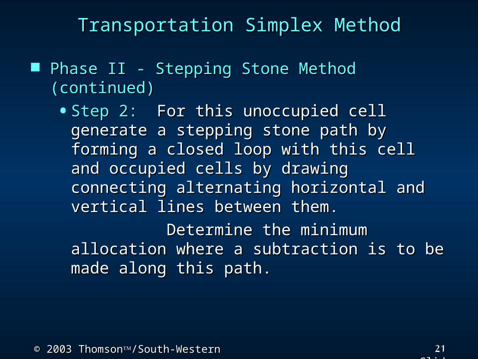
Transportation Simplex MethodTransportation Simplex Method Phase II - Stepping Stone Method (continued)Phase II - Stepping Stone Method (continued)
•Step 2:Step 2: For this unoccupied cell generate a For this unoccupied cell generate a stepping stone path by forming a closed loop stepping stone path by forming a closed loop with this cell and occupied cells by drawing with this cell and occupied cells by drawing connecting alternating horizontal and vertical connecting alternating horizontal and vertical lines between them. lines between them.
Determine the minimum allocation Determine the minimum allocation where a subtraction is to be made along this where a subtraction is to be made along this path. path.
22© 2003 Thomson© 2003 Thomson/South-Western/South-Western Slide
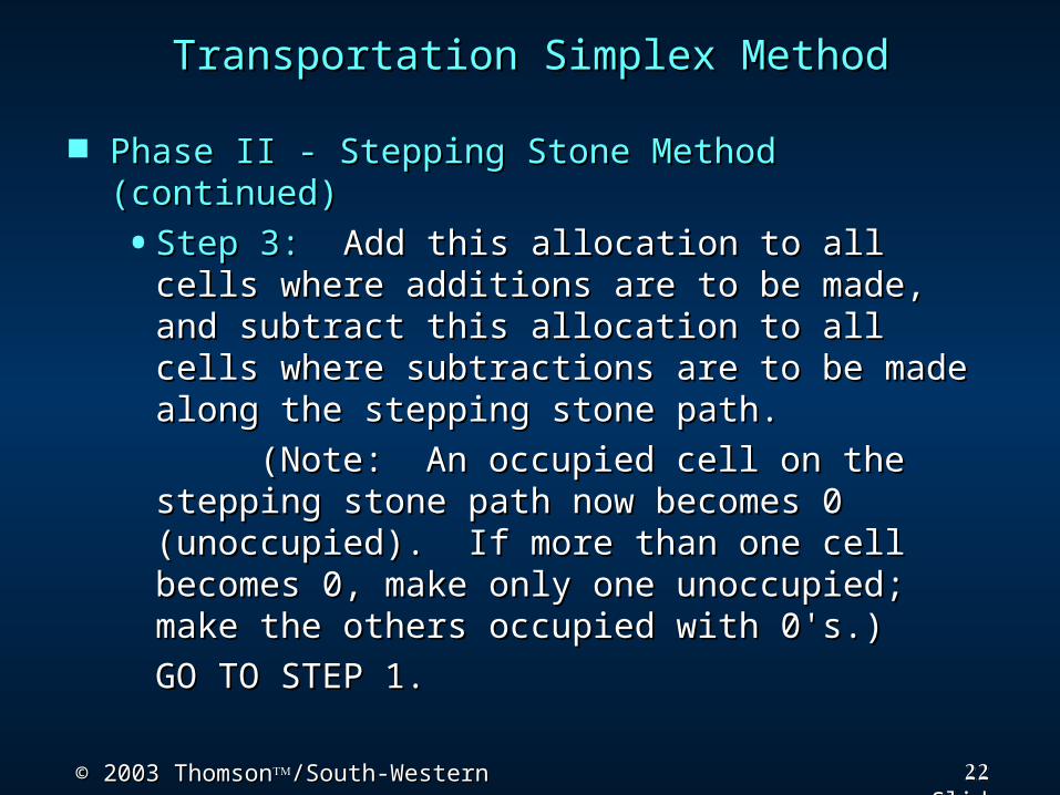
Transportation Simplex MethodTransportation Simplex Method Phase II - Stepping Stone Method (continued)Phase II - Stepping Stone Method (continued)
•Step 3:Step 3: Add this allocation to all cells where Add this allocation to all cells where additions are to be made, and subtract this additions are to be made, and subtract this allocation to all cells where subtractions are to allocation to all cells where subtractions are to be made along the stepping stone path. be made along the stepping stone path. (Note: An occupied cell on the (Note: An occupied cell on the stepping stone path now becomes 0 stepping stone path now becomes 0 (unoccupied). If more than one cell becomes (unoccupied). If more than one cell becomes 0, make only one unoccupied; make the 0, make only one unoccupied; make the others occupied with 0's.) others occupied with 0's.)
GO TO STEP 1.GO TO STEP 1.
23© 2003 Thomson© 2003 Thomson/South-Western/South-Western Slide
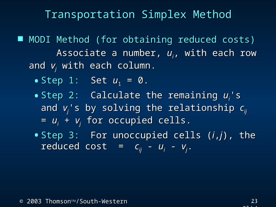
Transportation Simplex MethodTransportation Simplex Method MODI Method (for obtaining reduced costs)MODI Method (for obtaining reduced costs)
Associate a number, Associate a number, uuii, with each row and , with each row and vvjj with each column. with each column.•Step 1:Step 1: Set Set uu11 = 0. = 0.•Step 2:Step 2: Calculate the remaining Calculate the remaining uuii's and 's and vvjj's 's
by solving the relationship by solving the relationship ccijij = = uuii + + vvjj for for occupied cells.occupied cells.
•Step 3:Step 3: For unoccupied cells (For unoccupied cells (ii,,jj), the reduced ), the reduced cost = cost = ccijij - - uuii - - vvjj..
24© 2003 Thomson© 2003 Thomson/South-Western/South-Western Slide
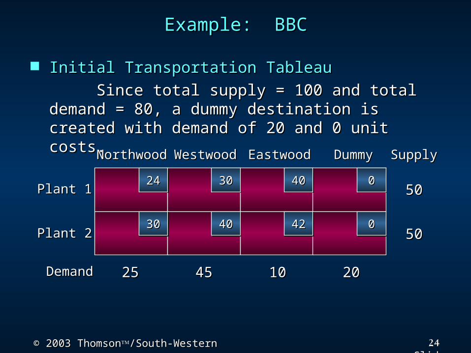
Example: BBCExample: BBC Initial Transportation TableauInitial Transportation Tableau
Since total supply = 100 and total demand Since total supply = 100 and total demand = 80, a dummy destination is created with = 80, a dummy destination is created with demand of 20 and 0 unit costs.demand of 20 and 0 unit costs.
4242
4040 00
004040
3030
3030
DemandDemand
SupplySupply
5050
5050
2020101045452525
DummyDummy
Plant 1Plant 1
Plant 2Plant 2
EastwoodEastwoodWestwoodWestwoodNorthwoodNorthwood2424
25© 2003 Thomson© 2003 Thomson/South-Western/South-Western Slide
Example: BBCExample: BBC Phase I: Minimum-Cost ProcedurePhase I: Minimum-Cost Procedure
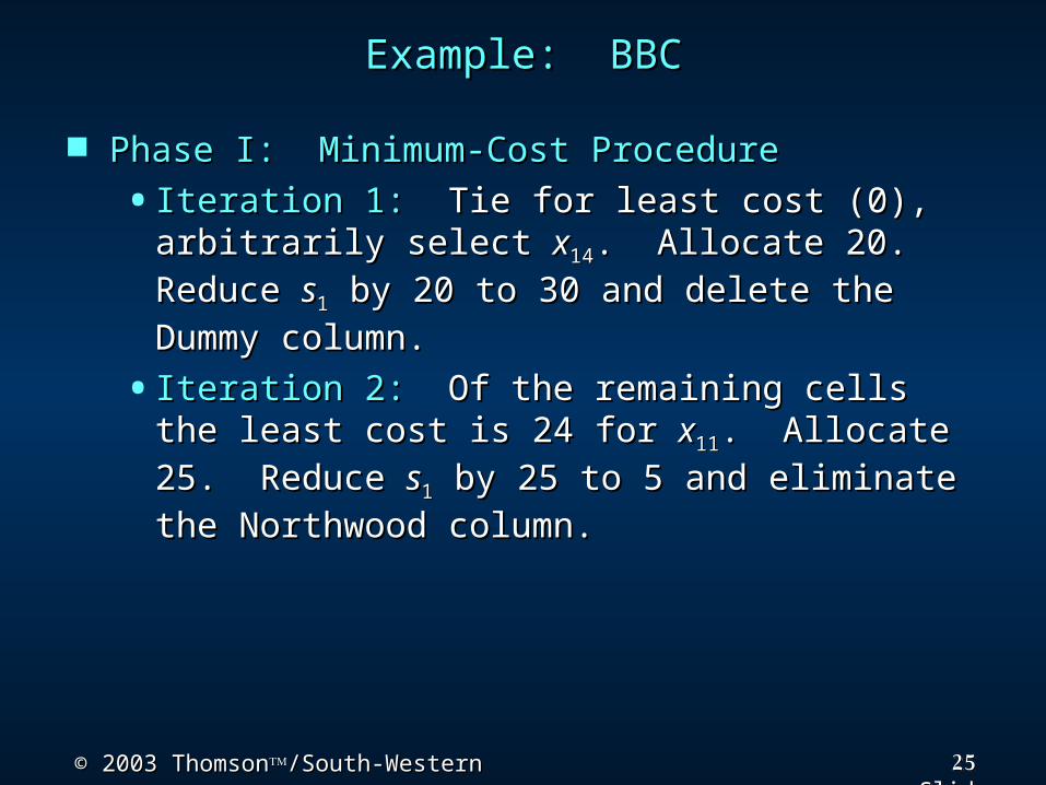
• Iteration 1:Iteration 1: Tie for least cost (0), arbitrarily Tie for least cost (0), arbitrarily select select xx1414. Allocate 20. Reduce . Allocate 20. Reduce ss11 by 20 to 30 by 20 to 30 and delete the Dummy column.and delete the Dummy column.
• Iteration 2:Iteration 2: Of the remaining cells the least Of the remaining cells the least cost is 24 for cost is 24 for xx1111. Allocate 25. Reduce . Allocate 25. Reduce ss11 by by 25 to 5 and eliminate the Northwood column.25 to 5 and eliminate the Northwood column.
26© 2003 Thomson© 2003 Thomson/South-Western/South-Western Slide
Example: BBCExample: BBC Phase I: Minimum-Cost Procedure (continued)Phase I: Minimum-Cost Procedure (continued)
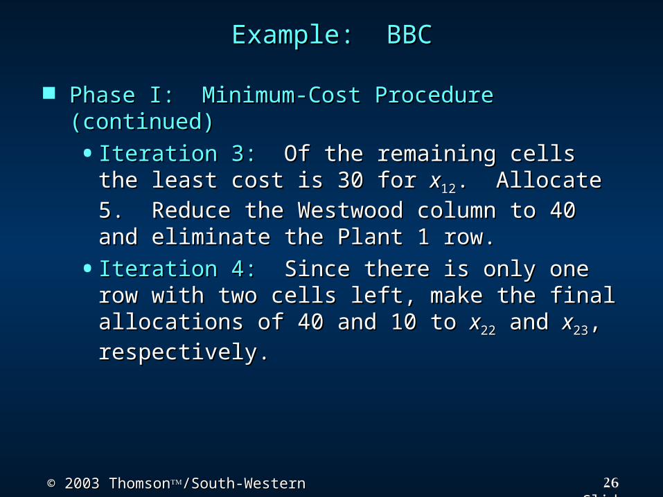
• Iteration 3:Iteration 3: Of the remaining cells the least Of the remaining cells the least cost is 30 for cost is 30 for xx1212. Allocate 5. Reduce the . Allocate 5. Reduce the Westwood column to 40 and eliminate the Westwood column to 40 and eliminate the Plant 1 row.Plant 1 row.
• Iteration 4:Iteration 4: Since there is only one row with Since there is only one row with two cells left, make the final allocations of 40 two cells left, make the final allocations of 40 and 10 to and 10 to xx2222 and and xx2323, respectively., respectively.
27© 2003 Thomson© 2003 Thomson/South-Western/South-Western Slide
Example: BBCExample: BBC Phase II – Iteration 1Phase II – Iteration 1
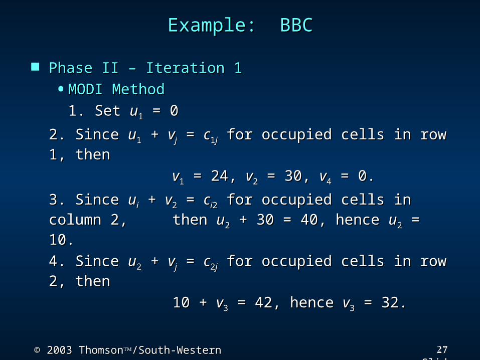
•MODI MethodMODI Method1. Set 1. Set uu11 = 0 = 0
2. Since 2. Since uu11 + + vvjj = = cc11jj for occupied cells in for occupied cells in row 1, thenrow 1, then
vv11 = 24, = 24, vv22 = 30, = 30, vv44 = 0. = 0.3. Since 3. Since uuii + + vv22 = = ccii22 for occupied cells in for occupied cells in
column 2, column 2, then then uu22 + 30 = 40, hence + 30 = 40, hence uu22 = 10. = 10.4. Since 4. Since uu22 + + vvjj = = cc22jj for occupied cells in for occupied cells in
row 2, thenrow 2, then 10 + 10 + vv33 = 42, hence = 42, hence vv33 = 32. = 32.
28© 2003 Thomson© 2003 Thomson/South-Western/South-Western Slide
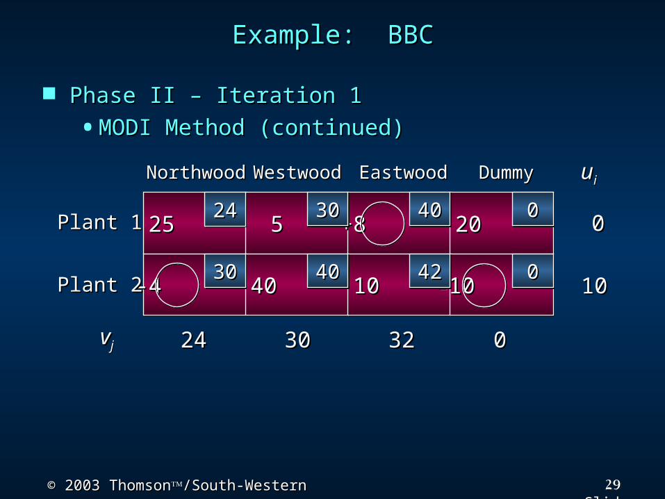
Example: BBCExample: BBC Phase II – Iteration 1Phase II – Iteration 1
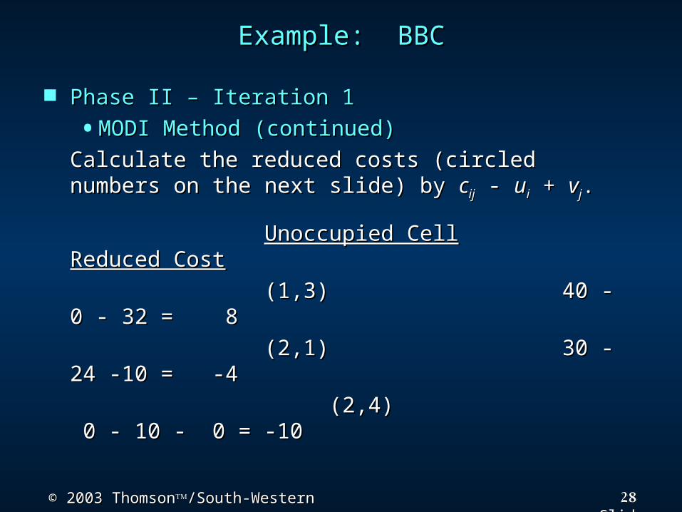
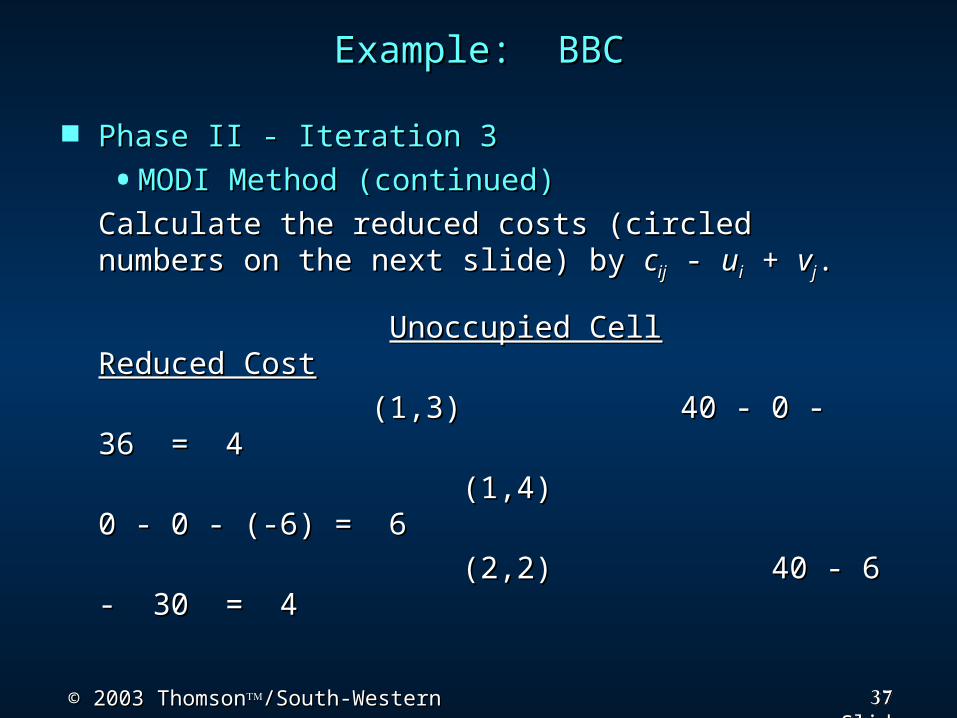
•MODI Method (continued)MODI Method (continued)Calculate the reduced costs (circled Calculate the reduced costs (circled
numbers on the numbers on the next slide) by next slide) by ccijij - - uuii + + vvjj..
Unoccupied CellUnoccupied Cell Reduced CostReduced Cost (1,3) 40 - 0 - 32 = (1,3) 40 - 0 - 32 =
88 (2,1) 30 - 24 -10 = (2,1) 30 - 24 -10 =
-4-4 (2,4) 0 - 10 - 0 = -(2,4) 0 - 10 - 0 = -
1010
29© 2003 Thomson© 2003 Thomson/South-Western/South-Western Slide
Example: BBCExample: BBC Phase II – Iteration 1Phase II – Iteration 1
•MODI Method (continued)MODI Method (continued)
2525 5 5
-4 -4
+8 +8 20 20
40 40 10 10 -10 -10 4242
4040 00
004040
3030
3030
vvjj
uuii
1010
00
00323230302424
DummyDummy
Plant 1Plant 1
Plant 2Plant 2
EastwoodEastwoodWestwoodWestwoodNorthwoodNorthwood
2424
30© 2003 Thomson© 2003 Thomson/South-Western/South-Western Slide
Example: BBCExample: BBC Phase II – Iteration 1Phase II – Iteration 1
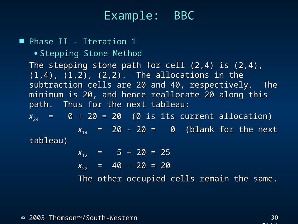
•Stepping Stone MethodStepping Stone MethodThe stepping stone path for cell (2,4) is (2,4), (1,4), The stepping stone path for cell (2,4) is (2,4), (1,4), (1,2), (2,2). The allocations in the subtraction cells (1,2), (2,2). The allocations in the subtraction cells are 20 and 40, respectively. The minimum is 20, and are 20 and 40, respectively. The minimum is 20, and hence reallocate 20 along this path. Thus for the next hence reallocate 20 along this path. Thus for the next tableau:tableau:xx2424 = 0 + 20 = 20 (0 is its current allocation) = 0 + 20 = 20 (0 is its current allocation)
xx1414 = 20 - 20 = 0 (blank for the next tableau) = 20 - 20 = 0 (blank for the next tableau) xx1212 = 5 + 20 = 25 = 5 + 20 = 25 xx2222 = 40 - 20 = 20 = 40 - 20 = 20 The other occupied cells remain the same.The other occupied cells remain the same.
31© 2003 Thomson© 2003 Thomson/South-Western/South-Western Slide
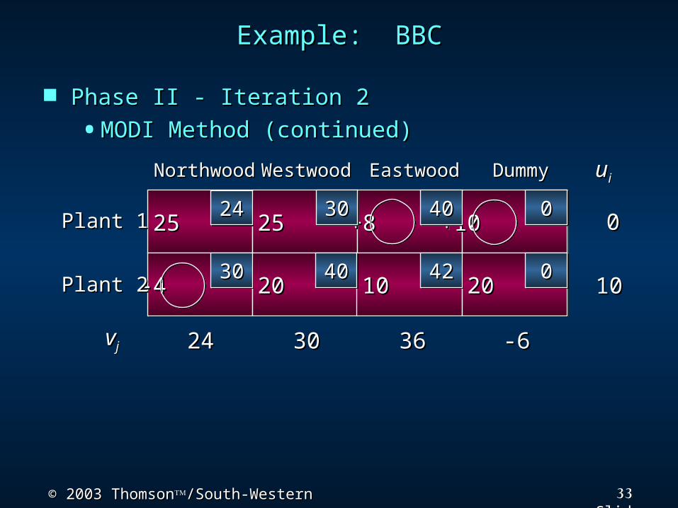
Example: BBCExample: BBC Phase II - Iteration 2Phase II - Iteration 2
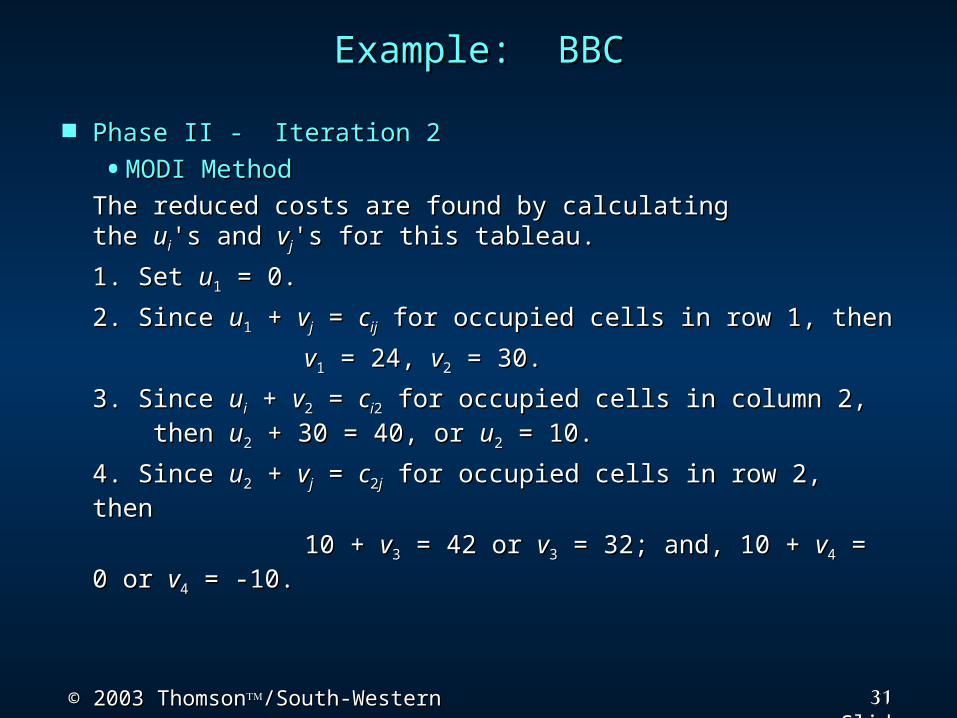
•MODI MethodMODI MethodThe reduced costs are found by calculating The reduced costs are found by calculating the the uuii's 's and and vvjj's for this tableau.'s for this tableau.1. Set 1. Set uu11 = 0. = 0.2. Since 2. Since uu11 + + vvjj = = ccijij for occupied cells in row 1, then for occupied cells in row 1, then
vv11 = 24, = 24, vv22 = 30. = 30.3. Since 3. Since uuii + + vv22 = = ccii22 for occupied cells in column 2, for occupied cells in column 2, then then uu22 + 30 = 40, or + 30 = 40, or uu22 = 10. = 10.4. Since 4. Since uu22 + + vvjj = = cc22jj for occupied cells in row 2, then for occupied cells in row 2, then
10 + 10 + vv33 = 42 or = 42 or vv33 = 32; and, 10 + = 32; and, 10 + vv44 = 0 or = 0 or vv44 = -10.= -10.
32© 2003 Thomson© 2003 Thomson/South-Western/South-Western Slide
Example: BBCExample: BBC Phase II - Iteration 2Phase II - Iteration 2
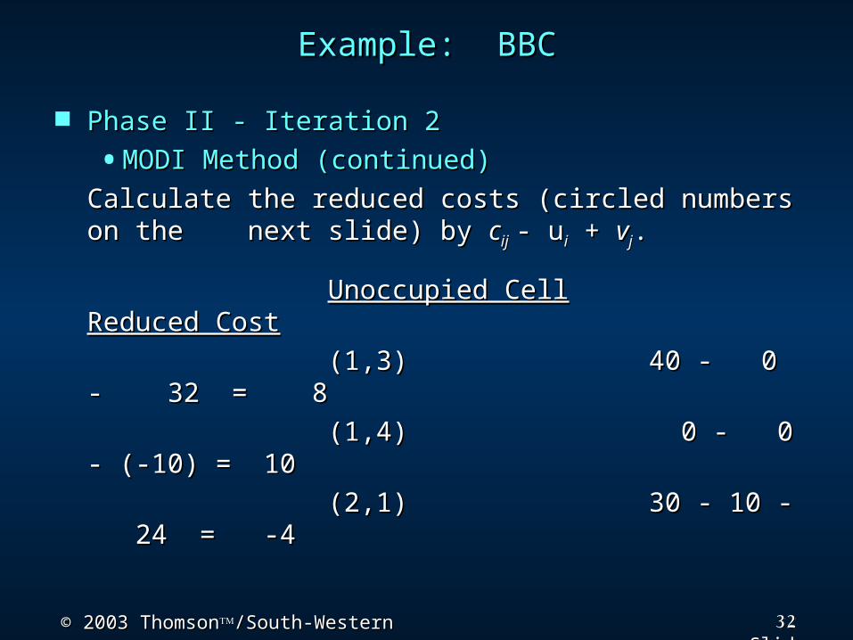
•MODI Method (continued)MODI Method (continued)Calculate the reduced costs (circled Calculate the reduced costs (circled
numbers on the numbers on the next slide) by next slide) by ccijij - u- uii + + vvjj..
Unoccupied CellUnoccupied Cell Reduced CostReduced Cost (1,3) (1,3) 40 - 0 - 32 = 40 - 0 - 32 =
88 (1,4) (1,4) 0 - 0 - (- 0 - 0 - (-
10) = 1010) = 10 (2,1) (2,1) 30 - 10 - 24 = -30 - 10 - 24 = -
44
33© 2003 Thomson© 2003 Thomson/South-Western/South-Western Slide
Example: BBCExample: BBC Phase II - Iteration 2Phase II - Iteration 2
•MODI Method (continued)MODI Method (continued)
2525 25 25
-4 -4
+8 +8 +10 +10
20 20 10 10 20 20 4242
4040 00
004040
3030
3030
vvjj
uuii
1010
00
-6-6363630302424
DummyDummy
Plant 1Plant 1
Plant 2Plant 2
EastwoodEastwoodWestwoodWestwoodNorthwoodNorthwood
2424
34© 2003 Thomson© 2003 Thomson/South-Western/South-Western Slide
Example: BBCExample: BBC Phase II - Iteration 2Phase II - Iteration 2
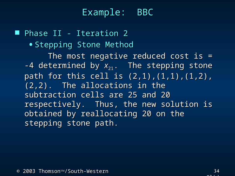
•Stepping Stone MethodStepping Stone MethodThe most negative reduced cost is = -4 The most negative reduced cost is = -4
determined by determined by xx2121. The stepping stone path for . The stepping stone path for this cell is (2,1),(1,1),(1,2),(2,2). The allocations this cell is (2,1),(1,1),(1,2),(2,2). The allocations in the subtraction cells are 25 and 20 in the subtraction cells are 25 and 20 respectively. Thus, the new solution is obtained respectively. Thus, the new solution is obtained by reallocating 20 on the stepping stone path. by reallocating 20 on the stepping stone path.
35© 2003 Thomson© 2003 Thomson/South-Western/South-Western Slide
Example: BBCExample: BBC Phase II - Iteration 2Phase II - Iteration 2
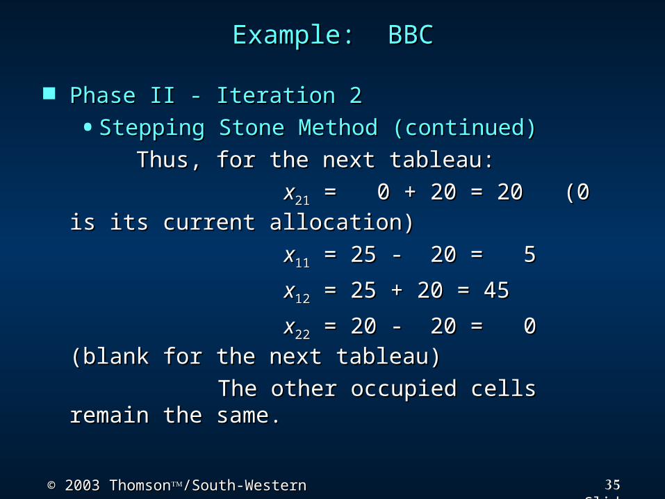
•Stepping Stone Method (continued)Stepping Stone Method (continued)Thus, for the next tableau:Thus, for the next tableau:
xx2121 = 0 + 20 = 20 (0 is its current = 0 + 20 = 20 (0 is its current allocation)allocation)
xx1111 = 25 - 20 = 5 = 25 - 20 = 5 xx1212 = 25 + 20 = 45 = 25 + 20 = 45 xx2222 = 20 - 20 = 0 (blank for the next = 20 - 20 = 0 (blank for the next
tableau)tableau) The other occupied cells remain the same.The other occupied cells remain the same.
36© 2003 Thomson© 2003 Thomson/South-Western/South-Western Slide
Example: BBCExample: BBC Phase II - Iteration 3Phase II - Iteration 3
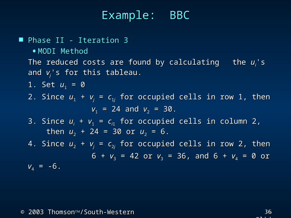
•MODI MethodMODI MethodThe reduced costs are found by calculating The reduced costs are found by calculating the the uuii's 's and and vvjj's for this tableau.'s for this tableau.1. Set 1. Set uu11 = 0 = 02. Since 2. Since uu11 + + vvjj = = cc11jj for occupied cells in row 1, then for occupied cells in row 1, then
vv11 = 24 and = 24 and vv22 = 30. = 30.3. Since 3. Since uuii + + vv11 = = ccii11 for occupied cells in column 2, for occupied cells in column 2, then then uu22 + 24 = 30 or + 24 = 30 or uu22 = 6. = 6. 4. Since 4. Since uu22 + + vvjj = = cc22jj for occupied cells in row 2, then for occupied cells in row 2, then
6 + 6 + vv33 = 42 or = 42 or vv33 = 36, and 6 + = 36, and 6 + vv44 = 0 or = 0 or vv44 = - = -6. 6.
37© 2003 Thomson© 2003 Thomson/South-Western/South-Western Slide
Example: BBCExample: BBC Phase II - Iteration 3Phase II - Iteration 3
•MODI Method (continued)MODI Method (continued)Calculate the reduced costs (circled Calculate the reduced costs (circled
numbers on the numbers on the next slide) by next slide) by ccijij - - uuii + + vvjj..
Unoccupied CellUnoccupied Cell Reduced CostReduced Cost (1,3) (1,3) 40 - 0 - 36 = 4 40 - 0 - 36 = 4 (1,4) (1,4) 0 - 0 - (-6) 0 - 0 - (-6)
= 6= 6 (2,2) (2,2) 40 - 6 - 30 = 4 40 - 6 - 30 = 4
38© 2003 Thomson© 2003 Thomson/South-Western/South-Western Slide
Example: BBCExample: BBC Phase II - Iteration 3Phase II - Iteration 3
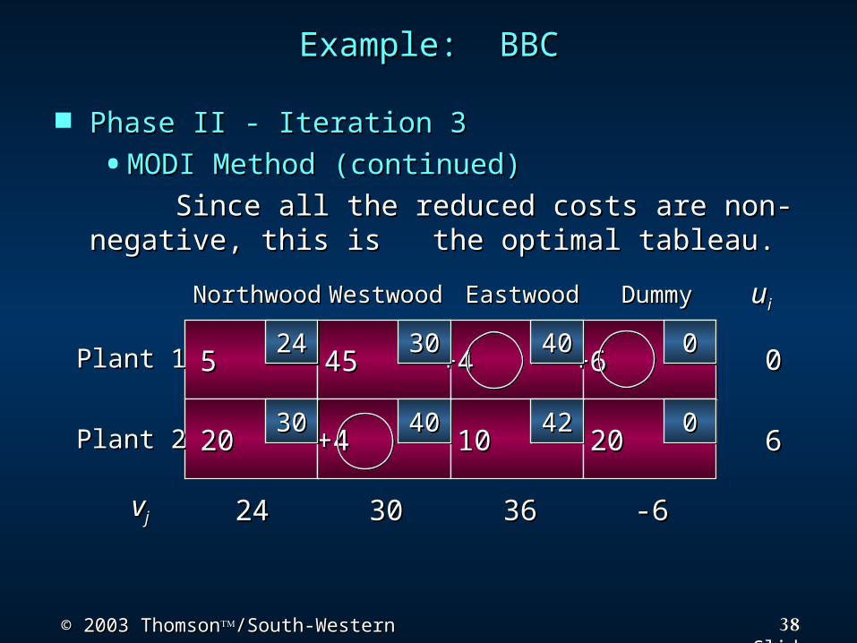
•MODI Method (continued)MODI Method (continued)Since all the reduced costs are non-Since all the reduced costs are non-
negative, this is negative, this is the optimal tableau.the optimal tableau.
55 45 45
20 20
+4 +4 +6 +6
+4 +4 10 10 20 20 4242
4040 00
004040
3030
3030
vvjj
uuii
66
00
-6-6363630302424
DummyDummy
Plant 1Plant 1
Plant 2Plant 2
EastwoodEastwoodWestwoodWestwoodNorthwoodNorthwood
2424
39© 2003 Thomson© 2003 Thomson/South-Western/South-Western Slide
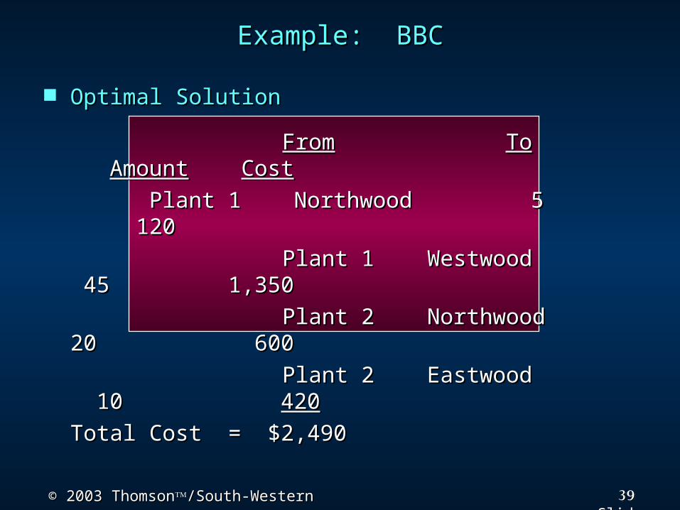
Example: BBCExample: BBC Optimal SolutionOptimal Solution FromFrom ToTo AmountAmount CostCost
Plant 1 Northwood 5 120Plant 1 Northwood 5 120 Plant 1 Westwood 45 1,350Plant 1 Westwood 45 1,350 Plant 2 Northwood 20 600Plant 2 Northwood 20 600 Plant 2 Eastwood 10 Plant 2 Eastwood 10 420420
Total Cost = $2,490Total Cost = $2,490
40© 2003 Thomson© 2003 Thomson/South-Western/South-Western Slide
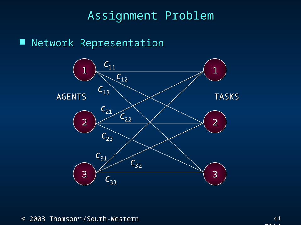
Assignment ProblemAssignment Problem An An assignment problemassignment problem seeks to minimize the seeks to minimize the
total cost assignment of total cost assignment of mm workers to workers to mm jobs, jobs, given that the cost of worker given that the cost of worker ii performing job performing job jj is is ccijij. .
It assumes all workers are assigned and each job It assumes all workers are assigned and each job is performed. is performed.
An assignment problem is a special case of a An assignment problem is a special case of a transportation problemtransportation problem in which all supplies and in which all supplies and all demands are equal to 1; hence assignment all demands are equal to 1; hence assignment problems may be solved as linear programs.problems may be solved as linear programs.
The The network representationnetwork representation of an assignment of an assignment problem with three workers and three jobs is problem with three workers and three jobs is shown on the next slide.shown on the next slide.
41© 2003 Thomson© 2003 Thomson/South-Western/South-Western Slide
Assignment ProblemAssignment Problem Network RepresentationNetwork Representation
22
33
11
22
33
11 cc1111cc1212
cc1313
cc2121 cc2222
cc2323
cc3131 cc3232
cc3333
AGENTSAGENTS TASKSTASKS
42© 2003 Thomson© 2003 Thomson/South-Western/South-Western Slide
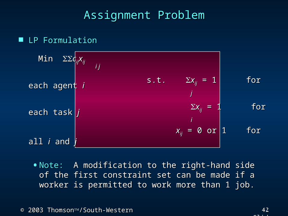
Assignment ProblemAssignment Problem LP FormulationLP Formulation
Min Min ccijijxxijij i ji j
s.t. s.t. xxijij = 1 for each agent = 1 for each agent ii jj xxijij = 1 for each task = 1 for each task jj ii xxijij = 0 or 1 for all = 0 or 1 for all ii and and jj
•Note:Note: A modification to the right-hand side of A modification to the right-hand side of the first constraint set can be made if a worker the first constraint set can be made if a worker is permitted to work more than 1 job.is permitted to work more than 1 job.
43© 2003 Thomson© 2003 Thomson/South-Western/South-Western Slide
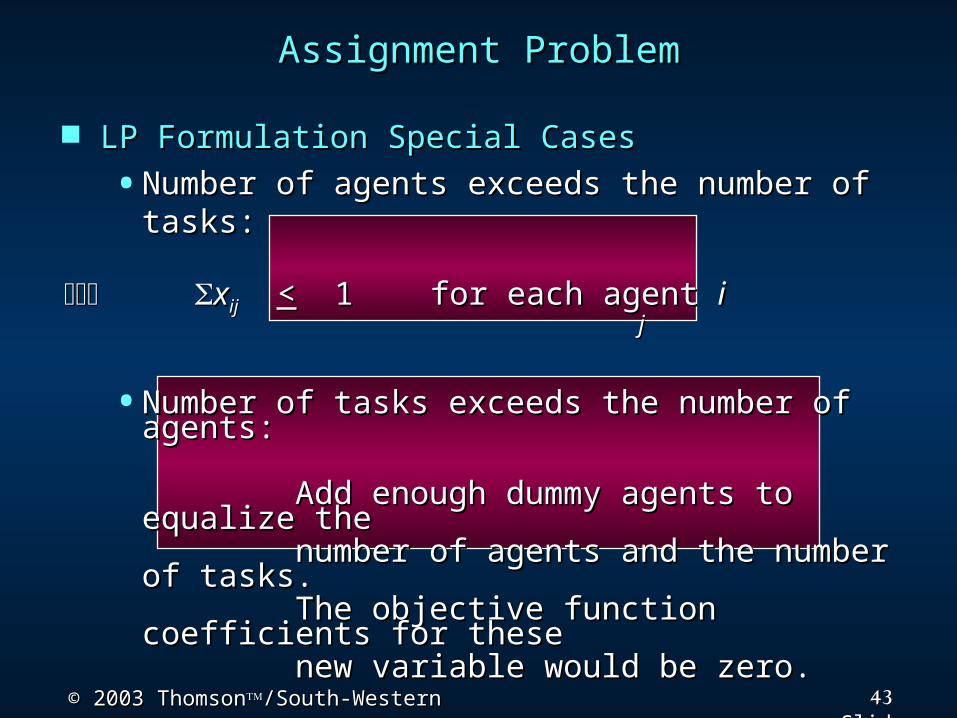
LP Formulation Special CasesLP Formulation Special Cases•Number of agents exceeds the number of Number of agents exceeds the number of
tasks:tasks:
xxijij << 1 for each agent 1 for each agent ii jj
•Number of tasks exceeds the number of Number of tasks exceeds the number of agents:agents: Add enough dummy agents to Add enough dummy agents to equalize theequalize the number of agents and the number of number of agents and the number of tasks.tasks. The objective function coefficients for The objective function coefficients for thesethese new variable would be zero.new variable would be zero.
Assignment ProblemAssignment Problem
44© 2003 Thomson© 2003 Thomson/South-Western/South-Western Slide
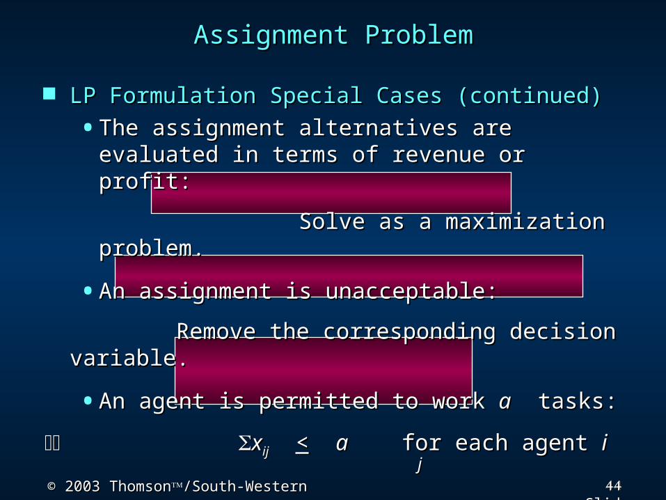
Assignment ProblemAssignment Problem LP Formulation Special Cases (continued)LP Formulation Special Cases (continued)
•The assignment alternatives are evaluated in The assignment alternatives are evaluated in terms of revenue or profit:terms of revenue or profit:
Solve as a maximization problem.Solve as a maximization problem.•An assignment is unacceptable:An assignment is unacceptable:
Remove the corresponding decision Remove the corresponding decision variable.variable.
•An agent is permitted to work An agent is permitted to work aa tasks: tasks:xxijij << aa for each agent for each agent ii jj
45© 2003 Thomson© 2003 Thomson/South-Western/South-Western Slide
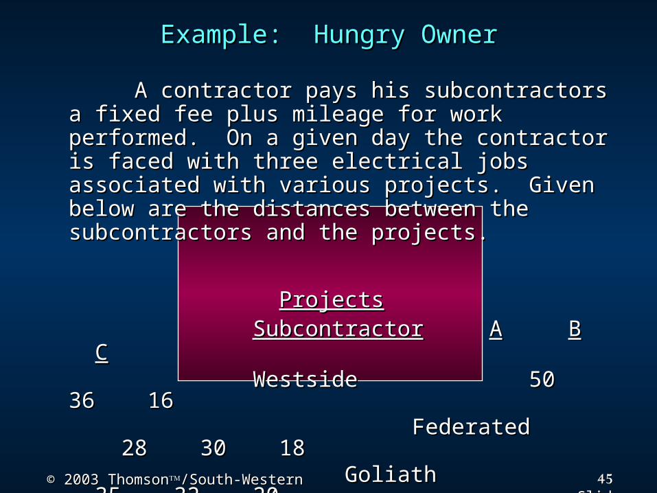
A contractor pays his subcontractors a A contractor pays his subcontractors a fixed fee plus mileage for work performed. On a fixed fee plus mileage for work performed. On a given day the contractor is faced with three given day the contractor is faced with three electrical jobs associated with various projects. electrical jobs associated with various projects. Given below are the distances between the Given below are the distances between the subcontractors and the projects.subcontractors and the projects.
ProjectsProjects SubcontractorSubcontractor AA BB CC Westside 50 36 16Westside 50 36 16
Federated 28 30 18 Federated 28 30 18 Goliath 35 32 20Goliath 35 32 20
Universal 25 25 14Universal 25 25 14How should the contractors be assigned to How should the contractors be assigned to minimize total costs?minimize total costs?
Example: Hungry OwnerExample: Hungry Owner
46© 2003 Thomson© 2003 Thomson/South-Western/South-Western Slide
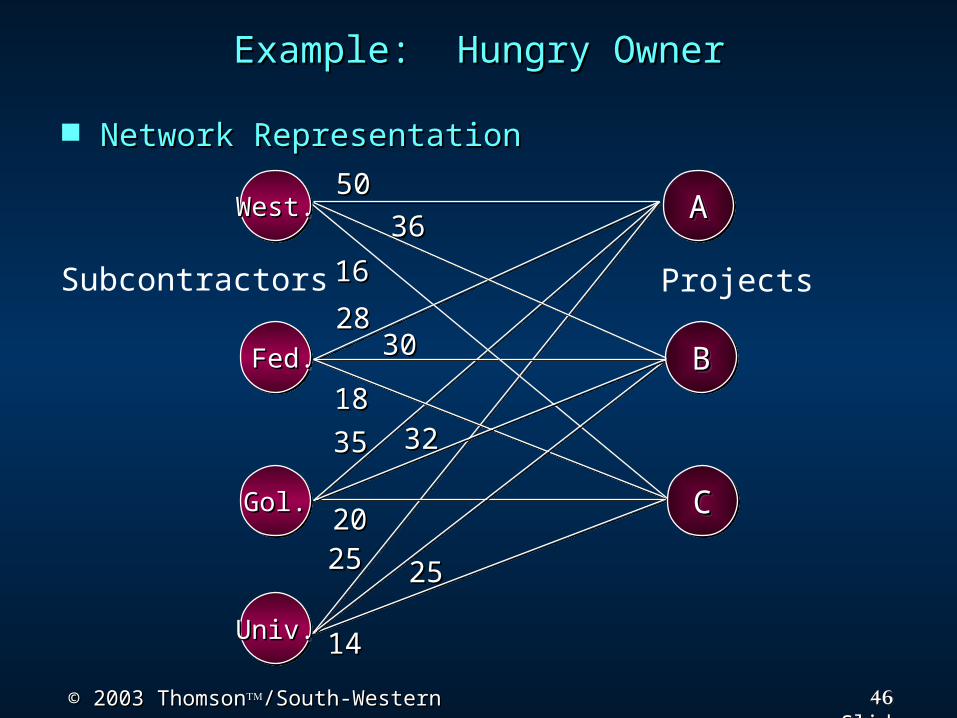
Example: Hungry OwnerExample: Hungry Owner Network RepresentationNetwork Representation
50503636
16162828
303018183535 3232
20202525 2525
1414
WestWest..
CC
BB
AA
Univ.Univ.
Gol.Gol.
Fed.Fed.
ProjectsSubcontractors
47© 2003 Thomson© 2003 Thomson/South-Western/South-Western Slide
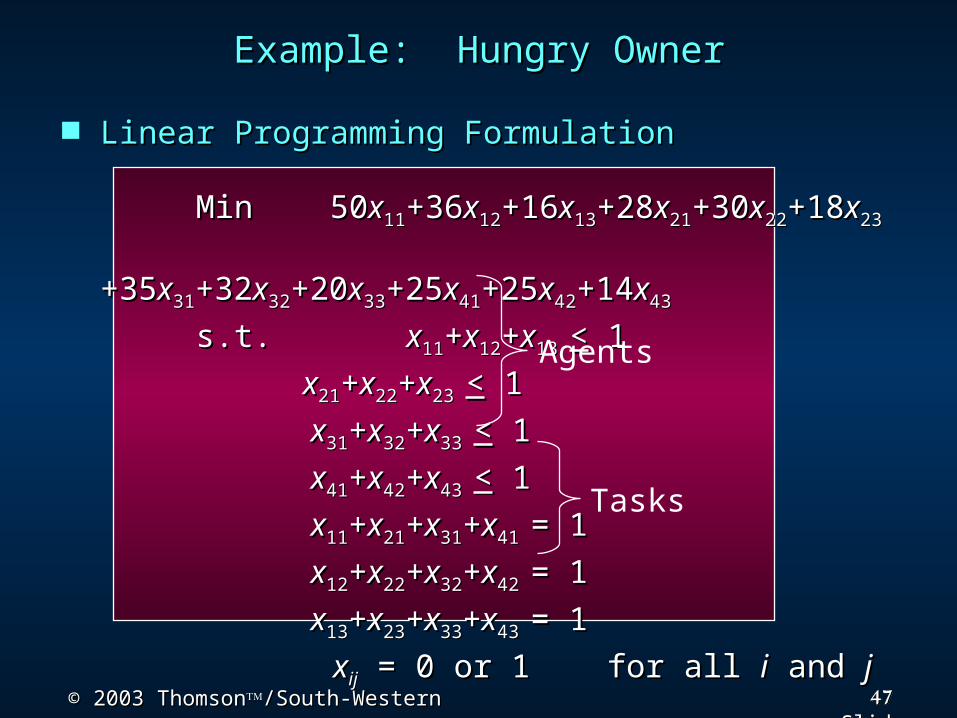
Example: Hungry OwnerExample: Hungry Owner Linear Programming FormulationLinear Programming Formulation
Min 50Min 50xx1111+36+36xx1212+16+16xx1313+28+28xx2121+30+30xx2222+18+18xx2323
+35+35xx3131+32+32xx3232+20+20xx3333+25+25xx4141+25+25xx4242+14+14xx4343
s.t. s.t. xx1111++xx1212++xx13 13 << 1 1 xx2121++xx2222++xx23 23 << 1 1 xx3131++xx3232++xx33 33 << 1 1 xx4141++xx4242++xx43 43 << 1 1 xx1111++xx2121++xx3131++xx41 41 = 1= 1 xx1212++xx2222++xx3232++xx42 42 = 1= 1 xx1313++xx2323++xx3333++xx43 43 = 1= 1 xxijij = 0 or 1 for all = 0 or 1 for all ii and and jj
Agents
Tasks
48© 2003 Thomson© 2003 Thomson/South-Western/South-Western Slide
Hungarian MethodHungarian Method The The Hungarian methodHungarian method solves minimization solves minimization
assignment problems with assignment problems with mm workers and workers and mm jobs. jobs.
Special considerations can include:Special considerations can include:•number of workers does not equal the number number of workers does not equal the number
of jobs -- add dummy workers or jobs with 0 of jobs -- add dummy workers or jobs with 0 assignment costs as neededassignment costs as needed
•worker worker ii cannot do job cannot do job jj -- assign -- assign ccijij = + = +MM•maximization objective -- create an maximization objective -- create an
opportunity loss matrixopportunity loss matrix subtracting all profits subtracting all profits for each job from the maximum profit for that for each job from the maximum profit for that job before beginning the Hungarian methodjob before beginning the Hungarian method
49© 2003 Thomson© 2003 Thomson/South-Western/South-Western Slide
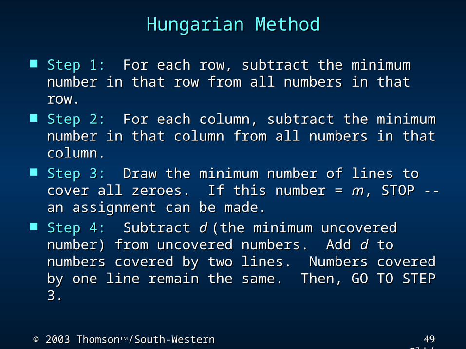
Hungarian MethodHungarian Method Step 1:Step 1: For each row, subtract the minimum For each row, subtract the minimum
number in that row from all numbers in that row.number in that row from all numbers in that row. Step 2:Step 2: For each column, subtract the minimum For each column, subtract the minimum
number in that column from all numbers in that number in that column from all numbers in that column. column.
Step 3:Step 3: Draw the minimum number of lines to Draw the minimum number of lines to cover all zeroes. If this number = cover all zeroes. If this number = mm, STOP -- an , STOP -- an assignment can be made.assignment can be made.
Step 4:Step 4: Subtract Subtract d d (the minimum uncovered (the minimum uncovered number) from uncovered numbers. Add number) from uncovered numbers. Add dd to to numbers covered by two lines. Numbers covered numbers covered by two lines. Numbers covered by one line remain the same. Then, GO TO STEP 3.by one line remain the same. Then, GO TO STEP 3.
50© 2003 Thomson© 2003 Thomson/South-Western/South-Western Slide
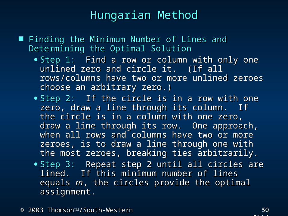
Hungarian MethodHungarian Method Finding the Minimum Number of Lines and Finding the Minimum Number of Lines and
Determining the Optimal SolutionDetermining the Optimal Solution•Step 1:Step 1: Find a row or column with only one Find a row or column with only one
unlined zero and circle it. (If all rows/columns unlined zero and circle it. (If all rows/columns have two or more unlined zeroes choose an have two or more unlined zeroes choose an arbitrary zero.)arbitrary zero.)
•Step 2:Step 2: If the circle is in a row with one zero, If the circle is in a row with one zero, draw a line through its column. If the circle is in a draw a line through its column. If the circle is in a column with one zero, draw a line through its row. column with one zero, draw a line through its row. One approach, when all rows and columns have One approach, when all rows and columns have two or more zeroes, is to draw a line through one two or more zeroes, is to draw a line through one with the most zeroes, breaking ties arbitrarily.with the most zeroes, breaking ties arbitrarily.
•Step 3:Step 3: Repeat step 2 until all circles are lined. If Repeat step 2 until all circles are lined. If this minimum number of lines equals this minimum number of lines equals mm, the , the circles provide the optimal assignment.circles provide the optimal assignment.
51© 2003 Thomson© 2003 Thomson/South-Western/South-Western Slide
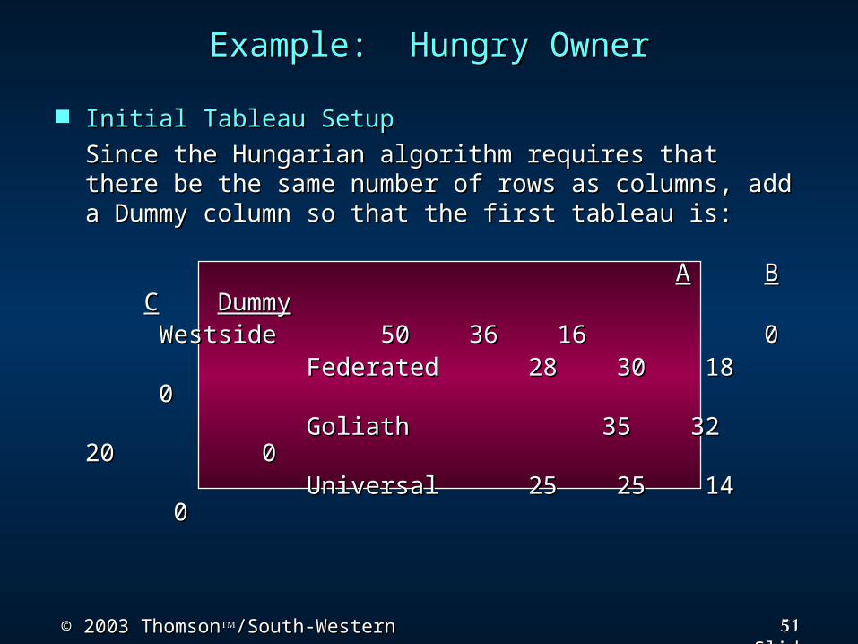
Example: Hungry OwnerExample: Hungry Owner Initial Tableau SetupInitial Tableau Setup
Since the Hungarian algorithm requires that there be Since the Hungarian algorithm requires that there be the same number of rows as columns, add a Dummy the same number of rows as columns, add a Dummy column so that the first tableau is:column so that the first tableau is:
AA BB CC DummyDummy Westside Westside 50 36 16 50 36 16 0 0
Federated Federated 28 30 18 028 30 18 0 Goliath Goliath 35 32 20 035 32 20 0 Universal Universal 25 25 14 25 25 14 0 0
52© 2003 Thomson© 2003 Thomson/South-Western/South-Western Slide
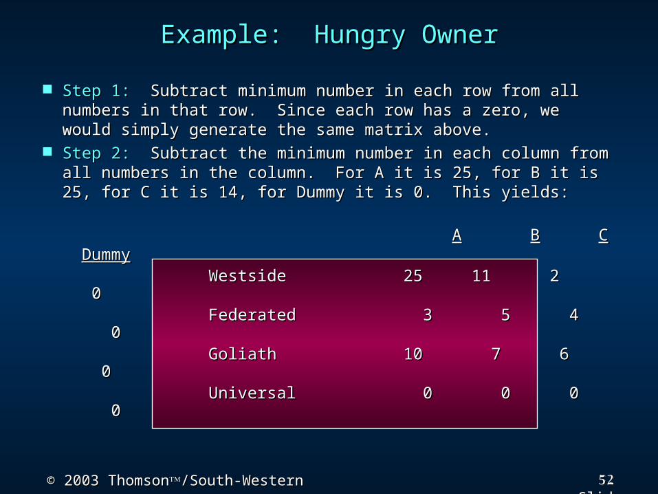
Example: Hungry OwnerExample: Hungry Owner Step 1:Step 1: Subtract minimum number in each row from Subtract minimum number in each row from
all numbers in that row. Since each row has a zero, all numbers in that row. Since each row has a zero, we would simply generate the same matrix above.we would simply generate the same matrix above.
Step 2:Step 2: Subtract the minimum number in each Subtract the minimum number in each column from all numbers in the column. For A it is column from all numbers in the column. For A it is 25, for B it is 25, for C it is 14, for Dummy it is 0. This 25, for B it is 25, for C it is 14, for Dummy it is 0. This yields:yields:
AA BB CC DummyDummy Westside Westside 25 11 2 025 11 2 0 Federated Federated 3 5 4 0 3 5 4 0 Goliath Goliath 10 7 6 10 7 6 00 Universal Universal 0 0 0 0 0 0 0 0
53© 2003 Thomson© 2003 Thomson/South-Western/South-Western Slide
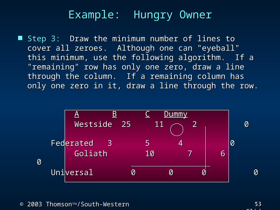
Example: Hungry OwnerExample: Hungry Owner Step 3:Step 3: Draw the minimum number of lines to Draw the minimum number of lines to
cover all zeroes. Although one can "eyeball" this cover all zeroes. Although one can "eyeball" this minimum, use the following algorithm. If a minimum, use the following algorithm. If a "remaining" row has only one zero, draw a line "remaining" row has only one zero, draw a line through the column. If a remaining column has through the column. If a remaining column has only one zero in it, draw a line through the row. only one zero in it, draw a line through the row.
AA BB CC DummyDummy WestsideWestside 25 11 2 0 25 11 2 0
FederatedFederated 3 5 4 0 3 5 4 0 Goliath Goliath 10 7 6 0 10 7 6 0 Universal Universal 0 0 0 0 0 0 0 0
54© 2003 Thomson© 2003 Thomson/South-Western/South-Western Slide
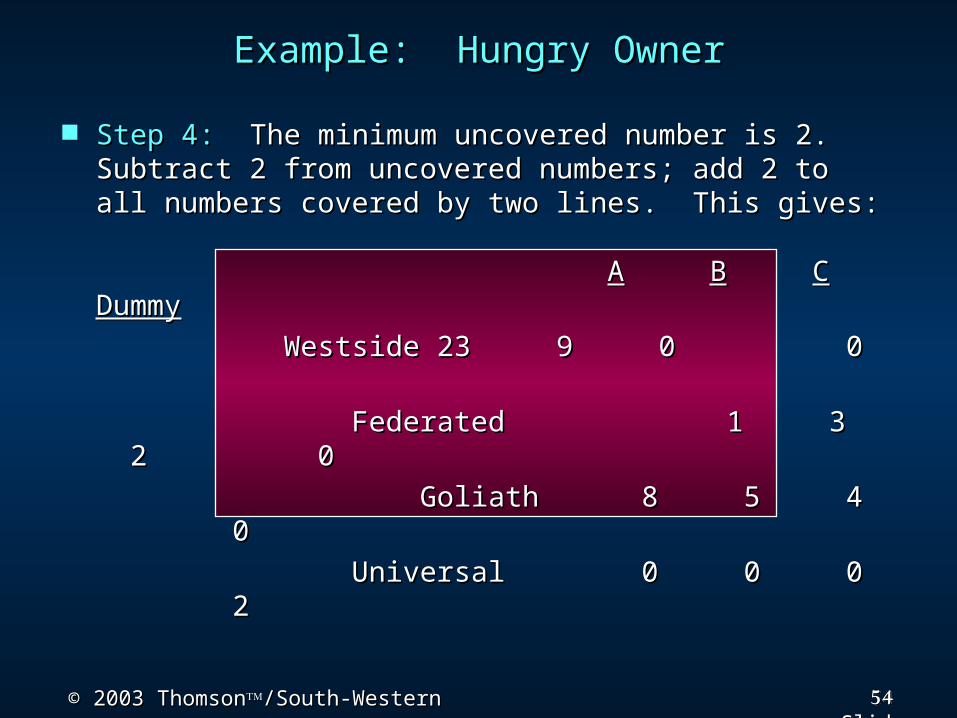
Step 4:Step 4: The minimum uncovered number is 2. The minimum uncovered number is 2. Subtract 2 from uncovered numbers; add 2 to all Subtract 2 from uncovered numbers; add 2 to all numbers covered by two lines. This gives:numbers covered by two lines. This gives:
AA BB CC DummyDummy WestsideWestside 23 9 0 0 23 9 0 0
Federated Federated 1 3 2 0 1 3 2 0
Goliath Goliath 8 5 4 0 8 5 4 0 Universal Universal 0 0 0 2 0 0 0 2
Example: Hungry OwnerExample: Hungry Owner
55© 2003 Thomson© 2003 Thomson/South-Western/South-Western Slide
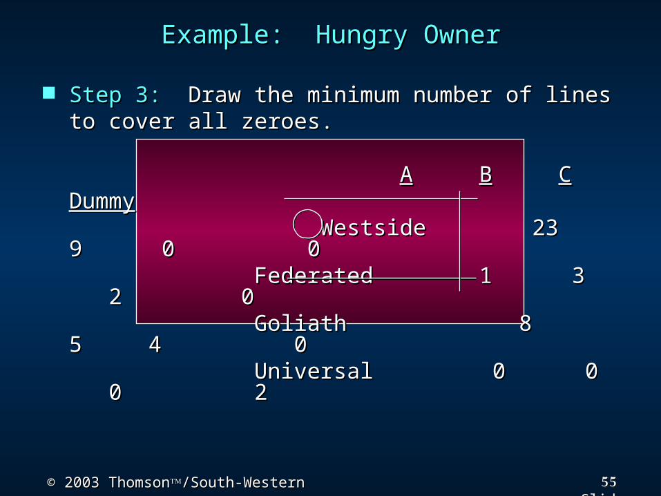
Example: Hungry OwnerExample: Hungry Owner Step 3:Step 3: Draw the minimum number of lines to Draw the minimum number of lines to
cover all zeroes.cover all zeroes.
AA BB CC DummyDummy Westside 23 9 0 0 Westside 23 9 0 0
Federated 1 3 2 0 Federated 1 3 2 0 Goliath 8 5 4 0 Goliath 8 5 4 0 Universal 0 0 0 2Universal 0 0 0 2
56© 2003 Thomson© 2003 Thomson/South-Western/South-Western Slide
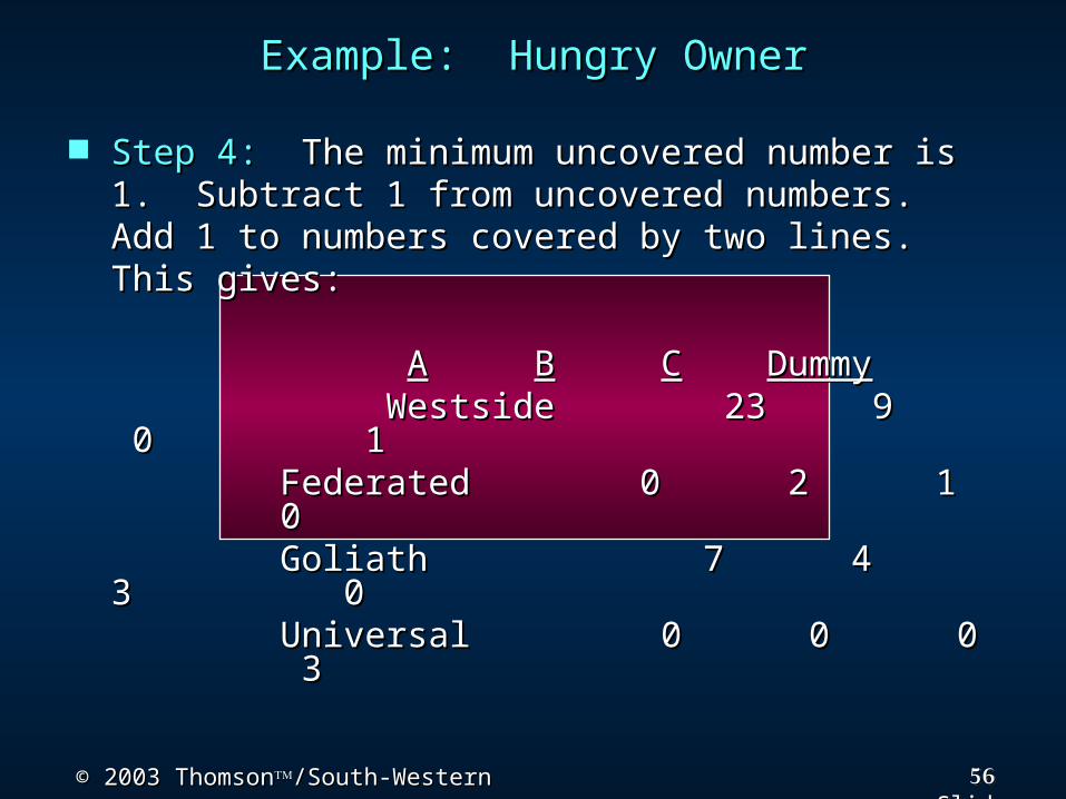
Example: Hungry OwnerExample: Hungry Owner Step 4:Step 4: The minimum uncovered number is 1. The minimum uncovered number is 1.
Subtract 1 from uncovered numbers. Add 1 to Subtract 1 from uncovered numbers. Add 1 to numbers covered by two lines. This gives:numbers covered by two lines. This gives:
AA BB CC DummyDummy Westside 23 9 0 1 Westside 23 9 0 1
Federated 0 2 1 0 Federated 0 2 1 0 Goliath 7 4 3 0 Goliath 7 4 3 0 Universal 0 0 0 3Universal 0 0 0 3
57© 2003 Thomson© 2003 Thomson/South-Western/South-Western Slide
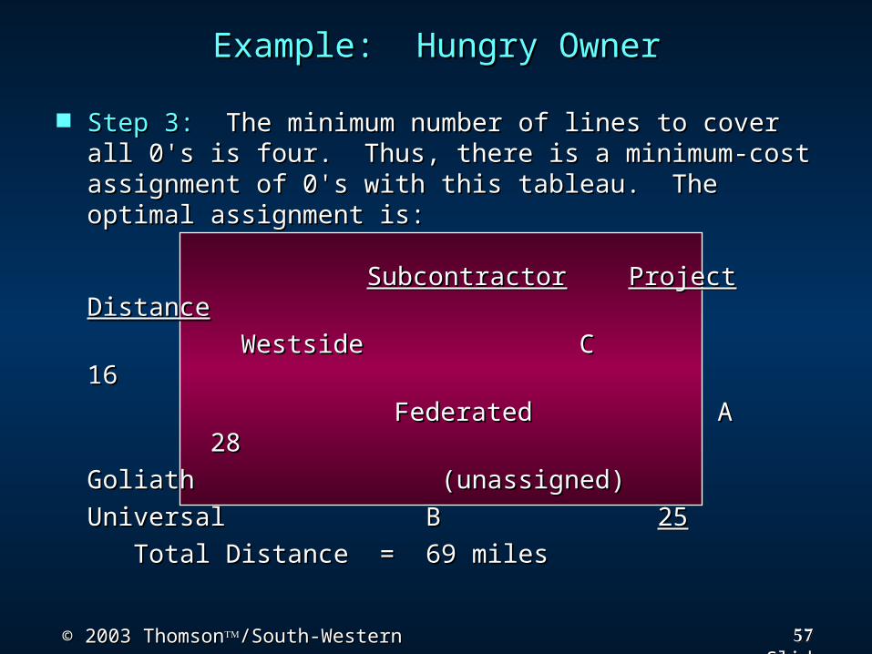
Example: Hungry OwnerExample: Hungry Owner Step 3:Step 3: The minimum number of lines to cover The minimum number of lines to cover
all 0's is four. Thus, there is a minimum-cost all 0's is four. Thus, there is a minimum-cost assignment of 0's with this tableau. The optimal assignment of 0's with this tableau. The optimal assignment is:assignment is:
SubcontractorSubcontractor ProjectProject DistanceDistance Westside C 16Westside C 16
Federated A 28Federated A 28Goliath (unassigned) Goliath (unassigned) Universal B Universal B 2525
Total Distance = 69 miles Total Distance = 69 miles
58© 2003 Thomson© 2003 Thomson/South-Western/South-Western Slide
Transshipment ProblemTransshipment Problem Transshipment problemsTransshipment problems are transportation are transportation
problems in which a shipment may move through problems in which a shipment may move through intermediate nodes (transshipment nodes)before intermediate nodes (transshipment nodes)before reaching a particular destination node.reaching a particular destination node.
Transshipment problems can be converted to Transshipment problems can be converted to larger transportation problems and solved by a larger transportation problems and solved by a special transportation program.special transportation program.
Transshipment problems can also be solved by Transshipment problems can also be solved by general purpose linear programming codes.general purpose linear programming codes.
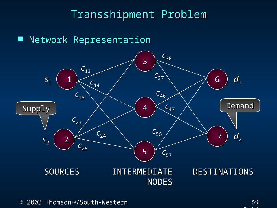
The network representation for a transshipment The network representation for a transshipment problem with two sources, three intermediate problem with two sources, three intermediate nodes, and two destinations is shown on the next nodes, and two destinations is shown on the next slide.slide.
59© 2003 Thomson© 2003 Thomson/South-Western/South-Western Slide
Transshipment ProblemTransshipment Problem Network RepresentationNetwork Representation
22
33
44
55
66
77
11cc1313
cc1414
cc2323
cc2424
cc2525
cc1515
ss11
cc3636
cc3737
cc4646
cc4747
cc5656
cc5757
dd11
dd22
INTERMEDIATEINTERMEDIATE NODESNODES
SOURCESSOURCES DESTINATIONSDESTINATIONS
ss22
DemanDemanddSupplySupply
60© 2003 Thomson© 2003 Thomson/South-Western/South-Western Slide
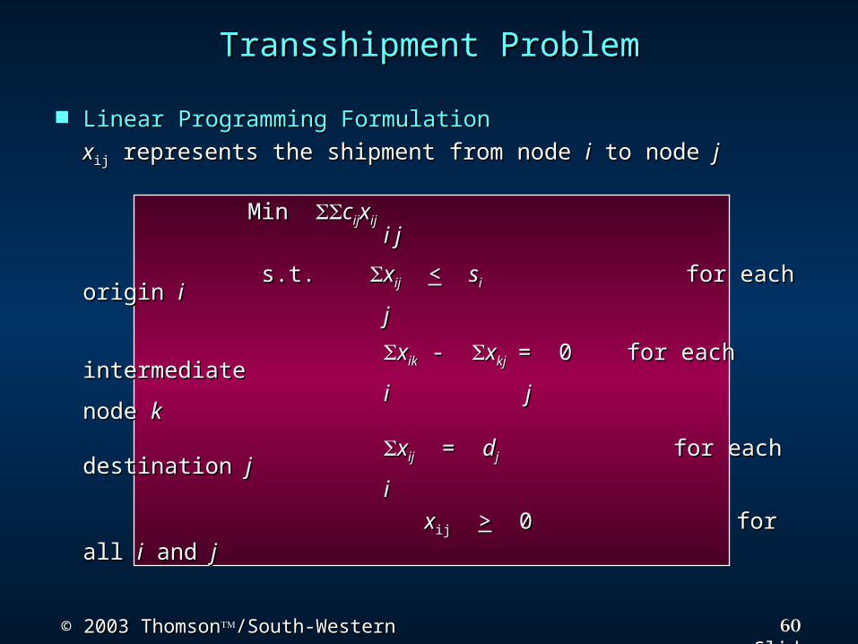
Transshipment ProblemTransshipment Problem Linear Programming FormulationLinear Programming Formulation xxijij represents the shipment from node represents the shipment from node ii to node to node jj
Min Min ccijijxxijij i ji j s.t. s.t. xxijij << ssii for each origin for each origin ii j j xxikik - - xxkjkj = 0 for each intermediate= 0 for each intermediate ii jj node node kk xxijij = = ddjj for each destination for each destination jj ii xxijij >> 0 for all 0 for all ii and and jj
61© 2003 Thomson© 2003 Thomson/South-Western/South-Western Slide
Example: TransshippingExample: Transshipping
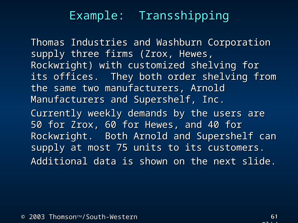
Thomas Industries and Washburn Thomas Industries and Washburn Corporation supply three firms (Zrox, Hewes, Corporation supply three firms (Zrox, Hewes, Rockwright) with customized shelving for its Rockwright) with customized shelving for its offices. They both order shelving from the same offices. They both order shelving from the same two manufacturers, Arnold Manufacturers and two manufacturers, Arnold Manufacturers and Supershelf, Inc. Supershelf, Inc.
Currently weekly demands by the users Currently weekly demands by the users are 50 for Zrox, 60 for Hewes, and 40 for are 50 for Zrox, 60 for Hewes, and 40 for Rockwright. Both Arnold and Supershelf can Rockwright. Both Arnold and Supershelf can supply at most 75 units to its customers. supply at most 75 units to its customers.
Additional data is shown on the next slide. Additional data is shown on the next slide.
62© 2003 Thomson© 2003 Thomson/South-Western/South-Western Slide
Example: TransshippingExample: Transshipping
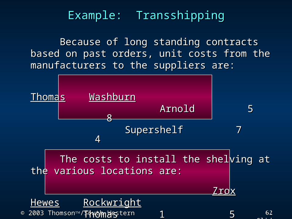
Because of long standing contracts based Because of long standing contracts based on past orders, unit costs from the on past orders, unit costs from the manufacturers to the suppliers are:manufacturers to the suppliers are:
ThomasThomas WashburnWashburn Arnold 5 8Arnold 5 8 Supershelf 7 4Supershelf 7 4
The costs to install the shelving at the The costs to install the shelving at the various locations are:various locations are:
ZroxZrox HewesHewes RockwrightRockwright Thomas 1 5 8Thomas 1 5 8
Washburn 3 4 4Washburn 3 4 4
63© 2003 Thomson© 2003 Thomson/South-Western/South-Western Slide
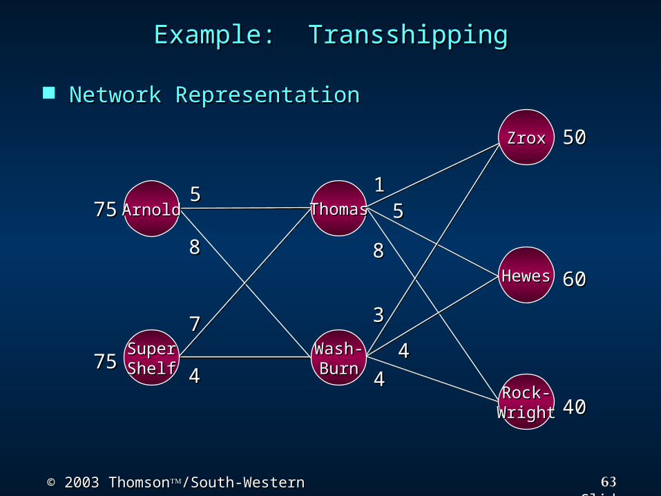
Example: TransshippingExample: Transshipping Network RepresentationNetwork Representation
ARNOLD
WASHBURN
ZROX
HEWES
7575
7575
5050
6060
4040
55
88
77
44
1155
88
3344
44
ArnoldArnold
SuperSuperShelfShelf
HewesHewes
ZroxZrox
ThomasThomas
Wash-Wash-BurnBurn
Rock-Rock-WrightWright
64© 2003 Thomson© 2003 Thomson/South-Western/South-Western Slide
Example: TransshippingExample: Transshipping Linear Programming FormulationLinear Programming Formulation
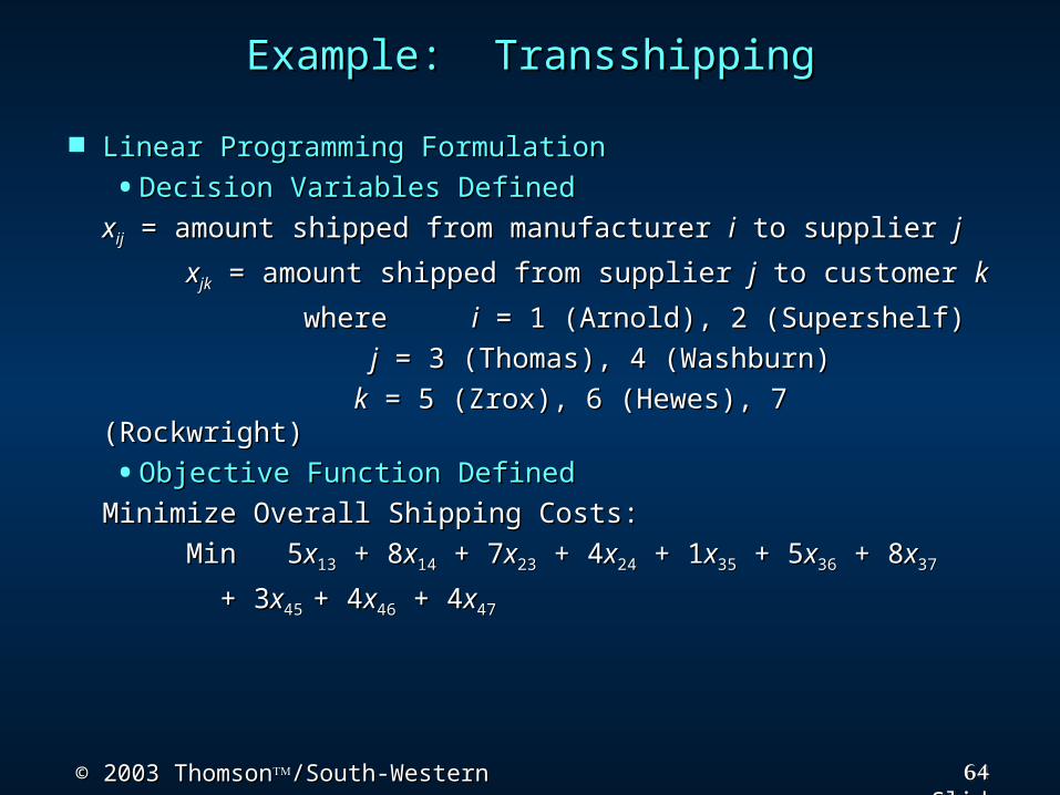
•Decision Variables DefinedDecision Variables Defined xxijij = amount shipped from manufacturer = amount shipped from manufacturer ii to supplier to supplier jj
xxjkjk = amount shipped from supplier = amount shipped from supplier jj to customer to customer kk where where ii = 1 (Arnold), 2 (Supershelf) = 1 (Arnold), 2 (Supershelf) jj = 3 (Thomas), 4 (Washburn) = 3 (Thomas), 4 (Washburn) kk = 5 (Zrox), 6 (Hewes), 7 (Rockwright) = 5 (Zrox), 6 (Hewes), 7 (Rockwright)
•Objective Function DefinedObjective Function DefinedMinimize Overall Shipping Costs: Minimize Overall Shipping Costs:
Min 5Min 5xx1313 + 8 + 8xx1414 + 7 + 7xx2323 + 4 + 4xx2424 + 1 + 1xx3535 + 5 + 5xx3636 + 8 + 8xx3737 + 3+ 3xx45 45 + 4+ 4xx4646 + 4 + 4xx4747
65© 2003 Thomson© 2003 Thomson/South-Western/South-Western Slide
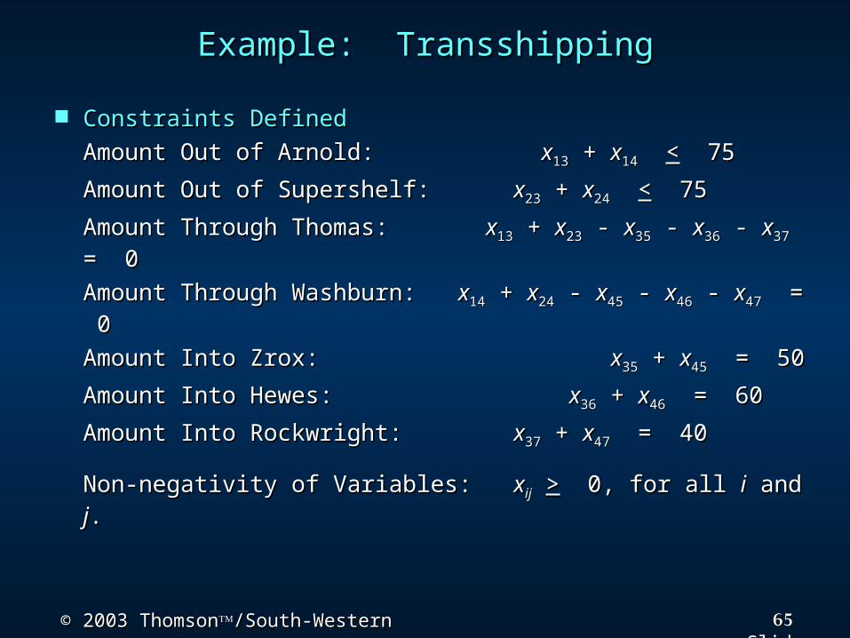
Example: TransshippingExample: Transshipping Constraints DefinedConstraints Defined
Amount Out of Arnold: Amount Out of Arnold: xx1313 + + xx1414 << 75 75Amount Out of Supershelf: Amount Out of Supershelf: xx2323 + + xx2424 << 75 75Amount Through Thomas: Amount Through Thomas: xx1313 + + xx2323 - - xx3535 - - xx3636 - - xx3737 = 0= 0Amount Through Washburn: Amount Through Washburn: xx1414 + + xx2424 - - xx4545 - - xx4646 - - xx4747 = 0= 0Amount Into Zrox: Amount Into Zrox: xx3535 + + xx4545 = 50 = 50Amount Into Hewes: Amount Into Hewes: xx3636 + + xx4646 = 60 = 60Amount Into Rockwright: Amount Into Rockwright: xx3737 + + xx4747 = 40 = 40
Non-negativity of Variables: Non-negativity of Variables: xxijij >> 0, for all 0, for all ii and and jj..
66© 2003 Thomson© 2003 Thomson/South-Western/South-Western Slide
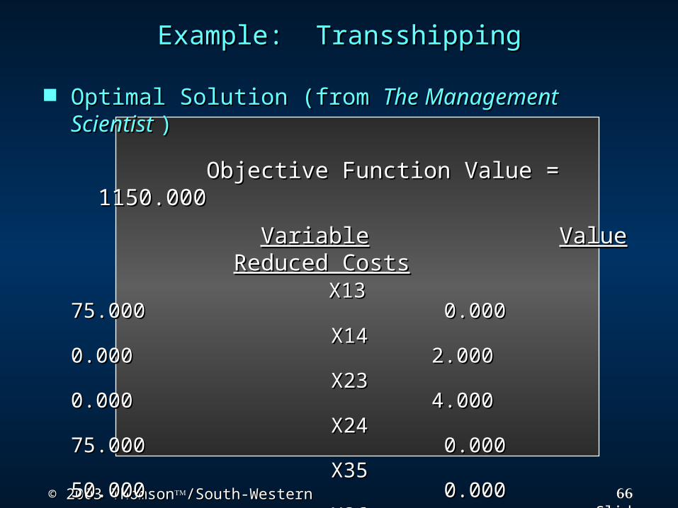
Example: TransshippingExample: Transshipping Optimal Solution (from Optimal Solution (from The Management The Management
Scientist Scientist )) Objective Function Value = Objective Function Value =
1150.0001150.000 VariableVariable ValueValue Reduced Reduced
CostsCosts X13 75.000 X13 75.000
0.0000.000 X14 0.000 X14 0.000
2.0002.000 X23 0.000 X23 0.000
4.0004.000 X24 75.000 X24 75.000
0.0000.000 X35 50.000 X35 50.000
0.0000.000 X36 25.000 X36 25.000
0.0000.000 X37 0.000 X37 0.000
3.0003.000 X45 0.000 X45 0.000
3.0003.000 X46 35.000 X46 35.000
0.0000.000 X47 40.000 X47 40.000
0.0000.000
67© 2003 Thomson© 2003 Thomson/South-Western/South-Western Slide
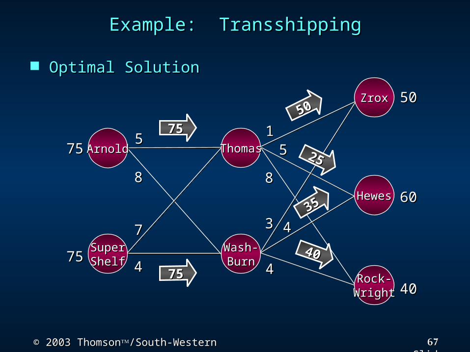
Example: TransshippingExample: Transshipping Optimal SolutionOptimal Solution
ARNOLD
WASHBURN
ZROX
HEWES
7575
7575
5050
6060
4040
55
88
77
44
1155
88
33 44
44
ArnoldArnold
SuperSuperShelfShelf
HewesHewes
ZroxZrox
ThomasThomas
Wash-Wash-BurnBurn
Rock-Rock-WrightWright
7575
7575
5050
2525
3535
4040
68© 2003 Thomson© 2003 Thomson/South-Western/South-Western Slide
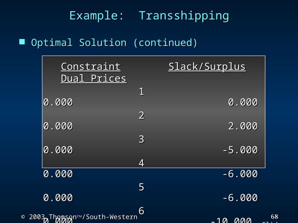
Example: TransshippingExample: Transshipping Optimal Solution (continued)Optimal Solution (continued)
ConstraintConstraint Slack/SurplusSlack/Surplus Dual Dual PricesPrices
1 0.000 1 0.000 0.000 0.000
2 0.000 2 0.000 2.000 2.000
3 0.000 3 0.000 -5.000-5.000
4 0.000 4 0.000 -6.000-6.000
5 0.000 5 0.000 -6.000-6.000
6 0.000 -6 0.000 -10.00010.000
7 0.000 -7 0.000 -10.00010.000
69© 2003 Thomson© 2003 Thomson/South-Western/South-Western Slide
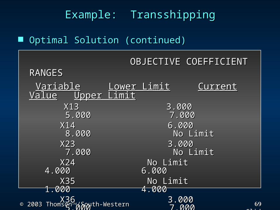
Example: TransshippingExample: Transshipping Optimal Solution (continued)Optimal Solution (continued)
OBJECTIVE COEFFICIENT RANGESOBJECTIVE COEFFICIENT RANGES VariableVariable Lower LimitLower Limit Current ValueCurrent Value Upper Upper
LimitLimit X13 3.000 5.000 X13 3.000 5.000
7.0007.000 X14 6.000 8.000 X14 6.000 8.000
No LimitNo Limit X23 3.000 7.000 X23 3.000 7.000
No LimitNo Limit X24 No Limit 4.000 X24 No Limit 4.000
6.0006.000 X35 No Limit 1.000 X35 No Limit 1.000
4.0004.000 X36 3.000 5.000 X36 3.000 5.000
7.0007.000 X37 5.000 8.000 X37 5.000 8.000
No LimitNo Limit X45 0.000 3.000 X45 0.000 3.000
No LimitNo Limit X46 2.000 4.000 X46 2.000 4.000
6.0006.000 X47 No Limit 4.000 X47 No Limit 4.000
7.0007.000
70© 2003 Thomson© 2003 Thomson/South-Western/South-Western Slide
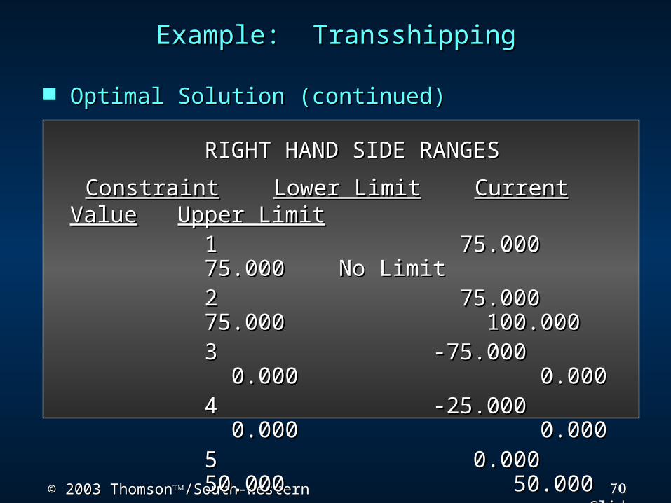
Example: TransshippingExample: Transshipping Optimal Solution (continued)Optimal Solution (continued)
RIGHT HAND SIDE RANGESRIGHT HAND SIDE RANGES ConstraintConstraint Lower LimitLower Limit Current ValueCurrent Value Upper Upper
LimitLimit 1 75.000 1 75.000 75.000 75.000
No LimitNo Limit 2 75.000 2 75.000 75.000 75.000
100.000 100.000 3 -75.000 3 -75.000 0.000 0.000
0.000 0.000 4 -25.000 4 -25.000 0.000 0.000
0.000 0.000 5 0.000 5 0.000 50.000 50.000
50.000 50.000 6 35.000 6 35.000 60.000 60.000
60.000 60.000 7 15.000 7 15.000 40.000 40.000
40.000 40.000
71© 2003 Thomson© 2003 Thomson/South-Western/South-Western Slide
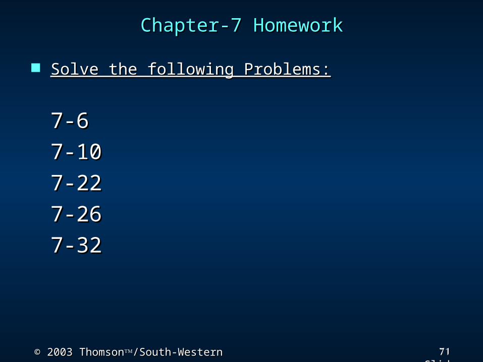
Chapter-7 HomeworkChapter-7 Homework Solve the following Problems:Solve the following Problems:
7-67-67-107-107-227-227-267-267-327-32
72© 2003 Thomson© 2003 Thomson/South-Western/South-Western Slide
The End of Chapter 7The End of Chapter 7


![ch07 [EDocFind.com]](https://img.pdfslide.tips/doc/110x75/577d2f341a28ab4e1eb116e2/ch07-edocfindcom.jpg)