Embed Size (px)
Citation preview
1
1 Chap.1 Introduction
CAE 기본개념 소개
Chap. 1 Introduction to FE Analysis
2 Chap.1 Introduction
CAE (Computer Aided Engineering)
CAE 정의
실생활에서 발생되는 여러 가지 물리적 현상을 예측하기 위해
컴퓨터 수치해석 기법을 통해 그 결과를 미리 Simulation하는 기법
CAE 해석기법 종류
유한요소법 (Finite Element Method; FEM)
유한차분법 (Finite Difference Method; FDM)
경계요소법 (Boundary Element Method: BEM)
유한체적법 (Finite Volume Method; FVM)
CAE 적용 분야
구조해석, 충돌해석, 열/유체 유동해석, 소음/진동 해석
각종 성형공정 해석(단조, 압출, 박판성형, 사출성형, 주조 등)
전자기장 해석, 광학계 해석, 분자구조 해석 등
2
3 Chap.1 Introduction
유한요소법 (Finite Element Method; FEM)
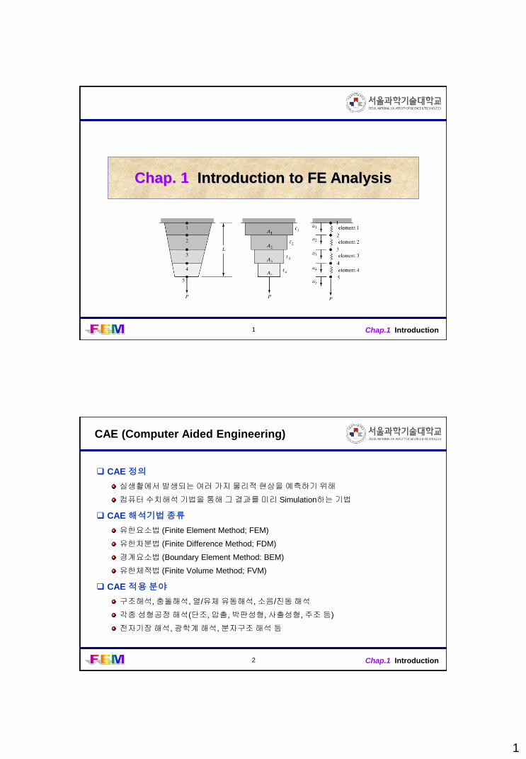
유한요소법 특징
지배방정식 (미분방정식) 적분 형태의 방정식 (variational principle)
연속체(continuum)로 정의된 전체 영역을 이산화(discretization)
: 다수개의 유한요소(finite element)로 구성 Mesh
각 요소 내에서 보간함수(interpolation function)를 사용하여 실제 결과를 근사화
실제 온도분포 (연속체) 유한요소 근사화 결과 (선형보간)
Error
4 Chap.1 Introduction
Engineering Problems
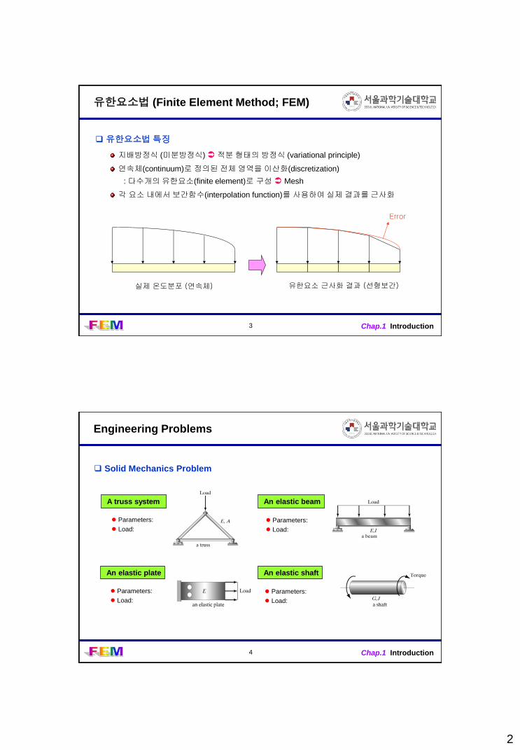
Solid Mechanics Problem
A truss system
Parameters:
Load:
An elastic beam
Parameters:
Load:
An elastic plate
Parameters:
Load:
An elastic shaft
Parameters:
Load:
3
5 Chap.1 Introduction
Engineering Problems
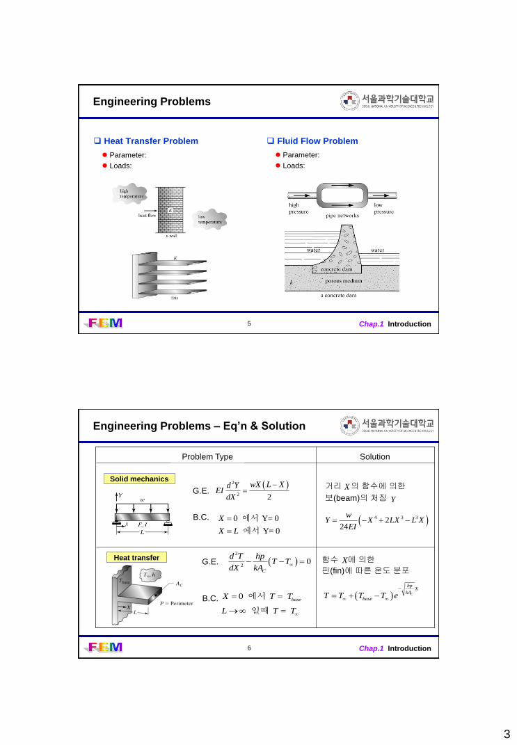
Heat Transfer Problem
Parameter:
Loads:
Fluid Flow Problem
Parameter:
Loads:
6 Chap.1 Introduction
Engineering Problems – Eq’n & Solution
Solution Problem Type
2
20
C
d T hpT T
dX kA G.E.
B.C. 0 baseX T T 에서
L T T 일때
C
hpX
kA
baseT T T T e
함수 에 의한
핀(fin)에 따른 온도 분포
X
m
Heat transfer
Solid mechanics 2
2 2
wX L Xd YEI
dX
G.E.
B.C. 0 Y= 0X 에서
Y= 0X L 에서 4 3 32
24
wY X LX L X
EI
거리 의 함수에 의한
보(beam)의 처짐
X
Y

4
7 Chap.1 Introduction
Engineering Problems – Eq’n & Solution
Ex) Simple compression of a rod
소재: 원형 봉재 (rod)
하중: 축방향 하중
재료의 위치(x)에 따른 변위(u)는?
기본 가정
재료의 단면은 일정함 (radius: r)
하중은 봉의 중심에 축방향으로 작용
재료는 선형 탄성재료로 가정
주변 온도는 균일하다고 가정 (iso-thermal)
등방성(isotropic) 재료로 가정
균일한(homogeneous) 재료로 가정
l
x E, r
F
8 Chap.1 Introduction
Engineering Problems – Eq’n & Solution
Ex 2) Simple compression of a rod
소재의 단면이 변하는 경우
하중: 축방향 하중
재료의 위치(x)에 따른 변위(u)는?
기본 가정
재료의 단면은 일정함 (radius: r)
하중은 봉의 중심에 축방향으로 작용
재료는 선형 탄성재료로 가정
주변 온도는 균일하다고 가정 (iso-thermal)
등방성(isotropic) 재료로 가정
균일한(homogeneous) 재료로 가정
l
x
r1
F
r2
5
9 Chap.1 Introduction
Numerical Methods
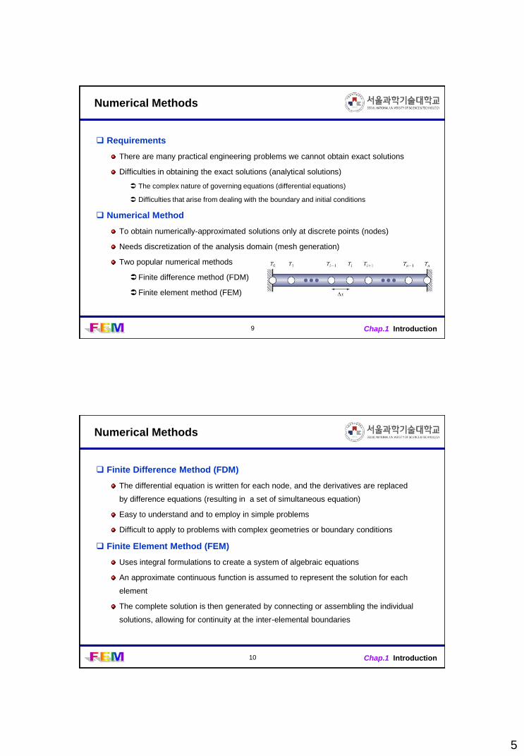
Requirements
There are many practical engineering problems we cannot obtain exact solutions
Difficulties in obtaining the exact solutions (analytical solutions)
The complex nature of governing equations (differential equations)
Difficulties that arise from dealing with the boundary and initial conditions
Numerical Method
To obtain numerically-approximated solutions only at discrete points (nodes)
Needs discretization of the analysis domain (mesh generation)
Two popular numerical methods
Finite difference method (FDM)
Finite element method (FEM)
10 Chap.1 Introduction
Numerical Methods
Finite Difference Method (FDM)
The differential equation is written for each node, and the derivatives are replaced
by difference equations (resulting in a set of simultaneous equation)
Easy to understand and to employ in simple problems
Difficult to apply to problems with complex geometries or boundary conditions
Finite Element Method (FEM)
Uses integral formulations to create a system of algebraic equations
An approximate continuous function is assumed to represent the solution for each
element
The complete solution is then generated by connecting or assembling the individual
solutions, allowing for continuity at the inter-elemental boundaries
6
11 Chap.1 Introduction
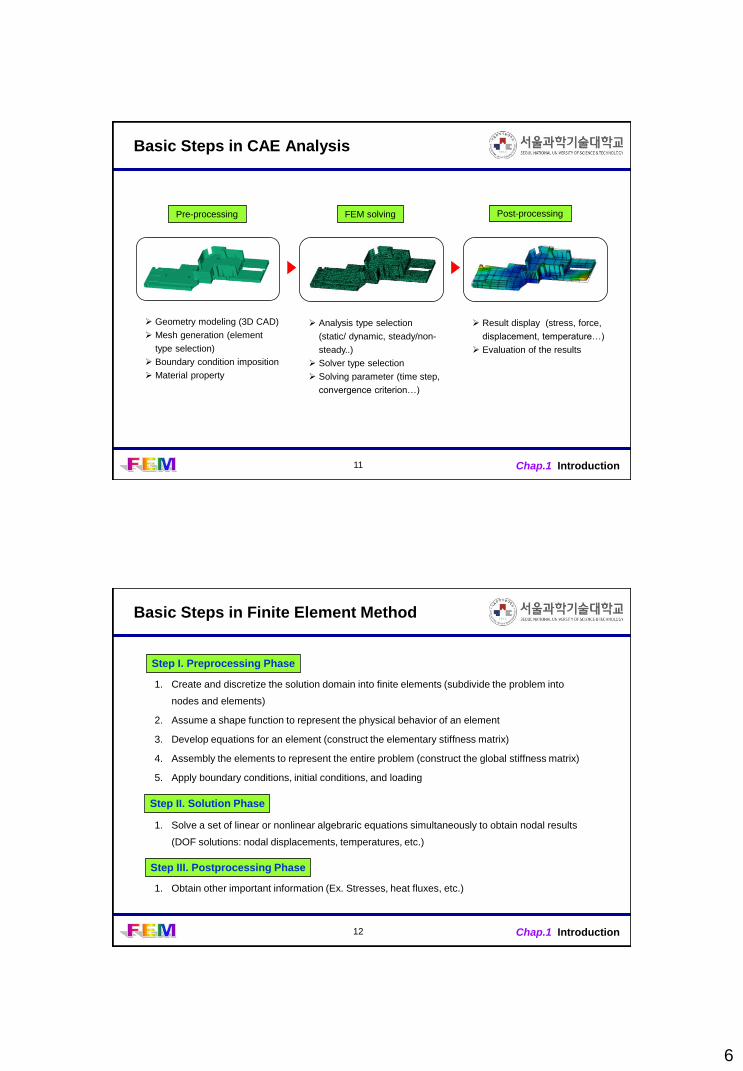
Basic Steps in CAE Analysis
Pre-processing FEM solving Post-processing
Geometry modeling (3D CAD)
Mesh generation (element
type selection)
Boundary condition imposition
Material property
Analysis type selection
(static/ dynamic, steady/non-
steady..)
Solver type selection
Solving parameter (time step,
convergence criterion…)
Result display (stress, force,
displacement, temperature…)
Evaluation of the results
12 Chap.1 Introduction
Basic Steps in Finite Element Method
1. Create and discretize the solution domain into finite elements (subdivide the problem into
nodes and elements)
2. Assume a shape function to represent the physical behavior of an element
3. Develop equations for an element (construct the elementary stiffness matrix)
4. Assembly the elements to represent the entire problem (construct the global stiffness matrix)
5. Apply boundary conditions, initial conditions, and loading
1. Solve a set of linear or nonlinear algebraric equations simultaneously to obtain nodal results
(DOF solutions: nodal displacements, temperatures, etc.)
1. Obtain other important information (Ex. Stresses, heat fluxes, etc.)
Step I. Preprocessing Phase
Step II. Solution Phase
Step III. Postprocessing Phase
7
13 Chap.1 Introduction
Finite Element Formulations
Direct Formulation
Follows the basic FEM steps (steps 1 ~ 7) as a direct manner
Ease to understand the basic FEM steps (not used in real FE formulation)
Minimum Total Potential Energy Formulation
A common approach in generating FE models in solid mechanics
Based on the strain energy during the deformation by the external forces
Weighted Residual Formulation
Based on assuming an approximate solution for the governing differential equation
The assumed solution leads to some errors (residuals)
To make these residuals vanish over some selected intervals or at some points
Collocation method, Subdomain method, Galerkin method, Least-square method)
14 Chap.1 Introduction
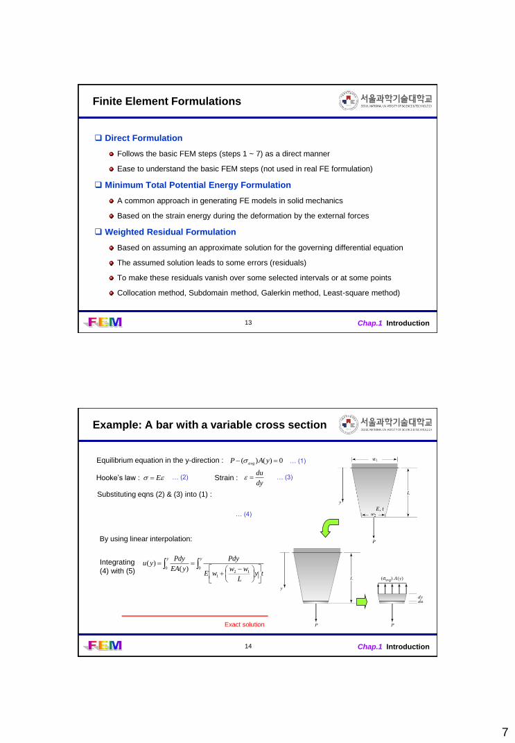
Example: A bar with a variable cross section
E, t
Equilibrium equation in the y-direction : 0)()( yAP avg
Hooke’s law : Strain : Edy
du
yy
tyL
wwwE
Pdy
yEA
Pdyyu
012
1
0 )()(
… (1)
… (2) … (3)
Substituting eqns (2) & (3) into (1) :
… (4)
By using linear interpolation:
Integrating
(4) with (5)
Exact solution
8
15 Chap.1 Introduction
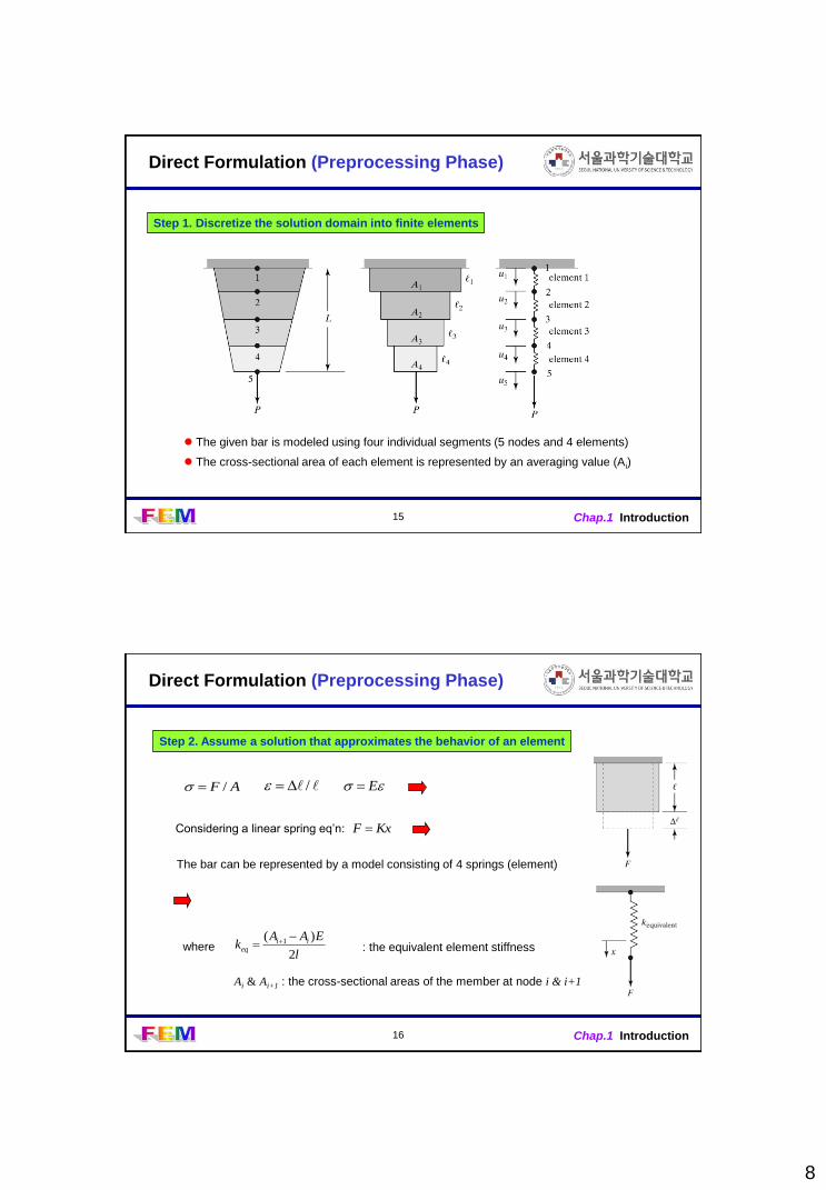
Direct Formulation (Preprocessing Phase)
Step 1. Discretize the solution domain into finite elements
The given bar is modeled using four individual segments (5 nodes and 4 elements)
The cross-sectional area of each element is represented by an averaging value (Ai)
16 Chap.1 Introduction
Direct Formulation (Preprocessing Phase)
Step 2. Assume a solution that approximates the behavior of an element
AF / / E
KxF Considering a linear spring eq’n:
The bar can be represented by a model consisting of 4 springs (element)
where : the equivalent element stiffness
Ai & Ai+1 : the cross-sectional areas of the member at node i & i+1
l
EAAk ii
eq2
)( 1
9
17 Chap.1 Introduction
Direct Formulation (Preprocessing Phase)
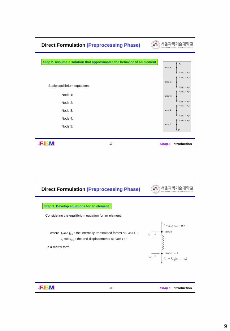
Step 2. Assume a solution that approximates the behavior of an element
Node 1:
Node 2:
Node 3:
Node 4:
Node 5:
Static equilibrium equations:
18 Chap.1 Introduction
Direct Formulation (Preprocessing Phase)
Step 3. Develop equations for an element
where fi and fi+1 : the internally transmitted forces at i and i+1
ui and ui+1 : the end displacements at i and i+1
Considering the equilibrium equation for an element:
In a matrix form,
10
19 Chap.1 Introduction
Direct Formulation (Preprocessing Phase)
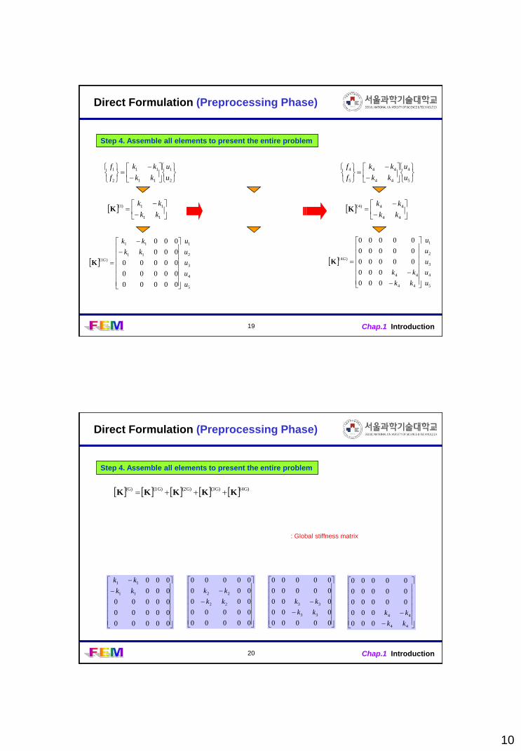
Step 4. Assemble all elements to present the entire problem
11
11)1(
kk
kkK
5
4
3
2
1
11
11
)1(
00000
00000
00000
000
000
u
u
u
u
u
kk
kk
G
K
44
44)4(
kk
kkK
5
4
3
2
1
44
44
)4(
000
000
00000
00000
00000
u
u
u
u
u
kk
kk
G
K
2
1
11
11
2
1
u
u
kk
kk
f
f
5
4
44
44
5
4
u
u
kk
kk
f
f
20 Chap.1 Introduction
Direct Formulation (Preprocessing Phase)
Step 4. Assemble all elements to present the entire problem
(4G)(3G)(2G)(1G)(G)KKKKK
00000
00000
00000
000
000
11
11
kk
kk
00000
00000
000
000
00000
22
22
kk
kk
44
44
000
000
00000
00000
00000
kk
kk
00000
000
000
00000
00000
33
33
kk
kk
: Global stiffness matrix
11
21 Chap.1 Introduction
Direct Formulation (Preprocessing Phase)
Step 5. Apply boundary conditions and loads
5
4
3
2
1
5
4
3
2
1
44
4433
3322
2211
11
000
00
00
00
000
f
f
f
f
f
u
u
u
u
u
kk
kkkk
kkkk
kkkk
kk
u1 = 0, f5 = P
}{}]{[ fuK
[K]: Stiffness matrix
{f}: load vector
{u}: solution vector
22 Chap.1 Introduction
Direct Formulation (Solution Phase)
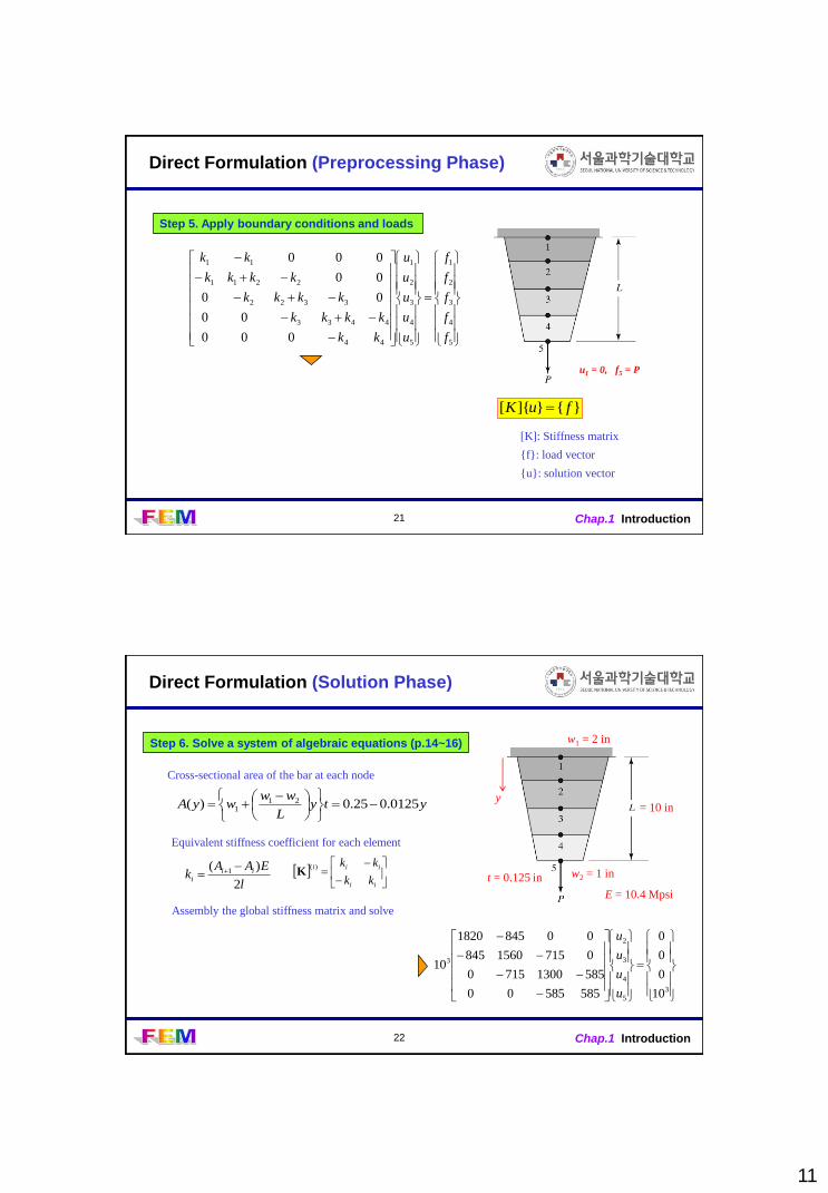
Step 6. Solve a system of algebraic equations (p.14~16)
ytyL
wwwyA 0125.025.0)( 21
1
l
EAAk ii
i2
)( 1
Cross-sectional area of the bar at each node
Equivalent stiffness coefficient for each element
w1 = 2 in
w2 = 1 in
y = 10 in
t = 0.125 in
E = 10.4 Mpsi
ii
iii
kk
kk)(K
Assembly the global stiffness matrix and solve
3
5
4
3
2
3
10
0
0
0
58558500
58513007150
07151560845
008451820
10
u
u
u
u
12
23 Chap.1 Introduction
Direct Formulation (Postprocessing Phase)
Step 7. Obtain other engineering information (p.16~18)
Average normal stresses in each element
Reaction forces at each node
0
0
0
0
1000
FuKR
lbuukR 1000)0001026.0(10975 3
1211
Reaction forces at each node
24 Chap.1 Introduction
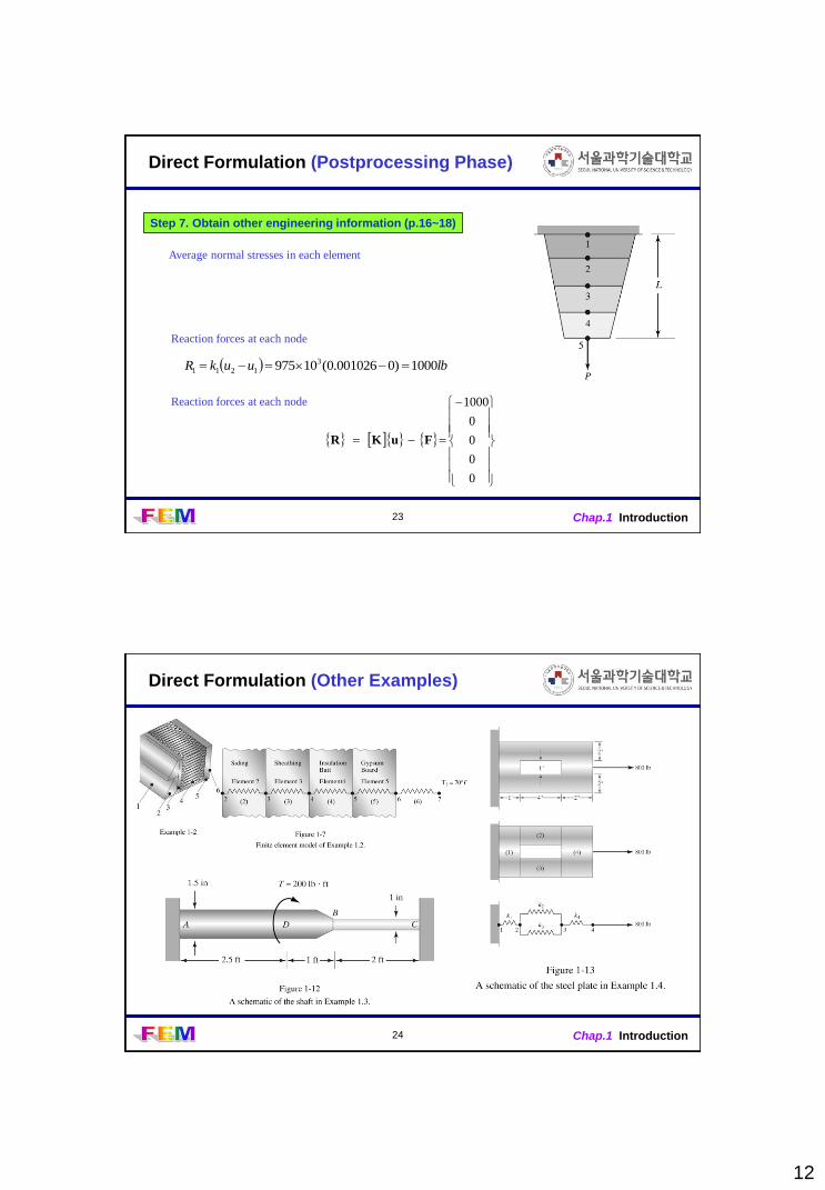
Direct Formulation (Other Examples)
13
25 Chap.1 Introduction
Minimum Total Potential Energy Formulation
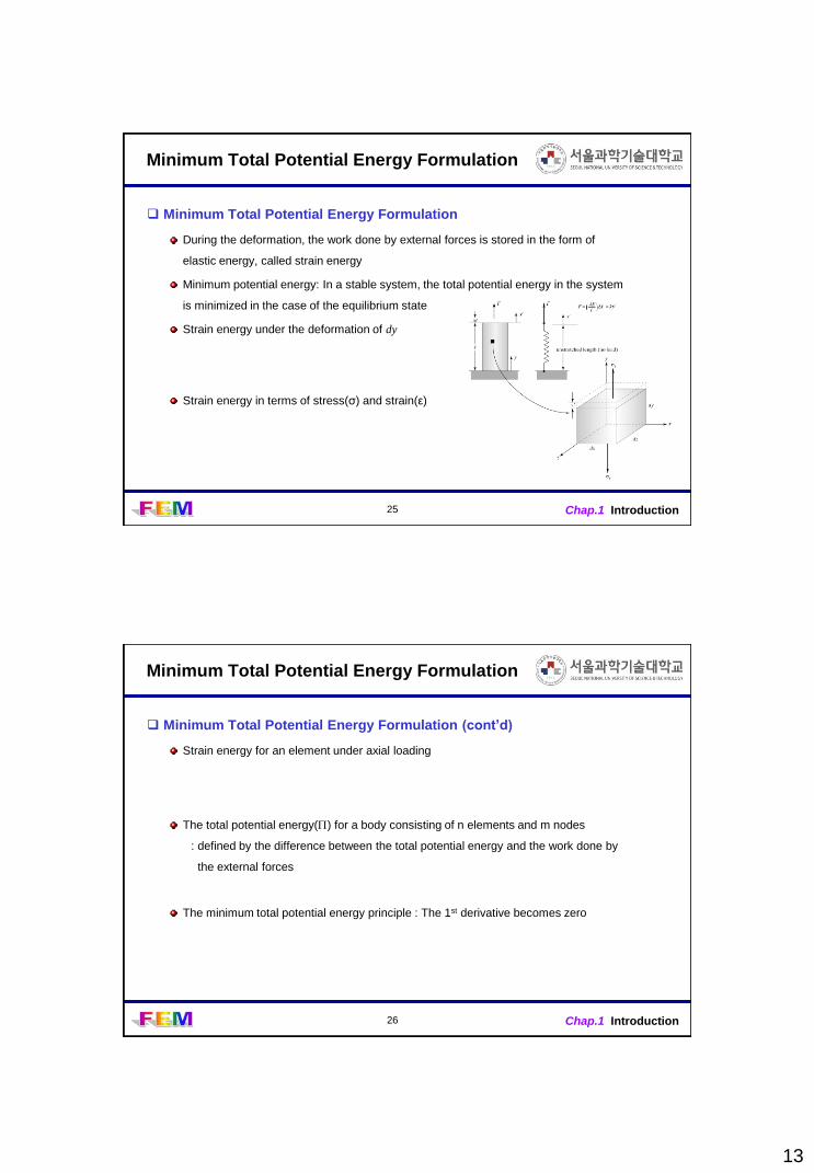
Minimum Total Potential Energy Formulation
During the deformation, the work done by external forces is stored in the form of
elastic energy, called strain energy
Minimum potential energy: In a stable system, the total potential energy in the system
is minimized in the case of the equilibrium state
Strain energy under the deformation of dy
Strain energy in terms of stress(σ) and strain(ε)
26 Chap.1 Introduction
Minimum Total Potential Energy Formulation
Minimum Total Potential Energy Formulation (cont’d)
Strain energy for an element under axial loading
The total potential energy() for a body consisting of n elements and m nodes
: defined by the difference between the total potential energy and the work done by
the external forces
The minimum total potential energy principle : The 1st derivative becomes zero
14
27 Chap.1 Introduction
Minimum Total Potential Energy Formulation
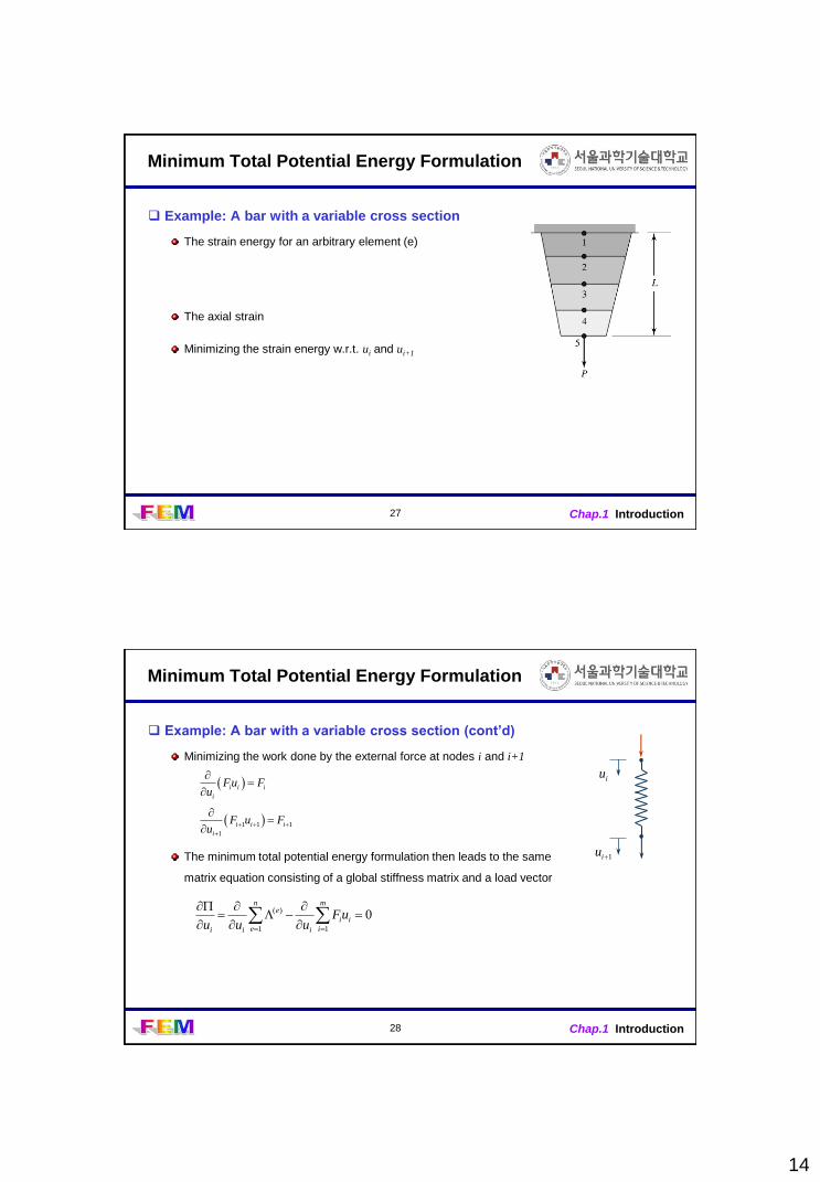
Example: A bar with a variable cross section
The strain energy for an arbitrary element (e)
The axial strain
Minimizing the strain energy w.r.t. ui and ui+1
28 Chap.1 Introduction
Minimum Total Potential Energy Formulation
Example: A bar with a variable cross section (cont’d)
Minimizing the work done by the external force at nodes i and i+1
The minimum total potential energy formulation then leads to the same
matrix equation consisting of a global stiffness matrix and a load vector
i i i
i
Fu Fu
1 1 1
1
i i i
i
F u Fu
iu
1iu
011
)( uFuuu
m
i
ii
i
n
e
e
ii
15
29 Chap.1 Introduction
Weighted Residual Formulations
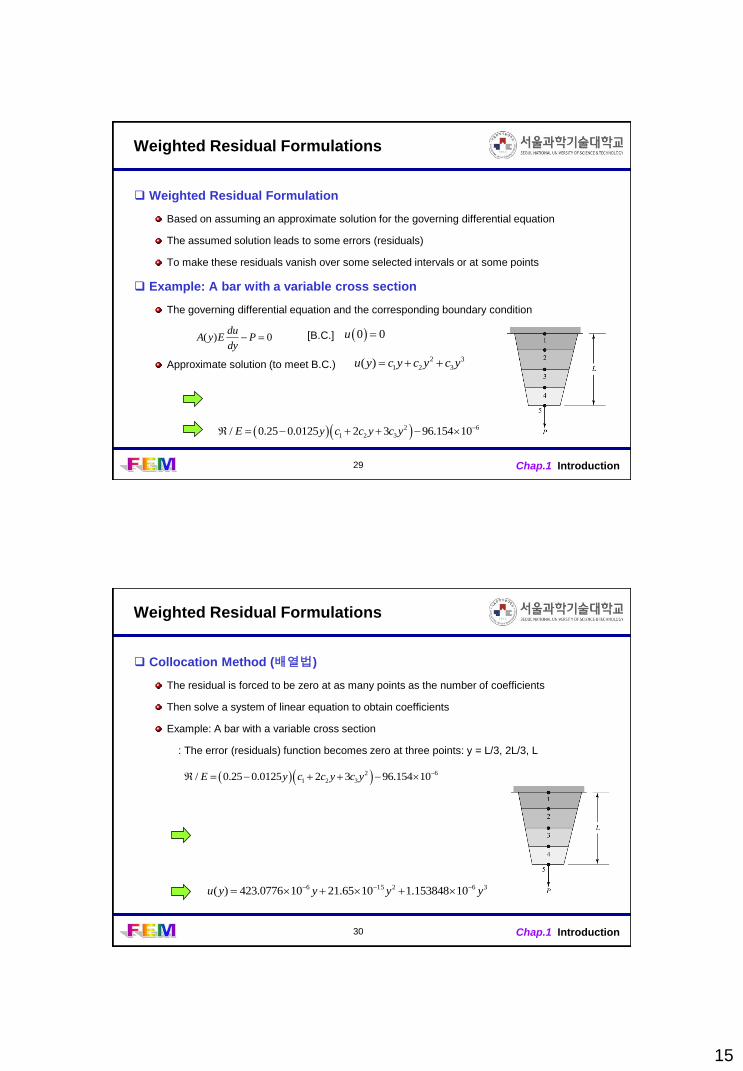
Weighted Residual Formulation
Based on assuming an approximate solution for the governing differential equation
The assumed solution leads to some errors (residuals)
To make these residuals vanish over some selected intervals or at some points
Example: A bar with a variable cross section
The governing differential equation and the corresponding boundary condition
Approximate solution (to meet B.C.)
( ) 0du
A y E Pdy
[B.C.] 0 0u
2 3
1 2 3( )u y c y c y c y
2 6
1 2 3/ 0.25 0.0125 2 3 96.154 10E y c c y c y
30 Chap.1 Introduction
Weighted Residual Formulations
Collocation Method (배열법)
The residual is forced to be zero at as many points as the number of coefficients
Then solve a system of linear equation to obtain coefficients
Example: A bar with a variable cross section
: The error (residuals) function becomes zero at three points: y = L/3, 2L/3, L
362156 10153848.11065.21100776.423)( yyyyu
2 6
1 2 3/ 0.25 0.0125 2 3 96.154 10E y c c y c y
16
31 Chap.1 Introduction
Weighted Residual Formulations
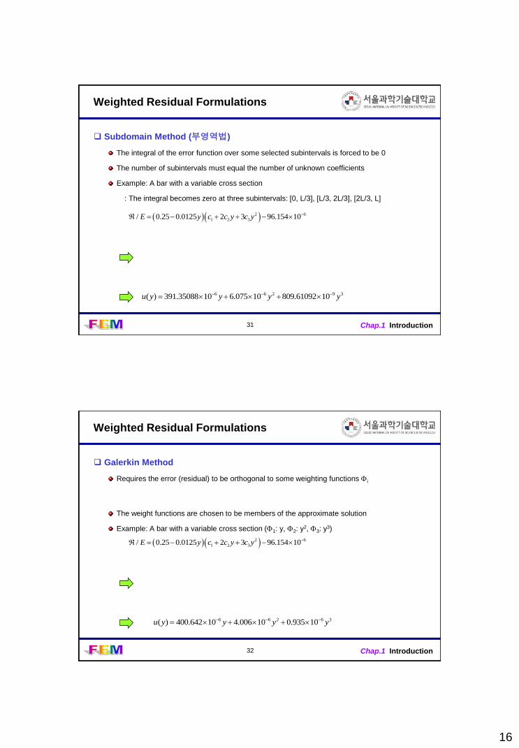
Subdomain Method (부영역법)
The integral of the error function over some selected subintervals is forced to be 0
The number of subintervals must equal the number of unknown coefficients
Example: A bar with a variable cross section
: The integral becomes zero at three subintervals: [0, L/3], [L/3, 2L/3], [2L/3, L]
39266 1061092.80910075.61035088.391)( yyyyu
2 6
1 2 3/ 0.25 0.0125 2 3 96.154 10E y c c y c y
32 Chap.1 Introduction
Weighted Residual Formulations
Galerkin Method
Requires the error (residual) to be orthogonal to some weighting functions i
The weight functions are chosen to be members of the approximate solution
Example: A bar with a variable cross section (1: y, 2: y2, 3: y
3)
36266 10935.010006.410642.400)( yyyyu
2 6
1 2 3/ 0.25 0.0125 2 3 96.154 10E y c c y c y
17
33 Chap.1 Introduction
Weighted Residual Formulations
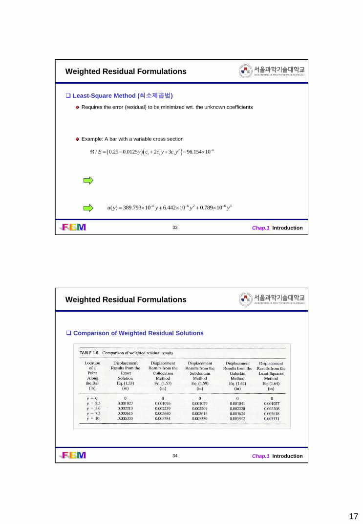
Least-Square Method (최소제곱법)
Requires the error (residual) to be minimized wrt. the unknown coefficients
Example: A bar with a variable cross section
36266 10789.010442.610793.389)( yyyyu
2 6
1 2 3/ 0.25 0.0125 2 3 96.154 10E y c c y c y
34 Chap.1 Introduction
Weighted Residual Formulations
Comparison of Weighted Residual Solutions