Embed Size (px)
Citation preview

Chapter 1 Spectral method in Matlab Centered second-order and 4-th order finite difference on uniform grid
(Eq. 1) ( ) ( ) ( )2
1 1 3
2 3!j j
j
u udu hx u cdx h
+ −−= −
(Eq. 2) ( ) ( ) ( )4
2 1 1 2 58 812 30
j j j jj
u u u udu hx u cdx h
+ + − −− + − += +
We can use another representation to derive this formula, consider polynomial interpolation
( )jp x with degree for smooth over 2≤ u 1 1,j jx x− +⎡ ⎤⎣ ⎦ .
( ) ( ) ( ) ( )1 1 0 1 1j j j jp x u a x u a x u a x− − += + +
satisfying ( )1 1j j jp x u− −= , and ( )j jp x u= j ( )1j j jp x u 1+ += . In other words,
are Lagrange polynomial satisfying ( ) ( ) ( )1 0 1, ,a x a x a x−
(Eq. 3)
( )( )( )
1 1
1
1 1
1
0
0
j
j
j
a x
a x
a x
− −
−
− +
⎧ =⎪⎪ =⎨⎪
=⎪⎩
,
( )( )( )
0 1
0
0 1
0
1
0
j
j
j
a x
a x
a x
−
+
⎧ =⎪⎪ =⎨⎪
=⎪⎩
and
( )( )( )
1 1
1
1 1
0
0
1
j
j
j
a x
a x
a x
−
+
⎧ =⎪⎪ =⎨⎪
=⎪⎩
we know
( ) ( )( )( )( )
( )( )1 11 2
1 1 1 2j j j j
j j j j
x x x x x x x xa x
hx x x x+ +
−− − +
− − − −= =
− −, ( )1
12ja xh−−
=
( ) ( )( )( )( )
( )( )1 1 1 10 2
1 1
j j j j
j j j j
x x x x x x x xa x
hx x x x− + − +
− +
− − − −= =
−− −, ( )0 0ja x =
( ) ( )( )( )( )
( )( )1 11 2
1 1 1 2j j j j
j j j j
x x x x x x x xa x
hx x x x− −
+ − +
− − − −= =
− −( )1
12ja xh
= ,
( ) ( ) ( ) ( ) 1 11 1 0 1 1|
2j
j jj x x j j j j j j
u ud p x u a x u a x u a xdx h
+ −= − − +
−= + + =
If we write 1
2j j
j
u uw
h+ −
= 1− or 2 1 18 812
j j j jj
u u u uw
h2+ + − −− + − +
= , then general matrix form can
be represented as , see Figure 1 and Figure 2. In fact matrix w Au= A is skew symmetry, say
, this can be obtained from antiHermitian of operator TA A= −ddx
under periodic boundary
1
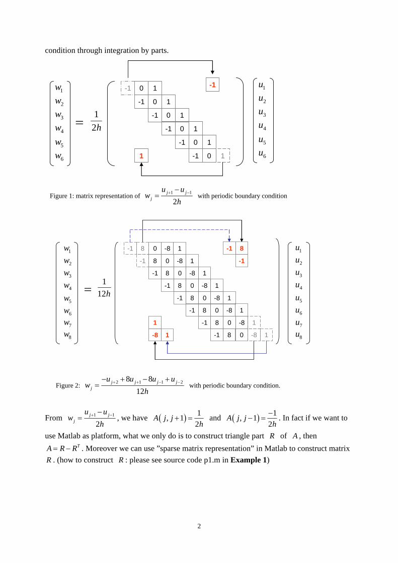
condition through integration by parts.
-1 0 1
-1 0 1
-1 0 1
-1 0 1
-1 0 1
-1 0 1
1w
2w
3w
4w
5w
6w
-1
1
1u
2u
3u
4u
5u
6u
=1
2h
Figure 1: matrix representation of 1 1
2j j
j
u uw
h+ −−
= with periodic boundary condition
-1 8 0 -8 1
-1 8 0 -8 1
-1 8 0 -8 1
-1 8 0 -8 1
-1 8 0 -8 1
-1 8 0 -8 1
-1 8 0 -8 1
1w
2w
3w
4w
5w
6w
=1
12h
-1 8 0 -8 17w8w
1u
2u
3u
4u
5u
6u
7u8u
-1 8
-1
-8 1
1
Figure 2: 2 1 18 812
j j j jj
u u u uw
h+ + −− + − +
= 2− with periodic boundary condition.
From 1 1
2j j
j
u uw
h+ −−
= , we have ( ) 1, 12
A j jh
+ = and ( ) 1, 12
A j jh−
− = . In fact if we want to
y do is to construc gle part use Matlab as platform, what we onl t trian R of A , then TA R R= − . Moreover we can use ”sparse matrix representation” in Matlab to construct matrix
R . (how to construct R : please see source code p1.m in Example 1)
2
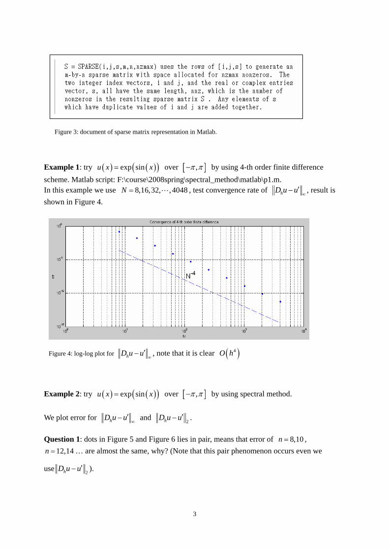
Figure 3: document of sparse matrix representation in Matlab.
Example 1: try over ( ) ( )(exp sinu x x= ) [ ],π π− by using 4-th order finite difference scheme. Matlab script: F:\course\2008spring\spectral_method\matlab\p1.m. In this example we use , test convergence rate of 8,16,32, , 4048N = hD u u
∞′− , result is
shown in Figure 4.
Figure 4: log-log plot for hD u u∞′− , note that it is clear ( )4O h
Example 2: try over ( ) ( )(exp sinu x x= ) [ ],π π− by using spectral method.
We plot error for hD u u∞′− and
2hD u u′− .
Question 1: dots in Figure 5 and Figure 6 lies in pair, means that error of , … are almost the same, why? (Note that this pair phenomenon occurs even we
use
8,10n =12,14n =
2hD u u′− ).
3

Figure 5: ”spectral accuracy” of the spectral method, it achieve machine accuracy. Sup-norm
Figure 6: ”spectral accuracy” of the spectral method, it achieve machine accuracy. 2-norm
Table 1: we list the value of pair ( 2L err− )
4,6n = 8,10n = 12,14n = 2L err− 0.24777190419502
0.33078448076569 0.00871672632422 0.00864342870238
0.94197188122419E-4 0.84097522689018E-4
16,18n = 20, 22n = 24, 26n =
2L err− 0.50008967910710E-6 0.42247516569957E-6
0.15812146492563E-8 0.12910423145203E-8
0.33254794093191E-110.26512109052603E-11
4

Table 2: we list the value of pair ( L err∞ − )
4,6n = 8,10n = 12,14n =
L err∞ − 0.17520119364380 0.16307358056713
0.00431791109859 0.00316947217836
0.38249095565268E-4 0.25253568612049E-4
16,18n = 20, 22n = 24, 26n =
L err∞ − 0.17618931913432E-6 0.10953028789507E-6
0.49879544938847E-9 0.29827984526776E-9
0.97200025805932E-12 0.59258153939368E-12
Table 3: we list the value of pair ( L err∞ − ) for arprec 128 digits
28,30n = 1.32624221983015620680098434362948e-15 7.56612859983412967818296086049246e-16
32,34n = 1.39095872807168126193852953110517e-18 7.81451569905447385343012380339833e-19
36,38n = 1.14244909925972473070099230882981e-21 6.34086538799698880852642854985210e-22
40, 42n = 7.54806757417172375166373940244838e-25 4.14826359601086676154821757222175e-25
44, 46n = 4.09864701833461299055736676547760e-28 2.23423056735975763167625559605640e-28
48,50n = 1.86164252456817011022120353206289e-31 1.00786673375963438339376505661880e-31
52,54n = 7.17767982003012719000648270914229e-35 3.86321334725399173651104700894601e-35
56,58n = 2.37854454643974045195143562239834e-38 1.27374376983182194482918312198058e-38
60,62n = 6.84730032444346812021198287838704e-42 3.65071328394049314224342346654448e-42
64,66n = 1.72836808647069444865147310660496e-45 9.17936617551766050908476538695563e-46
68,70n = 3.85647559072931642402400673411656e-49 2.04115689771413325003291669779317e-49
72,74n = 7.66124774385363632507038345929950e-53 4.04254667547222108076077515483580e-53
76,78n = 1.36375587422112860698500475832273e-56 7.17625294246753762277314925189095e-57
80,82n = 2.18769132299786362708446911624823e-60 1.14833541792638712588483843196297e-60
84,86n = 3.17896250168716103543670487976991e-64 1.66490575382791587484894062926081e-64
88,90n = 4.20398304881730575304253164828023e-68 2.19721922822932053740570006526006e-68
92,94n = 5.08108143833400125413169287191248e-72 2.65065013672443604039455837009901e-72
96,98n = 5.63449984243390032676388653577986e-76 2.93428197672848600468452855610906e-76
5

Table 4: we compute Fourier component for 1
ˆ jN
ikxk j
jv h e v−
=
= ∑ 0,1, 2, ,k m= ,
since . Since , we represent it as two value, real part (top value) and imaginary part (bottom value)
2N m=
ˆ ˆ ˆk k Nv v v∗− −= = k ˆkv C∈
8n = 10n = 12n = 14n =
0̂V 7.95492777270178
0
7.95492651755339
0
7.95492652101937
0
7.95492652101284
0
1̂V 0
-3.55100946128190
0
-3.55099934367285
0
-3.55099937850296
0
-3.55099937842424
2̂V -0.85306906632123
0
-0.85292713831639
0
-0.85292776589386
0
-0.85292776416086
0
3̂V 0
0.14099397515943
0
0.13927827358326
0
0.13928835644092
0
0.13928832168940
4̂V 0.03439566712026
0
0.01705653312949
0
0.01719845940133
0
0.01719783182714
0
5̂V eps
eps
0
-0.00171570149744
0
-0.00170561863991
6̂V -0.00028260085474
0
-0.00014067458291
0
7̂V eps
eps
16n = 18n = 20n = 22n =
0̂V 7.95492652101284
0
7.95492652101284
0
7.95492652101284 7.95492652101285
1̂V 0
-3.55099937842436
0
-3.55099937842436
0
-3.55099937842436
0
- 3.55099937842436
2̂V -0.85292776416412
0
-0.85292776416412
0
-0.85292776416412
0
-0.85292776416412
0
3̂V 0
0.13928832176800
0
0.13928832176787
0
0.13928832176788
0
0.13928832176788
4̂V 0.01719783356013
0
0.01719783355686
0
0.01719783355687
0
0.01719783355687
0
5̂V 0
-0.00170565339142
0
-0.00170565331282
0
-0.00170565331295
0
- 0.00170565331295
6̂V -0.00014130215710
0
-0.00014130042411
0
-0.00014130042738
0
-0.00014130042737
0
6
7̂V 0
0.00001008285753
0
0.00001004810602
0
0.00001004818462
0
0.00001004818449
8̂V 0.00000125168893
0
0.00000062411474
0
0.00000062584773
0
0.00000062584446
0
9̂V Eps
Eps
0
- 0.00000003475152
0
-0.00000003467292
10V̂ -0.00000000345946
0
-0.00000000172646
0
11V̂ Eps
Eps
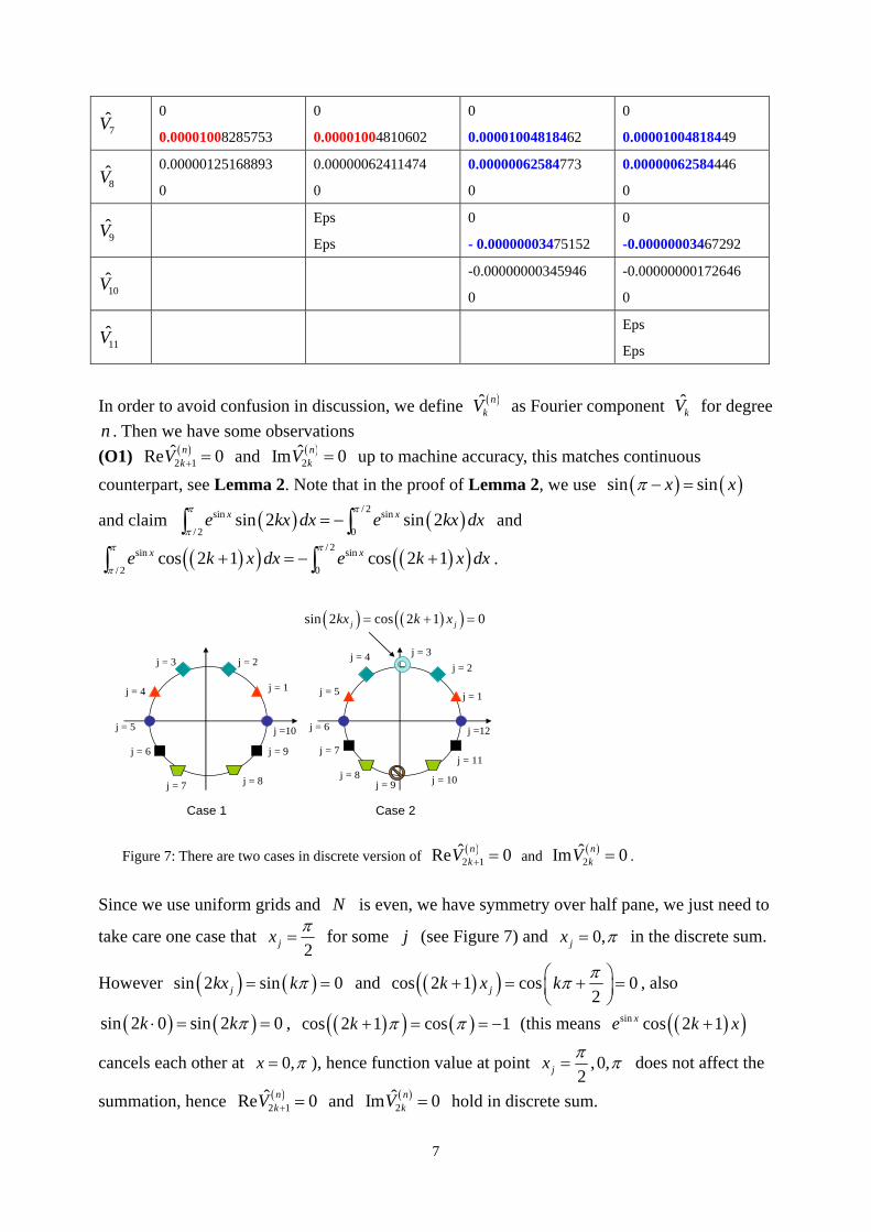
In order to avoid confusion in discussion, we define ( )ˆ n
kV as Fourier component for degree . Then we have some observations
k̂Vn(O1) ( )
2 1ˆRe 0n
kV + = and ( )2̂Im 0n
kV = up to machine accuracy, this matches continuous counterpart, see Lemma 2. Note that in the proof of Lemma 2, we use ( ) ( )sin sinx xπ − =
and claim and
.
( ) ( )/ 2sin sin
/ 2 0sin 2 sin 2x xe kx dx e kx
π π
π= −∫ ∫ dx
dx( )( ) ( )( )/ 2sin sin
/ 2 0cos 2 1 cos 2 1x xe k x dx e k x
π π
π+ = − +∫ ∫
j =10
j = 1
j = 2j = 3
j = 4
j = 5
j = 6
j = 7 j = 8
j = 9
j =12
j = 1
j = 2j = 4
j = 5
j = 6
j = 7
j = 8 j = 10
j = 11
j = 3
j = 9
( ) ( )( )sin 2 cos 2 1 0j jkx k x= + =
Case 1 Case 2
Figure 7: There are two cases in discrete version of ( )2 1ˆRe 0n
kV + = and ( )2̂Im 0n
kV = .
Since we use uniform grids and is even, we have symmetry over half pane, we just need to
take care one case that
N
2jx π= for some (see Figure 7) and j 0,jx π= in the discrete sum.
However and ( ) ( )sin 2 sin 0jkx kπ= = ( )( )cos 2 1 cos 02jk x k ππ⎛ ⎞+ = +⎜ ⎟
⎝ ⎠= , also
, ( ) ( )sin 2 0 sin 2 0k kπ⋅ = = ( )( ) ( )cos 2 1 cos 1k π π+ = = − x+ (this means e k
cancels each other at
( )( )sin cos 2 1x
0,x π= ), hence function value at point ,0,2jx π π= does not affect the
summation, hence ( )2 1ˆRe 0n
kV + = and ( )2̂Im 0n
kV = hold in discrete sum.
7
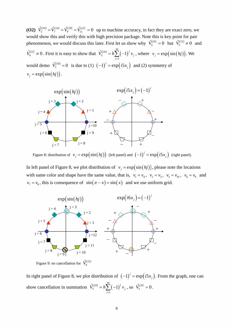
(O2) ( ) ( ) ( ) ( )10 14 18 225 7 9 11ˆ ˆ ˆ ˆ 0V V V V= = = = up to machine accuracy, in fact they are exact zero, we
would show this and verify this with high precision package. Note this is key point for pair phenomenon, we would discuss this later. First let us show why ( )10
5̂ 0V = but ( )125̂ 0V ≠ and
( )126̂ 0V ≠ . First it is easy to show that ( ) ( )
1010
51
ˆ 1 jj
jV h
=
= −∑ v , where ( )( )exp sinjv h= j . We
would demo ( )105̂ 0V = is due to (1) ( ) ( )1 exp 5j
ji x− = and (2) symmetry of
( )( )exp sinjv h= j .
( )( )exp sin hj ( ) ( )exp 5 1 jji x = −
+
+
+
+
+
−
−
−
−
−
j =10
j = 1
j = 2j = 3
j = 4
j = 5
j = 6
j = 7 j = 8
j = 9
Figure 8: distribution of ( )(exp sinjv = )hj (left panel) and ( ) ( )1 exp 5jji x− = (right panel).
In left panel of Figure 8, we plot distribution of ( )( )exp sinjv = hj , please note the locations
with same color and shape have the same value, that is, 1 4v v= , 2 3v v= , , and , this is consequence of
5 1v v= 0 9
8
6v v=
7v v= ( ) ( )sin sinx xπ − = and we use uniform grid.
( )( )exp sin hj ( ) ( )exp 6 1 jji x = −
+−
+
++
+
+
−
−
−
−−
j =12
j = 1
j = 2j = 4
j = 5
j = 6
j = 7
j = 8 j = 10
j = 11
j = 3
j = 9
Figure 9: no cancellation for ( )126̂V
In right panel of Figure 8, we plot distribution of ( ) ( )1 exp 5jji x− = . From the graph, one can
show cancellation in summation ( ) ( )10
105
1
ˆ 1 jj
jV h
=
= −∑ v , so ( )105̂ 0V = .
8

However when , 12n = ( ) ( ) 51 exp 5 exp12
jji x i j⎛− ≠ = ⎜
⎝ ⎠⎞⎟ , hence no cancellation occurs, that is
( )125̂ 0V ≠ . Moreover ( )12
6̂ 0V ≠ is result of no cancellation, see Figure 9.
similarly, ( ) ( ) ( )14 18 227 9 11ˆ ˆ ˆ 0V V V= = = .
Remark 1: From above argument, (O2) is valid when ( ) ( )V x V xπ= − , for example,
on [( )( )sinV V x= ]0, 2π . However ( )cos x is not permitted though ( ) 2cos 1 sinx x= − ,
why? Since in general ( ) 2cos 1 sinx x= ± − , the sign depends on branch, that is
( ) (cos cos )x xπ − ≠ .
(O3) ( ) ( )8 10
4 4ˆ ˆ2V V≈ , ( ) ( )12 14
6 6ˆ ˆ2V V≈ , ( ) ( )16 18
8̂ˆ2V V≈ 8 and ( ) ( )20 22
10 10ˆ ˆ2V V≈ , although we cannot
interpret this phenomenon, but such fact is also a key to pair phenomenon. Now we explain this.
First, in chapter 3 (see chap3.doc), we split ( )ˆ NmV into 2 parts, (say ( ) ( ) ( )1ˆ ˆ ˆ
2N Nm m mV V V− = ← N ), for
symmetry inteepolant ( )p x defined by
(Eq. 4) ( ) ( )1 ˆ2
mNikx
N kk m
p x e Vπ =−
= Ρ ∑ for [ ]0,2x π∈ , 2N m=
where (principal value) indicates that the terms Ρ k m= ± are multiplied by 12
.
Hence ( )84
1 ˆ 0.017197833560132
V = and then ( ) ( )8 104 4
1 ˆ ˆ 1.413004306399998e-0042
V V− = .
Now we estimate the difference between ( )8p x and ( )10p x .
( ) ( ) ( ) ( )( ) ( ) ( ) ( )3
10 8 10 8 1010 8
3 4
1 1 1 1ˆ ˆ ˆ ˆ ˆ2 2 2 2
ikx ikx ikxk k k k k
k k
p x p x e V V e V V e Vπ π π=− =± =±
⎛ ⎞− = − + − +⎜ ⎟⎝ ⎠
∑ ∑5k
∑
However we have shown ( )105̂ 0V = , so
( ) ( ) ( ) ( ) ( ) ( )3
10 8 10 810 8
3 4
1 1ˆ ˆ ˆ ˆ2 2k k k k
k k
p x p x V V V Vπ π=− =±
− ≤ − + −∑ ∑ 12
( ) ( )10 80 0ˆ ˆ 1.255148390555405e-006V V− = ( ) ( )10 8
1 1ˆ ˆ 1.011760904967574e-005V V− = ( ) ( )10 8
2 2ˆ ˆ 1.419280048400307e-004V V− = ( ) ( )10 8
3 3ˆ ˆ 0.00171570157617V V− =
( ) ( )8 104 4
1 ˆ ˆ 1.413004306399998e-0042
V V− =
Hence ( ) ( )10 8 6.396994825534096e-004p x p x− ≤ for any [ ]0,2x π∈ .
Further ( ) ( ) ( ) ( )( ) ( ) ( )3
10 8 10 810 8
3 4
1 1ˆ ˆ ˆ ˆ2 2
ikx ikxk k k k
k k
p x p x ike V V ike V Vπ π=− =±
⎛ ⎞′ ′− = − + −⎜ ⎟⎝ ⎠
∑ ∑ 12
( ) ( )10 8 0.00191185832541p x p x′ ′− ≤ for any [ ]0,2x π∈ .
9

This number is about 8 ,
12 I
p V∞
′ ′− , hence pair phenomenon occurs at . 8,10n =
Table 5: we copy data from Table 2 and add two new fields, one is 2n nerr err +− and the other
is ( ) ( )2n np x p x+′ ′− , 2n nerr err +− is difference of two value in the field L err∞ − , it measure derivation between pair, for example
8 10 0.00431791109859 0.00316947217836 0.00114843892023err err− = − =
( ) ( )2n np x p x+′ ′− measure derivation due to ( ) ( )2ˆ ˆn nk kV V +− .
8,10n = 12,14n =
L err∞ − 0.00431791109859 0.00316947217836
0.38249095565268E-4 0.25253568612049E-4
2n nerr err +− 0.00114843892023 1.299552695321900e-5
( ) ( )2n np x p x+′ ′− 0.00191185832541 1.807600691270616e-5
16,18n = 20, 22n = 24, 26n =
L err∞ − 0.17618931913432E-6
0.10953028789507E-6
0.49879544938847E-9
0.29827984526776E-9
0.97200025805932E-12
0.59258153939368E-12
2n nerr err +− 6.665903123925001e-8 2.00515604120710e-10 3.794187186656399e-13
( ) ( )2n np x p x+′ ′−
8.527607765287214e-8 2.441827585710109e-10 5.089522571307543e-13
From above data, we would find ( ) ( )2n n n nerr err p x p x+ ′ ′− ≈ − 2+ , this proves our idea that pair phenomenon occurs due to 3 reasons (1) ( )
2 1ˆRe 0n
kV + = and ( )2̂Im 0n
kV =
(2) ( ) ( ) ( ) ( )10 14 18 225 7 9 11ˆ ˆ ˆ ˆ 0V V V V= = = =
(3) ( ) ( )8 104 4ˆ ˆ2V V≈ (, ) ( )12 14
6 6ˆ ˆ2V V≈ , ( ) ( )16 18
8 8ˆ ˆ2V V≈ and ( ) ( )20 22
10 10ˆ ˆ2V V≈
(4) From chap3.doc, we have shown
Lemma 1: 1
ˆ ˆˆ 2k k k Npp
v V V∞
+=
− ≤ ∑ for 0,1, 2, , 1k N= −
Moreover from experimental result for ( )( )exp sinV = x (see below), we found that 1k̂ kV
k∼ ,
hence the error between discrete Fourier component ( ) ( )2ˆ ˆn nk kv v +− for 0,1, 2, , / 2k n= can
be neglected. 10
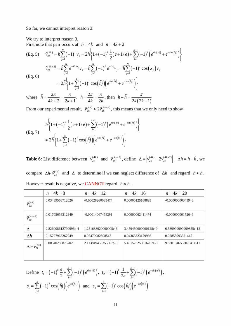
So far, we cannot interpret reason 3. We try to interpret reason 3. First note that pair occurs at and 4n = k 4 2n k= +
(Eq. 5) ( ) ( ) ( ) ( ) ( ) ( ) ( )( )1
4 sin sin2
1 1
1ˆ 1 2 1 1 1/ 12
N kj k jk hj hj
k jj j
v h v h e e e e−
−
= =
⎧ ⎫= − = + − + + − +⎨ ⎬
⎩ ⎭∑ ∑
(Eq. 6)
( ) ( ) ( ) ( )
( ) ( ) ( ) ( )( )
24 22
1 1 1
sin sin
1
ˆ 1 1 co
2 1 1 cos
j jN N N
j ji kx ixkk j j
j j j
kj hj hj
j
v h e v h e v h x
h hj e e
− −+
= = =
−
=
= = − = −
⎧ ⎫= + − +⎨ ⎬
⎩ ⎭
∑ ∑ ∑
∑
s j jv
where 24 2 2
hk k 1π π
= =+ +
, 24 2
hk kπ π
= = , then ( )2 2 1
h hk k
π− =
+
From our experimental result, ( ) ( )4 42 2ˆ ˆ2k k
k kv v 2+≈ , this means that we only need to show
(Eq. 7) ( ) ( ) ( ) ( ) ( )( )
( ) ( ) ( ) ( )( )
1sin sin
1
sin sin
1
11 1 1/ 12
2 1 1 cos
kk j hj hj
j
kj hj hj
j
h e e e e
h hj e e
−−
=
−
=
⎧ ⎫+ − + + − +⎨ ⎬
⎩ ⎭⎧ ⎫
≈ + − +⎨ ⎬⎩ ⎭
∑
∑
Table 6: List difference between and ( )42ˆ
kkv ( )4 2
2ˆk
kv + , define ( ) ( )4 4 22 2ˆ ˆ2k k
k kv v +∆ = − h h h∆ = −, , we
compare and to determine if we can neglect difference of ( )42ˆ
kkh v∆ ⋅ ∆ h∆ and regard h h≈ .
However result is negative, we CANNOT regard h h≈ .
4 8n k= = 4 1n k= = 2 6 4 1n k= = 4 2n k= = 0
( )42ˆ
kkv
0.03439566712026 -0.00028260085474
0.00000125168893
-0.00000000345946
( )4 22ˆ
kkv +
0.01705653312949 -0.00014067458291
0.00000062411474
-0.00000000172646
∆ 2.826008612799996e-4 1.251688920000005e-6 3.459450000000128e-9 6.539999999999855e-12
h∆ 0.15707963267949 0.07479982508547 0.04363323129986 0.02855993321445
( )4ˆ kh v∆ ⋅ 2k
0.00540285875702 2.113849450355667e-5 5.461523259816207e-8 9.880194655807041e-11
Define ( ) ( ) ( )( )1
sin1
11 1
2
kk j hj
j
et e−
=
= − + −∑ , ( ) ( ) ( )( )1
sin2
1
11 12
kk j hj
jt e
e
−−
=
= − + −∑ ,
and ( ) ( ) ( )( )sin1
11 cos
kj hj
js hj
=
= −∑ e ( ) ( ) ( )( )sin2
11 cos
kj hj
js hj −
=
= −∑ e
11

( )1 1 1 22h t s t s∆ = − + − 2 and ( )( ) ( )4 22 1 2
1 ˆ2 12
kkh h s s v
k 2+∆ = − + + =
Then ( ) ( )42 1 2ˆ 2 1k
kv h t t= + + (, ) ( )4 22 1 2ˆ 2 1k
kv h s s+ = + + and then ( ) ( )4 4 22 2 1ˆ ˆk k
k kv v +− = ∆ + 2∆
2 6
4 8n k= = 4 1n k= = 4 1n k= = 4 2n k= = 0
( )4 22ˆ
kkv +
0.01705653312949 -1.4067458291e-4 6.2411474e-7 -1.72646e-9
∆ 2.826008612799996e-4 1.251688920000005e-6 3.459450000000128e-9 6.539999999999855e-12
1t -0.66897406741795 -0.63041950969349 -0.59800207628710 -0.57848539389295
2t -0.30912897080952 -0.36985035424424 -0.40199633001306 -0.42151461161294
1s -0.65635567309515 -0.61768932891181 -0.58985808333448 -0.57283605860995
2s -0.33007116910701 -0.38246739447485 -0.41014102268702 -0.42716394441257
1ht -0.52541100391058 -0.33008688338879 -0.23483486621187 -0.18173654636631
2ht -0.24278932592674 -0.19365319263688 -0.15786358964238 -0.13242272072240
1hs -0.41240043214754 -0.27721832255859 -0.20589931347379 -0.16360159576731
2hs -0.20738983200567 -0.17165096524569 -0.14316622486770 -0.12199773724045
1∆ 0.01307500070840 -1.184805080196554e-4 5.495598519973221e-7 -1.560346593471024e-9
2∆ 0.00426413328237 -2.344576381762684e-5 7.801434217854332e-8 -1.726463642529372e-10
Because 2 2
hhk π= − , we can rewrite and as 1s 2s
( ) ( ) ( )( ) ( ) ( ) ( )1sin cos / 2
11
1 cos 1 sin / 2k
j khj h
js hj e h
−
=
= − + −∑ e
e
and
( ) ( ) ( )( ) ( ) ( ) ( )1sin cos / 2
21
1 cos 1 sin / 2k
j khj h
js hj e h
−− −
=
= − + −∑
( ) ( )( ) ( ) ( )( ) ( ) ( ) ( )1sin cos / 2sin
1 11
1 cos 1 in / 22
kj khj hhj
j
et s e hj e s h e−
=
⎡ ⎤⎡ ⎤− = − − + − −⎢ ⎥⎢ ⎥⎣ ⎦ ⎣ ⎦∑
( ) ( )( ) ( ) ( )( ) ( ) ( ) ( )1sin cos / 2sin
2 21
11 cos 1 sin / 22
kj khj hhj
jt s e hj e h e
e
−− −−
=
⎡ ⎤⎡ ⎤− = − − + − −⎢ ⎥⎢ ⎥⎣ ⎦ ⎣ ⎦∑
Then if we want to show ( ) ( )4 42 2ˆ ˆ2k k
k kv v 2+≈ , it suffices to show ( )4 21 2
1 ˆ12
kkv
k+⎛ ⎞∆ ≈ −⎜ ⎟
⎝ ⎠.
Another view: if we divide 1 112 2
= + , then we may regard summation in as sum of
Trapezoid rule, so is
( )42ˆ
kkv
( )4 22ˆ
kkv + , then we rewrite them as
( ) ( ) ( ) ( )( ) ( ) ( ) ( )( )1 1
4 sin sin sin2
0 0
ˆ 1 1k k
j jk hj hj h hjk
j jv h e e h e e
− −+ − −
= =
= − − + − −∑ ∑ sin hj h+
12
Possible solution ( ) ( ) ( ) ( )sin sin sincos
xx y t
ye e t e= + ∫ dt
dt
sin t dt
Then . ( ) ( ) ( ) ( )sin sin sincoshj hhj hj h t
hje e h t e
++− = − ∫( ) ( ) ( ) ( ) ( ) ( ) ( )
1 14 sin
20 0
ˆ 1 cos 1 cosk khj h hj hj jk t
k hj hjj j
v h t e dt h t e− −+ + −
= =
= − − + −∑ ∑∫ ∫
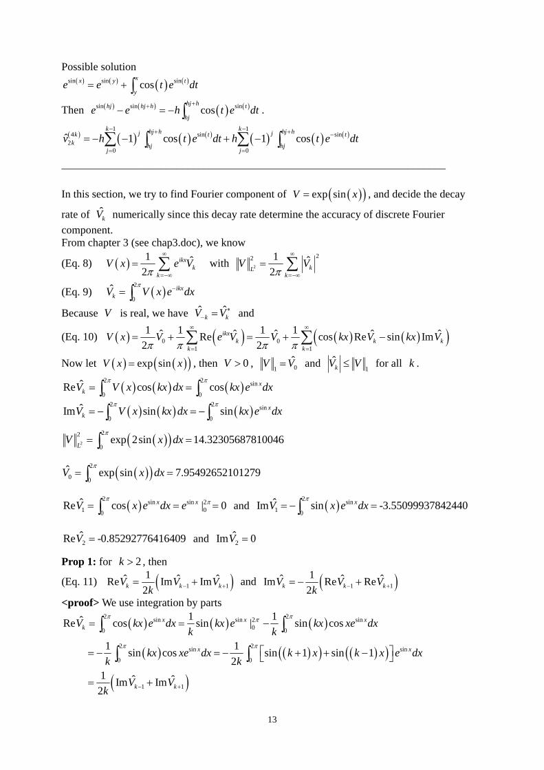
______________________________________________________________________ In this section, we try to find Fourier component of ( )( )exp sinV = x , and decide the decay
rate of numerically since this decay rate determine the accuracy of discrete Fourier component.
k̂V
From chapter 3 (see chap3.doc), we know
(Eq. 8) ( ) 1 ˆ2
ikxk
kV x e V
π
∞
=−∞
= ∑ with 2
22 1 ˆ2 kL
kV V
π
∞
=−∞
= ∑
(Eq. 9) ( )2
0ˆ ikxkV V x e
π −= ∫ dx
Because is real, we have V ˆ ˆk kV V ∗
− = and
(Eq. 10) ( ) ( ) ( ) ( )( )0 01 1
1 1 1 1ˆ ˆ ˆ ˆRe cos Re sin Im2 2
ikxk k
k k
V x V e V V kx V kx Vπ π π π
∞ ∞
= =
= + = + −∑ ∑ k̂
Now let ( ) ( )( )exp sinV x x= , then , 0V > 01ˆV V= and
1k̂V V≤ for all . k
( ) ( ) ( )2 2 sin
0 0ˆRe cos cos xkV V x kx dx kx e
π π= =∫ ∫ dx
dx
( ) ( ) ( )2 2 sin
0 0ˆIm sin sin xkV V x kx dx kx e
π π= − = −∫ ∫
( )( )2
22
0exp 2sin 14.32305687810046
LV x dx
π= =∫
( )( )2
0 0ˆ exp sin 7.95492652101279V x dx
π= =∫
( )2 sin sin 2
1 00ˆRe cos | 0x xV x e dx e
π π= = =∫ ( )2 sin
1 0ˆIm sin -3.55099937842440xV x e dx
π= − =∫ and
2̂Re -0.85292776416409V = and 2̂Im 0V =
Prop 1: for , then 2k >
(Eq. 11) ( )1 11ˆ ˆRe Im Im
2k kV Vk −= + k̂V + and ( )1 1
1ˆ ˆIm Re Re2k kV Vk − += − + k̂V
<proof> We use integration by parts
( ) ( ) ( )
( ) ( )( ) ( )( )
( )
2 2sin sin 2 sin00 0
2 2sin sin
0 0
1 1
1 1ˆRe cos sin | sin cos
1 1 sin cos sin 1 sin 12
1 ˆ ˆ Im Im2
x x xk
x x
k k
V kx e dx kx e kx xe dxk k
kx xe dx k x k x e dxk k
V Vk
π ππ
π π
− +
= = −
⎡ ⎤= − = − + + −⎣ ⎦
= +
∫ ∫
∫ ∫
13
( ) ( ) ( )
( ) ( )( ) ( )( )
( )
2 2sin sin 2 sin00 0
2 2sin sin
0 0
1 1
1 1ˆIm sin cos | cos cos
1 1 cos cos cos 1 cos 12
1 ˆ ˆ Re Re2
x x xk
x x
k k
V kx e dx kx e kx xe dxk k
kx xe dx k x k x e dxk k
V Vk
π ππ
π π
− +
= − = −
⎡ ⎤= − = − + + −⎣ ⎦
= − +
∫ ∫
∫ ∫
___________________________________________________________________ We can rearrange (Eq. 11) to be
(Eq. 12) or 1 1
1 1
ˆ ˆRe Re Im2
ˆ ˆIm Im Rek k
ˆ
ˆk k k
V V Vk
V V V+ −
+ −
⎡ ⎤ ⎡ ⎤ ⎡ ⎤−= − +⎢ ⎥ ⎢ ⎥ ⎢ ⎥
⎢ ⎥ ⎢ ⎥ ⎢ ⎥⎣ ⎦ ⎣ ⎦ ⎣ ⎦
k1 1
ˆ ˆ ˆ2 1k k kk V+ −V V= − + −
Remark 2: one can derive (Eq. 12) by
( ) ( ) ( )2 2 2sin sin1 10 0 0
1 1 1ˆ ˆ ˆcos2 2
ikx ikx x ikx ix ix xk k kV V x e dx e xe dx e e e e dx V V
ik ik ikπ π π− − − −
− += = = + =∫ ∫ ∫ +
for example: ( )3 1 2
ˆ ˆ ˆ4 1 0,0.13928832176804V V V= − + − = , ( )4 2 3ˆ ˆ ˆ6 1 0.01719783355585,0V V V= − + − =
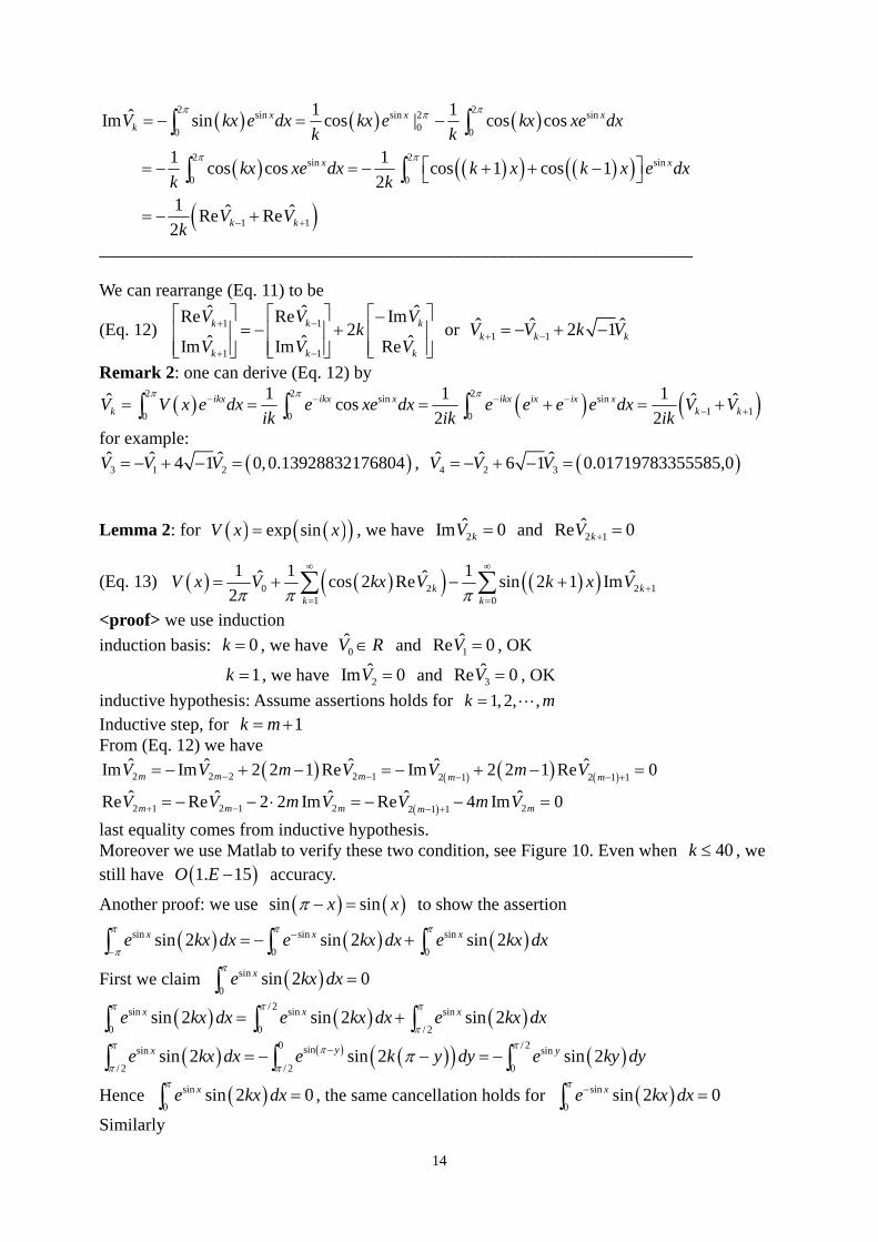
Lemma 2: for ( ) ( )(exp sinV x x= ) , we have 2̂Im 0kV = and 2 1ˆRe 0kV + =
(Eq. 13) ( ) ( )( ) ( )( )0 21 0
1 1 1ˆ ˆcos 2 Re sin 2 1 Im2 k k
k kV x V kx V k x V
π π π
∞ ∞
+= =
= + − +∑ ∑ 2 1ˆ
<proof> we use induction induction basis: , we have and 0k = 0̂V R∈ 1̂Re 0V = , OK
, we have 1k = 2̂Im 0V = and 3̂Re 0V = , OK inductive hypothesis: Assume assertions holds for 1, 2, ,k m= Inductive step, for 1k m= +From (Eq. 12) we have
( ) ( ) ( ) ( )2 2 2 2 1 2 1 2 1 1ˆ ˆ ˆ ˆ ˆIm Im 2 2 1 Re Im 2 2 1 Re 0m m m m mV V m V V m V− − − −= − + − = − + − =+
m
)
( )2 1 2 1 2 22 1 1ˆ ˆ ˆ ˆ ˆRe Re 2 2 Im Re 4 Im 0m m m mV V m V V m V+ − − += − − ⋅ = − − =
last equality comes from inductive hypothesis. Moreover we use Matlab to verify these two condition, see Figure 10. Even when , we still have accuracy.
40k ≤(1. 15O E −
Another proof: we use ( ) ( )sin sinx xπ − = to show the assertion
( ) ( ) ( )sin sin sin
0 0sin 2 sin 2 sin 2x x xe kx dx e kx dx e kx
π π π
π
−
−= − +∫ ∫ ∫ dx
dy
First we claim ( )sin
0sin 2 0xe kx dx
π=∫
( ) ( ) ( )/ 2sin sin sin
0 0 / 2sin 2 sin 2 sin 2x x xe kx dx e kx dx e kx dx
π π π
π= +∫ ∫ ∫
( ) ( ) ( )( ) ( )0 / 2sinsin sin
/ 2 / 2 0sin 2 sin 2 sin 2yx ye kx dx e k y dy e ky
π ππ
π ππ−= − − = −∫ ∫ ∫
Hence , the same cancellation holds for ( )sin
0sin 2 0xe kx dx
π=∫ ( )sin
0sin 2 0xe kx dx
π − =∫Similarly
14

( )( ) ( )( ) ( )( )sin sin sin
0 0cos 2 1 cos 2 1 cos 2 1x x xe k x dx e k x dx e k x dx
π π π
π
−
−+ = − + + +∫ ∫ ∫
we claim ( )( )sin
0cos 2 1 0xe k x dx
π+ =∫
( )( ) ( )( ) ( )( )0 / 2sin sin sin
/ 2 / 2 0cos 2 1 cos 2 1 cos 2 1x y ye k x dx e k y dy e k y
π π
π ππ+ = − − + = − +∫ ∫ ∫ dy
Figure 10: we verify condition and Re2̂Im 0kV = 2 1ˆ 0kV + = for k 1:10= by using trapezoid rule
to do integration. It is clear that all data reach machine accuracy.
________________________________________________________________________ From Lemma 2, we can simplify (Eq. 10) as
(Eq. 14) ( ) ( )( ) ( )( )( )0 21 0
1 1 1ˆ ˆcos 2 Re sin 2 1 Im2 k k
k kV x V kx V k x V
π π π
∞ ∞
+= =
= + − +∑ ∑ 2 1ˆ
1V
V
⎤⎥⎥⎦
where
(Eq. 15) ( )
( )
( )2 12 2
2 1 22 1 1
ˆˆ ˆReRe 2 1 Im2
ˆ ˆˆIm 2 ReIm
kk k
k kk
VV k
V kV
− −
+ − +
⎡ ⎤⎡ ⎤ ⎡− −⎢ ⎥= − +⎢ ⎥ ⎢⎢ ⎥⎢ ⎥ ⎢⎣ ⎦ ⎣⎣ ⎦
Moreover we can simplify (Eq. 15) further
(Eq. 16) ( )( )( )
( )
( )
2 12
2 1 2 1 1
ˆˆ Re1 2 2 1Reˆ ˆ4 1 8 2 1Im Im
kk
k k
VkVk k kV V
−
+ − +
⎡ ⎤⎡ ⎤ ⎡ ⎤− − −⎢ ⎥=⎢ ⎥ ⎢ ⎥− − + − ⎢ ⎥⎢ ⎥⎢ ⎥ ⎣ ⎦⎣ ⎦ ⎣ ⎦
2 0
3 1
ˆ ˆRe Re1 2ˆ ˆ4 9Im Im
V V
V V
⎡ ⎤ ⎡ ⎤− −⎡ ⎤=⎢ ⎥ ⎢⎢ ⎥− −⎣ ⎦⎢ ⎥ ⎢ ⎥⎣ ⎦⎣ ⎦
⎥ ,
4 2 0
5 3 1
ˆ ˆ ˆRe Re Re1 6 25 56ˆ ˆ ˆ8 49 204 457Im Im Im
V V V
V V V
⎡ ⎤ ⎡ ⎤ ⎡ ⎤− −⎡ ⎤ ⎡ ⎤= =⎢ ⎥ ⎢ ⎥ ⎢ ⎥⎢ ⎥ ⎢ ⎥− −⎣ ⎦ ⎣ ⎦⎢ ⎥ ⎢ ⎥ ⎢ ⎥⎣ ⎦⎣ ⎦ ⎣ ⎦
, ….
15
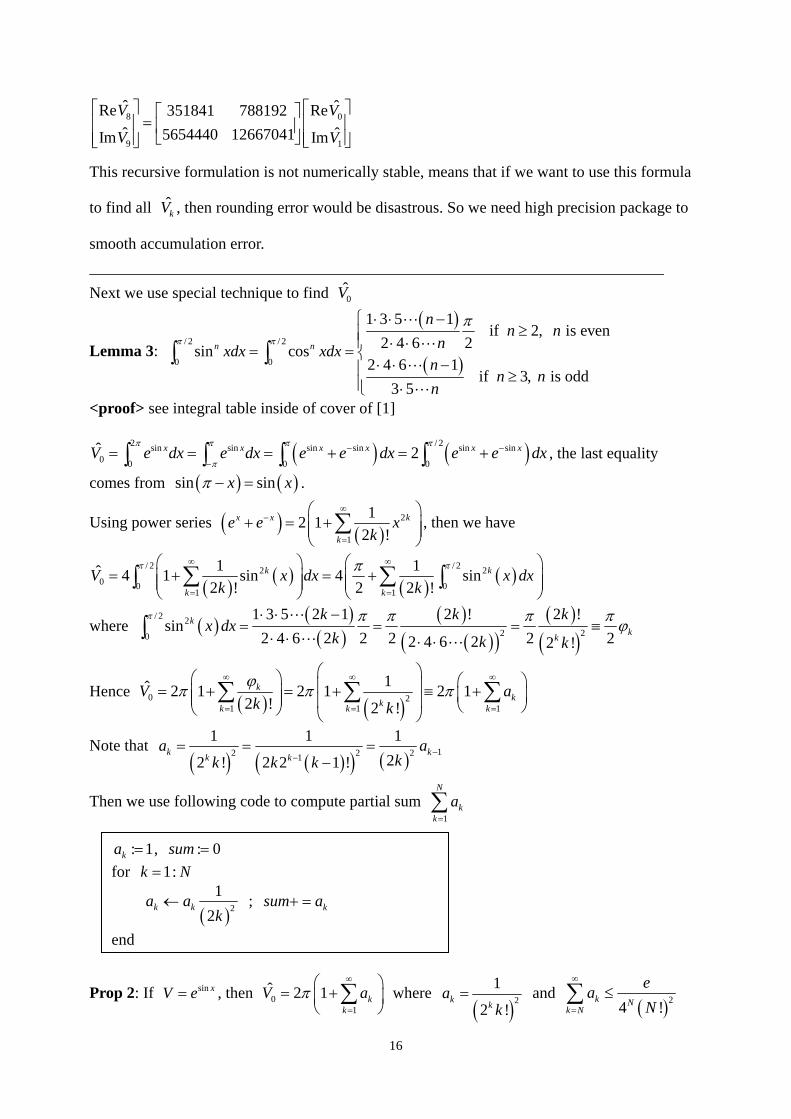
8 0
9 1
ˆ ˆRe Re351841 788192ˆ ˆ5654440 12667041Im Im
V V
V V
⎡ ⎤ ⎡ ⎤⎡ ⎤=⎢ ⎥ ⎢⎢ ⎥⎣ ⎦⎢ ⎥ ⎢ ⎥⎣ ⎦⎣ ⎦
⎥
This recursive formulation is not numerically stable, means that if we want to use this formula
to find all , then rounding error would be disastrous. So we need high precision package to
smooth accumulation error.
k̂V
________________________________________________________________________ Next we use special technique to find 0̂V
Lemma 3:
( )
( )/ 2 / 2
0 0
1 3 5 1 if 2, is even
2 4 6 2sin cos2 4 6 1
if 3, is odd3 5
n n
nn n
nxdx xdxn
n nn
π π
π⎧ ⋅ ⋅ −≥⎪⎪ ⋅ ⋅= = ⎨
⋅ ⋅ −⎪ ≥⎪ ⋅⎩
∫ ∫
<proof> see integral table inside of cover of [1]
( ) ( )2 /sin sin sin sin sin sin0 0 0 0ˆ 2x x x x xV e dx e dx e e dx e e
π π π π
π
−
−= = = + = +∫ ∫ ∫ ∫
2 x dx−
), the last equality
comes from ( ) (sin sinx xπ − = .
Using power series ( ) ( )2
1
12 12 !
x x k
ke e x
k
∞−
=
⎛ ⎞+ = +⎜⎜
⎝ ⎠∑ ⎟⎟ , then we have
( ) ( ) ( ) ( )/ 2 / 22 2
0 0 01 1
1 1ˆ 4 1 sin 4 sin2 ! 2 2 !
k k
k kV x dx
k kπ ππ∞ ∞
= =
⎛ ⎞ ⎛= + = +⎜ ⎟ ⎜⎜ ⎟ ⎜
⎝ ⎠ ⎝∑ ∑∫ ∫ x dx
⎞⎟⎟⎠
where ( ) ( )( )
( )( )( )
( )( )
/ 2 22 20
1 3 5 2 1 2 ! 2 !sin
2 4 6 2 2 2 2 22 4 6 2 2 !k
kk
k k kx dx
k k k
π π π π π ϕ⋅ ⋅ −
= = =⋅ ⋅ ⋅ ⋅
∫ ≡
Hence ( ) ( )0 2
1 1
1ˆ 2 1 2 1 2 12 ! 2 !
kkkk k
V ak k
ϕπ π π∞ ∞
= =
⎛ ⎞⎛ ⎞ ⎛ ⎞⎜ ⎟= + = + ≡ +⎜ ⎟ ⎜ ⎟⎜ ⎟ ⎜ ⎟ ⎝ ⎠⎝ ⎠ ⎝ ⎠∑ ∑
1k
∞
=∑
Note that ( ) ( )( ) ( ) 12 21
1 1 122 ! 2 2 1 !
k kk ka a
kk k k2 −
−= = =
−
Then we use following code to compute partial sum 1
N
kk
a=∑
: 1ka = , : 0sum =for 1:k N=
( )2
12
k ka ak
← ; ksum a+ =
end
Prop 2: If , then sin xV e= 01
ˆ 2 1 kk
V aπ∞
=
⎛= +⎜
⎝ ⎠
⎞⎟∑ where
( )21
2 !k k
ak
= and ( )24 !
k Nk N
eaN
∞
=
≤∑
16
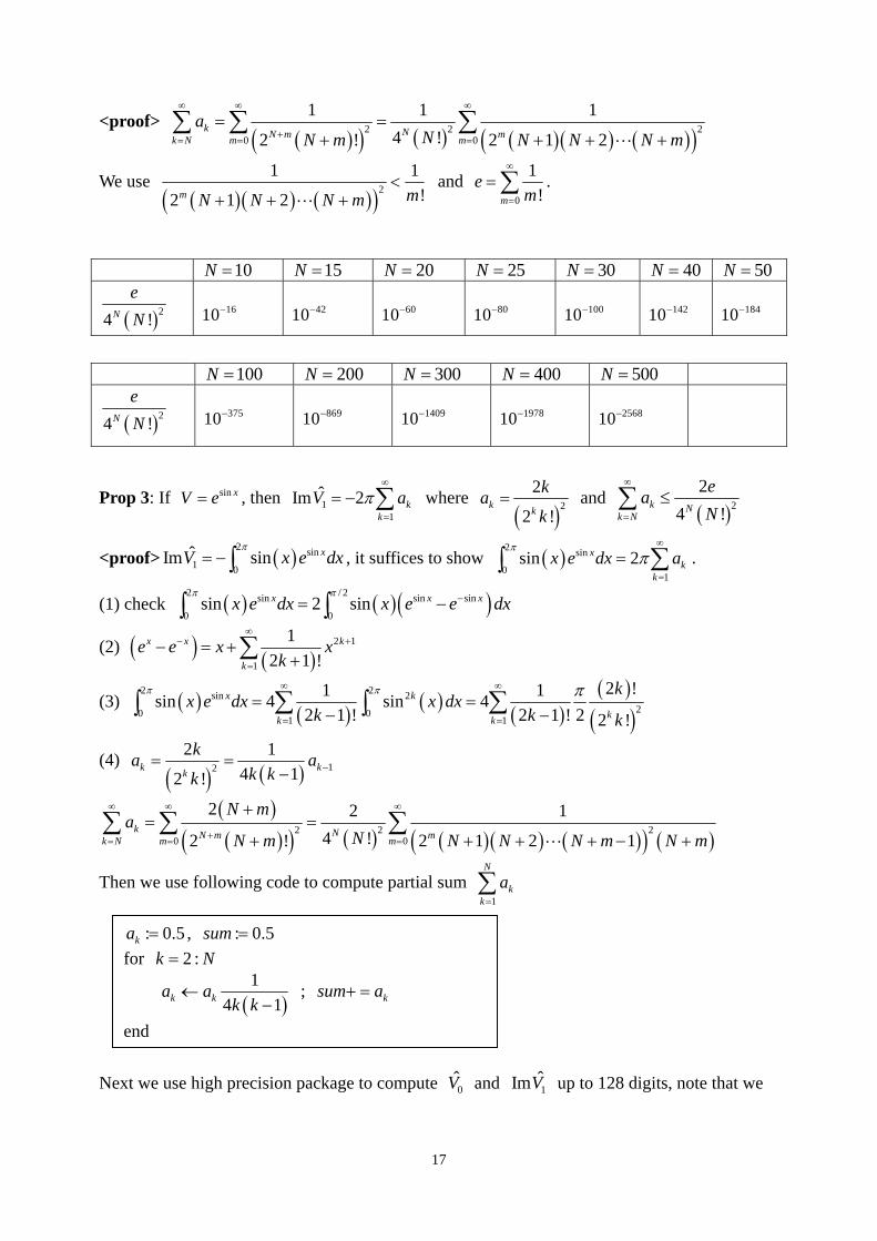
<proof> ( )( ) ( ) ( )( ) ( )( )2 2
0 0
1 1 14 !2 ! 2 1 2
k NN m mk N m ma
NN m N N N m
∞ ∞ ∞
+= = =
= =+ + +
∑ ∑ ∑ 2+
We use ( )( ) ( )( )2
1 1!2 1 2m mN N N m
<+ + +
and 0
1!m m
∞
=
=e ∑ .
10N = 15N = 20N = 25N = 30N = 40N = 50N =
( )24 !N
eN
1610−
4210−
6010−
8010−
10010−
14210−
18410−
100N = 200N = 300N = 400N = 500N =
( )24 !N
eN
37510−
86910−
140910−
197810−
256810−
Prop 3: If , then sin xV e= 11
ˆIm 2 kk
V π∞
=
= − a∑ where ( )2
2
2 !k k
kak
= and ( )22
4 !k N
k N
eaN
∞
=
≤∑
<proof> , it suffices to show ( )2 sin
1 0ˆIm sin xV x e
π= −∫ dx ( )
2 sin
01
sin 2xk
kx e dx a
ππ
∞
=
= ∑∫ .
(1) check ( ) ( )( )2 / 2sin sin sin
0 0sin 2 sinx x xx e dx x e e dx
π π −= −∫ ∫
(2) ( ) ( )2 1
1
12 1 !
x x k
ke e x x
k
∞− +
=
− = ++∑
(3) ( ) ( ) ( ) ( )( )( )
2 2sin 220 0
1 1
2 !1 1sin 4 sin 42 1 ! 2 1 ! 2 2 !
x k
kk k
kx e dx x dx
k k k
π π π∞ ∞
= =
= =− −∑ ∑∫ ∫
(4) ( ) ( ) 12
2 14 12 !
k kk
ka ak kk
−= =−
( )( )( ) ( ) ( )( ) ( )( ) ( )
2 2 20 0
2 2 14 !2 ! 2 1 2 1
k NN m mk N m m
N ma
NN m N N N m N m
∞ ∞ ∞
+= = =
+= =
+ + + + −∑ ∑ ∑
+
Then we use following code to compute partial sum 1
N
kk
a=∑
: 0.5ka = , : 0.5sum =for 2 :k N=
( )1
4 1k ka ak k
←−
; ksum a+ =
end
Next we use high precision package to compute and up to 128 digits, note that we 0̂V 1̂ImV
17

use to stabilize partial sum 42N ≥1
N
kk
a=∑ .
0̂V = 7.9549265210128452 7451321966532939 4328161342771816 6385734005959553 8336060816469466 6995137357228568 7741332170437587 4113888148503023e0
1̂ImV = -3.5509993784243618 9375715307444414 5068885827761984 4655200625893475 7625209545877072 0368124285904632 7616425367512080 1404294198552668e0 Table 7: We use high precision package with 1000 digits to compute and estimate
convergence order of , defined by
k̂V
k̂V ( )1
k̂ m kVk
= .
Source code: F:\course\2008spring\spectral_method\cxx_example\chap1 ( )m k
( )m k
ReV(0) = 7.9549265210128453e0 ImV(1) = -3.5509993784243619e0
ReV(2) = -8.5292776416412149e-1 ImV(3) = 1.3928832176787595e-1
ReV(4) = 1.7197833556865812e-2 ImV(5) = -1.7056533129494463e-3
ReV(6) = -1.4130042737134921e-4 4.94744 ImV(7) = 1.0048184493255820e-5 5.914
ReV(8) = 6.2584446576772422e-7 6.86923 ImV(9) = -3.4673040972232835e-8 7.81773
ReV(10) = -1.7297282675331887e-9 8.76202 ImV(11) = 7.8475621569060340e-11 9.70361
ReV(12) = 3.2645930138612418e-12 10.6434 ImV(13) = -1.2538923639053624e-13 11.582
ReV(14) = -4.4728677072995018e-15 12.5199 ImV(15) = 1.4894058615019287e-16 13.4573
ReV(16) = 4.6501227937157073e-18 14.3944 ImV(17) = -1.3665675129023628e-19 15.3313
ReV(18) = -3.7932498476738764e-21 16.2682 ImV(19) = 9.9756773976728090e-23 17.2051
ReV(20) = 2.4924365582089317e-24 18.1421 ImV(21) = -5.9311648370821361e-26 19.0792
ReV(22) = -1.3473266344345731e-27 20.0164 ImV(23) = 2.9276455700143845e-29 20.9539
ReV(24) = 6.0967222795625615e-31 21.8915 ImV(25) = -1.2188758243549561e-32 22.8293
ReV(26) = -2.3431577877807459e-34 23.7674 ImV(27) = 4.3377470896829986e-36 24.7056
ReV(28) = 7.7435935192659899e-38 25.6441 ImV(29) = -1.3347188940443096e-39 26.5828
ReV(30) = -2.2239338089943938e-41 27.5217 ImV(31) = 3.5860864767329276e-43 28.4608
ReV(32) = 5.6019341997869982e-45 29.4002 ImV(33) = -8.4858886924868411e-47 30.3397
ReV(34) = -1.2476627456831309e-48 31.2795 ImV(35) = 1.7820218415512617e-50 32.2195
ReV(36) = 2.4745659724766378e-52 33.1597 ImV(37) = -3.3434136808250048e-54 34.1001
ReV(38) = -4.3984866613426193e-56 35.0407 ImV(39) = 5.6381820461407180e-58 35.9815
ReV(40) = 7.0466535285927712e-60 36.9225 ImV(41) = -8.5922326650106772e-62 37.8637
ReV(42) = -1.0227432840158852e-63 38.805 ImV(43) = 1.1890792772412452e-65 39.7466
ReV(44) = 1.3510558841438762e-67 40.6883 ImV(45) = -1.5009919463409708e-69 41.6302
ReV(46) = -1.6313243700245210e-71 42.5723 ImV(47) = 1.7352591841154628e-73 43.5146
18

ReV(48) = 1.8073695598597204e-75 44.457 ImV(49) = -1.8440665013114252e-77 45.3996
ReV(50) = -1.8438857452372014e-79 46.3424 ImV(51) = 1.8075607422380681e-81 47.2853
ReV(52) = 1.7378815437191885e-83 48.2283 ImV(53) = -1.6393677011213502e-85 49.1716
ReV(54) = -1.5178053055730738e-87 50.1149 ImV(55) = 1.3797110243049970e-89 51.0584
ReV(56) = 1.2317883757703079e-91 52.0021 ImV(57) = -1.0804344225222833e-93 52.9459
ReV(58) = -9.3134094904861371e-96 53.8899 ImV(59) = 7.8921625891422459e-98 54.8339
ReV(60) = 6.5763529828695323e-100 55.7782 ImV(61) = -5.3900969880710571e-102 56.7225
ReV(62) = -4.3465742284267052e-104 57.667 ImV(63) = 3.4494482194268623e-106 58.6116
ReV(64) = 2.6947194885863902e-108 59.5563 ImV(65) = -2.0727403628291311e-110 60.5012
ReV(66) = -1.5701690851976058e-112 61.4462 ImV(67) = 1.1717036829142283e-114 62.3913
ReV(68) = 8.6150092539842003e-117 63.3365 ImV(69) = -6.2424372377078596e-119 64.2819
ReV(70) = -4.4586594735415350e-121 65.2273 ImV(71) = 3.1397474971062253e-123 66.1729
ReV(72) = 2.1802765069509171e-125 67.1186 ImV(73) = -1.4932709690467884e-127 68.0644
ReV(74) = -1.0089214260595890e-129 69.0102 ImV(75) = 6.7258478596712626e-132 69.9562
ReV(76) = 4.4247108899611723e-134 70.9024 ImV(77) = -2.8730693028074481e-136 71.8486
ReV(78) = -1.8416363770214422e-138 72.7949 ImV(79) = 1.1655465399828615e-140 73.7413
ReV(80) = 7.2843848521037795e-143 74.6878 ImV(81) = -4.4963646256784895e-145 75.6344
ReV(82) = -2.7415850462649380e-147 76.5811 ImV(83) = 1.6514980399108078e-149 77.5279
ReV(84) = 9.8300012997093223e-152 78.4748 ImV(85) = -5.7821559641664032e-154 79.4218
ReV(86) = -3.3616062643676250e-156 80.3689 ImV(87) = 1.9318945408827106e-158 81.316
ReV(88) = 1.0976323170853944e-160 82.2633 ImV(89) = -6.1662812416461892e-163 83.2106
ReV(90) = -3.4256072372713951e-165 84.1581 ImV(91) = 1.8821455767799992e-167 85.1056
ReV(92) = 1.0228753179651741e-169 86.0532 ImV(93) = -5.4991724078868826e-172 87.0009
ReV(94) = -2.9250098213943509e-174 87.9486 ImV(95) = 1.5394366550286099e-176 88.8965
ReV(96) = 8.0176839992052904e-179 89.8444 ImV(97) = -4.1327181194190573e-181 90.7924
ReV(98) = -2.1084753231915019e-183 91.7405 ImV(99) = 1.0648596371350890e-185 92.6886
ReV(100) = 5.3241664025762733e-188 93.6369 ImV(101) = -2.6356619834325278e-190 94.5852
ReV(102) = -1.2919604256718823e-192 95.5336 ImV(103) = 6.2715061887867499e-195 96.482
ReV(104) = 3.0150781811827308e-197 97.4306 ImV(105) = -1.4357192666992787e-199 98.3792
ReV(106) = -6.7721114245441988e-202 99.3278 ImV(107) = 3.1644695908567913e-204 100.277
ReV(108) = 1.4650011066538491e-206 101.225 ImV(109) = -6.7200484477269938e-209 102.174
ReV(110) = -3.0545049364460404e-211 103.123 ImV(111) = 1.3758754570485746e-213 104.072
ReV(112) = 6.1421798204873893e-216 105.021 ImV(113) = -2.7177259399354918e-218 105.971
ReV(114) = -1.1919623317795924e-220 106.92 ImV(115) = 5.1823478021086980e-223 107.869
ReV(116) = 2.2337294591867709e-225 108.818 ImV(117) = -9.5456795389410712e-228 109.768
ReV(118) = -4.0447074560274482e-230 110.717 ImV(119) = 1.6994271629333847e-232 111.667
ReV(120) = 7.0808245992629515e-235 112.616 ImV(121) = -2.9259110276340004e-237 113.566
ReV(122) = -1.1991238867047224e-239 114.516 ImV(123) = 4.8744074477763628e-242 115.466
19
ReV(124) = 1.9654551737166463e-244 116.415 ImV(125) = -7.8616959079921701e-247 117.365
ReV(126) = -3.1196718603786482e-249 118.315 ImV(127) = 1.2281983797660650e-251 119.265
ReV(128) = 4.7975772843065435e-254 120.215 ImV(129) = -1.8594983589878912e-256 121.165
ReV(130) = -7.1518117784269494e-259 122.116 ImV(131) = 2.7296596884347195e-261 123.066
ReV(132) = 1.0339472798414659e-263 124.016 ImV(133) = -3.8869653249621741e-266 124.967
ReV(134) = -1.4503401527580714e-268 125.917 ImV(135) = 5.3715570542648909e-271 126.867
ReV(136) = 1.9748106550868906e-273 127.818 ImV(137) = -7.2072428548484198e-276 128.768
ReV(138) = -2.6112858423585874e-278 129.719 ImV(139) = 9.3929938718587938e-281 130.67
ReV(140) = 3.3545981842720248e-283 131.62 ImV(141) = -1.1895589712441229e-285 132.571
ReV(142) = -4.1885363598235693e-288 133.522 ImV(143) = 1.4645054229194620e-290 134.473
ReV(144) = 5.0850273907962369e-293 135.424 ImV(145) = -1.7534370145803019e-295 136.375
ReV(146) = -6.0048513361321557e-298 137.326 ImV(147) = 2.0424429712458045e-300 138.277
ReV(148) = 6.9000669490463556e-303 139.228 ImV(149) = -2.3154328083236962e-305 140.179
ReV(150) = -7.7180241741020677e-308 141.13 ImV(151) = 2.5556093075861283e-310 142.082
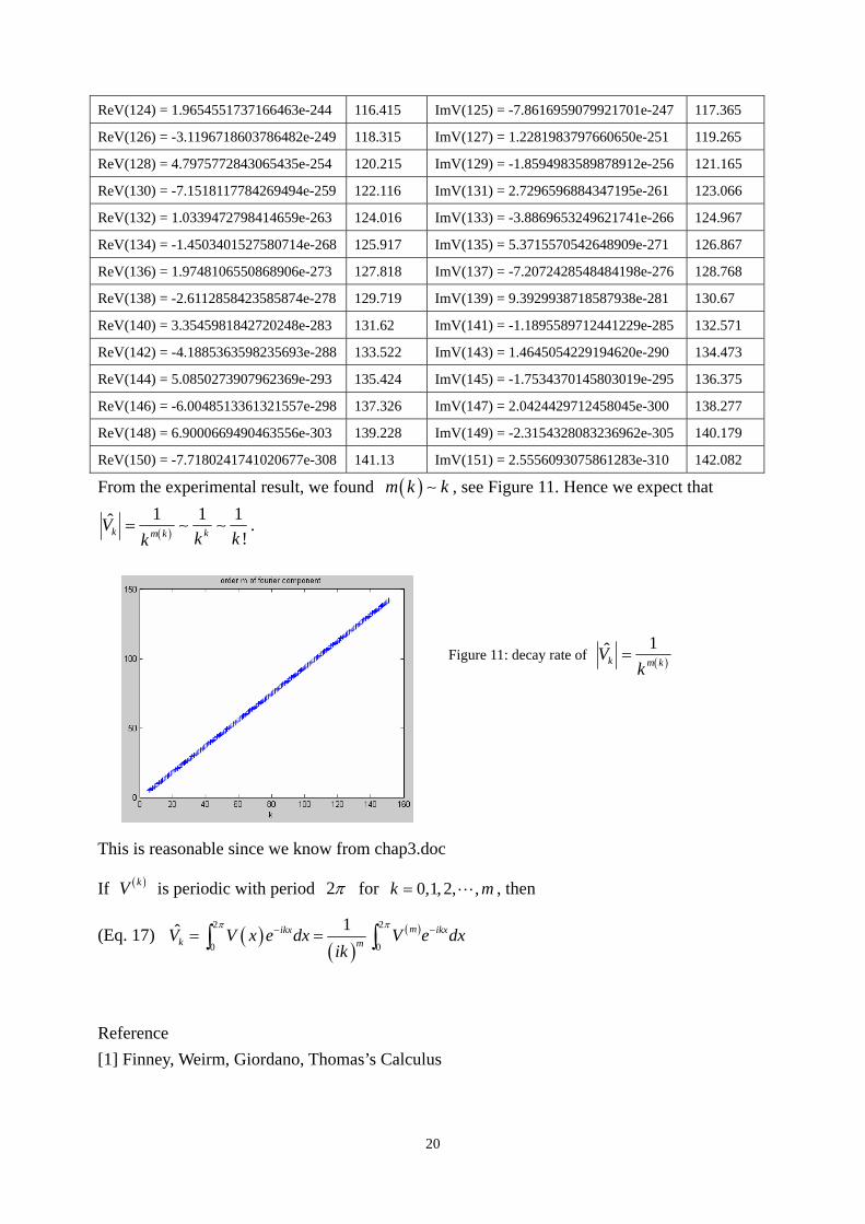
From the experimental result, we found ( )m k k∼ , see Figure 11. Hence we expect that
( )1 1ˆ
!k km kVk kk
= ∼ ∼ 1 .
Figure 11: decay rate of ( )1
k̂ m kVk
=
This is reasonable since we know from chap3.doc
If ( )kV is periodic with period 2π for 0,1, 2, ,k m= , then
(Eq. 17) ( )( )
( )2 2
0 0
1ˆ mikx ikxk mV V x e dx V e dx
ik
π π− −= =∫ ∫
Reference [1] Finney, Weirm, Giordano, Thomas’s Calculus
20