Embed Size (px)
Citation preview
CHAPTER 19: Single-Loop IMC Control
When I complete this chapter, I want to be able to do the following.
• Recognize that other feedback algorithms are possible
• Understand the IMC structure and how it provides the essential control features
• Tune an IMC controller
• Correctly select between PID and IMC
Outline of the lesson.
• Thought exercise for model-based control
• IMC structure
• Desired control features
• IMC algorithm and tuning
• Application guidelines
CHAPTER 19: Single-Loop IMC Control
CHAPTER 19: Single-Loop IMC Control
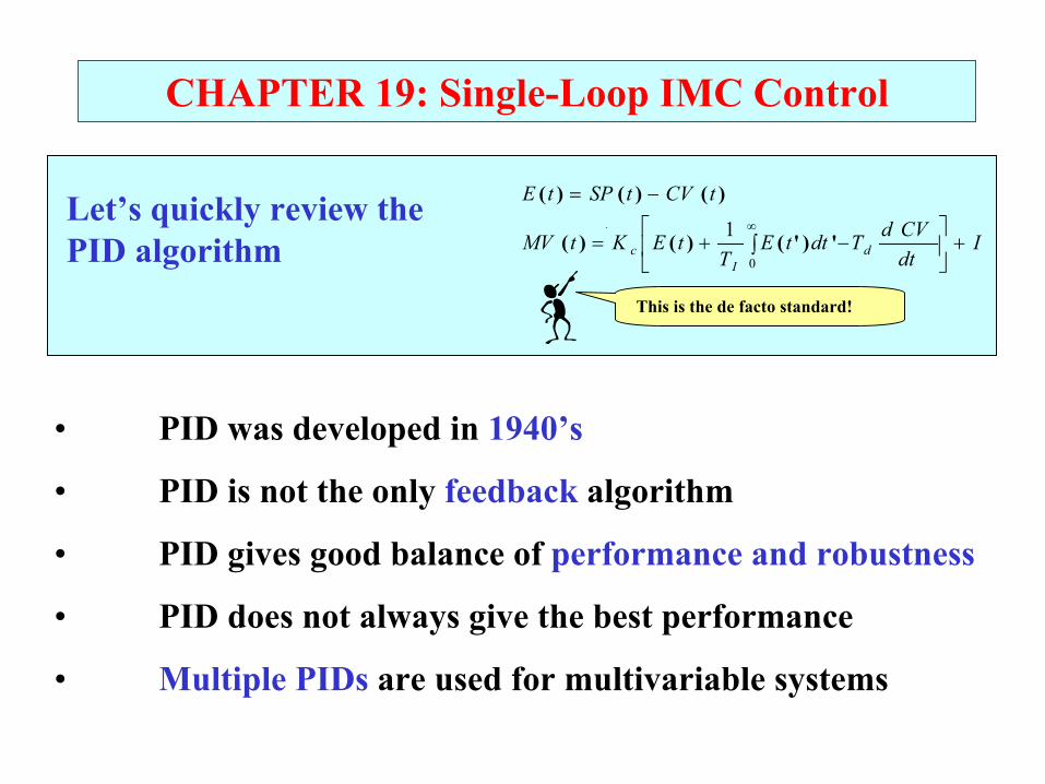
IdtCVdTdttE
TtEKtMV
tCVtSPtE
dI
c +
∫ −+=
−=∞
0
1 ')'()()(
)()()(
This is the de facto standard!
Let’s quickly review the PID algorithm
• PID was developed in 1940’s
• PID is not the only feedback algorithm
• PID gives good balance of performance and robustness
• PID does not always give the best performance
• Multiple PIDs are used for multivariable systems
CHAPTER 19: Single-Loop IMC Control
We will have another algorithm to learn!!!!
Let’s look ahead to the IMC structure and algorithm
• IMC was developed formally in 1980’s, but the ideas began in 1950’s
• IMC uses a process model explicitly
• IMC involves a different structure and controller
• IMC could replace PID, but we chose to retain PID unless an advantage exists
• A single “IMC” can be used for multivariable systems
CHAPTER 19: Single-Loop IMC Control
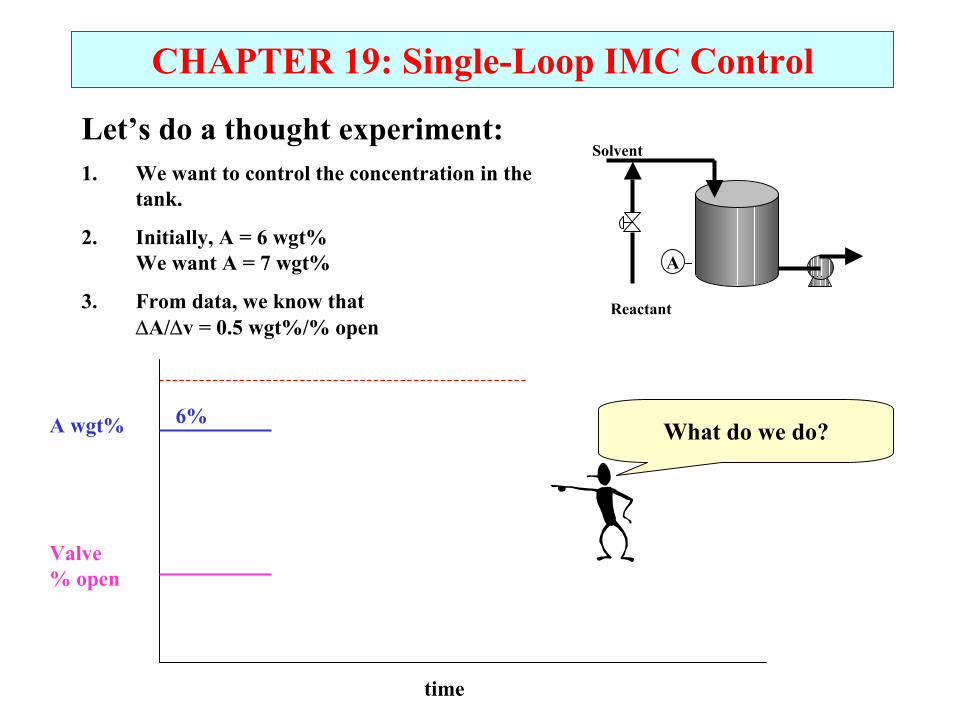
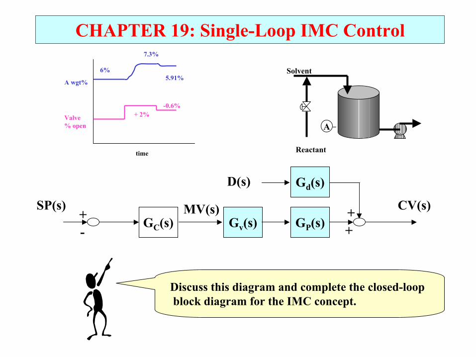
Let’s do a thought experiment:1. We want to control the concentration in the
tank.
2. Initially, A = 6 wgt%We want A = 7 wgt%
3. From data, we know that∆A/∆v = 0.5 wgt%/% open
A
Reactant
Solvent
time
Valve % open
A wgt% What do we do?6%
CHAPTER 19: Single-Loop IMC Control
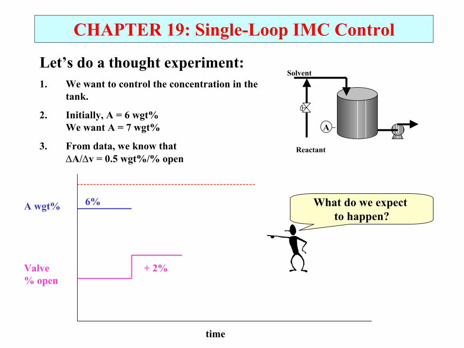
Let’s do a thought experiment:1. We want to control the concentration in the
tank.
2. Initially, A = 6 wgt%We want A = 7 wgt%
3. From data, we know that∆A/∆v = 0.5 wgt%/% open
A
Reactant
Solvent
time
Valve % open
A wgt% What do we expect to happen?
+ 2%
6%
CHAPTER 19: Single-Loop IMC Control
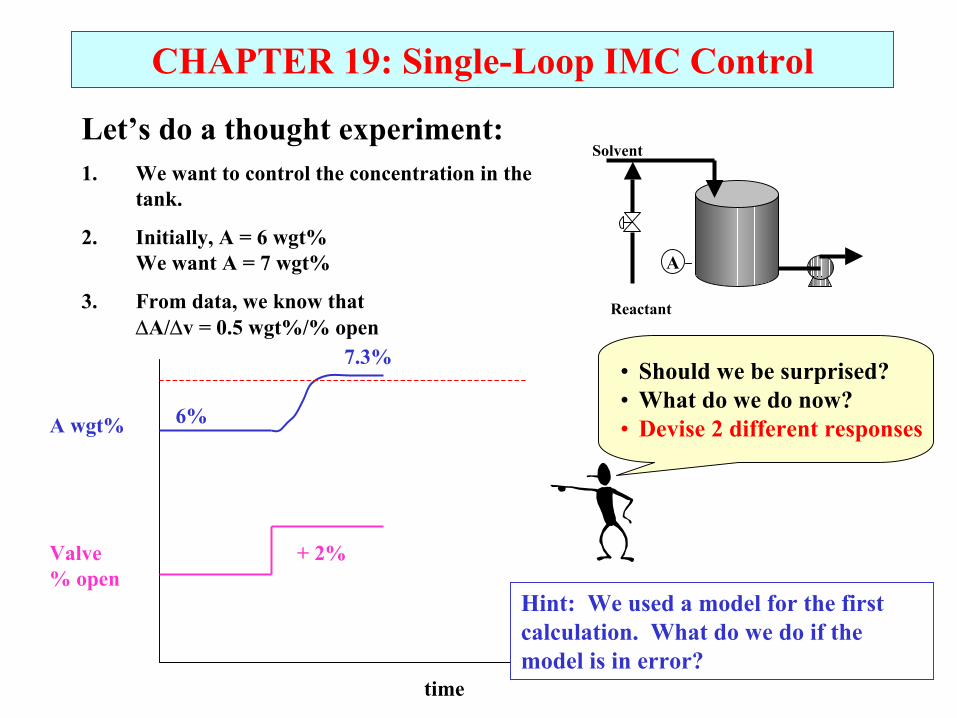
Let’s do a thought experiment:1. We want to control the concentration in the
tank.
2. Initially, A = 6 wgt%We want A = 7 wgt%
3. From data, we know that∆A/∆v = 0.5 wgt%/% open
A
Reactant
Solvent
time
Valve % open
A wgt%
• Should we be surprised?• What do we do now?• Devise 2 different responses
+ 2%
6%
7.3%
Hint: We used a model for the first calculation. What do we do if the model is in error?
CHAPTER 19: Single-Loop IMC Control
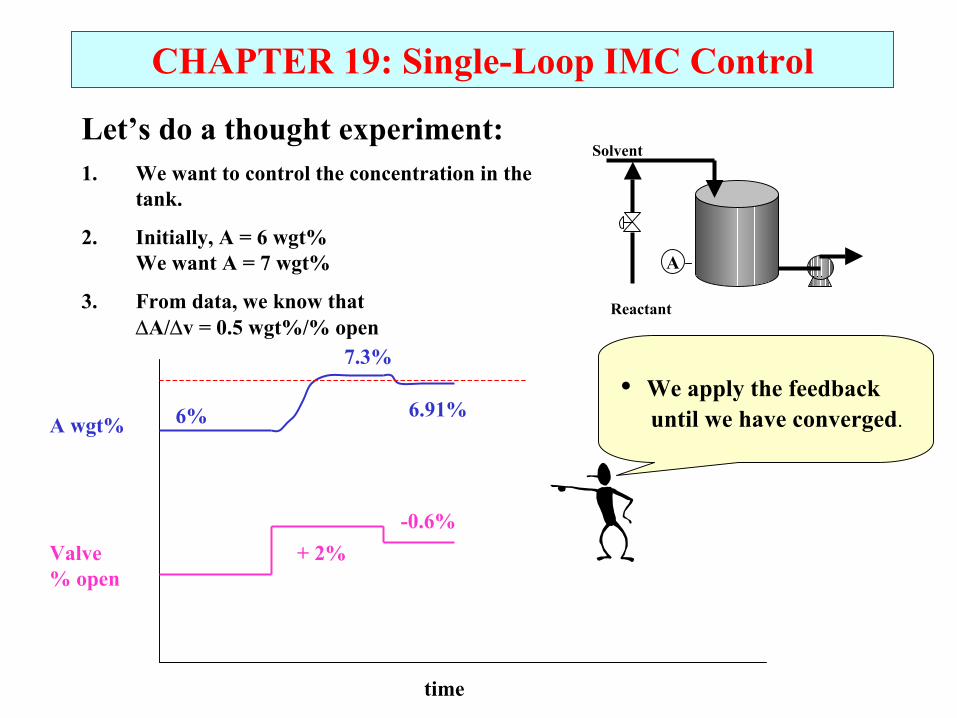
Let’s do a thought experiment:1. We want to control the concentration in the
tank.
2. Initially, A = 6 wgt%We want A = 7 wgt%
3. From data, we know that∆A/∆v = 0.5 wgt%/% open
A
Reactant
Solvent
time
Valve % open
A wgt%
• We apply the feedback until we have converged.
+ 2%
6%
7.3%
-0.6%
6.91%
CHAPTER 19: Single-Loop IMC Control
A
Reactant
Solvent
time
Valve % open
A wgt%
+ 2%
6%
7.3%
-0.6%
5.91%
Gd(s)
GP(s)Gv(s)GC(s)
D(s)
CV(s)SP(s) MV(s) ++
+-
Discuss this diagram and complete the closed-loopblock diagram for the IMC concept.
CHAPTER 19: Single-Loop IMC Control
A
Reactant
Solvent
time
Valve % open
A wgt%
+ 2%
6%
7.3%
-0.6%
5.91%
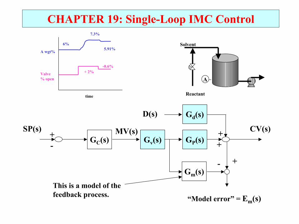
Gd(s)
GP(s)Gv(s)GC(s)
D(s)
CV(s)SP(s) MV(s) ++
+-
Gm(s)- +
“Model error” = Em(s)This is a model of the feedback process.
CHAPTER 19: Single-Loop IMC Control
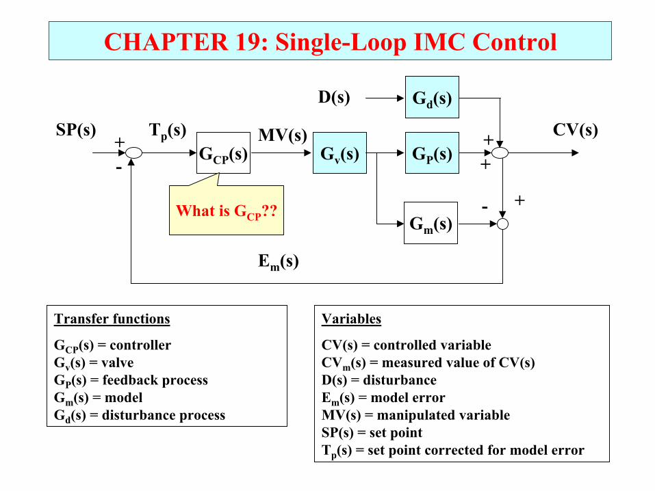
Gd(s)
GP(s)Gv(s)GCP(s)
D(s)
CV(s)SP(s) MV(s) ++
+-
Gm(s)- +
Em(s)
Tp(s)
Transfer functions
GCP(s) = controllerGv(s) = valve GP(s) = feedback processGm(s) = modelGd(s) = disturbance process
Variables
CV(s) = controlled variableCVm(s) = measured value of CV(s)D(s) = disturbanceEm(s) = model errorMV(s) = manipulated variableSP(s) = set pointTp(s) = set point corrected for model error
What is GCP??
CHAPTER 19: Single-Loop IMC Control
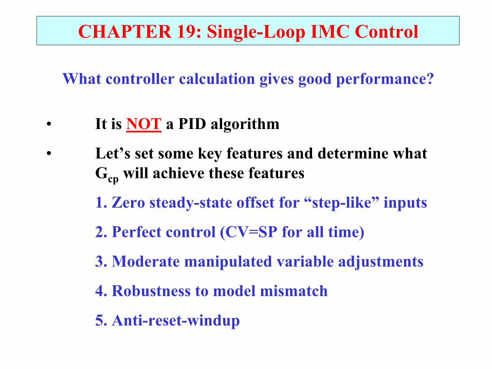
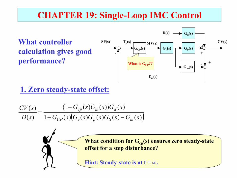
What controller calculation gives good performance?
• It is NOT a PID algorithm
• Let’s set some key features and determine what Gcp will achieve these features
1. Zero steady-state offset for “step-like” inputs
2. Perfect control (CV=SP for all time)
3. Moderate manipulated variable adjustments
4. Robustness to model mismatch
5. Anti-reset-windup
CHAPTER 19: Single-Loop IMC Control
What controller calculation gives good performance?
Gd(s)
GP(s)Gv(s)GCP(s)
D(s)
CV(s)SP(s) MV(s)++
+-
Gm(s)- +
Em(s)
Tp(s)
What is GCP??
( ))()()()()(1)())()(1(
)()(
sGsGsGsGsGsGsGsG
sDsCV
mSpvCP
dmcp
−+
−=
What condition for Gcp(s) ensures zero steady-stateoffset for a step disturbance?
Hint: Steady-state is at t = ∞.
1. Zero steady-state offset:
CHAPTER 19: Single-Loop IMC Control
What controller calculation gives good performance?
Gd(s)
GP(s)Gv(s)GCP(s)
D(s)
CV(s)SP(s) MV(s)++
+-
Gm(s)- +
Em(s)
Tp(s)
What is GCP??
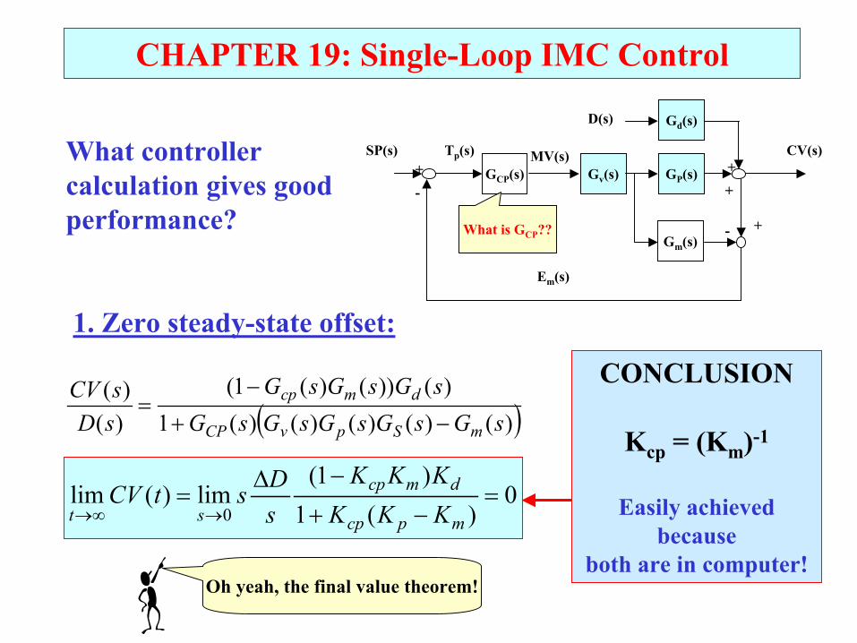
1. Zero steady-state offset:
0)(1
)1( lim)(lim
0=
−+
−∆=
→∞→ mpcp
dmcp
st KKKKKK
sDstCV
Oh yeah, the final value theorem!
CONCLUSION
Kcp = (Km)-1
Easily achieved because
both are in computer!
( ))()()()()(1)())()(1(
)()(
sGsGsGsGsGsGsGsG
sDsCV
mSpvCP
dmcp
−+
−=
CHAPTER 19: Single-Loop IMC Control
What controller calculation gives good performance?
Gd(s)
GP(s)Gv(s)GCP(s)
D(s)
CV(s)SP(s) MV(s)++
+-
Gm(s)- +
Em(s)
Tp(s)
What is GCP??
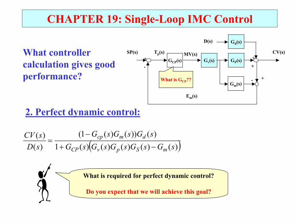
2. Perfect dynamic control:
What is required for perfect dynamic control?
Do you expect that we will achieve this goal?
( ))()()()()(1)())()(1(
)()(
sGsGsGsGsGsGsGsG
sDsCV
mSpvCP
dmcp
−+
−=
CHAPTER 19: Single-Loop IMC Control
What controller calculation gives good performance?
Gd(s)
GP(s)Gv(s)GCP(s)
D(s)
CV(s)SP(s) MV(s)++
+-
Gm(s)- +
Em(s)
Tp(s)
What is GCP??
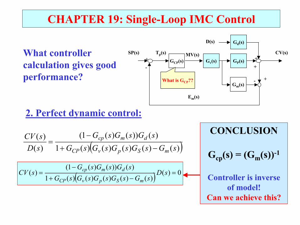
2. Perfect dynamic control:
( ) 0)()()()()()(1
)())()(1()( =
−+
−= sD
sGsGsGsGsGsGsGsG
sCVmSpvCP
dmcp
CONCLUSION
Gcp(s) = (Gm(s))-1
Controller is inverse of model!
Can we achieve this?
( ))()()()()(1)())()(1(
)()(
sGsGsGsGsGsGsGsG
sDsCV
mSpvCP
dmcp
−+
−=
CHAPTER 19: Single-Loop IMC Control
CONCLUSION
Gcp(s) = (Gm(s))-1
Controller is inverse of model!
Can we achieve this?
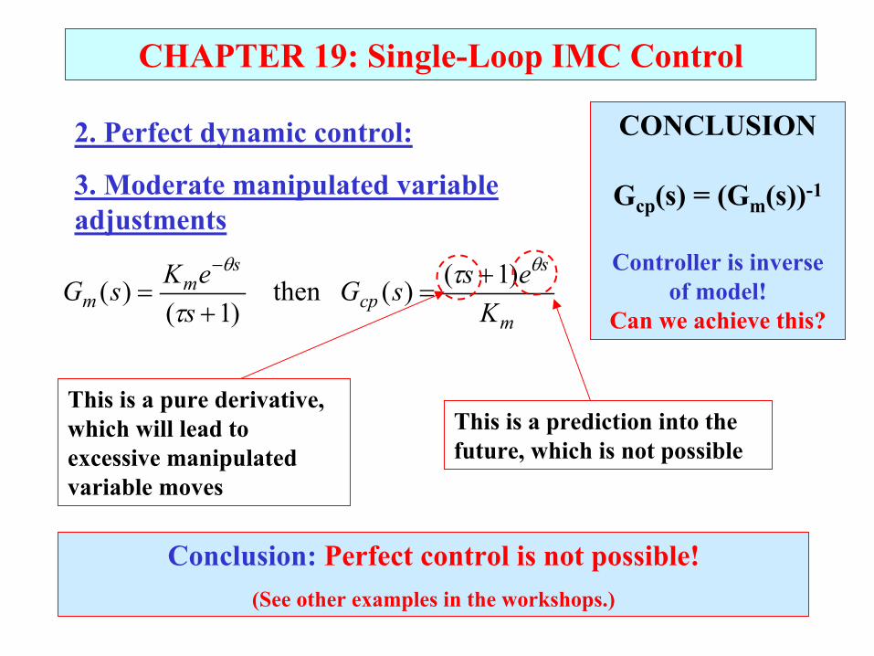
2. Perfect dynamic control:
3. Moderate manipulated variable adjustments
m
s
cp
sm
m KessG
seKsG
θθ ττ
)1()( then)1(
)( +=
+=
−
This is a pure derivative, which will lead to excessive manipulated variable moves
This is a prediction into the future, which is not possible
Conclusion: Perfect control is not possible! (See other examples in the workshops.)
CHAPTER 19: Single-Loop IMC Control
CONCLUSION
Gcp(s) = (Gm(s))-1
Controller is inverse of model!
Can we achieve this?
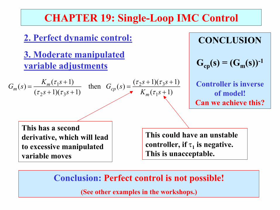
2. Perfect dynamic control:
3. Moderate manipulated variable adjustments
)1()1)(1()( then
)1)(1()1()(
1
32
32
1
+++
=++
+=
sKsssG
sssKsG
mcp
mm τ
ττττ
τ
This has a second derivative, which will lead to excessive manipulated variable moves
This could have an unstable controller, if τ1 is negative. This is unacceptable.
Conclusion: Perfect control is not possible! (See other examples in the workshops.)
CHAPTER 19: Single-Loop IMC Control
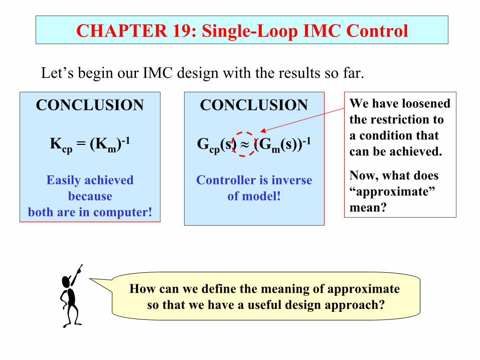
Let’s begin our IMC design with the results so far.
CONCLUSION
Kcp = (Km)-1
Easily achieved because
both are in computer!
CONCLUSION
Gcp(s) ≈ (Gm(s))-1
Controller is inverse of model!
We have loosened the restriction to a condition that can be achieved.
Now, what does “approximate” mean?
How can we define the meaning of approximate so that we have a useful design approach?
CHAPTER 19: Single-Loop IMC Control
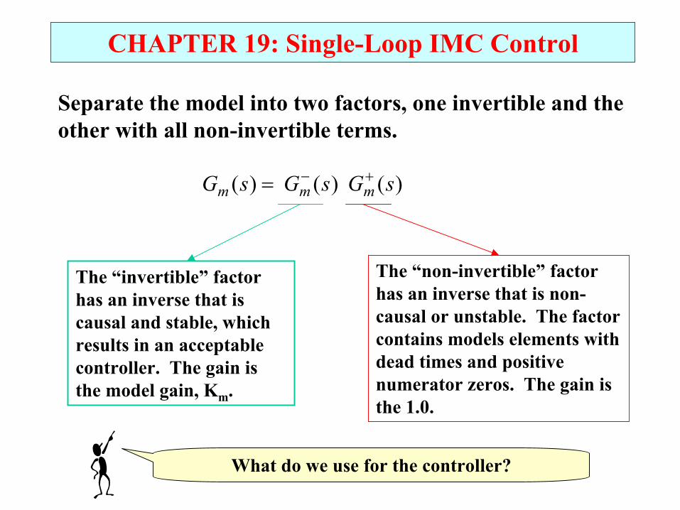
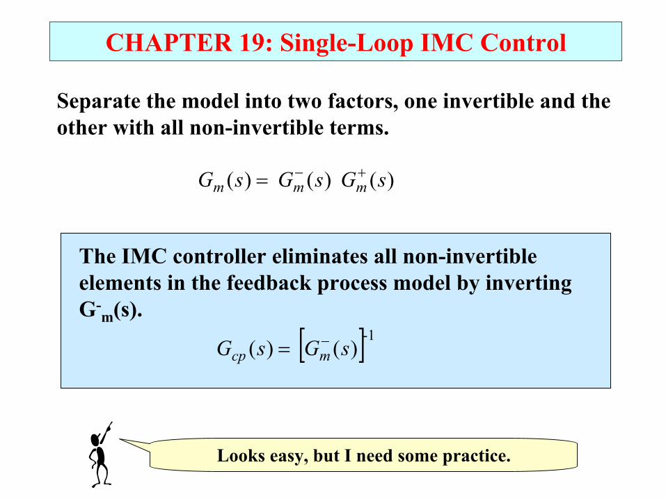
Separate the model into two factors, one invertible and the other with all non-invertible terms.
)( )( )( sGsGsG mmm+−=
The “invertible” factor has an inverse that is causal and stable, which results in an acceptable controller. The gain is the model gain, Km.
The “non-invertible” factor has an inverse that is non-causal or unstable. The factor contains models elements with dead times and positive numerator zeros. The gain is the 1.0.
What do we use for the controller?
CHAPTER 19: Single-Loop IMC Control
Separate the model into two factors, one invertible and the other with all non-invertible terms.
)( )( )( sGsGsG mmm+−=
Looks easy, but I need some practice.
The IMC controller eliminates all non-invertibleelements in the feedback process model by inverting G-
m(s).
[ ] )( )(-1
sGsG mcp−=
CHAPTER 19: Single-Loop IMC Control
solvent
pure A
AC
FS
FA
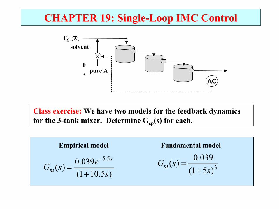
Class exercise: We have two models for the feedback dynamics for the 3-tank mixer. Determine Gcp(s) for each.
3)51(039.0)(s
sGm +=
)5.101(039.0)(
5.5
sesG
s
m +=
−
Empirical model Fundamental model
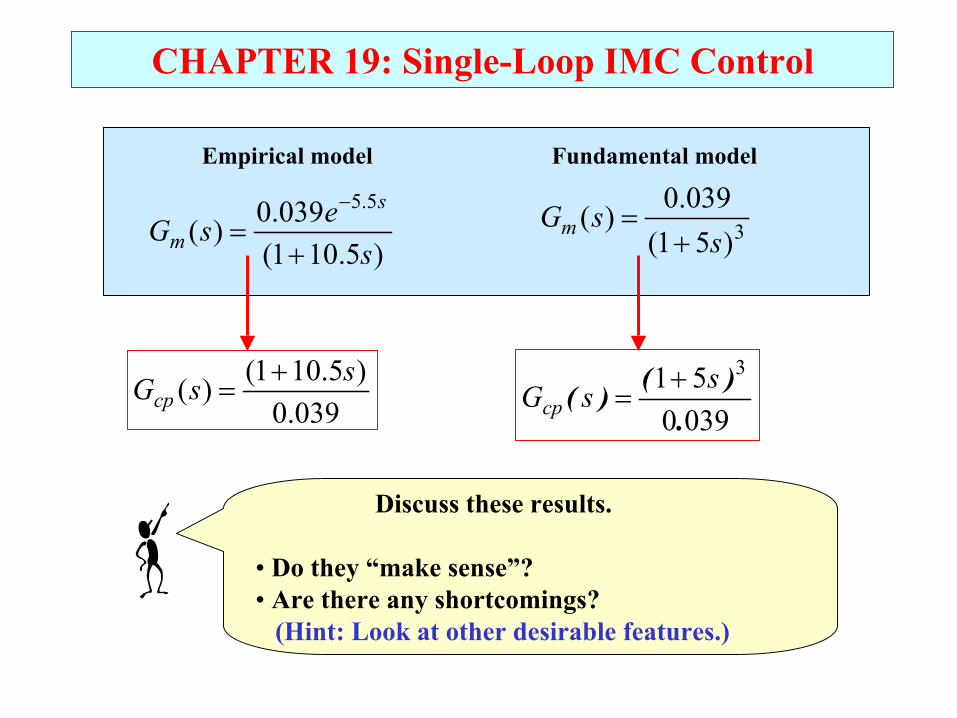
CHAPTER 19: Single-Loop IMC Control
3)51(039.0)(s
sGm +=
)5.101(039.0)(
5.5
sesG
s
m +=
−
Empirical model Fundamental model
039.0)5.101()( ssGcp
+=
039051 3
.)()( ssGcp
+=
Discuss these results.
• Do they “make sense”?• Are there any shortcomings?
(Hint: Look at other desirable features.)
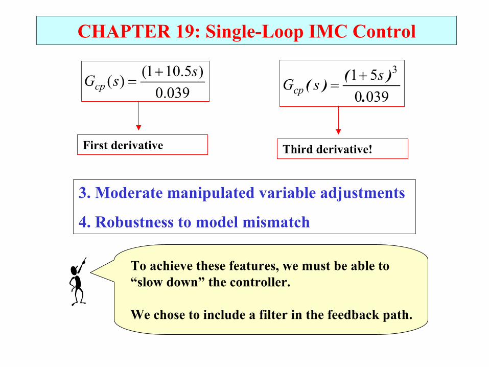
CHAPTER 19: Single-Loop IMC Control
039.0)5.101()( ssGcp
+=
039051 3
.)()( ssGcp
+=
First derivative Third derivative!
3. Moderate manipulated variable adjustments
4. Robustness to model mismatch
To achieve these features, we must be able to “slow down” the controller.
We chose to include a filter in the feedback path.
CHAPTER 19: Single-Loop IMC Control
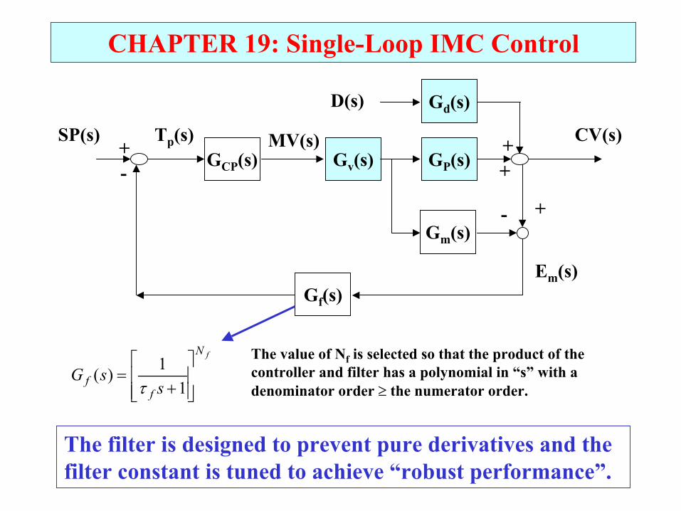
Gd(s)
GP(s)Gv(s)GCP(s)
D(s)
CV(s)SP(s) MV(s) ++
+-
Gm(s)- +
Em(s)
Tp(s)
Gf(s)
The filter is designed to prevent pure derivatives and the filter constant is tuned to achieve “robust performance”.
fN
ff ssG
+=
11)(
τ
The value of Nf is selected so that the product of the controller and filter has a polynomial in “s” with a denominator order ≥ the numerator order.
CHAPTER 19: Single-Loop IMC Control
3)51(039.0)(s
sGm +=
)5.101(039.0)(
5.5
sesG
s
m +=
−
Empirical model Fundamental model
039.0)5.101()( ssGcp
+=
039051 3
.)()( ssGcp
+=
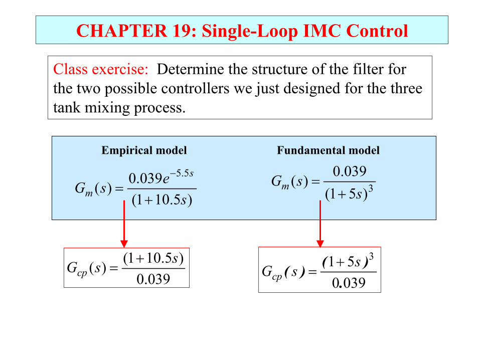
Class exercise: Determine the structure of the filter for the two possible controllers we just designed for the three tank mixing process.
CHAPTER 19: Single-Loop IMC Control
3)51(039.0)(s
sGm +=
)5.101(039.0)(
5.5
sesG
s
m +=
−
Empirical model Fundamental model
039.0)5.101()( ssGcp
+=
039051 3
.)()( ssGcp
+=
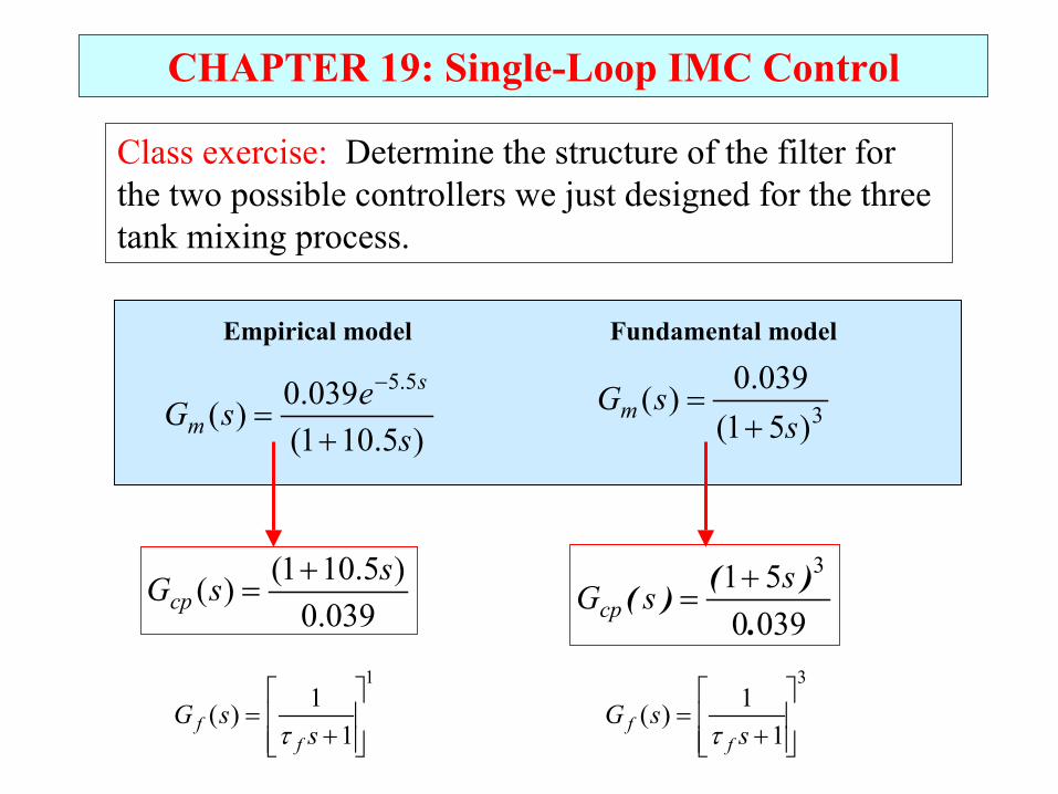
Class exercise: Determine the structure of the filter for the two possible controllers we just designed for the three tank mixing process.
1
11)(
+=
ssG
ff τ
3
11)(
+=
ssG
ff τ
CHAPTER 19: Single-Loop IMC Control
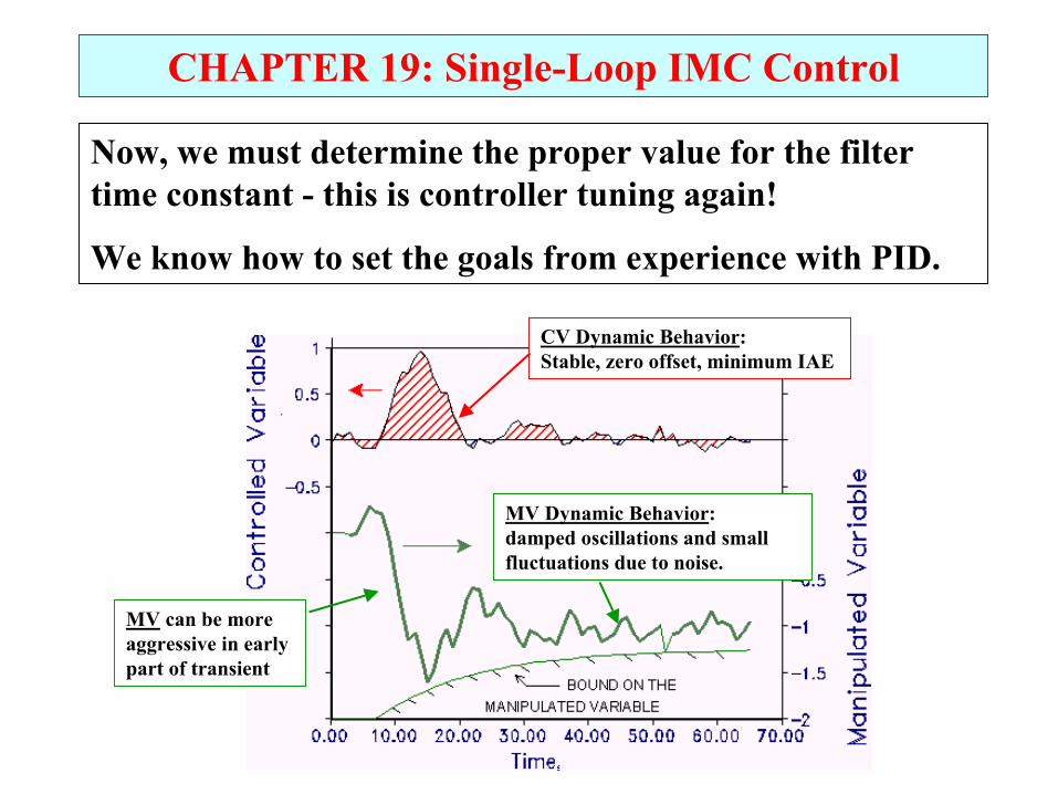
Now, we must determine the proper value for the filter time constant - this is controller tuning again!
We know how to set the goals from experience with PID.
CV Dynamic Behavior:Stable, zero offset, minimum IAE
MV Dynamic Behavior:damped oscillations and small fluctuations due to noise.
MV can be more aggressive in early part of transient
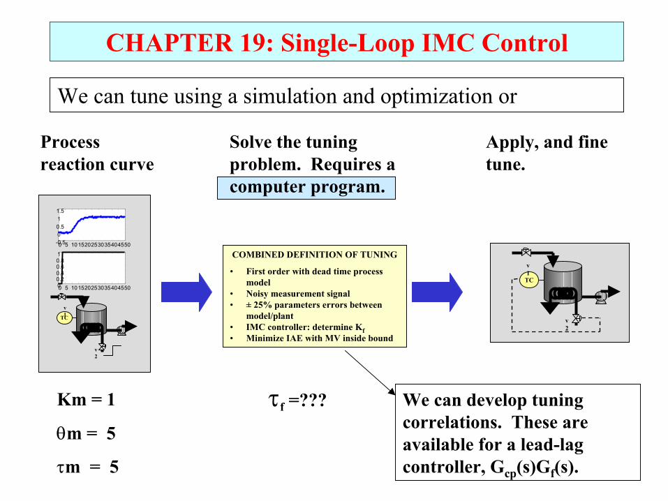
COMBINED DEFINITION OF TUNING
• First order with dead time process model
• Noisy measurement signal• ± 25% parameters errors between
model/plant• IMC controller: determine Kf• Minimize IAE with MV inside bound
Km = 1
θm = 5
τm = 5
TC
v1
v2
0 5 101520253035404550-0.500.511.5
0 5 10152025303540455000.20.40.60.81
TC
v1
v2
τf =???
Process reaction curve
Solve the tuning problem. Requires a computer program.
Apply, and fine tune.
CHAPTER 19: Single-Loop IMC Control
We can tune using a simulation and optimization or
We can develop tuning correlations. These are available for a lead-lag controller, Gcp(s)Gf(s).
CHAPTER 19: Single-Loop IMC Control
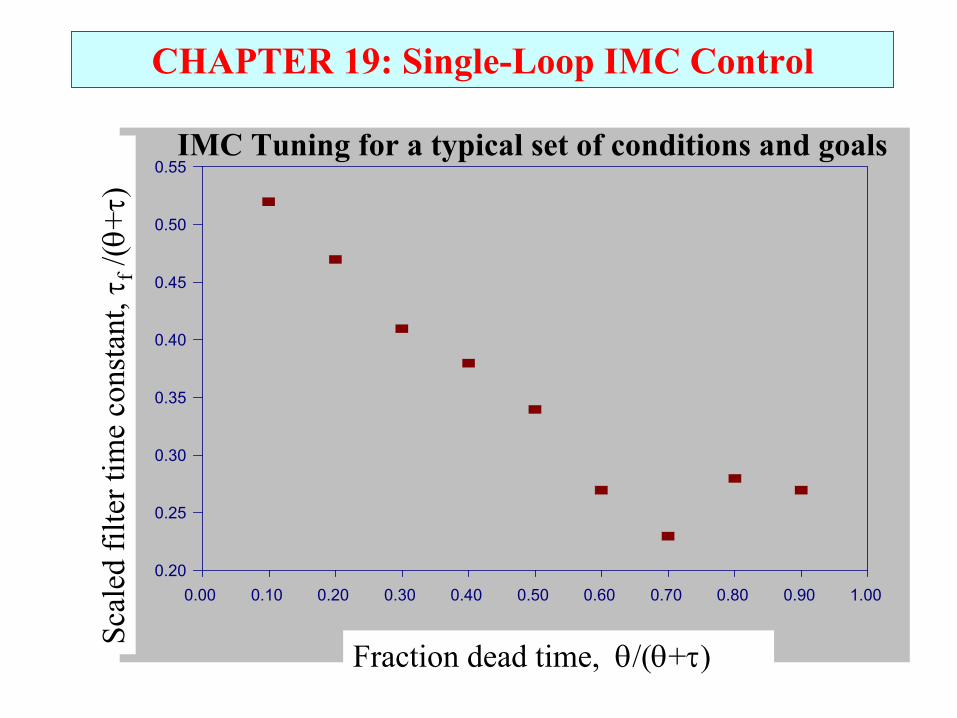
0.20
0.25
0.30
0.35
0.40
0.45
0.50
0.55
0.00 0.10 0.20 0.30 0.40 0.50 0.60 0.70 0.80 0.90 1.00
Fraction dead time, θ/(θ+τ)
Scal
ed fi
lter t
ime
cons
tant
, τf/(θ
+τ)
IMC Tuning for a typical set of conditions and goals
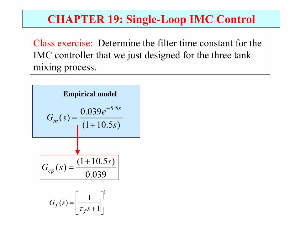
CHAPTER 19: Single-Loop IMC Control
)5.101(039.0)(
5.5
sesG
s
m +=
−
Empirical model
039.0)5.101()( ssGcp
+=
Class exercise: Determine the filter time constant for the IMC controller that we just designed for the three tank mixing process.
1
11)(
+=
ssG
ff τ
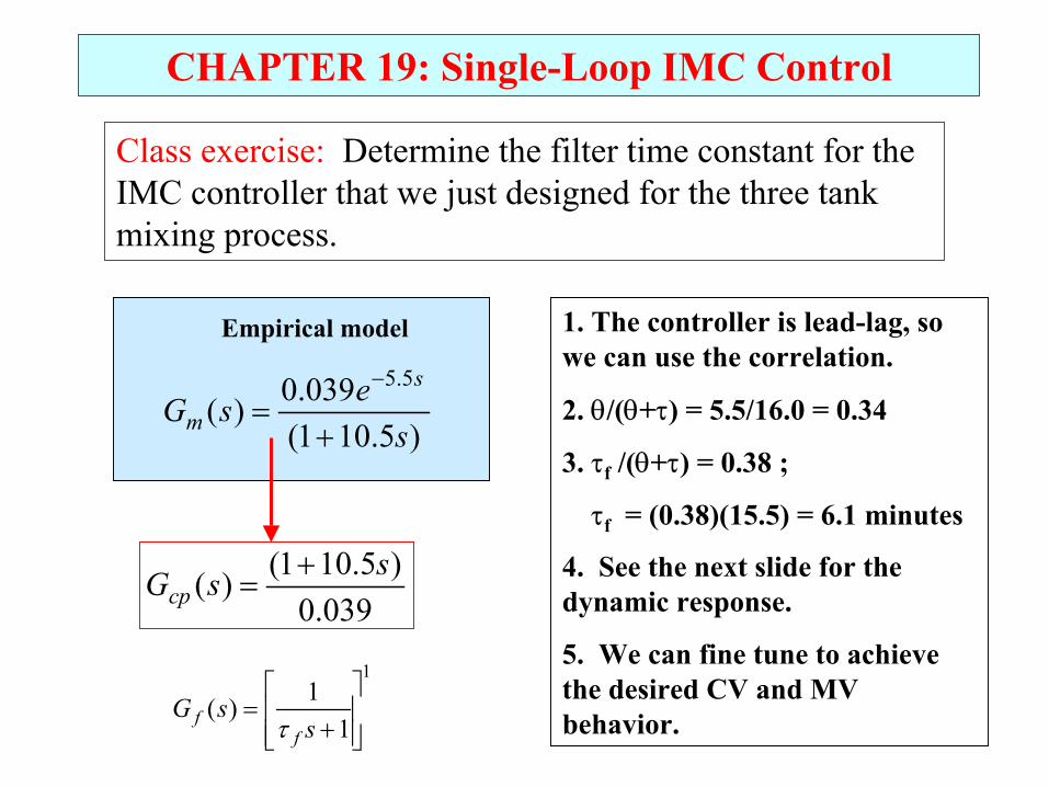
CHAPTER 19: Single-Loop IMC Control
)5.101(039.0)(
5.5
sesG
s
m +=
−
Empirical model
039.0)5.101()( ssGcp
+=
Class exercise: Determine the filter time constant for the IMC controller that we just designed for the three tank mixing process.
1
11)(
+=
ssG
ff τ
1. The controller is lead-lag, so we can use the correlation.
2. θ/(θ+τ) = 5.5/16.0 = 0.34
3. τf /(θ+τ) = 0.38 ;
τf = (0.38)(15.5) = 6.1 minutes
4. See the next slide for the dynamic response.
5. We can fine tune to achieve the desired CV and MV behavior.
CHAPTER 19: Single-Loop IMC Control
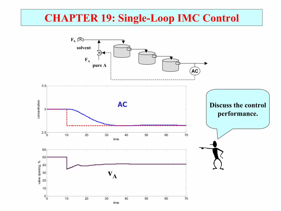
0 10 20 30 40 50 60 702.5
3
3.5
time
conc
entra
tion
0 10 20 30 40 50 60 700
10
20
30
40
50
60
time
valv
e op
enin
g, %
solvent
pure AAC
FS
FA
AC
vA
Discuss the controlperformance.
CHAPTER 19: Single-Loop IMC Control
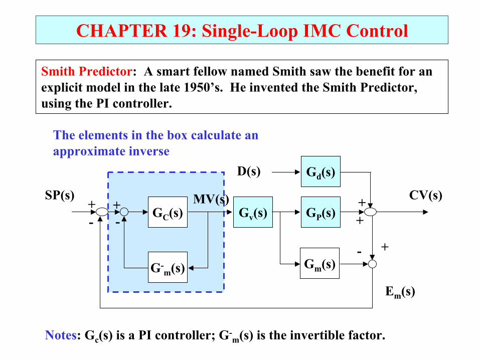
Gd(s)
GP(s)Gv(s)GC(s)
D(s)
CV(s)SP(s) MV(s) ++
+-
Gm(s)- +
Em(s)
Smith Predictor: A smart fellow named Smith saw the benefit for an explicit model in the late 1950’s. He invented the Smith Predictor, using the PI controller.
G-m(s)
-+
The elements in the box calculate an approximate inverse
Notes: Gc(s) is a PI controller; G-m(s) is the invertible factor.
CHAPTER 19: Single-Loop IMC Control
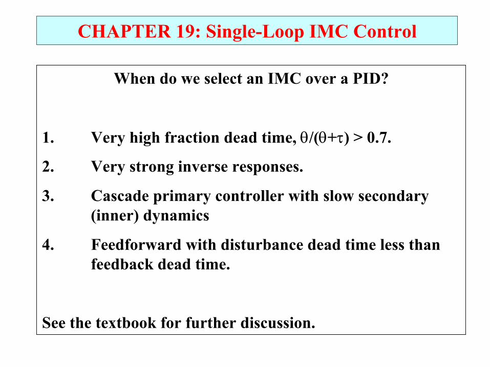
When do we select an IMC over a PID?
1. Very high fraction dead time, θ/(θ+τ) > 0.7.
2. Very strong inverse responses.
3. Cascade primary controller with slow secondary (inner) dynamics
4. Feedforward with disturbance dead time less than feedback dead time.
See the textbook for further discussion.
CHAPTER 19: IMC CONTROL WORKSHOP 1
0 50 100 150-0.4
-0.2
0
0.2
0.4
0.6
0.8
1
time
conc
entra
tion
0 50 100 150-2
-1.5
-1
-0.5
0
time
man
ipul
ated
flow
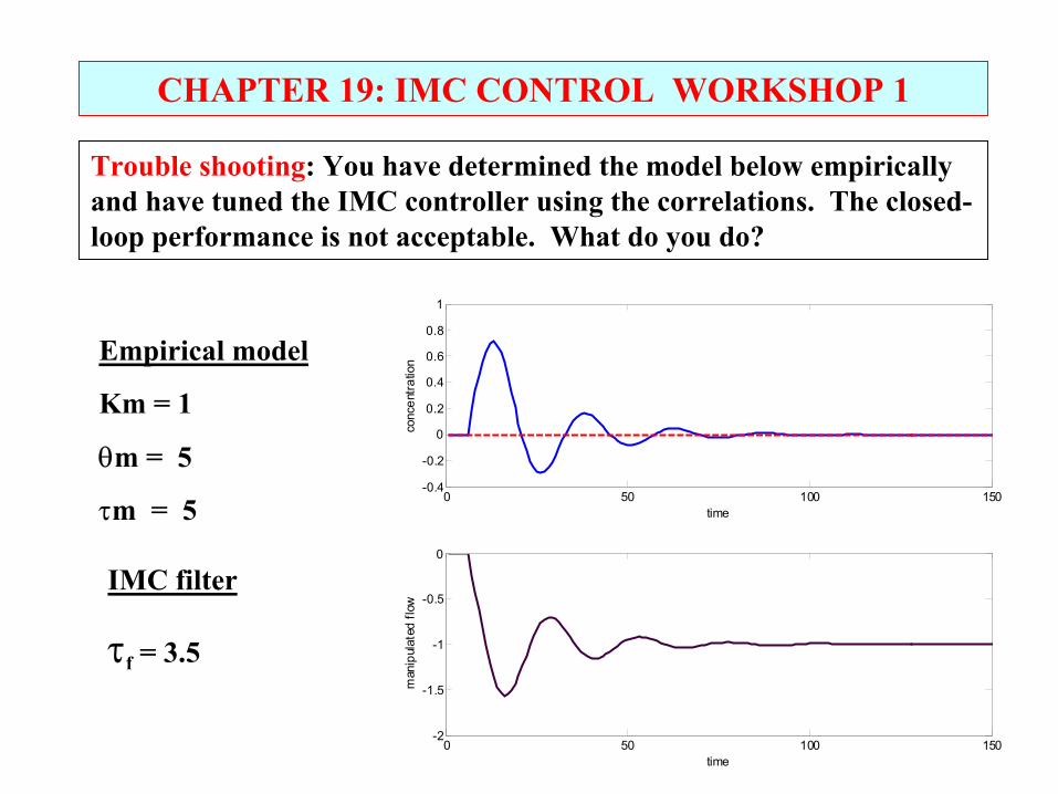
Empirical model
Km = 1
θm = 5
τm = 5
IMC filter
τf = 3.5
Trouble shooting: You have determined the model below empirically and have tuned the IMC controller using the correlations. The closed-loop performance is not acceptable. What do you do?
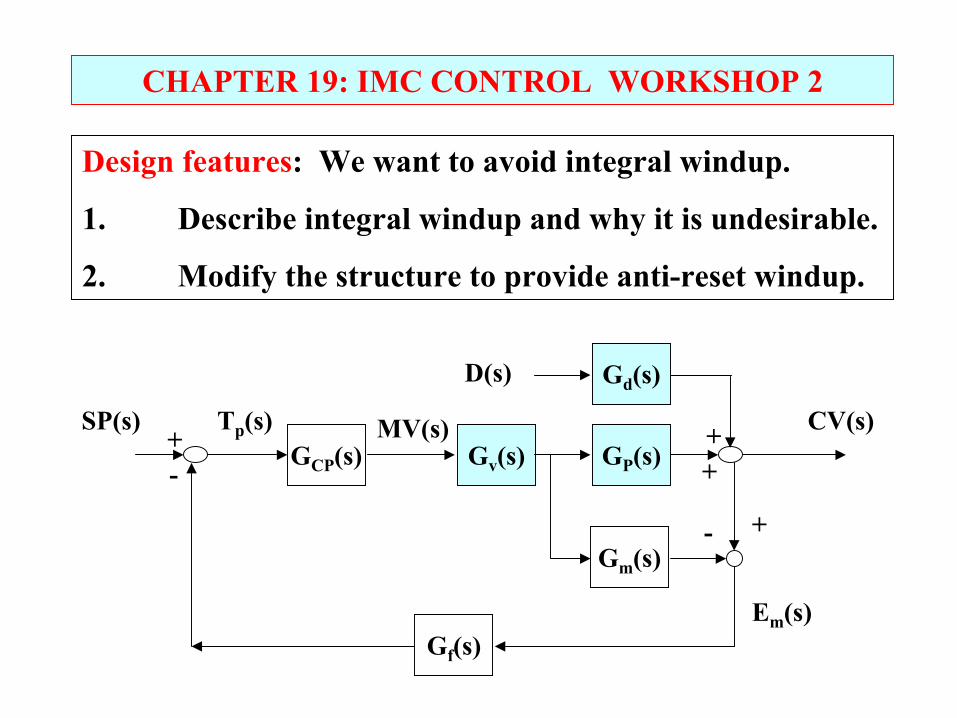
CHAPTER 19: IMC CONTROL WORKSHOP 2
Gd(s)
GP(s)Gv(s)GCP(s)
D(s)
CV(s)SP(s) MV(s) ++
+-
Gm(s)- +
Em(s)
Tp(s)
Gf(s)
Design features: We want to avoid integral windup.
1. Describe integral windup and why it is undesirable.
2. Modify the structure to provide anti-reset windup.
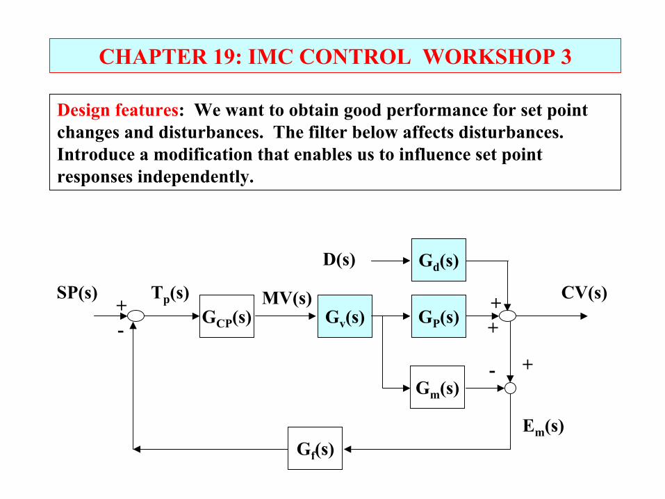
CHAPTER 19: IMC CONTROL WORKSHOP 3
Gd(s)
GP(s)Gv(s)GCP(s)
D(s)
CV(s)SP(s) MV(s) ++
+-
Gm(s)- +
Em(s)
Tp(s)
Gf(s)
Design features: We want to obtain good performance for set point changes and disturbances. The filter below affects disturbances. Introduce a modification that enables us to influence set point responses independently.
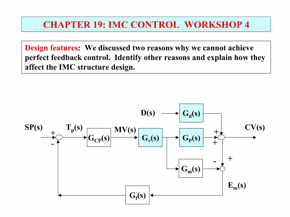
CHAPTER 19: IMC CONTROL WORKSHOP 4
Gd(s)
GP(s)Gv(s)GCP(s)
D(s)
CV(s)SP(s) MV(s) ++
+-
Gm(s)- +
Em(s)
Tp(s)
Gf(s)
Design features: We discussed two reasons why we cannot achieve perfect feedback control. Identify other reasons and explain how they affect the IMC structure design.
Lot’s of improvement, but we need some more study!• Read the textbook• Review the notes, especially learning goals and workshop• Try out the self-study suggestions• Naturally, we’ll have an assignment!
When I complete this chapter, I want to be able to do the following.
• Recognize that other feedback algorithms are possible
• Understand the IMC structure and how it provides the essential control features
• Tune an IMC controller
• Correctly select between PID and IMC
CHAPTER 19: Single-Loop IMC Control
CHAPTER 19: LEARNING RESOURCES
• SITE PC-EDUCATION WEB - Tutorials (Chapter 19)
• The Textbook, naturally, for many more examples.
• Addition information on IMC control is given in the following reference.
Brosilow, C. and B. Joseph, Techniques of Model-Based Control, Prentice-Hall, Upper Saddle River, 2002
CHAPTER 19: SUGGESTIONS FOR SELF-STUDY
1. Discuss the similarities and differences between IMC and Smith Predictor algorithms
2. Develop the equations that would be solved for a digital implementation of the IMC controller for the three-tank mixer.
3. Select a feedback control example in the textbook and determine the IMC tuning for this process.
4. Find a feedback control example in the textbook for which IMC is a better choice than PID.
5. Explain how you would implement a digital algorithm to provide good control for the process in Example 19.8 experiencing the flow variation described.