Chapter 6 Microwave ResonatorsChapter 6 Microwave ResonatorsPart I1. Series and Parallel Resonant Circuits2. Loss and Q Factor of a Resonant Circuit3. Various Waveguide Resonators4. Coupling to a Lossy Resonator

Part II Time-Domain Analysis of Open Cavities

Part III Spectral-Domain Analysis of Open Cavities

1

6.1 Series and Parallel Resonant Circuits(1) Series Resonant Circuit

1

2* 21 1 2

in

ini i l i

Z R j L j CP

P VI I Z P j W W Z

2

2

22 2

1Power dissipation : 2

in in loss m e in

oss

P VI I Z P j W W ZI

P I R

2

2

21Energy stored in : 4mL W I L

I

R t

2Energy stored in : 4e

IC W

C

Resonance occurs at

0

, , and

1 .m e inW W Z R

LC

Quality factor :

00

2Average energy stored 1E l d

mW LQ

P R RC

2

00Energy loss per second loss

QP R RC

Series Resonant CircuitN R i ll 0

2

Near Resonance , is small.11inZ R j LLC

2 20

2

LC

R j L

0

0

2 2 , LQRR j L R j QR

If R=0 or lossless case

0 0Complex frequency : 12

jQ

If R=0 or lossless case,

02 2inZ j L j L

0Lj

00 0

0

2 1 22

2

Ljj L j LQ Q

j L R

A resonator with loss can be treated as a lossless resonator whose resonant frequency ω0 is replaced by a complex frequency ω0(1+j/2Q) 3

Parallel Resonant Circuit

21Power dissipation : loss

VP

2

p21Energy stored in : 4

loss

e

R

C W C V

2

2

1Energy stored in : 4m

VL W

L

11 1Z j C

Complex power delivered to the resonatorinZ j C

R j L

21 1 1 1 1V

2**

1 1 1 1 12 2 2

2

inin

loss m e

VP VI V j C

R j LZP j W W

Input impedance at resonance,

loss m e

1Z R W W

4

0, , in m eZ R W WLC

Parallel Resonant Circuit

Average energy storedE l d

Q

0 0

Energy loss per second2 mW R RCP L

0lossP L

11 1

0

1

1 1 , near resonance

1

inZ j CR j L

1

00

0

11 1 2j C j CR j L R

1

1 2 21 2

RR Rj RC j Cj Q

5

0

1 2j jj Q

Parallel Resonant CircuitThe loss factor can be accounted by using 0 0 1 2 .j Q

0 00

2 m

loss

W RQ RCP L

1Fractional bandwidth 102 Q

1if R Z

2inRZ

0

if , 2

2 2

inR Zj C

C j C

1 2

21

1j L jR

LCj C j L

0 0 1 2j Q

2

2

1 , LLCR

02 12

1

jj CQ

C

2

0 0

1 1 0 Quadratic equationQ

6

00

12 2Cj C j CQ R 1 2

20 0

1 1 1 142 Q QQ

Loaded and Unloaded Q

Unloaded Q (Load resistance )LR

Series Resonance:

P ll l R

10 0Q RC L R

Q RC R LParallel Resonance: 0 0Q RC R L

0 f i t i itL

External

0 , for series resonant circuits;,

, for parallel resonant circuits.

Le

L

RQ Q

RL

Loaded Q, or QL , of a resonant circuit with a load of RL

0

pL

1 1 1LSeries Resonance:

Parallel Resonance:

0 1 1 1L

L L e

LQR R Q Q Q

/ / 1 1 1 1 1 1LR RQ Parallel Resonance:

7

0

, / /L

L e L L

QL Q Q Q R R R R

Summary

(1) Model for a Series Resonant Circuit1L

0

0

0

1

2 2in

LQR RC

Z R j L R j L

• A lossless series resonant circuit is short-circuited at ω0 and has Q

0in j j

short circuited at ω0 and has

(2) Model for a Parallel Resonant Circuit

Q

00

1 1

RQ RCL

• A lossless parallel resonant circuit is

01 12 2inY j C j CR R

short-circuited at ω0 and has

8

Q

6.2 Transmission Line Resonators

All realistic resonators have a finite Q=f0 /BWNonzero bandwidth Resonator is lossyTransmission line resonator has an Lossy transmission line

0

(1) Short circuit λ/2 line series resonance If loss is small, N

1, tan . is small Near resonance,

What is the equivalent circuit?0 , is small.

9

6.2 Transmission Line Resonators

(1) Short-circuit λ/2 line section0 1

(a) tanh , (b) is small.

0

0 0

0 0

1 tan

tanh tantanh

p

in

vjZ Z j Z

0 0

0

1 tanh tanin jj

jZ Z j

0

0 00

0

1

2

Z Z jj

R jL

2R jL

Equivalent circuit :

00 2

0 0

0

1, , 2

ZR Z L CL

LQ

10

0

2 2Q

R

Transmission Line Resonators

(2) Short-circuit λ/4 line parallel resonanceIf l i ll 1 t If loss is small,

Near resonance,

1 tanh cotj

1, tan . 0 , is small.

0 01 tanh cottanhtanh cot

1 cot tan

injZ Z j Z

j

0 0 0

0

1 , cot tan2 2 2

11 2

inZZj j C

Equivalent circuit :

0

22

j j CR

0 1, ,ZC R L 2

0 0 0

0

, , 4

, at resonance.4 2 2

C R LZ C

Q RC

11

4 2 2

Transmission Line Resonators

(3) Open-circuit λ/2 line parallel resonanceIf l i ll 1 t If loss is small,

Near resonance,1, tan . 0 , is small.

1 tanh tanh jZ Z j Z 0 0cothtanh tan

1 , tan tan

injZ Z j Z

j

Equivalent circuit :0 0 0

0

1 , tan tan

11in

ZZ

0

1 2j j CR

0 1ZC R L 2

0 0 0

0

, , 2

, at resonance.2

C R LZ C

Q RC

12

2

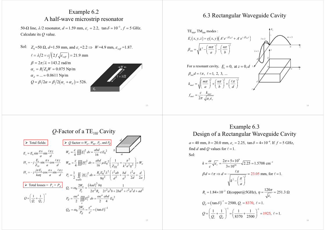
Example 6.2A half-wave microstrip resonatorA half wave microstrip resonator

350-Ω line, /2 resonator, 1.59 mm, 2.2, tan 10 , 5 GHz.rd f Calculate its value.

l

Q

0 =50 Ω, =1.59 mm, and =2.2 =4.9 mm, =1.87.

2 2 21.9 mm

r reff

reff

Z d W

c f

Sol:

0

2 143.2 rad/m0.075 Np/m

reff

R Z W

0 0.075 Np/m... 0.0611 Np/m

2 2 526.

c

d

d

R Z W

Q

2 2 526.c dQ

13

6.3 Rectangular Waveguide Cavity

TEmn, TMmn modes :

2 2

, , , mn mnj z j ztE x y z e x y A e A e

mn, mn

2 22

mnm nka b

0, at 0,tE z d For a resonant cavity,

2 2 2

, 1, 2, 3, ...mnd

m nk

mn

mn

ka b dkcf

14

2mnr r

f

Q-Factor of a TE10l Cavity

Total fields: Q factor , , , and e m c dW W P P

0 sin sinyx zE E

a dE x z

2 20

24 16

1

eabdW E dv E

bd

0

0

sin cos

cos sin

xTE

E x zH jZ a dj E x zH j

22 20 2 2 2 2

2 2 2 22

14 16

1

m eTE

abdW H dv E WZ k a

R E ab bd a d

cos sinzH jka a d

2 02 2 2

3

12 2 28

2 1

sc t

walls

R E ab bd a dP H dsd ad a

kad bW

Total losses = P + P

11 1Q

0 2 2 3 3 2 3 3

2 2

2 12 2 2

ec

c s

kad bWQ

P R a b bd a d adabdP E d E

Total losses = Pc + Pd

c d

QQ Q

202 2 4d

vP E dv E

Q

10

2tane

dW

15

Q 0 tanddP

Example 6.3Design of a Rectangular Waveguide CavityDesign of a Rectangular Waveguide Cavity

440 mm, 20.0 mm, 2.25, tan 4 10 . If 5 GHz, fi d d l f

ra b fd

92 5 10

find and values for 1.Sol:

d Q

91

10

2 5 10 2.25 1.5708 cm3 10

f 123 05

rkc

d d

22

mm, for 1.23.05d d

ka

2 1201.84 10 Ω(copper@5GHz), 251.3 Ωsr

R

1

1 1

tan 2500, , 1.

1 1 1 1

8370r

d cQ Q

16

1 1 1 1 , 1.8370 2500

1925c d

QQ Q

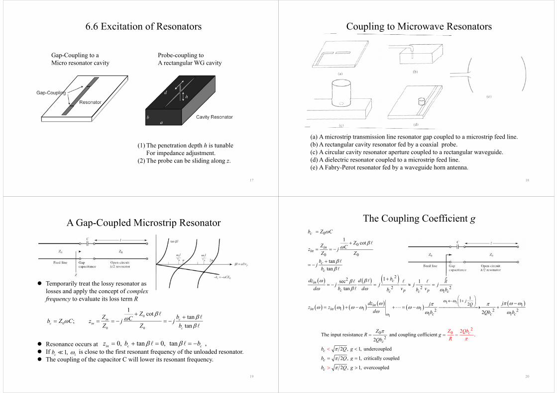
6.6 Excitation of Resonators

Gap Coupling to a Probe coupling toGap-Coupling to a Micro resonator cavity

Probe-coupling toA rectangular WG cavity

(1) The penetration depth h is tunable For impedance adjustment.

(2) The probe can be sliding along z.

17

( ) p g g

Coupling to Microwave Resonators

(a) A microstrip transmission line resonator gap coupled to a microstrip feed line. (b) A rectangular cavity resonator fed by a coaxial probe. (c) A circular cavity resonator aperture coupled to a rectangular waveguide. (d) A dielectric resonator coupled to a microstrip feed line.

18

( ) p p(e) A Fabry-Perot resonator fed by a waveguide horn antenna.

A Gap-Coupled Microstrip Resonator

Temporarily treat the lossy resonator as losses and apply the concept of complex frequency to evaluate its loss term R

01 cot tanZZ bC

0

00 0

tan;

tanin c

c inc

Z bCb Z C z j jZ Z b

Resonance occurs at If is close to the first resonant frequency of the unloaded resonator. The coupling of the capacitor C will lower its resonant frequency

0, tan 0, tan ,in c cz b b 11, cb

The coupling of the capacitor C will lower its resonant frequency.

19

The Coupling Coefficient gb Z C0

0

1 cot

c

inin

b Z C

ZZ Cz jZ Z

0 0tan

tan

in

c

c

jZ Z

bj

b

22

2 2 21

1sec 1tan

cin

c p pc c c

bdz dj j j j

d b d v vb b b

1 1

1

112 1

1 1 1 2 2 21 12

jQin

in inc c c

dz jjz zd b Qb b

1

02

20 The input resistance and coupling cofficient .

2 cZ QZR g

b Rb

22

2 , 1, undercoupled

2 1 critically coupled

c

c

c

Qb

b Q g

b Q g

R

20

2 , 1, critically coupled

2 , 1, overcoupledc

c

b Q g

b Q g

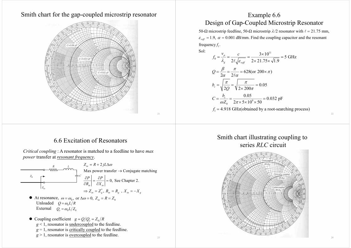
Smith chart for the gap-coupled microstrip resonator

21

Example 6.6D i f G C l d Mi t i R tDesign of Gap-Coupled Microstrip Resonator

50-Ω microstrip feedline, 50-Ω microstrip /2 resonator with 21.75 mm,

1

1.9, 0.001 dB/mm. Find the coupling capacitor and the resonant

frequency .reff

f

Sol: 11

03 10 5 GHz

2 2 21.75 1.9p

g ff

v cf

2 2 21.75 1.9

628(or 200 )2 2

g reff

Q

2 2

0.052 2 200cbQ

90

2 2 2000.05 0.032 pF

2 5 10 50c

QbCZ

22

0

1

2 5 10 504.918 GHz(obtained by a root-searching process)

Zf

6.6 Excitation of ResonatorsCritical coupling : A resonator is matched to a feedline to have max power transfer at resonant frequency.

2Max power transfer Conjugate matching

inZ R jL

p f q y

p j g g

0, See Chapter 2.in in

P PR X

At resonance,

* , , in in

in g in g in gZ Z R R X X

0 0, or 0, inZ R Z ,UnloadedExternal

0Q L R

0 0eQ L Z

0 0, , in

Coupling coefficient g < 1, resonator is undercoupled to the feedline.

0eg Q Q Z R

g = 1, resonator is critically coupled to the feedline.g > 1, resonator is overcoupled to the feedline.

23

Smith chart illustrating coupling to series RLC circuitseries RLC circuit

24

g X w y V Ñ I gx XÇw Éy VtÑA I

25

Time-Domain Analysis of Open CavitiesPart II

Time Domain Analysis of Open CavitiesLecture Notes and Computational Exercises＊

ffor Graduate Course "Microwave Physics and Applications"

Department of Physics, National Tsing Hua University, Hsinchu, Taiwan, R.O.C. and

Graduate Research and Training in Advanced Microwave and MM Wave Thermionics

University of California, Los Angeles, California, U.S.A.

*Developed under the Agreement on Academic Exchange and. Cooperation between Center for High Frequency Electronics (The University of California] Los Angeles) and High Frequency Electrodynamics Laboratory (National Tsing Huag ) g q y y y ( gUniversity)

The PowerPoint file is based on Prof K R Chu’s lecture notes

26

The PowerPoint file is based on Prof. K. R. Chu s lecture notes –Time-Domain Analysis of Open Cavities.

Time-Domain Analysis of Open Cavities

1. Introduction

2. Formulation

3. Numerical Algorithmg

4. A Fortran Exercise

i i5. Discussion

6. Appendix• Dispersion relation for a lossy waveguide• Complex-root finding by Muller’s method (Fortran)

I i f diff i l i i R K (F )• Integration of differential equation using Runge-Kutta (Fortran)• Spectral domain analysis of open cavity• Solution to exercise

27

• Solution to exercise

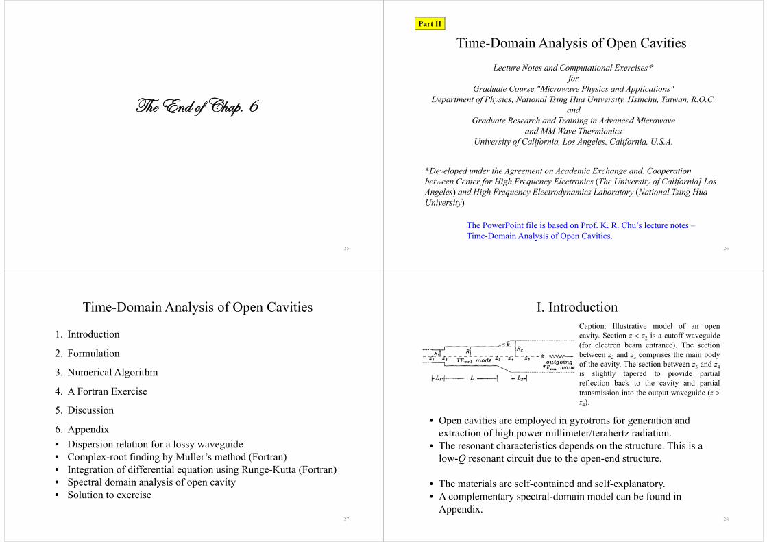
I. IntroductionCaption: Illustrative model of an opencavity. Section z z2 is a cutoff waveguide(for electron beam entrance). The section(for electron beam entrance). The sectionbetween z2 and z3 comprises the main bodyof the cavity. The section between z3 and z4is slightly tapered to provide partialg y p p preflection back to the cavity and partialtransmission into the output waveguide (z z4).

• Open cavities are employed in gyrotrons for generation and extraction of high power millimeter/terahertz radiation.extraction of high power millimeter/terahertz radiation.

• The resonant characteristics depends on the structure. This is a low-Q resonant circuit due to the open-end structure.

• The materials are self-contained and self-explanatory.• A complementary spectral domain model can be found in

28

• A complementary spectral-domain model can be found in Appendix.

II. FormulationConsider a typical open cavityformed of multiple sections ofuniform and linearly tapereduniform and linearly taperedstructures. Find the field profileand the Q-factor.

3 assumptions:• The waveguide radius changes slowly and there is no mode

d e Q c o .

e wavegu de ad us c a ges s ow y a d t e e s o odeconversion.

• A resonant mode is initially present in the cavity. All fields vary with time as exp(-iωt).

• The end sections are uniform to ensure the correctness of calculationcalculation.

(where < 0.)r i ii

29

( )r i i

Time-Domain Analysis

zThe time dependence of a field component (say ) is B

z ~ i rt i ti tB e e e

2 2Field energy ~ ~ , ( <0)itz iB e

Power loss ~ (field energy) = 2 (field energy)iddt

Q lit f t f th it

dt

Quality factor of the cavity:

field energyr rQ

30

power loss 2 i

Q

Characteristics of TEmn modeFor a circular waveguide with slowly varying radius rw(z) , the TE mode wave equation is expressed in a cylindrical coordinate system as,

( ) ( ) im i tm mnzB f z J k z r e

Applying the boundary condition on the side wall,

0 ( ) mnxB k( ) 0 ( ) ,

( )where is the -th root of ( ) 0

wmn

mnw

mn m

r r zzB k zr r z

x n J x

where is the th root of ( ) 0mn mx n J xSubstituting to the wave equation, we obtain

22 x 22 22

22 2 2

( ) above cutoff( )

( ) ( ) 0, where

mnz

wz

xk zc r zd k z f z

d

31

2 2 22

2 2( ) below cutoff( )mn

zw

dz xzr z c

Field Profile , if

( ) , where if

z z

z z

ik z ik zr cmn mn

cmnz z w

Ae Be cf zrCe De

The complex function of f(z) takes the general form,( )( ) ( ) i zf f

, if wr cmnCe De

The dependences of f(z) and Φ(z) on z indicate the nature of the

( )( ) ( ) i zf z f z e

wave.

• For a pure traveling wave (A = 0 or B = 0) |f(z)| is independent of z• For a pure traveling wave (A = 0 or B = 0), |f(z)| is independent of z, but Φ(z) is a linear function of z.

• For a pure standing wave (A = ± B), |f(z)| is a sinusoidal function p g ( ), |f( )|of z.

• For decaying waves at both ends, Φ(z) is independent of z.

32Use the boundary conditions to determine |f(z)| and Φ(z).

Boundary ConditionsOut-going wave boundary conditions: Initially there is a field profile satisfying all the boundary conditions and then decaying p y g y y gwith time.

A b h d A D 0 d C B 0At both ends, A=D=0 at z=z1 and C=B=0 at z5.

1 1 1( ) ( ) if ( )ik z f z z 1 1 11

1 1 1

( ) ( ), if ( )( )

( ) ( ), if ( )z r cmn

z r cmn

ik z f z zf z

z f z z

5 5 55

( ) ( ), if ( )( )

( ) ( ) if ( )z r cmnik z f z z

f zz f z z

5 5 5( ) ( ), if ( )z r cmnz f z z

33

Numerical Procedure

With a proper guess of the value of ωr and Q (ω= ωr +iωi).

f is given at z=z1 and f ′ is set accordingly.

Integrate from z1 to z5 using Runge Kutta method

Check the boundary condition at z and using Muller’s method Check the boundary condition at z5 and using Muller s method to guess the next root of ωr and Q.

Iterative integration, each time with an improved guess for ω, will eventually converge to a correct solution for ω, and f(z)

ill ti f ll th b d ditiwill satisfy all the boundary conditions.

34

Complex Boundary Condition (cbc sub-rountine)

Boundary condition at z=z1 is given. However the boundary condition at z=z5 needs to be checkedcondition at z z5 needs to be checked.

5 5 55

( ) ( ), if ( )( ) z r cmnik z f z z

f z

5 5 5

55 5 5

5

( )( ) ( ), if ( )

( ) ( ) ( ) if ( )cmz r n

f z ik z f z z

f zz f zz

5 5 5 5

5 5 5 5o

( ) ( ) ( ), if ( )( )

( ) ( ) ( ),

if ( )r z r cmn

z r cmn

f z ik z f z zD

f z z f zz

Standard root-finding algorithms such as Muller’s method can be readily used.

There are a series of discrete solutions for ω corresponding to different axial modes (assuming that the transverse mode number

35

( gm and n are given).

Comments

It is clear that the solution for should be independent of thepositions of z and z as long as they are in the uniform endpositions of z1 and z5 as long as they are in the uniform endsections.

Validity of the evanescent wave boundary condition requiresthat the end waveguide radius (Rl or R2) be smaller than the

it di (R)cavity radius (R).

It should also be noted that the assumption of slowly varyingp y y gcross-section is violated at z=z2 (Fig.1). This is justifiable onlyif the left end waveguide (z z2) is cutoff to the cavity mode. Inhi l fl i f h l f d k l jthis case, total reflection from the left end takes place just as a

more exact model would predict.

36

III. Numerical AlgorithmHow to integrate a differential equation?

222

2 2( ) above cutoffmnz

xk z

2 222

2 2 22

( ) above cutoff( )

( ) ( ) 0, where

( ) below cutoff

zw

zmn

k zc r zd k z f z

dz xz

The Runge-Kutta method:

The second order equation shown above can be decomposed into

2 2( ) below cutoff( )

zw

zr z c

the form of coupled real differential equations of the first order.

r if f if r rd f fdz

2 2 2R ( ) I ( )

r i

r i

f f ff f if

k k i k

i i

dzd f fdz

2 2 2Re( ) Im( ) z z z

ziz zr

k k i kkk k

i

2 2Re( ) Im( )z r z ird f k f k fdz

37

ziz zri

2 2Im( ) Re( )i z r z i

d f k f k fdz

III. Numerical AlgorithmInitial Boundary conditions at zInitial Boundary conditions at z1

The boundary conditions at z = z1 can be written,

1

1

( ) arbitrary real constant( ) arbitrary real constant

r

i

f zf z

1 1 1 1 11

1 1 1 1 1

( ) ( ) ( ) ( ), if ( )( )

( ) ( ) ( ) ( ), if ( )zr i zi r r cmn

rzr r zi i r cmn

k z f z k z f z zf z

z f z z f z z

1 1 1 1 1

1 1 11

( ) ( ) ( ) ( ), if ( )

( ) ( ), if ( )( )

(

zr r zi i r cmn

zr r zi i r cmni

z f z z f z z

k f z k f z zf z

f

) ( ) if ( )f

1 (izi rf 1 1 1) ( ), if ( )zr i r cmnz f z z

38

III. Numerical AlgorithmFinal Boundary Conditions at zFinal Boundary Conditions at z5

A guessed value for ω can now be integrated from zl to z5.

The resulting functions f (z5) fi(z5) f '(z5) and fi'(z5) give f(z5) The resulting functions fr(z5), fi(z5), fr (z5) and fi (z5) give f(z5) and f'(z5).

The procedure is to be repeated with an improved guess of until the required accuracy is achieved.

39

IV. A Fortran Exercise

The program (named CAVITY.f) consists of a main program and the following subprograms. 1 G l b1. General purpose subprograms.

MULLER: finding the complex roots of an arbitrary complex function (see Appendix B). RKINT f i i t ti f i lt diff ti l ti f th fi tRKINT: performing integration of simultaneous differential equations of the first order by the Runge-Kutta method (see Appendix C). SSCALE and SPLOT (or BSCALE and BPLOT): plotting data conveniently in characters (see Appendix D)characters (see Appendix D).

2. Subprograms written for CAVITY (It is recommended to go over the contents closely). CBC: evaluating the function D( ) in Eq (19) by integrating Eqs (24)-(27) withCBC: evaluating the function D( ) in Eq. (19) by integrating Eqs. (24) (27) with initial values given by Eqs. (28)-(31). DIFEQ: evaluating the derivatives in Eqs. (24)-(27). RADIUS: evaluating the cavity wall radius as a function of z.RADIUS: evaluating the cavity wall radius as a function of z. RHO: evaluating the wall resistivity as a function of z. CLOSS: evaluating the wall loss factor derived in Appendix E (The loss factor has been incorporated into the formalism in Appendix F.)

40

p pp )

Procedures for Running Program Cavity.f To begin, the cavity dimensions , mode of interest, and

numerical instructions, etc. are specified in the main program.

A guessed value of is then input into MULLER which calls CBC to evaluate D(ω). Subprogram CBC calls RKINT to perform the integration from zl to z5. Subsequently, RKINT calls DIFEQ to evaluate the derivatives at every z-step of the integrationintegration.

Finally, MULLER returns the solution for to the main program hi h i t ll th i f ti f i t t d ll SSCALEwhich prints all the information of interest and calls SSCALE

and SPOLT (or BSCALE and BPLOT) to plot and .

C bl k t i l l d f i f ti Common blocks are extensively employed for information sharing (e.g. the cavity dimensions specified in the main program and the field profile calculated in subprogram CBC)

41

program and the field profile calculated in subprogram CBC) between the main program and subprograms.

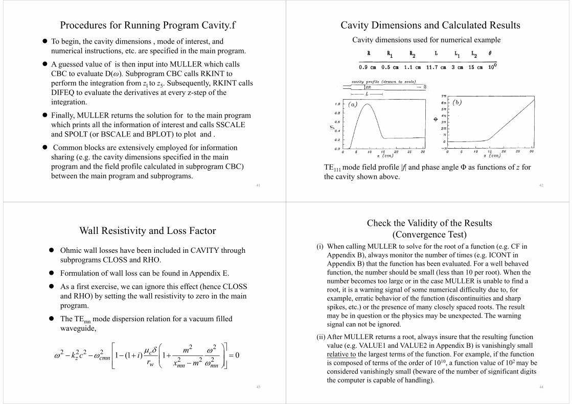
Cavity Dimensions and Calculated Results Cavity dimensions used for numerical example

TE mode field profile |f| and phase angle Φ as functions of z for

42

TE111 mode field profile |f| and phase angle Φ as functions of z for the cavity shown above.

Wall Resistivity and Loss Factor

Ohmic wall losses have been included in CAVITY through subprograms CLOSS and RHOsubprograms CLOSS and RHO.

Formulation of wall loss can be found in Appendix E.

As a first exercise, we can ignore this effect (hence CLOSS and RHO) by setting the wall resistivity to zero in the main program.

The TEmn mode dispersion relation for a vacuum filled waveguide,

2 2 2 22 2 2 2

2 2 21 (1 ) 1 0cz cmn

w mn mn

mk c ir x m

43

Check the Validity of the Results(Convergence Test)(Convergence Test)

(i) When calling MULLER to solve for the root of a function (e.g. CF in Appendix B), always monitor the number of times (e.g. ICONT in pp ) y ( gAppendix B) that the function has been evaluated. For a well behaved function, the number should be small (less than 10 per root). When the number becomes too large or in the case MULLER is unable to find anumber becomes too large or in the case MULLER is unable to find a root, it is a warning signal of some numerical difficulty due to, for example, erratic behavior of the function (discontinuities and sharp spikes, etc.) or the presence of many closely spaced roots. The result may be in question or the physics may be unexpected. The warning signal can not be ignoredsignal can not be ignored.

(ii) After MULLER returns a root, always insure that the resulting function value (e.g. VALUE1 and VALUE2 in Appendix B) is vanishingly smallvalue (e.g. VALUE1 and VALUE2 in Appendix B) is vanishingly small relative to the largest terms of the function. For example, if the function is composed of terms of the order of 1010, a function value of 102 may be

id d i hi l ll (b f th b f i ifi t di it

44

considered vanishingly small (beware of the number of significant digits the computer is capable of handling).

Check the Validity of the Results IICheck the Validity of the Results II(iii) A valid root is not necessarily the desired root. For example,

we provide a guessed value for the l=2 root and call MULLER to search around it for the correct =2 root. MULLER will return a different root (e g l=1 or 3) if theMULLER will return a different root (e.g. l=1 or 3) if the guessed value happens to be a better guess for that root. A reliable way to verify the l number of the root returned by y y yMULLER is to count the number of peaks in the versus z.

(i ) i h ll h h k h i ill h h(iv) Even with all these checks, there is still no guarantee that the results are free from numerical errors. We must also check whether the step size in the z integration is sufficiently fine towhether the step size in the z-integration is sufficiently fine to insure convergence of results.

45

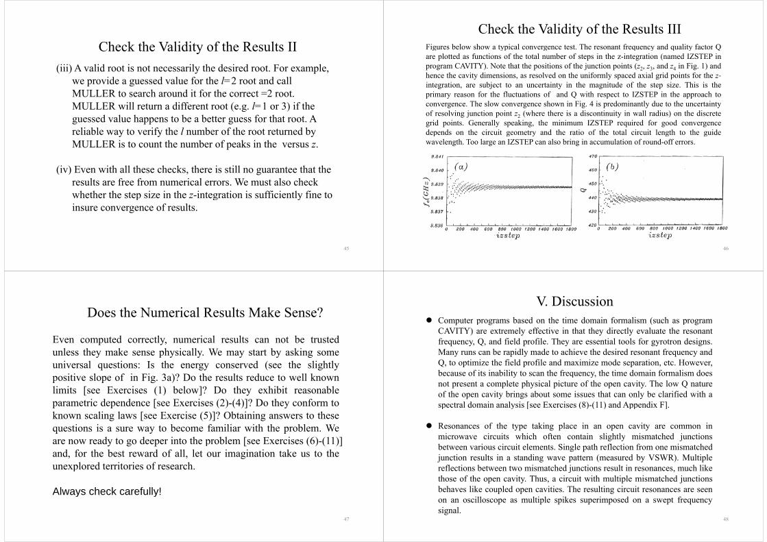
Check the Validity of the Results IIIFigures below show a typical convergence test The resonant frequency and quality factor QFigures below show a typical convergence test. The resonant frequency and quality factor Qare plotted as functions of the total number of steps in the z-integration (named IZSTEP inprogram CAVITY). Note that the positions of the junction points (z2, z3, and z4 in Fig. 1) andhence the cavity dimensions as resolved on the uniformly spaced axial grid points for the z-hence the cavity dimensions, as resolved on the uniformly spaced axial grid points for the zintegration, are subject to an uncertainty in the magnitude of the step size. This is theprimary reason for the fluctuations of and Q with respect to IZSTEP in the approach toconvergence. The slow convergence shown in Fig. 4 is predominantly due to the uncertaintyconvergence. The slow convergence shown in Fig. 4 is predominantly due to the uncertaintyof resolving junction point z2 (where there is a discontinuity in wall radius) on the discretegrid points. Generally speaking, the minimum IZSTEP required for good convergencedepends on the circuit geometry and the ratio of the total circuit length to the guidep g y g gwavelength. Too large an IZSTEP can also bring in accumulation of round-off errors.

46

Does the Numerical Results Make Sense?

Even computed correctly, numerical results can not be trustedunless they make sense physically. We may start by asking someuniversal questions: Is the energy conserved (see the slightlypositive slope of in Fig 3a)? Do the results reduce to well knownpositive slope of in Fig. 3a)? Do the results reduce to well knownlimits [see Exercises (1) below]? Do they exhibit reasonableparametric dependence [see Exercises (2)-(4)]? Do they conform top p [ ( ) ( )] yknown scaling laws [see Exercise (5)]? Obtaining answers to thesequestions is a sure way to become familiar with the problem. Weare now ready to go deeper into the problem [see Exercises (6)-(11)]and, for the best reward of all, let our imagination take us to theunexplored territories of researchunexplored territories of research.

Always check carefully!

47

y y

V. Discussion C b d h i d i f li ( h Computer programs based on the time domain formalism (such as program

CAVITY) are extremely effective in that they directly evaluate the resonantfrequency, Q, and field profile. They are essential tools for gyrotron designs.Many runs can be rapidly made to achieve the desired resonant frequency andQ, to optimize the field profile and maximize mode separation, etc. However,because of its inability to scan the frequency, the time domain formalism doesy q y,not present a complete physical picture of the open cavity. The low Q natureof the open cavity brings about some issues that can only be clarified with aspectral domain analysis [see Exercises (8)-(11) and Appendix F]spectral domain analysis [see Exercises (8) (11) and Appendix F].

Resonances of the type taking place in an open cavity are common inmicrowave circuits which often contain slightly mismatched junctionsmicrowave circuits which often contain slightly mismatched junctionsbetween various circuit elements. Single path reflection from one mismatchedjunction results in a standing wave pattern (measured by VSWR). Multiple

fl ti b t t i t h d j ti lt i h likreflections between two mismatched junctions result in resonances, much likethose of the open cavity. Thus, a circuit with multiple mismatched junctionsbehaves like coupled open cavities. The resulting circuit resonances are seen

48

on an oscilloscope as multiple spikes superimposed on a swept frequencysignal.

Exercise (1)1. For the open cavity of Fig. 1 with dimensions given in Table I,

the resonant frequency of the TE111 mode is 9.839 GHz (see Fig. 4) For an enclosed cylindrical cavity with the same radius (0 94). For an enclosed cylindrical cavity with the same radius (0.9 cm) and length (11.7 cm) as those of the main body of the open cavity, the resonant frequency of the TE111 mode is 9.851 GHz. y, q y 111Explain the difference qualitatively.

Sol: Because of the fringe field, the open cavity has an effective length longer than L, hence the resonant frequency (of the >0 modes) is lower than that of an enclosed cavity of length L It is

modes) is lower than that of an enclosed cavity of length L. It is worth noting that for the =0 (TM) modes of an enclosed cavity for which the axial field profile is uniform, an opening at either

p , p g

end will impose an axial mode structure and therefore increase the resonant frequency.

49

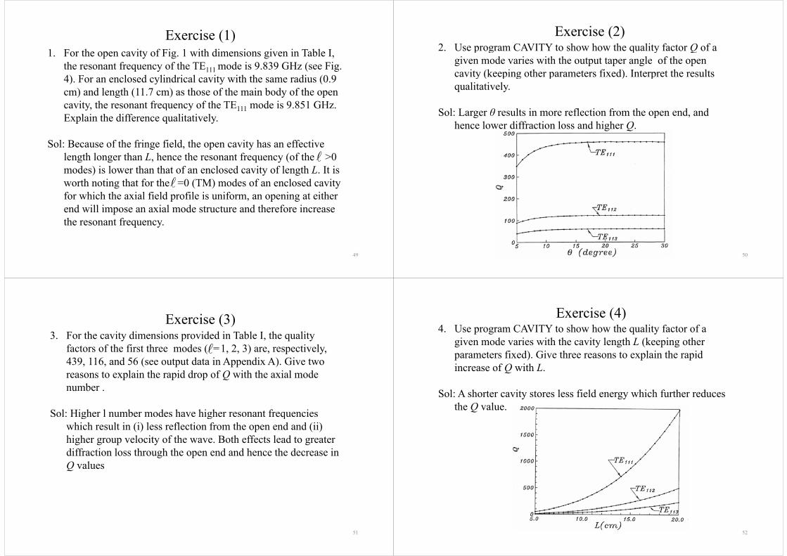
Exercise (2)2 Use program CAVITY to show how the quality factor Q of a2. Use program CAVITY to show how the quality factor Q of a

given mode varies with the output taper angle of the open cavity (keeping other parameters fixed). Interpret the results y ( p g p ) pqualitatively.

S l L θ l i fl i f h d dSol: Larger θ results in more reflection from the open end, and hence lower diffraction loss and higher Q.

50

Exercise (3)( )3. For the cavity dimensions provided in Table I, the quality

factors of the first three modes ( =1, 2, 3) are, respectively, 439, 116, and 56 (see output data in Appendix A). Give two reasons to explain the rapid drop of Q with the axial mode numbernumber .

Sol: Higher l number modes have higher resonant frequencies g g qwhich result in (i) less reflection from the open end and (ii) higher group velocity of the wave. Both effects lead to greater diffraction loss through the open end and hence the decrease in Q values

51

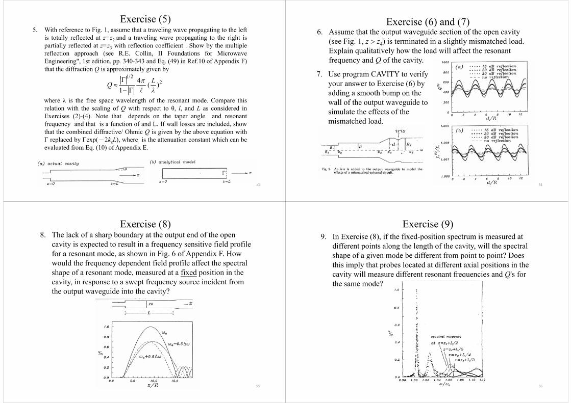
Exercise (4)4 U CAVITY t h h th lit f t f4. Use program CAVITY to show how the quality factor of a

given mode varies with the cavity length L (keeping other parameters fixed) Give three reasons to explain the rapidparameters fixed). Give three reasons to explain the rapid increase of Q with L.

Sol: A shorter cavity stores less field energy which further reduces the Q value.

52

Exercise (5)5. With reference to Fig. 1, assume that a traveling wave propagating to the left

is totally reflected at z=z2 and a traveling wave propagating to the right ispartially reflected at z=z3 with reflection coefficient . Show by the multiplereflection approach (see R.E. Collin, II Foundations for MicrowaveEngineering", 1st edition, pp. 340-343 and Eq. (49) in Ref.10 of Appendix F)that the diffraction Q is approximately given by

1/2 4 L

where λ is the free space wavelength of the resonant mode Compare this

24 ( )1

LQ

where λ is the free space wavelength of the resonant mode. Compare thisrelation with the scaling of Q with respect to θ, l, and L as considered inExercises (2)-(4). Note that depends on the taper angle and resonantfreq enc and that is a f nction of and L If all losses are incl ded shofrequency and that is a function of and L. If wall losses are included, showthat the combined diffractive/ Ohmic Q is given by the above equation with replaced by exp(－2kzL), where is the attenuation constant which can be

l d f ( ) f dievaluated from Eq. (10) of Appendix E.

53

Exercise (6) and (7)6. Assume that the output waveguide section of the open cavity p g p y

(see Fig. 1, z z4) is terminated in a slightly mismatched load. Explain qualitatively how the load will affect the resonant frequency and Q of the cavity.

7. Use program CAVITY to verify your answer to Exercise (6) by adding a smooth bump on the

ll f th t t id twall of the output waveguide to simulate the effects of the mismatched load.mismatched load.

54

Exercise (8)8 The lack of a sharp boundary at the output end of the open8. The lack of a sharp boundary at the output end of the open

cavity is expected to result in a frequency sensitive field profile for a resonant mode, as shown in Fig. 6 of Appendix F. How would the frequency dependent field profile affect the spectral shape of a resonant mode, measured at a fixed position in the

it i t t f i id t fcavity, in response to a swept frequency source incident from the output waveguide into the cavity?

55

Exercise (9)9 In Exercise (8) if the fixed position spectrum is measured at9. In Exercise (8), if the fixed-position spectrum is measured at

different points along the length of the cavity, will the spectral shape of a given mode be different from point to point? Does p g p pthis imply that probes located at different axial positions in the cavity will measure different resonant frequencies and Q's for the same mode?

56

Exercise (10)

10. Write a computer program based on the spectral domain formalism in Sec. II of Appendix F to: • verify your answers to Exercises (8) and (9) • calculate the reflection coefficient assumed in Exercise (5) as a function of

the wave frequency. q y• calculate the reflection coefficient at the smooth bump assumed in Exercise

(7) as a function of the wave frequency.

Sol: RFS or RFS2

57

Exercise (11)11 Program CAVITY calculates Q by its time domain definition (denoted by11. Program CAVITY calculates Q by its time domain definition (denoted by

superscript “t”)

While the spectral domain formalism yields Q by its spectral domain definition

(t)2

r

iQ

While the spectral domain formalism yields Q by its spectral domain definition (denoted by superscript “ω”)

h Δ i th FWHM b d idth C i l d ith

( )Q

where Δ ω is the FWHM bandwidth. Compare numerical runs made with program CAVITY with those made with the program developed in Exercise (10) to show that, for the same mode of a low Q open cavity, the two definitions of Qdo not yield the same result and

Explain this result qualitatively.

( ) ( )tQ Q

p q y( )2( , ) ( )j

j tj

i t tQ

jj

f t f e

x x

( )0

2 *

1 1( , ) ( , ) ( )22 2

1 1

i tj t

j j j j

if f t e dt fi Q

i i

x x x

58

2 *( ) ( )

( ) ( )

1 1( , ) ( ) ( )2 22 2

... Q

j jt tj jj j j j j j

t

i if f fi Q i Q

Q

x x x

Appendix: Muller’s Method

Note: Muller’s method is discussed in Conte and de boor, Elementary Numerical Analysis”, (3rd edition, Sec. 3.7).

59

y , ( , )

Appendix: Runge-Kutta’s Method (RKINT)

60

Appendix: Dispersion Relation for a Lossy WaveguideD i ti f th l f t i E (19) f A di FDerivation of the loss factor in Eq. (19) of Appendix F.

Jackson, Chap. 8

2 22 2 2 2 1 (1 ) 1 0c mk c i

2 2 21 (1 ) 1 0z cmn

w mn mnk c i

r x m

61

Spectral-Domain Analysis of Open CavitiesPart III

Reason: Cold tests of open cavities almost always employ the

method of frequency sweeping and Q is measured by its spectral

domain definition (hence denoted by superscript ω) where Δω is the ( y p p )

full width between the half maxima of the resonant line.

Q lit f t f th itQuality factor of the cavity: Time-domain definition:

fi ld( ) field energy power loss 2

t rr

iQ

( ) 0

Frequency-domain definition:

Q What is the difference

62

Q between these two definitions?

II. Numerical Approaches for the Spectral Model3 assumptions:• The waveguide radius changes slowly and there is no mode

conversion. • A resonant mode is initially present in the cavity. All fields vary

with time as exp( iωt)with time as exp(-iωt). • The end sections are uniform to ensure the correctness of

calculation.

Time-domain model:(where < 0 )i (where < 0.)r i ii

Frequency-domain model:?C l fl ti ffi i t

63

Complex reflection coefficientΓ

Numerical Model

1 1 1 1( ) ( )1( ) z zik z z ik z zf z e e

With a proper guess of the value of Γ (Γ = Γr +i Γi).

1 1 1 1

1( ) ( )

1

( )

( ) ( )z zik z z ik z zz

f z e e

f z ik e e

where r cmn

f is given at z=z1 and f ′ is set accordingly.

Integrate from z1 to z5 using Runge-Kutta method

Check the boundary condition at z and using Muller’s method Check the boundary condition at z5 and using Muller s method to guess the next root of Γ.

Iterative integration, each time with an improved guess for ω, will eventually converge to a correct solution for ω, and f(z) will satisf all the bo ndar conditions

64

satisfy all the boundary conditions.

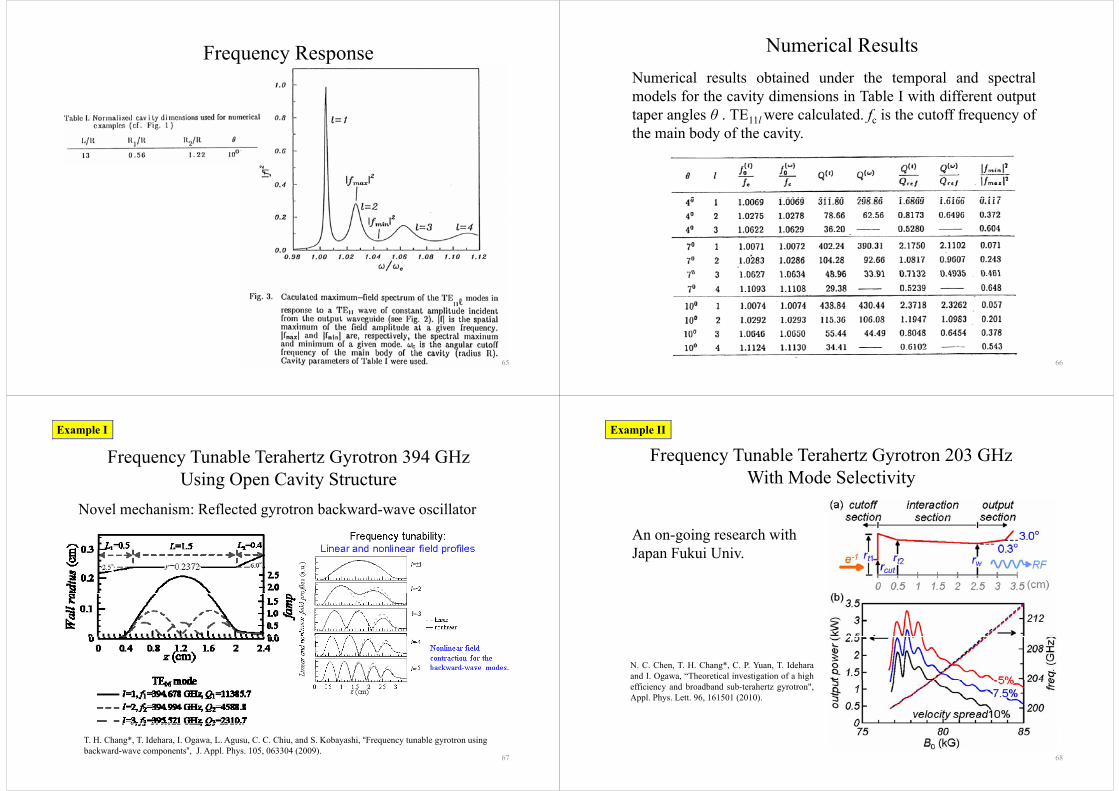
Frequency Response

65

Numerical ResultsNumerical results obtained under the temporal and spectralmodels for the cavity dimensions in Table I with different outputt l θ TE l l t d f i th t ff f ftaper angles θ . TE11l were calculated. fc is the cutoff frequency ofthe main body of the cavity.

66

Frequency Tunable Terahertz Gyrotron 394 GHzExample I

q y yUsing Open Cavity Structure

N l h i R fl t d t b k d ill tNovel mechanism: Reflected gyrotron backward-wave oscillator

67

T. H. Chang*, T. Idehara, I. Ogawa, L. Agusu, C. C. Chiu, and S. Kobayashi, “Frequency tunable gyrotron using backward-wave components”, J. Appl. Phys. 105, 063304 (2009).

Frequency Tunable Terahertz Gyrotron 203 GHzExample II

q y yWith Mode Selectivity

An on-going research with J F k i U iJapan Fukui Univ.

N. C. Chen, T. H. Chang*, C. P. Yuan, T. Ideharaand I. Ogawa, “Theoretical investigation of a highg , g gefficiency and broadband sub-terahertz gyrotron",Appl. Phys. Lett. 96, 161501 (2010).

68

g X w y bÑ V |à gx XÇw Éy bÑxÇ Vtä|àç

69