Chebyshev spectral approximation of Navier …...HMW IMOâJSATMW MATHÉMATIQUE ET ANALYSE HUNÉftKKIE (Vol 21, n 1, 1987, p 93 à 123) CHEBYSHEV SPECTRAL APPROXIMATION OF NAVIER-STOKES

RAIROMODÉLISATION MATHÉMATIQUE

ET ANALYSE NUMÉRIQUE

Y. MADAY

B. MÉTIVETChebyshev spectral approximation of Navier-Stokesequations in a two dimensional domainRAIRO – Modélisation mathématique et analyse numérique,tome 21, no 1 (1987), p. 93-123.<http://www.numdam.org/item?id=M2AN_1987__21_1_93_0>

© AFCET, 1987, tous droits réservés.

L’accès aux archives de la revue « RAIRO – Modélisation mathématique etanalyse numérique » implique l’accord avec les conditions générales d’uti-lisation (http://www.numdam.org/legal.php). Toute utilisation commerciale ouimpression systématique est constitutive d’une infraction pénale. Toute copieou impression de ce fichier doit contenir la présente mention de copyright.

Article numérisé dans le cadre du programmeNumérisation de documents anciens mathématiques

http://www.numdam.org/

http://www.numdam.org/item?id=M2AN_1987__21_1_93_0

http://www.numdam.org/legal.php



H M W IMOâJSATMW MATHÉMATIQUE ET ANALYSE HUNÉftKKIE

(Vol 21, n° 1, 1987, p 93 à 123)

CHEBYSHEV SPECTRAL APPROXIMATIONOF NAVIER-STOKES EQUATIONS

IN A TWO DIMENSIONAL DOMAIN (*)

by Y. MADAY (*), B. MÉTIVET (2)

Communiqué par R TEMAM

Résumé — On analyse dans cet article l'estimation de l'erreur commise dans l'approximationpseudo-spectrale de la solution des équations de Navier-Stokes homogènes posées sur un carré Laformulation en fonction de courant de ces équations a été choisie pour plusieurs raisons détailléesdans l'introduction Les résultats de convergence sont optimaux c'est-a-dire du même ordre que lameilleure approximation polynômiale

Abstract — We analyse hère the convergence of a pseudo-spectral method for the approximationofthe homogeneous Navier-Stokes équations over a square We use the stream function formulationjor vanous reasons detailed in the introduction We prove optimal convergence rate i e oj the sameorder as the best polynomial approximation

I. INTRODUCTION

We present and analyse hère a Chebyshev spectral method for non periodic,steady-state, 2-D incompressible Navier-Stokes équations.

A very large littérature exists now concerning the numerical resolution ofNavier-Stokes équations by spectral methods (see Voigt-Gottlieb-Hussaini[1] for a survey).

Generally the velocity pressure formulation of the équations is used

duy= — v Aw + u. Vw + V/7 = ƒ in the domain,

" (1.0)div u = 0 in the domain

with often periodic boundary conditions in 1, 2 or 3 directions.

C) Université de Pans XII, Laboratoire d'Analyse Numérique de l'Université P et M Cime,Tour 55/65,5e Et, 4, Place Jussieu, 75252 Pans Cedex 05 (France) et Consultant ONERA

(2) Travail effectué à l'ONERA, 29, Avenue de la Division Leclerc 92320 Châtillon (France).Adresse actuelle EDF/DER/IMA/MMN, 1, Avenue du Général de Gaulle, 92141 Clamart(France)

M2 AN Modélisation mathématique et Analyse numérique 0399-0516/87/01/93/31/S 5 10Mathematical Modelhng and Numerical Analysis © Ah CET Gauthier- Villars

9 4 Y. MADAY, B. MÉTIVET

The great problem with non periodic boundary conditions is the treatmentof the pressure. In order to solve numerically (1.0), the varions authors proposedifferent stratégies for handling separately the velocity and the pressure :

* The most obvious way to obtain an équation for pressure is to take thedivergence of the équation of momentum to obtain the following Poissonéquation :

Ap = div ƒ — div (w. Vw).

Various boundary conditions can be imposedthen : Orszag-Israeli-Deville [1]have analysed several boundary conditions on pressure. Their conclusion isthat numerical instabilities lead to prefer conditions with no physical meaning.These methods are compared in Deville-Kleiser-Montigny [1].

The best suited type of boundary conditions is :

div u = 0 .

It has been used by Kleiser-Schumann [1] and Lequeré-Alziary de Roque-fort [1] but requires the inversion of the so called influence-matrix which islarge, full and ill-conditioned. This method is then difficult to use in 3-D nonperiodic situations.

* Another strategy, that can be used in 3-D non periodic curved domainsis proposed by Métivet-Morchoisne [1] (see also Métivet [1]). It consists in anitérative method based on a minimization of divergence at each time step thatdoes not involve boundary conditions over the pressure, this one being consi-dered as a Lagrangien multiplicator. A method with no boundary conditionsover the pressure is also proposed in Malik-Zang and Hussaini [1] for a 2-Dperiodic/non periodic problem.

* A last treatment consists in the élimination of the pressure. A clever choiceof divergence free velocity expansion functions can be used then, if directions ofperiodicity exist (see Mozer-Moin-Leonard [1]). But it seems difficult to begeneralized to pure non periodic boundary conditions.

In fact, the difficulty encountered hère, due the compatibility conditionsbetween velocity and pressure, is well known in finite element method and liespartially in a good choice for velocity and pressure discrete spaces. This condi-tion is known as " inf-sup condition" (see Girault-Raviart [1]). This problem,in spectral framework, has been analised in Bernardi-Maday-Métivet [2].

However, there exist two other présentations of 2-D incompressible Navier-Stokes équations that do not involve such a problem : the stream function-vorticity formulation that requires boundary conditions on vorticity, and

M2 AN Modélisation mathématique et Analyse numériqueMathematical Modelling and Numerical Analysis

NAVIER-STOKES EQUATIONS 95

the stream function formulation. The last one has been used for numerical reso-lution in Morchoisne [1] and its extension to 3-D case is studied

In this paper we analyse the 2-D approximation of this formulation :Find Y, defined over Q = ] - 1, 1[2, such that :

A 2\Xi if A lT/\ 1 I / A Vf/\ I y ï ^+ ^ - ^ ; - ^ r â ^ r 'm ' (ii)4* = S^ = O over T = ôfi.

Note that problem (1.1) is well fitted to spectral approximations since theiraccuracy increases with the regularity of the function Ç¥ is more regular than u).We prove here that the coUocation method leads to a discrete solution *¥N

asymptotically as close to *F as the best polynomial approximation of *F.For other theoretical analysis concerning spectral approximations of Navier-

Stokes équations we refer to Maday-Quarteroni [1], Bernardi-Maday-Métivet[1], [2] and Bernardi-Canuto-Maday [1] for pure spectral methods and Canuto-Maday-Quarteroni [1] for a combined finite element and spectral method.

In section 2 we recall some theoretical results concerning the approximationby Chebyshev spectral methods.

In section 3 we consider the approximation of the Stokes problem and sec-tion 4 deals with the Navier-Stokes problem. Optimal error bounds are provedThe analysis is based on the use of results of Descloux-Rappaz [1] on theapproximation of branches of non singular solution of P.D.E.. We indicate inthe appendix a suitable version of their theorems 3.1,3.2.

Acknowledgements : The authors wish to express their gratitude to ProfessorA. Quarteroni for a detailed criticism of an earlier version of this paper andDoctor Y. Morchoisne for valuable discussions.

IL NOTATIONS AND DEFINITIONS

Let / = ]— 1, -f 1[ and Q = I x /. A point of / (resp. Q) is denoted byx(resp. x = (xl9 x2))andF = dQ.

Let O e 9 '(Q); then D" <S> means 2 d> for any a = (al5 a2) in N2,ÖX-^ OX2

and I a I = 04 + a2.We consider the weight function (o(x) = (1 - x2)~1/2, xe I, associated with

the Chebyshev polynomials, and œ(x) = ©(xj œ(x2), x e Q. We define the

vol. 21, n° 1, 1987

9 6 Y. MADAY, B. MÉTIVET

weighted Sobolev spaces H^(Q) as follows :

(i) /Ç(Q) = L^(Q) = { O : Q -> U | d> is measurable and (O, *) 0 > a < oo },

=

(ii) for any

These spaces are Hilbert spaces for the scalar product :

((*,x)),.«= E (öa*,öBx)O i . .||

(iii) for any 5 e R + \ N , /Ç(Q) is defined by interpolation of index 5 - 1between H^(Q) and H^+1(iï) where 1 is the greatest integer ^ s (see Bergh-Löfström [1] for the définition of interpolation).

The norm of H^(iï) will be denoted by ||. ||SiS in the sequel. For any seU +

we dénote by H^JQ) the closure of 9 (il) in //£(Q). Let us recall that :

* For anyse[R + \ N u i N + - i , H^Jil) is the interpolate space of

l/2

, (2.1)

index s - J between HlJQ) and* For any s e N :

is a norm over HQ^Q) equivalent to the norm ||. ||s ^ (see Grisvard [1] for moredetails).

If X and Y are two Banach spaces such as X c: Y then X ^^Y (resp.X <-> 7) will mean that the identity mapping is continuous (resp. compact)from X into 7. We recall now some rather simple properties (see Maday [3]) :

H'Jfl) c^ C°(Q) for any s > 1 , (2.2)

Hs + 1/2(Q) c_ /^(Q) for any O O , (2.3)

iî/^(Q) is an algebra for any s > 1 . (2.4)

Next we introducé some notations and results commonly used in spectralmethods. Let PN(I) (resp. Q\(Q)) dénote the space of all polynomials overR of degree ^ N (resp. over U2 of degree ^ JV in each variable).



The results we will mention now are valid for 0 = / or 0 = Q, the variousnorm ||. ||SfCB and scalar product (.,.)o,« standing for the one previously definedif 0 = Q, and for those defined m the same way for 8 = /.

For any (p, v) e R2, 0 ^ ju ^ v, there exists a positive constant C such that :(inverse inequality)

II * llv.. < CN2*"* || O | | ^ , VO e Pê ) , (2.5)

Besides, let n0 J V dénote the orthogonal projection operator from L2(0) ontoPN(Q\ we have :

|| O - nO)JV<I> ||Oftt ^ CN-° | | * | | f f i . , V * e f Ç ( 6 ) , (2.6)

(see Canuto-Quarteroni [1] for the proofs of (2.5) and (2.6)). Let V = H§tJQ)and VN = V n PN(9). We recall that, for any real r ^ 2, there exists an operatorn rAf from Hffl) n F onto KN such that :

II * - nrsJV 0» ||Miœ «c CN»-" || < ||ViŒ , VO E H:(Q) n V ,

0 ^ p < r < v . (2.7)

(see Maday [1] and [3]).Let F%% = { &» CÜJ | 0 < i < AT}, (resp. F ^ = { ( ^ œtJ) | 0 < ij < AT }),

be the set of abcissae and weights of the Gauss Lobatto quadrature formulaof order 2JV - 1 associated with the weight CD (resp. co).

From the définition we have the following properties :

^ - = ( ^ y and ©„ = ©,©,, Oîj^N,

for any pair (<D, %) e C°(0)2 such that O % e P2JV-i(0) w e n a v e '•

(o(x) dx = (O, x)Op. , (2.8)

(here, the notation /(AT) stands for { 0, 1,..., N } if 0 = Iand for { 0, 1,..., JV } x{0, 1,..., JV } if 0 = Q, in this latter case i is an element of N 2).

Let us set :

( * , X ) . . N = E 0>(ÜX(U<fl,, V(<D,x)eC°(ë)2. (2.9)I(N)

This bilinear form is a scalar product over PJV(9). The associated norm isdenoted || . ||ujv, and vérifies the following property (see Canuto-Quartero-ni [1]) :

II * llo,« < II ® I U < 4 1| 0> ||OtB , V$ e PN(9) . (2.10)

vol 21, n° 1, 1987

98 Y. MADAY, B. MÉTIVET

Let us now introducé the interpolation operator PN (resp. PN) at the point^ (resp. %h) defined by :

PN : C°(J) -> Pî ) (resp. : C°(S) - PW(

= <P(U , 0 ^ i < N (resp. £*(*) (Ç „) = O ( y ,

0Ûj<N). (2.11)

These operators verify : (we use again an unique notation for the one and twodimension cases)

ff |i <D iiO)(û, VO e J ^ ( 9 ) , (2.12)

with a > 1/2 if 0 = / and a _> 1 if 9 = O.Moreover, for any O e C°(0), x

C || X llo,.(ll <">-PN* llo.» + ll «"Ho,*-! O llo.J

(2.13)

(see Maday-Quarteroni [3]).

in. SOME RESULTS CONCERNING THE CONTINUOUS PROBLEM

Hl- L The biharmonic prohlem

Let us fïrst consider the following biharmonic problem :Given g, find T such that :

A2xF = g in Q

d¥ (3.1)¥ = 0 , ^ = 0 on 3Q .

In order to analyse a spectral approximation of that problem we want tofind a solution *F in V = HQJQ). A necessary condition for solving problem(3.1) is that g (being the laplacian of an element of L^) belongs to the spaceJ*?-2(Q) defined by :

= { /= Z D*ga,gaeL$n); OLEN2}. (3.2)

The main resuit of this section states that this condition is also sufïïcientLet us first recall a preliminary one-dimensional resuit which can be found

in Maday [1].

M2 AN Modélisation mathématique et Analyse numériqueMathematical Modelhng and Numencal Analysis


LEMMA 3 . 1 : There exist positive constants Ct and C2 such that, for anycp e Hlm(I),

f cp2 (o9 dx ^ Q f cp'2 co5 dx < C2 f cp"2 ca dx . (3.3)

Moreover there exist positive constants C[ and C2 such that, for any

cp(XO))" dx

f cp"((p©)" dx

(3.4)

(3.5)

These results will now be extended to the 2-D case.

LEMMA 3.2 : There exist two positive constants a and P such that, for any

[1

(3.6)

(3.7)

Proof: Let O and % be in @>(Q). Then, Oœ and %co belong also to ^(f i ) and wecan write :

1 x = A20 + 2AU + A02, (3.8)

where Ati = I DiiJ) Q>D(il\%(ù) dx .Ja

We have : (we précise here by O; the factor in © which dépends onxi,i=l, 2)

Using (3.4) we obtain :

co20,0)1

vol. 21,11° 1, 1987


so that, from the Cauchy-Schwarz's inequality we get :

I ^ 2 0 I < C { I I * « 2 * 1 1 X 1 1 2 * '

Similarly, we fmd :

\A02\^C[ | | O | | 2 ) J | x i l 2 , m .

and :

dxx dx2 Ojm co dxx dx2

(3.9)

(3.10)

(3.11)

ôco, ,Since r— = x, GO, we obtain :

dx.

co ôxx ôx2.4

),© l_ ôx1 ôx2

JNow using (3.3) we hnd :

ro dx! êx2 dxx dx2(3.12)

Thus, the estimate (3.6) follows from (3.8)-(3.12).Next, in order to dérive the ellipticity condition (3.7) we take % = <S> in (3.8).

Using (3.5) we have :

^ 2 0

and

AQ2

- 3 (ù1dx1)dx2

co2 dx2 ) dx± ^ C2

2

0,û>

(3.13)

M2 AN Modélisation mathématique et Analyse numériqueMathematical Modelling and Numencal Analysis

NAVŒR-STOKES EQUATIONS

Let us now check that the term Axlis nonnegative. We set :

101

J =

Since :

^ = *< G>,3 and œf

an elementary calculation shows that :

X O 2 co5co5

But we note that, for x e Q :

2 r2 4- ^ x2 4- ^ Y2

1 * 2 + 8 X l + 8 2 ~ 2

Since J is non négative we obtain :

X10.

Thus it foUows from (3.8) and (3.13) that :

i A(Oo)) dx > C2d2®dx\

d2®dx2

<Dœ3l oT 1

1 x, O«

(3.14)

(3.15)

(3.16)

For proving (3.7), it remains to check that there exists C' ^ 0 such that :

vol. 21, n° 1, 1987

102 Y. MADAY, B. MÉTTVET

In fact, integrating by parts yields :

hence, we have :

Using (3.14) we find :

d /5O \ d2® d®-= -z © i = —-=• COi +

hence we have :

\~l2 m . f r/^2a>\2

ro + 2

© .]*

Integrating by parts and using (3.14) once more we obtain :

-0+*î)|£-| «Ï^K- (3.19)

Similarly we find :

-dxl) -

(3.190


NAVŒR-STOKES EQUATIONS 103

We dérive the estimate (3.17) with C' = ^ from (3.18)<3.19'). The ellipticity

condition (3.7) follows from (3.16), (3.17) and the property (2.1). •Let us now consider an element g of H~ 2(Q) = (H^JQ))'. It follows from

lemma 3.2 and Lax-Milgram theorem that there exists a unique solution *Fof problem :

find VeV such that :

*CF,X) = < £ * > , V X e V , (3.20)

where aÇ¥, x) = | A¥A(xœ) dx and < .,. > stands for the /Ç2(Q) x H2JQ)

duality pairing.Taking % e &(Q) in (3.20) we deduce that the solution ¥ of (3.20) vérifies :

(A2¥) (Ù = g,

(this equality holds in @'(ÇÏ)). Hence, for any g in H~2(Q\ there exists a unique¥ of V such that

A2x¥ = -£, (3.21)

this equality holds in S) '(Q) and more precisely in J^^ 2(Q).

For any g e J t y 2(Q) we know that there exists ~(0«)|a| *^2> 9« e L^Q) such

that g = Z D* O*- This element can be associated with g of H^2(Q) as

follows (remind (3.4)) :

l«l 2 Jn

:, V O e F , (3.22)

gris independent of the décomposition g = ^ Da â. Indeed if there exist|a|<2

^; in L^(Q), ! a | ^ 2 such that :

a 0«= Z D 8 » ;|a|<2

this equality holding in &'(&) ; then, for any % in

Z f ( - i)Wg*D«xdx= Z f ( -

vol. 21, n° 1, 1987


this result remains true if we take % = <ï>a) with O e ^(Q) ; by density we thendérive that g is independent of the décomposition of g.

The previous remark and (3.21) prove that the mapping of @'(Q) :

u h

(0

defines an isomorphism from H^2(Q) onto ^fia"2(Q); hence, we can solve

problem (3.1) in V iff g e ^ ~ 2 ( Q ) . This enables us to define an operatorT: ge^2(Q)^TgeVby:

a ( T 0 , x ) = < & * > > V X G K . (3.23)

THEOREM 3 . 1 : The linear operator T is boundedfrom 3^~2(^ï) into V andis

a linear compact operator from H~S(Q) into V for any s such that 0 < s < -?.

Remark 3 . 1 : The space Jf?(ù~

2(Q) is now equipped with the norm :

II 9 ll*£2<n) = II 0 liff^tn)-

Proof : The first part of this theorem is an easy conséquence of Lax-Milgramtheorem.

Let g 6 H~S(Q). It follows from Grisvard [2] or more easily from Bernardi-Raugel [1] that there exists an ƒ in HA~ S(Q) n ifo

2(Q) such that :

à2f=9, (3.24)and

^s(Q)<C\\g\\H.sm. (3.25)

Hence T is continuous from H~S(Q) into H4~S(Q). It is well known (seeAdams [1]) that i/4~s(Q) ^H5I2(Q). From (2.3) we dérive that

T is then compact from H~S(Q) into H2(Q) and the theorem is proved.

III.2. The Navier-Stokes problem

Let B be defined by : for any (O, %) e


NAVIER-STOKES EQUATIONS

and, for any (X, O) G IR x ®(Q), ƒ e @f(Q) :

105

!>) -ƒ]• (3.27)

From the next lemma we see that, the Navier-Stokes équations (1.1) consistin fmding T e F such that :

(3.28)with

LEMMA 3 .3 : Let us assume that 1 < s < 3/2 ;i) There exists a constant y > 0 such that, for any (<D, %) ƒ«

II B{% x ) l i n - d û < Y II * II2,«> II X I k . • ( 3 . 2 9 )

ii) 5 ca« be extended in a continuons mapping from V2 into H~S(Q).

Proof : Let (<D, x, S) in ^(Q)3, from (3.26) we obtain :

fJn

dxlr ^ x ü ^ s rfx f fx 50 as rfx

Jo a*ï 3JC2 3*! - )adx\dx2dxl -

Jn dxi dxl dx2 - Jn dxl d*i ox2 -

JQô*î 3^0X2 - J o 3JC5 3jt! 3x2 -"

(3.30)

We shall only consider the first term ; the others can be treated in the same way.2

Let q = _ ; then, due to the hypothesis on s, we have 4 < q < oo. There-

fore, from Hölder's inequality we have :

dx<>dx

dZdx1

2q({q-2)dx

(q~2)f2q(3.31)

vol. 21, n° 1, 1987

106 Y. MADAY, B. MÉTTVET

Moreover it is well known that (see Adams [1]) :

3v «

ln

ÔE

dx

dxx

'A, 2

2qf(q-2)dx

(q-2)f2qCI! H

By (3.31) and the obvious imbedding tf^(Q) ^ H2(Q), we get :

dZC d2db d% dE

Jn dx\ dx2 dx, ~- Cil «II,

and (3.29) follows. The end of the lemma is derived by a classical densityargument. •

With the previous notations, we have the following resuit.

LEMMA 3.4 : Let us consider the problem : givenfe J

f fmd ( l ^ e i x F such that :

{ F(k, T) = V + T^C?,, ¥ ) = 0 .

Then,

(3.32)

is a solution of (3.28) *ƒ a/îrf only if(k0, ¥ ) w a solution of Q. 32).

Using the same kind of arguments as in Lions [1], we can prove that thereexists a À,o in M and a compact interval A = [k0 — 5, À,o + Ô], ô > 0, suchthat, for any A- G A, problem (3.32) has exactly one solution (X, *F(A,)). We shalldénote ^FQ = ^(^-o) in t n e sequel, and shall assume :

p > (3.33)

so that /eC°(Q)(see(2.2)).

IV. APPROXIMATION OF NAVIER-STOKES EQUATIONS BY A PSEUDO-SPECTRALMETHOD

IV. 1. Formulation of the approximate problem

A straightforward calculation gives, from (3.26)

q dx2 dx2 dxx

d2

H-0 d% dd> dx

dxx dx2) \dxx dxx dx2 dx



We set, for O and % in PN(Q) and X in R :

107

dxt dx2 \^N\ôx1 ôx1j ~Nydx2 dx2JJ 9

and :(4.2)

Then, we define the approximate problem as follows : find *¥N e VN such that,for any O in VN = P*(O) n K :

( A 2 ^ , 0>) )N + (4 ( r (X 0 ) Yw)f 0 )^ N - 0 . (4.3)

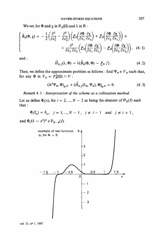
Remark 4 . 1 ; Interprétation of the scheme as a collocation method.

Let us define <£,(*)> for / = 2,..., N - 2 as being the element of PN(7) suchthat :

* , ( y - 8V> y = 1,..., iV - 1 , j # f - 1 and ; * i + l ,

andd\/(l - x 2 ) 2 e P N _ 4 ( / ) .

example of test function <(>,4>, for N = 9

- 1 5 - 1 V - 0 5

-3

-2

1

05 1 y 15

1

2

- 3

vol 21, n° 1, 1987


We defïne then O^ over Q by

®t/2Ù = * < ( * i ) * / * 2 ) f o r a n Y Uj> l ^ U J ^ N - 2 .

This set of éléments of Pjv(fi) is a basis of VN and using this basis as testfunction in (4.3) leads to the following equivalent problem :

j f ï n d ^ e F ^ s u c h t h a t :

where for any function % in C°(Q) we have posed

The scheme (4.3') would be a collocation scheme for the équation (3.28) if thevalues ©yféju) were equal to zero for (fc, /) # (/, j). Since it is not the case, it is acollocation-like method involving nine points at the same time.

Some indications f or the numerical treatment ofthe scheme.

First we want to point out that the expression ofthe nonlinear term we haveused is not only a theoretic tool but has been prefered by Basdevant [1] for theapproximation of the evolutionnary Navier-Stokes équations with periodicboundary conditions. In this latter case the formulation provides an economyof C.P.U. time and input-output.

For the numerical resolution ofthe problem we suggest and itérative methodtreating explicitly the non linear terms : X¥N is the limit of a séquence (v|/£)„ 6 N .

The following method :

^(A2 VN+ ') (£y) = nHNj{K W] fty) 2 < i,j < N - 2,

would involve the inversion of a full and ill conditionned System. Hence, asit is preconised in the littérature we prefer the use of a finite différence precon-ditionning AjD ofthe operator A2 (see Orszag [1], for example)

2 ^ û ' < N - 2 , (4.3")

where e is a relaxation parameter.The évaluation of the explicit right hand side of (4.3") involves two types

of calculus : first the values of a product of two fonctions on the set of (JV + l)2

points %ip secondly the values of the derivative of a function on this set Thefirst calculus is very easy to perform in O(N 2) opérations. The second one is veryexpensive (0(JV4) opérations) directly, in the " physical space ". It can be donein O(N2) opérations, using récurrence formulae in the space of components of



the functions in the bases of Chebyshev polynomials (the spectral space). Thepassage from one space the other one is performed via the F.F.T. algorithm inO(N2 log N) opérations (see Gottlieb-Orszag [1] for more details about thisprocedure). •

Let us introducé a discrete bilinear form aN, defined over VN by :2 ) 6 F i ; (4.4)

and an operator L : PN(Q) -> fV(fi) defined by :

f (LO) Xœ dx = (O, x)M}N , V(O,JQ

Let us set :

J J . (4.5)

Then, an equivalent formulation of problem (4.3) is :

Find x¥NeVN9 such that, for any O e VN :. ^ (4.6)

ûtfOF* O > + < HNJ(\0, Tw)), O > = 0 .

(see (3.22) for the notation 7).We first prove that aN is continuous and elliptic.

LEMMA 4 . 1 : There exist twopositive constants a and 0 independent of N suchthat, for any (O, %)eV2

N \

) ! < a H O l l ^ l l x l l ^ , (4.7)

^ ( 0 , 0 ) ) ^ pil O | | ^ . (4.8)

Proof : We first prove (4.7). Let (O, %) e F£, we have, as in ( 3 . 8 ) :

M ^ X) = ^2O,JV + 2 ^ l l p W + ^ 0 2 ) i V ,

with :

A hUsing (2.8) we obtain :

vol. 21,n° 1, 1987


so that, by intégration by parts :

Thus, it follows from (3.4) that :

I 20 l v l ^ Q E ® ! T (Xl'« = 0 LVJ/V^l/

1/2

x l l l 14 1 (*!,

< Q Ë ©i II *(•, y

Hence, by (2.10) we find :

! Â I < P H <ï) H 11 v 11I ^ 2 0 , i V I ^ ^ II ^ 112,©. Il X II2.JO '

Similarly we get :

U O 2 . N I < c\\ o i |2 i j a | | x ii2(çù-

Finally, from (2.8) we have :

- ^ 1 1 M

4<D

(4.9)

•n

(4.10)

(4.11)

(4.12)

Therefore, (4.7) is a conséquence of (4.10) - (4.12), (3.11), (3.12).Let us prove now (4.8). We keep the above notations but with % = $.

Due to (3.5) and (4.9) we have :

so that, by (2.10), we dérive :

dx\ (4.13)



Similarly, we have :

dxl

Moreover (4.12) and (3.15) give :

0,e>

0

111

(4.14)

(4.15)

Thus, (4.8) is a conséquence of (3.17), (4.13)-(4.15) and the property (2.1). •As in the continuous case (see (3.23)) we can introducé an operator TN :

Jfra-2(Q) - VN by :

aN(TN g, d>) = < g, O > VO e F„ ,

Problem (4.6) is equivalent to the following one :

f Find ^ e Fjv such that :

(4.16)

We consider now a slightly more genera! problem :

ƒ Find (X, Yjy) e IR x FN such that :

1 F ^ VN) ^VN + TN HNJ(k, VN) = 0 . (4.17)

IV. 2. Existence of a solution of the approximate problem and error bound

We shall use now the gênerai theorem concerning the approximation ofproblems stated as (3.32) by problems stated as (4.17) developped in Des-cloux-Rappaz [1]. We have recalled a suitable version of it in the appendix.

First we shall assume in the sequel that the solution T o of (3.28) satisfiesthe following property :

(Xo, o) is a regular point of (3.32).

Let us now prove that lim TN = T. We introducé the projection operators

n^ and n v from V onto VN by :

(1(11 O, x) = Û(O, x), (4.18)

aN(UN O, x) = a(O, %), ^ (4.19)

vol. 21, n° 1, 1987


Using lemma 3.2 and well-known technics upon projection operators we get :

1 O - UN $ ||2 < C inf || O - 0N \\2 .

From (2.7), with r = 2 we dérive that, for any $ in H£(Q) n F (cr ^ 2) :

o

Let us remark now that TN = 11^ o T. The property :

lim TN = T,

o

will be a conséquence of an estimate concerning HN analogous to (4.20).

LEMMA 4 . 2 : There exists a positive constant C, independent of N such that,for any a > 2 and any O e H^(Q) n V ;

o

II (j) _ YI <j) || ^ CN || O || . (4,21)

Proof : Let O be in F n H°(Q\ using (4.8) we have :

|| ( n * - n c J V ) o ii i^ < p - 1 a ^ ^ - n C i N ) ® , ( n w - n a J V ) < D ) .

Next we deduce from (4.18) and (4.19) that :

iN - no j v) o |||A < p - ^ i a((uN - naN) *,(nN - noJV) <P) | +

+ | (a - oN) (UuN 0>, (n^ - UGN) *) I] . (4.22)

Besides, as in the proof of (4.20), we get :

(4.23)

On the other hand, we define for 1 < /, j < 2 :

d4

(4.24)

a 4 /rT- Z

M2 AN Modélisation mathématique et Analyse numériqueMathematical Modelhng and Numencal Analysis

NAVD2R-STOKES EQUATIONS

Then, we have :

(a - O (na>w <t, (ÛN - no>w) <D) = Jt, + 2 J, 2 + J22 .

Setting % = (flN - UaN) O and using (2.8) (see (4.9)) :

113

(4.25)

Using(2.6) and(2.13), noticing that UaN <&(xu .)ePN(I) and that PN reducesto the identity mapping over PN(1) we get :

CN 2 - o

a— 2,a>2

— T-Lui C/ C II 0,<B2

a -2 , . O.ço

Following the same lines as in the proof of (3.12) we obtain :

1 d2 ,A

0,»

so that :

Similarly we obtain :

Finally, noticing that :

nO ; i V

(4.26)

(4.27)

(4.28)

dx\ dx\ C'N N 2N 2

and using (2.8) we check that Jt2 = 0. Hence (4.21) foliows from (2.7), (4.22),(4.23), (4.25)-(4.28). .

vol. 21, n° 1, 1987


According to (4.20) the hypothesis (A. 2) of Theorem A. 1 holds if we choose^v = îlN. In order to prove that hypothesis (A. 1) and (A. 3) holds we computethe derivatives of F and FN. Using (3.26), (3.27) and (3.32) we have, for any(X, <b\ (n,, Xi) eUxV(i=l,2,3):

*) - ƒ)) (4-29)

= 2 :

), (n2= 2 '

r^B(x, Xi)> (I-

x,X2)) + 2T(

i3. X3)) =

l%2, X3) + ^2k)[A., 0] s 0

jJ-i 5(O, x2) + H

^(%3. Xl) + H3 J

Vfc> 4.

2 5(4». Xi))

9(Xi, X2))

(4.30)

(4.31)

(4.32)

Similar formulae are obtained for the derivatives of FN, replacing T by TN

and B by BN and (A. 1) is clearly verified.Moreover it can be checked that (A. 3) is a conséquence of the following

property :

lim || TB{$, x) - TN BN(UN $, n* X) | 2 , a = 0, V(O, %) e V2 .

(4.33)

The following lemma and (4.20) will imply (4.33).

LEMMA 4.3 : There exist two positive constants C and r\ independent of N suchthat, for any (<1>, %) e V2 :

, x) - TN BN(îlN «>, n „ x) Ik» < C [ N - " || O ||2,„ || x ll2>a + (4 ^

+ || $ - n N <D n2<2 il x ll2 « + II x - n w x «2* II * II2,J •

Proo/ : Let (O, x) be in 3>(Q)2. We have :

) ||a + (4

, x) - B(UN O, n N x)) |2dl + I TN(B - 5W) ||

From (3.29) and the regularity of T we have, if 1 < 5 < 3/2 :



so that, by (2.3):

Using (4.21) and the equality TN = TlNo T, we obtain,for any s, 1 < s < 3/2 :

1 (T - TN) 5(O, x) ||2ia < CN'~3'2 || <D \\2jt || x | |2A . (4.36)

Let us consider now the next term in the right hand side of (4.35). We get :

2 , œ - N sein * ( nuo ( 4 3 7 )

Using Theo rem 3.1 and (4.21) we obtain :

11 T II < C (d ^R\

Moreover it foUows from lemma 3.3 that :

11 Rf(f\ v^ R/'TT ff) TT v^ <C /?fCf) v TT v^ -4-

< 7(11 * II2j» II x - n N x II2,0 + II * - n N o ||2iia 11 n N x I I 2 , J •

Hence combining (4.37), (4.38) and the use of (4.20) with a = 2, we get :

TN[B(o>, x) - B(UN *, n* < (c il * II2<a il x - n K x h,» ++ II X Ü2.C0 H O - I l ^ O | | 2 , a ) . (4 .39)

For studying the last term in (4.35) we first notice that, by (4.8) we have,

aN(TN g, S)

Hence, from (4.16) and (4.5) we have :

vol. 21, n° 1, 1987

116 Y. MADAY, B. MÉTF/ET

Moreover, according to the définition of B and BN9 the right hand side of (4.40)can be written as the sum of six expressions.

A typical one is the following :

In order to estimate I, we note that, by (2.8) and an intégration by parts inthe x1 direction :

(4.41)

Since S e VN, then H = (1 - x2)2 A with À(.s y) eIt follows from (3.14) that :

1(4.42)

hence we obtain :

ra,

Applying the estimate (2.13) and (4.26) (with ÔN = S) we obtain :

s) | < c H s

+ (/ - no,,,,) (J - (^ 0 )^ (0 , x)) |o J • (4-43)


NAVŒR-STOKES EQUATIONS

Using (2.4), (2.12) and (2.5) we dérive that, for any 8 > 0 :

117

Il2+e,œ.

v II TT vX II 1XJV X

Similarly, using (2.6) we get :

TT

CN - l + 3 e

x lin^xlk*. (4.45)

Therefore, combining (4.43>(4.45) and setting r\ = inf(3/2 — s, 1 - 3 e)

0 < s < x we obtain :

| 7(0), & H) | A * jft

Similar estimâtes for the other expressions in (4.40) leads to :

n N nN o(4.46)

The desired estimate (4.34) then follows from (4.35), (4.36), (4.39) and (4.46).

•The hypothesis (A. 4) of Theorem A. 1 is checked through :

LEMMA 4.4 : Thereexist monotonically increasing functions

Ck : U+ -• U+, k e M , such thaï, for any (X, S>) G R X VN :

+ H ® «2 J • (4-47)

: By using the expressions of the derivatives of FN (see (4.29)-(4.32))and the upper bound (see (3.33)) :

we shall get (4.47) by the proof of the existence of a constant C > 0, such that,for any (O, %)eV2

N :

vol. 21, n° 1, 1987


First we have

|[ TN BN(®, x) ||2>„ < || TB{d>, x) ||2,„ + || T1?(<D, x) - TN BN(®, X) ||2,a.

(4.49)

Since 11^ <I> = O and llN x = X we have, by (4.34) :

|| TB(®, x) - TN BN(O, x) | 2 , a ^ CN-" || O \\2M || X h,« • (4.50)

Due to (3.29) and Theorem 3.1 we find :

II TB{<S>, x) ||2,a *C\\<b ||2JB || x II 2<a. (4-51)

so that (4.48) is a conséquence of(4.49)-(4.51).Finally let us check the hypothesis (A. 5) of Theorem A. 1. We compute for

(X, <D) 6 R x VN,

* ) •

Using the expression of derivatives of F and FN (see (4.29)), we obtain :

= 2 [T(?i0 £(*„, <t)) - TN(X0 £N(nN ^ 0 , n N O))] +

- ƒ)) - TN(UBN(TlN *0 J n,v T o ) - P* ƒ))] . (4.52)

Note that :

II 7 / - TN Py ƒ ||2>m < II (T - Tw) ƒ ||2(, + 1 T N ( / - ^ ƒ) ||2ia. (4.53)

Since ƒ G #£(Q), p > 1 we deduce from (3.24) and (3.25) that TfeH3(Q.)which is included in H^2(Q) ; from the equality TN = flN o T we get :

lim ||Cr — r K ) / | | 2 > . = 0 . (4.54)JV-^ + OO ~"

Using the continuity of T1N from V into VN, of T from L^(Q) into V we dérive,using (2.12) :

II TN(f - ^v ƒ) ||2,H ^ C || ƒ - £v/ ||0)H < CN-> || ƒ ||PA, (4.55)

hence :

lim || Tf- TNPJ,f\\2^ = 0. (4,56)

Finally (A. 5) is derived from (4.52)-(4.56), (4.20) and (4,34). •


NAVŒR-STOKES EQUATIONS 119

Now we have proved that FN is an approximation of F verifying the hypo-thesis of Descloux-Rappaz [1], we can state the main resuit of this paper,conséquence of Theorem A.L

THEOREM 4.1 :

i) There exist two positive constants Y and 8' < S and, for N ^ No largeenough, a unique C00 mapping *¥N : [XQ — S', Xo + S'] -> VN such that,FN(K YW(X)) = 0and\\ *¥N(X) - UN Wo ||2iffi ^ y foranyXe[X0 - 5\X0 + 8'].

ii) Moreover, if there exist a positive constant Manda real cr > 2 such that :

VX e [Xo - 8', Xo + 6'], 1 ƒ IL - 2 ^ + || ¥(X) \\9A < M , (4.57)

then, there exists a positive constant C, independent of N9 such that :

sup II *P(X) - VN(\) | 2 , . C N 2 " V (4.58)

: The point i) is a direct conséquence of Theorem A. 1. With regard toii), we dérive from Theorem A. 1 that there exists a positive constant C, suchthat, for any X e [Xo - 5', Xo + 5'] :

¥„(*.) ||2-ft ^ C(

From (4.20), we get immediately :

CJV2-" || (X) ||a>„ . (4.59)112.»

Besides, from the définitions of (X), F and FN we obtain :

Ï7 (1 TT XUf\ \\ II «f II 17 /"l TT *Uf\ W J?f\ W/ l Vi II <f

?i | I (T - Tjy) LB0F(X,), *(X)) - ƒ] ||2,a +

2JB + (4.60)

The first term on the right hand side of (4.60) is bounded thanks to (4.59).The second one is studied easily if we note that :

T[BmXl*¥(X))- ƒ]= - ~ T O .

The third one uses the continuity of B (see (4.39)). The last one has been studied

vol 21, n° 1, 1987


in (4.55). Finally denoting 11^ *P(X,) by *¥(%) we can prove that :

|| TN(B - BN)

For this, we are led, as in (4.40), to study expressions as /(^(À,), (k), E) definedat (4.41) for H G VN. Due to (4.43) we have :

S) +0,(Ù

+

each term, on the right hand side of (4.62) are studied similarly by introducing

ox2

0,ü>

(4.63)3 1X,^ x d

If we choose n < - such that 2 < i < a we get from (2.12) and (2.4):

CNl-"[

Using now the following inequality :

and the inverse inequality we dérive after some calculation :

0,Û)


NAVEER-STOKES EQUATIONS 121

The last term in the right hand side of (4.63) is bounded by the same quantityso that (4.58) is proved since || ^(X) ||CT(a can be bounded independently ofX due to the compactness of A.

APPENDIX

THEOREM A. 1 : Let V be a Banach space over M and F : R x V -> V.We assume that :

• F : U x V -> V is a Cp mapping with p ^ 2,• (\0, ô) e R x V vérifies F(X0, ¥<,) = 0 and(X0, ¥<>) is a regular point Le.

D o F(X0, ^ 0 ) is an homeomorphism from V onto V.

Then there exist positive numbers Xo, a and a map :

satisfying the condition :

= 0 and || V(X) - ^Fo ||K ^ a , \/X e ]X0 - Xo, Xö + Xo[.

Furthermore *¥ is of class Cp.In order to approximate the branch { (X), X e ]X0 — Xo, Xo + ^0[ } we

introducé a family of finite dimensional subspaces of F, denoted by VN, N e Nand a family of mappings FN :U x VN -> VN which shall approximate F.

We assume that :

FN : R x VN -• VN are Cp mappings . (A. 1)

We are interestedin solving theequation FN(X, ^^ = 0 in a neighbourhoodof the branch { ¥(X), X e ]X0 - Xo, Xo +X0[ }.

We suppose that the following hypotheses are satisfied :

(i) For any N, there exists a projection operator £PN : V -> VN :

lim | | * - ^ * | | F = 0, V O e F , (A.2)

(ii) for any 0 < k < p - 1 and any fixed (X, O), (Xl9 O J , ..., (Xk, ®k) inIR x F , we have :

lim || F<*KK ®) (K « i , ^ 2 5 *2, - ^ **)iV^^ oo

- FP(\, 0>„ O) (Xlf v O l 5 . . . . Xk) ^ <D,) IK = 0 (A. 3)

vol. 21, n° 1, 1987


(iii) there exist positive constants r\, Cu ..., Cp such that VN 6 N,

VA: e { 1, ...,p } , V(A, Q>)eUxVN with (| X - Xo | + || O - &N

(iv)

lim Sup || F ' 1 ' ^ , <D0) (X, <D) - F ' 1 ^ , ^ * 0 ) (X, <D) ||K = 0 .N-* QO a,4>) e R x VN

Hl + | | O | | r = l

(A. 5)

T / ^ there exist No e AT*, positive constants À,o, a', p and for N ^ JV0, a wmçwé?

mapping ^x : \e]X0 — X'Oi Xo + X'o[ ^> ¥N(X) e VN satisfying the conditions :

VX e ]X0 - l'ot Xo + X'o[ 9 FN(X, VN(X)) - 0 and || *¥N(X) - 0>» Wo \\v ^ a'

*¥N isof class Cp with bounded derivatives uniformly with respect to X andN.

Furthermore, X'o < ^ 0 and we have :

îvW ||K < P(H F*&* »n ¥») Wv + II • M ~ &„ M-) Wv),\/Xe]X0 -X'0,X0 +X'0[ m

REFERENCES

R. A., ADAMS, [1] Sobolev spaces ; Academie Press (New York, San Francisco, London)1975.

C. BASDEVANT, [1] Le modèle de simulation numérique de turbulence bidimensionnelledu LM.D. ; Note interne du L.M.D. n° 114 (juin 1982).

J. BERGH, J. LOFSTROM, [1] Interpolation spaces — an introduction; Springer-Verlag(Berlin, Heidelberg, New York) 1976.

C. BERNARDI, C CANUTO, Y. MADAY> [1] Generalized inf-sup. condition for Chebyshev

approximation of the Navier-Stokes équations ; ICASE report 1986-63.C. BERNARDI, Y. MADAY, B. MÉTIVET, [1] Spectral approximation ofperiodicjnonperiodic

Navier-Stokes équations ; to appear, in Numer. Math.[2] Calcul de la pression dans la résolution spectrale du problème de Stokes. Aparaître dans la « Recherche aérospatiale », 1986.

C. BERNARDI, G. RAUGEL, [1] Méthodes d'éléments finis mixtes pour les équations deStokes et de Navier-Stokes dans un polygone convexe ; Calcolo 18-3 (1981).

C. CANUTO, Y. MADAY, A. QUARTERONI, [1] Combined finite element and spectral

approximation of the Navier-Stokes équations ; Numer. Math. 44, 201-217 (1984).C. CANUTO, A. QUARTERONI, [1] Approximation Resultsfor Orthogonal Polynomials in

Sobolev Spaces, Math, of Comp. 38, (1981), 67-86.J. DESCLOUX, J. RAPPAZ, [1] On numerical approximation of solution branches of non

linear équations; R.A.I.R.O. Numer. Anal. 16-4, 319-350 (1982).M. DEVILLE, L. KLEISER, F. MONTIGNY, [1] Pressure and time treatment of a Stokes

problem, Int. Journal for Num. Methods in Fluids, 1984.M2 AN Modélisation mathématique et Analyse numérique

Mathematical Modelling and Numerical Analysis


V. GIRAULT, P. A. RAVIART, [1] Finite Element Approximation of the Navier-Siokeséquations, Theorie and Aigorithms ; Springer-Verlag (1986).New York (1979).

D. GOTTLIEB, S. À. ORSZAG, [1] Numericol anaîysis of spectral methods : Theory andapplications ; CBMS — NS F Régional Conference Series in Applied Mathema-tics, SIAM, Philadelphie 1977.

P. GRISVARD, [1] Espaces intermédiaires entre espaces de Sobolev avec Poids; Ann.Scuola Norm. Sup. Pisa, 17, 1963.

L. KLEISER, U. SCHUMANN, [1] Treatment of Incompressibility and Boundary Conditionsin 3-D Numerical Spectral Simulations of Plane Channel Flows, proceedings ofthe Third GAMM Conference on Numerical Methods in Huid Mechanics,Viewig-Verlag, Braunschweig (1980), 165-173.

P. LE QUERE» T. ALZIARY de ROQUEFORT, [1] Sur une méthode spectrale semi implicitepour la résolution des équations de Navier-Stokes d'un écoulement bidimensionnelvisqueux incompressible ; C.R. Acad. Se. Paris, 294 (3 mai 1982), Série II, p. 941-944.

L L. LIONS, [1] Quelques méthodes de résolution de problèmes aux limites non linéaires,Dunod, 1969.

Y. MADAY, [1] Anaîysis of spectral operators in one dimensional domain ; ICASE report1985, 17.[2] Some spectral methods concerning a 4th order l-D problem ; to appear.[3] Pseudo-spectral operators in multi-dimensional domains-application to Navier-Stokes problem ; to appear.

Y, MADAY, B. MÉTIVET, [1] Estimations d'erreur pour l'approximation des équations deStokes par une méthode spectrale ; la « Recherche aérospatiale », 4, (1983), p. 237à 244.

Y. MADAY, A. QUARTERONI, [1] Spectral and pseudo-spectral approximations of Navier-Stokes équations ; S.I.A.M. J. Numer. Anal 19 (1982).[2] Legendre and Chebyshev spectral approximation of Burger's équations ; Numer.Math., 37 (1981).[3] Approximation o f Burger's équations by pseudo-spectral methods ; R.A.I.R.O.An. Num. 16-4(1982).

M. R. MALIK, T. A. ZANG, M. Y. HUSSAINI, [1] A spectral collocation methodfor theNavier-Stokes équations, « ICASE Report » n° 84-19.

B. MÉTIVET, [1] Résolution des équations de Navier-Stokes par méthodes spectrales.Thèse, Université P. & M. Curie (1987).

B, MÉTIVET, Y. MORCHOISNE, [1] Multy domain spectral technique for viscousflow calcu-lations. « ONERA » T. P, n° 1981-134.

Y. MORCHOISNE, [1] Résolution des équations de Navier-Stokes par méthode pseudo-spectrale en espace-temps ; la « Recherche Aérospatiale » 5, (1979), pp. 293-306.

R. D. MOSER, P. MOIN, A. LÉONARD, [1] A spectral numerical methodfor the Navier-Stokes équations with application to Taylor Couette flow ; JCP — 52(1983), pp. 524-544.

S. A. ORSZAG, [1] Spectral methods forproblems in complex geometries ; J.C.P. 37 (1980),pp. 70-92.

S. A. ORSZAG, M. ISRAELI, M. DEVILLE, [1] Boundary Conditions for IncompressibleFlows ; to appear.

S. A. ORSZAG, A. T. PATERA» [1] Secondary instability of wall-bounded shear flows ;J. Fluid Mech., 128 (1983).

R. VOIGT, D, GOTTLŒB, M. Y. HUSSAINI, [1] Proc. of Symposium on Spectral methodsfor Partial Differential Equations, SIAM Philadelphia (1984).

vol. 21, n° 1, 1987

Documents

Chebyshev spectral approximation of Navier …...HMW IMOâJSATMW MATHÉMATIQUE ET ANALYSE HUNÉftKKIE (Vol 21, n 1, 1987, p 93 à 123) CHEBYSHEV SPECTRAL APPROXIMATION OF NAVIER-STOKES