Solving the SVM Problem

Christopher Sentelle, Ph.D. CandidateL-3 CyTerra Corporation

Introduction

SVM Background

Kernel Methods

Generalization and Structural Risk Minimization

Solving the SVM QP Problem

Active Set Method Research

Future Work

Introduced by Vapnik (1995)

Binary classifier

Foundation in statistical learning theory (Vapnik)

Excellent generalization performance

Easy to use

Avoids curse of dimensionality

Avoids over-training

Single global optima

Burges, C., “A Tutorial on Support Vector Machines for Pattern Recognition”

Support Vector Machine seeks maximal margin separating hyperplane

The maximum margin provides good generalization performance

Support vectors lie on the margin and define the margin

2

2

1min

2

s.t. , 1 0i i

w

y w x b

1

wMargin

Non-optimal hyperplane with small margin

Optimal hyperplane has largest margin

Support Vector

-3 -2 -1 0 1 2 3 4-2.5

-2

-1.5

-1

-0.5

0

0.5

1

1.5

2

2.5

In many cases, problem is not linearly separable

Soft-margin formulation introduces slack variables to allow some data points to cross margin

C is a tunable parameter

2

2

1min

2

s.t. , 1i i

i

i

i

w

y w x b

C

Penalty term

Slack variable

The SVM problem formulation can be recast to dual through method of Lagrange multipliers

1 1 1

1

1

1 , 1

1, , 1

2

0

0

1,

2

, ,N N N

i i i i i i i

i i i

N

i i i

i

N

i i

P

i

i i

i

N N

D i i j i j i j

i i j

L y x b u

Ly

w

Ly

b

L

b C

L

C u

y y xx

w w wα

w

w

x

Dual-formulation SVM Quadratic Programming Problem

Bound SVs, cross margin with non-zero slack ( )

Non-bound SVs, on margin

Non SVs ( )

,

1,

2

. .

m

0 , 0

ax i i j i j i j

i i j

i i i

i

y y x

s t C

x

y

Data points appear within dot product

Convex, Quadratic objective

Single equality constraintPenalty parameter, C, shows up in bound

constraints

1, 0i iy 1, 0i iy

1,0i i Cy 1,0i iy C

i C

C

0C0

Kernel methods can be applied to SVM dual formulation

Kernel represents dot-product formed in a non-linearly mapped space

Unnecessary to know or form mapping

,

m1

2

. . 0 , 0

ax ,i i j i j

i i j

i i

i j

i

i

y y k x

s t C y

x

, ,i j j jk x x x x

.

A chosen kernel function must satisfy Mercer’s Condition (Vapnik, 1995)

Common kernel functions:

2

A kernel function , satisfies Mercer's condition

if for all functions, , such that is finit

0

e

,

g x

K x y

g x

K x y g x g y dxd

dx

y

Polynomial

Gaussian RBF

Sigmoid

Linear

, 1d

k x y xy

2

22, e

x y

k x y

, ,k x y x y

, tanh ,k x y x y

**RBF kernel most commonly employed since it is numerically stable and can approximate a linear kernel.

A slightly different problem is solved for Support Vector Regression (SVR):

ν -SVC trades the parameter, C, in classification for a parameter, ν, that pre-specifies proportion of support vectors

2 2 2minimize

1 ˆ2 2

subject to ,

ˆ,

i i

i

i i i

i i i

Cw

w b

y

x y

w x b

21 1

2

subject to

minimi

0, 0

ze

,

i

i

i i i

i

wl

y x w b

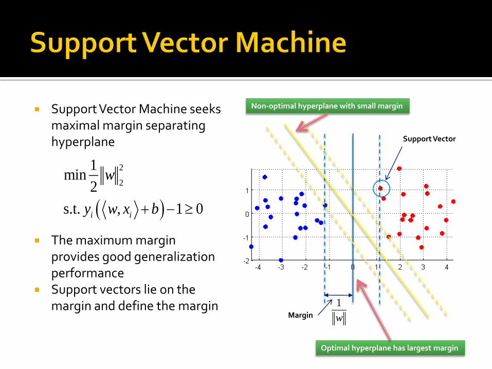
Typically a neural network minimizes the empirical risk

(Vapnik, 1995) introduces the following risk bound:

For some with probability less than

Where is the VC (Vapnik-Chervonenkis) dimension , a measure of capacity

Vapnik introduced notion of “Structural Risk Minimization” “Perform trade between empirical error and hypothesis space complexity”

1

1,

2

l

emp i i

i

fl

R y x

log 2 1 log 4

emp

hR

l

l hR

h

0 1 1

Capacity or VC-dimension is related to how many points can be arbitrarily labeled and correctly fit by a set of functions,

In this example, 3 data points are “shattered” by the line function (VC dimension is 3)

f

Example from Burges, C., “A Tutorial on Support Vector Machines for Pattern Recognition”

LIBSVM (SMO) Commercially available: http://www.csie.ntu.edu.tw/~cjlin/libsvm/

SVMLight (Decomposition w/ Interior Point) http://www.cs.cornell.edu/People/tj/svm_light/

SVMTorch (Decomposition for Large-Scale Regression) http://bengio.abracadoudou.com/SVMTorch.html

SVM-QP (Active Set method) https://projects.coin-or.org/OptiML

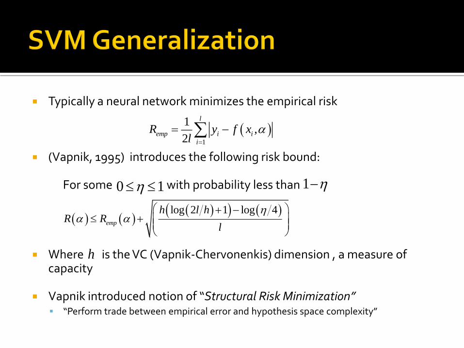
SVM dual formulation

Convex, quadratic, bound-constrained, single equality constraint

Problem is large

Q (kernel matrix) is dense, semi-definite, ill-conditioned

Equality constraint is considered “nuisance” for some algorithms

Ci

0 ,0 s.t.

min

αy

α1Qαα

T

TT

α

nn

jijiji xxKyy ,,Q

0αyT

Karush-Kuhn Tucker (KKT) conditions for optimality are necessary and sufficient, given convexity, for optimality

1, , , ) 1 ( ) ( 1 )

2

1 0

0

0

0

0

0

( )

(

0

T T T T TD

T

i

i

i

i i

i i

r Q y r C

Q

r

C

L

y r

y

C

r

Complementary conditions

Feasible region

Non-negativity constraints on KKT multipliersfor inequality constraints

Chunking

Decomposition

Active SetGeometricalConvex Hull

Interior Point(SVMLight)

Gradient Projection

Primal Methods

Cutting Plane(SVMPerf)

Interior Point

SMO

Gradient Projection

Stochastic Sub-gradient

PegasosSVM-QP

SVM-RSQP

SimpleSVM

DirectSVMVariable

Projection

Single Equality Constrained GP

Regularization Path Search

Max Violating Pair WSS

Quadratic info WSS

Maximum Gain WSS

Incremental/Decremental

Training

Low-Rank Kernel Approx

OOQP for Massive SVMs

*This represents only a sampling ofoptimization methods reported in the literature

VapnikIntroduces SVM

Decomposition method breaks problem down into sequence of fixed-size sub-problems

Variables are optimized while the set of variables remain fixed

Objective decreased at each iteration as long as KKT violators added to sub-problem and non-KKT violators switched out Proof of linear convergence (Keerthi, Lin, et al.)

min 2 1

. . y ,

1

2

0

w

T T Tww ww w wn n w w

T Tw w n n w

Q Q

s t y C

w n

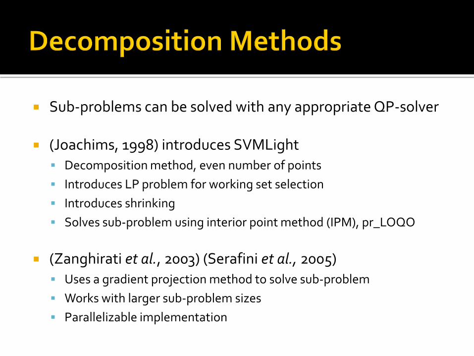
Sub-problems can be solved with any appropriate QP-solver

(Joachims, 1998) introduces SVMLight Decomposition method, even number of points

Introduces LP problem for working set selection

Introduces shrinking

Solves sub-problem using interior point method (IPM), pr_LOQO

(Zanghirati et al., 2003) (Serafini et al., 2005) Uses a gradient projection method to solve sub-problem

Works with larger sub-problem sizes

Parallelizable implementation

SMO (Sequential Minimal Optimization, Platt 1999) takes decomposition to extreme by optimizing 2 data points at a time

Sub-problem has analytical solution

Optimal solution clipped to maintain feasibility

1 2

11 22 1

2 2 2 1 1

1

2 2

2

, y

2 ,

T T

i

j

i

N

j j j i

E Ey y

K K K yE bK y

1 0

2 0

2 0

2 C

2 C

1 0

1 C

1 C

1 2y y

1 2y y

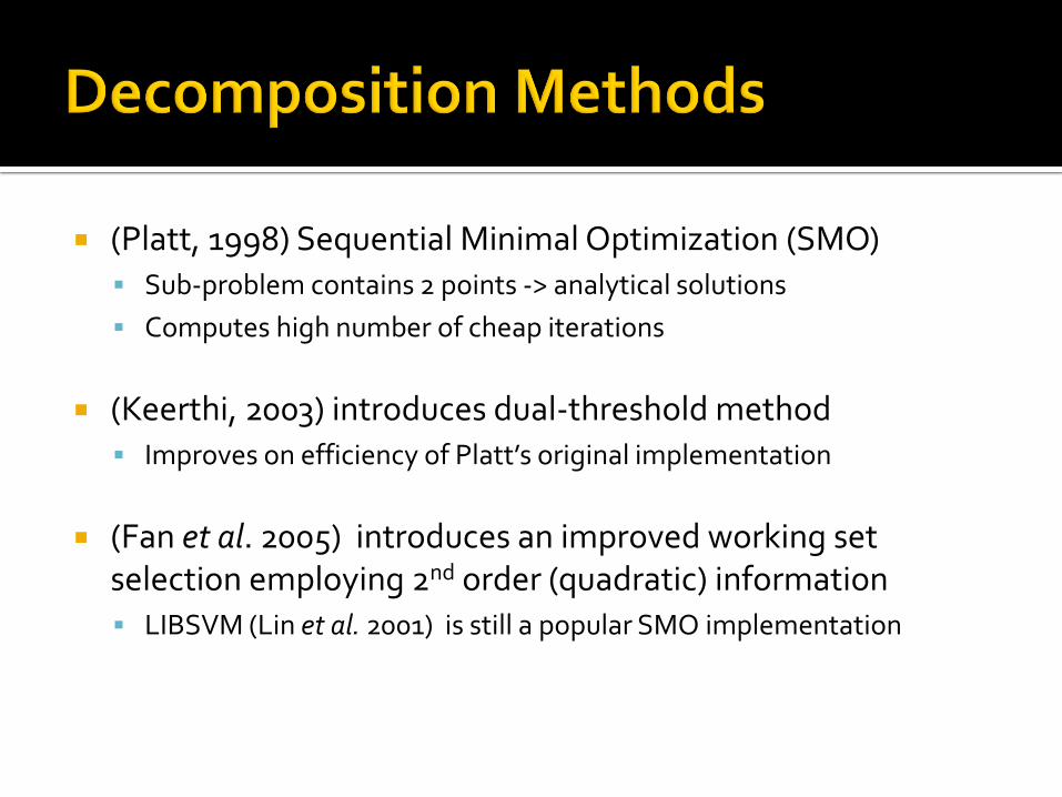
(Platt, 1998) Sequential Minimal Optimization (SMO) Sub-problem contains 2 points -> analytical solutions

Computes high number of cheap iterations

(Keerthi, 2003) introduces dual-threshold method Improves on efficiency of Platt’s original implementation

(Fan et al. 2005) introduces an improved working set selection employing 2nd order (quadratic) information LIBSVM (Lin et al. 2001) is still a popular SMO implementation

Given an inequality constrained problem

Goal is to identify active constraints in solution, i.e. inequality constraints satisfied as equality constraints

Active set method incrementally identifies active constraints and solves corresponding equality constrained problem until all inequality constraints are satisfied

11

2

. .

mi

n T TQ

s t Ax b

Cx d

Equality constrained problem is solved given current set of active constraints

Violated inactive constraints identified and single inactiveconstraint converted to activeconstraint and problem resolved

[ ]

11

2

. .

min

,

T T

i i

Q

s t Ax b

C ix d

Activeset

The active set method exploresfaces of convex polytope formedfrom set of inequality constraints

Incremental nature allows use of efficient rank-one updates to factorizations used to solve equality-constrained problem

Ideal for medium-sized problems with few support vectors (sparse solution)

Memory still issue for large problems, can employ

Preconditioned Conjugate Gradient

Kernel Approximations

The active set method exploresfaces of convex polytope formedfrom set of inequality constraints

(Cauwenberghs, et al., 2000) Introduce an active set method for incremental/decremental training

Method is only applicable to positive definite kernels

(Vishwanathan et al., 2003) Introduce an active set method (SimpleSVM)

Initializes the method using the closest pair, opposite label, points

Mentions possibilities for, but does not handle the singular Kernel matrix case

(Shilton et al., 2005) Solve a min-max problem or primal-dual hybrid problem

Avoids working with the equality constraint

(Vogt et al., 2005) Does not address the case of a semi-definite or singular Kernel matrix

Suggests a gradient projection be used to speed-up active set method

(Scheinberg et al., 2005) Introduces efficiently implemented dual Active Set method

Handles semi-definite kernels

Shows competitive results against SVMLight

(Sentelle et al., 2009, in work) Introduces Revised Simplex, avoids singularities common to Active Set

methods

Based upon the penalty barrier method Replace inequality constraints with

penalty function

becomes

Optimality conditions become:

0 ln( )i ixx

1

2

. . Ax=b, x 0

min T T

xc x x Qx

s t

1

1

2

. . Ax

min ln

=b

NT T

jx

j

c x x Qx x

s t

1

1

1 2

11 2

1, )

2

( ) ln

( , ) 0

where ( , ,... )

( ,

0

( , ,. . )

0

. ,

T TD

NT

j

j

T

n

n

L x x

c Qx A e

Ax b

c x Qx

Ax b x

V

e

x s

V diag x x x

S diag s s s s

VSe

V e

Newton’s method employed to find solution to optimality conditions

Which for IPM, the Newton step becomes

In IPM, complementary conditions not maintained, met at solution

Ideal for dense Hessians and large problems

Kernel approximation methods proposed to allow method to deal with non-linear kernels

Polynomial convergence, theoretical worst case is O(n)

1

( )

( )

nn n

n

f xxx

f x

0 0

0

T T s Qx

e V

A b Axx

Q A I c

S

A

s eS V

, ,T n kQ L L D L k n

(Fine & Scheinberg, 2001) Implements a primal-dual interior point method (Mehrotra prediction-

corrector)

Problem solved at each iteration grows cubically with problem size

Employ Kernel approximation to reduce computations at each iteration

Employ Incomplete Cholesky factorization

(Ferris & Munson, 2003) Discuss application of IPM to large-scale SVM problems

(Gondzio & Woodsend, 2009) Show how use of separability allows scaling of IPM to large-scale

problems (outperforms all but LIBLinear on large problems)

Try to solve the primal problem instead of dual

Traditionally, dual admits easier use of kernel matrix

Dual solution not always “sparse”

Primal converges to approximate solution quicker (Chapelle, 2006)

21minimize

2

s.t. , 1 0

i

i

i i i

C

y b

w

w x

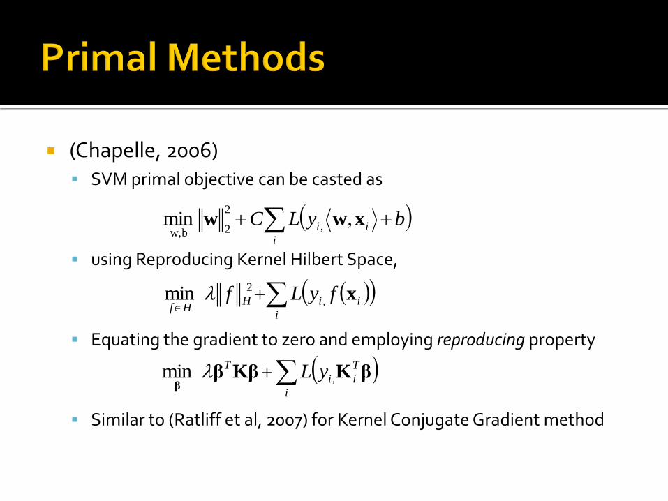
(Chapelle, 2006) SVM primal objective can be casted as

using Reproducing Kernel Hilbert Space,

Equating the gradient to zero and employing reproducing property

Similar to (Ratliff et al, 2007) for Kernel Conjugate Gradient method

i

ii byLC xww , min ,

2

2bw,

i

iiHHf

fyLf x,

2 min

i

T

ii

T yL βKKβββ

, min

(Joachims, 2006) introduces SVM-Perf Cutting planes method

Shows considerable improvement over decomposition methods for linear kernels

Convergence is

(Shalev-Shwartz et al., 2007) introduce Pegasos Employs stochastic gradient descent, sub-gradient, trust-region

Solves text classification problem (Reuters Corpus Volume 1) with 800,000 points < 5 sec!!!!

Linear kernels only

Convergence is

21O

1O

Works by projecting gradient onto convex set of constraints

Activates/deactivates more than one constraint per iteration

(Dai & Fletcher, 2006) introduce single-equality constrained Gradient Projection for SVM

gradient

projected gradient

x0

xdGxxx

gx

x

TT

o

q

tPx(t)

(t))q(

21

t

)(

, where

min

(Wright, 2008 NIPS conference) suggests application of primal-dual gradient projection to SVM problem

Consider saddle point (min-max) problem

where is convex for all and is concave for all

Projection steps are as follows:

xvlXxVv

,maxmin

xl , Xx ,vl Vv

11

1

,

,

kk

vk

k

V

k

kk

xk

k

X

k

xvlvPv

xvlxPx

(Zhu et al., 2008) “An efficient primal-dual hybrid gradient algorithm for total variation image restoration, ” Tech Report, UCLA

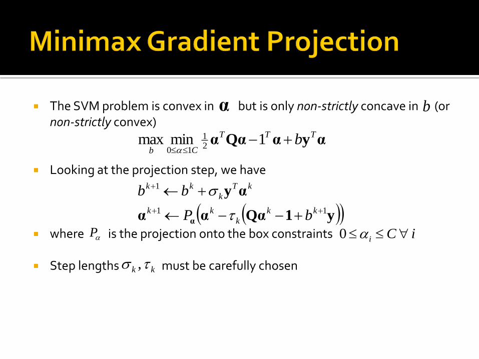
The SVM problem is convex in but is only non-strictly concave in (or non-strictly convex)

Looking at the projection step, we have

where is the projection onto the box constraints

Step lengths must be carefully chosen

αyαQααTTT

Cbb

1 minmax

21

10

α b

y1Qααα

αy

α

11

1

kk

k

kk

kT

k

kk

bP

bb

P iCi 0

kk ,

Can we further improve training algorithms for large datasets?

Popular SMO algorithm is a coordinate descent method

Care must be taken to ensure numerical stability

Data scaling affects convergence speed

Improper setting of C value and/or kernel parameters can prevent convergence

May be slow, overall, when compared to other methods

Other non-decomposition methods introduced in SVM community cannot handle large training set sizes

Our goal is to find non-decomposition techniques that can handle large training sets and are fast

Given the equality-constrained problem solved at each iteration, a direction of descent can be solved (for SVM)

In general, system of equation is indefinite, possibly singular

Several factors cause singularity

Kernel-type (linear kernel)

Subset of chosen non-bound support vectors

Singularities can occur for positive definite kernels!

dg

ch

y

yQT

s

sss

0

Positive semi-definite sub-matrix of original Kernel matrix containing non-bound SVs

(Rusin, 1971) Revised Simplex Introduces revised simplex for quadratic programming

Equality-constrained problem solved at each iteration guaranteed non-singular

Represents a form of inertia controlling method

(Sentelle et al., 2009) Adapt Revised Simplex to SVM Optimize method for SVM problem

Employ Cholesky factorization with rank-one updates (similar to Scheinberg 2006)

Show method can be viewed as a “fix” to existing active set methods which must contend with singularities

Conventional active set methods typically solve equality constrained problem of activeconstraints, directly

Solving for descent direction allows deletion of existing constraint before adding new constraint

Conventional active set method does not maintain complementary conditions during descent

Maintaining complementary conditions are key to guaranteeing non-singular equations

c

T

c

csc*

s

T

s

sss

αy

αQ1α

y

yQ

*0

*0

si

i

q

y

*ss s s s

Ts

Q αy α

y

0

1

0

s

g

ss s s

Ts

sc c ss s s

Q y h

y

Q α Q α y

00

is

T

s

sss eh

y

yQ

g

Indefinite, non-singular matrix admits use of NULL-space method for solution

Given the system

Define NULL space as

System of equations becomes

Solving for

A Cholesky factorization is maintained

Null space has an analytical solution

Efficient rank-one updates made to Cholesky factorization without typical QR factorizations

0, Ts z yZy h Zh Yh

ss z ss y s

Ts y

Zh Q Yh y g u

y Yh v

Q

0

ss s

Ts

Q y h u

g vy

( )T Tss z yZh Z u Q hZ Q Y

zh

T TssQ Z R RZ

1 2 1... ny yy yZ

I

• Adult-a has 32,000 data points• Cover Type has 100,000 data points• 10-2 stopping criterion

Improved speed and memory consumption alternatives still being investigated

Gradient project steps can be inserted to move multiple constraints per iteration

Conjugate gradient can be applied to reduce memory consumption

Problem becomes increasingly ill-conditioned as progress made towards solution

Care must be taken to ensure conditions of non-singularity maintained despite accuracy of conjugate gradient solution

(Vapnik, 2009) has introduced Learning Using Privileged Information (SVM+)

Makes use of additional information available during training to speed up converge

Examples of privileged information Future stock prices

Radiographer notations in tumor classification task

Additional annotations made in handwriting recognition task

Our method can be applied to this formulation

Questions?