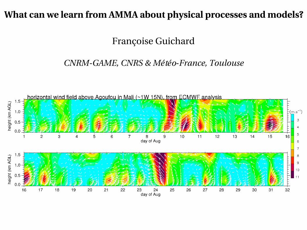
What can we learn from AMMA about physical processes and models?

Françoise Guichard 

CNRM­GAME, CNRS & Météo­France, Toulouse

OUTLINE

1) broad context

2) modelling 

       • large scale [GCMs along a N­S transect, AMMA­CROSS]

       • mesoscale [comparison of mesoscale simulations of an MCS]

(documenting current state, pointing to specific issues)

3) analysis of data [surface climate and radiative budget)]

• seasonal & diurnal cycle in the Sahel, interannual variability

• contrasting Sahelian & Soudanian sites

(including comparison with ECWMF IFS)

4) summary

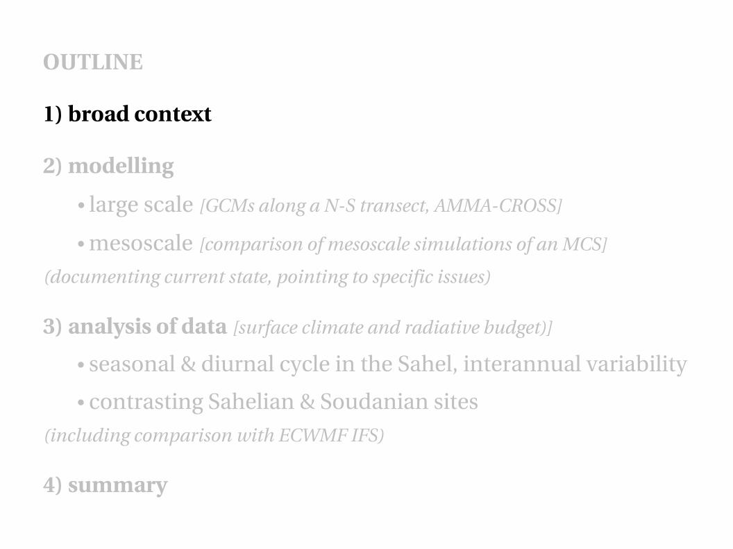
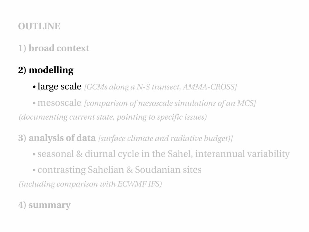
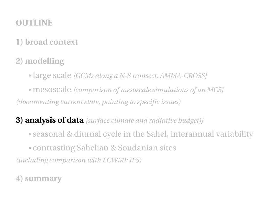
OUTLINE

1) broad context

2) modelling 

       • large scale [GCMs along a N­S transect, AMMA­CROSS]

       • mesoscale [comparison of mesoscale simulations of an MCS]

(documenting current state, pointing to specific issues)

3) analysis of data [surface climate and radiative budget)]

• seasonal & diurnal cycle in the Sahel, interannual variability

• contrasting Sahelian & Soudanian sites

(including comparison with ECWMF IFS)

4) summary

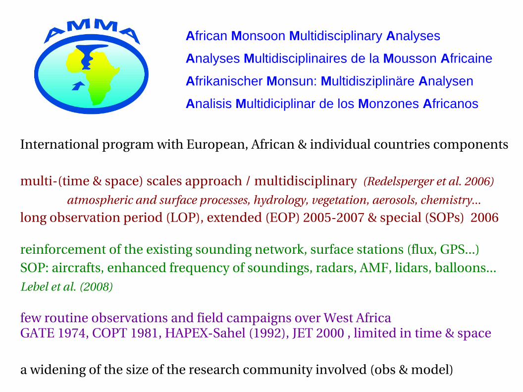
International program with European, African & individual countries components

multi­(time & space) scales approach / multidisciplinary  (Redelsperger et al. 2006) 

atmospheric and surface processes, hydrology, vegetation, aerosols, chemistry...

long observation period (LOP), extended (EOP) 2005­2007 & special (SOPs)  2006

reinforcement of the existing sounding network, surface stations (flux, GPS...) SOP: aircrafts, enhanced frequency of soundings, radars, AMF, lidars, balloons...Lebel et al. (2008)

few routine observations and field campaigns over West Africa GATE 1974, COPT 1981, HAPEX­Sahel (1992), JET 2000 , limited in time & space

a widening of the size of the research community involved (obs & model)     

African Monsoon Multidisciplinary Analyses

Analyses Multidisciplinaires de la Mousson Africaine

Afrikanischer Monsun: Multidisziplinäre Analysen

Analisis Multidiciplinar de los Monzones Africanos

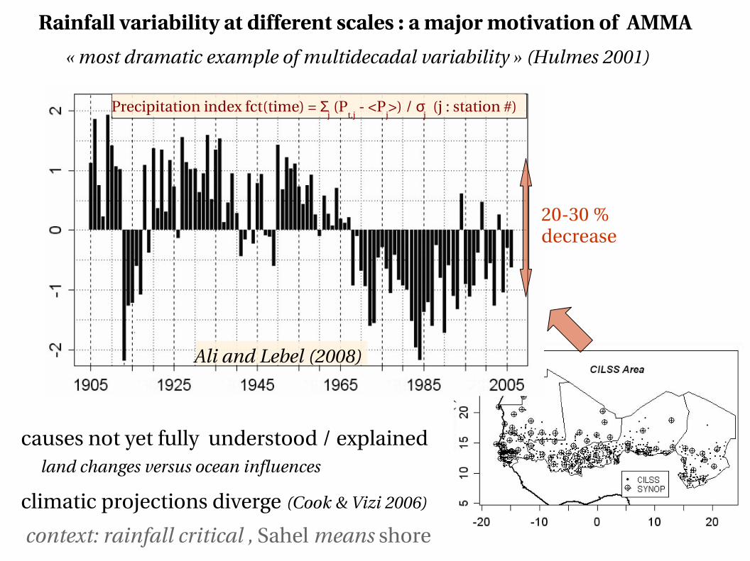
Rainfall variability at different scales : a major motivation of  AMMA 

Precipitation index fct(time) = Σj (P

t,j ­ <P

j>) / σ

j  (j : station #)

Ali and Lebel (2008)

causes not yet fully  understood / explained     land changes versus ocean influences

climatic projections diverge (Cook & Vizi 2006)

« most dramatic example of multidecadal variability » (Hulmes 2001)

20­30 % decrease 

context: rainfall critical , Sahel means shore

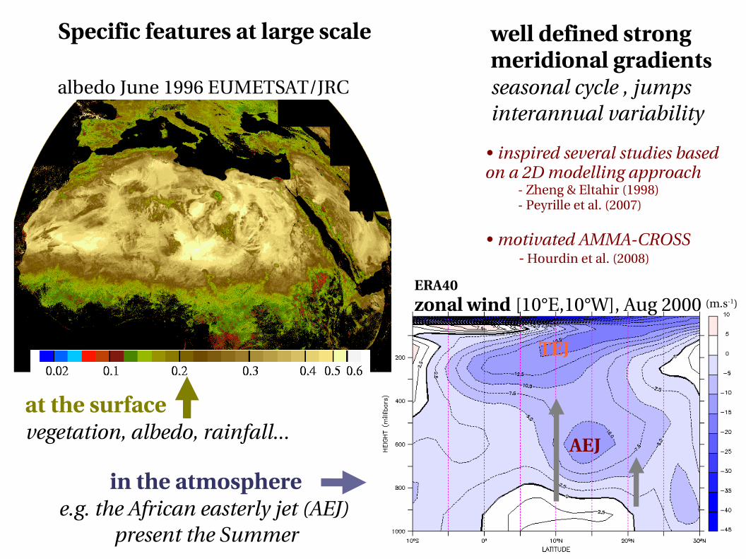
albedo June 1996 EUMETSAT/JRC

at the surfacevegetation, albedo, rainfall...

zonal wind [10°E,10°W], Aug 2000 

well defined strong meridional gradientsseasonal cycle , jumpsinterannual variability

Specific features at large scale

in the atmospheree.g. the African easterly jet (AEJ) 

present the Summer

• inspired several studies based on a 2D modelling approach

­ Zheng & Eltahir (1998)­ Peyrille et al. (2007)

• motivated AMMA­CROSS ­ Hourdin et al. (2008)

AEJ

(m.s­1)

TEJ

ERA40

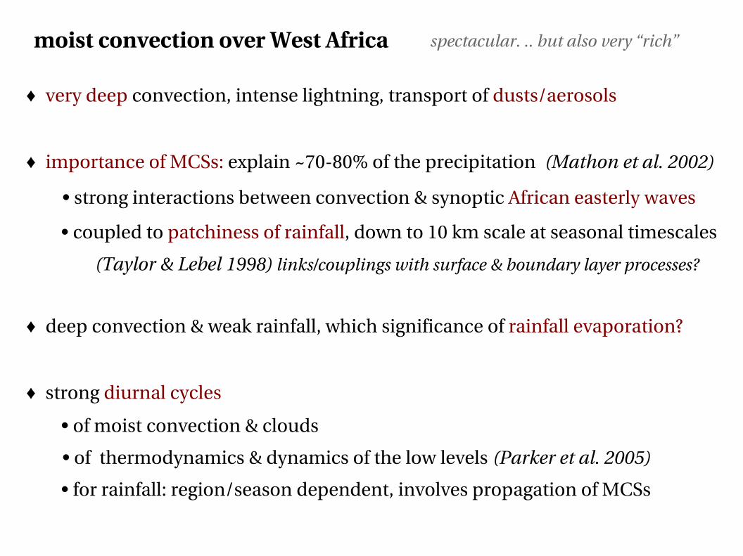
moist convection over West Africa

♦  very deep convection, intense lightning, transport of dusts/aerosols

♦  importance of MCSs: explain ~70­80% of the precipitation  (Mathon et al. 2002)

        • strong interactions between convection & synoptic African easterly waves

• coupled to patchiness of rainfall, down to 10 km scale at seasonal timescales

                (Taylor & Lebel 1998) links/couplings with surface & boundary layer processes?

♦  deep convection & weak rainfall, which significance of rainfall evaporation? 

♦  strong diurnal cycles 

• of moist convection & clouds 

        • of  thermodynamics & dynamics of the low levels (Parker et al. 2005)

  • for rainfall: region/season dependent, involves propagation of MCSs

spectacular. .. but also very “rich”

surface & low atmospheric levels

♦ thought to be key elements of the West African monsoon            starting  from Charney (1975), Gong & Eltahir (1996)

•  ≠   space and time scales (paleo to diurnal, meso scales ) •  ≠  mechanisms of surface­atmosphere interactions

♦ mechanisms not well  known/quantified , not all known

♦   not much studies on low clouds & aerosols

♦ hypotheses, controversies in past decades          academic & GCM­based studies, useful but few data available for guidance / testing

factors controlling surface fluxes & their variations ?limited dataset from SEBEX/HAPEX­Sahel 

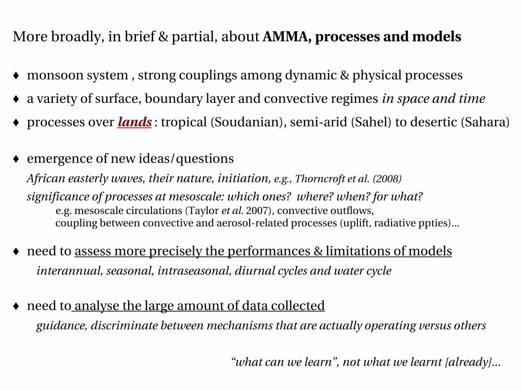
More broadly, in brief & partial, about AMMA, processes and models

♦ monsoon system , strong couplings among dynamic & physical processes

♦ a variety of surface, boundary layer and convective regimes in space and time 

♦ processes over lands : tropical (Soudanian), semi­arid (Sahel) to desertic (Sahara)

♦ emergence of new ideas/questions

     African easterly waves, their nature, initiation, e.g., Thorncroft et al. (2008)

     significance of processes at mesoscale: which ones?  where? when? for what?                e.g. mesoscale circulations (Taylor et al. 2007), convective outflows,                   coupling between convective and aerosol­related processes (uplift, radiative ppties)...  

♦ need to assess more precisely the performances & limitations of models 

interannual, seasonal, intraseasonal, diurnal cycles and water cycle 

♦ need to analyse the large amount of data collected 

guidance, discriminate between mechanisms that are actually operating versus others

                                                                                 “what can we learn”, not what we learnt [already]...

OUTLINE

1) broad context

2) modelling 

       • large scale [GCMs along a N­S transect, AMMA­CROSS]

       • mesoscale [comparison of mesoscale simulations of an MCS]

(documenting current state, pointing to specific issues)

3) analysis of data [surface climate and radiative budget)]

• seasonal & diurnal cycle in the Sahel, interannual variability

• contrasting Sahelian & Soudanian sites

(including comparison with ECWMF IFS)

4) summary

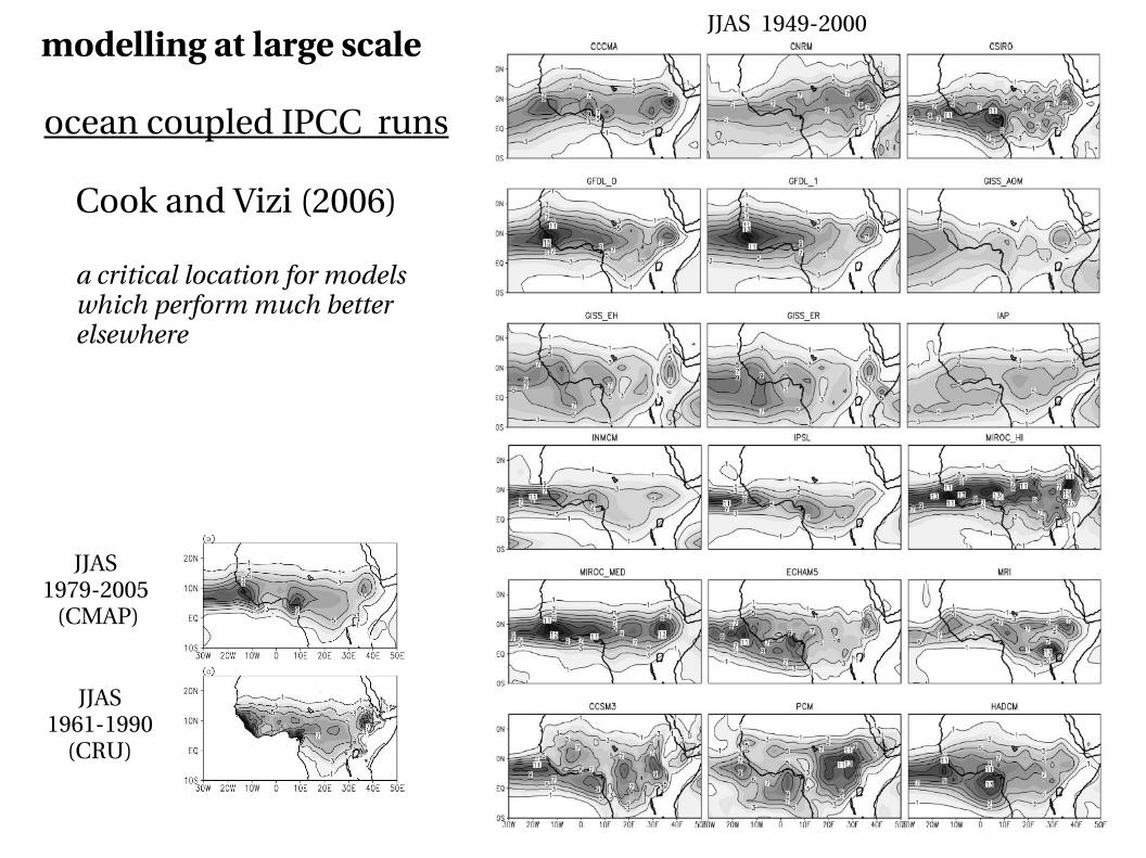
Cook and Vizi (2006)

a critical location for modelswhich perform much better elsewhere

JJAS 1979­2005 

(CMAP)

JJAS 1961­1990 

(CRU)

JJAS  1949­2000 modelling at large scale

ocean coupled IPCC  runs

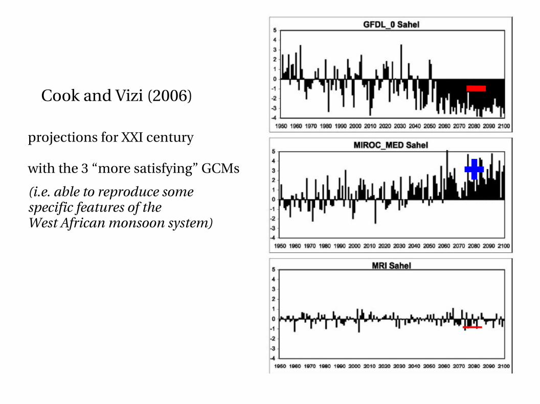
projections for XXI century 

with the 3 “more satisfying” GCMs

(i.e. able to reproduce some specific features of the West African monsoon system) 

Cook and Vizi (2006)

GCMs/RCMs with

prescribed SST

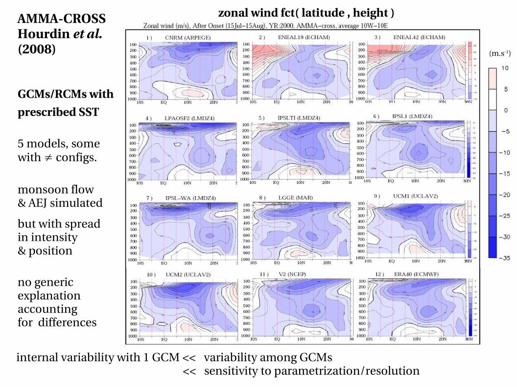
5 models, some with ≠ configs.

monsoon flow & AEJ simulated

but with spread in intensity & position

no generic explanationaccounting for  differences

internal variability with 1 GCM <<   variability among GCMs                                                               <<   sensitivity to parametrization/resolution

AMMA­CROSS Hourdin et al. (2008)

zonal wind fct( latitude , height )

(m.s­1)

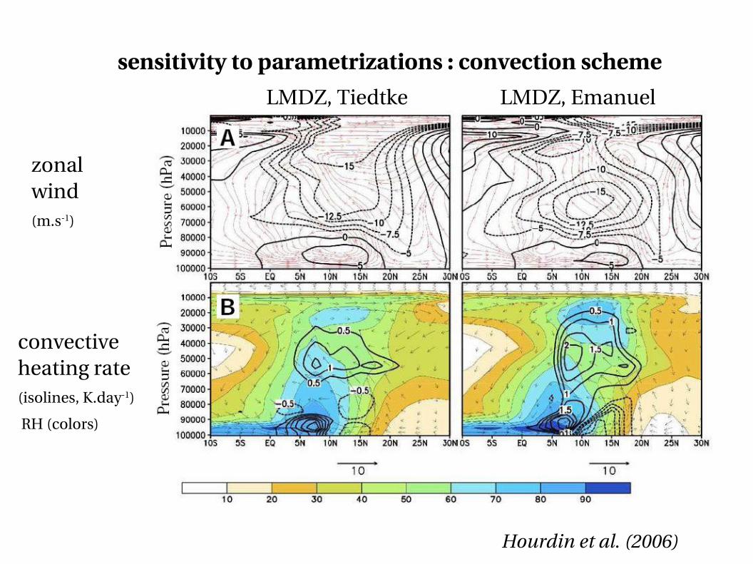
sensitivity to parametrizations : convection scheme

zonal wind(m.s­1)

Hourdin et al. (2006)

convective heating rate(isolines, K.day­1)

 RH (colors)

LMDZ, EmanuelLMDZ, Tiedtke

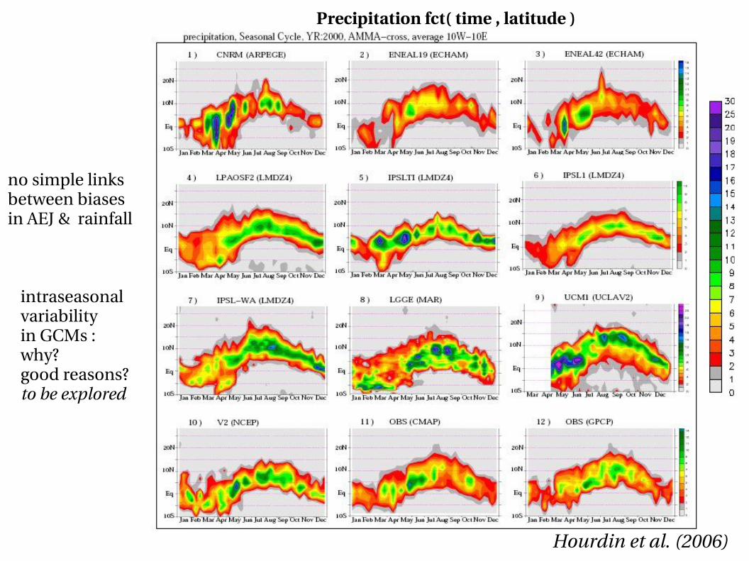
intraseasonal variability in GCMs :why? good reasons?to be explored

no simple linksbetween biases  in AEJ &  rainfall 

Hourdin et al. (2006)

Precipitation fct( time , latitude )

Hourdin et al. (2006)

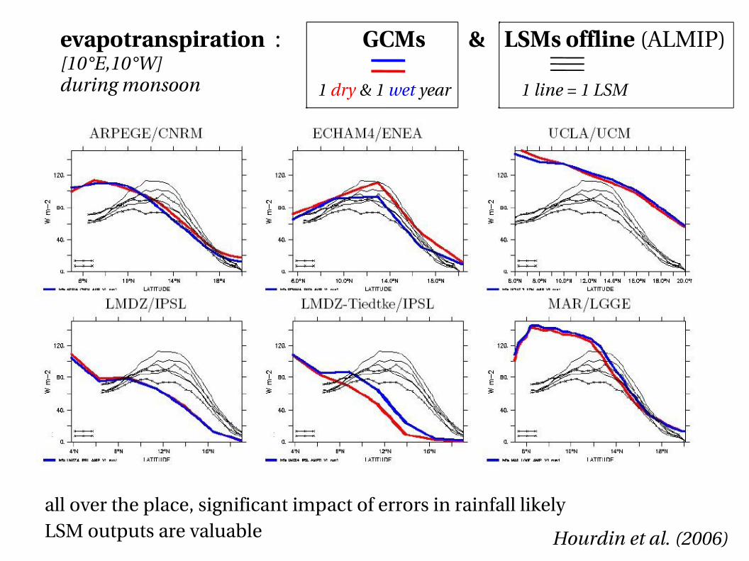
all over the place, significant impact of errors in rainfall likelyLSM outputs are valuable

evapotranspiration  :                GCMs         &    LSMs offline (ALMIP)

1 dry & 1 wet year 1 line = 1 LSM

[10°E,10°W]during monsoon

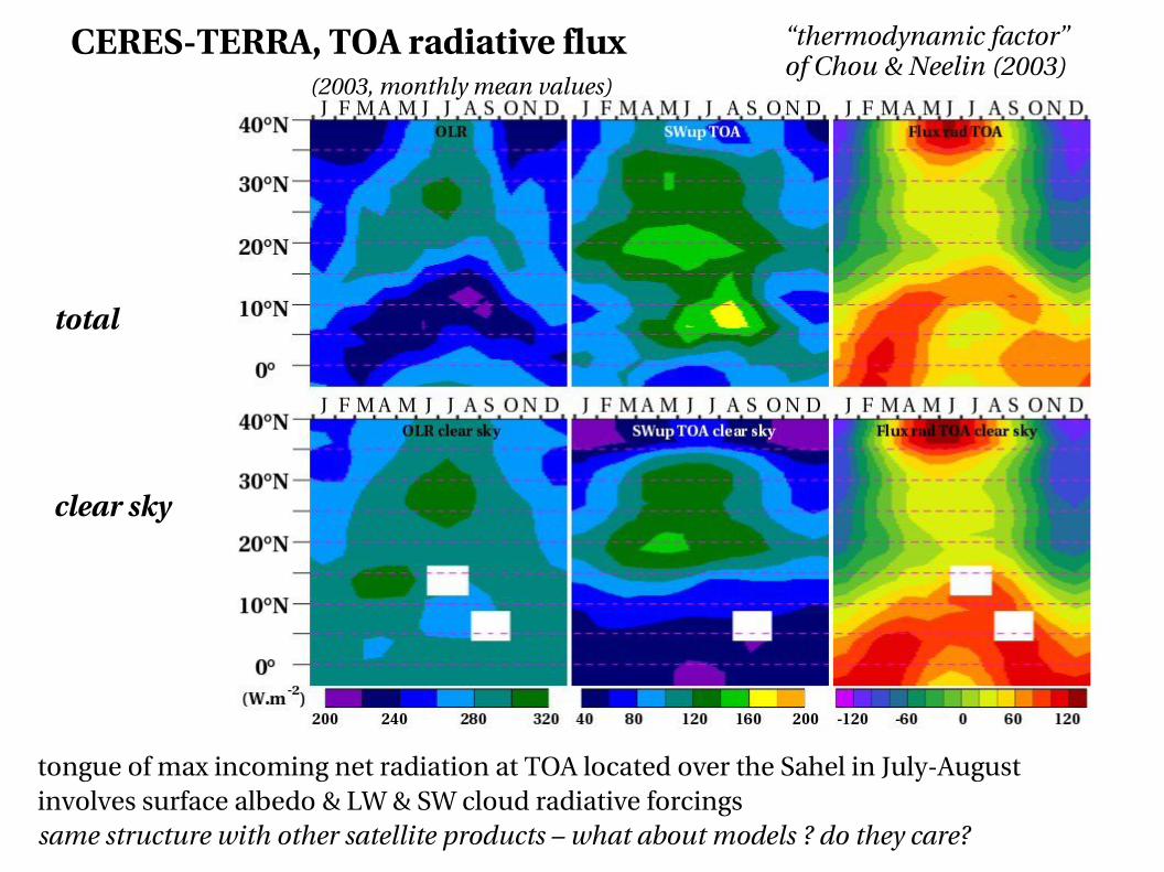
tongue of max incoming net radiation at TOA located over the Sahel in July­Augustinvolves surface albedo & LW & SW cloud radiative forcingssame structure with other satellite products – what about models ? do they care?

CERES­TERRA, TOA radiative flux (2003, monthly mean values)

clear sky

“thermodynamic factor”  of Chou & Neelin (2003) 

total

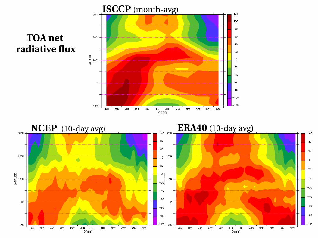
TOA net radiative flux

ISCCP (month­avg)

NCEP  (10­day avg) ERA40 (10­day avg)

OUTLINE

1) broad context

2) modelling 

       • large scale [GCMs along a N­S transect, AMMA­CROSS]

       • mesoscale [comparison of mesoscale simulations of an MCS]

(documenting current state, pointing to specific issues)

3) analysis of data [surface climate and radiative budget)]

• seasonal & diurnal cycle in the Sahel, interannual variability

• contrasting Sahelian & Soudanian sites

(including comparison with ECWMF IFS)

4) summary

mesoscale modelling

until the 90's, much focus was on the simulation of the mature phase of squall lines with CRMs, academic framework, warm/cold bubbles, introduction of ice­phase & radiative processes

Diongue et al. (2002) :  explicit simulation of an observed Sahelian squall linemethod : mesoscale model with grid nesting , inner domain dx=5 km objective : convection­wave interactions in a less academic frame 

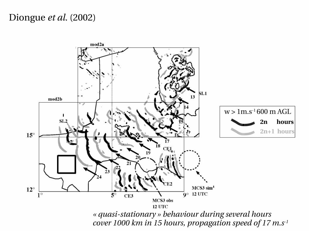
w > 1m.s­1 600 m AGL

2n       hours

2n+1  hours

Diongue et al. (2002) 

« quasi­stationary » behaviour during several hourscover 1000 km in 15 hours, propagation speed of 17 m.s­1

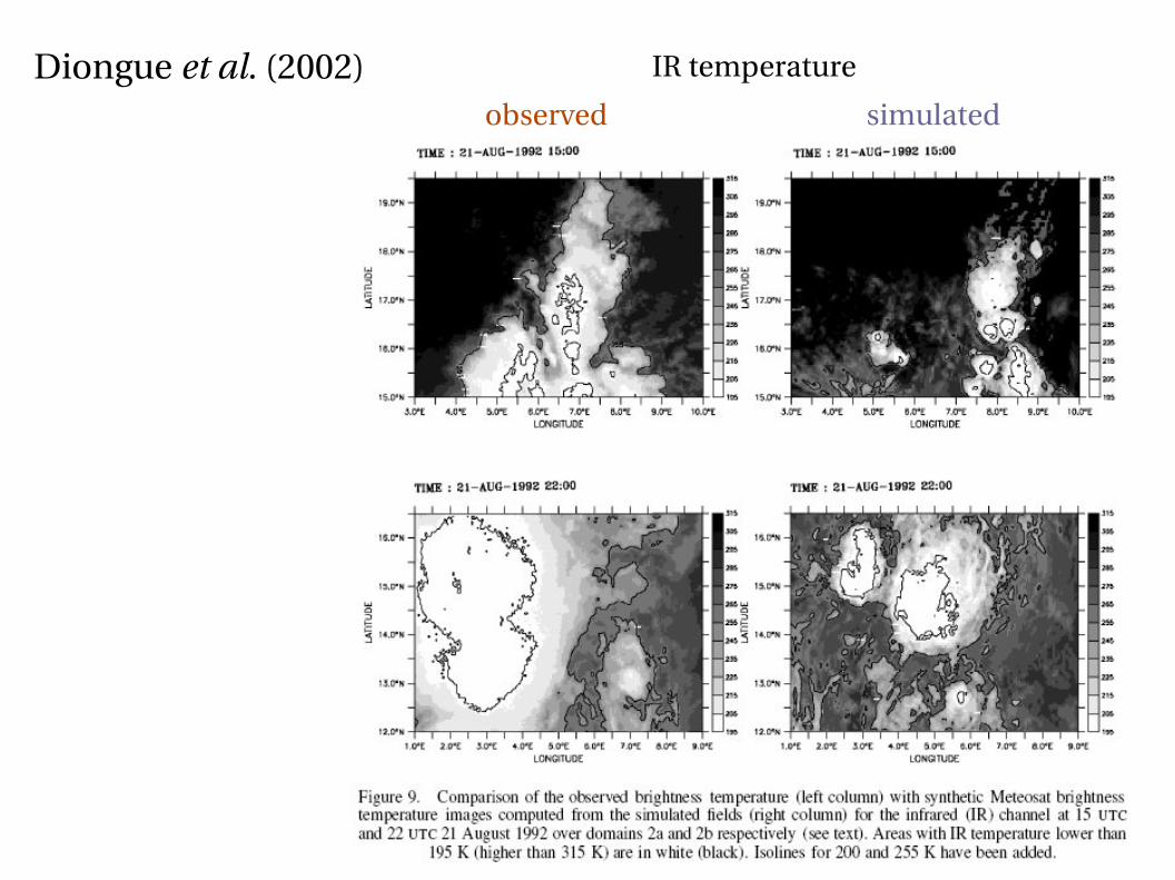
simulatedobserved

Diongue et al. (2002) IR temperature 

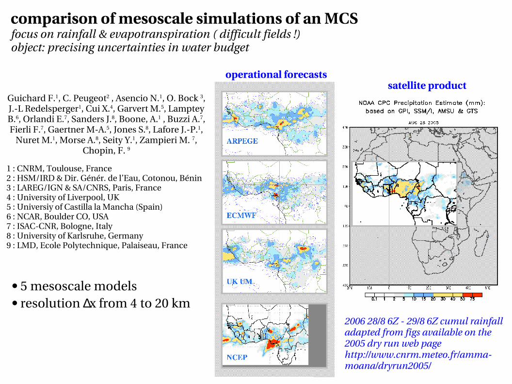
comparison of mesoscale simulations of an MCSfocus on rainfall & evapotranspiration ( difficult fields !) object: precising uncertainties in water budget

Guichard F.1, C. Peugeot2 , Asencio N.1, O. Bock 3, J.­L Redelsperger1, Cui X.4, Garvert M.5, Lamptey B.6, Orlandi E.7, Sanders J.8, Boone, A.1 , Buzzi A.7, Fierli F.7, Gaertner M­A.5, Jones S.8, Lafore J.­P.1, 

Nuret M.1, Morse A.8, Seity Y.1, Zampieri M. 7, Chopin, F. 9

1 : CNRM, Toulouse, France2 : HSM/IRD & Dir. Génér. de l’Eau, Cotonou, Bénin3 : LAREG/IGN & SA/CNRS, Paris, France 4 : University of Liverpool, UK5 : Universiy of Castilla la Mancha (Spain)6 : NCAR, Boulder CO, USA7 : ISAC­CNR, Bologne, Italy8 : University of Karlsruhe, Germany9 : LMD, Ecole Polytechnique, Palaiseau, France 

2006 28/8 6Z ­ 29/8 6Z cumul rainfall adapted from figs available on the 2005 dry run web page http://www.cnrm.meteo.fr/amma­moana/dryrun2005/ 

satellite productoperational forecasts

• 5 mesoscale models• resolution ∆x from 4 to 20 km

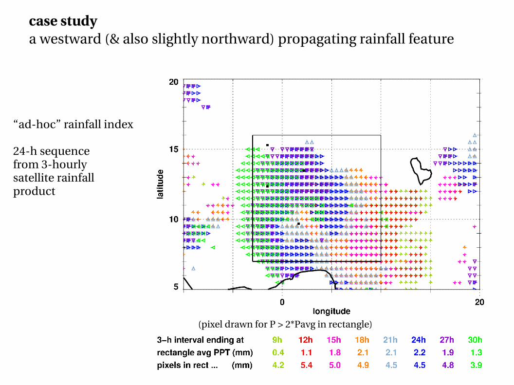
(pixel drawn for P > 2*Pavg in rectangle)

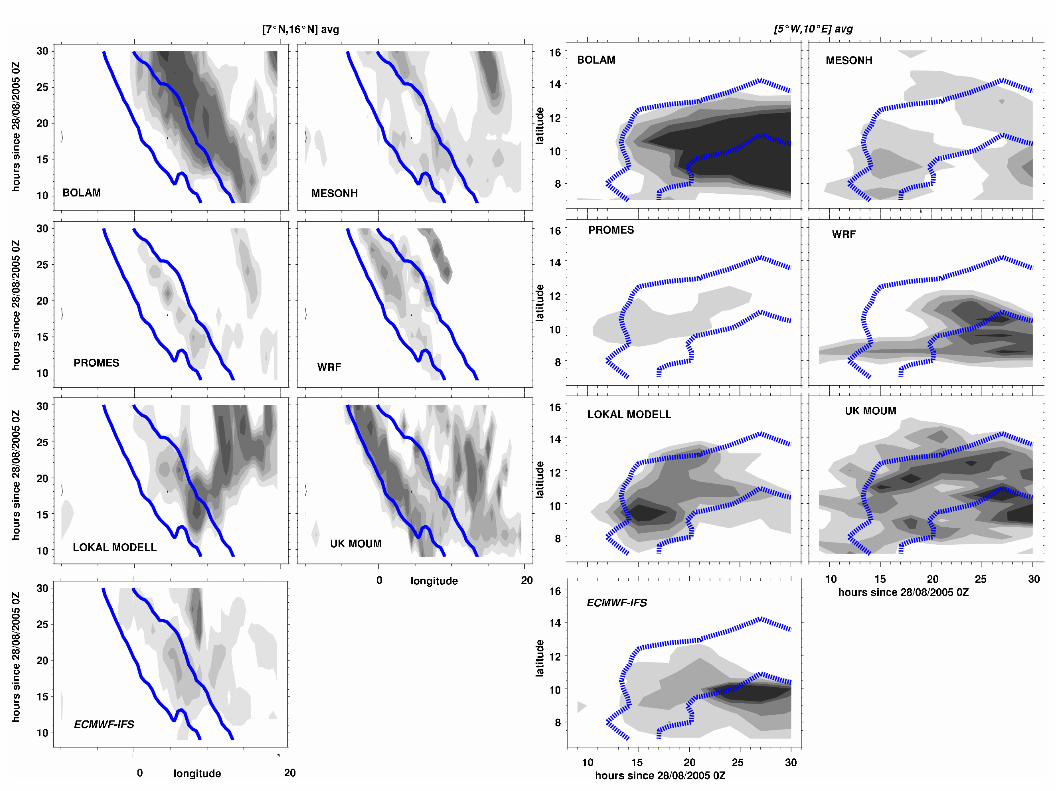
case studya westward (& also slightly northward) propagating rainfall feature  

“ad­hoc” rainfall index 

24­h sequence from 3­hourlysatellite rainfall product

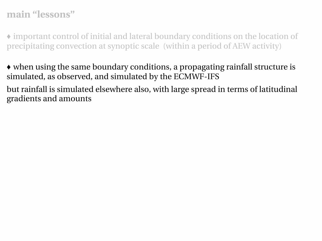
main “lessons”

♦ important control of initial and lateral boundary conditions on the location of precipitating convection at synoptic scale  (within a period of AEW activity)

main “lessons”

♦ important control of initial and lateral boundary conditions on the location of precipitating convection at synoptic scale  (within a period of AEW activity)

♦ when using the same boundary conditions, a propagating rainfall structure is simulated, as observed, and simulated by the ECMWF­IFS 

but rainfall is simulated elsewhere also, with large spread in terms of latitudinal gradients and amounts

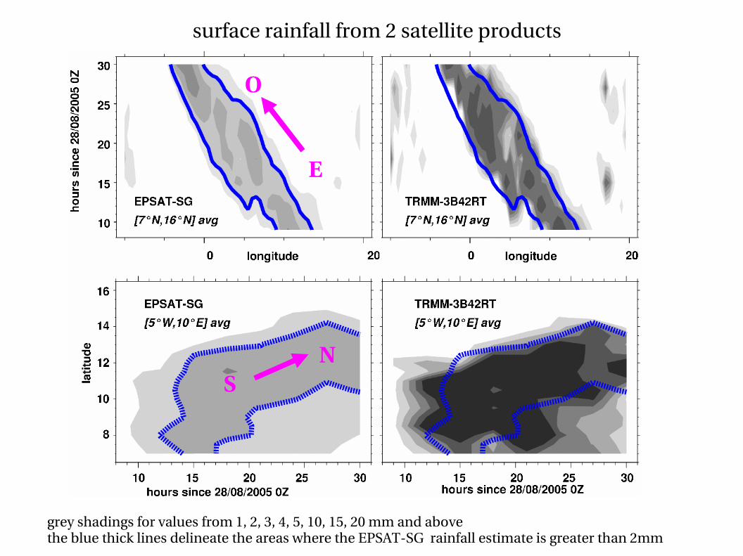
grey shadings for values from 1, 2, 3, 4, 5, 10, 15, 20 mm and above the blue thick lines delineate the areas where the EPSAT­SG  rainfall estimate is greater than 2mm 

O

E

SN

surface rainfall from 2 satellite products

main “lessons”

♦ important control of initial and lateral boundary conditions on the location of precipitating convection at synoptic scale  (within a period of AEW activity)

♦ when using the same boundary conditions, a propagating rainfall structure is simulated, as observed, and simulated by the ECMWF­IFS 

but rainfall is simulated elsewhere also, with large spread in terms of latitudinal gradients and amounts

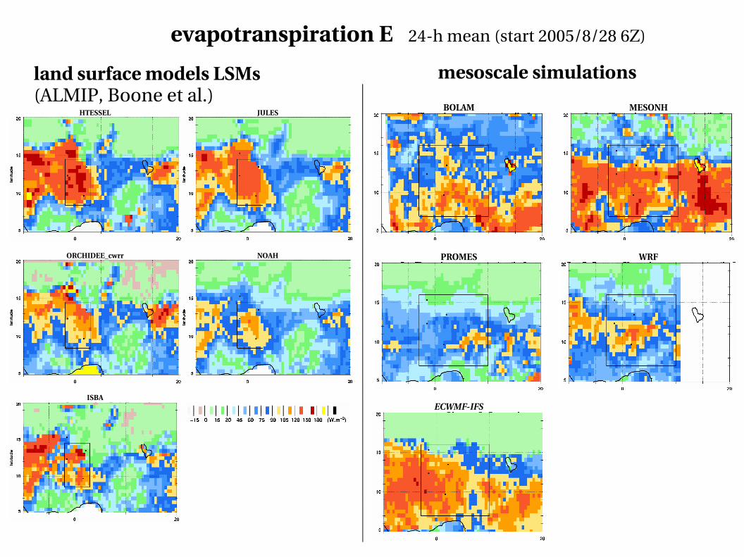
♦ evapotransp. E quite variable among runs (mean & and latitudinal gradient)

but in most simulations structures too zonally symetric / LSM outputs (ALMIP)

HTESSEL JULES

ORCHIDEE_cwrr NOAH

ISBA

BOLAM MESONH

PROMES WRF

ECWMF­IFS

 evapotranspiration E   24­h mean (start 2005/8/28 6Z) 

land surface models LSMs (ALMIP, Boone et al.)

mesoscale simulations

main “lessons”

♦ important control of initial and lateral boundary conditions on the location of precipitating convection at synoptic scale  (within a period of AEW activity)

♦ when using the same boundary conditions, a propagating rainfall structure is simulated, as observed, and simulated by the ECMWF­IFS 

but rainfall is simulated elsewhere also, with large spread in terms of latitudinal gradients and amounts

♦ evapotransp. E quite variable among runs (mean & and latitudinal gradient)but in most simulations structures too zonally symetric / LSM outputs (ALMIP)

♦ the overestimation of  E by MesoNH (& ECMWF­IFS) is related to an overestimation of Rnet, not to an evaporative fraction that would be too high, differences in SWin point to a lack of clouds

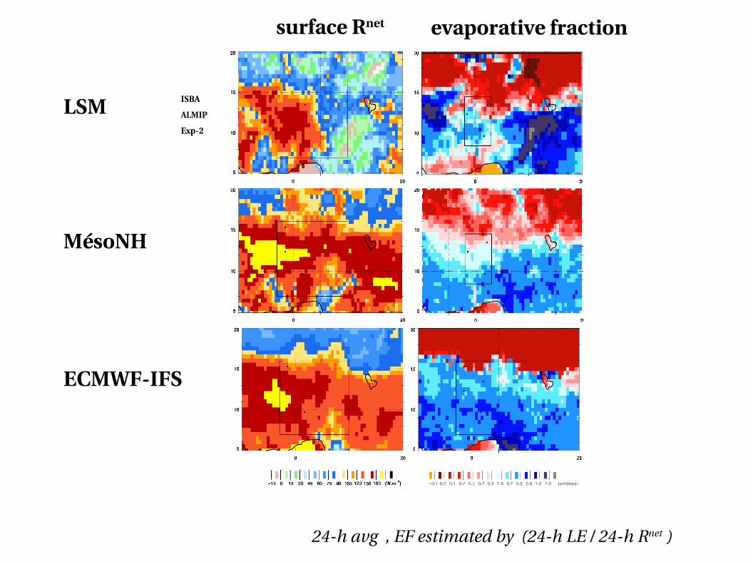
24­h avg  , EF estimated by  (24­h LE / 24­h Rnet )

 

ISBA  

ALMIP

Exp­2

surface Rnet evaporative fraction

LSM

MésoNH

ECMWF­IFS

main “lessons”

♦ important control of initial and lateral boundary conditions on the location of precipitating convection at synoptic scale  (within a period of AEW activity)

♦ when using the same boundary conditions, a propagating rainfall structure is simulated, as observed, and simulated by the ECMWF­IFS 

but rainfall is simulated elsewhere also, with large spread in terms of latitudinal gradients and amounts

♦ evapotransp. E quite variable among runs (mean & and latitudinal gradient)but in all simulations structures too zonally symetric / LSM outputs (ALMIP)

♦ the overestimation of  E by MesoNH (& ECMWF­IFS) is related to an overestimation of Rnet, not to an evaporative fraction that would be too high, differences in SWin point to a lack of clouds

♦ at higher resolution, the partition H , LE is modified (explicit v param convection)    scales of variability & distribution of rainfall along latitude as well, and propagation     is faster 

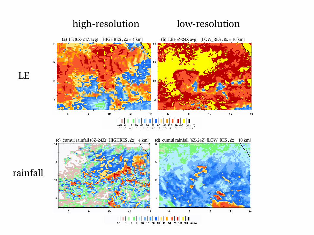
(a)  LE (6Z­24Z avg)   [HIGHRES , ∆x = 4 km] (b)  LE (6Z­24Z avg)   [LOW_RES , ∆x = 10 km]

(c)  cumul rainfall (6Z­24Z) [HIGHRES , ∆x = 4 km] (d)  cumul rainfall (6Z­24Z) [LOW_RES , ∆x = 10 km]

high­resolution low­resolution

LE

rainfall

epilogue

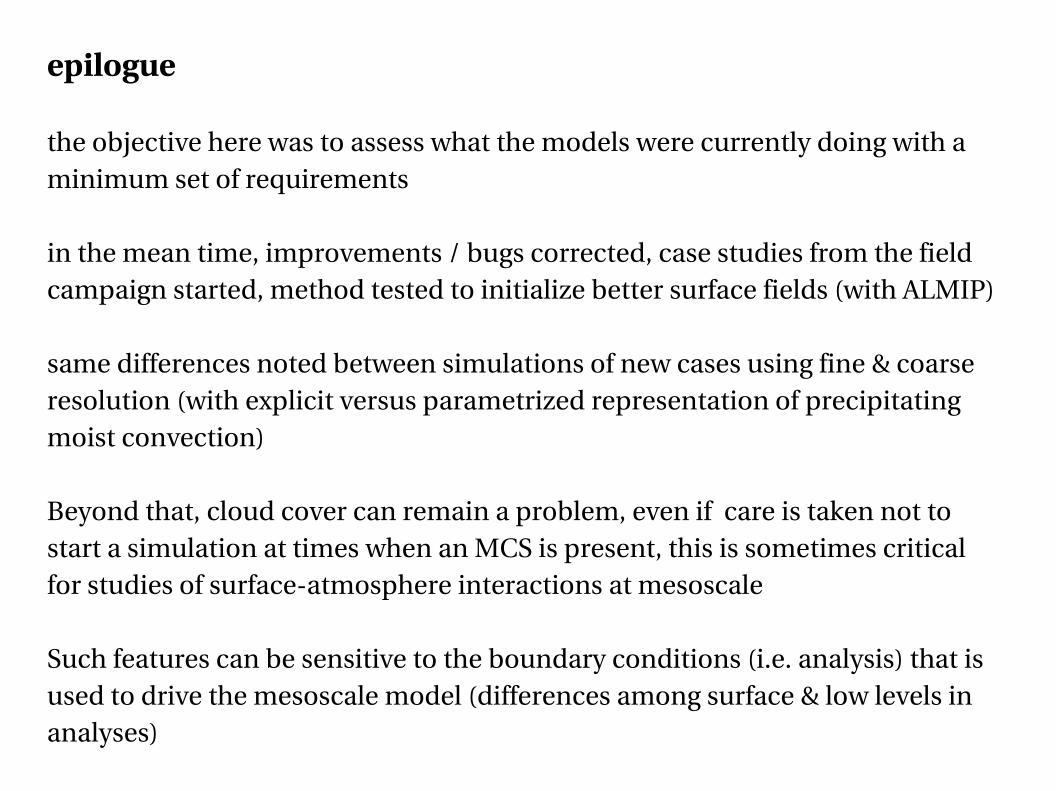
the objective here was to assess what the models were currently doing with a minimum set of requirements 

in the mean time, improvements / bugs corrected, case studies from the field campaign started, method tested to initialize better surface fields (with ALMIP)

same differences noted between simulations of new cases using fine & coarse resolution (with explicit versus parametrized representation of precipitating moist convection)

Beyond that, cloud cover can remain a problem, even if  care is taken not to start a simulation at times when an MCS is present, this is sometimes critical for studies of surface­atmosphere interactions at mesoscale

Such features can be sensitive to the boundary conditions (i.e. analysis) that is used to drive the mesoscale model (differences among surface & low levels in analyses)

OUTLINE

1) broad context

2) modelling 

       • large scale [GCMs along a N­S transect, AMMA­CROSS]

       • mesoscale [comparison of mesoscale simulations of an MCS]

(documenting current state, pointing to specific issues)

3) analysis of data [surface climate and radiative budget)]

• seasonal & diurnal cycle in the Sahel, interannual variability

• contrasting Sahelian & Soudanian sites

(including comparison with ECWMF IFS)

4) summary

surface radiative budget & thermodynamics in the Sahel 

♦  data for guiding modelling, testing the realism of proposed mechanisms      & coupling , precise quantification in time and space

• which factors control surface radiative fluxes and their variations?• which relationships  between  θe , fluxes & precipitation?

• precising magnitude & nature of interannual variability

• characterizing differences with more Southern sites (meridional gradient) 

♦  such types of analyses: conducted over other land regions     (e.g. Betts & Ball 1998)

♦  data types & sources :• automatic weather station, T, RH, wind, radiative fluxes, pressure• sunphotometer Aeronet : aerosol optical thickness , precipitable water

Mougin, Timouk et al. (Sahelian zone, Gourma, 15°N to 17°N)  Galle, Lloyd et al. (Soudanian zone, Oueme basin, ~10°N)

• high­resolution soundings (Niamey 13°N, AMMA SOP, Parker et al. (2008))

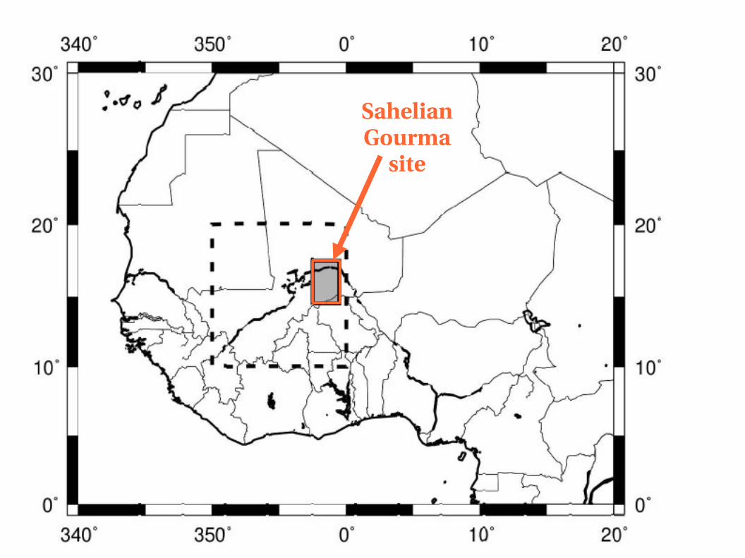
SahelianGourma

site

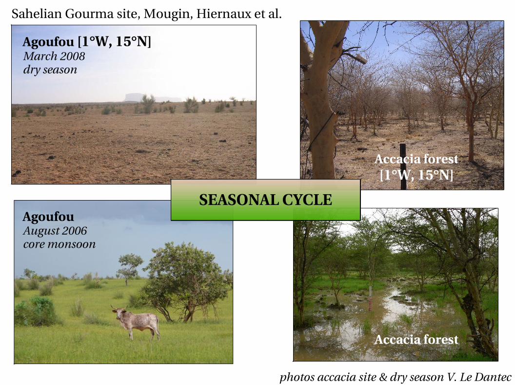
photos accacia site & dry season V. Le Dantec

SEASONAL CYCLE

Sahelian Gourma site, Mougin, Hiernaux et al. 

Agoufou [1°W, 15°N]March 2008dry season

AgoufouAugust 2006core monsoon

Accacia forest[1°W, 15°N]

Accacia forest

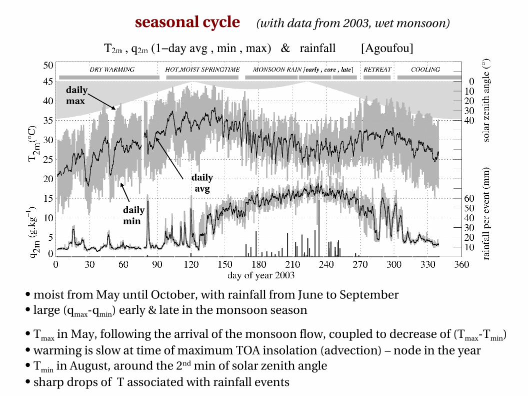
seasonal cycle     (with data from 2003, wet monsoon)

• moist from May until October, with rainfall from June to September• large (qmax­qmin) early & late in the monsoon season

• Tmax in May, following the arrival of the monsoon flow, coupled to decrease of (Tmax­Tmin)• warming is slow at time of maximum TOA insolation (advection) – node in the year   • Tmin in August, around the 2nd min of solar zenith angle• sharp drops of  T associated with rainfall events

dailymax

daily min

daily avg

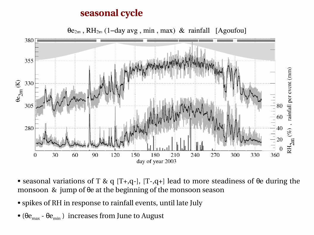
• seasonal variations of T & q [T+,q­],  [T­,q+]  lead to more steadiness of θe during the monsoon  &  jump of θe at the beginning of the monsoon season

• spikes of RH in response to rainfall events, until late July

• (θemax ­ θemin )  increases from June to August 

seasonal cycle     

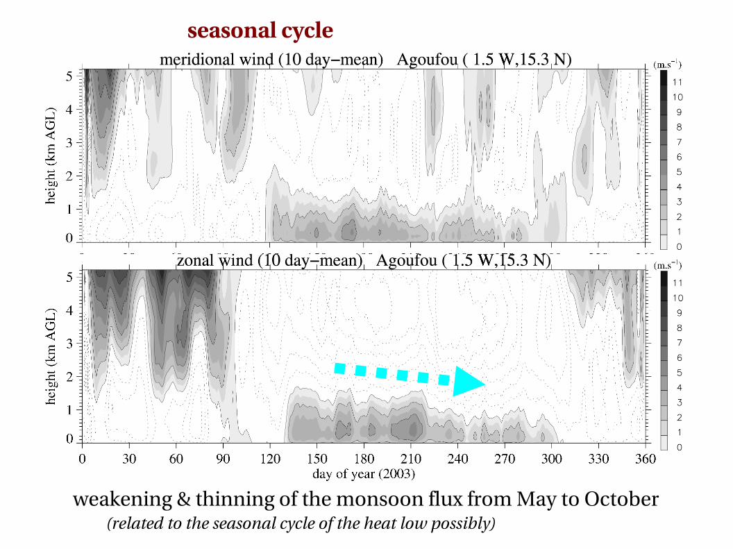
seasonal cycle     

weakening & thinning of the monsoon flux from May to October (related to the seasonal cycle of the heat low possibly) 

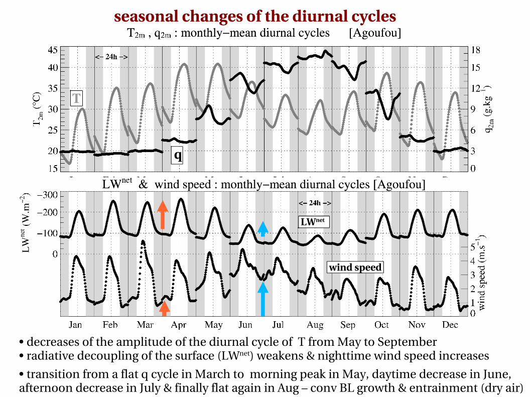
seasonal changes of the diurnal cycles  

• decreases of the amplitude of the diurnal cycle of  T from May to September• radiative decoupling of the surface (LWnet) weakens & nighttime wind speed increases

• transition from a flat q cycle in March to  morning peak in May, daytime decrease in June, afternoon decrease in July & finally flat again in Aug – conv BL growth & entrainment (dry air)

 wind speed

 q

T

 LWnet

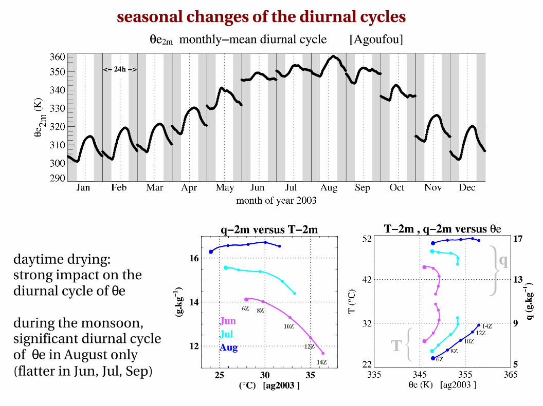
seasonal changes of the diurnal cycles  

daytime drying: strong impact on the diurnal cycle of θe 

during the monsoon, significant diurnal cycleof  θe in August only(flatter in Jun, Jul, Sep)

q

T{

{

(Niamey soundings)~ 30 soundings per monthly­hourly mean profile

For same magnitudes of wind speed (as in this case/example) • when dry (March), stronger surface decoupling: lower nocturnal jet & stable layer

• when moist (May), lower surface decoupling: more mixing & stable layer higher

implies changes on subsequent daytime BL growth

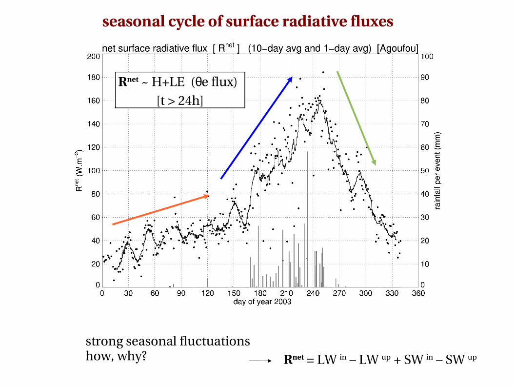
seasonal cycle of surface radiative fluxes  

 Rnet = LW in – LW up + SW in – SW up strong seasonal fluctuationshow, why?

 Rnet ~ H+LE  (θe flux) 

[t > 24h]

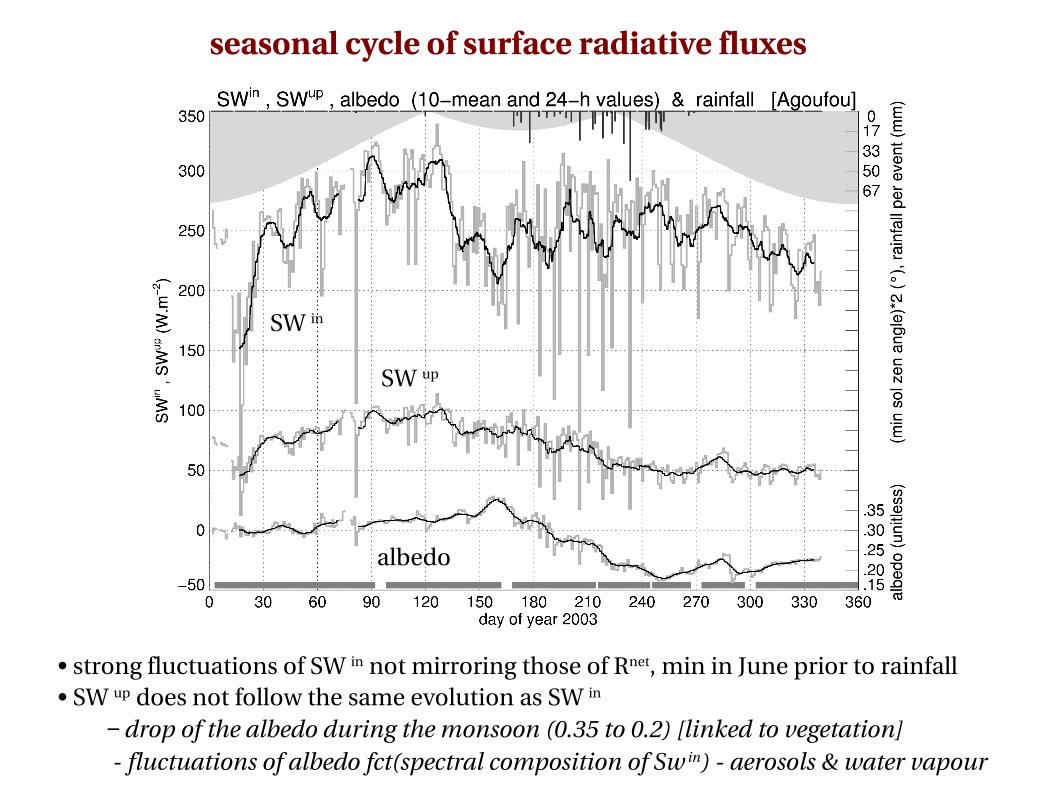
• strong fluctuations of SW in not mirroring those of Rnet, min in June prior to rainfall• SW up does not follow the same evolution as SW in

         − drop of the albedo during the monsoon (0.35 to 0.2) [linked to vegetation]           ­ fluctuations of albedo fct(spectral composition of Sw in) ­ aerosols & water vapour

seasonal cycle of surface radiative fluxes  

SW in

SW up

albedo

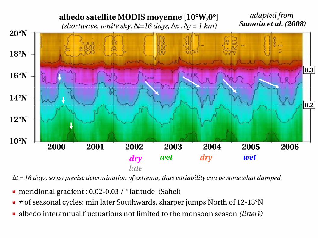
∆t = 16 days, so no precise determination of extrema, thus variability can be somewhat damped

  meridional gradient : 0.02­0.03 / ° latitude  (Sahel)

≠ of seasonal cycles: min later Southwards, sharper jumps North of 12­13°N 

  albedo interannual fluctuations not limited to the monsoon season (litter?)

20°N

albedo satellite MODIS moyenne [10°W,0°](shortwave, white sky, ∆t=16 days, ∆x , ∆y = 1 km)

adapted from Samain et al. (2008)

2002 2003 2004 2005 20062001200010°N

12°N

14°N

16°N

18°N

 wet wetlate

 drydry

 0.3 

 0.2 

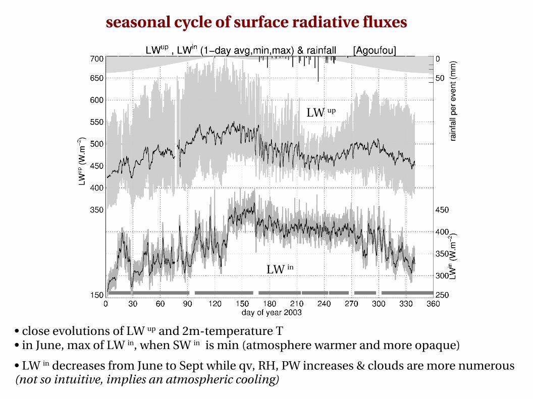
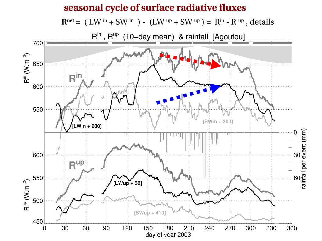
• close evolutions of LW up and 2m­temperature T • in June, max of LW in, when SW in  is min (atmosphere warmer and more opaque)

• LW in decreases from June to Sept while qv, RH, PW increases & clouds are more numerous(not so intuitive, implies an atmospheric cooling)

seasonal cycle of surface radiative fluxes  

LW up

LW in

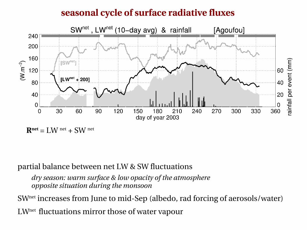
seasonal cycle of surface radiative fluxes  

partial balance between net LW & SW fluctuationsdry season: warm surface & low opacity of the atmosphereopposite situation during the monsoon

SWnet increases from June to mid­Sep (albedo, rad forcing of aerosols/water)

LWnet  fluctuations mirror those of water vapour

 Rnet = LW net + SW net 

 

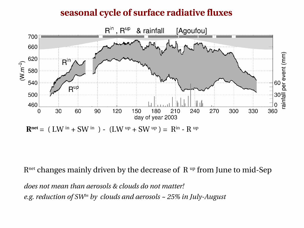
Rnet changes mainly driven by the decrease of  R up from June to mid­Sep

does not mean than aerosols & clouds do not matter!

e.g. reduction of SWin by  clouds and aerosols ~ 25% in July­August

seasonal cycle of surface radiative fluxes  

 Rnet =  ( LW in + SW in   ) ­  (LW up + SW up ) =  Rin ­ R up 

seasonal cycle of surface radiative fluxes  

Rnet =  ( LW in + SW in   ) ­  (LW up + SW up ) =  Rin ­ R up , details

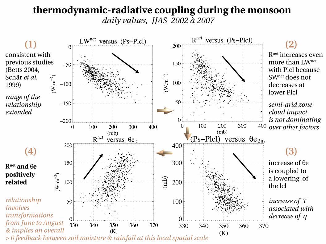
daily values,  JJAS  2002 à 2007 thermodynamic­radiative coupling during the monsoon

consistent with  previous studies (Betts 2004, Schär et al. 1999)

range of the relationship extended

Rnet increases even more than LWnet  with Plcl because SWnet does not decreases at lower Plcl 

semi­arid zonecloud impact is not dominatingover other factors

(1) (2)

increase of θe  is coupled to  a lowering  of the lcl 

increase of  T associated with decrease of  q

(3)Rnet and θe positively related

relationship involves transformations from June to August& implies an overall> 0 feedback between soil moisture & rainfall at this local spatial scale

(4)

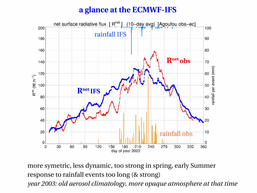
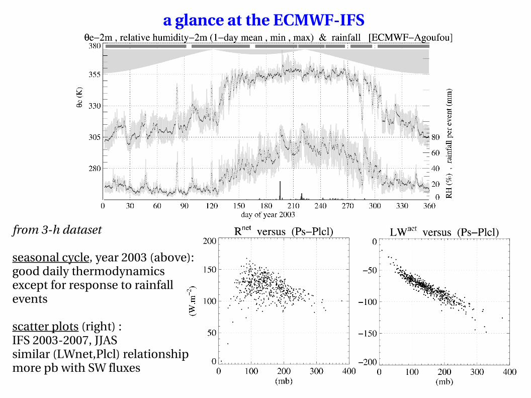
a glance at the ECMWF­IFS

more symetric, less dynamic, too strong in spring, early Summerresponse to rainfall events too long (& strong) year 2003: old aerosol climatology, more opaque atmosphere at that time

Rnet obs

Rnet IFS

rainfall IFS

rainfall obs

a glance at the ECMWF­IFS

from 3­h dataset

seasonal cycle, year 2003 (above): good daily thermodynamicsexcept for response to rainfall events

scatter plots (right) :IFS 2003­2007, JJASsimilar (LWnet,Plcl) relationshipmore pb with SW fluxes

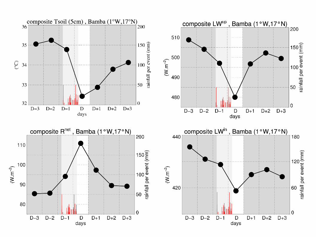
INTERANNUAL VARIABILITY

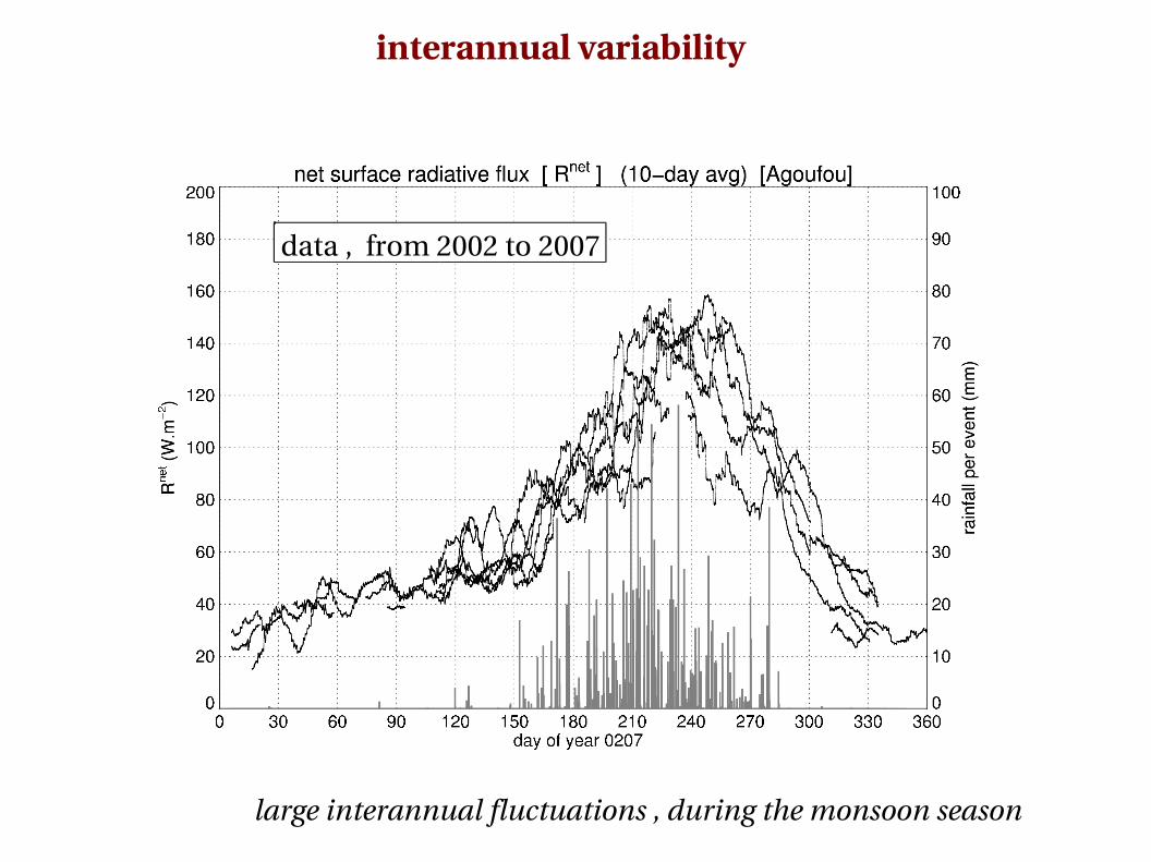
interannual variability

 data ,  from 2002 to 2007 

large interannual fluctuations , during the monsoon season

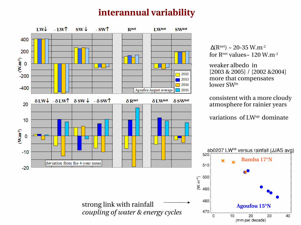
∆(Rnet) ~ 20­35 W.m­2

for Rnet values~ 120 W.m­2

weaker albedo  in [2003 & 2005] / [2002 &2004] more that compensates lower SWin 

consistent with a more cloudy atmosphere for rainier years

variations  of LWup  dominate

interannual variability

strong link with rainfallcoupling of water & energy cycles

Agoufou 15°N

Bamba 17°N

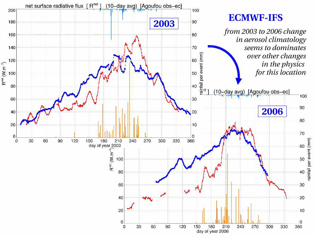
ECMWF­IFS2003

2006

from 2003 to 2006 change in aerosol climatology 

seems to dominates over other changes 

in the physics  for this location 

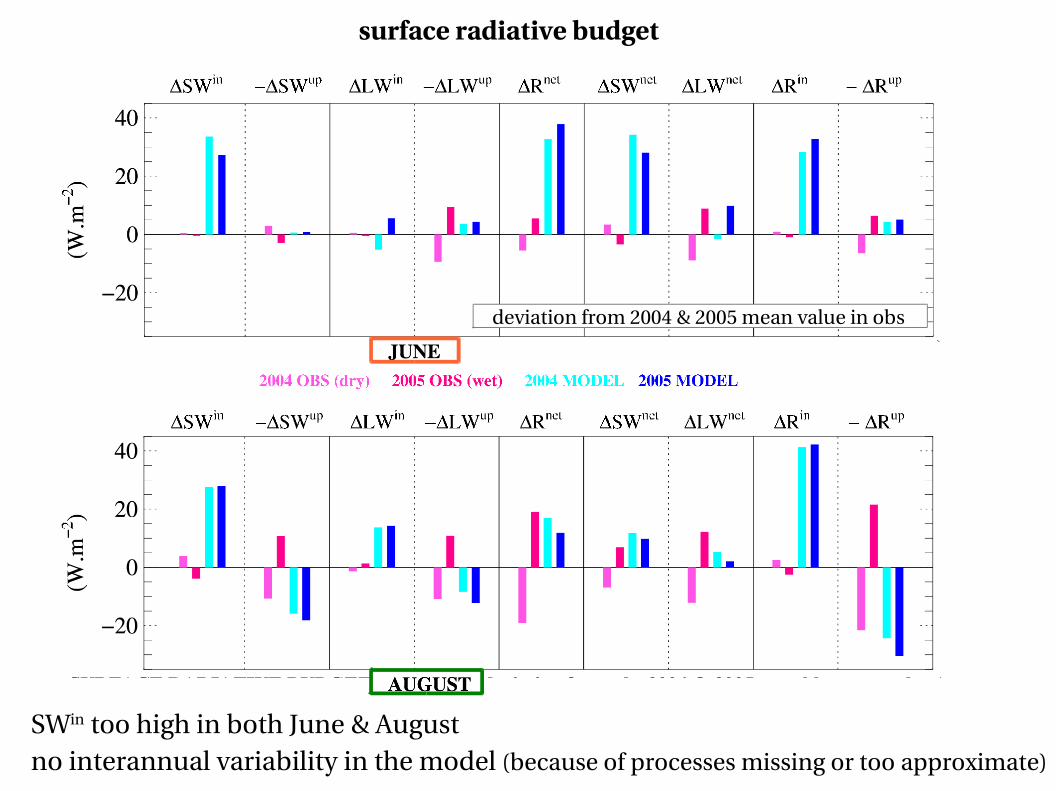
surface radiative budget

SWin too high in both June & Augustno interannual variability in the model (because of processes missing or too approximate) 

 deviation from 2004 & 2005 mean value in obs 

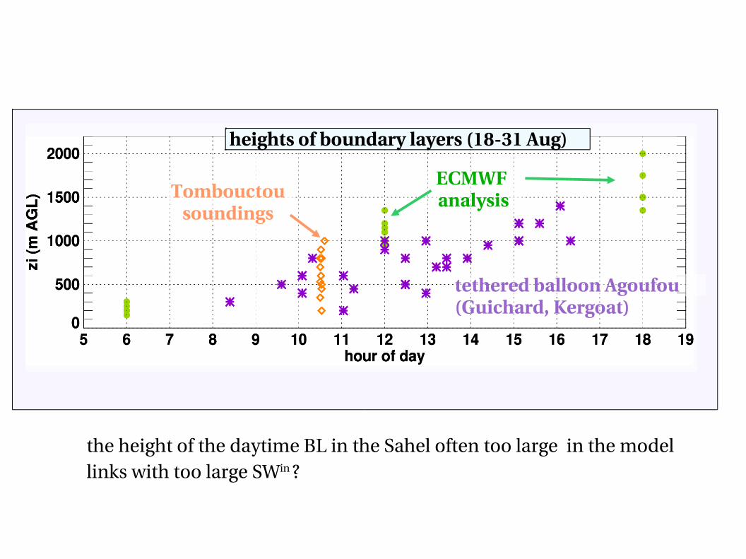
Tombouctou soundings 

ECMWF analysis

tethered balloon Agoufou (Guichard, Kergoat)

 heights of boundary layers (18­31 Aug)

the height of the daytime BL in the Sahel often too large  in the modellinks with too large SWin ?

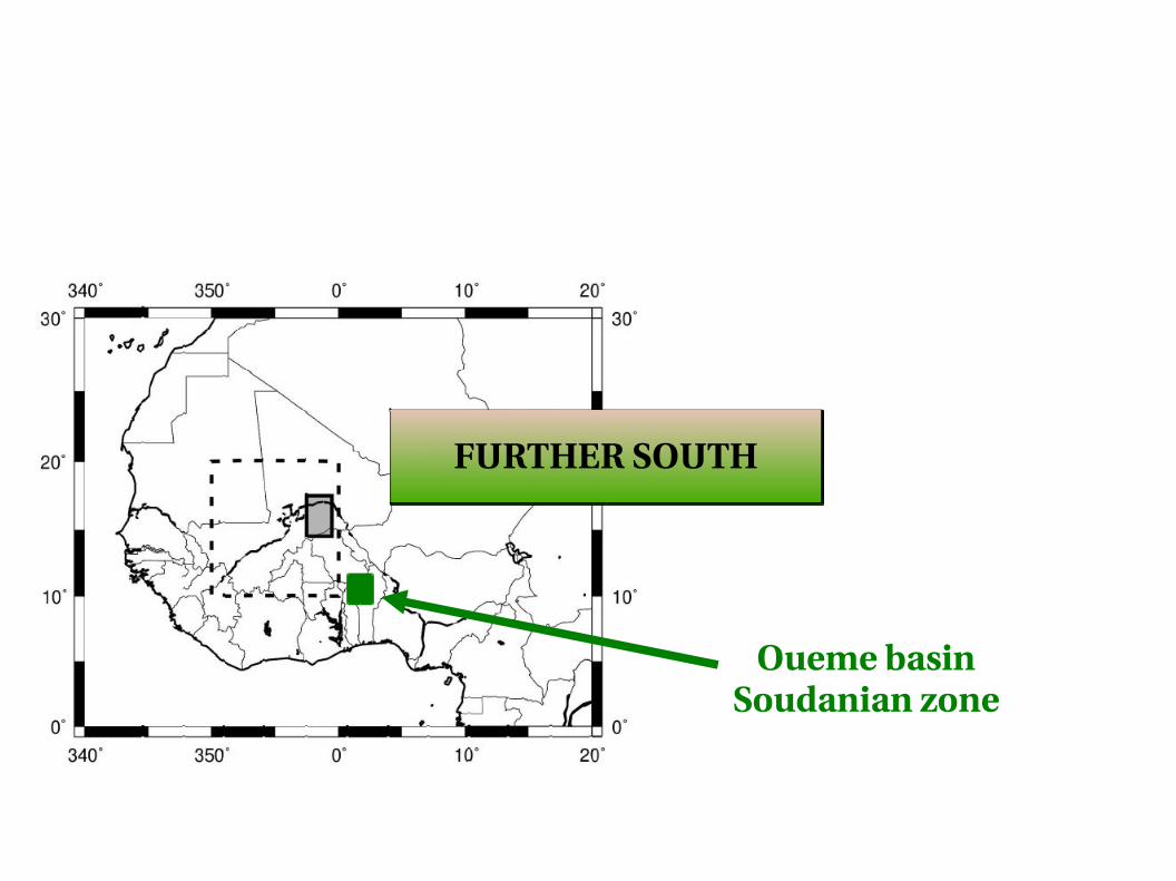
FURTHER SOUTH

Oueme basinSoudanian zone

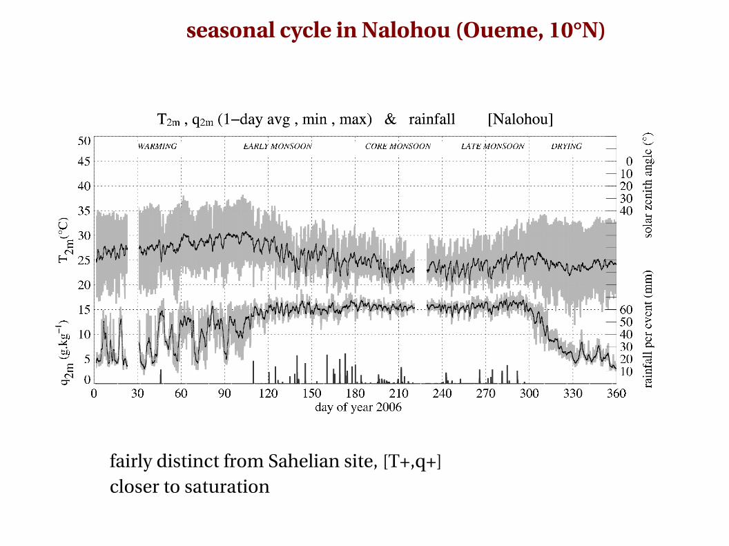
seasonal cycle in Nalohou (Oueme, 10°N)     

fairly distinct from Sahelian site, [T+,q+]closer to saturation

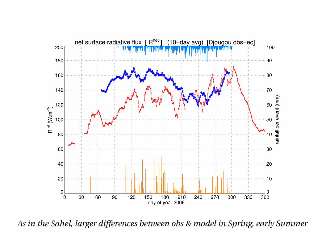
As in the Sahel, larger differences between obs & model in Spring, early Summer

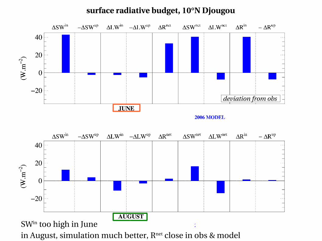
surface radiative budget, 10°N Djougou

deviation from obs

SWin too high in Junein August, simulation much better, Rnet close in obs & model

RAINFALL EVENT COMPOSITE

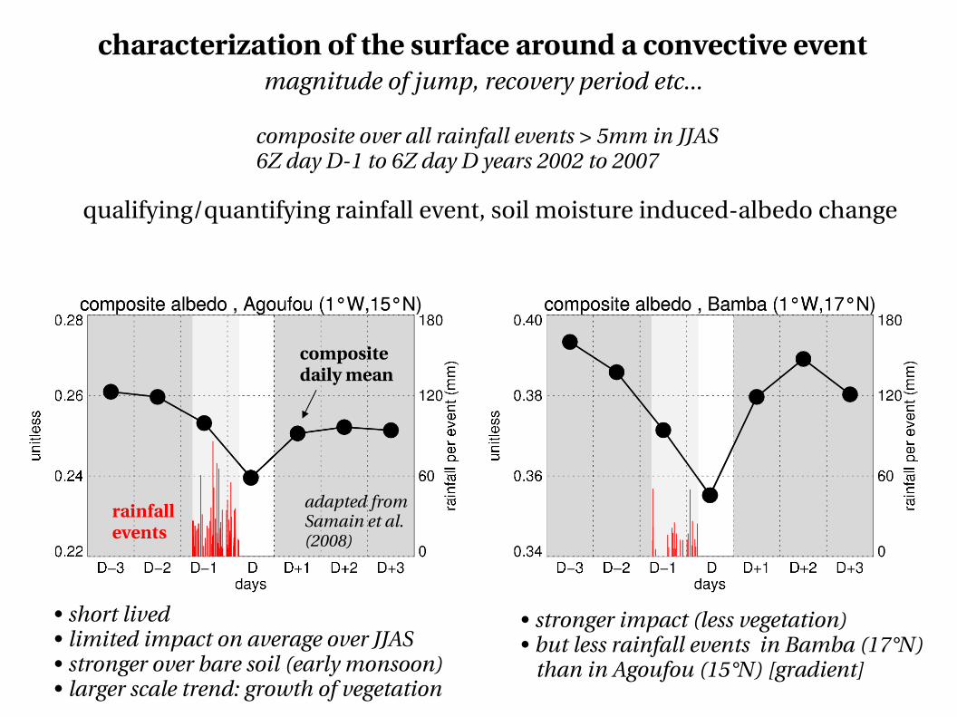
characterization of the surface around a convective eventmagnitude of jump, recovery period etc...

qualifying/quantifying rainfall event, soil moisture induced­albedo change

adapted from Samain et al. (2008)

• short lived• limited impact on average over JJAS• stronger over bare soil (early monsoon)• larger scale trend: growth of vegetation

composite over all rainfall events > 5mm in JJAS  6Z day D­1 to 6Z day D years 2002 to 2007

• stronger impact (less vegetation)• but less rainfall events  in Bamba (17°N)    than in Agoufou (15°N) [gradient]  

rainfall events

composite daily mean

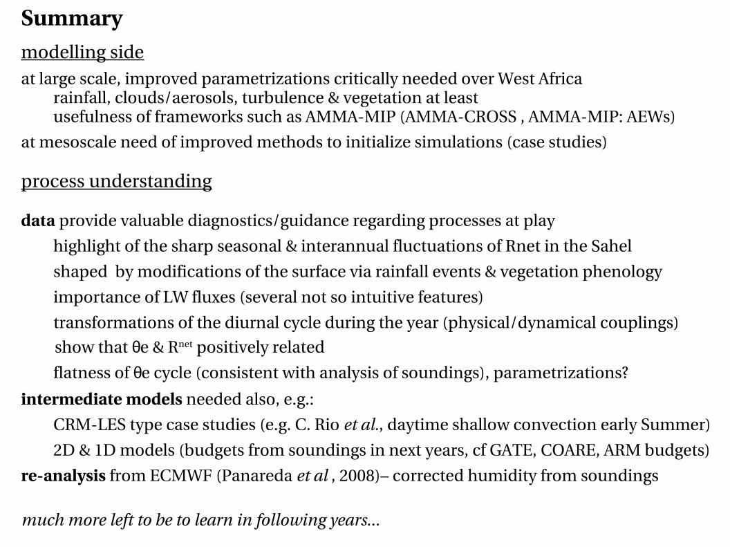
Summary

modelling sideat large scale, improved parametrizations critically needed over West Africa

rainfall, clouds/aerosols, turbulence & vegetation at leastusefulness of frameworks such as AMMA­MIP (AMMA­CROSS , AMMA­MIP: AEWs)

at mesoscale need of improved methods to initialize simulations (case studies)

process understanding 

data provide valuable diagnostics/guidance regarding processes at play

highlight of the sharp seasonal & interannual fluctuations of Rnet in the Sahel  

shaped  by modifications of the surface via rainfall events & vegetation phenology 

importance of LW fluxes (several not so intuitive features) 

transformations of the diurnal cycle during the year (physical/dynamical couplings)

         show that θe & Rnet positively related

flatness of θe cycle (consistent with analysis of soundings), parametrizations?

intermediate models needed also, e.g.:

CRM­LES type case studies (e.g. C. Rio et al., daytime shallow convection early Summer)

2D & 1D models (budgets from soundings in next years, cf GATE, COARE, ARM budgets)

re­analysis from ECMWF (Panareda et al , 2008)– corrected humidity from soundings

much more left to be to learn in following years... 

Thank you