Embed Size (px)
Citation preview

Colloidal Interactions in Solutions
Yun Liu
National Institute of Standards and Technology (NIST) Center for Neutron Research
Department of Materials Science and EngineeringUniversity of Maryland, College Park
Tutorial Session, ACNS, 2008, Santa Fe
Outline
1.
Introduction2.
Contrast term
3.
Form factor P(Q)4.
Structure factor S(Q)
5.
Colloidal interactions6.
Calculate structure factor S(Q)
7.
Examples8.
Relations with some other methods
9.
Summary
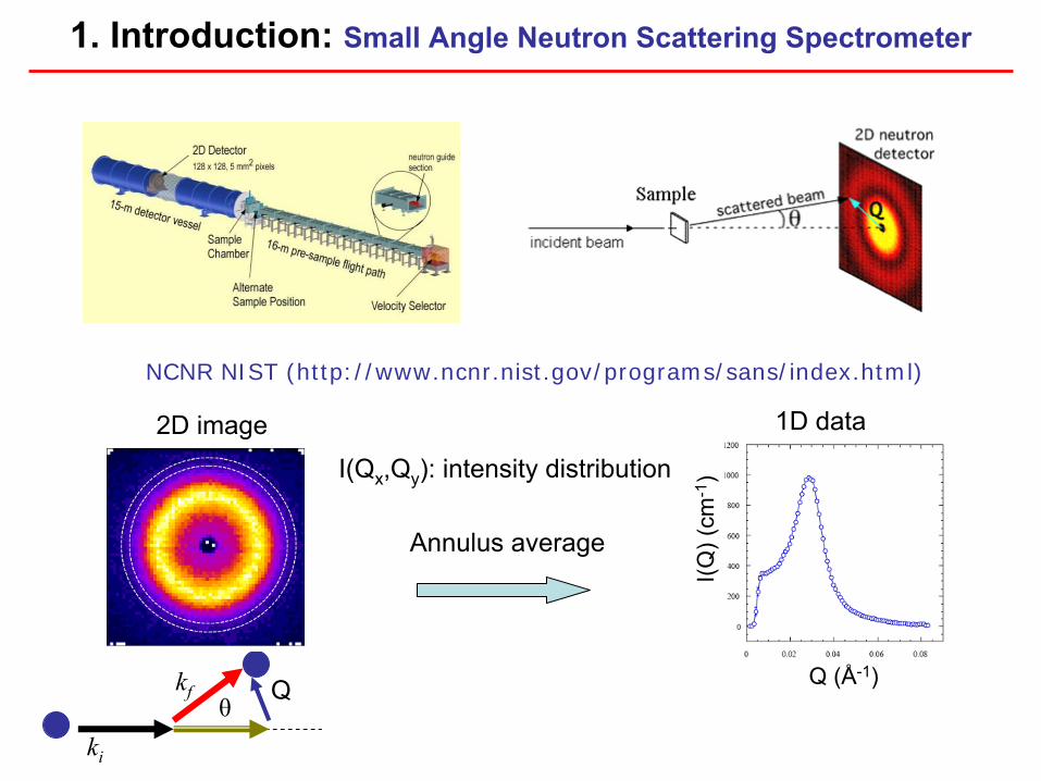
1. Introduction: Small Angle Neutron Scattering Spectrometer
NCNR NIST (http://www.ncnr.nist.gov/programs/sans/index.html)
ki
kfθ
Q
1D data
I(Q) (
cm-1
)Q (Å-1)
Annulus average
2D image
I(Qx
,Qy
): intensity distribution
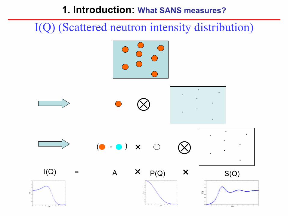
I(Q) (Scattered neutron intensity distribution)
⊗
⊗-( ) ×
I(Q) = A P(Q)× S(Q)×
1. Introduction: What SANS measures?
I(Q) = A ×
P(Q) ×
S(Q)
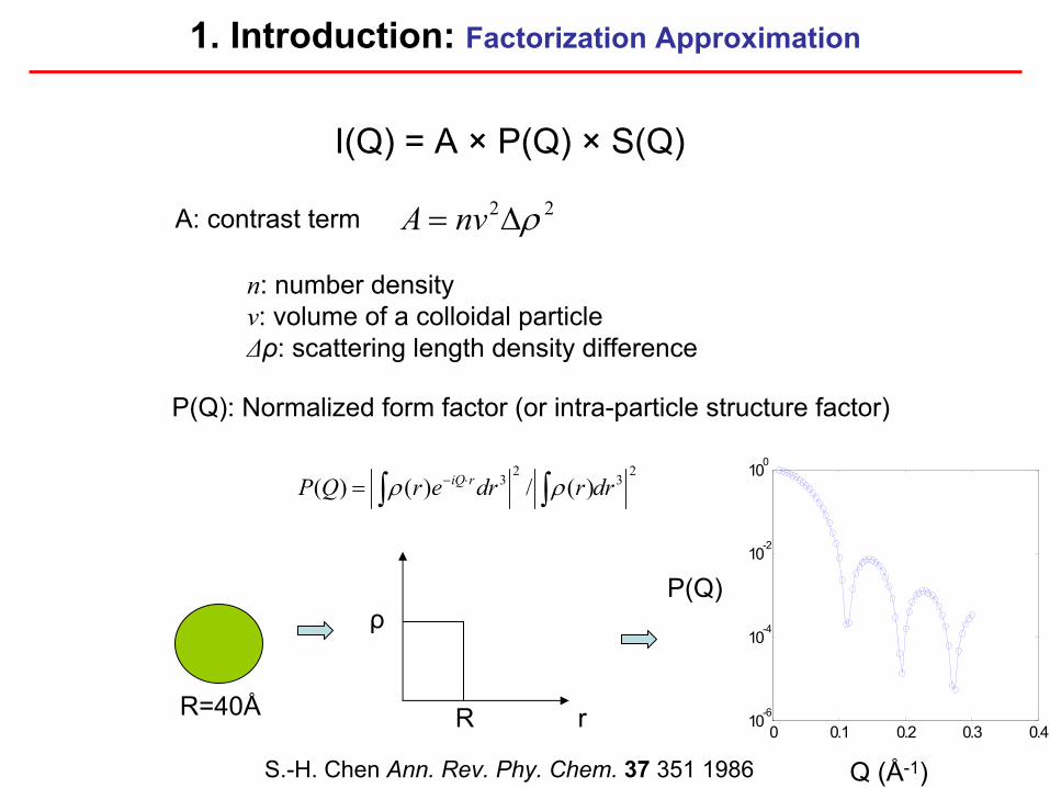
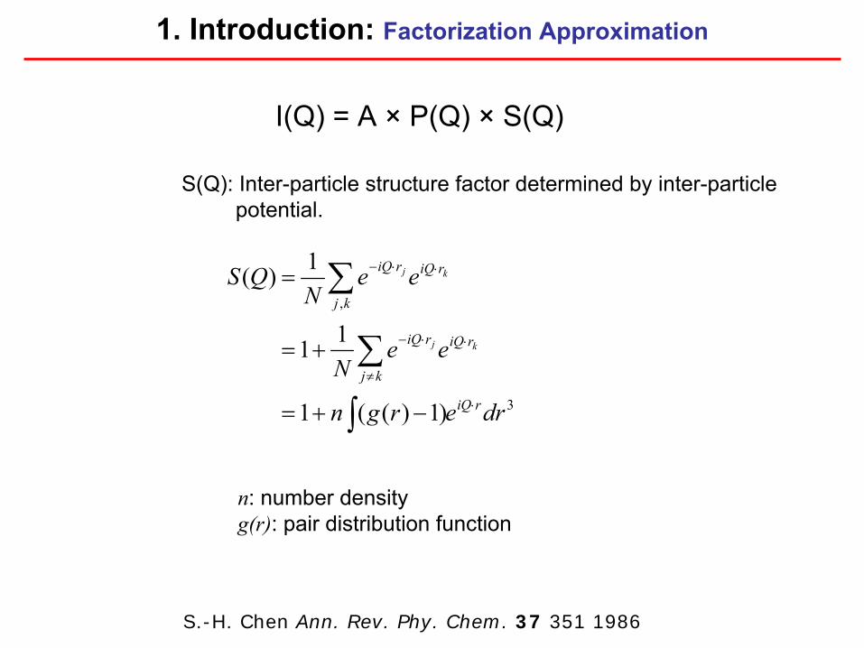
1. Introduction: Factorization Approximation
S.-H. Chen Ann. Rev. Phy. Chem.
37
351 1986
A: contrast term 22 ρΔ= nvA
n: number density v: volume of a colloidal particleΔρ: scattering length density difference
23
23 )(/)()( drrdrerQP riQ ∫∫ ⋅−= ρρ
P(Q): Normalized form factor (or intra-particle structure factor)
R=40Å rR
ρ
0 0.1 0.2 0.3 0.410-6
10-4
10-2
100
P(Q)
Q (Å-1)
I(Q) = A ×
P(Q) ×
S(Q)
1. Introduction: Factorization Approximation
S.-H. Chen Ann. Rev. Phy. Chem. 37 351 1986
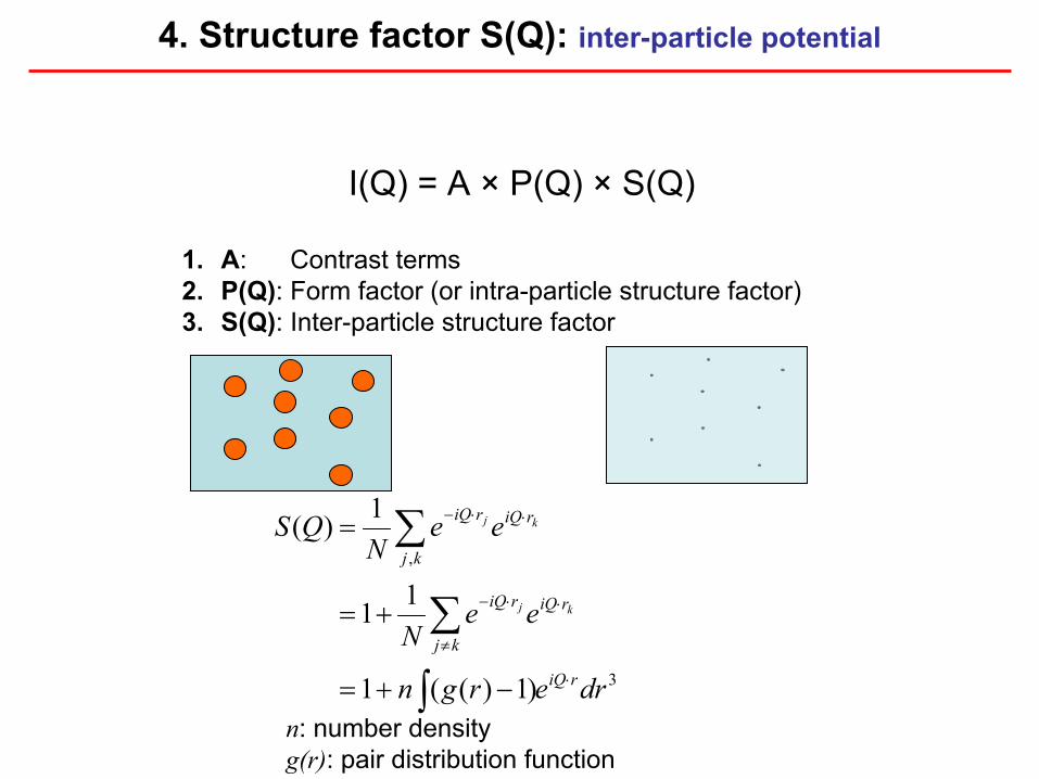
S(Q): Inter-particle structure factor determined by inter-particlepotential.
3
,
)1)((1
11
1)(
drergn
eeN
eeN
QS
riQ
kj
riQriQ
kj
riQriQ
kj
kj
⋅
≠
⋅⋅−
⋅⋅−
∫
∑
∑
−+=
+=
=
n: number densityg(r): pair distribution function
I(Q) = A ×
P(Q) ×
S(Q)
1.
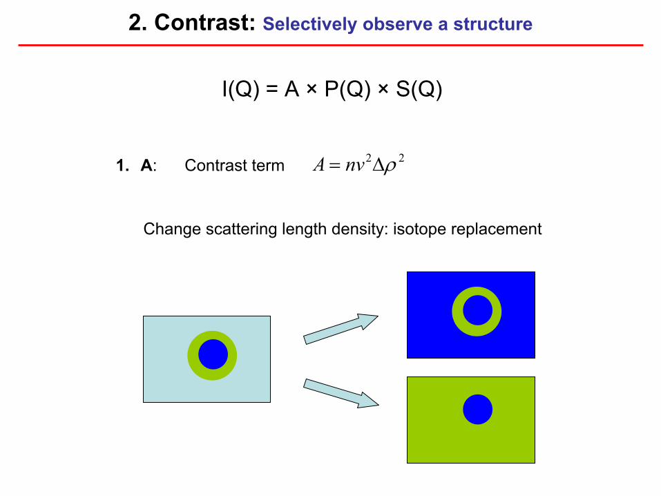
A: Contrast term
Change scattering length density: isotope replacement
2. Contrast: Selectively observe a structure
22 ρΔ= nvA
I(Q) = A ×
P(Q) ×
S(Q)
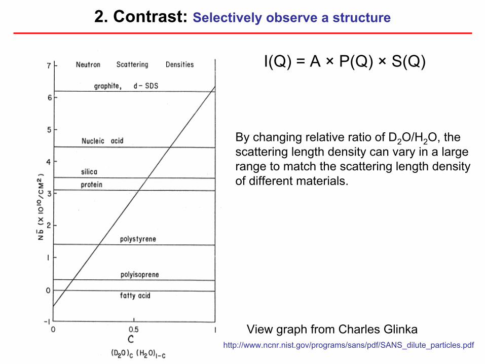
2. Contrast: Selectively observe a structure
View graph from Charles Glinkahttp://www.ncnr.nist.gov/programs/sans/pdf/SANS_dilute_particles.pdf
By changing relative ratio of D2
O/H2
O, thescattering length density can vary in a largerange to match the scattering length densityof different materials.
I(Q) = A ×
P(Q) ×
S(Q)
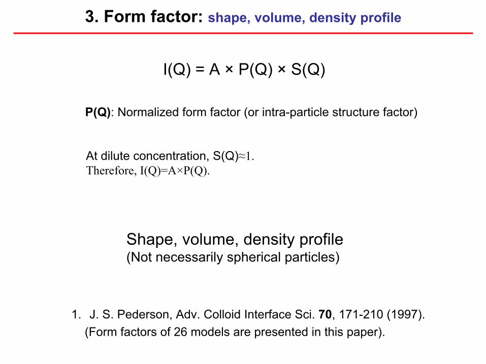
P(Q): Normalized form factor (or intra-particle structure factor)
At dilute concentration, S(Q)≈1.Therefore, I(Q)=A×P(Q).
1.
J. S. Pederson, Adv. Colloid Interface Sci. 70, 171-210 (1997).(Form factors of 26 models are presented in this paper).
Shape, volume, density profile(Not necessarily spherical particles)
3. Form factor: shape, volume, density profile
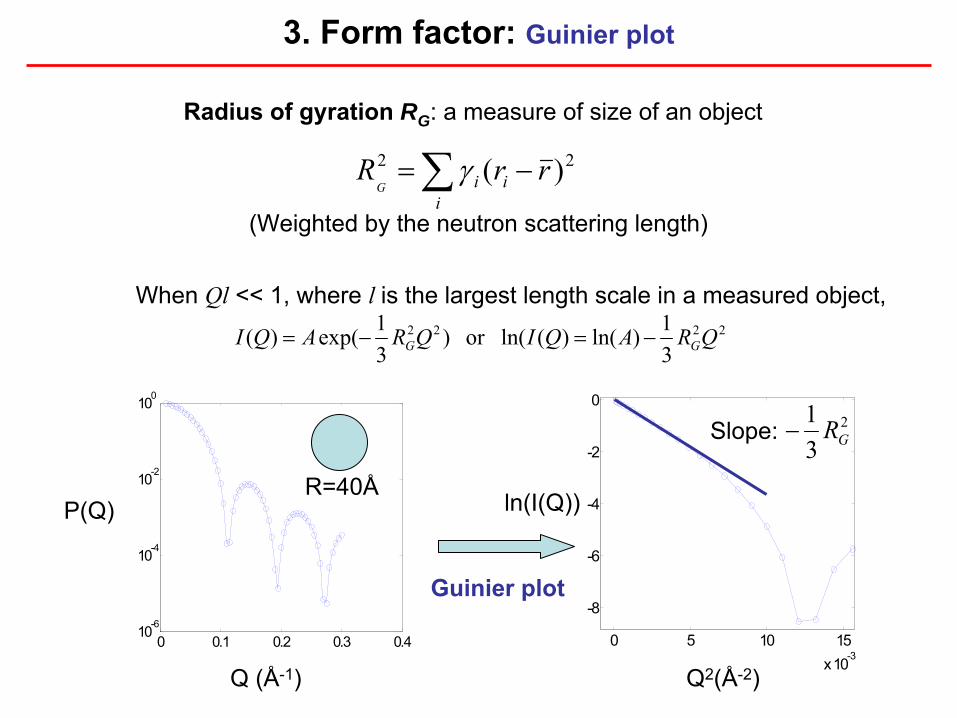
3. Form factor: Guinier
plot
Radius of gyration RG : a measure of size of an object
∑ −=i
ii rrRG
22 )(γ
(Weighted by the neutron scattering length)
2222
31)ln()(ln(or )
31exp()( QRAQIQRAQI GG −=−=
When Ql
<< 1, where l is the largest length scale in a measured object,
0 5 10 15x 10-3
-8
-6
-4
-2
0
ln(I(Q))
Q2(Å-2)
Slope: 2
31
GR−
Guinier
plot
0 0.1 0.2 0.3 0.410-6
10-4
10-2
100
P(Q)
Q (Å-1)
R=40Å
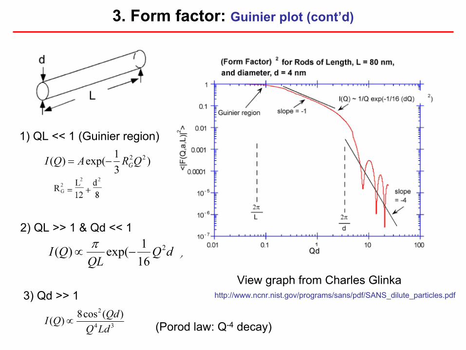
3. Form factor: Guinier
plot (cont’d)
2) QL >> 1 & Qd
<< 1
)161exp()( 22dQ
QLQI −∝
π
1) QL << 1 (Guinier
region)
)31exp()( 22QRAQI G−=
3) Qd
>> 1
34
2 )(cos8)(LdQ
QdQI ∝ (Porod
law: Q-4
decay)
View graph from Charles Glinkahttp://www.ncnr.nist.gov/programs/sans/pdf/SANS_dilute_particles.pdf
I(Q) = A ×
P(Q) ×
S(Q)
1.
A: Contrast terms2.
P(Q): Form factor (or intra-particle structure factor)3.
S(Q): Inter-particle structure factor
4. Structure factor S(Q): inter-particle potential
3
,
)1)((1
11
1)(
drergn
eeN
eeN
QS
riQ
kj
riQriQ
kj
riQriQ
kj
kj
⋅
≠
⋅⋅−
⋅⋅−
∫
∑
∑
−+=
+=
=
n: number densityg(r): pair distribution function
Zp
+ Zp
+-
-+
-
-
-
-
-
-
--
+
+ +
++
+
++
+
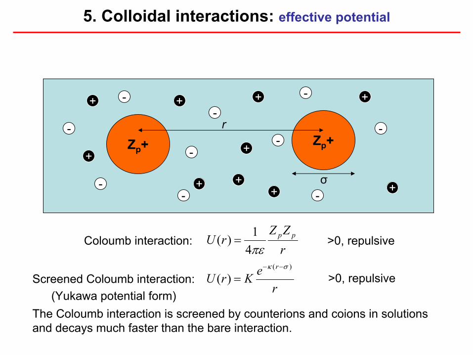
Coloumb
interaction:rZZ
rU pp
πε41)( = >0, repulsive
reKrU
r )(
)(σκ −−
=Screened Coloumb
interaction: >0, repulsive
The Coloumb
interaction is screened by counterions
and coions
in solutionsand decays much faster than the bare interaction.
(Yukawa potential form)
r
σ
5. Colloidal interactions: effective potential
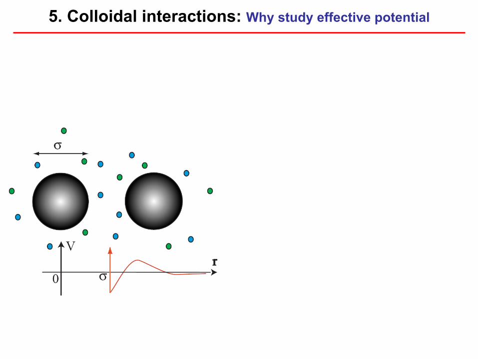
5. Colloidal interactions: Why study effective potential
Single Particle Information:Charge, Surface Properties, …
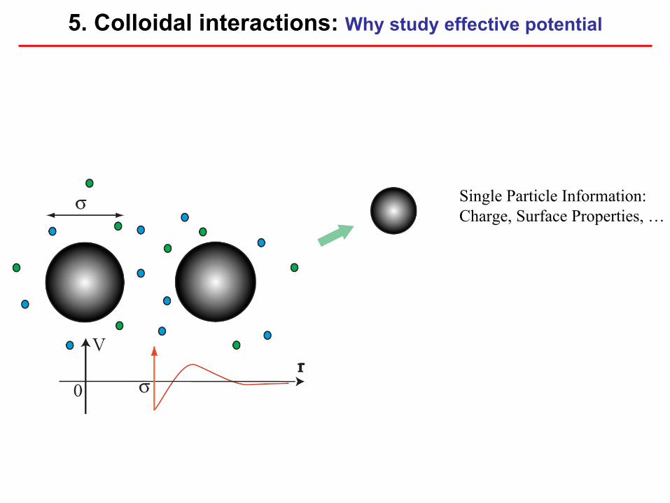
5. Colloidal interactions: Why study effective potential
Single Particle Information:Charge, Surface Properties, …
Collective Behaviors:Diffusion, Clusterization, …
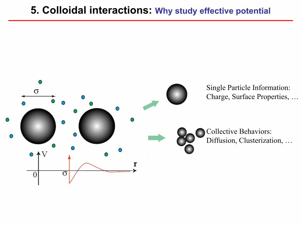
5. Colloidal interactions: Why study effective potential

Single Particle Information:Charge, Surface Properties, …
Collective Behaviors:Diffusion, Clusterization, …
Phase Behaviors:Liquid, Crystal, Glass, …
5. Colloidal interactions: Why study effective potential
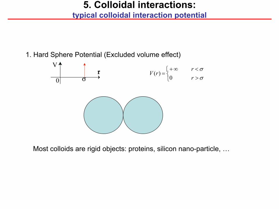
⎩⎨⎧
><∞+
=σσ
r r
rV 0
)(
1. Hard Sphere Potential (Excluded volume effect)
5. Colloidal interactions: typical colloidal interaction potential
Most colloids are rigid objects: proteins, silicon nano-particle, …
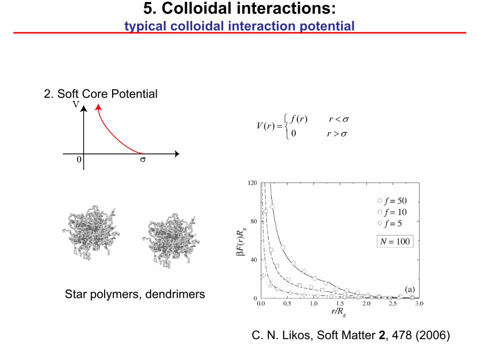
⎩⎨⎧
><
=σσ
r rrf
rV 0
)()(
2. Soft Core Potential
5. Colloidal interactions: typical colloidal interaction potential
C. N. Likos, Soft Matter 2, 478 (2006)
Star polymers, dendrimers
⎪⎪⎩
⎪⎪⎨
⎧
><<
<
⎥⎦
⎤⎢⎣
⎡⎟⎠⎞
⎜⎝⎛
−−
∞
=ar
arr
aarV σ
σ
στβ
012
1ln)(
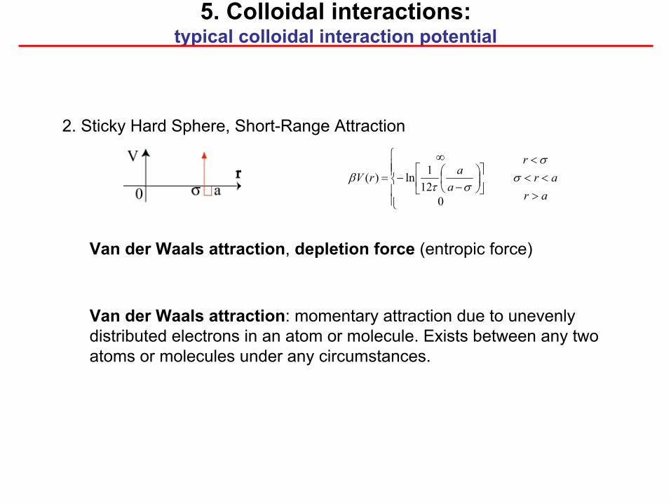
2. Sticky Hard Sphere, Short-Range Attraction
5. Colloidal interactions: typical colloidal interaction potential
Van der
Waals attraction, depletion force
(entropic force)
Van der
Waals attraction: momentary attraction due to unevenly distributed electrons in an atom or molecule. Exists between any
two atoms or molecules under any circumstances.
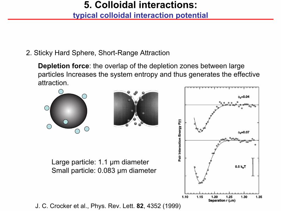
2. Sticky Hard Sphere, Short-Range Attraction
5. Colloidal interactions: typical colloidal interaction potential
Depletion force: the overlap of the depletion zones between large particles Increases the system entropy and thus generates the effective attraction.
Large particle: 1.1 μm diameterSmall particle: 0.083 μm diameter
J. C. Crocker et al., Phys. Rev. Lett. 82, 4352 (1999)
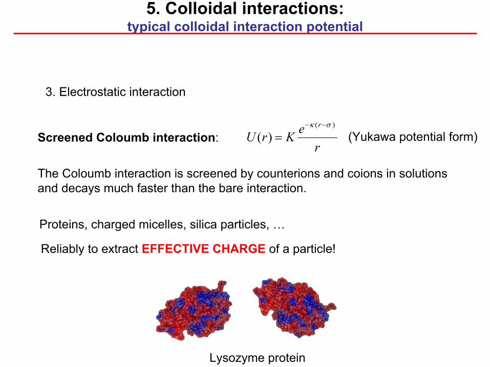
3. Electrostatic interaction
5. Colloidal interactions: typical colloidal interaction potential
reKrU
r )(
)(σκ −−
=Screened Coloumb
interaction:
The Coloumb
interaction is screened by counterions
and coions
in solutionsand decays much faster than the bare interaction.
(Yukawa potential form)
Proteins, charged micelles, silica particles, …
Lysozyme
protein
Reliably to extract EFFECTIVE CHARGE
of a particle!
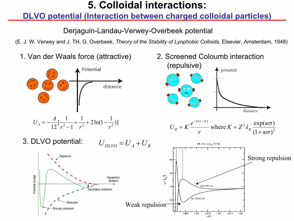
)]11ln(211
1[12 222 rrrAU A −++
−−=
1. Van der
Waals force (attractive)
22
)(
)1()exp( where
κσκσλ
σκ
+==
−−
B
r
R ZKr
eKU
2. Screened Coloumb
interaction(repulsive)
3. DLVO potential:RADLVO UUU +=
Strong repulsion
Weak repulsion
5. Colloidal interactions: DLVO potential (Interaction between charged colloidal particles)
Derjaguin-Landau-Verwey-Overbeek potential(E. J. W. Verwey
and J. TH. G. Overbeek, Theory of the Stability of Lyophobic
Colloids, Elsevier, Amsterdam, 1948)
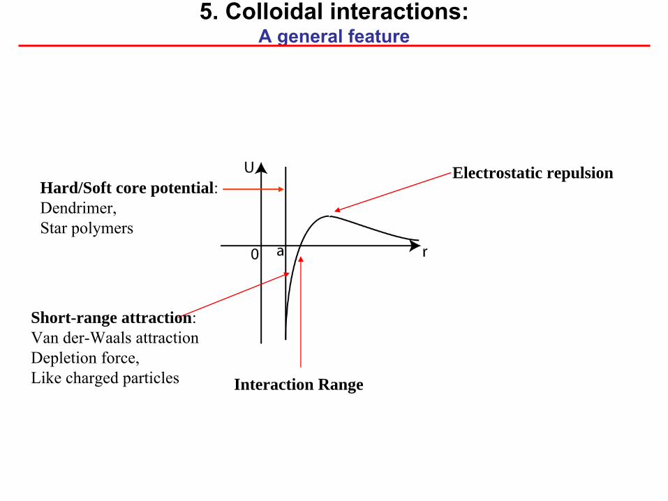
Short-range attraction:Van der-Waals
attractionDepletion force,Like charged particles Interaction Range
Electrostatic repulsionHard/Soft core potential:Dendrimer,Star polymers
5. Colloidal interactions: A general feature
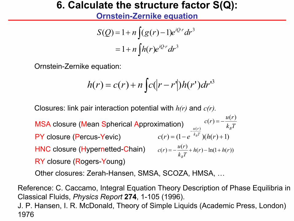
6. Calculate the structure factor S(Q): Ornstein-Zernike equation
3
3
)(1
)1)((1 )(
drerhn
drergnQSriQ
riQ
⋅
⋅
∫∫
+=
−+=
∫ −+= 3')'()'()()( drrhrrcnrcrh
Ornstein-Zernike equation:
Closures: link pair interaction potential with h(r)
and c(r).
MSA
closure (Mean Spherical Approximation)
RY
closure (Rogers-Young)
HNC
closure (Hypernetted-Chain) ))(1ln()()()( rhrhTkrurc
B
+−+−=
Tkrurc
B
)()( −=
PY
closure (Percus-Yevic) )1)()(1()()(
+−=−
rherc Tkru
B
Other closures: Zerah-Hansen, SMSA, SCOZA, HMSA, …
Reference: C. Caccamo, Integral Equation Theory Description of Phase Equilibria
in Classical Fluids, Physics Report
274, 1-105 (1996).J. P. Hansen, I. R. McDonald, Theory of Simple Liquids (Academic
Press, London) 1976
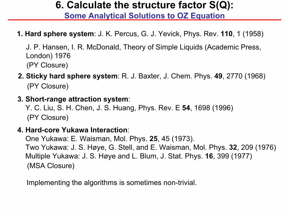
6. Calculate the structure factor S(Q): Some Analytical Solutions to OZ Equation
Implementing the algorithms is sometimes non-trivial.
1.
Hard sphere system: J. K. Percus, G. J. Yevick, Phys. Rev. 110, 1 (1958)
J. P. Hansen, I. R. McDonald, Theory of Simple Liquids (Academic
Press, London) 1976(PY Closure)
2.
Sticky hard sphere system: R. J. Baxter, J. Chem. Phys. 49, 2770 (1968)(PY Closure)
3.
Short-range attraction system: Y. C. Liu, S. H. Chen, J. S. Huang, Phys. Rev. E 54, 1698 (1996)(PY Closure)
4.
Hard-core Yukawa Interaction: One Yukawa: E. Waisman, Mol. Phys. 25, 45 (1973).Two Yukawa: J. S. Høye, G. Stell, and E. Waisman, Mol. Phys. 32, 209 (1976)Multiple Yukawa: J. S. Høye
and L. Blum, J. Stat. Phys. 16, 399 (1977)(MSA Closure)
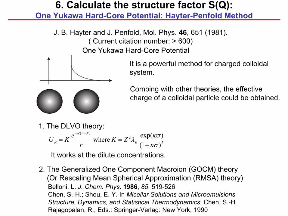
6. Calculate the structure factor S(Q): One Yukawa Hard-Core Potential: Hayter-Penfold
Method
J. B. Hayter
and J. Penfold, Mol. Phys. 46, 651 (1981).( Current citation number: > 600)
It is a powerful method for charged colloidal system.
Combing with other theories, the effectivecharge of a colloidal particle could be obtained.
1. The DLVO theory:
22
)(
)1()exp( where
κσκσλ
σκ
+==
−−
B
r
R ZKr
eKU
It works at the dilute concentrations.
2. The Generalized One Component Macroion
(GOCM) theory(Or Rescaling Mean Spherical Approximation (RMSA) theory)Belloni, L. J. Chem. Phys. 1986, 85, 519-526Chen, S.-H.; Sheu, E. Y. In Micellar
Solutions and Microemulsions-Structure, Dynamics, and Statistical Thermodynamics; Chen, S.-H.,Rajagopalan, R., Eds.: Springer-Verlag: New York, 1990
One Yukawa
Hard-Core Potential
M.Broccio, D.Costa, Y.Liu, S.H. Chen, JCP
124, 084501 (2006)
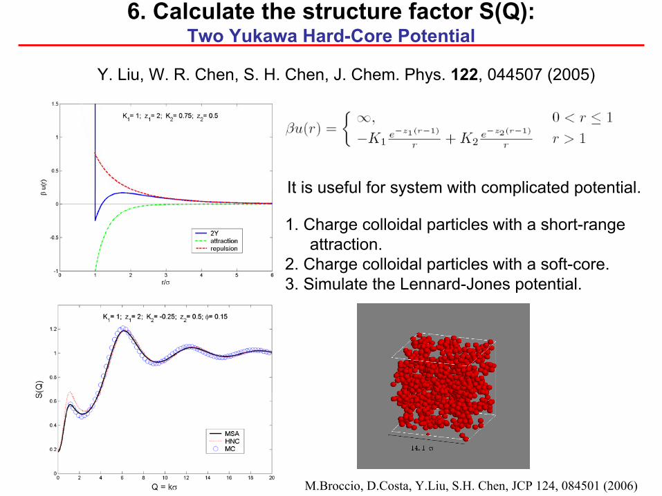
6. Calculate the structure factor S(Q): Two Yukawa Hard-Core Potential
Y. Liu, W. R. Chen, S. H. Chen, J. Chem. Phys. 122, 044507 (2005)
It is useful for system with complicated potential.
1. Charge colloidal particles with a short-rangeattraction.
2. Charge colloidal particles with a soft-core.3. Simulate the Lennard-Jones potential.
Advantage of a numerical methods:• Trivial to extend the method to more complicated potential• Easy to extend to all kinds of different closures (HNC, RY, Zerah-Hansen, SCOZA,…)• The validity of new methods could be easily verified by computer simulations• Relatively easy to implement the thermodynamic consistency
The development of powerful computerNumerical Solutions
6. Calculate the structure factor S(Q): Numerical Solutions to OZ Equation
C. Caccamo, Integral Equation Theory Description of Phase Equilibria
in Classical Fluids, Physics Report
274, 1-105 (1996). And references therein.
Application of numerical solution to analyze the scattering results of colloidal systemsbecomes more and more important.
DLVO (HNC), One Yukawa (HNC) (protein solutions)
Two Yukawa (HNC) (protein solutions, micellar
systems)
Many Examples ! Such as
M.Broccio, D.Costa, Y.Liu, S.H. Chen, JCP
124, 084501 (2006)
A. Tardieu, S. Finet, and F. Bonnete´, J. Cryst. Growth 232, 1 (2001).
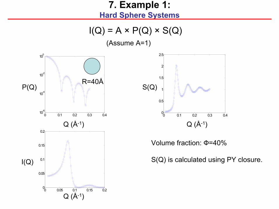
7. Example 1: Hard Sphere Systems
0 0.1 0.2 0.3 0.410-6
10-4
10-2
100
P(Q)
Q (Å-1)
R=40Å
I(Q) = A ×
P(Q) ×
S(Q)(Assume A=1)
0 0.1 0.2 0.3 0.40
0.5
1
1.5
2
2.5
S(Q)
Q (Å-1)
0 0.05 0.1 0.15 0.20
0.05
0.1
0.15
0.2
I(Q)
Q (Å-1)
Volume fraction: Ф=40%
S(Q) is calculated using PY closure.
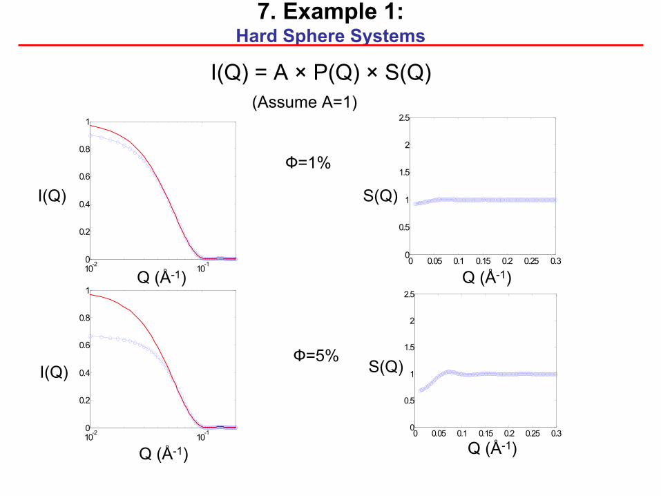
7. Example 1: Hard Sphere Systems
I(Q) = A ×
P(Q) ×
S(Q)(Assume A=1)
Ф=1%
10-2 10-10
0.2
0.4
0.6
0.8
1
0 0.05 0.1 0.15 0.2 0.25 0.30
0.5
1
1.5
2
2.5
10-2 10-10
0.2
0.4
0.6
0.8
1
0 0.05 0.1 0.15 0.2 0.25 0.30
0.5
1
1.5
2
2.5
Ф=5%I(Q)
Q (Å-1)
I(Q)
Q (Å-1)
S(Q)
Q (Å-1)
S(Q)
Q (Å-1)
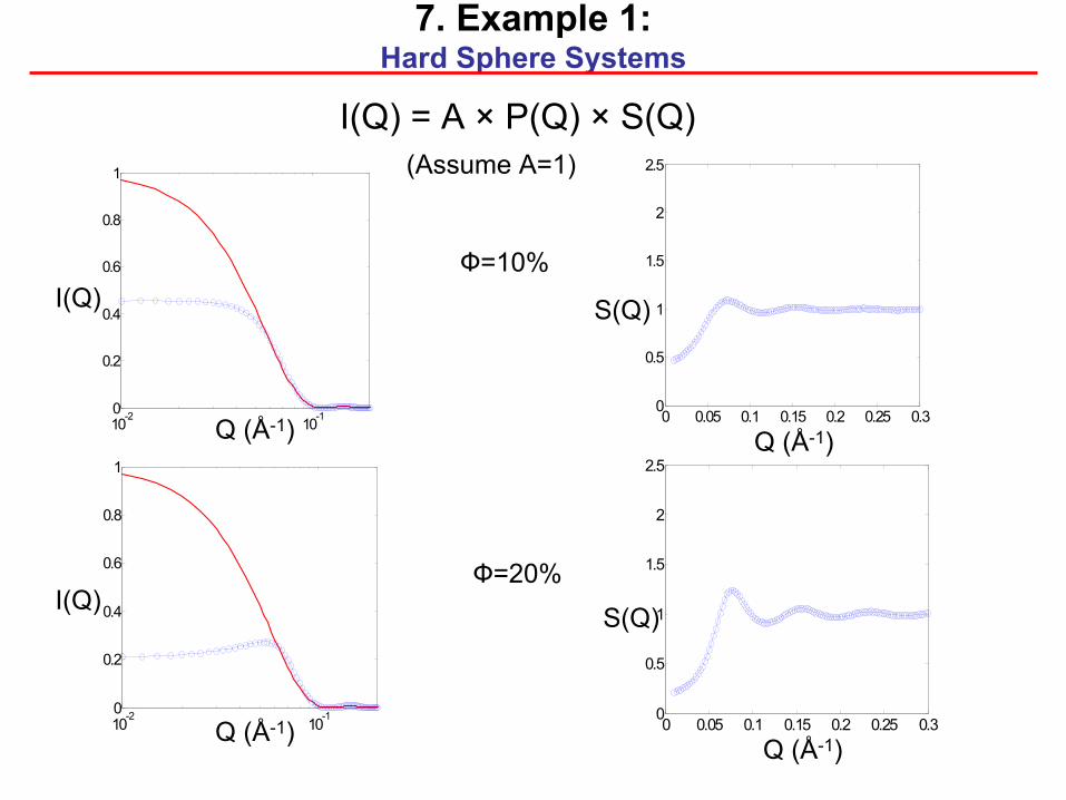
7. Example 1: Hard Sphere Systems
I(Q) = A ×
P(Q) ×
S(Q)(Assume A=1)
Ф=10%
Ф=20%
10-2 10-10
0.2
0.4
0.6
0.8
1
0 0.05 0.1 0.15 0.2 0.25 0.30
0.5
1
1.5
2
2.5
10-2 10-10
0.2
0.4
0.6
0.8
1
0 0.05 0.1 0.15 0.2 0.25 0.30
0.5
1
1.5
2
2.5
I(Q)
Q (Å-1)
I(Q)
Q (Å-1)
S(Q)
Q (Å-1)
S(Q)
Q (Å-1)
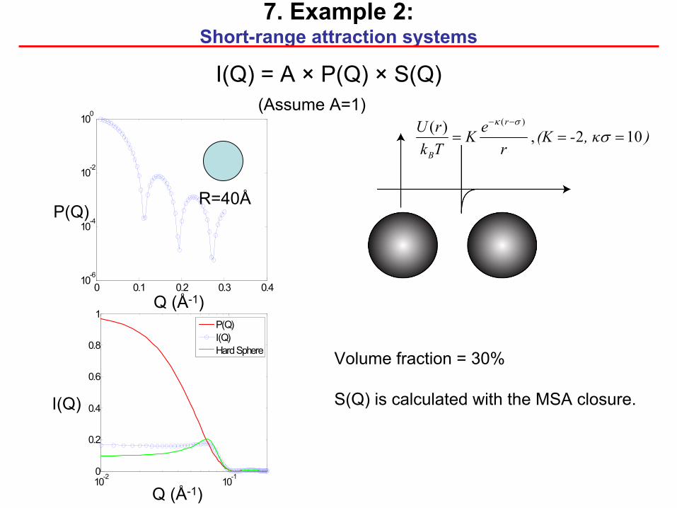
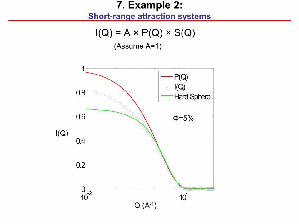
7. Example 2: Short-range attraction systems
I(Q) = A ×
P(Q) ×
S(Q)(Assume A=1)
0 0.1 0.2 0.3 0.410-6
10-4
10-2
100
P(Q)
Q (Å-1)
R=40Å
), κ-(Kr
eKTkrU r
B
102 , )( )(
===−−
σσκ
Volume fraction = 30%
S(Q) is calculated with the MSA closure.
10-2 10-10
0.2
0.4
0.6
0.8
1
P(Q)I(Q)Hard Sphere
I(Q)
Q (Å-1)
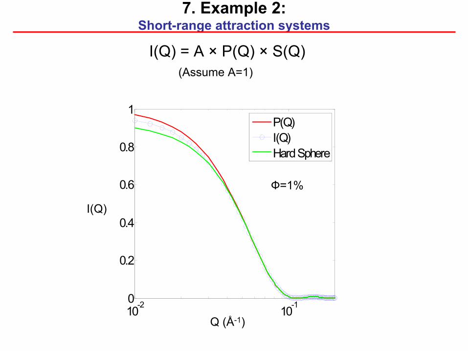
7. Example 2: Short-range attraction systems
I(Q) = A ×
P(Q) ×
S(Q)(Assume A=1)
10-2 10-10
0.2
0.4
0.6
0.8
1
P(Q)I(Q)Hard Sphere
Ф=1%
I(Q)
Q (Å-1)
10-2 10-10
0.2
0.4
0.6
0.8
1
P(Q)I(Q)Hard Sphere
7. Example 2: Short-range attraction systems
I(Q) = A ×
P(Q) ×
S(Q)(Assume A=1)
Ф=5%
I(Q)
Q (Å-1)
10-2 10-10
0.2
0.4
0.6
0.8
1
P(Q)I(Q)Hard Sphere
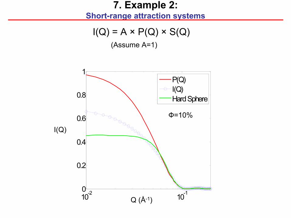
7. Example 2: Short-range attraction systems
I(Q) = A ×
P(Q) ×
S(Q)(Assume A=1)
Ф=10%
I(Q)
Q (Å-1)
10-2 10-10
0.2
0.4
0.6
0.8
1
P(Q)I(Q)Hard Sphere
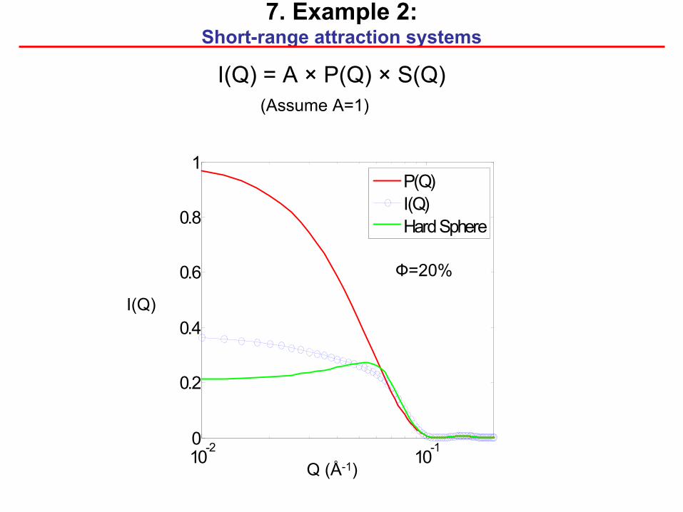
7. Example 2: Short-range attraction systems
I(Q) = A ×
P(Q) ×
S(Q)(Assume A=1)
Ф=20%
I(Q)
Q (Å-1)
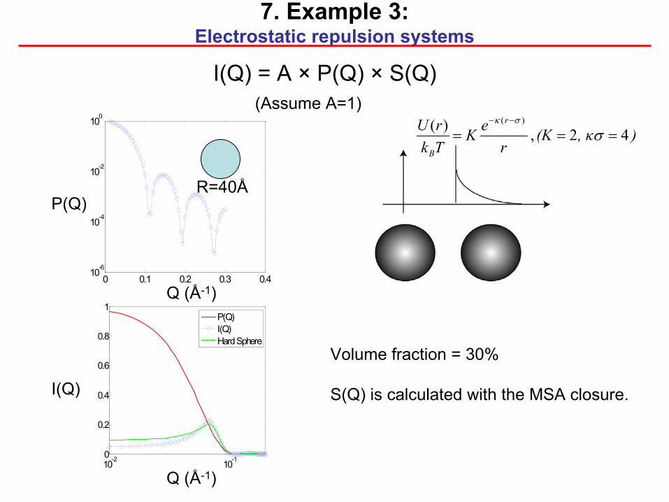
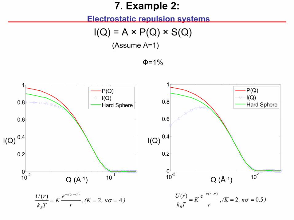
7. Example 3: Electrostatic repulsion systems
I(Q) = A ×
P(Q) ×
S(Q)(Assume A=1)
0 0.1 0.2 0.3 0.410-6
10-4
10-2
100
), κ(Kr
eKTkrU r
B
42 , )( )(
===−−
σσκ
Volume fraction = 30%
S(Q) is calculated with the MSA closure.
10-2 10-10
0.2
0.4
0.6
0.8
1
P(Q)I(Q)Hard Sphere
R=40Å
I(Q)
Q (Å-1)
P(Q)
Q (Å-1)
10-2 10-10
0.2
0.4
0.6
0.8
1
P(Q)I(Q)Hard Sphere
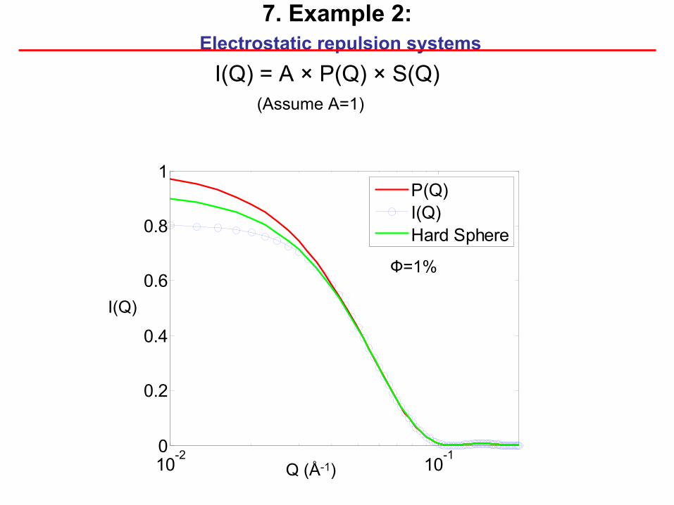
7. Example 2: Electrostatic repulsion systems
I(Q) = A ×
P(Q) ×
S(Q)(Assume A=1)
Ф=1%
I(Q)
Q (Å-1)
10-2 10-10
0.2
0.4
0.6
0.8
1
P(Q)I(Q)Hard Sphere
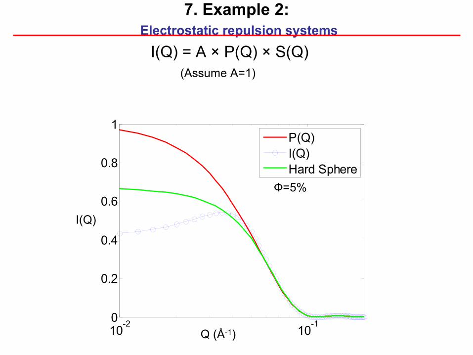
7. Example 2: Electrostatic repulsion systems
I(Q) = A ×
P(Q) ×
S(Q)(Assume A=1)
Ф=5%
I(Q)
Q (Å-1)
10-2 10-10
0.2
0.4
0.6
0.8
1
P(Q)I(Q)Hard Sphere
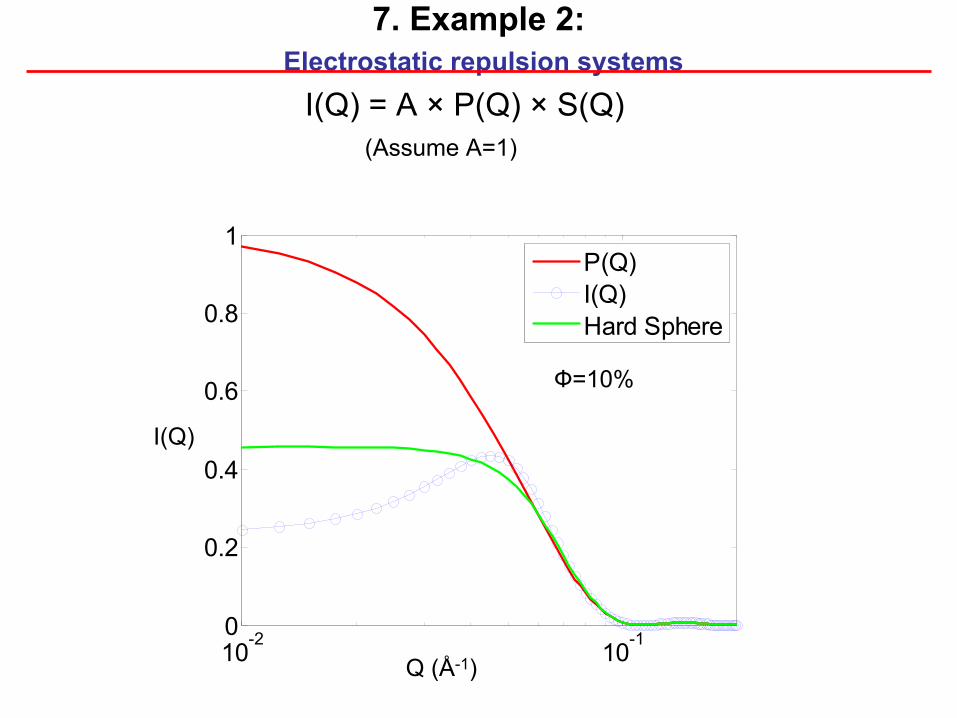
7. Example 2: Electrostatic repulsion systems
I(Q) = A ×
P(Q) ×
S(Q)(Assume A=1)
Ф=10%
I(Q)
Q (Å-1)
10-2 10-10
0.2
0.4
0.6
0.8
1
P(Q)I(Q)Hard Sphere
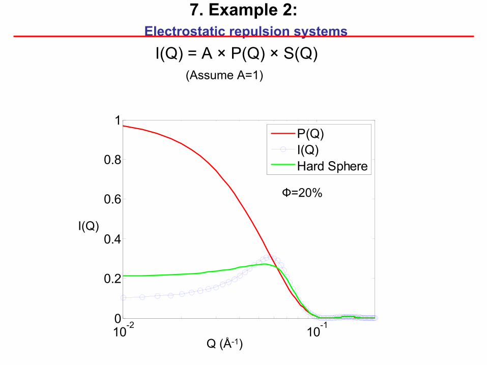
7. Example 2: Electrostatic repulsion systems
I(Q) = A ×
P(Q) ×
S(Q)(Assume A=1)
Ф=20%
I(Q)
Q (Å-1)
10-2 10-10
0.2
0.4
0.6
0.8
1
P(Q)I(Q)Hard Sphere
10-2 10-10
0.2
0.4
0.6
0.8
1
P(Q)I(Q)Hard Sphere
7. Example 2: Electrostatic repulsion systems
I(Q) = A ×
P(Q) ×
S(Q)(Assume A=1)
Ф=1%
), κ(Kr
eKTkrU r
B
42 , )( )(
===−−
σσκ
), κ(Kr
eKTkrU r
B
5.02 , )( )(
===−−
σσκ
I(Q)
Q (Å-1)
I(Q)
Q (Å-1)

7. Example 2: Electrostatic repulsion systems
I(Q) = A ×
P(Q) ×
S(Q)(Assume A=1)
Ф=0.5%
), κ(Kr
eKTkrU r
B
5.02 , )( )(
===−−
σσκ
10-2 10-10
0.2
0.4
0.6
0.8
1
P(Q)I(Q)Hard Sphere
10-2 10-10
0.2
0.4
0.6
0.8
1
P(Q)I(Q)Hard Sphere
Ф=0.1%
I(Q)
Q (Å-1)
I(Q)
Q (Å-1)
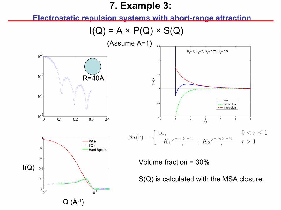
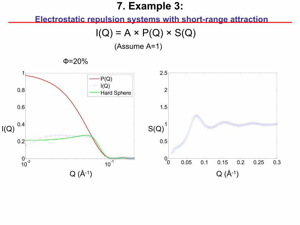
7. Example 3: Electrostatic repulsion systems with short-range attraction
I(Q) = A ×
P(Q) ×
S(Q)(Assume A=1)
0 0.1 0.2 0.3 0.410-6
10-4
10-2
100
R=40Å
10-2 10-10
0.2
0.4
0.6
0.8
1
P(Q)I(Q)Hard Sphere
Volume fraction = 30%
S(Q) is calculated with the MSA closure.
I(Q)
Q (Å-1)
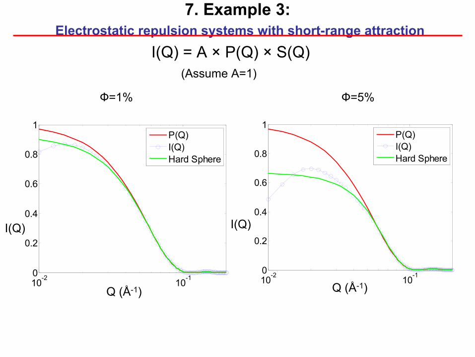
7. Example 3: Electrostatic repulsion systems with short-range attraction
I(Q) = A ×
P(Q) ×
S(Q)(Assume A=1)
10-2 10-10
0.2
0.4
0.6
0.8
1
P(Q)I(Q)Hard Sphere
Ф=1%
10-2 10-10
0.2
0.4
0.6
0.8
1
P(Q)I(Q)Hard Sphere
Ф=5%
I(Q)
Q (Å-1)
I(Q)
Q (Å-1)
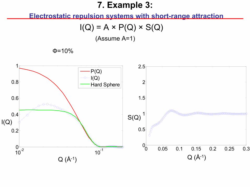
7. Example 3: Electrostatic repulsion systems with short-range attraction
I(Q) = A ×
P(Q) ×
S(Q)(Assume A=1)
Ф=10%
10-2 10-10
0.2
0.4
0.6
0.8
1
P(Q)I(Q)Hard Sphere
0 0.05 0.1 0.15 0.2 0.25 0.30
0.5
1
1.5
2
2.5
I(Q)
Q (Å-1)
S(Q)
Q (Å-1)
7. Example 3: Electrostatic repulsion systems with short-range attraction
I(Q) = A ×
P(Q) ×
S(Q)(Assume A=1)
Ф=20%
10-2 10-10
0.2
0.4
0.6
0.8
1
P(Q)I(Q)Hard Sphere
0 0.05 0.1 0.15 0.2 0.25 0.30
0.5
1
1.5
2
2.5
I(Q)
Q (Å-1)
S(Q)
Q (Å-1)
10-2 10-10
0.2
0.4
0.6
0.8
1
P(Q)I(Q)Hard Sphere
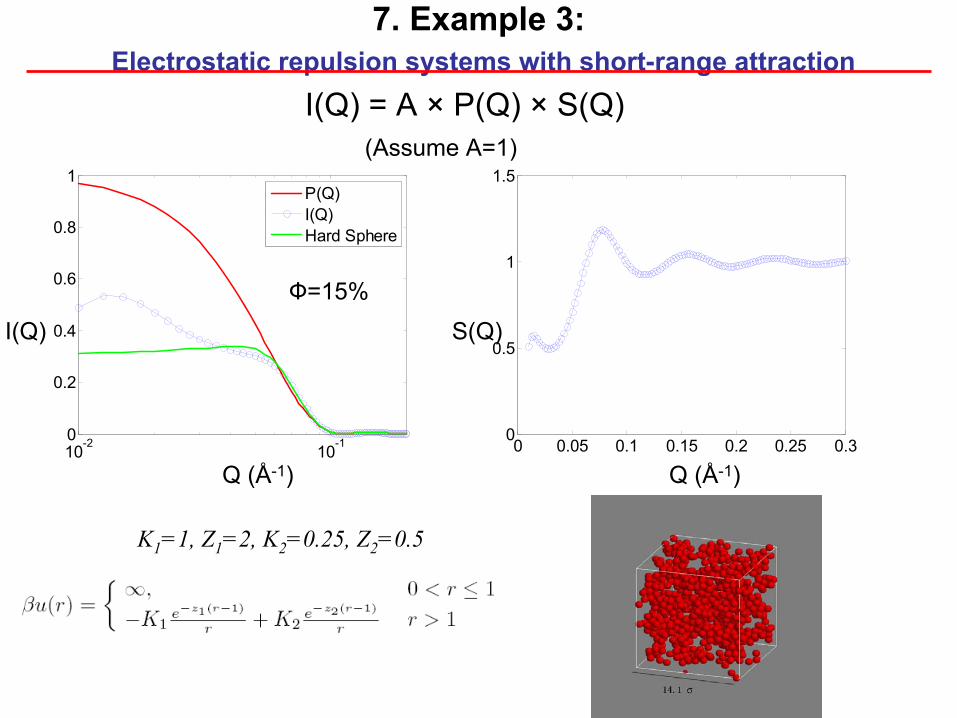
7. Example 3: Electrostatic repulsion systems with short-range attraction
I(Q) = A ×
P(Q) ×
S(Q)(Assume A=1)
Ф=15%
0 0.05 0.1 0.15 0.2 0.25 0.30
0.5
1
1.5
K1
=1, Z1
=2, K2
=0.25, Z2
=0.5
I(Q)
Q (Å-1)
S(Q)
Q (Å-1)
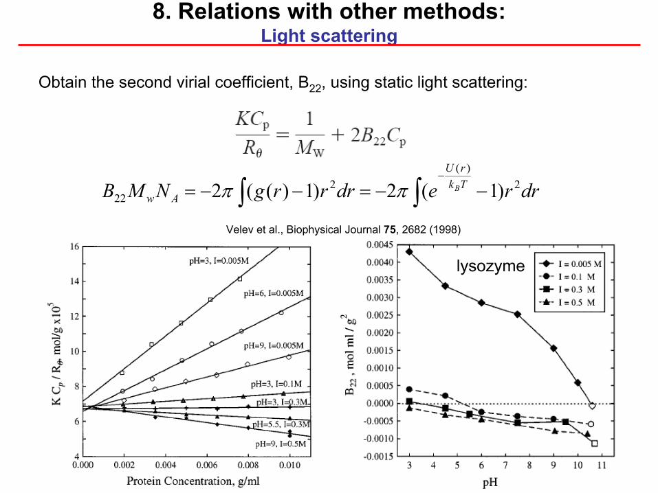
8. Relations with other methods: Light scattering
Obtain the second virial
coefficient, B22
, using static light scattering:
∫∫ −−=−−=−
drredrrrgNMB TkrU
AwB 2
)(2
22 )1(2)1)((2 ππ
lysozyme
Velev
et al., Biophysical Journal 75, 2682 (1998)
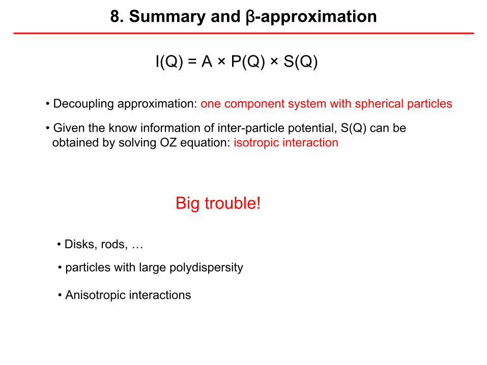
8. Summary and β-approximation
I(Q) = A ×
P(Q) ×
S(Q)
• Decoupling approximation: one component system with spherical particles
• Given the know information of inter-particle potential, S(Q) can be obtained by solving OZ equation: isotropic interaction
Big trouble!
• Disks, rods, …
• particles with large polydispersity
• Anisotropic interactions
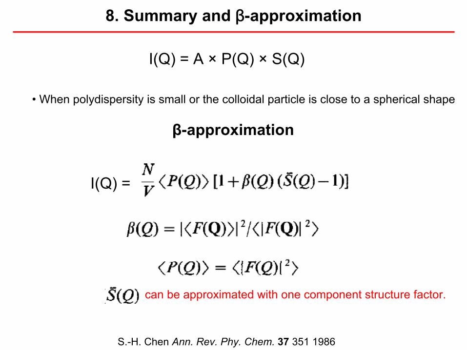
8. Summary and β-approximation
I(Q) = A ×
P(Q) ×
S(Q)
• When polydispersity
is small or the colloidal particle is close to a spherical shape
S.-H. Chen Ann. Rev. Phy. Chem.
37
351 1986
I(Q) =
β-approximation
can be approximated with one component structure factor.
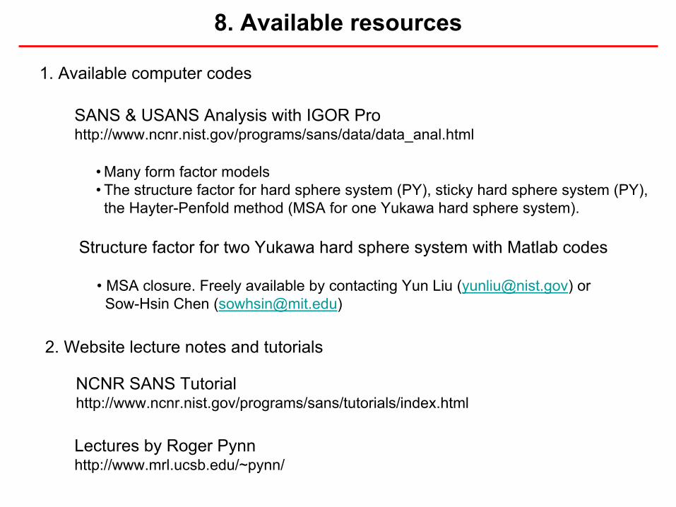
8. Available resources
1. Available computer codes
SANS & USANS Analysis with IGOR Prohttp://www.ncnr.nist.gov/programs/sans/data/data_anal.html
•
Many form factor models •
The structure factor for hard sphere system (PY), sticky hard sphere system (PY), the Hayter-Penfold
method (MSA for one Yukawa hard sphere system).
Structure factor for two Yukawa hard sphere system with Matlab
codes
• MSA closure. Freely available by contacting Yun
Liu ([email protected]) orSow-Hsin
Chen ([email protected])
2. Website lecture notes and tutorials
NCNR SANS Tutorialhttp://www.ncnr.nist.gov/programs/sans/tutorials/index.html
Lectures by Roger Pynnhttp://www.mrl.ucsb.edu/~pynn/