Combined Charge Spin and Momentum Densities Refinement : Application to Magnetic Molecular Materials

Claude Lecomtea, Maxime Deutscha, Mohamed Souhassoua, Nicolas Claisera, Sebastien Pilleta,

Pierre Beckerb, Jean-Michel Gilletb, Béatrice Gillonc and Dominique Luneaud

a Laboratoire de Cristallographie, Résonance Magnétique et Modélisations (UMR CNRS 7036), BP 70239,

54506 Vandoeuvre-lès-Nancy France.

b Laboratoire. S.P.M.S., UMR CNRS 8580, École Centrale Paris, Grande Voie des Vignes, 92295 Chatenay-

Malabry France.

c Laboratoire Léon Brillouin (CEA-CNRS, UMR 12), Centre d'Etudes de Saclay, 91191 Gif-sur-Yvette France.

d Laboratoire des Multimatériaux et Interfaces (UMR 5615), Université Claude Bernard Lyon-1, 69622

Villeurbanne Cedex (France)

Introduction Interaction between crystals and X-ray/polarized neutrons, is due to all/unpaired electrons and allow describing and modelling the charge and spin density in position space (Coppens, 1997, Brown et al, 1980) (X-ray / polarized neutron diffraction) and in momentum space (Compton scattering / magnetic Compton scattering) (Cooper et al, 2004). Nowadays, models are mostly derived from one single experiment: X-ray diffraction and charge density modelling, polarized neutron diffraction and spin density modelling... and few attempts have been made to combine several experiments in order to have a more general and thorough electron density modelling. P. Coppens et al (1981) were among the first to propose a joint X-ray/neutron refinement in order to limit the effects of correlation between structural and charge density parameters. This X+N multipolar refinement (Hansen & Coppens 1978) was applied on oxalic acid dehydrate and it was found that the X+N model deformation density shows higher peaks in the lone pair regions. The weighting schemes have been discussed but are not of primary importance in that case because the number of neutron and X-ray diffraction data was similar; it was also shown that the dependence of the x,y,z,Uij structural parameters was in line with their X/N form factors. Schwarzenbach and co-workers (Lewis et al, 1982) have refined the charge density in α Al2O3 with respect to very accurate ultra high resolution data (1.5 Å-1) with AgKα radiation under the constraints of electric field gradient tensors at both Al and O atomic sites, using Hirshfeld deformation functions (Hirshfeld, 1977) and showed that this joint refinement mainly affects the quadrupolar deformation terms as expected. However the very strong anisotropic extinction did not allow drawing more conclusions about the quality of the density. More recently, several papers

report on the possibility to recover the diagonal part of the one particle reduced density matrix (1-RDM for more details see part 5):

( ) 4 41 1 1 2 1 2 2

*N N N; ' N ( , , , ) ( ' , , , )d d= ∫x x x x x x x x x x… … …Γ ψ ψ (1)

from X-ray refinements by minimizing the resulting energy (Jayatilaka & Grimwood, 2001, Grimwood & Jayatilaka, 2001, Bytheway et al., 2002b, Bytheway et al., 2002a, Grimwood et al., 2003) or imposing mathematical constraints like idempotency (Tanaka, 1988, Howard et al, 1994, Massa et al, 1985). All this research has been performed to give a more reliable model of the paired electron density in position space than from X-ray data refinement solely. In the case of magnetic crystals, the description of the electronic structure in position space relies on two diffraction experiments: - X-rays for all electron density - polarized neutrons (PN) for unpaired electron density. Both may be modelled using the Hansen Coppens multipole model (in the polarized neutrons experiment there are no core contributions to the scattering):

maxl l

3 3core val v l lm lm

l 0 m 0

( r ) ( r ) P ( r ) ' R ( ' r ) P y ( , )ρ ρ κ ρ κ κ κ θ φ± ±= =

= + + ∑ ∑

(2)

where ylm are the real spherical harmonics which differ from the corresponding Ylmp by normalizing conditions, R(κ’r ) are Slater type functions, κ and κ’ are expansion contraction coefficients. The net charge of the atom or spin population were estimated from the Pv/Poo parameters obtained respectively from X-ray and PN diffraction data but never from a joint X-ray, PND refinement as proposed by Becker & Coppens (1985). One of the problems to perform such a joint least squares refinement is the unbalanced number of observations as discussed below. According to the Hohenberg-Kohn theorem, if such a joint diffraction approach may yield an exact experimental

density and by consequence, the diagonal part of ( )11 ';xxΓ , the non diagonal parts related to the

more delocalized electrons are out of reach. One of the possibilities is to study the electron density, paired or unpaired in momentum space: hence, due to the Heisenberg principle, the more delocalized electrons like conduction electrons in position space will have a compact representation in momentum space. Such a representation could be deduced from inelastic incoherent Compton scattering which gives the projection of the e- momentum on the scattering vector (see for example Hayashi et al, 2002). These projections are known as directional Compton profiles (for a general review on Compton scattering, see Cooper et al, 2004). Because it is mostly sensitive to very delocalized electrons, little work has been done on molecular solids. The major problem to deal with molecular compounds is that all contributions are superimposed and it is difficult to assign electrons to a particular pseudo atom or chemical site as shown below. Then, the one particule reduced density matrix can be seen as a unifying quantity and can be modelled by a joint refinement against X-ray and neutron scattering data. This paper is divided in five parts. In the first part, we will present the principles of charge density modelling.

The second part is devoted to spin density measurements. The third part will propose a strategy for a joint X-rays, neutron and polarized neutrons refinement The next part gives preliminary results applied to an end-to-end Azido Double Bridged CuII di nuclear complex (Cu2L2(N3)2) (L=1,1,1-trifluoro-7-(dimethylamino)-4-methyl-5-aza-3-hepten-2-onato). The last part will discuss how to go further in taking into account the non-magnetic and magnetic Compton scattering data. 1 Charge density measurement and modelling

In the kinematic approximation, the intensity of a Bragg reflection is proportional to the square of

the structure factor amplitude, ( )2

oF ; (for more details see, Blessing & Lecomte, 1991)

[ ] 223 **)/( oeoBragg FPLAVvrII λ≈ (3)

with Io the intensity of the incident X-rays beam supposed homogeneous and bathing the whole crystal, λ the wavelength, re the classical electron radius, L the Lorentz correction, P the polarization factor and A is the absorption factor. The measured intensity includes the Bragg reflection along with other contributions for which appropriate and accurate corrections are required:

[ ]1meas Bragg m Bragg m bkgm

I ( ) K I ( ) ( ) y( ) p I ( ) Iα= + + +∑H H H H H (4)

meas 1 m Bragg m bkgm

I ( ) KI ( ) p I ( ) I= + +∑H H H

The background (bkg) includes: Compton scattering, scattering by crystal mount, by air, fluorescence… Multiple scattering should also be corrected for: several reciprocal lattice points Hm may be in reflecting position simultaneously with H , α is the thermal diffuse contribution at the Bragg reflection and y the extinction coefficient:

yLPA

IKF

)1(

' 12

0 α+= (5)

To accurately model the crystal electron density in position space a very high resolution diffraction experiment at low temperature has to be performed so that the valence electron density (which diffuses at low resolution) is deconvoluted from thermal smearing effects (Debye Waller factor); the diffracted intensities are reduced in a set of dynamic structure factors amplitudes Fo(H) and their associated standard deviations. Fo(H) are the Fourier components of the experimental dynamic electron density :

( ) ( ) 2 3i .o maille

F e dπρ= ∫H rH r r

with ( ) ( ) ( )urr Pstat ⊗= ρρ = ∫ − uuur 3)()( dPstatρ .

In the harmonic approximation, for a given atom in the unit cell,

( )

112

3

1

2

j kjk ( u u )

P( ) eσ

π σ

−−=u (6)

Where σ is the determinant ( product of the three eigen values ) by convolution theorem, the dynamic structure factor is:

( ) 2

1

j

Nati .

dyn j jj

F f e T ( )π

== ∑

H rH H (7)

The static structure factor is therefore:

( ) ( ) 2

1

j

Nati .

Stat jj

F f eπ

==∑

H rH H (8)

where fj is the scattering (or form) factor of atom j, Fourier transform of the total atomic electron density:

2 3i .

Vf ( ) ( )e dπρ= ∫

H rH r r (9)

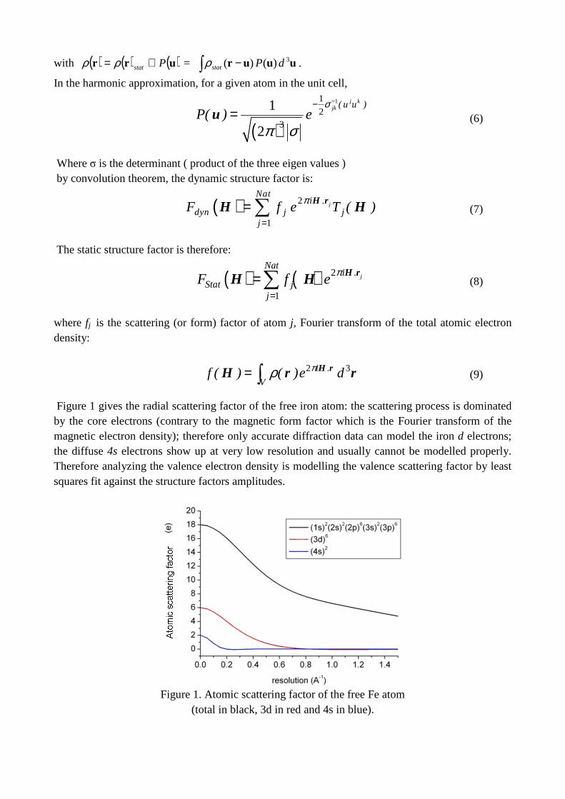
Figure 1 gives the radial scattering factor of the free iron atom: the scattering process is dominated by the core electrons (contrary to the magnetic form factor which is the Fourier transform of the magnetic electron density); therefore only accurate diffraction data can model the iron d electrons; the diffuse 4s electrons show up at very low resolution and usually cannot be modelled properly. Therefore analyzing the valence electron density is modelling the valence scattering factor by least squares fit against the structure factors amplitudes.

Figure 1. Atomic scattering factor of the free Fe atom

(total in black, 3d in red and 4s in blue).

This fit can be performed within the Hansen Coppens formalism (Hansen Coppens, 1978)

∑∑=

±±=

++=l

0mlmlm

l

llvalvcore yPrRPrr

max

),()'(')r()()(0

33 ϕθκκκρκρρ (10)

The corresponding scattering (or form ) factor for any ylm multipole density is

lnlm nl lmf ( ) i f ( H )y ( u,v )=H (11)

where u,v are the angular coordinates of vector H. The refined parameters are the expansion contraction coefficients κ,κ’ and the Pval and Plm populations

This allows computing static deformation maps

l max l

3 3stat val v val v l lm lm

l 0 m 0

( ) P ( r ) N ( r ) ' R ( ' r ) P y ( , )∆ρ κ ρ κ ρ κ κ θ φ± ±= =

= − + ∑ ∑r (12)

The Plm populations , l = 2 and 4, are related to the d orbitals populations through linear equations (Holladay et al, 1983) under the assumption that covalency is negligible; this can be applied to charge and spin density analysis .

2 Spin density measurements In PND experiments, a monochromatic polarized neutron beam with polarization vector P is

diffracted by a magnetically ordered single crystal. The diffracted intensities I+(ΚΚΚΚ) and I-(ΚΚΚΚ) of the

Bragg reflection with scattering vector K =2πH depend on the direction of polarization of the incident beam, parallel or antiparallel to the vertical applied magnetic field:

( ) ( ) 2

N MI ( ) F . ⊥± = ±K K P F K

(13)

where FN and FM refer to nuclear and magnetic structure factors. The magnetic structure factor

( )MF K is a vector, the direction of which is that of the magnetic moment µµµµ resulting from the

sum of the atomic moments µµµµι due to spin and orbit in the unit cell. Its magnitude is related to the normalized magnetization density m(r) by Fourier transform:

( ) ( ) i

cell

m e d= ∫Kr

MF K µ r r (14)

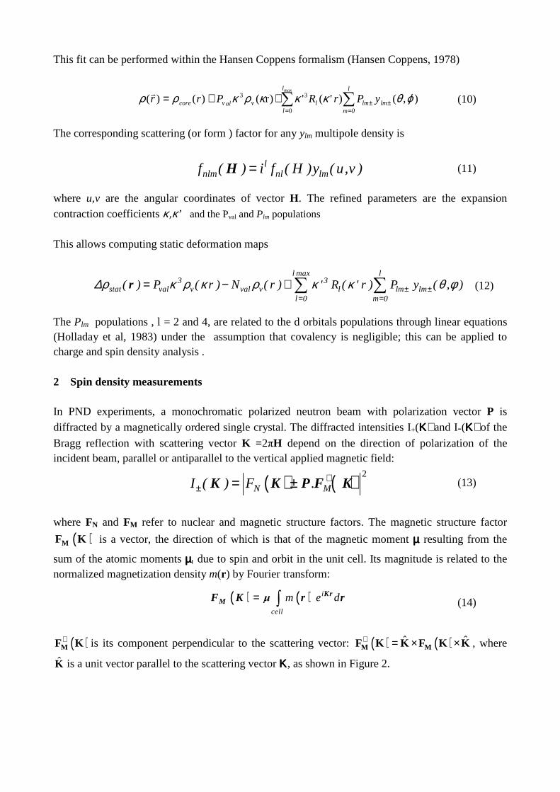
( )⊥MF K is its component perpendicular to the scattering vector: ( ) ( )ˆ ˆ⊥ = × ×M MF K K F K K , where

K is a unit vector parallel to the scattering vector ΚΚΚΚ, as shown in Figure 2.

Figure 2: Orientation of the induced magnetic structure factor for a magnetic field // z

If the atomic magnetic moments µµµµi are collinear with the applied magnetic field (this is the case for a paramagnetic compound without strong magnetic anisotropy), the magnetic structure factor

( )MF K is parallel to the vertical magnetic field and its component ( )⊥MF K is equal to FM(K)

sin2α, α being the angle between the vertical magnetization direction and the scattering vector. The experimental quantities measured by PND are the so-called flipping ratios R(ΚΚΚΚ):

( ) ( )( )

IR

I+

−=

KK

K (15)

In the case of a centric space group, the expression of the flipping ratio is:

( )2 2 2 2

N N M M2 2 2 2

N N M M

F 2Pq F F q FR

F 2Peq F F q F

+ +=− +

K (16)

where P is the polarisation rate, e is the flipping efficiency and q2 = (sinα)2.

The expression (16) is related to both FN and FM and therefore the determination of FM from the experimental flipping ratio requires the knowledge of FN. This is the reason why an unpolarized neutron diffraction experiment is generally performed before the PND data collection in order to determine precisely the nuclear structure at low temperature (closest as possible to the PND experimental conditions) i.e. the position and thermal parameters including those of the H atoms. Expression (16) leads to a second-order equation with unknown γ = FM/FN. The

experimental ( )MF K ’s can then directly be obtained from the flipping ratios using the nuclear

structure factors at low temperature:

FM = γexpFN (17)

The problem of the reconstruction of the magnetisation density from the magnetic structure factors is the same as for the charge density from the electronic structure factors. However, some discrepancies between XRD and PND data collections have to be taken into consideration.

First of all, the number of observations in PND data collections is generally smaller than in XRD data collections, especially for molecular compounds. A first reason is that form factors of 2p and 3d shells decrease more rapidly than total electronic form factors for light atoms and transition metals as it can be seen in Figure 1. That is why the PND data collections are generally limited to smaller (sinθ/λ)max than XRD. For recall, in the independent atoms model, the magnetic structure factors are written as a discrete sum over the atoms in the cell:

( ) ( )a

i i

ni Wi

i magi 1

F e e−

== ∑ κR

MF κ µ κ (18)

where ( )κimagF is the normalized magnetic form factor of atom i, carrying a magnetic moment µµµµi and

Wi is the Debye-Waller factor of this atom:

( ) ( )i imag iF m e d= ∫

κrκ r r (19)

In the spherical approximation, the magnetic form factor is the Fourier transform of the unpaired electron radial density mi(r) centered on atom i and is analogous to the radial scattering factor displayed for 3d electrons in Figure 1. In addition, for weakly magnetic materials, only the magnetic structure factor corresponding to strong or medium nuclear structure factors can be accessed because of the relation (17). Therefore important magnetic structure factors may be missing in the data collection. On another hand, PND is generally applied to ferro, ferri or paramagnetic compounds in which a large enough magnetization can be induced by a magnetic field, at the difference to antiferromagnetic materials.

Secondly, because the experimental quantity R is a ratio between two intensities, it is not affected by absorption effects nor by scale factor. Therefore the value of the magnetisation in the cell can be directly deduced from the determination of the spin density. In the joint refinement method, we shall constrain the sum of the spin populations over the atoms of the molecular unit to be equal to the number of unpaired electrons. Therefore the scale factor refined for PND in this work provides a value of the magnetisation in the conditions of field and temperature during the data collection.

When studying molecular materials which usually contain a large number of hydrogen atoms, additional terms have to be introduced in the expression (16) of the flipping ratio, accounting for the contribution due to the polarization of the hydrogen nuclear spins at very low temperature and high magnetic field, with a polarization factor given by:

i 4NP

H(Tesla)f 14.89.10

T(K)−= (10-12 cm) (20)

The general expression of the flipping ratio taking into account this last contribution is:

2 2 2 2 2

N N M NP M NP M NP2 2 2 2 2

N N M NP M NP M NP

F 2PF ( q F F ) q F F 2qF FR( )

F 2PeF ( q F F ) q F F 2qF F

+ + + + +=− + + + +

K (21)

where FNP is the structure factor due to H nuclear polarisation and FM is the experimental magnetic structure factor due to spin and orbit.

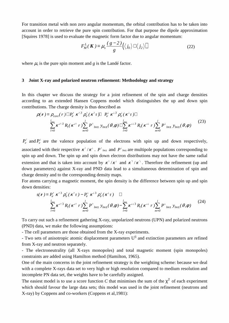
For transition metal with non zero angular momentum, the orbital contribution has to be taken into account in order to retrieve the pure spin contribution. For that purpose the dipole approximation [Squires 1978] is used to evaluate the magnetic form factor due to angular momentum:

( )LM s 0 2

( g 2 )F ( ) j j

gµ −= +K (22)

where µs is the pure spin moment and g is the Landé factor.

3 Joint X-ray and polarized neutron refinement: Methodology and strategy

In this chapter we discuss the strategy for a joint refinement of the spin and charge densities according to an extended Hansen Coppens model which distinguishes the up and down spin contributions. The charge density is thus described as

r r

max max

3 3core

l ll l3 3

l lm lm l lm lml 0 m 0 l 0 m 0

( ) ( r ) P ( ) P ( )

' R ( ' r ) P y ( , ) ' R ( ' r ) P y ( , )

ν ν ν νρ ρ κ ρ κ κ ρ κ

κ κ θ φ κ κ θ φ

↑ ↑ ↑ ↑ ↓ ↓ ↓ ↓

↑ ↑ ↑ ↓ ↓ ↓± ± ± ±

= = = =

= + + +

+∑ ∑ ∑ ∑

r

(23)

↑νP and ↓

νP are the valence population of the electrons with spin up and down respectively,

associated with their respective ↑κ / ↓κ . ±↑

lmP and ±↓

lmP are multipole populations corresponding to spin up and down. The spin up and spin down electron distributions may not have the same radial

extension and that is taken into account by ↑κ / ↓κ and ↑'κ / ↓'κ . Therefore the refinement (up and down parameters) against X-ray and PND data lead to a simultaneous determination of spin and charge density and to the corresponding density maps. For atoms carrying a magnetic moment, the spin density is the difference between spin up and spin down densities:

3 3

3 3

0 0

r r

max maxl ll l

l lm lm l lm lml m 0 l m 0

s( ) P ( ) P ( )

' R ( ' r ) P y ( , ) ' R ( ' r ) P y ( , )

ν ν ν νκ ρ κ κ ρ κ

κ κ θ φ κ κ θ φ

↑ ↑ ↑ ↑ ↓ ↓ ↓ ↓

↑ ↑ ↑ ↓ ↓ ↓± ± ± ±

= = = =

= − +

−∑ ∑ ∑ ∑

r

(24)

To carry out such a refinement gathering X-ray, unpolarized neutrons (UPN) and polarized neutrons (PND) data, we make the following assumptions: - The cell parameters are those obtained from the X-ray experiments. - Two sets of anisotropic atomic displacement parameters Uij and extinction parameters are refined from X-ray and neutron separately. - The electroneutrality (all X-rays monopoles) and total magnetic moment (spin monopoles) constraints are added using Hamilton method (Hamilton, 1965). One of the main concerns in the joint refinement strategy is the weighting scheme: because we deal with a complete X-rays data set to very high or high resolution compared to medium resolution and incomplete PN data set, the weights have to be carefully assigned.

The easiest model is to use a score function C that minimises the sum of the χ2 of each experiment which should favour the large data sets; this model was used in the joint refinement (neutrons and X-ray) by Coppens and co-workers (Coppens et al,1981):

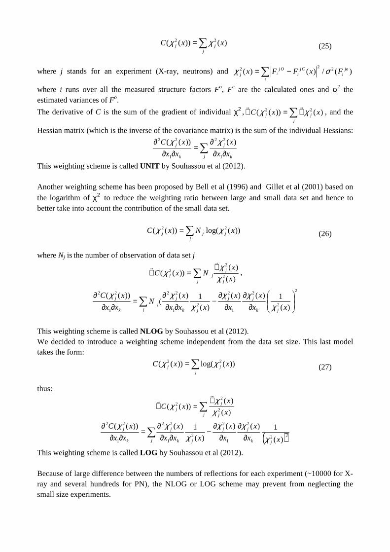
)())(( 22 xxCj

jj ∑= χχ (25)

where j stands for an experiment (X-ray, neutrons) and )(/)()( 222 ∑ −=i

joi

Cji

Ojj FxFFx i σχ

where i runs over all the measured structure factors Fo, Fc are the calculated ones and σ2 the estimated variances of Fo.

The derivative of C is the sum of the gradient of individual χ2 , )())(( 22 xxCj

jj ∑∇=∇ χχ

, and the

Hessian matrix (which is the inverse of the covariance matrix) is the sum of the individual Hessians:

∑ ∂∂∂

=∂∂

∂

j k

j

k

j

xx

x

xx

xC

1

22

1

22 )())(( χχ

This weighting scheme is called UNIT by Souhassou et al (2012). Another weighting scheme has been proposed by Bell et al (1996) and Gillet et al (2001) based on

the logarithm of χ2 to reduce the weighting ratio between large and small data set and hence to better take into account the contribution of the small data set.

))(log())(( 22 xNxCj

jjj ∑= χχ (26)

where Nj is the number of observation of data set j

∑∇

=∇j j

jjj x

xNxC

)(

)())((

2

22

χχ

χ

,

2

2

2

1

2

21

22

1

22

)(

1)()(

)(

1)((

))((

∂∂

∂∂

−∂∂

∂=

∂∂∂

∑xx

x

x

x

xxx

xN

xx

xC

jk

jj

jj k

jj

k

j

χχχ

χχχ

This weighting scheme is called NLOG by Souhassou et al (2012). We decided to introduce a weighting scheme independent from the data set size. This last model takes the form:

))(log())(( 22 xxCj

jj ∑= χχ (27)

thus:

∑∇

=∇j j

jj x

xxC

)(

)())((

2

22

χχ

χ

( )22

2

1

2

21

22

1

22

)(

1)()(

)(

1)())((

xx

x

x

x

xxx

x

xx

xC

jk

jj

jj k

j

k

j

χ

χχχ

χχ∂

∂∂

∂−

∂∂∂

=∂∂

∂∑

This weighting scheme is called LOG by Souhassou et al (2012). Because of large difference between the numbers of reflections for each experiment (~10000 for X-ray and several hundreds for PN), the NLOG or LOG scheme may prevent from neglecting the small size experiments.

To begin the joint refinement, the chosen initial model is the model in which the density is refined against X-ray only using the Hansen Coppens model. For atoms that are supposed to carry a spin density, their multipole populations are split in two for up and down and then refined against both data sets. 4 Charge and spin density of an end-to-end Azido Double Bridged CuII di nuclear complex

(Cu2L2(N3)2). The following reports on preliminary results of the joint charge and spin density refinement of a di copper paramagnetic couple.

4.1 Description of the structure and charge density

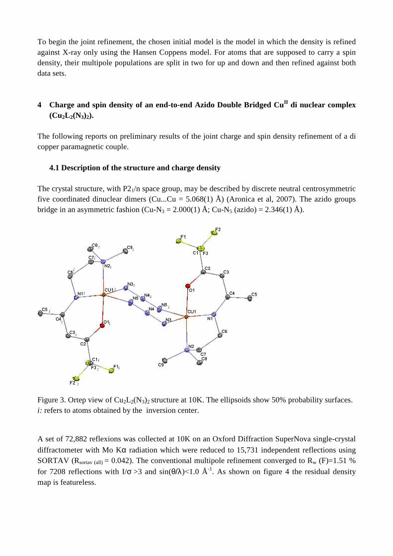
The crystal structure, with P21/n space group, may be described by discrete neutral centrosymmetric five coordinated dinuclear dimers (Cu...Cu = 5.068(1) Å) (Aronica et al, 2007). The azido groups bridge in an asymmetric fashion (Cu-N3 = 2.000(1) Å; Cu-N5 (azido) = 2.346(1) Å).

Figure 3. Ortep view of Cu2L2(N3)2 structure at 10K. The ellipsoids show 50% probability surfaces. i: refers to atoms obtained by the inversion center. A set of 72,882 reflexions was collected at 10K on an Oxford Diffraction SuperNova single-crystal

diffractometer with Mo Kα radiation which were reduced to 15,731 independent reflections using SORTAV (Rsortav (all) = 0.042). The conventional multipole refinement converged to Rw (F)=1.51 %

for 7208 reflections with I/σ >3 and sin(θ/λ)<1.0 Å-1. As shown on figure 4 the residual density map is featureless.

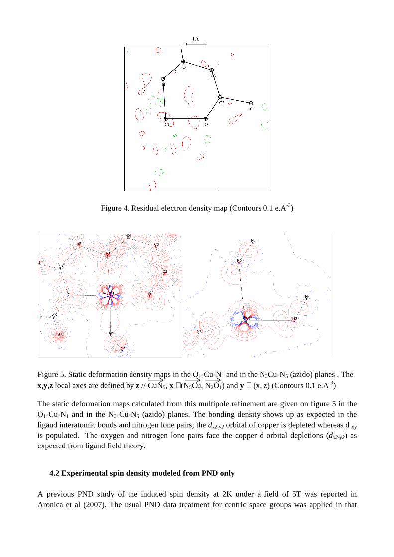
Figure 4. Residual electron density map (Contours 0.1 e.A-3)

Figure 5. Static deformation density maps in the O1-Cu-N1 and in the N3Cu-N5 (azido) planes . The

x,y,z local axes are defined by z // CuN5, x ⊥(N5Cu, N2O1) and y ⊥ (x, z) (Contours 0.1 e.A-3) The static deformation maps calculated from this multipole refinement are given on figure 5 in the O1-Cu-N1 and in the N3-Cu-N5 (azido) planes. The bonding density shows up as expected in the ligand interatomic bonds and nitrogen lone pairs; the dx2-y2 orbital of copper is depleted whereas d xy is populated. The oxygen and nitrogen lone pairs face the copper d orbital depletions (dx2-y2) as expected from ligand field theory.

4.2 Experimental spin density modeled from PND only A previous PND study of the induced spin density at 2K under a field of 5T was reported in Aronica et al (2007). The usual PND data treatment for centric space groups was applied in that

work, i.e. the magnetic structure factors were deduced from the experimental flipping ratios using the FN values calculated from the neutron structure determined at 30K.

Only reflections with |FN|>5.10-12cm were measured in order to avoid contamination due to multiple scattering. In the joint refinement method, the model refinement is performed by comparing the experimental data with the flipping ratios calculated from the model. For a comparison between the results of the joint refinement and those obtained from PND alone, we performed a new treatment of the PND data by refining the model on the set of flipping ratios instead of the FM’s. Because the flipping ratios for (h,k,l) and (h,-k,l) equivalent reflections may be different, the refinement was performed on a set of 212 flipping ratios instead of the 112 unique FM’s. The correction for hydrogen nuclear

spin polarization was also taken into account with HNPf = 0.037 10-12cm for H = 5T and T = 2K (list

of FNP in supplementary material). In Aronica's paper the orbital contribution, calculated using

expression (10) with the value µs(g-2)/g=0.069 µB, was subtracted from the experimental structure factor to obtain the pure spin magnetic structure factor. In order to apply this correction in the flipping ratio refinement, the form factor (<j 0>+<j 2>) for Cu2+ was introduced for the first

monopole. The refinement of the Cu first monopole population (Pv) provided a value of 0.071(6) µB very close to the value fixed in Aronica's paper

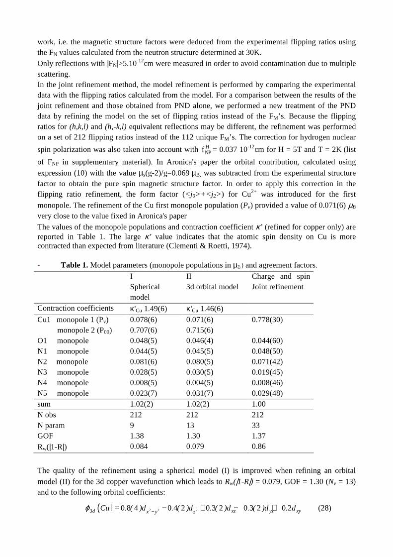
The values of the monopole populations and contraction coefficient κ’ (refined for copper only) are reported in Table 1. The large κ’ value indicates that the atomic spin density on Cu is more contracted than expected from literature (Clementi & Roetti, 1974). - Table 1. Model parameters (monopole populations in µB)and agreement factors.

I Spherical model

II 3d orbital model

Charge and spin Joint refinement

Contraction coefficients κ'Cu 1.49(6) κ'Cu 1.46(6)

Cu1 monopole 1 (Pv) 0.078(6) 0.071(6) 0.778(30) monopole 2 (P00) 0.707(6) 0.715(6) O1 monopole 0.048(5) 0.046(4) 0.044(60) N1 monopole 0.044(5) 0.045(5) 0.048(50) N2 monopole 0.081(6) 0.080(5) 0.071(42) N3 monopole 0.028(5) 0.030(5) 0.019(45) N4 monopole 0.008(5) 0.004(5) 0.008(46) N5 monopole 0.023(7) 0.031(7) 0.029(48) sum 1.02(2) 1.02(2) 1.00 N obs 212 212 212 N param 9 13 33 GOF 1.38 1.30 1.37

Rw(|1-R|) 0.084 0.079 0.86

The quality of the refinement using a spherical model (I) is improved when refining an orbital

model (II) for the 3d copper wavefunction which leads to Rw(|1-R|) = 0.079, GOF = 1.30 (Nv = 13) and to the following orbital coefficients:

( ) 2 2 23 0 8 4 0 4 2 0 3 2 0 3 2 0 2d xz yz xyx y zCu . ( )d . ( )d . ( )d . ( )d . dϕ −= − + − + (28)

where the x, y, z axes have the same definition as in the X-ray study (see Figure 5 caption). The copper multipole populations are constrained during the refinement through their relations with the orbital coefficients as detailed in supplementary materials. The sum of the monopole populations, equal to 1.02(2) µB per asymmetrical unit, provides a value

of 2.02(4) µB/mol for the total induced moment due to spin and orbital contributions. This value is

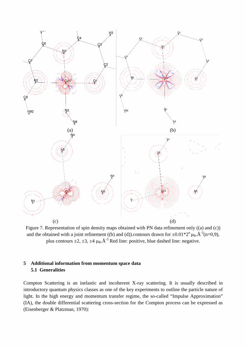
in very good agreement with the experimental magnetization of 1.98 µB/mol from SQUID measurements at 2K under 5 Tesla (Aronica et al, 2007). The section maps of the spin density in the CuO1N1 (x,y) and CuN1N5 (y,z) planes are represented in Figure 7 (a and c).

4.3 Joint refinement

The very first results for the joint refinement were obtained by splitting the charge density model

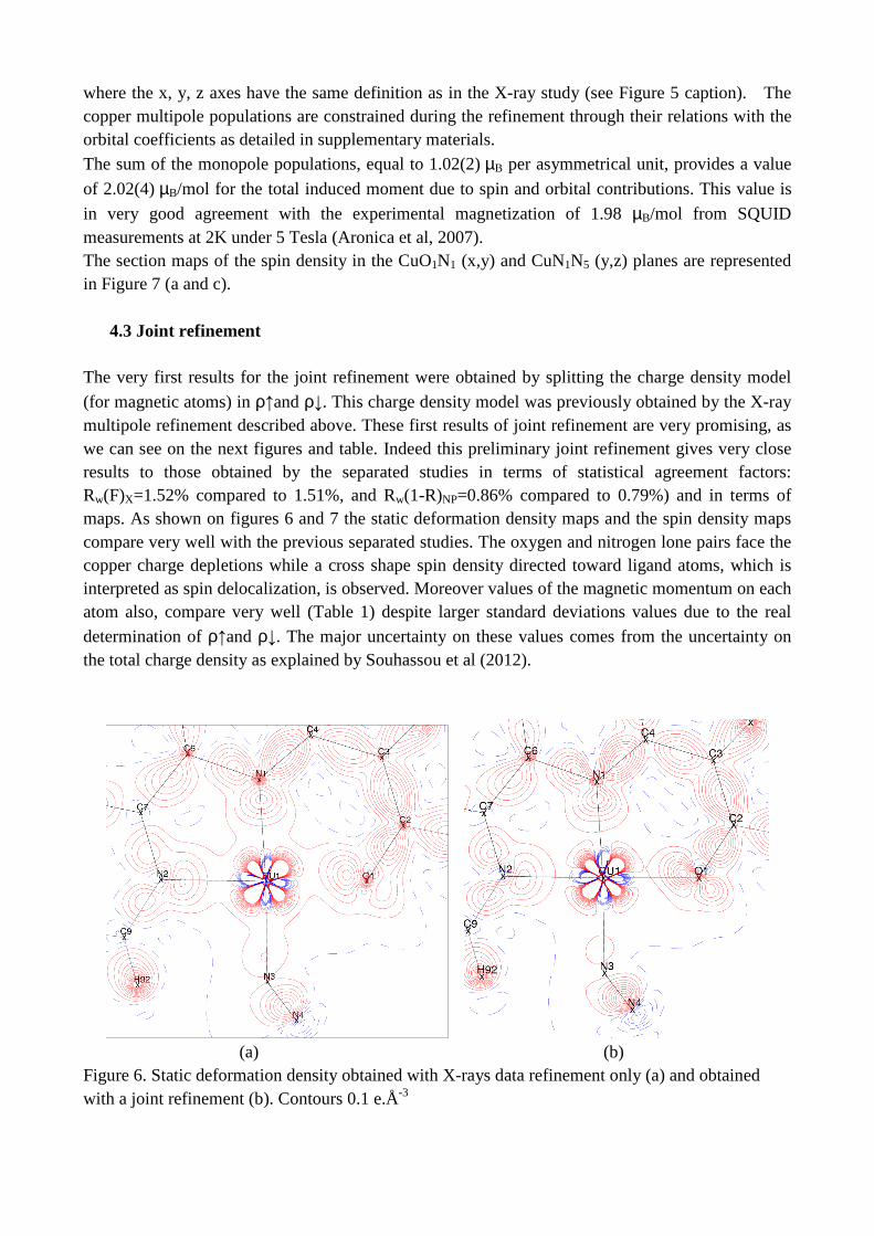
(for magnetic atoms) in ρ↑and ρ↓. This charge density model was previously obtained by the X-ray multipole refinement described above. These first results of joint refinement are very promising, as we can see on the next figures and table. Indeed this preliminary joint refinement gives very close results to those obtained by the separated studies in terms of statistical agreement factors: Rw(F)X=1.52% compared to 1.51%, and Rw(1-R)NP=0.86% compared to 0.79%) and in terms of maps. As shown on figures 6 and 7 the static deformation density maps and the spin density maps compare very well with the previous separated studies. The oxygen and nitrogen lone pairs face the copper charge depletions while a cross shape spin density directed toward ligand atoms, which is interpreted as spin delocalization, is observed. Moreover values of the magnetic momentum on each atom also, compare very well (Table 1) despite larger standard deviations values due to the real

determination of ρ↑and ρ↓. The major uncertainty on these values comes from the uncertainty on the total charge density as explained by Souhassou et al (2012).

(a) (b) Figure 6. Static deformation density obtained with X-rays data refinement only (a) and obtained with a joint refinement (b). Contours 0.1 e.Å-3

(a) (b)

(c) (d) Figure 7. Representation of spin density maps obtained with PN data refinement only ((a) and (c)) and the obtained with a joint refinement ((b) and (d)).contours drawn for ±0.01*2n

µB.Å-3(n=0,9), plus contours ±2, ±3, ±4 µB.Å-3 Red line: positive, blue dashed line: negative.

5 Additional information from momentum space data

5.1 Generalities Compton Scattering is an inelastic and incoherent X-ray scattering. It is usually described in introductory quantum physics classes as one of the key experiments to outline the particle nature of light. In the high energy and momentum transfer regime, the so-called “Impulse Approximation” (IA), the double differential scattering cross-section for the Compton process can be expressed as (Eisenberger & Platzman, 1970):

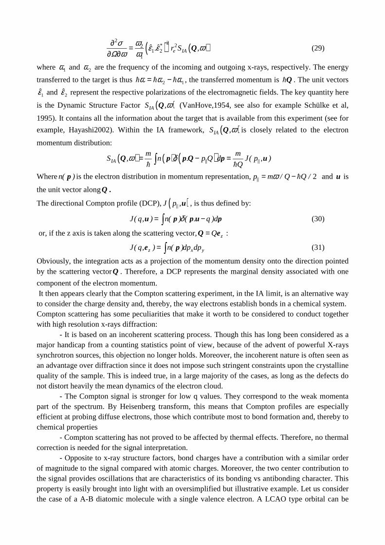
( ) ( )2 2 22

1 21

*e IAˆ ˆ. r S ,

ωσ ε ε ωΩ ω ω∂ =

∂ ∂Q (29)

where 1ω and 2ω are the frequency of the incoming and outgoing x-rays, respectively. The energy

transferred to the target is thus 12 ωωω ℏℏℏ −= , the transferred momentum is Qℏ . The unit vectors

1ε and 2ε represent the respective polarizations of the electromagnetic fields. The key quantity here

is the Dynamic Structure Factor ( )IAS ,ωQ (VanHove,1954, see also for example Schülke et al,

1995). It contains all the information about the target that is available from this experiment (see for

example, Hayashi2002). Within the IA framework, ( )IAS ,ωQ is closely related to the electron

momentum distribution:

( ) ( ) ( )IAm m

S , n . p Q d J( p , )Q

ω δ= − =∫Q p p Q p u ℏ ℏ

Wheren( )p is the electron distribution in momentum representation, 2p m / Q Q /ω= − ℏ and u is

the unit vector alongQ .

The directional Compton profile (DCP),( )J p ,u , is thus defined by:

J( q, ) n( ) ( . q )dδ= −∫u p p u p (30)

or, if the z axis is taken along the scattering vector, zQ=Q e :

z x yJ( q, ) n( )dp dp= ∫e p (31)

Obviously, the integration acts as a projection of the momentum density onto the direction pointed by the scattering vectorQ . Therefore, a DCP represents the marginal density associated with one

component of the electron momentum. It then appears clearly that the Compton scattering experiment, in the IA limit, is an alternative way to consider the charge density and, thereby, the way electrons establish bonds in a chemical system. Compton scattering has some peculiarities that make it worth to be considered to conduct together with high resolution x-rays diffraction:

- It is based on an incoherent scattering process. Though this has long been considered as a major handicap from a counting statistics point of view, because of the advent of powerful X-rays synchrotron sources, this objection no longer holds. Moreover, the incoherent nature is often seen as an advantage over diffraction since it does not impose such stringent constraints upon the crystalline quality of the sample. This is indeed true, in a large majority of the cases, as long as the defects do not distort heavily the mean dynamics of the electron cloud.

- The Compton signal is stronger for low q values. They correspond to the weak momenta part of the spectrum. By Heisenberg transform, this means that Compton profiles are especially efficient at probing diffuse electrons, those which contribute most to bond formation and, thereby to chemical properties

- Compton scattering has not proved to be affected by thermal effects. Therefore, no thermal correction is needed for the signal interpretation.

- Opposite to x-ray structure factors, bond charges have a contribution with a similar order of magnitude to the signal compared with atomic charges. Moreover, the two center contribution to the signal provides oscillations that are characteristics of its bonding vs antibonding character. This property is easily brought into light with an oversimplified but illustrative example. Let us consider the case of a A-B diatomic molecule with a single valence electron. A LCAO type orbital can be

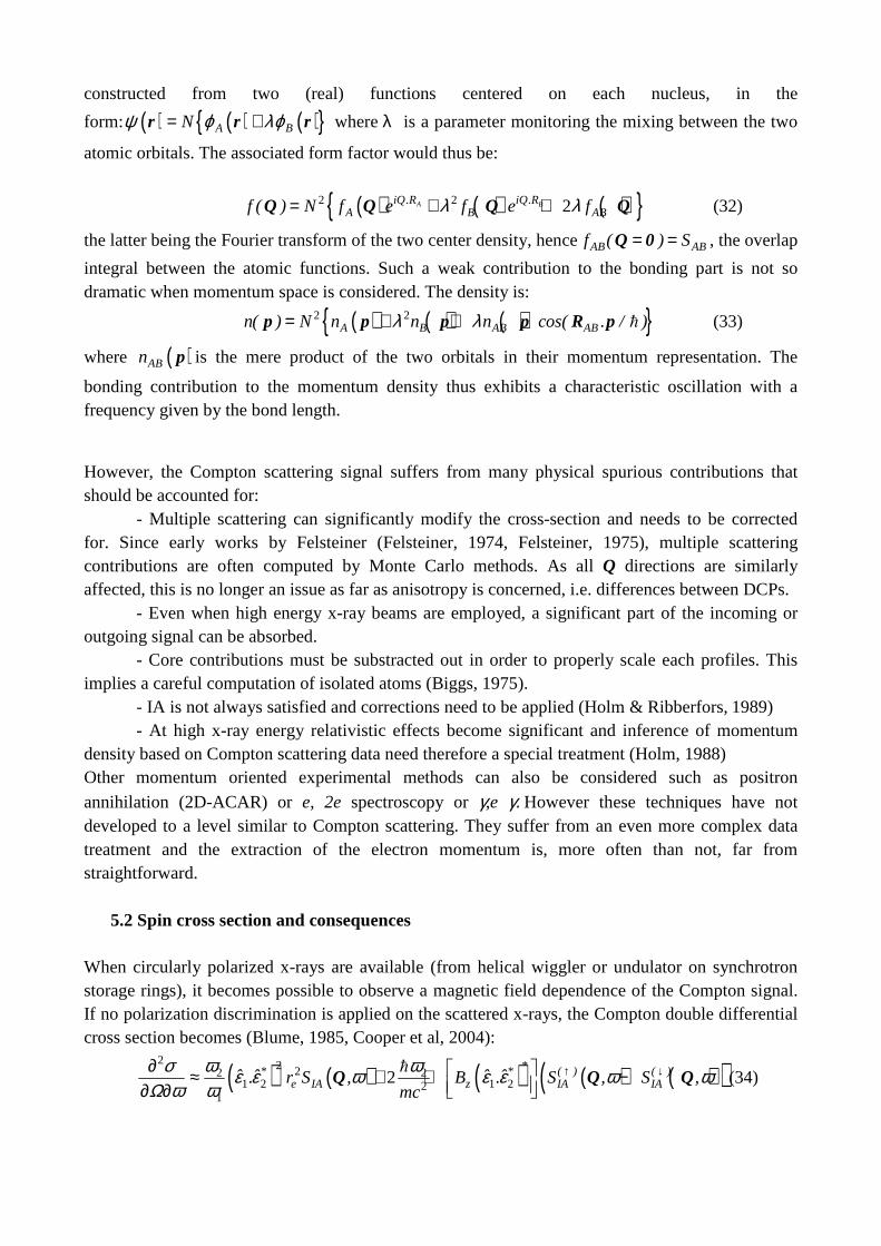
constructed from two (real) functions centered on each nucleus, in the

form: ( ) ( ) ( ) A BNψ ϕ λϕ= +r r r where λ is a parameter monitoring the mixing between the two

atomic orbitals. The associated form factor would thus be:

( ) ( ) ( ) 2 2 2A BiQ.R iQ.RA B ABf ( ) N f e f e fλ λ= + +Q Q Q Q (32)

the latter being the Fourier transform of the two center density, henceAB ABf ( ) S= =Q 0 , the overlap

integral between the atomic functions. Such a weak contribution to the bonding part is not so dramatic when momentum space is considered. The density is:

( ) ( ) ( ) 2 2A B AB ABn( ) N n n n cos( . / )λ λ= + +p p p p R p ℏ (33)

where ( )ABn p is the mere product of the two orbitals in their momentum representation. The

bonding contribution to the momentum density thus exhibits a characteristic oscillation with a frequency given by the bond length.

However, the Compton scattering signal suffers from many physical spurious contributions that should be accounted for:

- Multiple scattering can significantly modify the cross-section and needs to be corrected for. Since early works by Felsteiner (Felsteiner, 1974, Felsteiner, 1975), multiple scattering contributions are often computed by Monte Carlo methods. As all Q directions are similarly affected, this is no longer an issue as far as anisotropy is concerned, i.e. differences between DCPs.

- Even when high energy x-ray beams are employed, a significant part of the incoming or outgoing signal can be absorbed.

- Core contributions must be substracted out in order to properly scale each profiles. This implies a careful computation of isolated atoms (Biggs, 1975).

- IA is not always satisfied and corrections need to be applied (Holm & Ribberfors, 1989) - At high x-ray energy relativistic effects become significant and inference of momentum

density based on Compton scattering data need therefore a special treatment (Holm, 1988) Other momentum oriented experimental methods can also be considered such as positron annihilation (2D-ACAR) or e, 2e spectroscopy or γ,e γ. However these techniques have not developed to a level similar to Compton scattering. They suffer from an even more complex data treatment and the extraction of the electron momentum is, more often than not, far from straightforward.

5.2 Spin cross section and consequences When circularly polarized x-rays are available (from helical wiggler or undulator on synchrotron storage rings), it becomes possible to observe a magnetic field dependence of the Compton signal. If no polarization discrimination is applied on the scattered x-rays, the Compton double differential cross section becomes (Blume, 1985, Cooper et al, 2004):

( ) ( ) ( ) ( ) ( )( )2 2 22 2

1 2 1 221

2** * ( ) ( )

e IA z IA IAˆ ˆ ˆ ˆ. r S , B . S , S ,mc

ω ωσ ε ε ω ε ε ω ωΩ ω ω

↑ ↓∂ ≈ + ℑ − ∂ ∂ Q Q Q

ℏ(34)

where the orbital momentum contribution has been neglected and only lowest order terms have been kept. Thus, in addition to the previous Compton scattering signal, one observes a spin dependent contribution with the dynamic structure factor:

( ) ( )( ) ( )IA

m mS , n , ( . p Q )d J ( p , )

Qω δ↑ ↑= ↑ − =∫Q p p Q p u

ℏ ℏ (35)

In the case of large systems, or unit cells containing many atoms, the interpretation of experimental DCP becomes difficult because, in momentum representation, all atomic sites contributions are superimposed. This is obviously a handicap as all our chemical intuition is based upon a position space description of interacting atoms. However, when it comes to magnetic systems, only unpaired electrons contribute significantly to the signal and a very limited number of atoms need to be included in the model. Polarized neutron diffraction and magnetic Compton scattering can thus be seen as two techniques probing similar parts of the electron distribution. It should nevertheless be noted that, since the magnetic signal is obtained by means of subtraction between two opposite magnetic field directions, all atoms contribute to the background noise. This fact severely limits the number of magnetic systems that can be tackled by that kind of probe.

Two additional points differentiate the magnetic Compton scattering technique from polarized neutron diffraction. First, because of its direct link to momentum space representation, MCP measurements are useless for the study of purely antiferromagnets. Second, owing to a significant different polarization dependence, the spin contribution can in principle be isolated from the orbital signal.

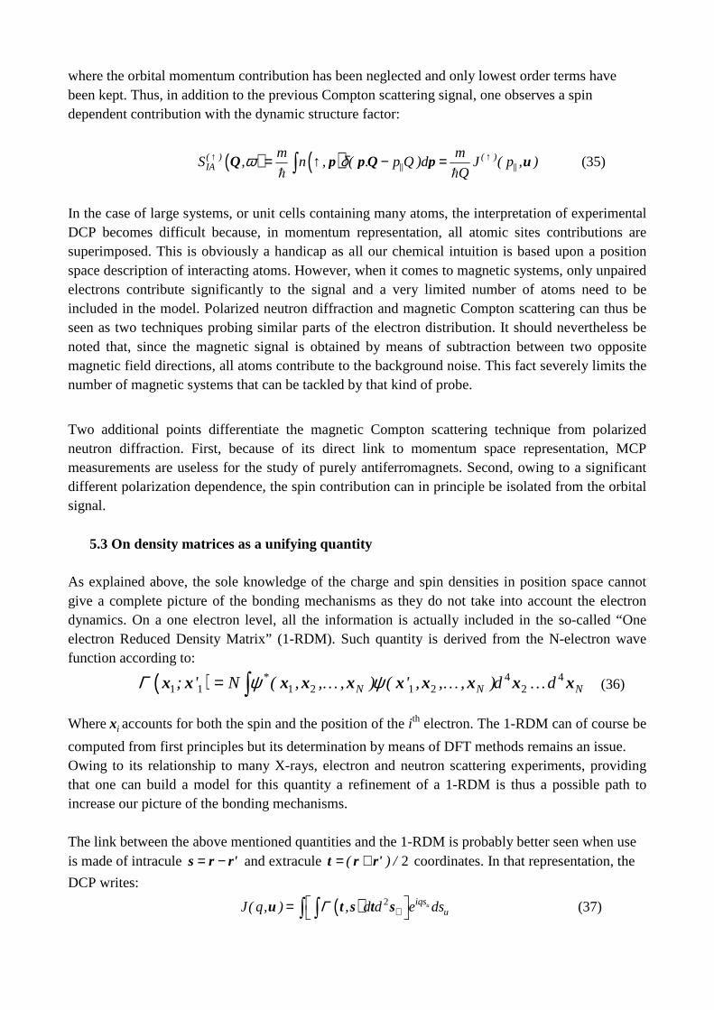
5.3 On density matrices as a unifying quantity

As explained above, the sole knowledge of the charge and spin densities in position space cannot give a complete picture of the bonding mechanisms as they do not take into account the electron dynamics. On a one electron level, all the information is actually included in the so-called “One electron Reduced Density Matrix” (1-RDM). Such quantity is derived from the N-electron wave function according to:

( ) 4 41 1 1 2 1 2 2

*N N N; ' N ( , , , ) ( ' , , , )d d= ∫x x x x x x x x x x… … …Γ ψ ψ (36)

Where ix accounts for both the spin and the position of the i th electron. The 1-RDM can of course be

computed from first principles but its determination by means of DFT methods remains an issue. Owing to its relationship to many X-rays, electron and neutron scattering experiments, providing that one can build a model for this quantity a refinement of a 1-RDM is thus a possible path to increase our picture of the bonding mechanisms. The link between the above mentioned quantities and the 1-RDM is probably better seen when use is made of intracule = −s r r' and extracule 2( ) /= +t r r' coordinates. In that representation, the

DCP writes:

( ) 2 uiqsuJ( q, ) , d d e dsΓ ⊥ = ∫ ∫u t s t s (37)

where us .= s u and ⊥ = ⊗s s u.

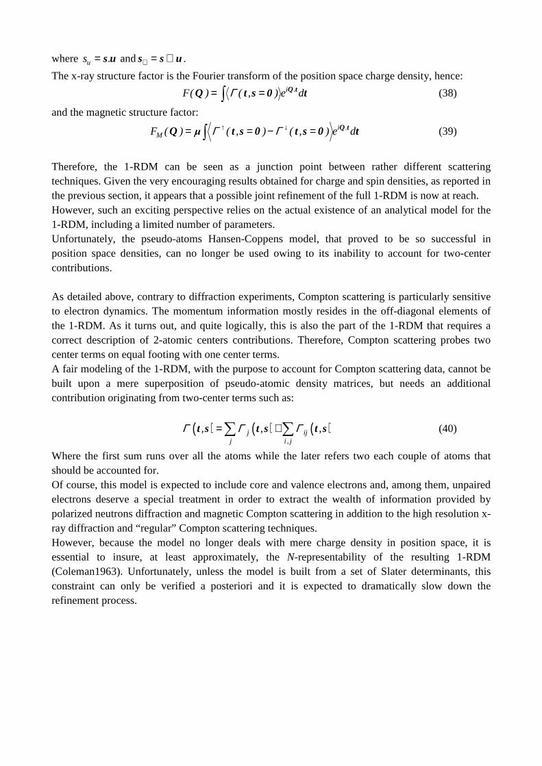
The x-ray structure factor is the Fourier transform of the position space charge density, hence: i .F( ) ( , ) e dΓ= =∫Q tQ t s 0 t (38)

and the magnetic structure factor: i .

MF ( ) ( , ) ( , ) e dΓ Γ↑ ↓= = − =∫Q tQ µ t s 0 t s 0 t (39)

Therefore, the 1-RDM can be seen as a junction point between rather different scattering techniques. Given the very encouraging results obtained for charge and spin densities, as reported in the previous section, it appears that a possible joint refinement of the full 1-RDM is now at reach. However, such an exciting perspective relies on the actual existence of an analytical model for the 1-RDM, including a limited number of parameters. Unfortunately, the pseudo-atoms Hansen-Coppens model, that proved to be so successful in position space densities, can no longer be used owing to its inability to account for two-center contributions. As detailed above, contrary to diffraction experiments, Compton scattering is particularly sensitive to electron dynamics. The momentum information mostly resides in the off-diagonal elements of the 1-RDM. As it turns out, and quite logically, this is also the part of the 1-RDM that requires a correct description of 2-atomic centers contributions. Therefore, Compton scattering probes two center terms on equal footing with one center terms. A fair modeling of the 1-RDM, with the purpose to account for Compton scattering data, cannot be built upon a mere superposition of pseudo-atomic density matrices, but needs an additional contribution originating from two-center terms such as:

( ) ( ) ( )j ijj i , j

, , ,Γ Γ Γ= +∑ ∑t s t s t s (40)

Where the first sum runs over all the atoms while the later refers two each couple of atoms that should be accounted for. Of course, this model is expected to include core and valence electrons and, among them, unpaired electrons deserve a special treatment in order to extract the wealth of information provided by polarized neutrons diffraction and magnetic Compton scattering in addition to the high resolution x-ray diffraction and “regular” Compton scattering techniques. However, because the model no longer deals with mere charge density in position space, it is essential to insure, at least approximately, the N-representability of the resulting 1-RDM (Coleman1963). Unfortunately, unless the model is built from a set of Slater determinants, this constraint can only be verified a posteriori and it is expected to dramatically slow down the refinement process.

Acknowledgement: .

This work has been supported by l'Agence Nationale de la Recherche (CEDA Project) and M.D. thanks

C.N.R.S for PhD fellowship

References Aronica, C., Jeanneau, E., El Moll, H., Luneau, D., Gillon, B., Goujon, A., Cousson, A., Carvajal, M. A., & Robert, V. (2007). Chem. Eur. J. 13, 3666–3674 Aronica C., Chumakov Y., Jeanneau, E., Luneau D., Neugebauer P., Barra A.L., Gillon B., Goujon

A., Cousson A., Tercero J., Ruiz E., (2008) Chem. Eur. J. 14, 9540 – 9548

Becker, P. & Coppens, P. (1985). Acta Cryst. A 41, 177–182. Bell, B., Burke, J., & Schumitzky, A. (1996). Comp. Stat. And Data Anal 22, 119–135 Biggs F., Mendelsohn L.B., Mann J.B. (1975) Atomic Data and Nuclear Data Tables 16, 201-309 Blume M., J. (1985) Appl. Phys. 57, 3615 . Brown, P. J., Forsyth, J. B., & Mason, R. (1980). Phil. Trans. R. Soc. Lond. B 290, 481–495. Bytheway, I., Grimwood, D., Figgis, B., Chandler, G., & Jayatilaka, D. (2002a). Acta Cryst. A 58, 244–251 Bytheway, I., Grimwood, D., & Jayatilaka, D. (2002b). Acta Cryst. A 58, 232–243. Blessing R.H. and Lecomte C. (1991) in "The application of charge density research to chemistry and drug design", NATO Adv. Studies, G.A. Geffrey and J.F. Piniella eds, 90-120. Clementi, E. & Roetti, C. (1974). Atomic Data and Nuclear Data Tables 14, 177–478. Coleman A.J.(1963) Review of Modern Physics 35, 668-687 Cooper, M. J., Mijnarends, P. E., Shiotani, N., Sakai, N., & Bansil, A. (2004). X-ray Compton scattering. Oxford University Press. Coppens, P., Boehme, R., Price, P. F., & Stevens, E. D. (1981). Acta Cryst. A 37, 857–863. Coppens P. & Becker P. (1992) Analysis of charge and spin densities. Int. Tables for X-ray Crystallography, Vol.C, 627-245. Coppens, P. (1997). X-Ray Charge Densities and Chemical Bonding (International Union of Crystallography Texts on Crystallography , No 4). Oxford University Press.

Eisenberger P. & Platzman P.M.(1970) Compton Scattering of X Rays from Bound Electrons. Phys. Rev. A 2, 415-423, Felsteiner J. & Pattison P., (1975) Nuclear Instruments and Methods, 124, 449-453 Felsteiner J. & Pattison P., Cooper M., (1974) Philosophical Magazine 30, 537-548 Gillet, J.-M., Becker, P. J., & Cortona, P. (2001). Phys. Rev. B 63, 235115 Grimwood, D., Bytheway, I., & Jayatilaka, D. (2003). J. Comput. Chem. 24, 470–483. Grimwood, D. & Jayatilaka, D. (2001). Acta Cryst. A 57, 87–100. Hamilton, W. C. (1965). Acta Cryst. 18, 502–510 Hansen, N. K. & Coppens, P. (1978). Acta Cryst. A 34, 909–921. Hayashi, H., Udagawa, Y., Gillet, J.-M., Caliebe, W., & Kao, C.-C. (2002). Chemical Applications of Synchrotron Radiation volume 12 of Advanced Series in Physical Chemistry chapter 18. World Scientific publishing, Singapore. Hirshfeld F.L. (1977) Isr. J. Chem. 16, 226-229. Holladay, A., Leung, P., & Coppens, P. (1983). Acta Cryst. A 39, 377–387. Holm P. & Ribberfors R. (1989) Phys. Rev. A 40, 6251 Holm P. (1988) Phys. Rev. A 37, 3706 Howard, S., Huke, J., Mallinson, P., & Frampton, C. (1994). Phys. Rev. B 49, 7124–7136. Jayatilaka, D. & Grimwood, D. J. (2001). Acta Cryst. A 57, 76–86. Lewis, J., Schwarzenbach, D., & Flack, H. (1982). Acta Cryst. A 38, 733–739. Massa, L., Goldberg, M., Frishberg, C., Boehme, R., & Placa, S. (1985). Phys. Rev. Lett., 55, 622–625. Sakai N.& Ôno K.(1976) Phys. Rev. Lett.37, 351-353 Schülke W., Schmitz J.R., Schulte-Schrepping H. & Kaprolat A. (1995) Phys. Rev. B 52, 11721-11732, Souhassou M., Deutsch M., Claiser N., Pillet S., Lecomte C., Ciumakov Y., Gillon B. and Gillet J-M (2012) Acta Cryst A in preparation.

Squires G. L. (1978), in Introduction to the Theory of Thermal Neutron Scattering, University Press, Cambridge, p.139 Tanaka, K. (1988). Acta Cryst. A, 44, 1002–1008.

Van Hove L. (1954) Phys. Rev. 95, 249-262,

Supplementary materials

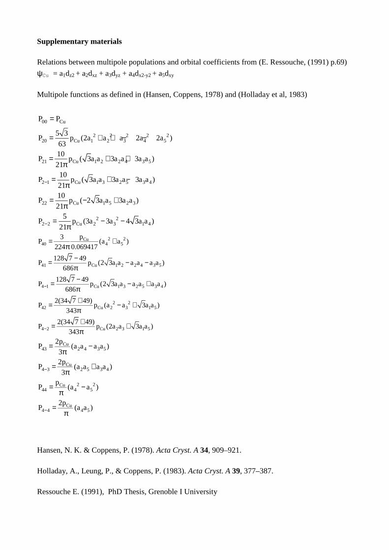
Relations between multipole populations and orbital coefficients from (E. Ressouche, (1991) p.69)

ψCu = a1dz2 + a2dxz + a3dyz + a4dx2-y2 + a5dxy

Multipole functions as defined in (Hansen, Coppens, 1978) and (Holladay et al, 1983)

00 CuP P=

2 2 2 2 220 Cu 1 2 3 4 5

5 3P p (2a a a 2a 2a )

63= + + − −

21 Cu 1 2 2 4 3 510

P p ( 3a a 3a a 3a a )21

= + +π

2 1 Cu 1 3 2 5 3 4

10P p ( 3a a 3a a 3a a )

21− = + −π

22 Cu 1 5 2 3

10P p ( 2 3a a 3a a )

21= − +

π 2 2

2 2 Cu 2 3 1 45

P p (3a 3a 4 3a a )21− = − −

π 2 2Cu

40 4 5p3

P (a a )224 0.069417

= +π

41 Cu 1 2 2 4 3 5

128 7 49P p (2 3a a a a a a )

686

−= − −π

4 1 Cu 1 3 2 5 3 4

128 7 49P p (2 3a a a a a a )

686−−= − +π

2 2

42 Cu 2 3 1 52(34 7 49)

P p (a a 3a a )343

+= − +π

4 2 Cu 2 3 1 5

2(34 7 49)P p (2a a 3a a )

343−+= +π

Cu43 2 4 3 5

2pP (a a a a )

3= −

π Cu

4 3 2 5 3 42p

P (a a a a )3− = +π

2 2Cu44 4 5

pP (a a )= −

π

Cu4 4 4 5

2pP (a a )− =

π

Hansen, N. K. & Coppens, P. (1978). Acta Cryst. A 34, 909–921. Holladay, A., Leung, P., & Coppens, P. (1983). Acta Cryst. A 39, 377–387. Ressouche E. (1991), PhD Thesis, Grenoble I University