Embed Size (px)
Citation preview

Computational Fluid Dynamics
Dr.Eng. Reima IwatsuPhone: 0355 69 4875
e-mail: [email protected] Building Room 53-107
Time Summer TermLecture: Tuesday 7:30-9:00 (every two weeks) LG4/310Exercise: Tuesday 7:30-9:00 (every four weeks)LG4/310
Evaluation: 10% Attendance 90% Exercise and Report 90%Speeking time Tuesday 9:00-10:30
Lehrstuhl Aerodynamik und Strömungslehre (LAS)Fakultät 3, Maschinenbau, Elektrotechnik und Wirtschaftsingenieurwesen
Brandenburgische Technische Universität CottbusKarl Liebknecht-Straße 102,D-03046 Cottbus

Terminplanung für die Vorlesung „Computational Fluid Dynamics“(Di., 7:30 – 9:00 Uhr, LG 4 Raum 310)
• Date Contents of the lecture• 3. 4. 2001 Introduction
The mathematical nature of the flow equations• 17. 4. 2001 Finite Difference Method (FDM)
Finite Element Method (FEM)Finite Volume Method (FVM), Fourier/Spectral method
• 24. 4. 2001 Exercise• 8. 5. 2001 Time integration, Stability analysis• 22. 5. 2001 Iterative methods for algebraic systems
Convection-diffusion equation• 29. 5. 2001 Exercise• 5. 6. 2001 Incompressible Navier Stokes(NS) equations
Some remarks on incompressible fows• 12. 6. 2001 Heat and fluid flow
Turbulence modelGrid generation
• 19. 6. 2001 Exercise• 26. 6. 2001 Example CFD results • 3. 7. 2001 Lecture from Dr.Ristau•

Contents of the lecture
Mathematical Property of the PDEs1 Introduction2 The Mathematical Nature of the Flow Equations Various Discretization Method3 Finite Difference Method (FDM)4 Finite Element Method (FEM)5 Finite Volume Method (FVM)6 Fourier/Spectral MethodNumerical Method for Time Marching and System of Equations7 Time Integration 8 Stability Analysis9 Iterative Methods for Algebraic Systems10 Convection-Diffusion EquationIncompressible Flows11 Incompressible Navier Stokes(NS) Equations12 Some Remarks on Incompressible Fows13 Heat and Fluid Flow14 Turbulence ModelGrid Generation / CFD Examples 15 Grid Generation16 Example CFD Results17 Lecture on Applicational Computation (Dr. Ristau)

Contents of the lecture for today• 1 Introduction• 1.1 Introductnion
– 1.1.1 Motivation– 1.1.2 Computational Fluid Dynamics: What is it?– 1.1.3 The Role of CFD in Modern Fluid Dynamics– 1.1.4 The Objective of This Course
• 1.2 The Basic Equations of Fluid Dynamics– 1.2.1 Fluid and Flow– 1.2.2 Mathematical Model– 1.2.3 Conservation Law– 1.2.4 The Continuity Equation– 1.2.5 The Momentum Equation: Navier-Stokes Equations– 1.2.6 The Energy Equation– 1.2.7 Thermodynamic Considerations– 1.2.8 Submodel
• 2 The Mathematical Nature of the Flow Equatnions• 2.1 Linear Partical Differential Equations(PDEs)
– 2.1.1 Classification of the Second Order Linear PDEs– 2.1.2 General Behaviour of the Different Classes of PDEs
• 2.2 The Dynamic Levels of Approximation – 2.2.1 Inviscid Flow Model: Euler Equations– 2.2.2 Parabolized Navier-Stokes Equations, Boundary Layer Approximation– 2.2.3 Potential Flow Model, Incompressible Fluid Flow Model

1.1 IntroductionMotivation: Why should you be motivated to learn CFD?
The flowfield over a supersonic blunt-nosed body Artist's conception of next generation supersonic aircraft

Vehicle aerodynamics, combustion and DNS of turbulence

Computational Fluid Dynamics
• Computational Fluid Dynamics (CFD) is a discipline that solves aset of equations governing the fluid flow over any geometrical configuration. The equations can represent steady or unsteady,compressible or incompressible, and inviscid or viscous flows,including nonideal and reacting fluid behavior. The particularform chosen depends on the intended application. The state of theart is characterized by the complexity of the geometry, the flow physics, and the computer time required to obtain a solution.
• http://fmad-www.larc.nasa.gov/aamb/• Fluid Mechanics and Acoustics Division• NASA Langley Research Center in Hampton, VA.

Computational Fluid Dynamics: What is it?• The physical aspects of any fluid flow are governed by the following
fundamental principles:(a) mass is conserved (b) F = ma (Newton‘s second law)(c) energy is conserved.
• These fundamental principles are expressed in terms of mathematical equations (partial differential equations).
• CFD is the art of replacing the governing equations of fluid flow with numbers, and advancing these numbers in space and/or time to obtain a final numerical description of the complete flow field of interest.
• The high-speed digital computer has allowed the practical growth of CFD.

The Role of CFD in Modern Fluid Dynamics
Pureexperiment
Puretheory
ComputationalFluid
dynamicsFig. The “three dimensions“ of
fluid dynamics
• A new „third approach“.• Equal partner, but never replace either.

The Objective of This Course
• To whom:
The completely uninitiated student
• To provide what:
(a) an understanding of the governing equations(b) some insight into the philosophy of CFD(c) a familiarity with various popular solution techniques;(d) a working vocabulary in the discipline
• At the conclusion of this course:
will be well prepared to understand the literature in this field,to follow more advanced lecture series,and to begin the application of CFD to your special areas of concern.
I I hopehope......

1.2 The Basic Equations of Fluid DynamicsFluid and Flow
Gas, air, fuel, oxigen, CO2
Fluid: Liquid water, oil, liquid metal that flows(Solid) (geophysical flows)

Eulerian and Lagrangian framework
Eulerian description of the flow
the velocity of the fluid u at the position x at time tu (x , t )
Lagrangian labelsthe state and motion of the point particles
a = (a1,a2,a3) Lagrangian labelsu (x , t ) = u ( X (a, t ) , t ) = U (a, t )
u (x , t )
U (a, 0 )b
U (a, t )
a

Mathematical ModelFinite Control VolumeA closed volume in a finite region of the flow: a controle volume V; a controle surface S, closed surface which bounds the volume
fixd in space moving with the fluid
Infinitesimal Fluid ElementAn infinitesimally small fluid element with a volume dV
Control volume V
Control surface S S
V
volume dV

The Material Derivative
The velocity of a point particle = the rate of change of its position X
substantial, material, or convective derivative and is denoted by D/Dt
The Lagrangian set (a, t ) and the Eulerian set (x , t )The relationship between the partial derivatives of a function f
The chain rule
(material (temporal & spatial derivativesderivative) with respect to the Eulerian variables)

The Continuity EquationControl Volume Fixed in Space Physical principle: Mass is conserved.
(Integral form)
Gauss Divergence Theorem

The Continuity Equation (continued)Control Volume Moving with the Fluid
The relationship between the divergenceof Vand dV
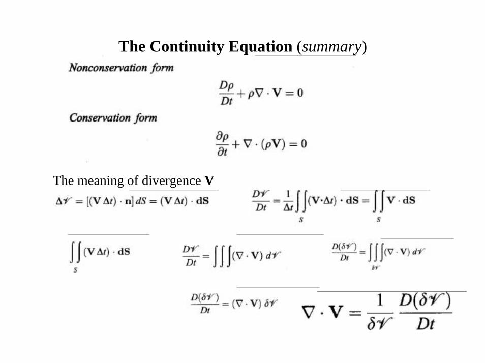
The Continuity Equation (summary)
The meaning of divergence V
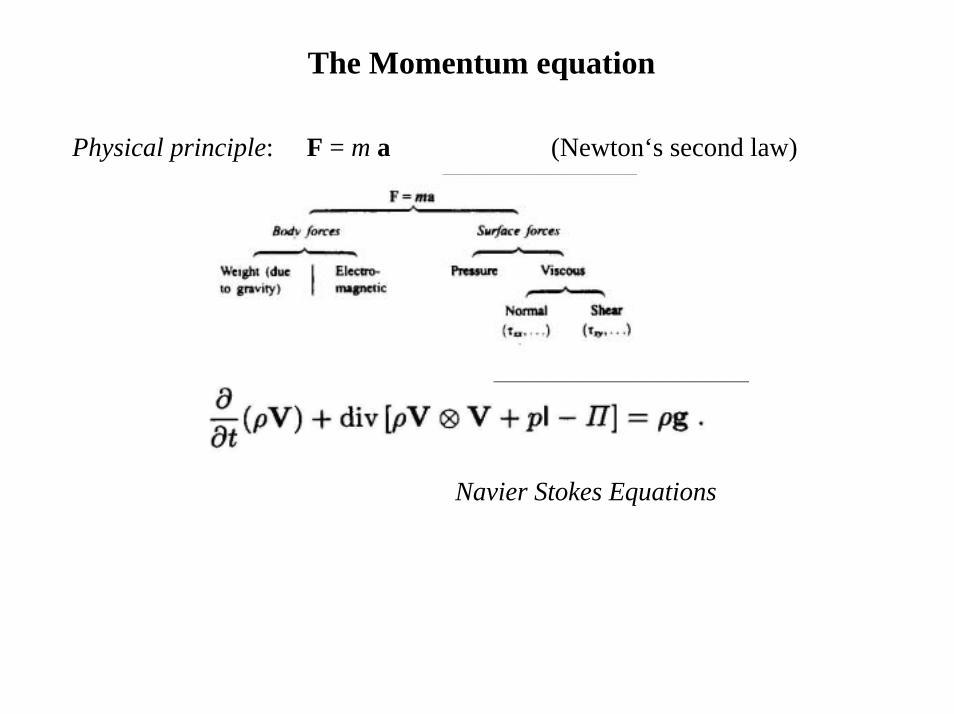
The Momentum equation
Physical principle: F = m a (Newton‘s second law)
Navier Stokes Equations

The Momentum equation

The Energy EquationPhysical principle: Conservation of energy
E: total energy (= e + V 2/2 ) , e: internal energy

Thermodynamic ConsiderationsUnknown flow-field variables: /rho, p, u, v, w, E( or e) Closure conditions for state variables
( e: specific internal energy, s: entropy, p: pressure, /rho: density, T: temperature)
Equation of StateIdeal Gas (a perfect gas)
pV = nR T ( p = ¥rho R T ) (1)V: volume, n:number of kilomoles,R=8.134 KJ: Universal Gas Constant, T: temperature [K].
pv = RT, R = R / w( p = ¥rho RT ) (1#)v : specific volume (=V/m, V: Volume, m: mass. v=1/ ¥rho )w: relative molecular mass, m = n w,R: Specific Gas Constant.
a thermodynamic relatione = e(T,p) (2)
a perfect gase = cvT (2#)
cv: spesific heat at constant volume

2 The Mathematical Nature of the FlowEquatnions
2.1 Linear Partial Differential Equations (PDEs)
Second Order PDEs
Navier Stokes Equations
Second Order Linear PDEs

2.1.1 Classification of the Second Order Linear PDEs
• F(x,y)aFxx + bFxy + cFyy +dFx + eFy + g = 0
b2 – 4ac > 0 hyperbolic
b2 – 4ac = 0 parabolicb2 – 4ac < 0 elliptic

2.1.2 General Behaviour of the Different Classes ofPDEs
• Hyperbolic Equations• Characteristic curves
P
y
a
b
c
Region IInfluenced by point p-Region of influence-
Initial data upon which p depends
Region influenced by point c
Region IIDomain of influence
Right-running characteristic
Left-running characteristic
x

Hyperbolic Equations
(x,y,z)
Characteristic surface
P Volume influenced by point pVolume which influences
point p
y
Initial data in the yz plane upon which p
depends
x
z

Parabolic Equations• Only one characteristic direction,• Marching-type solutions
y Boundary conditions knownc d
Initial data line Pa Region
influenced by P
Boundary conditions known b
x
y y
x=0 x=t

Elliptic Equations
• No limited regions of influence;• information is propagated everywhere in all directions (at once).
yb c
a b x
• Boundary conditions• A specification of the dependent variables along the boundary. Dirichlet condition• A specification of derivatives of the dependent variables along the boundary. Neumann
condition• A mix of both Dirichlet and Neumann conditions.
P

2.2.1 Inviscid Flow Model: Euler EquationsSteady inviscid supersonic flows
Wave equation
2.2 The Dynamic Levels of Approximation

2.2.2 Parabolized Navier-Stokes Equations, Boundary Layer Approximation
Unsteady thermal conduction
Boundary-layer flows
Parabolized viscous flows

2.2.3 Potential Flow Model, Incompressible Fluid Flow Model
Physical picture consistent with the behavior of elliptic equationsPotential Flow: Steady, subsonic, inviscid flow
Flow over an airfoil
Incompressible Fluid Flow: the Mach number M = V/c 0
Flow over a cylinder cylinder

Discretization techniques route mapPDFs System of allgebraic equations
Finite Difference Method (FDM)
Basic derivations
Finite Element Method (FEM)
Finite Volume Method (FVM)
Fourier /Spectral Method
Discretization errors
Time integration
Initial value problem
Types of solutions:
Explicit and implicit
Stability analysis
Iterative methods
Boundary value problemI.V.&B.V. problem

2 Finite Difference Method2.1 Basic Concept
> to discretize the geometric domain > to define a grid> a set of indices (i,j) in 2D, (i,j,k) in 3D> grid node values

The definition of a derivative

2.2 Approximation of the first derivative2.2.1 Taylor series expansion
Expansion at xi+1
Expansion at xi-1
Using eq. at both xi+1 and xi-1
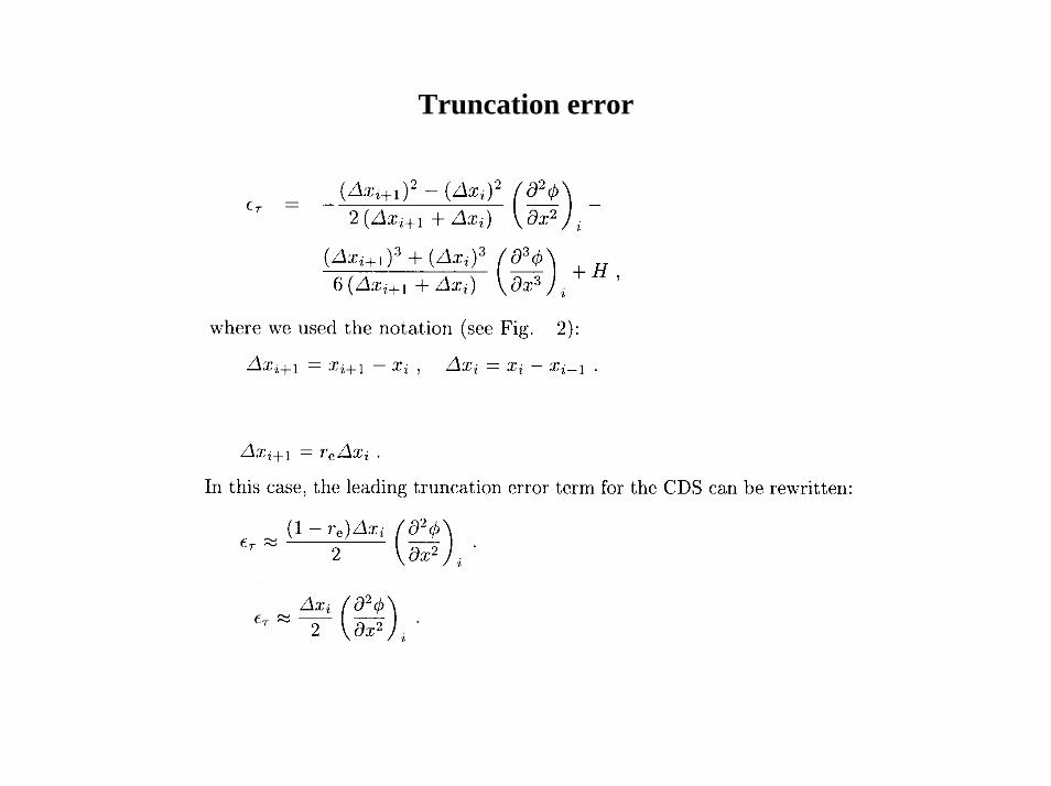
Truncation error

The Forward (FDS), backward (BDS) and central difference (CDS)
Approximations truncating the series
Truncation errors
>for small spacing the leading term is the dominant one>The order of approximation m, m-th order accuracy
Second order approximation
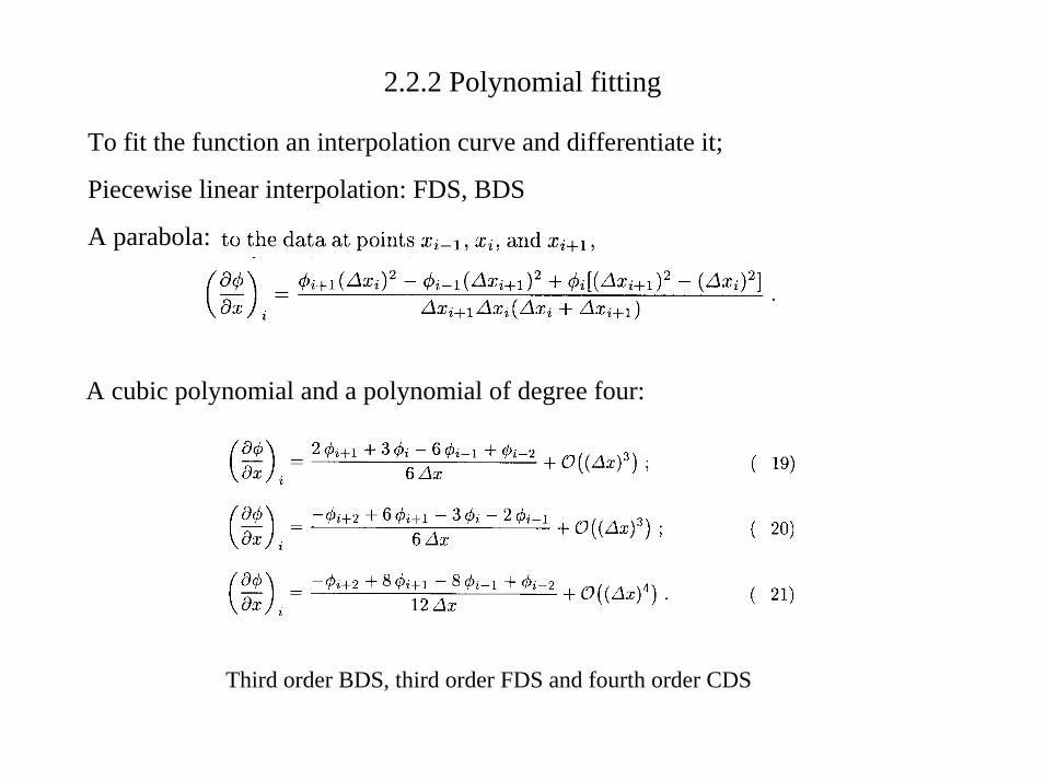
2.2.2 Polynomial fitting
To fit the function an interpolation curve and differentiate it;
Piecewise linear interpolation: FDS, BDS
A parabola:
A cubic polynomial and a polynomial of degree four:
Third order BDS, third order FDS and fourth order CDS

2.3 Approximation of the second derivativeApproximation from xi+1, xi

second derivative

2.4 Approximation of mixed derivatives
non-orthogonal coordinate systemcombining the 1D approximationsThe order of differentiation can be changed

2.5 Implementation of boundary conditions
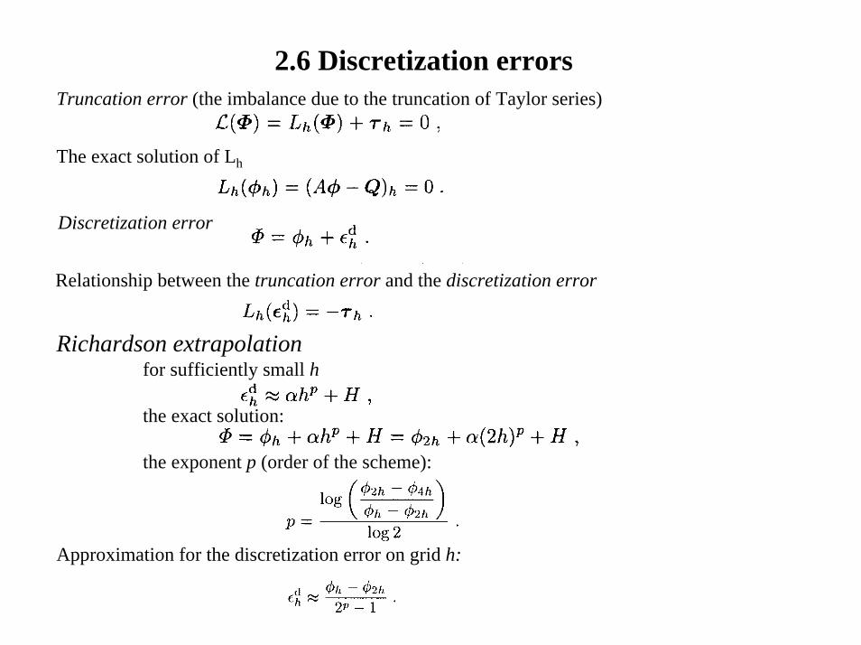
2.6 Discretization errorsTruncation error (the imbalance due to the truncation of Taylor series)
The exact solution of Lh
Discretization error
Relationship between the truncation error and the discretization error
Richardson extrapolationfor sufficiently small h
the exact solution:
the exponent p (order of the scheme):
Approximation for the discretization error on grid h:
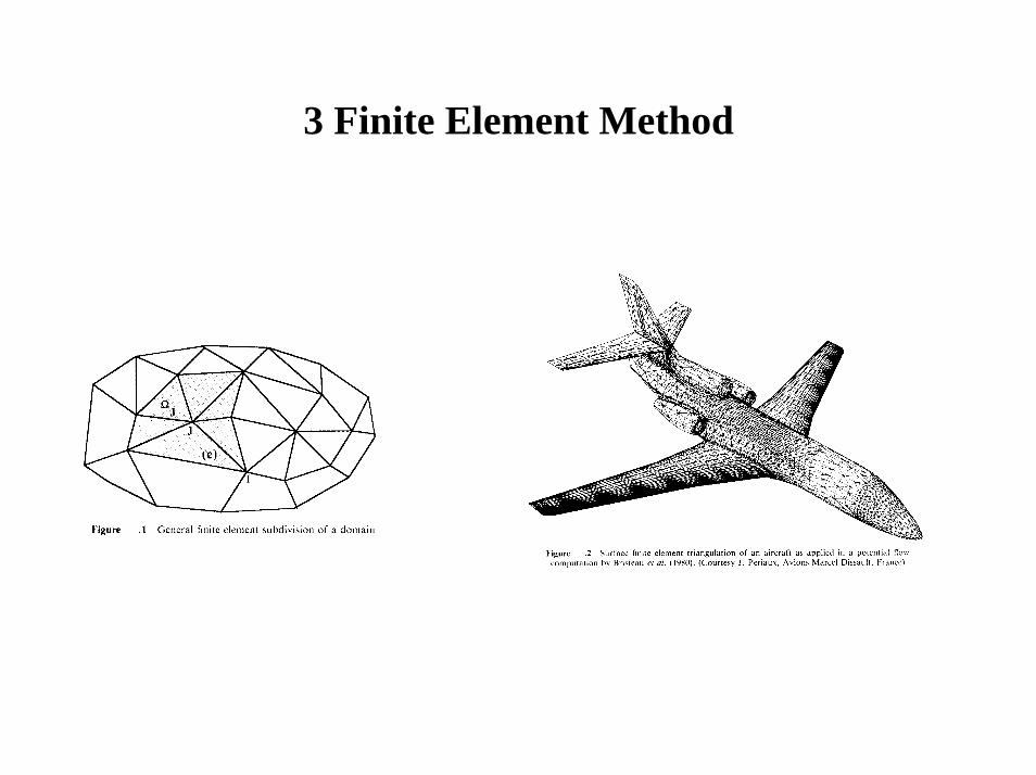
3 Finite Element Method

3.1 Interpolation function
Approximation by linear combinations of basis functions (shape, interpolation or trial functions)
Mehods based on defining the interpolation function on the whole domain:trigonometric functions: collocation and spectral methodsloccaly defined polynomials: standard finite element methods

One dimensional linear function

3.2 Method of weighted residuals

4 Finite Volume Method
• 4.1 Introduction

4.2 Approximation of surface integrals

4.3 Approximation of volume integrals

4.4 Interpolation practices

Linear interpolation

Quadratic Upwind Interpolation (QUICK)

Higher-order schemes
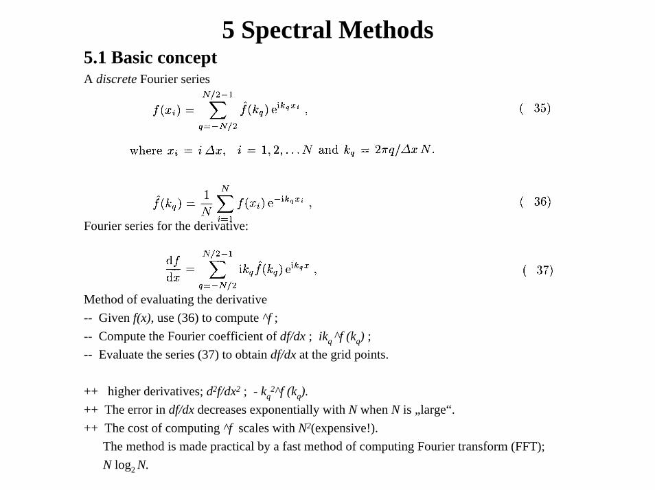
5 Spectral Methods5.1 Basic conceptA discrete Fourier series
Fourier series for the derivative:
Method of evaluating the derivative-- Given f(x), use (36) to compute ^f ;-- Compute the Fourier coefficient of df/dx ; ikq ^f (kq) ;-- Evaluate the series (37) to obtain df/dx at the grid points.
++ higher derivatives; d2f/dx2 ; - kq2^f (kq).
++ The error in df/dx decreases exponentially with N when N is „large“.++ The cost of computing ^f scales with N2(expensive!).
The method is made practical by a fast method of computing Fourier transform (FFT);N log2 N.

5.2 A Fourier Galerkin method for the wave equation

Example

Error

7 Time integration
Unsteady flows Initial value problem (Initial boundary value problem)
Steady flows Boundary value problem
Boundary condition
Boundary value problem
Steady solution
Solution at time t=t
time t=0Initial condition
t
t=0
Initial value problem

7.1 Methods for Ordinary Differential Equation (ODE)
Two-level methods

Two-level methods

Predictor-Corrector method
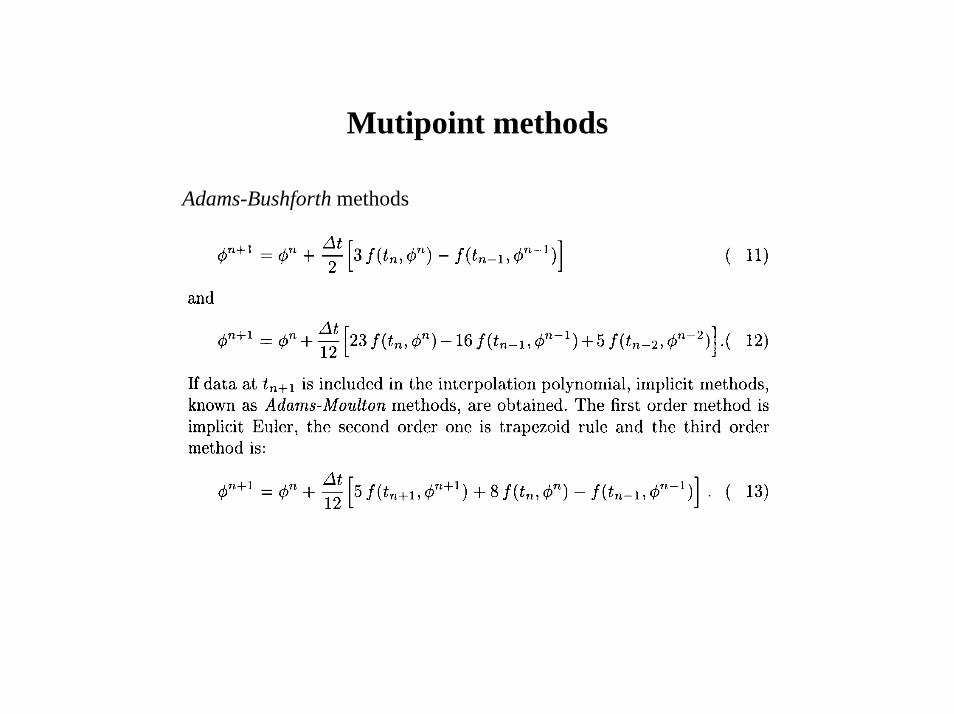
Mutipoint methods
Adams-Bushforth methods

Runge-Kutta methodsThe second order Runge-Kutta method
The fourth order Runge-Kutta method

Other methods
An implicit three-level second order scheme

8 Stability analysisOne dimensional convection equation
Finite difference equation; forward in time, centered in space

Q: Does a solution of FDE converges to the solution of PDE?
approximatePDE FDE
0
?Solution of PDE Solution of FDE
Ans.: „Even if we solve the FDE that approximate the PDE appropriately, the solution may not always be the correct approximation the exact solution of PDE.
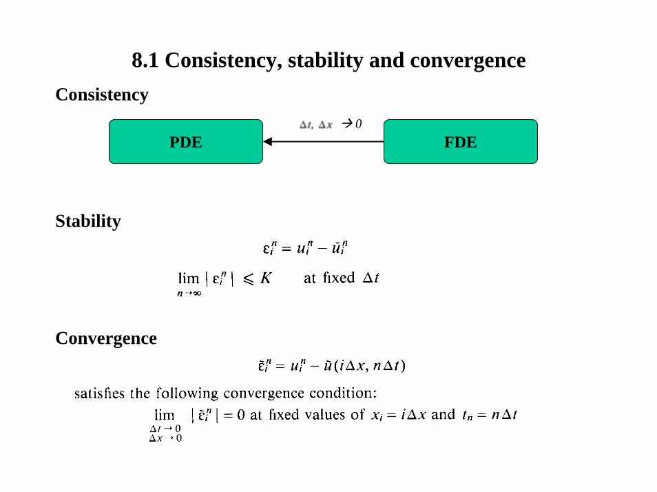
8.1 Consistency, stability and convergenceConsistency
0PDE FDE
Stability
Convergence

Lax‘s equivalence theorem
consistentPDE FDE
L : linear operator
Solution of PDE
stable0
Solution of FDE
convergent

Truncation error

8.2 Von Neumann‘s method
Fourier representation of the error on the grid points

FTCS method for 1D convection equation
Amplification factor G
Fourier series of the error
|G| > 1: Unconditionally unstable

Forward in time, forward in space(upwind scheme)
CFL (Courant Freedrichs, Levey) condition

BTCS method (Backward in time, centered in space)
|G| < 1: Unconditionally stable

Stability limit of 1D diffusion equation

8.3 Hirt‘s method

8.4 The matrix methodMatrix form
Spectral radius of the matrix C (maximum eigenvalue of C)

9 Iterative methods for algebraic systems

Linear equations : matrix form

9.0 Direct methods9.0.1 Gauß elimination
A = A21/A11
Forward eliminationupper triangular matrix
Back substitution
+ The number of operations (for large n) ~ n3 / 3 (n2 / 2 in back substitution) + pivoting (not sparse large systems)

9.0.2 LU decomposition
Solution ofAx = Q (0)
Factorization into lower (L) and upper (U) triangular matricesA = LU (1)
Into two stages:U x = y (2)L y = Q (3)

9.0.3 Tridiagonal matrixThomas algorithm / Tridiagonal Matrix Algorithm (TDMA)
+ the number of operations ~ n (cf n3 ,Gauß elimination)

Iterative methods : Basic concept
Matrix representation of the algebraic equationA u = Q (1)
After n iterations approximate solution u n , residual r n :r n = Q - A u n (2)
The convergence error:e n = u – u n (3)
Relation between the error and the residual:A e n = r n (4)
The purpose: to drive r n to zero. e n 0

Iterative procedureA u = Q
Iterative schemeM u n+1 = N u n + B (5)
Obvious property at convergence : u n+1 = u n
A = M – N, B = Q (6)
More generally,PA = M – N, B = PQ (7)
P : pre-conditioning matrixAn alternative to (5): -M u n
M (u n+1 – u n ) = B – (M –N) u n (8)or
M d n = r n
d n = u n+1 – u n : correction
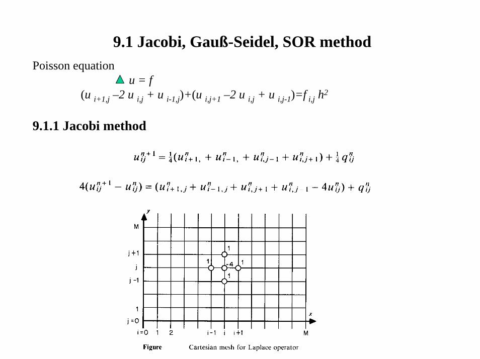
9.1 Jacobi, Gauß-Seidel, SOR methodPoisson equation
u = f(u i+1,j –2 u i,j + u i-1,j)+(u i,j+1 –2 u i,j + u i,j-1)=f i,j h2
9.1.1 Jacobi method

9.1.2 Gauß-Seidel method
9.1.3 SOR method

9.1.4 SLOR method
9.1.5 Red-Black SOR method

9.1.5 Zebra line SOR method

9.1.6 Incomplete LU decomposition : Stone’s method
Idea : an approximate LU factorization as the iteration matrix M
M = LU = A + N
Strongly implicit procedure (Stone)
N (non-zero elements on diagonals corresponding to all non-zero diag. of LU )N u ~ 0u*NW ~ a ( uW + uN – uP ), u*SE ~ a ( uS + uE – uP )a < 1

9.1.7 ADI methodElliptic problem parabolic problem
trapezoidal rule in time and CDS in space
at time step n+1
alternating direction implicit (ADI) method
splitting or approximate factorization methods
The last term ~ O((dt)3)

9.2 Conjugate Gradient (CG) methodNon-linear solvers Newton-like methods
global methods descent method
Minimization problem
A: positive definiteSteepest descentsConjugate gradient method
with p1 and p2 conjugate
condition number of A
preconditioningC-1AC-1Cp=C-1Q

9.3 Multi Grid method

Spectral view of errors

Fourier modes

Restriction

Interpolation

Coarse grid scheme
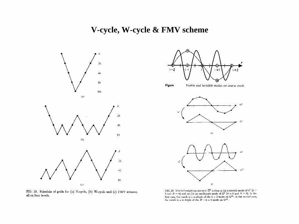
V-cycle, W-cycle & FMV scheme

9.4 Non-linear equations and their solution9.4.1 Newton‘s method
linearization
new estimate
x0
x1
y = f(x)y
o x

Newton‘s method
System of non-linear equations
Matrix of the system: the Jacobian
The system of equations
linearization

9.4.2 Other techniques
Picard iteration approach
Newton‘s method

9.5 Examples

Transonic flow over an airfoil

11 Incompressible Navier Stokes (NS) equations11.1.0 Incompressible fluid
Incompressible fluid flow Compressible fluid flowMa < 0.3 Ma > 0.3
density variation d� ~ Ma2
Mach number Ma = (v/c) v : velocity, c : sound speed
ex.Ma < 0.3
c air (101.3hPa, 300K) ~ 340 m/s, v < 100 m/s ( 360 km/h ),
c water ~ 1000 m/s, v < 300 m/s.

11.1.1 Dynamic similitude
Reynolds numberRe =
u : velocity scale, l : length scale, v : kinematic viscosityex.U = 10 m/s, L = 1 m, v = 0.15 St, Re ~ 105. U = 0.1 m/s, L = 100 m, Re ~ 105.
ρ
η ν
u l u l=

11.2 The pressure Poisson equation methodGoverning equations
Navier-Stokes equations
Explicit Euler method
Pressure Poisson equation

11.3 The projection methodA system of two component equations
The pressure P a projection function
The projection step (BTCS)
Poisson equation with the Neumann boundary condition :

11.4 Implicit Pressure-Correction methodDiscrete Poisson equation for the pressure : The momentum equations (implicit method)
Outer iteration (iterations within one time step): Pressure-correction
Modification of the pressure field The (tentative) velocity at node P
For convenience,
The discretized continuity equation
The (final) corrected velocities and pressure :
The relation between the velocity and pressure corrections :
Pressure-correction equation :
Common practice; neglect unknowns ~u‘SIMPLE algorithm
more gentle way

Implicit Pressure-Correction methodApproximate u‘ by a weighted mean of the neighbour values
Neglect ~u‘ in the first correction step. The second correction to the velocity u‘‘ :
The second pressure correction equation:Approximate ~u‘ by :
Approximate relation between u‘ and p‘ : Essentially an iterative method for pressure-correction equation with the last term treated explicitly;PISO algorithm
The coefficient in the pressure-correction equation A A + ... And the last term disappears.SIMPLEC algorithm
Pressure-correction with the last term neglected.p‘ correct the velocity field to obtain um
i.The new pressure field is calculated from pressure equation using ~ um
i instead of ~ um*i
SIMPLER algorithm (Patankar 1980)

Implicit Pressure-Correction methodThe SIMPLE algorithm does not converge rapidly due to the neglect of ~u‘ in the pressure-correction equation.It has been found by trial and error that convergence can be improved if :
SIMPLEC, SIMPLER and PISO do not need under-relaxation of the pressure-correction. An optimum relation between the under-relaxation factors for v and p :The velocities are corrected by
i.e., ~u‘ is neglected. By assuming that the final pressure correction is app‘ :
By making use of correction equation, expression for ap:
If we use the approximation used in SIMPLEC, the equation reduces to :
In the absence of any contribution from source terms, if a steady solution is sought, ap = 1 - av
which has been found nearly optimum and yields almost the same convergence rate as SIMPLEC method.

11.5 Other methods11.5.1 Streamfunction-vorticity methods
Stream function
Kinematic equation
Vorticity transport equation
-NS equations have been replaced by a set of two PDEs.-A problem : the boundary conditions, especially in complex geometries.
-The values of the streamfunction at boundaries.-Vorticity at the boundary is not known in advance.-Vorticity is singular at sharp corners.
11.5.2 Artificial compressibility methods
Artificial continuity equation
beta : an artificial compressibility parameterThe pseudo-sound speed:
should be much much faster than the vorticity spreads criterion on the lowest value of beta. Typical values are in the range between 0.1 and 10.Obviously,
should be small.

12 Some remarks on incompressible flows