Embed Size (px)
Citation preview

Working Paper 341
Conditional alphas and realized
betas
Valentina Corradi
Walter Distaso Marcelo Fernandes
CEQEF - Nº09
Working Paper Series 06 de dezembro de 2013

WORKING PAPER 341 – CEQEF Nº 09 • DEZEMBRO DE 2013 • 1
Os artigos dos Textos para Discussão da Escola de Economia de São Paulo da Fundação Getulio
Vargas são de inteira responsabilidade dos autores e não refletem necessariamente a opinião da
FGV-EESP. É permitida a reprodução total ou parcial dos artigos, desde que creditada a fonte.
Escola de Economia de São Paulo da Fundação Getulio Vargas FGV-EESP www.eesp.fgv.br

Conditional alphas and realized betas
Valentina Corradi
University of Surrey
Walter Distaso
Imperial College London
Marcelo Fernandes
Sao Paulo School of Economics, FGV
and Queen Mary University of London
This version: October 29, 2013
Abstract: This paper proposes a two-step procedure to back out the conditional alpha of a
given stock using high-frequency data. We first estimate the realized factor loadings of the stocks,
and then retrieve their conditional alphas by estimating the conditional expectation of their risk-
adjusted returns. We start with the underlying continuous-time stochastic process that governs
the dynamics of every stock price and then derive the conditions under which we may consistently
estimate the daily factor loadings and the resulting conditional alphas. We also contribute empiri-
cally to the conditional CAPM literature by examining the main drivers of the conditional alphas
of the S&P 100 index constituents from January 2001 to December 2008. In addition, to confirm
whether these conditional alphas indeed relate to pricing errors, we assess the performance of both
cross-sectional and time-series momentum strategies based on the conditional alpha estimates. The
findings are very promising in that these strategies not only seem to perform pretty well both in
absolute and relative terms, but also exhibit virtually no systematic exposure to the usual risk
factors (namely, market, size, value and momentum portfolios).
Keywords: asset pricing, conditional CAPM, pricing errors, realized beta, risk-adjusted performance.
Acknowledgments: We thank the valuable comments by Greg Connor, Andrew Karolyi, Asger Lunde, Hashem
Pesaran and Olivier Scaillet as well as by seminar participants at the Einaudi Institute for Economics and Finance,
Geneva Finance Research Institute, National University of Ireland Maymooth, Queen Mary, PUC-Rio, Rotterdam
Erasmus University, University of Birmingham, University of Lecce, University of Surrey, University of Vienna,
Nonlinear and Financial Econometrics Conference: A Tribute to A. Ronald Gallant (Toulouse, May 2011), CEF/MMF
Workshop on Empirical Finance: Some Recent Methodological Developments and Applications (London, May 2011),
Statistics and Modeling for Complex Data (Ecole des Ponts Paris-Tech, June 2011), Meeting of the Brazilian Finance
Society (Rio de Janeiro, July 2011), the Italian Congress on Econometrics and Empirical Economics (Genoa, January
2013), the Royal Statistical Society (Newcastle, September 2013), and the International Workshop in Financial
Econometrics (Natal, October 2013). We are also much indebted to Christian Brownlees for so generously providing
the realized beta data. The usual disclaimer applies.
1

1 Introduction
The unconditional CAPM does not provide a good description of equity markets. It fails to explain
important market anomalies, such as the size effect, the value premium and momentum. In addition,
the absence of pricing errors does not suffice to ensure a zero unconditional alpha because market
betas may change over time in tandem with market volatility and/or with risk premia. For instance,
allowing for time-varying betas helps explain most of the (unconditional) value premium given that
value stocks are riskiest precisely when risk premium is higher, namely, in recession times (Petkova
and Zhang, 2005; Zhang, 2005).
The usual fix is to assume a conditional CAPM framework in which alphas and betas are affine on
pre-determined predictor variables, e.g., stock characteristics, interest rates and spreads as well as
other business-cycle indicators.1 Ferson, Simin and Sarkissian (2008) discuss three stylized factors
that emerge from this literature. First, market betas do vary over time in a significant manner
(Shanken, 1990; Cochrane, 1996; Ferson and Schadt, 1996; Jagannathan and Wang, 1996; Ferson
and Harvey, 1999; Lettau and Ludvigson, 2001; Santos and Veronesi, 2006). Second, the intercept
of the conditional alpha term is smaller than the unconditional alpha. This means that conditional
asset pricing models entail on average smaller pricing errors than their unconditional versions.
Third, despite of their better fit, conditional asset pricing models still fail in view that conditional
alphas are not only nonzero, but also time-varying. See, among others, Christopherson, Ferson and
Glassman (1998), Wang (2002), Ang and Chen (2007), and Adrian and Franzoni (2009).
This paper goes after these pricing errors. We build on the realized beta technology (Barndorff-
Nielsen and Shephard, 2004; Andersen, Bollerslev, Diebold and Wu, 2006) to come up with a novel
two-step procedure to estimate conditional alphas. In the first stage, we employ high-frequency
data to retrieve a stock’s realized beta or, in general, any other risk factor loading. The second step
then backs out the conditional alpha by estimating the conditional expectation of the risk-adjusted
return (i.e., the return in excess over the realized risk premia) at a lower frequency. The resulting
estimator is nonparametric, enjoying much more flexibility and robustness than the usual paramet-
ric estimators. In particular, it does not require conditional alphas and betas to depend linearly on
1 Note however that, if the conditional betas are affine, the conditional alpha is necessarily quadratic in theabsence of arbitrage opportunities (Gagliardini, Ossola and Scaillet, 2013).
2
the conditioning state variables, reducing misspecification risks in a substantial manner. Although
we focus on the conditional CAPM in the empirical analysis, the framework is general enough
to handle any asset pricing model with tradeable factors. The conditional CAPM with higher-
order moments ensues as one includes additional powers of the S&P 500 index returns, whereas
adding exchange-traded funds (ETFs) based on size and book-to-market considerations would boil
down to a conditional Fama-French model. Alternatively, we could also think of continuous and
discontinuous market betas as in Todorov and Bollerslev (2010).
Integrating observations at different sampling frequencies is now new to finance. Merton (1980)
notes that one can accurately estimate the variance over a fixed interval of time by summing squared
returns at a sufficiently high sampling frequency. French, Schwert and Stambaugh (1987) and
Ghysels, Santa Clara and Valkanov (2005) accordingly exploit daily (squared) returns to estimate
the monthly volatility in their search for the risk-return tradeoff, whereas the realized measure
literature employs intraday returns to compute daily realized variances, covariances, and market
betas (Barndorff-Nielsen and Shephard, 2004; Andersen et al., 2006; Ait-Sahalia and Mykland, 2009;
Andersen, Bollerslev and Diebold, 2009; Ait-Sahalia, Fan and Xiu, 2011) as well as to conduct
statistical inference for parametric continuous-time stochastic volatility models (Bollerslev and
Zhou, 2002; Corradi and Distaso, 2006; Todorov, 2009). More recently, Chang, Kim and Park
(2009) combine low- and high-frequency observations to estimate continuous-time factor pricing
models with constant factor loadings.
Traditionally, the focus is on testing for the absence of systematic pricing errors as in Gibbons,
Ross and Shanken (1989). More recently, Grundy and Martin (2001), Lewellen and Nagel (2006),
Li and Yang (2011) and Ang and Kristensen (2012) consider more general settings for testing
conditional asset pricing models with time-varying alphas and betas. They advocate for the use of
daily data to estimate monthly factor loadings within short local windows. We take this idea to the
limit by employing ultra-high frequency data to estimate daily betas, but then change the focus
from assessing the magnitude of pricing errors to how could we take advantage of them. This is in
line with Hansen and Richard’s (1987) and Wheatley’s (1989) point that it is impossible to test a
conditional factor pricing model without observing the investors’ information sets. In addition, we
also differ from previous nonparametric approaches by assuming that both alphas and betas are
3

measurable functions of conditioning state variables and hence predictable. This allows us to carry
out a more-than-descriptive analysis of pricing errors. Apart from looking at the main features of
the time-varying alphas (e.g., persistence), we can also ask all sort of interesting questions about
alpha portability and about the cross-sectional variation in the partial effect of each instrument.
Along these lines, we examine the main forces driving the pricing errors in the S&P 100 index
constituents from January 2001 to December 2008. We first estimate the daily market betas using a
multivariate realized kernel with refresh time as in Barndorff-Nielsen, Hansen, Lunde and Shephard
(2011), so as to account for market microstructure noise and nonsynchronicity issues. The realized
betas consistently estimate the daily conditional betas as long as the latter are constant within a
day. Accordingly, we assume a continuous-time process for the stock prices in which the drift and
diffusive parameters are measurable functions of conditioning state variables that evolve only at
the daily frequency. This ensures that the conditional alphas and betas vary over time on a daily
basis, but remain constant at any higher (intraday) frequency.
Given the realized market betas, we next compute risk-adjusted returns by subtracting the real-
ized risk premia. By definition, the latter is the sum of the conditional alpha and the idiosyncratic
innovation. The key to identify the pricing errors is that the conditional expectation of the idiosyn-
cratic term is zero. We thus estimate the conditional expectation of the risk-adjusted returns using
a nonparametric approach, so as to minimize misspecification and overconditioning risks (Boguth,
Carlson, Fisher and Simutin, 2011). Differently from Welch and Goyal (2008), we work at the daily
frequency, ruling out many of the usual suspects for the conditioning state variables. Accordingly,
we employ as lagged predictors various interest rates and spreads, market liquidity and volatility
measures as well as characteristic-based portfolios based on momentum, short- and long-term rever-
sals, size, and value effects. By conditioning on firm-specific attributes, we take the view of Graham
and Dodd (1934), Lakonishok, Shleifer and Vishny (1994), Haugen and Baker (1996), and Daniel
and Titman (1997) that these variables are perhaps useful to spot systematic mispricings in equity
markets. And, by taking all possible candidates available at the daily frequency as instruments, we
also reduce the risk of underconditioning (Ghysels, 1998; Harvey, 2001).
We are also particularly attentive to data snooping and spurious regression biases that may
affect the estimation of conditional alphas (Ferson et al., 2008). Due to their local nature, kernel
4

estimators are relatively less prone to the spurious regression problem that may arise in the presence
of persistent regressors. We also control to some extent for data snooping by considering only
a few principal components of the various instruments we entertain. Further, conditioning on
principal components also helps reduce the dimensionality of the nonparametric regression without
having to assume from the start that the conditional alphas are nonconstant as other dimension
reduction techniques would require (see, among others, Li, 1991; Ichimura, 1993; Huang, Horowitz
and Wei, 2010). It does not seem fair after all to presuppose nonzero conditional alphas if the aim
is to uncover them.
Given the conditional alpha estimates, the next step is to assess whether it is profitable to trade
them away. We first show that the nonparametric alpha estimates convey information about future
stock returns as one would expect if they indeed relate to pricing errors. We then implement simple
self-financed trading strategies that take long positions in stocks with positive conditional alphas,
while shorting stocks with negative conditional alphas. We determine whether a given conditional
alpha is large/low enough to justify a long/short position by conditioning either on cross-sectional
or time-series quantiles. This gives way to cross-sectional and time-series momentum strategies
based on conditional alphas rather than on raw returns as in Jegadeesh and Titman (1993) and
Moskowitz, Ooi and Pedersen (2012), respectively. Due to the time variation in the alphas, we
would have in principle to rebalance our long-short portfolio every day, raising the issue of alpha
portability after transaction fees. We thus entertain different holding horizons so as to effectively
reduce the portfolio turnover of the trading strategies.
We find that the cross-sectional and time-series momentum strategies based on nonparametric
alphas easily outperform not only the S&P 500 index, but also the equal-weight portfolio of the
S&P 100 index constituents, even after controlling for transaction costs. In particular, the best
performances are from the alpha-based cross-section strategy with a holding period of 3 days and
the time-series strategies with holding periods of 10 and 22 days. The same does not apply, however,
to similar strategies based on affine alphas. There is a striking difference in performance once one
move from affine to nonparametric alphas. Finally, one may wonder whether it is possible to achieve
a comparable performance by means of simpler passive trading strategies. A traditional multifactor
analysis reveals that the answer is negative. Although they entail positive unconditional alphas,
5

the alpha-based strategies display very little exposure to the market, size, value and momentum
risk factors. This is very reassuring given our conditional CAPM assumption.
The rest of this paper is as follows. Section 2 spells out the assumptions we make on the
continuous-time multivariate process that governs the dynamics of stock prices. Note that we do
not start from the continuous-time version of the CAPM as in Mykland and Zhang (2006), for
otherwise the CAPM would not hold in discrete time (Longstaff, 1989). Section 3 develops the
asymptotic justification of the conditional alpha estimator, controlling for the fact that we only
observe the realized beta and not the true conditional beta. Section 4 examines whether there
are pricing errors in the S&P 100 index constituents and whether it is profitable to trade them
away. Section 5 offers some concluding remarks. Appendix A collects all technical proofs for the
realized beta estimator, whereas Appendix B outlines the extension to the multivariate realized
kernel estimator that accounts for both nonsynchronicity and market microstructure noise.
2 Conditional factor pricing model
This section proposes a consistent two-step procedure to identify and estimate conditional alphas.
We first estimate daily conditional betas using a realized beta approach that takes advantage of
intraday observations. This yields consistent estimates of the conditional betas as long as the
sampling interval shrinks to zero (i.e., infill asymptotics). We then carry out a nonparametric
regression of the resulting daily risk-adjusted returns on conditioning state variables to estimate
daily pricing errors. Asymptotic validity of this second step relies in turn on a long-span asymptotic
theory, that is to say, on a large enough number of trading days. Given the interplay between infill
and long-span asymptotics, we must pay special attention not only to the underlying continuous-
time process, but also to the rates at which the number of intraday observations and the number
of days in the sample go to infinity.
In the following, we derive a discrete-time conditional multifactor asset pricing model from the
exact discretization of a conditional semimartingale process in continuous time. This is important
because we must ensure that the probability limit of the realized betas is indeed the vector of factor
loadings in the discrete-time multifactor model. Our discretization results complement well those
in Longstaff (1989) and Chang et al. (2009). The former shows that temporally aggregating the
6
continuous-time CAPM results in a multifactor model in discrete time, whereas the latter considers
a continuous-time model that is also consistent with a discrete-time multifactor model. The main
difference is that our setting delivers conditional alphas and betas that evolve in discrete time.
2.1 From continuous to discrete time
Let Pi(s) and F (s) respectively denote the log-prices at time s of the i-th asset (i = 1, . . . , N)
and of kF portfolios mimicking the common risk factors that drive assets’ excess returns. For
instance, the CAPM considers the market portfolio as a single factor (kF = 1), whereas Fama and
French (1992) advocate for a three-factor model that controls for size and book-to-market effects
(kF = 3). We assume that both Pi(s) and F (s) follow continuous-time diffusion processes, with
drift and volatility parameters evolving in discrete time as measurable functions of kC conditioning
instruments Ct. One may think of the latter either as state variables that reflect changes in the
future investment opportunity set as in Merton’s (1973) ICAPM. In particular, all predetermined
instruments that help predict future discounted returns are natural candidates. More precisely, for
any t ≤ s < t+ 1 and i ∈ 1, . . . , N,
dPi(s) = µi,t ds+ Σ′i,t dW F (s) + σi,t dWi(s) (1)
dF (s) = µF,t ds+ ΣF,t dW F (s), (2)
where µi,t ≡ µi(Ct) and µF,t ≡ µF (Ct) are drift parameters, Σi,t ≡ Σi(Ct) is a kF × 1 vector that
determines the exposure of asset i to each risk factor, ΣF,t ≡ ΣF (Ct) is the kF × kF covariance
matrix of the common risk factors, WF (s) is a kF−dimensional standard Brownian motion, and
Wi(s) is a standard Brownian motion independent of WF (s). We next document under which
conditions asset and factor prices are continuous-time semimartingale processes. This is crucial
because semimartingale prices are not only consistent with no-arbitrage considerations, but also
necessary in the infill asymptotic theory we use to justify the realized beta measures.
Lemma 1: Let Xi(s) = (Pi(s),F (s)) evolve as in (1) and (2). Let also C(s) = Ct for any
s ∈ [t, t+ 1) and define the filtration FC(s) = σ(C(τ), τ ≤ s) for s > 0. If C(s) is independent of
both Wi(s) and WF (s), then Xi(s) is a conditional semimartingale with independent increments
given FC(s).
7

The assumption that C(s) is independent of Wi(s) and WF (s) implies that E[Σ′i,tWi(s)
]= 0
and that E [ΣF,tWF (s)] = 0. This does not imply however that F (s) and C(s) are independent.
In fact, the common risk factors F (s) depend on the conditioning state variables Ct for any
s ∈ [t, t + 1) through the drift and diffusion parameters. In addition, it follows from Lemma 1
that, given the value of Ct, the continuous-time process Xi(s) has independent increments for any
s ∈ [t, t+1). This means that market microstructure effects are responsible for any autocorrelation
pattern within the interval [t, t + 1), say, a day. In contrast, due to the dependence on Ct, daily
increments xi,t =∫ t+1t dXi(s) may display genuine autocorrelation.
Suppose that we have M equidistant observations within a day starting at time t, namely,
Pi,t+`/M and F t+`/M with j = 0, . . . ,M − 1. We then define the vector of realized betas as
βi,t,M =
[M−1∑`=0
(F t+ `+1M− F t+ `
M)(F t+ `+1
M− F t+ `
M)′
]−1 M−1∑`=0
(F t+ `+1M− F t+ `
M)(Pi,t+ `+1
M− Pi,t+ `
M). (3)
Barndorff-Nielsen and Shephard (2004) show that, under very mild regularity conditions, for all t,
plimM→∞
βi,t,M = Σ−1FF,t ΣF,t Σi,t ≡ βi,t, (4)
where ΣFF,t = ΣF,tΣ′F,t. Note also that the conditioning state variables Ct are the only drivers of
the daily factor loadings in that βi,t ≡ βi(Ct), and hence betas are constant within a day. This
is much milder than Lewellen and Nagel’s (2006) assumption of constant monthly/quarterly betas.
In addition, it also ensures that realized betas converge to conditional betas without any need for
further conditioning.
For simplicity, we henceforth assume without loss of generality that F t+j/M consists of or-
thogonal risk factors, so that ΣFF,t is diagonal.2 Further note that the estimator in (3) assumes
that we observe prices and factors without measurement error. However, there is ample evidence
that market microstructure noise is present in high-frequency transaction data. As a remedy, one
should employ a realized beta estimator that is robust to such a contamination. This is the route
we take in the empirical part, using of Barndorff-Nielsen et al.’s (2011) multivariate realized kernel
approach. For notational simplicity, we relegate the case of microstructure noise robust estimators
to Appendix B.
2 In fact, we can always make the factors orthogonal via a rotation matrix Bt such that F t+`/M = BtF t+`/M
and F′t+`/M βi,t,M = F ′t+`/M βi,t,M , where βi,t,M denote the realized betas associated with the orthogonal factors.
8

We now move to discrete time by letting ri,t+1 ≡∫ t+1t dPi(s) and f t+1 ≡
∫ t+1t dF (s) denote
continuously-compounded returns over the time interval [t, t+ 1). It then follows from (1) and (2)
that
ri,t+1 = µi,t + σi,t
∫ t+1
tdWi(s) + Σ′i,t
∫ t+1
tdWF (s) (5)
f t+1 = µF,t + ΣF,t
∫ t+1
tdWF (s), t = 1, . . . , T. (6)
This means that
(ri,t+1,f t+1
)|Ct ∼ N
((µi,t
µF,t
),
(σ2i,t + Σ′i,t Σi,t Σ′i,t ΣF,t
ΣF,t Σi,t ΣFF,t
)),
and so further conditioning on factor returns entails
ri,t+1|(f t+1,Ct) ∼ N(µi,t + (f t+1 − µF,t)′Σ−1
FF,tΣF,t Σi,t, σ2i,t + Σ′i,tΣi,t −Σ′i,tΣ
−1FF,tΣi,t
).
Using the definition of the betas in (4) then yields the following discrete-time factor model
ri,t+1 = αi,t + f ′t+1βi,t + εi,t+1, (7)
with αi,t = µi,t − µ′F,tβi,t and εi,t+1|(f t+1,Ct) ∼ N(
0, σ2i,t + Σ′i,tΣi,t −Σ′i,tΣ
−1FF,tΣi,t
).
It is now easy to appreciate why we assume that the drift and diffusive parameters in (1) and
(2) evolve in discrete time. If the conditioning state variables were evolving in continuous time, (5)
and (6) would then represent just a discrete-time approximation. As a result, the probability limit
of the realized betas would differ from the true integrated beta given by the integral of the ratio:
plimM→∞
βi,t,M =
(∫ t+1
tΣFF,s ds
)−1 ∫ t+1
tΣF,sΣi,s ds.
It is worth stressing however that this will only hurt our identification strategy if the discrete-time
approximation is such that E (εi,t+1|Ct) differs from zero.
2.2 Retrieving conditional alphas from realized betas
Let Zi,t+1 ≡ ri,t+1 − f ′t+1βi,t denote the daily risk-adjusted return at time t + 1. It then follows
from (7) that Zi,t+1 = αi,t + εi,t+1. Identification of the conditional alpha stems from the facts
that the conditional expectation of εi,t+1 is zero and that αi,t is measurable in the information set.
Altogether, this means that αi,t ≡ E(Zi,t+1|Ct) and hence it would suffice to estimate the condi-
tional expectation of the risk-adjusted returns to back out the conditional alphas. Unfortunately,
9

this is infeasible because we do not directly observe the conditional betas and so the risk-adjusted
returns.
To obtain a feasible estimator, we proceed in two steps. First, we adjust asset returns for risk
using a realized beta approach, namely,
Zi,t+1,M = ri,t+1 − f ′t+1βi,t,M = ri,t+1 − f ′t+1βi,t − f ′t+1
(βi,t,M − βi,t
)= αi,t + εi,t+1 − f ′t+1
(βi,t,M − βi,t
)= Zi,t+1 − f ′t+1
(βi,t,M − βi,t
).
Second, we estimate the conditional expectation E(Zi,t+1,M |Ct) of the realized risk-adjusted returns
using nonparametric kernel methods. In the next section, we establish under mild conditions that
the difference between the feasible and infeasible estimators shrinks to zero as the number of
intraday observations M increases.
The fact that we employ a nonparametric regression is in stark contrast with the usual practice
of imposing an affine structure for the conditional alpha. The motivation is not only to capture
nonlinear effects in a more efficient manner, but also to alleviate any spurious regression issue that
may arise from the use of persistent, though still weak dependent, conditioning instruments (Ferson
et al., 2008). In particular, Robinson (1986) shows that the local nature of kernel regressions breaks
some of the persistence of mixing regressors for large enough bandwidths. The price we pay for more
robust alpha estimates comes in the guise of the curse of dimensionality. Typically, the dimension
of the vector Ct is relatively high so as to avoid underconditioning bias. However, nonparametric
rates of convergence decrease with the dimensionality of the conditioning state vector. We thus
condition the realized risk-adjusted returns on the k largest principal components of Ct (rather
than on the full vector).3 This allows us to consider a large number of conditioning state variables
without incurring into the usual data mining biases that arise in the search for predictor variables
(Ferson et al., 2008).
Let then PCt = (PC1,t, . . . , PCk,t)′ denote the k < kC principal components of Ct, where kC is
the dimension of Ct. In the sequel, we assume that E(εi,t+1|PCt) = 0 for all i and, with a slightly
3 This is obviously a suboptimal dimension-reduction technique given that it boils down to a particular case of themultiple index model in which we take the linear combinations as given by the principal component analysis (Park,Sriram and Yin, 2010). Indeed, there are several more efficient methods for dimension reduction in a nonparametricsetting: e.g., sliced inverse regression (Li, 1991) and group-Lasso-type criteria (Huang et al., 2010). However, iden-tification of these estimators require a nonconstant conditional expectation. While we conjecture that alpha is notconstant for most stocks, it does not seem fair to rule out constant or even zero alphas beforehand.
10

abuse of notation, we define αi,t = E(Zi,t+1|PCt). While the condition E(εi,t+1|Ct) = 0 does not
necessarily imply E(εi,t+1|PCt) = 0, their difference will nevertheless shrink to zero as k → kC .
This means that, if we condition on enough principal components to capture most of the variation
in Zi,t+1, E(εi,t+1|PCt) will get very close to zero. The idea of summarizing the predictive content
of many variables into few principal components is exactly what explains the popularity of factor
augmented predictive models (see, e.g., Bai and Ng, 2006).
The conditional alpha estimator then is
αi,t = mi,T,M (PCt) =
1ThkT
∑T−1`=1 Zi,`+1,MK
(PC`−PCt
hT
)gT (PCt)
, (8)
where gT (PCt) = 1ThkT
∑T−1`=1 K
(PC`−PCt
hT
)is the kernel estimator of the density g of the vector of
principal components. Note that we must establish a uniform result over the support of the principal
components because they are stochastic processes. To circumvent the difficulty of estimatingmi(pc)
over regions of low density, we consider a trimmed version of mi,T,M (pc) as in Andrews (1995):
trT mi,T,M (pc) = mi,T,M (c) 1c ∈ GT (pc)
, (9)
where GT (pc) = c : gT (pc) > dT . Section 3 establishes the uniform consistency of mi,T,M (PCt)
by showing that(∫Rk|trT (mi,T,M (pc))−mi(pc)|Q g(pc) dpc
) 1Q
= op(1) (10)
for some Q > 0 as dT → 0 at an appropriate rate.
Apart from the conditional alpha, we also consider Treynor and Black’s (1973) appraisal ratio:
Ai,t = Ai(Ct) =E(Zi,t+1|Ct)√Var(Zi,t+1|Ct)
=αi,t√
E(ε2i,t+1|Ct),
where εi,t = Zi,t−αi,t. By comparing the conditional alpha to the conditional idiosyncratic volatility,
it gauges the extra units of unsystematic risk investors have to bear for deviating from a passive
management strategy. We estimate the conditional appraisal ratio by means of
Ai,t,M = Ai,T,M (PCt) =mi,T,M (PCt)√
m(2)i,T,M (PCt)− m2
i,T,M (PCt), (11)
where mi,T,M (PCt) is given by (8) and
m(2)i,T,M (PCt) =
1ThkT
∑T−1`=1 Z
2i,`+1,MK
(PC`−PCt
h
)gT (PCt)
.
11

The advantage of using appraisal ratios instead of alphas to pick individual stocks is that it puts
some discipline on the portfolio selection process by focusing on the magnitude of the mispricing
relative to the noise level.
3 Asymptotic Theory
In this section, we derive the consistency of the nonparametric estimators we propose for the
conditional alpha and appraisal ratio. We first establish the asymptotic consistency of the infeasible
estimator based on unobservable risk-adjusted returns:
αi,t+1 = mi,T (PCt) =
1ThkT
∑T−1`=1 Zi,`+1K
(PC`−PCt
hT
)gT (PCt)
and then show that proxying for the latter by the realized risk-adjusted returns has no asymptotic
cost. For the consistency of the conditional alpha estimator, we require the following conditions to
hold.
Assumption A
(i) For i = 1, . . . , N , µi,t, σi,t, and the elements of Σi,t, µF,t and ΣF,t in (1) and (2) are
FC(t)−measurable and δ−dominated, with δ > 2.4
(ii) For i = 1, . . . , N , E |Zi,t|δ <∞ with the same δ > 2 as in (i), and Zi,t+1,CtT−1t=1 is strictly
stationary and α−mixing with coefficients αj such that∑∞
j=1 α1−2/δj <∞.
(iii) The distribution of Ct with respect to the Lebesgue measure on RkC is absolutely continuous,
with a bounded density φ that is twice continuously differentiable with bounded derivatives.
(iv) The multivariate kernel functionK is a k-dimensional product kernel with marginal bounded
density K, such that∫R xK(x) dx = 0 and
∫R x
2K(x) dx < ∞. In addition, the univariate
kernel K has an absolutely integrable characteristic function Ψ(u) =∫R exp(iux)K(x) dx such
that∫R |Ψ(u)| du <∞.
(v) Let mi(pc) = E(Zi,t+1|PCt = pc) for i = 1, . . . , N . The product mi(pc) g(pc) is bounded
and twice continuously differentiable on Rk with bounded derivatives for i = 1, . . . , N .
4 Recall that Xt is δ−dominated if |Xt| ≤ Dt for some Dt such that E(Dδt ) <∞.
12

(vi) suppc∈Rk |mi(pc)| <∞ for i = 1, . . . , N and∫Rk g(pc)1−a dpc <∞ for some 0 < a < 1.
Assumptions A(ii) − (iii) relate to the conditioning state variables Ct rather than to their
first k principal components as the statistic in (10). Because each principal component is a linear
combination of the kC <∞ elements of Ct, it follows straightforwardly that PCt is also α−mixing,
with the same mixing size as Ct. This means that A(ii) also holds for PCt. The marginal density
of each individual principal component is absolutely continuous because they all result from the
direct convolution of the kC absolutely continuous marginals of the conditioning instruments. As
principal components are mutually orthogonal, their joint density is absolutely continuous on Rk.
Assumption A(iii) thus ensures that PCt has a absolutely continuous density on Rk. Assumption
A(iv) is standard, holding for instance for the multivariate standard normal kernel we use in the
empirical application. Assumptions A(v) − (vi) regulate the smoothness and the boundedness of
the regression function as well as the thickness of the tails of the regressors. For example, if g(pc)
is multivariate normal,∫Rk g(pc)1−a dpc <∞ holds for any a arbitrarily close to 1.
We now ready to document our first result that there is no asymptotic difference between the
feasible and infeasible estimators.
Proposition 1: Let the conditions of Lemma 1 as well as Assumption A hold. If T,M, h−1T →∞
and d−1T
(M−1h−kT +M−1/2T−1/2h−kT
)→ 0, then trT mi,T (pc)−trT mi,T,M (pc) is of order op(1)
uniformly in pc ∈ GT (pc).
It is immediate to see that we allow M to grow at a slower rate than T . This is empirically
very important. In addition, the conditions on the rate of growth of M are much weaker than in
Corradi, Distaso and Swanson’s (2009) Theorem 1. This happens because the estimation error in
the betas affects only the dependent variable of the nonparametric regression, and hence it does
not enter in the kernel function.
Proposition 2: Let the conditions of Lemma 1 as well as Assumption A hold. It then follows for
a as in Assumption A(vi) and 0 < Q <∞ that[∫Rk|trT (mi,T,M (pc))−mi(pc)|Q g(pc) dpc
] 1Q
= Op(T−1/2M−1/2h−kT +M−kh−kT ) +O(h2
Td−2T )
+ Op(d−2T T−1/2h−kT ) +Op(d
a/QT ).
13

In the sequel, we establish the consistency of the appraisal ratio estimator. To this end, we
have to strengthen Assumption A so as to deal with the second moment of the risk-adjusted return,
namely, on m(2)i (pc) = E(Z2
i,t+1|PCt = pc).
Assumption B
(i) For i = 1, . . . , N , E |Zi,t|2δ < ∞ with δ > 2 and Zi,t+1,CtT−1t=1 is strictly stationary and
α−mixing with coefficients αj such that∑∞
j=1 αβ−2β
j <∞.
(ii) For i = 1, . . . , N , m(2)i (pc) g(pc) is bounded and twice continuously differentiable on Rk and
with bounded derivatives.
(iii) For i = 1, . . . , N and for some 0 < a < 1, suppc∈Rk∣∣∣m(2)
i (pc)∣∣∣ <∞ and
∫Rk g(pc)1−a dpc <∞.
Define trT
(Ai,T,M (pc)
)= Ai,T,M (pc) 1
pc ∈ GT (pc)
. The next result ascertains the consis-
tency of the trimmed nonparametric estimator of the appraisal ratio.
Proposition 3: Let the conditions of Lemma 1 as well as Assumptions A and B hold. It then
follows for 0 < Q <∞ that(∫Rk
∣∣∣trT (Ai,T,M (pc))−Ai(pc)
∣∣∣Q g(pc) dc
) 1Q
= Op(T−1/2M−1/2h−kT +M−kh−kT )
+ Op(T−1/2h−kT d−2
T ) +O(h2Td−2T ) +Op(d
a/QT ),
with a as in Assumption B(iii).
In the next section, we assess the performance of our estimators using real equity data. The idea
is that, if our conditional alpha estimates are indeed uncovering pricing errors, they should predict
to some extent future stock returns. To this end, we proceed in four steps. First, we compute
daily factor loadings for the S&P 100 index constituents. Second, we estimate their conditional
alphas and appraisal ratios by conditioning the corresponding risk-adjusted returns on a number
of instruments. Third, we form portfolios that take long positions on undervalued stocks and short
positions on overvalued stocks. Finally, we assess their performances to examine the economic
relevance of the conditional alpha estimates.
14

4 Mispricing in the S&P 100 index constituents
To estimate the daily factor loadings, we must first define the risk factors we will consider. We
employ a single-factor model using the S&P 500 index as proxy for the market portfolio. The
main advantage is the ease of interpretation given that the conditional CAPM is a well-established
model. In addition, it is much easier to find intraday data for a proxy of the market portfolio than
for some of the other risk factors in the literature. We thus employ tick-by-tick data for the S&P
500 index as well as for each of the S&P 100 index constituents to estimate daily realized market
betas. The sample period runs from 2 January 2001 to 30 December 2008, amounting to 1,915
trading days. We exploit as much as possible the richness of the tick-by-tick information by using
a realized kernel approach with refreshing time. The latter is very convenient because it is robust
to market microstructure noise as well as to nonsynchronous trading (see Appendix B for details).
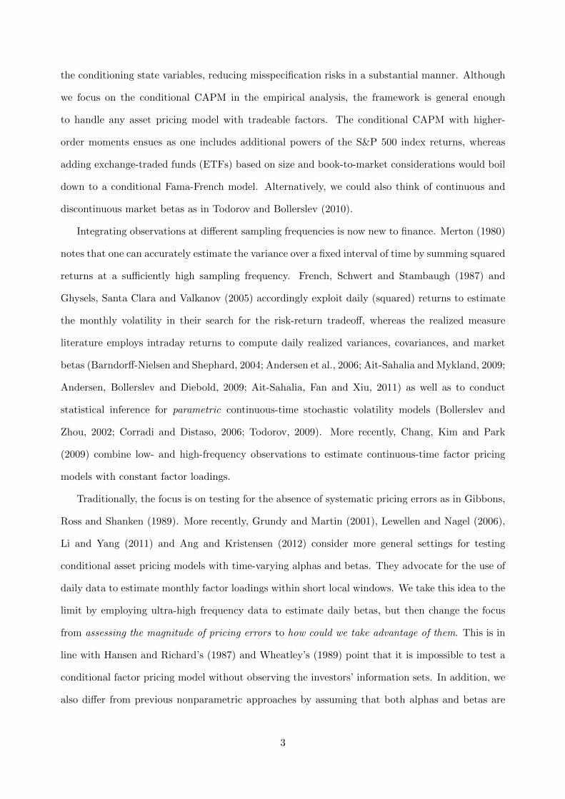
Figure 1 displays the time series behavior of the cross-sectional quantiles of the daily betas
we estimate. Cross-sectional dispersion seems fairly constant over time, even if the median beta
increases significantly throughout 2002. There is also some evidence of co-movement among betas,
with the first three principal components explaining over a third of the overall variation.
We next compute daily risk-adjusted returns for each stock in the sample. To obtain the pricing
errors, we estimate the conditional expectation of the risk-adjusted returns using a kernel regression
approach. In particular, we employ a multivariate standard Gaussian kernel with rule-of-thumb
bandwidths. As for the amount of trimming in (9), uniform consistency requires dT = O(hkζT ) with
0 < ζ < 1/4. Note that, because hT → 0 as T → ∞, trimming becomes more aggressive as ζ
declines. We set ζ to 0.20 in order to enforce only a mild trimming, though we also experiment
with other values of ζ in Section 5.3. The daily frequency of the realized betas dictates the choice
of the instruments, ruling out most macroeconomic variables as well as the predictors that Welch
and Goyal (2008) use for the risk premium. In particular, we proxy the state variables using the
following instruments: the changes in the VIX index and in the Fed Fund rate, the volatility risk
premium (namely, difference between the VIX index and realized volatility), size and value factors,
short- and long-term reversal factors, the credit and term spreads, and the momentum factor.
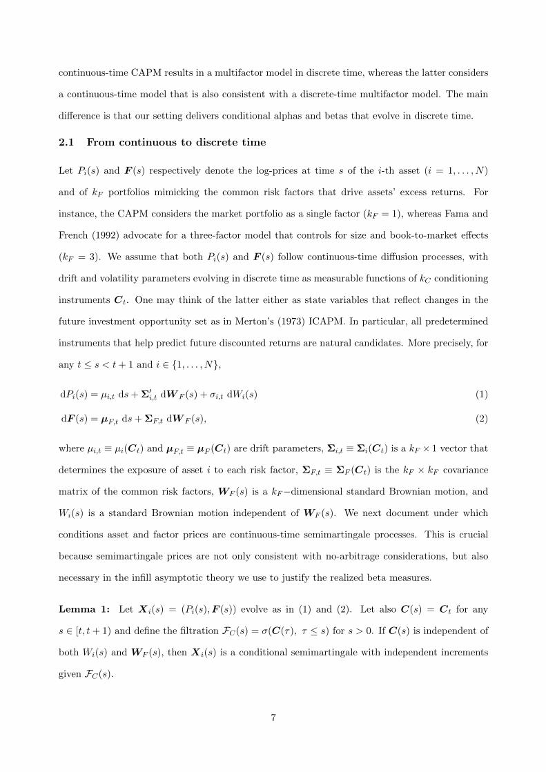
Figure 2 displays the time series behavior of the cross-sectional quantiles of the daily pricing
errors. In contrast to the pattern we observe for the realized market betas, the cross-sectional dis-
15
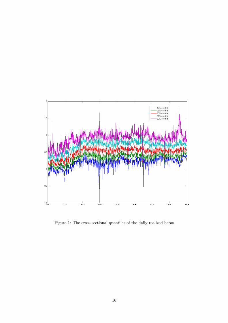
Figure 1: The cross-sectional quantiles of the daily realized betas
16
persion of the conditional alpha estimates is much more erratic, exhibiting a great deal of volatility
clustering. In particular, cross-sectional dispersion is relatively much higher in the beginning and in
the end of the sample period. Finally, there is also some moderate evidence of co-movement among
alphas, with the first three principal components explaining over 45% of the overall variation. A
similar picture arises if one considers affine alphas as opposed to nonparametric alphas. The only
significant difference is that affine alphas co-move much more strongly, with the first three principal
components responding for over 87% of the total variation.
Figure 2: The cross-sectional quantiles of the nonparametric alpha estimates
Interestingly, daily realized betas feature a lot of persistence, displaying to some extent long
range dependence. Figure 3(a) shows a slow decay in the average autocorrelation function, definitely
slower than exponential. In contrast, Figure 3 shows that the average autocorrelation functions are
quite low for both affine and nonparametric alpha estimates, especially for the latter.
(a) realized beta (b) affine alpha (c) nonparametric alpha
Figure 3: Average autocorrelation function of the daily realized betas and alpha estimates
17
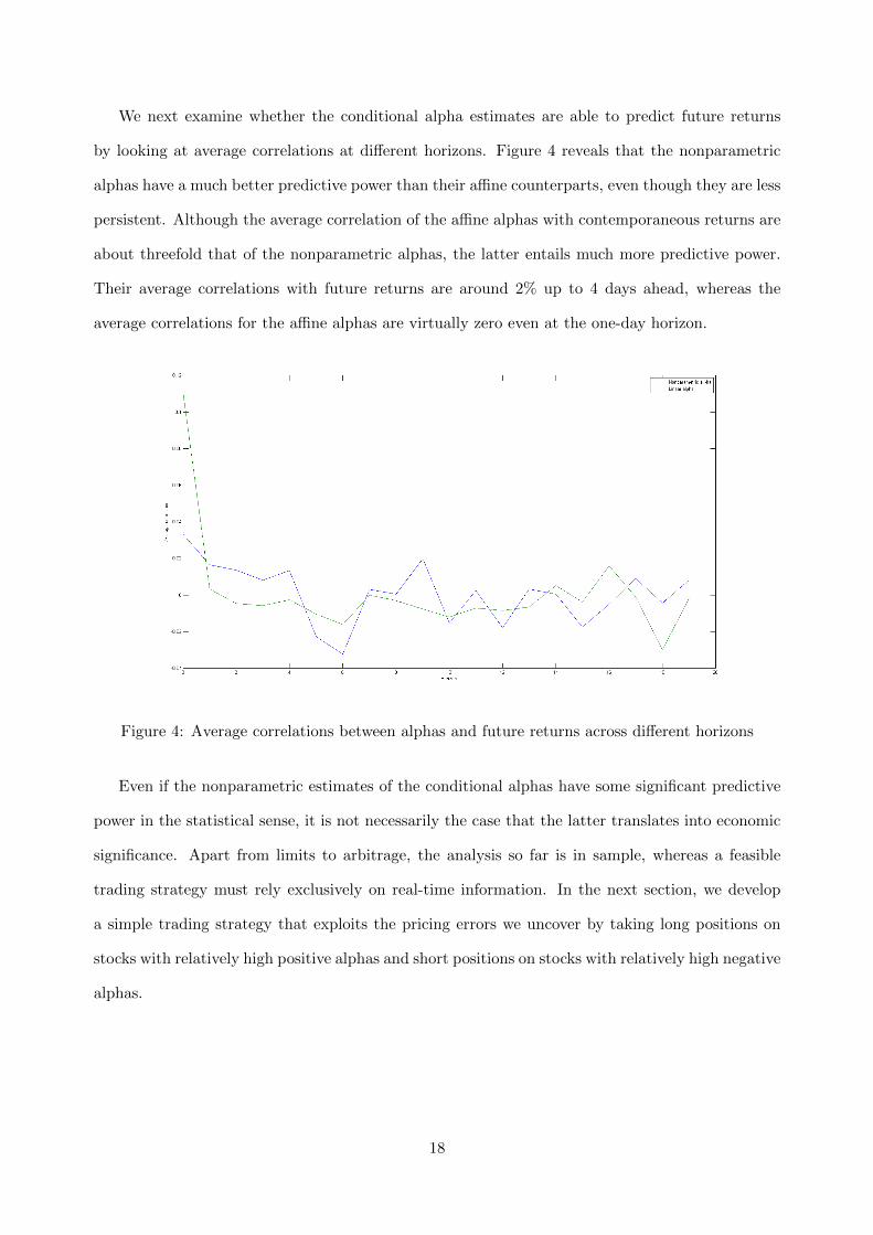
We next examine whether the conditional alpha estimates are able to predict future returns
by looking at average correlations at different horizons. Figure 4 reveals that the nonparametric
alphas have a much better predictive power than their affine counterparts, even though they are less
persistent. Although the average correlation of the affine alphas with contemporaneous returns are
about threefold that of the nonparametric alphas, the latter entails much more predictive power.
Their average correlations with future returns are around 2% up to 4 days ahead, whereas the
average correlations for the affine alphas are virtually zero even at the one-day horizon.
Figure 4: Average correlations between alphas and future returns across different horizons
Even if the nonparametric estimates of the conditional alphas have some significant predictive
power in the statistical sense, it is not necessarily the case that the latter translates into economic
significance. Apart from limits to arbitrage, the analysis so far is in sample, whereas a feasible
trading strategy must rely exclusively on real-time information. In the next section, we develop
a simple trading strategy that exploits the pricing errors we uncover by taking long positions on
stocks with relatively high positive alphas and short positions on stocks with relatively high negative
alphas.
18

5 Is it profitable to trade these pricing errors away?
If the conditional alpha estimates indeed correspond to pricing errors, we should be able to arbitrage
them away. To this end, we may exploit either the cross-section or the time series information in
the alphas. We start with the former by sorting stocks cross-sectionally according to alphas. We
then take long positions on stocks within some upper quantile and short stocks within some lower
quantile. This is similar in spirit to Jegadeesh and Titman’s (1993) momentum strategy. There
are two key differences, though. First, the signal is given by the alpha estimates rather than past
raw returns. Second, we assume a much shorter holding period given the preliminary correlation
analysis in Figure 4.
Alternatively, we may compare conditional alphas to their time-series quantiles. This would
yield a sort of alpha-based counterpart to Moskowitz et al.’s (2012) time-series momentum strategy.
In particular, we long any stock with alpha currently at some top quantile of the historic distribution
and short any stock with alpha currently at some bottom quantile. Given that we observe some
persistence in the nonparametric alphas, we expect the time-series momentum strategy to perform
better than the cross-sectional for longer holding periods.
To ensure feasibility in practice, we form these long-short portfolios based on real-time estimates.
To this effect, we estimate the pricing errors using an expanding window with an initial subsample of
375 daily observations. This means that the precision of the conditional alpha estimates increases
over time as the sample size grows. In addition, we also consider the corresponding long-short
strategies based on appraisal ratios. Finally, we contemplate variations of the alpha-based strategies
in which we correct the alpha estimates by means of a risk-free rate adjustment.
5.1 Exploiting the cross-sectional information
In this section, we first describe in details the alpha-based strategies based on cross-sectional quan-
tiles and then report their performance. The trading algorithm is very simple. We first nonpara-
metrically estimate the daily conditional alphas of each stock using past data. We then daily sort
the stocks by the value of their alphas so as to compute daily cross-sectional quintiles. We next
form a long-short portfolio by purchasing the top quintile stocks and selling the bottom quintile
stocks. We keep the portfolio for a given holding period, varying from 1 to 5 days, and then liqui-
19

date the position. To assess performance in a realistic fashion, we impose a transaction cost of 4
basis points to each trade. This is slightly conservative given that the S&P 100 index constituents
are all actively traded large caps. Note also that, to ensure feasibility in practice, we employ only
historic information in the estimation of the conditional alphas. In particular, we use an expanding
window and hence the precision of the alpha estimates increases over time as the sample size grows.
Table 1 reports the main descriptive statistics. In line with the correlation analysis, the returns
on the long-short cross-sectional momentum strategy seem to increase with the holding period
until 3 days and then start declining. The same applies to the Sharpe ratio, which achieves its
maximum of 0.90 at the 3-day holding period, even if the volatility of the strategy is monotonically
increasing with the holding period. As expected, the long-short nature of the portfolio helps reduce
the volatility of the strategy in a substantial manner. Individually, the long and short portfolios
are much more volatile than the resulting long-short combination. Interestingly, the long-short
strategy displays significant positive skewness for holding periods of up to 3 days, mostly due to
the short positions on stocks with negative alpha.
Adjusting for the risk-free rate does not change qualitatively the big picture. Recall that we
back out the conditional alphas from the daily risk-adjusted returns Zi,t+1 ≡ ri,t+1 − βi,t ft+1,
where ft denotes the returns on the S&P 500 index. Note that the returns are not in excess over
the risk-free rate and hence, to obtain risk-adjusted excess returns, we would have to compute
Zi,t+1 ≡ ri,t+1 − rf,t+1 − βi,t (ft+1 − rf,t+1) = ri,t+1 − βi,t ft+1 − (1− βi,t) rf,t+1
= Zi,t+1 − (1− βi,t) rf,t+1,
where rf,t+1 is the return on a risk-free investment from time t to t+1. The conditional expectation
of the risk-adjusted excess returns is then equal to the unadjusted conditional alpha minus a pre-
determined correction term that depends both on the risk-free rate and on the market beta. We
thus adjust our conditional alpha estimates for the risk-free rate by subtracting (1− βi,t,M )rf,t+1,
where βi,t,M is the realized market beta. To proxy for the risk-free rate rf,t+1, we employ the
1-month Treasury bill rate available at Kenneth French’s website.5
Because we are mostly interesting in the cross-sectional alpha quantiles (rather than on levels),
the risk-free rate does not matter as much as the realized market beta given that only the latter
5 See http://mba.tuck.dartmouth.edu/pages/faculty/ken.french/data_library.html.
20

Figure 5: Cumulative returns to the cross-sectional momentum strategy with a 3-day holding period
does vary across stocks. However, the risk-adjusted return already reflects, even if only partially,
the information on the market beta and hence it is not surprising that the qualitative results do
not change if we focus on the risk-adjusted excess returns instead. Table 3 indeed reveals that the
only difference the risk-free adjustment makes is that the realized returns become slightly lower.
As expected from Figure 4, putting together a long-short portfolio based on affine alphas (as
opposed to nonparametric) does not yield as promising results. Tables 2 and 4) show a slight
improvement in performance only for a holding period of one day, with nonparametric alphas
clearly dominate otherwise. In particular, the cross-sectional momentum strategies based on an
affine specification for the conditional alpha display higher volatility than their nonparametric
counterparts.
To gauge the informational content in the conditional alphas, we next examine the performance
of the cross-sectional momentum strategy relative to the S&P 100 index and to the equal-weight
portfolio of all index constituents. Figure 5 plots the cumulative returns to the cross-sectional
momentum strategy with a holding period of 3 days. It reveals the conditional alphas help select
stocks with better future performance. The wedge between the cumulative returns of the long
portfolio of the cross-sectional strategy and those of the equal-weight portfolio is indeed sizeable.
The same pattern arises for different holding periods as well as for other variants of the strategy
21

(e.g., with or without risk-free adjustment).
5.2 A time-series momentum strategy based on conditional alphas
We next engineer a trading strategy that exploits the time series properties of conditional alpha
estimates. The motivation is to take benefit of the persistence of the nonparametric alphas by
looking at the quantiles of the historical distribution of the alphas. So, what matters now is not
whether a given stock currently has a very large alpha relative to the other stocks. We gauge the
relevance of the pricing error relative to its past magnitudes. In particular, we go long in any stock
whose alpha is currently at the top 25% of its historical distribution, and short any stock with alpha
at the bottom quartile. Given that we expect more persistence in the time-series quantiles than
in the cross-sectional quantiles, we now also contemplate longer holding periods before liquidating
the position. We thus present results for holding periods of 1, 5, 10 and 22 days. Finally, we apply
the same 4 basis points fee to each transaction.
Table 7 reports the main results. Both realized returns and volatility of the time-series strategy
seem to increase with the holding period. The long-short strategies that rebalance their portfolios
every 10 and 22 days achieve annualized average returns of 37% and 59%, with Sharpe ratios of 0.82
and 0.92, respectively. It is interesting to notice that skewness is once again always positive, whereas
kurtosis decreases with the holding period. In general, the time-series momentum strategy based
on conditional alphas entails higher returns than the cross-sectional strategy, probably because it
captures some degree of persistence.
Differently from the cross-sectional strategy, correcting the conditional alpha estimates by the
risk-free rate ameliorates the performance of the time-series momentum portfolio, essentially be-
cause it helps reduce the volatility of the strategy. As we are now looking at the quantiles of the
historic distribution, the risk-free rate starts to matter as well as the dynamics of the realized
market betas. Accordingly, the risk-free adjustment has a much higher impact than if we were
restricting our attention to the cross-section of the pricing errors.
It is not surprising that the time-series momentum strategy yields a poorer performance if based
on affine alphas given the lack of persistence in the latter. Tables 8 and 10 also reveal that the long
portfolio of the strategy entails particularly low returns across all holding periods. In addition, as
in the cross-sectional case, trading affine conditional alphas brings about much more volatility than
22
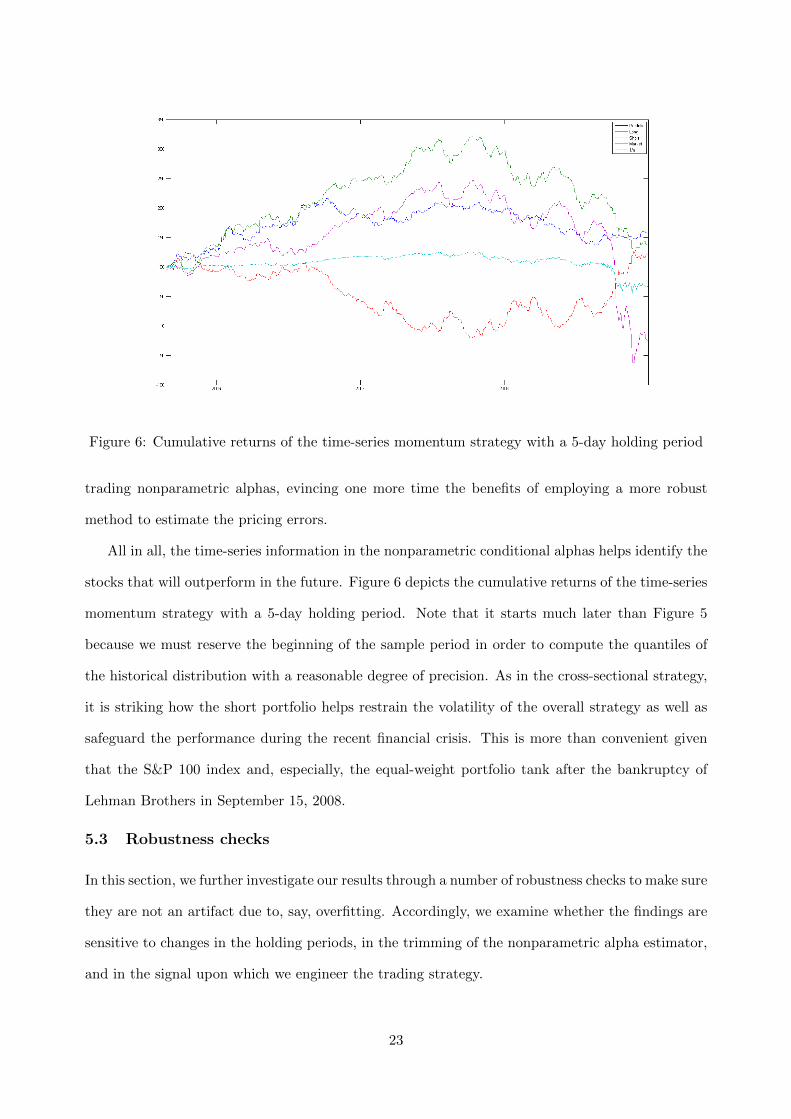
Figure 6: Cumulative returns of the time-series momentum strategy with a 5-day holding period
trading nonparametric alphas, evincing one more time the benefits of employing a more robust
method to estimate the pricing errors.
All in all, the time-series information in the nonparametric conditional alphas helps identify the
stocks that will outperform in the future. Figure 6 depicts the cumulative returns of the time-series
momentum strategy with a 5-day holding period. Note that it starts much later than Figure 5
because we must reserve the beginning of the sample period in order to compute the quantiles of
the historical distribution with a reasonable degree of precision. As in the cross-sectional strategy,
it is striking how the short portfolio helps restrain the volatility of the overall strategy as well as
safeguard the performance during the recent financial crisis. This is more than convenient given
that the S&P 100 index and, especially, the equal-weight portfolio tank after the bankruptcy of
Lehman Brothers in September 15, 2008.
5.3 Robustness checks
In this section, we further investigate our results through a number of robustness checks to make sure
they are not an artifact due to, say, overfitting. Accordingly, we examine whether the findings are
sensitive to changes in the holding periods, in the trimming of the nonparametric alpha estimator,
and in the signal upon which we engineer the trading strategy.
23

We start with the holding period. In the absence of transaction costs, one could well rebalance
the portfolio every day to fully exploit the daily changes in the conditional alphas. However,
as soon as transaction costs are present, rebalancing too much would imply excessive turnover.
This raises a tradeoff between shortening the holding period to trade current (rather than past)
pricing errors and lengthening the holding period to mitigate transaction costs. Our choice of the
holding periods to report for the cross-sectional and time-series momentum strategies follows from
the preliminary correlation analysis between current and past alphas, and future returns. It is
nonetheless important to stress that the trends we observe in the performance analyses remain
valid for different holding periods.
As for the amount of trimming, it turns out that the performances of both cross-sectional and
time-series momentum strategies hardly change if we implement a more aggressive trimming scheme
(namely, ζ = 0.01, 0.10). However, they worsen a bit if we employ no trimming in the nonparamet-
ric estimation of the conditional alphas. This happens because sometimes the conditional alpha
estimates are large only because of a very low value of the denominator in (8). This is exactly the
sort of situation that trimming avoids, for it sets the alpha to zero if there is too much uncertainty
(i.e., very low density of the conditioning instruments). Accordingly, trimming puts some discipline
in the conditional alpha estimates, improving the performance of the alpha-based strategies.
Alternatively, we may account for the uncertainty in the estimation of the conditional alphas
by using appraisal ratios as a signal for the trading strategy. The appraisal ratio standardize the
alpha by the level of idiosyncratic volatility as in (11. This means assigning more weight to large
positive alphas in periods of low uncertainty. Tables 5 and 6 respectively report the results for
the cross-sectional momentum strategies based on the nonparametric and affine appraisal ratios,
whereas Tables 11 and 12 document the performance of their time-series counterparts.
We uncover some interesting evidence. Building a cross-sectional strategy on the basis of the
appraisal ratios reduces both returns and volatility, with a net effect of a lower Sharpe ratio. Using
affine appraisal ratios nonetheless seems to improve the short end of the strategy. Conversely,
for the time-series momentum strategies, the reduction in the volatility is substantial enough to
compensate the decline in the realized returns. In other words, the net effect is that Sharpe ratios
do increase. In contrast to what happens with the nonparametric alphas, the absence of trimming
24

does not affect much the strategies based on appraisal ratios for they already control to some extent
for the uncertainty in the nonparametric estimation.
5.4 Multifactor analysis
Although the cross-sectional and time-series momentum strategies based on conditional alpha esti-
mates perform well at first glance, it remains to show that it cannot be easily reproduced following
a passive strategy, such as traditional momentum. In what follows, we check whether they have
significant exposure to the usual risk factors, namely, the market, size, value and momentum factors
also available at Kenneth French’s website. To take into account the likely temporal dependence
among daily returns due to overlapping trading periods for multiple days holding periods, we use
Newey-West standard errors to compute robust t-ratios.
Tables 1 to 6 show in their Panel A that the cross-sectional momentum strategies yield positive
unconditional alphas (i.e., intercepts of the multifactor regression). This does not mean much
given that the risk factors are not tradeable and hence do not consider transaction costs (Berk and
van Binsbergen, 2011)see, for instance, the excellent discussion in. In addition, these intercepts
are significant only for the nonparametric approach and not always. The affine specification for
the pricing errors are never significant, on the other hand. More importantly, the cross-sectional
momentum strategy does not load on the Fama-French portfolios, with the exception perhaps to
the positive market beta of the alpha-based strategy that corrects for the risk-free rate.
The story is not so simple for the momentum factor. This is not surprising given that our
strategies are momentum-based, even if we do not sort the stocks by raw returns. The cross-
sectional strategies based on affine specifications have always a significantly positive loading on
the momentum portfolio, whereas the evidence is much milder for the nonparametric alphas and
appraisal ratios. It is also worth stressing that the risk factors do not explain more than a tiny
portion of the variation of the realized returns on the cross-sectional strategies.
Tables 7 to 12) reveal a few negative alphas, especially for short holding periods (reflecting
transaction costs) and for affine signals. As the time-series momentum strategies exhibit much
higher volatility, it is not surprising that the intercepts of the multifactor regression are insignificant.
The same largely applies to the three Fama-French factors as well. Interestingly, the loadings on
the momentum factor is markedly different from the previous case. The sign is not always positive
25

and, most importantly, there are not many significant coefficient estimates. Accordingly, the fit of
the multifactor models is even poorer than before.
All in all, the findings of the above multifactor analysis confirm the dominance of the trading
strategies rooted in the nonparametric conditional alphas (as long as we employ some trimming).
In particular, the stars are the cross-sectional strategy with a holding period of 3 days and the
time-series momentum strategy with a holding period of 22 days. The former entails the highest
annualized unconditional alpha as well as the highest appraisal, Sharpe and Sortino ratios among the
cross-sectional strategies (0.90, 22.40, and 0.86, respectively). The only significant factor loading is
for the momentum portfolio, with a coefficient of 0.15. The latter yields a striking annualized alpha
of 60.93 (though insignificant), with a Sharpe ratio of 0.92, Sortino ratio of 21.75, and appraisal
ratio of 0.80. In addition, it does not load on any of the usual risk factors in a significant manner.
6 Conclusion
This paper shows how to identify pricing errors within a multifactor asset pricing model. The
procedure is in two steps. We first estimate the conditional factor loadings (e.g., the market beta in
a conditional CAPM world) so as to control for the amount of risk. Once we risk-adjust the returns,
we then regress them on the state variables to back out the conditional alpha or pricing error.
Despite the simplicity of our two-stage estimator, it requires thinking very carefully about the joint
dynamics of factors and stock prices. In particular, we start with a multivariate diffusion process
in continuous time for which exact discretization yields the conditional multifactor asset pricing
model of interest. To accomplish this, we must assume that the drift and diffusive parameters are
measurable functions of state variables that change only in discrete time. Accordingly, the factor
loadings are also constant over shorter periods of time and hence we may estimate them using
high-frequency data by means of a realized approach. We provide conditions under which the error
we make in the realized estimation of the factor loadings does not affect the consistency of the
nonparametric regression we do to retrieve the conditional alpha.
To assess empirical relevance, we estimate daily conditional alphas for the S&P 100 index con-
stituents within a conditional CAPM world. To proxy for state variables, we employ as instruments
size, value, momentum and reversal mimicking portfolios as well as some interest-rate spreads and
26
market volatility measures. Although the resulting conditional alpha estimates exhibit little persis-
tence (even if they oscillate around zero), we nonetheless find that they correlate with future stock
returns in a significant manner. We thus check how exploiting the information in the conditional
alpha estimates would fair in practice. All in all, we find that momentum-type strategies based
on the conditional alpha estimates perform pretty well. Returns are indeed very high as well as
Sharpe and Sortino ratios, even if volatility is also high.
Interestingly, a traditional multifactor analysis reveals positive unconditional alphas as well
as very little exposure to the market, size, value and momentum risk factors. The latter is a
key result in that, if the true model were a conditional multifactor pricing model (rather than a
conditional CAPM), our conditional alpha estimates would then capture the exposure to the risk
factors other than the market portfolio. The fact that our alpha-based momentum strategies do not
have significant exposure to size, value and momentum effects seems to attest that the conditional
CAPM assumption is not so restrictive after all.
References
Adrian, T., Franzoni, F., 2009, Learning about beta: Time-varying factor loadings, expected re-
turns, and the conditional CAPM, Journal of Empirical Finance 16, 537–556.
Ait-Sahalia, Y., Fan, J., Xiu, D., 2011, High frequency covariance estimates with noisy and asyn-
chronous financial data, Journal of the American Statistical Association 105, 15041517.
Ait-Sahalia, Y., Mykland, P., 2009, Estimating volatility in the presence of market microstructure
noise: A review of the theory and practical considerations, in: Thomas Mikosch et al. (ed.),
Handbook of Financial Time Series, Springer-Verlag.
Andersen, T. G., Bollerslev, T., Diebold, F. X., 2009, Parametric and non-parametric volatil-
ity measurements, in: Lars P. Hansen and Yacine Ait-Sahalia (ed.), Handbook of Financial
Econometrics, North Holland, New York.
Andersen, T. G., Bollerslev, T., Diebold, F. X., Wu, G., 2006, Realized beta: Persistence and
predictability, in: T. Fomby and D. Terrell (ed.), Advances in Econometrics: Econometric
Analysis of Economic and Financial Time Series in Honor of R. F. Engle, and C. W. J.
Granger, Part B, Vol. 20, Elsevier, New York, pp. 1–39.
Andrews, D. W. K., 1995, Nonparametric kernel estimation for semiparametric models, Economet-
ric Theory 11, 560–596.
27

Ang, A., Chen, J., 2007, CAPM over the long run: 1926–2001, Journal of Empirical Finance
14, 1–40.
Ang, A., Kristensen, D., 2012, Testing conditional factor models, Journal of Financial Economics
106, 132–156.
Bai, J., Ng, S., 2006, Confidence intervals for diffusion index forecast and inference with factor-
augmented regressions, Econometrica 74, 1133–1155.
Barndorff-Nielsen, O. E., Hansen, P. H., Lunde, A., Shephard, N., 2011, Multivariate realised
kernels: Consistent positive semi-definite estimators of the covariation of equity prices with
noise and non-synchronous trading, Journal of Econometrics 162, 149–169.
Barndorff-Nielsen, O. E., Shephard, N., 2004, Econometric analysis of realized covariation: High
frequency based covariance, regression and correlation in financial economics, Econometrica
72, 885–925.
Berk, J. B., van Binsbergen, J. H., 2011, Measuring skill in the mutual fund industry, working
paper, Stanford University and NBER.
Boguth, O., Carlson, M., Fisher, A., Simutin, M., 2011, Conditional risk and performance evalua-
tion: Volatility timing, overconditioning, and new estimates of momentum alphas, Journal of
Financial Economics 102, 363–389.
Bollerslev, T., Zhou, H., 2002, Estimating stochastic volatility diusions using conditional moments
of integrated volatility, Journal of Econometrics 109, 33–65.
Chang, Y., Kim, H., Park, J. Y., 2009, Evaluating factor pricing models using high frequency panels,
working paper, Indiana University, Texas A&M University and Sungkyunkwan University.
Christopherson, J. A., Ferson, W. E., Glassman, D., 1998, Conditioning manager alpha on economic
information: Another look at the persistence of performance, Review of Financial Studies
11, 111–142.
Cochrane, J. H., 1996, A cross-sectional test of an investment-based asset pricing model, Journal
of Political Economy 104, 572–621.
Corradi, V., Distaso, W., 2006, Semiparametric comparison of stochastic volatility models using
realized measures, Review of Economic Studies 73, 635–667.
Corradi, V., Distaso, W., Swanson, N. R., 2009, Predictive density estimators for daily volatility
based on realized measures, Journal of Econometrics 150, 119–138.
28

Daniel, K., Titman, S., 1997, Evidence on the characteristics of cross sectional variation in stock
returns, Journal of Finance 52, 1–33.
Fama, E. F., French, K. R., 1992, The cross-section of expected stock returns, Journal of Finance
47, 427–465.
Ferson, W. E., Harvey, C. R., 1999, Conditioning variables and the cross-section of stock returns,
Journal of Finance 54, 1325–1360.
Ferson, W. E., Schadt, R., 1996, Measuring fund strategy and performance in changing economic
conditions, Journal of Finance 51, 425–462.
Ferson, W. E., Simin, T., Sarkissian, S., 2008, Asset pricing models with conditional alphas and
betas: The effects of data snooping and spurious regression, Journal of Financial and Quanti-
tative Analysis 43, 331–354.
French, K. R., Schwert, W., Stambaugh, R. F., 1987, Expected stock returns and volatility, Journal
of Financial Economics 19, 3–29.
Gagliardini, P., Ossola, E., Scaillet, O., 2013, Time-varying risk premium in large cross-sectional
equity datasets, working paper, University of Lugano, University of Geneva, and Swiss Finance
Institute.
Ghysels, E., 1998, On stable factor structures in the pricing of risk: Do time-varying betas help or
hurt?, Journal of Finance 53, 549–573.
Ghysels, E., Santa Clara, P., Valkanov, R., 2005, There is a risk-return tradeoff after all, Journal
of Financial Economics 76, 509–548.
Gibbons, M. R., Ross, S. A., Shanken, J., 1989, A test of the efficiency of a given portfolio,
Econometrica 57, 1121–1152.
Graham, B., Dodd, D., 1934, Security Analysis, McGraw-Hill, New York.
Grundy, B. D., Martin, J. S., 2001, Understanding the nature and risks and the source of the
rewards to momentum profits, Review of Financial Studies 14, 2978.
Hansen, L. P., Richard, S. F., 1987, The role of conditioning information in deducing testable
restrictions implied by dynamic asset pricing models, Econometrica 55, 587–614.
Harris, F. H. d., McInish, T. H., Shoesmith, G. L., Wood, R. A., 1995, Cointegration, error
correction and price discovery on informationally-linked security markets, Journal of Financial
and Quantitative Analysis 30, 563–581.
29
Harvey, C. R., 2001, The specification of conditional expectations, Journal of Empirical Finance
8, 573–637.
Haugen, R. A., Baker, N. L., 1996, Commonality in the determinants of expected stock returns,
Journal of Financial Economics 41, 401–440.
Huang, J., Horowitz, J. L., Wei, F., 2010, Variable selection in nonparametric additive models,
Annals of Statistics 38, 2282–2313.
Ichimura, H., 1993, Semiparametric least squares (sls) and weighted sls estimation of single-index
models, Journal of Econometrics 58, 71–120.
Jacod, J., 1997, On continuous conditional Gaussian martingales and stable converge in law, Sem-
inaire de Probabilites XXXI, Vol. 1635, Springer Verlag, New York.
Jagannathan, R., Wang, W., 1996, The conditional CAPM and the cross-section of stock returns,
Journal of Finance 51, 3–53.
Jegadeesh, N., Titman, S., 1993, Returns to buying winners and selling losers: Implications for
stock market efficiency, Journal of Finance 48, 65–91.
Lakonishok, J., Shleifer, A., Vishny, R. W., 1994, Contrarian investment, extrapolation and risk,
Journal of Finance 49, 1541–1578.
Lettau, M., Ludvigson, S., 2001, Consumption, aggregate wealth and expected stock returns, Jour-
nal of Finance 56, 815–849.
Lewellen, J., Nagel, S., 2006, The conditional CAPM does not explain asset pricing anomalies,
Journal of Financial Economics 82, 289–314.
Li, K. C., 1991, Sliced inverse regression for dimension reduction, Journal of the American Statistical
Association 86, 316–327.
Li, Y., Yang, L., 2011, Testing conditional factor models: A nonparametric approach, Journal of
Empirical Finance 18, 972–992.
Longstaff, F. A., 1989, Temporal aggregation and the continuous-time capital asset pricing model,
Journal of Finance 44, 871–887.
Merton, R. C., 1973, An intertemporal capital asset pricing model, Econometrica 41, 867–887.
Merton, R. C., 1980, On estimating the expected return on the market: An exploratory investiga-
tion, Journal of Financial Economics 8, 323–361.
30

Moskowitz, T., Ooi, Y. H., Pedersen, L. H., 2012, Time series momentum, Journal of Financial
Economics 104, 228–250.
Mykland, P. A., Zhang, L., 2006, ANOVA for diffusions and Ito processes, Annals of Statistics
34, 1931–1963.
Park, J., Sriram, T. N., Yin, X., 2010, Dimension reduction in time series, Statistica Sinica 20, 747–
770.
Petkova, R., Zhang, L., 2005, Is value riskier than growth?, Journal of Financial Economics 78, 187–
202.
Robinson, P. M., 1986, On the consistency and finite-sample properties of nonparametric kernel time
series regression, autoregression and density estimators, Annals of the Institute of Statistical
Mathematics 38, 539–549.
Santos, T., Veronesi, P., 2006, Labor income and predictable stock returns, Review of Financial
Studies 19, 1–44.
Shanken, J., 1990, Intertemporal asset pricing: An empirical investigation, Journal of Econometrics
45, 99–120.
Todorov, V., 2009, Estimation of continuous-time stochastic volatility models with jumps using
high-frequency data, Journal of Econometrics 148, 131–148.
Todorov, V., Bollerslev, T., 2010, Jumps and betas: A new framework for disentangling and
estimating systematic risks, Journal of Econometrics 157, 220–235.
Treynor, J. L., Black, F., 1973, How to use security analysis to improve portfolio selection, Journal
of Business 46, 66–86.
Wang, K., 2002, Asset pricing with conditioning information: A new test, Journal of Finance
58, 161–196.
Welch, I., Goyal, A., 2008, A comprehensive look at the empirical performance of equity premium
prediction, Review of Financial Studies 21, 1455–1508.
Wheatley, S., 1989, A critique of latent variable tests of asset pricing models, Journal of Financial
Economics 23, 325–346.
Zhang, L., 2005, The value premium, Journal of Finance 60, 67–103.
31
Appendix A
Proof of Lemma 1: Define the filtered probability space B =(ΩB,FB, (FBs )s≥0,PB
), where
FBs = σ(Cτ , τ ≤ s), s ∈ R+, Cτ = Ct for τ ∈ [t, t + 1). Also, define the filtered probability
space Ai =(
ΩA,i,FA,i, (FA,is )s≥0,PA,i)
, where FA,is = σ(Wτ , τ ≤ s) with Wτ = (Wi,τ ,WF,τ ).
Given the independence between Cτ and Wτ , we can define the enlarged filtered probability space
B =(
Ω, F , (Fs)s≥0, P)
, where Ω = ΩB × ΩA,i, F = FB ⊗ FA,i, Fs = ∩τ>sFBτ ⊗ FA,iτ , and
P(
dωB dωA,i)
= PB(
dωB)PA,i
(dωA,i
), with ωB ∈ ΩB, ωA,i ∈ ΩA,i, and with ⊗ denoting the
product measure. Now, Xi(s) = (Pi(s),F (s)) can be defined on the enlarged filtered probability
space B and, in fact, Xi(s) is Fs−measurable. Because Cτ is independent ofWτ , it also follows that
all measurable function of Cτ are independent of Wτ . Let then ΣA,i,t = (µi,t, µF,t, σi,t,Σi,t,ΣF,t)
and define ΣA,i,τ = ΣA,i,t for t ≤ τ < t + 1. Note also that ΣA,i,τ is also independent of Wτ
and hence, for each ωB ∈ ΩB, except of a set of PB−zero probability, Xi(s) is a conditional
semimartingale with independent increments (Jacod, 1997).
Hereafter, for notational simplicity, we denote the orthogonal factors by f t+1 and the vector of
corresponding realized betas by βt,M .
Proof of Proposition 1: Given A(iv), K is a bounded density function, and so
|tr (mi,T,M (c))− tr (mi,T,M (c))| ≤ c d−1T
∣∣∣∣∣ 1
ThkT
T−1∑t=1
f ′t+1
(βi,t,M − βi,t
)∣∣∣∣∣ ,where c is a positive constant. Letting f1,t denote the first element of f t, the first component of
the vector βi,t,M is given by
β(1)i,t,M =
∑M−1j=0
(Pi,t+(j+1)/M − Pi,t+j/M
) (f1,t+(j+1)/M − f1,t+j/M
)∑M−1j=0
(f1,t+(j+1)/M − f1,t+j/M
)2 , (12)
and, given that ΣF,t is a diagonal matrix,
β(1)i,t =
Σ(1)i,t Σ
(1)F,t
Σ(1,1)FF,t
, (13)
where Σ(1)i,t and Σ
(1)F,t are respectively the first elements of Σi,t and ΣF,t, and Σ
(1,1)FF,t is the first entry
of ΣFF,t = ΣF,tΣ′F,t. It thus suffices to show that 1
ThkT
∑T−1t=1 f1,t+1
(β
(1)i,t,M − β
(1)i,t
)= op(dT ). To
32

this end, note that
1
ThkT
T−1∑t=1
f1,t+1
(β
(1)i,t,M − β
(1)i,t
)=
1
ThkT
T−1∑t=1
µf1
(β
(1)i,t,M − β
(1)i,t
)(14)
+1
ThkT
T−1∑t=1
(f1,t+1 − µf1)(β
(1)i,t,M − β
(1)i,t
)= I
(1)T,M,h + I
(2)T,M,h, (15)
where µf1 = E (f1,t). Given (12) and (13),
β(1)i,t,M − β
(1)i,t+1 =
1
Σ(1,1)FF,t
M−1∑j=0
∆Pi,t+(j+1)/M∆f1,t+(j+1)/M −Σ(1)i,t Σ
(1)F,t
+
∑M−1j=0
(∆2f1,t+(j+1)/M −Σ
(1,1)FF,t
)∑M−1
j=0 ∆2f1,t+(j+1)/MΣ(1,1)FF,t
M−1∑j=0
∆Pi,t+(j+1)/M∆f1,t+(j+1)/M
= At,M +Bt,M , (16)
where ∆f1,t+(j+1)/M = f1,t+(j+1)/M − f1,t+j/M , ∆2f1,t+(j+1)/M =(f1,t+(j+1)/M − f1,t+j/M
)2and
∆Pi,t+(j+1)/M = Pi,t+(j+1)/M − Pi,t+j/M . Using (1) and (2) then yields
∆Pi,t+(j+1)/M =1
Mµi,t + σi,t∆Wi,t+(j+1)/M + Σ′i,t∆WF,t+(j+1)/M
and
∆f1,t+(j+1)/M =1
Mµ1,F,t + Σ
(1,1)FF,t∆WF,t+(j+1)/M (1)
with ∆WF,t+(j+1)/M (1) denoting the first element of ∆WF,t+(j+1)/M . Assumption A(i) then ensures
that
1
ThkT
T−1∑t=1
At,M =1
ThkT
T−1∑t=1
1
Σ(1,1)FF,t
M−1∑j=0
σi,tΣ
(1,1)FF,t
∫ t+(j+1)/M
t+j/MdWi,s
∫ t+(j+1)/M
t+j/MdW
(1)F,s
+ Σ(1)i,t Σ
(1,1)FF,t
(∫ t+(j+1)/M
t+j/MdW
(1)F,s
)2− 1
M
[1 + op(1)] +Op(M−1h−kT )
=1
ThkT
T−1∑t=1
µ−1FF (1,1)
M−1∑j=0
σi,tΣ
(1,1)FF,t
∫ t+(j+1)/M
t+j/MdWi,s
∫ t+(j+1)/M
t+j/MdW
(1)F,s
+ Σ(1)i,t Σ
(1,1)FF,t
(∫ t+(j+1)/M
t+j/MdW
(1)F,s
)2
− 1
M
[1 + op(1)] +Op(M−1/2h−kT )
=1
ThkT
T−1∑t=1
At,M [1 + op(1)] +Op(M−1h−kT ),
33

where µFF (1,1) = E[Σ
(1,1)FF,t
]. Note that the op(1) and Op
(M−1h−kT
)terms capture the cross term
and drift contributions, respectively. Now, define
uj,t,M = σi,tΣ(1,1)FF,t
∫ t+(j+1)/M
t+j/MdWi(s)
∫ t+(j+1)/M
t+j/MdW
(1)F,s + Σ
(1)i,t Σ
(1,1)FF,t
(∫ t+(j+1)/M
t+j/MdW
(1)F,s
)2
− 1
M
.It is immediate to see that E(uj,t,M ) = 0. By Lemma 1, for t 6= ι and/or k 6= j, E(uj,t,M uk,ι,M ) = 0,
whereas E(u2j,t,M ) = 1
M2
(σi,tΣ
(1,1)FF,t + Σ
(1)i,t Σ
(1,1)FF,t
)2by Assumption A(i). This implies that
Var
(1
ThkT
T−1∑t=1
At,M
)= µ−2
FF (1,1)
1
T 2h2kT
T−1∑t=1
T−1∑ι=1
E
M−1∑j=0
uj,t,M
M−1∑j=0
uj,ι,M
= µ−2
FF (1,1)
1
T 2h2kT
T−1∑t=1
E
M−1∑j=0
u2j,t,M
= O
(1
TMh2kT
),
and so 1ThkT
∑T−1t=1 At,M = Op(T
−1/2M−1/2h−kT ) +Op(M−1h−kT ). It follows from a similar argument
that 1ThkT
∑T−1t=1 Bt,M = Op(T
−1/2M−1/2h−kT )+Op(M−1h−kT ). The first term on the RHS of (15) then
is I(1)T,M,h = Op(T
−1/2M−1/2h−kT ) +Op
(M−1h−kT
). To complete the proof, it suffices to appreciate
that
I(2)T,M,h ≤
[1
ThkT
T−1∑t=1
(f1,t − µf1)2
]1/2 [1
ThkT
T−1∑t=1
(β
(1)i,t,M − β
(1)i,t
)2]1/2
= Op
(T−1/2M−1/2h−kT
).
Proof of Proposition 2: We know from Proposition 1 that
E1Q |trT (mi,T,M (pc))−mi(pc)|Q − E
1Q |trT (mi,T,M (pc))−mi(pc)|Q = Op(T
−1/2M−1/2h−kT )
+ Op(M−kh−kT ).
It thus remains to show that
E1Q |trT (mi,T,M (pc))−mi(pc)|Q = Op(T
−1/2h−kT d−2T ) +O(h2
Td−2T ) +Op(d
a/QT ).
Note that, given (9),
E1Q |trT (mi,T,M (pc))−mi(pc)|Q ≤
(∫Rk
1 gT (pc) ≥ dT |mi,T (pc)−mi(pc)|Q g(pc) dpc
) 1Q
+
(∫Rk
1 gT (pc) < dT |mi(pc)|Q g(pc) dpc
) 1Q
= ∆1T + ∆2T . (17)
The statement then follows from Theorem 1(b) and Corollary 1 in Andrews (1995) provided that his
assumptions NP1-NP7 hold for η =∞ and d1,T = d2,T = dT . Assumption A(ii) implies NP1 with
34

η =∞ given that (Zi,t+1,Ct) is α−mixing (rather than near epoch dependent on a mixing basis).
Assumption A(iii) implies NP2, whereas A(iv) is equivalent to NP4 in a strong mixing context as we
are not dealing with adaptive (random) bandwidths. Similarly, as we use the same deterministic
bandwidth for both numerator and denominator of the conditional expectation estimator, it is
not necessary to require NP5. Moreover, both cross-validation and plug-in bandwidths satisfy
NP5 in a straightforward manner. Assumption A(v) is equivalent to NP3 for λ = 0 and ω = 2.
Assumptions A(ii) to A(v) thus ensure that the statement in Andrews’s (1995) Theorem 1(b) hold
and so ∆1T = Op(T−1/2h−kT d−2
T ) + O(h2Td−2T ). Further, the trimming device in (9) suffices for the
validity of NP6, whereas Assumption A(vi) is equivalent to NP7. Andrews’s (1995) Theorem 1(a)
establishes that suppc∈Rk |gT (pc)− g(pc)| = op(dT ) as long as dT is such that ∆1T = op(1). This
means that
∆2T ≤ suppc∈Rk
|mi(pc)|Q(∫
RkdaT
g(pc)
gaT (pc)dpc
) 1Q
≤ suppc∈Rk
|mi(pc)|Q(∫
RkdaT [g(pc)]1−a dpc
) 1Q
1 + op(dT ) = Op(da/QT ),
completing the proof.
Proof of Proposition 3: By the same argument as in Proposition 1, uniformly in pc,
trT
(Ai,T,M (pc)
)− trT
(Ai,T (pc)
)= Op(T
−1/2M−1/2h−kT +M−kh−kT ),
where Ai,T (pc) is the infeasible counterpart of Ai,T,M (pc) that uses the true risk-adjusted return.
Along the same lines of the proof of Proposition 2,
E1Q
∣∣∣trT (Ai,T (pc))−Ai(pc)
∣∣∣Q ≤ (∫Rk
1 gT (pc) ≥ dT ∣∣∣Ai,T (pc)−Ai(pc)
∣∣∣Q g(pc) dpc
) 1Q
+
(∫Rk
1 gT (pc) < dT |Ai(pc)|Q g(pc) dpc
) 1Q
(18)
Given Assumption B, by Theorem 1(b) in Andrews (1995),
suppc: gT (pc)>dT
∣∣∣m(2)i,T (pc)−m(2)(pc)
∣∣∣ = Op(T−1/2h−kT d−2
T ) +O(h2Td−2T ),
and so the first term on the RHS of (18) is Op(T−1/2h−kT d−2
T ) +O(h2Td−2T ). As for the second term,
applying the same argument as in the proof of Proposition 2 yields(∫Rk
1 gT (pc) < dT |Ai(pc)|Q g(pc) dpc
) 1Q
≤ suppc∈Rk
|Ai(pc)|Q(∫
RkdaT
g(pc)
gaT (pc)dpc
) 1Q
≤ suppc∈Rk
|Ai(pc)|Q(∫
RkdaT [g(pc)]1−a dpc
) 1Q
1 + op(dT ) ,
which is of order Op(da/QT ) given Assumption A(vi) and B(iii). This completes the proof.
35

Appendix B
The realized beta estimator in (3) implicitly assumes that, for each day t, we record all asset
prices and factors at the same frequency j/M , with j = 1, . . . ,M . In practice, however, we
observe asset prices and factors only up to a market microstructure noise, and also at time intervals
of irregular lengths. The assumptions of synchronicity and absence of microstructure noise are
perhaps reasonable for a low enough intraday frequency (say, 30 minutes), but not at the ultra-
high frequency. To account for both nonsynchronous trading and microstructure noise, we use
Barndorff-Nielsen et al.’s (2011) multivariate realised kernel approach in the empirical sections.
In what follows, we briefly describe the realized kernel estimator for the factor loadings and then
establish the conditions under which Propositions 1 to 3 remain valid.
We start with the notion of refresh time (Harris, McInish, Shoesmith and Wood, 1995; Barndorff-
Nielsen et al., 2011). For each asset i, the first refresh time τi,t,1 ∈ [t, t + 1] is the time it takes to
observe the opening trades of the asset and of all factors. We now define τi,t,2 ∈ (τi,t,1, t + 1] as
the minimum time it takes to observe at least one additional trade for the asset i as well as for all
factors. We proceed computing subsequent refresh times τi,t,`+1 ∈ (τi,t,`+1, t + 1] with ` = 2, 3, . . .
until we reach the end of day t. This results in a set of refresh times (τi,t,1, τi,t,2, . . . , τi,t,Mi,t , so that
Mi,t corresponds to the effective sample of intraday observations that we have to estimate the daily
factor loadings. The crucial assumption is that the refresh times are independent of asset prices
and returns.
Further, to allow for market microstructure noise, we consider Pi,τi,t,` = Pi,τi,t,` + ηi,τi,t,` and
Fj,τi,t,` = Fj,τi,t,` +ηFj ,τi,t,` for ` = 1, . . . ,Mi,t and j = 1, . . . , kF . The error terms ηi,τi,t,` and ηFj ,τi,t,`
may correlate respectively with Pi,τi,t,` and Fj,τi,t,` as well as exhibit some autocorrelation as in ?
Lemma 1(iii) or as in Barndorff-Nielsen et al. (2011) Assumption U. Although we further allow for
correlation between ηi,τi,t,` and ηFj ,τi,t,` , the orthogonality of the factors rule out any correlation
between the factor noises, that is to say, ηFj ,τi,t,` and ηFk,τi,t,` are orthogonal for 1 ≤ j 6= k ≤ kF .
We now define the realized kernel estimator of the j-th factor loading for asset i at dat t as
β(j)i,t,Mi,t
=
∑Hh=1 κ
(h−1h
)(γPi,Fjt,h + γ
Pi,Fjt,−h
)∑H
h=1 κ(h−1h
)(γFjt,h + γ
Fjt,−h
) , for j = 1, . . . , kF
36

where κ is a twice continuously differentiable kernel function such that κ(0) = 0 and κ′(0) = 0,6
γPi,Fjt,h =
Mi,t−H−1∑`=H
(Pi,τi,t,`+1
− Pi,τi,t,`)(
Fj,τi,t,`+1−h − Fj,τi,t,`−h)
γFjt,h =
Mi,t−H−1∑`=H
(Fj,τi,t,`+1
− Fj,τi,t,`)(
Fj,τi,t,`+1−h − Fj,τi,t,`−h).
Assume now that Σ(j,j)FF,t, Σ
(j)i,t , and Σ
(j)F,t are bounded uniformly in t for j = 1, . . . , kF . It then
follows from Theorem 3 and Corollary 1 in Barndorff-Nielsen et al. (2011) that
β(j)i,t,Mi,t
− β(j)i,t =
1
Σ(j,j)FF,t
[H∑h=1
κ
(h− 1
h
)(γPi,Fjt,h + γ
Pi,Fjt,−h
)−Σ
(j)i,t Σ
(j)F,t
]
+
∑Hh=1 κ
(h−1h
)(γFjt,h + γ
Fjt,−h
)−Σ
(j,j)FF,t∑H
h=1 κ(h−1h
)(γFjt,h + γ
Fjt,−h
)Σ
(j,j)FF,t
H∑h=1
κ
(h− 1
h
)(γPi,Fjt,h + γ
Pi,Fjt,−h
),
for H = Hi,t ' cM3/5i,t and some positive constant c. This implies that E
(β
(j)i,t,Mi,t
− β(j)i,t
)=
Op
(M−1/5i,t
)and that Var
(β
(j)i,t,Mi,t
− β(j)i,t
)= Op
(M−2/5i,t
). Alternatively, we could set H = Hi,t '
cN1/2i,t for some positive constant c and choose a kernel such that κ′′(0) = 0. This would entail,
by ? Lemma 1, an average realized beta estimation error of order Op
(M−1/4i,t
), with a variance of
order Op
(M−1/2i,t
). However, the drawback is that the realized kernel estimator of the covariance
matrix with κ′′(0) = 0 is not necessarily positive definite.
Now, under the additional assumption that µi,t and µFj ,t are bounded uniformly in t, the contri-
bution of the drift component to 1Thk
∑T−1t=1 fj,t+1
(β
(j)i,t,Mi,t
− β(j)i,t
)is of order O
([inftMi,t]
−2/5h−kT
).
It then follows along the same lines as in the proof of Proposition 1 that the estimation error be-
comes negligible. This means that Proposition 1 still holds as long as
d−1T max
[inftMi,t]
−2/5h−kT , [inftMi,t]
−1/5T−1/2h−kT
shrinks to zero. In addition, Proposition 2 still holds, replacing M with [inftMi,t]
−2/5.
6 Note that, for notational simplicity, we omit the jittering term correction by implicitly assuming m = 1 inSection 2.2 of Barndorff-Nielsen et al. (2011).
37

Tab
le1:
Des
crip
tive
stati
stic
sfo
rth
ecr
oss-
sect
ion
alm
omen
tum
stra
tegy
bas
edon
non
par
amet
ric
alp
has
lon
g-sh
ort
lon
gsh
ort
lon
g-sh
ort
lon
gsh
ort
lon
g-sh
ort
lon
gsh
ort
lon
g-sh
ort
lon
gsh
ort
hol
din
gp
erio
d:
1d
ayh
old
ing
per
iod:
2d
ays
hol
din
gp
erio
d:
3d
ays
hol
din
gp
erio
d:
5d
ays
annu
aliz
edre
turn
s3.
297.3
1-4
.02
12.3
113
.16
-0.8
518
.00
24.1
3-6
.13
11.5
539
.76
-28.
21
annu
aliz
edvol
atil
ity
11.2
719.
5819
.67
17.2
727
.93
29.2
120
.02
33.3
734
.65
24.4
941
.93
40.2
4
t-ra
tio
(New
ey-W
est)
0.02
0.0
3-0
.01
0.05
0.02
-0.0
00.
050.
03-0
.01
0.03
0.03
-0.0
2
Pan
el
A:
Mu
ltif
acto
rM
od
el
annu
aliz
edal
ph
a2.5
48.
27-5
.73
11.6
413
.69
-2.0
517
.02
23.9
1-6
.89
10.1
639
.43
-29.
27
(0.5
5)
(1.7
5)(-
1.38
)(1
.70)
(1.4
2)(-
0.20
)(2
.01)
(1.5
2)(-
0.42
)(0
.96)
(1.4
6)(-
1.11
)
mark
et-0
.02
0.72
-0.7
4-0
.05
0.72
-0.7
70.
020.
64-0
.62
0.03
0.49
-0.4
6
(-1.0
0)(8
.65)
(-9.
82)
(-1.
32)
(9.6
5)(-
10.8
5)(0
.41)
(7.6
2)(-
7.14
)(0
.72)
(4.3
7)(-
4.16
)
SM
B0.0
60.
08-0
.02
0.17
0.07
0.10
0.10
0.14
-0.0
40.
130.
27-0
.14
(0.9
0)
(0.9
1)(-
0.26
)(3
.04)
(0.6
5)(0
.84)
(1.3
3)(1
.08)
(-0.
32)
(1.5
2)(1
.21)
(-0.
66)
HM
L0.
17-0
.20
0.36
-0.0
20.
01-0
.03
-0.0
30.
08-0
.11
0.16
-0.0
50.
21
(2.6
6)
(-1.5
9)
(3.8
2)(-
0.15
)(0
.08)
(-0.
14)
(-0.
25)
(0.4
3)(-
0.50
)(1
.22)
(-0.
18)
(0.7
9)
mom
entu
m0.
03-0
.02
0.05
0.06
-0.1
00.
150.
15-0
.01
0.16
0.11
-0.0
20.
13
(1.0
5)
(-0.
37)
(1.3
2)(0
.99)
(-1.
51)
(2.0
2)(2
.82)
(-0.
13)
(2.3
6)(1
.80)
(-0.
19)
(1.2
3)
R2
0.0
20.
570.
610.
020.
310.
340.
020.
160.
170.
010.
070.
07
Pan
el
B:
Retu
rns
Dis
trib
uti
on
Sh
arp
era
tio
0.29
0.3
7-0
.20
0.71
0.47
-0.0
30.
900.
72-0
.18
0.47
0.95
-0.7
0
Sor
tin
ora
tio
7.16
7.6
9-4
.77
17.6
58.
93-0
.70
22.4
014
.14
-4.4
610
.40
17.8
5-1
7.02
annu
aliz
edse
miv
ola
tili
ty7.
3015
.09
13.3
611
.07
23.4
119
.18
12.7
527
.09
21.8
517
.62
35.3
626
.31
skew
nes
s1.
11-0
.20
0.52
2.07
-0.7
51.
091.
24-0
.48
1.23
-0.0
5-1
.02
0.53
ku
rtosi
s15.
778.1
410
.13
30.1
312
.12
18.5
314
.41
9.24
17.3
87.
2811
.56
9.85
maxim
um
7.6
17.
738.
8514
.79
11.9
717
.81
12.3
312
.93
21.7
68.
5713
.24
20.1
1
min
imu
m-3
.36
-7.4
8-7
.39
-5.6
9-1
3.95
-15.
55-5
.54
-13.
39-1
6.76
-8.5
0-2
1.67
-14.
96
%of
posi
tive
retu
rns
48.4
651.
2945
.12
49.0
054
.21
45.2
748
.91
53.7
344
.21
50.5
855
.22
42.5
3
app
rais
alra
tio
0.2
90.
68-0
.45
0.74
0.56
-0.0
50.
860.
63-0
.16
0.44
0.59
-0.4
3
Note
s:W
ees
tim
ate
the
non
para
met
ric
con
dit
ion
al
alp
has
wit
ha
trim
min
gp
ara
met
erι
=0.2
0.
We
rep
ort
an
nu
alize
dre
turn
san
dst
an
dard
dev
iati
on
sof
the
lon
g-s
hort
stra
tegy
as
wel
las
ind
ivid
ually
for
the
lon
gan
dsh
ort
port
folios,
acr
oss
diff
eren
th
old
ing
per
iod
s.W
ere
port
rob
ustt-
stati
stic
s,b
ase
don
New
ey-W
est
stan
dard
erro
rsca
lcu
late
du
sin
gth
e
au
tom
ati
cch
oic
efo
rth
eb
an
dw
idth
.P
an
elA
conta
ins
the
resu
lts
of
afa
ctor
an
aly
sis,
wit
han
nu
alize
dalp
has
an
dro
bu
stt-
rati
os
inp
are
nth
eses
.F
inall
y,P
anel
Bco
nta
ins
som
e
stati
stic
son
the
retu
rns
dis
trib
uti
on
.
38
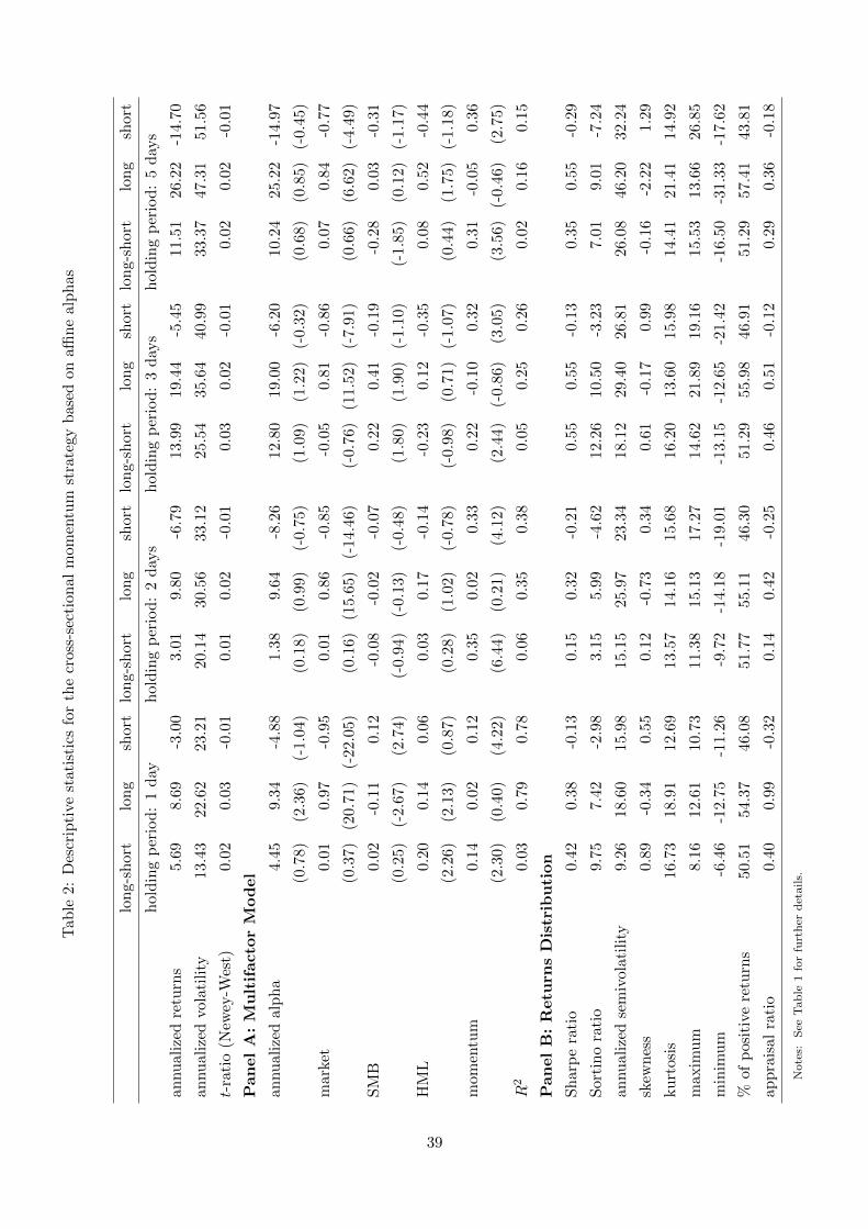
Tab
le2:
Des
crip
tive
stat
isti
csfo
rth
ecr
oss-
sect
ion
alm
omen
tum
stra
tegy
bas
edon
affin
eal
ph
as
lon
g-sh
ort
lon
gsh
ort
lon
g-sh
ort
long
shor
tlo
ng-
shor
tlo
ng
shor
tlo
ng-
shor
tlo
ng
shor
t
hol
din
gp
erio
d:
1d
ayh
old
ing
per
iod
:2
day
sh
old
ing
per
iod
:3
day
sh
old
ing
per
iod
:5
day
s
annu
aliz
edre
turn
s5.
698.
69-3
.00
3.01
9.80
-6.7
913
.99
19.4
4-5
.45
11.5
126
.22
-14.
70
annu
aliz
edvol
atil
ity
13.4
322.
6223
.21
20.1
430
.56
33.1
225
.54
35.6
440
.99
33.3
747
.31
51.5
6
t-ra
tio
(New
ey-W
est)
0.02
0.03
-0.0
10.
010.
02-0
.01
0.03
0.02
-0.0
10.
020.
02-0
.01
Pan
el
A:
Mu
ltif
acto
rM
od
el
annu
aliz
edal
ph
a4.4
59.3
4-4
.88
1.38
9.64
-8.2
612
.80
19.0
0-6
.20
10.2
425
.22
-14.
97
(0.7
8)
(2.3
6)(-
1.04
)(0
.18)
(0.9
9)(-
0.75
)(1
.09)
(1.2
2)(-
0.32
)(0
.68)
(0.8
5)(-
0.45
)
mark
et0.
010.
97-0
.95
0.01
0.86
-0.8
5-0
.05
0.81
-0.8
60.
070.
84-0
.77
(0.3
7)
(20.
71)
(-22
.05)
(0.1
6)(1
5.65
)(-
14.4
6)(-
0.76
)(1
1.52
)(-
7.91
)(0
.66)
(6.6
2)(-
4.49
)
SM
B0.0
2-0
.11
0.12
-0.0
8-0
.02
-0.0
70.
220.
41-0
.19
-0.2
80.
03-0
.31
(0.2
5)
(-2.6
7)(2
.74)
(-0.
94)
(-0.
13)
(-0.
48)
(1.8
0)(1
.90)
(-1.
10)
(-1.
85)
(0.1
2)(-
1.17
)
HM
L0.
200.
140.
060.
030.
17-0
.14
-0.2
30.
12-0
.35
0.08
0.52
-0.4
4
(2.2
6)
(2.1
3)(0
.87)
(0.2
8)(1
.02)
(-0.
78)
(-0.
98)
(0.7
1)(-
1.07
)(0
.44)
(1.7
5)(-
1.18
)
mom
entu
m0.
140.
020.
120.
350.
020.
330.
22-0
.10
0.32
0.31
-0.0
50.
36
(2.3
0)
(0.4
0)(4
.22)
(6.4
4)(0
.21)
(4.1
2)(2
.44)
(-0.
86)
(3.0
5)(3
.56)
(-0.
46)
(2.7
5)
R2
0.03
0.79
0.78
0.06
0.35
0.38
0.05
0.25
0.26
0.02
0.16
0.15
Pan
el
B:
Retu
rns
Dis
trib
uti
on
Sh
arp
era
tio
0.42
0.38
-0.1
30.
150.
32-0
.21
0.55
0.55
-0.1
30.
350.
55-0
.29
Sor
tin
ora
tio
9.75
7.42
-2.9
83.
155.
99-4
.62
12.2
610
.50
-3.2
37.
019.
01-7
.24
annu
aliz
edse
miv
ola
tili
ty9.
2618
.60
15.9
815
.15
25.9
723
.34
18.1
229
.40
26.8
126
.08
46.2
032
.24
skew
nes
s0.
89-0
.34
0.55
0.12
-0.7
30.
340.
61-0
.17
0.99
-0.1
6-2
.22
1.29
ku
rtosi
s16.
7318.
9112
.69
13.5
714
.16
15.6
816
.20
13.6
015
.98
14.4
121
.41
14.9
2
maxim
um
8.1
612.
6110
.73
11.3
815
.13
17.2
714
.62
21.8
919
.16
15.5
313
.66
26.8
5
min
imu
m-6
.46
-12.
75-1
1.26
-9.7
2-1
4.18
-19.
01-1
3.15
-12.
65-2
1.42
-16.
50-3
1.33
-17.
62
%of
posi
tive
retu
rns
50.5
154.
3746
.08
51.7
755
.11
46.3
051
.29
55.9
846
.91
51.2
957
.41
43.8
1
app
rais
alra
tio
0.4
00.
99-0
.32
0.14
0.42
-0.2
50.
460.
51-0
.12
0.29
0.36
-0.1
8
Note
s:S
eeT
ab
le1
for
furt
her
det
ail
s.
39

Tab
le3:
Des
crip
tive
stat
isti
csfo
rth
ecr
oss
-sec
tion
alm
omen
tum
stra
tegy
bas
edon
non
par
amet
ric
alp
has
,w
ith
risk
-fre
era
tead
just
men
t
lon
g-sh
ort
lon
gsh
ort
lon
g-sh
ort
long
shor
tlo
ng-
shor
tlo
ng
shor
tlo
ng-
shor
tlo
ng
shor
t
hol
din
gp
erio
d:
1d
ayh
old
ing
per
iod
:2
day
sh
old
ing
per
iod
:3
day
sh
old
ing
per
iod
:5
day
s
annu
aliz
edre
turn
s5.
078.
35-3
.27
12.7
114
.03
-1.3
312
.06
17.2
3-5
.17
6.47
22.4
2-1
5.95
annu
aliz
edvol
atil
ity
15.2
825.
4021
.12
20.9
633
.86
30.3
523
.87
41.1
435
.98
30.2
653
.53
44.3
6
t-ra
tio
(New
ey-W
est)
0.02
0.02
-0.0
10.
040.
02-0
.00
0.03
0.02
-0.0
10.
010.
01-0
.01
Pan
el
A:
Mu
ltif
acto
rM
od
el
annu
aliz
edal
ph
a4.0
39.0
4-5
.01
11.7
114
.31
-2.6
011
.35
16.9
3-5
.58
5.03
21.3
5-1
6.32
(0.6
9)
(1.7
7)(-
1.43
)(1
.54)
(1.4
2)(-
0.27
)(1
.15)
(0.9
8)(-
0.34
)(0
.37)
(0.6
5)(-
0.56
)
mark
et0.
091.
00-0
.91
-0.0
00.
84-0
.85
0.14
0.91
-0.7
60.
170.
85-0
.69
(1.8
9)
(15.
51)
(-24
.88)
(-0.
13)
(13.
96)
(-18
.24)
(1.8
8)(8
.47)
(-7.
89)
(2.2
2)(4
.87)
(-5.
22)
SM
B0.0
1-0
.11
0.12
0.27
0.18
0.10
0.21
0.41
-0.2
00.
170.
32-0
.15
(0.1
3)
(-1.8
2)(4
.01)
(2.8
0)(1
.23)
(0.8
7)(2
.03)
(2.0
0)(-
1.24
)(1
.44)
(1.2
4)(-
0.64
)
HM
L0.
600.
400.
200.
250.
31-0
.06
0.18
0.38
-0.2
00.
530.
71-0
.18
(5.2
9)
(3.9
9)(4
.55)
(2.3
1)(1
.68)
(-0.
35)
(1.1
5)(1
.25)
(-0.
91)
(2.2
0)(1
.65)
(-0.
66)
mom
entu
m-0
.07
-0.1
00.
04-0
.05
-0.2
30.
18-0
.04
-0.2
40.
20-0
.06
-0.2
50.
19
(-1.2
8)(-
2.55
)(1
.78)
(-0.
85)
(-3.
10)
(2.3
1)(-
0.37
)(-
1.66
)(2
.72)
(-0.
80)
(-1.
96)
(1.9
3)
R2
0.16
0.77
0.79
0.03
0.34
0.39
0.03
0.27
0.24
0.05
0.16
0.13
Pan
el
B:
Retu
rns
Dis
trib
uti
on
Sh
arp
era
tio
0.33
0.33
-0.1
50.
610.
41-0
.04
0.51
0.42
-0.1
40.
210.
42-0
.36
Sor
tin
ora
tio
7.45
6.31
-3.5
715
.36
8.08
-1.0
611
.38
7.55
-3.5
74.
296.
88-9
.11
annu
aliz
edse
miv
ola
tili
ty10
.81
21.
0114
.57
13.1
327
.56
19.9
116
.83
36.2
123
.00
23.9
551
.76
27.7
9
skew
nes
s1.
70-0
.26
0.30
2.81
0.11
0.93
1.31
-0.8
60.
77-0
.26
-1.9
50.
86
ku
rtosi
s41.
0321.
8810
.62
35.5
115
.70
16.3
824
.43
19.4
312
.05
13.0
219
.14
10.6
6
maxim
um
11.6
814.
748.
8514
.86
17.7
317
.81
18.3
223
.32
15.9
312
.95
17.4
020
.11
min
imu
m-9
.94
-15.
53-9
.89
-6.0
4-1
4.86
-15.
55-9
.07
-24.
47-1
6.76
-13.
03-3
0.12
-14.
96
%of
posi
tive
retu
rns
49.8
753.
4146
.40
50.4
255
.69
47.3
350
.84
55.6
645
.82
52.1
357
.02
44.0
7
app
rais
alra
tio
0.3
50.
71-0
.45
0.69
0.56
-0.0
70.
500.
40-0
.13
0.19
0.27
-0.2
2
Note
s:S
eeT
ab
le1
for
furt
her
det
ail
s.
40
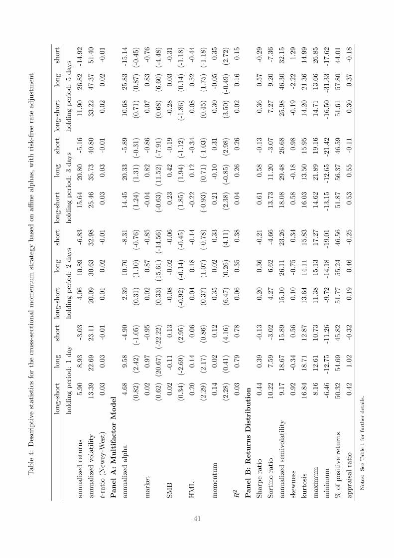
Tab
le4:
Des
crip
tive
stat
isti
csfo
rth
ecr
oss-
sect
ion
alm
omen
tum
stra
tegy
bas
edon
affin
eal
ph
as,
wit
hri
sk-f
ree
rate
adju
stm
ent
lon
g-sh
ort
lon
gsh
ort
lon
g-sh
ort
long
shor
tlo
ng-
shor
tlo
ng
shor
tlo
ng-
shor
tlo
ng
shor
t
hol
din
gp
erio
d:
1d
ayh
old
ing
per
iod
:2
day
sh
old
ing
per
iod
:3
day
sh
old
ing
per
iod
:5
day
s
annu
aliz
edre
turn
s5.
908.
93-3
.03
4.06
10.8
9-6
.83
15.6
420
.80
-5.1
611
.90
26.8
2-1
4.92
annu
aliz
edvol
atil
ity
13.3
922.
6923
.11
20.0
930
.63
32.9
825
.46
35.7
340
.80
33.2
247
.37
51.4
0
t-ra
tio
(New
ey-W
est)
0.03
0.03
-0.0
10.
010.
02-0
.01
0.03
0.03
-0.0
10.
020.
02-0
.01
Pan
el
A:
Mu
ltif
acto
rM
od
el
annu
aliz
edal
ph
a4.6
89.5
8-4
.90
2.39
10.7
0-8
.31
14.4
520
.33
-5.8
910
.68
25.8
3-1
5.14
(0.8
2)
(2.4
2)(-
1.05
)(0
.31)
(1.1
0)(-
0.76
)(1
.24)
(1.3
1)(-
0.31
)(0
.71)
(0.8
7)(-
0.45
)
mark
et0.
020.
97-0
.95
0.02
0.87
-0.8
5-0
.04
0.82
-0.8
60.
070.
83-0
.76
(0.6
2)
(20.
67)
(-22
.22)
(0.3
3)(1
5.61
)(-
14.5
6)(-
0.63
)(1
1.52
)(-
7.91
)(0
.68)
(6.6
0)(-
4.48
)
SM
B0.0
2-0
.11
0.13
-0.0
8-0
.02
-0.0
60.
230.
42-0
.19
-0.2
80.
03-0
.31
(0.3
4)
(-2.6
9)(2
.95)
(-0.
92)
(-0.
14)
(-0.
45)
(1.8
5)(1
.94)
(-1.
12)
(-1.
86)
(0.1
4)(-
1.18
)
HM
L0.
200.
140.
060.
040.
18-0
.14
-0.2
20.
12-0
.34
0.08
0.52
-0.4
4
(2.2
9)
(2.1
7)(0
.86)
(0.3
7)(1
.07)
(-0.
78)
(-0.
93)
(0.7
1)(-
1.03
)(0
.45)
(1.7
5)(-
1.18
)
mom
entu
m0.
140.
020.
120.
350.
020.
330.
21-0
.10
0.31
0.30
-0.0
50.
35
(2.2
8)
(0.4
1)(4
.16)
(6.4
7)(0
.26)
(4.1
1)(2
.38)
(-0.
85)
(2.9
8)(3
.50)
(-0.
49)
(2.7
2)
R2
0.03
0.79
0.78
0.06
0.35
0.38
0.04
0.26
0.26
0.02
0.16
0.15
Pan
el
B:
Retu
rns
Dis
trib
uti
on
Sh
arp
era
tio
0.44
0.39
-0.1
30.
200.
36-0
.21
0.61
0.58
-0.1
30.
360.
57-0
.29
Sor
tin
ora
tio
10.
227.
59-3
.02
4.27
6.62
-4.6
613
.73
11.2
0-3
.07
7.27
9.20
-7.3
6
annu
aliz
edse
miv
ola
tili
ty9.
1718
.67
15.8
915
.10
26.1
123
.26
18.0
829
.48
26.6
825
.98
46.3
032
.15
skew
nes
s0.
92-0
.34
0.56
0.10
-0.7
50.
340.
58-0
.18
0.98
-0.1
9-2
.22
1.29
ku
rtosi
s16.
8418.
7112
.87
13.6
414
.11
15.8
316
.03
13.5
015
.95
14.2
021
.36
14.9
9
maxim
um
8.1
612.
6110
.73
11.3
815
.13
17.2
714
.62
21.8
919
.16
14.7
113
.66
26.8
5
min
imu
m-6
.46
-12.
75-1
1.26
-9.7
2-1
4.18
-19.
01-1
3.15
-12.
65-2
1.42
-16.
50-3
1.33
-17.
62
%of
posi
tive
retu
rns
50.3
254.
6945
.82
51.7
755
.24
46.5
651
.87
56.3
746
.59
51.6
157
.80
44.0
1
app
rais
alra
tio
0.4
21.
02-0
.32
0.19
0.46
-0.2
50.
530.
55-0
.11
0.30
0.37
-0.1
8
Note
s:S
eeT
ab
le1
for
furt
her
det
ail
s.
41
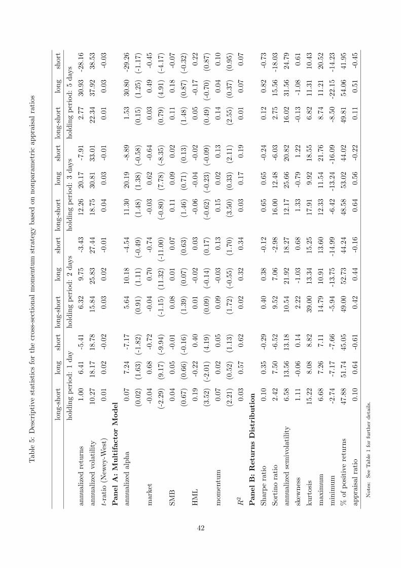
Tab
le5:
Des
crip
tive
stati
stic
sfo
rth
ecr
oss-
sect
ion
alm
omen
tum
stra
tegy
bas
edon
non
par
amet
ric
app
rais
alra
tios
lon
g-sh
ort
lon
gsh
ort
lon
g-sh
ort
lon
gsh
ort
lon
g-sh
ort
lon
gsh
ort
lon
g-sh
ort
lon
gsh
ort
hol
din
gp
erio
d:
1d
ayh
old
ing
per
iod
:2
day
sh
old
ing
per
iod
:3
day
sh
old
ing
per
iod
:5
day
s
annu
aliz
edre
turn
s1.
006.4
1-5
.41
6.32
9.75
-3.4
312
.26
20.1
7-7
.91
2.77
30.9
3-2
8.16
annu
aliz
edvol
atil
ity
10.2
718.
1718
.78
15.8
425
.83
27.4
418
.75
30.8
133
.01
22.3
437
.92
38.5
3
t-ra
tio
(New
ey-W
est)
0.01
0.0
2-0
.02
0.03
0.02
-0.0
10.
040.
03-0
.01
0.01
0.03
-0.0
3
Pan
el
A:
Mu
ltif
acto
rM
od
el
annu
aliz
edal
ph
a0.0
77.
24-7
.17
5.64
10.1
8-4
.54
11.3
020
.19
-8.8
91.
5330
.80
-29.
26
(0.0
2)
(1.6
3)(-
1.82
)(0
.91)
(1.1
1)(-
0.49
)(1
.48)
(1.3
8)(-
0.58
)(0
.15)
(1.2
5)(-
1.17
)
mark
et-0
.04
0.68
-0.7
2-0
.04
0.70
-0.7
4-0
.03
0.62
-0.6
40.
030.
49-0
.45
(-2.2
9)(9
.17)
(-9.
94)
(-1.
15)
(11.
32)
(-11
.00)
(-0.
80)
(7.7
8)(-
8.35
)(0
.79)
(4.9
1)(-
4.17
)
SM
B0.0
40.
05-0
.01
0.08
0.01
0.07
0.11
0.09
0.02
0.11
0.18
-0.0
7
(0.6
7)
(0.6
6)(-
0.16
)(1
.39)
(0.0
7)(0
.63)
(1.4
6)(0
.71)
(0.1
3)(1
.48)
(0.8
7)(-
0.32
)
HM
L0.
19-0
.22
0.40
0.01
-0.0
20.
03-0
.06
-0.0
4-0
.02
0.05
-0.1
70.
22
(3.5
2)
(-2.
01)
(4.1
9)(0
.09)
(-0.
14)
(0.1
7)(-
0.62
)(-
0.23
)(-
0.09
)(0
.49)
(-0.
70)
(0.8
7)
mom
entu
m0.
070.0
20.
050.
09-0
.03
0.13
0.15
0.02
0.13
0.14
0.04
0.10
(2.2
1)
(0.5
2)(1
.13)
(1.7
2)(-
0.55
)(1
.70)
(3.5
0)(0
.33)
(2.1
1)(2
.55)
(0.3
7)(0
.95)
R2
0.0
30.
570.
620.
020.
320.
340.
030.
170.
190.
010.
070.
07
Pan
el
B:
Retu
rns
Dis
trib
uti
on
Sh
arp
era
tio
0.10
0.3
5-0
.29
0.40
0.38
-0.1
20.
650.
65-0
.24
0.12
0.82
-0.7
3
Sor
tin
ora
tio
2.42
7.5
0-6
.52
9.52
7.06
-2.9
816
.00
12.4
8-6
.03
2.75
15.5
6-1
8.03
annu
aliz
edse
miv
ola
tili
ty6.
5813
.56
13.1
810
.54
21.9
218
.27
12.1
725
.66
20.8
216
.02
31.5
624
.79
skew
nes
s1.
11-0
.06
0.14
2.22
-1.0
30.
681.
33-0
.79
1.22
-0.1
3-1
.08
0.61
ku
rtosi
s15.
228.0
88.
8239
.00
13.3
415
.25
17.9
19.
9218
.55
6.82
11.3
110
.43
maxim
um
6.6
87.
267.
1114
.79
10.9
113
.60
12.3
311
.54
21.7
68.
7411
.21
20.5
2
min
imu
m-2
.74
-7.1
7-7
.66
-5.9
4-1
3.75
-14.
99-6
.42
-13.
24-1
6.09
-8.5
0-2
2.15
-14.
23
%of
posi
tive
retu
rns
47.8
851.
7445
.05
49.0
052
.73
44.2
448
.58
53.0
244
.02
49.8
154
.06
41.9
5
app
rais
alra
tio
0.1
00.
64-0
.61
0.42
0.44
-0.1
60.
640.
56-0
.22
0.11
0.51
-0.4
5
Note
s:S
eeT
ab
le1
for
furt
her
det
ail
s.
42
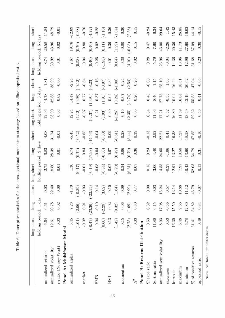
Tab
le6:
Des
crip
tive
stat
isti
csfo
rth
ecr
oss-
sect
ion
alm
omen
tum
stra
tegy
bas
edon
affin
eap
pra
isal
rati
os
lon
g-sh
ort
lon
gsh
ort
lon
g-sh
ort
long
shor
tlo
ng-
shor
tlo
ng
shor
tlo
ng-
shor
tlo
ng
shor
t
hol
din
gp
erio
d:
1d
ayh
old
ing
per
iod
:2
day
sh
old
ing
per
iod
:3
day
sh
old
ing
per
iod
:5
day
s
annu
aliz
edre
turn
s6.
646.
610.
032.
756.
83-4
.08
12.9
614
.78
-1.8
18.
7420
.58
-11.
84
annu
aliz
edvol
atil
ity
12.6
120.
7822
.40
18.8
028
.39
31.7
423
.90
32.8
838
.99
30.9
243
.96
48.7
9
t-ra
tio
(New
ey-W
est)
0.03
0.02
0.00
0.01
0.01
-0.0
10.
030.
02-0
.00
0.01
0.02
-0.0
1
Pan
el
A:
Mu
ltif
acto
rM
od
el
annu
aliz
edal
ph
a5.4
57.2
3-1
.79
1.30
6.74
-5.4
512
.24
14.4
7-2
.24
7.67
19.7
6-1
2.09
(1.0
4)
(2.0
6)(-
0.39
)(0
.17)
(0.7
4)(-
0.52
)(1
.12)
(0.9
8)(-
0.12
)(0
.53)
(0.7
0)(-
0.38
)
mark
et-0
.02
0.91
-0.9
3-0
.01
0.84
-0.8
5-0
.07
0.77
-0.8
40.
040.
80-0
.76
(-0.4
7)(2
3.3
6)(-
22.5
5)(-
0.19
)(1
7.98
)(-
14.5
3)(-
1.37
)(1
0.91
)(-
8.23
)(0
.40)
(6.4
0)(-
4.72
)
SM
B0.0
4-0
.10
0.14
-0.0
8-0
.04
-0.0
40.
210.
37-0
.16
-0.2
50.
02-0
.28
(0.6
0)
(-2.2
9)(3
.02)
(-0.
84)
(-0.
36)
(-0.
30)
(1.9
3)(1
.91)
(-0.
97)
(-1.
95)
(0.1
1)(-
1.10
)
HM
L0.
130.
020.
10-0
.02
0.07
-0.0
9-0
.30
0.04
-0.3
40.
010.
36-0
.36
(1.4
2)
(0.3
2)(1
.64)
(-0.
20)
(0.4
9)(-
0.51
)(-
1.25
)(0
.24)
(-1.
00)
(0.0
4)(1
.29)
(-1.
04)
mom
entu
m0.
150.
060.
090.
340.
060.
280.
16-0
.07
0.24
0.30
-0.0
00.
30
(2.7
5)
(1.6
9)(2
.99)
(6.6
1)(0
.79)
(3.4
4)(2
.35)
(-0.
74)
(2.5
4)(4
.10)
(-0.
03)
(2.5
8)
R2
0.03
0.80
0.77
0.07
0.36
0.39
0.05
0.26
0.26
0.02
0.15
0.15
Pan
el
B:
Retu
rns
Dis
trib
uti
on
Sh
arp
era
tio
0.53
0.32
0.00
0.15
0.24
-0.1
30.
540.
45-0
.05
0.28
0.47
-0.2
4
Sor
tin
ora
tio
11.
806.
150.
033.
004.
40-2
.92
11.9
68.
46-1
.15
5.79
7.60
-6.3
4
annu
aliz
edse
miv
ola
tili
ty8.
9317
.08
15.2
414
.55
24.6
522
.21
17.2
127
.73
25.1
023
.96
43.0
029
.64
skew
nes
s0.
53-0
.56
0.57
-0.2
7-1
.06
0.41
0.52
-0.5
51.
03-0
.04
-2.2
61.
42
ku
rtosi
s16.
3015.
5013
.14
12.9
113
.27
16.3
816
.80
10.9
416
.24
14.3
620
.36
15.4
3
maxim
um
6.4
89.
6610
.88
7.97
10.5
817
.27
11.5
916
.84
18.8
113
.96
11.7
326
.85
min
imu
m-6
.78
-12.
80-1
1.12
-10.
43-1
3.60
-18.
58-1
3.49
-12.
19-2
0.62
-12.
96-2
7.60
-16.
02
%of
posi
tive
retu
rns
51.4
154.
8246
.79
52.0
354
.79
47.8
552
.32
55.5
347
.04
51.6
857
.09
44.1
4
app
rais
alra
tio
0.4
90.
84-0
.07
0.13
0.31
-0.1
60.
460.
41-0
.05
0.23
0.30
-0.1
5
Note
s:S
eeT
ab
le1
for
furt
her
det
ail
s.
43
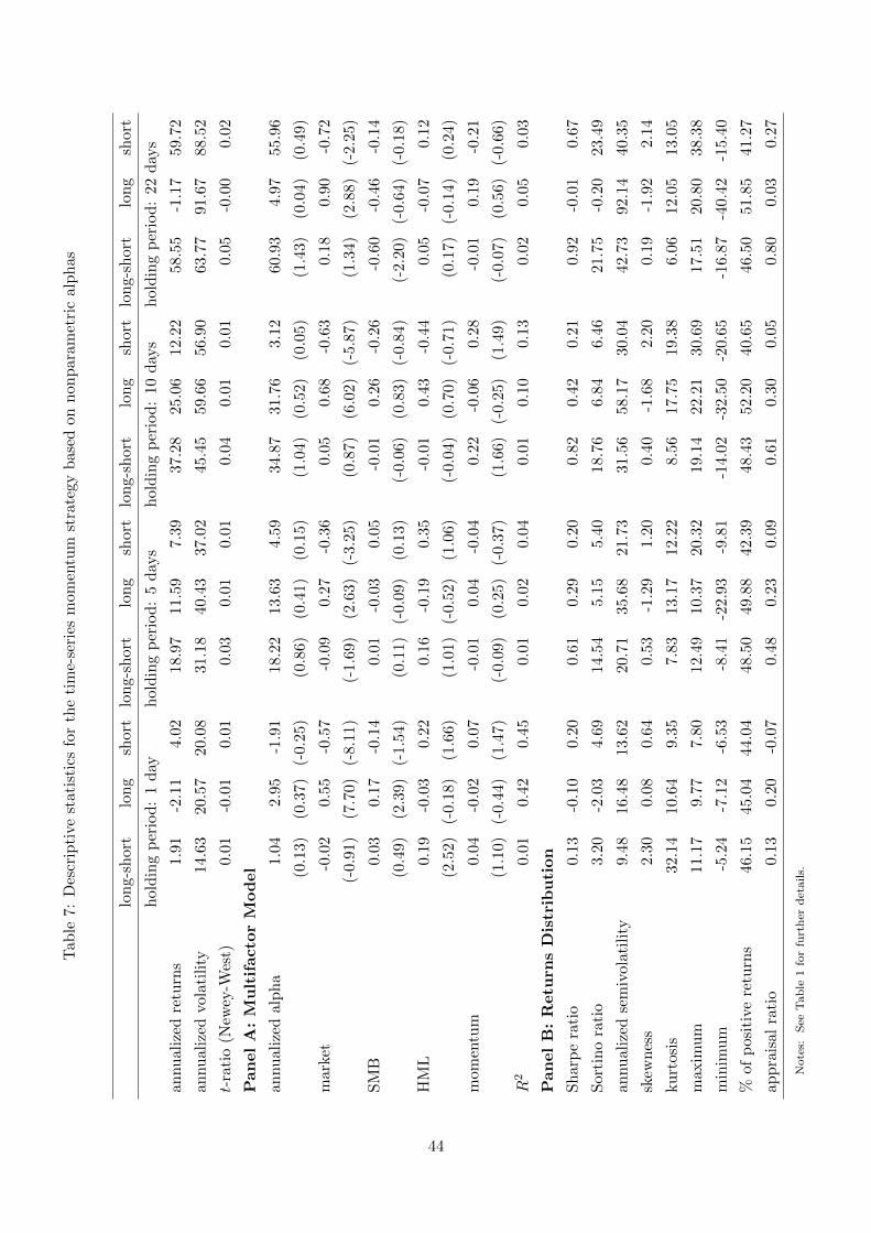
Tab
le7:
Des
crip
tive
stati
stic
sfo
rth
eti
me-
seri
esm
omen
tum
stra
tegy
bas
edon
non
par
amet
ric
alp
has
lon
g-s
hort
lon
gsh
ort
lon
g-sh
ort
lon
gsh
ort
lon
g-sh
ort
lon
gsh
ort
lon
g-sh
ort
long
shor
t
hold
ing
per
iod
:1
day
hol
din
gp
erio
d:
5d
ays
hol
din
gp
erio
d:
10d
ays
hol
din
gp
erio
d:
22d
ays
an
nu
ali
zed
retu
rns
1.9
1-2
.11
4.02
18.9
711
.59
7.39
37.2
825
.06
12.2
258
.55
-1.1
759
.72
an
nu
ali
zed
vola
tility
14.
6320
.57
20.0
831
.18
40.4
337
.02
45.4
559
.66
56.9
063
.77
91.6
788
.52
t-ra
tio
(New
ey-W
est)
0.01
-0.0
10.
010.
030.
010.
010.
040.
010.
010.
05-0
.00
0.02
Pan
el
A:
Mu
ltif
acto
rM
od
el
an
nu
ali
zed
alp
ha
1.04
2.9
5-1
.91
18.2
213
.63
4.59
34.8
731
.76
3.12
60.9
34.
9755
.96
(0.1
3)(0
.37)
(-0.
25)
(0.8
6)(0
.41)
(0.1
5)(1
.04)
(0.5
2)(0
.05)
(1.4
3)(0
.04)
(0.4
9)
mar
ket
-0.0
20.5
5-0
.57
-0.0
90.
27-0
.36
0.05
0.68
-0.6
30.
180.
90-0
.72
(-0.9
1)(7
.70)
(-8.
11)
(-1.
69)
(2.6
3)(-
3.25
)(0
.87)
(6.0
2)(-
5.87
)(1
.34)
(2.8
8)(-
2.25
)
SM
B0.
030.1
7-0
.14
0.01
-0.0
30.
05-0
.01
0.26
-0.2
6-0
.60
-0.4
6-0
.14
(0.4
9)(2
.39)
(-1.
54)
(0.1
1)(-
0.09
)(0
.13)
(-0.
06)
(0.8
3)(-
0.84
)(-
2.20
)(-
0.64
)(-
0.18
)
HM
L0.1
9-0
.03
0.22
0.16
-0.1
90.
35-0
.01
0.43
-0.4
40.
05-0
.07
0.12
(2.5
2)(-
0.1
8)(1
.66)
(1.0
1)(-
0.52
)(1
.06)
(-0.
04)
(0.7
0)(-
0.71
)(0
.17)
(-0.
14)
(0.2
4)
mom
entu
m0.0
4-0
.02
0.07
-0.0
10.
04-0
.04
0.22
-0.0
60.
28-0
.01
0.19
-0.2
1
(1.1
0)(-
0.4
4)(1
.47)
(-0.
09)
(0.2
5)(-
0.37
)(1
.66)
(-0.
25)
(1.4
9)(-
0.07
)(0
.56)
(-0.
66)
R2
0.01
0.4
20.
450.
010.
020.
040.
010.
100.
130.
020.
050.
03
Pan
el
B:
Retu
rns
Dis
trib
uti
on
Sh
arp
era
tio
0.13
-0.1
00.
200.
610.
290.
200.
820.
420.
210.
92-0
.01
0.67
Sor
tin
ora
tio
3.20
-2.0
34.
6914
.54
5.15
5.40
18.7
66.
846.
4621
.75
-0.2
023
.49
annu
aliz
edse
miv
ola
tili
ty9.
4816
.48
13.6
220
.71
35.6
821
.73
31.5
658
.17
30.0
442
.73
92.1
440
.35
skew
nes
s2.
300.0
80.
640.
53-1
.29
1.20
0.40
-1.6
82.
200.
19-1
.92
2.14
ku
rtosi
s32.
1410
.64
9.35
7.83
13.1
712
.22
8.56
17.7
519
.38
6.06
12.0
513
.05
maxim
um
11.1
79.
777.
8012
.49
10.3
720
.32
19.1
422
.21
30.6
917
.51
20.8
038
.38
min
imu
m-5
.24
-7.1
2-6
.53
-8.4
1-2
2.93
-9.8
1-1
4.02
-32.
50-2
0.65
-16.
87-4
0.42
-15.
40
%of
posi
tive
retu
rns
46.1
545.
0444
.04
48.5
049
.88
42.3
948
.43
52.2
040
.65
46.5
051
.85
41.2
7
app
rais
alra
tio
0.1
30.
20-0
.07
0.48
0.23
0.09
0.61
0.30
0.05
0.80
0.03
0.27
Note
s:S
eeT
ab
le1
for
furt
her
det
ails.
44
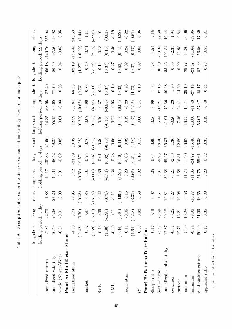
Tab
le8:
Des
crip
tive
stat
isti
csfo
rth
eti
me-
seri
esm
omen
tum
stra
tegy
bas
edon
affin
eal
ph
as
lon
g-s
hort
lon
gsh
ort
lon
g-sh
ort
lon
gsh
ort
lon
g-sh
ort
lon
gsh
ort
lon
g-sh
ort
lon
gsh
ort
hold
ing
per
iod
:1
day
hol
din
gp
erio
d:
5d
ays
hol
din
gp
erio
d:
10d
ays
hol
din
gp
erio
d:
22d
ays
an
nu
ali
zed
retu
rns
-2.8
1-4
.70
1.88
10.1
7-3
0.83
41.0
014
.35
-68.
0582
.40
106.
18-1
49.7
625
5.94
an
nu
ali
zed
vola
tili
ty16.
5924
.08
27.2
040
.34
48.5
259
.25
55.1
568
.65
77.7
686
.49
97.5
011
8.92
t-ra
tio
(New
ey-W
est)
-0.0
1-0
.01
0.00
0.01
-0.0
20.
020.
01-0
.03
0.03
0.04
-0.0
30.
05
Pan
el
A:
Mu
ltif
acto
rM
od
el
an
nu
ali
zed
alp
ha
-4.2
03.
74-7
.95
6.42
-23.
8930
.32
12.5
9-5
5.84
68.4
310
2.19
-146
.44
248.
63
(-0.4
2)(0
.70)
(-0.
88)
(0.2
5)(-
0.57
)(0
.58)
(0.3
0)(-
0.67
)(0
.73)
(1.2
7)(-
0.99
)(1
.44)
mark
et0.
020.
87-0
.85
-0.0
10.
75-0
.76
0.07
0.90
-0.8
3-0
.40
0.71
-1.1
1
(0.6
9)
(15.
13)
(-15
.12)
(-0.
08)
(4.4
6)(-
3.54
)(0
.37)
(6.3
6)(-
3.33
)(-
2.72
)(2
.35)
(-2.
95)
SM
B0.1
3-0
.09
0.22
-0.3
60.
01-0
.36
-0.1
6-0
.37
0.22
0.14
0.13
0.01
(1.8
0)
(-1.9
8)(3
.75)
(-1.
71)
(0.0
2)(-
0.70
)(-
0.48
)(-
0.88
)(0
.37)
(0.3
7)(0
.18)
(0.0
1)
HM
L-0
.00
0.11
-0.1
10.
340.
280.
060.
220.
030.
190.
270.
46-0
.19
(-0.0
4)(1
.40)
(-0.
99)
(1.2
5)(0
.70)
(0.1
1)(0
.60)
(0.0
5)(0
.32)
(0.6
2)(0
.62)
(-0.
32)
mom
entu
m0.
11-0
.05
0.16
0.29
-0.0
30.
320.
19-0
.29
0.48
0.02
0.24
-0.2
2
(1.6
4)
(-1.2
8)(3
.32)
(2.6
5)(-
0.21
)(1
.78)
(0.9
7)(-
1.15
)(1
.70)
(0.0
7)(0
.77)
(-0.
61)
R2
0.02
0.82
0.68
0.02
0.16
0.13
0.00
0.14
0.10
0.02
0.04
0.06
Pan
el
B:
Retu
rns
Dis
trib
uti
on
Sh
arp
era
tio
-0.1
7-0
.19
0.07
0.25
-0.6
40.
690.
26-0
.99
1.06
1.23
-1.5
42.
15
Sor
tin
ora
tio
-3.4
7-3
.69
1.51
5.31
-9.9
318
.40
5.44
-14.
2432
.16
30.4
0-2
3.34
87.5
0
annu
aliz
edse
miv
ola
tili
ty12
.87
20.
1819
.81
30.3
849
.27
35.3
741
.91
75.8
640
.68
55.4
610
1.84
46.4
4
skew
nes
s-0
.51
-0.2
50.
27-0
.21
-2.3
31.
36-0
.20
-3.2
31.
900.
55-2
.35
1.94
ku
rtosi
s12.
7113.
2110
.98
6.68
16.8
112
.89
7.46
24.4
114
.80
6.99
11.9
89.
84
maxim
um
5.0
910.
289.
5311
.74
11.2
026
.02
16.5
515
.71
39.1
929
.77
11.8
050
.06
min
imu
m-8
.94
-9.9
8-1
0.77
-11.
85-2
4.77
-15.
48-1
8.80
-41.
43-2
7.14
-23.
87-4
1.64
-19.
95
%of
posi
tive
retu
rns
50.0
051.
9946
.65
51.7
555
.61
46.3
853
.07
57.4
745
.17
52.9
956
.56
47.3
9
app
rais
alra
tio
-0.1
70.3
5-0
.39
0.20
-0.3
20.
350.
19-0
.40
0.44
0.73
-0.5
50.
81
Note
s:S
eeT
ab
le1
for
furt
her
det
ail
s.
45
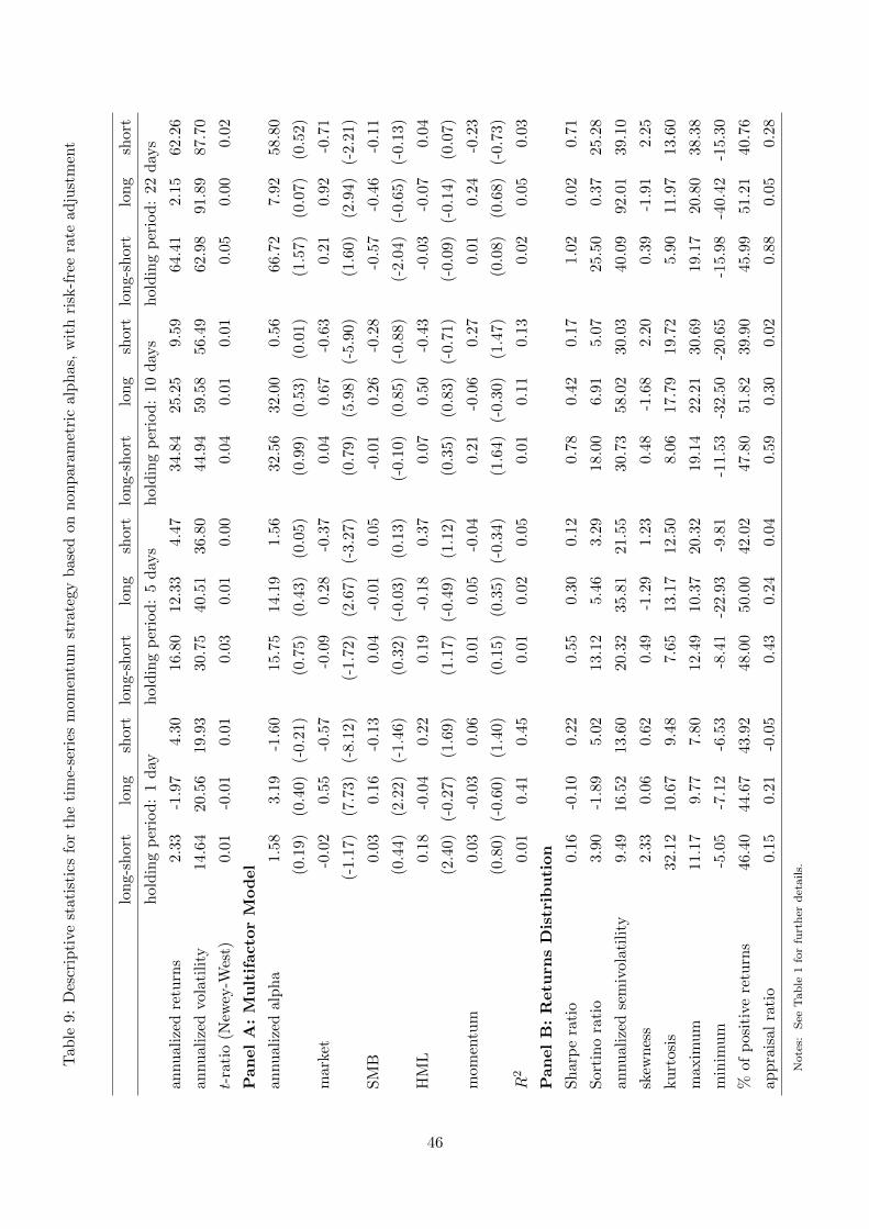
Tab
le9:
Des
crip
tive
stat
isti
csfo
rth
eti
me-
seri
esm
omen
tum
stra
tegy
bas
edon
non
par
amet
ric
alp
has
,w
ith
risk
-fre
era
tead
just
men
t
lon
g-s
hort
lon
gsh
ort
lon
g-sh
ort
lon
gsh
ort
lon
g-sh
ort
lon
gsh
ort
lon
g-sh
ort
long
shor
t
hold
ing
per
iod
:1
day
hol
din
gp
erio
d:
5d
ays
hol
din
gp
erio
d:
10d
ays
hol
din
gp
erio
d:
22d
ays
an
nu
ali
zed
retu
rns
2.3
3-1
.97
4.30
16.8
012
.33
4.47
34.8
425
.25
9.59
64.4
12.
1562
.26
an
nu
ali
zed
vola
tility
14.
6420
.56
19.9
330
.75
40.5
136
.80
44.9
459
.58
56.4
962
.98
91.8
987
.70
t-ra
tio
(New
ey-W
est)
0.01
-0.0
10.
010.
030.
010.
000.
040.
010.
010.
050.
000.
02
Pan
el
A:
Mu
ltif
acto
rM
od
el
an
nu
ali
zed
alp
ha
1.58
3.1
9-1
.60
15.7
514
.19
1.56
32.5
632
.00
0.56
66.7
27.
9258
.80
(0.1
9)(0
.40)
(-0.
21)
(0.7
5)(0
.43)
(0.0
5)(0
.99)
(0.5
3)(0
.01)
(1.5
7)(0
.07)
(0.5
2)
mar
ket
-0.0
20.5
5-0
.57
-0.0
90.
28-0
.37
0.04
0.67
-0.6
30.
210.
92-0
.71
(-1.1
7)(7
.73)
(-8.
12)
(-1.
72)
(2.6
7)(-
3.27
)(0
.79)
(5.9
8)(-
5.90
)(1
.60)
(2.9
4)(-
2.21
)
SM
B0.
030.1
6-0
.13
0.04
-0.0
10.
05-0
.01
0.26
-0.2
8-0
.57
-0.4
6-0
.11
(0.4
4)(2
.22)
(-1.
46)
(0.3
2)(-
0.03
)(0
.13)
(-0.
10)
(0.8
5)(-
0.88
)(-
2.04
)(-
0.65
)(-
0.13
)
HM
L0.1
8-0
.04
0.22
0.19
-0.1
80.
370.
070.
50-0
.43
-0.0
3-0
.07
0.04
(2.4
0)(-
0.2
7)(1
.69)
(1.1
7)(-
0.49
)(1
.12)
(0.3
5)(0
.83)
(-0.
71)
(-0.
09)
(-0.
14)
(0.0
7)
mom
entu
m0.0
3-0
.03
0.06
0.01
0.05
-0.0
40.
21-0
.06
0.27
0.01
0.24
-0.2
3
(0.8
0)(-
0.6
0)(1
.40)
(0.1
5)(0
.35)
(-0.
34)
(1.6
4)(-
0.30
)(1
.47)
(0.0
8)(0
.68)
(-0.
73)
R2
0.01
0.4
10.
450.
010.
020.
050.
010.
110.
130.
020.
050.
03
Pan
el
B:
Retu
rns
Dis
trib
uti
on
Sh
arp
era
tio
0.16
-0.1
00.
220.
550.
300.
120.
780.
420.
171.
020.
020.
71
Sor
tin
ora
tio
3.90
-1.8
95.
0213
.12
5.46
3.29
18.0
06.
915.
0725
.50
0.37
25.2
8
annu
aliz
edse
miv
ola
tili
ty9.
4916
.52
13.6
020
.32
35.8
121
.55
30.7
358
.02
30.0
340
.09
92.0
139
.10
skew
nes
s2.
330.0
60.
620.
49-1
.29
1.23
0.48
-1.6
82.
200.
39-1
.91
2.25
ku
rtosi
s32.
1210
.67
9.48
7.65
13.1
712
.50
8.06
17.7
919
.72
5.90
11.9
713
.60
maxim
um
11.1
79.
777.
8012
.49
10.3
720
.32
19.1
422
.21
30.6
919
.17
20.8
038
.38
min
imu
m-5
.05
-7.1
2-6
.53
-8.4
1-2
2.93
-9.8
1-1
1.53
-32.
50-2
0.65
-15.
98-4
0.42
-15.
30
%of
posi
tive
retu
rns
46.4
044.
6743
.92
48.0
050
.00
42.0
247
.80
51.8
239
.90
45.9
951
.21
40.7
6
app
rais
alra
tio
0.1
50.
21-0
.05
0.43
0.24
0.04
0.59
0.30
0.02
0.88
0.05
0.28
Note
s:S
eeT
ab
le1
for
furt
her
det
ails.
46
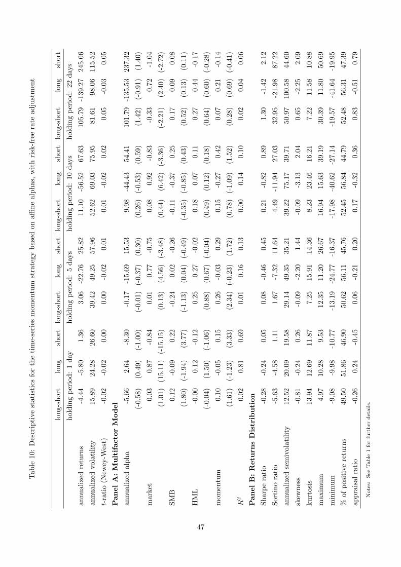
Tab
le10:
Des
crip
tive
stat
isti
csfo
rth
eti
me-
seri
esm
omen
tum
stra
tegy
bas
edon
affin
eal
ph
as,
wit
hri
sk-f
ree
rate
adju
stm
ent
lon
g-s
hort
lon
gsh
ort
lon
g-sh
ort
lon
gsh
ort
lon
g-sh
ort
lon
gsh
ort
lon
g-sh
ort
lon
gsh
ort
hold
ing
per
iod
:1
day
hol
din
gp
erio
d:
5d
ays
hol
din
gp
erio
d:
10d
ays
hol
din
gp
erio
d:
22d
ays
an
nu
ali
zed
retu
rns
-4.4
4-5
.80
1.36
3.06
-22.
7625
.82
11.1
0-5
6.52
67.6
310
5.79
-139
.27
245.
06
an
nu
ali
zed
vola
tili
ty15.
8924
.28
26.6
039
.42
49.2
557
.96
52.6
269
.03
75.9
581
.61
98.0
611
5.52
t-ra
tio
(New
ey-W
est)
-0.0
2-0
.02
0.00
0.00
-0.0
20.
010.
01-0
.02
0.02
0.05
-0.0
30.
05
Pan
el
A:
Mu
ltif
acto
rM
od
el
an
nu
ali
zed
alp
ha
-5.6
62.
64-8
.30
-0.1
7-1
5.69
15.5
39.
98-4
4.43
54.4
110
1.79
-135
.53
237.
32
(-0.5
8)(0
.49)
(-1.
00)
(-0.
01)
(-0.
37)
(0.3
0)(0
.26)
(-0.
53)
(0.5
9)(1
.42)
(-0.
91)
(1.4
0)
mark
et0.
030.
87-0
.84
0.01
0.77
-0.7
50.
080.
92-0
.83
-0.3
30.
72-1
.04
(1.0
1)
(15.
11)
(-15
.15)
(0.1
3)(4
.56)
(-3.
48)
(0.4
4)(6
.42)
(-3.
36)
(-2.
21)
(2.4
0)(-
2.72
)
SM
B0.1
2-0
.09
0.22
-0.2
40.
02-0
.26
-0.1
1-0
.37
0.25
0.17
0.09
0.08
(1.8
0)
(-1.9
4)(3
.77)
(-1.
13)
(0.0
4)(-
0.49
)(-
0.35
)(-
0.85
)(0
.43)
(0.5
2)(0
.13)
(0.1
1)
HM
L-0
.00
0.12
-0.1
20.
250.
27-0
.02
0.18
0.07
0.11
0.27
0.44
-0.1
7
(-0.0
4)(1
.50)
(-1.
06)
(0.8
8)(0
.67)
(-0.
04)
(0.4
9)(0
.12)
(0.1
8)(0
.64)
(0.6
0)(-
0.28
)
mom
entu
m0.
10-0
.05
0.15
0.26
-0.0
30.
290.
15-0
.27
0.42
0.07
0.21
-0.1
4
(1.6
1)
(-1.2
3)(3
.33)
(2.3
4)(-
0.23
)(1
.72)
(0.7
8)(-
1.09
)(1
.52)
(0.2
8)(0
.69)
(-0.
41)
R2
0.02
0.81
0.69
0.01
0.16
0.13
0.00
0.14
0.10
0.02
0.04
0.06
Pan
el
B:
Retu
rns
Dis
trib
uti
on
Sh
arp
era
tio
-0.2
8-0
.24
0.05
0.08
-0.4
60.
450.
21-0
.82
0.89
1.30
-1.4
22.
12
Sor
tin
ora
tio
-5.6
3-4
.58
1.11
1.67
-7.3
211
.64
4.49
-11.
9427
.03
32.9
5-2
1.98
87.2
2
annu
aliz
edse
miv
ola
tili
ty12
.52
20.
0919
.58
29.1
449
.35
35.2
139
.22
75.1
739
.71
50.9
710
0.58
44.6
0
skew
nes
s-0
.81
-0.2
40.
26-0
.09
-2.2
01.
44-0
.09
-3.1
32.
040.
65-2
.25
2.09
ku
rtosi
s13.
9412.
6911
.87
7.25
15.9
114
.36
8.23
23.4
616
.21
7.22
11.5
810
.88
maxim
um
4.9
710.
289.
5312
.35
11.2
026
.67
16.9
415
.63
39.1
930
.39
11.8
050
.69
min
imu
m-9
.08
-9.9
8-1
0.77
-13.
19-2
4.77
-16.
37-1
7.98
-40.
62-2
7.14
-19.
57-4
1.64
-19.
95
%of
posi
tive
retu
rns
49.5
051.
8646
.90
50.6
256
.11
45.7
652
.45
56.8
444
.79
52.4
856
.31
47.3
9
app
rais
alra
tio
-0.2
60.2
4-0
.45
0.06
-0.2
10.
200.
17-0
.32
0.36
0.83
-0.5
10.
79
Note
s:S
eeT
ab
le1
for
furt
her
det
ail
s.
47
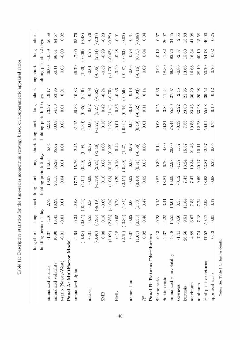
Tab
le11
:D
escr
ipti
ve
stati
stic
sfo
rth
eti
me-
seri
esm
omen
tum
stra
tegy
bas
edon
non
par
amet
ric
app
rais
alra
tios
lon
g-s
hort
lon
gsh
ort
lon
g-sh
ort
lon
gsh
ort
lon
g-sh
ort
lon
gsh
ort
lon
g-sh
ort
long
shor
t
hold
ing
per
iod
:1
day
hol
din
gp
erio
d:
5d
ays
hol
din
gp
erio
d:
10d
ays
hol
din
gp
erio
d:
22d
ays
an
nu
ali
zed
retu
rns
-1.3
7-4
.16
2.79
19.0
714
.03
5.04
32.5
413
.37
19.1
746
.00
-10.
5956
.58
an
nu
ali
zed
vola
tility
10.
9018
.43
18.9
923
.15
36.2
835
.67
33.0
854
.50
53.9
650
.11
86.6
184
.67
t-ra
tio
(New
ey-W
est)
-0.0
1-0
.01
0.01
0.04
0.01
0.01
0.05
0.01
0.01
0.05
-0.0
00.
02
Pan
el
A:
Mu
ltif
acto
rM
od
el
an
nu
ali
zed
alp
ha
-2.6
40.
34
-2.9
817
.71
15.2
62.
4531
.15
20.3
310
.83
46.7
9-7
.00
53.7
9
(-0.4
3)(0
.05)
(-0.
44)
(1.1
4)(0
.49)
(0.0
8)(1
.30)
(0.3
5)(0
.19)
(1.3
6)(-
0.06
)(0
.48)
mar
ket
-0.0
10.5
5-0
.56
-0.0
90.
28-0
.37
-0.0
60.
62-0
.68
-0.0
10.
75-0
.76
(-0.4
6)(7
.96)
(-8.
19)
(-1.
39)
(2.2
4)(-
3.48
)(-
1.27
)(5
.27)
(-6.
62)
(-0.
06)
(2.4
4)(-
2.37
)
SM
B0.
080.1
8-0
.09
0.16
0.08
0.08
0.18
0.42
-0.2
4-0
.52
-0.2
9-0
.23
(1.0
9)(2
.56)
(-1.
04)
(1.0
8)(0
.21)
(0.2
2)(1
.23)
(1.4
1)(-
0.75
)(-
1.79
)(-
0.42
)(-
0.29
)
HM
L0.1
8-0
.05
0.23
0.29
-0.1
30.
42-0
.01
0.36
-0.3
6-0
.29
-0.2
8-0
.01
(2.1
9)(-
0.3
6)(1
.81)
(2.4
5)(-
0.39
)(1
.27)
(-0.
04)
(0.6
4)(-
0.59
)(-
0.97
)(-
0.63
)(-
0.02
)
mom
entu
m0.0
70.
020.
060.
020.
09-0
.07
0.05
-0.1
30.
18-0
.03
0.28
-0.3
1
(1.6
5)(0
.33)
(1.3
3)(0
.40)
(0.8
1)(-
0.58
)(0
.49)
(-0.
62)
(0.9
3)(-
0.16
)(0
.71)
(-0.
98)
R2
0.02
0.4
80.
470.
020.
030.
050.
010.
110.
140.
020.
040.
04
Pan
el
B:
Retu
rns
Dis
trib
uti
on
Sh
arp
era
tio
-0.1
3-0
.23
0.15
0.82
0.39
0.14
0.98
0.25
0.36
0.92
-0.1
20.
67
Sor
tin
ora
tio
-2.3
7-4
.25
3.41
18.8
16.
764.
0020
.31
3.84
11.2
418
.30
-1.8
226
.07
annu
aliz
edse
miv
ola
tili
ty9.
1815
.55
13.0
116
.09
32.9
820
.00
25.4
455
.30
27.0
739
.89
92.2
634
.45
skew
nes
s-1
.41
-0.5
00.
55-0
.12
-1.5
71.
57-0
.39
-2.2
22.
45-0
.86
-2.5
72.
55
ku
rtosi
s26.
569.5
111
.84
7.43
13.2
415
.87
7.55
23.8
021
.96
13.6
615
.60
15.8
3
maxim
um
4.8
96.
677.
537.
4710
.34
21.4
610
.58
23.4
530
.20
16.6
816
.54
41.0
8
min
imu
m-7
.74
-7.1
8-7
.74
-9.6
9-2
0.17
-10.
11-1
2.28
-33.
28-2
0.98
-28.
19-4
0.10
-15.
58
%of
posi
tive
retu
rns
47.5
250.
1242
.93
48.6
353
.87
42.2
750
.94
55.0
839
.52
50.7
054
.78
40.0
0
app
rais
alra
tio
-0.1
30.
05-0
.17
0.68
0.29
0.05
0.75
0.19
0.12
0.76
-0.0
20.
25
Note
s:S
eeT
ab
le1
for
furt
her
det
ails.
48
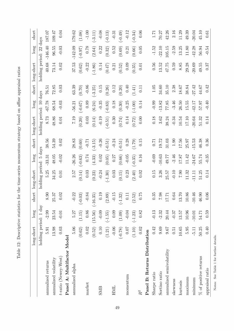
Tab
le12
:D
escr
ipti
ve
stati
stic
sfo
rth
eti
me-
seri
esm
omen
tum
stra
tegy
bas
edon
affin
eap
pra
isal
rati
os
lon
g-s
hort
lon
gsh
ort
lon
g-sh
ort
lon
gsh
ort
lon
g-sh
ort
lon
gsh
ort
lon
g-sh
ort
lon
gsh
ort
hold
ing
per
iod
:1
day
hol
din
gp
erio
d:
5d
ays
hol
din
gp
erio
d:
10d
ays
hol
din
gp
erio
d:
22d
ays
an
nu
ali
zed
retu
rns
5.9
1-2
.99
8.90
5.25
-33.
3138
.56
8.73
-67.
7876
.51
40.6
8-1
46.4
018
7.07
an
nu
ali
zed
vola
tili
ty13.
9823
.54
25.3
734
.25
48.0
554
.39
48.8
668
.54
72.8
573
.14
96.5
510
9.47
t-ra
tio
(New
ey-W
est)
0.03
-0.0
10.
020.
01-0
.02
0.02
0.01
-0.0
30.
030.
02-0
.03
0.04
Pan
el
A:
Mu
ltif
acto
rM
od
el
an
nu
ali
zed
alp
ha
5.06
5.27
-0.2
22.
57-2
6.26
28.8
37.
19-5
6.21
63.3
937
.53
-142
.09
179.
62
(0.6
2)(1
.15)
(-0.
03)
(0.1
4)(-
0.63
)(0
.60)
(0.2
0)(-
0.67
)(0
.70)
(0.6
2)(-
0.97
)(1
.08)
mar
ket
0.02
0.86
-0.8
40.
030.
74-0
.71
0.03
0.89
-0.8
6-0
.22
0.78
-1.0
0
(0.5
2)(1
5.5
6)(-
16.3
5)(0
.23)
(4.3
3)(-
3.15
)(0
.14)
(6.2
4)(-
3.25
)(-
1.86
)(2
.64)
(-3.
11)
SM
B0.
10-0
.09
0.19
-0.2
40.
02-0
.26
-0.1
9-0
.35
0.15
0.14
0.22
-0.0
8
(1.2
1)(-
1.55
)(2
.89)
(-1.
30)
(0.0
5)(-
0.51
)(-
0.51
)(-
0.83
)(0
.26)
(0.4
7)(0
.32)
(-0.
13)
HM
L-0
.06
0.09
-0.1
50.
030.
27-0
.24
0.30
0.18
0.12
0.21
0.52
-0.3
1
(-0.7
8)(1
.09)
(-1.
32)
(0.1
5)(0
.66)
(-0.
51)
(0.7
4)(0
.30)
(0.2
0)(0
.52)
(0.6
9)(-
0.49
)
mom
entu
m0.
07-0
.04
0.11
0.23
-0.0
50.
280.
14-0
.25
0.40
0.09
0.21
-0.1
2
(1.1
0)
(-1.2
3)(2
.52)
(2.4
0)(-
0.35
)(1
.79)
(0.7
2)(-
1.00
)(1
.41)
(0.3
5)(0
.66)
(-0.
34)
R2
0.02
0.82
0.75
0.02
0.16
0.15
0.00
0.14
0.11
0.01
0.05
0.06
Pan
el
B:
Retu
rns
Dis
trib
uti
on
Sh
arp
era
tio
0.42
-0.1
30.
350.
15-0
.69
0.71
0.18
-0.9
91.
050.
56-1
.52
1.71
Sor
tin
ora
tio
9.69
-2.3
27.
983.
26-1
0.63
19.7
23.
62-1
3.82
34.6
013
.52
-22.
1070
.27
annu
aliz
edse
miv
ola
tili
ty9.
6720
.44
17.7
125
.57
49.7
731
.03
38.2
477
.85
35.1
047
.75
105.
1542
.26
skew
nes
s0.
51-0
.37
0.64
-0.1
0-2
.46
1.90
-0.3
4-3
.46
2.38
0.59
-2.5
92.
16
ku
rtosi
s10.
6513.
5713
.70
7.90
17.8
717
.56
10.5
426
.50
18.6
78.
8513
.25
11.2
9
maxim
um
5.9
510.
9610
.86
11.3
211
.42
25.9
717
.10
15.5
538
.84
29.2
811
.80
49.3
9
min
imu
m-5
.11
-10.
01-1
0.46
-11.
11-2
4.67
-15.
53-2
0.64
-42.
17-2
7.42
-20.
69-4
2.28
-20.
04
%of
posi
tive
retu
rns
50.2
554.
7146
.90
51.2
555
.74
46.3
851
.32
57.9
744
.67
49.5
556
.94
45.1
0
app
rais
alra
tio
0.4
00.
590.
060.
14-0
.35
0.36
0.14
-0.4
00.
420.
37-0
.54
0.61
Note
s:S
eeT
ab
le1
for
furt
her
det
ail
s.
49