Conley index in Hilbert spaces versusthe generalized topological degree

Zbigniew Błaszczyk, Anna Gołębiewska, Sławomir Rybicki

Abstract

We prove a version of the Poincaré–Hopf theorem suitable for stronglyindefinite functionals and then apply it to infer a number of bifurcationresults in infinite-dimensional Hilbert spaces.

1 Introduction

Let H be a real Hilbert space. Fix Φ ∈ C2(H×R,R) such that ∇uΦ(0, λ) = 0

for all λ ∈ R, where ∇uΦ denotes the gradient of Φ with respect to the firstcoordinate. The purpose of this paper is to investigate non-trivial (u 6= 0)solutions of the equation

∇uΦ(u, λ) = 0, (1.1)

under sufficient regularity assumptions on Φ (see Subsection 2.1), by meansof bifurcation theory. We will be particularly interested in the existence ofconnected sets of solutions of (1.1).

In order to study bifurcation phenomena one can apply a Conley index-type theory, or a degree theory. Roughly speaking, a change of the Conleyindex implies the existence of a local bifurcation point in the set 0 × R,which amounts to the existence of a sequence of non-trivial solutions. Onthe other hand, a change of the degree implies the existence of a globalbifurcation point in the set 0 × R, i.e., the existence of a connected set ofnon-trivial solutions which satisfies the Rabinowitz alternative. (See Section4 for precise statements.) Determining when the Conley index can be usedfor detecting global bifurcation points is an interesting problem.

A classical tool for obtaining this type of results in a finite-dimensionalsetting is given by the following theorem. Below χ stands for the Eulercharacteristic of a pointed space, so that χ(S1) = −1, h for the classicalConley index, and degB for the Brouwer degree.

1

Theorem 1.1 (Poincaré–Hopf). Let Ω ⊆ Rn be an open and bounded set.Given a locally Lipschitz map Φ: Ω→ Rn, consider a flow φ such that

dφ

dt= −Φ φ, φ(0, u) = u. (1.2)

If X is an isolating neighbourhood for φ, then

χ(h(X,φ)

)= degB(Φ, IntX, 0).

We refer the reader to papers of Ćwiszewski–Kryszewski [5], McCord [14],Mrozek [15], Rybakowski [18], Srzednicki [22], Srzednicki–Wójcik–Zgliczyń-ski [23] for various versions of this result. A recent exposition together witha brief discussion of its history can be found in the paper of Styborski [24].

We provide a version of Theorem 1.1 suitable for investigating stronglyindefinite functionals. More precisely, we replace:

• χ with the Euler characteristic of a spectrum, denoted here by ,

• h with the LS-Conley index hLS of Gęba–Izydorek–Pruszko [8],

• degB with the generalized topological degree Deg, introduced indepen-dently by Guo–Liu [11] and Gołębiewska–Rybicki [10],

and obtain:

Theorem 3.10. Let H be a separable real Hilbert space. Consider a (local)flow φ satisfying (1.2) with Φ: H→ H an LS-vector field. If X is an isolatingneighbourhood for φ, then

(hLS(X,φ)

)= Deg(Φ, IntX, 0).

Then we proceed to infer a number of bifurcation theorems in infinite-dimensional Hilbert spaces.

There is a number of closely related theorems in the literature. Per-haps most urgently, Styborski [24] has an analogous result, though with adifferent notion of degree. Moreover, he is not interested in deriving bifur-cation results, which is our main goal. In the equivariant setting, there isthe second and third author paper [10], where the authors study the rela-tionship between the degree for invariant strongly indefinite functionals andthe equivariant Conley index. The present paper grew out of those consid-erations. However, the only situation considered in [10] is the case when thelinearisation of the associated operator is an isomorphism. We are able todrop this restriction in certain cases.

2

After this introduction this paper is organized in the following way. Sec-tion 2 consists of preliminaries. Perhaps most importantly, in Subsection2.1 we carefully spell out the setting we work in. In Subsections 2.2 and2.3 we review the Poincaré–Bendixson theorem and the notion of the Eulercharacteristic of a spectrum, respectively.

In Section 3 we set up and prove the aforementioned version of thePoincaré–Hopf theorem for strongly indefinite functionals. And so in Sub-section 3.1 we review the notion and properties of the LS-Conley index, andthen in Subsection 3.2 explain how to calculate it for asymptotically linearoperators in certain special cases. Subsection 3.3 contains a review of thenotion of the generalized topological degree. The Poincaré–Hopf theoremoccupies the entirety of Subsection 3.4.

The main results of Section 4 are Theorems 4.2 and 4.3, where we deriveabstract bifurcation results in infinite-dimensional Hilbert spaces.

Finally, in Section 5 we discuss examples of applications of our results tothe theory of Hamiltonian systems.

2 Preliminaries

2.1 Setting and notation

Throughout the paper H =⊕∞

k=0Hk denotes a separable real Hilbert spacewith all the subspaces Hk finite-dimensional and mutually orthogonal, andL : H→ H stands for a self-adjoint linear operator such that:

(1) H0 = kerL,

(2) L(Hk) = Hk for all k ≥ 1,

(3) 0 is isolated in the spectrum of L.

Our bifurcation results are obtained for operators Φ ∈ C2(H × R,R) ofthe following form:

Φ(u, λ) =1

2

⟨(L+ λL0)u, u

⟩H + η0(u, λ), (2.1)

where:

(S1) L0 : H → H is a linear, self-adjoint, completely and locally Lipschitzcontinuous operator, such that L0(Hk) ⊂ Hk for all k ≥ 1,

(S2) ∇uη0 : H × R → H is a completely and locally Lipschitz continuousoperator such that

∥∥∇2η0(u, ·)∥∥→ 0 as ‖u‖ → 0.

3

This choice is driven by applications: we will use operators associated withdifferential equations, especially Hamiltonian systems.

Notation. We work in the category of pointed spaces. In particular, allconsidered homotopy types are understood to be homotopy types of pointedspaces without further ado. Likewise, χ stands for the reduced Euler char-acteristic. Given a degree theory deg, we write deg(f,Ω) for deg(f,Ω, 0). Inparticular, degB is the Brouwer degree. If h is a Conley index-type theory,then h(X, f) denotes the Conley index of a (local) flow φ such that

dφ

dt= −f φ, φ(0, u) = u.

In this case we will say that the flow φ is generated by f . For r > 0, thesymbol Dr(V ), resp. Br(V ), denotes a closed, resp. open, r-neighbourhoodof 0 ∈ V .

2.2 The Poincaré–Bendixson theorem

This subsection is based entirely on the Izydorek–Rybicki–Szafraniec paper[12].

Consider the planar systemx = P (x, y)

y = Q(x, y)(2.2)

where F = (P,Q) : (R2, 0)→ (R2, 0) is an analytic vector field.Let C ⊆ R2 be a positively oriented Jordan curve of class C1 such that

F does not vanish on C and F is tangent to C only at a finite number ofpoints, say (xi, yi) ∈ C, i = 1,. . . ,k.

The solution arc(x(t), y(t)

)of (2.2) with

(x(0), y(0)

)= (x0, y0) ∈ C

is said to be internally (respectively, externally) tangent to C at (x0, y0) ifthere exists ε > 0 such that

(x(t), y(t)

)is in the interior (in the exterior)

of C for 0 < |t| ≤ ε. Write ne (respectively, nh) for the number of points(xi, yi) ∈ C for which the solution arc

(x(t), y(t)

)with

(x(0), y(0)

)= (xi, yi)

is internally (externally) tangent to C at (xi, yi).

Theorem 2.1 (Poincaré–Bendixson). Let Ω ⊆ R2 be a simply-connected,open and bounded neighbourhood of 0 ∈ R2 such that:

(1) its boundary ∂Ω is a positively oriented Jordan curve of class C1,

(2) F does not vanish on ∂Ω and is tangent to ∂Ω only at a finite numberof points,

4

(3) F has an isolated zero at 0 ∈ R2 and there are no other zeroes in Ω.

Then 2 degB(F,Ω) = 2 + ne − nh.

Since gradient operators have ne = 0, the next result is a straightforward con-sequnce of Theorem 2.1 and, in fact, a restatement of [12, Proposition 3.3].

Corollary 2.2. If F is a gradient operator and has an isolated zero at theorigin, then for r > 0 sufficiently small, Dr(R2) is an isolating block for0 ∈ R2 considered as a stationary solution of (2.2).

Moreover, let n = −degB(F,Br(R2)

). If n > −1, then the Conley index

of the origin is the homotopy type of an n-fold pointed wedge of circles.

2.3 Spectra and their Euler characteristic

Spectra. Fix a map ν : N→ N. A pair of sequences

E =(

(En)∞n=n(E), (εn)∞n=n(E)

)of pointed spaces En and maps εn : Sν(n)En → En+1, where Sν(n) denotes theν(n)-fold reduced suspension, is called a spectrum if there exists n0 ≥ n(E)

such that εn is a homotopy equivalence for all n ≥ n0.One defines notions of a map, homotopy and homotopy equivalence of

spectra in the usual manner, see e.g. [8, Section 3]. It is not difficult tosee that the homotopy type of a spectrum E depends only on the homotopytype of En for n sufficiently large.

Euler characteristic of a spectrum. Let E =((En), (εn)

)be a spectrum

with respect to a function ν : N → N. Write µn =∑n

i=0 ν(i) for any n ≥ 0.The Euler characteristic of [E] is defined by

([E])

= limn→∞

χ(Sµn−1)χ(En).

In the paper [10] Gołębiewska and Rybicki proposed the above definitionin a much broader context of G-spectra, for G being a compact Lie group(remember that χ stands for the Euler characteristic of a pointed space,hence χ(Sn)−1 = χ(Sn)). A straightforward consequence of [10, Lemma 2.3]is:

Lemma 2.3. The map is well-defined. In fact, if n0 is such that εn is ahomotopy equivalence for any n ≥ n0, then

([E])

= χ(Sµn0−1)χ(En0).

Remark 2.4. It is worth pointing out that this definition of the Euler char-acteristic coincides with the usual definition in terms of (appropriatelydefined) Betti numbers of a spectrum. See [24, Subsection 2.2] for details.

5

3 Conley index and topological degree

3.1 Conley index in Hilbert spaces

LS-vector fields. A map f : H → H is called an LS-vector field if it canbe written as

f(u) = Lu+K(u) for any u ∈ H,

where L : H→ H is as stated in Subsection 2.1, and K : H→ H is completelyand locally Lipschitz continuous. We note that LS-vector fields are usuallydefined in greater generality, with L : H → H not necessarily assumed tobe self-adjoint. We work under this additional assumption from the verybeginning in order to keep notation straighforward.

If there exist a, b > 0 such that∣∣〈K(u), u〉

∣∣ ≤ a||u||2 + b for any u ∈ H,then f is called subquadratic. We can restrict attention to subquadraticLS-vector fields without loss of generality, see [8, p. 225].

Gęba, Izydorek and Pruszko in [8] defined a Conley index for flows gen-erated by vector fields of the above form. For the sake of completeness wewill now recall their definition.

Definition of the index. Let Hn =⊕n

k=0Hk. Write Pn : H→ Hn for theorthogonal projection onto Hn, n ≥ 0. Furthermore, for any n ≥ 1 set H−nto be the L-invariant subspace of Hn corresponding to the negative part ofthe spectrum of L, and ν(n) = dimH−n+1.

Given an LS-vector field f : H→ H, define fn : Hn → Hn by setting

fn(u) = Lu+ Pn(K(u)

)for any u ∈ Hn.

Lemma 3.1 ([8, Lemma 4.1]). Let X be an isolating neighbourhood forthe flow generated by f . There exists m ∈ N such that if n ≥ m, thenXn = X ∩Hn is an isolating neighbourhood for the flow generated by fn.

It follows that Xn admits an index pair (Yn, Zn) with respect to theflow generated by fn and, consequently, h(Xn, fn) = [Yn/Zn]. Continuationproperty of Conley index implies that Sν(n)(Yn/Zn) is homotopy equivalentto Yn+1/Zn+1, hence the sequence

(En)∞n=m = (Yn/Zn)∞n=m

uniquely determines the homotopy type of a spectrum, say [E]. The LS-Conley index of X with respect to the flow generated by f , denoted byhLS(X, f), is precisely this homotopy type.

We note that the LS-Conley index enjoys the continuation property withrespect to families of LS-vector fields and abides the product formula as

6

stated below; both results are direct consequences of the relevant propertiesof the classical Conley index.

Theorem 3.2. (1) Let F : H× [0, 1]→ H be a family of LS-vector fields,i.e.

F (u, t) = Lu+K(u, t) for any u ∈ H and t ∈ [0, 1],

where K : H× [0, 1]→ H is a completely and locally Lipschitz continu-ous map. If X is an isolating neighbourhood for the flow generated byF (·, t) for each t ∈ [0, 1], then

hLS(X,F (·, 0)

)= hLS

(X,F (·, 1)

).

(2) Let fi be an LS-vector field and Xi an isolating neighbourhood forthe flow generated by fi, i = 1, 2. Then X1 × X2 is an isolatingneighbourhood for the flow generated by f1 × f2 and

hLS(X1 ×X2, f1 × f2) = hLS(X, f1) ∧ hLS(X, f2).

3.2 The Conley index of asymptotically linear operators

In the following we compute the LS-Conley index in certain special cases. Upuntil the end of this section assume that Φ ∈ C2(H×R,R) is of the form (2.1),with conditions (S1) and (S2) satisfied. In order to simplify notation, assume(without loss of generality) that λ = 1 and set Φ := Φ(·, 1), η0 := η0(·, 1).Furthermore, writeWn for the subspace of Hn corresponding to the negativepart of the spectrum of L+ L0.

Let us start with the case when L + L0 is an isomorphism, i.e. 0 /∈σ(L + L0). As an easy consequence of the continuation property and thedefinition of the index, we obtain the following fact.

Fact 3.3. If L+ L0 : H→ H is an isomorphism, then for r > 0 sufficientlysmall, Dr(H) is an isolating neighbourhood of 0 and

hLS(Dr(H),∇Φ) =[(SdimWn

)∞n=0

].

Now assume that 0 ∈ σ(L + L0). Denote V = ker(L + L0) and W =

im(L+L0). Since L+L0 is self-adjoint, H = V ⊕W . Write πV : H→ V andπW : H→W for the respective orthogonal projections and set F1 = πW ∇Φ,F2 = πV ∇Φ. Consider the following conditions:

(A1) ∇Φ(0, 0) = 0,

7

(A2) there exists p ∈ N such that di

dviF1(0, 0) and di

dviF2(0, 0) are zero for

i = 1, . . . , p, and dp+1

dvp+1F2(0, 0) is non-degenerate,

(A3) ddwF1(0, 0) is an isomorphism and d

dwF2(0, 0) = 0.

Theorem 3.4. If Φ satisfies assumptions (A1)–(A3), then 0 ∈ H is anisolated critical point of Φ.

Proof. Consider the equation ∇Φ(v, w) = 0, where v ∈ V , w ∈ W . This isequivalent to (

F1(v, w), F2(v, w))

= (0, 0). (3.1)

Concentrate on F1(v, w) = 0 first. Let ϕ : ΩV →W be given by the implicitfunction theorem in a neighbourhood ΩV of 0 ∈ V , so that the zeroes of F1

are given by(v, ϕ(v)

). Note that ϕ(0) = 0 and, in view of (A2), implicit

differentiation yields ϕ(i)(0) = 0 for i = 1, . . . , p, and, in effect, ϕ(v) =

o(‖v‖p

).

Now (v, w) is a solution of (3.1) if and only if w = ϕ(v) and F2

(v, ϕ(v)

)=

0. Denote ψ(v) = F2

(v, ϕ(v)

). Since ϕ(i)(0) = 0, we have ψ(i)(0) =

di

dviF2(0, 0) = 0 for i = 1, . . . , p. Furthermore,

ψ(p+1)(ξ) =dp+1

dvp+1F2

(ξ, ϕ(ξ)

)+

d

dwF2

(ξ, ϕ(ξ)

)ϕ(p+1)(ξ) + r(ξ),

where r(ξ) ≤ a‖ξ‖ ≤ a‖v‖ for some a > 0. Therefore r(ξ)vp+1 = o(‖v‖p+1

).

Moreover,

dp+1

dvp+1F2

(ξ, ϕ(ξ)

)vp+1 =

dp+1

dvp+1F2(0, 0)vp+1 + o

(‖v‖p+1

)and, from (A3),

d

dwF2

(ξ, ϕ(ξ)

)ϕ(p+1)(ξ)vp+1 = o

(‖v‖p+1

),

both equalities in a small enough neighbourhood. Summing up, from Taylorexpansion of ψ,

ψ(v) =ψ(p+1)(ξ)

(p+ 1)!vp+1 =

dp+1

(p+ 1)!dvp+1F2(0, 0)vp+1 + o

(‖v‖p+1

).

This in turn shows that∥∥ψ(v)∥∥ ≥ ∥∥∥∥ dp+1

dvp+1F2(0, 0)−1

∥∥∥∥−1 ‖v‖p+1 ≥ 0,

with equality if and only if v = 0. This concludes the proof.

8

Since Φ is of the form (2.1) and has zero as an isolated critical point, wecan use the so called splitting lemma (see [6, Lemma 3.2]) in order to obtaina gradient homotopy ∇H : (V ⊕W )× [0, 1]→ H which satisfies:

(H1) ∇H((v, w), 0

)= ∇Φ(v, w),

(H2) ∇H((v, w), 1

)=(∇ζ(v), A0(w)

), where ζ(v) = Φ

(v, ϕ(v)

), with ϕ

defined as in the proof of Fact 3.4, and A0 is an isomorphism given byA0 = (L+ L0)|W ,

(H3) ∇H(·, t)

=(L−∇g(·, t)

)for any t ∈ [0, 1], where ∇g is completely and

locally Lipschitz continuous, with the latter property being derived asin [6, Lemma 3.1],

(H4) ∇H−1(0)∩(Br(V )×Br(W )× [0, 1]

)= 0× [0, 1] for r > 0 sufficiently

small.

Theorem 3.5. If Φ satisfies assumptions (A1)–(A3) and 0 ∈ σ(L + L0),then

hLS(Dr(H),∇Φ) = hLS(Dr(V ),∇ζ) ∧ hLS(Dr(W ), A0)

= hLS(Dr(V ),∇vη0(·, 0)

)∧[(SdimWn

)∞n=0

].

We acknowledge that the proof of this result has been inspired by Am-brosetti’s approach in [2].

Proof. The first equality follows from the preceding discussion, continuationproperty and the product formula. Furthermore, from the definition of A0,hLS(Dr(W ), A0) =

[(SdimWn

)∞n=0

].

Consider hLS(Dr(V ),∇ζ). We will prove that ζ(v) = η0(v, 0) + o(‖v‖p

)for ‖v‖ sufficiently small. Indeed, note that

Φ(v, w) =1

2

⟨(L+ L0)(v, w), (v, w)

⟩H + η0(v, w)

=1

2

⟨(L+ L0)w,w

⟩H + η0(v, w),

hence ζ(v) = 12

⟨(L+L0)ϕ(v), ϕ(v)

⟩H+η0

(v, ϕ(v)

). Since πW

(∇Φ(v, ϕ(v))

)=

0, we have ⟨(L+ L0)ϕ(v), ϕ(v)

⟩H +

⟨∇η0

(v, ϕ(v)

), ϕ(v)

⟩H = 0

and therefore

ζ(v) = η0(v, ϕ(v)

)− 1

2

⟨∇η0

(v, ϕ(v)

), ϕ(v)

⟩H.

9

Furthermore, Taylor expansion gives

η0(v, w) = η0(v, 0) +∇wη0(v, θ · w) = η0(v, 0) + 〈∇η0(v, θ · w), w〉H,

where θ ∈ [0, 1]. But (A2) implies that∥∥∇η0(u)

∥∥ = o(‖u‖p−1

), so that∣∣⟨∇η0(v, w), w

⟩H

∣∣ ≤ a(‖v‖p−1 + ‖w‖p−1)‖w‖.

Taking w = ϕ(v) and using ϕ(v) = o(‖v‖p

), we obtain that ζ is as claimed.

Therefore, from the condition (A2) it follows that assumptions of the con-tinuation property of the Conley index are satisfied. From this property weobtain the assertion.

Let us now consider a special case of the above situation.

Remark 3.6. Assume that dimV = 2 and letm = − degB(∇η0(·, 0), Br(V )

).

Provided that m ≥ 0, from Corollary 2.2 we obtain

hLS(Dr(V ),∇vη0(·, 0)

)= [S1 ∨ · · · ∨ S1︸ ︷︷ ︸

m

].

Therefore,

hLS(Dr(V ),∇Φ) = [S1 ∨ · · · ∨ S1︸ ︷︷ ︸m

] ∧[(SdimWn

)∞n=0

]=[(SdimWn+1 ∨ · · · ∨ SdimWn+1︸ ︷︷ ︸

m

)∞n=0

].

3.3 The generalized topological degree

We retain notation of Subsections 2.1 and 3.1. In particular, f = L + K

is an LS-vector field. Furthermore, let Q : H→ H0 denote the orthogonalprojection onto H0 = kerL, and let n− denote the Morse index of the oper-ator Pn (L+Q) : Hn → Hn, i.e. its number (with multiplicity) of negativeeigenvalues.

Given an open and bounded subset Ω ⊆ H such that f−1(0) ∩ ∂Ω = ∅,we define the generalized topological degree of f as follows:

Deg(f,Ω) = limn→∞

(−1)n− degB(fn,Ω ∩Hn).

Fact 3.7. The definition above coincides with the one of degree for stronglyindefinite G-invariant functionals introduced by Gołębiewska and Rybickiin [9], provided that G is the trivial group and f is a gradient operator.

10

Proof. Note that assumptions (1) and (2) of Subsection 2.1 imply that L isa Fredholm operator of index 0, so f is in the class of functions consideredin [9].

Recall that the Gołębiewska–Rybicki degree is an element of the Eulerring

(U(G),+, ?

)given by the formula

∇G-Deg(f,Ω) = limn→∞

∇G-deg(L,B1(Hn H0)

)−1?∇G-deg(fn,Ωε ∩Hn),

where ∇G-deg stands for a degree theory introduced by Gęba [7] and Ωε is anε-neighbourhood of the set of zeroes of f . Now, if G is the trivial group, thenU(G) is isomorphic to the integers, and ∇G-deg coincides with the Brouwerdegree. Moreover, L|HnH0 is an isomorphism with the Morse index equalto the Morse index of Pn (L + Q) : Hn → Hn, and therefore its Brouwerdegree is (−1)n− . Finally, since f is defined on the entire space H, the degree∇G-deg(fn,Ω∩Hn) is well-defined and excision yields, for ε sufficiently small,

∇G-deg(fn,Ω ∩Hn) = ∇G-deg(fn,Ωε ∩Hn).

It is now clear that an argument similar to that of [9, Lemma 3.2] implies:

Lemma 3.8. The generalized topological degree Deg is well-defined: thereexists n0 such that for any n ≥ n0, the equality

Deg(f,Ω) = (−1)n− degB(fn,Ω ∩Hn)

holds.

It also follows from the Gołębiewska–Rybicki paper that Deg has manyof the usual properties expected of a degree theory, in particular existence,additivity and homotopy invariance (see [9, Theorem 3.1]).

Remark 3.9. Guo and Liu [11] introduced the notion of topological degreefor LS-vector fields as follows:

DegGL(f,Ω) = limn→∞

(−1)n− degB(fn, PnΩ).

Since the set of zeroes of f = L + K is compact, it is not difficult to seethat Deg = DegGL and we could just as well use the Guo–Liu definition. Forthe sake of simplicity of the proof of Theorem 3.10, however, it will be moreconvenient to work with intersections instead of projections.

A different approach to the definition of the degree for the LS-vectorfields is the degree relative to L, introduced, in more general setting, by

11

Mawhin in [13]. Under the assumptions of this section, we can define thisdegree by setting

degL(f,Ω) = degLS(I + L−1K,Ω),

where degLS stands for the Leray–Schauder degree, L : H → H is given byLu = Lu + Qu, and K : H → H is given by K(u) = K(u) −Qu. Using theLeray’s product formula for degLS one can show that this notion coincideswith the notion of the generalized topological degree. However note thatusing this construction, we can lose the gradient structure of the mapping.

3.4 A Poincaré–Hopf theorem for infinite-dimensional Hilbertspaces

Theorem 3.10. Let H =⊕∞

k=0Hk be a separable real Hilbert space suchthat all the subspaces Hk are finite-dimensional and mutually orthogonal. IfX is an isolating neighbourhood for the flow generated by an LS-vector fieldf : H→ H, then

(hLS(X, f)

)= Deg(f, IntX).

Proof. Assume that hLS(X, f) = [E], where E = (En)∞n=n(E). Then

(hLS(X, f)

)= χ

(Sµn′−1

)· χ(En′) for sufficiently large n′.

On the other hand,

Deg(f, IntX) = (−1)n′′− degB

(fn′′ , (IntX) ∩Hn′′

)for sufficiently large n′′.

(Recall that fn : Hn → Hn is given by fn = L+ Pn K, where Pn : H→ Hn

is the orthogonal projection.) Therefore we only need to show that

χ(Sµn0−1

)· χ(En0) = (−1)n0− degB

(fn0 , (IntX) ∩Hn0

),

where n0 = maxn′, n′′. As a preliminary step, we will prove that:

Lemma 3.11. The following statements are true for any n ≥ n0.

(1) The degree degB(fn, Int(X ∩ Hn)

)is well-defined, i.e. there are no

zeroes of the operator fn on the boundary of Int(X ∩Hn).

(2) The equality

degB(fn, (IntX) ∩Hn

)= degB

(fn, Int(X ∩Hn)

),

holds, where the interior on the right-hand side of the equation is takenwith respect to Hn.

12

Proof of Lemma 3.11. Fix n ≥ n0.Since X is compact (as it is an isolating neighbourhood), we can assume

without loss of generality that X = IntX and, consequently, ∂X = ∂ IntX.This makes it clear that if fn(x) = 0 for x ∈ X ∩Hn, then x ∈ (IntX)∩Hn.Now note that (IntX) ∩ Hn is an open subset of Int(X ∩ Hn). This provesthe first statement. The second one follows immediately from the excisionproperty of the Brouwer degree. 2

To conlude the proof of Theorem 3.10 it suffices to show that

χ(Sµn0−1

)· χ(En0) = (−1)n0− degB

(fn0 , Int(X ∩Hn0)

).

But X ∩Hn0 is an isolating neighbourhood for the flow generated by fn0 inview of Lemma 3.1, and h(X ∩Hn0 , fn0) = [En0 ] by definition of hLS , henceTheorem 1.1 yields

χ(En0) = degB(fn0 , Int(X ∩Hn0)

).

Moreover,

µn0−1 =

n0−1∑k=0

ν(k) =

n0−1∑k=0

dimH−k+1 = n0−,

and the conclusion follows.

4 Bifurcation of critical points

Fix Φ ∈ C2(H× R,R) of the form (2.1) with conditions (S1), (S2) satisfied.Assume that ∇uΦ(0, λ) = 0 for all λ ∈ R. Our aim is to investigate solutionsof the equation

∇uΦ(u, λ) = 0.

Define the set of non-trivial solutions by setting

N =

(u, λ) ∈ H× R∣∣u 6= 0 and ∇uf(u, λ) = 0

.

A solution of the form (0, λ) will be called trivial. Moreover, for λ0 ∈ Rdenote by C(λ0) ⊆ H × R a connected component of N such that (0, λ0) ∈C(λ0). A point (0, λ0) ∈ C(λ0) is called:

• a local bifurcation point if (0, λ0) ∈ N ,

• a global bifurcation point if either C(λ0) ∩(0 ×R \

(0, λ0)

)6= ∅ or

C(λ0) is unbounded.

13

In the sequel we formulate sufficient conditions for the existence of bi-furcation points. Recall that it is known that a change of the Conley index(respectively, degree) implies the existence of a local (respectively, global)bifurcation point. More precisely, we have the following result, which is aconsequence of standard properties of the index and degree, see Smoller [20]for the Conley index case and Rabinowitz [16], Zeidler [27] for the Leray–Schauder degree case.

Theorem 4.1. (1) If there exist λ1, λ2 ∈ R, λ1 < λ2, such that

hLS(Dr(H),∇uΦ(·, λ1)

)6= hLS

(Dr(H),∇uΦ(·, λ2)

),

then there exists a local bifurcation point λ ∈ (λ1, λ2).

(2) If there exist λ1, λ2 ∈ R, λ1 < λ2, such that

Deg(∇uΦ(·, λ1), Br(H)

)6= Deg

(∇uΦ(·, λ2), Br(H)

),

then there exists a global bifurcation point λ ∈ (λ1, λ2).

On the other hand, a change of the Conley index in general does not implythe existence of a global bifurcation point, see e.g. Böhme [3], Takens [26].However, under additional assumptions, using Theorem 3.10, one can showthat a change of the index implies a change of the degree, and, consequently,the existence of a global bifurcation point. In what follows we considerexamples of such phenomena.

Let us first consider the case of the isomorphism. Given λ ∈ R, writeWnλ

for the subspace of Hn corresponding to the negative part of the spectrumof L+ λL0.

Theorem 4.2. Assume that there exist λ1, λ2 ∈ R, λ1 < λ2, such that bothL+ λ1L0 and L+ λ2L0 are isomorphisms.

(1) If dimWnλ16= dimWn

λ2for n sufficiently large, then there exists a local

bifurcation point λ ∈ (λ1, λ2).

(2) If dimWnλ1− dimWn

λ2is odd for n sufficiently large, then there exists

a global bifurcation point λ ∈ (λ1, λ2).

Proof. In view of Fact 3.3, if L + λL0 is an isomorphism for some λ ∈ R,then for sufficiently small r > 0:

hLS(Dr(H),∇Φ(·, λ)

)=[SdimWn

λ].

14

Hence if dimWnλ16= dimWn

λ2, then

hLS(Dr(H),∇Φ(·, λ1)

)=[SdimWn

λ1

]6=[SdimWn

λ2

]= hLS

(Dr(H),∇Φ(·, λ2)

).

The first statement now follows immediately from Theorem 4.1 (1). As forthe second one, recall that odd- and even-dimensional spheres have differentEuler characteristics, apply to the above sequence of (in)equalities, andthen use Theorems 3.10 and 4.1 (2).

We now want to drop the condition that L + λiL0’s are isomorphisms.More precisely, we will consider the case when L+λiL0’s have two-dimensionalkernels.

Theorem 4.3. Assume that there exist λ1, λ2 ∈ R, λ1 < λ2, such that bothL + λ1L0 and L + λ2L0 have two-dimensional kernels Vλ1 and Vλ2, respec-tively. Moreover, assume that Φ(·, λ1) and Φ(·, λ2) satisfy conditions (A1)–(A3) of Subsection 3.2 and, additionally, degB

(∇η0

((·, 0), λ1

), Br(Vλ1)

)> 0,

degB(∇η0

((·, 0), λ2

), Br(Vλ2)

)> 0 for some r > 0.

(1) If dimWnλ16= dimWn

λ2for n sufficiently large, then there exists a local

bifurcation point λ ∈ (λ1, λ2).

(2) If dimWnλ1− dimWn

λ2is odd for n sufficiently large, then there exists

a global bifurcation point λ ∈ (λ1, λ2).

(3) If degB(∇vη0

((·, 0), λ1

), Br(Vλ1)

)6= degB

(∇vη0

((·, 0), λ2

), Br(Vλ2)

),

then there exists a global bifurcation point λ ∈ (λ1, λ2).

Proof. As explained in Remark 3.6, if L + λL0 has a two-dimensional ker-nel Vλ for some λ ∈ R, then

hLS(Dr(H),∇Φ(·, λ)

)=[ m∨i=1

SdimWnλ+1],

where m = −degB(∇vη0

((·, 0), λ

), Br(Vλ)

). Recall that

χ( m∨i=1

Sn)

= (−1)nm.

Now proceed in exactly the same way as in the proof of Theorem 4.2.

15

5 Applications to Hamiltonian systems

In this section we present applications of our results to Hamiltonian systems.Let us start with a brief review of a general setting of this theory. Assumethat G ∈ C2(R2m × R,R) is 2π-periodic in t and satisfies

∥∥∇G(z, t)∥∥ ≤

c1 + c2‖z‖s for (z, t) ∈ R2m×R and some c1, c2, s > 0. Consider the system

z = J∇G(z, t). (5.1)

It is known that 2π-periodic solutions of (5.1) are in one-to-one correspon-dence with critical points of the functional Φ: H→ R defined by

Φ(z) = −1

2〈Lz, z〉H − η(z),

where H = H12 (S1,R2m), 〈Lz, z〉H =

∫ 2π0 〈Jz, z〉dt, and η(z) =

∫ 2π0 G(z, t)dt.

It is known that ∇η is a completely continuous map and −∇Φ is an LS-vector field, see Gęba–Izydorek–Pruszko [8]. We refer the reader to Amann–Zehnder [1], Rabinowitz [17], or Szulkin [25] for the remaining details.

Set H±k = a cos kt± Ja sin kt | a ∈ R2m and Hk = H+k ⊕H−k . It is easy

to see that kerL = H0 and L(Hk) = Hk for all k ≥ 1. For k ≥ 0 denoteby pk : H → H the orthogonal projection onto Hk and define Λ: H → H byΛ(z) = p0(z) +

∑∞k=1

1kpk(z). From the definition of the inner product in H,

we obtain∇η(z) = Λ

(∇G(z(·), ·)

), (5.2)

and, moreover, for z = a0 +∑∞

k=1 ak cos kt+ bk sin kt,

Lz =∞∑k=1

(Jbk cos kt− Jak sin kt) (5.3)

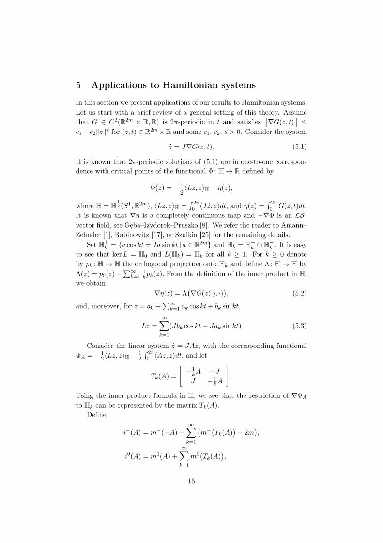
Consider the linear system z = JAz, with the corresponding functionalΦA = −1

2〈Lz, z〉H −12

∫ 2π0 〈Az, z〉dt, and let

Tk(A) =

[− 1kA −JJ − 1

kA

].

Using the inner product formula in H, we see that the restriction of ∇ΦA

to Hk can be represented by the matrix Tk(A).Define

i−(A) = m−(−A) +

∞∑k=1

(m−(Tk(A)

)− 2m

),

i0(A) = m0(A) +

∞∑k=1

m0(Tk(A)

),

16

where m−(M) denotes the Morse index of a symmetric matrix M , i.e. thenumber (with multiplicity) of negative eigenvalues of M , and m0(M) is thedimension of the kernel of M . It is easy to see that for n sufficiently large,i−(A) + n · 2m equals to the dimension of the subspace of Hn correspondingto the negative part of the spectrum of ∇ΦA. Denote this subspace by Wn.Furthermore, i0(A) is the dimension of the kernel of ∇ΦA.

If i0(A) = 0, then D(r) is an isolating neighbourhood for the isolatedinvariant set 0 of the flow induced by −∇ΦA and hLS

(D(r),∇ΦA

)= [E],

where E is a spectrum such that En = SdimWn for n sufficiently large (seeGęba–Izydorek–Pruszko [8]). On the other hand, it is known that i0(A) 6= 0

if and only if σ(JA) ∩ iZ 6= ∅. In this case

ker(∇ΦA) =

=xk sin kt+ yk cos kt, xk cos kt− yk sin kt |xk + iyk ∈ VJA(ik)

.

(5.4)

Now consider a family of Hamiltonian systems

z = J∇G(z, t, λ), (5.5)

where ∇ denotes the gradient with respect to (z, t). With this family weassociate the functional Φ : H × R → R given by Φ(z, λ) = −1

2〈Lz, z〉H −η(z, λ). The critical points (with respect to z) of this functional correspondto 2π-periodic solutions of (5.5).

Assume that

(G1) G(z, t, λ) = 12

⟨A(λ)z, z

⟩+g(z, t, λ) where A(λ) is linear and symmetric

for all λ ∈ R, and ∇g(z, t, λ) = o(‖z‖)uniformly in t and λ as z → 0.

For λ ∈ R define L0(λ) : H → H by⟨L0(λ)z, z

⟩H = −1

2

∫ 2π0

⟨A(λ)z, z

⟩dt

and put η0(z, λ) =∫ 2π0 g(z, t, λ)dt. Write Vλ for the kernel and Wλ for the

image of L+L0(λ). Let πVλ and πWλbe the orthogonal projections onto Vλ

and Wλ respectively, and define F1, F2 : H × R → H by setting F1(z, λ) =

−πWλ ∇Φ(z, λ) and F2(z, λ) = −πVλ ∇Φ(z, λ).

As an easy consequence of Theorem 4.2 we obtain following result.

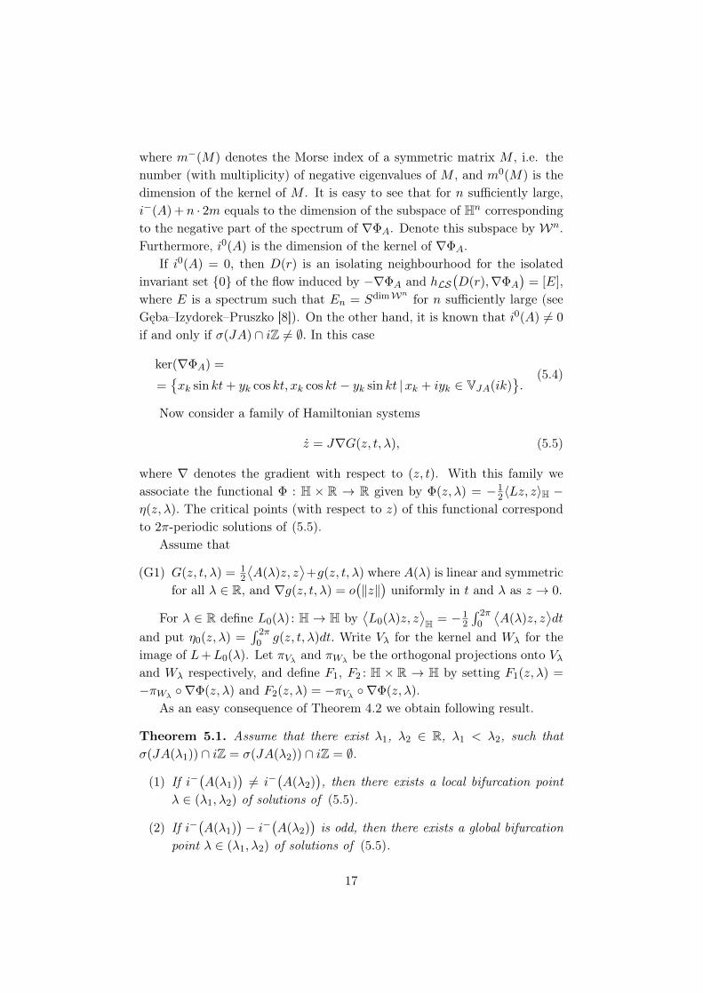
Theorem 5.1. Assume that there exist λ1, λ2 ∈ R, λ1 < λ2, such thatσ(JA(λ1)) ∩ iZ = σ(JA(λ2)) ∩ iZ = ∅.

(1) If i−(A(λ1)

)6= i−

(A(λ2)

), then there exists a local bifurcation point

λ ∈ (λ1, λ2) of solutions of (5.5).

(2) If i−(A(λ1)

)− i−

(A(λ2)

)is odd, then there exists a global bifurcation

point λ ∈ (λ1, λ2) of solutions of (5.5).

17

In the case when i0(A(λi)) 6= 0 for i = 1, 2 we have to consider additionalassumptions. In the following we work in the situation when i0

(A(λ1)

)=

i0(A(λ2)

)= 2 and use Theorem 4.3.

Theorem 5.2. Assume that there exist λ1, λ2 ∈ R, λ1 < λ2, such thati0(A(λ1)

)= i0

(A(λ2)

)= 2. Moreover, assume that Φ(·, λ1) and Φ(·, λ2) sat-

isfy conditions (A1)–(A3) of Subsection 3.2 and, additionally,degB

(∇η((·, 0), λ1

), Br(Vλ1)

)> 0, degB

(∇η((·, 0), λ2

), Br(Vλ2)

)> 0 for

some r > 0.

(1) If i−(A(λ1)

)6= i−

(A(λ2)

), then there exists a local bifurcation point

λ ∈ (λ1, λ2) of solutions of (5.5).

(2) If i−(A(λ1)

)− i−

(A(λ2)

)is odd, then there exists a global bifurcation

point λ ∈ (λ1, λ2) of solutions of (5.5).

(3) If degB(∇vη0

((·, 0), λ1

), Br(Vλ1)

)6= degB

(∇vη0

((·, 0), λ2

), Br(Vλ2)

),

then there exists a global bifurcation point λ ∈ (λ1, λ2) of solutions of(5.5).

We end this section with an example of an application of Theorem 5.2.

Example 5.3. Let us consider a family of Hamiltonian systems of the form(5.5). Assume that (G1) is satisfied and there exist λ1, λ2 such that

G(z, t, λ1) =1

2(x2 + y2) + (x4 − 6x2y2 + y4) cos(4t),

G(z, t, λ2) =1

2(x2 + y2) + (x5 − 10x3y2 + 5xy4) cos(5t).

(5.6)

We will show that in this situation the assumptions of Theorem 5.2 aresatisfied. Note that A(λ1) = A(λ2) = Id. Therefore σ

(JA(λ)

)∩ iZ = ±i

and, from (5.4),

ker(L+ L0(λ)

)= spane1 cos t+ e2 sin t, e1 sin t− e2 cos t (5.7)

for λ = λ1, λ2.Concentrate on the case λ = λ1 first. It is easy to see that d

dwF1

((0, 0), λ1

)is an isomorphism, and di

dviF1

((0, 0), λ1

)is zero for i ≥ 1. Moreover,

ddwF2

((0, 0), λ1

)is zero. We will now compute di

dviF2

((0, 0), λ1

)for i ≥ 1.

Consider F2

((v, 0), λ1

), where v ∈ Vλ1 . From (5.7) it follows that

v = a(e1 cos t+ e2 sin t) + b(e1 sin t− e2 cos t)

= (a cos t− b sin t)e1 + (a sin t+ b cos t)e2.

18

Therefore (5.3) implies that

Lv = J

[−ba

]cos t− J

[a

b

]sin t = −v. (5.8)

Moreover, from (5.2),

∇η((v, 0), λ1

)= Λ

[∇G

((((a cos t− b sin t)e1 + (a sin t+ b cos t)e2

), 0), λ1

)]= Λ

[a cos t− b sin t+ 4

(1

2a3(cos t+ cos(7t)

)− 3

2a2b(sin(7t)− sin t

)− 3

2ab2(cos t+ cos(7t)

)+b3

2

(sin(7t)− sin t

)),

a sin t+ b cos t+ 4(− a3

2

(sin(7t)− sin t

)− 3

2a2b(cos t+ cos(7t)

)+

3

2ab2(sin(7t)− sin t

)+b3

2

(cos t+ cos(7t)

))].

Summing up and using πVλ1 , we obtain

F2

((v, 0), λ1

)=[2(a3 cos t+ 3a2b sin t− 3ab2 cos t− b3 sin t),

2(a3 sin t+ 3a2b cos t− 3ab2 sin t+ b3 cos t)]

= 2(a3 − 3ab2)

[cos t

sin t

]+ 2(−3a2b+ b3)

[− sin t

cos t

],

or, equivalently,

F2

((a, b, 0), λ1

)=(2(a3 − 3ab2), 2(−3a2b+ b3)

).

Hence the first non-vanishing derivative of F2

((0, 0), λ1

)is nondegenerate

and (A1)–(A3) of Subsection 3.2 are satisfied. Moreover, since v ∈ Vλ1 ,

∇vη0((·, 0), λ1) = F2((·, 0), λ1).

In the same way we can consider the case λ = λ2 and obtain

F2

((a, b, 0), λ2

)=(5

2(a4 − 6a2b2 + b4),

5

2(−4a3b+ 4ab3)

).

Hence, from the above computations we obtain that condition (3) of Theorem5.2 is satisfied. Therefore there exists a global bifurcation point λ ∈ (λ1, λ2)

of solutions of the system in question.

Acknowledgements. The authors have been supported by the NationalScience Centre under grant 2012/05/B/ST1/02165.

19

References

[1] H. Amann, E. Zehnder, Periodic solutions of asymptotically linear Hamiltoniansystems, Manuscripta Math. 32 (1980), 149–189.

[2] A. Ambrosetti, Branching points for a class of variational operators, J. Anal.Math. 76 (1998), 321–335.

[3] - R. Böhme, Die Lösung der Verzweigungsgleichungen für nichtlineareEigenwert-probleme, Math. Z. 127 (1972), 105–126.

[4] R. F. Brown, A topological introduction to nonlinear analysis, Birkhauser, 2004.

[5] A. Ćwiszewski, W. Kryszewski, On a generalized Poinacaré–Hopf formula ininfinite dimensions, Discrete Contin. Dyn. Syst. 29 (2011), 953–978.

[6] J. Fura, A. Ratajczak, S. Rybicki, Existence and continuation of periodic solu-tions of autonomous Newtonian systems, J. Diff. Eq. 218 (2005), 216–252.

[7] K. Gęba, Degree for gradient equivariant maps and equivariant Conley index,Topological Nonlinear Analysis II, Birkhäuser, 1997, 247–272.

[8] K. Gęba, M. Izydorek, A. Pruszko, The Conley index in Hilbert spaces and itsapplications, Studia Math. 134 (1999), 217–233.

[9] A. Gołębiewska, S. Rybicki, Global bifurcations of critical orbits of G-invariantstrongly indefinite functionals, Nonlinear Anal. 74 (2011), 1823–1834.

[10] A. Gołębiewska, S. Rybicki, Equivariant Conley index versus degree for equiv-ariant gradient maps, Discrete Contin. Dyn. Syst. Ser. S 6 (2013), 985–997.

[11] Y. Guo, J. Liu, Bifurcation for strongly indefinite functional and applicationsto Hamiltonian system and noncooperative elliptic system, J. Math. Anal. Appl.359 (2009), 28–38.

[12] M. Izydorek, S. Rybicki, Z. Szafraniec, A note on the Poincaré–Bendixsonindex theorem, Kodai Math. J. 19 (1996), 145–156.

[13] J. Mawhin, Topological degree methods in nonlinear boundary value problems,CBMS Regional Conference Series in Mathematics 40, AMS, 1979.

[14] C. K. McCord, On the Hopf index and the Conley index, Trans. Amer. Math.Soc. 313 (1989), 853–860.

[15] M. Mrozek, The fixed point index of a translation operator of a semiflow, Univ.Iagel. Acta Math. 27 (1988), 13–22.

[16] P. H. Rabinowitz, Some global results for nonlinear eigenvalue problems, J.Func. Anal. 7 (1971), 487–513.

[17] P. H. Rabinowitz, Minimax methods in critical point theory with applicationsto differential equations, CBMS Regional Conference Series in Mathematics 65,AMS, 1986.

20

[18] K. Rybakowski, On a relation between the Brouwer degree and the Conleyindex for gradient flows, Bull. Belg. Math. Soc. Simon Stevin 37 (1985), 87–96.

[19] K. Rybakowski, The homotopy index and partial differential equations,Springer-Verlag, 1987.

[20] J. Smoller, Shock waves and reaction-diffusion equations, Springer-Verlag,1994.

[21] J. Smoller, A. Wasserman, Bifurcation and symmetry-breaking, Invent. Math.100 (1990), 63–95.

[22] R. Srzednicki, On rest points of dynamical systems, Fund. Math. 126 (1985),69–81.

[23] R. Srzednicki, K. Wójcik, P. Zgliczyński, Fixed point results based on theWażewski method, Handbook of Topological Fixed Point Theory, Springer, 2005,905–943.

[24] M. Styborski, Conley index in Hilbert spaces and the Leray–Schauder degree,Topol. Methods Nonlinear Anal. 33 (2009), 131–148.

[25] A. Szulkin, Cohomology and Morse theory for strongly indefinite functionals,Math. Z. 209 (1992), 375–418.

[26] F. Takens, Some remarks on the Böhme–Berger bifurcation theorem, Math. Z.129 (1972), 359–364.

[27] E. Zeidler, Nonlinear functional analysis and its applications I: Fixed-pointtheorems, Springer, 1986.

Zbigniew BłaszczykFaculty of Mathematics and Computer ScienceNicolaus Copernicus UniversityChopina 12/1887-100 Toruń, Polandblaszczyk@mat.umk.pl

Anna GołębiewskaFaculty of Mathematics and Computer ScienceNicolaus Copernicus UniversityChopina 12/1887-100 Toruń, Polandanna.golebiewska@mat.umk.pl

Sławomir RybickiFaculty of Mathematics and Computer ScienceNicolaus Copernicus UniversityChopina 12/1887-100 Toruń, Polandrybicki@mat.umk.pl

21