Embed Size (px)
Citation preview

Connectionist Taxonomy Learning
Inaugural-Dissertation
zur
Erlangung der Doktorwürde
der
Philosophischen Fakultät
der
Rheinischen Friedrich-Wilhelms-Universität
zu Bonn
vorgelegt von
Miłosław L. Frey
aus Kraków
Bonn, 2007
Gedruckt mit der Genehmigung der Philosophischen Fakultät
der Rheinischen Friedrich-Wilhelms-Universität Bonn
Zusammensetzung der Prüfungskommision
Herr PD Dr. Bernhard Schröder
(Vorsitzender)
Herr Prof. Dr. Winfried Lenders
(Betreuer und Gutachter)
Herr PD Dr. Ulrich Schade
(Gutachter)
Herr Prof. Dr. Wolfgang Hess
(weiteres prüfungsberechtigtes Mitglied)
Tag der mündlichen Prüfung: 3. Mai 2007
Diese Dissertation ist auf dem Hochschulschriftenserver der ULB Bonn
http://hss.ulb.uni-bonn.de/diss_online elektronisch publiziert
Miłosław L. Frey
Connectionist Taxonomy Learning


I don’t want knowledge, I want certainty
I don’t want knowledge, I want certainty
Oh I get a little bit afraid
Sometimes
David Bowie
Law (Earthlings on Fire), 1997


Introduction
Categorization is one of the most common phenomena one has
to deal with during one’s lifetime. Whatever action we have to
take, the categorization is a preassumption. Categorization is not
only connected to sensual experiences, like, for example, perceiv-
ing colors or sounds, but also deals with our activities. Moreover,
each mental system human is able to create, has a notion of cate-
gorization. In linguistics, for example, categories emerge on each
language level: from phonetics to pragmatics. Categorization is
thus fundamental in all kinds of interaction with the world.
Although categorization is so important to us, it is one of
the least known and least understood processes. It has been a
long time since scientists started to investigate the categorization
1

process and to model it — in my opinion still without really con-
vincing results.
With this work I would like to contribute to the investigation
of categorization. I am far from stating that my model is the best,
or even better than what was already done. However, I would like
to present it as an anchor point for further investigations, because
I believe that my ideas contain some potential to challenge several
current problems in cognitive sciences.
The tool used to implement my model is based on a connec-
tionist paradigm. However, I would not like to contribute to the
eternal opposition between localist versus distributed branches of
connectionism. In my opinion, there is no “black or white”. In-
stead, there is no possibility to use either pure localist or pure
distributed formalism in more complex systems (even if their in-
ventors state so). That is why my model tries to incorporate
aspects of both flavors of connectionism.
The model of categorization presented here is of course not
the ultimate way to describe this process. In the present stage it
focuses on the creation of the hierarchy (taxonomy) of concepts
in an easily readable way. I would not like to state that it is able
to model real cognitive processes. Instead my aim was to create a
formal but usable way to describe them. I hope that it can help in
understanding them and at the same time it will create a frame-
work for applications. The most obvious is automatic classification
of different items, and thus supporting the lexicon creation within
2

more sophisticated computer-linguistic applications. As a further
application, my model can serve as a base to create full (or at
least more developed) ontologies in different domains of computer
and language sciences.
3

Outline
This work is divided as follows. The first part deals with theoret-
ical issues. In Chapter 1 the terms category, categorization and
taxonomy are introduced in the context of this work. Further,
categorization models proposed in the literature (Chapter 2) as
well as basics of connectionism (Chapter 3) are described. The
second part goes into details of the model proposed here. Chapter
4 explicates the architecture of a single node as well as of the whole
network, followed by Chapter 5 that presents details of the imple-
mentation of the model. The following Chapter 6 presents several
experiments conducted with the use of the model in question and
compares the results against real psychological experimental data.
Chapter 7 summarizes the description of the model itself, whereas
Chapter 8 closes this work with conclusions. Additionally, two
5

appendices (Appendix A and B) present central elements of Java
and dot source code as implemented in order to evaluate the model
presented.
6

Contents
I Theory 19
1 Categories, Categorization and Taxonomies 21
1.1 Category . . . . . . . . . . . . . . . . . . . . . . . . 22
1.1.1 Aristotle . . . . . . . . . . . . . . . . . . . . 22
1.1.2 Immanuel Kant . . . . . . . . . . . . . . . . 23
1.1.3 Category in this work . . . . . . . . . . . . 24
1.2 Where do categories come from? . . . . . . . . . . 26
1.3 Taxonomies . . . . . . . . . . . . . . . . . . . . . . 26
2 Models of Categorization 29
2.1 The Classical Model . . . . . . . . . . . . . . . . . 32
2.1.1 Feature Model in Phonology . . . . . . . . . 33
7

2.1.2 Feature Model in Other Linguistic Fields . . 34
2.1.3 Feature Model and Language Acquisition . 37
2.2 Non-Classical Models . . . . . . . . . . . . . . . . . 38
2.2.1 Rosch’s “Standard” Prototype Model . . . . 40
2.2.2 Family Resemblance . . . . . . . . . . . . . 53
2.2.3 Exemplar-Based Model . . . . . . . . . . . 57
2.3 No Clear-Cut Between Models . . . . . . . . . . . . 58
2.4 Learning Categories . . . . . . . . . . . . . . . . . 59
3 Connectionism 63
3.1 On the History of Connectionism . . . . . . . . . . 65
3.2 Algorithmic Model Theory . . . . . . . . . . . . . . 68
3.3 Remarks on Data Representation . . . . . . . . . . 69
3.3.1 Localist Data Representation . . . . . . . . 70
3.3.2 Distributed Data Representation . . . . . . 71
3.3.3 Meaning of a Unit . . . . . . . . . . . . . . 71
3.3.4 Semantic Problems . . . . . . . . . . . . . . 72
3.4 Distributed Connectionism . . . . . . . . . . . . . . 73
3.4.1 The Artificial “Neuron” . . . . . . . . . . . 74
3.4.2 Basic Architecture . . . . . . . . . . . . . . 77
3.4.3 Learning . . . . . . . . . . . . . . . . . . . . 78
3.4.4 Self-Organizing Maps . . . . . . . . . . . . . 81
3.5 Localist Connectionism . . . . . . . . . . . . . . . . 85
3.5.1 Theory of Retrieval in Sentence Production 86
8
3.5.2 Spreading Activation and Language Produc-
tion . . . . . . . . . . . . . . . . . . . . . . 87
3.5.3 Aphasia Model . . . . . . . . . . . . . . . . 88
3.5.4 Connectionist Speech Production . . . . . . 89
3.6 Semantic Networks . . . . . . . . . . . . . . . . . . 89
3.6.1 Concepts . . . . . . . . . . . . . . . . . . . 90
3.6.2 Semantic Network . . . . . . . . . . . . . . 92
3.7 Connectionism vs. Brain Structure . . . . . . . . . 102
3.8 Connectionism and Language Processing . . . . . . 104
3.9 My Categorization Model and Connectionism . . . 105
II Practice 107
4 Architecture and Operation of the Model 109
4.1 A Node . . . . . . . . . . . . . . . . . . . . . . . . 110
4.2 Activation Spreading . . . . . . . . . . . . . . . . . 113
4.2.1 Signals from Parent Nodes. . . . . . . . . . 113
4.2.2 Signals from Child Nodes . . . . . . . . . . 120
4.2.3 Final Activation Function . . . . . . . . . . 120
4.2.4 Implementation . . . . . . . . . . . . . . . . 122
4.3 Connections . . . . . . . . . . . . . . . . . . . . . . 122
4.4 Learning . . . . . . . . . . . . . . . . . . . . . . . . 123
4.4.1 Concept Learning . . . . . . . . . . . . . . . 126
4.4.2 Introspective Processes . . . . . . . . . . . . 128
9

5 Implementation 131
5.1 Objectives . . . . . . . . . . . . . . . . . . . . . . . 131
5.2 Realization . . . . . . . . . . . . . . . . . . . . . . 132
5.2.1 Nodes . . . . . . . . . . . . . . . . . . . . . 133
5.2.2 Network . . . . . . . . . . . . . . . . . . . . 134
5.2.3 Network visualization . . . . . . . . . . . . 134
5.3 Summary . . . . . . . . . . . . . . . . . . . . . . . 135
6 Evaluation 137
6.1 Introductory Simulation: Creating a Taxonomy . . 139
6.1.1 Training Data . . . . . . . . . . . . . . . . . 139
6.1.2 Storing the Data . . . . . . . . . . . . . . . 140
6.1.3 Creating a Hierarchy . . . . . . . . . . . . . 142
6.1.4 Network Pruning . . . . . . . . . . . . . . . 144
6.1.5 Discovery . . . . . . . . . . . . . . . . . . . 145
6.1.6 Final Network . . . . . . . . . . . . . . . . . 148
6.1.7 Summary . . . . . . . . . . . . . . . . . . . 149
6.2 Introductory Simulation: Autoassociation . . . . . 150
6.2.1 Preparing a Network . . . . . . . . . . . . . 150
6.2.2 Autoassociation Process . . . . . . . . . . . 151
6.3 Introductory Simulation: Generalization . . . . . . 154
6.4 Cup or Bowl: Fuzzy Categorization . . . . . . . . . 157
6.4.1 Original Experiment . . . . . . . . . . . . . 160
6.4.2 Simulation . . . . . . . . . . . . . . . . . . . 162
6.5 Cats Could Be Dogs . . . . . . . . . . . . . . . . . 169
10

6.5.1 Original Experiment . . . . . . . . . . . . . 169
6.5.2 Simulation . . . . . . . . . . . . . . . . . . . 170
7 Model Properties 177
7.1 Description Autocompletion and Noise Reduction . 177
7.2 Generalization . . . . . . . . . . . . . . . . . . . . . 178
7.2.1 Overfitting . . . . . . . . . . . . . . . . . . 179
7.3 Family Resemblance . . . . . . . . . . . . . . . . . 180
7.4 Fuzzy Categorization . . . . . . . . . . . . . . . . . 181
7.5 Priming . . . . . . . . . . . . . . . . . . . . . . . . 182
7.6 Lexical Items . . . . . . . . . . . . . . . . . . . . . 183
7.7 Asymmetric Category Learning . . . . . . . . . . . 184
7.8 Localism and Distributionism . . . . . . . . . . . . 185
7.8.1 Comparison against PDP-networks . . . . . 187
7.9 Biological Inspiration . . . . . . . . . . . . . . . . . 188
8 Conclusions 191
Bibliography 195
A Implementation of the Central Algorithm Parts 223
A.1 Activation from Parent Nodes . . . . . . . . . . . . 223
A.2 Activation from Child Nodes . . . . . . . . . . . . 224
A.3 Final Activation . . . . . . . . . . . . . . . . . . . . 225
B Example dot description of a network 227
11


List of Figures
2.1 Clark’s hierarchical features setup. . . . . . . . . . 37
2.2 Two axes of categorization. . . . . . . . . . . . . . 42
2.3 Farmers’ classification of leaf feeding insects in Leyte,
Philippines . . . . . . . . . . . . . . . . . . . . . . 46
2.4 The radial structure of category. . . . . . . . . . . 54
2.5 The non-radial structure of category. . . . . . . . . 55
3.1 Hierarchy of different cognitive models. . . . . . . . 65
3.2 Rosenblatt’s perceptron. . . . . . . . . . . . . . . . 66
3.3 Local and distributed data representation. . . . . . 70
3.4 An artificial neuron. . . . . . . . . . . . . . . . . . 75
3.5 Sigmoidal (standard logistic) function. . . . . . . . 76
3.6 Multi-layer perceptron schema. . . . . . . . . . . . 78
13

3.7 WebSOM example. . . . . . . . . . . . . . . . . . . 83
3.8 An example of a dendrogram . . . . . . . . . . . . 84
3.9 The meaning triangle. . . . . . . . . . . . . . . . . 91
3.10 Tree of Porphyry. . . . . . . . . . . . . . . . . . . . 95
3.11 A sophisticated semantic network . . . . . . . . . . 97
3.12 Hierarchical semantic memory model by Collins
and Quillian (1969). . . . . . . . . . . . . . . . . . 98
3.13 Spreading activation network in the tradition of
Collins and Loftus (from Collins and Loftus, 1975,
p. 412). . . . . . . . . . . . . . . . . . . . . . . . . 99
3.14 A propositional network representing a structure
on the sentence level. . . . . . . . . . . . . . . . . . 100
3.15 A simple KL-ONE network of generic concepts (from
Brachman and Schmolze, 1985, p. 180). . . . . . . 101
3.16 A network representing a sentence in KL-ONE (from
Brachman and Schmolze, 1985, p. 214). . . . . . . 102
3.17 A neuron . . . . . . . . . . . . . . . . . . . . . . . 103
4.1 Internal structure of a node. . . . . . . . . . . . . . 112
4.2 Two sample nodes in 2D phase space. . . . . . . . . 114
4.3 Example Gaussian functions . . . . . . . . . . . . . 118
5.1 Class diagram. Only the most relevant fields and
methods are shown. . . . . . . . . . . . . . . . . . . 136
6.1 Raw input data presented as a network structure. . 143
6.2 The incorrect class—superclass connection . . . . . 144
14
6.3 Detecting incorrect class—superclass connection . . 146
6.4 The form of a network after the discovery procedure. 148
6.5 The final form of a network: the taxonomical struc-
ture. . . . . . . . . . . . . . . . . . . . . . . . . . . 149
6.6a Starting network for autoassociation demonstration. 152
6.6b First step of autoassociation: activating some nodes. 155
6.6c Successful autoassociation . . . . . . . . . . . . . . 156
6.7a Starting point for generalization process. . . . . . . 158
6.7b Successful autoassociation in case of contradicting
features. . . . . . . . . . . . . . . . . . . . . . . . . 159
6.8 Drawings used for simulation of Labov’s experiment. 162
6.9 Results of simulation of Labov’s experiment (neu-
tral context). . . . . . . . . . . . . . . . . . . . . . 166
6.10 Results of simulation of Labov’s experiment (food
context). . . . . . . . . . . . . . . . . . . . . . . . . 167
6.11 Original figure from Labov (1974). . . . . . . . . . 168
6.12 Result of “cats and dogs” experiment. . . . . . . . . 175
15

List of Tables
2.1 Different prototypical objects. . . . . . . . . . . . . 53
6.1 Data for introductory simulation. . . . . . . . . . . 141
6.2 Data for autoassociation simulation. . . . . . . . . 151
6.3 Data used for simulation of Labov’s experiment. . . 163
6.4 Results of simulation of Labov’s experiment (neu-
tral context). . . . . . . . . . . . . . . . . . . . . . 166
6.5 Results of simulation of Labov’s experiment (food
context). . . . . . . . . . . . . . . . . . . . . . . . . 167
6.6 Data for cats in “cats and dogs” experiment. . . . . 171
6.7 Data for dogs in “cats and dogs” experiment. . . . 172
17


Part I
Theory

CHAPTER 1
Categories, Categorization and Taxonomies
Categories and categorization are one of the most important con-
cepts in one’s life. Usage of categories is usually not noticed, but
precedes many other activities. Categorization is a process which
prepares people to take any action by assigning received signals
and actions to be performed to different sets of equivalent enti-
ties. Thanks to this process, it is possible to store and manage
an infinite number of stimuli and possible actions taking place in
the real world. Although everybody has a feeling of what cate-
gory and categorization mean, the exact meanings of these terms
are discussable and are indeed defined differently by different au-
thors (cf. below). Therefore, this chapter briefly introduces the
21

22 CATEGORIES, CATEGORIZATION AND TAXONOMIES
meaning of these terms as used further in this work.
1.1 Category
The term category comes from the Greek word κατηγoρια which
means “assertion” or “accusation”. In the following, I present some
views on categories and category systems. They can be regarded
as milestones on the way to understanding a category, as used in
this work.
1.1.1 Aristotle
The first systematic work on categories is the Aristotelian text
“Categories” (Aristotle, 1928). Aristotle begins with the definition
of equivocality, univocality and derivativeness. These three terms
are then used to describe relations between objects and thereby
also their belonging to a given group of objects.
According to Aristotle, each atomic thing (that means a thing
without a further internal structure) or a living being can be at-
tributed one of ten characteristics: substance, quantity, quality,
relation, action, affection, place, time, position or state. In Aris-
totle’s view these characteristics are inherent.
“To sketch my meaning roughly, examples of substance
are ‘man’ or ‘the horse’, of quantity, such terms as
‘two cubits long’ or ‘three cubits long’, of quality, such
attributes as ‘white’, ‘grammatical’. ‘Double’, ‘half’,
Category 23
‘greater’, fall under the category of relation; ‘in a mar-
ket place’, ‘in the Lyceum’, under that of place; ‘yes-
terday’, ‘last year’, under that of time. ‘Lying’, ‘sit-
ting’, are terms indicating position, ‘shod’, ‘armed’,
state; ‘to lance’, ‘to cauterize’, action; ‘to be lanced’,
‘to be cauterized’, affection.” (Categories, Chap. 4
Aristotle, 1928)
These attributes define ten main categories for every item in
the world: a system of categories which forms a list of the highest
genera of things. A complete system of categories in the Aris-
totelian spirit would offer a systematic inventory of everything
that exists, considered at the most abstract level.
1.1.2 Immanuel Kant
Skepticism about the ability to extract inherent properties of ob-
jects, thus defining intrinsic divisions of reality, led to the next
step in understanding categories which was made by Kant in his
“Kritik der reinen Vernunft” (Kant, 1787/1990). He denied this
ability to access the internal world’s structure but believed that
one can discover our categories of understanding. Thus, the main
question he tried to answer in the abovementioned work was how
much can experience support understanding. Obviously, to an-
swer this question one has to discover the fundamental types of
subjective understanding which organize perceptions into knowl-
edge.

24 CATEGORIES, CATEGORIZATION AND TAXONOMIES
“Wenn wir von allem Inhalte eines Urteils überhaupt
abstrahieren, und nur auf die bloße Verstandesform
darin achtgeben, so finden wir, daß die Funktion des
Denkens in demselben unter vier Titel gebracht wer-
den können, deren jeder drei Momente unter sich ent-
hält. Sie können füglich in folgender Tafel vorgestellt
werden.
1. Quantität der Urteile: Allgemeine; Besondere;
Einzelne
2. Qualität: Bejahende; Verneinende; Unendliche
3. Relation: Kategorische; Hypothetische; Disjunk-
tive
4. Modalität: Problematische; Assertorische; Apodik-
tische”
(Kant, 1787/1990, §9)
These twelve modes define concepts of understanding which
Kant calls “categories” (1787/1990, §10). For Kant, the categories
are a priori and transcendental. They are used for making judg-
ments which constitute preconditions for principles of understand-
ing nature.
1.1.3 Category in this work
For the purpose of this work, a category is defined in a simple
way which summarizes the common components of Aristotle’s and

Category 25
Kant’s category systems, and simultaneously agrees with the com-
mon understanding of this term. Category is defined here as an
imaginary container, that contains all objects which are similar
to each other and simultaneously different to objects from other
categories (containers).
However, unlike in most philosophers’ works, the number and
type of categories or characteristics which lead to assigning a cat-
egory cannot be defined, because the goal of the investigations
presented here is not to find a unique answer to the ontological
question of what kinds of universal genera exist. Thus, the num-
ber of categories in the system presented here is neither defined
nor limited. It also means that categories are not given a priori
but emerge from experience.
One must note that there are several ways to “measure” the
similarity of objects. These methods actually define the models
of categorization. Aristotle and Kant used intrinsic properties of
objects or modes of understanding to assign any item into one cat-
egory. The way to measure the similarity which I use in the system
presented here is also based on properties (here also referred to
as features), but these features are treated in a more flexible way,
and – even more important – they can be graded and may contain
intermediate states. The most important models of categoriza-
tion which developed from the Aristotelian yes/no method to the
modern psychologically based ones are described in the following
chapter 2.

26 CATEGORIES, CATEGORIZATION AND TAXONOMIES
1.2 Where do categories come from?
Categories are not completely arbitrary. One can find many clues
in the world that give the basis for categorization.
The world is structured because real–world attributes
do not occur independently of each other. (. . . ) That
is, combinations of attributes of real objects do not
occur uniformly. Some pairs, triples, or ntuples are
quite probable, appearing in combination sometimes
with one, sometimes with another attribute; others
are rare; others logically cannot or empirically do not
occur. (Rosch et al., 1976)
This means that not only the pure characteristic of a given object
is necessary. The most important thing is the cooccurence of
properties. As a consequence, the analysis of clusters of features
can lead to the discovery of a category.
A process of categorization does not only mean finding simi-
larities between instances of the given class. It is also searching
for differences to instances of other classes. Those differences help
in creating characteristics of a given category.
1.3 Taxonomies
Categorization, that is, finding categories in unstructured data,
is here regarded as a synonym of classification. The classification

Taxonomies 27
in hierarchical systems is building a taxonomy (from greek ταξoζ
“arrangement, order” and -νoµια “method”). Thus a taxonomy is
a method of arrangement or a method of ordering.
Taxonomies are hierarchical arrangements of objects (things,
concepts etc.) displaying usually parent-child relationships. The
parent-child relationship, also referred to as is-a or subsumption
relationship, is in the main scope of this work. Hierarchical tax-
onomies are tree structures with a single root node (top node)
that applies to all objects in the hierarchy.
The aim of the work presented here is the construction and
evaluation of a system that creates a taxonomical tree structure
emerging from the previously unstructured input data and there-
fore performs categorization automatically. The system consists
of logical nodes which are analogue to taxonomical units and con-
nections which define the relations between nodes. In the course
of operation, this system of nodes organizes itself into a taxonom-
ical tree structure – the hierarchy – which reproduce the relations
between objects represented by the nodes.


CHAPTER 2
Models of Categorization
Categorization is one of the most important cognitive processes.
“There is nothing more basic than categorization to
our thought, perception, action, and speech. Every
time we see something as a kind of thing, (. . . ) we
are categorizing. Whenever we reason about kinds of
things (. . . ) we are employing categories. Whenever
we intentionally perform any kind of action, (. . . ) we
are using categories.” (Lakoff, 1987, p. 5)
Categorization creates a framework for the interpretation of
experiences. Its goal is to group individual entities by neglecting
29

30 MODELS OF CATEGORIZATION
subtle differences in individual experiences when they are not nec-
essary. Without categorization the world would seem constantly
changing and thus probably impossible to explore (cf. Smith and
Medin, 1981). It is important to realize that although categoriza-
tion is usually performed unconsciously and without noticeable
effort it is nevertheless a process which has to be learned. Even
more, the categories themselves are not innate and must be ac-
quired from experience.
Especially in linguistics – in phonology, in morphology and
syntax as well as in semantics – categorization is a process of high
value. In linguistics, categorization is used at two levels (Taylor,
2001): to describe the subject of its exploration and also to in-
terrelate linguistic terms to the real world. Language components
can be classified not only according to their formal structure or
membership in specific groups of grammatical entities but also as
labels for phenomena encountered in real world. For example, the
term red is not only an instantiation of the word class “adjective”
but also denotes a bundle of visual experiences.
Labov (1974) points out that this preferential reputation of
categorization often moves away from scope the understanding of
the nature of categories:
“The categorization is such a fundamental part of lin-
guistic activity that the properties of categories are
normally assumed rather than studied.” (p. 342)

31
As an interesting example of the above statement, one can
quote the Whorf’s principle of linguistic determinism (cf. Gipper,
1972). Whorf assumed that categories used by people are given
along with the language they use, and as such, they split the world
according to the concepts expressed by a language.
“We dissect nature along lines laid down by our native
languages. The categories and types that we isolate
from the world of phenomena we do not find there be-
cause they stare every observer in the face; on the con-
trary, the world is presented in a kaleidoscopic flux of
impressions which has to be organized by our minds –
and this means largely by the linguistic systems in our
minds. We cut nature up, organize it into concepts,
and ascribe significances as we do, largely because we
are parties to an agreement to organize it in this way –
an agreement that holds throughout our speech com-
munity and is codified in the patterns of our language.
(. . . ) All observers are not led by the same physical ev-
idence to the same picture of the universe, unless their
linguistic backgrounds are similar, or can in some way
be calibrated.” (Whorf, 1956, p. 213-214)
However, to understand the linguistic as well as psychological
processes of categorization it is important to know what a cat-
egory is and how it can be defined. Moreover, the discovery of
a structure of categories and dependencies between them is also
32 MODELS OF CATEGORIZATION
significant. To tackle these problems there has to exist a model of
categorization and categories.
This chapter presents an overview over different models of cat-
egorization. It starts with the classical one which formed a base
for language analysis in the twentieth century. In contrast to this
view, models based on new psychological and linguistic findings
have arisen. The prototype and exemplar based models, to name
the most prominent ones, are described here to illustrate efforts
to overcome the limitations of the classical model.
2.1 The Classical Model
The classical view on categorization has its origin in works of
Aristotle (1928, 1908). Aristotle defines the category membership
on the base of the following assumptions.
• Categories are defined by a set of necessary and jointly suf-
ficient rules based on features.
• Features have binary nature. This means they may be ei-
ther present or not. This is a consequence of a rule that
something has either to exist or not, and everything either
posses a certain feature or not.
• Thus categories have well defined and sharp borders and are
disjunctive. There are no objects which belong partially to
some category or which belong to more than one category.
The Classical Model 33
• All elements of categories are equally good because they are
defined by the same set of binary features, shared by all
members.
The Aristotelian way of defining categories strongly influenced
the linguistics of the twentieth century. It forms a base for many
theories in phonology as well as in syntax and semantics.
2.1.1 Feature Model in Phonology
Probably the most spectacular success the classical view cele-
brated, was with respect to phonology, which defines speech as a
set of phonemes. Phonemes are described by a set of features. Ac-
cording to Chomsky and Halle (1968) the binary nature of phono-
logical features is important because they are used for classifica-
tion. Using the “yes/no mechanism” is a natural method to show
whether a unit in question is a member of a given category or not.
The noteworthy success of Aristotelian feature-based mech-
anism inclined many phonologists to develop it further, and to
enrich the properties of phonological features by additional as-
sumptions:
• Features are primitive, i.e., they have no internal structure
and cannot be decomposed further.
• Features are universal. All phoneme classes are defined by a
set of features common to all languages which express human
articulation ability.

34 MODELS OF CATEGORIZATION
• Features are abstract. They do not describe directly any
physical phenomena related to speech production or com-
prehension but they appear only as a classificatory markers
(in contrast to the phonetic features that range over a full
scale of physical phenomena, cf. Chomsky and Halle, 1968,
chapter 7).
• Sometimes it is also postulated that phonological features
are innate. This is a consequence of the two latter char-
acteristics: if they are really universal and abstract, they
cannot be acquired from physical data, so there is no possi-
bility for children to learn them. Thus, they must be innate.
2.1.2 Feature Model in Other Linguistic Fields
A classification theory based on the assumptions listed above was
very productive in phonology and this success probably encour-
aged scientists to use it analogously also in other linguistic fields
like phonetics, syntax, and semantics.
Analogous to phonologist findings, a systematic description in
phonetic was developed. It describes sounds in a well organized
manner, by means of phonetic units (Laver, 1994; Clements and
Hume, 1995). Phonetic features (Ladefoged, 1975; Lindau, 1978)
constitute a minimum set of the descriptive parameters used to
distinguish among different phonetic units. The set of all features
forms a model of a language and its structure. According to the
perception domain, there exist several types of phonetic features:

The Classical Model 35
• articulatory features, defined in terms of the action of the
organs of speech,
• acoustic features, defined in terms of the physical properties
of the speech sound relevant to the feature, and
• perceptual features, defined in terms of the perception of the
given sound by the ear and the brain.
A relatively constant set of phonetic features builds up a pho-
netic segment. A given feature may be limited to a particular
segment but may also be longer (suprasegmental) or shorter (sub-
segmental). Among segments there are phonological units of the
language, such as vowels and consonants.
A description of coarticulation can be quoted as a success of
feature based approach in phonetics. Coarticulation is a process
of the assimilation of the place of articulation of one speech sound
to that of an adjacent speech sound. The feature based model
accounting for explanation of coarticulation uses so-called “feature
spreading” (cf. Daniloff and Hammarberg, 1973; Lubker, 1981).
In this model, each articulatory segment is characterized by a
set of features. On the input level only contrasting features are
specified and irrelevant properties are not being defined. The
coarticulation is then regarded as spreading a feature’s value from
a given segment to the nearby segment.
The structural analogy assumption (Anderson and Durand,
1986; Anderson, 1992) underlies the usage of similar principles

36 MODELS OF CATEGORIZATION
and methods in exploring the nature of syntactic and semantic
structures:
“The relevance of dependency throughout the linguis-
tic description is in accordance with what has been
called the STRUCTURAL ANALOGY assumption.
(. . . ) This is simply the assumption, familiar from
much post-Saussurean work, that we should expect
that the same structural properties recur at different
levels. Structural properties which are postulated as
being unique to a particular level are unexpected and
suspicious if unsupported by firm evidence of their
unique appropriateness in that particular instance.”
(Anderson and Durand, 1986, p. 3)
Despite its drawbacks, according to Kleiber (2003), the clas-
sical view on categorization is justified psychologically. It reflects
the fact that the meaning of the word (the category it denotes) is
something more or less well defined. Usually categories are seen as
distinct and non-overlapping units. The classical view originates
from the so-called folk theory of categorization which is consistent
with philosophical tradition (Aristotle) on which the classical view
is based. Although Lakoff (1987) argues that folk categorization
does not reflect reality, it is based on the common-sense intuition
that there must exist some sets of features that allow for distin-
guishing between different categories, that those categories are
well-defined and form a taxonomy.
The Classical Model 37
2.1.3 Feature Model and Language Acquisition
The classical feature-based view on categorization was also utilized
to model language acquisition by infants and children.
One of the prominent trials in this field was a hypothesis for-
mulated by Clark (1973) based on semantic features. In her hy-
pothesis, Clark postulated that the meaning of the word is learned
in early childhood by acquiring semantic features. The first as-
similated features are the most general ones, and come from per-
ceptual experiences of children, and thus the categorization of the
world results from sensual perception. In the further development
of language, the meaning of words is refined by adding more and
more specific semantic features.
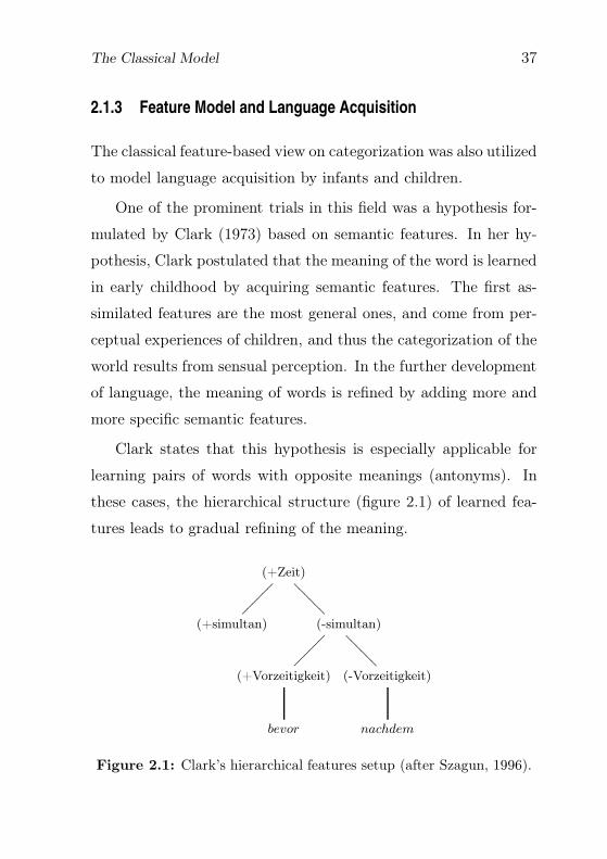
Clark states that this hypothesis is especially applicable for
learning pairs of words with opposite meanings (antonyms). In
these cases, the hierarchical structure (figure 2.1) of learned fea-
tures leads to gradual refining of the meaning.
(+Zeit)
(+simultan)
(-simultan)
????
??
(+Vorzeitigkeit)
bevor
(-Vorzeitigkeit)
????
??
nachdem
Figure 2.1: Clark’s hierarchical features setup (after Szagun, 1996).

38 MODELS OF CATEGORIZATION
The explanation of learning the meaning by acquiring seman-
tic features from perceptual experience is, however, not sufficient.
One of the unclarities was the way how sensual experiences can
change into abstract semantic features. Moreover, the theory
could not explain the meaning of words which cannot be expressed
in terms of perception (like animal or friendship) (cf. Carey, 1982;
Szagun, 1983).
Finally, other empirical studies showed that Clark’s hypoth-
esis can be applied to explain only few special cases of meaning
acquisition, namely in case of contrasting words. When the set of
words to disambiguate was broader (i.e. not limited to contrasting
words), the experiments (cf. Kavanaugh, 1976; Wannemacher and
Ryan, 1978) showed that if a child did not understand a given
word (e.g. before), it did not necessarily imply that it had the
opposite meaning (e.g. after).
2.2 Non-Classical Models
The classical view of categorization outlined so far was challenged
in the twentieth century by many philosophers and psychologists.
Some drawbacks of the classical view were spotted by Wittgen-
stein (1971). He analyzed a category of games, and came to the
conclusion that not only there are no common features to all games
but also some games are considered as better members of the
category than others.
Non-Classical Models 39
„Betrachte z.B. einmal die Vorgänge, die wir “Spiele”
nennen. Ich meine Brettspiele, Kartenspiele, Ballspiel,
Kampfspiele, usw. Was ist allen diesen gemeinsam?
– Sag nicht: “Es muß ihnen etwas gemeinsam sein,
sonst hießen sie nicht »Spiele«” – sondern schau ob
ihnen allen etwas gemeinsam ist. – Denn, wenn du
sie anschaust, wirst du zwar nicht etwas sehen, was
allen gemeinsam wäre, aber du wirst Ähnlichkeiten,
Verwandtschaften, sehen, und zwar eine ganze Reihe.
Wie gesagt: denk nicht, sondern schau! – Schau z.B.
die Brettspiele an, mit ihren mannigfachen Verwandt-
schaften. Nun geh zu den Kartenspielen über: hier
findest du viele Entsprechungen mit jener ersten Klas-
se, aber viele gemeinsame Züge verschwinden, andere
treten auf. Wenn wir nun zu den Ballspielen überge-
hen, so bleibt manches Gemeinsame erhalten, aber
vieles geht verloren. – Sind sie alle “unterhaltend”?
Vergleiche Schach mit dem Mühlfahren. Oder gibt es
überall ein Gewinnen und Verlieren, oder eine Konkur-
renz der Spielenden? Denk an die Patiencen. In den
Ballspielen gibt es Gewinnen und Verlieren; aber wenn
ein Kind den Ball an die Wand wirft und wieder auf-
fängst, so ist dieser Zug verschwunden. Schau, welche
Rolle Geschick und Glück spielen. Und wie verschie-
den ist Geschick im Schachspiel und Geschick im Ten-
40 MODELS OF CATEGORIZATION
nisspiel. Denk nun an die Reigenspiele: Hier ist das
Element der Unterhaltung, aber wie viele der anderen
Charakterzüge sind verschwunden! Und so können wir
durch die vielen, vielen anderen Gruppen von Spielen
gehen, Ähnlichkeiten auftauchen und verschwinden se-
hen.
Und das Ergebnis dieser Betrachtung lautet nun: Wir
sehen ein kompliziertes Netz von Ähnlichkeiten, die
einander übergreifen und kreuzen. Ähnlichkeiten im
Großen und Kleinen.” (Wittgenstein, 1971, p. 48)
This analysis conducted by Wittgenstein illustrated that there
exist casual categories, which cannot be described with the help
of well-defined sets of features. Everyone knows what a game is,
but it is not possible to characterize all games by means of naming
what they all have in common. There exist only similarities and
relationships among them.
Wittgenstein’s findings were further confirmed by many psy-
chological investigations, most notably those conducted by Labov
(1974), Rosch (1975a,b, 1988) or Lakoff (1973). The philosophical
investigations as well as psycholinguistic experiments had shown
that a model different from the classical one was needed.
2.2.1 Rosch’s “Standard” Prototype Model
The “standard” prototype model of categorization was formed by
Rosch and her collaborators in the 1970s. Its main feature is the

Non-Classical Models 41
redefinition of the internal structure of the category (“the horizon-
tal dimension of categories”) as well as the differentiation between
categories (“the vertical dimension”) without using the legacy of
classical categorization theory.
Two main principles underlied the formation of a prototype
model: cognitive economy and perceived world structure. They
express the fact that (natural) categories are not a result of ar-
bitrary considerations or of a historical accident but rather are
motivated physiologically.
Cognitive Economy. The cognitive economy principle says that the
categorization process should provide maximum information with
minimum cognitive effort.
“To categorize a stimulus means to consider it, for pur-
poses of that categorization, not only equivalent to
other stimuli in the same category but also different
from stimuli not in the category.” (Rosch, 1988, p. 28)
The categorization process should differentiate between objects
only if those differences are relevant for a given task.
Perceived World Structure. Simple observations and common sense
considerations lead to the conclusion that the world does not al-
low any arbitrary combinations of attributes or stimuli. Thus
Rosch states that also categories and categorization processes are
influenced by the world’s structure. Moreover, what is really im-
42 MODELS OF CATEGORIZATION
portant is perceived world structure, which can vary depending on
the observer. There does not exist an arbitrary way of perception.
What the world looks like and how it is structured are strongly
dependent on who or what the subject of observation is. The
world’s image is completely different for humans and rattlesnakes,
because both these creatures use different senses with different
sensitivity.
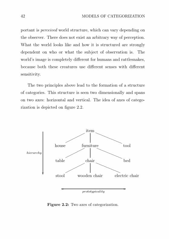
The two principles above lead to the formation of a structure
of categories. This structure is seen two dimensionally and spans
on two axes: horizontal and vertical. The idea of axes of catego-
rization is depicted on figure 2.2.
hierarchy
item
ooooooooooo
RRRRRRRRRRRRRRR
house furniture
ooooooooooo
RRRRRRRRRRRRRR tool
table chair
ooooooooooo
RRRRRRRRRRRRRR bed
stool wooden chair electric chair
ooprototypicality
//
Figure 2.2: Two axes of categorization.
Non-Classical Models 43
The Horizontal Dimension: Prototype
The horizontal dimension of categorization refers to the internal
structure of categories. In Rosch’s theory this structure is defined
in terms of prototypes.
The idea of prototypical members of categories originates from
the fact that not all members of a given category are equally good
ones. The prototypical members are those that can be said better
to represent a category better then others. In an experiment Rosch
(1975a) investigated several categories like furniture, fruit,
vehicle and others. This experiment was conducted on about
200 American students. The subjects had to answer how well ob-
jects from prepared lists represent a given category. The students
had to rate the objects in a seven-level scale. The results of this
questioning were (according to Rosch) reliable from a statistical
point of view and showed not only that graded category member-
ship is a sensible idea but also that there exist objects considered
as the best members of a given category. These ones Rosch called
prototypes.
“By prototypes of categories we have generally meant
the clearest cases of category membership defined op-
erationally by people’s judgments of goodness of mem-
bership in the category. (. . . ) [T]he more prototypical
of a category a member is rated, the more attributes
it has in common with other members of the category
44 MODELS OF CATEGORIZATION
and the fewer attributes in common with members of
the contrasting categories.” (Rosch, 1988, pp. 36–37)
Taylor (2001) mentions results obtained by René Dirven in a
similar experiment conducted on German speaking students con-
cerning the category möbel. Interestingly, this experiment shows
that although categories furniture and möbel are seen seman-
tically equivalent, their internal structure is different: the most
prototypical objects for category furniture are chair and sofa
while for category möbel there are bed and table. This inter-
language comparison shows that indeed the second principle of
categorization, the perceived world structure, has great influence
on a category’s structure formation which may vary for different
nations and languages.
Using prototypes instead of necessary and sufficient conditions
implies redefining the process of categorization. Objects have to
be categorized not by analyzing conditions or sets of features, but
by comparing them to the prototypical members. To be more
precise, the prototypes are seen as the most typical members of
a category and the other objects belong to this category if they
are similar enough to the prototypes. The prototypes thus are
cognitive reference points (Rosch, 1975a).
One has to note the difference between the terms prototype
and stereotype, which I will explain as follows. Wierzbicka (1985)
points out that:

Non-Classical Models 45
“In ordinary language, the word prototype is usually
used to refer to the original model of a certain kind
of thing (‘the first thing or being of its kind; model’,
Webster’s 1977). It is unfortunate, therefore, that in
recent literature on meaning this word has been widely
used, and in fact has become ‘institutionalized’, in a
different sense, which would have been better served
by the word stereotype.” (p. 80)
According to the tradition in linguistic literature, however, I will
use the above terms after Schwarze (1985, p. 78):
“Nous appelons prototype l’objet qui est le meilleur
exemplaire d’une catégorie, et stéréotype le concept
qui le décrit”.
In other words,
“a prototype is an object which is held to be a very
TYPICAL of the kind of object which can be referred
to by an expression containing the predicate” (Hurford
and Heasley, 2004, p. 85)
while a stereotype is
“a list of the TYPICAL characteristics of things to
which the predicate may be applied” (Hurford and
Heasley, 2004, p. 98).
Therefore, someone may have an idea of a stereotype without
being able to find an appropriate example of it (a prototype).

46 MODELS OF CATEGORIZATION
The Vertical Dimension: Basic-Level Objects
The problem of assigning an object to a given category is con-
nected to the vertical dimension of category systems. It is also
a problem of category hierarchies (taxonomies). In a taxonomy,
categories are related by means of inclusion.
Insekto
Ulod
Kapan(Grasshopper)
Lipit-lipit(Leaffolder)
Langaw-langaw(Whorlmaggot)
Bunhok(Leafhopper)
Dangaw-dangaw(Semi-looper)
Figure 2.3: Farmers’ classification of leaf feeding insects in Leyte,Philippines (adapted from http://www.knowledgebank.irri.org/IPM/soccomm/).
The ethnobiologist Brent Berlin examined the regularities in
the classification and naming of plants and animals among peoples
of traditional societies: So called folk taxonomies (see for exam-
ple figure 2.3) have hierarchical levels similar to formal biological
classifications of kingdom, phylum, class, order, family, genus and
species. Berlin (1992) states that categories are related by inclu-
siveness and also that there is a preferential level of categorization:
a basic level called folk genus. Folk genera often do not correspond
to scientific genera, but, based on cultural tradition, serve as the
most informative level in a given society.
The vertical structure of categories in Rosch’s model emerges
from the idea of folk genera. Within her model she has suggested
three levels of categorization:

Non-Classical Models 47
• superordinate,
• basic level, and
• subordinate.
The key word for learning hierarchy of categories in Rosch’s
model is the basic-level category. The experiment in which sub-
jects had to list as many attributes as possible for objects in classes
designated by names of categories from different levels was con-
ducted. Similar experiments involved also listing of motor move-
ments and comparison of simplified shapes of objects.
“For all the taxonomies studied, regardless of whether
language dependent variables such as attributes or lan-
guage independent variables such as shape were used,
there was a level of abstraction at which all factors co-
occurred and below which further subdivisions added
little information.” (Rosch et al., 1976, p. 428)
Basic-level categories can thus be described as information-
rich bundles of co-occurring perceptual and functional attributes.
According to Kleiber (2003) their psycholinguistic importance ma-
nifests itself in many ways outlined below.
The basic-level is the highest level of abstraction where it is
possible to construct a Gestalt of an object (Berlin, 1992). There
is a general form of a chair, but no general form for furniture.
This is directly connected to the fact that on the basic-level it is
possible to create an image (abstract or concrete) representing the
48 MODELS OF CATEGORIZATION
whole category. Trying to create an image of an object from super-
ordinate category one either ends up with an object which in fact
belongs to a basic-level category or one is not able to accomplish
this task at all.
Motoric movements (for categories to which they apply) are
similar for all objects contained in basic-level (Rosch, 1988). And
again, in the example mentioned above, it is possible to imagine
or describe the process of using a chair while there is no general
routine for using furniture.
From the purely psychological point of view, basic-level cate-
gories also manifest their existence in several ways (Rosch et al.,
1976): In the task of categorization, assigning objects to basic-
level category is faster than to other levels of abstraction. It
results, among other things, in more frequent use of names of
those objects in naming tasks. Directly connected with this phe-
nomenon is the fact that basic-level categories are the first and
fundamental categories learned by children.
The basic-level of categorization manifests itself also in lan-
guage usage. Terms denoting objects on the basic-level are context
neutral (cf. Cruse, 1977; Lakoff, 1987). They also usually define
the choice of pronouns. Usage of super- or subordinate term is
most often motivated by a context, while in context-neutral ut-
terances people tend to choose basic-level terms.
Non-Classical Models 49
The Importance of the Prototype Model
The most important consequence of the development of the proto-
type model was the creation of an alternative to the Aristotelian-
like way of categorizing. It is of great importance to have other
categorization models because, as mentioned above, the classical
model does not explain psychological data gathered. Indeed, the
prototype model has a much greater explanation power. Accord-
ing to Lakoff (1987), not only categories of concepts have proto-
typical properties but also linguistic categories can be described
in this way. This author suggests that language categories have
the same structure as categories of concepts.
The prototypical view on category structure solves also many
problems with the internal structure of categories. It explains
blurred borders of categories as well as the intuitive property that
not all members represent the category equally well. The proto-
type model allows for the categorization of marginal cases, which
is hard to describe within classical theory. For example, it makes
no problem to categorize a one-legged chair as a chair, while it
would be extremely hard if not impossible to conceive a set of
rules describing all possible chairs.
In semantics, the prototype theory allows for describing mean-
ings in terms of “information density” (Geeraerts, 1986). This
gives much more flexibility in defining sets of properties needed
for such a description: the prototypical conception organizes cat-
egories such that they are clusters of concepts and nuances. Ac-
50 MODELS OF CATEGORIZATION
cording to Wierzbicka (1985), one should, however, differentiate
between significant properties and prototypical properties. The
significant ones refer to “semantic primitives” and are those which
guarantee that an object which possesses them is indeed a mem-
ber of the category in question. The latter ones are typical for a
category but not obligatory.
Problems of the Prototype Model
Unfortunately, the prototype model outlined so far is not the magi-
cal answer to all problems concerning categorization processes and
category structure. It also suffers from several shortcomings.
Although the prototype model was created as a counterpro-
posal for categorization based on necessary and jointly sufficient
conditions it cannot completely get rid of this formalism. The
vertical axis of categorization is based on class inclusion which in
turn is based on the implication relation. The implication relation
however needs the reference to necessary conditions. It means that
although the return to necessary and jointly sufficient conditions
is not compulsory, there must be at least a trail of necessary con-
ditions: a set of features may not be equivalent to a characteristic
of category but it implies that an object being a member of the
category de facto has those features.
Osherson and Smith (1981) investigated the prototype cate-
gory in terms of two criteria: the relationship between complex
concepts and their conceptual constituents and the truth condi-
Non-Classical Models 51
tions of thoughts corresponding to the simple inclusions. The au-
thors evaluated those issues by means of Zadeh’s theory of fuzzy-
sets (Zadeh, 1965, 1975) which was also used by Rosch (1975b)
to represent the prototype model formally. The final conclusion
of their work was threefold: either a prototype theory cannot be
represented with the fuzzy-set formalism, or the prototype theory
should be negated completely – what is however not recommended
because this theory captures many ideas about categorization –
or prototype theory is not complete and applies only to limited
aspects of concepts.
“[W]e can distinguish between a concept’s core and its
identification procedure; the core concerns with those
aspects of concept that explicate its relation to other
concepts, and to thoughts, while the identification pro-
cedure specifies the kind of information used to make
rapid decisions about membership. (. . . ) Given this
distinction it is possible that some traditional theory
of concepts correctly characterizes the core, whereas
prototype theory characterizes an important identifi-
cation procedure.” (Osherson and Smith, 1981, p. 57)
The above shows that not all kinds of categories are equally
well described by prototype theory. The best ones are naturally
those which served as a base for this theory: perceptual categories,
natural categories, artifacts etc. The most problems are connected
with compositional concepts.

52 MODELS OF CATEGORIZATION
The problems with “standard” prototype theory can be solved
in two ways. Either by application of prototype theory to the
prototype itself or by redefining the mechanisms underlying the
categorization.
The notion of prototypicality as characterized by Geeraerts is
founded by four properties:
1. Prototypical categories cannot be defined by means
of a single set of criterial (necessary and suffi-
cient) attributes. (. . . )
2. Prototypical categories exhibit a family resem-
blance structure, or more generally, their seman-
tic structure takes the form of a radial set of clus-
tered and overlapping meanings. (. . . )
3. Prototypical categories exhibit degrees of cate-
gory membership; not every member is equally
representative for a category. (. . . )
4. Prototypical categories are blurred at the edges.(. . . )
(Geeraerts, 1988, pp. 343–344)
Following this author one can notice that not all of the above
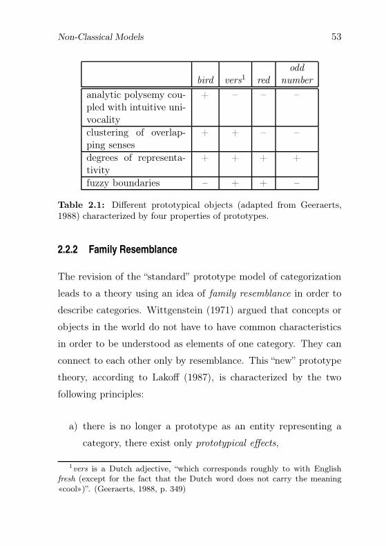
properties apply to all cases of prototypical objects (cf. table 2.1).
Different prototypes can represent different properties of prototyp-
icality and this means that a prototype is indeed autoprototypical.
In fact, this characteristic of prototype leads to the next version
of theory of prototype, the theory of family resemblances.
Non-Classical Models 53
oddbird vers1 red number
analytic polysemy cou-pled with intuitive uni-vocality
+ – – –
clustering of overlap-ping senses
+ + – –
degrees of representa-tivity
+ + + +
fuzzy boundaries – + + –
Table 2.1: Different prototypical objects (adapted from Geeraerts,1988) characterized by four properties of prototypes.
2.2.2 Family Resemblance
The revision of the “standard” prototype model of categorization
leads to a theory using an idea of family resemblance in order to
describe categories. Wittgenstein (1971) argued that concepts or
objects in the world do not have to have common characteristics
in order to be understood as elements of one category. They can
connect to each other only by resemblance. This “new” prototype
theory, according to Lakoff (1987), is characterized by the two
following principles:
a) there is no longer a prototype as an entity representing a
category, there exist only prototypical effects,
1vers is a Dutch adjective, “which corresponds roughly to with Englishfresh (except for the fact that the Dutch word does not carry the meaning«cool»)”. (Geeraerts, 1988, p. 349)

54 MODELS OF CATEGORIZATION
b) the relation between members of the same category is a fam-
ily resemblance relation.
This idea is in some sense reversed in comparison to the former
prototype model. The prototypical effects in a category are now
only a consequence of the relationship between its members.
This change in the categorization principle leads at first to the
change in category structure from radial one (cf. figure 2.4 for
a category bird) to the more distributed structure where indeed
a prototypical kernel exists, but where also outlying exemplars
occur which not necessarily have any properties common with
those forming the prototype (figure 2.5).
Figure 2.4: The radial structure of category.
This new category structure is based on family resemblance
(Wittgenstein, 1971). In the “standard” version of prototype the-
ory the notion of family resemblance was also introduced but (as
suggested by Kleiber, 2003) it was used improperly and motivated
by its false identification with similarity to the prototype.
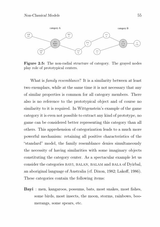
Non-Classical Models 55
A CB D FE G
B FC
C FG
A BI C
E DK
F Gz
z xy
y uv
z xy uv w
uv w
category A category B
Figure 2.5: The non-radial structure of category. The grayed nodesplay role of prototypical centers.
What is family resemblance? It is a similarity between at least
two exemplars, while at the same time it is not necessary that any
of similar properties is common for all category members. There
also is no reference to the prototypical object and of course no
similarity to it is required. In Wittgenstein’s example of the game
category it is even not possible to extract any kind of prototype, no
game can be considered better representing this category than all
others. This apprehension of categorization leads to a much more
powerful mechanism: retaining all positive characteristics of the
“standard” model, the family resemblance denies simultaneously
the necessity of having similarities with some imaginary objects
constituting the category center. As a spectacular example let us
consider the categories bayi, balan, balam and bala of Dyirbal,
an aboriginal language of Australia (cf. Dixon, 1982; Lakoff, 1986).
These categories contain the following items:
Bayi : men, kangaroos, possums, bats, most snakes, most fishes,
some birds, most insects, the moon, storms, rainbows, boo-
merangs, some spears, etc.

56 MODELS OF CATEGORIZATION
Balan : women, anything connected with water or fire, bandi-
coots, dogs, platypus, echidnae, some snakes, some fishes,
most birds, fireflies, scorpions, crickets, the stars, shields,
some spears, some trees, etc.
Balam : all edible fruit and the plants that bear them, tubers,
ferns, honey, cigarettes, wine, cake.
Bala : parts of the body, meat, bees, wind, yam sticks, some
spears, most trees, grass, mud, stones, noises, language, etc.
Clearly there is no single object which could serve as a center for
each of these categories. However all of the elements are connected
to each other by having at least one overlapping property. For
example the moon in bayi category is related to men, because in
myths it is personified as a husband. Analogously, the sun is in
the same category as women, because in myths it is incarnated as
a wife.
Actually, the term prototype should be replaced with the term
prototypical effect. Fillmore (1982), Lakoff (1987) and Geeraerts
(1988) suggest many types of prototypical effects dependent on the
type of category in question. That is why a prototype becomes
only a surface effect and cannot be used directly to build up a
category structure.
Non-Classical Models 57
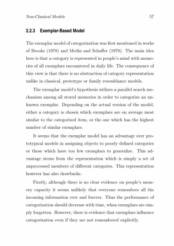
2.2.3 Exemplar-Based Model
The exemplar model of categorization was first mentioned in works
of Brooks (1978) and Medin and Schaffer (1978). The main idea
here is that a category is represented in people’s mind with memo-
ries of all exemplars encountered in daily life. The consequence of
this view is that there is no abstraction of category representation
unlike in classical, prototype or family resemblance models.
The exemplar model’s hypothesis utilizes a parallel search me-
chanism among all stored memories in order to categorize an un-
known exemplar. Depending on the actual version of the model,
either a category is chosen which exemplars are on average most
similar to the categorized item, or the one which has the highest
number of similar exemplars.
It seems that the exemplar model has an advantage over pro-
totypical models in assigning objects to poorly defined categories
or those which have too few exemplars to generalize. This ad-
vantage stems from the representation which is simply a set of
unprocessed members of different categories. This representation
however has also drawbacks.
Firstly, although there is no clear evidence on people’s mem-
ory capacity it seems unlikely that everyone remembers all the
incoming information ever and forever. Thus the performance of
categorization should decrease with time, when exemplars are sim-
ply forgotten. However, there is evidence that exemplars influence
categorization even if they are not remembered explicitly.

58 MODELS OF CATEGORIZATION
Barsalou (1992, pp. 27–28) mentions even more serious flaws
in the exemplar-based model. People are clearly able to abstract
from exemplars and to create general representations for cate-
gories. The exemplar model – by definition – can explain neither
forming of those abstractions nor their use.
2.3 No Clear-Cut Between Models
Experimental data known so far shows clearly that the classi-
cal feature-based model of categorization is not sufficient. But it
cannot be completely rejected. Even in the most sophisticated
prototype-based models the comparison process is built in.
The prototype models of categorization “simply” compare an
object to be categorized with some set of prototypes or other mem-
bers of a category. The problem is how this comparison is being
done. Rosch’s experiment (1976) concerning objects’ shapes may
suggest that the comparison is a kind of pattern matching: an
object is said to be a member of a given category when it is most
similar to the pattern of a prototype for this category. But as
Harnad (2003) points out
“it is simply not the case that everything is a member
of every category, to different degrees. It is not true
ontologically that a bird is a fish (or a table) to a
certain degree; nor is it true functionally that sensory
shadows of birds can be sorted on the basis of their
degree of similarity to prototype birds, fish or tables.”
Learning Categories 59
The same problem occurs with the family resemblance mecha-
nism. It says that members of categories are similar to each other
to some degree. Again, the question is how to measure this sim-
ilarity if not on the feature basis? Similarly, the exemplar-based
model suffers from this dilemma.
Kleiber (2003) points out that the prototype model actually
describes categories also in terms of features (or properties). The
feature mechanism is thus inherent within these more “psychologi-
cally justified” models. Thus a prototype can be defined as the set
of the most common features within a category and similarity can
be measured by the number of features and the degree to which
they match the prototype. Similarly family resemblance could be
defined by measuring the number of common properties and the
degree to which they overlap.
2.4 Learning Categories
The prototype, family resemblance and exemplar-based theories
describe phenomena related to categorization and category struc-
ture. However, none of those mechanisms explains how the cate-
gory structure is obtained. Indeed comparing either to prototype,
to other category members or using the set of rules requires that
the category structure is already present. Thus, no matter what
mechanism we assume to be appropriate for describing a category
structure, a learning method has to be also defined.
60 MODELS OF CATEGORIZATION
Ashby and Maddox (2005) enumerates four main methods
most commonly used for investigating category learning by hu-
mans.
Rule-based. Rule-based category learning is generally a method
by which a subject learns the rules. These rules describe
the strategy of categorization verbally. Several conditions
must be met in this case: each stimulus must have a seman-
tic label, the subject must be able to isolate each property
of stimulus, and the rule combining information from differ-
ent stimuli must be verbalizable (usually in terms of logical
operations).
Information integration. In this learning method categoriza-
tion is possible only if information from several sources is
integrated on the pre-decision stage.
Prototype distortion. Learning randomly distorted single cat-
egory prototype is a base for the prototype distortion metod.
There are two popular variations: (A, B) and (A, not A). In
the former, exemplars from category A are presented against
exemplars from the contrasting category B. In the latter
method there is only one category presented in contrast to
exemplars not attributed to any category.
Weather prediction. This last method has the goal of finding
out whether a membership in category is deterministic or
probabilistic. In deterministic learning each stimulus has un-

Learning Categories 61
ambiguously assigned a member of a given category, whereas
in probabilistic tasks at least some of the stimuli are ran-
domly associated to more different categories.
Although it is not clear which of the above methods describes
category learning by humans (if any) there are different phenom-
ena connected with category acquisition. One of them is asymmet-
ric category learning (cf. Quinn et al., 1993) which is investigated
in the following chapters.
In the current chapter the models of categorization provided by
literature have been outlined. These models constitute a basis
for judging the categorization model I propose in this paper. This
model is a connectionist one. Thus, the following chapter presents
those aspects of connectionism which are needed to define the
model.

CHAPTER 3
Connectionism
Connectionism is nowadays one of the theories of information pro-
cessing within cognitive sciences (Medler, 1998). The term “con-
nectionism” itself originates from the idea of representing a system
as a net built of nodes and connections, where the main informa-
tion is stored in connections. The categorization model described
in this work deals with creating a taxonomy of concepts, formed as
a network of interconnected nodes. Thus, from the architectural
point of view, the model presented can and should be regarded as
a variant of a connectionist system. Moreover, the data process-
ing within this model involves passing a signal from one node to
the others which is a common procedure in connectionist models
63
64 CONNECTIONISM
known as activation spreading. The task of this chapter is to show
what connectionism is and how it is related to the categorization
model.
Connectionism is regarded as the main alternative to a sym-
bolic processing in cognitive sciences, especially in psycholinguis-
tics. Figure 3.1 presents the hierarchy of main types of cognitive
models currently developed. According to this classification, con-
nectionist models belong to the class of quantitative, algorithmic
ones. Further, they subdivide into two branches: localist mod-
els and parallel distributed processing ones. Actually, the localist
models are also based on parallel distributed processing, but the
difference (as will be explained later) is in the data representation
used.
The current chapter is divided as follows. The Section 3.1
presents briefly the history of connectionist modeling. The follow-
ing Section 3.2 explains the place of connectionist models within
the model theory. Section 3.3 deals with data representation used
in different flavors of connectionist models. The next two Sec-
tions, 3.4 and 3.5, describe in more detail distributed and localist
types of connectionism respectively. Semantic networks, which
are structures slightly similar to the connectionist networks, are
highlighted in Section 3.6. Then, the opposition between brain
structure and connectionist models is described in Section 3.7.
Possible approaches to language processing in the connectionist
context are discussed briefly in Section 3.8. Finally Section 3.9

On the History of Connectionism 65
explains how the model of categorization presented in this work
can be defined as a connectionist model.
Cognitive Models
prequantitative
V-type
quantitative??
????
M-type
A-type??
????
symbolic
connectionist
????
???
localist
PDP??
????
?
Figure 3.1: Hierarchy of different cognitive models (after Grainger andJacobs, 1998). The leaf and branch names have the following meanings.V-type: verbal and boxological, M-type: mathematical, A-type: algo-rithmic, computational.
3.1 On the History of Connectionism
Network models come to light in 1940’s when McCulloch and Pitts
(1943) proved that networks of simple interconnected binary units,
when supplemented by indefinitely large memory, were compu-
tationally equivalent to a Turing’s universal computing machine
(Turing, 1937). For these kinds of machines, Turing proves:
“It is possible to invent a single machine which can be
used to compute any computable sequence.” (Turing,
66 CONNECTIONISM
1937, p. 241)
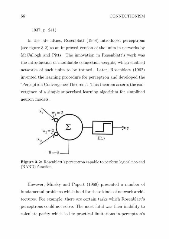
In the late fifties, Rosenblatt (1958) introduced perceptrons
(see figure 3.2) as an improved version of the units in networks by
McCullogh and Pitts. The innovation in Rosenblatt’s work was
the introduction of modifiable connection weights, which enabled
networks of such units to be trained. Later, Rosenblatt (1962)
invented the learning procedure for perceptron and developed the
“Perceptron Convergence Theorem”. This theorem asserts the con-
vergence of a simple supervised learning algorithm for simplified
neuron models.
Figure 3.2: Rosenblatt’s perceptron capable to perform logical not-and(NAND) function.
However, Minsky and Papert (1969) presented a number of
fundamental problems which hold for these kinds of network archi-
tectures. For example, there are certain tasks which Rosenblatt’s
perceptrons could not solve. The most fatal was their inability to
calculate parity which led to practical limitations in perceptron’s
On the History of Connectionism 67
application. For example, a perceptron could not learn to evalu-
ate the logical function of exclusive-or (XOR) and other linearly
inseparable problems. Minsky and Papert suggested the possibil-
ity of developing perceptrons into more sophisticated architecture
consisting of more processing layers. They predicted, however,
that this architecture would suffer from similar inabilities as the
single perceptron.
Another reason for suppressing the connectionist ideas of com-
putation was the success of other approaches to so-called “artificial
intelligence”. Among them were systems like STUDENT (Bobrow,
1969), Analogy Program (Evans, 1969), and a semantic memory
program called the Teachable Language Comprehender (Quillian,
1969), which seemed not to suffer from limitations of connectionist
systems.
In the seventies, not many significant studies on connectio-
nism were done. Some important exceptions were the works of
Anderson (1972), Kohonen (1972), and Grossberg (1976). Min-
sky and Papert’s prediction about the limitations of multi-layered
architectures based on a perceptron idea, however, were not con-
firmed.
In the eighties the renaissance of network architectures began.
The connectionism then split formally into localist connectionism
(McClelland and Rumelhart, 1981; Dell, 1986; McClelland and El-
man, 1986) and parallel distributed processing (Rumelhart et al.,
1986b). The network modeling gained more and more attention

68 CONNECTIONISM
also because of dissatisfaction with the results obtained with the
artificial intelligence models (cf. Graubard, 1988).
The “modern connectionism” which started in 1980s brought
computationally powerful and trainable networks — new tools for
investigating human cognition. The development of training pro-
cedures for multi-layer networks gave not only a tool computation-
ally powerful enough to model problems of cognition but also a
learning procedure to deal with those problems. Nowadays, con-
nectionism is still evolving. The different network architectures
and learning rules developed so far allow one to choose an appro-
priate tool for a specific problem.
3.2 Algorithmic Model Theory
Model theory in general is a branch of logic. In a broader sense,
model theory is the study of the interpretation of any language,
formal or natural, by means of set-theoretic structures, with Alfred
Tarski’s truth definition (Tarski, 1933) as a paradigm. In this
broader sense, model theory meets philosophy at several points,
for example in the semantics of natural languages.
Algorithmic model theory (the theory of A − type models, cf.
figure 3.1) investigates the application of model theoretic methods
to different problem domains in computational science (cf. Otto,
2002). The most interesting domain from this work’s point of
view is the domain of knowledge representation and artificial in-
telligence. Because descriptive logics are also being used as formal

Remarks on Data Representation 69
languages for knowledge representation, it is relatively straightfor-
ward to connect it with model theory.
Connectionist models form a sub-branch of the more general
class of algorithmic models. The power of A− type models is that
they can be applied as tools to analyze the functioning of cognitive
systems and processes. They, however, do not claim to provide
the true solutions. Instead they can provide an explanation of
how the system could work but not necessarily how it does work.
The A − type models, and thus the connectionist models, have
the potential to bring insights into the functionality of cognitive
systems.
In the following an overview of the two main branches of con-
nectionism, distributed connectionism and localist connectionism,
is given.
3.3 Remarks on Data Representation
To start talking formally about the connectionism, one needs at
first to consider data to be processed by the system. The form
of data being processed by the connectionist system is the central
factor that decides what properties a system should have in order
to properly model a given phenomenon. The two main types of
data representation are local and distributed (figure 3.3).
Between these two poles there exists a number of mixed rep-
resentations. In the following localist and distributed representa-
tions are shortly characterized. The description assumes that the
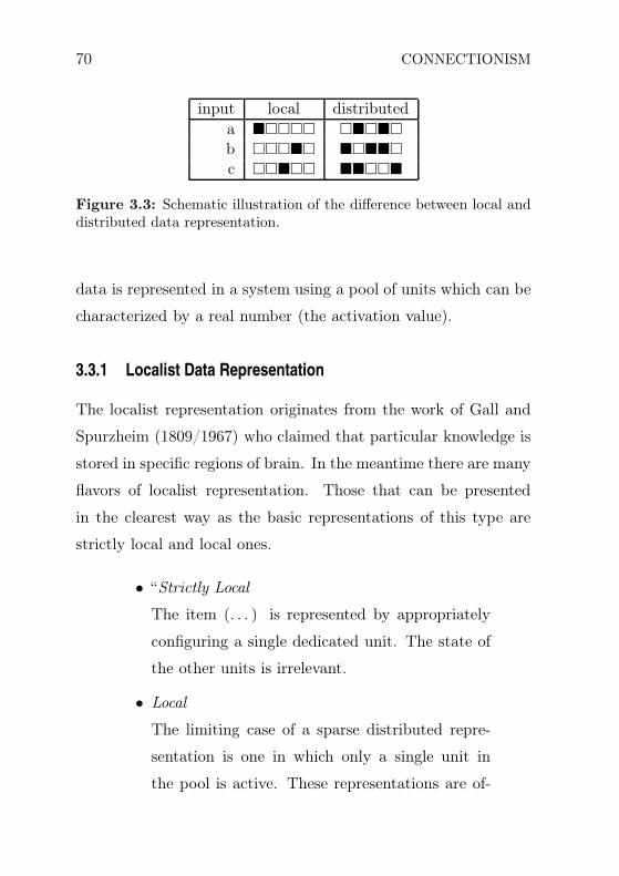
70 CONNECTIONISM
input local distributeda
b
c
Figure 3.3: Schematic illustration of the difference between local anddistributed data representation.
data is represented in a system using a pool of units which can be
characterized by a real number (the activation value).
3.3.1 Localist Data Representation
The localist representation originates from the work of Gall and
Spurzheim (1809/1967) who claimed that particular knowledge is
stored in specific regions of brain. In the meantime there are many
flavors of localist representation. Those that can be presented
in the clearest way as the basic representations of this type are
strictly local and local ones.
• “Strictly Local
The item (. . . ) is represented by appropriately
configuring a single dedicated unit. The state of
the other units is irrelevant.
• Local
The limiting case of a sparse distributed repre-
sentation is one in which only a single unit in
the pool is active. These representations are of-
Remarks on Data Representation 71
ten also referred to as “local” (. . . ). The key dif-
ference with strictly local representations is that
here it matters what state the other units in the
pool are in, viz., they must not be active.”
(van Gelder, 1999, p. 188)
3.3.2 Distributed Data Representation
On the other end of the representation spectrum there is dis-
tributed representation. This representation assumes that spe-
cific information is represented by more than just one unit. In
addition, each single unit contributes to many representations. In
other words, it is usually the case that the same subset of units
can code many different pieces of information by means of differ-
ent activation patterns. It means that no single unit holds enough
clues to decode the information stored in the system’s pool of data
representing items.
3.3.3 Meaning of a Unit
Another aspect of local versus distributed data representation op-
position refers to the meaning and the interpretation of a single
item used to store data. The simplest way to deal with it is to
say that in localist systems each unit carries its own independent
piece of information which can be interpreted without taking the
state of other system’s parts into account. Even if the overall in-

72 CONNECTIONISM
formation is composed of multiple units, each one is independent.1
Thorpe (1995) formulates this characteristic in the following way:
“With a local representation, activity in individual
units can be interpreted directly. [W]ith distributed
coding individual units cannot be interpreted without
knowing the state of other units in the network.”
On the other hand, the distributed data representation makes
clear that the meaning of a single, separated unit is useless. Only
the overall state of the whole system carries meaningful informa-
tion. This representation has its advantages (for example in case
the system is partially damaged, because even then the data may
be restored with some accuracy) but also disadvantages (e.g. very
complicated ways to analyze the correlations between different
pieces of data).
3.3.4 Semantic Problems
Talking about local and distributed representation always involves
formal, semantic problems. The terms “local” and “distributed” are
usually used in literature in many different ways and are in fact
still not well defined as yet.
Page (2000) argues that the real localist systems can use only
the strictly local representation. Moreover, what counts is not
1This kind of representation where the meaning in macro-scale is composedof the state of many strictly local units is often referred to as representationby microfeatures.

Distributed Connectionism 73
the input and output signal form but the way it is processed.
However many connectionist systems (eg. Dell, 1986; McClelland
and Elman, 1986; Schade, 1999) are usually seen as localist ones,
although they use not strictly local data representation for pro-
cessing. This view can be justified by grouping representation
units into layers and considering each layer as a different subsys-
tem with its own, independent data representation. However, it
still leaves the problem of localist and distributed representations
vague.
In the following the short characteristics of sample systems
using distributed or localist representation are given.
3.4 Distributed Connectionism
A distributed connectionist, sometimes referred to as artificial
neural networks, is a computational method derived from obser-
vations about brain structure and properties of neurons. Such a
network consists of a (usually) large number of simple processing
units, called (artificial) neurons or just nodes. These nodes are
interconnected by weighted links.
The main principles of connectionist models derived from gen-
eral observations about the brain are as follows (according to
McLeod et al., 1998):
1. An artificial neuron receives and sums up input signals.
Based on this sum the neuron’s actual activation value is
74 CONNECTIONISM
calculated and passed during the next step as an actualized
signal via weighted connections to other nodes.
2. The artificial neural networks are usually organized in lay-
ers and connections exist mainly between nodes in adjacent
layers. There are in general no connections between nodes
in the same layer or the connections have a different nature
than inter-layer ones.
3. The influence of one neuron on another one depends on
the strength of the connection between them (connection
weight).
4. The weights’ values are obtained during a learning process.
Due to the nature of input and output data (real-valued vec-
tors) neural networks are often used to approximate real-valued
functions. Because of this feature, neural networks may be called
universal approximators, and they are exploited to estimate un-
known (or very complicated) relationships.
3.4.1 The Artificial “Neuron”
An artificial neuron, often called a node, is a simple processing
unit which is a further development of Rosenblatt’s perceptron (cf.
page 66). Its role is to calculate an activation value (according
to some given function) out of the input data. The input data
consists of signals from many other nodes, and the activation value

Distributed Connectionism 75
is used as the node’s output signal during the next step. The
schema of an artificial neuron is drawn in figure 3.4.
Figure 3.4: An artificial neuron.
In order to calculate the activation value, an activation func-
tion is used. Its concrete form is task-dependent. The standard
and probably most often used activation function is derived from
a logistic function (Kingsland, 1995):
P (t) = a1 + me−t/τ
1 + ne−t/τ(3.1)
The special case of logistic function (3.1) used in parallel dis-
tributed modeling is called a “sigmoidal function” (equation 3.2)
due to the sigmoid shape of its graph (see figure 3.5) or a “stan-

76 CONNECTIONISM
dard logistic function” (cf. for example McLeod et al., 1998; Ellis
and Humphreys, 1999)
f(si) =1
1 + e−si
(3.2)
0
0.2
0.4
0.6
0.8
1
-6 -4 -2 0 2 4 6
Figure 3.5: Sigmoidal (standard logistic) function.
In (3.2), si is the sum of the weighted outputs of those nodes
which are connected to the node i, as given in equation 3.3
si =∑
j
wjiaj (3.3)
In (3.3), wji denotes the weight of the connection from node j to
node i and aj is the activation value of node j.

Distributed Connectionism 77
3.4.2 Basic Architecture
There exists a large number of possible network architectures (i.e.
ways how nodes are organized and connected). The most popular
are so-called feed-forward networks in which a signal is propagated
only in one direction: from the layer of input neurons through one
or more hidden layers to the layer of output neurons. The name
“hidden layer” means that that activation value patterns in those
layers are not visible to the user.
In the following subsection the most basic network architec-
ture is described as it is a starting point for many investigations
involving distributed connectionist models.
Multi-Layer Perceptron (MLP)
A multi-layer perceptron is the most common neural network ar-
chitecture. Two-layer perceptrons were first introduced by Rosen-
blatt (1958). The multi-layer version of perceptron has been pro-
posed by Rumelhart et al. (1986b). Picture 3.6 shows the schema
of the latter. The nodes are organized in three layers. One layer
is the input layer (i.e. the activation of nodes in this layer, input
nodes, depends directly on input data) and one layer is the output
layer (i.e. this layer’s nodes’ activation pattern is considered to
be the output of the network). The intermediate layer is called
hidden because its activation distribution is not directly accessible
for a user.

78 CONNECTIONISM
output layer ?>=<89:; ?>=<89:; · · · ?>=<89:;
input layer ?>=<89:; ?>=<89:; ?>=<89:; ?>=<89:; · · · ?>=<89:;
hidden layer ?>=<89:;
nnnnnnnnnnnnnnnnnnnnnnnnn
))))
))))
)
<<<<
<<<<
<<<<
<
JJJJJJJJJJJJJJJJJJ
SSSSSSSSSSSSSSSSSSSSSSSSSSSSSSSS ?>=<89:;
)))))))))
tttttttttttttttttt
))))
))))
)
<<<<
<<<<
<<<<
<
PPPPPPPPPPPPPPPPPPPPPPPPP ?>=<89:;
<<<<<<<<<<<<<
)))))))))
tttttttttttttttttt
))))
))))
)
JJJJJJJJJJJJJJJJJJ · · · ?>=<89:;
PPPPPPPPPPPPPPPPPPPPPPPPP
JJJJJJJJJJJJJJJJJJ
)))))))))
kkkkkkkkkkkkkkkkkkkkkkkkkkkkkkkk
nnnnnnnnnnnnnnnnnnnnnnnnn
tttttttttttttttttt
))))
))))
)
Figure 3.6: Multi-layer perceptron schema. Circles stand for nodesand lines for connections between them.
The multi-layer perceptron is a kind of feed–forward network,
which means signals flow in only one direction: from input layer
through hidden layers to output layer without any back loops.
3.4.3 Learning
In the case of artificial neural networks, learning is a process of
changing connection weights. Usually feed-forward distributed
networks are trained according to a supervised method of learn-
ing (cf. le Cun, 1985; Parker, 1985; Rumelhart et al., 1986a). The
main attribute of supervised learning is that it needs a large num-
ber of input and output data pairs.
There exists a number of different supervised learning meth-
ods, rules and algorithms. For a multi-layer perceptron the most

Distributed Connectionism 79
common method is called error back-propagation (cf. Rumelhart
et al., 1986a). The principle of this algorithm is the following.
1. The network is presented with input data selected (usually
randomly) from the set of training data.
2. The output is calculated according to the activation func-
tion.
3. The output is compared with the desired result and out of
this comparison the output layer error is calculated.
4. Based on the error found in step 3 and the current con-
nection weights errors are calculated for the other network
layers as well (“backpropagated”).
5. Based on the errors calculated in steps 3 and 4 and the
existing connection weights, all the weights are modified.
The weights’ changes are usually controlled by two parameters:
• learning rate, which is simply a fraction of an error value
taken into account when changing weights,
• learning momentum, which is a fraction of previous weight
changes. The learning momentum is used to prevent the
learning procedure being captured in a local minimum of
the learned function.
Usually learning is applied until a given performance of the net-
work is reached, that is, until the error rate decreases below some

80 CONNECTIONISM
acceptable level. In most applications, learning is done only once.
After that the artificial neural network is used. After learning all
weights remain fixed.
Until the back-propagation algorithm was presented, it was
not possible to train perceptrons of more than two-layer. This
algorithm definitely overcame the limitations of the first connec-
tionist architectures which had been noted by Minsky and Papert
(1969), and allowed for serious competition against the symbolic
approach.
As the “extension” of multi-layer perceptron architecture there
were two other network types proposed by Jordan (1986) and
Elman (1990) in order to learn and process time sequences of
input activation patterns. These networks contain one additional
layer of units, called the “context layer”. The task of the context
layer is to provide a short-term memory for a network. The differ-
ence between Jordan and Elman network types is that the former
expresses context in terms of activation pattern of output nodes
in the previous time-step of processing and the latter in terms of
activation pattern of a hidden layer. The presence of short-term
memory allows for processing sequences of input patterns, or, more
precisely, for processing an input signal in context of previously
processed ones. These architectures were the first ones which gave
the possibility to train networks on sequences of arbitrary length,
thus allowing for real language processing (for example, extracting
grammar rules from sample sentences, cf. Lawrence et al., 2000).

Distributed Connectionism 81
The multi-layer perceptron and architectures derived from it
have become a flagship for “modern connectionism” in its dis-
tributed version. They were successfully used also for categoriza-
tion purposes (e.g. McClelland and Rumelhart, 1985; Kruschke,
1992; Dienes, 1992). The fatal disadvantage of distributed connec-
tionist categorization models is that it is not possible in a simple
way (cf. cluster analysis, Tryon, 1939) to retrieve the dependen-
cies among learned categories, that is, the taxonomical structure.
That is why, in my opinion, distributed connectionism alone is not
the optimal solution for a categorization model.
3.4.4 Self-Organizing Maps
Another interesting artificial neural network architecture is a self-
organizing map (SOM), originally proposed by Kohonen (1982).
Those networks use so-called unsupervised learning (Hinton and
Sejnowski, 1999) in which a model fits to observed data. In un-
supervised learning, in contrast to supervised learning used in
multi-layer perceptrons, the desired output is not defined.
The objective of SOM is to map the input data onto a multi-
dimensional array. The most popular are, however, two- and
three-dimensional maps. Each node in the network is charac-
terized by an n-dimensional vector containing some data Wij =
(w1, . . . , wn) and its physical location in the network. Like most
connectionist systems, SOMs also operate in two modes:

82 CONNECTIONISM
1. Training (learning) mode.
In the training mode, the network organizes itself using com-
petitive algorithms (e.g. winner-take-all). The organization
is executed in the following way: the input data in form of
a vector is presented, the node with the data vector which
is most similar to the input one is chosen, and the vector
is modified in a way to make it more similar to the input
data. This process is repeated for all input data and usually
in many cycles.
2. Production (mapping) mode.
In mapping mode, the input vector is compared to the vec-
tors of all network nodes and the most similar one is chosen.
The “winning” node can be physically localised and classified
based on the location on the map.
Kohonen networks are often used for classification (or cate-
gorization) (Anderson and Mozer, 1989; Merkl, 1998), data com-
pression (Amerijckx et al., 2003; Seiffert, 2005), pattern recogni-
tion (Carpenter and Grossberg, 1991; Ghosh and Pal, 1992) or to
visualize large collections of data (e.g. WebSOM by Lagus et al.,
1999, see figure 3.7).
The interesting (from the categorization point of view) prop-
erty of self organizing maps is that they preserve the topology of
input data. This means that similar input data are associated
with the nodes in the network which have similar physical posi-
tions (cf. figure 3.7). This property makes SOM into a tool for

Distributed Connectionism 83
Figure 3.7: WebSOM example: the map of articles from usenet groupcomp.ai.neural-nets. The labels denote sample posts from thegroup. Similar articles are placed near each other on the map (topologypreserving property). The color represents the density of documents:light areas contain more documents. (From: http://websom.hut.fi/websom/.)
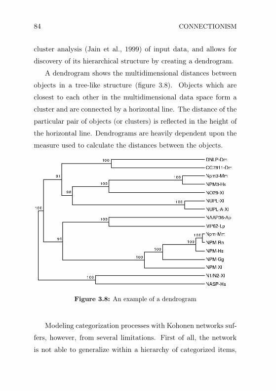
84 CONNECTIONISM
cluster analysis (Jain et al., 1999) of input data, and allows for
discovery of its hierarchical structure by creating a dendrogram.
A dendrogram shows the multidimensional distances between
objects in a tree-like structure (figure 3.8). Objects which are
closest to each other in the multidimensional data space form a
cluster and are connected by a horizontal line. The distance of the
particular pair of objects (or clusters) is reflected in the height of
the horizontal line. Dendrograms are heavily dependent upon the
measure used to calculate the distances between the objects.
Figure 3.8: An example of a dendrogram
Modeling categorization processes with Kohonen networks suf-
fers, however, from several limitations. First of all, the network
is not able to generalize within a hierarchy of categorized items,

Localist Connectionism 85
in the sense that unknown objects do not correspond to any node
in the dendrogram. The only “generalization” possible is to judge
which known object the input data is most similar to. Secondly,
the limited number of nodes limits the capacity of networks, and
thus number of categorized objects. Another drawback of this
architecture is the catastrophic inference (forgetting), from which
also many distributed connectionist architectures suffer (cf. French,
1999). This is why I judge that my model, presented later in this
work, is better suited for modeling categorization processes as it
makes a step toward overcoming these issues.
3.5 Localist Connectionism
In the following section, the localist view on connectionist model-
ing is presented.
“Localist connectionism is a branch of cognitive
modeling characterized, as the name implies, by the
use of localist representations. (. . . ) Localist rep-
resentations are simple processing units (as used by
connectionist models) that can be usefully interpreted
as standing for a single meaningful entity in the target
world. These representations are contrasted with dis-
tributed representations, in which a single processing
unit can be used to represent many different entities
86 CONNECTIONISM
and a single entity is represented by many different
processing units.” (Grainger and Jacobs, 1998, p. 1)
It is very hard, if not impossible, to give general characteris-
tics of connectionist models or to present a kind of flagship for
this branch of connectionism. The reason is that localist models
are task-driven ones, and almost always hand-wired for a specific
purpose.
The most evident difference between localist and distributed
connectionist systems, apart from the data representation used,
can be seen in their applications. Traditionally the distributed
systems are used to model learning processes while localist ones
describe human performance (production processes). In the fol-
lowing, the idea of localist connectionist systems will be illustrated
with several works on lexical access and language production.
This is done so that the reader will be able to better judge
and classify the model described in this paper since this model
can also be labeled as a “localist connectionist model”.
3.5.1 Theory of Retrieval in Sentence Production
Based on the localist connectionist mechanisms, Dell (1986) pre-
sented a spreading-activation model of retrieval in sentence pro-
duction. His model postulated
“(. . . ) a network of linguistic rules and units in
which decisions about what unit or rule to choose are

Localist Connectionism 87
based on the activation levels of the nodes representing
those rules or units.” (Dell, 1986, p. 283)
The network used was organized in layers motivated by as-
sumption that linguistic knowledge can be organized into separate
levels, for example semantic, syntactic and phonological ones.
For his model evaluation purposes, Dell presented a demon-
stration of basic phonological errors production, namely slips of
the tongue. The model tried to explain the causes of speech er-
rors in the context that speaking is a production process and thus
must be able to produce also novel combinations of sounds. This
flexibility demand, however, makes the whole system prone to er-
ror.
3.5.2 Spreading Activation and Language Production
Starting from Dell’s ideas, another localist connectionist produc-
tion model has been proposed by Berg (1988).
To be more precise, Berg’ work presents a localist architecture,
consisting of memory units which simultaneously play the role
of processing units. He considers the speech production process
in the context of a parallel activation spreading mechanism in
hierarchical networks.
Berg also validates his model by applying it to the simulation
of speech errors. These errors are claimed to be caused by interac-
tions on different speech production levels. The levels correspond
to the mentioned hierarchical architecture of the network.
88 CONNECTIONISM
Again, the model is evaluated as an explanation of speech pro-
duction errors. This evaluation shows that language production
can be explained as a parallel interactive process within the system
of linguistic units organized in networks.
3.5.3 Aphasia Model
To complement his work, Dell et al. (1997) developed an aphasia
model. Again, the model is a network which consists of three
layers: semantic features, words and phonemes.
In this model, lexical access is realized by activation spread-
ing to the words layer. The most important feature of this model
is that the retrieval process has two steps: lemma selection and
phonologic encoding. The division of the retrieval process in lan-
guage production has a long tradition. It has been proposed for
example by Fromkin (1971) and Garrett (1975) and tested out by
Kempen and Huijbers (1983). However, in Dell’s approach there
exists interaction between the layers on all steps of processing. In
contrast to the classical approach by Fromkin and Garret (cf. also
Levelt, 1989; Levelt et al., 1999), Dell’s model thus preserves two
stages of production but does not make them totally independent.
The model was used to explain the error patterns of aphasic
and non-aphasic speakers in picture naming experiments. Its pre-
dictions successfully modeled the results from naming experiments
conducted on human subjects.
Semantic Networks 89
3.5.4 Connectionist Speech Production
In his work, Schade (1992, 1999) presents a cognitive model for
language production grounded in the localist connectionist tradi-
tion described above.
From the architectural point of view, this model offers two
novelties: lateral inhibition and chains of control nodes. The lat-
ter assist in the sequential data processing in the network. Lateral
inhibition, on the other hand, has multiple functionality. It not
only protects the system from uncontrolled rise of overall acti-
vation (“overheating”) but also aids selection of proper node by
increasing the contrast in activation values (see also Berg and
Schade, 1992).
The most prominent result of the model presented by Schade
was the ability to simulate several particular aspects of language
production like slips of the tongue and aphasic behavior in one
model.
3.6 Semantic Networks
At first glance, semantic networks look like localist connectionist
models. However, semantic networks involve relations among con-
cepts. In order to explain this difference, the current section dis-
cusses semantic networks in detail. Additionally, this section pro-
vides insight into the concept of “concept”.
90 CONNECTIONISM
3.6.1 Concepts
Concepts can be defined as
“[t]he elements from which propositional thought is
constructed, thus providing a means of understanding
the world (. . . )” (Hampton, 1999, p. 176)
Concepts allow for classification of objects and experiences and for
relating them to the prior knowledge. Concepts exist in the human
mind and are used to construct the model of the world. One of the
important properties of concept to note is that they are “ad hoc”,
that is created for specific purposes and, usually, if generalized
beyond these purposes, they conflict with other concepts (Sowa,
1984).
Concepts can be regarded in reference to the meaning of a
given word. They are then analogous to the word’s intension, that
is to the set of all possible objects the word could describe. (In
opposition to the intension, there is an extension, which denotes
all existing objects actually described by the word in question.) In
this sense concepts can be defined by properties or criteria without
any concern for the existence of things that have those properties.
The relation between objects (referents), words (symbols) and
concepts was illustrated by Ogden and Richards (1923) as “the
meaning triangle” (figure 3.9). The meaning should be regarded
from the following points of view:

Semantic Networks 91
CONCEPT
refers to
<<<
<<<<
<<<<
<<<<
<<<<
<<<<
SYMBOL
symbolizes
BB
stands for//___________ REFERENT
Figure 3.9: The meaning triangle.
linguistic – relation between word and concept: how the concept
is expressed in language,
psychological – relation between concept and referent: what
happens in human consciousness,
logical – relation between word and referent: how a symbol refers
to the reality.
It follows that although symbols cannot completely capture
the essence of a concept or of a referent, there is a correspondence
between them. Either a word or an object can inspire the creation
of a concept, and people may express their concepts with words
or by identifying objects in the world.
The following section describes how a concept can be inter-
preted in relation to other ones. It also deals with the history of
semantic networks.

92 CONNECTIONISM
3.6.2 Semantic Network
The meaning of a concept can be defined by relation to other con-
cepts, or — in other words — by its position in the network of
logical relations among them (White, 1975). This collection of
relationships that concepts have to each-other as well as to per-
cepts, procedures, and to motor mechanisms is called a semantic
network.
From the technical point of view,
“[a] semantic network is a graphic notation for rep-
resenting knowledge in patterns of interconnected nodes
and arcs (edges).” (Sowa, 1992)
There are many types of semantic networks used to code quite
different aspects of relationship among world elements. One of
the basic relationships is called “ISA”. It describes the subtype
relation among different types of those world objects. Because
the “ISA” relation has the features of definition it forms the basis
of a definitional network.
Definitional networks emphasize the subtype or ISA relation
between a concept type and a newly defined subtype. The result-
ing network, also called a generalization or subsumption hierarchy,
supports the rule of inheritance for copying properties defined for
a supertype to all of its subtypes. Since definitions are true by
definition, the information in these networks is often assumed to
be necessarily true.
Semantic Networks 93
Origins of Semantic Networks
The definitional network is probably the oldest type of semantic
network. The first known one was described by Greek philosopher
Porphyry in “Isagoge” (cf. Porphyry, 1994) — his introduction to
Aristotle’s “Categories” (cf. Aristotle, 1928) — in the following
way:
“Substance is in itself a genus, and under it there is
body; under body, animated body; under animated
body, animal; under animal, rational animal; under
rational animal, the human being; and under the hu-
man being, Socrates, Plato, and all particular human
beings. Of these, substance is so general that it can
only be a genus, and the human being is so specific that
it can only be a species; whereas body is a species of
substance, and the genus of animated body. But an-
imated body is also a species of body, and the genus
of animal; and again animal is a species of animated
body, and the genus of rational animal; and rational
animal is a species of animal, and the genus of human
being; and the human being is a species of rational
animal, but it is not the genus of any sub–division of
humanity, so it is only a species; and anything which
is immediately predicated of the individual it governs
will be only a species, and not a genus. So, just as
substance is the most general genus, being the high-
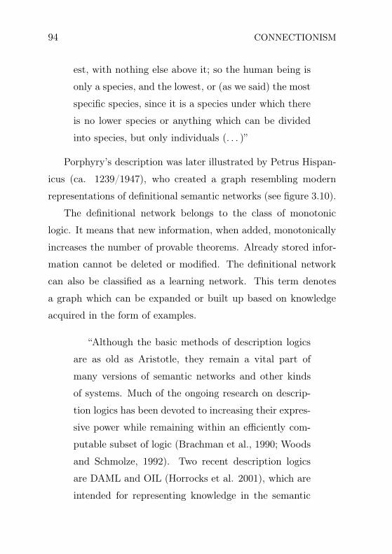
94 CONNECTIONISM
est, with nothing else above it; so the human being is
only a species, and the lowest, or (as we said) the most
specific species, since it is a species under which there
is no lower species or anything which can be divided
into species, but only individuals (. . . )”
Porphyry’s description was later illustrated by Petrus Hispan-
icus (ca. 1239/1947), who created a graph resembling modern
representations of definitional semantic networks (see figure 3.10).
The definitional network belongs to the class of monotonic
logic. It means that new information, when added, monotonically
increases the number of provable theorems. Already stored infor-
mation cannot be deleted or modified. The definitional network
can also be classified as a learning network. This term denotes
a graph which can be expanded or built up based on knowledge
acquired in the form of examples.
“Although the basic methods of description logics
are as old as Aristotle, they remain a vital part of
many versions of semantic networks and other kinds
of systems. Much of the ongoing research on descrip-
tion logics has been devoted to increasing their expres-
sive power while remaining within an efficiently com-
putable subset of logic (Brachman et al., 1990; Woods
and Schmolze, 1992). Two recent description logics
are DAML and OIL (Horrocks et al. 2001), which are
intended for representing knowledge in the semantic
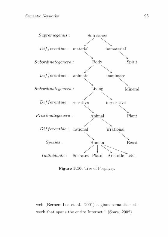
Semantic Networks 95
Supremegenus : Substance
||yyyy
yyy
##HHHHHHH
Differentiae : material
""EEEE
EEE immaterial
""EEEEEE
Subordinategenera : Body
||yyyy
yyy
##HHHHH
HHSpirit
Differentiae : animate
""EEEE
EEE inanimate
""EEEE
EEE
Subordinategenera : Living
||yyyy
yyy
##HHHHH
HHMineral
Differentiae : sensitive
""EEEE
EEE insensitive
""EEEE
EEE
Proximategenera : Animal
||yyyy
yyy
##HHHHHHH Plant
Differentiae : rational
""EEEE
EEE irrational
""EEEE
EEE
Species : Human
||xxxx
xxx
$$IIIIIII
))SSSSSSSSSSSSS Beast
Individuals : Socrates Plato Aristotle etc.
Figure 3.10: Tree of Porphyry.
web (Berners-Lee et al. 2001) a giant semantic net-
work that spans the entire Internet.” (Sowa, 2002)

96 CONNECTIONISM
Apart from definitional networks, many other kinds of seman-
tic networks exist, each expressing a different relation, like, for
example:
• meronymy (A is part of B),
• holonymy (B has A as a part of itself),
• hypernymy (A is superordinate of B) — in some sense, a
reversal of the definitional network,
• synonymy (A denotes the same as B),
• antonymy (A denotes the opposite of B).
It is also possible to introduce more than one relation in a
single semantic network. In this case, edges become labels, which
denote their meaning (figure 3.11).
The other types of semantic networks have, however, little
relevance for this work, and thus will not be further described
here.
Modern Applications
The definitional networks build a core for all common hierarchies
used to define relations of concepts. The first applications of those
networks were done in 1960s and used to define concept types and
relations for machine translation systems (Ceccato, 1961; Master-
man, 1962). The Masterman’s network, in which concepts were
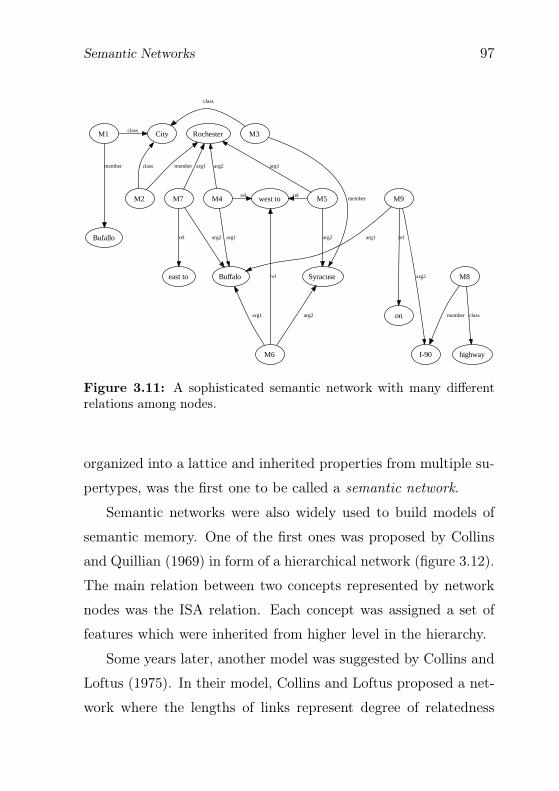
Semantic Networks 97
M1 Cityclass
Bufallo
member
Rochester M3
class
Syracuse
memberM7
arg1
Buffalo
arg2
east to
rel
M2
class member
M4
arg2
arg1
west torel
M5
arg1
arg2
rel
I-90 highwayM6
arg1 arg2
rel M8
member class
M9
arg1
arg2
on
rel
Figure 3.11: A sophisticated semantic network with many differentrelations among nodes.
organized into a lattice and inherited properties from multiple su-
pertypes, was the first one to be called a semantic network.
Semantic networks were also widely used to build models of
semantic memory. One of the first ones was proposed by Collins
and Quillian (1969) in form of a hierarchical network (figure 3.12).
The main relation between two concepts represented by network
nodes was the ISA relation. Each concept was assigned a set of
features which were inherited from higher level in the hierarchy.
Some years later, another model was suggested by Collins and
Loftus (1975). In their model, Collins and Loftus proposed a net-
work where the lengths of links represent degree of relatedness

98 CONNECTIONISM
Figure 3.12: Hierarchical semantic memory model by Collins and Quil-lian (1969).
(figure 3.13). They also introduced the spreading activation pro-
cess, in which the activation of one of the links lead to partial ac-
tivation of connected nodes. To model the relatedness, the search
time was dependent on link length and the degree of activation
decreased with the distance.
Anderson (Anderson and Bower, 1973; Anderson, 1983) pro-
posed a slightly different approach. Knowledge was still repre-
sented in networks, but connections were in the form of propo-
sitions, or statements of relations (propositional network models,
figure 3.14). The model was capable of processing both declarative
knowledge (represented in the model by propositional networks)
and procedural knowledge (represented by production rules). Pro-
duction was effected by interpreting of the propositional network.

Semantic Networks 99
Figure 3.13: Spreading activation network in the tradition of Collinsand Loftus (from Collins and Loftus, 1975, p. 412).
Modern semantic networks are based usually on a network de-
veloped by Woods (1975) and implemented by Brachman (1979)
in a system called KL-ONE: Knowledge Language One. KL-ONE

100 CONNECTIONISM
Office location Frontrelation
Z
subject
Bill
X
word
location
Y
subject
Park relation
agent
ProfessorJones
word
object
BOUGHT
relation
Zagent
OWN
relation
object
Chevy
isa
Fred
word
Car
isa
subject Old
relation
Figure 3.14: A propositional network representing a structure on thesentence level.
is a frame-language,2 which has been developed from Frame Rep-
resentation Language and Knowledge Representation Language.
As an additional feature, in comparison to its ancestors, KL-ONE
introduced constraints involving more than one slot.
“KL-ONE is intended to represent general concep-
tual information and is typically used in the construc-
tion of the knowledge base of a single reasoning entity.
A KL-ONE knowledge base can be thought of as rep-
2Frame-language is a meta-language, where objects are represented byframes, which are collections of named slots that describe types of objectsand relations to other objects. The frames are organized hierarchically.
Semantic Networks 101
resenting the beliefs of the system using it. Thus KL-
ONE fits squarely into the currently prevailing philos-
ophy for building reasoning systems. (. . . )
In other words, KL-ONE provides a language for
expressing an explicit set of beliefs for a rational agent.”
(Brachman and Schmolze, 1985, p. 174)
Figure 3.15: A simple KL-ONE network of generic concepts (fromBrachman and Schmolze, 1985, p. 180).
KL-ONE can be used to represent a full range of semantical
relationships, from simple objects hierarchy (figure 3.15) to elab-
orated semantical dependencies (figure 3.16).

102 CONNECTIONISM
Figure 3.16: A network representing a sentence in KL-ONE (fromBrachman and Schmolze, 1985, p. 214).
3.7 Connectionism vs. Brain Structure
It is often claimed that connectionist models (especially those of
the PDP kind) are derived from the structure of brain. Indeed,
in such models there are nodes and connections, where nodes are
interpreted as a parallel to neurons. However, it should be noted
that this is actually the only relation between connectionist models
(artificial neural networks) and brains (real neural networks).
There are several reasons why connectionist models are not

Connectionism vs. Brain Structure 103
Figure 3.17: A neuron: the major structural and functional “unit” ofnervous tissue.
analogues to the structure of the brain. First of all one has to note
that nodes in connectionist networks are very simple processing
units while real neurons (figure 3.17), on the contrary, are able to
perform relatively complicated calculations on input signals (c.f.
Koch et al., 1982, 1983; Mel, 1994).
An even more important reason to reject connectionist models
as models of the human brain is just the the underlying concept of
these models. They are only some kind of mathematical paradigm,
some formulation of algorithmic procedures. Parallel distributed
processing models are often called universal approximators, which
means that they are just mathematical tools able to approximate
(almost) any arbitrary kind of relation between two sets of num-
bers. Localist models are usually used to approximate even more
abstract cognitive processes. There is no, or very little, attention
paid to simulating how the brain really deals with the tasks in

104 CONNECTIONISM
question. Connectionism just a tries to model the task itself. The
above is mentioned by Krebs (2005) as a clash between top-down
psychological models and bottom-up neural environments. Thus
“(. . . ) when simple ANNs [artificial neural networks]
with small numbers of nodes are employed to model
complex high level cognitive functions, the experimen-
ter should evaluate whether the simplicity of the net-
work can provide a plausible implementation, because
it is all too easy to provide a neurologically possible
model.” (Krebs, 2005, p. 1189)
3.8 Connectionism and Language Processing
The most widely spread approach to natural language processing
and understanding is based on sets of rules and representations.
The connectionist paradigm contrasts with this approach in that
it is based upon sets of nodes and connections, which are described
with vectors and matrices as well as complex apparatus to transfer
information between nodes (like spreading activation mechanism).
There are two different strategies which represent linguistic
phenomena within connectionist theory: model-centered and prin-
ciple-centered.
“[M]odel-centered strategy proceeds as follows (. . . ):
specific data illustrating some interesting linguistic phe-
nomena are identified; certain general connectionist
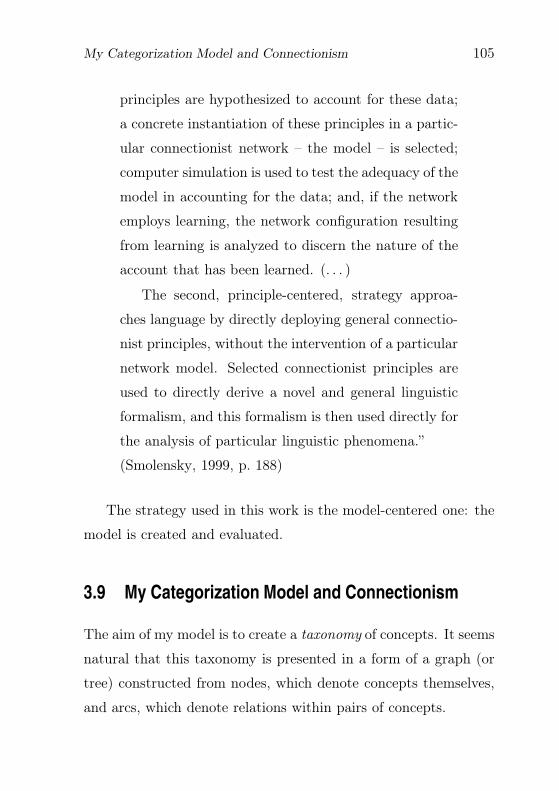
My Categorization Model and Connectionism 105
principles are hypothesized to account for these data;
a concrete instantiation of these principles in a partic-
ular connectionist network – the model – is selected;
computer simulation is used to test the adequacy of the
model in accounting for the data; and, if the network
employs learning, the network configuration resulting
from learning is analyzed to discern the nature of the
account that has been learned. (. . . )
The second, principle-centered, strategy approa-
ches language by directly deploying general connectio-
nist principles, without the intervention of a particular
network model. Selected connectionist principles are
used to directly derive a novel and general linguistic
formalism, and this formalism is then used directly for
the analysis of particular linguistic phenomena.”
(Smolensky, 1999, p. 188)
The strategy used in this work is the model-centered one: the
model is created and evaluated.
3.9 My Categorization Model and Connectionism
The aim of my model is to create a taxonomy of concepts. It seems
natural that this taxonomy is presented in a form of a graph (or
tree) constructed from nodes, which denote concepts themselves,
and arcs, which denote relations within pairs of concepts.
106 CONNECTIONISM
This kind of graph can be classified as a subtype of semantic
networks, namely a definitional network. A taxonomy is noth-
ing else than a definition of ISA relations (cf. definitional net-
works, page 92) between classes of objects (concepts) and their
subclasses. It is obvious that an instance of a given class auto-
matically is an (ISA) instance of its superclass. This simple defi-
nitional network is however enriched with nodes denoting features
of concepts to be classified as well as with interrelations among
those nodes and concepts themselves.
In order to provide more than a purely representational power,
activation spreading and weighted connections are introduced.
These properties make the model presented a part of the class of
“traditional” connectionist systems. Labeled nodes make it rather
a localist connectionist model. However (as will be shown further),
my model, while showing strong localist characteristics, remains
a mixed one.
To summarize: the model presented here is a connectionist
model, displaying several properties of both distributed and lo-
calist approaches to connectionism. It contributes to the class of
connectionist systems able to learn as well as those which perform.
At the same time my model can be seen as a means for building
a “living” taxonomy, a kind of a semantic network.
In the next chapter, the connectionist system able to create hier-
archy of concepts is presented and evaluated.

Part II
Practice


CHAPTER 4
Architecture and Operation of the Model
The description of the model’s operation as well as its internal
architecture are presented in this chapter. The system presented
falls into the class of connectionist models (chapter 3, page 63).
Since the model is connectionist, its main constituent is a net-
work. The basic elements of this network are nodes. The struc-
ture of nodes is inspired by biological findings concerning signal
processing in brain. (It must be noted, however, that the pur-
pose of the system is not to model the architecture or function-
ality of the brain itself, but the higher cognitive ability: the cat-
egorization process.) Consequently, the signal flow in a network
constructed from those structured nodes must undergo a proce-
109

110 ARCHITECTURE AND OPERATION OF THE MODEL
dure that fits this architecture: this is the activation spreading
mechanism, which takes care of transferring information within a
network in general and within this model in particular.
4.1 A Node
In “traditional” connectionist systems (e.g. McClelland and Rumel-
hart, 1981), a node is a simple unit capable of performing basic
operations on incoming signals. The state of such a node is defined
by a given mathematical function, called an activation function,
where the number of arguments is defined by the number of in-
coming connections. Several classes of activation functions are in
use, among them: sigmoidal (logistic) functions (cf. McCullagh
and Nelder, 1989; Jordan, 1995) for feed-forward networks in the
PDP tradition; winner-take-all (cf. Schmutz and Banzhaf, 1992);
different kinds of radial functions (cf. Broomhead and Lowe, 1988;
Moody and Darken, 1989); self-organizing maps (Kohonen, 1982);
and many other kinds dependent on the structure and function-
ality of the network. Nevertheless, the general characteristics of
nodes in typical connectionist systems are that they do not have
any sophisticated internal structure, and do not process incoming
signals in a more elaborate manner.
In contrast to the above, the operation principle of each single
node within my model is based on the finding that neurons are
divided into subregions which are able to perform complex com-

A Node 111
putations on incoming signals (c.f. Koch et al., 1982, 1983; Mel,
1994).
“When two neighboring regions of a dendritic tree ex-
perience simultaneous conductance changes — induced
by synaptic inputs — the resulting postsynaptic po-
tential at the soma is usually not the sum of the po-
tentials generates by each synapse alone. (. . . ) [I]t has
been customary to assume linear summation of exci-
tatory and inhibitory inputs on the dendrites and to
regard the thresholds associated with spike generation
at the axon hillock as performing the elementary log-
ical operations in the nervous system. It is, however,
possible that synapses situated close to each other on
the dendrite of a cell may interact in a highly nonlinear
way.” (Koch et al., 1983, p. 2799)
“One of the question of greatest interest in the study
of neuronal information processing regards the limit of
the computational power of the single neuron. In this
vein, the (. . . ) idea we consider here is that nonlinear
membrane mechanisms, if appropriately deployed in
a dendritic tree, can allow single neuron to act as a
powerful multilayer computational network.”
(Mel, 1994, p. 1065)
While a single real neuron can be seen as analogous to the
whole “classical” distributed connectionist network, it is justified
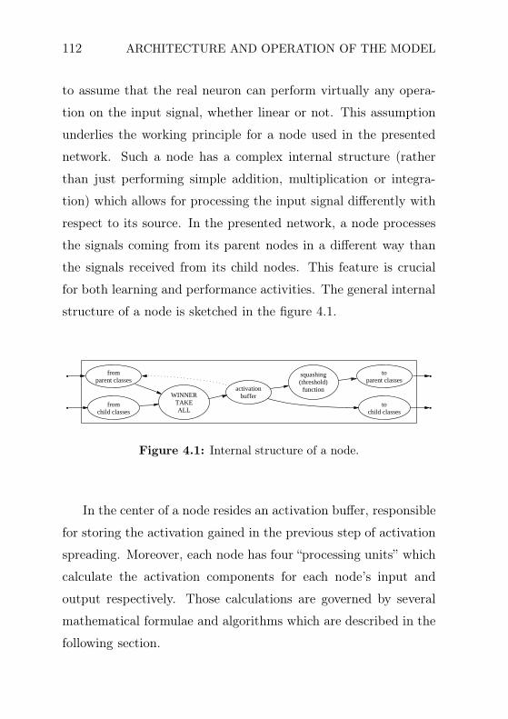
112 ARCHITECTURE AND OPERATION OF THE MODEL
to assume that the real neuron can perform virtually any opera-
tion on the input signal, whether linear or not. This assumption
underlies the working principle for a node used in the presented
network. Such a node has a complex internal structure (rather
than just performing simple addition, multiplication or integra-
tion) which allows for processing the input signal differently with
respect to its source. In the presented network, a node processes
the signals coming from its parent nodes in a different way than
the signals received from its child nodes. This feature is crucial
for both learning and performance activities. The general internal
structure of a node is sketched in the figure 4.1.
fromparent classes
fromchild classes
WINNERTAKEALL
activationbuffer
squashing(threshold)
function
tochild classes
toparent classes
Figure 4.1: Internal structure of a node.
In the center of a node resides an activation buffer, responsible
for storing the activation gained in the previous step of activation
spreading. Moreover, each node has four “processing units” which
calculate the activation components for each node’s input and
output respectively. Those calculations are governed by several
mathematical formulae and algorithms which are described in the
following section.
Activation Spreading 113
4.2 Activation Spreading
The term activation is used here as an abbreviation for a node’s
activation value. It describes a state of a node. The activation is
also a means for transferring information along connections from
one node to another. Its current value is, roughly speaking, a func-
tion of its previous activation and of the state of the remaining
network. It behaves, however, locally: only the nearest neighbor-
hood influences the node in question. The more remote parts of
the network affect it only indirectly.
The activation spreading mechanism is closely connected to
the internal structure of the node. It also differentiates between
signals coming from parent and child nodes as well as between
outgoing signals.
There are four components which contribute to the activation
value: input from parent nodes, input from child nodes, inhibition
and the previous activation of the given node.
4.2.1 Signals from Parent Nodes.
Nodes’ Phase Space and Attractors
The idea of the nodes’ phase space is taken from physics.
phase space — (physics) an ideal space in which the
coordinate dimensions represent the variables that are

114 ARCHITECTURE AND OPERATION OF THE MODEL
required to describe a system or substance; “a multi-
dimensional phase space”.1
For a given node, each connection to a parent node is represented
as an axis in a multidimensional space. In this space a node
is placed in a point characterized by a combination of values of
parent nodes’ activations for which the node in question should
also be activated. Figure 4.2 provides a simple two dimensional
example of two nodes in a phase space.
a bnode 1 0.25 0.75node 2 0.75 0.25
0
0.2
0.4
0.6
0.8
1
0 0.2 0.4 0.6 0.8 1
⊙
⊙
a
b
Figure 4.2: Two sample nodes in 2D phase space.
The phase space mechanism makes it easy to estimate how
much the stimulus provided to the system differs from the one
already coded as a node. Each node constitutes a center in a
phase space relative to which the signals may be examined. The
similarity between stimuli provided and those saved as points in
phase space can be measured in terms of Euclidean distance.
1From http://www.thefreedictionary.com/

Activation Spreading 115
The node’s role in the network’s phase space can be explained
in terms of attractors.
“Let M be a smooth compact manifold, possibly with
boundary, and let f be a continuous map from M into
itself. The notation fn = f . . . f will stand for the
nth iterate of f . Recall that the omega limit set ω(x)
of a point x ∈ M is the collection of all accumulation
points for the sequence x, f(x), f2(x), . . . of successive
images of x. If we choose some metric for the topolog-
ical space M , then ω(x) can also be described as the
smallest closed set S such that the distance from fn(x)
to the nearest point of S tends to zero as n → ∞. The
definition of omega limit set in the case of a continuous
flow on M is completely analogous. Note that ω(x) is
always closed and nonvacuous, with f(ω(x)) = ω(x).
Furthermore, ω(x) is always contained in the nonwan-
dering set Ω(f).
Choose some measure µ on M which is equivalent to
Lebesgue measure when restricted to any coordinate
neighborhood. This can be constructed using a parti-
tion of unity, or using the volume form associated with
a Riemannian metric. It doesn’t really matter which
particular measure we use, since we will usually only
distinguish between sets of measure zero and sets of
positive measure.
116 ARCHITECTURE AND OPERATION OF THE MODEL
Definition. A closed subset A ⊂ M will be called an
attractor if it satisfies two conditions:
1. the realm of attraction ρ(A) consisting of all points
x ∈ M for which ω(x) ⊂ A, must have strictly
positive measure; and
2. there is no strictly smaller closed set A′ ⊂ A so
that ρ(A′) coincides with ρ(A) up to a set of mea-
sure zero.
The first condition says that there is some positive pos-
sibility that a randomly chosen point will be attracted
to A, and the second says that every part of A plays
an essential role.” (Milnor, 1985, p. 179)
In other words, in dynamical systems, an attractor is a set of
values to which the system evolves after a long enough time. For
the set to be an attractor, trajectories that get close enough to
the attractor must remain close even if slightly disturbed. The
connectionist network presented here is a dynamical system be-
cause its state is time-dependent. The nodes (actually the set of
weights of the input connections) play a role of attractors. When
the system receives a set of input values they define a point in
system’s phase space. This point’s coordinates change with the
time and migrate in the direction of the nearest point defined by a
already existing node. In this sense the network acts as an attrac-
tor network. In the case there is no attractor in the neigborhood
Activation Spreading 117
of the initial point, its location in phasespace remains virtually
unchanged.
Overview
Signals coming from parent nodes are processed in a way similar
to calculating a distance in the multi-dimensional phase space.
The number of dimensions is defined by the number of incoming
connections. Additionally, the weights of those connections set
up a point in this space. The node is then able to calculate the
Euclidean distance between the point representing the incoming
signal (defined by activations of parent nodes connected to it)
and the point set up by the weight values. Finally, an activation
function is applied which calculates the activation coming from
parent nodes based on current input signal and the node’s previous
activation (cf. the reciprocal dotted link which originates from
activation buffer in the figure 4.1).
The resulting part of activation coming from parent nodes ex-
presses the difference between the incoming signal and a signal
to which a node is most sensitive, as well as a kind of history of
previous input signals.
Mathematics
The multidimensional space is defined by incoming connections:
their number sets the number of dimensions. Additionally, the
weights of those connections set up a point in this phase space.

118 ARCHITECTURE AND OPERATION OF THE MODEL
The node i calculates the Euclidean distance di between the point
representing the incoming signal (defined by activations aj of par-
ent nodes connected to it) and the point set up by weight values
wji of connections coming into node i. Then a Gaussian function
of this distance is computed:
inpi (t + 1) = e
−d2i
2r2 (4.1)
di =
√∑
j
(wji − aj(t))2 (4.2)
where wji denotes connection strength and aj activation; r is con-
stant and t represents discrete time. The parameter r in the
Gaussian function controls how much the activation function is
“blurred”: the smaller its value, the sharper the activation func-
tion (cf. figure 4.3).
0 1 2 3−1−2−3−4
0.25
0.50
0.75
x
y
y = C(r)e−x
2
2r2
Figure 4.3: Example Gaussian functions: solid line with r = 0.5,dashed line with r = 1.0

Activation Spreading 119
Parameter r controls the network’s sensitivity to the difference
between data stored and new data which constitutes the current
input. The higher the r value is, the less sensitive the network is
to this difference. This parameter allows for modeling behaviors
of different people, who react differently to the slight changes in
stimuli.
Finally an activation function is applied which calculates the
activation coming from parent nodes based on current input signal
and the node’s previous activation:
inpi (t + 1) =
ai(t)(1 − γ) + in
pi (t)(1 − ai(t)) for in
pi (t) ≥ 0
ai(t)(1 − γ) + inpi (t)ai(t) for in
pi (t) < 0
(4.3)
In this formula, γ is constant and describes activation decay
in time. Naturally, the activation value should remain bounded
in a range 0 ≤ ai ≤ amaxi . In this case, amax
i = 1 for all i. The
activation function is chosen in such a way that the resulting part
of activation coming from parent nodes indeed remains bounded
in the desired range. If the final activation value in the previous
step ai(t) is close to the range bounds, the change in the current
step is smaller than for a final activation value lying in the middle
of the range, due to the factors 1 − ai(t) and ai(t) respectively,
which weight the incoming activation inpi (t). Moreover, if the
activation value transgresses the bounds and falls out of the given
range 0 ≤ ai ≤ 1, it will be pulled back into this range in the next

120 ARCHITECTURE AND OPERATION OF THE MODEL
step.
4.2.2 Signals from Child Nodes
Signals from child nodes are calculated simply as the arithmetic
mean of the child nodes’ activations weighted by connection strengths.
inci(t + 1) =
1
N
N∑
j
aj(t)wji (4.4)
The weights wji are connection strengths.
The motivation is as follows. Child nodes j denote subcat-
egories or exemplars of categories defined by a given main node
i. Thus, the most important information is how well, on average,
the category is represented by the data currently processed by
the network. For this purpose, the arithmetic mean is well suited
as it gives the average activation for nodes j which represent the
category in question.
4.2.3 Final Activation Function
The activation components coming from parent and child nodes
are finally subject to a winner-take-all process. In addition, the
inhibition is subtracted.
ini(t) = max(inci (t), in
pi (t)) − inhi(t) (4.5)
where (winhji is the strength of inhibitory connection):

Activation Spreading 121
inhi(t + 1) =N∑
i
ai(t)winhji (4.6)
The task of inhibitory connections is twofold. On the one
hand, they prevent so-called “overheating”, i.e. uncontrolled rise of
activation values in the network’s nodes. On the other hand, and
even more important for a categorization model, they enhance the
contrast between nodes that do not belong to the same category.
This enhanced difference among exclusive categories is one of the
aspects of cognitive economy (cf. Rosch, 1988).
Further calculations differentiate between connections going
in direction of feature nodes and of class nodes. For connections
going to class nodes a squashing function is applied which keeps
the final value in a range between 0.0 and 1.0. This method is
another mechanism to prevent “overheating”. In the presented
network the following function is applied:
ai(t) =
0 for ini(t) ≤ 0
ini(t) for ini(t) ∈ (0, 1)
1 for ini(t) ≥ 1
(4.7)
For connections going in the direction of feature nodes, a threshold
function is used:
outpi (t) =
0 for ini(t) ≤ θ
ini(t) for ini(t) > θ(4.8)
122 ARCHITECTURE AND OPERATION OF THE MODEL
where θ denotes a threshold value. The threshold function was de-
signed because the feature nodes hold the description of currently
processed object. To change or to adapt this description, the sig-
nal coming from class nodes must be strong enough, thus ensuring
that the object was recognized or categorized well enough. If too
low signal levels could influence the state of feature nodes, the
characteristics of categorized objects would be too unstable to be
processed correctly.
4.2.4 Implementation
The implementation of the spreading activation mechanism, which
is a central part of the network algorithm is presented with more
technical details in appendix A, page 223.
4.3 Connections
The connections between nodes are bidirectional and symmetric
with respect to weights. However, they are treated asymmetrically
with respect to activation flow: the activation from parent to child
nodes flows without restrictions but not the other way round. A
child node’s activation influences a parent node’s only in case it
transgresses some given threshold. This is designed because child
nodes have richer featural characteristics which makes them more
sensitive to errors. That is why child nodes need to gain more
activation before they are able to modify the activation of their
superclasses. This mechanism corresponds to the fact that the
Learning 123
activation flow must be stable enough to change the activation
pattern in higher layers of the network.
In the case that the incoming activation pattern for a child
node is close enough to the one already learned by the network,
the activation mechanism ensures that a given node reaches the
threshold immediately and can also influence its parent nodes.
4.4 Learning
One of the unique features of this semi-localist architecture is its
ability to learn. In principle, there is no sufficient definition for
learning.
“The problem is that learning is such a vast topic; it af-
fects almost everything we do – from learning to tie our
shoelaces when we are young to studying chemistry at
college or learning how to make friends.” (Lieberman,
1992, p. 32)
Very roughly it can be said that learning involves a change in an
organism’s capacities or behavior brought about by experience. In
the case of this connectionist system, learning simply means the
ability to store additional data and to restructure the network in
a way to reflect dependencies between known facts.
The presented network incorporates the unsupervised method
of learning. In the unsupervised learning there is no predefined
correct output state for the network. The networks has to adapt to

124 ARCHITECTURE AND OPERATION OF THE MODEL
a combination of input patterns. There are two most important
kinds of unsupervised leadning methods: Hebbian learning and
competitive learning. In the first method learning is determined
by correlations in activation patterns (Hebb, 1949). In the former
case, the central part of learning algorithm is a unit with the high-
est activation level (for example like in SOM’s; Kohonen, 1982).
In the presented model, the learning proceeds in a Hebbinal-like
style: connections are created and weights are adjusted without
comparison to a set of target outputs but only on the base of
analysis of correlations in activation patterns.
Three kinds of learning (cf. Sowa, 2002) are used.
Rote learning (storing data in the structure of network). This
kind of learning is used to store input data in the network.
It is comparable to long-term memory. Rote learning, in
its principal form, is basically just memorization. It avoids
going into details of presented data and acts without under-
standing the relationships involved in the data.
In principle, rote learning is connected with memorization
by repetition. In this case, however, no repetition is involved
and the data is memorized instantly after it is presented.
Connection weight changes. Changes in connection weights are
a means to create the working structure of the network:
the taxonomy itself. The changes in connection weights are
the most common way of training any connectionist sys-
tem. Especially in systems created in the PDP tradition (cf.

Learning 125
Rumelhart et al., 1986b), this is actually the only sensible
way of learning because in these systems the whole knowl-
edge is represented by sets of weights. In my connectionist
model, unlike in PDP systems, the change of weights is only
one of three learning methods: knowledge is stored not only
in links and their strengths but also in nodes themselves.
Restructuring takes place also in the development of the taxon-
omy. It is done by creating nodes and connections as well as
removing connections. The newly added nodes denote tax-
onomy classes and the links denote relations between each
pair of classes. The restructuring can be seen as an aspect
of constructivism:
“Constructivism models incorporate the principle
of nonstationarity, a principle that in theory of au-
tomata refers to a system’s ability to make changes
to its underlying mechanisms. (. . . ) [T]he cen-
tral component of the constructivist model is that
it does not involve a search through a priori de-
fined hypothesis space, and so is not an instance of
model-based estimation, or paramteric regression.
Instead, the constructivist learner builds this hy-
pothesis space as it learns, and so is characterized
as a process of activity-dependent construction
of the presentations that are to underlie mature
skills.” (Quartz and Sejnowski, 1997)

126 ARCHITECTURE AND OPERATION OF THE MODEL
Restructuring is the most powerful method of learning ap-
plied in the system in question. It allows for memorizing new
data by adding nodes, for generalization from the memorized
facts as well as for creating the taxonomical structure itself.
Despite the fact that the above-mentioned learning methods
are different, they all have a common characteristic, one which
is desirable for learning within connectionist models. Ellis and
Humphreys (1999) define this characteristic as follows:
“An important feature of all the various learning pro-
cedures is that they depend only on local information,
for instance the activations of the units at either end
of the connection, rather than any global property of
the network or distant parts of it.” (p. 654)
4.4.1 Concept Learning
Concepts as constituents of semantic networks were introduced in
Section 3.6.1, page 90. In the following the application of this idea
to the presented model is explained.
“Psychologists use the term concept formation, or
concept learning, to refer to the development of the
ability to respond to common features of categories
of objects or events. Concepts are mental categories
for objects, events, or ideas that have a common set
of features. Concepts allow us to classify objects and

Learning 127
events. In learning a concept, you must focus on the
relevant features and ignore those that are irrelevant.”
(Pettijohn, 1998, p. 191)
In principle, the concept of “concepts” allows for grouping
things according to their functionalities or common features, not
to focus on the individual items. Thus, the concept formation is
very close to the categorization or generalization task.
In machine learning jargon, the learning method leading to the
formation of a network within the model presented here could be
called “concept learning”.
“[A] concept is exemplified by a set of positive exam-
ples (cases that are examples of a concept) and a set
of negative examples (cases that are not examples of
the concept). In concept learning, the learner is at-
tempting to construct a rule or algorithm that allows
it co completely separate the positive and negative ex-
amples.” (Raynor, 1999, p. 59)
In the presented model, a positive example is embodied by features
describing an instance of the class in question, while all instances
of other classes together with their classification constitute the
pool of negative examples. The creation of taxonomical structure
as well as of inhibitory connections ensures the maximal separation
of concepts (classes).

128 ARCHITECTURE AND OPERATION OF THE MODEL
4.4.2 Introspective Processes
The introspection phenomenon may be defined as the direct ob-
servation of one’s own mind and its processes. It was widely intro-
duced to experimental psychology by Wundt (1874). In the orig-
inal sense, Wundt used the term “introspection” („Selbstbeobach-
tung“) to define another source of empirical facts.
“We may add that, fortunately for the science, there
are other [then psychological experiments] sources of
objective psychological knowledge, which become ac-
cessible at the very point which the experimental me-
thod fails us. These are certain products of the com-
mon mental life, in which we may trace the operation
of determinate psychical motives: chief among them
are language, myth and custom.” (Wundt, 1904, p. 5)
“Thus psychology has, like natural science, two ex-
act methods: the experimental method, serving for
the analysis of simpler psychical processes, and the ob-
servation of general mental products, serving for the
investigation of the higher psychical processes and de-
velopments.” (Wundt, 1897, p. 23-24)
The investigation of introspection was rejected as an inplausi-
ble method for general mental processes investigation. However,
there has not been enough serious criticism of introspectionism to
cause its complete rejection (cf. Vermersch, 1999). The process of

Learning 129
introspection can be successfully used in some cases. In particular,
reasoning itself may be described with this method.
Introspection involves only internal memories and assump-
tions. The introspective reasoning could thus be defined as pro-
cessing of already known facts in order to extract relationships
among them. This kind of reasoning thus takes into account only
memories of the presented facts.
The presented connectionist system exploits a kind of an intro-
spection process. At first, only raw facts are directly memorized
without further processing (rote learning) and are stored in a kind
of long-term memory. This action is however not introspective and
serves only to prepare the domain in which future introspective
processes take place.
The proper creation of taxonomy, which aims at extracting the
structure of acquired data, is eventually done by an introspective
process. By means of this process, the network creates a gen-
eral structure of concepts and relations among them based on the
internally stored knowledge. This process involves self-analysis
of the activation flow through the network and incorporates re-
structuring the hierarchy by modifying connections and adding
new nodes (cf. examples in sections 6.1.4, page 144 and 6.1.5,
page 145). During the operation, the network does not refer any
longer to the original input data or any other external resources.
Network’s connections and structure are modified according to
already known facts only, resulting in the fully formed taxonomy.

130 ARCHITECTURE AND OPERATION OF THE MODEL
The connectionist system, based on the mechanisms just pre-
sented has been built and tested against data coming from psy-
chological experiments. The evaluation is described in the next
chapter.

CHAPTER 5
Implementation
Each idea, in order to be used in practice, needs to be imple-
mented. In the case of the connectionist system presented here,
the implementation was realized as a computer program. This
chapter describes the goals of the implementation as well some
design details.
5.1 Objectives
The implementation of the connectionist system in question was
not designed as a production system. Its goal was to provide a tool
131

132 IMPLEMENTATION
to test the behaviour of the system. Thus, it was not optimized
for performance.
The modularity of the network (which is a main component of
the system presented) is reflected in the modularity of the com-
puter program. There are several components defined:
• single nodes,
• connections (excitatory and inhibitory ones),
• the network, and
• tools to process input and output data as well as to produce
the visualization of the network’s current structure.
The network module makes use of node and connections mod-
ules and uses them as building blocks. The whole network also
defines the information flow (spreading activation) which is com-
mon to all network setups. Testing a system creates further addi-
tional demands on the network, like working with different input
data and delivering results in different forms and formats. These
demands were satisfied by custom tools developed to process the
respective data.
5.2 Realization
The Java programming language (in version 1.4.2) was used for im-
plementation (Java Website, 2007). This choice was motivated by
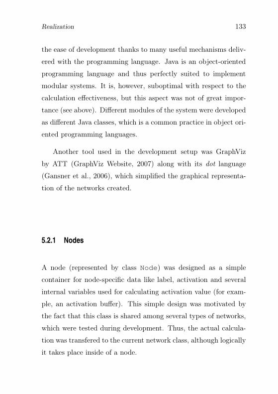
Realization 133
the ease of development thanks to many useful mechanisms deliv-
ered with the programming language. Java is an object-oriented
programming language and thus perfectly suited to implement
modular systems. It is, however, suboptimal with respect to the
calculation effectiveness, but this aspect was not of great impor-
tance (see above). Different modules of the system were developed
as different Java classes, which is a common practice in object ori-
ented programming languages.
Another tool used in the development setup was GraphViz
by ATT (GraphViz Website, 2007) along with its dot language
(Gansner et al., 2006), which simplified the graphical representa-
tion of the networks created.
5.2.1 Nodes
A node (represented by class Node) was designed as a simple
container for node-specific data like label, activation and several
internal variables used for calculating activation value (for exam-
ple, an activation buffer). This simple design was motivated by
the fact that this class is shared among several types of networks,
which were tested during development. Thus, the actual calcula-
tion was transfered to the current network class, although logically
it takes place inside of a node.

134 IMPLEMENTATION
5.2.2 Network
The main component of the implemented system is a Java class,
which represents the network as a whole. The set of nodes, repre-
senting the network was implemented as an array (Java standard
class ArrayList) containing objects of a class Node. All connec-
tions were represented by two-dimensional arrays of real numbers
(with a double precision: double[][]).
To simplify the development, the inheritance property of Java
programming language was used. The basic features of the con-
nectionist system were implemented in a single Net class. This
class contains mainly the spreading activation mechanism, which
doesn’t change along with different usages of the network. Code
snippets which realize the respective tasks, are presented in Ap-
pendix A (page 223) for illustration.
Each of the experiments described in chapter 6 has different
demands with respect to the input data and the expected visual-
ization of the output results. Thus, for each experiment a sepa-
rate Java class was created, which inherited general functionality
from the Net class, but realized the specific input and output
behaviour.
5.2.3 Network visualization
To present the development of the network structure, the GraphViz
tool (GraphViz Website, 2007) was used. This tool is able to draw
graphs, which can be described in one of several different formal
Summary 135
languages. For the purpose of the network visualization the lan-
guge dot (Gansner et al., 2006) was used.
In order to create a dot-compatible description of the network
(for an example see Appendix B, page 227), a class NetPrinter
was created. Its task was to analyze the structure of the data
contained in the object implementing one of the Net subclasses
and to create a text file with the corresponding dot description.
Then the tool from GraphViz package was run automatically to
produce a vector graphic image file in EPS (encapsulated post
script) format. Such created images are used in this work as an
illustration of network structure and operation.
In one experiment – the categorization of ellipses (section 6.1)
– it was necessary to subclass the NetPrinter in order to adapt
the shape of nodes on the output image. The overriden methods
were placed in EllipsePrinter class.
5.3 Summary
The class diagram 5.1 shows the classes used along with the most
important fields and methods. As mentioned before, the detailed
calculations are performed by Java code, which is presented in the
Appendix A.
The system was implemented with use of Borland JBuilder
IDE1 (JBuilder, 2007) version 9.0 Enterprise and tested on the
1IDE — Integrated Development Environment
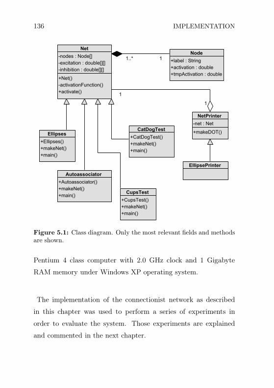
136 IMPLEMENTATION
Figure 5.1: Class diagram. Only the most relevant fields and methodsare shown.
Pentium 4 class computer with 2.0 GHz clock and 1 Gigabyte
RAM memory under Windows XP operating system.
The implementation of the connectionist network as described
in this chapter was used to perform a series of experiments in
order to evaluate the system. Those experiments are explained
and commented in the next chapter.

CHAPTER 6
Evaluation
This chapter presents the results of a series of simulations on the
cognitive properties of the presented model of categorization. The
simulations have been run to evaluate the model. Evaluation here
means two different things. First, there is evaluation of the model
as an IT-system. Second, there is evaluation of the model as a
cognitive model. Both kind of evaluations are discussed in this
chapter.
With respect to the evaluation of the model as IT-system, the
simulations have to illustrate that the model can handle the tasks
it has been designed for. The tasks in question are “creating a tax-
onomy” out of a set of item descriptions (section 6.1), “autoasso-
137

138 EVALUATION
ciation” (section 6.2), and generalization (section 6.3). These sec-
tions concentrate on the proof-of-concept aspect of the IT-system
evaluation. An example is given for every task, such that the
reader gets a good idea how the model solves the tasks. In order
to evaluate a system like the model at hand as an IT-system one
has to run additional tests (Liggesmeyer, 2002; Schmitt, 2003),
such as tests with broken input data. Although some of these
kinds of tests had been performed to obtain the model run, they
are not discussed here since they do not provide any further in-
sights. The bottom line is the model is usable if it can perform
the tasks mentioned successfully.
With respect to evaluating the model as a cognitive model, one
has to check whether its task performance exhibits a behaviour
that is in accordance with the behaviour that subjects exhibit
in psychological experiments. In order to evaluate the model at
hand as a cognitive one, two experiments have been run, one for
fuzzy categorization (section 6.4) and one for asymmetric category
formation (section 6.5). It is to be noted that fuzzy categoriza-
tion has not been a property of the model from the functional
(IT) view of it. Fuzzy categorization has not been implemented
into the model. So, it is interesting how the model reacts under
this question. The idea here is the following: the performance of
the model is compared to the results of psychological experiments,
namely those by Labov (1974). The question is whether the model
passes this test in the sense of Popper’s 1935/1994 “Bewährung”

Introductory Simulation: Creating a Taxonomy 139
(Gadenne, 1998, cf.). The same holds for asymmetric category
formation. Here, the behaviour is compared to an experiment by
(Quinn, 2002). In this case, the model’s behaviour can be at-
tributed to the statistical distribution of features of stimuli that
infants were exposed to. The experiment on asymmetric category
formation therefore provides some support for explanation of the
effect given by Mareschal et al. (2000) and offers additional in-
sight how the effect can be explained in detail. In summary, with
respect to evaluation as a cognitive model, the model is success-
ful if its behaviour is similar to human behaviour as exhibited in
psychological experiments, and if the model provides additional
insights about the reasons behind the human behaviour.
6.1 Introductory Simulation: Creating a Taxonomy
This section describes step-by-step a general routine for creating
a taxonomy with the use of the presented network and illustrates
it through examples. Creating a taxonomy is the very first step
which must be performed before any other properties of the net-
work can be used. Since the network itself forms a taxonomy, it
means also creating a structure of the network.
6.1.1 Training Data
The network operates on data which consists of sets of features
weighted by real numbers. The weights express the degree to
which the respective feature is present in the class’s definition.

140 EVALUATION
This is however not the degree of importance of the feature. For
example, in the case of color, coded as a mix of red, green and blue
components, the weights for the respective basic colors express
only in what ratios they are mixed and not which one is more or
less important.
The features can be chosen arbitrarily. The concrete set of
used weights and values is task-dependent. The network’s pro-
cessing mechanism allows for use of both binary and real valued
weights. The choice between those two types in the following pre-
sented experiments and examples is thus arbitrary, and made only
to keep the examples as easy as possible to interpret.
Example. To investigate the process of creating a network a sim-
ple example with a single real valued feature will be used. The ex-
ample illustrates the categorization of ellipses defined by a ratio of
their semimajor axis to the semiminor axis. Table 6.1 presents the
data used within the example. In the dataset there are two “hori-
zontal” ellipses (i.e., with horizontal semiaxis longer than vertical
one): ellipse_3 and ellipse_4; three ellipses very close in shape
to a circle (ellipse_2, ellipse_5 and ellipse_6) and two “vertical”
ones (i.e., with vertical semiaxis longer): ellipse_0 and ellipse_1.
6.1.2 Storing the Data
In the first step the presented data is memorized only (stored).
This is done by rote learning (cf. section 4.4, page 123). Because

Introductory Simulation: Creating a Taxonomy 141
object ratioellipse_0 2.0ellipse_1 1.95ellipse_2 1.15ellipse_3 0.5ellipse_4 0.55ellipse_5 1.0ellipse_6 0.95
Table 6.1: Data for introductory simulation.
of the local characteristics of the data representation used, the net-
work must be expanded to store new knowledge. Thus, for each
dataset, feature nodes are created as necessary. Additionally, class
nodes are created denoting the respective set of all co-occurring
features. Because the features are characterized not only by their
presence but also by a degree of this presence (value), the features
are said to co-occur only when their values equal within a given
precision. Between class nodes and feature nodes excitatory con-
nections are created with weights corresponding to the values of
respective features.
The procedure described above constitutes one of the construc-
tivist aspects of the model presented in the current work. When
data is not already represented within the network’s structure, the
network is expanded to deal with the new knowledge.

142 EVALUATION
6.1.3 Creating a Hierarchy
Based on the data stored in already created feature and class
nodes a hierarchy is created. The hierarchy developed in this
phase of learning reflects the relations among items only as far
as this is provided explicitly by the input data. One can assume
that in most cases the structure of the network created after this
step is not the final hierarchy. For example, if only the data
concerning exemplars for one category is presented to the system,
the network’s structure is very flat, usually having no more than
two or three levels.
During the hierarchy build-up, the network undergoes the fol-
lowing procedure. For each pair of class nodes, both nodes are
subsequently activated. The activation is spread to the feature
nodes layer and the activation patterns are compared. If one of
the nodes generates an activation pattern comprised in the other
one’s pattern, it is assumed to be its superclass. For example, let
us assume the following sets of binary features:
Set 1. a, b, c, f, g
Set 2. b, c, d
Set 3. a, f, g
In the above example, Set 1 describes a child node of a node
characterized by Set 3, while Set 2 does not have any direct
relation to the other two.

Introductory Simulation: Creating a Taxonomy 143
This principle is based on the simple assumption that a sub-
class contains all features of its superclass and at least one more,
a distinctive one. The comparison of patterns is performed with a
given precision in order to gather classes characterized by features
which values do not differ significantly. This precision is charac-
terized by a threshold θ; all values falling under θ are treated as
equal.
Example. Figure 6.1 shows the results of storing the data and
creating a hierarchy. The node ELLIPSE denotes just a node
which is defined by a features ratio with some value. As previously
mentioned, because the input data (cf. table 6.1) is not structured
at all, the form of a network reflects no real taxonomical structure
at this point. The network has a relatively flat structure of two
levels only.
ELLIPSES
ellipse_0 ellipse_1 ellipse_2 ellipse_3 ellipse_4 ellipse_5 ellipse_6
Figure 6.1: First step in creating a taxonomy: raw input data pre-sented as a network structure.

144 EVALUATION
6.1.4 Network Pruning
The previously described steps of creating a taxonomy lead to a
network which usually contains superfluous excitatory connections
that do not represent direct class – superclass relations. Because
the hierarchy creation algorithm discovers only category inclusive-
ness relations, it is the case that all subcategories are linked to the
main category even if there are other levels of specifications be-
tween them. For example, a pigeon would be linked to the node
denoting animal category even if there also exists a node for a bird
(cf. 6.2). Those connections are removed by an introspective pro-
cess (cf. section 4.4.2, page 128). This process analyzes the acti-
animal
bird
pigeon duck
Figure 6.2: The illustration of the incorrect class—superclass connec-tion. The dashed arrow denotes the undesired edge.
vation flow between two nodes and compares the activation values
in all node pairs. The comparison drives the decision whether two
nodes remain in direct class—superclass relation or not. Roughly
speaking, nodes are assumed to lie on adjacent taxonomical lev-
els when the activation in the subordinate node comes only from
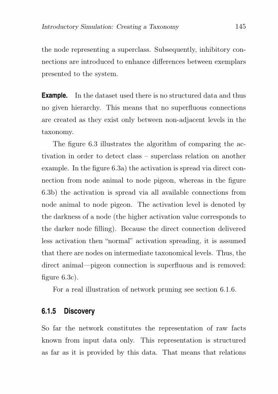
Introductory Simulation: Creating a Taxonomy 145
the node representing a superclass. Subsequently, inhibitory con-
nections are introduced to enhance differences between exemplars
presented to the system.
Example. In the dataset used there is no structured data and thus
no given hierarchy. This means that no superfluous connections
are created as they exist only between non-adjacent levels in the
taxonomy.
The figure 6.3 illustrates the algorithm of comparing the ac-
tivation in order to detect class – superclass relation on another
example. In the figure 6.3a) the activation is spread via direct con-
nection from node animal to node pigeon, whereas in the figure
6.3b) the activation is spread via all available connections from
node animal to node pigeon. The activation level is denoted by
the darkness of a node (the higher activation value corresponds to
the darker node filling). Because the direct connection delivered
less activation then “normal” activation spreading, it is assumed
that there are nodes on intermediate taxonomical levels. Thus, the
direct animal—pigeon connection is superfluous and is removed:
figure 6.3c).
For a real illustration of network pruning see section 6.1.6.
6.1.5 Discovery
So far the network constitutes the representation of raw facts
known from input data only. This representation is structured
as far as it is provided by this data. That means that relations
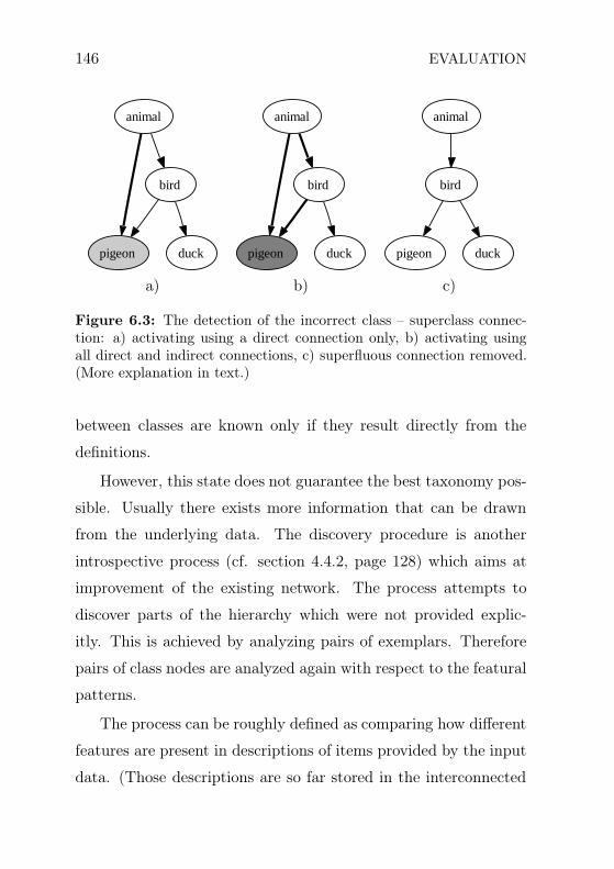
146 EVALUATION
pigeon
animal
bird
duck pigeon
animal
bird
duck
animal
bird
pigeon duck
a) b) c)
Figure 6.3: The detection of the incorrect class – superclass connec-tion: a) activating using a direct connection only, b) activating usingall direct and indirect connections, c) superfluous connection removed.(More explanation in text.)
between classes are known only if they result directly from the
definitions.
However, this state does not guarantee the best taxonomy pos-
sible. Usually there exists more information that can be drawn
from the underlying data. The discovery procedure is another
introspective process (cf. section 4.4.2, page 128) which aims at
improvement of the existing network. The process attempts to
discover parts of the hierarchy which were not provided explic-
itly. This is achieved by analyzing pairs of exemplars. Therefore
pairs of class nodes are analyzed again with respect to the featural
patterns.
The process can be roughly defined as comparing how different
features are present in descriptions of items provided by the input
data. (Those descriptions are so far stored in the interconnected

Introductory Simulation: Creating a Taxonomy 147
net consisting of feature and class nodes.) If the features for two
or more classes overlap (with respect to their presence and value)
they form a description of another class which is assumed to be
a superclass for those currently being analyzed. The description
created thus is presented to the system as new input data.
The generalization process involves, in addition to creating
new descriptions, also their integration into the existing network
structure. To assure correct integration, the new descriptions are
introduced in the exactly same way as the original data. Thus
the problem of superfluous connections described in the previous
section arises once more.
The discovery process is a crucial factor with respect to one of
the most important networks characteristic: generalization. With
respect to this property, it allows for categorization of objects shar-
ing several features common to the objects stored in the network’s
structure during the learning phase.
Example. The network resulting from the discovery of the new
nodes is shown in figure 6.4. Beside nodes already present in
the taxonomy, three new ones are introduced. These new nodes
correspond to the three discovered “classes” of ellipses presented:
one with horizontal axis longer then the vertical axis, one with
both axes almost equal in length and one with vertical axis longer
then the horizontal one. The introduced links connect all nodes
with respect to the class—superclass relation, not necessarily only
those on the adjacent levels of hierarchy.

148 EVALUATION
ELLIPSES
ellipse_0 ellipse_1 ellipse_2 ellipse_3 ellipse_4ellipse_5 ellipse_6
Figure 6.4: The form of a network after the discovery procedure.
6.1.6 Final Network
The network created so far contains nodes representing all terms
which could have been discovered from the presented data. How-
ever, because the data discovered in the previous step was intro-
duced in the same fashion as the original input data, the network
suffers again from many superfluous connections. This is of course
still undesired as it introduces unwanted chaos and destroys the
clear taxonomical structure.
Therefore, the final step in the procedure of creating a taxon-
omy from examples is to clean the network by removing superflu-
ous connections. This pruning is done according to the algorithm
described in section 6.1.4 above.
The resulting connectionist system reflects the taxonomical
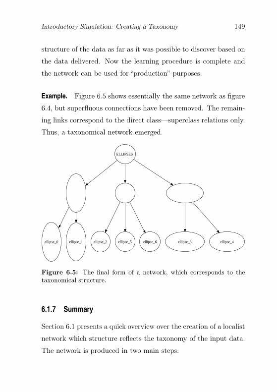
Introductory Simulation: Creating a Taxonomy 149
structure of the data as far as it was possible to discover based on
the data delivered. Now the learning procedure is complete and
the network can be used for “production” purposes.
Example. Figure 6.5 shows essentially the same network as figure
6.4, but superfluous connections have been removed. The remain-
ing links correspond to the direct class—superclass relations only.
Thus, a taxonomical network emerged.
ELLIPSES
ellipse_0 ellipse_1 ellipse_2 ellipse_3 ellipse_4ellipse_5 ellipse_6
Figure 6.5: The final form of a network, which corresponds to thetaxonomical structure.
6.1.7 Summary
Section 6.1 presents a quick overview over the creation of a localist
network which structure reflects the taxonomy of the input data.
The network is produced in two main steps:

150 EVALUATION
• creating a raw network (which depicts only the raw data),
and
• restructuring it (in order to create the full taxonomy that
can be deduced from the presented data).
In the following, experiments and simulations using the finished
network will be described in order to explore its properties and
behavior.
6.2 Introductory Simulation: Autoassociation
The autoassociator in distributed connectionism is a relatively
simple architecture in which the output signal is looped back to
the inputs of network’s nodes. In localist connectionism, however,
the autoassociation property has received little research attention.
This section presents the autoassociation property of the net-
work. Autoassociation is illustrated by an example of binary fea-
tures in order to simplify the exemplification of this process.
6.2.1 Preparing a Network
To investigate the autoassociation property one first needs a com-
plete network. Thus, a network is created according to the proce-
dure described in the previous section.
Example. A network is built from the data presented in table 6.2.
The data describes roughly several types of military equipment.

Introductory Simulation: Autoassociation 151
Objects are defined by several binary features describing their
main characteristics. Of course, the dataset is very simplified in
order not to lose the process overview in the jungle of unnecessary
connections. The resulting taxonomy is presented in figure 6.6a.
object featuresLEOPARD_2 armour tracked selfprop tankJAGUAR_1 armour tracked selfprop antitank hotJAGUAR_2 armour tracked selfprop antitank towFH_70 towed howitzerPzH2000 armour tracked selfprop howitzer
Table 6.2: Data for autoassociation simulation.
6.2.2 Autoassociation Process
The autoassociation property is a special case of pattern associ-
ation and means that a network is able to recover its full state
from partial description of the activation pattern. This feature
of a network can be seen as a kind of long-term memory where
sets of units are associated into patterns which can be recalled on
demand.
The importance of the autoassociation property manifests it-
self in two main topics. One of them is object recognition under
noisy conditions. This means that the network is able to classify
items even if the feature set given as input data is blurred or cor-
rupt, or several features are missing. This ability reinforces the
system operation in environments where available data is distorted
and thus enhances system’s robustness.

152 EVALUATION
LEOPARD_2
JAGUAR_1 JAGUAR_2
FH_70
PzH2000
armour
armourselfproptracked
selfproptank
armourselfprop
tanktracked
trackedantitank
antitankarmourselfproptracked
hot
antitankarmour
hotselfproptracked
tow
antitankarmourselfprop
towtracked
howitzer
howitzertowed
armourhowitzerselfproptracked
towed
Figure 6.6a: Starting network for autoassociation demonstration.
Introductory Simulation: Autoassociation 153
In a more general sense, the autoassociation property means
“noise reduction” and the ability to recognize and recall incomplete
patterns. The property is equivalent to analogous properties in
contemporary models of vision (Ge and Iwata, 2002; Rolls, 2003)
and memory (Rolls and Treves, 1997).
Another application of the autoassociation property is its use
in discovering novel items. In the case that system converges to
a state far from the initial one, the input data can be treated as
novel data (cf. section 6.5, page 169).
Example. The autoassociation procedure is evaluated in this case
as a way to complete the description of an item. In the network
representing data from table 6.2 two feature nodes are activated.
To simplify demonstration, they are chosen to unambiguously de-
fine an item. Thus, the simulation starts with activation of two
feature nodes (cf. figure 6.6b):
• tracked, which is common to most of objects described by
the network and
• hot, which is a distinctive feature of the JAGUAR_1 ob-
ject.
Following thereon, the activation spreading mechanism is used
to transfer the signal between network nodes. The activation pat-
tern in the network changes, and the activation is being trns-
ferred into feature nodes such that the full characteristics of the
JAGUAR_1 are reconstructed (figure 6.6c).

154 EVALUATION
In this way the autoassociation property manifested itself by
associating part of the description (two initially activated nodes)
with the complete characteristics of the item in question.
6.3 Introductory Simulation: Generalization
The generalization term is used to indicate the property of the net-
work which allows it to categorize objects previously not known.
Along with autoassociation, the generalization property is seen as
a strength of connectionist systems. However, it was thoroughly
investigated for systems based on a distributed data representa-
tion (cf. Shekhar and Amin, 1992; Musavi et al., 1994; Chris-
tiansen and Chater, 1994) but again neglected in the case of lo-
calist architectures.
Generalization is especially important for understanding the
phenomena of categorization. Roughly speaking, the most vital
part of the categorization process can be seen as generalizing over
many concrete objects or instances of a given class. Obviously,
this is a common and important property of human categoriza-
tion. People, for example, do not have any problem to categorize
most birds they never saw before as instances of the class bird.
Generally speaking, unknown objects can usually be assigned to
some broader category.
In the model presented, ability to generalize is developed dur-
ing the learning phase. Unlike in the distributed data represen-
tation architectures, the generalization property is not a result of
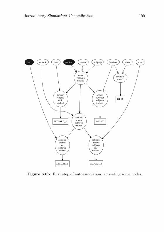
Introductory Simulation: Generalization 155
LEOPARD_2
JAGUAR_1 JAGUAR_2
FH_70
PzH2000
armour
armourselfproptracked
selfproptank
armourselfprop
tanktracked
trackedantitank
antitankarmourselfproptracked
hot
antitankarmour
hotselfproptracked
tow
antitankarmourselfprop
towtracked
howitzer
howitzertowed
armourhowitzerselfproptracked
towed
Figure 6.6b: First step of autoassociation: activating some nodes.

156 EVALUATION
LEOPARD_2
JAGUAR_1 JAGUAR_2
FH_70
PzH2000
armour
armourselfproptracked
selfproptank
armourselfprop
tanktracked
trackedantitank
antitankarmourselfproptracked
hot
antitankarmour
hotselfproptracked
tow
antitankarmourselfprop
towtracked
howitzer
howitzertowed
armourhowitzerselfproptracked
towed
Figure 6.6c: Autoassociation successful: object characteristics are re-stored.
Cup or Bowl: Fuzzy Categorization 157
approximation done with numbers of free parameters (connection
weights). It is a result of the restructuring of the network and
the creation of additional nodes, which carry the characteristics
common to two or more objects presented to the system. Thus
the proposed solution seems to be more robust with respect to
new data introduced (see comments on catastrophic forgetting:
section 7.8.1).
Example. The generalization can be observed if features are ac-
tivated which do not fit together in the description of a known
object. This situation simulates the encounter of unknown exem-
plar, which shares several features common to the ones present in
the training dataset.
Let us assume that, in the example used to illustrate the au-
toassociation property (section 6.2), the feature tow also is ac-
tivated (cf. figure 6.7a). Thus, the network should classify an
unknown object which has the features tracked, hot and tow.
The network converges in this case to the more general term which
could be labelled as antitank vehicle. Thus, the general descrip-
tion for object carrying similar descriptions is activated. The final
state of the network is shown on the figure 6.7b.
6.4 Cup or Bowl: Fuzzy Categorization
Following the series of introductory experiments showing the basic
properties of the presented model, this section describes a simula-
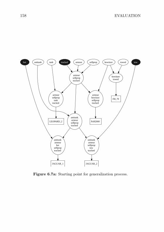
158 EVALUATION
LEOPARD_2
JAGUAR_1 JAGUAR_2
FH_70
PzH2000
armour
armourselfproptracked
selfproptank
armourselfprop
tanktracked
trackedantitank
antitankarmourselfproptracked
hot
antitankarmour
hotselfproptracked
tow
antitankarmourselfprop
towtracked
howitzer
howitzertowed
armourhowitzerselfproptracked
towed
Figure 6.7a: Starting point for generalization process.

Cup or Bowl: Fuzzy Categorization 159
LEOPARD_2
JAGUAR_1 JAGUAR_2
FH_70
PzH2000
armour
armourselfproptracked
selfproptank
armourselfprop
tanktracked
trackedantitank
antitankarmourselfproptracked
hot
antitankarmour
hotselfproptracked
tow
antitankarmourselfprop
towtracked
howitzer
howitzertowed
armourhowitzerselfproptracked
towed
Figure 6.7b: Autoassociation successful in case of contradicting fea-tures: network converges to the more general term, here presented bythe node “antitank, armour, selfprop, tracked”
160 EVALUATION
tion based on the original experiment on boundaries of meanings
of words conducted by Labov.
The aim of the simulation is to compare the behavior of the
network against the experiments performed on human subjects,
and thus to judge whether the model presented here catches se-
lected properties of human cognition.
6.4.1 Original Experiment
The original experiment to be simulated here was described by
Labov (1974). The results presented then shed a new light on
the ideas of categorization of words’ meanings. This was the first
serious series of experiments which gave new insight into the cat-
egorization process. The formation of categories had until then
been not being studied but rather the process had been assumed
and “ready-to-use” categories utilized in the linguistic investiga-
tions.
The aim of this experiment was to investigate the boundaries
between meanings of words rather than meaning itself. While it
is very complicated to analyze the meaning of a single concept,
distinguishing between two of them seems to be relatively simpler
task. From a technical point of view, the act of naming “which
associates a linguistic sign with an element of the extra-linguistic
world” (Labov, 1974, p. 347) was studied. The naming experiment
was based upon a series of drawings of cup-like objects, varying in

Cup or Bowl: Fuzzy Categorization 161
sizes and shapes (cf. figure 6.8). The experiment was conducted
in the following way:
“The drawings of cups are presented to subjects
one at a time, in two different randomized orders; the
subjects are simply asked to name them. They are
then shown the same series of drawings again, and
this time asked to imagine in each case that they saw
someone with the object in his hand, stirring in sugar
with a spoon, and drinking coffee from it (or in some
languages, tea), and to name them in this context.
In a third series, they are asked to imagine that they
came to dinner at someone’s house and saw this object
sitting on the dinner table, filled with mashed potatoes
(rice for some languages). (. . . ) We will refer to these
(. . . ) contexts as the ‘Neutral’, ‘Coffee’, ‘Food’ (. . . )
contexts. (. . . ) The responses to these tests are in
the form of noun phrases, often with a wide range of
modifiers. In our present analysis, we consider only a
head noun.” (Labov, 1974, p. 355)
The above-described procedure was conducted on several do-
zens of subjects and for a wide language spectrum. On the whole,
the investigation of boundaries of meaning took over ten years to
complete.
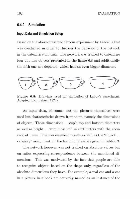
162 EVALUATION
6.4.2 Simulation
Input Data and Simulation Setup
Based on the above-presented famous experiment by Labov, a test
was conducted in order to discover the behavior of the network
in the categorization task. The network was trained to categorize
four cup-like objects presented in the figure 6.8 and additionally
the fifth one not depicted, which had an even bigger diameter.
Figure 6.8: Drawings used for simulation of Labov’s experiment.Adapted from Labov (1974).
As input data, of course, not the pictures themselves were
used but characteristics drawn from them, namely the dimensions
of objects. Those dimensions — cup’s top and bottom diameters
as well as height — were measured in centimeters with the accu-
racy of 1 mm. The measurement results as well as the “object —
category” assignment for the learning phase are given in table 6.3.
The network however was not trained on absolute values but
on ratios expressing correspondence between the mentioned di-
mensions. This was motivated by the fact that people are able
to recognize objects based on the shape only, regardless of the
absolute dimensions they have. For example, a real car and a car
in a picture in a book are correctly named as an instance of the

Cup or Bowl: Fuzzy Categorization 163
a) b)object dimensions
id bottom top height
1 1.0 2.2 1.62 1.7 2.64 1.63 2.2 3.3 1.64 2.7 4.18 1.65 3.0 5.5 1.6
object contextid neutral food1 cup cup2 cup cup3 cup bowl4 bowl bowl5 bowl bowl
Table 6.3: Data used for simulation of Labov’s experiment: a) dimen-sions of objects, b) assigned categories in two contexts.
“car” category, or distant objects which seem to be smaller are as
equally well categorized as those present nearby. This suggests
that it is appropriate or even better grounded to use the relations
between an object’s dimensions, which describe the shape, for the
learning task. The ratios used were bottomtop , height
top and heightbottom .
The training data was organized into vectors containing an id
for the object in question as well as all three above-mentioned
ratio values. (An object’s id is its unique identifier.) For example,
the vector: (1, 5
11, 8
11, 1.6) is a valid input.
In the experiment a set of 500 networks were used. A single
network simulates a subject in the Labov’s experiment. It was
trained on the set of data created as described above. Then con-
nection weights were randomly changed up to a difference of 25%
in value. These changes were meant to correspond to individ-
ual experiences of people: a change in weight means a change in
sensitivity to the stimulus.

164 EVALUATION
Method
For each of the 500 networks with modified weights the following
simulation steps were conducted:
• for each dataset the feature nodes were activated with cor-
responding values, provided as input vector coordinates,
• activation was spread for 100 steps (the step number was
chosen that high to assure a stable final activation pattern),
• the sum of activation of nodes corresponding to learned ex-
emplars was calculated,
• a network was said to categorize an item as a “cup” when
the sum of activation for nodes corresponding to learned cup
objects was higher than the one corresponding to learned
bowl objects, and as a “bowl” otherwise.
For each dataset the cumulative number of categorizations as
“cup” and as “bowl” by all networks was stored separately and
expressed as percentage of overall number of categorization acts.
Complementary Experiments Additionally, three complementary si-
mulations were conducted in order to investigate another property
of the network, namely the priming phenomenon. These addi-
tional simulations were conducted to examine the influence of sit-
uational context as well as of previous categorization on results of
the current one.

Cup or Bowl: Fuzzy Categorization 165
In the first experiment the influence of a context was checked.
An additional feature “context” was introduced (cf. table 6.3b).
It had the meaning of neutral or of food context1.
In two further simulations the networks underwent another
procedure in order to check the influence of previous categorization
act. The system categorized a test object after categorizing either
an object which was a cup or a bowl first.
Results
The results of the categorization experiments are gathered in ta-
bles 6.4 and 6.5 and presented as graphs (figures 6.9 and 6.10).
The resulting data expresses the probability of classifying an ob-
ject as a “cup” or “bowl” against ratio of bottom width of the
object in question to the bottom width of the first object in two
different contexts. This form of presentation is chosen to allow
direct comparison against the results as presented in the original
work (Labov, 1974). The probability is given here as a percent
[%] of the overall number of categorization acts.
For direct comparison the figure 6.11 which presents the origi-
nal results obtained by Labov in 1974 in naming experiment con-
ducted on eleven subjects (cf. subsection 6.4.1) is included here.
1The meaning of a “context” in this case is explained in the quotation onthe page 161.

166 EVALUATION
width categorization probability [%]ratio cup bowl1 100 01.2 100 01.5 73.51247601 26.487523991.9 12.28733459 87.712665412.5 6.862745098 93.1372549
Table 6.4: Results of simulation of Labov’s experiment (neutral con-text).
cup
bowl
1 1.5 2 2.5
0
20
40
60
80
100
width ratio
probability[%]
Figure 6.9: Results of simulation of Labov’s experiment (neutral con-text).
Experiment Discussion
The human categorization process is influenced by numerous fac-
tors. Thus it is not possible to fully simulate it in this simple
simulation. The categorization process bases on much more data

Cup or Bowl: Fuzzy Categorization 167
width categorization probability [%]ratio cup bowl1 100 01.2 62.76803119 37.231968811.5 11.39489194 88.605108061.9 0 1002.5 0 100
Table 6.5: Results of simulation of Labov’s experiment (food context).
cup
bowl
1 1.5 2 2.5
0
20
40
60
80
100
width ratio
probability[%]
Figure 6.10: Results of simulation of Labov’s experiment (food con-text).
and constraints that simple dimension ratios of objects in ques-
tion. However, the qualitative similarities between the results from
the network simulation and the original experiment are obvious.
Both studies show the vagueness of the border between categories
of cups and bowls.
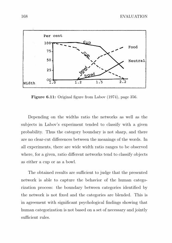
168 EVALUATION
Figure 6.11: Original figure from Labov (1974), page 356.
Depending on the widths ratio the networks as well as the
subjects in Labov’s experiment tended to classify with a given
probability. Thus the category boundary is not sharp, and there
are no clear-cut differences between the meanings of the words. In
all experiments, there are wide width ratio ranges to be observed
where, for a given, ratio different networks tend to classify objects
as either a cup or as a bowl.
The obtained results are sufficient to judge that the presented
network is able to capture the behavior of the human catego-
rization process: the boundary between categories identified by
the network is not fixed and the categories are blended. This is
in agreement with significant psychological findings showing that
human categorization is not based on a set of necessary and jointly
sufficient rules.

Cats Could Be Dogs 169
6.5 Cats Could Be Dogs
This simulation explores the properties of category learning by
infants. It is based on the idea of an experiment presented by
Quinn et al. (1993) which investigates category formation in early
infancy.
6.5.1 Original Experiment
The original series of experiments concerns about the creation of
the representation of perceptually similar categories in the early
infancy, and was presented by Quinn et al. (1993). In one of the
experiments the authors
“(. . . ) explored the ability of infants to differentiate
categorical representations of dogs from specific in-
stances of cats and categorical representations of cats
from specific instances of dogs.” (Quinn et al., 1993,
p. 471)
This test trial showed that the novelty preference scores for in-
fants familiarized with cats was greater than for those familiarized
with dogs. The difference was substantially higher than statisti-
cal effects. One “explanation of this difference lies in a possible
asymmetry in the structure of the two categories” (Quinn et al.,
1993, p. 472).
The following simulation explores the formation of perceptu-
ally similar categories of dogs and cats with use of the connec-

170 EVALUATION
tionist system presented in this paper. The main factor of this
experiment is the investigation of asymmetry in the developed
categories.
6.5.2 Simulation
The simulation was designed to test whether the network is able
to develop a category representation which has the property dis-
covered by Quinn et al.
Input Data and Simulation Setup
Like in the previously described simulation of Labov’s experiment
(section 6.4), the original data in form of pictures obviously could
not be used in the following simulation because the network is not
equipped with any kind of mechanism to analyse pictures directly.
In the simulation made, therefore, the dataset used by Mareschal
et al. (2000) was reused. This data consists of measurements of the
most crucial properties of the original pictures. Table 6.6 shows
the measurements for cat images, table 6.7 for dog images.
Based on the data gathered in tables, vectors were created with
respective measurement values used as components. Those vectors
were then normalized to the unitary length. The normalization
expresses again the fact, that rather the shape, and thus only
relations among different dimensions, is important, and not the
absolute values.

Cats
Could
Be
Dogs
171
head head eye ear ear nose nose leg vertical horizontalexemplar length width separation separation length length width length extent extent
cat1 29 32 7 28 12 0 3 0 54 62cat2 12 13 4 12 5 3 2 14 25 50cat3 20 20 4 17 6 5 3 15 26 67cat4 13 17 4 17 5 3 2 28 28 46cat5 13 14 4 14 4 4 3 15 23 42cat6 18 22 3 17 6 6 3 24 42 70cat7 10 12 3 7 3 2 1 24 24 47cat8 23 24 5 26 7 4 4 25 50 64cat9 16 17 4 15 5 5 4 22 32 54cat10 16 15 3 12 8 3 2 15 30 65cat11 19 27 5 20 8 4 3 22 71 57cat12 19 21 4 12 5 5 4 20 39 65cat13 25 30 6 30 14 6 5 0 50 81cat14 16 20 3 16 13 5 3 26 29 59cat15 17 27 5 22 5 3 3 28 40 43cat16 18 21 4 20 6 4 4 35 55 43cat17 23 22 5 24 7 6 4 35 52 56cat18 20 22 5 23 7 5 4 28 34 54
Table 6.6: Data for cats in “cats and dogs” experiment (sizes in mm).

172
EVA
LU
AT
ION
head head eye ear ear nose nose leg vertical horizontalexemplar length width separation separation length length width length extent extent
dog1 16 22 0 0 16 6 7 25 21 53dog2 23 16 0 2 8 5 8 35 21 42dog3 16 16 4 13 5 7 6 25 26 64dog4 20 24 4 11 7 10 10 29 22 47dog5 15 22 4 0 20 10 6 31 34 55dog6 13 15 3 4 8 6 4 25 19 41dog7 15 20 3 5 9 8 5 28 26 60dog8 13 9 4 12 8 7 5 19 20 49dog9 15 21 3 10 19 3 3 32 20 46dog10 33 30 11 37 12 3 4 40 50 66dog11 17 17 5 13 6 7 5 28 22 55dog12 29 21 6 31 15 15 13 31 28 58dog13 19 15 6 20 19 10 9 34 46 44dog14 25 20 6 28 15 10 8 28 30 55dog15 21 24 7 0 15 10 8 20 32 49dog16 23 20 7 23 15 8 6 26 34 36dog17 16 21 6 0 10 7 10 28 21 62dog18 14 22 3 0 15 9 6 24 26 30
Table 6.7: Data for dogs in “cats and dogs” experiment (sizes in mm).

Cats Could Be Dogs 173
Method
The simulation was performed with two different networks trained
under two different conditions (cf. figure 6.12):
• trained on cats: only data representing cats (12 items) was
used, and
• trained on dogs: only data representing dogs (12 items) was
used.
After training the network, the tests were performed using the re-
maining 6 objects. In this simulation, an autoassociation property
of the network was utilised. For each set of features representing
a cat or a dog, the respective feature nodes were activated and
the activation was spread through the network for 50 steps. This
step number was found by trial-and-error as giving a stable final
activation pattern.
The results of the network operation were investigated in terms
of the mean square error2. The mean square error of an estimator
θ of a parameter θ in a statistical model is defined as:
MSE(θ) : = E[(θ − θ)2] (6.1)
From the definition of the variance
Var(X) = E(X2) − E(X)2 (6.2)
2The following definition bases on http://planetmath.org/encyclopedia/

174 EVALUATION
the mean square error can be expressed in terms of the bias by
expanding the right hand side above:
MSE(θ) = Var(θ) + Bias(θ). (6.3)
The bias, or systematic error, has to do with how the obser-
vations are made, how the instruments are set up to make the
measurements, and most of all, how these observations or mea-
surements are tallied and summarized to come up with an esti-
mate of the true parameter. If θ is an unbiased estimator, then
its mean square error is identical to its variance:
MSE(θ) = Var(θ) (6.4)
An unbiased estimator such that MSE(θ) is a minimum value
among all unbiased estimators for θ is called a minimum variance
unbiased estimator, abbreviated MVUE, or uniformly minimum
variance unbiased estimator, abbreviated UMVU estimator.
The activation spreading was followed by the consequent pro-
cedure: the activation values for feature nodes were read and a
mean squared error was calculated according to the following for-
mula:
MSE =1
N
N∑
i=0
(ai − fi)2 (6.5)

Cats Could Be Dogs 175
0
0.02
0.04
0.06
0.08
0.1
0.12trained on cats
trained on dogs
experiment conditions
MSE
Figure 6.12: Result of “cats and dogs” experiment (explanation intext).
where MSE – mean squared error value, N – total number of
feature nodes, ai – i-th feature node’s activation value and fi –
value corresponding to the i-th feature in the set describing the
item in question.
The meaning of MSE in this implementation can be explained
as follows. The zero value of MSE means that an object has
been perfectly recognized: the network reproduces a description
for the object. The higher the value is, the larger is the difference
between object’s real description (taken from tables 6.6 and 6.7)
and description reproduced by network. A high difference, thus,
expresses the fact that the object in question is poorly recognised
or completely not known. In other words it expresses the degree
of the item’s novelty.

176 EVALUATION
Results and Experiment Discussion
The figure 6.12 shows the result of the experiment in terms of
MSE. The dark bars correspond to network answers on stimulus
associated with test cat items while the lighter ones correspond to
the test dog items.
In the first setup the network was trained on cats only, and
during the test phase consequently the mean square error was
considerably higher for novel dogs than for novel cats. In the sec-
ond setup, the network was trained on dogs only, but this time
novel cats caused only little more errors than novel dogs had be-
fore. Thus, the network developed the representation of dog and
cat categories with asymmetric exclusivity. It means that for a
trained network it is more likely to categorize a cat as a dog than
the other way round. This finding is consistent with results of the
Quinn et al.’s experiment performed on infants.
The further statistical investigation on the reasons of the asym-
metric category learning phenomenon in the presented experiment
can be found in (Mareschal and French, 2000; Mareschal et al.,
2000).
The following chapter summarizes and provides comments on the
features of the model presented in this work. These features were
observed in the experiments described above.

CHAPTER 7
Model Properties
This section presents an overview over the properties of the pre-
sented network. It starts from simple properties of the network
itself and leads to the cognitive properties of the network’s per-
formance.
7.1 Description Autocompletion and Noise Reduction
Autoassociation is a special case of associative mem-
ory. Quite simply the input patterns are associated
with a copy of themselves on the output units. (Ellis
and Humphreys, 1999, p. 46)
177
178 MODEL PROPERTIES
The developed network manifests autoassociation (autocom-
pletion). When given a part of a description (an incomplete set
of features) it attempts to complete it in the best possible way.
That means it recalls the features set (in the way that it activates
corresponding nodes) for which the given features are most dis-
tinctive. This is possible even if only one feature is given as long
as this feature is distinguishing.
The noise reduction property is displayed in a case when the
network is fed with data containing features that should not co-
occur with other ones. If some features define a class to a sufficient
extent, the corresponding pattern is reproduced and the activation
of the “noisy” features is canceled.
Autoassociation property is well known in connectionist mod-
eling (cf. chapter “Autoassociation” in McLeod et al., 1998). How-
ever, all well-known autoassociator architectures use distributed
data representation and thus fall under the category of distributed
connectionism. The system proposed here is as far as I know the
only localist system able to learn autoassociations.
7.2 Generalization
Generalization takes place when the given data contain features
that contradict each other on some level but still correspond to
nodes in the same taxonomy branch. In this situation a network
converges to the feature pattern describing the superclass which is
common for all nodes partially described by given data. In other

Generalization 179
words the network finds the more general term to describe the
presented set of features.
Generalization is seen as one of the most important advantages
of the connectionist models. It allows for learning and for proper
reaction to the previously unknown data.
For this mechanism, the discovery of common features is cru-
cial. It allows for correct classification of novel datasets. More-
over, the system may enhance the taxonomy by the newly encoun-
tered object in case its featural description is verified.
The strength and weakness of the localist connec-
tionist models often boil down to increased interpretabil-
ity at the expense of the model’s ability to automati-
cally generalize across patterns. For engineering uses
of connectionist models, generalization might be the
more important property. (Goldstone, 1998, p. 321)
My model goes towards overcoming these issues. It is both clearly
interpretable as well as able to generalize and either during learn-
ing or the performance phase.
7.2.1 Overfitting
A dangerous phenomenon connected to the generalizaton ability
is called overfitting.
If the training data is considered to consist of both
signal and noise (i.e., noisy data), a modeling tech-
180 MODEL PROPERTIES
nique has begun to overfit when it begins capturing
the “noise” instead of the “signal”. (. . . ) The effect of
overfitting is to reduce the applicability of the model
to other data sets (i.e., to limit its generalizability).
(Raynor, 1999, p. 219)
In other words, a system which “overfits” is unable to gener-
alize properly, that is to correctly react to the new data. The
solution proposed here is no threatened by overfitting for at least
two reasons. Overfitting emerges only in distributed connectio-
nist networks with too many free parameters in comparison to
the training data. In the network presented here, the localist rep-
resentation is used. It assures that only the existing nodes will be
selected, thereby avoiding that the network produces noise data.
7.3 Family Resemblance
In the resulting network not all members of a category must have
features common to the other members. Membership is based on
family resemblance, which was first suggested in philosophy by
Wittgenstein (1971).
“A family resemblance relationship consists of a set
of items of the form AB, BC, CD, DE. That is, each
item has at least one, and probably several, elements
in common with one or more other items, but no, or

Fuzzy Categorization 181
few, elements are in common to all items.” (Rosch,
1975b, p. 575)
Family resemblance means only that an object within the same
category must be similar to at least one other object, but not that
all objects in a given category must resemble one another. The
family resemblance can be measured in the model presented in
the terms of activation values: the smaller the difference between
activation values of two nodes on the same taxonomical layer, the
higher their family resemblance.
7.4 Fuzzy Categorization
Human categorization does not follow rules based on necessary
and sufficient conditions. In contrast, the categorization process
exhibits many interesting properties, one of which is fuzzy cate-
gorization. It means that category boundaries are not arbitrarily
fixed and also can change along with external conditions. In par-
ticular, different people can categorize the same object in different
ways, which are dependent on either conditions like context or on
previous experiences.
Based on the experiment by Labov (1974), a test was con-
ducted in order to discover the behavior of the network in catego-
rization tasks. The network was trained to categorize 5 cup-like
objects. As in the original experiment, the results show that cat-
egorization is an ambiguous process. There is no clear-cut border

182 MODEL PROPERTIES
between investigated objects, and those which are categorized as
cups by some people (networks) can be treated as bowls by others.
7.5 Priming
“Priming refers to an increased sensitivity to certain
stimuli due to prior experience. Because priming is
believed to occur outside of conscious awareness, it
is different from memory that relies on the direct re-
trieval of information. Direct retrieval utilizes explicit
memory, while priming relies on implicit memory. Re-
search has also shown that the affects of priming can
impact the decision-making process.” (Jacoby, 1983)
Context-based priming is a particular case of priming when
the associations are activated by a context in which the given
stimulus should be processed. It was observed in the experiment
described above. Depending on the context (neutral or “food”) the
probability to classify a given object as a cup or a bowl differs.
Another type of priming, the one driven by previous catego-
rization was also simulated. In this case, the priming procedure in-
vestigated concerns so-called semantic priming: the phenomenon
that presentation of a word will boost categorization probabil-
ity for a semantically-related word. Semantic priming is the only
priming possible to model in this experiment, because all catego-

Lexical Items 183
rized items are more or less semantically related. This relation is
expressed then in terms of overlapping features.
The results of the priming experiment clearly showed the ex-
pected phenomenon: the change in probability to categorize an
object as a cup or as a bowl under the system’s prior exposure to
information in the decision context as well as in this case on pre-
viously performed categorization. This dependency decays with
time as expected.
7.6 Lexical Items
The connectionist network being described contributes also to
models of representation of lexical items.
“[T]he lexical item serves a central controlling and sta-
bilizing role in language learning and processing.”
(MacWhinney, 2000, p. 134)
This means that lexical items associate different grammatical, se-
mantic, phonological, perceptual and possibly also other features.
“The lexical hypothesis entails, in particular, that
nothing in the speaker’s message will by itself trigger
a particular syntactic form (. . . ). There must always
be mediating lexical items, triggered by the message
(. . . ).” (Levelt, 1989, p. 181)
A class node in the network plays exactly the same role. It
creates a link between different feature nodes. The lexical item

184 MODEL PROPERTIES
representation has its origin in the autoassociation property of the
network as well as in its highly localist nature.
The advantage over MacWhinney’s solution using self-orga-
nizing maps (Kohonen, 1982; Miikkulainen, 1990) is that this net-
work is able not only to tie different types of features together but
also delivers a structure of the lexicon: that means items sharing
similar features are not only close to each other but the hyponymy
relation is preserved as well.
Other localist solutions, like for example those proposed by
Stemberger (1985) or Dell (1986), despite their focus on a central
role of the lexical item, have the common drawback of typical
localist architecture. They are handwired and are unable to react
to new or changing data. The model presented overcomes this
shortcoming (cf. section 7.8).
7.7 Asymmetric Category Learning
The experiment conducted by Quinn et al. (1993) inspired the
investigation of the properties of category formation process. This
experiment covered two issues: category formation as such, as well
as the exclusivity assymetry in category representations. Quinn
(2002, p. 67) states:
“Generalization of familiarization to the novel instance
from the familiar category and a reference for the novel
instance from the novel category (measured in looking

Localism and Distributionism 185
time) are taken as evidence that the infants have on
some basis grouped together, or categorized, the in-
stances from the familiar category and recognized that
the novel instance from the novel category does not
belong to this grouping (or category representation).”
The asymmetry was observed because of the distribution of
cat and dog feature values in the stimuli presented to the infants
(Mareschal et al., 2000). Feature values for cats often fell within
the range of values for dogs but not the other way round. Thus for
a system that processes the statistical distribution of features of
a stimulus, the cats would appear as a subset of the dog category.
Thus infants are able to form a category representation and,
moreover, this representation displays exclusivity assymetry. The
test with a network gave qualitatively similar results. The net-
work developed the representation of dog and cat categories with
asymmetric exclusivity. The model demonstrates that categorical
representations can self-organize as a result of exposure to famil-
iarization exemplars.
7.8 Localism and Distributionism
The difference between localist and distributed connectionist mod-
els is first seen in their architectures, which is the result of the
different kinds of information representations used. Beside the ar-
chitecutural issues, the separation of localist and distributed mod-
els can be seen in the distinction between theories of learning and
186 MODEL PROPERTIES
theories of performance. The distributed models are generally seen
as a tool for the investigation of learning processes, while the lo-
calist ones place greater importance on performance (cf. Grainger
and Jacobs, 1998, p. 6-10). The network presented here is neither
purely localist nor purely distributed. It is a step towards covering
both aspects of cognitive processes: learning and performing. It
comes with a learning mechanism — like distributed architectures
— as well as has the representational power typical for localist
systems.
From the architecture point of view the network is localist in
the sense that each node can have its own interpretation indepen-
dent from the state of the whole network. It is additionally localist
in that class nodes represent single entities which can be referred
to by name. It is however also of a distributed nature because in
most network architectures the representation of any class would
consist of multiple nodes activated on a given level of network. I
use the word “level”, but “level” cannot be defined clearly. The
network is not structured in layers, as most classical (localist and
distributed) networks are. A set of nodes described by an equal
number of co-occurring features can be taken as a layer. However,
in this case inhibitory connections exist not only between nodes
on the same level but also between nodes on different levels.

Localism and Distributionism 187
7.8.1 Comparison against PDP-networks
The parallel distributed processing (PDP) paradigm (Rumelhart
et al., 1986b) has been widely used in cognitive modeling (cf.
for example Kruschke, 1992; Mareschal et al., 2000; Plaut and
Botvinick, 2004; Rouder et al., 2000). However this approach
has some drawbacks. The most important problems concern the
increasing volume of knowledge. The usual PDP network once
trained cannot adapt to new data: it suffers from catastrophic for-
getting (French, 1999) (new data overwrites that already learned)
and often simply lacks storage space because of limited number
of nodes. The other problem is that the architecture (number of
layers, number of nodes, connections configuration etc.) of such
networks is found by trial and error and almost always arbitrary.
The network presented here is a step toward overcoming these
issues. It is a constructivist architecture which “regards devel-
opment as consisting of directed construction of representations
through interaction with a structured environment, and so involv-
ing a progressive increase in representational capacity” (Quartz
and Sejnowski, 1997, p. 541), which means here that it can expand
and adapt to the growing amount of data. Also, as a partially
exemplar-based network using localist representation, it does not
suffer from catastrophic forgetting. The network can organize it-
self and adapt to the structure of the data and thus its architecture
is no longer hand-crafted and arbitrary but emerges logically from
the underlying data. Additionally the architecture created in this
188 MODEL PROPERTIES
way has a great representational power because it corresponds di-
rectly to the taxonomy of objects used in the learning phase. This
representational power is not directly accessible within networks
using a distributed representation because getting the information
usually demands a complex analysis of the states of all nodes.
The proposed network suffers seemingly from a scalability prob-
lem. The number of nodes and the time needed to simulate such
a network on a computer increases with the volume of input data.
(It is, however, not possible to estimate in general the increase
because it strongly depends on how the input data is structured.)
In contrast, the usual PDP networks have fixed numbers of nodes
and connections and thus the simulation time is also constant. In
my opinion, however, this problem should be seen as a problem of
the tools used for network simulation (computers). The networks
from their nature are fully parallel architectures and each node
should work independently at the same time, which obviously is
not the case in the computers running the network simulations.
This is why I assume that the mentioned scalability problem does
not really concern the network itself, but simply is a result of
limitations of tools used to simulate the networks.
7.9 Biological Inspiration
As is the case for each network having localist traces, the biolog-
ical plausibility of the network presented here can be questioned.
This is why I would rather talk about biological inspiration than

Biological Inspiration 189
plausibility. It is clear that in the brain there are no single neu-
rons corresponding to single concepts or combinations of concepts.
However, Page (2000) states that distinct populations of neurons
(e.g. cortical minicolumns) can have similar representation prop-
erties as nodes of a localist network. In this view, the use of
semi-localist representation can be justified (cf. Schade, 2002).
What makes the network even more inspired by biology is the
structure of a node. Unlike those usually used in both distributed
and localist models, the node has its internal structure. The neu-
ron is not an object only capable of single operations (such as
summing or integrating) on the incoming signal, it can also per-
form much more complex calculations. The same is true for a
node in the model presented.
With respect to connections between nodes, it should be noted
that, although they are symmetric in their weights, the signal
flowing from node A to node B should not be processed exactly
in the same way as the one flowing from node B to node A. This
has its origin in the fact that even if two neurons are mutually
connected, two different axons and two different sets of dendrites
are engaged.


CHAPTER 8
Conclusions
The categorization process is one of the most important cogni-
tive tasks. This means that modeling of cognitive processes must
include a mechanism allowing for the categorization as close to
human categorization as possible. The categorization model must
perform well but should provide a mechanism to interact with new
data encountered during the operation (learning).
In this work a spreading activation network has been pre-
sented, which is capable of representing relations between concepts
described by non-binary features. The network contributes to cog-
nitive modeling by providing a constructivist learning method (cf.
page 125) for automatic and unsupervised creation of a taxonomy.
191

192 CONCLUSIONS
This connectionist system is not a complete solution for model-
ing cognitive aspects of categorization processes but contributes
to the connectionist models of investigations in cognition in the
following ways.
• The “standard” connectionist network is enhanced with the
complex node’s internal structure.
• The network can not only perform but also react to new
data by means of constructivist restructuring. The network
undergoes self-organization to create the taxonomy as well
as attempts to enrich this taxonomy with new terms which
are discovered automatically by the system itself.
• The algorithm used shows that also networks using local
data representation are able to learn and to generalize.
• The structure of the network allows for building hierarchical
“lexica” containing items defined by sets of features.
Moreover, the network is able to display cognitive behavior
like, for example, fuzzy categorization and priming. Also, in the
category acquisition process it displays similar properties to those
in category representation learning by infants.
The model was evaluated in a series of experiments (chapter 6).
The results of network’s performance were compared against data
gathered during “real-world” psychological and psycholinguistical
experiments. The qualitative result of these comparisons shows

193
high conformity. Thus, it is legitimate to state that the presented
model contributes to investigations in the nature of cognition.


Bibliography
C. Amerijckx, J.-D. Legat, and M. Verleysen. Image compression
using self-organizing maps. Systems Analysis Modelling Simu-
lation, 43(11):1529–1543, 2003. ISSN 0232-9298.
J. Anderson. A simple neural network generating an interactive
memory. Mathematical Biosciences, 14:197–220, 1972.
J. A. Anderson and M. Mozer. Categorization and selective neu-
rons. In G. E. Hinton and J. A. Anderson, editors, Parallel
Models of Associative Memory, pages 251–274. Erlbaum, Hills-
dale, NJ, 1989.
J. R. Anderson and G. H. Bower. Human Associative Memory.
Winston, Washington, DC, 1973.
195

196 BIBLIOGRAPHY
John M. Anderson. Linguistic Representation. Structural Analogy
and Stratification. Mouton de Gruyter, Berlin, 1992.
John M. Anderson and Jacques Durand. Dependency phonology.
In Jacques Durand, editor, Dependency and non-linear phonol-
ogy, pages 1–54. Croom Helm, London, 1986.
John R. Anderson. A spreading activation theory of memory.
Journal of Verbal Learning and Verbal Behavior, 22:261–295,
1983.
Aristotle. Categories. In W. D. Ross, editor, The Works of Aristo-
tle translated into English, Volume I. Oxford University Press,
Oxford, 1928.
Aristotle. Metaphysics. In W. D. Ross, editor, The Works of
Aristotle translated into English, Volume VIII. Oxford Univer-
sity Press, Oxford, 1908.
F. Gregory Ashby and W. Todd Maddox. Human category learn-
ing. Annual Review of Psychology, 56:06.1–06.30, 2005.
Lawrence W. Barsalou. Cognitive psychology: An overview for
cognitive scientists. Erlbaum, Hillsdale, NJ, 1992.
Thomas Berg. Die Abbildung des Sprachproduktionsprozesses in
einem Aktivationsflußmodell. Niemeyer, Tübingen, 1988.
Thomas Berg and Ulrich Schade. The role of inhibition in a
spreading-activation model of language production. i. the psy-
BIBLIOGRAPHY 197
cholinguistic perspective. Journal of Psycholinguistic Research,
21:405–434, 1992.
Brent Berlin. Ethnobiological Classification: Principles of Catego-
rization of Plants and Animals in Traditional Societies. Prince-
ton University Press, Princeton, NJ, 1992.
Daniel G. Bobrow. Natural language input for a computer problem
solving program. In Marvin Minsky, editor, Semantic Informa-
tion Processing. MIT Press, 1969.
Ronald J. Brachman. On the epistemological status of semantic
networks. In N. V. Findler, editor, Associative Networks: Rep-
resentation and Use of Knowledge by Computers, pages 3–50.
Academic Press, New York, 1979.
Ronald J. Brachman and James G. Schmolze. An overview of the
KL-ONE knowledge representation system. Cognitive Science,
9:171–216, 1985.
Ronald J. Brachman, Deborah L. McGuiness, Peter F. Patel-
Schneider, and Lori A. Resnick. Living with CLASSIC: when
and how to use a KL-ONE-like language. In John Sowa,
editor, Principles of semantic networks. Morgan Kaufmann,
San Mateo, US, 1990. URL citeseer.ist.psu.edu/
brachman91living.html.
198 BIBLIOGRAPHY
Lee R. Brooks. Nonanalytic concept formation and memory for
instance. In Erlbaum, editor, Cognition and categorization. E.
Rosch and B. Lloyd, Hillsdale, NJ, 1978.
D.S. Broomhead and D. Lowe. Multivariable function interpola-
tion and adaptive networks. Complex Systems, 2:321–355, 1988.
Susan Carey. Semantic development, state of the art. In L. Gleit-
man and E. Wanner, editors, Language Acquisition, State of the
Art, pages 347–389. Cambridge University Press, Cambridge,
1982.
Gail A. Carpenter and Stephen Grossberg, editors. Pattern Recog-
nition by Self-Organizing Neural Networks. MIT Press, Cam-
bridge, MA, USA, 1991. ISBN 0262031760.
Silvio Ceccato. Linguistic Analysis and Programming for Mechan-
ical Translation. Gordon and Breach, New York, 1961.
Noam Chomsky and Morris Halle. The Sound Pattern of English.
Harper and Row, New York, 1968.
M. H. Christiansen and N. Chater. Generalization and connectio-
nist language learning. Mind and Language, 9(273-287), 1994.
Eve V. Clark. What’s in a word? on the child’s acquisition of
semantics in his first language. In T.E. Moore, editor, Cognitive
Development and the Acquisition of Language, pages 65–110.
Academic Press, New York, 1973.
BIBLIOGRAPHY 199
G. N. Clements and E. V. Hume. The internal organization
of speech sounds. In J. A. Goldsmith, editor, The Handbook
of Phonological Theory. Blackwell Publishers, Cambrige, MA,
1995.
Allan Collins and Elisabeth Loftus. Spreading activation theory
of semantic processing. Psychological Review, 82:407–428, 1975.
Allan M. Collins and M. Ross Quillian. Retrieval time from se-
mantic memory. Journal of verbal learning and verbal memory,
8:240–247, 1969.
D. A. Cruse. The pragmatics of lexical specificity. Journal of
Linguistics, 13:153–164, 1977.
R. Daniloff and R. Hammarberg. On defining coarticulation. Jour-
nal of Phonetics, 1:239–248, 1973.
G. S. Dell, M. F. Schwartz, N.Martin, E. M. Saffran, and D. A.
Gagnon. Lexical access in aphasic and nonaphasic speakers.
Psychological Review, pages 801–939, 1997.
Gary S. Dell. A spreading-activation theory of retrieval in sentence
production. Psychological Review, 93(3):283–321, 1986.
Z. Dienes. Connectionist and memory array models of artificial
grammar learning. Cognitive Sciences, 16:41–79, 1992.
Robert M. W. Dixon. Where have all the adjectives gone? In
R. M.W. Dixon, editor, Where Have All the Adjectives Gone?

200 BIBLIOGRAPHY
and Other Essays in Semantics and Syntax, pages 1–62. Mou-
ton, Berlin-Amsterdam-NewYork, 1982.
Rob Ellis and Glyn Humphreys. Connectionist Psychology. A Text
with Readings. Psychology Press, 1999.
J. Elman. Finding structure in time. Cognitive Science, 14:179–
212, 1990.
T. Evans. A program for the solution of a class of geometric-
analogy intelligence test questions. In Marvin Minsky, editor,
Semantic Information Processing. MIT Press, 1969.
Charles J. Fillmore. Towards a descriptive framework for spatial
deixis. In R. J. Jarvella and W. Klein, editors, Speech, Place
and Action, pages 31–59. John Wiley & Sons, Londres, 1982.
Robert M. French. Catastrophic forgetting in connectionist net-
works: causes, consequences and solutions. Trends in Cognitive
Sciences, 3(4):128–135, 1999.
Victoria A. Fromkin. The non-anomalous nature of anomalous
utterances. Language, 47:27–52, 1971.
Volker Gadenne. Karl Popper, Logik der Forschung, chapter Be-
währung, pages 125–144. Akademie Verlag, 1998.
F. J. Gall and J. G. Spurzheim. Recherches sur le Systeme
Nerveaux. Bonset, Amsterdam, 1809/1967.
BIBLIOGRAPHY 201
Emden Gansner, Eleftherios Koutsofios, and Stephen North.
Drawing graphs with dot. 2006. URL http://www.
graphviz.org/Documentation/dotguide.pdf.
Merril F. Garrett. The analysis of sentence production. In
G. Bower, editor, Psychology of learning and motivation: Vol-
ume 9. Academic Press, 1975.
Xijin Ge and Shuichi Iwata. Learning the parts of objects by auto-
association. Neural Netw., 15(2):285–295, 2002. ISSN 0893-
6080. doi: http://dx.doi.org/10.1016/S0893-6080(01)00145-9.
Dirk Geeraerts. Functional explanations in diachronic semantics.
Belgian Journal in Linguistics, 1:67–93, 1986.
Dirk Geeraerts. Prototypicality as a prototypical notion. Com-
munication adn Cognition, 21:343–355, 1988.
Ashish Ghosh and Sankar K. Pal. Neural network, self-
organization and object extraction. Pattern Recognition Letters,
13(5):387–397, 1992.
Helmut Gipper. Gibt es ein sprachliches Relativitätsprinzip? Fis-
cher, Frankfurt/M, 1972.
Robert L. Goldstone. Hanging together: A connectionist model
of similarity. In J. Grainger and A. M. Jacobs, editors, Lo-
calist Connectionist Approach to Human Cognition. Lawrence
Erlbaum, Mahwah, NJ, 1998.

202 BIBLIOGRAPHY
Jonathen Grainger and Arthur M. Jacobs. On localist connec-
tionism and psychological science. In Jonathan Grainger and
Arthur M. Jacobs, editors, Localist connectionist approaches to
human cognition. Lawrence Erlbaum Associates, Mahwah, New
Jersey, 1998.
GraphViz Website. Last access on 16.07.2007, 2007. URL http:
//www.graphviz.org/.
S. Graubard. The Artificial Intelligence Debate: False Starts, Real
Foundations. MIT Press, Cambridge, Mass., 1988.
S. Grossberg. Adaptive pattern classification and universal re-
coding: I. parallel development and coding in neural feature
detectors. Biological Cybernetics, 23:121–134, 1976.
J. A. Hampton. Concepts. In MIT Encyclopedia of Cognitive
Science, pages 176–179. MIT Press, Cambridge, 1999.
Stevan Harnad. Cognition is categorization, 2003. http://
cogprints.org/archive/00003027/.
Donald Olding Hebb. The organization of behavio. Wiley, New
York, 1949.
Geoffrey Hinton and Terrence J. Sejnowski, editors. Unsupervised
Learning and Map Formation: Foundations of Neural Compu-
tation. MIT Press, 1999.

BIBLIOGRAPHY 203
James R. Hurford and Brendan Heasley. Semantics: A Course-
book. Cambridge University Press, Cambrdige, 2004.
L. L. Jacoby. Perceptual enhancement: Persistent effects of an ex-
perience. Journal of Experimental Psychology: Learning, Mem-
ory, and Cognition, 9(1):21–38, 1983.
A. K. Jain, M. N. Murty, and P. J. Flynn. Data clustering: a
review. ACM Computing Surveys, 31(3):264–323, 1999. URL
citeseer.ist.psu.edu/jain99data.html.
Java Website. Last access on 16.07.2007, 2007. URL http://
java.sun.com/.
JBuilder. Last access on: 16.07.2007, 2007. URL http://www.
codegear.com/products/jbuilder.
M. I. Jordan. Attractor dynamics and parallelism in a connectio-
nist sequential machine. In Proceedings of the Eighth Annual
Meeting of the Cognitive Science Society, pages 531–546. Erl-
baum, Hillsdale, NJ, 1986.
Michael I. Jordan. Why the logistic function? a tutorial discussion
on probabilities and neural networks. Computational Cognitive
Science 9503, MIT, 1995. URL http://www.cs.berkeley.
edu/~jordan/papers/uai.ps.Z.
Immanuel Kant. Kritik der reinen Vernunft. Felix Meiner Verlag,
Hamburg, 1787/1990.
204 BIBLIOGRAPHY
R. Kavanaugh. On the synonymity of ‘more’ and ‘less’: comments
on methodology. Child Development, 47:885–887, 1976.
G. Kempen and P. Huijbers. The lexicalisation process in sentence
production and naming: indirect election of words. Cognition,
14:185–209, 1983.
Sharon E. Kingsland. Modeling Nature: Episodes in the History
of Population Ecology. University of Chicago, Chicago, 2nd
edition, 1995.
Georges Kleiber. Semantyka prototypu. Kategorie i znaczenie
leksykalne (= La sémantique du prototype. Catégories et sens
lexical). Universitas, Kraków, 2003.
Christof Koch, Tomaso Poggio, and Vincent Torre. Retinal gan-
glion cells: a functional interpretation of dendritic morphology.
Philosophical Transactions of the Royal Society of London. Se-
ries B: Biological Sciences, 298:227–263, 1982.
Christof Koch, Tomaso Poggio, and Vincent Torre. Nonlinear
interactions in a dendritic tree: localization, timing and role in
information processing. In Proceedings of the National Academy
of Sciences of the United States of America, volume 80, pages
2799–2802, 1983.
Teuvo Kohonen. Correlation matrix memories. IEEE Transactions
on Computers, C-21:353–359, 1972.
BIBLIOGRAPHY 205
Teuvo Kohonen. Self–organized formation of topologically correct
feature maps. Biological Cybernetics, 43:59–69, 1982.
Peter R. Krebs. Models of cognition: Neurological possibility
does not indicate neurological plausibility. In Bruno G. Bara,
Lawrence Barsalou, and Monica Bucciarelli, editors, Proceed-
ings CogSci 2005, pages 1184–1189. Stresa, Italy, 2005.
John K. Kruschke. ALCOVE: An exemplar-based connectionist
model of category learning. Psychological Review, 99:22–44,
1992.
William Labov. The boundaries of words and their meanings.
In C.-J. Bailey and R. Shuy, editors, New Ways of Analyzing
Variation in English., pages 340–373. Georgetown U. Press.,
Washington, DC, 1974.
P. Ladefoged. A Course in Phonetics. Harcourt Brace Jovanovich,
New York, 1975.
Krista Lagus, Timo Honkela, Samuel Kaski, and Teuvo Koho-
nen. Websom for textual data mining. Artificial Intelligence
Review, 13(5-6):345–364, 1999. URL citeseer.ist.psu.
edu/lagus99websom.html.
George Lakoff. Classifiers as a reflecion of mind. In C. Craig, ed-
itor, Noun Classes and Categorization, pages 13–51. John Ben-
jamins, Amsterdam, 1986.
206 BIBLIOGRAPHY
George Lakoff. Hedges: A study in meaning criteria and the logic
of fuzzy concepts. Journal of Philosophical Logic, 2:458–508,
1973.
George Lakoff. Women, fire, and dangerous things: What cat-
egories reveal about the mind. University of Chicago Press,
Chicago, 1987.
J. Laver. Principles of phonetics. Oxford University Press, Oxford,
UK, 1994.
Steve Lawrence, C. Lee Giles, and Sandiway Fong. Natu-
ral language grammatical inference with recurrent neural net-
works. IEEE Transactions on Knowledge and Data Engineer-
ing, 12(1):126–140, 2000. URL citeseer.ist.psu.edu/
lawrence98natural.html.
Y. le Cun. A learning scheme for asymmetrical threshold networks.
In Proceedings of Cognitivia, volume 85, 1985.
W. J. M. Levelt, A. Roelofs, and A. S. Meyer. A theory of lexical
access in speech production. Behavioral and Brain Science, 22:
1–75, 1999.
Willem J. M. Levelt. Speaking: From Intention to Articulation.
MIT Press, 1989.
David A. Lieberman. Learning Behavior and Cognition. Brook-
s/Cole Publishing Company, Pacific Grove, California, 1992.

BIBLIOGRAPHY 207
Peter Liggesmeyer. Software-Qualität. Testen, Analysieren und
Verifizieren von Software. Spektrum Akademischer Verlag,
2002.
M. Lindau. Vowel features. Language, 54:541–563, 1978.
J. Lubker. Temporal aspects of speech production: Anticipatory
labial coarticulation. Phonetica, 38:51–65, 1981.
Brian MacWhinney. Connectionism and language learning. In
Michael Barlow and Suzanne Kemmer, editors, Usage–Based
Models of Language, pages 121–149. CSLI Publications, Stan-
ford, California, 2000.
Denis Mareschal and Robert M. French. Mechanisms of catego-
rization in infancy. Infancy, 2000.
Denis Mareschal, Robert M. French, and Paul Quinn. A connec-
tionist account of asymmetric category learning in early infancy.
Developmental Psychology, 36(5):635–645, 2000.
Margaret Masterman. Semantic message detection for machine
translation, using an interlingua. In 1961 International Con-
ference on Machine Translation of Languages and Applied Lan-
guage Analysis, pages 437–475, London, 1962. Her Majesty’s
Stationery Office.
James McClelland and David Rumelhart. Distributed memory
and the representation of general and specific information. Jour-
nal of Experimantal Psychology, 114:159–188, 1985.

208 BIBLIOGRAPHY
James L. McClelland and J. L. Elman. Interactive processes in
speech perception: The trace model. In J. L. McClelland and
D. E. Rumelhart, editors, Parallel distributed processing, vol-
ume 2, pages 58–121. MIT Press, 1986.
James L. McClelland and David E. Rumelhart. An interactive
activation model of context effects in letter perception: Part 1.
An account of basic findings. Psychological Review, 88:375–407,
1981.
P. McCullagh and J. A. Nelder, editors. Generalized Linear Mod-
els. Chapman & Hall, 2nd edition, 1989.
W. McCulloch and W. Pitts. A logical calculus of the ideas imma-
nent in nervous activity. Bulletin of Mathematical Biophysics,
5/115, 1943.
P. McLeod, K. Plunkett, and E. T. Rolls. Introduction to con-
nectionist modelling of cognitive processes. Oxford University
Press, 1998.
D. L. Medin and M. M. Schaffer. Context theory of classification
learning. Psychological Review, 85:207–238, 1978.
David A. Medler. A brief history of connectionism. Neural Com-
puting Surveys, 1:61–101, 1998.
Bartlett W. Mel. Information processing in dendritic trees. Neural
Computation, 6:1031–1085, 1994.

BIBLIOGRAPHY 209
D. Merkl. Text classification with self-organizing maps: Some
lessons learned. Neurocomputing, 21(1–3):61–77, 1998.
Risto Miikkulainen. A distributed feature map model of the
lexicon. In Proceedings of the 12th Annual Conference of the
Cognitive Science Society, pages 447–454, Hillsdale, NJ, 1990.
Lawrence Erlbaum.
John Milnor. On the concept of attractor. Communications in
Mathematical Physics, 99:177–195, 1985.
Marvin Minsky and Seymour Papert. Perceptrons: An Intro-
duction to Computational Geometry. MIT Press, Cambridge,
Mass., 1969.
J. E. Moody and C. J. Darken. Fast learning in networks of
locally-tuned processing units. Neural Computation, 1(2):281–
294, 1989.
M. T. Musavi, K. H. Chan, D. M. Hummels, and K. Kalantri. On
the generalization ability of neural network classifiers. IEEE
Trans. Pattern Anal. Mach. Intell., 16(6):659–663, 1994. ISSN
0162-8828. doi: http://dx.doi.org/10.1109/34.295911.
C. K. Ogden and I. A. Richards. The Meaning of Meaning. A
Study of the Influence of Language upon Thought and of the
Science of Symbolism. Harcourt, Brace and Brace, New York,
1923.

210 BIBLIOGRAPHY
Daniel N. Osherson and Edward E. Smith. On the adequacy of
prototype theory as a theory of concepts. Cognition, 9:35–58,
1981.
Martin Otto. Algorithmic Model Theory for Specific Semantic
Domains, 2002. URL http://www-compsci.swan.ac.uk/
~csmartin/amt.html.
Mike Page. Connectionist modelling in psychology: A localist
manifesto. Behavioral and Brain Sciences, 23:443–512, 2000.
D. B. Parker. Learning logic. technical report 47. Technical re-
port, MIT Center for Computational Research in Economics
and Management Science, Cambridge, MA, 1985.
Petrus Hispanicus. Summulae Logicales (edited by I. M.
Bocheński). Marietti, Turin, ca. 1239/1947.
Terry F. Pettijohn. Psychology: A ConnecText. Mc Graw-Hill,
4th edition, 1998.
David C. Plaut and Matthew M. Botvinick. Doing without schema
hierarchies: A recurrent connectionist approach to normal and
impaired routine sequential action. Psychological Review, 111:
395–429, 2004.
Karl Popper. Logik der Forschung. Tübingen, 10. auflage edition,
1935/1994.

BIBLIOGRAPHY 211
Porphyry. Isagoge. In Paul Vincent Spade, editor, Five Texts
on the Medieval Problem of Universals, pages 1–16. Hackett,
Cambridge, 1994.
Steven R. Quartz and Terrence J. Sejnowski. The neural basis of
cognitive development: A constructivist manifesto. Behavioral
& Brain Sciences, 20(4):537–596, 1997.
R. Quillian. Semantic memory. In Marvin Minsky, editor, Seman-
tic Information Processing. MIT Press, 1969.
Paul Quinn, Peter D. Eimas, and Stacey L. Rosenkrantz. Evidence
for representations of perceptually similar natural categories by
3-month-old and 4-month-old infants. Perception, 22:463–475,
1993.
Paul C. Quinn. Category representation in young infants. Current
Directions in Psychological Science, 11(2):66–70, April 2002.
William Raynor. The international dictionary of artificial intelli-
gence. The Genlake Publishing Company, Chicago, 1999.
E. T. Rolls and A. Treves. Neural Networks and Brain Function.
Oxford University Press, Oxford, 1997.
Edmund T. Rolls. Vision, emotion and memory: from neurophysi-
ology to computation. International Congress Series, 1250:547?
573, 2003.

212 BIBLIOGRAPHY
Eleanor Rosch. Cognitive representations of semantic categories.
Journal of Experimental Psychology: General, 104:192–233,
1975a.
Eleanor Rosch. Family resemblance: Studies in the internal struc-
ture of categories. Cognitive Psychology, 7:573–605, 1975b.
Eleanor Rosch. Principles of categorization. In A. Collins and
E. E. Smith, editors, Readings in Cognitive Science: A Perspec-
tive from Psychology and Artificial Intelligence, pages 312–322.
Kaufmann, San Mateo, CA, 1988.
Eleanor Rosch, Carolyn Mervis, Wayne Gray, David Johnson, and
Penny Boyes-Braem. Basic objects in natural categories. Cog-
nitive Psychology, 8:382–439, 1976.
F. Rosenblatt. The perceptron: A probabilistic model for infor-
mation storage and organization in the brain. Psychological
Review, 65:386–408, 1958.
F. Rosenblatt. The Principles of Neurodynamics. Spartan, New
York, 1962.
Jeffrey N. Rouder, Roger Ratcliff, and Gail McKoon. A neural
network model of implicit memory in object recognition. Psy-
chological Science, 11:13–19, 2000.
D. E. Rumelhart, G. E. Hinton, and R. J. Williams. Learning
internal representations by error propagation. In Parallel dis-
BIBLIOGRAPHY 213
tributed processing: Explorations in the microstructure of cog-
nition. Vol. 1. MIT Press, Cambridge, MA, 1986a.
David E. Rumelhart, James L. McClelland, and the PDP Re-
search Group. Parallel Distributed Processing: Explorations in
the Microstructure of Cognition, Volumes 1 and 2. MIT Press,
Cambridge, 1986b.
Ulrich Schade. Kochendörfers unbequemes Postulat. Zur Mod-
ellierung des Sprachproduktionsprozess. In Dominic Veit und
Michael Schecker, editor, „Beschreiben“ und „Erklären“ in der
Klinischen Linguistik. Gunter Narr Verlag, Tübingen, 2002.
Ulrich Schade. Konnektionismus. Zur Modellierung der Sprach-
produktion. Westdeutscher Verlag, Opladen, 1992.
Ulrich Schade. Konnektionistische Sprachproduktion. Deutscher
Universitäts–Verlag GmbH, 1999.
Michael Schmitt. Automatic Test Generation Based on Formal
Specificatons. PhD thesis, Georg-August-Universität, Göttin-
gen, 2003.
M. Schmutz and W. Banzhaf. Robust competitive networks. Phys-
ical Review, A 45:4132–4145, 1992.
Cristoph Schwarze. Lexique et compréhension textuelle. In Son-
derforschungsbereich 99, number 112. Universität Konstanz,
1985.

214 BIBLIOGRAPHY
U. Seiffert. Content adaptive compression of images using neural
maps. In Proceedings of the 5th International Workshop on Self-
Organizing Maps WSOM 2005, pages 227–234, Paris, France,
2005.
S. Shekhar and M. B. Amin. Generalization by neural networks.
IEEE Transactions on Knowledge and Data Engineering, 4(2):
177–185, 1992. ISSN 1041-4347. doi: http://dx.doi.org/10.
1109/69.134256.
Edward E. Smith and Douglas Medin. Categories and concepts.
Harvard University Press, Cambridge, 1981.
Paul Smolensky. Connectionist approaches to language. In
Rober A. Wilson and Frank C. Keil, editors, MIT Encyclope-
dia of the Cognitive Sciences, pages 188–190. MIT Press, Cam-
bridge, 1999.
John F. Sowa. Conceptual Structures: Information Processing in
Mind and Machine. Addison-Wesley, Reading, Mass., 1984.
John F. Sowa. Semantic networks. In S. C. Shapiro, editor, En-
cyclopedia of Artificial Intelligence. John Wiley & Sons, New
York, 1992.
John. F. Sowa. Semantic Networks, 2002. URL http://
jfsowa.com/pubs/semnet.htm.
Joseph Stemberger. The Lexicon in a Model of Language Pro-
ducion. Garland, New York, 1985.

BIBLIOGRAPHY 215
Gisela Szagun. Bedeutungsentwicklung beim Kind. Wie Kinder
Wörter entdecken. Urban & Schwarzenberg, München, 1983.
Gisela Szagun. Sprachentwicklung beim Kind. Psychologie Verlags
Union, 6., überarbeitete auflage edition, 1996.
Alfred Tarski. Pojęcie prawdy w językach nauk dedukcyjnych
(=the concept of truth in the languages of the deductive sci-
ences). Prace Towarzystwa Naukowego Warszawskiego, Wydzial
III Nauk Matematyczno-Fizycznych, 34:13–172, 1933.
John R. Taylor. Kategoryzacja w języku (= Linguistic categoriza-
tion. Prototypes in Linguistic Theory). Universitas, Kraków,
2001.
S. Thorpe. Localized versus distributed representations. In M. A.
Arbib, editor, Handbook of Brain Theory and Neural Networks,
page 549?552. MIT Press, Cambridge, MA, 1995.
R.C. Tryon. Cluster Analysis. Edward Brothers, Ann Arbor, MI,
1939.
A. M. Turing. On computable numbers, with an application to the
entscheidungsproblem. Proceedings of the London Mathematical
Society, 42(2):230–265, 1937.
Tim van Gelder. Distributed vs. local representation. In Rober A.
Wilson and Frank C. Keil, editors, MIT Encyclopedia of the
Cognitive Sciences, pages 236–238. MIT Press, Cambridge,
1999.
216 BIBLIOGRAPHY
P. Vermersch. Introspection as practice. Journal of Conscious
Studies, 6:17–42, 1999.
J. Wannemacher and M. Ryan. “less” is not “more”: a study of
children’s comprehension of “less” in various task contexts. Child
Development, 49:660–668, 1978.
Alan R. White. Conceptual analysis. In C. J. Bontempo and S. J.
Odell, editors, The Owl of Minerva, pages 103–117. McGraw-
Hill, New York, 1975.
Benjamin Whorf. Language, Thought, and Reality: Selected Writ-
ings. MIT Press, Boston, MA, 1956.
Anna Wierzbicka. Lexicography and conceptual analysis. Karoma,
Ann Arbor, 1985.
Ludwig Wittgenstein. Philosophische Untersuchungen. Suhrkamp,
Frankfurt am Main, 1971.
W.A. Woods and J.G. Schmolze. The KL-ONE family. Computers
Math. Applic., 23(2):133–177, 1992.
William A. Woods. What’s in a link: foundations for semantic
networks. In D. G. Bobrow and A. Collins, editors, Represen-
tation and Understanding, pages 35–82. Academic Press, New
York, 1975.
Wilhelm Max Wundt. Grundzüge der physiologischen Psychologie.
Wilhelm Engelmann, Leipzig, 1874.

BIBLIOGRAPHY 217
Wilhelm Max Wundt. Outlines of Psychology. Wilhelm Engel-
mann, Leipzig, 1897.
Wilhelm Max Wundt. Principles of Physiological Psychology. The
MacMillan CO, New York, 1904.
Lofti Zadeh. Calculus of fuzzy restrictions. In L.A.Zadeh, K.-
S. Fu, K. Tanaka, and M. Shimura, editors, Fuzzy Sets and
Their Applications to Cognitive and Decision Processes. Aca-
demic Press, New York, 1975.
Lofti Zadeh. Fuzzy sets. Journal of Information and Control, 8:
338–353, 1965.

List of Citations
Amerijckx et al. (2003), 82
Anderson and Bower (1973), 98
Anderson and Durand (1986), 35,
36
Anderson and Mozer (1989), 82
Anderson (1972), 67
Anderson (1983), 98
Anderson (1992), 35
Aristotle (1908), 32
Aristotle (1928), 22, 23, 32, 93
Ashby and Maddox (2005), 60
Barsalou (1992), 58
Berg and Schade (1992), 89
Berg (1988), 87
Berlin (1992), 46, 47
Bobrow (1969), 67
Brachman and Schmolze (1985), 101,
102
Brachman et al. (1990), 94
Brachman (1979), 99
Brooks (1978), 57
Broomhead and Lowe (1988), 110
Carey (1982), 38
Carpenter and Grossberg (1991),
82
Ceccato (1961), 96
Chomsky and Halle (1968), 33, 34
Christiansen and Chater (1994), 154
Clark (1973), 37
Clements and Hume (1995), 34
Collins and Loftus (1975), 97, 99
Collins and Quillian (1969), 97, 98
Cruse (1977), 48
Daniloff and Hammarberg (1973),
35
Dell et al. (1997), 88
218

LIST OF CITATIONS 219
Dell (1986), 67, 73, 86, 87, 184
Dienes (1992), 81
Dixon (1982), 55
Ellis and Humphreys (1999), 76,
126, 177
Elman (1990), 80
Evans (1969), 67
Fillmore (1982), 56
French (1999), 85, 187
Fromkin (1971), 88
Gadenne (1998), 139
Gall and Spurzheim (1809/1967),
70
Gansner et al. (2006), 133, 135
Garrett (1975), 88
Ge and Iwata (2002), 153
Geeraerts (1986), 49
Geeraerts (1988), 52, 53, 56
Ghosh and Pal (1992), 82
Gipper (1972), 31
Goldstone (1998), 179
Grainger and Jacobs (1998), 65,
86, 186
GraphViz Website (2007), 133, 134
Graubard (1988), 68
Grossberg (1976), 67
Hampton (1999), 90
Harnad (2003), 58
Hebb (1949), 124
Hinton and Sejnowski (1999), 81
Hurford and Heasley (2004), 45
JBuilder (2007), 135
Jacoby (1983), 182
Jain et al. (1999), 84
Java Website (2007), 132
Jordan (1986), 80
Jordan (1995), 110
Kant (1787/1990), 23, 24
Kavanaugh (1976), 38
Kempen and Huijbers (1983), 88
Kingsland (1995), 75
Kleiber (2003), 36, 47, 54, 59
Koch et al. (1982), 103, 111
Koch et al. (1983), 103, 111
Kohonen (1972), 67
Kohonen (1982), 81, 110, 124, 184
Krebs (2005), 104
Kruschke (1992), 81, 187
Labov (1974), 30, 40, 138, 160–
162, 165, 168, 181
Ladefoged (1975), 34
Lagus et al. (1999), 82
Lakoff (1973), 40
Lakoff (1986), 55
Lakoff (1987), 29, 36, 48, 49, 53,
56
Laver (1994), 34
Lawrence et al. (2000), 80
Levelt et al. (1999), 88
Levelt (1989), 88, 183
Lieberman (1992), 123
Liggesmeyer (2002), 138

220 LIST OF CITATIONS
Lindau (1978), 34
Lubker (1981), 35
MacWhinney (2000), 183
Mareschal and French (2000), 176
Mareschal et al. (2000), 139, 170,
176, 185, 187
Masterman (1962), 96
McClelland and Elman (1986), 67,
73
McClelland and Rumelhart (1981),
67, 110
McClelland and Rumelhart (1985),
81
McCullagh and Nelder (1989), 110
McCulloch and Pitts (1943), 65
McLeod et al. (1998), 73, 76, 178
Medin and Schaffer (1978), 57
Medler (1998), 63
Mel (1994), 103, 111
Merkl (1998), 82
Miikkulainen (1990), 184
Milnor (1985), 116
Minsky and Papert (1969), 66, 80
Moody and Darken (1989), 110
Musavi et al. (1994), 154
Ogden and Richards (1923), 90
Osherson and Smith (1981), 50, 51
Otto (2002), 68
Page (2000), 72, 189
Parker (1985), 78
Petrus Hispanicus (ca. 1239/1947),
94
Pettijohn (1998), 127
Plaut and Botvinick (2004), 187
Popper (1935/1994), 138
Porphyry (1994), 93
Quartz and Sejnowski (1997), 125,
187
Quillian (1969), 67
Quinn et al. (1993), 61, 169, 170,
176, 184
Quinn (2002), 139, 184
Raynor (1999), 127, 180
Rolls and Treves (1997), 153
Rolls (2003), 153
Rosch et al. (1976), 26, 47, 48, 58
Rosch (1975a), 40, 43, 44
Rosch (1975b), 40, 51, 181
Rosch (1988), 40, 41, 44, 48, 121
Rosenblatt (1958), 66, 77
Rosenblatt (1962), 66
Rouder et al. (2000), 187
Rumelhart et al. (1986a), 78, 79
Rumelhart et al. (1986b), 67, 77,
125, 187
Schade (1992), 89
Schade (1999), 73, 89
Schade (2002), 189
Schmitt (2003), 138
Schmutz and Banzhaf (1992), 110
Schwarze (1985), 45

LIST OF CITATIONS 221
Seiffert (2005), 82
Shekhar and Amin (1992), 154
Smith and Medin (1981), 30
Smolensky (1999), 105
Sowa (1984), 90
Sowa (1992), 92
Sowa (2002), 95, 124
Stemberger (1985), 184
Szagun (1983), 38
Szagun (1996), 37
Tarski (1933), 68
Taylor (2001), 30, 44
Thorpe (1995), 72
Tryon (1939), 81
Turing (1937), 65
Vermersch (1999), 128
Wannemacher and Ryan (1978), 38
White (1975), 92
Whorf (1956), 31
Wierzbicka (1985), 44, 50
Wittgenstein (1971), 38, 40, 53, 54,
180
Woods and Schmolze (1992), 94
Woods (1975), 99
Wundt (1874), 128
Wundt (1897), 128
Wundt (1904), 128
Zadeh (1965), 51
Zadeh (1975), 51
le Cun (1985), 78
van Gelder (1999), 71


APPENDIX A
Implementation of the Central Algorithm Parts
The algorithm presented in chapter 4, page 109 was implemented
in Java programming language (version 1.4.2). The following snip-
pets illustrate the implementation of central elements, namely,
calculating the activation spreading.
A.1 Activation from Parent Nodes
The method getTopDownExcitation calculates the activation
coming from parent nodes (formula 4.3, page 119).1 protected double getTopDownExcitation( int iNode )2 3 int i;4 int iCnt = 0;5 double dEx;
223

224 ACTIVATION FROM CHILD NODES
6
7 // calculate "distance"8 dEx = 0.0;9 for( i = 0; i < size; i++ )
10 11 if( i == iNode || excitation[i][iNode] < dEpsilon )12 continue;13
14 iCnt++;15 dEx += (excitation[i][iNode] - nodes[i].activation)*(
excitation[i ][iNode] - nodes[i].activation);16 17
18 if( iCnt == 0 ) // no input at all!19 return 0.0;20
21 // calculate gaussian22 dEx = Math.exp( - dEx / (2.0*dGaussR2 ) );23 return dEx;24
A.2 Activation from Child Nodes
The following method getBottomUpExcitation calculates the
activation coming from child nodes (formula 4.4, page 120).1 protected double getBottomUpExcitation( int iNode )2 3 int k, iCnt;4 double dEx;5
6 // calculate activation7 dEx = 0.0;8 iCnt = 0;9 for( k = 0; k < size; k++ )
10 11 if( iNode == k || nodes[k].activation < 0.95 )12 continue;13 if( excitation[iNode][k] < dEpsilon )14 continue;15
16 dEx += excitation[iNode][k] * nodes[k].activation;17 iCnt++;18 19
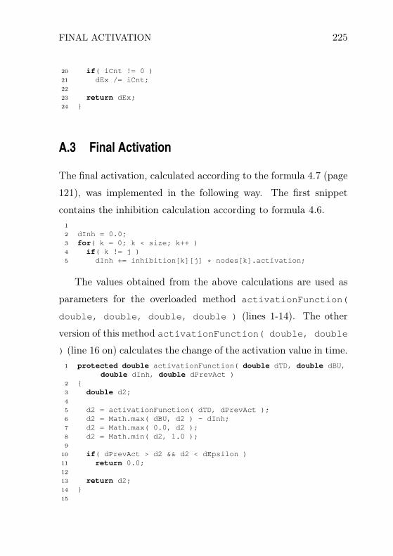
FINAL ACTIVATION 225
20 if( iCnt != 0 )21 dEx /= iCnt;22
23 return dEx;24
A.3 Final Activation
The final activation, calculated according to the formula 4.7 (page
121), was implemented in the following way. The first snippet
contains the inhibition calculation according to formula 4.6.
1
2 dInh = 0.0;3 for( k = 0; k < size; k++ )4 if( k != j )5 dInh += inhibition[k][j] * nodes[k].activation;
The values obtained from the above calculations are used as
parameters for the overloaded method activationFunction(
double, double, double, double ) (lines 1-14). The other
version of this method activationFunction( double, double
) (line 16 on) calculates the change of the activation value in time.
1 protected double activationFunction( double dTD, double dBU,double dInh, double dPrevAct )
2 3 double d2;4
5 d2 = activationFunction( dTD, dPrevAct );6 d2 = Math.max( dBU, d2 ) - dInh;7 d2 = Math.max( 0.0, d2 );8 d2 = Math.min( d2, 1.0 );9
10 if( dPrevAct > d2 && d2 < dEpsilon )11 return 0.0;12
13 return d2;14 15
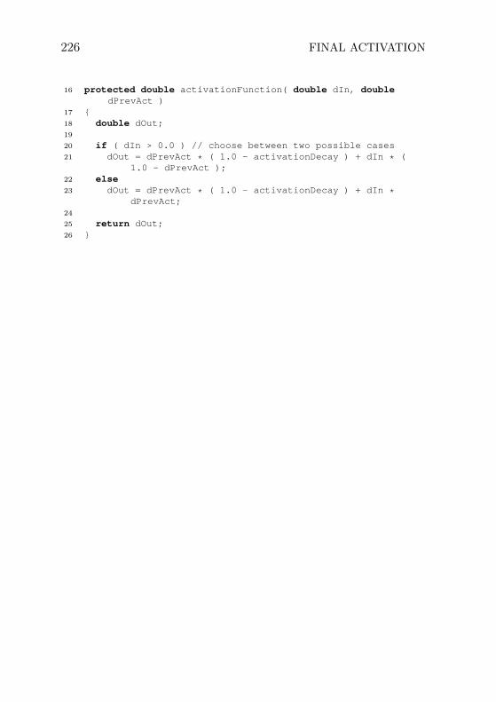
226 FINAL ACTIVATION
16 protected double activationFunction( double dIn, doubledPrevAct )
17 18 double dOut;19
20 if ( dIn > 0.0 ) // choose between two possible cases21 dOut = dPrevAct * ( 1.0 - activationDecay ) + dIn * (
1.0 - dPrevAct );22 else23 dOut = dPrevAct * ( 1.0 - activationDecay ) + dIn *
dPrevAct;24
25 return dOut;26
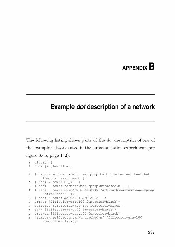
APPENDIX B
Example dot description of a network
The following listing shows parts of the dot description of one of
the example networks used in the autoassociation experiment (see
figure 6.6b, page 152).
1 digraph 2 node [style=filled]3
4 rank = source; armour selfprop tank tracked antitank hottow howitzer towed ;
5 rank = same; FH_70 ;6 rank = same; "armour\nselfprop\ntracked\n" ;7 rank = same; LEOPARD_2 PzH2000 "antitank\narmour\nselfprop
\ntracked\n" ;8 rank = same; JAGUAR_1 JAGUAR_2 ;9 armour [fillcolor=gray100 fontcolor=black];
10 selfprop [fillcolor=gray100 fontcolor=black];11 tank [fillcolor=gray100 fontcolor=black];12 tracked [fillcolor=gray100 fontcolor=black];13 "armour\nselfprop\ntank\ntracked\n" [fillcolor=gray100
fontcolor=black];
227

228
14 LEOPARD_2 [fillcolor=gray100 fontcolor=black];15 antitank [fillcolor=gray100 fontcolor=black];16 hot [fillcolor=gray100 fontcolor=black];17 "antitank\narmour\nhot\nselfprop\ntracked\n" [fillcolor=
gray100 fontcolor=black];18 JAGUAR_1 [fillcolor=gray100 fontcolor=black];19 tow [fillcolor=gray100 fontcolor=black];20 "antitank\narmour\nselfprop\ntow\ntracked\n" [fillcolor=
gray100 fontcolor=black];21 JAGUAR_2 [fillcolor=gray100 fontcolor=black];22 howitzer [fillcolor=gray100 fontcolor=black];23 towed [fillcolor=gray100 fontcolor=black];24 "howitzer\ntowed\n" [fillcolor=gray100 fontcolor=black];25 FH_70 [fillcolor=gray100 fontcolor=black];26 "armour\nhowitzer\nselfprop\ntracked\n" [fillcolor=gray100
fontcolor=black];27 PzH2000 [fillcolor=gray100 fontcolor=black];28 "armour\nselfprop\ntracked\n" [fillcolor=gray100 fontcolor=
black];29 "antitank\narmour\nselfprop\ntracked\n" [fillcolor=gray100
fontcolor=black];30 edge [color=black] armour -> "armour\nselfprop\ntracked\n";31 edge [color=black] selfprop -> "armour\nselfprop\ntracked\n"
;32 edge [color=black] tank -> "armour\nselfprop\ntank\ntracked\
n";33 "armour\nselfprop\ntank\ntracked\n" -> LEOPARD_2;34 edge [color=black] tracked -> "armour\nselfprop\ntracked\n";35 edge [color=black] antitank -> "antitank\narmour\nselfprop\
ntracked\n";36 edge [color=black] hot -> "antitank\narmour\nhot\nselfprop\
ntracked\n";37 "antitank\narmour\nhot\nselfprop\ntracked\n" -> JAGUAR_1;38 edge [color=black] tow -> "antitank\narmour\nselfprop\ntow\
ntracked\n";39 "antitank\narmour\nselfprop\ntow\ntracked\n" -> JAGUAR_2;40 edge [color=black] howitzer -> "howitzer\ntowed\n";41 "howitzer\ntowed\n" -> FH_70;42 edge [color=black] howitzer -> "armour\nhowitzer\nselfprop\
ntracked\n";43 "armour\nhowitzer\nselfprop\ntracked\n" -> PzH2000;44 edge [color=black] towed -> "howitzer\ntowed\n";45 edge [color=black] "armour\nselfprop\ntracked\n" -> "armour\
nselfprop\ntank\ntracked\n";46 edge [color=black] "armour\nselfprop\ntracked\n" -> "armour\
nhowitzer\nselfprop\ntracked\n";47 edge [color=black] "armour\nselfprop\ntracked\n" -> "
antitank\narmour\nselfprop\ntracked\n";

229
48 edge [color=black] "antitank\narmour\nselfprop\ntracked\n"-> "antitank\narmour\nhot\nselfprop\ntracked\n";
49 edge [color=black] "antitank\narmour\nselfprop\ntracked\n"-> "antitank\narmour\nselfprop\ntow\ntracked\n";
50