Embed Size (px)
Citation preview
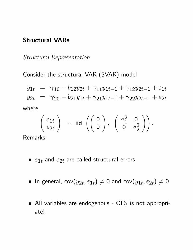
Structural VARs
Structural Representation
Consider the structural VAR (SVAR) model
y1t = γ10 − b12y2t + γ11y1t−1 + γ12y2t−1 + ε1t
y2t = γ20 − b21y1t + γ21y1t−1 + γ22y2t−1 + ε2t
where Ãε1tε2t
!∼ iid
ÃÃ00
!,
Ãσ21 00 σ22
!!.
Remarks:
• ε1t and ε2t are called structural errors
• In general, cov(y2t, ε1t) 6= 0 and cov(y1t, ε2t) 6= 0
• All variables are endogenous - OLS is not appropri-ate!
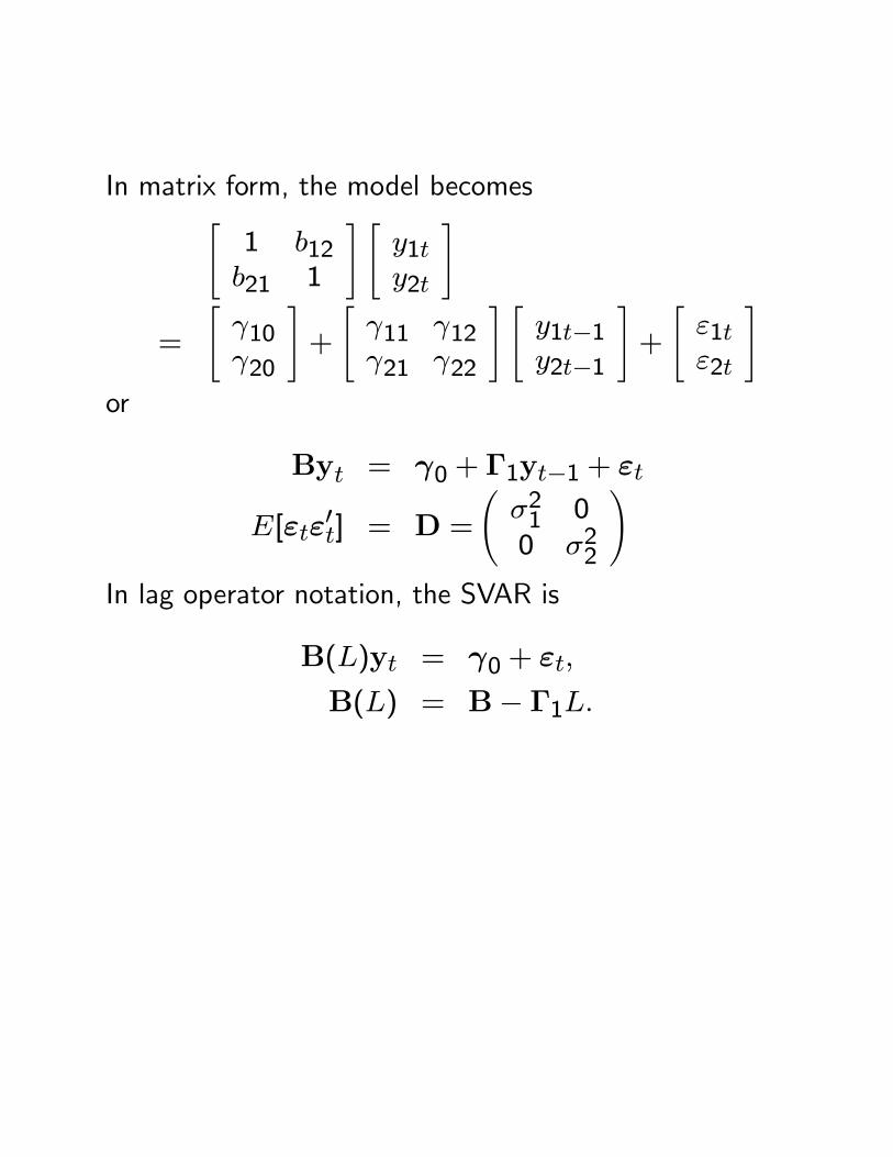
In matrix form, the model becomes"1 b12b21 1
# "y1ty2t
#
=
"γ10γ20
#+
"γ11 γ12γ21 γ22
# "y1t−1y2t−1
#+
"ε1tε2t
#or
Byt = γ0 + Γ1yt−1 + εt
E[εtε0t] = D =
Ãσ21 00 σ22
!In lag operator notation, the SVAR is
B(L)yt = γ0 + εt,
B(L) = B− Γ1L.
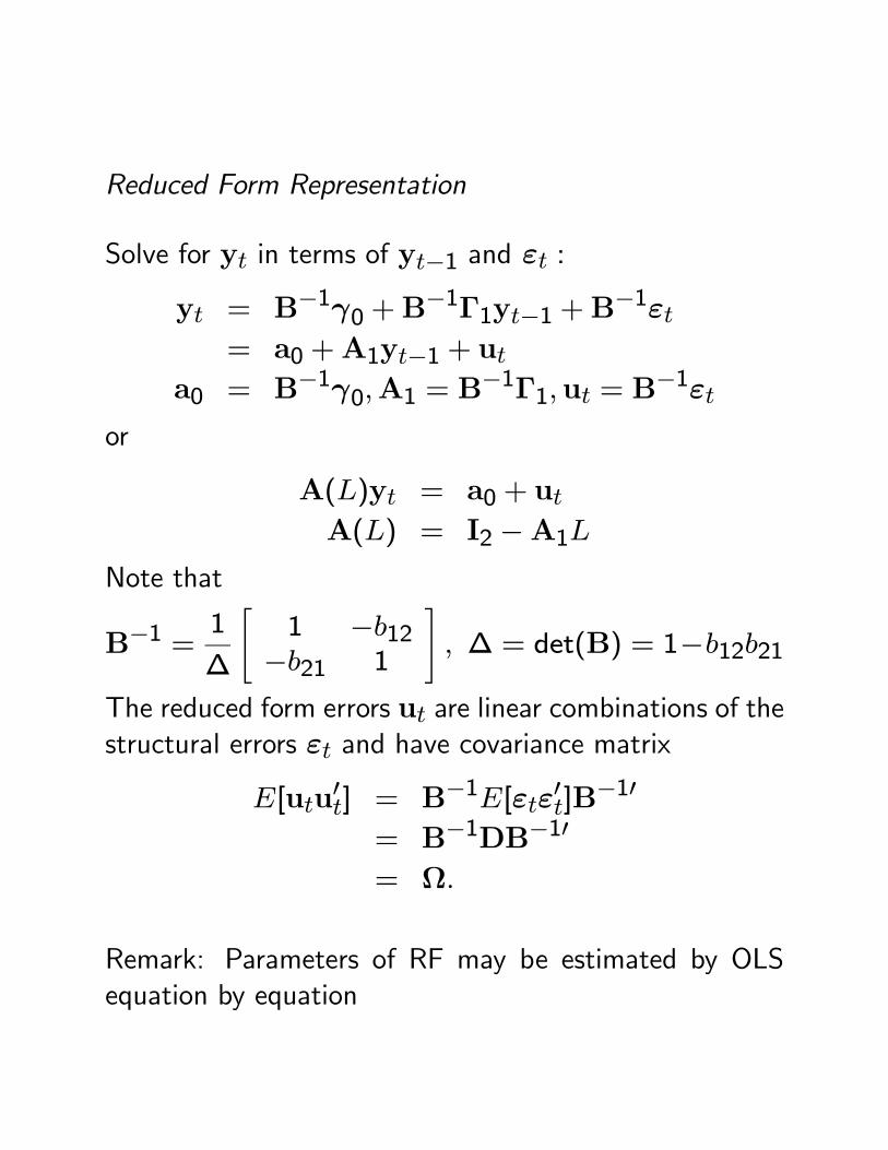
Reduced Form Representation
Solve for yt in terms of yt−1 and εt :
yt = B−1γ0 +B−1Γ1yt−1 +B
−1εt= a0 +A1yt−1 + ut
a0 = B−1γ0,A1 = B−1Γ1,ut = B
−1εtor
A(L)yt = a0 + utA(L) = I2 −A1L
Note that
B−1 =1
∆
"1 −b12−b21 1
#, ∆ = det(B) = 1−b12b21
The reduced form errors ut are linear combinations of thestructural errors εt and have covariance matrix
E[utu0t] = B−1E[εtε0t]B
−10
= B−1DB−10
= Ω.
Remark: Parameters of RF may be estimated by OLSequation by equation
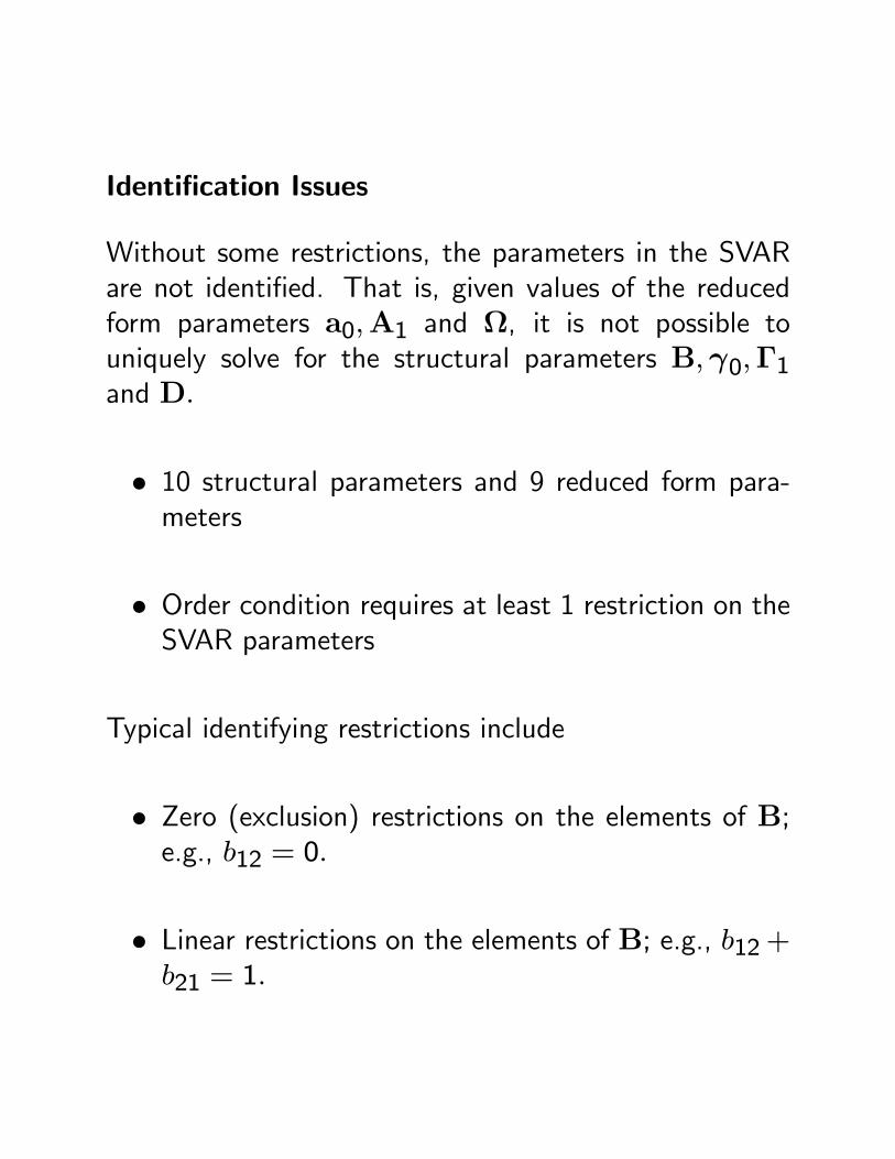
Identification Issues
Without some restrictions, the parameters in the SVARare not identified. That is, given values of the reducedform parameters a0,A1 and Ω, it is not possible touniquely solve for the structural parameters B,γ0,Γ1and D.
• 10 structural parameters and 9 reduced form para-meters
• Order condition requires at least 1 restriction on theSVAR parameters
Typical identifying restrictions include
• Zero (exclusion) restrictions on the elements of B;e.g., b12 = 0.
• Linear restrictions on the elements of B; e.g., b12 +b21 = 1.
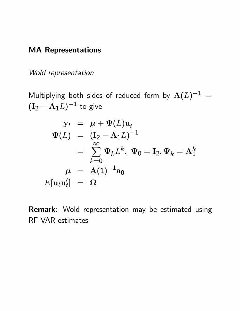
MA Representations
Wold representation
Multiplying both sides of reduced form by A(L)−1 =(I2 −A1L)−1 to give
yt = μ+Ψ(L)utΨ(L) = (I2 −A1L)−1
=∞Xk=0
ΨkLk, Ψ0 = I2,Ψk = A
k1
μ = A(1)−1a0E[utu
0t] = Ω
Remark: Wold representation may be estimated usingRF VAR estimates
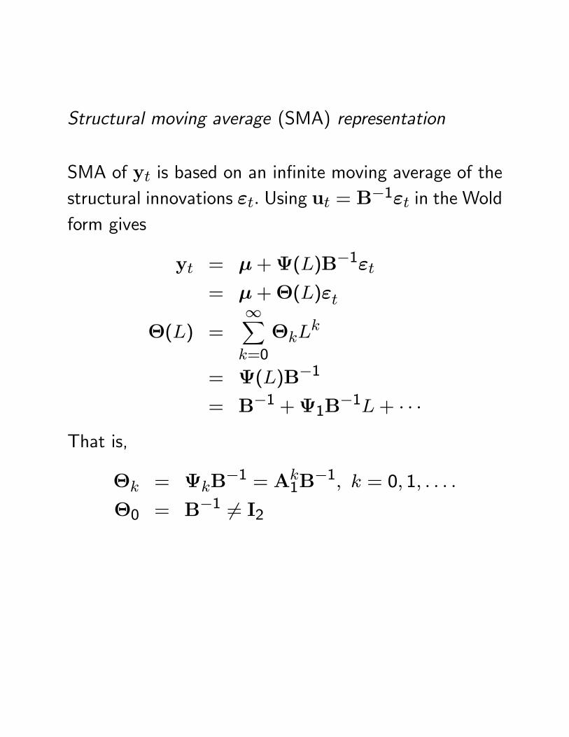
Structural moving average (SMA) representation
SMA of yt is based on an infinite moving average of thestructural innovations εt. Using ut = B−1εt in the Woldform gives
yt = μ+Ψ(L)B−1εt= μ+Θ(L)εt
Θ(L) =∞Xk=0
ΘkLk
= Ψ(L)B−1
= B−1 +Ψ1B−1L+ · · ·
That is,
Θk = ΨkB−1 = Ak
1B−1, k = 0, 1, . . . .
Θ0 = B−1 6= I2
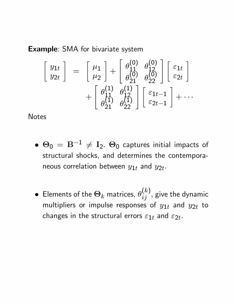
Example: SMA for bivariate system"y1ty2t
#=
"μ1μ2
#+
⎡⎣ θ(0)11 θ
(0)12
θ(0)21 θ
(0)22
⎤⎦ " ε1tε2t
#
+
⎡⎣ θ(1)11 θ
(1)12
θ(1)21 θ
(1)22
⎤⎦ " ε1t−1ε2t−1
#+ · · ·
Notes
• Θ0 = B−1 6= I2. Θ0 captures initial impacts ofstructural shocks, and determines the contempora-neous correlation between y1t and y2t.
• Elements of theΘk matrices, θ(k)ij , give the dynamic
multipliers or impulse responses of y1t and y2t tochanges in the structural errors ε1t and ε2t.
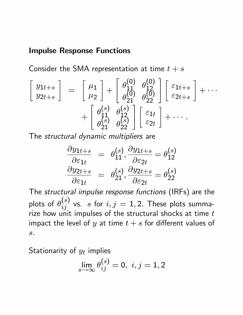
Impulse Response Functions
Consider the SMA representation at time t+ s"y1t+sy2t+s
#=
"μ1μ2
#+
⎡⎣ θ(0)11 θ
(0)12
θ(0)21 θ
(0)22
⎤⎦ " ε1t+sε2t+s
#+ · · ·
+
⎡⎣ θ(s)11 θ
(s)12
θ(s)21 θ
(s)22
⎤⎦ " ε1tε2t
#+ · · · .
The structural dynamic multipliers are
∂y1t+s∂ε1t
= θ(s)11 ,
∂y1t+s∂ε2t
= θ(s)12
∂y2t+s∂ε1t
= θ(s)21 ,
∂y2t+s∂ε2t
= θ(s)22
The structural impulse response functions (IRFs) are the
plots of θ(s)ij vs. s for i, j = 1, 2. These plots summa-rize how unit impulses of the structural shocks at time timpact the level of y at time t+ s for different values ofs.
Stationarity of yt implies
lims→∞ θ
(s)ij = 0, i, j = 1, 2
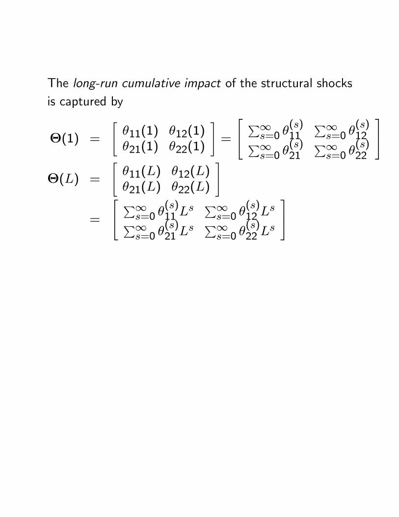
The long-run cumulative impact of the structural shocksis captured by
Θ(1) =
"θ11(1) θ12(1)θ21(1) θ22(1)
#=
⎡⎣ P∞s=0 θ(s)11 P∞s=0 θ
(s)12P∞
s=0 θ(s)21
P∞s=0 θ
(s)22
⎤⎦Θ(L) =
"θ11(L) θ12(L)θ21(L) θ22(L)
#
=
⎡⎣ P∞s=0 θ(s)11 Ls P∞s=0 θ
(s)12 L
sP∞s=0 θ
(s)21 L
s P∞s=0 θ
(s)22 L
s
⎤⎦
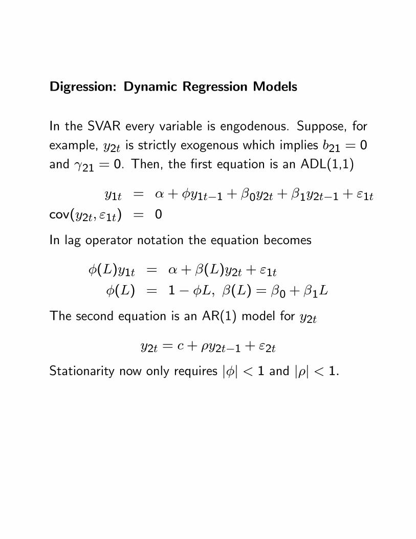
Digression: Dynamic Regression Models
In the SVAR every variable is engodenous. Suppose, forexample, y2t is strictly exogenous which implies b21 = 0and γ21 = 0. Then, the first equation is an ADL(1,1)
y1t = α+ φy1t−1 + β0y2t + β1y2t−1 + ε1t
cov(y2t, ε1t) = 0
In lag operator notation the equation becomes
φ(L)y1t = α+ β(L)y2t + ε1t
φ(L) = 1− φL, β(L) = β0 + β1L
The second equation is an AR(1) model for y2t
y2t = c+ ρy2t−1 + ε2t
Stationarity now only requires |φ| < 1 and |ρ| < 1.
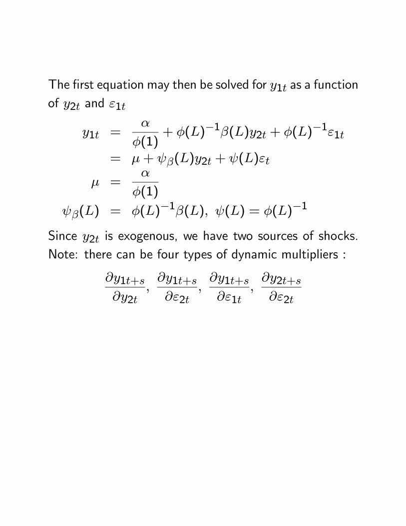
The first equation may then be solved for y1t as a functionof y2t and ε1t
y1t =α
φ(1)+ φ(L)−1β(L)y2t + φ(L)−1ε1t
= μ+ ψβ(L)y2t + ψ(L)εt
μ =α
φ(1)
ψβ(L) = φ(L)−1β(L), ψ(L) = φ(L)−1
Since y2t is exogenous, we have two sources of shocks.Note: there can be four types of dynamic multipliers :
∂y1t+s∂y2t
,∂y1t+s∂ε2t
,∂y1t+s∂ε1t
,∂y2t+s∂ε2t
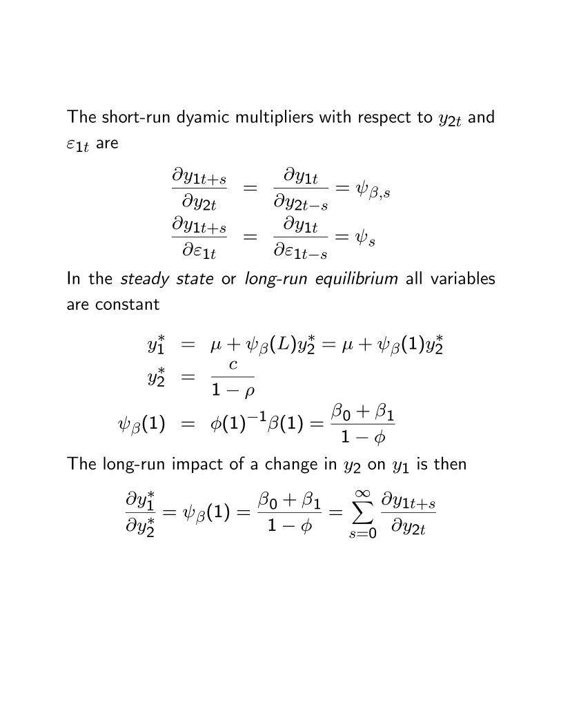
The short-run dyamic multipliers with respect to y2t andε1t are
∂y1t+s∂y2t
=∂y1t∂y2t−s
= ψβ,s
∂y1t+s∂ε1t
=∂y1t∂ε1t−s
= ψs
In the steady state or long-run equilibrium all variablesare constant
y∗1 = μ+ ψβ(L)y∗2 = μ+ ψβ(1)y
∗2
y∗2 =c
1− ρ
ψβ(1) = φ(1)−1β(1) =β0 + β11− φ
The long-run impact of a change in y2 on y1 is then
∂y∗1∂y∗2
= ψβ(1) =β0 + β11− φ
=∞Xs=0
∂y1t+s∂y2t
Identification issues
In some applications, identification of the parameters ofthe SVAR is achieved through restrictions on the para-meters of the SMA representation.
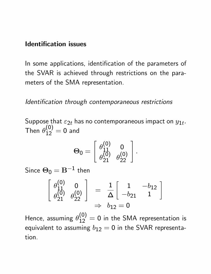
Identification through contemporaneous restrictions
Suppose that ε2t has no contemporaneous impact on y1t.Then θ(0)12 = 0 and
Θ0 =
⎡⎣ θ(0)11 0
θ(0)21 θ
(0)22
⎤⎦ .Since Θ0 = B−1 then⎡⎣ θ
(0)11 0
θ(0)21 θ
(0)22
⎤⎦ =1
∆
"1 −b12−b21 1
#⇒ b12 = 0
Hence, assuming θ(0)12 = 0 in the SMA representation isequivalent to assuming b12 = 0 in the SVAR representa-tion.
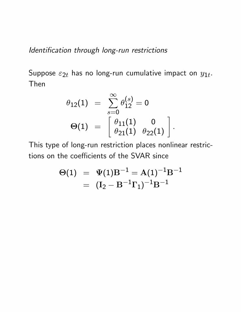
Identification through long-run restrictions
Suppose ε2t has no long-run cumulative impact on y1t.Then
θ12(1) =∞Xs=0
θ(s)12 = 0
Θ(1) =
"θ11(1) 0θ21(1) θ22(1)
#.
This type of long-run restriction places nonlinear restric-tions on the coefficients of the SVAR since
Θ(1) = Ψ(1)B−1 = A(1)−1B−1
= (I2 −B−1Γ1)−1B−1
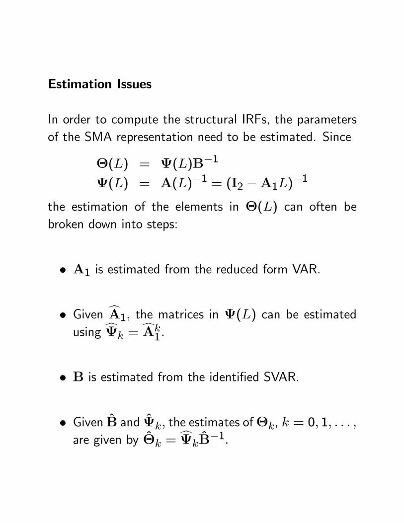
Estimation Issues
In order to compute the structural IRFs, the parametersof the SMA representation need to be estimated. Since
Θ(L) = Ψ(L)B−1
Ψ(L) = A(L)−1 = (I2 −A1L)−1
the estimation of the elements in Θ(L) can often bebroken down into steps:
• A1 is estimated from the reduced form VAR.
• Given cA1, the matrices in Ψ(L) can be estimatedusing cΨk =
cAk1.
• B is estimated from the identified SVAR.
• Given B and Ψk, the estimates ofΘk, k = 0, 1, . . . ,are given by Θk =
cΨkB−1.
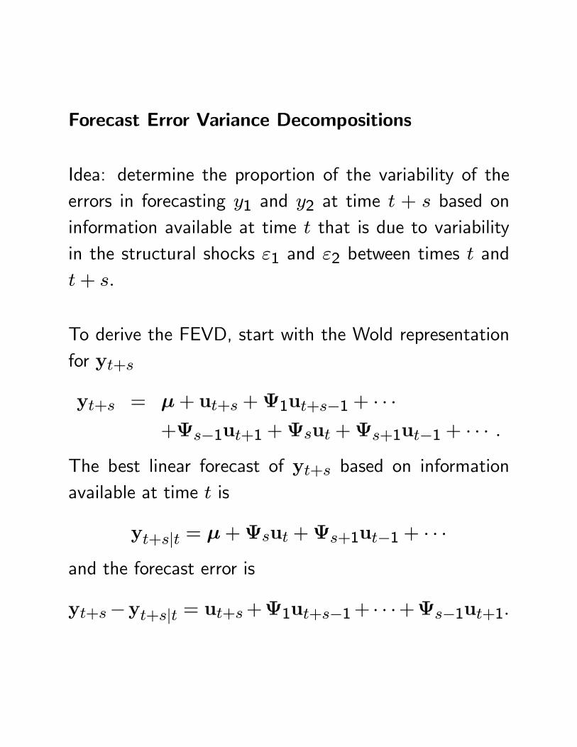
Forecast Error Variance Decompositions
Idea: determine the proportion of the variability of theerrors in forecasting y1 and y2 at time t + s based oninformation available at time t that is due to variabilityin the structural shocks ε1 and ε2 between times t andt+ s.
To derive the FEVD, start with the Wold representationfor yt+s
yt+s = μ+ ut+s +Ψ1ut+s−1 + · · ·+Ψs−1ut+1 +Ψsut +Ψs+1ut−1 + · · · .
The best linear forecast of yt+s based on informationavailable at time t is
yt+s|t = μ+Ψsut +Ψs+1ut−1 + · · ·
and the forecast error is
yt+s−yt+s|t = ut+s+Ψ1ut+s−1+ · · ·+Ψs−1ut+1.
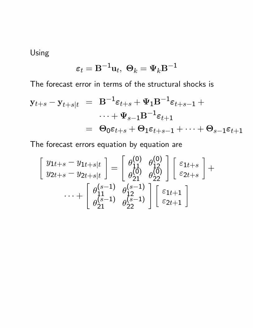
Using
εt = B−1ut, Θk = ΨkB
−1
The forecast error in terms of the structural shocks is
yt+s − yt+s|t = B−1εt+s +Ψ1B−1εt+s−1 +
· · ·+Ψs−1B−1εt+1
= Θ0εt+s +Θ1εt+s−1 + · · ·+Θs−1εt+1
The forecast errors equation by equation are"y1t+s − y1t+s|ty2t+s − y2t+s|t
#=
⎡⎣ θ(0)11 θ
(0)12
θ(0)21 θ
(0)22
⎤⎦ " ε1t+sε2t+s
#+
· · ·+⎡⎣ θ
(s−1)11 θ
(s−1)12
θ(s−1)21 θ
(s−1)22
⎤⎦ " ε1t+1ε2t+1
#
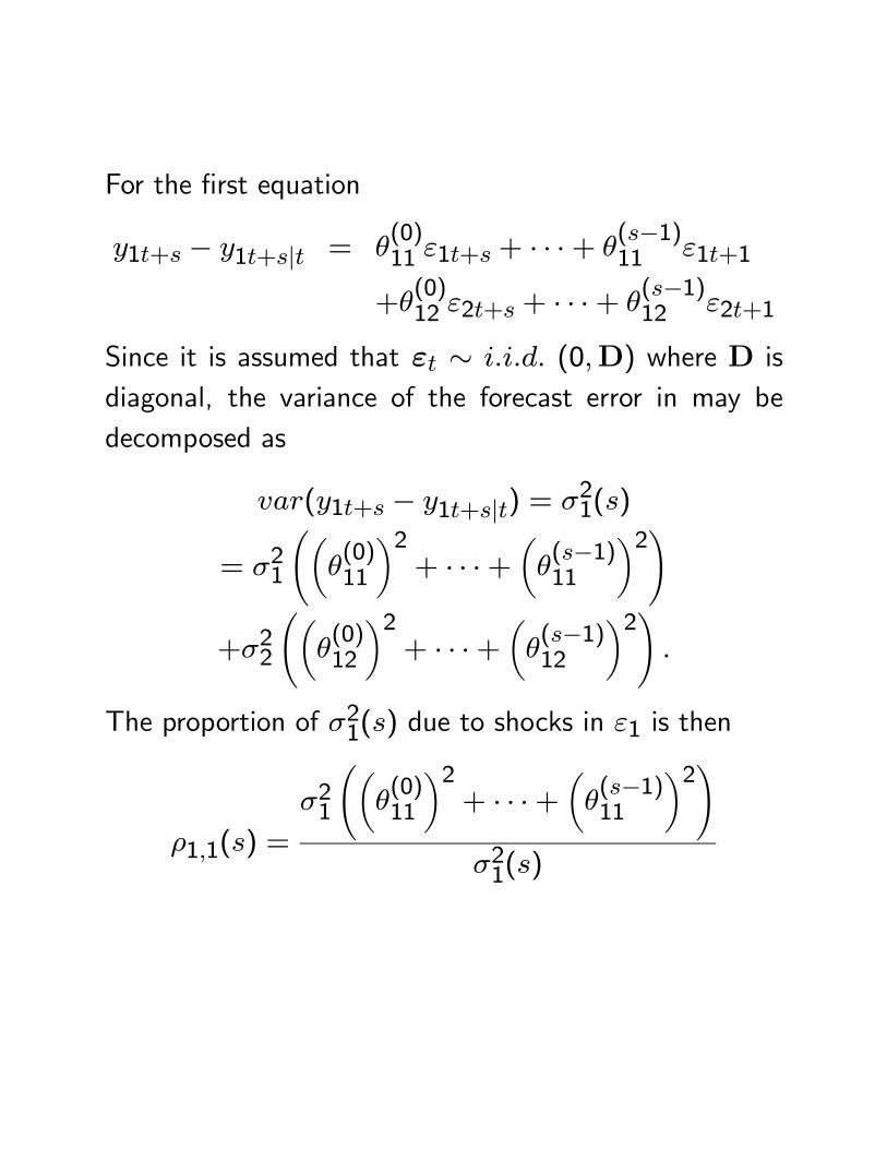
For the first equation
y1t+s − y1t+s|t = θ(0)11 ε1t+s + · · ·+ θ
(s−1)11 ε1t+1
+θ(0)12 ε2t+s + · · ·+ θ
(s−1)12 ε2t+1
Since it is assumed that εt ∼ i.i.d. (0,D) where D isdiagonal, the variance of the forecast error in may bedecomposed as
var(y1t+s − y1t+s|t) = σ21(s)
= σ21
õθ(0)11
¶2+ · · ·+
µθ(s−1)11
¶2!
+σ22
õθ(0)12
¶2+ · · ·+
µθ(s−1)12
¶2!.
The proportion of σ21(s) due to shocks in ε1 is then
ρ1,1(s) =
σ21
õθ(0)11
¶2+ · · ·+
µθ(s−1)11
¶2!σ21(s)
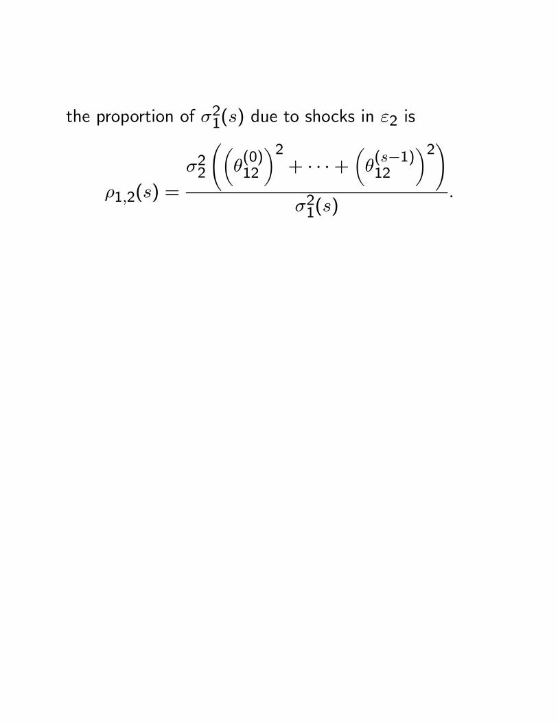
the proportion of σ21(s) due to shocks in ε2 is
ρ1,2(s) =
σ22
õθ(0)12
¶2+ · · ·+
µθ(s−1)12
¶2!σ21(s)
.
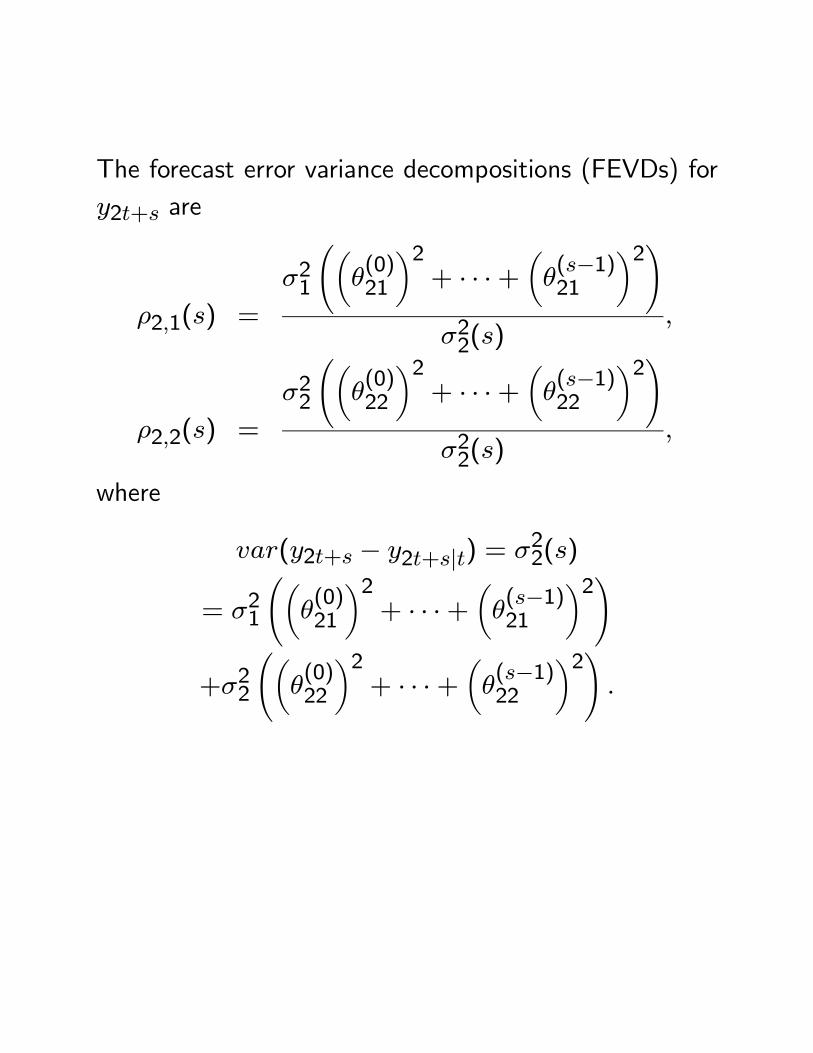
The forecast error variance decompositions (FEVDs) fory2t+s are
ρ2,1(s) =
σ21
õθ(0)21
¶2+ · · ·+
µθ(s−1)21
¶2!σ22(s)
,
ρ2,2(s) =
σ22
õθ(0)22
¶2+ · · ·+
µθ(s−1)22
¶2!σ22(s)
,
where
var(y2t+s − y2t+s|t) = σ22(s)
= σ21
õθ(0)21
¶2+ · · ·+
µθ(s−1)21
¶2!
+σ22
õθ(0)22
¶2+ · · ·+
µθ(s−1)22
¶2!.
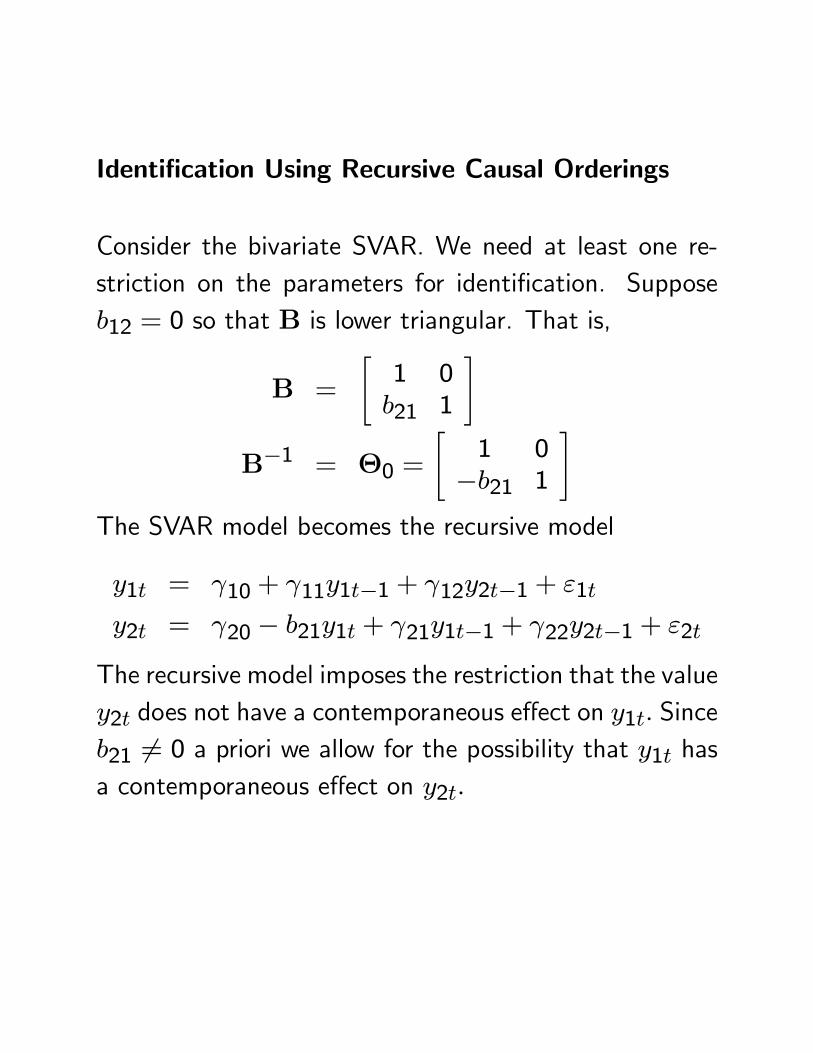
Identification Using Recursive Causal Orderings
Consider the bivariate SVAR. We need at least one re-striction on the parameters for identification. Supposeb12 = 0 so that B is lower triangular. That is,
B =
"1 0b21 1
#
B−1 = Θ0 =
"1 0−b21 1
#The SVAR model becomes the recursive model
y1t = γ10 + γ11y1t−1 + γ12y2t−1 + ε1t
y2t = γ20 − b21y1t + γ21y1t−1 + γ22y2t−1 + ε2t
The recursive model imposes the restriction that the valuey2t does not have a contemporaneous effect on y1t. Sinceb21 6= 0 a priori we allow for the possibility that y1t hasa contemporaneous effect on y2t.
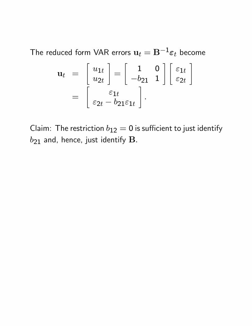
The reduced form VAR errors ut = B−1εt become
ut =
"u1tu2t
#=
"1 0−b21 1
# "ε1tε2t
#
=
"ε1t
ε2t − b21ε1t
#.
Claim: The restriction b12 = 0 is sufficient to just identifyb21 and, hence, just identify B.
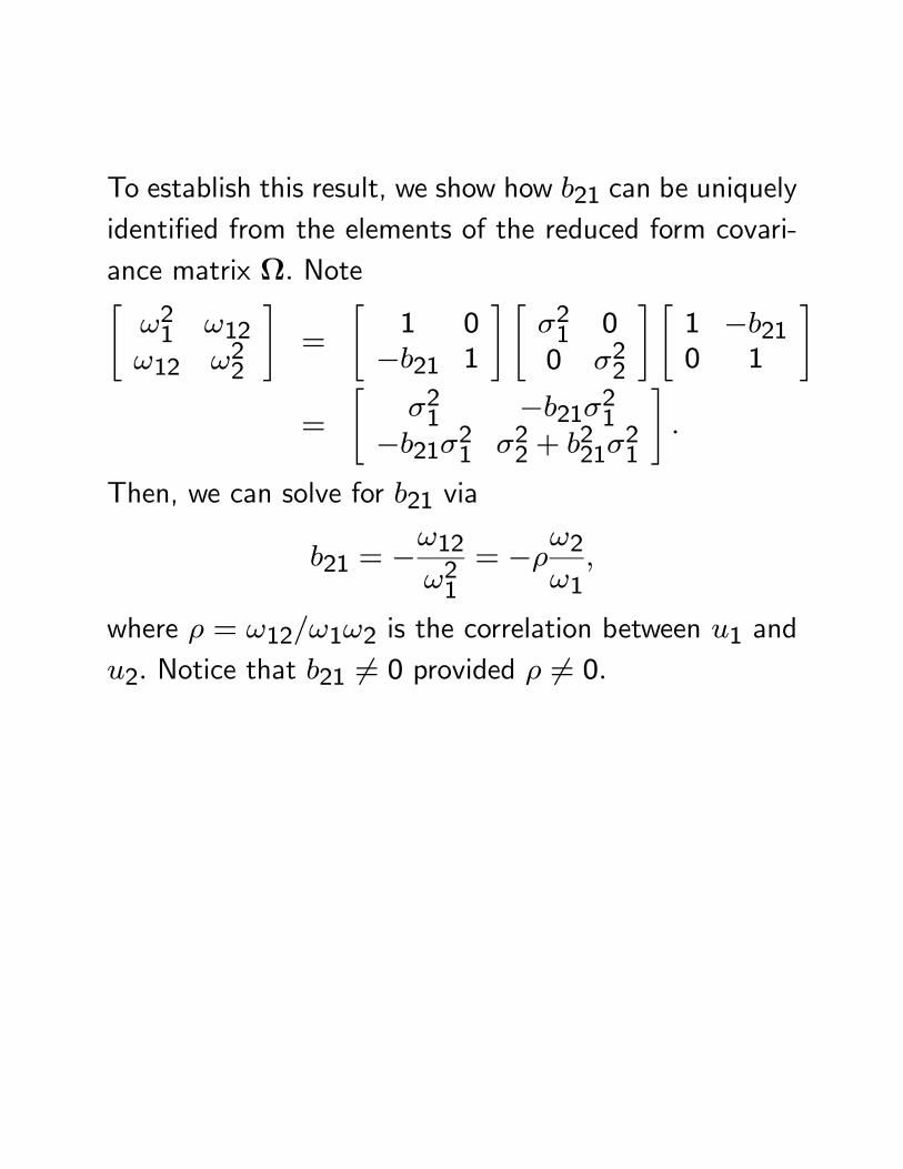
To establish this result, we show how b21 can be uniquelyidentified from the elements of the reduced form covari-ance matrix Ω. Note"ω21 ω12ω12 ω22
#=
"1 0−b21 1
# "σ21 00 σ22
# "1 −b210 1
#
=
"σ21 −b21σ21
−b21σ21 σ22 + b221σ21
#.
Then, we can solve for b21 via
b21 = −ω12ω21
= −ρω2ω1
,
where ρ = ω12/ω1ω2 is the correlation between u1 andu2. Notice that b21 6= 0 provided ρ 6= 0.
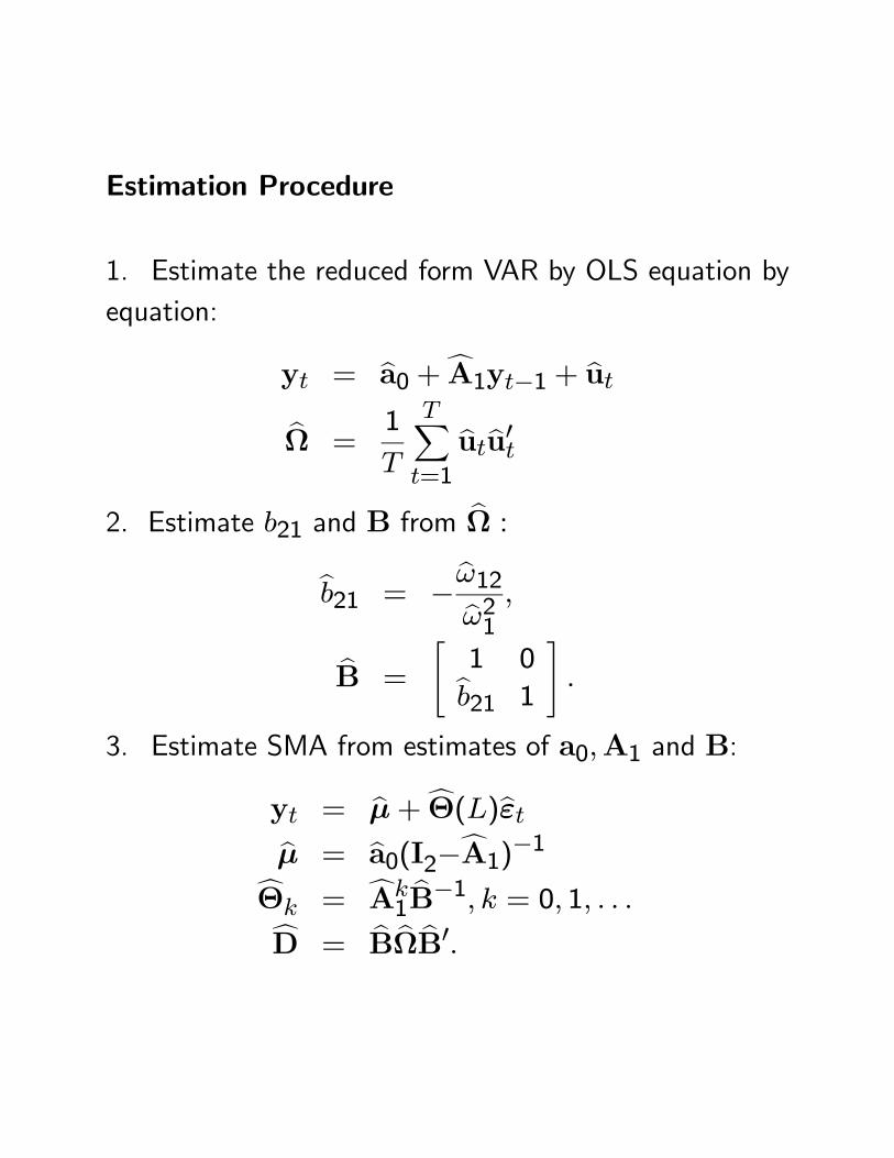
Estimation Procedure
1. Estimate the reduced form VAR by OLS equation byequation:
yt = ba0 +cA1yt−1 + butbΩ =
1
T
TXt=1
butbu0t2. Estimate b21 and B from bΩ :
bb21 = −bω12bω21 ,bB =
"1 0bb21 1
#.
3. Estimate SMA from estimates of a0,A1 and B:
yt = bμ+cΘ(L)bεtbμ = ba0(I2−cA1)−1cΘk = cAk1bB−1, k = 0, 1, . . .cD = bB bΩ bB0.
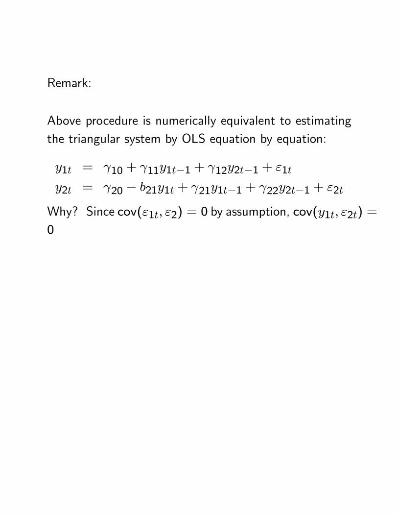
Remark:
Above procedure is numerically equivalent to estimatingthe triangular system by OLS equation by equation:
y1t = γ10 + γ11y1t−1 + γ12y2t−1 + ε1t
y2t = γ20 − b21y1t + γ21y1t−1 + γ22y2t−1 + ε2t
Why? Since cov(ε1t, ε2) = 0 by assumption, cov(y1t, ε2t) =0
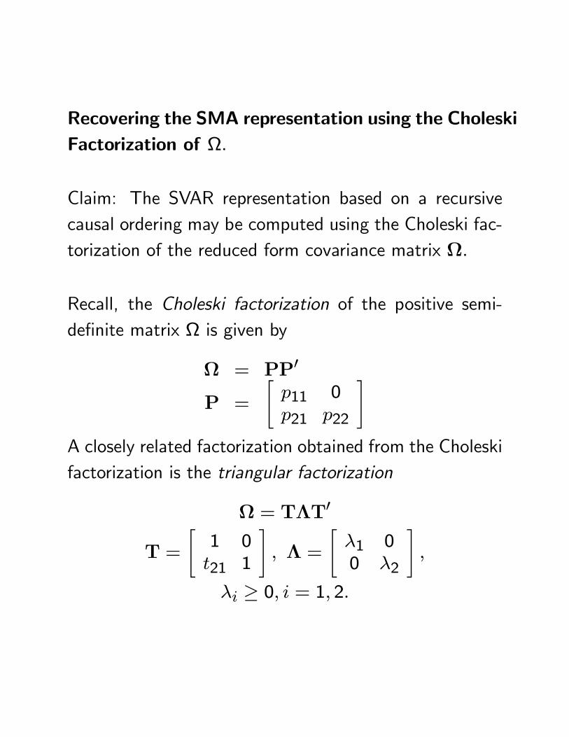
Recovering the SMA representation using the CholeskiFactorization of Ω.
Claim: The SVAR representation based on a recursivecausal ordering may be computed using the Choleski fac-torization of the reduced form covariance matrix Ω.
Recall, the Choleski factorization of the positive semi-definite matrix Ω is given by
Ω = PP0
P =
"p11 0p21 p22
#A closely related factorization obtained from the Choleskifactorization is the triangular factorization
Ω = TΛT0
T =
"1 0t21 1
#, Λ =
"λ1 00 λ2
#,
λi ≥ 0, i = 1, 2.
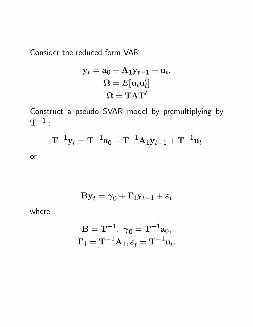
Consider the reduced form VAR
yt = a0 +A1yt−1 + ut,
Ω = E[utu0t]
Ω = TΛT0
Construct a pseudo SVAR model by premultiplying byT−1 :
T−1yt = T−1a0 +T−1A1yt−1 +T
−1ut
or
Byt = γ0 + Γ1yt−1 + εt
where
B = T−1, γ0 = T−1a0,
Γ1 = T−1A1, εt = T
−1ut.
The pseudo structural errors εt have a diagonal covari-ance matrix Λ
E[εtε0t] = T−1E[utu0t]T
−10
= T−1ΩT−10
= T−1TΛT0T−10
= Λ.
In the pseudo SVAR,
B =
"1 0b21 1
#= T−1 =
"1 0−t21 1
#b12 = 0, b21 = −t21
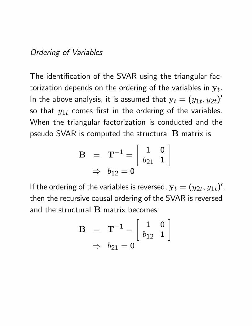
Ordering of Variables
The identification of the SVAR using the triangular fac-torization depends on the ordering of the variables in yt.In the above analysis, it is assumed that yt = (y1t, y2t)0
so that y1t comes first in the ordering of the variables.When the triangular factorization is conducted and thepseudo SVAR is computed the structural B matrix is
B = T−1 =
"1 0b21 1
#⇒ b12 = 0
If the ordering of the variables is reversed, yt = (y2t, y1t)0,then the recursive causal ordering of the SVAR is reversedand the structural B matrix becomes
B = T−1 =
"1 0b12 1
#⇒ b21 = 0
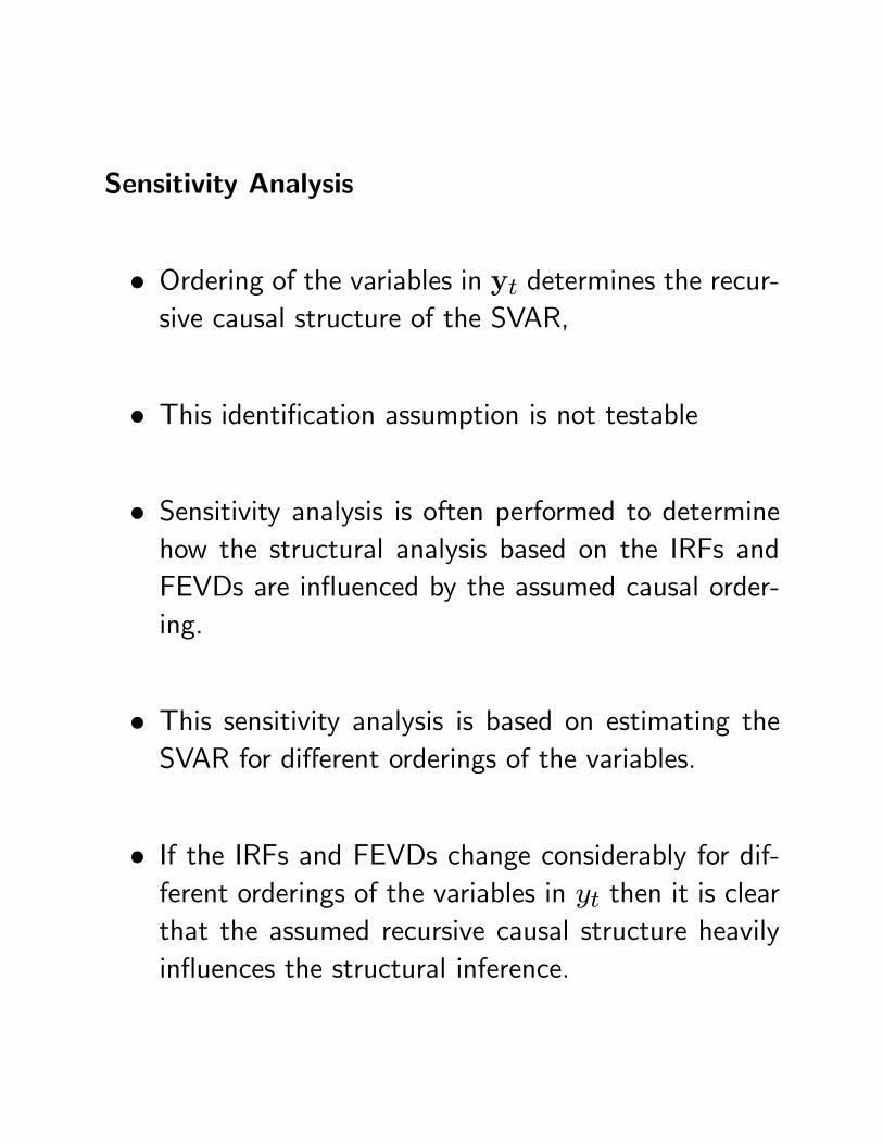
Sensitivity Analysis
• Ordering of the variables in yt determines the recur-sive causal structure of the SVAR,
• This identification assumption is not testable
• Sensitivity analysis is often performed to determinehow the structural analysis based on the IRFs andFEVDs are influenced by the assumed causal order-ing.
• This sensitivity analysis is based on estimating theSVAR for different orderings of the variables.
• If the IRFs and FEVDs change considerably for dif-ferent orderings of the variables in yt then it is clearthat the assumed recursive causal structure heavilyinfluences the structural inference.
Residual Analysis
One way to determine if the assumed causal ordering in-fluences the structural inferences is to look at the resid-ual covariance matrix Ω from the estimated reduced formVAR. If this covariance matrix is close to being diagonalthen the estimated value of B will be close to diagonaland so the ordering of the variables will not influence thestructural inference.