Constructive Algebra in Functional Programming and Type Theory

Master of Science Thesis in the Programme Computer Science – Algorithms, Languages and Logic

���������AB��C

DEF��������������������A��E��������������������C��E��� ����!F����������D��! ������������F�"������������C#������$��%�"��$���F��&'('

AE��� �E�����F�������DEF��������������������A��E�������F�"���������������C��E��� ����E�����)�*�� ��������E�����! ����E��E��+��,�����������F����F�"����F����)��������F��! �!�����F,�����F��������������E��-�������.�AE��� �E���%F��F�����EF��E�/�E������E��F �E�������E��+��,$�F�"�%F��F�����EF���E��+��,�"������������F�����*�$�!��� ���������E����F����F���EF������F������!����E���F%.�

AE��� �E����EF��$�%E�����F�����������E�����E�������E��+��,����F��E��"�!F����0�����*F�!���F�! ����E������F����!F��1$�F�,��%��"����E���E��"�!F����F�� ���E���F��������.�-���E��� �E���EF�������"�F���!����E��F���������%��E�F��E��"�!F�������F�"�����E��+��,$��E��� �E���%F��F����E�������EF��E�/�E��EF�����F���"�F���������F���!����������������E����E��"�!F�����������DEF��������������������A��E�������F�"���������������C��E��� �����������E��+��,�����������F����F�"��F,�����F��������������E��-�������.

Constructive Algebra in Functional Programming and Type Theory

Anders Mörtberg

© Anders Mörtberg, May 2010

Examiner: Prof. Thierry Coquand

Chalmers University of TechnologyUniversity of GothenburgDepartment of Computer Science and EngineeringSE-412 96 GöteborgSwedenTelephone + 46 (0)31-772 1000

Cover:An exact sequence defining that the module M is finitely presented. This is related to the notion of coherent rings presented in chapter 3.

Department of Computer Science and EngineeringC#������$��%�"����F��&'('

Abstract

This thesis considers abstract algebra from a constructive point of view. Thecentral concept of study is coherent rings − algebraic structures in which it ispossible to solve homogeneous systems of linear equations. Three different alge-braic theories are considered; Bézout domains, Prüfer domains and polynomialrings. The first two of these are non-Noetherian analogues of classical notions.The polynomial rings are presented from a constructive point of view with atreatment of Gröbner bases. The goal of the thesis is to study the proofs thatthese theories are coherent and explore how the proofs can be implemented infunctional programming and type theory.

Acknowledgments

First of all I would like to thank Thierry Coquand for all help and supportduring the work on this thesis.

I would also like to thank Bassel Mannaa for interesting discussions and helpwith the implementation. The comments presented during the opposition wasalso very helpful.

Finally I would like to thank everyone that has read and given constructiveand helpful comments on this thesis.

Contents

1 Introduction 1

1.1 Background . . . . . . . . . . . . . . . . . . . . . . . . . . . . . . 11.2 Method . . . . . . . . . . . . . . . . . . . . . . . . . . . . . . . . 21.3 Previous work . . . . . . . . . . . . . . . . . . . . . . . . . . . . . 21.4 Outline . . . . . . . . . . . . . . . . . . . . . . . . . . . . . . . . 3

2 Introduction to ring theory 5

2.1 Rings . . . . . . . . . . . . . . . . . . . . . . . . . . . . . . . . . 52.2 Ideals . . . . . . . . . . . . . . . . . . . . . . . . . . . . . . . . . 82.3 Discrete and strongly discrete rings . . . . . . . . . . . . . . . . . 102.4 Noetherian rings and Dedekind domains . . . . . . . . . . . . . . 10

3 Coherent rings 11

3.1 Definition and properties . . . . . . . . . . . . . . . . . . . . . . . 113.2 Coherence and strongly discrete rings . . . . . . . . . . . . . . . 14

4 Bézout domains 15

4.1 Definition . . . . . . . . . . . . . . . . . . . . . . . . . . . . . . . 154.2 Euclidean domains . . . . . . . . . . . . . . . . . . . . . . . . . . 164.3 Coherence of Bézout domains . . . . . . . . . . . . . . . . . . . . 174.4 Bézout domains and strong discreteness . . . . . . . . . . . . . . 184.5 GCD domains and fields of fractions . . . . . . . . . . . . . . . . 18

5 Prüfer domains 21

5.1 Definition . . . . . . . . . . . . . . . . . . . . . . . . . . . . . . . 215.2 Principal localization matrices . . . . . . . . . . . . . . . . . . . . 225.3 Invertible ideals and coherence of Prüfer domains . . . . . . . . . 255.4 Ideal arithmetic . . . . . . . . . . . . . . . . . . . . . . . . . . . . 275.5 Examples of Prüfer domains . . . . . . . . . . . . . . . . . . . . . 275.6 Prüfer domains and strong discreteness . . . . . . . . . . . . . . . 31

6 Polynomial rings 33

6.1 Monomials and monomial orderings . . . . . . . . . . . . . . . . 336.2 Polynomial rings . . . . . . . . . . . . . . . . . . . . . . . . . . . 346.3 Properties of ideals in k[x1, . . . , xn] . . . . . . . . . . . . . . . . . 366.4 Gröbner bases . . . . . . . . . . . . . . . . . . . . . . . . . . . . . 366.5 Coherence of k[x1, . . . , xn] . . . . . . . . . . . . . . . . . . . . . . 386.6 Strong discreteness of k[x1, . . . , xn] . . . . . . . . . . . . . . . . . 39

i

7 Conclusions 41

7.1 Implementation . . . . . . . . . . . . . . . . . . . . . . . . . . . . 417.2 Discussion . . . . . . . . . . . . . . . . . . . . . . . . . . . . . . . 457.3 Further work . . . . . . . . . . . . . . . . . . . . . . . . . . . . . 46

ii

Chapter 1

Introduction

1.1 Background

”It is important to keep in mind that constructive algebra isalgebra; in fact it is a generalization of algebra in that we do notassume the law of excluded middle.” [16]

Why is it that elementary algebra is so full of algorithms while advanced algebrais so full of nonconstructive arguments? Elementary algebra has factorizationof polynomials, equation solving and matrix inversion. Advanced algebra onthe other hand has notions such as arbitrary ideals of rings, prime and maximalideals and Noetherian assumptions on rings [4]. For example, both the existenceof maximal and prime ideals are usually proved using Zorn’s lemma. Zorn’slemma relies on the axiom of choice which in turn implies the law of excludedmiddle [19].

Modern abstract algebra begun with the introduction of algebraic struc-tures in the end of the 19th century. In the first half of the 20th centurynonconstructive methods dominated. In 1967 Erret Bishop published a bookcalled Foundations of Constructive Analysis which aimed to show that analysiscould be approached constructively. This, together with increasingly powerfulcomputers, led to a renaissance of constructive mathematics [16].

One of the main reasons to study constructive algebra is that it can give riseto new algorithms and ways to explore algebra using computers. The notion ofcomputation is at the core of constructive mathematics. A constructive proofof the existence of a mathematical object gives a way to construct the objectwhile a nonconstructive proof just proves the existence of such an object withoutnecessarily giving a way to construct it. For example, a constructive proof thata polynomial can be factorized as a product of irreducible polynomials mustprovide the factorization while a nonconstructive proof just have to prove theexistence of such a factorization without giving any witness of it.

Another reason to study constructive algebra is that it makes it possible torepresent advanced algebra in type theory and thus to verify the correctness ofmathematical proofs using computers. The reasons for this are the proofs-as-programs correspondence and the Brouwer-Heyting-Kolmogorov interpretationof intuitionistic logic which together give a way for representing mathematicalpropositions as types and proofs as programs. Note that it is also possible to ver-

1

ify classical mathematics using computers, but the point is that in constructivemathematics the proofs correspond to algorithms.

This thesis explores the question of how advanced algebra can be made con-structive by considering classical structures where the assumptions of Noethe-rianity has been dropped. This will be defined and discussed further in theintroduction to ring theory in chapter 2.

In linear algebra one of the main questions is how to solve homogeneoussystems of linear equations, but in linear algebra the central notion is vectorspaces which relies on the assumption that all nonzero elements has a multi-plicative inverse. One main aim of this thesis is to look at what happens if thisassumption is dropped. The proofs of the results should be constructive and beimplemented in a functional programming language and eventually also verifiedin a constructive proof system.

1.2 Method

The results presented in this thesis has been implemented in the pure lazy func-tional programming language Haskell. The reason for using Haskell is that it hasa powerful type system and the features that makes it suitable for implementingalgebraic theories are mainly polymorphism and the type class system.

In order to specify the axioms of algebraic structures the automated test-ing tool QuickCheck [2] is used, since the axioms are natural to represent asQuickCheck properties and implementations of specific instances of the alge-braic structures easily can be tested.

The final goal of the thesis is to represent the work in type theory, as animplementation in a logical proof system based on intuitionistic type theory,e.g. Agda1 or Coq2. Due to time limitations this has not been done yet.

1.3 Previous work

There has been some previous work on computational algebra systems in Haskell.The HaskellForMaths3 project by David Amos implements many important al-gorithms from combinatorics, group theory and commutative algebra. Thisproject does not have a representation of algebraic structures and instead ituses the standard Haskell type classes. It also has an implementation of multi-variate polynomials and the Buchberger algorithm.

A project that focuses on representing algebraic structures in Haskell is thenumeric-prelude project4. This library contains many different structures likegroups, rings, fields, modules, vector spaces, etc.

In type theory there are many examples of libraries for constructive algebra.The main interest of this project has been in implementations in Agda and Coq.The standard library of Agda contains representations of some basic algebraicstructures but as far as I know there has been no larger projects in constructivealgebra developed in Agda. The situation in Coq is quite different.

1http://wiki.portal.chalmers.se/agda/2http://www.lix.polytechnique.fr/coq/3http://hackage.haskell.org/package/HaskellForMaths4http://www.haskell.org/haskellwiki/Numeric_Prelude

2

In [12] a framework for representing algebraic structures in Coq is presented.This is done as part of a project to give a formalized proof of the fundamen-tal theorem of algebra. This is a part of the Constructive Coq Repository atNijmegen5 which is a large library containing formalized mathematics focusingmostly on constructive real numbers.

Another implementation of algebraic structures in Coq is the MathematicalComponents project6. This is based on the ssreflect extension to Coq which wasused in the formal proof of the Four-Color Theorem by Georges Gonthier [14].In [11] possible ways to represent algebraic structures as part of this project isdiscussed together with problems related to the complexity of the representation.

Both of the references on implementations of algebraic theories in Coq hasmany further references to other work on representing constructive mathemat-ics in type theory, but none of them implement neither Bézout domains norPrüfer domains. Polynomial rings, on the other hand, has been represented inCoq together with a verified implementation of the Buchberger algorithm forcomputing Gröbner bases [17].

All of the major computer algebra systems like Maple, Mathematica andMatlab implement algorithms for solving systems of linear equations and com-puting Gröbner bases. These systems are based on less general algorithms thanthe algorithms presented in this thesis. Instead they focus on more specializedalgorithms in order to be able to do as much optimization as possible.

The results on Bézout domains and Prüfer domains is based on the workpresented in the PhD thesis of Maimouna Salou [18]. As part of it many of theproofs has been represented in the Axiom computer algebra system.

A project that studies generalized linear algebra is the homalg project7. Itis a project that aims to translate as much homological algebra as possibleinto computer programs. This project is implemented using object orientedprogramming.

All of the web pages that has been referred to in this section has been visitedin May 2010.

1.4 Outline

In chapter 2 ring theory is introduced for a reader without a background inabstract algebra. The most basic definitions that are necessary in order to readthe thesis are introduced. This chapter can be read very briefly by a reader whois already familiar with ring theory. The discussions on implementation of theconcepts in functional programming and type theory are probably interestingeven if the reader already know the subject.

Chapter 3 presents coherent rings from a constructive point of view. Tra-ditionally these are considered in terms of module theory but here they aredescribed in terms of solving equations à la linear algebra.

The following two chapters discusses Bézout domains and Prüfer domainswhich are constructive analogies of principal ideal domains and Dedekind do-mains. Just as in classical mathematics where principal ideal domains are asubset of Dedekind domains are Bézout domains a subset of Prüfer domains.

5http://c-corn.cs.ru.nl/6http://www.msr-inria.inria.fr/Projects/math-components7http://homalg.math.rwth-aachen.de/

3

The high-point of these chapters are the proofs that the classes of rings arecoherent and thus that it is possible to solve homogeneous systems of equationsover them.

In chapter 6 polynomial rings are presented, these are rings of polynomialswith coefficients from an underlying ring. The theory of Gröbner bases is pre-sented from a constructive point of view together with the famous Buchbergeralgorithm used to compute these. In the end of the chapter there is a proof thatthese rings are also coherent.

Finally the results of the implementation are presented together with someexamples and a discussion on limitations and further work.

4

Chapter 2

Introduction to ring theory

This chapter should serve as a short introduction to the concepts of ring theorythat are necessary in order to understand the thesis. It does not claim to be acomplete and thorough presentation of all concepts of basic ring theory. For agood introduction to general abstract algebra see [9] and for an introduction tosome of the more advanced concepts see [1]. If the reader already has a goodunderstanding of ring theory this chapter can be read briefly. Most importantare the notes about how to define the concepts in functional programming andtype theory.

2.1 Rings

The most fundamental concept of this thesis is the concept of rings. These canbe defined compactly in terms of groups and monoids, but here the definitionis a bit more verbose in order to give a summary of all the properties of ringsin one place.

Definition 2.1. A ring is a set R equipped with two binary operations calledaddition and multiplication written +, • : R×R → R respectively. The axiomsthat the triple (R,+,•) must satisfy are

1. Closure under addition: ∀a b ∈ R. a+ b ∈ R

2. Associativity of addition: ∀a b c ∈ R. (a+ b) + c = a+ (b+ c)

3. Existence of additive identity: ∃0 ∈ R. ∀a ∈ R. 0 + a = a+ 0 = a

4. Existence of additive inverse: ∀a ∈ R. ∃b ∈ R. a+ b = b+ a = 0

5. Commutativity of addition: ∀a b ∈ R. a+ b = b+ a

6. Closure under multiplication: ∀a b ∈ R. a • b ∈ R

7. Associativity of multiplication: ∀a b c ∈ R. (a • b) • c = a • (b • c)d

8. Existence of multiplicative identity: ∃1 ∈ R. ∀a ∈ R. 1 • a = a • 1 = a

9. Left distributivity of multiplication over addition:

∀a b c ∈ R. a • (b+ c) = (a • b) + (a • c)

5

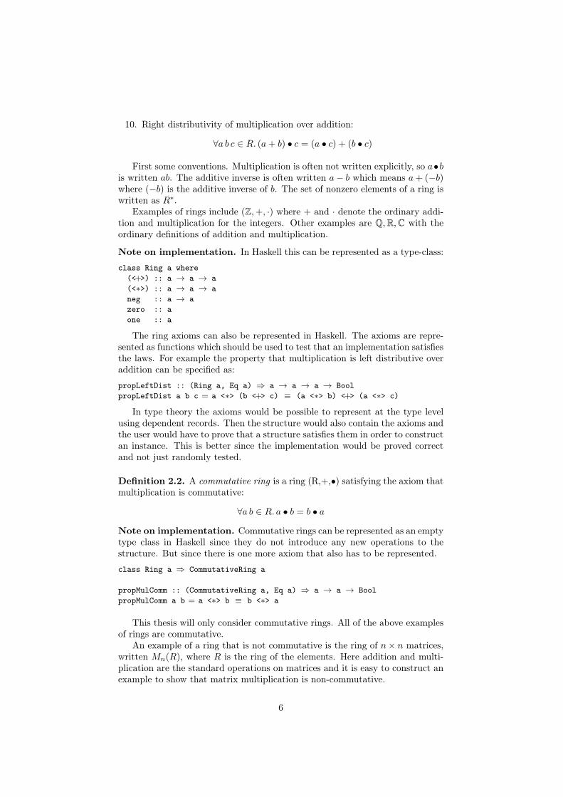
10. Right distributivity of multiplication over addition:

∀a b c ∈ R. (a+ b) • c = (a • c) + (b • c)

First some conventions. Multiplication is often not written explicitly, so a•bis written ab. The additive inverse is often written a− b which means a+ (−b)where (−b) is the additive inverse of b. The set of nonzero elements of a ring iswritten as R∗.

Examples of rings include (Z,+, ·) where + and · denote the ordinary addi-tion and multiplication for the integers. Other examples are Q,R,C with theordinary definitions of addition and multiplication.

Note on implementation. In Haskell this can be represented as a type-class:

class Ring a where

(<+>) :: a → a → a

(<∗>) :: a → a → a

neg :: a → a

zero :: a

one :: a

The ring axioms can also be represented in Haskell. The axioms are repre-sented as functions which should be used to test that an implementation satisfiesthe laws. For example the property that multiplication is left distributive overaddition can be specified as:

propLeftDist :: (Ring a, Eq a) ⇒ a → a → a → Bool

propLeftDist a b c = a <∗> (b <+> c) ≡ (a <∗> b) <+> (a <∗> c)

In type theory the axioms would be possible to represent at the type levelusing dependent records. Then the structure would also contain the axioms andthe user would have to prove that a structure satisfies them in order to constructan instance. This is better since the implementation would be proved correctand not just randomly tested.

Definition 2.2. A commutative ring is a ring (R,+,•) satisfying the axiom thatmultiplication is commutative:

∀a b ∈ R. a • b = b • a

Note on implementation. Commutative rings can be represented as an emptytype class in Haskell since they do not introduce any new operations to thestructure. But since there is one more axiom that also has to be represented.

class Ring a ⇒ CommutativeRing a

propMulComm :: (CommutativeRing a, Eq a) ⇒ a → a → Bool

propMulComm a b = a <∗> b ≡ b <∗> a

This thesis will only consider commutative rings. All of the above examplesof rings are commutative.

An example of a ring that is not commutative is the ring of n× n matrices,written Mn(R), where R is the ring of the elements. Here addition and multi-plication are the standard operations on matrices and it is easy to construct anexample to show that matrix multiplication is non-commutative.

6

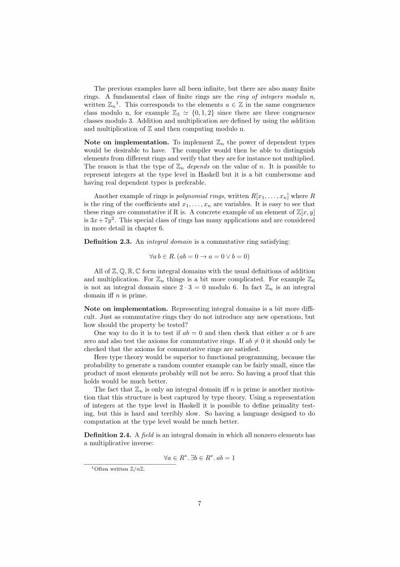
The previous examples have all been infinite, but there are also many finiterings. A fundamental class of finite rings are the ring of integers modulo n,written Zn

1. This corresponds to the elements a ∈ Z in the same congruenceclass modulo n, for example Z3 ≃ {0, 1, 2} since there are three congruenceclasses modulo 3. Addition and multiplication are defined by using the additionand multiplication of Z and then computing modulo n.

Note on implementation. To implement Zn the power of dependent typeswould be desirable to have. The compiler would then be able to distinguishelements from different rings and verify that they are for instance not multiplied.The reason is that the type of Zn depends on the value of n. It is possible torepresent integers at the type level in Haskell but it is a bit cumbersome andhaving real dependent types is preferable.

Another example of rings is polynomial rings, written R[x1, . . . , xn] where Ris the ring of the coefficients and x1, . . . , xn are variables. It is easy to see thatthese rings are commutative if R is. A concrete example of an element of Z[x, y]is 3x+7y2. This special class of rings has many applications and are consideredin more detail in chapter 6.

Definition 2.3. An integral domain is a commutative ring satisfying:

∀a b ∈ R. (ab = 0 → a = 0 ∨ b = 0)

All of Z,Q,R,C form integral domains with the usual definitions of additionand multiplication. For Zn things is a bit more complicated. For example Z6

is not an integral domain since 2 · 3 = 0 modulo 6. In fact Zn is an integraldomain iff n is prime.

Note on implementation. Representing integral domains is a bit more diffi-cult. Just as commutative rings they do not introduce any new operations, buthow should the property be tested?

One way to do it is to test if ab = 0 and then check that either a or b arezero and also test the axioms for commutative rings. If ab 6= 0 it should only bechecked that the axioms for commutative rings are satisfied.

Here type theory would be superior to functional programming, because theprobability to generate a random counter example can be fairly small, since theproduct of most elements probably will not be zero. So having a proof that thisholds would be much better.

The fact that Zn is only an integral domain iff n is prime is another motiva-tion that this structure is best captured by type theory. Using a representationof integers at the type level in Haskell it is possible to define primality test-ing, but this is hard and terribly slow. So having a language designed to docomputation at the type level would be much better.

Definition 2.4. A field is an integral domain in which all nonzero elements hasa multiplicative inverse:

∀a ∈ R∗. ∃b ∈ R∗. ab = 1

1Often written Z/nZ.

7

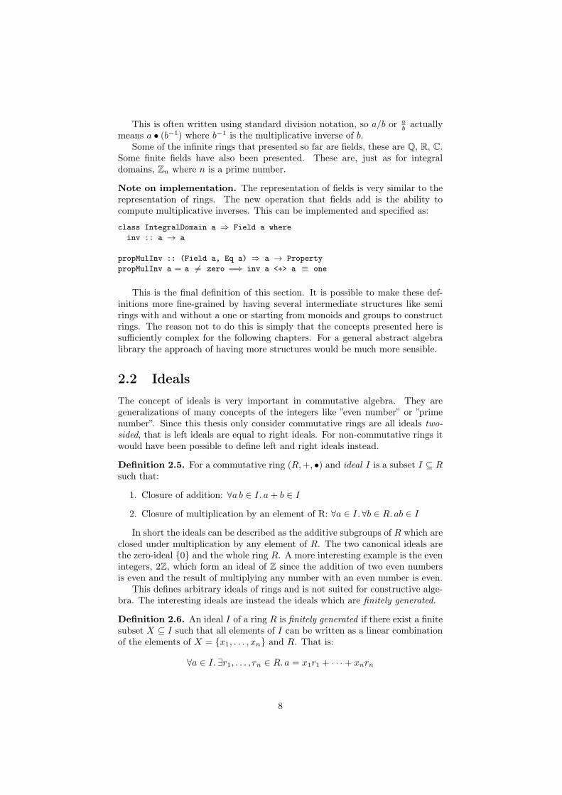
This is often written using standard division notation, so a/b or ab

actuallymeans a • (b−1) where b−1 is the multiplicative inverse of b.

Some of the infinite rings that presented so far are fields, these are Q, R, C.Some finite fields have also been presented. These are, just as for integraldomains, Zn where n is a prime number.

Note on implementation. The representation of fields is very similar to therepresentation of rings. The new operation that fields add is the ability tocompute multiplicative inverses. This can be implemented and specified as:

class IntegralDomain a ⇒ Field a where

inv :: a → a

propMulInv :: (Field a, Eq a) ⇒ a → Property

propMulInv a = a 6= zero =⇒ inv a <∗> a ≡ one

This is the final definition of this section. It is possible to make these def-initions more fine-grained by having several intermediate structures like semirings with and without a one or starting from monoids and groups to constructrings. The reason not to do this is simply that the concepts presented here issufficiently complex for the following chapters. For a general abstract algebralibrary the approach of having more structures would be much more sensible.

2.2 Ideals

The concept of ideals is very important in commutative algebra. They aregeneralizations of many concepts of the integers like ”even number” or ”primenumber”. Since this thesis only consider commutative rings are all ideals two-sided, that is left ideals are equal to right ideals. For non-commutative rings itwould have been possible to define left and right ideals instead.

Definition 2.5. For a commutative ring (R,+, •) and ideal I is a subset I ⊆ Rsuch that:

1. Closure of addition: ∀a b ∈ I. a+ b ∈ I

2. Closure of multiplication by an element of R: ∀a ∈ I. ∀b ∈ R. ab ∈ I

In short the ideals can be described as the additive subgroups of R which areclosed under multiplication by any element of R. The two canonical ideals arethe zero-ideal {0} and the whole ring R. A more interesting example is the evenintegers, 2Z, which form an ideal of Z since the addition of two even numbersis even and the result of multiplying any number with an even number is even.

This defines arbitrary ideals of rings and is not suited for constructive alge-bra. The interesting ideals are instead the ideals which are finitely generated.

Definition 2.6. An ideal I of a ring R is finitely generated if there exist a finitesubset X ⊆ I such that all elements of I can be written as a linear combinationof the elements of X = {x1, . . . , xn} and R. That is:

∀a ∈ I. ∃r1, . . . , rn ∈ R. a = x1r1 + · · ·+ xnrn

8

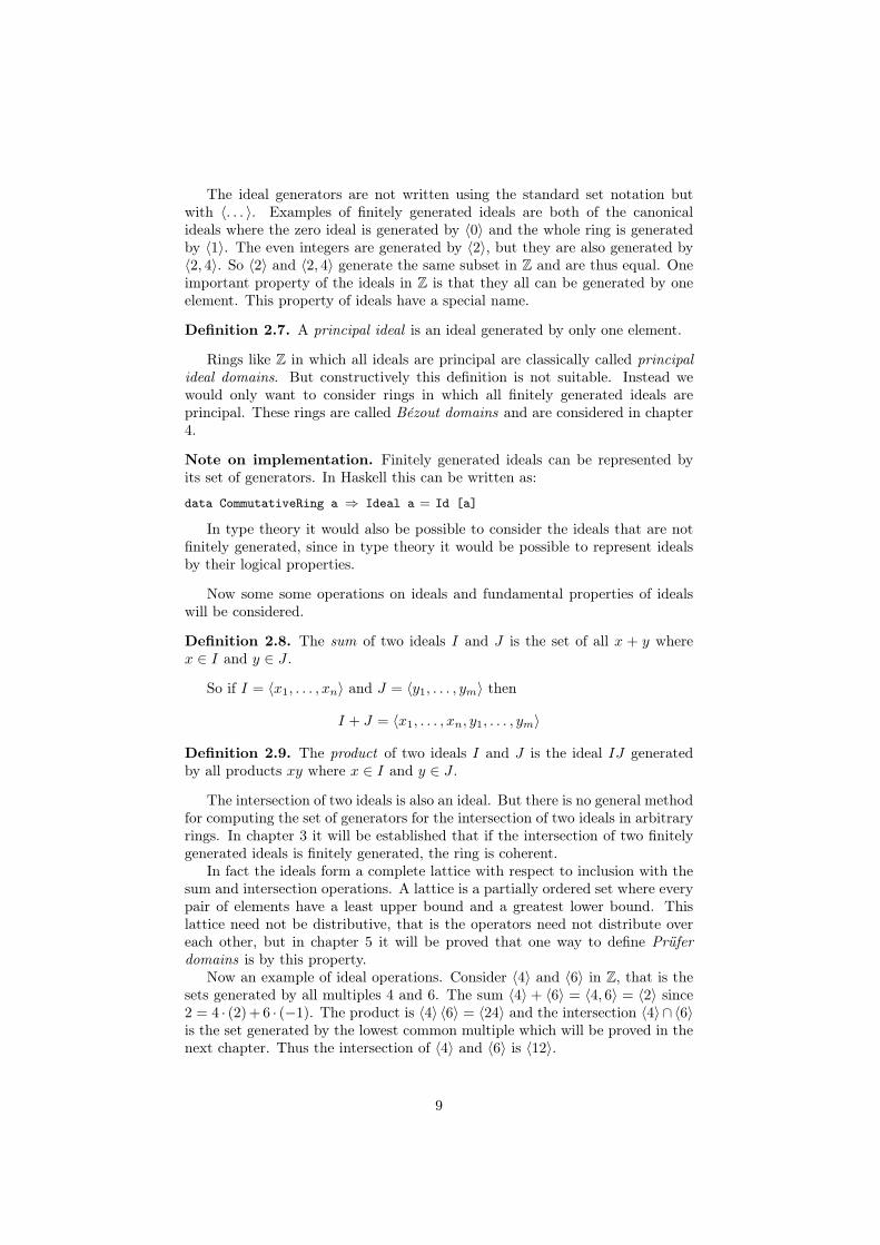
The ideal generators are not written using the standard set notation butwith 〈. . . 〉. Examples of finitely generated ideals are both of the canonicalideals where the zero ideal is generated by 〈0〉 and the whole ring is generatedby 〈1〉. The even integers are generated by 〈2〉, but they are also generated by〈2, 4〉. So 〈2〉 and 〈2, 4〉 generate the same subset in Z and are thus equal. Oneimportant property of the ideals in Z is that they all can be generated by oneelement. This property of ideals have a special name.

Definition 2.7. A principal ideal is an ideal generated by only one element.

Rings like Z in which all ideals are principal are classically called principalideal domains. But constructively this definition is not suitable. Instead wewould only want to consider rings in which all finitely generated ideals areprincipal. These rings are called Bézout domains and are considered in chapter4.

Note on implementation. Finitely generated ideals can be represented byits set of generators. In Haskell this can be written as:

data CommutativeRing a ⇒ Ideal a = Id [a]

In type theory it would also be possible to consider the ideals that are notfinitely generated, since in type theory it would be possible to represent idealsby their logical properties.

Now some some operations on ideals and fundamental properties of idealswill be considered.

Definition 2.8. The sum of two ideals I and J is the set of all x + y wherex ∈ I and y ∈ J .

So if I = 〈x1, . . . , xn〉 and J = 〈y1, . . . , ym〉 then

I + J = 〈x1, . . . , xn, y1, . . . , ym〉

Definition 2.9. The product of two ideals I and J is the ideal IJ generatedby all products xy where x ∈ I and y ∈ J .

The intersection of two ideals is also an ideal. But there is no general methodfor computing the set of generators for the intersection of two ideals in arbitraryrings. In chapter 3 it will be established that if the intersection of two finitelygenerated ideals is finitely generated, the ring is coherent.

In fact the ideals form a complete lattice with respect to inclusion with thesum and intersection operations. A lattice is a partially ordered set where everypair of elements have a least upper bound and a greatest lower bound. Thislattice need not be distributive, that is the operators need not distribute overeach other, but in chapter 5 it will be proved that one way to define Prüferdomains is by this property.

Now an example of ideal operations. Consider 〈4〉 and 〈6〉 in Z, that is thesets generated by all multiples 4 and 6. The sum 〈4〉 + 〈6〉 = 〈4, 6〉 = 〈2〉 since2 = 4 · (2)+6 · (−1). The product is 〈4〉 〈6〉 = 〈24〉 and the intersection 〈4〉 ∩ 〈6〉is the set generated by the lowest common multiple which will be proved in thenext chapter. Thus the intersection of 〈4〉 and 〈6〉 is 〈12〉.

9

2.3 Discrete and strongly discrete rings

This section will consider some rings that are especially relevant for constructivemathematics.

Definition 2.10. A ring is called discrete if equality is decidable.

All of the rings studied in the thesis will be discrete. But there are manyexamples of rings that are not discrete. For example R is not discrete since it isnot possible to decide if two irrational numbers are equal in finite time. Anotherexample of rings that do not need to be discrete are formal power series rings;rings of polynomials with and infinite number of terms.

Definition 2.11. A ring is called strongly discrete if ideal membership is de-cidable.

This property is very strong. Many of the rings we have seen so far arestrongly discrete, this is in fact tightly connected to whether division is decidablein the ring. In section 3.2 we will see that strong discreteness and coherencegive us the possibility of solving arbitrary systems of the type AX = B.

2.4 Noetherian rings and Dedekind domains

This section will establish some classical notions that will play an importantrôle throughout the thesis.

Definition 2.12. A ring is called Noetherian if every ideal is finitely generated.

This notion is not suitable for constructive mathematics since it relies onquantification over arbitrary subsets of the ring. It is not possible to formulatein first-order logic [4]. One of the goals of this thesis is to consider structuresthat are non-Noetherian analogues to classical notions.

Definition 2.13. A Dedekind domain is an integral domain in which everyfractional ideal is invertible.

An ideal is invertible if there exists another ideal such that the productof the ideals is principal. Dedekind domains imply Noetherianity and is thusnot suitable for constructive mathematics. Instead one consider Prüfer domainswhich are non-Noetherian analogues of Dedekind domains. These and invertibleideals will be considered in chapter 5.

10

Chapter 3

Coherent rings

All rings in this section are integral domains. One of the main aims of thefollowing sections will be to prove that different rings are coherent. That meansthat it is possible to solve systems of equations in them.

3.1 Definition and properties

An elementary application of linear algebra is to solve systems of linear equa-tions in many variables. But in linear algebra the central concept of study isvector spaces which implies that the underlying structures are fields. So whencomputing the solution of a system of equations one is free to use the assumptionthat the elements are invertible. But what happens if you drop the assumptionof invertibility and just look at integral domains? This is one of the motivationsto study coherence.

Definition 3.1. A ring R is coherent if every finitely generated ideal is finitelypresented. This means that given a matrix M ∈ R1×n there exist a matrixL ∈ Rn×m for m ∈ N such that ML = 0 and

MX = 0 ↔ ∃Y ∈ Rm×1. X = LY

This means that it is possible to compute a set of generators for solutionsof equations in a coherent ring. In other words that the module of solution forMX = 0 is finitely generated.

Note on implementation. The property of coherence is quite hard to capturein Haskell. The content that can be captured is that it is possible to computethe matrix L given M such that ML = 0. This can be represented as:

class IntegralDomain a ⇒ Coherent a where

solve :: Vector a → Matrix a

propCoherent :: (Coherent a, Eq a) ⇒ Vector a → Bool

propCoherent m = isSolution m (solve m)

Here isSolution just check that all elements in the product ML are zero. Thelogical aspects of coherence is harder to represent. But in type theory this wouldbe possible and it would be interesting to see what this would give compared towhat the Haskell approach gives.

11

Not only is it possible to solve equations in a coherent ring, but in fact itis possible to compute generators for any homogeneous system of equations ina coherent ring. The proof of this proposition is a translation of the proof ofproposition 1.2 in [18].

Proposition 3.2. In a coherent ring it is possible to solve a system MX = 0where M ∈ Rm×n and X ∈ Rn×1.

Proof. Let Mi ∈ R1×n be the rows of M . By coherence it is possible to solveM1X = 0 and get L1 ∈ Rn×p1 such that

M1X = 0 ↔ ∃Y ∈ Rp1×1. X = L1Y

Now replace X in M2X = 0 by L1Y and get M2L1Y = 0. By coherence we nowobtain a new matrix L2 ∈ Rp1×p2 such that

M1X = M2X = 0 ↔ ∃Y ∈ Rp1×1. X = L1Y and M2L1Y = 0

↔ ∃Z ∈ Rp2×1. X = L1L2Z

By iterating this method the solution X = L1L2 . . . LmZ with Li ∈ Rpi−1×pi ,p0 = n and Z ∈ Rpm×1 can be computed.

Now we will consider the intersection of finitely generated ideals in coherentrings. This gives another way of characterizing coherent rings in terms of theintersection of ideals. For the more general formulation of this in terms ofmodules, that is vector spaces over arbitrary rings and not just fields, seetheorem 2.4 on page 82 in [16].

Proposition 3.3. The intersection of two finitely generated ideals in a coherentring R is finitely generated.

Proof. Let I = 〈a1, . . . , an〉 and J = 〈b1, . . . , bm〉 be two finitely generated idealsin R. Consider the system

AX −BY = 0

where A is the 1×n matrix (a1, . . . , an) and B is the 1×m matrix (b1, . . . , bm).Since the ring is coherent it is possible to compute a finite number of generators(X1, Y1), . . . , (Xp, Yp) of the solution. This mean

AX1 = BY1

...

AXp = BYp

To say that α ∈ I ∩ J means that α ∈ I ∧ α ∈ J . This means that thereexist xi and yi such that α = a1x1 + · · · + anxn and α = b1y1 + · · · + bmym.Which means that a1x1+ · · ·+ anxn = b1y1+ · · ·+ bmym which is exactly whatthe generators above give. Thus are one set of generators for the intersectionAX1, . . . , AXp and another set of generators are BY1, . . . , BYp.

In fact this statement can be turned around to give the other direction also.The following proposition is the most important in this section and all of thecoherence proofs will rely on this.

12

Proposition 3.4. If R is an integral domain such that the intersection of twofinitely generated ideals is finitely generated then R is coherent.

Proof. The proof is by induction on the length of the system to solve. Firstconsider

ax = 0

Here the only solution is the trivial solution. Now assume that it is possibleto solve a system in n− 1 variables and consider the case with n ≥ 2 variables:

a1x1 + . . .+ anxn = 0

If a1 = 0 one set of solutions to the system is generated by (1, 0, . . . , 0),but it is also possible to use the induction hypothesis and get the generatorsvi2, . . . , vin for the system with x2, . . . , xn and the solutions of the system withn unknowns are generated by (0, vi2, . . . , vin) and (1, 0, . . . , 0).

If a1 6= 0 the set (0, vi2, . . . , vin) of solutions can be found by the inductionhypothesis again. Further, by hypothesis it is possible to find t1, . . . , tp suchthat

〈a1〉 ∩ 〈−a2, . . . ,−an〉 = 〈t1, . . . tp〉where ti = a1wi1 = −a2wi2 − . . .− anwin. So if a1x1 + . . .+ anxn = 0 then

a1x1 = −a2x2 − . . .− anxn. We also have ui such that

a1x1 = −a2x2 − . . .− anxn =

p∑

i=1

uiti

This implies that a1x1 =∑p

i=1 uiti =∑p

i=1 uia1wi1 which by the cancella-tion property give that x1 =

∑pi=1 uiwi1. Similarly

−a2x2 − . . .− anxn =

p∑

i=1

uiti =

p∑

i=1

ui(−a2wi2 − . . .− anwin)

Some reorganization gives

a2

(

x2 −p∑

i=1

uiwi2

)

+ . . .+ an

(

xn −p∑

i=1

uiwin

)

= 0

This gives that (wi1, . . . , win) and (0, vi2, . . . , vin) generate the module ofsolution.

This gives a method for proving that rings are coherent. Now the ”only” thingto prove is how to compute the intersection of finitely generated ideals andthen this will imply that the ring is coherent. This also shows that coherentrings can be characterized only in terms of the intersection of finitelygenerated ideals.

Note on implementation. One thing worth emphasizing here is the depen-dence on the witnesses of the intersection. That is given two finitely generatedideals I = 〈x1, . . . , xn〉 and J = 〈y1, . . . , yn〉 the functions that compute the in-tersection must also give a set of witnesses. If the intersection I∩J = 〈z1, . . . , zl〉then the function should give aij and bij such that

zk = ak1x1 + . . .+ aknxn

= bk1y1 + . . .+ bkmym

13

Note that this only gives the witnesses in one direction, that is if x ∈ I ∩ Jthen x ∈ I and x ∈ J .

3.2 Coherence and strongly discrete rings

The property of strong discreteness is very strong (as indicated by the name).If the ring is strongly discrete and coherent, not only is it possible to solvesystems like MX = 0 but it is also possible to solve general systems of the kindMX = A. For ideal membership to be decidable constructively there has to bea method to test if x ∈ 〈x1, . . . , xn〉 which also should give a witness if this isthe case. The witness should be a list of wi such that

∑

i wixi = x. In otherwords, it should be possible to write x as a linear combination of the wi.

Proposition 3.5. If R is a strongly discrete coherent integral domain then itis possible to solve arbitrary linear systems. Given MX = A it is possible tocompute X0 and L such that ML = 0 and

MX = A ↔ ∃Y.X = LY +X0

Proof. The solution L to the system MX = 0 can be computed by proposition3.2. The particular solution X0 can be computed using the same method as inthat proof. The base case when M has only one row is clear since R is stronglydiscrete. That is if M = (x1, . . . , xn) and A = (a) then the decidability ofideal membership give that if a ∈ 〈x1, . . . , xn〉 one get witnesses wi such thatx1w1 + · · ·+ xnwn = a.

This section establishes the properties of the rings to be studied throughoutthe thesis. One of the goals of the rest of the thesis is to give constructive proofsthat different rings are coherent. This means that in the end there will be manyexamples of rings in which it is possible to solve systems of linear equations.

14

Chapter 4

Bézout domains

This section will consider a class of integral domains called Bézout domains.These are non-Noetherian analogues of principal ideal domains. Examples ofBézout domains are Z and k[x]. The goal of this section is to give some moti-vation and examples of Bézout domains and then prove that they are coherent.Finally there will be some discussion on what is required for them to be stronglydiscrete.

4.1 Definition

One interesting class of integral domains is principal ideal domains, that areintegral domains in which all ideals are principal. This means that all principalideal domains are Noetherian, but as mentioned in chapter 2 is Noetherianitynot suitable for constructive mathematics. Thus are principal ideal domains notsuitable and we instead introduce Bézout domains.

Definition 4.1. An integral domain R is a Bézout domain iff every finitelygenerated ideal is principal.

Note on implementation. This definition means that it is possible to com-pute t such that 〈a1, . . . , an〉 = 〈t〉. The method should also compute witnessesthat 〈a1, . . . , an〉 ⊆ 〈t〉 and 〈a1, . . . , an〉 ⊇ 〈t〉. This can be represented in Haskellas

class IntegralDomain a ⇒ BezoutDomain a where

toPrincipal :: Ideal a → (Ideal a,[a],[a])

Here the first list is the witness that there exists ui such that

t = a1u1 + · · ·+ anun

The second list is the witness that there exists vi for each ai such that

ai = tvi

15

4.2 Euclidean domains

Many examples of Bézout domains are Euclidean domains. These are rings withadditional structure, namely an Euclidean function. This allows a generalizationof the Euclidean algorithm on integers.

Definition 4.2. An Euclidean domain is an integral domain R with a functionf : R∗ → N with the property that for a, b ∈ R there exist q, r ∈ R such thata = bq + r where either r = 0 or f(r) < f(b).

Euclidean domains are integral domains where it is possible to perform divi-sion with remainder. Examples include Z with the absolute value function andthe ring of polynomials k[x] with the degree function.

In order to show that Euclidean domains are Bézout domains some lemmasare needed. In Euclidean domains the Euclidean algorithm for computing thegreatest common divisor of two elements can be applied. There is a generalizedversion which computes the greatest common divisor of more than two elements.

Lemma 4.3. The generalized greatest common divisor (ggcd) of n elements canbe computed by recursively applying the algorithm for computing the gcd of twoelements. More specifically:

ggcd(a1, . . . , an) = gcd(a1, gcd(a2, . . . gcd(an−1, an) . . . ))

Proof. Consider the case with a, b, c ∈ R. Let d = ggcd(a, b, c) then we havethat d|b and d|c by the definition of gcd, so gcd(b, c) = kd for some k. We alsohave that d|a, so a = jd for some j. Now let u = gcd(k, j), by the constructionof u we have that ud|a, b, c, but since d is the greatest common divisor u mustbe a unit. Thus d = gcd(a, gcd(b, c)). By induction the other cases followdirectly.

In Euclidean domains it is also possible to compute the extended Euclideanalgorithm; given a, b ∈ R it is possible to compute x, y ∈ R such that ax+ by =gcd(a, b). This algorithm can also be generalized.

Lemma 4.4. Given a1, . . . , an ∈ R it is possible to compute x1, . . . , xn ∈ Rsuch that a1x1 + · · ·+ anxn = ggcd(a1, . . . , an)

Proof. Given a, b, c ∈ R we want to compute x, y, z ∈ R such that ax+by+cz =ggcd(a, b, c). We can compute m,n ∈ R such that bm + cn = gcd(b, c). Thenthere are l, k ∈ R such that ak+ gcd(b, c) · l = gcd(a, gcd(b, c)) which by lemma4.3 is equal to ggcd(a, b, c). So we get that ak + bml + cnl = ggcd(a, b, c) andthus x = k, y = ml and z = nl. The equations for more than three variablesfollow by induction.

Now it is possible to show that all Euclidean domains are Bézout domains.This gives a rich source of examples of Bézout domains.

Proposition 4.5. Euclidean domains are Bézout domains.

Proof. Follow directly from lemma 4.4. Given 〈a1, . . . , an〉 we can computet = ggcd(a1, . . . , an) such that t = a1x1 + · · · + anxn and thus we have that〈a1, . . . , an〉 = 〈ggcd(a1, . . . , an)〉.

16

Note on implementation. The implementation of this proof will have tocompute the witnesses also. One direction follow directly from the proof sincethe extended Euclidean algorithm is used. The other direction is also directsince division is decidable and t divides all ai.

4.3 Coherence of Bézout domains

The coherence of Bézout domains can be proved by considering the intersectionof ideals. Since all finitely generated ideals are principal it is sufficient to consideronly principal ideals.

Proposition 4.6. Given two ideals I = 〈a〉 and J = 〈b〉 the intersection isI ∩ J = 〈lcm(a, b)〉. Where lcm is the lowest common multiple of a and b.

Proof. The equality is proved by considering both inclusions.⊆: If f ∈ 〈a〉 ∩ 〈b〉 then f ∈ 〈a〉 and f ∈ 〈b〉. So a|f and b|f . But there

exist a lowest common multiple of a and b, lcm(a, b), such that a|lcm(a, b) andb|lcm(a, b) so f must be a multiple of the lowest common multiple and thusf ∈ 〈lcm(a, b)〉.

⊇: If f ∈ 〈lcm(a, b)〉 then lcm(a, b)|f . Since lcm(a, b) is a multiple of botha and b f must be a multiple of a and b also. This means that f ∈ 〈a〉∩ 〈b〉.

This is what we need in order to know that Bézout domains are coherent.

Theorem 4.7. Bézout domains are coherent.

Proof. Direct consequence of propositions 3.4 and 4.6.

Note on implementation. The implementation of this proof relies on thecomputation of the witnesses. Again it is sufficient to only consider the casewhere the ideals are principal. Given a and b we should compute lcm(a, b), uand v such that

lcm(a, b) = au

lcm(a, b) = bv

using the knowledge that we can compute gcd(a, b) = g, u1, u2, v1 and v2such that

g = au1 + bu2

a = gv1

b = gv2

To compute lcm(a, b) use that

lcm(a, b) =ab

gcd(a, b)

So lcm(a, b) can be computed as

lcm(a, b) = gv1v2 = g

(

a

g· bg

)

=ab

g(∗)

17

Now that the lowest common multiple has been computed the witnesses hasto be computed. But this is easy since by (∗) we get that

u = bg= v2

v = ag= v1

4.4 Bézout domains and strong discreteness

Recall that a ring is called strongly discrete if ideal membership is decidable.In order to decide ideal membership for Bézout domains we need to be able todecide divisibility.

Proposition 4.8. A Bézout domain R is strongly discrete if division is decid-able in R.

Proof. To test if x ∈ 〈x1, . . . , xn〉 we need to find wi such that x =∑

wixi.Since R is a Bézout domain we can find g such that 〈g〉 = 〈x1, . . . , xn〉.

Now, since divisibility is decidable, test if g|x and if this is the case weknow that x ∈ 〈g〉. This should also give us q such that x = qg and since〈g〉 ⊆ 〈x1, . . . , xn〉 we have ui such that g =

∑

uixi.The witness that x ∈ 〈x1, . . . , xn〉 can now be computed by

x = qg = q∑

uixi =∑

(qui)xi

and thus wi = qui.

This means that we can solve arbitrary linear systems MX = A for Bézoutdomains with decidable division and in particular over Z and k[x].

4.5 GCD domains and fields of fractions

In classical mathematics a structure that is studied is called unique factorizationdomains (UFD) which are integral domains in which all elements can be writtenuniquely as a product of irreducible elements. For example Z is an UFD by thefundamental theorem of arithmetic. But as for principal ideal domains (PIDs)this relies on Noetherianity. In classical mathematics we have the followingchain of inclusions.

Euclidean domains ⊂ PIDs ⊂ UFDs ⊂ Integral domains

But without the Noetherian assumption we get Bézout domains instead ofPIDs. One can show that an integral domain in which any two nonzero elementshave a greatest common divisor is a non-Noetherian analogue of the UFDs.These rings are called greatest common divisor (GCD) domains and completethe corresponding chain of inclusions in constructive mathematics.

Euclidean domains ⊂ Bézout domains ⊂ GCD domains ⊂ Integral domains

The inclusion Bézout domains ⊂ GCD domains is easy to see. But note thatnot all GCD domains are coherent.

18

One reason to look at GCD domains is that they provide a good setting inwhich to implement the field of fractions for an integral domain. As the nameindicates it is a field in which the integral domain can be embedded.

Definition 4.9. The field of fractions of an integral domain R is the set ofequivalence classes of pairs (a, s) where a, s ∈ R and s 6= 0 under the equivalencerelation:

(a, s) ≡ (b, t) iff at = bs

An integral domain can be embedded by the map a 7→ (a, 1). Addition andmultiplication can be defined as

(a, s) + (b, t) = (at+ bs, st)

(a, s)(b, t) = (ab, st)

The inverse of (a, s) where a, s 6= 0 is (s, a). It is easy to verify that this satisfiesthe conditions for a field.

The equivalence classes can be viewed as fractions. Thus is the constructionof fields of fractions a generalization of the construction of Q from Z to arbitraryintegral domains. Another special construction is the field of fractions for k[x](k discrete field) which is called the field of rational functions and is denotedby k(x). This is the field where the elements are fractions of polynomials in onevariable which will be important in section 5.5.2 when looking at an exampleof a Prüfer domains that is not a Bézout domains. This can be generalized tomultivariate polynomials and one then get the field of rational functions of apolynomial ring k[x1, . . . , xn] denoted by k(x1, . . . , xn).

The reason that GCD domains are a good setting for constructing the field offractions is that it is possible to restrict the equivalence classes to those in whichgcd(a, b) = 1. So all fractions will be in normal form. This is a generalizationof the fact that 4

2 can be simplified to 12 in Q to arbitrary fields of fractions.

Note on implementation. To implement GCD domains just follow the usualmethod without forgetting the witnesses. Given nonzero a, b ∈ R we shouldcompute gcd(a, b), x and y such that

a = gcd(a, b)x

b = gcd(a, b)y

1 = gcd(x, y)

This makes it very easy to represent the field of fractions over a GCD domain.It can be represented by a pair where the second element always should benonzero.

The reduction to normal form of a pair (a, b) works by computing gcd(a, b)and if it is 1 everything is fine. If it is not equal to 1 then return (x, y).

Using this it is trivial to implement Q with the help of a suitable imple-mentation of Z and if one also have an implementation of k[x] it is trivial toimplement k(x). This method could be used as a basis for implementing therational numbers in type theory. For instance this is how it is implemented inthe C-CORN library mentioned in the section on previous work.

19

In this section we have seen that Bézout domains are coherent and givensome examples of them. But the assumption that all finitely generated idealsare principal is quite strong and there are many examples of coherent rings inwhich this assumption does not hold. The next section will look at a superset ofBézout domains that also are coherent. These rings are called Prüfer domainsand there will be some examples of Prüfer domains that are not Bézout domainsfor which it is not clear that it is possible to solve systems of equations over.

20

Chapter 5

Prüfer domains

This chapter describes another class of coherent rings called Prüfer domains.First one of the many characterizations of Prüfer domains will be presentedfollowed by some constructions leading up to the coherence proof. Next therewill be some examples of what can be done in terms of ideal arithmetic in Prüferdomains and finally there will be some examples of Prüfer domains that are notBézout domains. This whole section follow [8, 18].

5.1 Definition

The classical definition of Prüfer domains is that they are non-Noetherian gen-eralization of Dedekind domains. Just as Bézout domains inherit many proper-ties from principal ideal domains Prüfer domains inherit many properties fromDedekind domains. A first observation is that Prüfer domains allow many dif-ferent classifications concerning aspects like: localization, structural and arith-metical properties of ideals and polynomial rings. The classification that willbe considered in this thesis is a simple first-order condition.

Definition 5.1. An integral domain R is a Prüfer domain iff

∀x y. ∃u v w. ux = vy ∧ (1− u)y = wx (∗)

Note on implementation. As for the other algebraic structures this can berepresented in the Haskell type class system as

class IntegralDomain a ⇒ PruferDomain a where

calcUVW :: a → a → (a,a,a)

propCalcUVW :: (PruferDomain a, Eq a) ⇒ a → a → Bool

propCalcUVW x y = u <∗> x ≡ v <∗> y && (one <-> u) <∗> y ≡ w <∗> x

where (u,v,w) = calcUVW x y

In type theory this would be possible to represent as a dependent record withthe properties as part of the structure.

A commutative ring satisfying (∗) is called arithmetical. In fact many proper-ties can be proved at the level of arithmetical rings (discussed further in [8, 18]).

As mentioned above are Bézout domains a subset of Prüfer domains. Thefollowing proposition will give a way of finding examples Prüfer domains.

21

Proposition 5.2. Bézout domains are Prüfer domains.

Proof. Since we have Bézout domain we can compute g, a and b such that

g = gcd(x, y)

x = ag

y = bg

We can also compute c and d such that

ca+ db = 1

Now let u = db . Then we shall find v such that

dbx = vy

Which simplifies todbag = vbg

Takev = ad

Now we want to compute w such that

wx = (1− u)y

= (1− db)y

= cay

= cagb

Since x = ag we get thatw = bc

Now we have found u, v and w satisfying the Prüfer condition and thus theproof is complete.

Now that we have found a source of examples of Prüfer domains we willcontinue to look at some useful constructions possible in Prüfer domains whichwill lead to the coherence proof.

5.2 Principal localization matrices

A key concept in the proof of coherence for Prüfer domains are principal local-ization matrices.

Definition 5.3. A principal localization matrix for a finitely generated ideal〈x1, . . . , xn〉 is a matrix A = (aij) such that

{

∑

aii = 1

aljxi = alixj ∀i, j, l ∈ {1, . . . , n}

Before considering how to compute the principal localization matrix in aPrüfer domain first consider how to do it for the simpler case of Bézout domains.

22

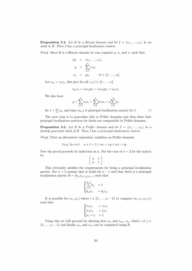
Proposition 5.4. Let R be a Bézout domain and let I = 〈x1, . . . , xn〉 be anideal in R. Then I has a principal localization matrix.

Proof. Since R is a Bézout domain we can compute g, ui and vi such that

〈g〉 = 〈x1, . . . , xn〉

g =n∑

i=1

xiui

xi = gvi ∀i ∈ {1, . . . , n}

Let aij = uivj , this give for all i, j, l ∈ {1, . . . , n}

aljxi = ulvjgvi = ulvigvj = alixj

We also have

g =

n∑

i=1

xiui =

n∑

i=1

gviui = g

n∑

i=1

aii

So 1 =∑

aii and thus (aij) is principal localization matrix for I.

The next step is to generalize this to Prüfer domains and thus show thatprincipal localization matrices for ideals are computable in Prüfer domains.

Proposition 5.5. Let R be a Prüfer domain and let I = 〈x1, . . . , xn〉 be afinitely generated ideal of R. Then I has a principal localization matrix.

Proof. First an alternative equivalent condition on Prüfer domains

∀x y. ∃u v w t. u+ t = 1 ∧ ux = vy ∧ wx = ty

Now the proof proceeds by induction on n. For the case of n = 2 let the matrixbe

[

u vw t

]

This obviously satisfies the requirements for being a principal localizationmatrix. For n > 2 assume that it holds for n − 1 and thus there is a principallocalization matrix B = (bij)1≤i,j≤n−1 such that

n−1∑

i=1

bii = 1

bljxi = blixj

It is possible for (xi, xn) where i ∈ {1, . . . , n − 1} to compute (ui, vi, wi, ti)such that

uixn = vixi

wixn = tixi

ui + ti = 1

Using this we will proceed by showing how aii and ann, aij where i 6= j ∈{1, . . . , n− 1} and finally ani and ain can be computed using B.

23

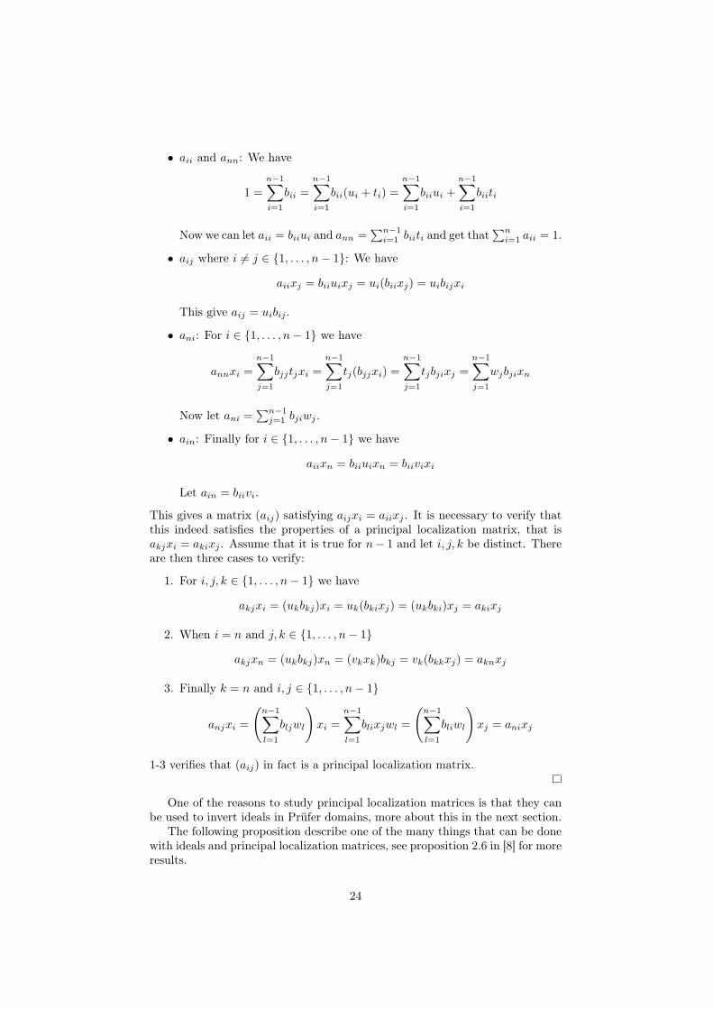
• aii and ann: We have

1 =

n−1∑

i=1

bii =

n−1∑

i=1

bii(ui + ti) =

n−1∑

i=1

biiui +

n−1∑

i=1

biiti

Now we can let aii = biiui and ann =∑n−1

i=1 biiti and get that∑n

i=1 aii = 1.

• aij where i 6= j ∈ {1, . . . , n− 1}: We have

aiixj = biiuixj = ui(biixj) = uibijxi

This give aij = uibij .

• ani: For i ∈ {1, . . . , n− 1} we have

annxi =n−1∑

j=1

bjjtjxi =n−1∑

j=1

tj(bjjxi) =

n−1∑

j=1

tjbjixj =

n−1∑

j=1

wjbjixn

Now let ani =∑n−1

j=1 bjiwj .

• ain: Finally for i ∈ {1, . . . , n− 1} we have

aiixn = biiuixn = biivixi

Let ain = biivi.

This gives a matrix (aij) satisfying aijxi = aiixj . It is necessary to verify thatthis indeed satisfies the properties of a principal localization matrix, that isakjxi = akixj . Assume that it is true for n− 1 and let i, j, k be distinct. Thereare then three cases to verify:

1. For i, j, k ∈ {1, . . . , n− 1} we have

akjxi = (ukbkj)xi = uk(bkixj) = (ukbki)xj = akixj

2. When i = n and j, k ∈ {1, . . . , n− 1}

akjxn = (ukbkj)xn = (vkxk)bkj = vk(bkkxj) = aknxj

3. Finally k = n and i, j ∈ {1, . . . , n− 1}

anjxi =

(

n−1∑

l=1

bljwl

)

xi =

n−1∑

l=1

blixjwl =

(

n−1∑

l=1

bliwl

)

xj = anixj

1-3 verifies that (aij) in fact is a principal localization matrix.

One of the reasons to study principal localization matrices is that they canbe used to invert ideals in Prüfer domains, more about this in the next section.

The following proposition describe one of the many things that can be donewith ideals and principal localization matrices, see proposition 2.6 in [8] for moreresults.

24

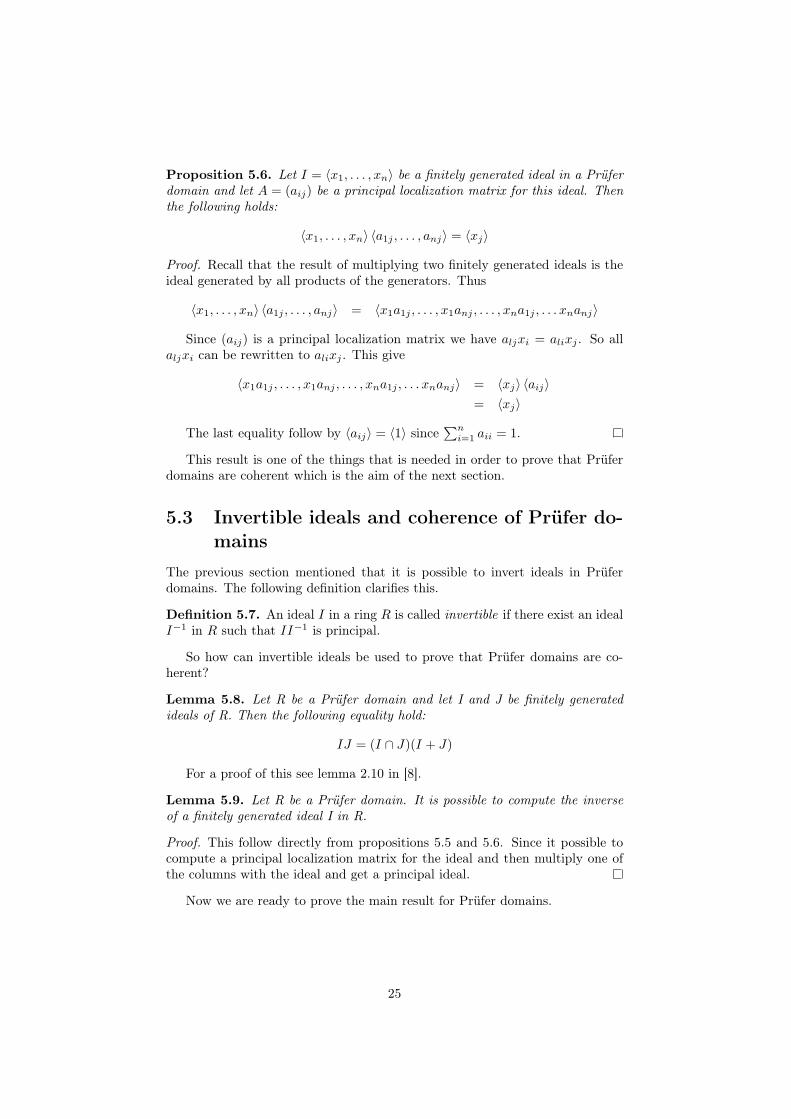
Proposition 5.6. Let I = 〈x1, . . . , xn〉 be a finitely generated ideal in a Prüferdomain and let A = (aij) be a principal localization matrix for this ideal. Thenthe following holds:

〈x1, . . . , xn〉 〈a1j , . . . , anj〉 = 〈xj〉

Proof. Recall that the result of multiplying two finitely generated ideals is theideal generated by all products of the generators. Thus

〈x1, . . . , xn〉 〈a1j , . . . , anj〉 = 〈x1a1j , . . . , x1anj , . . . , xna1j , . . . xnanj〉

Since (aij) is a principal localization matrix we have aljxi = alixj . So allaljxi can be rewritten to alixj . This give

〈x1a1j , . . . , x1anj , . . . , xna1j , . . . xnanj〉 = 〈xj〉 〈aij〉= 〈xj〉

The last equality follow by 〈aij〉 = 〈1〉 since∑n

i=1 aii = 1.

This result is one of the things that is needed in order to prove that Prüferdomains are coherent which is the aim of the next section.

5.3 Invertible ideals and coherence of Prüfer do-

mains

The previous section mentioned that it is possible to invert ideals in Prüferdomains. The following definition clarifies this.

Definition 5.7. An ideal I in a ring R is called invertible if there exist an idealI−1 in R such that II−1 is principal.

So how can invertible ideals be used to prove that Prüfer domains are co-herent?

Lemma 5.8. Let R be a Prüfer domain and let I and J be finitely generatedideals of R. Then the following equality hold:

IJ = (I ∩ J)(I + J)

For a proof of this see lemma 2.10 in [8].

Lemma 5.9. Let R be a Prüfer domain. It is possible to compute the inverseof a finitely generated ideal I in R.

Proof. This follow directly from propositions 5.5 and 5.6. Since it possible tocompute a principal localization matrix for the ideal and then multiply one ofthe columns with the ideal and get a principal ideal.

Now we are ready to prove the main result for Prüfer domains.

25

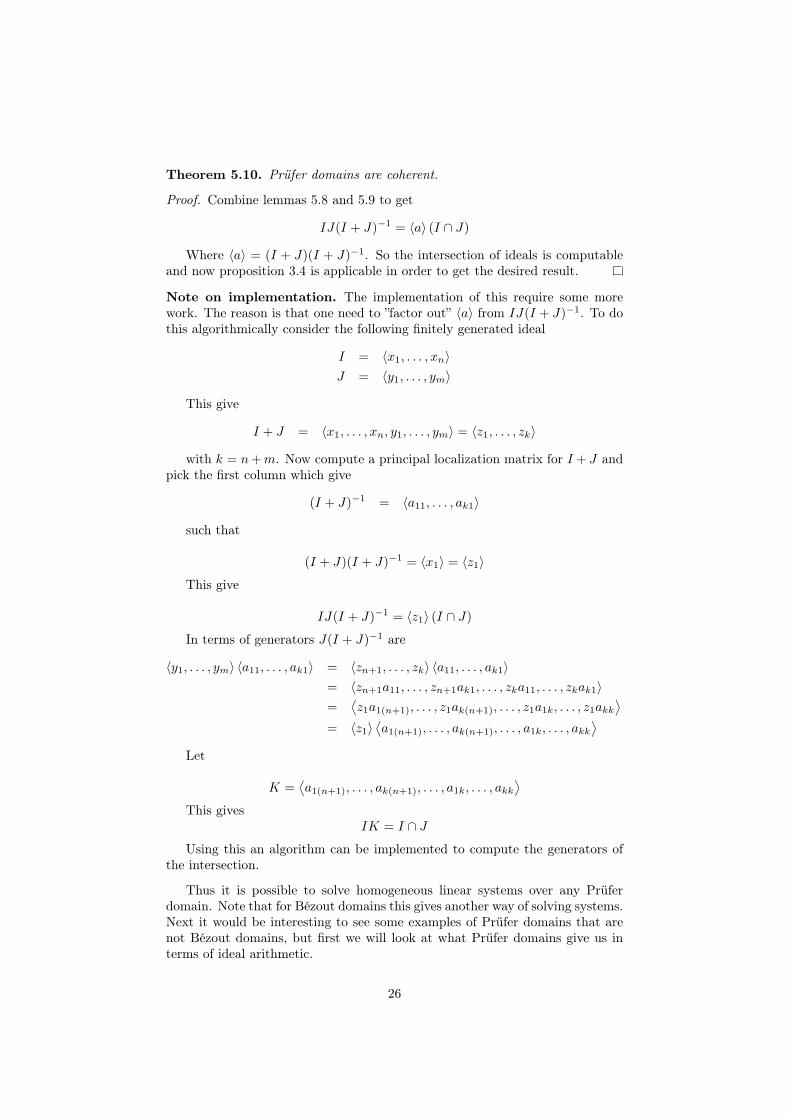
Theorem 5.10. Prüfer domains are coherent.

Proof. Combine lemmas 5.8 and 5.9 to get

IJ(I + J)−1 = 〈a〉 (I ∩ J)

Where 〈a〉 = (I + J)(I + J)−1. So the intersection of ideals is computableand now proposition 3.4 is applicable in order to get the desired result.

Note on implementation. The implementation of this require some morework. The reason is that one need to ”factor out” 〈a〉 from IJ(I + J)−1. To dothis algorithmically consider the following finitely generated ideal

I = 〈x1, . . . , xn〉J = 〈y1, . . . , ym〉

This give

I + J = 〈x1, . . . , xn, y1, . . . , ym〉 = 〈z1, . . . , zk〉

with k = n+m. Now compute a principal localization matrix for I + J andpick the first column which give

(I + J)−1 = 〈a11, . . . , ak1〉

such that

(I + J)(I + J)−1 = 〈x1〉 = 〈z1〉This give

IJ(I + J)−1 = 〈z1〉 (I ∩ J)

In terms of generators J(I + J)−1 are

〈y1, . . . , ym〉 〈a11, . . . , ak1〉 = 〈zn+1, . . . , zk〉 〈a11, . . . , ak1〉= 〈zn+1a11, . . . , zn+1ak1, . . . , zka11, . . . , zkak1〉=

⟨

z1a1(n+1), . . . , z1ak(n+1), . . . , z1a1k, . . . , z1akk⟩

= 〈z1〉⟨

a1(n+1), . . . , ak(n+1), . . . , a1k, . . . , akk⟩

Let

K =⟨

a1(n+1), . . . , ak(n+1), . . . , a1k, . . . , akk⟩

This givesIK = I ∩ J

Using this an algorithm can be implemented to compute the generators ofthe intersection.

Thus it is possible to solve homogeneous linear systems over any Prüferdomain. Note that for Bézout domains this gives another way of solving systems.Next it would be interesting to see some examples of Prüfer domains that arenot Bézout domains, but first we will look at what Prüfer domains give us interms of ideal arithmetic.

26

5.4 Ideal arithmetic

Recall the definition of a lattice. A lattice is a partially ordered set where everypair of elements has a lowest upper bound (join) and a greatest lower bound(meet). For more information on this see any basic book on algebra, for example[9]. For finitely generated ideals we have that the join of two ideals correspondto the sum of them and the meet is the intersection, so the set of ideals in aPrüfer domain form a lattice with ⊆.

For ideals I, J,K in a Prüfer domain the following property hold

I ∩ (J +K) = (I ∩ J) + (I ∩K)

So ∩ distributes over + and thus the set of ideals in a Prüfer domain forma distributive lattice. In fact this is one of the different ways to classify Prüferdomains that were mentioned in the beginning of this chapter. For a proof thatthis property is sufficient to be a Prüfer domain see theorem 1.1 in [10].

Another interesting property of the ideals in Prüfer domains is that theysatisfy the cancellation property. That is given finitely generated ideals I, J,K,if

IJ = IK

then J = K or I = 0.

5.5 Examples of Prüfer domains

The proposition to be proved will give a way to find Prüfer domains that arenot Bézout domains. First some definitions are necessary.

Definition 5.11. Let B be a ring and A a subring of B. An element x ∈ B iscalled integral over A if it satisfies an equation of the form

xn + a1xn−1 + · · ·+ a1x+ an = 0

where ai ∈ A.

The elements of B that are integral over A form a subring of B, for a proofof this see corollary 5.3 in [1]. This ring is called the integral closure of A in B.

This is what is necessary in order to formulate the following important result.

Proposition 5.12. Let R be a Bézout domain and L an algebraic extension ofits field of fractions K. The integral closure S of R inside L is a Prüfer domain.

Proof. Let x, y ∈ R be nonzero and integral over R. The element

s =x

y

is integral over K and hence satisfies an equation on the form

a0sn + a1s

n−1 + · · ·+ an = 0 (∗)

with a0, . . . , an ∈ R. Since R is a Bézout domain it is safe to assume that〈a0, . . . , an〉 = 1. The first step is to show that the following elements are in S,i.e. show that they are integral over R. First a0s ∈ S since

(a0s)n + a0a1(a0s)

n−1 + · · ·+ an0an = 0

27

So aos+ a1 ∈ S also. Now (∗) can be rewritten as

(aos+ a1)sn−1 + · · ·+ an = 0

It follows that (a0s+ a1)s ∈ S. This process can be repeated and finally weget that

a0, a0s, a0s+ a1, (a0s+ a1)s, (a0s+ a1)s+ a2, . . .

are all in S. Thus we have in S

〈a0, a0s, a0s+ a1, (a0s+ a1)s, (a0s+ a1)s+ a2, . . . 〉 = 〈a0, . . . , an〉 = 1

This means that there exists m0,m1, . . . such that

m0a0 +m1a0s+m2(a0s+ a1) +m3(a0s+ a1)s+ · · · = 1

The final step in the proof is to find u, v, w such that{

ux = vy

(1− u)y = wx

Let

u = m0a0 +m2(a0s+ a1) + . . .

This give

(m0a0 +m2(a0s+ a1) + . . . )x = vy

So we can let v = us. Finally we have

1− u = m1a0s+m3(a0s+ a1)s+ . . .

= s(m1a0 +m3(a0s+ a1) + . . . )

This give (1− u)y = x(m1a0 +m3(a0s+ a1) + . . . ) and thus

w = m1a0 +m3(a0s+ a1) + . . .

Both the proposition and the proof are quite abstract. To make this moreconcrete we will consider two examples of rings which are not Bézout domainsbut can be shown to be Prüfer domains using the method just described. Thefirst example is an extension of the integers and the second is an algebraic curve.

5.5.1 Z[√−5]

This is the set where all elements are of the type a + b√−5 where a, b ∈ Z.

This ring is an example of an quadratic integer ring. These has been studied bynumber theorists for a long time, since quadratic integers are related to manyimportant problems in number theory, for example Fermat’s last theorem.

Addition and multiplication can be defined as

(a+ b√−5) + (c+ d

√−5) = (a+ c) + (b+ d)

√−5

(a+ b√−5)(c+ d

√−5) = (ac− 5bd) + (ad+ bc)

√−5

It is easy to verify that this forms a ring. To see that it is not a Bézoutdomain we need to find a finitely generated ideal that is not principal.

28

Proposition 5.13. The ideal generated by⟨

2, 1 +√−5⟩

in Z[√−5] is not prin-

cipal.

Proof. Assume that it is generated by a single element, that is 〈x〉 =⟨

2, 1 +√−5⟩

.

Let x = a+b√−5 and y = a−b

√−5 such that xy divide both 4 and (1+

√−5)(1−√

−5) = 1− (√−5)2 = 6. Thus xy|2, but xy = a2 + 5b2 = 2 is impossible. This

means that xy = 1 and thus x = 1 or x = −1.But 〈1〉 6=

⟨

2, 1 +√−5⟩

which means that⟨

2, 1 +√−5⟩

cannot be generatedby a single element.

The proof that Z[√−5] is a Prüfer domain follow proposition 5.12. The

reason that the proof is so verbose is that this hopefully will clarify the proofof proposition 5.12.

Proposition 5.14. Z[√−5] is a Prüfer domain.

Proof. Given x and y the goal is to compute u, v, w such that

{

ux = vy

(1− u)y = wx

Let a, b, c, d ∈ Z∗. Start with

s =a+ b

√−5

c+ d√−5

=(a+ b

√−5)(c− d

√−5)

c2 + 5d2

Now s can be written on the form s = p+ q√−5 where p, q ∈ Q and

p =ac+ 5bd

c2 + 5d2

q =bc− ad

c2 + 5d2

We have

s = p+ q√−5 ⇒ s− p = q

√−5

⇒ (s− p)2 = −5q2

⇒ s2 − 2sp+ p2 + 5q2 = 0

If we write this out with p and q we get

s2 − 2(ac+ 5bd)

c2 + 5d2s+

a2 + 5b2

c2 + 5d2= 0

Rewrite to a0s2 + a1s + a2 = 0 where a0, a1, a2 ∈ Z. We can assume that

〈a0, a1, a2〉 = 〈1〉 since we can always divide with ggcd(a0, a1, a2) to get this.By the same reasoning as in the proof of proposition 5.12 we get that

〈a0, a0s, a0s+ a1, (a0s+ a1)s〉 = 〈1〉

29

So we can find m0,m1,m2,m3 such that

m0a0 +m1a0s+m2(a0s+ a1) +m3(a0s+ a1)s = 1

This give

u = m0a0 +m2(a0s+ a1)

v = m0a0s+m2(a0s+ a1)s

w = m1a0 +m3(a0s+ a1)

Note on implementation. Z[√−5] can be represented in Haskell as a pair

where the first element correspond to a and the second to b in a+ b√−5. The

proof that the ring is a Prüfer domain follow proposition 5.14 and is straightforward to implement now that most of the details has been worked out.

One important thing to keep in mind is that s lies in the field of fractions andthus the type of s is different from the type of, for instance, a0. So to performthe computations some conversions has to be made. First, elements has to beembedded into the field of fractions. Then, elements has to be extracted andthe extraction should only be possible if the divisor is 1. But since the prooftells us that all of a0s, a0s+ a1, (a0s+ a1)s lie in the integral closure of Z[

√−5]

this is not a problem.

5.5.2 k[x, y] with y2 = 1− x4

This ring correspond to an algebraic curve where all elements are of the forma+ b

√1− x4 with a, b ∈ k[x].

Addition and multiplication can be defined as

(a+ b√

1− x4) + (c+ d√

1− x4) = (a+ c) + (b+ d)√

1− x4

(a+ b√

1− x4)(c+ d√

1− x4) = (ac+ bd(1− x4)) + (ad+ bc)√

1− x4

Again the proof that this is a Prüfer domain follow proposition 5.12.

Proposition 5.15. k[x, y] with y2 = 1− x4 is a Prüfer domain.

Proof. Let a, b, c, d be nonzero elements of k[x]. Start with

s =a+ b

√1− x4

c+ d√1− x4

=(a+ b

√1− x4)(c− d

√1− x4)

c2 − d2(1− x4)

=ac− bd(1− x4) + (bc− ad)

√1− x4

c2 − d2(1− x4)

Now s can be written on the form s = p+ q√1− x4 where p, q ∈ k(x).

s2 − 2(ac− bd(1− x4))

c2 − d2(1− x4)s+

(ac− bd(1− x4))2 − (bc− ad)2(1− x4)

(c2 − d2(1− x4))2= 0

30

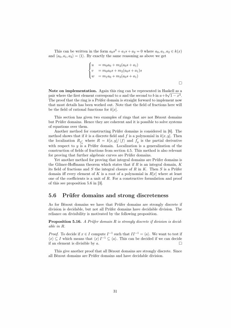
This can be written in the form a0s2 + a1s+ a2 = 0 where a0, a1, a2 ∈ k(x)

and 〈a0, a1, a2〉 = 〈1〉. By exactly the same reasoning as above we get

u = m0a0 +m2(a0s+ a1)

v = m0a0s+m2(a0s+ a1)s

w = m1a0 +m3(a0s+ a1)

Note on implementation. Again this ring can be represented in Haskell as apair where the first element correspond to a and the second to b in a+b

√1− x4.

The proof that the ring is a Prüfer domain is straight forward to implement nowthat most details has been worked out. Note that the field of fractions here willbe the field of rational functions for k[x].

This section has given two examples of rings that are not Bézout domainsbut Prüfer domains. Hence they are coherent and it is possible to solve systemsof equations over them.

Another method for constructing Prüfer domains is considered in [6]. Themethod shows that if k is a discrete field and f is a polynomial in k[x, y]. Thenthe localization Rf

′

ywhere R = k[x, y]/ 〈f〉 and f

′

y is the partial derivative

with respect to y is a Prüfer domain. Localization is a generalization of theconstruction of fields of fractions from section 4.5. This method is also relevantfor proving that further algebraic curves are Prüfer domains.

Yet another method for proving that integral domains are Prüfer domains isthe Gilmer-Hoffmann theorem which states that if R is an integral domain, Kits field of fractions and S the integral closure of R in K. Then S is a Prüferdomain iff every element of K is a root of a polynomial in R[x] where at leastone of the coefficients is a unit of R. For a constructive formulation and proofof this see proposition 5.6 in [3].

5.6 Prüfer domains and strong discreteness

As for Bézout domains we have that Prüfer domains are strongly discrete ifdivision is decidable, but not all Prüfer domains have decidable division. Thereliance on divisibility is motivated by the following proposition.

Proposition 5.16. A Prüfer domain R is strongly discrete if division is decid-able in R.

Proof. To decide if x ∈ I compute I−1 such that II−1 = 〈a〉. We want to test if〈x〉 ⊆ I which means that 〈x〉 I−1 ⊆ 〈a〉. This can be decided if we can decideif an element is divisible by a.

This give another proof that all Bézout domains are strongly discrete. Sinceall Bézout domains are Prüfer domains and have decidable division.

31

The next chapter will study yet another class of rings which has many differ-ent applications, these are polynomial rings. There have been a small taste ofspecial polynomial rings in this chapter and the next chapter will consider themin general. Traditionally Dedekind domains has been of great interest in numbertheory while polynomial rings has been of interest in algebraic geometry.

32

Chapter 6

Polynomial rings

Let k be a discrete field. The set of all multivariate polynomials in n variableswith coefficient in k, written k[x1, . . . , xn], form a commutative ring. The mainaim of this section is to study this ring and eventually prove that it is coherent.

This text is mainly based on [7] and many proofs has been omitted andcan be found there. But some of the most important proofs in it relies on anonconstructive version of Dicksons lemma, so these proofs contains a gap froma constructive point of view. This is considered in greater detail in [15] and themain results of it is presented here in order to fill in the gaps.

6.1 Monomials and monomial orderings

In order to develop the theory of multivariate polynomials the theory of mono-mials and how to order them has to be considered. For example, what is thegreatest of x3y and x2y3 in k[x, y]? Later in the chapter we will see that manyalgorithms on polynomials will rely on the monomial ordering.

Definition 6.1. A monomial in x1, . . . , xn is a product of the form xα1

1 · . . . ·xαnn

where α1, . . . , αn ∈ N.

This can be simplified by just looking at α = (α1, . . . , αn) and letting xα =xα1

1 · . . . · xαnn . The total degree of a monomial α is |α| = α1 + . . . + αn.

Definition 6.2. A monomial ordering is any total relation > on Nn satisfying

1. If α > β and γ ∈ Nn then α+ γ > β + γ.

2. > is a well-ordering on Nn.

We can now define some different monomial orderings.

Definition 6.3. Lexicographical order : α >lex β if the left-most nonzero entryis positive in α− β ∈ Zn.

This is a very simple ordering and it works exactly as lexicographical orderingof words. This ordering can seem a bit weird. Consider for example x and y3z5

with x > y > z, then x >lex y3z5. The following ordering remedies this.

33

Definition 6.4. Graded lexicographical order : α >grlex β if

|α| > |β| , or |α| = |β| and α >lex β

Here the total degree of the monomials first decide which is the greatest andlexicographical ordering is used to break ties. The following ordering is a bitless intuitive, but can be more efficient when doing computations.

Definition 6.5. Graded reverse lexicographical order : α >grevlex β if

|α| > |β| , or |α| = |β|

and the right-most nonzero entry in α− β ∈ Zn is negative.

The last two orderings are best illustrated by an example. Consider x2z2

and xy2z. Since they have same total degree lexicographical ordering will haveto break the tie for graded lexicographical ordering, thus x2z2 >grlex xy2z. Butusing graded reverse lexicographical order it will be the other way around, soxy2z >grevlex x2z2.

Note on implementation. One way to represent monomials in Haskell is as alist of integers denoting α = (α1, . . . , αn). The ordering can then be representedas a phantom type in the type of monomials. The type class system can then beused to make the monomial type indexed by a certain ordering an instance of theOrd class. So for each ordering we will have a type of monomials with a specialOrd instance. This is an example where the Haskell type system captures themathematical definitions very well.

6.2 Polynomial rings

Using monomials we can now define what a polynomial is.

Definition 6.6. A polynomial f ∈ k[x1, . . . , xn] is a linear combination ofmonomials, that is

f =∑

α

aαxα, aα ∈ k

For example f = 3x3y2 + z4 + 12xz is a polynomial in Q[x, y, z]. The to-

tal degree of a polynomial is the monomial with maximum total degree withnonzero coefficient, for example deg(f) = 5. It is possible to prove that addi-tion and multiplication of polynomials can be defined in a way which satisfy theproperties of commutative rings. Next some terminology.

Definition 6.7. Let f =∑

α aαxα be a polynomial in k[x1, . . . , xn] and let >

be a monomial order. Then

1. The multidegree of f (with respect to >) is

multideg(f) = max(α ∈ Nn : aα 6= 0)

2. The leading coefficient of f is

LC(f) = amultideg(f)

34

3. The leading monomial of f is

LM(f) = xmultideg(f)

4. The leading term of f is

LT (f) = LC(f) · LM(f)

Let f = 3x3y2 + z4 + 12xz be a polynomial in Q[x, y, z] ordered with graded

lexicographical order. Then

multideg(f) = (3, 2, 0)

LC(f) = 3

LM(f) = x3y2

LT (f) = 3x3y2

As mentioned above it is possible to define have addition, subtraction andmultiplication with expected behavior, but what about division? The case formultivariate polynomials is quite different from the case of univariate poly-nomials for which the standard division algorithm is applicable. The goal ink[x1, . . . , xn] is to divide a polynomial f by a list of polynomials f1, . . . , fs suchthat

f = q1f1 + · · ·+ qnfn + r

with q1, . . . , qn, r ∈ k[x1, . . . , xn].

Theorem 6.8. Every f ∈ k[x1, . . . , xn] can be written as

f = q1f1 + · · ·+ qnfn + r

with qi, r ∈ k[x1, . . . , xn] and either r = 0 or r is a linear combination ofmonomials, none of which is divisible by LT (f1), . . . , LT (fn). We call r the re-mainder on division by f1, . . . , fn. Furthermore if qifi 6= 0 then multideg(f) ≥multideg(qifi).

There is a standard algorithm which is given in [7, 15]. Termination is provedconstructively in [15]. One important property of this is that uniqueness is notnecessary. For example, division of x2 by [x+ y, x] in k[x, y] give

x2 = (x− y)(x+ y) + 0 · x+ y2

but division of x² by [x, x+ y] give

x2 = x · x+ 0 · (x+ y) + 0

So the order of the divisors matter!

Note on implementation. The only thing that is difficult to represent inHaskell is the order and naming of the variables. One way would be to representthis at the type level using phantom types, but this is a bit cumbersome. Itwould be easier to represent with dependent types since this requires that thelanguage has types depending on values.

35

6.3 Properties of ideals in k[x1, . . . , xn]

In section 4.2 it is proved that all ideals in Euclidean domains are principal andthis especially hold for k[x]. But this does not hold for k[x1, . . . , xn] if n ≥ 2.

Consider for example the ideal generated by 〈x, y〉 in k[x, y]. If it were tobe generated by a single element then this element would have to divide both xand y. But then it must be a nonzero constant and the ideal contain no otherconstant than zero. Thus it is not possible for the ideal to be generated by asingle element.

From here on this section deviates from [7] and is instead based on [15]. Thereason for this is that [7] builds the theory leading up to the Hilbert basis theo-rem and the theory of Gröbner bases on a nonconstructive version of Dickson’slemma.

Definition 6.9. A poset (E,≤) is said to satisfy the ascending chain condition(ACC) if for every non decreasing sequence (un)n∈N in E there exists n ∈ N

such that un = un+1.

This definition is to be read constructively. This means that there exist aneffective method for computing n. Section 3.1 in [15] contains a motivationwhy it is so important that ACC is read and motivated constructively and notclassically.

The versions of Dickson’s lemma and the Hilbert basis theorem in [7] relieson a classical interpretation of ACC and are thus not valid constructively.

Theorem 6.10. (Constructive) Dickson’s lemma: The poset finitely generatedmonomial ideals in k[x1, . . . , xn], ordered with ⊆, satisfies ACC.

This can then be used to prove the termination of the Buchberger algorithmfor computing Gröbner bases. Another important application of this is in theproof of the Hilbert basis theorem.

Theorem 6.11. (Constructive) Hilbert basis theorem: The poset of finitelygenerated ideals of k[x1, . . . , xn], ordered with ⊆, satisfies ACC.

This shows that k[x1, . . . , xn] satisfies the constructive version of Noethe-rianity. That is the set of finitely generated ideals in the ring satisfies theconstructive ACC.

6.4 Gröbner bases

In this section Gröbner bases will be defined and then the Buchberger algorithmwhich computes a Gröbner basis for an ideal is presented.

Definition 6.12. Let I ⊂ k[x1, . . . , xn] be an ideal other than {0}. Then LT (I)is the set of leading terms of elements

LT (I) = {cxα : ∃f ∈ I with LT (f) = cxα}

and 〈LT (I)〉 is the ideal generated by the elements of LT (I).

36

Definition 6.13. A Gröbner basis of an ideal I ⊆ k[x1, . . . , xn] is a list ofgenerators g1, . . . , gm of the ideal such that for all f ∈ I the division of f byg1, . . . , gm leads to a zero remainder.

Gröbner bases are the ”well-behaved” ideals in k[x1, . . . , xn]. One importantproperty is that division no longer is dependent on the order of the divisors.

Definition 6.14. If f, g ∈ k[x1, . . . , xn]\{0} with multideg(f) = α and multideg(g) =β. Let γ = (γ1, . . . , γd) where γi = max(αi, βi). Now define:

• The lowest common multiple: lcm(α, β) = γ

• The S-polynomial of f and g:

S[f, g] =xγ

LT (f)f − xγ

LT (g)g

Note that the S-polynomials is constructed in a way such that leading termsshould be cancelled. This will be crucial to the algorithm for computing Gröbnerbases. This algorithm is the famous Buchberger algorithm.

Theorem 6.15. Let I = 〈f1, . . . , fs〉 be a nonzero polynomial ideal. Thena Gröbner basis for I can be constructed in a finite number of steps by thefollowing algorithm:

Input: I = (f1,...,fs)

Output: A Gröbner basis G = (g1,...,gt) for I

G := I

REPEAT

G’ := G

FOR each pair (p,q), p 6= q in G’ DO

S := remainder (S_poly(p,q)) G’

IF S 6= 0 THEN G := G ∪ {S}

UNTIL G = G’

Termination and correctness of this algorithm is proved constructively in[15]. The intuition behind the algorithm is that division with the generatorsof the Gröbner basis should be zero. The algorithm iteratively compute theremainder of the division of the S-polynomials with the generators of the basis.If the result of this is zero nothing need to be added, but if the result is nonzerothe remainder should be added to the basis. This will force the basis to divideall elements of the ideals.

This version of the algorithm is quite naive and it generates very large bases.A simple trick to reduce the size of the Gröbner basis is given by the followinglemma.

Lemma 6.16. Let G be a Gröbner basis for the polynomial ideal I. Let p ∈ Gbe a polynomial such that LT (p) ∈ 〈LT (G− {p})〉. Then G − {p} is also aGröbner basis for I.

Using this it is possible to define what a minimal Gröbner basis is.

37

Definition 6.17. A minimal Gröbner basis for a polynomial ideal I is a Gröbnerbasis such that

∀p ∈ G. (LC(p) = 1 ∧ LT (p) /∈ 〈LT (G− {p})〉)

By multiplying with constant terms all leading coefficients can be made 1and by applying lemma 6.16 a minimal Gröbner basis can be constructed.

Now consider an example, we saw earlier that division of x² by [x + y, x]in k[x, y] give different results depending on the order, so [x + y, x] does notform a Gröbner basis. Using the algorithm above together with the method forcomputing minimal Gröbner bases we get the generators [x, y] as a Gröbnerbasis for the ideal. It is clear that x2 divided by [x, y] will not depend on theorder of the divisors.

Note on implementation. In Haskell this is quite straight forward to imple-ment. But in type theory it would require more effort since all of the proofswould have to be formalized. This has been done using a combination of Agdaand Coq in [17].

Another thing worth emphasizing is that the algorithm presented is notoptimized in any way, so it will be unrealistic to use it on larger examples.A lot of effort has been put into optimizing the Buchberger algorithm. Oneapproach to optimize the algorithm is not to try all pairs of polynomials but tryto find the ”best” pairs, for more details see [13]. Some of the optimizations hasbeen implemented in Haskell in the HaskellForMaths library by David Amosmentioned in the section on previous work.

6.5 Coherence of k[x1, . . . , xn]

The proof of coherence will be proved as for Bézout domains and Prüfer domains,that is by considering the intersection of ideals. An alternative proof can befound in [15].

Definition 6.18. Let I be a finitely generated ideal in k[x1, . . . , xn]. The r:thelimination ideal of I is Ir = I ∩ k[xr+1, . . . , xn] where 1 ≤ r ≤ n.

The computation of elimination ideals can be done by choosing the lexico-graphical ordering with x1 > · · · > xn and computing a Gröbner basis for I.Then the generators containing any of the xl where l < r are thrown away.Using this the intersection can be computed using the following trick.

Proposition 6.19. Let I and J be ideals in k[x1, . . . , xn]. Then

I ∩ J = (tI + (1− t)J) ∩ k[x1, . . . , xn]

where t is greater than all x1, . . . , xn.

Now coherence follow directly.

Theorem 6.20. The polynomial ring k[x1, . . . , xn] is coherent.

Proof. Direct consequence of propositions 3.4 and 6.19.

38

Note on implementation. In order to be able to test that the generated idealis in fact the intersection witnesses has to be computed.

In order to modify the algorithm to compute these some bookkeeping needsto be done. At each time an element is added to the basis the algorithm wouldhave to store the witness that this can be written using the elements of theinitial ideal.

6.6 Strong discreteness of k[x1, . . . , xn]

This requires a version of the Buchberger algorithm that computes witnessesthat the basis generate the same ideal as the first ideal. Which means thatthe generators for the first ideal should be able to be expressed as a linearcombination of the Gröbner basis and vice-versa.

Theorem 6.21. k[x1, . . . , xn] is strongly discrete, that is we can test f ∈〈h1, . . . , hm〉 and find witnesses w1, . . . , wm such that

f = w1h1 + · · ·+ wmhm

Proof. We want to decide if f ∈ 〈h1, . . . , hm〉. To do this first compute a Gröb-ner basis 〈g1, . . . , gl〉 for 〈h1, . . . , hm〉. Then compute f/[g1, . . . , gl] = (qs, r), ifr 6= 0 then we know that f /∈ 〈h1, . . . , hm〉. But if r = 0 we want to compute awitness that this is in fact true.

What we have is q1, . . . , ql such that

f = q1g1 + · · ·+ qlgl

We also have a witness that 〈h1, . . . , hm〉 ⊇ 〈g1, . . . , gl〉 which consists ofa11, . . . , a1m, . . . , al1, . . . , alm such that

g1 = a11h1 + · · ·+ a1mhm

...

gm = al1h1 + · · ·+ almhm

To compute the witness insert this in the above expression for f

f = q1(a11h1 + · · ·+ a1mhm) +

...

ql(al1h1 + · · ·+ almhm)

= h1(q1a11 + · · ·+ qlal1) +

...

hm(q1a1m + · · ·+ qlalm)

39

The witnesses that f ∈ 〈h1, . . . , hm〉 are

w1 = q1a11 + · · ·+ qlal1...

wm = q1a1m + · · ·+ qlalm

This means that it is possible to solve arbitrary linear systems MX = Aover k[x1, . . . , xn].

40

Chapter 7

Conclusions

The aim of this chapter is to tie together all the previous chapters by looking atthe result of the implementation and showing some examples of computationsusing it. The results are discussed and finally further work and limitations ofthe implementation are considered.

7.1 Implementation

The definitions and proofs in this thesis have been implemented in Haskell,the implementation can be found at http://hackage.haskell.org/package/constructive-algebra. This section will give a short overview of what canbe done with this implementation and motivate some of the design choices.The algorithms has been implemented in the form of a library. One point ofimplementing it as a library is that a user easily can extend it by adding newalgorithms and examples of rings.

The library is organized in three sections presented here with the most gen-eral parts first. The most general part is the level of all algebraic structuresrepresented as type classes with QuickCheck properties to specify them. Thegeneral proofs or algorithms that hold for the different structures are also rep-resented at this level. For example are coherent rings together with the proofthat coherence implies that it is possible to solve systems of linear equations arerepresented at this level.

Next there is a part which contain general notions that are neither structuresnor instances of the structures. Examples include ideals and the constructionof fields of fractions.

Finally there is the most concrete part which are concrete instances of thestructures. The rings that has been implemented are Z, Zn, Z[

√−5], Q, k[x],

k(x), k[x, y] with y2 = 1− x4 and k[x1, . . . , xn]. All of these has been tested toverify the different QuickCheck properties for the structures that they imple-ment. This give some assurance that the implementation is in fact correct.

Both Q and k(x) has been implemented using the representation of fieldsof fractions. Using this the implementation become more or less trivial. Forexample the representation of Q looks like

type Q = FieldOfFractions Z

41

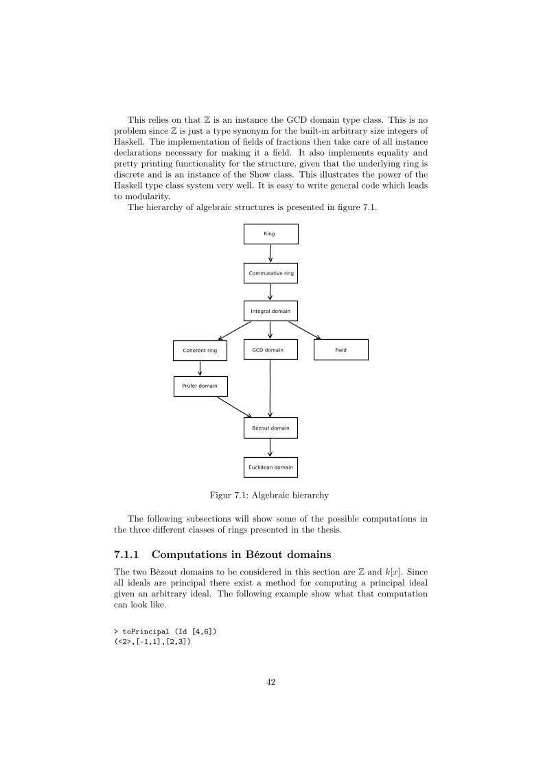
This relies on that Z is an instance the GCD domain type class. This is noproblem since Z is just a type synonym for the built-in arbitrary size integers ofHaskell. The implementation of fields of fractions then take care of all instancedeclarations necessary for making it a field. It also implements equality andpretty printing functionality for the structure, given that the underlying ring isdiscrete and is an instance of the Show class. This illustrates the power of theHaskell type class system very well. It is easy to write general code which leadsto modularity.

The hierarchy of algebraic structures is presented in figure 7.1.

Figur 7.1: Algebraic hierarchy

The following subsections will show some of the possible computations inthe three different classes of rings presented in the thesis.

7.1.1 Computations in Bézout domains

The two Bézout domains to be considered in this section are Z and k[x]. Sinceall ideals are principal there exist a method for computing a principal idealgiven an arbitrary ideal. The following example show what that computationcan look like.

> toPrincipal (Id [4,6])

(<2>,[-1,1],[2,3])

42

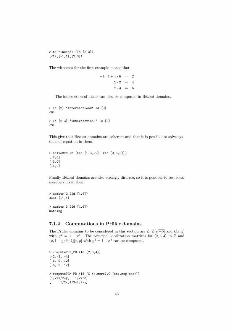
> toPrincipal (Id [2,3])

(<1>,[-1,1],[2,3])

The witnesses for the first example means that

−1 · 4 + 1 · 6 = 2

2 · 2 = 4

2 · 3 = 6

The intersection of ideals can also be computed in Bézout domains.

> Id [2] ‘intersectionB‘ Id [3]

<6>

> Id [2,3] ‘intersectionB‘ Id [3]

<3>

This give that Bézout domains are coherent and that it is possible to solve sys-tems of equation in them.

> solveMxN (M [Vec [1,3,-2], Vec [3,5,6]])

[ 7,0]

[-3,0]

[-1,0]

Finally Bézout domains are also strongly discrete, so it is possible to test idealmembership in them.

> member 2 (Id [4,6])

Just [-1,1]

> member 3 (Id [4,6])

Nothing

7.1.2 Computations in Prüfer domains

The Prüfer domains to be considered in this section are Z, Z[√−5] and k[x, y]

with y2 = 1 − x4. The principal localization matrices for 〈2, 3, 4〉 in Z and〈x, 1− y〉 in Q[x, y] with y2 = 1− x4 can be computed.

> computePLM_PD (Id [2,3,4])

[-2,-3, -4]

[-6,-9,-12]

[ 6, 9, 12]

> computePLM_PD (Id [C (x,zero),C (one,neg one)])

[1/2+1/2∗y, 1/2x^3][ 1/2x,1/2-1/2∗y]

43

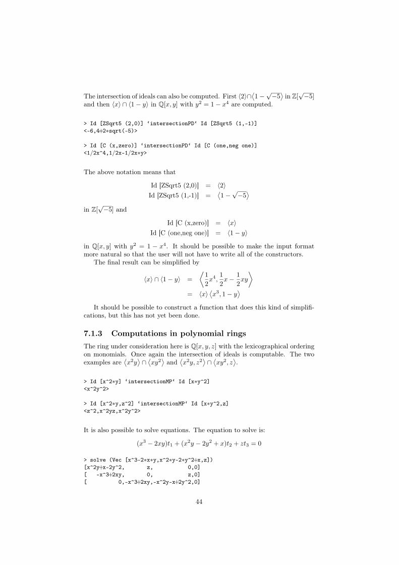
The intersection of ideals can also be computed. First 〈2〉∩⟨

1−√−5⟩

in Z[√−5]

and then 〈x〉 ∩ 〈1− y〉 in Q[x, y] with y2 = 1− x4 are computed.

> Id [ZSqrt5 (2,0)] ‘intersectionPD‘ Id [ZSqrt5 (1,-1)]

<-6,4+2∗sqrt(-5)>

> Id [C (x,zero)] ‘intersectionPD‘ Id [C (one,neg one)]

<1/2x^4,1/2x-1/2x∗y>

The above notation means that

Id [ZSqrt5 (2,0)] = 〈2〉Id [ZSqrt5 (1,-1)] =

⟨

1−√−5⟩

in Z[√−5] and

Id [C (x,zero)] = 〈x〉Id [C (one,neg one)] = 〈1− y〉

in Q[x, y] with y2 = 1 − x4. It should be possible to make the input formatmore natural so that the user will not have to write all of the constructors.

The final result can be simplified by

〈x〉 ∩ 〈1− y〉 =

⟨

1

2x4,

1

2x− 1

2xy

⟩

= 〈x〉⟨

x3, 1− y⟩

It should be possible to construct a function that does this kind of simplifi-cations, but this has not yet been done.

7.1.3 Computations in polynomial rings

The ring under consideration here is Q[x, y, z] with the lexicographical orderingon monomials. Once again the intersection of ideals is computable. The twoexamples are

⟨

x2y⟩

∩⟨

xy2⟩

and⟨

x2y, z2⟩

∩⟨

xy2, z⟩

.

> Id [x^2∗y] ‘intersectionMP‘ Id [x∗y^2]

<x^2y^2>

> Id [x^2∗y,z^2] ‘intersectionMP‘ Id [x∗y^2,z]

<z^2,x^2yz,x^2y^2>

It is also possible to solve equations. The equation to solve is:

(x3 − 2xy)t1 + (x2y − 2y2 + x)t2 + zt3 = 0

> solve (Vec [x^3-2∗x∗y,x^2∗y-2∗y^2+x,z])

[x^2y+x-2y^2, z, 0,0]

[ -x^3+2xy, 0, z,0]

[ 0,-x^3+2xy,-x^2y-x+2y^2,0]

44

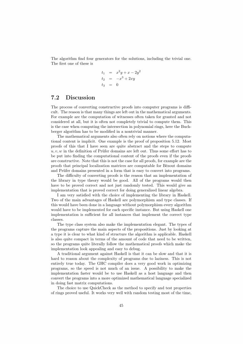
The algorithm find four generators for the solutions, including the trivial one.The first one of these is

t1 = x2y + x− 2y2

t2 = −x3 + 2xy

t3 = 0

7.2 Discussion

The process of converting constructive proofs into computer programs is diffi-cult. The reason is that many things are left out in the mathematical arguments.For example are the computation of witnesses often taken for granted and notconsidered at all, but it is often not completely trivial to compute them. Thisis the case when computing the intersection in polynomial rings, here the Buch-berger algorithm has to be modified in a nontrivial manner.

The mathematical arguments also often rely on notions where the computa-tional content is implicit. One example is the proof of proposition 5.12. Mostproofs of this that I have seen are quite abstract and the steps to computeu, v, w in the definition of Prüfer domains are left out. Thus some effort has tobe put into finding the computational content of the proofs even if the proofsare constructive. Note that this is not the case for all proofs, for example are theproofs that principal localization matrices are computable for Bézout domainsand Prüfer domains presented in a form that is easy to convert into programs.

The difficulty of converting proofs is the reason that an implementation ofthe library in type theory would be good. All of the programs would thenhave to be proved correct and not just randomly tested. This would give animplementation that is proved correct for doing generalized linear algebra.

I am very satisfied with the choice of implementing the library in Haskell.Two of the main advantages of Haskell are polymorphism and type classes. Ifthis would have been done in a language without polymorphism every algorithmwould have to be implemented for each specific instance. But using Haskell oneimplementation is sufficient for all instances that implement the correct typeclasses.

The type class system also make the implementation elegant. The types ofthe programs capture the main aspects of the propositions. Just by looking ata type it is clear to what kind of structure the algorithm is applicable. Haskellis also quite compact in terms of the amount of code that need to be written,so the programs quite literally follow the mathematical proofs which make theimplementation look appealing and easy to debug.

A traditional argument against Haskell is that it can be slow and that it ishard to reason about the complexity of programs due to laziness. This is notentirely true today. The GHC compiler does a very good work in optimizingprograms, so the speed is not much of an issue. A possibility to make theimplementation faster would be to use Haskell as a host language and thenconvert the programs into a more optimized mathematical language specializedin doing fast matrix computations.

The choice to use QuickCheck as the method to specify and test propertiesof rings proved useful. It works very well with random testing most of the time,

45

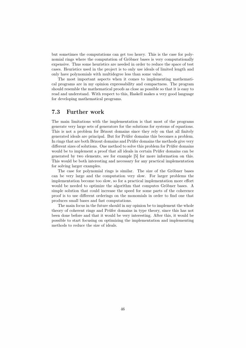
but sometimes the computations can get too heavy. This is the case for poly-nomial rings where the computation of Gröbner bases is very computationallyexpensive. Thus some heuristics are needed in order to reduce the space of testcases. Heuristics used in the project is to only use ideals of limited length andonly have polynomials with multidegree less than some value.

The most important aspects when it comes to implementing mathemati-cal programs are in my opinion expressability and compactness. The programshould resemble the mathematical proofs as close as possible so that it is easy toread and understand. With respect to this, Haskell makes a very good languagefor developing mathematical programs.

7.3 Further work

The main limitations with the implementation is that most of the programsgenerate very large sets of generators for the solutions for systems of equations.This is not a problem for Bézout domains since they rely on that all finitelygenerated ideals are principal. But for Prüfer domains this becomes a problem.In rings that are both Bézout domains and Prüfer domains the methods give verydifferent sizes of solutions. One method to solve this problem for Prüfer domainswould be to implement a proof that all ideals in certain Prüfer domains can begenerated by two elements, see for example [5] for more information on this.This would be both interesting and necessary for any practical implementationfor solving larger examples.

The case for polynomial rings is similar. The size of the Gröbner basescan be very large and the computation very slow. For larger problems theimplementation become too slow, so for a practical implementation more effortwould be needed to optimize the algorithm that computes Gröbner bases. Asimple solution that could increase the speed for some parts of the coherenceproof is to use different orderings on the monomials in order to find one thatproduces small bases and fast computations.

The main focus in the future should in my opinion be to implement the wholetheory of coherent rings and Prüfer domains in type theory, since this has notbeen done before and that it would be very interesting. After this, it would bepossible to start focusing on optimizing the implementation and implementingmethods to reduce the size of ideals.

46

Bibliography

[1] M. Atiyah and I. MacDonald. Introduction to commutative algebra.Addison-Wesley, 1969.

[2] Koen Claessen and John Hughes. Quickcheck: A Lightweight Tool for Ran-dom Testing of Haskell Programs. International Conference of FunctionalProgramming, 2000.

[3] Thierry Coquand. Space of Valuations, 2008. http://www.cse.chalmers.se/~coquand/val1.pdf.

[4] Thierry Coquand and Henri Lombardi. A logical approach to abstractalgebra. Math. Structures Comput. Sci, 16:885–900, 2006.

[5] Thierry Coquand, Henri Lombardi, and Claude Quitte. Generating non-Noetherian modules constructively. Manuscripta Mathematica, 115(4):513–520, 2004.

[6] Thierry Coquand, Henri Lombardi, and Claude Quitté. Curves and coher-ent Prüfer rings. 2009.

[7] David Cox, John Little, and Donal O’Shea. Ideals, Varieties and Algo-rithms: An introduction to Computational Algebraic Geometry and Com-mutative Algebra. Springer, 2006.

[8] L. Ducos, H. Lombardi, C. Quitté, and M. Salou. Théorie algorithmique desanneaux arithmétiques, des anneaux de Prüfer et des anneaux de Dedekind.Journal of Algebra, 281(2):604 – 650, 2004.

[9] John R. Durbin. Modern Algebra: An Introduction. Wiley, 2004.

[10] László Fuchs and Luigi Salce. Modules ofer Non-Noetherian Domains, vol-ume 84 of Mathematical Surveys and Monographs. American MathematicalSociety, 2001.

[11] François Garillot, Georges Gonthier, Assia Mahboubi, and LaurenceRideau. Packaging Mathematical Structures. In TPHOLs ’09: Proceed-ings of the 22nd International Conference on Theorem Proving in HigherOrder Logics, pages 327–342, Berlin, Heidelberg, 2009. Springer-Verlag.

[12] Herman Geuvers, Randy Pollack, Freek Wiedijk, and Jan Zwanenburg. AConstructive Algebraic Hierarchy in Coq. Journal of Symbolic Computa-tion, 34(4):271 – 286, 2002.

47

[13] Alessandro Giovini, Teo Mora, Gianfranco Niesi, Lorenzo Robbiano, andCarlo Traverso. "One sugar cube, please" or Selection strategies in theBuchberger algorithm. In Proceedings of the ISSAC’91, ACM Press, pages49–54, 1991.

[14] Georges Gonthier. Formal Proof – The Four-Color Theorem. Notices ofthe American Mathematical Society, 55(11), 2008.

[15] Henri Lombardi and Hervé Perdry. The Buchberger Algorithm as a Toolfor Ideal Theory of Polynomial Rings in Constructive Mathematics. 1998.

[16] Ray Mines, Fred Richman, and Wim Ruitenburg. A Course in ConstructiveAlgebra. Springer-Verlag, 1988.

[17] Henrik Persson. An Integrated Development of Buchberger’s Algorithm inCoq. 2001.

[18] Maïmouna Salou Idi Malam. Théorie Algorithmique des Anneaux Arith-métiques, des Anneaux de Prüfer et des Anneaux de Dedekind. PhD thesis,2002.

[19] A.S. Troelstra and D. van Dalen. Constructivism in Mathematics. North-Holland, 1988. 2 volumes.

48