Embed Size (px)
Citation preview
Contributions to Symbolicq-Hypergeometric Summation
Dissertationzur Erlangung des akademischen Grades
”Doktor der technischen Wissenschaften“
in der Studienrichtung Technische Mathematik
verfaßt von
Axel Riese
amForschungsinstitut fur symbolisches RechnenTechnisch-Naturwissenschaftliche Fakultat
Johannes Kepler Universitat Linz
November 1997
Erster Begutachter: a.o.Univ.-Prof. Dr. Peter PauleInstitut fur MathematikJ. Kepler Universitat Linz
Zweiter Begutachter: o.Univ.-Prof. Dr. Jochen PfalzgrafInstitut fur ComputerwissenschaftenUniversitat Salzburg

ii

iii
Eidesstattliche Erklarung
Ich versichere, daß ich die Dissertation selbstandig verfaßt habe, andere als die angegebe-nen Quellen und Hilfsmittel nicht verwendet und mich auch sonst keiner unerlaubten Hilfebedient habe.
Axel RieseLinz, im November 1997

iv
v
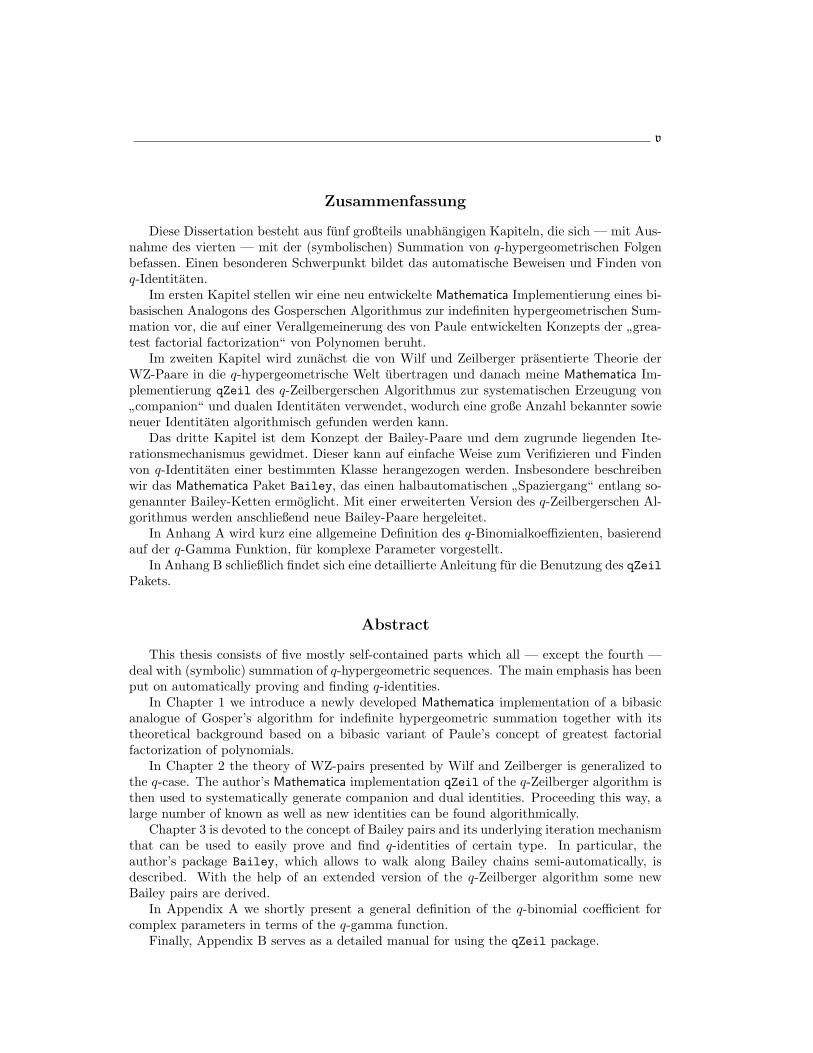
Zusammenfassung
Diese Dissertation besteht aus funf großteils unabhangigen Kapiteln, die sich — mit Aus-nahme des vierten — mit der (symbolischen) Summation von q-hypergeometrischen Folgenbefassen. Einen besonderen Schwerpunkt bildet das automatische Beweisen und Finden vonq-Identitaten.
Im ersten Kapitel stellen wir eine neu entwickelte Mathematica Implementierung eines bi-basischen Analogons des Gosperschen Algorithmus zur indefiniten hypergeometrischen Sum-mation vor, die auf einer Verallgemeinerung des von Paule entwickelten Konzepts der ”grea-test factorial factorization“ von Polynomen beruht.
Im zweiten Kapitel wird zunachst die von Wilf und Zeilberger prasentierte Theorie derWZ-Paare in die q-hypergeometrische Welt ubertragen und danach meine Mathematica Im-plementierung qZeil des q-Zeilbergerschen Algorithmus zur systematischen Erzeugung von
”companion“ und dualen Identitaten verwendet, wodurch eine große Anzahl bekannter sowieneuer Identitaten algorithmisch gefunden werden kann.
Das dritte Kapitel ist dem Konzept der Bailey-Paare und dem zugrunde liegenden Ite-rationsmechanismus gewidmet. Dieser kann auf einfache Weise zum Verifizieren und Findenvon q-Identitaten einer bestimmten Klasse herangezogen werden. Insbesondere beschreibenwir das Mathematica Paket Bailey, das einen halbautomatischen ”Spaziergang“ entlang so-genannter Bailey-Ketten ermoglicht. Mit einer erweiterten Version des q-Zeilbergerschen Al-gorithmus werden anschließend neue Bailey-Paare hergeleitet.
In Anhang A wird kurz eine allgemeine Definition des q-Binomialkoeffizienten, basierendauf der q-Gamma Funktion, fur komplexe Parameter vorgestellt.
In Anhang B schließlich findet sich eine detaillierte Anleitung fur die Benutzung des qZeilPakets.
Abstract
This thesis consists of five mostly self-contained parts which all — except the fourth —deal with (symbolic) summation of q-hypergeometric sequences. The main emphasis has beenput on automatically proving and finding q-identities.
In Chapter 1 we introduce a newly developed Mathematica implementation of a bibasicanalogue of Gosper’s algorithm for indefinite hypergeometric summation together with itstheoretical background based on a bibasic variant of Paule’s concept of greatest factorialfactorization of polynomials.
In Chapter 2 the theory of WZ-pairs presented by Wilf and Zeilberger is generalized tothe q-case. The author’s Mathematica implementation qZeil of the q-Zeilberger algorithm isthen used to systematically generate companion and dual identities. Proceeding this way, alarge number of known as well as new identities can be found algorithmically.
Chapter 3 is devoted to the concept of Bailey pairs and its underlying iteration mechanismthat can be used to easily prove and find q-identities of certain type. In particular, theauthor’s package Bailey, which allows to walk along Bailey chains semi-automatically, isdescribed. With the help of an extended version of the q-Zeilberger algorithm some newBailey pairs are derived.
In Appendix A we shortly present a general definition of the q-binomial coefficient forcomplex parameters in terms of the q-gamma function.
Finally, Appendix B serves as a detailed manual for using the qZeil package.

vi
vii
Contents
Introduction 1
1 A Generalization of Gosper’s Algorithm to Bibasic Hypergeometric Sum-mation 3
1.1 Theoretical Background 3
1.1.1 Bibasic Greatest Factorial Factorization 4
1.1.2 Bibasic Hypergeometric Telescoping 6
1.2 Degree Setting for Solving the Bibasic Key Equation 11
1.3 Applications 13
1.3.1 Bibasic Summation Formulas 14
1.3.2 Bibasic Matrix Inverses 15
1.3.3 Extensions and Open Problems 17
2 Automatic Generation of q-Identities 19
2.1 q-Hypergeometric Telescoping and qWZ-Certification 19
2.2 Companion Identities 22
2.3 Dual Identities 25
2.4 Applications 29
2.4.1 The q-Binomial Theorem 30
2.4.2 The Sum of a 1φ1 Series 31
2.4.3 The q-Chu-Vandermonde Identity 31
2.4.4 The Bailey-Daum Summation Formula 34
2.4.5 The q-Analogue of Bailey’s 2F1(−1) Sum 35
2.4.6 The q-Analogue of Gauss’ 2F1(−1) Sum 36
2.4.7 The q-Saalschutz Formula 37
2.4.8 The q-Dixon Formula 38
2.4.9 The Sum of a 6φ5 Series 39
2.4.10 Jackson’s q-Analogue of Dougall’s 7F6 Sum 40
2.4.11 Ramanujan’s Bilateral Sum 40
2.4.12 Bailey’s Sum of a 3ψ3 Series 40
3 Walking Along Bailey Chains 43
3.1 Basic Definitions and Tools 43
3.2 Bailey Pairs and Bailey Chains 44
3.2.1 Ordinary and Bilateral Bailey Pairs 44
3.2.2 Bailey Chains 46
3.3 From Bailey Chains to Bailey Lattices 52
3.3.1 Binomial Bailey Pairs 52
3.3.2 Dual Bailey Pairs 55
3.3.3 c-Step Bailey Pairs 57
viii CONTENTS
3.4 Slater’s Table of Bailey Pairs 613.5 Discovering New Bailey Pairs 64
A A Note on q-Binomial Coefficients 71
B How to Use qZeil 75B.1 Package Structure and Installation 75B.2 Interfaces 75B.3 The Summand 76B.4 The Summation Range 77B.5 The Optional Argument intconst 77B.6 Global Variables 77B.7 Options 78
B.7.1 Option EquationSolver 78B.7.2 Option OnlySummand 78B.7.3 Option MagicFactor 79B.7.4 Option Shadow 81B.7.5 Option FindAlphaBeta 81B.7.6 Option PolyMult 82
B.8 Additional Functions 88B.9 Speed-Up 88
Bibliography 90
Vita 95
1
Introduction
Thanks to Zeilberger’s [46] algorithm, proving most definite hypergeometric summation andtransformation formulas has become routine work that can be performed by a computer. Itwas also Zeilberger who first observed that his algorithm can be carried over to the q-hyper-geometric case. Based on Paule’s [32] algebraic concept of greatest factorial factorization(GFF), which provides an explanation of hypergeometric telescoping and extends beautifullyto the q- (and even multibasic) hypergeometric case, I implemented a Mathematica q-analogueof Zeilberger’s algorithm in the frame of my diploma thesis [37] trying to overcome short-comings of the already existing Maple implementations of Zeilberger (see Petkovsek, Wilf,and Zeilberger [36]) and Koornwinder [25]. Since I came up with a first prototype of qZeilin late 1993, the program has constantly undergone substantial improvements. Special at-tention has been directed to advancing the capabilities for finding q-identities automatically.As an example, qZeil now discovers polynomial multipliers or suggests powers of q whichmake a given input summable. This Extended q-Zeilberger Algorithm† builds the algorithmicbackbone of this thesis.
The thesis consists of five self-contained parts, which are all devoted to the field of q-seriesbut can mostly be read independently from each other. To this end some of the basicdefinitions appear more than once. Readers being familiar with the subject may safely skipthese repetitions.
In Chapter 1 a newly developed Mathematica implementation of a bibasic analogue ofGosper’s algorithm for indefinite hypergeometric summation is introduced together with itstheoretical background based on a bibasic variant of Paule’s [32] concept of greatest factorialfactorization of polynomials. This chapter has been already published in the ElectronicJournal of Combinatorics [38].
In Chapter 2 the theory of WZ-pairs developed by Wilf and Zeilberger [44] is gener-alized to the q-case. The author’s Mathematica implementation qZeil of the q-Zeilbergeralgorithm (cf. Paule and Riese [33]) is then used to systematically generate companion anddual identities from “standard” qWZ-pairs employing a recently established shadowing strat-egy. Proceeding this way, a large number of known as well as new identities can be foundautomatically.
In Chapter 3 it is shown how the concept of Bailey pairs and its underlying iterationmechanism (cf. Andrews [9,10] or Paule [30]) can be used to easily prove and find q-identitiesof certain type. In particular, the author’s package Bailey, which allows to walk along Baileychains semi-automatically, is described. With the help of qZeil some new Bailey pairs arederived.
In Appendix A we shortly present a general definition of the q-binomial coefficient forcomplex parameters in terms of the q-gamma function, which has been stimulated by several
†Latest information on the package can be retrieved via the World Wide Web from the qZeil homepageat http://www.risc.uni-linz.ac.at/research/combinat/risc/software/qZeil
2 INTRODUCTION
inaccurate definitions found in literature.Appendix B serves as a manual for the qZeil package including hints on installation,
usage, and new features.
Acknowledgements
Valuable contributions to the work on this thesis have been provided by the RISC combina-torics group. In particular I would like to thank
➠ my advisor Peter Paule for successfully spreading the q-disease and his extensive coop-eration and support,
➠ Christian “Malles” Mallinger for fruitful comments and friendship over the years,
➠ Markus Schorn and Erhard Aichinger for contributing parts of the code,
➠ Kurt Wegschaider, Istvan Nemes, and Roberto Pirastu for discussions, and
➠ Peter Stadelmeyer for being the PC-software guru.
I also thank my parents for supporting this project financially, as well as my family —Cornelia, Claudia, and Michaela — for sharing (q-) pleasure and frustration with me.
I am specially grateful to George Gasper and Christian Krattenthaler for comments on thedual identity part of the thesis and interesting email discussions. Marko Petkovsek gave mesome helpful hints on definite bibasic hypergeometric summation.
THANKS!
3
Chapter 1
A Generalization of Gosper’sAlgorithm to BibasicHypergeometric Summation
Recently, Paule and Strehl [34] from a normal form point of view described how the algorithmpresented by Gosper [24] for indefinite hypergeometric summation extends quite naturallyto the q-hypergeometric case by introducing a q-analogue of the canonical Gosper-Petkovsek(GP) representation for rational functions. Based on the new algebraic concept of greatestfactorial factorization (GFF), Paule [32] developed a general approach to hypergeometrictelescoping. For instance, it was shown by Paule (cf. Paule and Riese [33]) that the problemof q-hypergeometric telescoping can be treated along the same lines as the q = 1 case bymaking use of a q-version of GFF. Built on these concepts, a Mathematica implementationof q-analogues of Gosper’s as well as of Zeilberger’s [46] fast algorithm for definite q-hyper-geometric summation has been carried out by the author (cf. Paule and Riese [33], andRiese [37]). The original approach to definite q-hypergeometric summation is due to Wilfand Zeilberger [45].
The object of this chapter is to describe how the algorithm qTelescope presented in[33], a q-analogue of Gosper’s algorithm, generalizes to the bibasic hypergeometric case.In Section 1.1 the underlying theoretical background based on a bibasic extension of GFF isdiscussed, which leads to the bibasic counterpart of the algorithm qTelescope. In Section 1.2the degree setting for solving the bibasic key equation is established. Applications are givenin Section 1.3 to illustrate the usage of the newly developed Mathematica implementationwhich is available by email request to the author†.
1.1 Theoretical Background
In this section, q-greatest factorial factorization (qGFF) of polynomials, which has beenintroduced by Paule (cf. Paule and Riese [33]) providing an algebraic explanation of q-hyper-geometric telescoping, is extended to the bibasic hypergeometric case. It turns out that tothis end the argumentation can be carried over almost word by word.
4 CHAPTER 1. BIBASIC HYPERGEOMETRIC SUMMATION
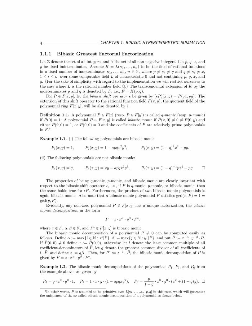
1.1.1 Bibasic Greatest Factorial Factorization
Let Z denote the set of all integers, and N the set of all non-negative integers. Let p, q, x, andy be fixed indeterminates. Assume K = L(κ1, . . . , κn) to be the field of rational functionsin a fixed number of indeterminates κ1, . . . , κn, n ∈ N, where p 6= κi 6= y and q 6= κi 6= x,1 ≤ i ≤ n, over some computable field L of characteristic 0 and not containing p, q, x, andy. (For the sake of simplicity with regard to the implementation we will restrict ourselves tothe case where L is the rational number field Q.) The transcendental extension of K by theindeterminates p and q is denoted by F , i.e., F = K(p, q).
For P ∈ F [x, y], let the bibasic shift operator ε be given by (εP )(x, y) = P (qx, py). Theextension of this shift operator to the rational function field F (x, y), the quotient field of thepolynomial ring F [x, y], will be also denoted by ε.
Definition 1.1. A polynomial P ∈ F [x] (resp. P ∈ F [y]) is called q-monic (resp. p-monic)if P (0) = 1. A polynomial P ∈ F [x, y] is called bibasic monic if P (x, 0) 6= 0 6= P (0, y) andeither P (0, 0) = 1, or P (0, 0) = 0 and the coefficients of P are relatively prime polynomialsin F .†
Example 1.1. (i) The following polynomials are bibasic monic:
P1(x, y) = 1, P2(x, y) = 1− apqx2y3, P3(x, y) = (1− q)2x2 + py.
(ii) The following polynomials are not bibasic monic:
P4(x, y) = q, P5(x, y) = xy − apqx2y3, P6(x, y) = (1− q)−1px2 + py.
The properties of being q-monic, p-monic, and bibasic monic are clearly invariant withrespect to the bibasic shift operator ε, i.e., if P is q-monic, p-monic, or bibasic monic, thenthe same holds true for εP . Furthermore, the product of two bibasic monic polynomials isagain bibasic monic. Also note that a bibasic monic polynomial P satisfies gcd(x, P ) = 1 =gcd(y, P ).
Evidently, any non-zero polynomial P ∈ F [x, y] has a unique factorization, the bibasicmonic decomposition, in the form
P = z · xα · yβ · P∗,
where z ∈ F , α, β ∈ N, and P∗ ∈ F [x, y] is bibasic monic.The bibasic monic decomposition of a polynomial P 6= 0 can be computed easily as
follows. Define α := max{i ∈ N : xi|P}, β := max{j ∈ N : yj |P}, and put P := x−α · y−β ·P .If P (0, 0) 6= 0 define z := P (0, 0), otherwise let l denote the least common multiple of allcoefficient-denominators of P , let g denote the greatest common divisor of all coefficients ofl · P , and define z := g/l. Then, for P∗ := z−1 · P , the bibasic monic decomposition of P isgiven by P = z · xα · yβ · P∗.
Example 1.2. The bibasic monic decompositions of the polynomials P4, P5, and P6 fromthe example above are given by
P4 = q · x0 · y0 · 1, P5 = 1 · x · y · (1− apqxy2), P6 =p
1− q· x0 · y0 · (x2 + (1− q)y).
†In other words, P is assumed to be primitive over L[κ1, . . . , κn, p, q] in this case, which will guaranteethe uniqueness of the so-called bibasic monic decomposition of a polynomial as shown below.
1.1. THEORETICAL BACKGROUND 5
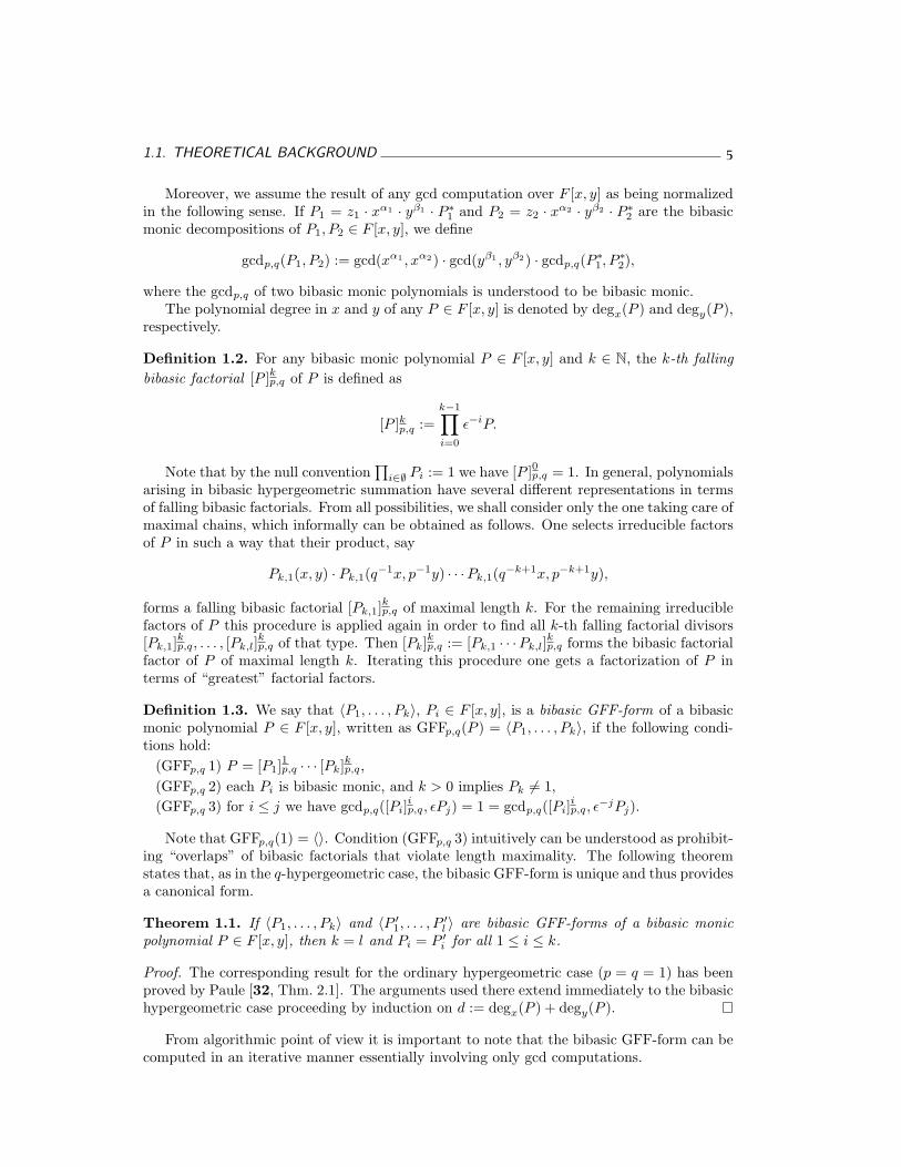
Moreover, we assume the result of any gcd computation over F [x, y] as being normalizedin the following sense. If P1 = z1 · xα1 · yβ1 · P∗1 and P2 = z2 · xα2 · yβ2 · P∗2 are the bibasicmonic decompositions of P1, P2 ∈ F [x, y], we define
gcdp,q(P1, P2) := gcd(xα1 , xα2) · gcd(yβ1 , yβ2) · gcdp,q(P∗1, P∗2),
where the gcdp,q of two bibasic monic polynomials is understood to be bibasic monic.The polynomial degree in x and y of any P ∈ F [x, y] is denoted by degx(P ) and degy(P ),
respectively.
Definition 1.2. For any bibasic monic polynomial P ∈ F [x, y] and k ∈ N, the k-th fallingbibasic factorial [P ]kp,q of P is defined as
[P ]kp,q :=k−1∏
i=0
ε−iP.
Note that by the null convention∏
i∈∅ Pi := 1 we have [P ]0p,q = 1. In general, polynomialsarising in bibasic hypergeometric summation have several different representations in termsof falling bibasic factorials. From all possibilities, we shall consider only the one taking care ofmaximal chains, which informally can be obtained as follows. One selects irreducible factorsof P in such a way that their product, say
Pk,1(x, y) · Pk,1(q−1x, p−1y) · · ·Pk,1(q−k+1x, p−k+1y),
forms a falling bibasic factorial [Pk,1]kp,q of maximal length k. For the remaining irreducible
factors of P this procedure is applied again in order to find all k-th falling factorial divisors[Pk,1]
kp,q, . . . , [Pk,l]
kp,q of that type. Then [Pk]kp,q := [Pk,1 · · ·Pk,l]
kp,q forms the bibasic factorial
factor of P of maximal length k. Iterating this procedure one gets a factorization of P interms of “greatest” factorial factors.
Definition 1.3. We say that 〈P1, . . . , Pk〉, Pi ∈ F [x, y], is a bibasic GFF-form of a bibasicmonic polynomial P ∈ F [x, y], written as GFFp,q(P ) = 〈P1, . . . , Pk〉, if the following condi-tions hold:
(GFFp,q 1) P = [P1]1p,q · · · [Pk]kp,q,
(GFFp,q 2) each Pi is bibasic monic, and k > 0 implies Pk 6= 1,(GFFp,q 3) for i ≤ j we have gcdp,q([Pi]
ip,q, εPj) = 1 = gcdp,q([Pi]
ip,q, ε−jPj).
Note that GFFp,q(1) = 〈〉. Condition (GFFp,q 3) intuitively can be understood as prohibit-ing “overlaps” of bibasic factorials that violate length maximality. The following theoremstates that, as in the q-hypergeometric case, the bibasic GFF-form is unique and thus providesa canonical form.
Theorem 1.1. If 〈P1, . . . , Pk〉 and 〈P ′1, . . . , P ′l 〉 are bibasic GFF-forms of a bibasic monicpolynomial P ∈ F [x, y], then k = l and Pi = P ′i for all 1 ≤ i ≤ k.
Proof. The corresponding result for the ordinary hypergeometric case (p = q = 1) has beenproved by Paule [32, Thm. 2.1]. The arguments used there extend immediately to the bibasichypergeometric case proceeding by induction on d := degx(P ) + degy(P ).
From algorithmic point of view it is important to note that the bibasic GFF-form can becomputed in an iterative manner essentially involving only gcd computations.
6 CHAPTER 1. BIBASIC HYPERGEOMETRIC SUMMATION
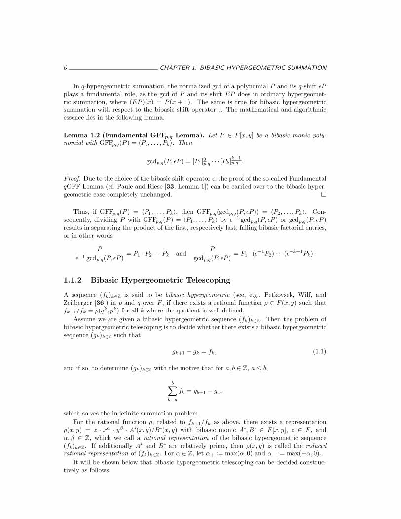
In q-hypergeometric summation, the normalized gcd of a polynomial P and its q-shift εPplays a fundamental role, as the gcd of P and its shift EP does in ordinary hypergeomet-ric summation, where (EP )(x) = P (x + 1). The same is true for bibasic hypergeometricsummation with respect to the bibasic shift operator ε. The mathematical and algorithmicessence lies in the following lemma.
Lemma 1.2 (Fundamental GFFp,q Lemma). Let P ∈ F [x, y] be a bibasic monic poly-nomial with GFFp,q(P ) = 〈P1, . . . , Pk〉. Then
gcdp,q(P, εP ) = [P1]0p,q · · · [Pk]k−1p,q .
Proof. Due to the choice of the bibasic shift operator ε, the proof of the so-called FundamentalqGFF Lemma (cf. Paule and Riese [33, Lemma 1]) can be carried over to the bibasic hyper-geometric case completely unchanged.
Thus, if GFFp,q(P ) = 〈P1, . . . , Pk〉, then GFFp,q(gcdp,q(P, εP )) = 〈P2, . . . , Pk〉. Con-sequently, dividing P with GFFp,q(P ) = 〈P1, . . . , Pk〉 by ε−1 gcdp,q(P, εP ) or gcdp,q(P, εP )results in separating the product of the first, respectively last, falling bibasic factorial entries,or in other words
P
ε−1 gcdp,q(P, εP )= P1 · P2 · · ·Pk and
P
gcdp,q(P, εP )= P1 · (ε−1P2) · · · (ε−k+1Pk).
1.1.2 Bibasic Hypergeometric Telescoping
A sequence (fk)k∈Z is said to be bibasic hypergeometric (see, e.g., Petkovsek, Wilf, andZeilberger [36]) in p and q over F , if there exists a rational function ρ ∈ F (x, y) such thatfk+1/fk = ρ(qk, pk) for all k where the quotient is well-defined.
Assume we are given a bibasic hypergeometric sequence (fk)k∈Z. Then the problem ofbibasic hypergeometric telescoping is to decide whether there exists a bibasic hypergeometricsequence (gk)k∈Z such that
gk+1 − gk = fk, (1.1)
and if so, to determine (gk)k∈Z with the motive that for a, b ∈ Z, a ≤ b,
b∑
k=a
fk = gb+1 − ga,
which solves the indefinite summation problem.For the rational function ρ, related to fk+1/fk as above, there exists a representation
ρ(x, y) = z · xα · yβ · A∗(x, y)/B∗(x, y) with bibasic monic A∗, B∗ ∈ F [x, y], z ∈ F , andα, β ∈ Z, which we call a rational representation of the bibasic hypergeometric sequence(fk)k∈Z. If additionally A∗ and B∗ are relatively prime, then ρ(x, y) is called the reducedrational representation of (fk)k∈Z. For α ∈ Z, let α+ := max(α, 0) and α− := max(−α, 0).
It will be shown below that bibasic hypergeometric telescoping can be decided construc-tively as follows.
1.1. THEORETICAL BACKGROUND 7
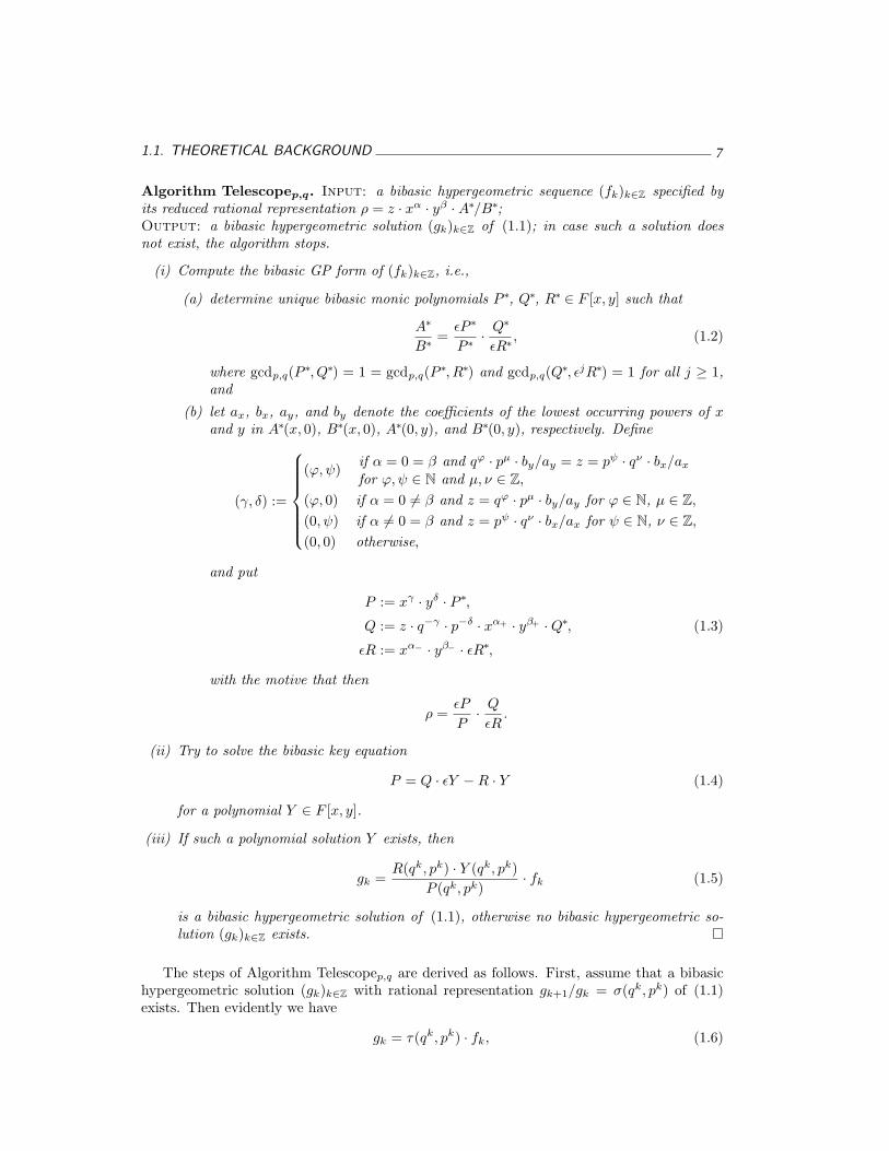
Algorithm Telescopep,q. Input: a bibasic hypergeometric sequence (fk)k∈Z specified byits reduced rational representation ρ = z · xα · yβ ·A∗/B∗;Output: a bibasic hypergeometric solution (gk)k∈Z of (1.1); in case such a solution doesnot exist, the algorithm stops.
(i) Compute the bibasic GP form of (fk)k∈Z, i.e.,
(a) determine unique bibasic monic polynomials P∗, Q∗, R∗ ∈ F [x, y] such that
A∗
B∗=
εP∗
P∗· Q∗
εR∗, (1.2)
where gcdp,q(P∗, Q∗) = 1 = gcdp,q(P∗, R∗) and gcdp,q(Q∗, εjR∗) = 1 for all j ≥ 1,and
(b) let ax, bx, ay, and by denote the coefficients of the lowest occurring powers of xand y in A∗(x, 0), B∗(x, 0), A∗(0, y), and B∗(0, y), respectively. Define
(γ, δ) :=
(ϕ,ψ) if α = 0 = β and qϕ · pµ · by/ay = z = pψ · qν · bx/ax
for ϕ,ψ ∈ N and µ, ν ∈ Z,
(ϕ, 0) if α = 0 6= β and z = qϕ · pµ · by/ay for ϕ ∈ N, µ ∈ Z,
(0, ψ) if α 6= 0 = β and z = pψ · qν · bx/ax for ψ ∈ N, ν ∈ Z,
(0, 0) otherwise,
and put
P := xγ · yδ · P∗,Q := z · q−γ · p−δ · xα+ · yβ+ ·Q∗, (1.3)
εR := xα− · yβ− · εR∗,with the motive that then
ρ =εP
P· Q
εR.
(ii) Try to solve the bibasic key equation
P = Q · εY −R · Y (1.4)
for a polynomial Y ∈ F [x, y].
(iii) If such a polynomial solution Y exists, then
gk =R(qk, pk) · Y (qk, pk)
P (qk, pk)· fk (1.5)
is a bibasic hypergeometric solution of (1.1), otherwise no bibasic hypergeometric so-lution (gk)k∈Z exists.
The steps of Algorithm Telescopep,q are derived as follows. First, assume that a bibasichypergeometric solution (gk)k∈Z with rational representation gk+1/gk = σ(qk, pk) of (1.1)exists. Then evidently we have
gk = τ(qk, pk) · fk, (1.6)
8 CHAPTER 1. BIBASIC HYPERGEOMETRIC SUMMATION
where τ(x, y) = 1/(σ(x, y)− 1) ∈ F (x, y).By relation (1.6), equation (1.1) is equivalent to
z · xα+ · yβ+ ·A∗ · ετ − xα− · yβ− ·B∗ · τ = xα− · yβ− ·B∗, (1.7)
where the reduced rational representation of (fk)k∈Z is given by ρ = z · xα · yβ ·A∗/B∗.Vice versa, any rational solution τ ∈ F (x, y) of (1.7) gives rise to a bibasic hypergeomet-
ric solution gk := τ(qk, pk) · fk of (1.1). This means, bibasic hypergeometric telescoping isequivalent to finding a rational solution τ of (1.7).
Any τ ∈ F (x, y) can be represented as the quotient of relatively prime polynomials in theform τ = U/V where U ,V ∈ F [x, y] with V = xϕ · yψ · V∗ the bibasic monic decompositionof V. In case such a solution τ of (1.7) exists, assume we know V or a multiple V ∈ F [x, y]of V. Then by clearing denominators in
z · xα+ · yβ+ ·A∗ · εU
εV− xα− · yβ− ·B∗ · U
V= xα− · yβ− ·B∗,
the problem reduces further to finding a polynomial solution U ∈ F [x, y] of the resultingdifference equation with polynomial coefficients,
z · xα+ · yβ+ ·A∗ · V · εU − xα− · yβ− ·B∗ · (εV ) · U = xα− · yβ− ·B∗ · V · εV. (1.8)
Note that at least one polynomial solution, namely U = U · V/V, exists. Furthermore,equations of that type simplify by canceling gcdp,q’s. For instance, in order to get moreinformation about the denominator V, let Vi := εiV/ gcdp,q(V, εV), i ∈ {0, 1}. Then (1.7) isequivalent to
z · xα+ · yβ+ ·A∗ · V0 · εU − xα− · yβ− ·B∗ · V1 · U = xα− · yβ− ·B∗ · V0 · V1 · gcdp,q(V, εV).(1.9)
Now, if 〈P1, . . . ,Pm〉, m ∈ N, is the bibasic GFF-form of V∗, it follows from gcdp,q(U ,V) =1 = gcdp,q(V0,V1) and the Fundamental GFFp,q Lemma that
V0 = (ε0P1) · · · (ε−m+1Pm) | B∗ and V1 = qϕ · pψ · (εP1) · · · (εPm) | A∗.
This observation gives rise to a simple and straightforward algorithm for computing amultiple V ∗ := [P1]
1p,q · · · [Pn]np,q of V∗. For instance, if P1 := gcdp,q(ε−1A∗, B∗) then obviously
P1|P1. Actually, one can iteratively extract bibasic monic Pi-multiples Pi such that εPi|A∗and ε−i+1Pi|B∗ by the following algorithm.
Algorithm V∗MULT. Input: relatively prime and bibasic monic polynomials A∗, B∗ ∈F [x, y] that constitute the bibasic monic quotient of ρ = z · xα · yβ ·A∗/B∗ ∈ F (x, y);Output: bibasic monic polynomials P1, . . . , Pn such that V ∗ := [P1]
1p,q · · · [Pn]np,q is a multiple
of V∗, the bibasic monic part of the denominator V = xϕ · yψ · V∗ of τ ∈ F (x, y).
(i) Compute n = min{j ∈ N | gcdp,q(ε−1A∗, εk−1B∗) = 1 for all integers k > j}.(ii) Set A0 = A∗, B0 = B∗, and compute for i from 1 to n:
Pi = gcdp,q(ε−1Ai−1, εi−1Bi−1),
Ai = Ai−1/εPi,
Bi = Bi−1/ε−i+1Pi.
1.1. THEORETICAL BACKGROUND 9
A proof for the fact that the Pi are indeed multiples of the Pi has been worked out for theordinary hypergeometric case by Paule [32, Lemma 5.1]. It can be carried over to the bibasichypergeometric world almost word by word. Hence we leave the steps of the verification tothe reader.
Note that in general step (i) of Algorithm V∗MULT would be a rather time-consuming taskinvolving resultant computations which could be solved by generalizing the univariate case(cf. Abramov, Paule, and Petkovsek [1]) in a straightforward way, for instance, as follows.Define R1(v, w) := Resx(A∗(x, y), B∗(vx, wy)) and R2(v, w) := Resy(A∗(x, y), B∗(vx, wy)),viewed as polynomials of v and w over F [y], respectively F [x]. Then n is the maximalpositive integer such that R1(qn, pn) · R2(qn, pn) = 0 if such an integer exists, and n = 0otherwise. However, in our implementation we make use of the fact that A∗ and B∗ alreadycome in nicely factored form so that the computation of n boils down to a comparison ofthose factors.
Moreover, Algorithm V∗MULT also delivers the constituents of the bibasic monic part ofthe GP representation (1.2) as stated in the following lemma.
Lemma 1.3. Let n, An, Bn, and the tuple 〈P1, . . . , Pn〉 be computed as in AlgorithmV∗MULT. Then for P∗ = V ∗, Q∗ = An, and R∗ = ε−1Bn we have
A∗
B∗=
εP∗
P∗· Q∗
εR∗,
where gcdp,q(P∗, Q∗) = 1 = gcdp,q(P∗, R∗) and gcdp,q(Q∗, εjR∗) = 1 for all j ≥ 1.
For more details on GP representations in the q-hypergeometric case, see Abramov, Paule,and Petkovsek [1], or Paule and Strehl [34]. The results obtained there also apply to thebibasic hypergeometric case, in particular we have the following.
Lemma 1.4. The polynomials P∗, Q∗, and R∗ of the bibasic monic part of the GP represen-tation (1.2) are unique.
Proof. The corresponding result for the case p = q = 1 has been proved by Petkovsek [35].The argumentation extends directly to the q- and bibasic hypergeometric case.
With the multiple V ∗ of V∗ in hands, all what is left for solving (1.7), and thus the bibasichypergeometric telescoping problem (1.1), is to determine appropriate multiplicities γ and δsuch that
V = xγ · yδ · V ∗ is a multiple of V = xϕ · yψ · V∗.
For that we consider equation (1.9) again in the equivalent version
z · xα+ · yβ+ ·A∗ · V∗ · εU − xα− · yβ− ·B∗ · qϕ · pψ · (εV∗) · U = xα− · yβ− ·B∗ · V∗ · εV,(1.10)
and distinguish the following cases corresponding to step (ib) of Algorithm Telescopep,q.
(i) Assume that either α− 6= 0 or α+ 6= 0. In the first case we have α+ = 0 and xα− | U ,hence ϕ must be 0 because of gcdp,q(U ,V) = 1. This means, we can choose γ := 0. Inthe second case we have α− = 0 and xmin(α+,ϕ) | U , because of εV = xϕ ·yψ ·qϕ ·pψ ·εV∗.Again ϕ must be 0, and again we can choose γ := 0. Analogously, if β 6= 0 we canchoose δ := 0.
10 CHAPTER 1. BIBASIC HYPERGEOMETRIC SUMMATION
(ii) Assume that α = 0 and β 6= 0, hence ψ = 0 by (i). For ϕ > 0, evaluating equation (1.10)at x = 0 results in
z · yβ+ ·A∗(0, y) · V∗(0, y) · U(0, py)− yβ− ·B∗(0, y) · qϕ · V∗(0, py) · U(0, y) = 0.(1.11)
In order to evaluate (1.11) at y = 0, note that P ∈ F [x, y] being bibasic monic doesnot necessarily imply that P (0, y) ∈ F [y] is p-monic. To overcome this problem, let usconsider the p-monic decompositions of U(0, y) and V∗(0, y), say U(0, y) = u ·yβu · U(y)and V∗(0, y) = v · yβv · V (y), respectively. Now, dividing equation (1.11) by U(0, y) ·V∗(0, y) 6= 0 leads to
z · yβ+ ·A∗(0, y) · pβu · U(py)U(y)
− yβ− ·B∗(0, y) · qϕ · pβv · V (py)V (y)
= 0. (1.12)
Additionally, let the p-monic decompositions of A∗(0, y) and B∗(0, y) be given byA∗(0, y) = ay · yβa · A(y) and B∗(0, y) = by · yβb · B(y), respectively. Then the powersyβa+β+ and yβb+β− must be equal, and after cancellation eq. (1.12) at y = 0 turns into
z · ay · pβu − by · qϕ · pβv = 0.
This means, we obtain as a condition for ϕ > 0 that z = qϕ · pµ · by/ay with µ ∈ Z.Hence, in this case we choose γ := ϕ, i.e., we set γ to this q-power if z has this particularform, and γ := 0 otherwise. Analogously, if α 6= 0 and β = 0 we define δ := ψ > 0, ifz = pψ · qν · bx/ax with ν ∈ Z, and δ := 0 otherwise.
(iii) Finally, for the case α = 0 = β similar reasoning as in case (ii) leads to the conditions
qϕ · pµ · by/ay = z = pψ · qν · bx/ax, (1.13)
for ϕ > 0 or ψ > 0, and µ, ν ∈ Z. Thus, if both conditions (1.13) are satisfied we chooseγ := ϕ and δ := ψ, and otherwise γ = δ := 0.
The remaining steps of Algorithm Telescopep,q now are explained as follows. Once again,employing the GP representation for the bibasic monic quotient of ρ,
A∗
B∗=
εP∗
P∗· Q∗
εR∗,
it is easily seen that equation (1.8) can be written as
z · q−γ · p−δ · xα+ · yβ+ · Q∗
εR∗· εU − xα− · yβ− · U = xγ+α− · yδ+β− · P∗. (1.14)
Because of relative primeness of certain polynomials, we observe that xα− |U , yβ− |U , andεR∗ | εU . Hence by defining Y by the relation
U = xα− · yβ− · q−α− · p−β− ·R∗ · Y,
the task to solve equation (1.8) for U reduces to solve
z · q−γ · p−δ · xα+ · yβ+ ·Q∗ · εY − xα− · yβ− · q−α− · p−β− ·R∗ · Y = xγ · yδ · P∗ (1.15)
for Y ∈ F [x, y]. By definition (1.3) of P , Q, and R, equation (1.15) immediately turns intothe bibasic key equation (1.4),
Q · εY −R · Y = P.
1.2. DEGREE SETTING FOR SOLVING THE BIBASIC KEY EQUATION 11
Finally, from U/V = R · Y/P , again by definition (1.3), it follows directly that
gk =R(qk, pk) · Y (qk, pk)
P (qk, pk)· fk
as in (1.5) actually is a solution of the bibasic hypergeometric telescoping problem (1.1).This completes the proof of the correctness of Algorithm Telescopep,q.
1.2 Degree Setting for Solving the Bibasic Key Equation
To solve the bibasic key equation
P = Q · εY −R · Y (1.16)
we first have to determine degree bounds d1 and d2, say, for the solution polynomial Y ∈F [x, y] with respect to x and y, respectively, as shown in Theorem 1.5 below. Then we put
Y (x, y) :=d1∑
i=0
d2∑
j=0
yi,j · xi · yj
with undetermined yi,j and solve (1.16) for the yi,j by equating to zero all coefficients of xiyj
in the equation
P −Q · εY + R · Y = 0,
which corresponds to solving a system of linear equations.
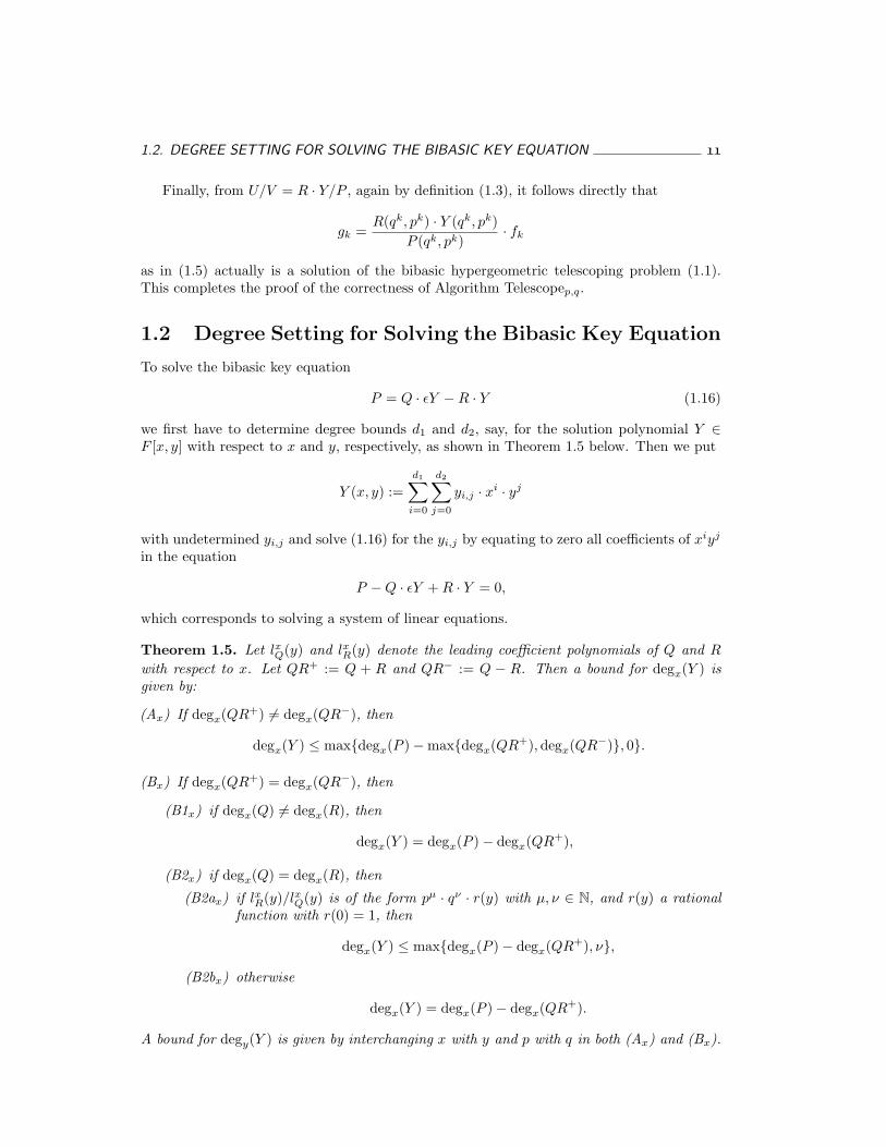
Theorem 1.5. Let lxQ(y) and lxR(y) denote the leading coefficient polynomials of Q and R
with respect to x. Let QR+ := Q + R and QR− := Q − R. Then a bound for degx(Y ) isgiven by:
(Ax) If degx(QR+) 6= degx(QR−), then
degx(Y ) ≤ max{degx(P )−max{degx(QR+), degx(QR−)}, 0}.
(Bx) If degx(QR+) = degx(QR−), then
(B1x) if degx(Q) 6= degx(R), then
degx(Y ) = degx(P )− degx(QR+),
(B2x) if degx(Q) = degx(R), then
(B2ax) if lxR(y)/lxQ(y) is of the form pµ · qν · r(y) with µ, ν ∈ N, and r(y) a rationalfunction with r(0) = 1, then
degx(Y ) ≤ max{degx(P )− degx(QR+), ν},
(B2bx) otherwise
degx(Y ) = degx(P )− degx(QR+).
A bound for degy(Y ) is given by interchanging x with y and p with q in both (Ax) and (Bx).
12 CHAPTER 1. BIBASIC HYPERGEOMETRIC SUMMATION
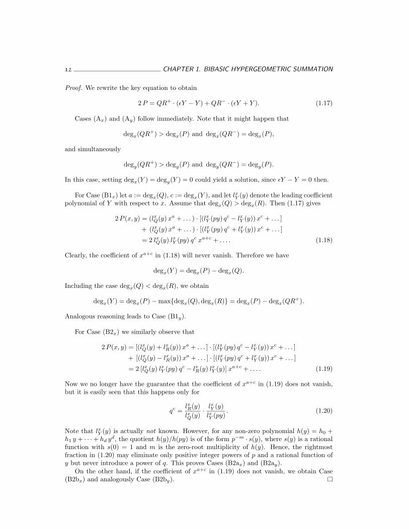
Proof. We rewrite the key equation to obtain
2 P = QR+ · (εY − Y ) + QR− · (εY + Y ). (1.17)
Cases (Ax) and (Ay) follow immediately. Note that it might happen that
degx(QR+) > degx(P ) and degx(QR−) = degx(P ),
and simultaneously
degy(QR+) > degy(P ) and degy(QR−) = degy(P ).
In this case, setting degx(Y ) = degy(Y ) = 0 could yield a solution, since εY − Y = 0 then.
For Case (B1x) let a := degx(Q), c := degx(Y ), and let lxY (y) denote the leading coefficientpolynomial of Y with respect to x. Assume that degx(Q) > degx(R). Then (1.17) gives
2 P (x, y) = (lxQ(y)xa + . . . ) · [(lxY (py) qc − lxY (y)) xc + . . . ]
+ (lxQ(y)xa + . . . ) · [(lxY (py) qc + lxY (y)) xc + . . . ]
= 2 lxQ(y) lxY (py) qc xa+c + . . . . (1.18)
Clearly, the coefficient of xa+c in (1.18) will never vanish. Therefore we have
degx(Y ) = degx(P )− degx(Q).
Including the case degx(Q) < degx(R), we obtain
degx(Y ) = degx(P )−max{degx(Q), degx(R)} = degx(P )− degx(QR+).
Analogous reasoning leads to Case (B1y).
For Case (B2x) we similarly observe that
2 P (x, y) = [(lxQ(y) + lxR(y)) xa + . . . ] · [(lxY (py) qc − lxY (y)) xc + . . . ]
+ [(lxQ(y)− lxR(y)) xa + . . . ] · [(lxY (py) qc + lxY (y)) xc + . . . ]
= 2 [lxQ(y) lxY (py) qc − lxR(y) lxY (y)] xa+c + . . . . (1.19)
Now we no longer have the guarantee that the coefficient of xa+c in (1.19) does not vanish,but it is easily seen that this happens only for
qc =lxR(y)lxQ(y)
· lxY (y)lxY (py)
. (1.20)
Note that lxY (y) is actually not known. However, for any non-zero polynomial h(y) = h0 +h1 y + · · ·+ hd yd, the quotient h(y)/h(py) is of the form p−m · s(y), where s(y) is a rationalfunction with s(0) = 1 and m is the zero-root multiplicity of h(y). Hence, the rightmostfraction in (1.20) may eliminate only positive integer powers of p and a rational function ofy but never introduce a power of q. This proves Cases (B2ax) and (B2ay).
On the other hand, if the coefficient of xa+c in (1.19) does not vanish, we obtain Case(B2bx) and analogously Case (B2by).
1.3. APPLICATIONS 13
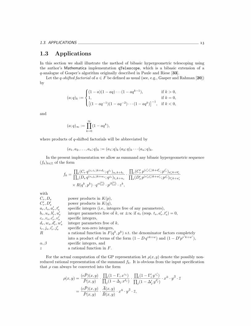
1.3 Applications
In this section we shall illustrate the method of bibasic hypergeometric telescoping usingthe author’s Mathematica implementation qTelescope, which is a bibasic extension of aq-analogue of Gosper’s algorithm originally described in Paule and Riese [33].
Let the q-shifted factorial of a ∈ F be defined as usual (see, e.g., Gasper and Rahman [20])by
(a; q)k :=
(1− a)(1− aq) · · · (1− aqk−1), if k > 0,1, if k = 0,[(1− aq−1)(1− aq−2) · · · (1− aqk)
]−1, if k < 0,
and
(a; q)∞ :=∞∏
k=0
(1− aqk),
where products of q-shifted factorials will be abbreviated by
(a1, a2, . . . , an; q)k := (a1; q)k (a2; q)k · · · (an; q)k.
In the present implementation we allow as summand any bibasic hypergeometric sequence(fk)k∈Z of the form
fk =∏
r(Cr q(crir)k+dr ; qir )ark+br∏s(Ds q(vsjs)k+ws ; qjs)tsk+us
·∏
r(C′r p(c′ri′r)k+d′r ; pi′r )a′rk+b′r∏
s(D′s p(v′sj′s)k+w′s ; pj′s)t′sk+u′s
×R(qk, pk) · qα(k2) · pβ(k
2) · zk,
withCr, Ds power products in K(p),C ′r, D
′s power products in K(q),
ar, ts, a′r, t
′s specific integers (i.e., integers free of any parameters),
br, us, b′r, u
′s integer parameters free of k, or ±∞ if ar (resp. ts, a
′r, t
′s) = 0,
cr, vs, c′r, v
′s specific integers,
dr, ws, d′r, w
′s integer parameters free of k,
ir, js, i′r, j
′s specific non-zero integers,
R a rational function in F (qk, pk) s.t. the denominator factors completelyinto a product of terms of the form (1−D qvk+w) and (1−D′pv′k+w′),
α, β specific integers, andz a rational function in F .
For the actual computation of the GP representation let ρ(x, y) denote the possibly non-reduced rational representation of the summand fk. It is obvious from the input specificationthat ρ can always be converted into the form
ρ(x, y) =(εP )(x, y)P (x, y)
·∏
i(1− Γi xγi)∏j(1−∆j xδj )
·∏
i(1− Γ′i yγ′i)∏j(1−∆′
j yδ′j )· xα · yβ · z
=(εP )(x, y)P (x, y)
· A(x, y)B(x, y)
· xα · yβ · z,
14 CHAPTER 1. BIBASIC HYPERGEOMETRIC SUMMATION
where P is bibasic monic and satisfies gcdp,q(P , A) = 1 = gcdp,q(εP , B); the Γi, ∆j , Γ′i, ∆′j
are power products in F , the γi, δj , γ′i, δ
′j are positive integers, α, β ∈ Z, and z ∈ F .
Concerning Algorithm V∗MULT, it is clear from above that any P 6= 1 will actuallycontribute to [P1]
1p,q and thus can be treated separately. Due to our input restrictions — this
is the reason for admitting only power products instead of arbitrary rational functions — itis possible to find n in step (i) of Algorithm V∗MULT simply by comparing all factors in Aand B as already mentioned.
Furthermore, since A and B are both products of a q-monic and a p-monic polynomial,they will never contribute to bx/ax and by/ay. Thus, bx/ax and by/ay are in any case integerpowers of q and p, respectively, coming from εP /P . Therefore, they do not take influence onthe computation of γ and δ at all.
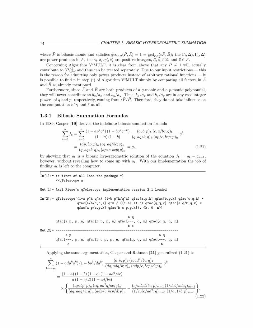
1.3.1 Bibasic Summation Formulas
In 1989, Gasper [19] derived the indefinite bibasic summation formulan∑
k=0
fk =n∑
k=0
(1− apkqk) (1− bpkq−k)(1− a) (1− b)
(a, b; p)k (c, a/bc; q)k
(q, aq/b; q)k (ap/c, bcp; p)kqk
=(ap, bp; p)n (cq, aq/bc; q)n
(q, aq/b; q)n (ap/c, bcp; p)n= gn (1.21)
by showing that gk is a bibasic hypergeometric solution of the equation fk = gk − gk−1,however, without revealing how to come up with gk. With our implementation the job offinding gk is left to the computer.
In[1]:= (* first of all load the package *)
<<qTelescope.m
Out[1]= Axel Riese’s qTelescope implementation version 2.1 loaded
In[2]:= qTelescope[(1-a p^k q^k) (1-b p^k/q^k) qfac[a,p,k] qfac[b,p,k] qfac[c,q,k] *
qfac[a/b/c,q,k] q^k / ((1-a) (1-b) qfac[q,q,k] qfac[a q/b,q,k] *
qfac[a p/c,p,k] qfac[b c p,p,k]), {k, 0, n}]
a q
qfac[a p, p, n] qfac[b p, p, n] qfac[---, q, n] qfac[c q, q, n]
b c
Out[2]= ---------------------------------------------------------------
a p a q
qfac[---, p, n] qfac[b c p, p, n] qfac[q, q, n] qfac[---, q, n]
c b
Applying the same argumentation, Gasper and Rahman [21] generalized (1.21) ton∑
k=−m
(1− adpkqk) (1− bpk/dqk)(a, b; p)k (c, ad2/bc; q)k
(dq, adq/b; q)k (adp/c, bcp/d; p)kqk
=(1− a) (1− b) (1− c) (1− ad2/bc)
d (1− c/d) (1− ad/bc)
×{
(ap, bp; p)n (cq, ad2q/bc; q)n
(dq, adq/b; q)n (adp/c, bcp/d; p)n− (c/ad, d/bc; p)m+1 (1/d, b/ad; q)m+1
(1/c, bc/ad2; q)m+1 (1/a, 1/b; p)m+1
}.
(1.22)
1.3. APPLICATIONS 15
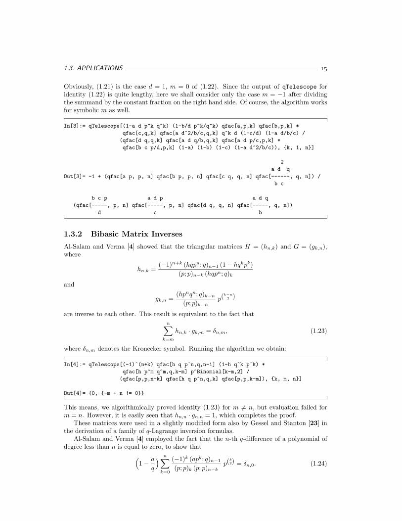
Obviously, (1.21) is the case d = 1, m = 0 of (1.22). Since the output of qTelescope foridentity (1.22) is quite lengthy, here we shall consider only the case m = −1 after dividingthe summand by the constant fraction on the right hand side. Of course, the algorithm worksfor symbolic m as well.
In[3]:= qTelescope[(1-a d p^k q^k) (1-b/d p^k/q^k) qfac[a,p,k] qfac[b,p,k] *
qfac[c,q,k] qfac[a d^2/b/c,q,k] q^k d (1-c/d) (1-a d/b/c) /
(qfac[d q,q,k] qfac[a d q/b,q,k] qfac[a d p/c,p,k] *
qfac[b c p/d,p,k] (1-a) (1-b) (1-c) (1-a d^2/b/c)), {k, 1, n}]
2
a d q
Out[3]= -1 + (qfac[a p, p, n] qfac[b p, p, n] qfac[c q, q, n] qfac[------, q, n]) /
b c
b c p a d p a d q
(qfac[-----, p, n] qfac[-----, p, n] qfac[d q, q, n] qfac[-----, q, n])
d c b
1.3.2 Bibasic Matrix Inverses
Al-Salam and Verma [4] showed that the triangular matrices H = (hn,k) and G = (gk,n),where
hn,k =(−1)n+k (hqpn; q)n−1 (1− hqkpk)
(p; p)n−k (hqpn; q)k
and
gk,n =(hpnqn; q)k−n
(p; p)k−np(k−n
2 )
are inverse to each other. This result is equivalent to the fact thatn∑
k=m
hn,k · gk,m = δn,m, (1.23)
where δn,m denotes the Kronecker symbol. Running the algorithm we obtain:
In[4]:= qTelescope[(-1)^(n+k) qfac[h q p^n,q,n-1] (1-h q^k p^k) *
qfac[h p^m q^m,q,k-m] p^Binomial[k-m,2] /
(qfac[p,p,n-k] qfac[h q p^n,q,k] qfac[p,p,k-m]), {k, m, n}]
Out[4]= {0, {-m + n != 0}}
This means, we algorithmically proved identity (1.23) for m 6= n, but evaluation failed form = n. However, it is easily seen that hn,n · gn,n = 1, which completes the proof.
These matrices were used in a slightly modified form also by Gessel and Stanton [23] inthe derivation of a family of q-Lagrange inversion formulas.
Al-Salam and Verma [4] employed the fact that the n-th q-difference of a polynomial ofdegree less than n is equal to zero, to show that
(1− a
q
) n∑
k=0
(−1)k (apk; q)n−1
(p; p)k (p; p)n−kp(k
2) = δn,0. (1.24)
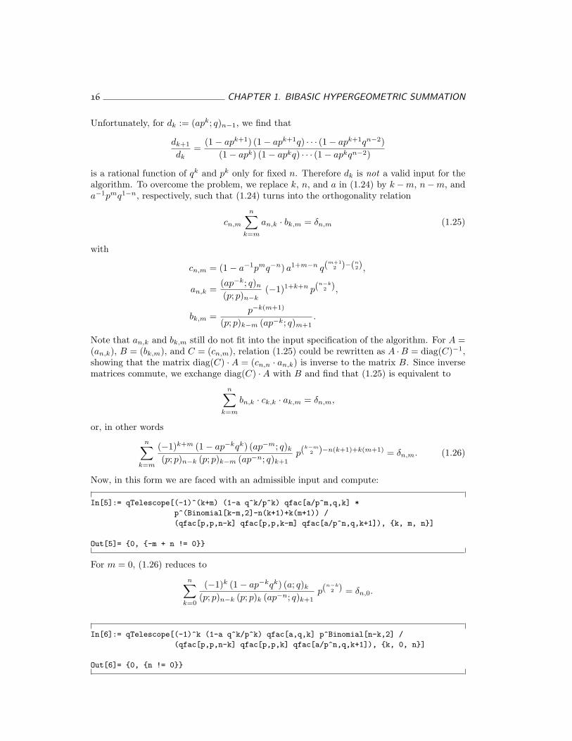
16 CHAPTER 1. BIBASIC HYPERGEOMETRIC SUMMATION
Unfortunately, for dk := (apk; q)n−1, we find that
dk+1
dk=
(1− apk+1) (1− apk+1q) · · · (1− apk+1qn−2)(1− apk) (1− apkq) · · · (1− apkqn−2)
is a rational function of qk and pk only for fixed n. Therefore dk is not a valid input for thealgorithm. To overcome the problem, we replace k, n, and a in (1.24) by k −m, n−m, anda−1pmq1−n, respectively, such that (1.24) turns into the orthogonality relation
cn,m
n∑
k=m
an,k · bk,m = δn,m (1.25)
with
cn,m = (1− a−1pmq−n) a1+m−n q(m+1
2 )−(n2),
an,k =(ap−k; q)n
(p; p)n−k(−1)1+k+n p(n−k
2 ),
bk,m =p−k(m+1)
(p; p)k−m (ap−k; q)m+1.
Note that an,k and bk,m still do not fit into the input specification of the algorithm. For A =(an,k), B = (bk,m), and C = (cn,m), relation (1.25) could be rewritten as A ·B = diag(C)−1,showing that the matrix diag(C) · A = (cn,n · an,k) is inverse to the matrix B. Since inversematrices commute, we exchange diag(C) ·A with B and find that (1.25) is equivalent to
n∑
k=m
bn,k · ck,k · ak,m = δn,m,
or, in other wordsn∑
k=m
(−1)k+m (1− ap−kqk) (ap−m; q)k
(p; p)n−k (p; p)k−m (ap−n; q)k+1p(k−m
2 )−n(k+1)+k(m+1) = δn,m. (1.26)
Now, in this form we are faced with an admissible input and compute:
In[5]:= qTelescope[(-1)^(k+m) (1-a q^k/p^k) qfac[a/p^m,q,k] *
p^(Binomial[k-m,2]-n(k+1)+k(m+1)) /
(qfac[p,p,n-k] qfac[p,p,k-m] qfac[a/p^n,q,k+1]), {k, m, n}]
Out[5]= {0, {-m + n != 0}}
For m = 0, (1.26) reduces to
n∑
k=0
(−1)k (1− ap−kqk) (a; q)k
(p; p)n−k (p; p)k (ap−n; q)k+1p(n−k
2 ) = δn,0.
In[6]:= qTelescope[(-1)^k (1-a q^k/p^k) qfac[a,q,k] p^Binomial[n-k,2] /
(qfac[p,p,n-k] qfac[p,p,k] qfac[a/p^n,q,k+1]), {k, 0, n}]
Out[6]= {0, {n != 0}}
1.3. APPLICATIONS 17
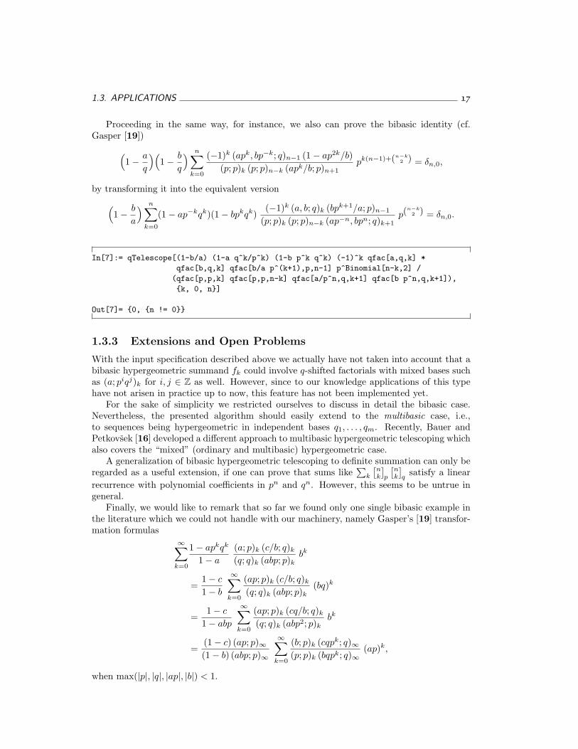
Proceeding in the same way, for instance, we also can prove the bibasic identity (cf.Gasper [19])
(1− a
q
)(1− b
q
) n∑
k=0
(−1)k (apk, bp−k; q)n−1 (1− ap2k/b)(p; p)k (p; p)n−k (apk/b; p)n+1
pk(n−1)+(n−k2 ) = δn,0,
by transforming it into the equivalent version
(1− b
a
) n∑
k=0
(1− ap−kqk)(1− bpkqk)(−1)k (a, b; q)k (bpk+1/a; p)n−1
(p; p)k (p; p)n−k (ap−n, bpn; q)k+1p(n−k
2 ) = δn,0.
In[7]:= qTelescope[(1-b/a) (1-a q^k/p^k) (1-b p^k q^k) (-1)^k qfac[a,q,k] *
qfac[b,q,k] qfac[b/a p^(k+1),p,n-1] p^Binomial[n-k,2] /
(qfac[p,p,k] qfac[p,p,n-k] qfac[a/p^n,q,k+1] qfac[b p^n,q,k+1]),
{k, 0, n}]
Out[7]= {0, {n != 0}}
1.3.3 Extensions and Open Problems
With the input specification described above we actually have not taken into account that abibasic hypergeometric summand fk could involve q-shifted factorials with mixed bases suchas (a; piqj)k for i, j ∈ Z as well. However, since to our knowledge applications of this typehave not arisen in practice up to now, this feature has not been implemented yet.
For the sake of simplicity we restricted ourselves to discuss in detail the bibasic case.Nevertheless, the presented algorithm should easily extend to the multibasic case, i.e.,to sequences being hypergeometric in independent bases q1, . . . , qm. Recently, Bauer andPetkovsek [16] developed a different approach to multibasic hypergeometric telescoping whichalso covers the “mixed” (ordinary and multibasic) hypergeometric case.
A generalization of bibasic hypergeometric telescoping to definite summation can only beregarded as a useful extension, if one can prove that sums like
∑k
[nk
]p
[nk
]q
satisfy a linearrecurrence with polynomial coefficients in pn and qn. However, this seems to be untrue ingeneral.
Finally, we would like to remark that so far we found only one single bibasic example inthe literature which we could not handle with our machinery, namely Gasper’s [19] transfor-mation formulas
∞∑
k=0
1− apkqk
1− a
(a; p)k (c/b; q)k
(q; q)k (abp; p)kbk
=1− c
1− b
∞∑
k=0
(ap; p)k (c/b; q)k
(q; q)k (abp; p)k(bq)k
=1− c
1− abp
∞∑
k=0
(ap; p)k (cq/b; q)k
(q; q)k (abp2; p)kbk
=(1− c) (ap; p)∞(1− b) (abp; p)∞
∞∑
k=0
(b; p)k (cqpk; q)∞(p; p)k (bqpk; q)∞
(ap)k,
when max(|p|, |q|, |ap|, |b|) < 1.

18
19
Chapter 2
Automatic Generation ofq-Identities
Using the author’s Mathematica implementation qZeil of a q-analogue of Zeilberger’s algo-rithm (cf. Paule and Riese [33]) for definite q-hypergeometric summation we will show inthis chapter how the concept of WZ-pairs introduced by Wilf and Zeilberger [44] generalizesto the q-case giving new identities from existing ones “for free”, i.e., without too much addi-tional effort. In particular, we shall focus our attention on generating companion and dualidentities from qWZ-pairs. Similar to Gessel’s [22] systematic investigation of dual identityproduction for the q = 1 case, we shall apply this method to several “standard” terminatingq-identities leading to a large number of new identities as well as identities appearing in thecontext of Bailey chains (see, e.g., Andrews [10], Paule [30], or Chapter 3).
2.1 q-Hypergeometric Telescoping and qWZ-Certifica-tion
Analogous to Zeilberger’s [46] algorithm its q-analogue takes terminating q-hypergeometricsums as input. The output is a linear recurrence that is satisfied by the input sum, togetherwith a rational function which serves as the proof certificate. It is important to note thatthe proof certificate enables an independent verification of the output recurrence merely bychecking a rational function identity. This means, the algorithm itself supplies completeinformation for a correctness check which works independently of the steps in which theoutput recurrence was manufactured.
The backbone of the author’s q-Zeilberger implementation is Algorithm qTelescope, aq-analogue of Gosper’s [24] algorithm for indefinite hypergeometric summation based on aq-version of Paule’s [32] concept of greatest factorial factorization. A detailed description ofAlgorithm qTelescope is given in Paule and Riese [33].
Let Z denote the set of all integers, N the set of all non-negative integers, and N+ := N\{0}the set of all positive integers. Assume K = L(κ1, . . . , κm) to be the field of rational functionsin a fixed number of indeterminates κ1, . . . , κm, all different from q, over some computablefield L of characteristic 0. (For the sake of simplicity with regard to the implementation wewill restrict ourselves to the case where L is the rational number field Q.) The transcendentalextension of K by the indeterminate q is denoted by F , i.e., F = K(q).
A sequence (fk) with values in F , where k runs through all integers, is said to be
20 CHAPTER 2. AUTOMATIC GENERATION OF q-IDENTITIES
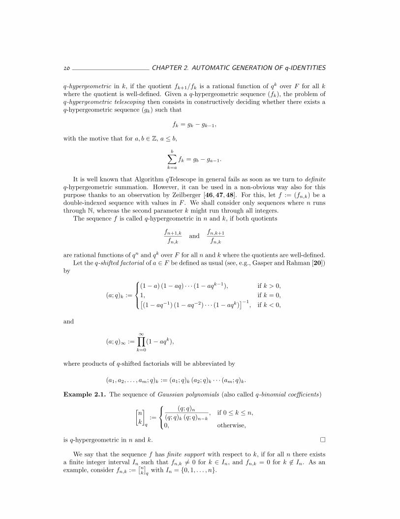
q-hypergeometric in k, if the quotient fk+1/fk is a rational function of qk over F for all kwhere the quotient is well-defined. Given a q-hypergeometric sequence (fk), the problem ofq-hypergeometric telescoping then consists in constructively deciding whether there exists aq-hypergeometric sequence (gk) such that
fk = gk − gk−1,
with the motive that for a, b ∈ Z, a ≤ b,
b∑
k=a
fk = gb − ga−1.
It is well known that Algorithm qTelescope in general fails as soon as we turn to definiteq-hypergeometric summation. However, it can be used in a non-obvious way also for thispurpose thanks to an observation by Zeilberger [46,47,48]. For this, let f := (fn,k) be adouble-indexed sequence with values in F . We shall consider only sequences where n runsthrough N, whereas the second parameter k might run through all integers.
The sequence f is called q-hypergeometric in n and k, if both quotients
fn+1,k
fn,kand
fn,k+1
fn,k
are rational functions of qn and qk over F for all n and k where the quotients are well-defined.Let the q-shifted factorial of a ∈ F be defined as usual (see, e.g., Gasper and Rahman [20])
by
(a; q)k :=
(1− a) (1− aq) · · · (1− aqk−1), if k > 0,1, if k = 0,[(1− aq−1) (1− aq−2) · · · (1− aqk)
]−1, if k < 0,
and
(a; q)∞ :=∞∏
k=0
(1− aqk),
where products of q-shifted factorials will be abbreviated by
(a1, a2, . . . , am; q)k := (a1; q)k (a2; q)k · · · (am; q)k.
Example 2.1. The sequence of Gaussian polynomials (also called q-binomial coefficients)
[n
k
]
q
:=
(q; q)n
(q; q)k (q; q)n−k, if 0 ≤ k ≤ n,
0, otherwise,
is q-hypergeometric in n and k.
We say that the sequence f has finite support with respect to k, if for all n there existsa finite integer interval In such that fn,k 6= 0 for k ∈ In, and fn,k = 0 for k 6∈ In. As anexample, consider fn,k :=
[nk
]q
with In = {0, 1, . . . , n}.
2.1. q-HYPERGEOMETRIC TELESCOPING AND qWZ-CERTIFICATION 21
Given f being q-hypergeometric in n and k, one can prove under mild side-conditions, asdemonstrated in Wilf and Zeilberger [45], that for a certain integer d ≥ 0 and n ≥ d thereexists a linear recurrence
σ0(n) fn,k + σ1(n) fn−1,k + · · ·+ σd(n) fn−d,k = gn,k − gn,k−1, (2.1)
where the coefficients are polynomials in qn not depending on k and not all zero, and wheregn,k is a rational function multiple of fn,k and thus q-hypergeometric in n and k, too. Giventhe order d, which in general is not known a priori, gn,k and also the coefficient polynomialsσi(n) are determined by q-hypergeometric telescoping, i.e., by Algorithm qTelescope.
Assume that f has finite support with respect to k. Then summing both sides of (2.1)over all k results in
σ0(n)Sn + σ1(n) Sn−1 + · · ·+ σd(n) Sn−d = 0, (2.2)
a recurrence for the sum sequence Sn :=∑
k fn,k, a finite sum due to the finite supportproperty. We use the convention that the summation parameter k runs through all theintegers, in case the summation range is not specified explicitly.
Now the qWZ-certificate (for short: certificate) of recurrence (2.1) or (2.2), respectively,by definition is the rational function cert(n, k), rational in qn and qk, such that
gn,k = cert(n, k) · fn,k.
Evidently, with the certificate in hands the verification of (2.1), and therefore (2.2),reduces to checking the rational function identity
r(n, k) = cert(n, k)− cert(n, k − 1) · fn,k−1
fn,k,
where r(n, k), rational in qn and qk, comes from rewriting the left hand side of (2.1) asr(n, k) · fn,k. The computation of r(n, k) is straightforward, because any fn−i,k can bewritten as a rational function multiple of fn,k, for instance, fn−1,k = (fn−1,k/fn,k) · fn,k.
In the inhomogeneous case, i.e., if f does not have finite support, or, if one is interestedin summation with bounds not naturally induced by the finite support, we have to introducethe corresponding correction terms in (2.2). For more details, see Paule and Riese [33].
It is well known that Zeilberger’s algorithm and especially its q-analogue do not alwaysdeliver the recurrence with minimal order. However, several approaches have been devel-oped to decrease the order to the expected one, such as Paule’s [31] method of creativesymmetrizing (see also Paule and Riese [33], or Petkovsek, Wilf, and Zeilberger [36]).
Finally, suppose that we want to prove a closed form summation identity∑
kan,k = bn,
where (an,k) has finite support and bn 6= 0 for all n. By putting fn,k := an,k/bn, the identityto be proved may be rewritten as
∑kfn,k = 1. (2.3)
In this situation, it turns out that in many instances fk := fn,k−fn−1,k is Gosper-summable,i.e., q-hypergeometric telescoping applied to fk, a rational function multiple of fn,k, leads toa so-called qWZ-pair defined as follows.
22 CHAPTER 2. AUTOMATIC GENERATION OF q-IDENTITIES
Definition 2.1. Let f = (fn,k) and g = (gn,k) denote q-hypergeometric sequences, wheregn,k is a rational function multiple of fn,k. We say that (f, g) forms a qWZ-pair if
fn,k − fn−1,k = gn,k − gn,k−1, (2.4)
for all n and k where both sides are well-defined.
Now, under the additional assumption that f has finite support, the same holds true for g.Summing both sides of the qWZ-equation (2.4) over all k then gives Sn = Sn−1. Thus, Sn isfree of n, and therefore we have Sn = S0 for all n. Checking that S0 = 1 completes the proofof (2.3). The proof strategy based on these observations is called the qWZ method, originallyintroduced for the q = 1 case by Wilf and Zeilberger [44] (cf. also Gessel [22], or Petkovsek,Wilf, and Zeilberger [36]). Note that with the q-Zeilberger algorithm in hands, computinga qWZ-pair just consists in applying the algorithm to fn,k with order 1 and checking thatσ0 + σ1 = 0 in case a solution exists (w.l.o.g. we may assume that σ0 has been normalizedto 1). This will be true in almost all instances of closed form summation formulas, eventuallywith the help of creative symmetrizing.
However, the remarkable fact about qWZ-pairs is that they can be used to produce newidentities from existing ones easily — as shown in the following sections.
2.2 Companion Identities
As in the q = 1 case (cf. Wilf and Zeilberger [44]), a certain type of identities we get “forfree” from a qWZ-pair is called the companion identity. It is based on the symmetry of fand g in the qWZ-equation (2.4).
Theorem 2.1. Let (f, g) form a qWZ-pair satisfying the following conditions:
(F) For each integer k, the limit fk := limn→∞
fn,k exists and is finite.
(G) We have limk→−∞
∑
n≥0
gn+1,k = 0.
Then the companion identity is given by∑
n≥0
gn+1,k =∑
j≤k
(fj − f0,j) ,
provided that both series either converge absolutely or are treated as formal power (Laurent)series.
Proof. Since f and g form a qWZ-pair we have
fn+1,k − fn,k = gn+1,k − gn+1,k−1.
Summing both sides for n from 0 to N gives
fN+1,k − f0,k =N∑
n=0
gn+1,k −N∑
n=0
gn+1,k−1.
2.2. COMPANION IDENTITIES 23
Now we let N →∞ and use (F) to get
fk − f0,k =∑
n≥0
gn+1,k −∑
n≥0
gn+1,k−1.
If we first replace k by j and then sum over both sides for j from −l to k, we obtain
k∑
j=−l
(fj − f0,j) =∑
n≥0
gn+1,k −∑
n≥0
gn+1,−l−1.
Letting l →∞ and using (G) gives the companion identity∑
j≤k
(fj − f0,j) =∑
n≥0
gn+1,k.
Note that condition (G) is satisfied automatically if f (and therefore g) has finite supportwith respect to k.
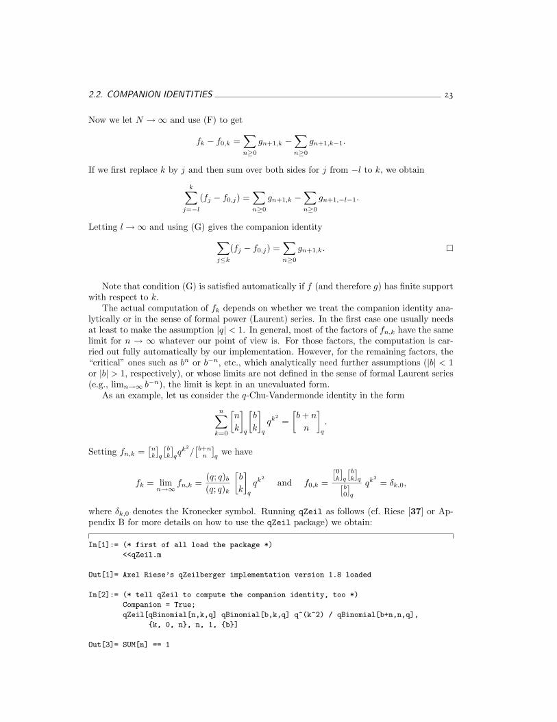
The actual computation of fk depends on whether we treat the companion identity ana-lytically or in the sense of formal power (Laurent) series. In the first case one usually needsat least to make the assumption |q| < 1. In general, most of the factors of fn,k have the samelimit for n → ∞ whatever our point of view is. For those factors, the computation is car-ried out fully automatically by our implementation. However, for the remaining factors, the“critical” ones such as bn or b−n, etc., which analytically need further assumptions (|b| < 1or |b| > 1, respectively), or whose limits are not defined in the sense of formal Laurent series(e.g., limn→∞ b−n), the limit is kept in an unevaluated form.
As an example, let us consider the q-Chu-Vandermonde identity in the form
n∑
k=0
[n
k
]
q
[b
k
]
q
qk2=
[b + n
n
]
q
.
Setting fn,k =[nk
]q
[bk
]qqk2
/[b+n
n
]q
we have
fk = limn→∞
fn,k =(q; q)b
(q; q)k
[b
k
]
q
qk2and f0,k =
[0k
]q
[bk
]q[
b0
]q
qk2= δk,0,
where δk,0 denotes the Kronecker symbol. Running qZeil as follows (cf. Riese [37] or Ap-pendix B for more details on how to use the qZeil package) we obtain:
In[1]:= (* first of all load the package *)
<<qZeil.m
Out[1]= Axel Riese’s qZeilberger implementation version 1.8 loaded
In[2]:= (* tell qZeil to compute the companion identity, too *)
Companion = True;
qZeil[qBinomial[n,k,q] qBinomial[b,k,q] q^(k^2) / qBinomial[b+n,n,q],
{k, 0, n}, n, 1, {b}]
Out[3]= SUM[n] == 1
24 CHAPTER 2. AUTOMATIC GENERATION OF q-IDENTITIES
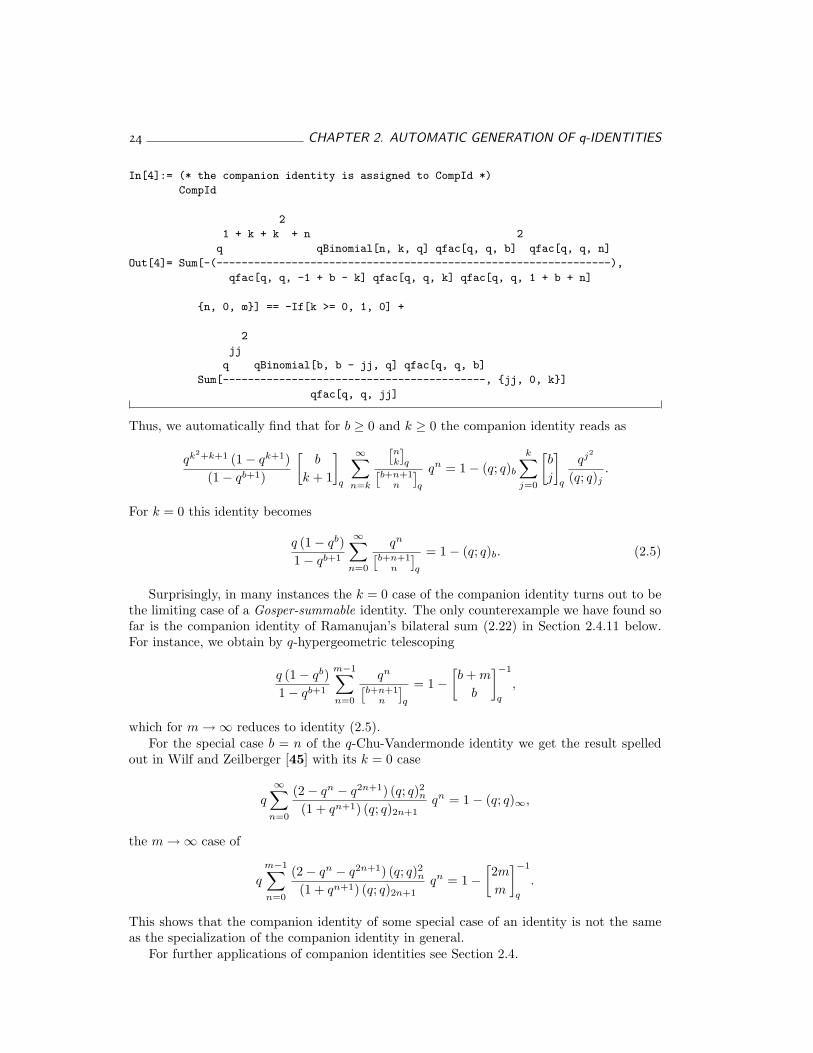
In[4]:= (* the companion identity is assigned to CompId *)
CompId
2
1 + k + k + n 2
q qBinomial[n, k, q] qfac[q, q, b] qfac[q, q, n]
Out[4]= Sum[−(−−−−−−−−−−−−−−−−−−−−−−−−−−−−−−−−−−−−−−−−−−−−−−−−−−−−−−−−−−−−−−−),
qfac[q, q, −1 + b − k] qfac[q, q, k] qfac[q, q, 1 + b + n]
{n, 0, ∞}] == −If[k >= 0, 1, 0] +
2
jj
q qBinomial[b, b − jj, q] qfac[q, q, b]
Sum[−−−−−−−−−−−−−−−−−−−−−−−−−−−−−−−−−−−−−−−−−−, {jj, 0, k}]
qfac[q, q, jj]
Thus, we automatically find that for b ≥ 0 and k ≥ 0 the companion identity reads as
qk2+k+1 (1− qk+1)(1− qb+1)
[b
k + 1
]
q
∞∑
n=k
[nk
]q[
b+n+1n
]q
qn = 1− (q; q)b
k∑
j=0
[b
j
]
q
qj2
(q; q)j.
For k = 0 this identity becomes
q (1− qb)1− qb+1
∞∑n=0
qn
[b+n+1
n
]q
= 1− (q; q)b. (2.5)
Surprisingly, in many instances the k = 0 case of the companion identity turns out to bethe limiting case of a Gosper-summable identity. The only counterexample we have found sofar is the companion identity of Ramanujan’s bilateral sum (2.22) in Section 2.4.11 below.For instance, we obtain by q-hypergeometric telescoping
q (1− qb)1− qb+1
m−1∑n=0
qn
[b+n+1
n
]q
= 1−[b + m
b
]−1
q
,
which for m →∞ reduces to identity (2.5).For the special case b = n of the q-Chu-Vandermonde identity we get the result spelled
out in Wilf and Zeilberger [45] with its k = 0 case
q
∞∑n=0
(2− qn − q2n+1) (q; q)2n(1 + qn+1) (q; q)2n+1
qn = 1− (q; q)∞,
the m →∞ case of
q
m−1∑n=0
(2− qn − q2n+1) (q; q)2n(1 + qn+1) (q; q)2n+1
qn = 1−[2m
m
]−1
q
.
This shows that the companion identity of some special case of an identity is not the sameas the specialization of the companion identity in general.
For further applications of companion identities see Section 2.4.
2.3. DUAL IDENTITIES 25
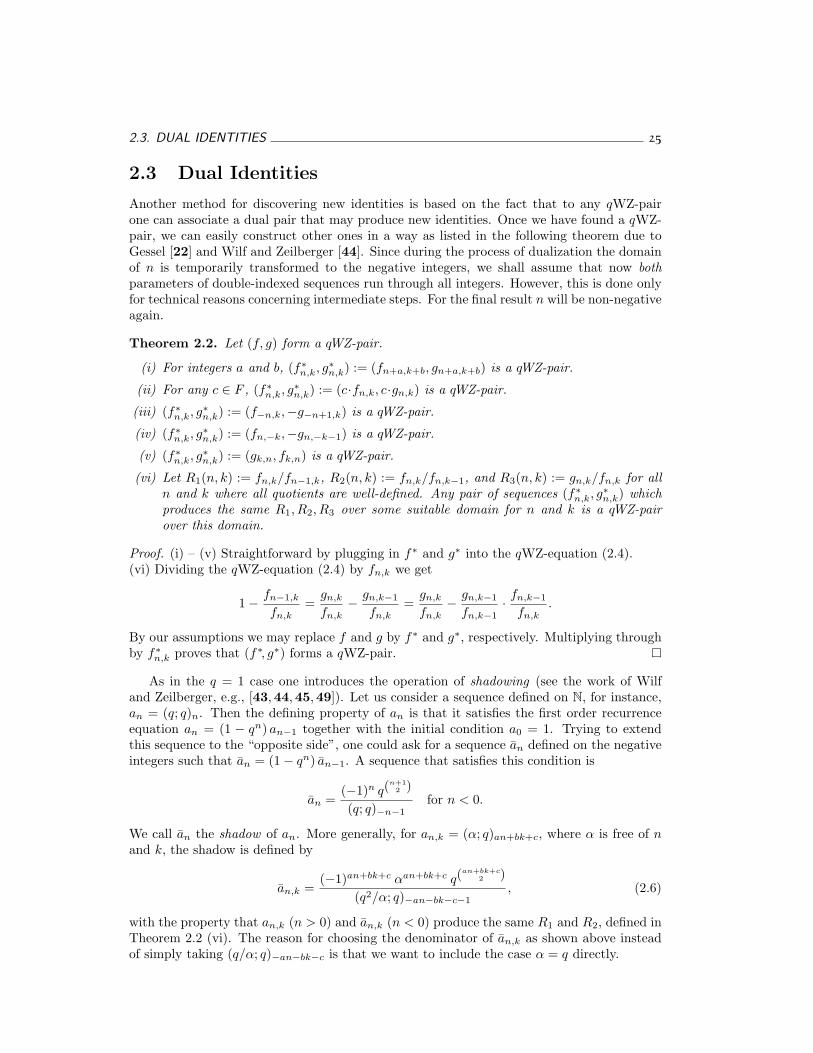
2.3 Dual Identities
Another method for discovering new identities is based on the fact that to any qWZ-pairone can associate a dual pair that may produce new identities. Once we have found a qWZ-pair, we can easily construct other ones in a way as listed in the following theorem due toGessel [22] and Wilf and Zeilberger [44]. Since during the process of dualization the domainof n is temporarily transformed to the negative integers, we shall assume that now bothparameters of double-indexed sequences run through all integers. However, this is done onlyfor technical reasons concerning intermediate steps. For the final result n will be non-negativeagain.
Theorem 2.2. Let (f, g) form a qWZ-pair.
(i) For integers a and b, (f∗n,k, g∗n,k) := (fn+a,k+b, gn+a,k+b) is a qWZ-pair.
(ii) For any c ∈ F , (f∗n,k, g∗n,k) := (c·fn,k, c·gn,k) is a qWZ-pair.
(iii) (f∗n,k, g∗n,k) := (f−n,k,−g−n+1,k) is a qWZ-pair.
(iv) (f∗n,k, g∗n,k) := (fn,−k,−gn,−k−1) is a qWZ-pair.
(v) (f∗n,k, g∗n,k) := (gk,n, fk,n) is a qWZ-pair.
(vi) Let R1(n, k) := fn,k/fn−1,k, R2(n, k) := fn,k/fn,k−1, and R3(n, k) := gn,k/fn,k for alln and k where all quotients are well-defined. Any pair of sequences (f∗n,k, g∗n,k) whichproduces the same R1, R2, R3 over some suitable domain for n and k is a qWZ-pairover this domain.
Proof. (i) – (v) Straightforward by plugging in f∗ and g∗ into the qWZ-equation (2.4).(vi) Dividing the qWZ-equation (2.4) by fn,k we get
1− fn−1,k
fn,k=
gn,k
fn,k− gn,k−1
fn,k=
gn,k
fn,k− gn,k−1
fn,k−1· fn,k−1
fn,k.
By our assumptions we may replace f and g by f∗ and g∗, respectively. Multiplying throughby f∗n,k proves that (f∗, g∗) forms a qWZ-pair.
As in the q = 1 case one introduces the operation of shadowing (see the work of Wilfand Zeilberger, e.g., [43,44,45,49]). Let us consider a sequence defined on N, for instance,an = (q; q)n. Then the defining property of an is that it satisfies the first order recurrenceequation an = (1 − qn) an−1 together with the initial condition a0 = 1. Trying to extendthis sequence to the “opposite side”, one could ask for a sequence an defined on the negativeintegers such that an = (1− qn) an−1. A sequence that satisfies this condition is
an =(−1)n q(
n+12 )
(q; q)−n−1for n < 0.
We call an the shadow of an. More generally, for an,k = (α; q)an+bk+c, where α is free of nand k, the shadow is defined by
an,k =(−1)an+bk+c αan+bk+c q(
an+bk+c2 )
(q2/α; q)−an−bk−c−1, (2.6)
with the property that an,k (n > 0) and an,k (n < 0) produce the same R1 and R2, defined inTheorem 2.2 (vi). The reason for choosing the denominator of an,k as shown above insteadof simply taking (q/α; q)−an−bk−c is that we want to include the case α = q directly.
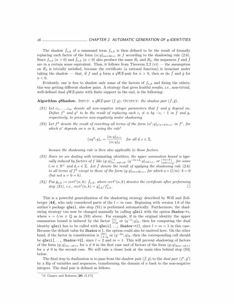
26 CHAPTER 2. AUTOMATIC GENERATION OF q-IDENTITIES
The shadow fn,k of a summand term fn,k is then defined to be the result of formallyreplacing each factor of the form (α; q)an+bk+c in f according to the shadowing rule (2.6).Since fn,k (n > 0) and fn,k (n < 0) also produce the same R1 and R2, the sequences f and fare in a certain sense equivalent. Thus, it follows from Theorem 2.2 (vi) — the assumptionon R3 is trivially satisfied, because the certificate (a rational function) is invariant undertaking the shadow — that, if f and g form a qWZ-pair for n > 0, then so do f and g forn < 0.
Evidently, one is free to shadow only some of the factors of fn,k and fixing the others,this way getting different shadow pairs. A strategy that gives fruitful results, i.e., non-trivial,well-defined dual qWZ-pairs with finite support in the end, is the following:
Algorithm qShadow. Input: a qWZ-pair (f, g); Output: the shadow pair (f , g).
(S1) Let c1, . . . , cm denote all non-negative integer parameters that f and g depend on.Define f1 and g1 to be the result of replacing each ci 6= n by −ci − 1 in f and g,respectively, to preserve non-negativity under shadowing.
(S2) Let f2 denote the result of rewriting all terms of the form (α′; q)a′n+b′k+c′ in f1, forwhich α′ depends on n or k, using the rule†
(αqd; q)e =(α; q)d+e
(α; q)dfor all d, e ∈ Z,
because the shadowing rule is then also applicable to those factors.
(S3) Since we are dealing with terminating identities, the upper summation bound is typi-cally induced by factors of f like (q; q)−1
ln−mk+d, (q−ln+d; q)mk+e, or[
ln+dmk+e
]q, for some
l, m ∈ N+ and d, e ∈ Z. Let f denote the result of applying the shadowing rule (2.6)to all terms of f2 except to those of the form (q; q)an+bk+c, for which a+(l/m) · b = 0(but not a = 0 = b).
(S4) Put gn,k := cert1(n, k) · fn,k, where cert1(n, k) denotes the certificate after performingstep (S1), i.e., cert1(n, k) = g1
n,k/f1n,k.
This is a powerful generalization of the shadowing strategy described by Wilf and Zeil-berger [44], who only considered parts of the l = m case. Beginning with version 1.6 of theauthor’s package qZeil, also step (S1) is performed automatically. Furthermore, the shad-owing strategy can now be changed manually by calling qZeil with the option Shadow->s,where s = l/m ∈ Q as in (S3) above. For example, if in the original identity the uppersummation bound is induced by the factor
[nk
]q
or (q−n; q)k, then for computing the dualidentity qZeil has to be called with qZeil[. . . , Shadow->1], since l = m = 1 in this case.Because the default value for Shadow is 1, the option could also be omitted here. On the otherhand, if the factor in consideration is
[2nk
]q
or (q−2n; q)k, then the corresponding call shouldbe qZeil[. . . , Shadow->2], since l = 2 and m = 1. This will prevent shadowing of factorsof the form (q; q)an−ak+c for a 6= 0 in the first case and of factors of the form (q; q)2an−ak+c
for a 6= 0 in the second case. We will take a closer look at the main idea behind step (S3)below.
The final step in dualization is to pass from the shadow pair (f , g) to the dual pair (f ′, g′)by a flip of variables and sequences, transforming the domain of n back to the non-negativeintegers. The dual pair is defined as follows.
†cf. Gasper and Rahman [20, (I.17)]
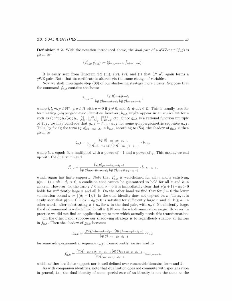
2.3. DUAL IDENTITIES 27
Definition 2.2. With the notation introduced above, the dual pair of a qWZ-pair (f, g) isgiven by
(f ′n,k, g′n,k) := (g−k,−n−1, f−k−1,−n).
It is easily seen from Theorem 2.2 (iii), (iv), (v), and (i) that (f ′, g′) again forms aqWZ-pair. Note that its certificate is altered via the same change of variables.
Now we shall investigate step (S3) of our shadowing strategy more closely. Suppose thatthe summand fn,k contains the factor
hn,k =(q; q)in+jk+d1
(q; q)ln−mk+d2 (q; q)on+pk+d3
,
where i, l, m, p ∈ N+, j, o ∈ N with o = 0 if j 6= 0, and d1, d2, d3 ∈ Z. This is usually true forterminating q-hypergeometric identities, however, hn,k might appear in an equivalent formsuch as (q−n; q)k/(q; q)k,
[nk
]q,[
2nn−k
]q,[n+k2k
]q, etc. Since gn,k is a rational function multiple
of fn,k, we may conclude that gn,k = hn,k · an,k for some q-hypergeometric sequence an,k.Thus, by fixing the term (q; q)ln−mk+d2 in hn,k, according to (S3), the shadow of gn,k is thengiven by
gn,k =(q; q)−on−pk−d3−1
(q; q)ln−mk+d2 (q; q)−in−jk−d1−1· bn,k,
where bn,k equals an,k multiplied with a power of −1 and a power of q. This means, we endup with the dual summand
f ′n,k =(q; q)pn+ok+p−d3−1
(q; q)mn−lk+m+d2 (q; q)jn+ik+j−d1−1· b−k,−n−1,
which again has finite support. Note that f ′n,k is well-defined for all n and k satisfyingp(n + 1) + ok − d3 > 0, a condition that cannot be guaranteed to hold for all n and k ingeneral. However, for the case j 6= 0 and o = 0 it is immediately clear that p(n + 1)− d3 > 0holds for sufficiently large n and all k. On the other hand we find that for j = 0 the lowersummation bound a := d(d1 + 1)/ie in the dual identity does not depend on n. Thus, it iseasily seen that p(n + 1) + ok − d3 > 0 is satisfied for sufficiently large n and all k ≥ a. Inother words, after substituting n + n0 for n in the dual pair, with n0 ∈ N sufficiently large,the dual summand is well-defined for all n ∈ N over the whole summation range. However, inpractice we did not find an application up to now which actually needs this transformation.
On the other hand, suppose our shadowing strategy is to regardlessly shadow all factorsin fn,k. Then the shadow of gn,k becomes
gn,k =(q; q)−ln+mk−d2−1 (q; q)−on−pk−d3−1
(q; q)−in−jk−d1−1· cn,k
for some q-hypergeometric sequence cn,k. Consequently, we are lead to
f ′n,k =(q; q)−mn+lk−m−d2−1 (q; q)pn+ok+p−d3−1
(q; q)jn+ik+j−d1−1· c−k,−n−1,
which neither has finite support nor is well-defined over reasonable domains for n and k.As with companion identities, note that dualization does not commute with specialization
in general, i.e., the dual identity of some special case of an identity is not the same as the
28 CHAPTER 2. AUTOMATIC GENERATION OF q-IDENTITIES
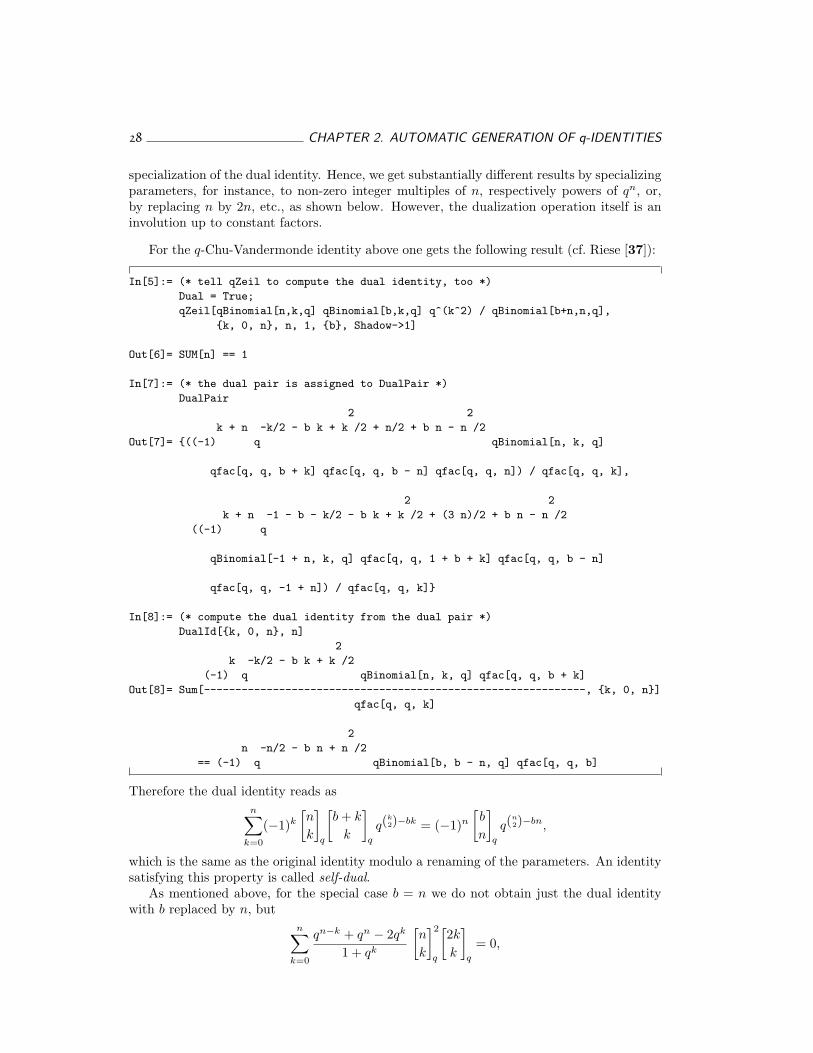
specialization of the dual identity. Hence, we get substantially different results by specializingparameters, for instance, to non-zero integer multiples of n, respectively powers of qn, or,by replacing n by 2n, etc., as shown below. However, the dualization operation itself is aninvolution up to constant factors.
For the q-Chu-Vandermonde identity above one gets the following result (cf. Riese [37]):
In[5]:= (* tell qZeil to compute the dual identity, too *)
Dual = True;
qZeil[qBinomial[n,k,q] qBinomial[b,k,q] q^(k^2) / qBinomial[b+n,n,q],
{k, 0, n}, n, 1, {b}, Shadow->1]
Out[6]= SUM[n] == 1
In[7]:= (* the dual pair is assigned to DualPair *)
DualPair
2 2
k + n -k/2 - b k + k /2 + n/2 + b n - n /2
Out[7]= {((-1) q qBinomial[n, k, q]
qfac[q, q, b + k] qfac[q, q, b - n] qfac[q, q, n]) / qfac[q, q, k],
2 2
k + n -1 - b - k/2 - b k + k /2 + (3 n)/2 + b n - n /2
((-1) q
qBinomial[-1 + n, k, q] qfac[q, q, 1 + b + k] qfac[q, q, b - n]
qfac[q, q, -1 + n]) / qfac[q, q, k]}
In[8]:= (* compute the dual identity from the dual pair *)
DualId[{k, 0, n}, n]
2
k -k/2 - b k + k /2
(-1) q qBinomial[n, k, q] qfac[q, q, b + k]
Out[8]= Sum[-------------------------------------------------------------, {k, 0, n}]
qfac[q, q, k]
2
n -n/2 - b n + n /2
== (-1) q qBinomial[b, b - n, q] qfac[q, q, b]
Therefore the dual identity reads asn∑
k=0
(−1)k
[n
k
]
q
[b + k
k
]
q
q(k2)−bk = (−1)n
[b
n
]
q
q(n2)−bn,
which is the same as the original identity modulo a renaming of the parameters. An identitysatisfying this property is called self-dual.
As mentioned above, for the special case b = n we do not obtain just the dual identitywith b replaced by n, but
n∑
k=0
qn−k + qn − 2qk
1 + qk
[n
k
]2
q
[2k
k
]
q
= 0,
2.4. APPLICATIONS 29
presented by Wilf and Zeilberger [45].Next, let us consider the q-Saalschutz identity in the form
n∑
k=0
[r − s + m
k
]
q
[s− r + n
n− k
]
q
[s + k
m + n
]
q
q(n−k)(r−s+m−k) =[r
n
]
q
[s
m
]
q
.
The program computes the following dual identity (cf. Riese [37]):
n∑
k=0
[m + k
k
]
q
[s
r − k
]
q
[m− s
n− k
]
q
q(n−k)(r−k) =[m + r − s
n
]
q
[n + s
r
]
q
.
Renaming the parameters we find the q-Saalschutz identity also to be self-dual.For the special case m = n and r = s, the process of dualization leads to the following
result (cf. Riese [37]):
n∑
k=0
(2qn − qk − qk+n−s − q2k − q2k+n−s + 2q3k−s) (q; q)n+s−2k−1
(1 + qk) (q; q)2s−k
[n
k
]2
q
[2k
k
]
q
q−2k = 0,
where s ≥ n + 1.Further applications of dual identities are given in the following section.
2.4 Applications
In the following we shall present several dual and companion identities of “standard” ter-minating q-identities taken from Appendix II of Gasper and Rahman [20]. Unfortunately,it turned out that the full power of Gessel’s [22] method for systematically producing dualidentities in the q = 1 case cannot be carried over to the q-case completely, since factoriza-tion of q-polynomials (where the variables occur as exponents of q) is much harder to handlealgorithmically than the q = 1 case.
Recall the usual definitions of an rφs basic hypergeometric series
rφs(a1, a2, . . . , ar; b1, . . . , bs; q, z) ≡ rφs
[a1, a2, . . . , ar
b1, . . . , bs; q, z
]
:=∞∑
k=0
(a1, a2, . . . , ar; q)k
(q, b1, . . . , bs; q)k
((−1)k q(
k2)
)1+s−r
zk,
and an rψs basic bilateral hypergeometric series
rψs(a1, a2, . . . , ar; b1, b2, . . . , bs; q, z) ≡ rψs
[a1, a2, . . . , ar
b1, b2, . . . , bs; q, z
]
:=∞∑
k=−∞
(a1, a2, . . . , ar; q)k
(b1, b2, . . . , bs; q)k
((−1)k q(
k2)
)s−r
zk.
All finite versions of companion identities for k = 0 have been found algorithmically byq-hypergeometric telescoping. Krattenthaler [26] kindly pointed out many connections be-tween several identities to me.
30 CHAPTER 2. AUTOMATIC GENERATION OF q-IDENTITIES
2.4.1 The q-Binomial Theorem
From the q-binomial theorem [20, (II.4)],
1φ0(q−n,—; q, z) = (zq−n; q)n, (2.7)
we obtain the dual identity
2φ1(q−n, z; 0; q, q) = zn,
which is a special case of the q-Chu-Vandermonde identity [20, (II.6)]. The companionidentity after replacing z by −q/z is a special case of the 1φ1 summation formula (2.8) below,
(−q/z)k
(q; q)k
∞∑
n=k
zn (q−n; q)k
(−z; q)n+1q(
n2) = 1 (k ≥ 0),
which for k = 0 reduces to the m →∞ case of
m−1∑n=0
zn q(n2)
(−z; q)n+1= 1− zm q(
m2 )
(−z; q)m.
For z = −q and z = q we immediately get
m∑n=0
(−1)n q(n2)
(q; q)n=
(−1)m q(m+1
2 )
(q; q)mand
m∑n=0
q(n2)
(−q; q)n= 2− q(
m+12 )
(−q; q)m,
respectively, with the limiting cases
∞∑n=0
(−1)n q(n2)
(q; q)n= 0 and
∞∑n=0
q(n2)
(−q; q)n= 2,
respectively. The first identity is a special case of Euler’s q-analogue of the exponentialfunction (cf. Andrews [7]), whereas the second one was derived by Andrews [5] in the contextof mock-theta-functions. The dual identity of (2.7) for z = q−n reads as
2n∑
k=0
(−1)k (qk + q2k − qn)(1 + qk) (q; q)n−k
[2k
k
]
q
q(k2)−2nk =
qn
(q; q)n.
The companion identity of (2.7) for z = q−n is
q−k
(q; q)k
∞∑
n=k
(−1)n (qk + qn+k+1 − q2n+1) (q−n; q)k
(qn+2; q)n+1qn(3n−2k+1)/2 = 1 (k ≥ 0),
which for k = 0 reduces to the m →∞ case of
m−1∑n=0
(−1)n (1 + qn+1 − q2n+1)(qn+2; q)n+1
qn(3n+1)/2 = 1− (−1)m qm(3m+1)/2
(qm+1; q)m.
2.4. APPLICATIONS 31
2.4.2 The Sum of a 1φ1 Series
The sum of a 1φ1 series [20, (II.5)],
1φ1(a; c; q, c/a) =(c/a; q)∞(c; q)∞
, (2.8)
turns out to be self-dual for a = q−n. The companion identity in this case is
(−1)k ck+1 q(k+12 )
(c, q; q)k
∞∑
n=k
(q−n; q)k (c; q)n qn(k+1) =
1− (c; q)∞k∑
j=0
cj qj(j−1)
(c, q; q)j(k ≥ 0), (2.9)
which for k = 0 reduces to the m →∞ case of
c
m−1∑n=0
(c; q)n qn = 1− (c; q)m. (2.10)
Apparently, identity (2.10) — despite its simplicity — has not been included into the q-hyper-geometric database in this form up to now. However, this result can also be derived fromthe original 1φ1 summation formula. Letting k →∞ in (2.9) we obtain
∞∑
j=0
cj qj(j−1)
(c, q; q)j=
1(c; q)∞
,
which is known as Cauchy’s formula (cf., for instance, Andrews [7]). Note that letting k →∞in the companion identity, in general corresponds to letting n → ∞ in the original identity.The dual identity of (2.8) for a = q−n and c = qn reads as
n∑
k=0
(1− q2k+2 − q2k+n+2 + q3k+2) (q; q)k+n+1
(q; q)2k+2
[n
k
]
q
qk(2k+1) = 1,
which for n →∞ becomes∞∑
k=0
qk(2k+1)
(q; q)2k+1 (q; q)k=
1(q; q)∞
− q2∞∑
k=0
q2k(k+2)
(q; q)2k+2 (q; q)k.
The companion identity does not exist in this case because the limit involved is not finite.
2.4.3 The q-Chu-Vandermonde Identity
From the q-Chu-Vandermonde identity [20, (II.7)],
2φ1(a, q−n; c; q, cqn/a) =(c/a; q)n
(c; q)n, (2.11)
we obtain the dual identity
2φ1(aq/c, q−n; q2/c; q, q1+n/a) =(q/a; q)n
(q2/c; q)n,
32 CHAPTER 2. AUTOMATIC GENERATION OF q-IDENTITIES
which is again q-Chu-Vandermonde. The companion identity is
ak+1 (c/a; q)k+1
(c, q; q)k
∞∑
n=k
(q−n; q)k (c; q)n
(a; q)n+1qn(k+1)
=(c; q)∞(a; q)∞
k∑
j=0
(−1)j aj (c/a; q)j
(c, q; q)jq(
j2) − 1 (k ≥ 0),
which for k → ∞ turns into the 1φ1 summation formula (2.8) above and for k = 0 reducesto the m →∞ case of
a (1− c/a)m−1∑n=0
(c; q)n qn
(a; q)n+1=
(c; q)m
(a; q)m− 1.
For a = 0 this identity again gives equation (2.9), whereas the case c = 0 leads to the likewisesimple result
am−1∑n=0
qn
(a; q)n+1=
1(a; q)m
− 1, (2.12)
an extended version of the well-known identity
m∑n=0
qn
(q; q)n=
1(q; q)m
.
The dual identity of (2.11) for a = qn reads as
n∑
k=−n−1
ck (q2/c; q)k
(c; q)k
[2n + 1n− k
]
q
qk(k−1) =(qn+1; q)n+1
(c; q)n, (2.13)
a special case of Carlitz’ [18] summation formula
3φ2
[q−2n−1, b, c
q−2n/b, q−2n/c; q,
q2−n
bc
]=
(bq, cq; q)n (q2, bcq; q)2n
(q2, bcq; q)n (bq, cq; q)2n. (2.14)
Identity (2.13) turns out to be of special interest in the frame of Bailey chains (see, e.g.,Andrews [10], or Paule [30]). For instance, for c = 0 we obtain
n∑
k=−n−1
(−1)k
[2n + 1n− k
]
q
qk(3k+1)/2 = (qn+1; q)n+1,
the unsymmetric counterpart of the Bailey pair identity (cf. Paule [30])
n∑
k=−n
(−1)k
[2n
n− k
]
q
qk(3k+1)/2 = (qn+1; q)n.
In the limit n → ∞ both identities turn into Euler’s pentagonal number theorem (see, e.g.,Andrews [7])
∞∑
k=−∞(−1)k qk(3k+1)/2 = (q; q)∞.
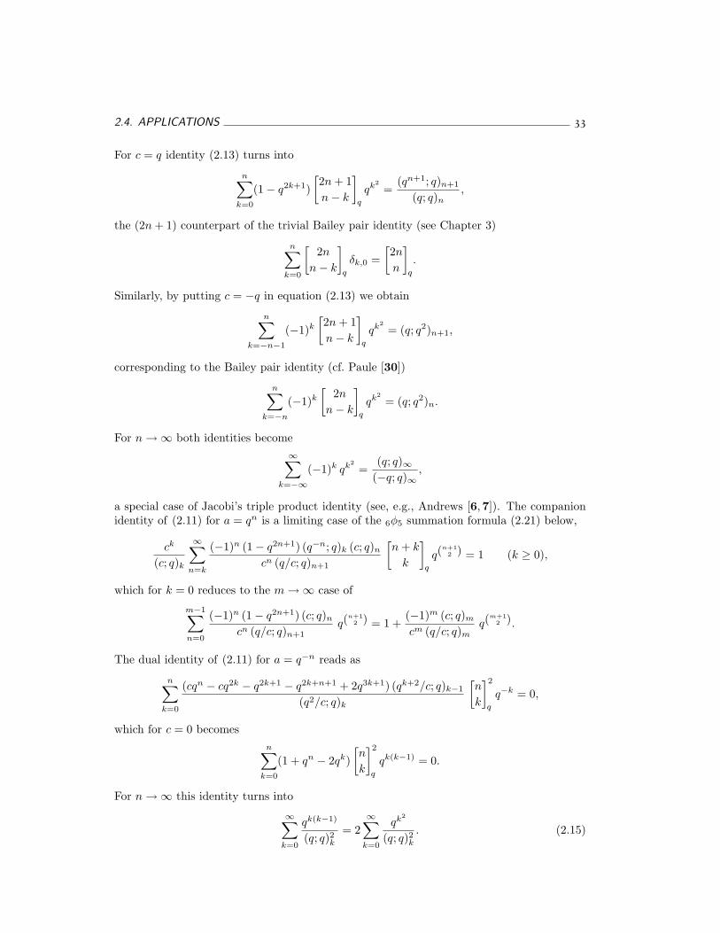
2.4. APPLICATIONS 33
For c = q identity (2.13) turns into
n∑
k=0
(1− q2k+1)[2n + 1n− k
]
q
qk2=
(qn+1; q)n+1
(q; q)n,
the (2n + 1) counterpart of the trivial Bailey pair identity (see Chapter 3)
n∑
k=0
[2n
n− k
]
q
δk,0 =[2n
n
]
q
.
Similarly, by putting c = −q in equation (2.13) we obtain
n∑
k=−n−1
(−1)k
[2n + 1n− k
]
q
qk2= (q; q2)n+1,
corresponding to the Bailey pair identity (cf. Paule [30])
n∑
k=−n
(−1)k
[2n
n− k
]
q
qk2= (q; q2)n.
For n →∞ both identities become∞∑
k=−∞(−1)k qk2
=(q; q)∞
(−q; q)∞,
a special case of Jacobi’s triple product identity (see, e.g., Andrews [6,7]). The companionidentity of (2.11) for a = qn is a limiting case of the 6φ5 summation formula (2.21) below,
ck
(c; q)k
∞∑
n=k
(−1)n (1− q2n+1) (q−n; q)k (c; q)n
cn (q/c; q)n+1
[n + k
k
]
q
q(n+1
2 ) = 1 (k ≥ 0),
which for k = 0 reduces to the m →∞ case of
m−1∑n=0
(−1)n (1− q2n+1) (c; q)n
cn (q/c; q)n+1q(
n+12 ) = 1 +
(−1)m (c; q)m
cm (q/c; q)mq(
m+12 ).
The dual identity of (2.11) for a = q−n reads as
n∑
k=0
(cqn − cq2k − q2k+1 − q2k+n+1 + 2q3k+1) (qk+2/c; q)k−1
(q2/c; q)k
[n
k
]2
q
q−k = 0,
which for c = 0 becomesn∑
k=0
(1 + qn − 2qk)[n
k
]2
q
qk(k−1) = 0.
For n →∞ this identity turns into
∞∑
k=0
qk(k−1)
(q; q)2k= 2
∞∑
k=0
qk2
(q; q)2k. (2.15)
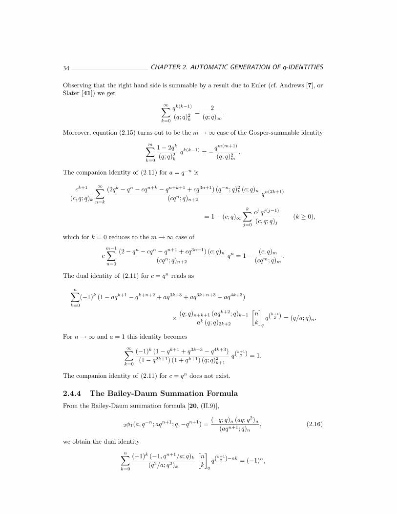
34 CHAPTER 2. AUTOMATIC GENERATION OF q-IDENTITIES
Observing that the right hand side is summable by a result due to Euler (cf. Andrews [7], orSlater [41]) we get
∞∑
k=0
qk(k−1)
(q; q)2k=
2(q; q)∞
.
Moreover, equation (2.15) turns out to be the m →∞ case of the Gosper-summable identity
m∑
k=0
1− 2qk
(q; q)2kqk(k−1) = −qm(m+1)
(q; q)2m.
The companion identity of (2.11) for a = q−n is
ck+1
(c, q; q)k
∞∑
n=k
(2qk − qn − cqn+k − qn+k+1 + cq3n+1) (q−n; q)2k (c; q)n
(cqn; q)n+2qn(2k+1)
= 1− (c; q)∞k∑
j=0
cj qj(j−1)
(c, q; q)j(k ≥ 0),
which for k = 0 reduces to the m →∞ case of
c
m−1∑n=0
(2− qn − cqn − qn+1 + cq3n+1) (c; q)n
(cqn; q)n+2qn = 1− (c; q)m
(cqm; q)m.
The dual identity of (2.11) for c = qn reads as
n∑
k=0
(−1)k (1− aqk+1 − qk+n+2 + aq3k+3 + aq3k+n+3 − aq4k+3)
× (q; q)n+k+1 (aqk+2; q)k−1
ak (q; q)2k+2
[n
k
]
q
q(k+12 ) = (q/a; q)n.
For n →∞ and a = 1 this identity becomes
∞∑
k=0
(−1)k (1− qk+1 + q3k+3 − q4k+3)(1− q2k+1) (1 + qk+1) (q; q)2k+1
q(k+12 ) = 1.
The companion identity of (2.11) for c = qn does not exist.
2.4.4 The Bailey-Daum Summation Formula
From the Bailey-Daum summation formula [20, (II.9)],
2φ1(a, q−n; aqn+1; q,−qn+1) =(−q; q)n (aq; q2)n
(aqn+1; q)n, (2.16)
we obtain the dual identity
n∑
k=0
(−1)k (−1, qn+1/a; q)k
(q2/a; q2)k
[n
k
]
q
q(k+12 )−nk = (−1)n,
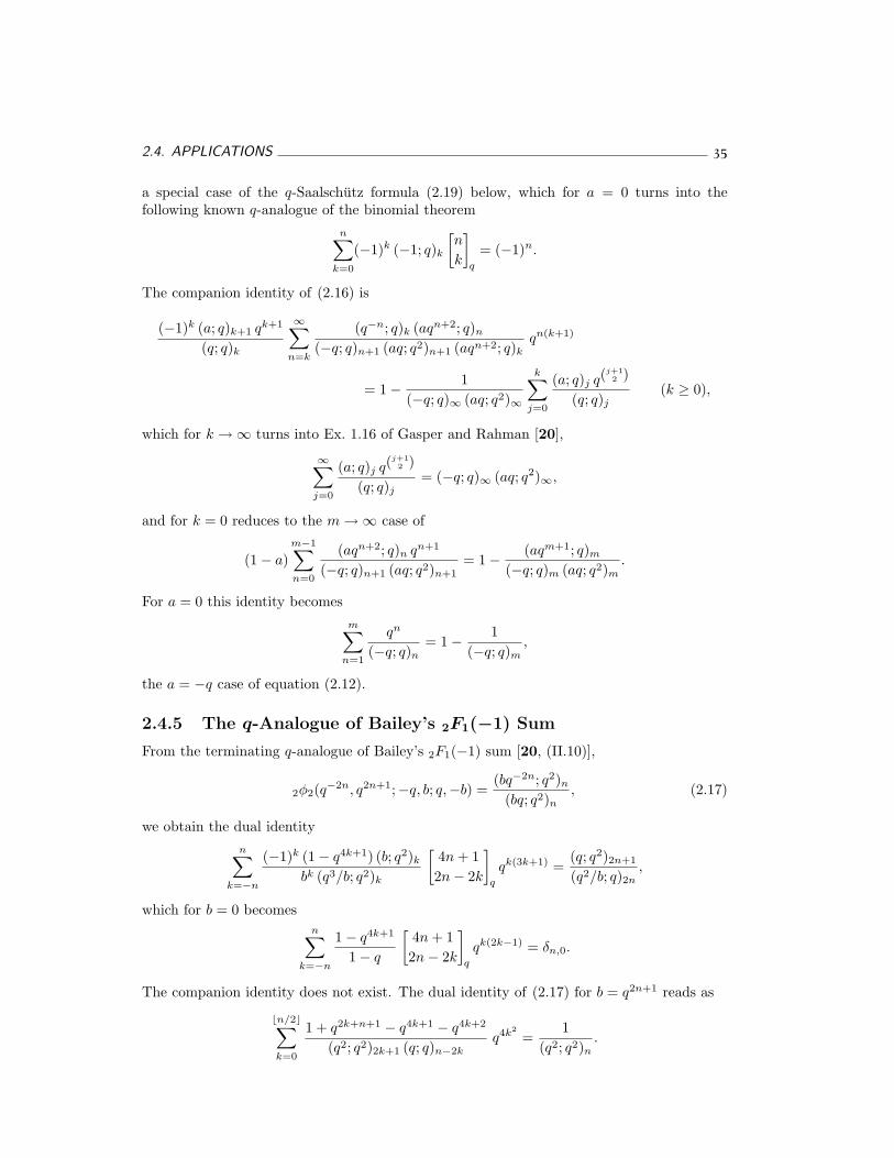
2.4. APPLICATIONS 35
a special case of the q-Saalschutz formula (2.19) below, which for a = 0 turns into thefollowing known q-analogue of the binomial theorem
n∑
k=0
(−1)k (−1; q)k
[n
k
]
q
= (−1)n.
The companion identity of (2.16) is
(−1)k (a; q)k+1 qk+1
(q; q)k
∞∑
n=k
(q−n; q)k (aqn+2; q)n
(−q; q)n+1 (aq; q2)n+1 (aqn+2; q)kqn(k+1)
= 1− 1(−q; q)∞ (aq; q2)∞
k∑
j=0
(a; q)j q(j+12 )
(q; q)j(k ≥ 0),
which for k →∞ turns into Ex. 1.16 of Gasper and Rahman [20],
∞∑
j=0
(a; q)j q(j+12 )
(q; q)j= (−q; q)∞ (aq; q2)∞,
and for k = 0 reduces to the m →∞ case of
(1− a)m−1∑n=0
(aqn+2; q)n qn+1
(−q; q)n+1 (aq; q2)n+1= 1− (aqm+1; q)m
(−q; q)m (aq; q2)m.
For a = 0 this identity becomesm∑
n=1
qn
(−q; q)n= 1− 1
(−q; q)m,
the a = −q case of equation (2.12).
2.4.5 The q-Analogue of Bailey’s 2F1(−1) Sum
From the terminating q-analogue of Bailey’s 2F1(−1) sum [20, (II.10)],
2φ2(q−2n, q2n+1;−q, b; q,−b) =(bq−2n; q2)n
(bq; q2)n, (2.17)
we obtain the dual identityn∑
k=−n
(−1)k (1− q4k+1) (b; q2)k
bk (q3/b; q2)k
[4n + 12n− 2k
]
q
qk(3k+1) =(q; q2)2n+1
(q2/b; q)2n,
which for b = 0 becomesn∑
k=−n
1− q4k+1
1− q
[4n + 12n− 2k
]
q
qk(2k−1) = δn,0.
The companion identity does not exist. The dual identity of (2.17) for b = q2n+1 reads as
bn/2c∑
k=0
1 + q2k+n+1 − q4k+1 − q4k+2
(q2; q2)2k+1 (q; q)n−2kq4k2
=1
(q2; q2)n.
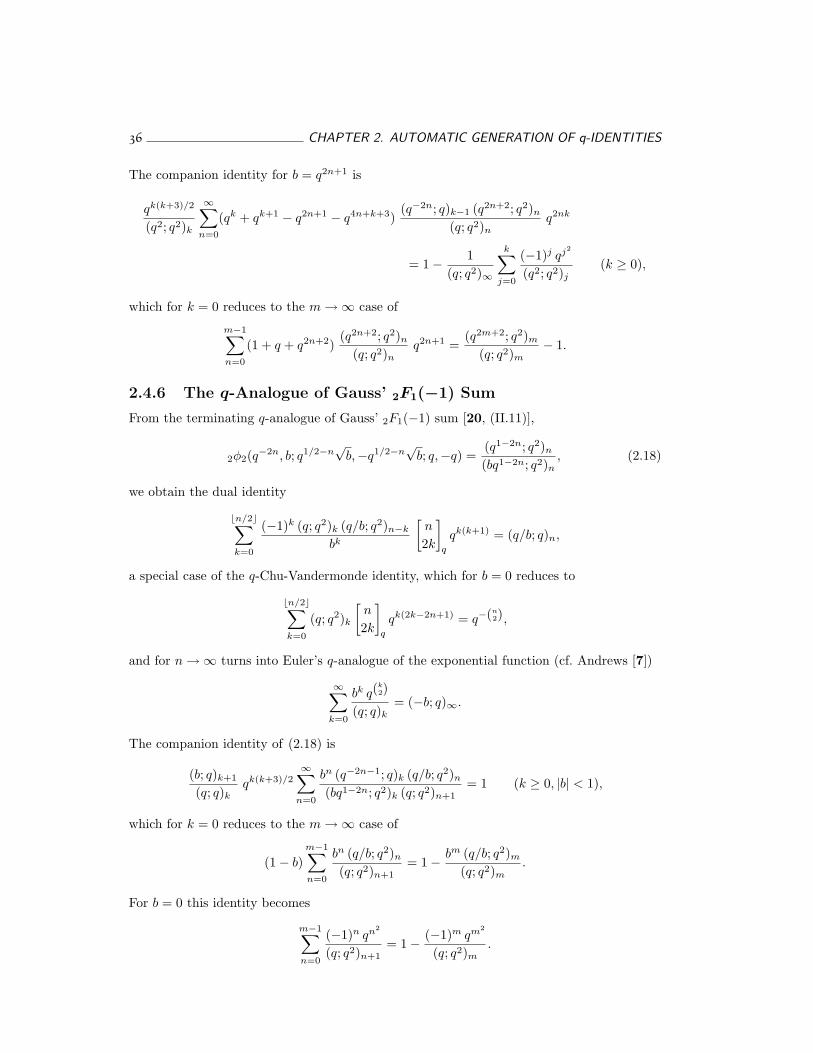
36 CHAPTER 2. AUTOMATIC GENERATION OF q-IDENTITIES
The companion identity for b = q2n+1 is
qk(k+3)/2
(q2; q2)k
∞∑n=0
(qk + qk+1 − q2n+1 − q4n+k+3)(q−2n; q)k−1 (q2n+2; q2)n
(q; q2)nq2nk
= 1− 1(q; q2)∞
k∑
j=0
(−1)j qj2
(q2; q2)j(k ≥ 0),
which for k = 0 reduces to the m →∞ case of
m−1∑n=0
(1 + q + q2n+2)(q2n+2; q2)n
(q; q2)nq2n+1 =
(q2m+2; q2)m
(q; q2)m− 1.
2.4.6 The q-Analogue of Gauss’ 2F1(−1) Sum
From the terminating q-analogue of Gauss’ 2F1(−1) sum [20, (II.11)],
2φ2(q−2n, b; q1/2−n√
b,−q1/2−n√
b; q,−q) =(q1−2n; q2)n
(bq1−2n; q2)n, (2.18)
we obtain the dual identity
bn/2c∑
k=0
(−1)k (q; q2)k (q/b; q2)n−k
bk
[n
2k
]
q
qk(k+1) = (q/b; q)n,
a special case of the q-Chu-Vandermonde identity, which for b = 0 reduces to
bn/2c∑
k=0
(q; q2)k
[n
2k
]
q
qk(2k−2n+1) = q−(n2),
and for n →∞ turns into Euler’s q-analogue of the exponential function (cf. Andrews [7])
∞∑
k=0
bk q(k2)
(q; q)k= (−b; q)∞.
The companion identity of (2.18) is
(b; q)k+1
(q; q)kqk(k+3)/2
∞∑n=0
bn (q−2n−1; q)k (q/b; q2)n
(bq1−2n; q2)k (q; q2)n+1= 1 (k ≥ 0, |b| < 1),
which for k = 0 reduces to the m →∞ case of
(1− b)m−1∑n=0
bn (q/b; q2)n
(q; q2)n+1= 1− bm (q/b; q2)m
(q; q2)m.
For b = 0 this identity becomes
m−1∑n=0
(−1)n qn2
(q; q2)n+1= 1− (−1)m qm2
(q; q2)m.
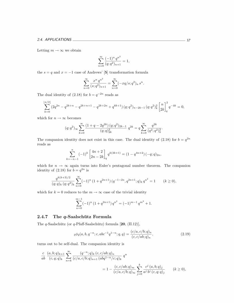
2.4. APPLICATIONS 37
Letting m →∞ we obtain
∞∑n=0
(−1)n qn2
(q; q2)n+1= 1,
the s = q and x = −1 case of Andrews’ [5] transformation formula
∞∑n=0
xn qn2
(s; q2)n+1=
∞∑n=0
(−xq/s; q2)n sn.
The dual identity of (2.18) for b = q−2n reads as
bn/2c∑
k=0
(2q2n − q2k+n − q2k+n+1 − q2k+2n + q6k+1) (q; q2)n−2k−1 (q; q2)2k
[n
2k
]2
q
q−4k = 0,
which for n →∞ becomes
(q; q2)∞∞∑
k=0
(1 + q − 2q2k) (q; q2)2k−1
(q; q)22k
q2k = q
∞∑
k=0
q2k
(q2; q2)2k.
The companion identity does not exist in this case. The dual identity of (2.18) for b = q2n
reads asn∑
k=−n−1
(−1)k
[4n + 22n− 2k
]
q
qk(3k+1) = (1− q4n+2) (−q; q)2n,
which for n → ∞ again turns into Euler’s pentagonal number theorem. The companionidentity of (2.18) for b = q2n is
qk(k+3)/2
(q; q)k (q; q2)k
∞∑n=0
(−1)n (1 + q2n+1) (q−1−2n, q2n+1; q)k qn2= 1 (k ≥ 0),
which for k = 0 reduces to the m →∞ case of the trivial identity
m−1∑n=0
(−1)n (1 + q2n+1) qn2= (−1)m−1 qm2
+ 1.
2.4.7 The q-Saalschutz Formula
The q-Saalschutz (or q-Pfaff-Saalschutz) formula [20, (II.12)],
3φ2(a, b, q−n; c, abc−1q1−n; q, q) =(c/a, c/b; q)n
(c, c/ab; q)n, (2.19)
turns out to be self-dual. The companion identity is
c
ab
(a, b; q)k+1
(c, q; q)k
∞∑
n=k
(q−n; q)k (c, c/ab; q)n
(c/a, c/b; q)n+1 (abq1−n/c; q)kqn
= 1− (c, c/ab; q)∞(c/a, c/b; q)∞
k∑
j=0
cj (a, b; q)j
aj bj (c, q; q)j(k ≥ 0),
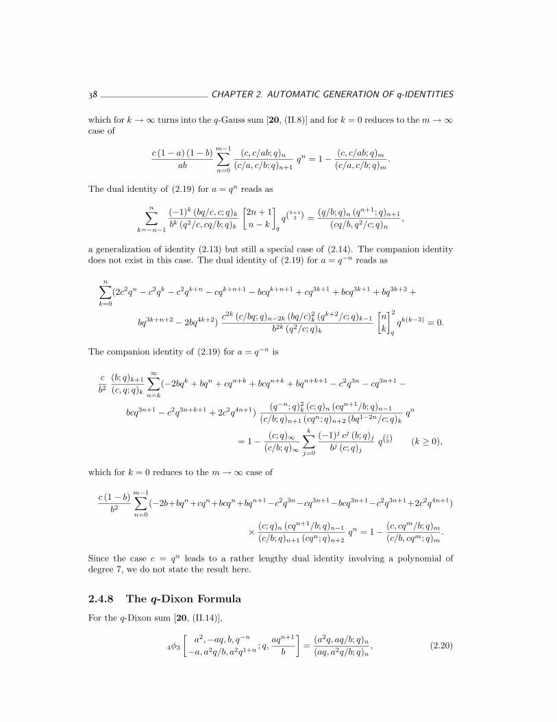
38 CHAPTER 2. AUTOMATIC GENERATION OF q-IDENTITIES
which for k →∞ turns into the q-Gauss sum [20, (II.8)] and for k = 0 reduces to the m →∞case of
c (1− a) (1− b)ab
m−1∑n=0
(c, c/ab; q)n
(c/a, c/b; q)n+1qn = 1− (c, c/ab; q)m
(c/a, c/b; q)m.
The dual identity of (2.19) for a = qn reads as
n∑
k=−n−1
(−1)k (bq/c, c; q)k
bk (q2/c, cq/b; q)k
[2n + 1n− k
]
q
q(k+12 ) =
(q/b; q)n (qn+1; q)n+1
(cq/b, q2/c; q)n,
a generalization of identity (2.13) but still a special case of (2.14). The companion identitydoes not exist in this case. The dual identity of (2.19) for a = q−n reads as
n∑
k=0
(2c2qn − c2qk − c2qk+n − cqk+n+1 − bcqk+n+1 + cq3k+1 + bcq3k+1 + bq3k+2 +
bq3k+n+2 − 2bq4k+2)c2k (c/bq; q)n−2k (bq/c)2k (qk+2/c; q)k−1
b2k (q2/c; q)k
[n
k
]2
q
qk(k−3) = 0.
The companion identity of (2.19) for a = q−n is
c
b2
(b; q)k+1
(c, q; q)k
∞∑
n=k
(−2bqk + bqn + cqn+k + bcqn+k + bqn+k+1 − c2q3n − cq3n+1 −
bcq3n+1 − c2q3n+k+1 + 2c2q4n+1)(q−n; q)2k (c; q)n (cqn+1/b; q)n−1
(c/b; q)n+1 (cqn; q)n+2 (bq1−2n/c; q)kqn
= 1− (c; q)∞(c/b; q)∞
k∑
j=0
(−1)j cj (b; q)j
bj (c; q)jq(
j2) (k ≥ 0),
which for k = 0 reduces to the m →∞ case of
c (1− b)b2
m−1∑n=0
(−2b+bqn+cqn+bcqn+bqn+1−c2q3n−cq3n+1−bcq3n+1−c2q3n+1+2c2q4n+1)
× (c; q)n (cqn+1/b; q)n−1
(c/b; q)n+1 (cqn; q)n+2qn = 1− (c, cqm/b; q)m
(c/b, cqm; q)m.
Since the case c = qn leads to a rather lengthy dual identity involving a polynomial ofdegree 7, we do not state the result here.
2.4.8 The q-Dixon Formula
For the q-Dixon sum [20, (II.14)],
4φ3
[a2,−aq, b, q−n
−a, a2q/b, a2q1+n; q,
aqn+1
b
]=
(a2q, aq/b; q)n
(aq, a2q/b; q)n, (2.20)
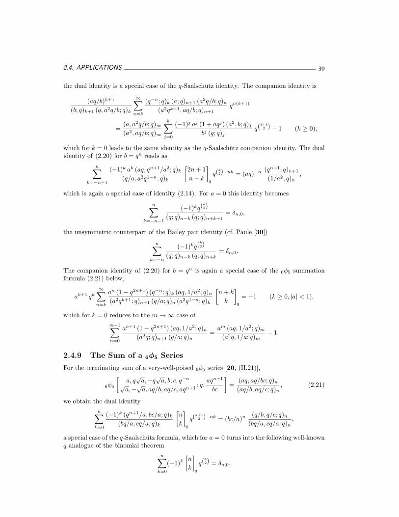
2.4. APPLICATIONS 39
the dual identity is a special case of the q-Saalschutz identity. The companion identity is
(aq/b)k+1
(b; q)k+1 (q, a2q/b; q)k
∞∑
n=k
(q−n; q)k (a; q)n+1 (a2q/b; q)n
(a2qk+1, aq/b; q)n+1qn(k+1)
=(a, a2q/b; q)∞(a2, aq/b; q)∞
k∑
j=0
(−1)j aj (1 + aqj) (a2, b; q)j
bj (q; q)jq(
j+12 ) − 1 (k ≥ 0),
which for k = 0 leads to the same identity as the q-Saalschutz companion identity. The dualidentity of (2.20) for b = qn reads as
n∑
k=−n−1
(−1)k ak (aq, qn+1/a2; q)k
(q/a, a2q1−n; q)k
[2n + 1n− k
]
q
q(k2)−nk = (aq)−n (qn+1; q)n+1
(1/a2; q)n,
which is again a special case of identity (2.14). For a = 0 this identity becomes
n∑
k=−n−1
(−1)kq(k2)
(q; q)n−k (q; q)n+k+1= δn,0,
the unsymmetric counterpart of the Bailey pair identity (cf. Paule [30])
n∑
k=−n
(−1)kq(k2)
(q; q)n−k (q; q)n+k= δn,0.
The companion identity of (2.20) for b = qn is again a special case of the 6φ5 summationformula (2.21) below,
ak+1 qk∞∑
n=k
an (1− q2n+1) (q−n; q)k (aq, 1/a2; q)n
(a2qk+1; q)n+1 (q/a; q)n (a2q1−n; q)k
[n + k
k
]
q
= −1 (k ≥ 0, |a| < 1),
which for k = 0 reduces to the m →∞ case ofm−1∑n=0
an+1 (1− q2n+1) (aq, 1/a2; q)n
(a2q; q)n+1 (q/a; q)n=
am (aq, 1/a2; q)m
(a2q, 1/a; q)m− 1.
2.4.9 The Sum of a 6φ5 Series
For the terminating sum of a very-well-poised 6φ5 series [20, (II.21)],
6φ5
[a, q
√a,−q
√a, b, c, q−n
√a,−√a, aq/b, aq/c, aqn+1
; q,aqn+1
bc
]=
(aq, aq/bc; q)n
(aq/b, aq/c; q)n, (2.21)
we obtain the dual identityn∑
k=0
(−1)k (qn+1/a, bc/a; q)k
(bq/a, cq/a; q)k
[n
k
]
q
q(k+12 )−nk = (bc/a)n (q/b, q/c; q)n
(bq/a, cq/a; q)n,
a special case of the q-Saalschutz formula, which for a = 0 turns into the following well-knownq-analogue of the binomial theorem
n∑
k=0
(−1)k
[n
k
]
q
q(k2) = δn,0.
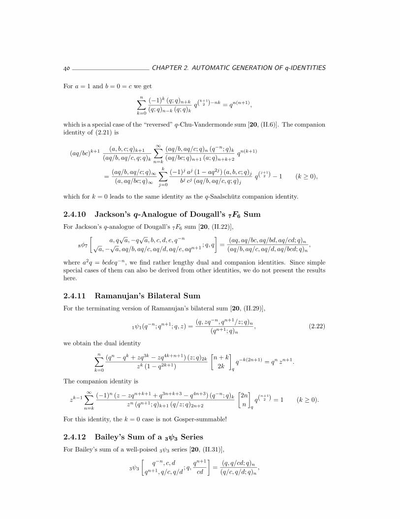
40 CHAPTER 2. AUTOMATIC GENERATION OF q-IDENTITIES
For a = 1 and b = 0 = c we get
n∑
k=0
(−1)k (q; q)n+k
(q; q)n−k (q; q)kq(
k+12 )−nk = qn(n+1),
which is a special case of the “reversed” q-Chu-Vandermonde sum [20, (II.6)]. The companionidentity of (2.21) is
(aq/bc)k+1 (a, b, c; q)k+1
(aq/b, aq/c, q; q)k
∞∑
n=k
(aq/b, aq/c; q)n (q−n; q)k
(aq/bc; q)n+1 (a; q)n+k+2qn(k+1)
=(aq/b, aq/c; q)∞(a, aq/bc; q)∞
k∑
j=0
(−1)j aj (1− aq2j) (a, b, c; q)j
bj cj (aq/b, aq/c, q; q)jq(
j+12 ) − 1 (k ≥ 0),
which for k = 0 leads to the same identity as the q-Saalschutz companion identity.
2.4.10 Jackson’s q-Analogue of Dougall’s 7F6 Sum
For Jackson’s q-analogue of Dougall’s 7F6 sum [20, (II.22)],
8φ7
[a, q
√a,−q
√a, b, c, d, e, q−n
√a,−√a, aq/b, aq/c, aq/d, aq/e, aqn+1
; q, q]
=(aq, aq/bc, aq/bd, aq/cd; q)n
(aq/b, aq/c, aq/d, aq/bcd; q)n,
where a2q = bcdeq−n, we find rather lengthy dual and companion identities. Since simplespecial cases of them can also be derived from other identities, we do not present the resultshere.
2.4.11 Ramanujan’s Bilateral Sum
For the terminating version of Ramanujan’s bilateral sum [20, (II.29)],
1ψ1(q−n; qn+1; q, z) =(q, zq−n, qn+1/z; q)n
(qn+1; q)n, (2.22)
we obtain the dual identity
n∑
k=0
(qn − qk + zq3k − zq4k+n+1) (z; q)2k
zk (1− q2k+1)
[n + k
2k
]
q
q−k(2n+1) = qn zn+1.
The companion identity is
zk−1∞∑
n=k
(−1)n (z − zqn+k+1 + q3n+k+3 − q4n+3) (q−n; q)k
zn (qn+1; q)k+1 (q/z; q)2n+2
[2n
n
]
q
q(n+1
2 ) = 1 (k ≥ 0).
For this identity, the k = 0 case is not Gosper-summable!
2.4.12 Bailey’s Sum of a 3ψ3 Series
For Bailey’s sum of a well-poised 3ψ3 series [20, (II.31)],
3ψ3
[q−n, c, d
qn+1, q/c, q/d; q,
qn+1
cd
]=
(q, q/cd; q)n
(q/c, q/d; q)n,
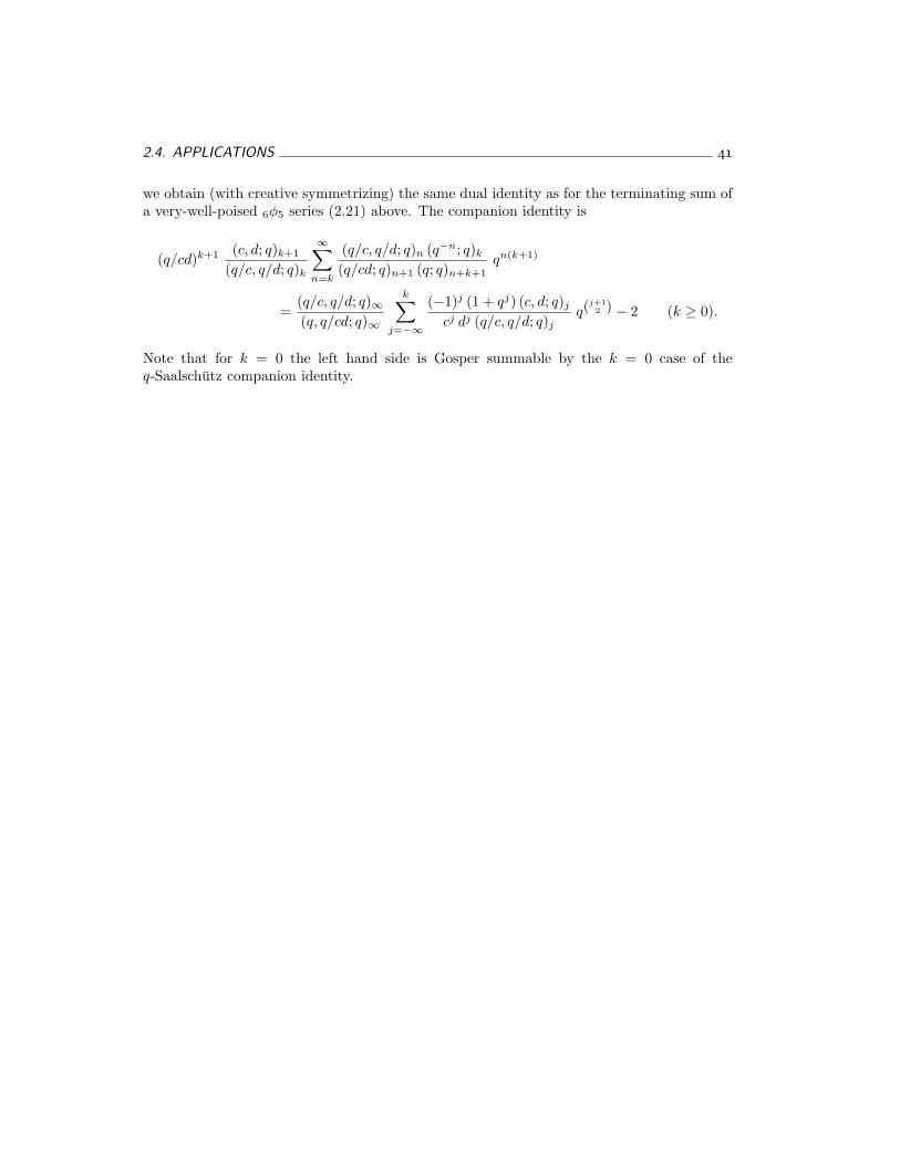
2.4. APPLICATIONS 41
we obtain (with creative symmetrizing) the same dual identity as for the terminating sum ofa very-well-poised 6φ5 series (2.21) above. The companion identity is
(q/cd)k+1 (c, d; q)k+1
(q/c, q/d; q)k
∞∑
n=k
(q/c, q/d; q)n (q−n; q)k
(q/cd; q)n+1 (q; q)n+k+1qn(k+1)
=(q/c, q/d; q)∞(q, q/cd; q)∞
k∑
j=−∞
(−1)j (1 + qj) (c, d; q)j
cj dj (q/c, q/d; q)jq(
j+12 ) − 2 (k ≥ 0).
Note that for k = 0 the left hand side is Gosper summable by the k = 0 case of theq-Saalschutz companion identity.

42
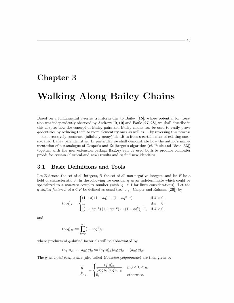
43
Chapter 3
Walking Along Bailey Chains
Based on a fundamental q-series transform due to Bailey [15], whose potential for itera-tion was independently observed by Andrews [9,10] and Paule [27,28], we shall describe inthis chapter how the concept of Bailey pairs and Bailey chains can be used to easily proveq-identities by reducing them to more elementary ones as well as — by reversing this process— to successively construct (infinitely many) identities from a certain class of existing ones,so-called Bailey pair identities. In particular we shall demonstrate how the author’s imple-mentation of a q-analogue of Gosper’s and Zeilberger’s algorithm (cf. Paule and Riese [33])together with the new extension package Bailey can be used both to produce computerproofs for certain (classical and new) results and to find new identities.
3.1 Basic Definitions and Tools
Let Z denote the set of all integers, N the set of all non-negative integers, and let F be afield of characteristic 0. In the following we consider q as an indeterminate which could bespecialized to a non-zero complex number (with |q| < 1 for limit considerations). Let theq-shifted factorial of a ∈ F be defined as usual (see, e.g., Gasper and Rahman [20]) by
(a; q)k :=
(1− a) (1− aq) · · · (1− aqk−1), if k > 0,1, if k = 0,[(1− aq−1) (1− aq−2) · · · (1− aqk)
]−1, if k < 0,
and
(a; q)∞ :=∞∏
k=0
(1− aqk),
where products of q-shifted factorials will be abbreviated by
(a1, a2, . . . , am; q)k := (a1; q)k (a2; q)k · · · (am; q)k.
The q-binomial coefficients (also called Gaussian polynomials) are then given by
[n
k
]
q
:=
(q; q)n
(q; q)k (q; q)n−k, if 0 ≤ k ≤ n,
0, otherwise.
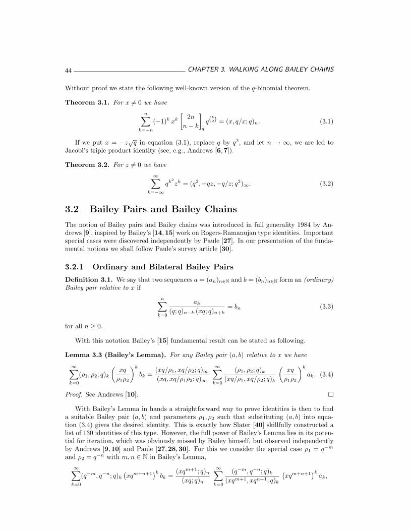
44 CHAPTER 3. WALKING ALONG BAILEY CHAINS
Without proof we state the following well-known version of the q-binomial theorem.
Theorem 3.1. For x 6= 0 we have
n∑
k=−n
(−1)k xk
[2n
n− k
]
q
q(k2) = (x, q/x; q)n. (3.1)
If we put x = −z√
q in equation (3.1), replace q by q2, and let n → ∞, we are led toJacobi’s triple product identity (see, e.g., Andrews [6,7]).
Theorem 3.2. For z 6= 0 we have
∞∑
k=−∞qk2
zk = (q2,−qz,−q/z; q2)∞. (3.2)
3.2 Bailey Pairs and Bailey Chains
The notion of Bailey pairs and Bailey chains was introduced in full generality 1984 by An-drews [9], inspired by Bailey’s [14,15] work on Rogers-Ramanujan type identities. Importantspecial cases were discovered independently by Paule [27]. In our presentation of the funda-mental notions we shall follow Paule’s survey article [30].
3.2.1 Ordinary and Bilateral Bailey Pairs
Definition 3.1. We say that two sequences a = (an)n∈N and b = (bn)n∈N form an (ordinary)Bailey pair relative to x if
n∑
k=0
ak
(q; q)n−k (xq; q)n+k= bn (3.3)
for all n ≥ 0.
With this notation Bailey’s [15] fundamental result can be stated as following.
Lemma 3.3 (Bailey’s Lemma). For any Bailey pair (a, b) relative to x we have
∞∑
k=0
(ρ1, ρ2; q)k
(xq
ρ1ρ2
)k
bk =(xq/ρ1, xq/ρ2; q)∞(xq, xq/ρ1ρ2; q)∞
∞∑
k=0
(ρ1, ρ2; q)k
(xq/ρ1, xq/ρ2; q)k
(xq
ρ1ρ2
)k
ak. (3.4)
Proof. See Andrews [10].
With Bailey’s Lemma in hands a straightforward way to prove identities is then to finda suitable Bailey pair (a, b) and parameters ρ1, ρ2 such that substituting (a, b) into equa-tion (3.4) gives the desired identity. This is exactly how Slater [40] skillfully constructed alist of 130 identities of this type. However, the full power of Bailey’s Lemma lies in its poten-tial for iteration, which was obviously missed by Bailey himself, but observed independentlyby Andrews [9,10] and Paule [27,28,30]. For this we consider the special case ρ1 = q−m
and ρ2 = q−n with m,n ∈ N in Bailey’s Lemma,
∞∑
k=0
(q−m, q−n; q)k
(xqm+n+1
)kbk =
(xqm+1; q)n
(xq; q)n
∞∑
k=0
(q−m, q−n; q)k
(xqm+1, xqn+1; q)k
(xqm+n+1
)kak,
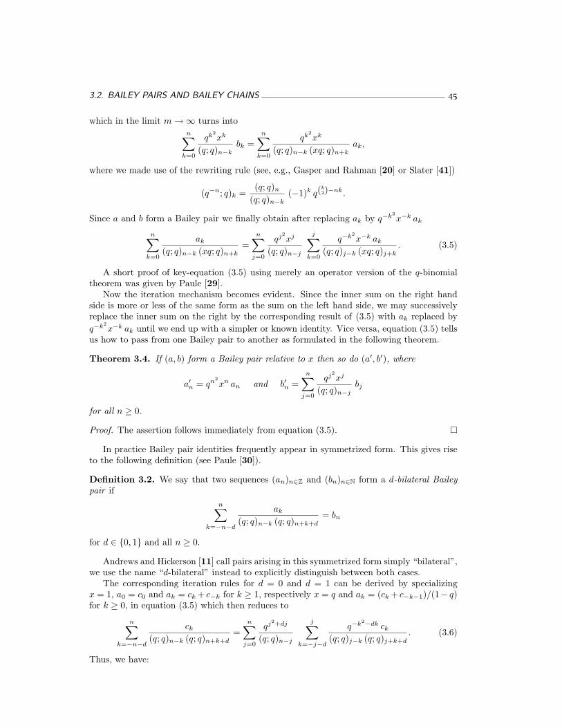
3.2. BAILEY PAIRS AND BAILEY CHAINS 45
which in the limit m →∞ turns inton∑
k=0
qk2xk
(q; q)n−kbk =
n∑
k=0
qk2xk
(q; q)n−k (xq; q)n+kak,
where we made use of the rewriting rule (see, e.g., Gasper and Rahman [20] or Slater [41])
(q−n; q)k =(q; q)n
(q; q)n−k(−1)k q(
k2)−nk.
Since a and b form a Bailey pair we finally obtain after replacing ak by q−k2x−k ak
n∑
k=0
ak
(q; q)n−k (xq; q)n+k=
n∑
j=0
qj2xj
(q; q)n−j
j∑
k=0
q−k2x−k ak
(q; q)j−k (xq; q)j+k. (3.5)
A short proof of key-equation (3.5) using merely an operator version of the q-binomialtheorem was given by Paule [29].
Now the iteration mechanism becomes evident. Since the inner sum on the right handside is more or less of the same form as the sum on the left hand side, we may successivelyreplace the inner sum on the right by the corresponding result of (3.5) with ak replaced byq−k2
x−k ak until we end up with a simpler or known identity. Vice versa, equation (3.5) tellsus how to pass from one Bailey pair to another as formulated in the following theorem.
Theorem 3.4. If (a, b) form a Bailey pair relative to x then so do (a′, b′), where
a′n = qn2xn an and b′n =
n∑
j=0
qj2xj
(q; q)n−jbj
for all n ≥ 0.
Proof. The assertion follows immediately from equation (3.5).
In practice Bailey pair identities frequently appear in symmetrized form. This gives riseto the following definition (see Paule [30]).
Definition 3.2. We say that two sequences (an)n∈Z and (bn)n∈N form a d-bilateral Baileypair if
n∑
k=−n−d
ak
(q; q)n−k (q; q)n+k+d= bn
for d ∈ {0, 1} and all n ≥ 0.
Andrews and Hickerson [11] call pairs arising in this symmetrized form simply “bilateral”,we use the name “d-bilateral” instead to explicitly distinguish between both cases.
The corresponding iteration rules for d = 0 and d = 1 can be derived by specializingx = 1, a0 = c0 and ak = ck + c−k for k ≥ 1, respectively x = q and ak = (ck + c−k−1)/(1− q)for k ≥ 0, in equation (3.5) which then reduces to
n∑
k=−n−d
ck
(q; q)n−k (q; q)n+k+d=
n∑
j=0
qj2+dj
(q; q)n−j
j∑
k=−j−d
q−k2−dk ck
(q; q)j−k (q; q)j+k+d. (3.6)
Thus, we have:
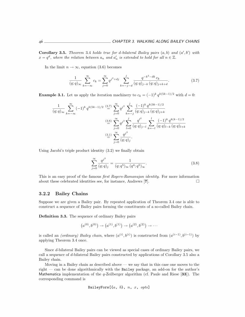
46 CHAPTER 3. WALKING ALONG BAILEY CHAINS
Corollary 3.5. Theorem 3.4 holds true for d-bilateral Bailey pairs (a, b) and (a′, b′) withx = qd, where the relation between an and a′n is extended to hold for all n ∈ Z.
In the limit n →∞, equation (3.6) becomes
1(q; q)∞
∞∑
k=−∞ck =
∞∑
j=0
qj2+dj
j∑
k=−j−d
q−k2−dk ck
(q; q)j−k (q; q)j+k+d. (3.7)
Example 3.1. Let us apply the iteration machinery to ck = (−1)k qk(5k−1)/2 with d = 0:
1(q; q)∞
∞∑
k=−∞(−1)k qk(5k−1)/2 (3.7)
=∞∑
j=0
qj2j∑
k=−j
(−1)k qk(3k−1)/2
(q; q)j−k (q; q)j+k
(3.6)=
∞∑
j=0
qj2j∑
l=0
ql2
(q; q)j−l
l∑
k=−l
(−1)k qk(k−1)/2
(q; q)l−k (q; q)l+k
(3.1)=
∞∑
j=0
qj2
(q; q)j.
Using Jacobi’s triple product identity (3.2) we finally obtain
∞∑
j=0
qj2
(q; q)j=
1(q; q5)∞ (q4; q5)∞
. (3.8)
This is an easy proof of the famous first Rogers-Ramanujan identity. For more informationabout these celebrated identities see, for instance, Andrews [7].
3.2.2 Bailey Chains
Suppose we are given a Bailey pair. By repeated application of Theorem 3.4 one is able toconstruct a sequence of Bailey pairs forming the constituents of a so-called Bailey chain.
Definition 3.3. The sequence of ordinary Bailey pairs
(a(0), b(0)
) → (a(1), b(1)
) → (a(2), b(2)
) → · · ·
is called an (ordinary) Bailey chain, where (a(i), b(i)) is constructed from (a(i−1), b(i−1)) byapplying Theorem 3.4 once.
Since d-bilateral Bailey pairs can be viewed as special cases of ordinary Bailey pairs, wecall a sequence of d-bilateral Bailey pairs constructed by applications of Corollary 3.5 also aBailey chain.
Moving in a Bailey chain as described above — we say that in this case one moves to theright — can be done algorithmically with the Bailey package, an add-on for the author’sMathematica implementation of the q-Zeilberger algorithm (cf. Paule and Riese [33]). Thecorresponding command is
BaileyForw[{a, b}, n, x, opts]
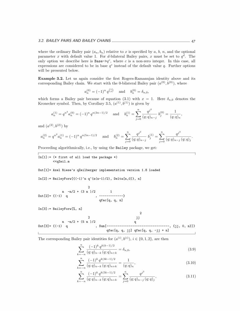
3.2. BAILEY PAIRS AND BAILEY CHAINS 47
where the ordinary Bailey pair (an, bn) relative to x is specified by a, b, n, and the optionalparameter x with default value 1. For d-bilateral Bailey pairs, x must be set to qd. Theonly option we describe here is Base->qc, where c is a non-zero integer. In this case, allexpressions are considered to be in base qc instead of the default value q. Further optionswill be presented below.
Example 3.2. Let us again consider the first Rogers-Ramanujan identity above and itscorresponding Bailey chain. We start with the 0-bilateral Bailey pair (a(0), b(0)), where
a(0)n = (−1)n q(
n2) and b(0)
n = δn,0,
which forms a Bailey pair because of equation (3.1) with x = 1. Here δn,0 denotes theKronecker symbol. Then, by Corollary 3.5, (a(1), b(1)) is given by
a(1)n = qn2
a(0)n = (−1)n qn(3n−1)/2 and b(1)
n =n∑
j=0
qj2
(q; q)n−jb(0)j =
1(q; q)n
,
and (a(2), b(2)) by
a(2)n = qn2
a(1)n = (−1)n qn(5n−1)/2 and b(2)
n =n∑
j=0
qj2
(q; q)n−jb(1)j =
n∑
j=0
qj2
(q; q)n−j (q; q)j.
Proceeding algorithmically, i.e., by using the Bailey package, we get:
In[1]:= (* first of all load the package *)
<<qZeil.m
Out[1]= Axel Riese’s qZeilberger implementation version 1.8 loaded
In[2]:= BaileyForw[{(-1)^n q^(n(n-1)/2), Delta[n,0]}, n]
2
n -n/2 + (3 n )/2 1
Out[2]= {(-1) q , -------------}
qfac[q, q, n]
In[3]:= BaileyForw[%, n]
2
2 jj
n -n/2 + (5 n )/2 q
Out[3]= {(-1) q , Sum[----------------------------------, {jj, 0, n}]}
qfac[q, q, jj] qfac[q, q, -jj + n]
The corresponding Bailey pair identities for (a(i), b(i)), i ∈ {0, 1, 2}, are thenn∑
k=−n
(−1)k qk(k−1)/2
(q; q)n−k (q; q)n+k= δn,0, (3.9)
n∑
k=−n
(−1)k qk(3k−1)/2
(q; q)n−k (q; q)n+k=
1(q; q)n
, (3.10)
n∑
k=−n
(−1)k qk(5k−1)/2
(q; q)n−k (q; q)n+k=
n∑
j=0
qj2
(q; q)n−j (q; q)j, (3.11)
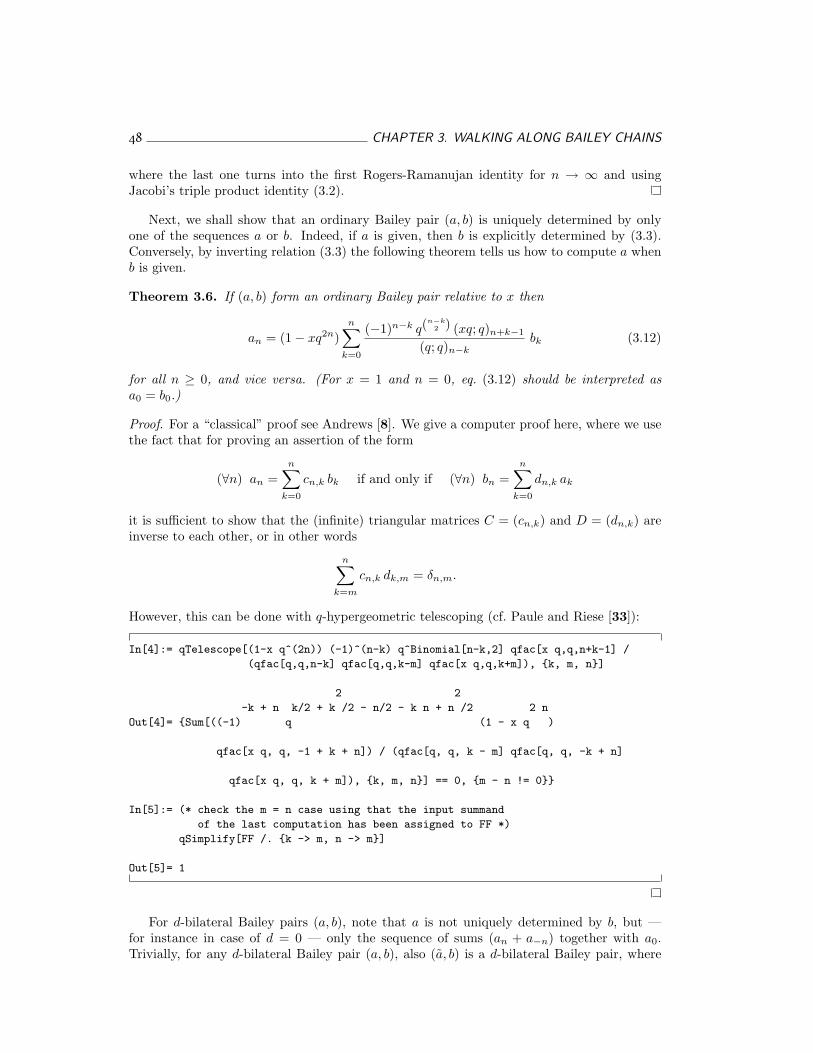
48 CHAPTER 3. WALKING ALONG BAILEY CHAINS
where the last one turns into the first Rogers-Ramanujan identity for n → ∞ and usingJacobi’s triple product identity (3.2).
Next, we shall show that an ordinary Bailey pair (a, b) is uniquely determined by onlyone of the sequences a or b. Indeed, if a is given, then b is explicitly determined by (3.3).Conversely, by inverting relation (3.3) the following theorem tells us how to compute a whenb is given.
Theorem 3.6. If (a, b) form an ordinary Bailey pair relative to x then
an = (1− xq2n)n∑
k=0
(−1)n−k q(n−k
2 ) (xq; q)n+k−1
(q; q)n−kbk (3.12)
for all n ≥ 0, and vice versa. (For x = 1 and n = 0, eq. (3.12) should be interpreted asa0 = b0.)
Proof. For a “classical” proof see Andrews [8]. We give a computer proof here, where we usethe fact that for proving an assertion of the form
(∀n) an =n∑
k=0
cn,k bk if and only if (∀n) bn =n∑
k=0
dn,k ak
it is sufficient to show that the (infinite) triangular matrices C = (cn,k) and D = (dn,k) areinverse to each other, or in other words
n∑
k=m
cn,k dk,m = δn,m.
However, this can be done with q-hypergeometric telescoping (cf. Paule and Riese [33]):
In[4]:= qTelescope[(1-x q^(2n)) (-1)^(n-k) q^Binomial[n-k,2] qfac[x q,q,n+k-1] /
(qfac[q,q,n-k] qfac[q,q,k-m] qfac[x q,q,k+m]), {k, m, n}]
2 2
-k + n k/2 + k /2 - n/2 - k n + n /2 2 n
Out[4]= {Sum[((-1) q (1 - x q )
qfac[x q, q, -1 + k + n]) / (qfac[q, q, k - m] qfac[q, q, -k + n]
qfac[x q, q, k + m]), {k, m, n}] == 0, {m - n != 0}}
In[5]:= (* check the m = n case using that the input summand
of the last computation has been assigned to FF *)
qSimplify[FF /. {k -> m, n -> m}]
Out[5]= 1
For d-bilateral Bailey pairs (a, b), note that a is not uniquely determined by b, but —for instance in case of d = 0 — only the sequence of sums (an + a−n) together with a0.Trivially, for any d-bilateral Bailey pair (a, b), also (a, b) is a d-bilateral Bailey pair, where
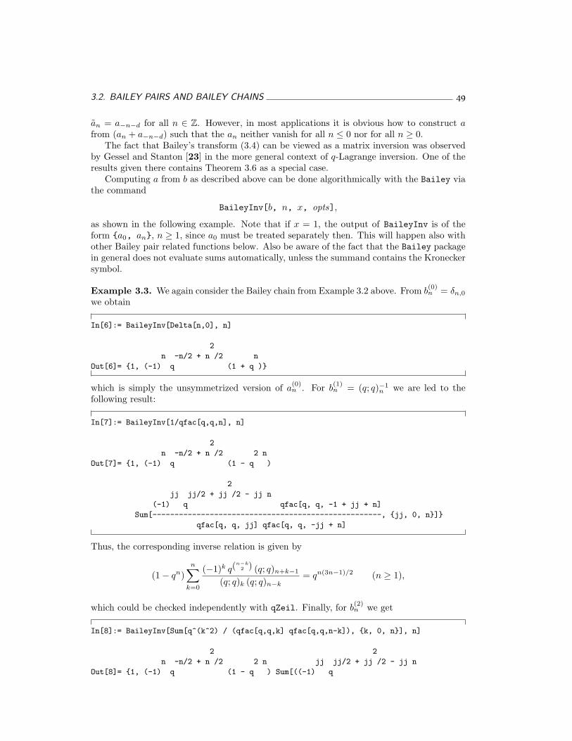
3.2. BAILEY PAIRS AND BAILEY CHAINS 49
an = a−n−d for all n ∈ Z. However, in most applications it is obvious how to construct afrom (an + a−n−d) such that the an neither vanish for all n ≤ 0 nor for all n ≥ 0.
The fact that Bailey’s transform (3.4) can be viewed as a matrix inversion was observedby Gessel and Stanton [23] in the more general context of q-Lagrange inversion. One of theresults given there contains Theorem 3.6 as a special case.
Computing a from b as described above can be done algorithmically with the Bailey viathe command
BaileyInv[b, n, x, opts],
as shown in the following example. Note that if x = 1, the output of BaileyInv is of theform {a0, an}, n ≥ 1, since a0 must be treated separately then. This will happen also withother Bailey pair related functions below. Also be aware of the fact that the Bailey packagein general does not evaluate sums automatically, unless the summand contains the Kroneckersymbol.
Example 3.3. We again consider the Bailey chain from Example 3.2 above. From b(0)n = δn,0
we obtain
In[6]:= BaileyInv[Delta[n,0], n]
2
n -n/2 + n /2 n
Out[6]= {1, (-1) q (1 + q )}
which is simply the unsymmetrized version of a(0)n . For b
(1)n = (q; q)−1
n we are led to thefollowing result:
In[7]:= BaileyInv[1/qfac[q,q,n], n]
2
n -n/2 + n /2 2 n
Out[7]= {1, (-1) q (1 - q )
2
jj jj/2 + jj /2 - jj n
(-1) q qfac[q, q, -1 + jj + n]
Sum[----------------------------------------------------, {jj, 0, n}]}
qfac[q, q, jj] qfac[q, q, -jj + n]
Thus, the corresponding inverse relation is given by
(1− qn)n∑
k=0
(−1)k q(n−k
2 ) (q; q)n+k−1
(q; q)k (q; q)n−k= qn(3n−1)/2 (n ≥ 1),
which could be checked independently with qZeil. Finally, for b(2)n we get
In[8]:= BaileyInv[Sum[q^(k^2) / (qfac[q,q,k] qfac[q,q,n-k]), {k, 0, n}], n]
2 2
n -n/2 + n /2 2 n jj jj/2 + jj /2 - jj n
Out[8]= {1, (-1) q (1 - q ) Sum[((-1) q
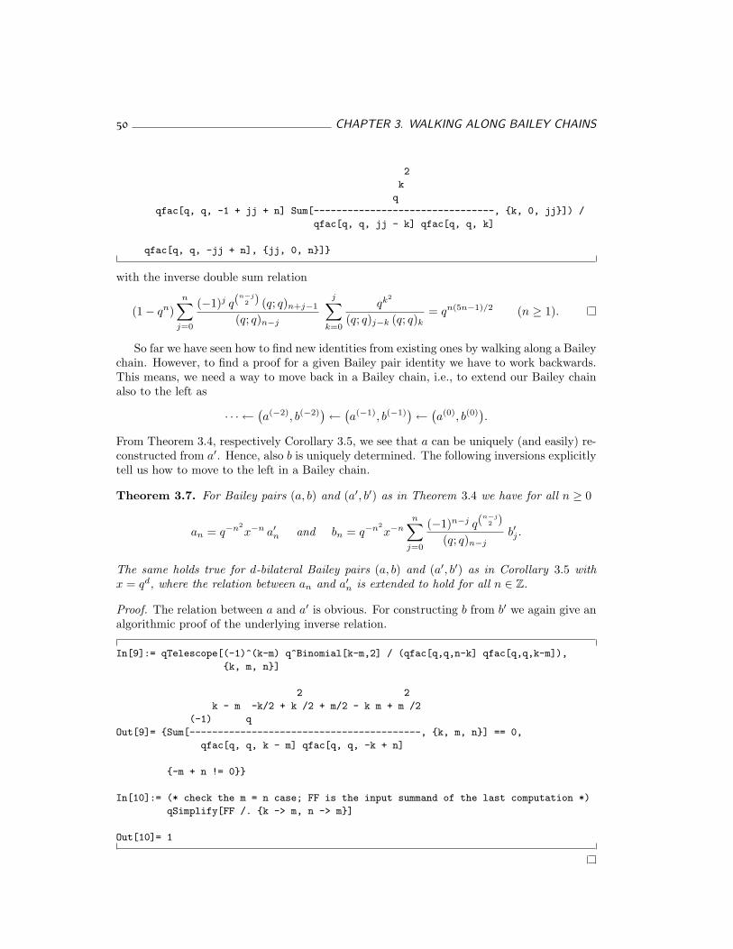
50 CHAPTER 3. WALKING ALONG BAILEY CHAINS
2
k
q
qfac[q, q, -1 + jj + n] Sum[--------------------------------, {k, 0, jj}]) /
qfac[q, q, jj - k] qfac[q, q, k]
qfac[q, q, -jj + n], {jj, 0, n}]}
with the inverse double sum relation
(1− qn)n∑
j=0
(−1)j q(n−j
2 ) (q; q)n+j−1
(q; q)n−j
j∑
k=0
qk2
(q; q)j−k (q; q)k= qn(5n−1)/2 (n ≥ 1).
So far we have seen how to find new identities from existing ones by walking along a Baileychain. However, to find a proof for a given Bailey pair identity we have to work backwards.This means, we need a way to move back in a Bailey chain, i.e., to extend our Bailey chainalso to the left as
· · · ← (a(−2), b(−2)
) ← (a(−1), b(−1)
) ← (a(0), b(0)
).
From Theorem 3.4, respectively Corollary 3.5, we see that a can be uniquely (and easily) re-constructed from a′. Hence, also b is uniquely determined. The following inversions explicitlytell us how to move to the left in a Bailey chain.
Theorem 3.7. For Bailey pairs (a, b) and (a′, b′) as in Theorem 3.4 we have for all n ≥ 0
an = q−n2x−n a′n and bn = q−n2
x−nn∑
j=0
(−1)n−j q(n−j
2 )
(q; q)n−jb′j .
The same holds true for d-bilateral Bailey pairs (a, b) and (a′, b′) as in Corollary 3.5 withx = qd, where the relation between an and a′n is extended to hold for all n ∈ Z.
Proof. The relation between a and a′ is obvious. For constructing b from b′ we again give analgorithmic proof of the underlying inverse relation.
In[9]:= qTelescope[(-1)^(k-m) q^Binomial[k-m,2] / (qfac[q,q,n-k] qfac[q,q,k-m]),
{k, m, n}]
2 2
k - m -k/2 + k /2 + m/2 - k m + m /2
(-1) q
Out[9]= {Sum[-----------------------------------------, {k, m, n}] == 0,
qfac[q, q, k - m] qfac[q, q, -k + n]
{-m + n != 0}}
In[10]:= (* check the m = n case; FF is the input summand of the last computation *)
qSimplify[FF /. {k -> m, n -> m}]
Out[10]= 1
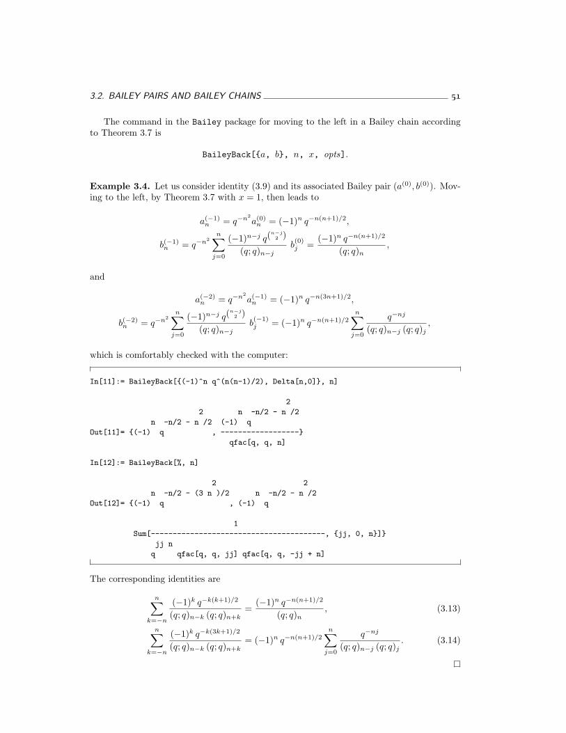
3.2. BAILEY PAIRS AND BAILEY CHAINS 51
The command in the Bailey package for moving to the left in a Bailey chain accordingto Theorem 3.7 is
BaileyBack[{a, b}, n, x, opts].
Example 3.4. Let us consider identity (3.9) and its associated Bailey pair (a(0), b(0)). Mov-ing to the left, by Theorem 3.7 with x = 1, then leads to
a(−1)n = q−n2
a(0)n = (−1)n q−n(n+1)/2,
b(−1)n = q−n2
n∑
j=0
(−1)n−j q(n−j
2 )
(q; q)n−jb(0)j =
(−1)n q−n(n+1)/2
(q; q)n,
and
a(−2)n = q−n2
a(−1)n = (−1)n q−n(3n+1)/2,
b(−2)n = q−n2
n∑
j=0
(−1)n−j q(n−j
2 )
(q; q)n−jb(−1)j = (−1)n q−n(n+1)/2
n∑
j=0
q−nj
(q; q)n−j (q; q)j,
which is comfortably checked with the computer:
In[11]:= BaileyBack[{(-1)^n q^(n(n-1)/2), Delta[n,0]}, n]
2
2 n -n/2 - n /2
n -n/2 - n /2 (-1) q
Out[11]= {(-1) q , ------------------}
qfac[q, q, n]
In[12]:= BaileyBack[%, n]
2 2
n -n/2 - (3 n )/2 n -n/2 - n /2
Out[12]= {(-1) q , (-1) q
1
Sum[----------------------------------------, {jj, 0, n}]}
jj n
q qfac[q, q, jj] qfac[q, q, -jj + n]
The corresponding identities are
n∑
k=−n
(−1)k q−k(k+1)/2
(q; q)n−k (q; q)n+k=
(−1)n q−n(n+1)/2
(q; q)n, (3.13)
n∑
k=−n
(−1)k q−k(3k+1)/2
(q; q)n−k (q; q)n+k= (−1)n q−n(n+1)/2
n∑
j=0
q−nj
(q; q)n−j (q; q)j. (3.14)
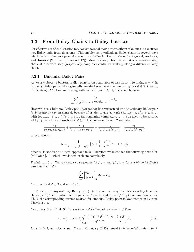
52 CHAPTER 3. WALKING ALONG BAILEY CHAINS
3.3 From Bailey Chains to Bailey Lattices
For effective use of our iteration mechanism we shall now present other techniques to constructnew Bailey pairs from given ones. This enables us to walk along Bailey chains in several wayswhich leads to the more general concept of a Bailey lattice introduced by Agarwal, Andrews,and Bressoud [2] (cf. also Bressoud [17]). More precisely, this means that one leaves a Baileychain at a certain step (respectively pair) and continues walking along a different Baileychain.
3.3.1 Binomial Bailey Pairs
As we saw above, d-bilateral Bailey pairs correspond more or less directly to taking x = qd inordinary Bailey pairs. More generally, we shall now treat the case x = qd for d ∈ N. Clearly,for arbitrary d ∈ N we are dealing with sums of (2n + d + 1) terms of the form
n∑
k=−n−d
ck
(q; q)n−k (q; q)n+k+d= bn.
However, the d-bilateral Bailey pair (c, b) cannot be transformed into an ordinary Bailey pair(a, b) relative to qd in general, because after identifying an with (c−n−d + cn)/(q; q)d, an−1
with (c−n−d+1 + cn−1)/(q; q)d, etc., the remaining terms c0, c−1, . . . , c−d need to be coveredall by a0, which is impossible for d ≥ 2. For instance, for d = 2 we obtain
c0
(q; q)n (q; q)n+2+
c−1
(q; q)n+1 (q; q)n+1+
c−2
(q; q)n+2 (q; q)n=
a0
(q; q)n (q3; q)n,
or equivalently
a0 =1
(1− q)(1− q2)
(c0 +
1− qn+2
1− qn+1c−1 + c−2
).
Since a0 is not free of n, this approach fails. Therefore we introduce the following definition(cf. Paule [30]) which avoids this problem completely.
Definition 3.4. We say that two sequences (An)n∈N and (Bn)n∈N form a binomial Baileypair relative to d if
n∑
k=0
[2n + d
n− k
]
q
Ak = Bn
for some fixed d ∈ N and all n ≥ 0.
Trivially, for any ordinary Bailey pair (a, b) relative to x = qd the corresponding binomialBailey pair (A, B) relative to d is given by An = an and Bn = (qd+1; q)2n bn, and vice versa.Thus, the corresponding inverse relation for binomial Bailey pairs follows immediately fromTheorem 3.6.
Corollary 3.8. If (A,B) form a binomial Bailey pair relative to d then
An = (1− q2n+d)n∑
k=0
(−1)n−k q(n−k
2 )
1− qn+k+d
[n + k + d
n− k
]
q
Bk (3.15)
for all n ≥ 0, and vice versa. (For n = 0 = d, eq. (3.15) should be interpreted as A0 = B0.)
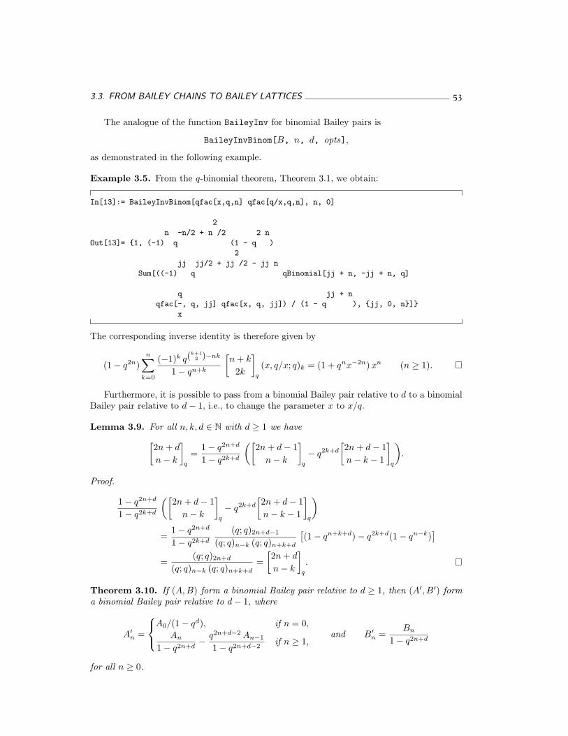
3.3. FROM BAILEY CHAINS TO BAILEY LATTICES 53
The analogue of the function BaileyInv for binomial Bailey pairs is
BaileyInvBinom[B, n, d, opts],
as demonstrated in the following example.
Example 3.5. From the q-binomial theorem, Theorem 3.1, we obtain:
In[13]:= BaileyInvBinom[qfac[x,q,n] qfac[q/x,q,n], n, 0]
2
n -n/2 + n /2 2 n
Out[13]= {1, (-1) q (1 - q )
2
jj jj/2 + jj /2 - jj n
Sum[((-1) q qBinomial[jj + n, -jj + n, q]
q jj + n
qfac[-, q, jj] qfac[x, q, jj]) / (1 - q ), {jj, 0, n}]}
x
The corresponding inverse identity is therefore given by
(1− q2n)n∑
k=0
(−1)k q(k+12 )−nk
1− qn+k
[n + k
2k
]
q
(x, q/x; q)k = (1 + qnx−2n)xn (n ≥ 1).
Furthermore, it is possible to pass from a binomial Bailey pair relative to d to a binomialBailey pair relative to d− 1, i.e., to change the parameter x to x/q.
Lemma 3.9. For all n, k, d ∈ N with d ≥ 1 we have[2n + d
n− k
]
q
=1− q2n+d
1− q2k+d
([2n + d− 1
n− k
]
q
− q2k+d
[2n + d− 1n− k − 1
]
q
).
Proof.
1− q2n+d
1− q2k+d
([2n + d− 1
n− k
]
q
− q2k+d
[2n + d− 1n− k − 1
]
q
)
=1− q2n+d
1− q2k+d
(q; q)2n+d−1
(q; q)n−k (q; q)n+k+d
[(1− qn+k+d)− q2k+d(1− qn−k)
]
=(q; q)2n+d
(q; q)n−k (q; q)n+k+d=
[2n + d
n− k
]
q
.
Theorem 3.10. If (A,B) form a binomial Bailey pair relative to d ≥ 1, then (A′, B′) forma binomial Bailey pair relative to d− 1, where
A′n =
A0/(1− qd), if n = 0,
An
1− q2n+d− q2n+d−2 An−1
1− q2n+d−2if n ≥ 1,
and B′n =
Bn
1− q2n+d
for all n ≥ 0.
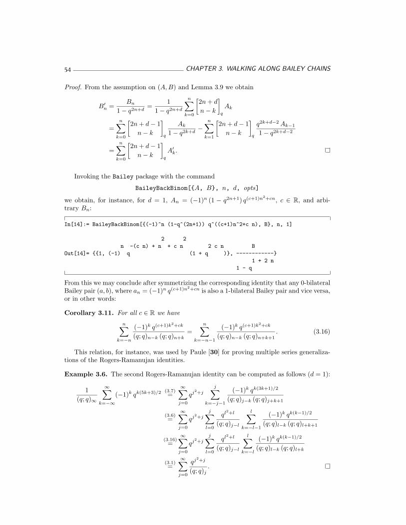
54 CHAPTER 3. WALKING ALONG BAILEY CHAINS
Proof. From the assumption on (A,B) and Lemma 3.9 we obtain
B′n =
Bn
1− q2n+d=
11− q2n+d
n∑
k=0
[2n + d
n− k
]
q
Ak
=n∑
k=0
[2n + d− 1
n− k
]
q
Ak
1− q2k+d−
n∑
k=1
[2n + d− 1
n− k
]
q
q2k+d−2 Ak−1
1− q2k+d−2
=n∑
k=0
[2n + d− 1
n− k
]
q
A′k.
Invoking the Bailey package with the command
BaileyBackBinom[{A, B}, n, d, opts]
we obtain, for instance, for d = 1, An = (−1)n (1 − q2n+1) q(c+1)n2+cn, c ∈ R, and arbi-trary Bn:
In[14]:= BaileyBackBinom[{(-1)^n (1-q^(2n+1)) q^((c+1)n^2+c n), B}, n, 1]
2 2
n -(c n) + n + c n 2 c n B
Out[14]= {{1, (-1) q (1 + q )}, ------------}
1 + 2 n
1 - q
From this we may conclude after symmetrizing the corresponding identity that any 0-bilateralBailey pair (a, b), where an = (−1)n q(c+1)n2+cn is also a 1-bilateral Bailey pair and vice versa,or in other words:
Corollary 3.11. For all c ∈ R we have
n∑
k=−n
(−1)k q(c+1)k2+ck
(q; q)n−k (q; q)n+k=
n∑
k=−n−1
(−1)k q(c+1)k2+ck
(q; q)n−k (q; q)n+k+1. (3.16)
This relation, for instance, was used by Paule [30] for proving multiple series generaliza-tions of the Rogers-Ramanujan identities.
Example 3.6. The second Rogers-Ramanujan identity can be computed as follows (d = 1):
1(q; q)∞
∞∑
k=−∞(−1)k qk(5k+3)/2 (3.7)
=∞∑
j=0
qj2+j
j∑
k=−j−1
(−1)k qk(3k+1)/2
(q; q)j−k (q; q)j+k+1
(3.6)=
∞∑
j=0
qj2+j
j∑
l=0
ql2+l
(q; q)j−l
l∑
k=−l−1
(−1)k qk(k−1)/2
(q; q)l−k (q; q)l+k+1
(3.16)=
∞∑
j=0
qj2+j
j∑
l=0
ql2+l
(q; q)j−l
l∑
k=−l
(−1)k qk(k−1)/2
(q; q)l−k (q; q)l+k
(3.1)=
∞∑
j=0
qj2+j
(q; q)j.
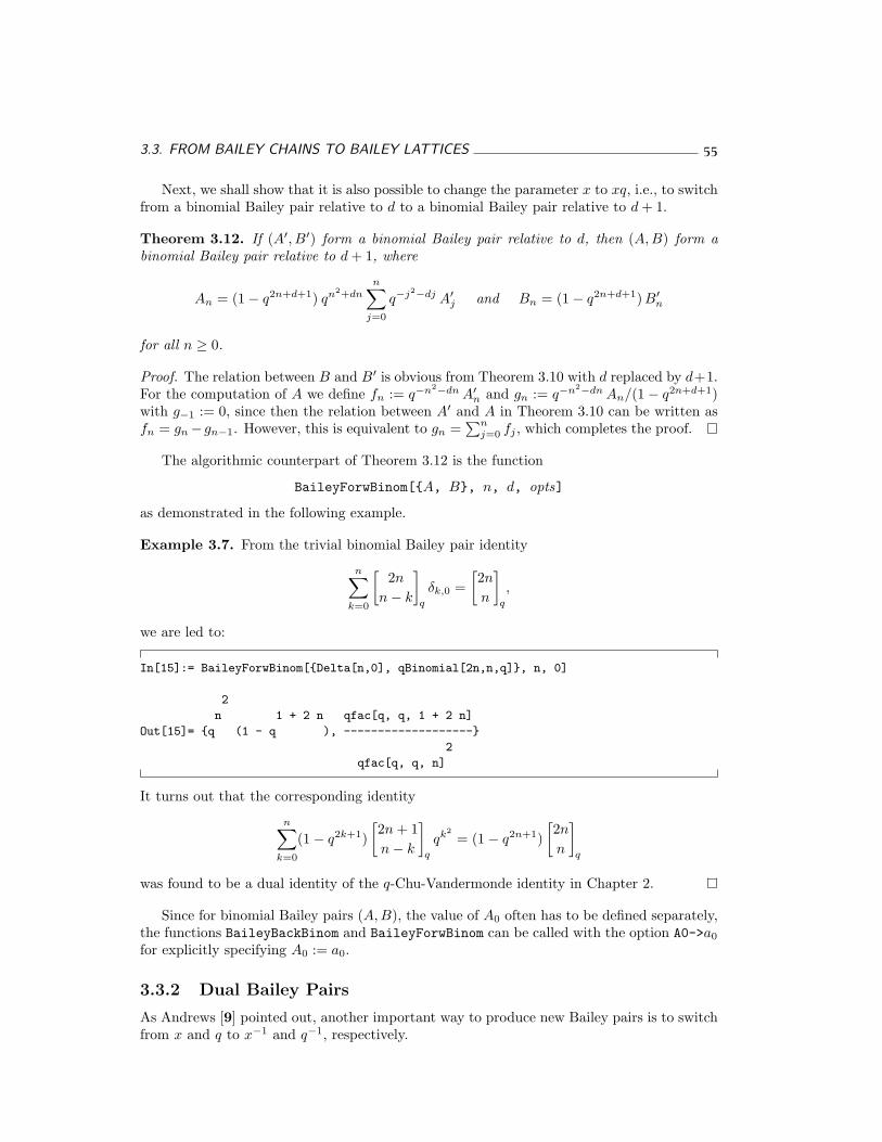
3.3. FROM BAILEY CHAINS TO BAILEY LATTICES 55
Next, we shall show that it is also possible to change the parameter x to xq, i.e., to switchfrom a binomial Bailey pair relative to d to a binomial Bailey pair relative to d + 1.
Theorem 3.12. If (A′, B′) form a binomial Bailey pair relative to d, then (A,B) form abinomial Bailey pair relative to d + 1, where
An = (1− q2n+d+1) qn2+dnn∑
j=0
q−j2−dj A′j and Bn = (1− q2n+d+1)B′n
for all n ≥ 0.
Proof. The relation between B and B′ is obvious from Theorem 3.10 with d replaced by d+1.For the computation of A we define fn := q−n2−dn A′n and gn := q−n2−dn An/(1− q2n+d+1)with g−1 := 0, since then the relation between A′ and A in Theorem 3.10 can be written asfn = gn− gn−1. However, this is equivalent to gn =
∑nj=0 fj , which completes the proof.
The algorithmic counterpart of Theorem 3.12 is the function
BaileyForwBinom[{A, B}, n, d, opts]
as demonstrated in the following example.
Example 3.7. From the trivial binomial Bailey pair identity
n∑
k=0
[2n
n− k
]
q
δk,0 =[2n
n
]
q
,
we are led to:
In[15]:= BaileyForwBinom[{Delta[n,0], qBinomial[2n,n,q]}, n, 0]
2
n 1 + 2 n qfac[q, q, 1 + 2 n]
Out[15]= {q (1 - q ), -------------------}
2
qfac[q, q, n]
It turns out that the corresponding identity
n∑
k=0
(1− q2k+1)[2n + 1n− k
]
q
qk2= (1− q2n+1)
[2n
n
]
q
was found to be a dual identity of the q-Chu-Vandermonde identity in Chapter 2.
Since for binomial Bailey pairs (A,B), the value of A0 often has to be defined separately,the functions BaileyBackBinom and BaileyForwBinom can be called with the option A0->a0
for explicitly specifying A0 := a0.
3.3.2 Dual Bailey Pairs
As Andrews [9] pointed out, another important way to produce new Bailey pairs is to switchfrom x and q to x−1 and q−1, respectively.
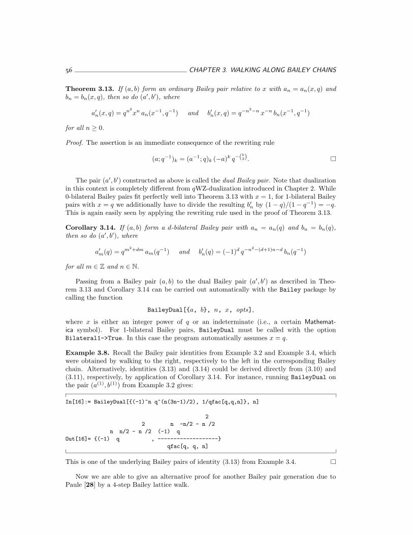
56 CHAPTER 3. WALKING ALONG BAILEY CHAINS
Theorem 3.13. If (a, b) form an ordinary Bailey pair relative to x with an = an(x, q) andbn = bn(x, q), then so do (a′, b′), where
a′n(x, q) = qn2xn an(x−1, q−1) and b′n(x, q) = q−n2−n x−n bn(x−1, q−1)
for all n ≥ 0.
Proof. The assertion is an immediate consequence of the rewriting rule
(a; q−1)k = (a−1; q)k (−a)k q−(k2).
The pair (a′, b′) constructed as above is called the dual Bailey pair. Note that dualizationin this context is completely different from qWZ-dualization introduced in Chapter 2. While0-bilateral Bailey pairs fit perfectly well into Theorem 3.13 with x = 1, for 1-bilateral Baileypairs with x = q we additionally have to divide the resulting b′n by (1− q)/(1− q−1) = −q.This is again easily seen by applying the rewriting rule used in the proof of Theorem 3.13.
Corollary 3.14. If (a, b) form a d-bilateral Bailey pair with an = an(q) and bn = bn(q),then so do (a′, b′), where
a′m(q) = qm2+dm am(q−1) and b′n(q) = (−1)d q−n2−(d+1)n−d bn(q−1)
for all m ∈ Z and n ∈ N.
Passing from a Bailey pair (a, b) to the dual Bailey pair (a′, b′) as described in Theo-rem 3.13 and Corollary 3.14 can be carried out automatically with the Bailey package bycalling the function
BaileyDual[{a, b}, n, x, opts],
where x is either an integer power of q or an indeterminate (i.e., a certain Mathemat-ica symbol). For 1-bilateral Bailey pairs, BaileyDual must be called with the optionBilateral1->True. In this case the program automatically assumes x = q.
Example 3.8. Recall the Bailey pair identities from Example 3.2 and Example 3.4, whichwere obtained by walking to the right, respectively to the left in the corresponding Baileychain. Alternatively, identities (3.13) and (3.14) could be derived directly from (3.10) and(3.11), respectively, by application of Corollary 3.14. For instance, running BaileyDual onthe pair (a(1), b(1)) from Example 3.2 gives:
In[16]:= BaileyDual[{(-1)^n q^(n(3n-1)/2), 1/qfac[q,q,n]}, n]
2
2 n -n/2 - n /2
n n/2 - n /2 (-1) q
Out[16]= {(-1) q , -------------------}
qfac[q, q, n]
This is one of the underlying Bailey pairs of identity (3.13) from Example 3.4.
Now we are able to give an alternative proof for another Bailey pair generation due toPaule [28] by a 4-step Bailey lattice walk.
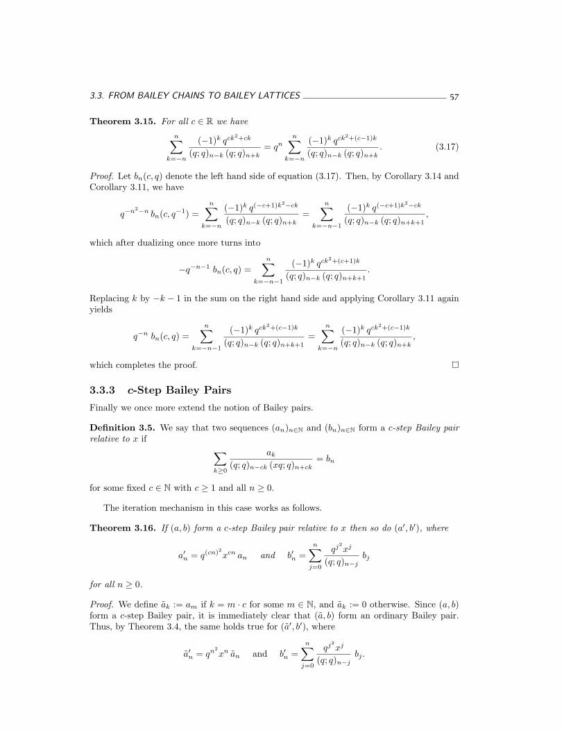
3.3. FROM BAILEY CHAINS TO BAILEY LATTICES 57
Theorem 3.15. For all c ∈ R we haven∑
k=−n
(−1)k qck2+ck
(q; q)n−k (q; q)n+k= qn
n∑
k=−n
(−1)k qck2+(c−1)k
(q; q)n−k (q; q)n+k. (3.17)
Proof. Let bn(c, q) denote the left hand side of equation (3.17). Then, by Corollary 3.14 andCorollary 3.11, we have
q−n2−n bn(c, q−1) =n∑
k=−n
(−1)k q(−c+1)k2−ck
(q; q)n−k (q; q)n+k=
n∑
k=−n−1
(−1)k q(−c+1)k2−ck
(q; q)n−k (q; q)n+k+1,
which after dualizing once more turns into
−q−n−1 bn(c, q) =n∑
k=−n−1
(−1)k qck2+(c+1)k
(q; q)n−k (q; q)n+k+1.
Replacing k by −k − 1 in the sum on the right hand side and applying Corollary 3.11 againyields
q−n bn(c, q) =n∑
k=−n−1
(−1)k qck2+(c−1)k
(q; q)n−k (q; q)n+k+1=
n∑
k=−n
(−1)k qck2+(c−1)k
(q; q)n−k (q; q)n+k,
which completes the proof.
3.3.3 c-Step Bailey Pairs
Finally we once more extend the notion of Bailey pairs.
Definition 3.5. We say that two sequences (an)n∈N and (bn)n∈N form a c-step Bailey pairrelative to x if
∑
k≥0
ak
(q; q)n−ck (xq; q)n+ck= bn
for some fixed c ∈ N with c ≥ 1 and all n ≥ 0.
The iteration mechanism in this case works as follows.
Theorem 3.16. If (a, b) form a c-step Bailey pair relative to x then so do (a′, b′), where
a′n = q(cn)2xcn an and b′n =n∑
j=0
qj2xj
(q; q)n−jbj
for all n ≥ 0.
Proof. We define ak := am if k = m · c for some m ∈ N, and ak := 0 otherwise. Since (a, b)form a c-step Bailey pair, it is immediately clear that (a, b) form an ordinary Bailey pair.Thus, by Theorem 3.4, the same holds true for (a′, b′), where
a′n = qn2xn an and b′n =
n∑
j=0
qj2xj
(q; q)n−jbj .
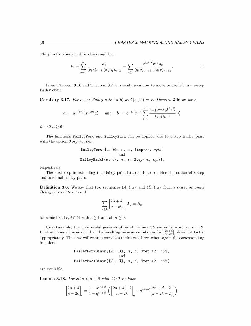
58 CHAPTER 3. WALKING ALONG BAILEY CHAINS
The proof is completed by observing that
b′n =n∑
k=0
a′k(q; q)n−k (xq; q)n+k
=∑
k≥0
q(ck)2xck ak
(q; q)n−ck (xq; q)n+ck.
From Theorem 3.16 and Theorem 3.7 it is easily seen how to move to the left in a c-stepBailey chain.
Corollary 3.17. For c-step Bailey pairs (a, b) and (a′, b′) as in Theorem 3.16 we have
an = q−(cn)2x−cn a′n and bn = q−n2x−n
n∑
j=0
(−1)n−j q(n−j
2 )
(q; q)n−jb′j
for all n ≥ 0.
The functions BaileyForw and BaileyBack can be applied also to c-step Bailey pairswith the option Step->c, i.e.,
BaileyForw[{a, b}, n, x, Step->c, opts]and
BaileyBack[{a, b}, n, x, Step->c, opts],
respectively.The next step in extending the Bailey pair database is to combine the notion of c-step
and binomial Bailey pairs.
Definition 3.6. We say that two sequences (An)n∈N and (Bn)n∈N form a c-step binomialBailey pair relative to d if
∑
k≥0
[2n + d
n− ck
]
q
Ak = Bn
for some fixed c, d ∈ N with c ≥ 1 and all n ≥ 0.
Unfortunately, the only useful generalization of Lemma 3.9 seems to exist for c = 2.In other cases it turns out that the resulting recurrence relation for
[2n+dn−ck
]q
does not factorappropriately. Thus, we will restrict ourselves to this case here, where again the correspondingfunctions
BaileyForwBinom[{A, B}, n, d, Step->2, opts]and
BaileyBackBinom[{A, B}, n, d, Step->2, opts]
are available.
Lemma 3.18. For all n, k, d ∈ N with d ≥ 2 we have[2n + d
n− 2k
]
q
=1− q2n+d
1− q4k+d
([2n + d− 2
n− 2k
]
q
− q4k+d
[2n + d− 2n− 2k − 2
]
q
).
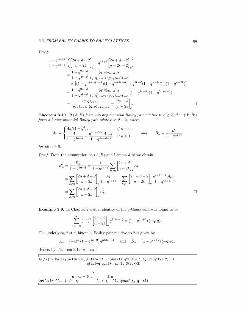
3.3. FROM BAILEY CHAINS TO BAILEY LATTICES 59
Proof.
1− q2n+d
1− q4k+d
([2n + d− 2
n− 2k
]
q
− q4k+d
[2n + d− 2n− 2k − 2
]
q
)
=1− q2n+d
1− q4k+d
(q; q)2n+d−2
(q; q)n−2k (q; q)n+2k+d
× [(1− qn+2k+d−1)(1− qn+2k+d)− q4k+d(1− qn−2k−1)(1− qn−2k)
]
=1− q2n+d
1− q4k+d
(q; q)2n+d−2
(q; q)n−2k (q; q)n+2k+d(1− q4k+d)(1− q2n+d−1)
=(q; q)2n+d
(q; q)n−2k (q; q)n+2k+d=
[2n + d
n− 2k
]
q
.
Theorem 3.19. If (A,B) form a 2-step binomial Bailey pair relative to d ≥ 2, then (A′, B′)form a 2-step binomial Bailey pair relative to d− 2, where
A′n =
A0/(1− qd), if n = 0,
An
1− q4n+d− q4n+d−4 An−1
1− q4n+d−4if n ≥ 1,
and B′n =
Bn
1− q2n+d
for all n ≥ 0.
Proof. From the assumption on (A,B) and Lemma 3.18 we obtain
B′n =
Bn
1− q2n+d=
11− q2n+d
∑
k≥0
[2n + d
n− 2k
]
q
Ak
=∑
k≥0
[2n + d− 2
n− 2k
]
q
Ak
1− q4k+d−
∑
k≥1
[2n + d− 2
n− 2k
]
q
q4k+d−4 Ak−1
1− q4k+d−4
=∑
k≥0
[2n + d− 2
n− 2k
]
q
A′k.
Example 3.9. In Chapter 2 a dual identity of the q-Gauss sum was found to be
∞∑
k=−∞(−1)k
[2n + 2n− 2k
]
q
qk(3k+1) = (1− q2n+2) (−q; q)n.
The underlying 2-step binomial Bailey pair relative to 2 is given by
An = (−1)n (1− q4n+2) qn(3n+1) and Bn = (1− q2n+2) (−q; q)n.
Hence, by Theorem 3.19, we have:
In[17]:= BaileyBackBinom[{(-1)^n (1-q^(4n+2)) q^(n(3n+1)), (1-q^(2n+2)) *
qfac[-q,q,n]}, n, 2, Step->2]
2
n -n + 3 n 2 n
Out[17]= {{1, (-1) q (1 + q )}, qfac[-q, q, n]}
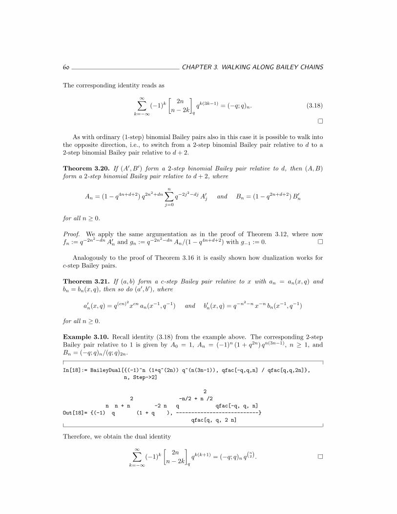
60 CHAPTER 3. WALKING ALONG BAILEY CHAINS
The corresponding identity reads as
∞∑
k=−∞(−1)k
[2n
n− 2k
]
q
qk(3k−1) = (−q; q)n. (3.18)
As with ordinary (1-step) binomial Bailey pairs also in this case it is possible to walk intothe opposite direction, i.e., to switch from a 2-step binomial Bailey pair relative to d to a2-step binomial Bailey pair relative to d + 2.
Theorem 3.20. If (A′, B′) form a 2-step binomial Bailey pair relative to d, then (A,B)form a 2-step binomial Bailey pair relative to d + 2, where
An = (1− q4n+d+2) q2n2+dnn∑
j=0
q−2j2−dj A′j and Bn = (1− q2n+d+2)B′n
for all n ≥ 0.
Proof. We apply the same argumentation as in the proof of Theorem 3.12, where nowfn := q−2n2−dn A′n and gn := q−2n2−dn An/(1− q4n+d+2) with g−1 := 0.
Analogously to the proof of Theorem 3.16 it is easily shown how dualization works forc-step Bailey pairs.
Theorem 3.21. If (a, b) form a c-step Bailey pair relative to x with an = an(x, q) andbn = bn(x, q), then so do (a′, b′), where
a′n(x, q) = q(cn)2xcn an(x−1, q−1) and b′n(x, q) = q−n2−n x−n bn(x−1, q−1)
for all n ≥ 0.
Example 3.10. Recall identity (3.18) from the example above. The corresponding 2-stepBailey pair relative to 1 is given by A0 = 1, An = (−1)n (1 + q2n) qn(3n−1), n ≥ 1, andBn = (−q; q)n/(q; q)2n.
In[18]:= BaileyDual[{(-1)^n (1+q^(2n)) q^(n(3n-1)), qfac[-q,q,n] / qfac[q,q,2n]},
n, Step->2]
2
2 -n/2 + n /2
n n + n -2 n q qfac[-q, q, n]
Out[18]= {(-1) q (1 + q ), ---------------------------}
qfac[q, q, 2 n]
Therefore, we obtain the dual identity
∞∑
k=−∞(−1)k
[2n
n− 2k
]
q
qk(k+1) = (−q; q)n q(n2).
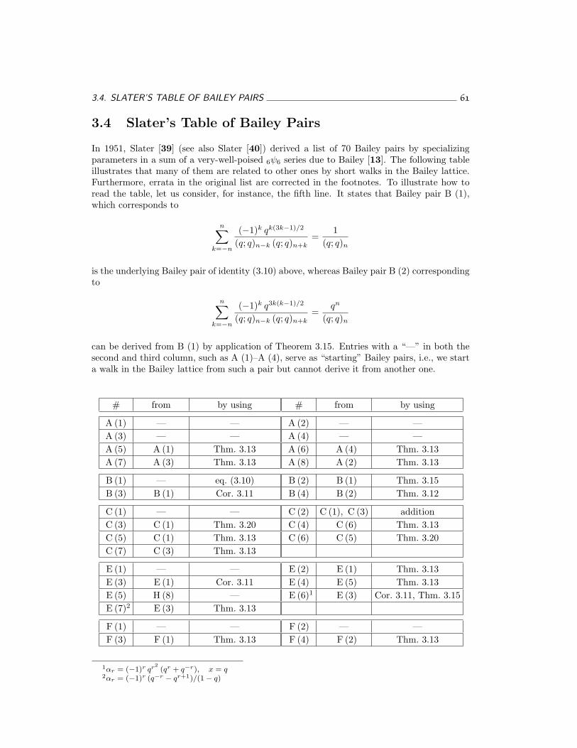
3.4. SLATER’S TABLE OF BAILEY PAIRS 61
3.4 Slater’s Table of Bailey Pairs
In 1951, Slater [39] (see also Slater [40]) derived a list of 70 Bailey pairs by specializingparameters in a sum of a very-well-poised 6ψ6 series due to Bailey [13]. The following tableillustrates that many of them are related to other ones by short walks in the Bailey lattice.Furthermore, errata in the original list are corrected in the footnotes. To illustrate how toread the table, let us consider, for instance, the fifth line. It states that Bailey pair B (1),which corresponds to
n∑
k=−n
(−1)k qk(3k−1)/2
(q; q)n−k (q; q)n+k=
1(q; q)n
is the underlying Bailey pair of identity (3.10) above, whereas Bailey pair B (2) correspondingto
n∑
k=−n
(−1)k q3k(k−1)/2
(q; q)n−k (q; q)n+k=
qn
(q; q)n
can be derived from B (1) by application of Theorem 3.15. Entries with a “—” in both thesecond and third column, such as A (1)–A (4), serve as “starting” Bailey pairs, i.e., we starta walk in the Bailey lattice from such a pair but cannot derive it from another one.
# from by using
A (1) — —A (3) — —A (5) A (1) Thm. 3.13A (7) A (3) Thm. 3.13
B (1) — eq. (3.10)B (3) B (1) Cor. 3.11
C (1) — —C (3) C (1) Thm. 3.20C (5) C (1) Thm. 3.13C (7) C (3) Thm. 3.13
E (1) — —E (3) E (1) Cor. 3.11E (5) H (8) —E (7)2 E (3) Thm. 3.13
F (1) — —F (3) F (1) Thm. 3.13
# from by using
A (2) — —A (4) — —A (6) A (4) Thm. 3.13A (8) A (2) Thm. 3.13
B (2) B (1) Thm. 3.15B (4) B (2) Thm. 3.12
C (2) C (1), C (3) additionC (4) C (6) Thm. 3.13C (6) C (5) Thm. 3.20
E (2) E (1) Thm. 3.13E (4) E (5) Thm. 3.13E (6)1 E (3) Cor. 3.11, Thm. 3.15
F (2) — —F (4) F (2) Thm. 3.13
1αr = (−1)r qr2(qr + q−r), x = q
2αr = (−1)r (q−r − qr+1)/(1− q)
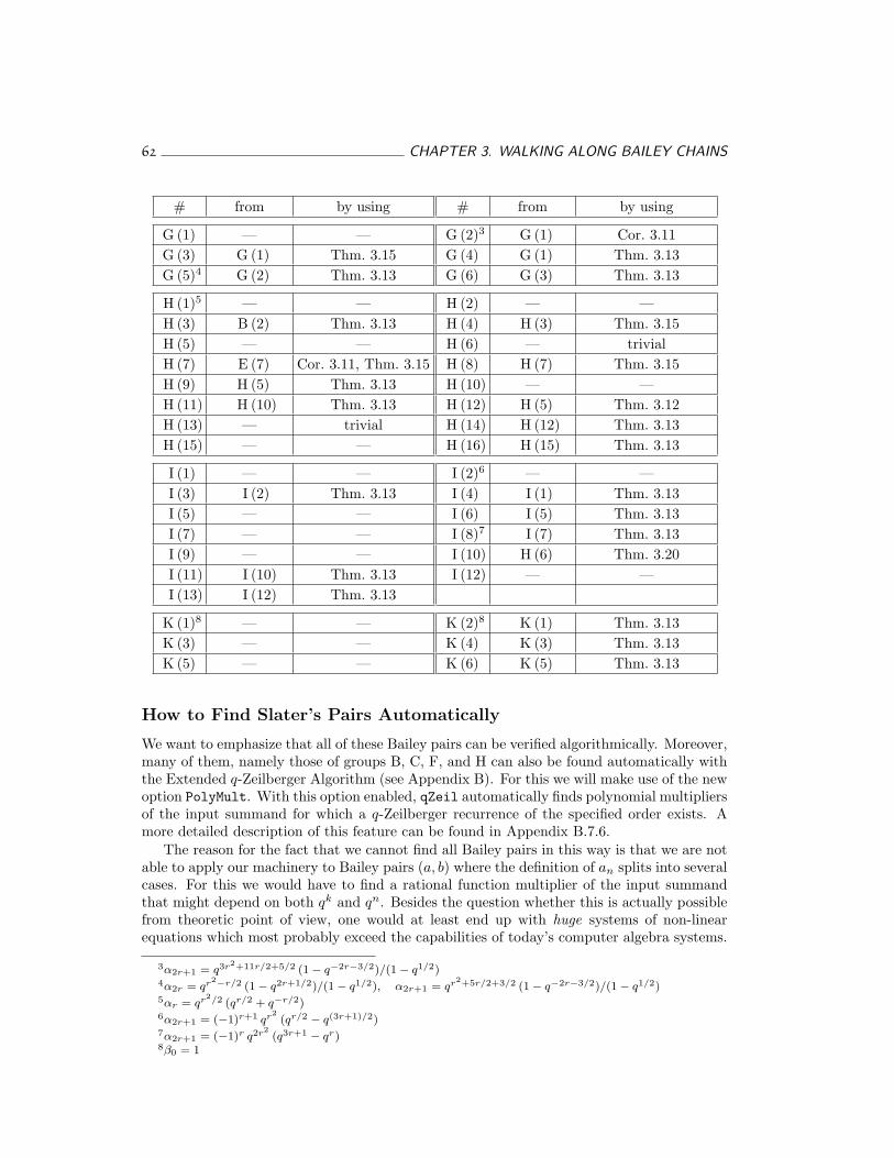
62 CHAPTER 3. WALKING ALONG BAILEY CHAINS
# from by using
G (1) — —G (3) G (1) Thm. 3.15G (5)4 G (2) Thm. 3.13
H (1)5 — —H (3) B (2) Thm. 3.13H (5) — —H (7) E (7) Cor. 3.11, Thm. 3.15H (9) H (5) Thm. 3.13H (11) H (10) Thm. 3.13H (13) — trivialH (15) — —
I (1) — —I (3) I (2) Thm. 3.13I (5) — —I (7) — —I (9) — —I (11) I (10) Thm. 3.13I (13) I (12) Thm. 3.13
K (1)8 — —K (3) — —K (5) — —
# from by using
G (2)3 G (1) Cor. 3.11G (4) G (1) Thm. 3.13G (6) G (3) Thm. 3.13
H (2) — —H (4) H (3) Thm. 3.15H (6) — trivialH (8) H (7) Thm. 3.15H (10) — —H (12) H (5) Thm. 3.12H (14) H (12) Thm. 3.13H (16) H (15) Thm. 3.13
I (2)6 — —I (4) I (1) Thm. 3.13I (6) I (5) Thm. 3.13I (8)7 I (7) Thm. 3.13I (10) H (6) Thm. 3.20I (12) — —
K (2)8 K (1) Thm. 3.13K (4) K (3) Thm. 3.13K (6) K (5) Thm. 3.13
How to Find Slater’s Pairs Automatically
We want to emphasize that all of these Bailey pairs can be verified algorithmically. Moreover,many of them, namely those of groups B, C, F, and H can also be found automatically withthe Extended q-Zeilberger Algorithm (see Appendix B). For this we will make use of the newoption PolyMult. With this option enabled, qZeil automatically finds polynomial multipliersof the input summand for which a q-Zeilberger recurrence of the specified order exists. Amore detailed description of this feature can be found in Appendix B.7.6.
The reason for the fact that we cannot find all Bailey pairs in this way is that we are notable to apply our machinery to Bailey pairs (a, b) where the definition of an splits into severalcases. For this we would have to find a rational function multiplier of the input summandthat might depend on both qk and qn. Besides the question whether this is actually possiblefrom theoretic point of view, one would at least end up with huge systems of non-linearequations which most probably exceed the capabilities of today’s computer algebra systems.
3α2r+1 = q3r2+11r/2+5/2 (1− q−2r−3/2)/(1− q1/2)4α2r = qr2−r/2 (1− q2r+1/2)/(1− q1/2), α2r+1 = qr2+5r/2+3/2 (1− q−2r−3/2)/(1− q1/2)5αr = qr2/2 (qr/2 + q−r/2)6α2r+1 = (−1)r+1 qr2
(qr/2 − q(3r+1)/2)7α2r+1 = (−1)r q2r2
(q3r+1 − qr)8β0 = 1
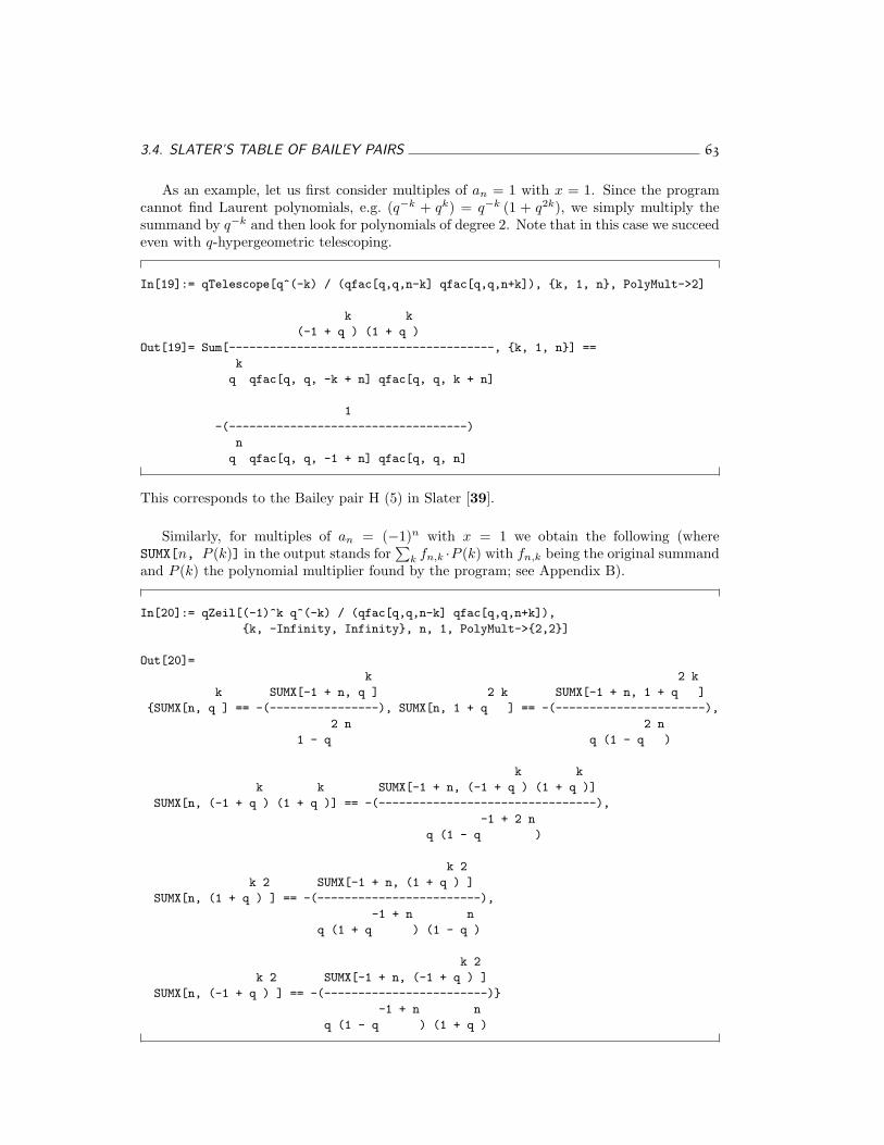
3.4. SLATER’S TABLE OF BAILEY PAIRS 63
As an example, let us first consider multiples of an = 1 with x = 1. Since the programcannot find Laurent polynomials, e.g. (q−k + qk) = q−k (1 + q2k), we simply multiply thesummand by q−k and then look for polynomials of degree 2. Note that in this case we succeedeven with q-hypergeometric telescoping.
In[19]:= qTelescope[q^(-k) / (qfac[q,q,n-k] qfac[q,q,n+k]), {k, 1, n}, PolyMult->2]
k k
(-1 + q ) (1 + q )
Out[19]= Sum[---------------------------------------, {k, 1, n}] ==
k
q qfac[q, q, -k + n] qfac[q, q, k + n]
1
-(-----------------------------------)
n
q qfac[q, q, -1 + n] qfac[q, q, n]
This corresponds to the Bailey pair H (5) in Slater [39].
Similarly, for multiples of an = (−1)n with x = 1 we obtain the following (whereSUMX[n, P (k)] in the output stands for
∑k fn,k ·P (k) with fn,k being the original summand
and P (k) the polynomial multiplier found by the program; see Appendix B).
In[20]:= qZeil[(-1)^k q^(-k) / (qfac[q,q,n-k] qfac[q,q,n+k]),
{k, -Infinity, Infinity}, n, 1, PolyMult->{2,2}]
Out[20]=
k 2 k
k SUMX[-1 + n, q ] 2 k SUMX[-1 + n, 1 + q ]
{SUMX[n, q ] == -(----------------), SUMX[n, 1 + q ] == -(----------------------),
2 n 2 n
1 - q q (1 - q )
k k
k k SUMX[-1 + n, (-1 + q ) (1 + q )]
SUMX[n, (-1 + q ) (1 + q )] == -(--------------------------------),
-1 + 2 n
q (1 - q )
k 2
k 2 SUMX[-1 + n, (1 + q ) ]
SUMX[n, (1 + q ) ] == -(------------------------),
-1 + n n
q (1 + q ) (1 - q )
k 2
k 2 SUMX[-1 + n, (-1 + q ) ]
SUMX[n, (-1 + q ) ] == -(------------------------)}
-1 + n n
q (1 - q ) (1 + q )
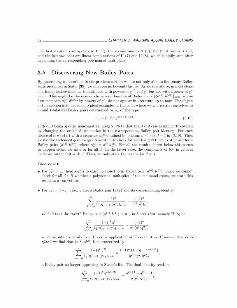
64 CHAPTER 3. WALKING ALONG BAILEY CHAINS
The first solution corresponds to H (7), the second one to H (8), the third one is trivial,and the last two ones are linear combinations of H (7) and H (8), which is easily seen afterexpanding the corresponding polynomial multipliers.
3.5 Discovering New Bailey Pairs
By proceeding as described in the previous section we are not only able to find many Baileypairs presented in Slater [39], we can even go beyond this list. As we saw above, in most stepsof a Bailey lattice walk, an is multiplied with powers of qn2
and qn but not with a power of qn
alone. This might be the reason why several families of Bailey pairs {(a(d), b(d))}d∈N, whosefirst members a(d)
n differ by powers of qn, do not appear in literature up to now. The objectof this section is to list some typical examples of this kind where we will restrict ourselves to0- and 1-bilateral Bailey pairs determined by an of the type
an = (±1)n qn(αn+β)/2, (3.19)
with α, β being specific non-negative integers. Note that the β < 0 case is implicitly coveredby changing the order of summation in the corresponding Bailey pair identity. For eachchoice of α we start with a sequence a(0)
n obtained by putting β = 0 or β = 1 in (3.19). Thenwe use the Extended q-Zeilberger Algorithm to check for which d ∈ N there exist closed formBailey pairs (a(d), b(d)), where a(d)
n = qdn a(0)n . For all the results shown below this seems
to happen either for no d or for all d. In the latter case, the complexity of b(d)n in general
increases rather fast with d. Thus, we only state the results for d ≤ 3.
Case α = 0:
• For a(0)n = 1, there seems to exist no closed form Bailey pair (a(d), b(d)). Since we cannot
check for all d ∈ N whether a polynomial multiplier of the summand exists, we state thisresult as a conjecture.
• For a(0)n = (−1)n, i.e., Slater’s Bailey pair H (7) and its corresponding identity
n∑
k=−n
(−1)k
(q; q)n−k (q; q)n+k=
(−1)n
(q2; q2)n,
we find that the “next” Bailey pair (a(1), b(1)) is still in Slater’s list, namely H (8) or
n∑
k=−n
(−1)k qk
(q; q)n−k (q; q)n+k=
(−1)n
qn (q2; q2)n,
which is obtained easily from H (7) by application of Theorem 3.15. However, thanks toqZeil we find that (a(2), b(2)) is characterized by
n∑
k=−n
(−1)k q2k
(q; q)n−k (q; q)n+k=
(−1)n(1 + q − q2n+1)
)
q2n (q2; q2)n,
a Bailey pair no longer appearing in Slater’s list. The dual identity reads as
n∑
k=−n
(−1)k qk(k+2)
(q; q)n−k (q; q)n+k=
q2n+1 + q2n − 1q (q2; q2)n
,
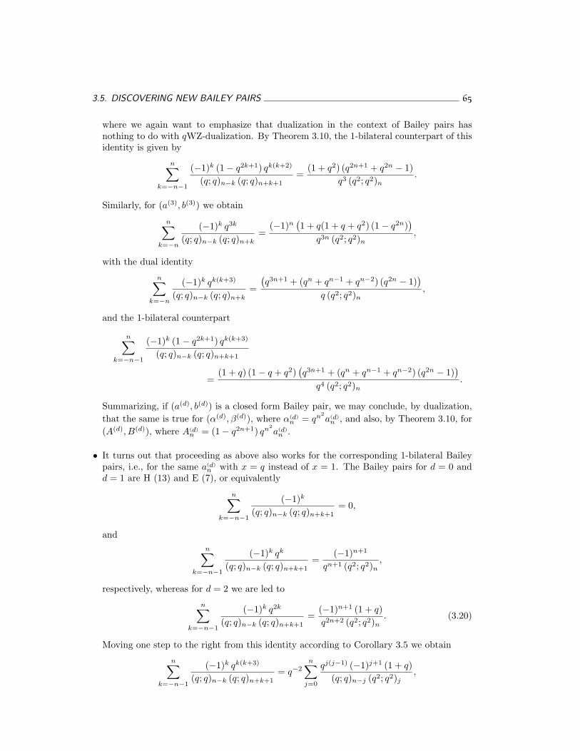
3.5. DISCOVERING NEW BAILEY PAIRS 65
where we again want to emphasize that dualization in the context of Bailey pairs hasnothing to do with qWZ-dualization. By Theorem 3.10, the 1-bilateral counterpart of thisidentity is given by
n∑
k=−n−1
(−1)k (1− q2k+1) qk(k+2)
(q; q)n−k (q; q)n+k+1=
(1 + q2) (q2n+1 + q2n − 1)q3 (q2; q2)n
.
Similarly, for (a(3), b(3)) we obtain
n∑
k=−n
(−1)k q3k
(q; q)n−k (q; q)n+k=
(−1)n(1 + q(1 + q + q2) (1− q2n)
)
q3n (q2; q2)n,
with the dual identity
n∑
k=−n
(−1)k qk(k+3)
(q; q)n−k (q; q)n+k=
(q3n+1 + (qn + qn−1 + qn−2) (q2n − 1)
)
q (q2; q2)n,
and the 1-bilateral counterpart
n∑
k=−n−1
(−1)k (1− q2k+1) qk(k+3)
(q; q)n−k (q; q)n+k+1
=(1 + q) (1− q + q2)
(q3n+1 + (qn + qn−1 + qn−2) (q2n − 1)
)
q4 (q2; q2)n.
Summarizing, if (a(d), b(d)) is a closed form Bailey pair, we may conclude, by dualization,that the same is true for (α(d), β(d)), where α(d)
n = qn2a(d)
n , and also, by Theorem 3.10, for(A(d), B(d)), where A(d)
n = (1− q2n+1) qn2a(d)
n .
• It turns out that proceeding as above also works for the corresponding 1-bilateral Baileypairs, i.e., for the same a(d)
n with x = q instead of x = 1. The Bailey pairs for d = 0 andd = 1 are H (13) and E (7), or equivalently
n∑
k=−n−1
(−1)k
(q; q)n−k (q; q)n+k+1= 0,
andn∑
k=−n−1
(−1)k qk
(q; q)n−k (q; q)n+k+1=
(−1)n+1
qn+1 (q2; q2)n,
respectively, whereas for d = 2 we are led to
n∑
k=−n−1
(−1)k q2k
(q; q)n−k (q; q)n+k+1=
(−1)n+1 (1 + q)q2n+2 (q2; q2)n
. (3.20)
Moving one step to the right from this identity according to Corollary 3.5 we obtain
n∑
k=−n−1
(−1)k qk(k+3)
(q; q)n−k (q; q)n+k+1= q−2
n∑
j=0
qj(j−1) (−1)j+1 (1 + q)(q; q)n−j (q2; q2)j
,
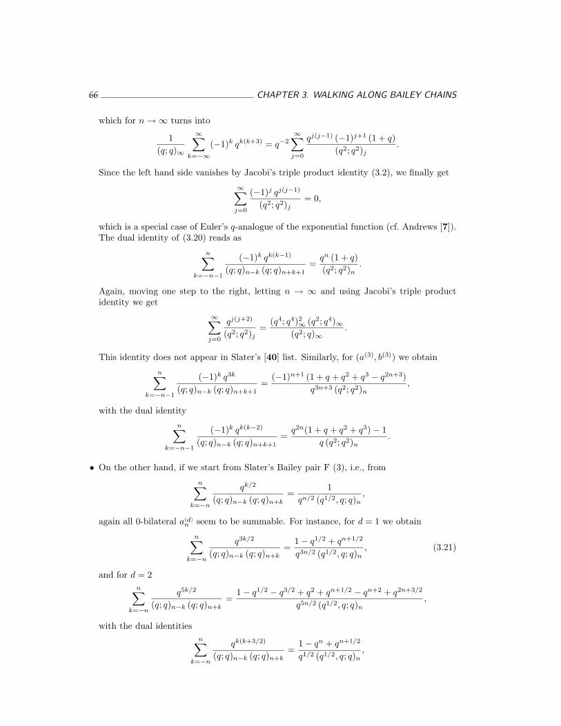
66 CHAPTER 3. WALKING ALONG BAILEY CHAINS
which for n →∞ turns into
1(q; q)∞
∞∑
k=−∞(−1)k qk(k+3) = q−2
∞∑
j=0
qj(j−1) (−1)j+1 (1 + q)(q2; q2)j
.
Since the left hand side vanishes by Jacobi’s triple product identity (3.2), we finally get
∞∑
j=0
(−1)j qj(j−1)
(q2; q2)j= 0,
which is a special case of Euler’s q-analogue of the exponential function (cf. Andrews [7]).The dual identity of (3.20) reads as
n∑
k=−n−1
(−1)k qk(k−1)
(q; q)n−k (q; q)n+k+1=
qn (1 + q)(q2; q2)n
.
Again, moving one step to the right, letting n → ∞ and using Jacobi’s triple productidentity we get
∞∑
j=0
qj(j+2)
(q2; q2)j=
(q4; q4)2∞ (q2; q4)∞(q2; q)∞
.
This identity does not appear in Slater’s [40] list. Similarly, for (a(3), b(3)) we obtain
n∑
k=−n−1
(−1)k q3k
(q; q)n−k (q; q)n+k+1=
(−1)n+1 (1 + q + q2 + q3 − q2n+3)q3n+3 (q2; q2)n
,
with the dual identity
n∑
k=−n−1
(−1)k qk(k−2)
(q; q)n−k (q; q)n+k+1=
q2n(1 + q + q2 + q3)− 1q (q2; q2)n
.
• On the other hand, if we start from Slater’s Bailey pair F (3), i.e., from
n∑
k=−n
qk/2
(q; q)n−k (q; q)n+k=
1qn/2 (q1/2, q; q)n
,
again all 0-bilateral a(d)n seem to be summable. For instance, for d = 1 we obtain
n∑
k=−n
q3k/2
(q; q)n−k (q; q)n+k=
1− q1/2 + qn+1/2
q3n/2 (q1/2, q; q)n, (3.21)
and for d = 2n∑
k=−n
q5k/2
(q; q)n−k (q; q)n+k=
1− q1/2 − q3/2 + q2 + qn+1/2 − qn+2 + q2n+3/2
q5n/2 (q1/2, q; q)n,
with the dual identitiesn∑
k=−n
qk(k+3/2)
(q; q)n−k (q; q)n+k=
1− qn + qn+1/2
q1/2 (q1/2, q; q)n,
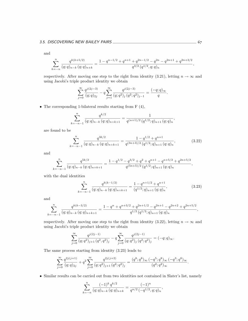
3.5. DISCOVERING NEW BAILEY PAIRS 67
andn∑
k=−n
qk(k+5/2)
(q; q)n−k (q; q)n+k=
1− qn−1/2 + qn+1 + q2n−1/2 − q2n − q2n+1 + q2n+3/2
q3/2 (q1/2, q; q)n,
respectively. After moving one step to the right from identity (3.21), letting n → ∞ andusing Jacobi’s triple product identity we obtain
∞∑
j=0
qj(2j−3)
(q; q)2j− q
∞∑
j=1
qj(2j−3)
(q; q2)j (q2; q2)j−1=
(−q; q)∞q
.
• The corresponding 1-bilateral results starting from F (4),
n∑
k=−n−1
qk/2
(q; q)n−k (q; q)n+k+1=
1q(n+1)/2 (q1/2; q)n+1 (q; q)n
,
are found to ben∑
k=−n−1
q3k/2
(q; q)n−k (q; q)n+k+1=
1− q1/2 + qn+1
q(3n+3)/2 (q1/2; q)n+1 (q; q)n, (3.22)
andn∑
k=−n−1
q5k/2
(q; q)n−k (q; q)n+k+1=
1− q1/2 − q3/2 + q2 + qn+1 − qn+5/2 + q2n+5/2
q(5n+5)/2 (q1/2; q)n+1 (q; q)n,
with the dual identitiesn∑
k=−n−1
qk(k−1/2)
(q; q)n−k (q; q)n+k+1=
1− qn+1/2 + qn+1
(q1/2; q)n+1 (q; q)n, (3.23)
andn∑
k=−n−1
qk(k−3/2)
(q; q)n−k (q; q)n+k+1=
1− qn + qn+3/2 + q2n+1/2 − q2n+1 − q2n+2 + q2n+5/2
q1/2 (q1/2; q)n+1 (q; q)n,
respectively. After moving one step to the right from identity (3.22), letting n → ∞ andusing Jacobi’s triple product identity we obtain
∞∑
j=0
qj(2j−1)
(q; q2)j+1 (q2, q2)j− q
∞∑
j=0
qj(2j−1)
(q; q2)j (q2; q2)j= (−q; q)∞.
The same process starting from identity (3.23) leads to
∞∑
j=0
q2j(j+1)
(q; q)2j+ q2
∞∑
j=0
q2j(j+2)
(q; q2)j+1 (q2; q2)j=
(q8; q8)∞ (−q5; q8)∞ (−q3; q8)∞(q2; q2)∞
.
• Similar results can be carried out from two identities not contained in Slater’s list, namely
n∑
k=−n
(−1)k qk/2
(q; q)n−k (q; q)n+k=
(−1)n
qn/2 (−q1/2, q; q)n,
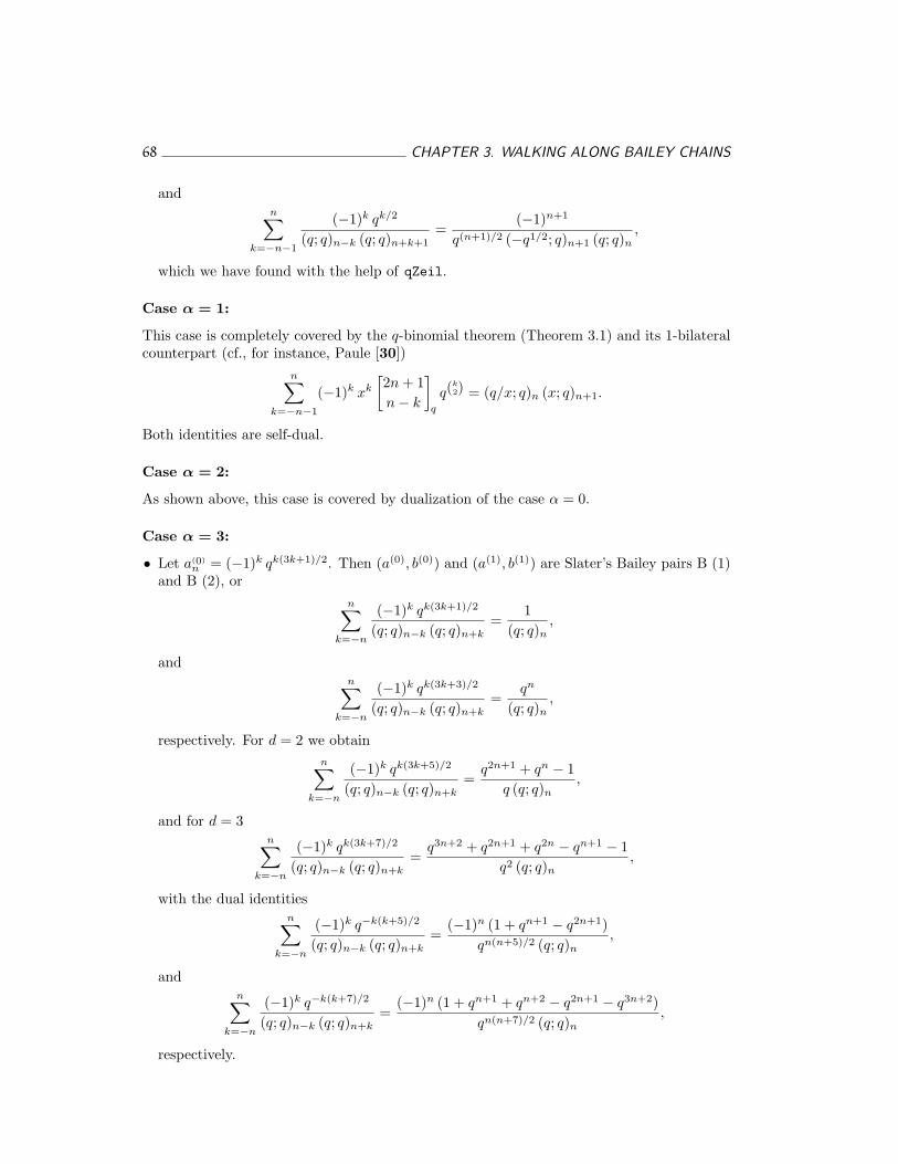
68 CHAPTER 3. WALKING ALONG BAILEY CHAINS
andn∑
k=−n−1
(−1)k qk/2
(q; q)n−k (q; q)n+k+1=
(−1)n+1
q(n+1)/2 (−q1/2; q)n+1 (q; q)n,
which we have found with the help of qZeil.
Case α = 1:
This case is completely covered by the q-binomial theorem (Theorem 3.1) and its 1-bilateralcounterpart (cf., for instance, Paule [30])
n∑
k=−n−1
(−1)k xk
[2n + 1n− k
]
q
q(k2) = (q/x; q)n (x; q)n+1.
Both identities are self-dual.
Case α = 2:
As shown above, this case is covered by dualization of the case α = 0.
Case α = 3:
• Let a(0)n = (−1)k qk(3k+1)/2. Then (a(0), b(0)) and (a(1), b(1)) are Slater’s Bailey pairs B (1)
and B (2), orn∑
k=−n
(−1)k qk(3k+1)/2
(q; q)n−k (q; q)n+k=
1(q; q)n
,
andn∑
k=−n
(−1)k qk(3k+3)/2
(q; q)n−k (q; q)n+k=
qn
(q; q)n,
respectively. For d = 2 we obtainn∑
k=−n
(−1)k qk(3k+5)/2
(q; q)n−k (q; q)n+k=
q2n+1 + qn − 1q (q; q)n
,
and for d = 3n∑
k=−n
(−1)k qk(3k+7)/2
(q; q)n−k (q; q)n+k=
q3n+2 + q2n+1 + q2n − qn+1 − 1q2 (q; q)n
,
with the dual identitiesn∑
k=−n
(−1)k q−k(k+5)/2
(q; q)n−k (q; q)n+k=
(−1)n (1 + qn+1 − q2n+1)qn(n+5)/2 (q; q)n
,
andn∑
k=−n
(−1)k q−k(k+7)/2
(q; q)n−k (q; q)n+k=
(−1)n (1 + qn+1 + qn+2 − q2n+1 − q3n+2)qn(n+7)/2 (q; q)n
,
respectively.
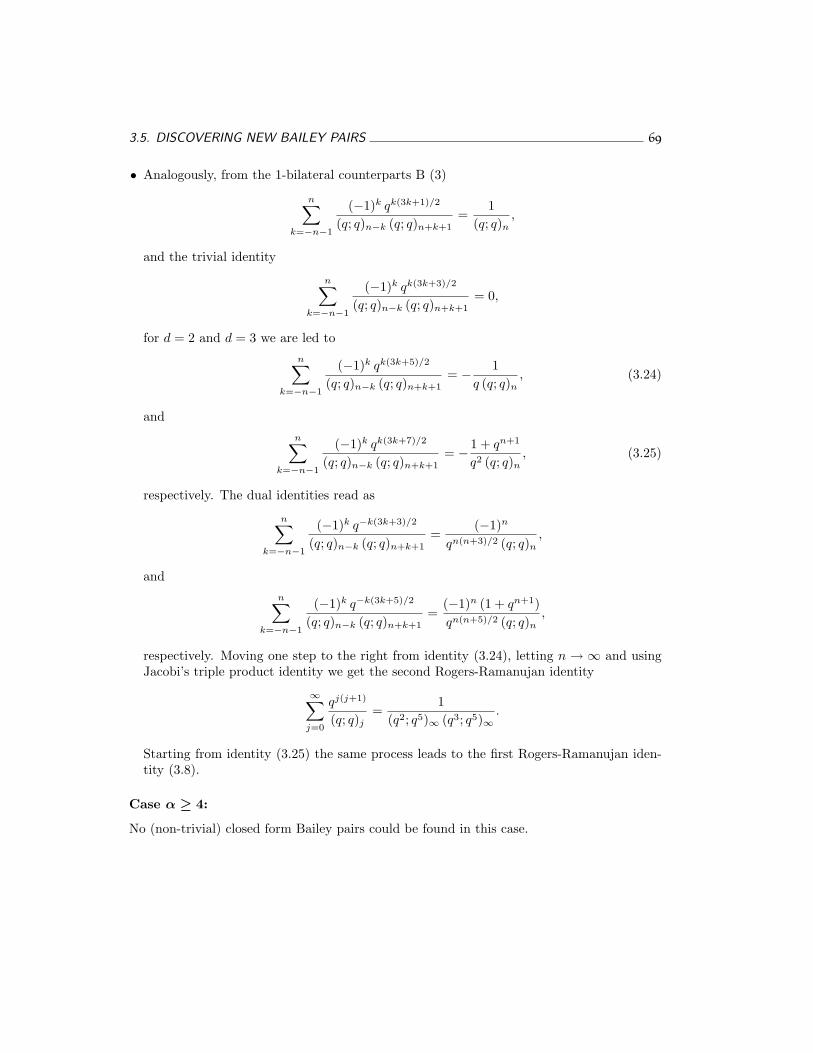
3.5. DISCOVERING NEW BAILEY PAIRS 69
• Analogously, from the 1-bilateral counterparts B (3)
n∑
k=−n−1
(−1)k qk(3k+1)/2
(q; q)n−k (q; q)n+k+1=
1(q; q)n
,
and the trivial identity
n∑
k=−n−1
(−1)k qk(3k+3)/2
(q; q)n−k (q; q)n+k+1= 0,
for d = 2 and d = 3 we are led ton∑
k=−n−1
(−1)k qk(3k+5)/2
(q; q)n−k (q; q)n+k+1= − 1
q (q; q)n, (3.24)
andn∑
k=−n−1
(−1)k qk(3k+7)/2
(q; q)n−k (q; q)n+k+1= − 1 + qn+1
q2 (q; q)n, (3.25)
respectively. The dual identities read as
n∑
k=−n−1
(−1)k q−k(3k+3)/2
(q; q)n−k (q; q)n+k+1=
(−1)n
qn(n+3)/2 (q; q)n,
andn∑
k=−n−1
(−1)k q−k(3k+5)/2
(q; q)n−k (q; q)n+k+1=
(−1)n (1 + qn+1)qn(n+5)/2 (q; q)n
,
respectively. Moving one step to the right from identity (3.24), letting n → ∞ and usingJacobi’s triple product identity we get the second Rogers-Ramanujan identity
∞∑
j=0
qj(j+1)
(q; q)j=
1(q2; q5)∞ (q3; q5)∞
.
Starting from identity (3.25) the same process leads to the first Rogers-Ramanujan iden-tity (3.8).
Case α ≥ 4:
No (non-trivial) closed form Bailey pairs could be found in this case.

70
71
Appendix A
A Note on q-BinomialCoefficients
Since q-binomial coefficients[nk
]q
play a fundamental role in q-hypergeometric summation,we shall briefly outline in this chapter how to generalize them to arbitrary integers n andk as well as to complex parameters. The former is needed, for instance, in the q-Zeilbergeralgorithm for evaluating q-hypergeometric sequences involving q-binomial coefficients at theboundary points of the summation interval.
Definition A.1. For n, k ∈ Z, let the q-binomial coefficient of n and k be given by
[n
k
]
q
:= limδ→1
(δq; q)n
(q; q)k (δq; q)n−k. (A.1)
Clearly, if n ≥ 0, equation (A.1) reduces to the usual definition of q-binomial coefficients,
[n
k
]
q
=(q; q)n
(q; q)k (q; q)n−k.
Note that the symmetry property for q-binomial coefficients,
[n
k
]
q
=[
n
n− k
]
q
only holds for non-negative n. For instance, we have[n0
]q
= 1, but[nn
]q
= 0 for all nega-tive n. However, the well-known recurrences for q-binomial coefficients are still satisfied forall integers n and k as stated in the following theorem.
Theorem A.1. For n, k ∈ Z, we have
[n + 1
k
]
q
=[n
k
]
q
qk +[
n
k − 1
]
q
=[n
k
]
q
+[
n
k − 1
]
q
qn+1−k.

72 APPENDIX A. A NOTE ON q-BINOMIAL COEFFICIENTS
Proof.[n
k
]
q
qk = limδ→1
(δq; q)n
(q; q)k (δq; q)n−k
1− δqn+1−k
1− δqn+1−kqk
= limδ→1
(δq; q)n
(q; q)k (δq; q)n+1−k
((1− δqn+1)− (1− qk)
)
=[n + 1
k
]
q
−[
n
k − 1
]
q
;
[n
k − 1
]
q
qn+1−k = limδ→1
(δq; q)n
(q; q)k−1 (δq; q)n+1−k
1− qk
1− qkδqn+1−k
= limδ→1
(δq; q)n
(q; q)k (δq; q)n+1−k
((1− δqn+1)− (1− δqn+1−k)
)
=[n + 1
k
]
q
−[n
k
]
q
.
Furthermore, the q-binomial coefficients might also be generalized to complex parame-ters. This has been already done by Gasper and Rahman [20], however, with the definitionpresented there,
[α
β
]
q
=(qβ+1, qα−β+1; q)∞
(q, qα+1; q)∞,
we get into trouble if α is a negative integer, because the denominator becomes 0 then.To overcome this problem we first introduce a q-analogue of the gamma function (see,
e.g., Askey [12] or Gasper and Rahman [20]).
Definition A.2. For x ∈ C, the q-gamma function is given by
Γq(x) :=(q; q)∞(qx; q)∞
(1− q)1−x,
when 0 < q < 1.
From this definition it follows directly that Γq satisfies the functional equation
Γq(x + 1) =1− qx
1− qΓq(x), Γq(1) = 1, (A.2)
the q-counterpart of the well-known functional equation for the gamma function
Γ(x + 1) = xΓ(x), Γ(1) = 1.
Furthermore, for n ∈ N we have
Γq(n + 1) = [n]q!,
where [n]q! denotes the q-factorial defined as [n]q! = 1·(1+q)·(1+q+q2) · · · (1+q+· · ·+qn−1)which trivially turns into Γ(n + 1) = n! for q = 1. Obviously, the q-gamma function haspoles at x = 0,−1,−2, etc. The q-binomial coefficient for complex parameters could then bedefined as follows.
73
Definition A.3. For α, β ∈ C, the q-binomial coefficient of α and β is given by[α
β
]
q
:= limε→0
Γq(α + 1 + ε)Γq(β + 1)Γq(α− β + 1 + ε)
,
where it is assumed that β is an integer whenever α is a negative integer.
This is a q-analogue of the extended definition for ordinary binomial coefficients,(
α
β
):= lim
ε→0
Γ(α + 1 + ε)Γ(β + 1)Γ(α− β + 1 + ε)
,
which has been used, for instance, by Wegschaider [42].
Theorem A.2. For α, β ∈ C, we have[α + 1
β
]
q
=[α
β
]
q
qβ +[
α
β − 1
]
q
=[α
β
]
q
+[
α
β − 1
]
q
qα+1−β .
Proof. This is easily seen by proceeding as in the proof of Theorem A.1 and using rela-tion (A.2).

74
75
Appendix B
How to Use qZeil
In the following we shall describe the usage of the author’s Mathematica implementation ofthe Extended q-Zeilberger Algorithm. Parts of this manual have been taken from an articleby Paule and Riese [33] and the author’s diploma thesis [37]. The latest version is availableby email request to the author†. Additional information can be retrieved via the World WideWeb from the qZeil homepage‡.
B.1 Package Structure and Installation
The package consists of five files named qZeil.m, qTelescope.m, qInput.m, qSimplify.m,and LinSolve.m, which have to be copied into one directory. After starting a Mathematicasession from this directory and typing <<qZeil.m all files (including the add-on packageBailey.m described in Chapter 3) are loaded automatically.
The whole package has been adapted for Mathematica 3.0. Since notebooks are nowmachine independent, the collection of examples (formerly known as qZeilExamples.txt) isdistributed in notebook format as qZeilExamples.nb. At the moment this notebook containsinput for about 500 identities. This also means that this set serves as a test suite for eachupdate of the package. Furthermore, the package is accompanied by the file WhatsNew.txtwhich describes all the changes since version 1.4.
The source files qTelescope.m and qSimplify.m may be renamed to qtelesco.m andqsimplif.m, respectively, if the system has troubles with file names not matching the “8.3”(MS-DOS) naming scheme.
B.2 Interfaces
The package has two interfaces. The user can invoke q-hypergeometric telescoping to finda closed form for a sum, or Zeilberger’s algorithm to come up with a recurrence for a sum.The corresponding commands are given by
qTelescope[summand, range, intconst, opts]and
qZeil[summand, range, n, order, intconst, opts],
†[email protected]‡http://www.risc.uni-linz.ac.at/research/combinat/risc/software/qZeil
76 APPENDIX B. HOW TO USE qZeil
where the parameters intconst and opts are optional arguments.
B.3 The Summand
Let K = Q(κ1, . . . , κm) denote the field of rational functions over the rational numbers Q in afixed number of indeterminates κ1, . . . , κm all different from q, k, and qk. The transcendentalextension of K by the indeterminate q is denoted by F , i.e., F = K(q).
In the present implementation we allow as summand for qTelescope any q-hypergeomet-ric sequence (fk)k∈Z of the form
fk =∏
r(Cr q(crir)k+dr ; qir )ark+br∏s(Ds q(vsjs)k+ws ; qjs)tsk+us
·R(qk) · qα(k2) · zk, (B.1)
withCr, Ds power products in K,ar, ts specific integers (i.e., integers free of any parameters),br, us integers, which may depend on parameters free of k,cr, dr, vs, ws specific integers,ir, js specific non-zero integers,R a rational function in F (qk) such that the denominator factors completely
into a product of terms of the form (1−D qvk+w),α specific integer, andz a rational function in F .
As summand for qZeil we allow any q-hypergeometric sequence (fn,k)n∈N,k∈Z (where weadditionally assume that the κi are different from n and qn) of the form
fn,k =∏
r(Cr q(drir)n+(erir)k+lr ; qir )arn+brk+cr∏s(Ds q(fsjs)n+(gsjs)k+ms ; qjs)usn+vsk+ws
·R(qn, qk) · qα(k2)+βnk · zk, (B.2)
withCr, Ds power products in K,ar, br, us, vs specific integers (i.e., integers free of any parameters),cr, ws integers, which may depend on parameters free of n and k,dr, er, fs, gs specific integers,lr,ms integers free of n and k,ir, js specific non-zero integers,R a rational function in F (qn, qk) such that the denominator factors
completely into a product of terms of the form (1−D qfn+gk+m),α, β specific integers, andz a rational function in F .
The q-shifted factorial (a; qi)m has to be typed as qfac[a,q^i,m]. In addition we al-low terms of the form qBrackets[a,q] for [a]q := (1 − qa)/(1 − q), qFactorial[a,q] for[a]q! := [1]q [2]q · · · [a]q, and qBinomial[a,b,q] for
[ab
]q, provided that those expressions can
be translated correctly — with respect to (B.1) or (B.2) — into terms of q-shifted factorials.Note that also for these forms powers q^i are admitted.
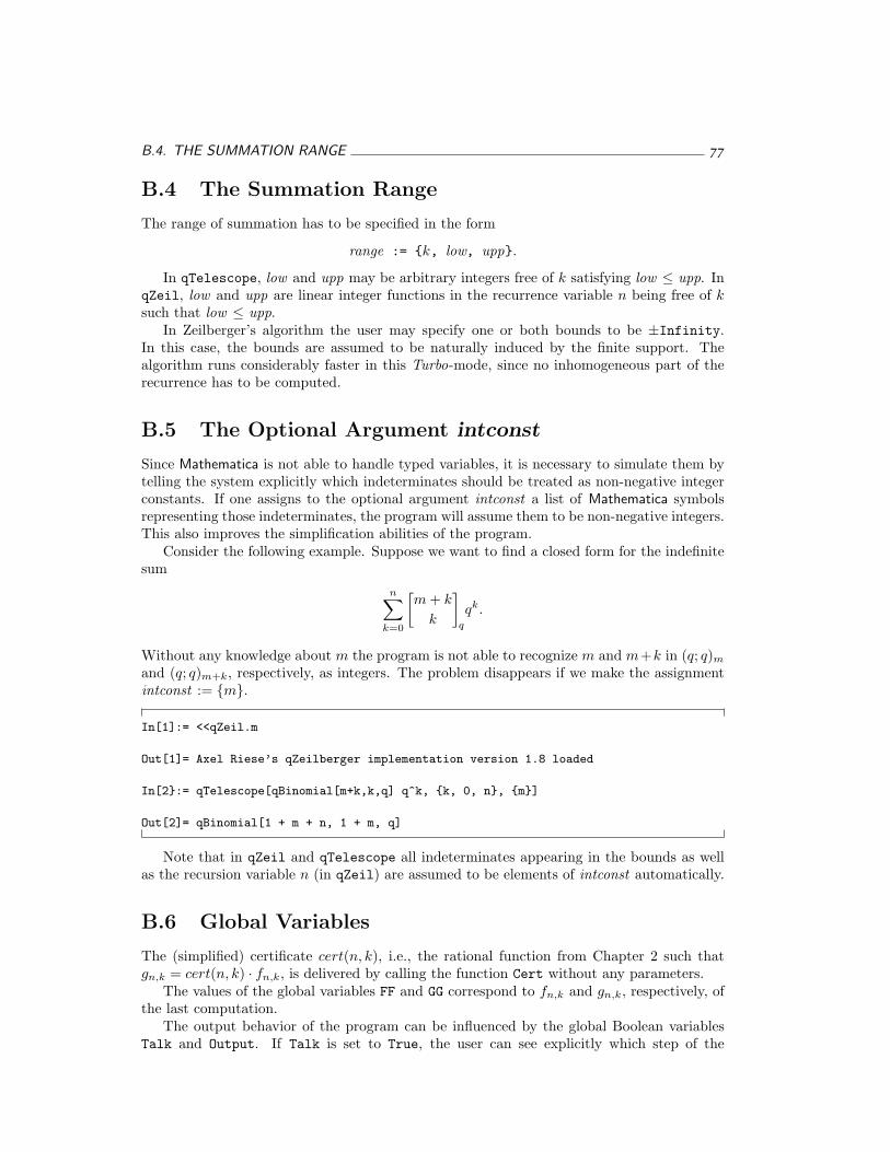
B.4. THE SUMMATION RANGE 77
B.4 The Summation Range
The range of summation has to be specified in the form
range := {k, low, upp}.
In qTelescope, low and upp may be arbitrary integers free of k satisfying low ≤ upp. InqZeil, low and upp are linear integer functions in the recurrence variable n being free of ksuch that low ≤ upp.
In Zeilberger’s algorithm the user may specify one or both bounds to be ±Infinity.In this case, the bounds are assumed to be naturally induced by the finite support. Thealgorithm runs considerably faster in this Turbo-mode, since no inhomogeneous part of therecurrence has to be computed.
B.5 The Optional Argument intconst
Since Mathematica is not able to handle typed variables, it is necessary to simulate them bytelling the system explicitly which indeterminates should be treated as non-negative integerconstants. If one assigns to the optional argument intconst a list of Mathematica symbolsrepresenting those indeterminates, the program will assume them to be non-negative integers.This also improves the simplification abilities of the program.
Consider the following example. Suppose we want to find a closed form for the indefinitesum
n∑
k=0
[m + k
k
]
q
qk.
Without any knowledge about m the program is not able to recognize m and m+k in (q; q)m
and (q; q)m+k, respectively, as integers. The problem disappears if we make the assignmentintconst := {m}.
In[1]:= <<qZeil.m
Out[1]= Axel Riese’s qZeilberger implementation version 1.8 loaded
In[2}:= qTelescope[qBinomial[m+k,k,q] q^k, {k, 0, n}, {m}]
Out[2]= qBinomial[1 + m + n, 1 + m, q]
Note that in qZeil and qTelescope all indeterminates appearing in the bounds as wellas the recursion variable n (in qZeil) are assumed to be elements of intconst automatically.
B.6 Global Variables
The (simplified) certificate cert(n, k), i.e., the rational function from Chapter 2 such thatgn,k = cert(n, k) · fn,k, is delivered by calling the function Cert without any parameters.
The values of the global variables FF and GG correspond to fn,k and gn,k, respectively, ofthe last computation.
The output behavior of the program can be influenced by the global Boolean variablesTalk and Output. If Talk is set to True, the user can see explicitly which step of the
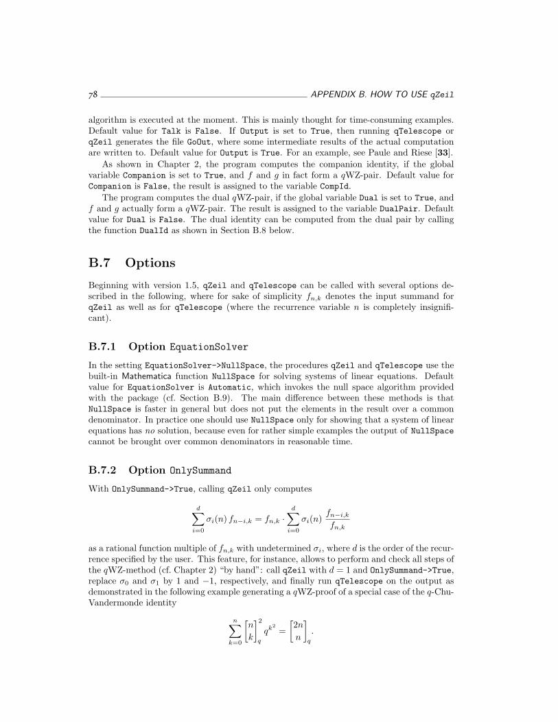
78 APPENDIX B. HOW TO USE qZeil
algorithm is executed at the moment. This is mainly thought for time-consuming examples.Default value for Talk is False. If Output is set to True, then running qTelescope orqZeil generates the file GoOut, where some intermediate results of the actual computationare written to. Default value for Output is True. For an example, see Paule and Riese [33].
As shown in Chapter 2, the program computes the companion identity, if the globalvariable Companion is set to True, and f and g in fact form a qWZ-pair. Default value forCompanion is False, the result is assigned to the variable CompId.
The program computes the dual qWZ-pair, if the global variable Dual is set to True, andf and g actually form a qWZ-pair. The result is assigned to the variable DualPair. Defaultvalue for Dual is False. The dual identity can be computed from the dual pair by callingthe function DualId as shown in Section B.8 below.
B.7 Options
Beginning with version 1.5, qZeil and qTelescope can be called with several options de-scribed in the following, where for sake of simplicity fn,k denotes the input summand forqZeil as well as for qTelescope (where the recurrence variable n is completely insignifi-cant).
B.7.1 Option EquationSolver
In the setting EquationSolver->NullSpace, the procedures qZeil and qTelescope use thebuilt-in Mathematica function NullSpace for solving systems of linear equations. Defaultvalue for EquationSolver is Automatic, which invokes the null space algorithm providedwith the package (cf. Section B.9). The main difference between these methods is thatNullSpace is faster in general but does not put the elements in the result over a commondenominator. In practice one should use NullSpace only for showing that a system of linearequations has no solution, because even for rather simple examples the output of NullSpacecannot be brought over common denominators in reasonable time.
B.7.2 Option OnlySummand
With OnlySummand->True, calling qZeil only computes
d∑
i=0
σi(n) fn−i,k = fn,k ·d∑
i=0
σi(n)fn−i,k
fn,k
as a rational function multiple of fn,k with undetermined σi, where d is the order of the recur-rence specified by the user. This feature, for instance, allows to perform and check all steps ofthe qWZ-method (cf. Chapter 2) “by hand”: call qZeil with d = 1 and OnlySummand->True,replace σ0 and σ1 by 1 and −1, respectively, and finally run qTelescope on the output asdemonstrated in the following example generating a qWZ-proof of a special case of the q-Chu-Vandermonde identity
n∑
k=0
[n
k
]2
q
qk2=
[2n
n
]
q
.
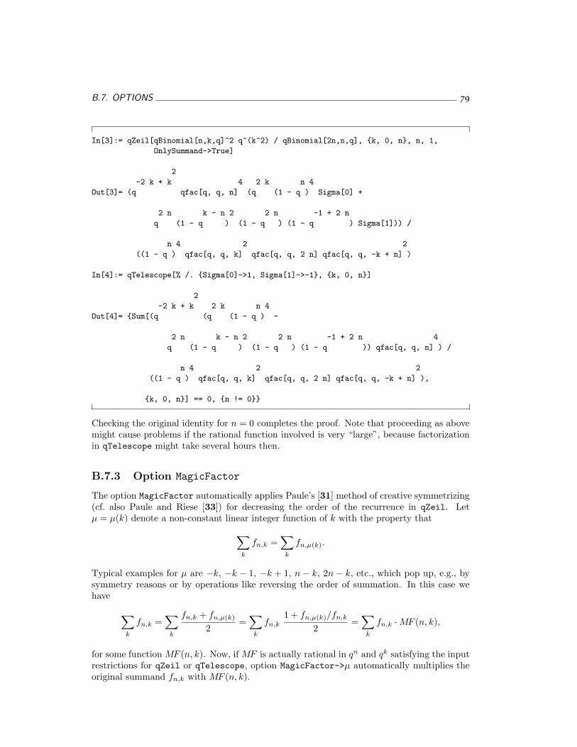
B.7. OPTIONS 79
In[3]:= qZeil[qBinomial[n,k,q]^2 q^(k^2) / qBinomial[2n,n,q], {k, 0, n}, n, 1,
OnlySummand->True]
2
-2 k + k 4 2 k n 4
Out[3]= (q qfac[q, q, n] (q (1 - q ) Sigma[0] +
2 n k - n 2 2 n -1 + 2 n
q (1 - q ) (1 - q ) (1 - q ) Sigma[1])) /
n 4 2 2
((1 - q ) qfac[q, q, k] qfac[q, q, 2 n] qfac[q, q, -k + n] )
In[4]:= qTelescope[% /. {Sigma[0]->1, Sigma[1]->-1}, {k, 0, n}]
2
-2 k + k 2 k n 4
Out[4]= {Sum[(q (q (1 - q ) -
2 n k - n 2 2 n -1 + 2 n 4
q (1 - q ) (1 - q ) (1 - q )) qfac[q, q, n] ) /
n 4 2 2
((1 - q ) qfac[q, q, k] qfac[q, q, 2 n] qfac[q, q, -k + n] ),
{k, 0, n}] == 0, {n != 0}}
Checking the original identity for n = 0 completes the proof. Note that proceeding as abovemight cause problems if the rational function involved is very “large”, because factorizationin qTelescope might take several hours then.
B.7.3 Option MagicFactor
The option MagicFactor automatically applies Paule’s [31] method of creative symmetrizing(cf. also Paule and Riese [33]) for decreasing the order of the recurrence in qZeil. Letµ = µ(k) denote a non-constant linear integer function of k with the property that
∑
k
fn,k =∑
k
fn,µ(k).
Typical examples for µ are −k, −k − 1, −k + 1, n − k, 2n − k, etc., which pop up, e.g., bysymmetry reasons or by operations like reversing the order of summation. In this case wehave
∑
k
fn,k =∑
k
fn,k + fn,µ(k)
2=
∑
k
fn,k
1 + fn,µ(k)/fn,k
2=
∑
k
fn,k ·MF (n, k),
for some function MF (n, k). Now, if MF is actually rational in qn and qk satisfying the inputrestrictions for qZeil or qTelescope, option MagicFactor->µ automatically multiplies theoriginal summand fn,k with MF (n, k).
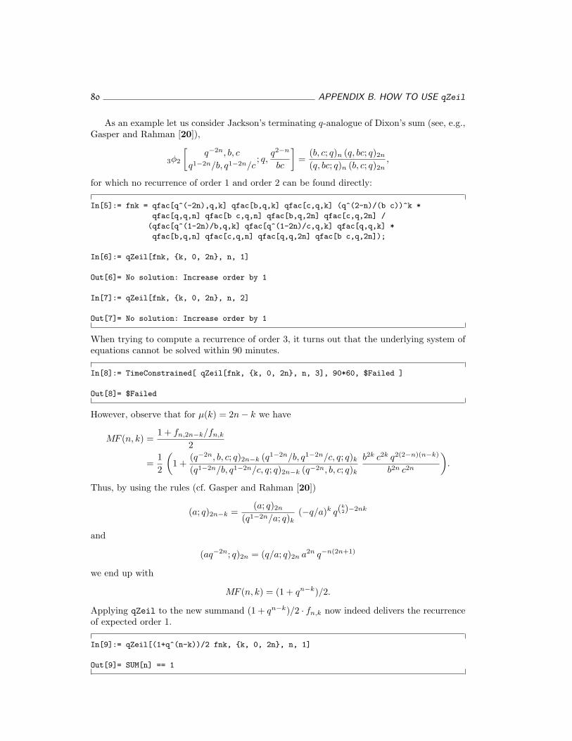
80 APPENDIX B. HOW TO USE qZeil
As an example let us consider Jackson’s terminating q-analogue of Dixon’s sum (see, e.g.,Gasper and Rahman [20]),
3φ2
[q−2n, b, c
q1−2n/b, q1−2n/c; q,
q2−n
bc
]=
(b, c; q)n (q, bc; q)2n
(q, bc; q)n (b, c; q)2n,
for which no recurrence of order 1 and order 2 can be found directly:
In[5]:= fnk = qfac[q^(-2n),q,k] qfac[b,q,k] qfac[c,q,k] (q^(2-n)/(b c))^k *
qfac[q,q,n] qfac[b c,q,n] qfac[b,q,2n] qfac[c,q,2n] /
(qfac[q^(1-2n)/b,q,k] qfac[q^(1-2n)/c,q,k] qfac[q,q,k] *
qfac[b,q,n] qfac[c,q,n] qfac[q,q,2n] qfac[b c,q,2n]);
In[6]:= qZeil[fnk, {k, 0, 2n}, n, 1]
Out[6]= No solution: Increase order by 1
In[7]:= qZeil[fnk, {k, 0, 2n}, n, 2]
Out[7]= No solution: Increase order by 1
When trying to compute a recurrence of order 3, it turns out that the underlying system ofequations cannot be solved within 90 minutes.
In[8]:= TimeConstrained[ qZeil[fnk, {k, 0, 2n}, n, 3], 90*60, $Failed ]
Out[8]= $Failed
However, observe that for µ(k) = 2n− k we have
MF (n, k) =1 + fn,2n−k/fn,k
2
=12
(1 +
(q−2n, b, c; q)2n−k (q1−2n/b, q1−2n/c, q; q)k
(q1−2n/b, q1−2n/c, q; q)2n−k (q−2n, b, c; q)k
b2k c2k q2(2−n)(n−k)
b2n c2n
).
Thus, by using the rules (cf. Gasper and Rahman [20])
(a; q)2n−k =(a; q)2n
(q1−2n/a; q)k(−q/a)k q(
k2)−2nk
and
(aq−2n; q)2n = (q/a; q)2n a2n q−n(2n+1)
we end up with
MF (n, k) = (1 + qn−k)/2.
Applying qZeil to the new summand (1 + qn−k)/2 · fn,k now indeed delivers the recurrenceof expected order 1.
In[9]:= qZeil[(1+q^(n-k))/2 fnk, {k, 0, 2n}, n, 1]
Out[9]= SUM[n] == 1
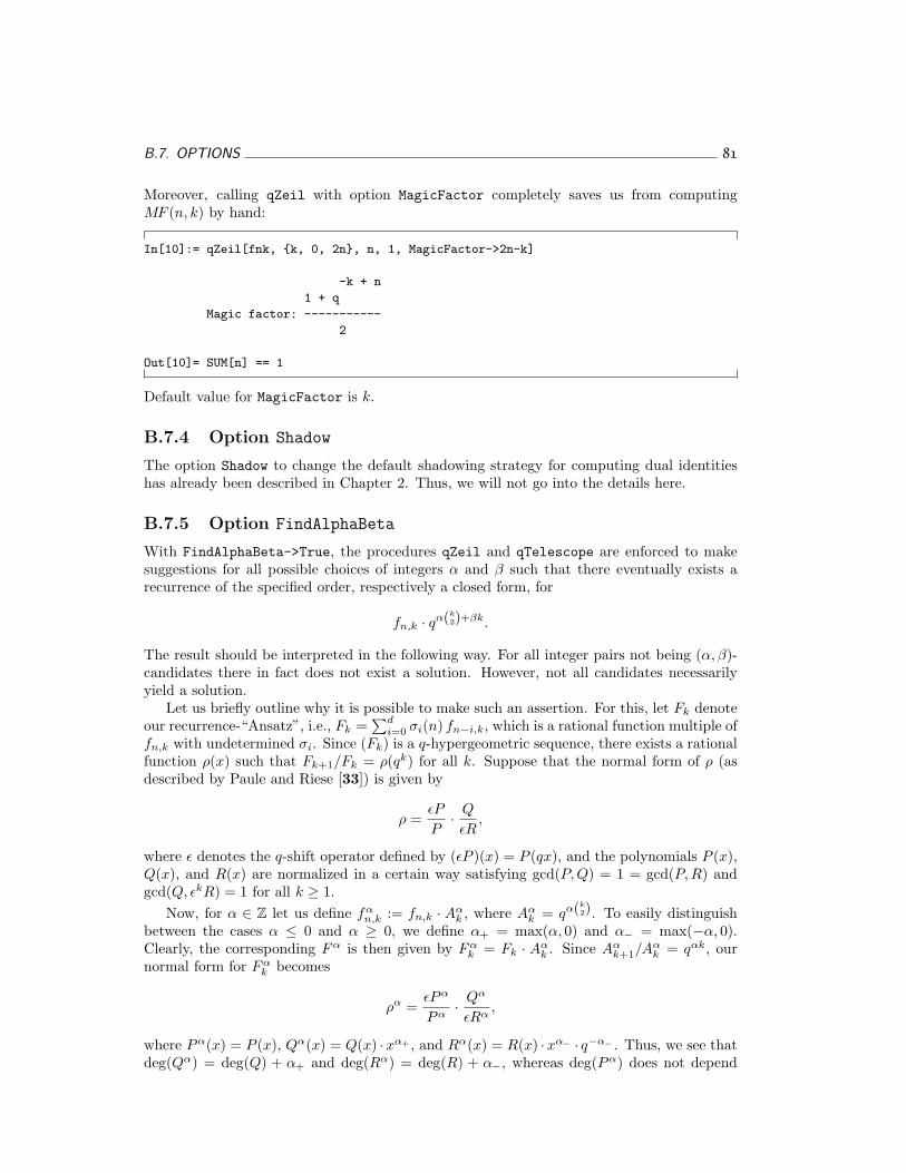
B.7. OPTIONS 81
Moreover, calling qZeil with option MagicFactor completely saves us from computingMF (n, k) by hand:
In[10]:= qZeil[fnk, {k, 0, 2n}, n, 1, MagicFactor->2n-k]
-k + n
1 + q
Magic factor: -----------
2
Out[10]= SUM[n] == 1
Default value for MagicFactor is k.
B.7.4 Option Shadow
The option Shadow to change the default shadowing strategy for computing dual identitieshas already been described in Chapter 2. Thus, we will not go into the details here.
B.7.5 Option FindAlphaBeta
With FindAlphaBeta->True, the procedures qZeil and qTelescope are enforced to makesuggestions for all possible choices of integers α and β such that there eventually exists arecurrence of the specified order, respectively a closed form, for
fn,k · qα(k2)+βk.
The result should be interpreted in the following way. For all integer pairs not being (α, β)-candidates there in fact does not exist a solution. However, not all candidates necessarilyyield a solution.
Let us briefly outline why it is possible to make such an assertion. For this, let Fk denoteour recurrence-“Ansatz”, i.e., Fk =
∑di=0 σi(n) fn−i,k, which is a rational function multiple of
fn,k with undetermined σi. Since (Fk) is a q-hypergeometric sequence, there exists a rationalfunction ρ(x) such that Fk+1/Fk = ρ(qk) for all k. Suppose that the normal form of ρ (asdescribed by Paule and Riese [33]) is given by
ρ =εP
P· Q
εR,
where ε denotes the q-shift operator defined by (εP )(x) = P (qx), and the polynomials P (x),Q(x), and R(x) are normalized in a certain way satisfying gcd(P,Q) = 1 = gcd(P, R) andgcd(Q, εkR) = 1 for all k ≥ 1.
Now, for α ∈ Z let us define fαn,k := fn,k · Aα
k , where Aαk = qα(k
2). To easily distinguishbetween the cases α ≤ 0 and α ≥ 0, we define α+ = max(α, 0) and α− = max(−α, 0).Clearly, the corresponding Fα is then given by Fα
k = Fk · Aαk . Since Aα
k+1/Aαk = qαk, our
normal form for Fαk becomes
ρα =εPα
Pα· Qα
εRα,
where Pα(x) = P (x), Qα(x) = Q(x) ·xα+ , and Rα(x) = R(x) ·xα− · q−α− . Thus, we see thatdeg(Qα) = deg(Q) + α+ and deg(Rα) = deg(R) + α−, whereas deg(Pα) does not depend
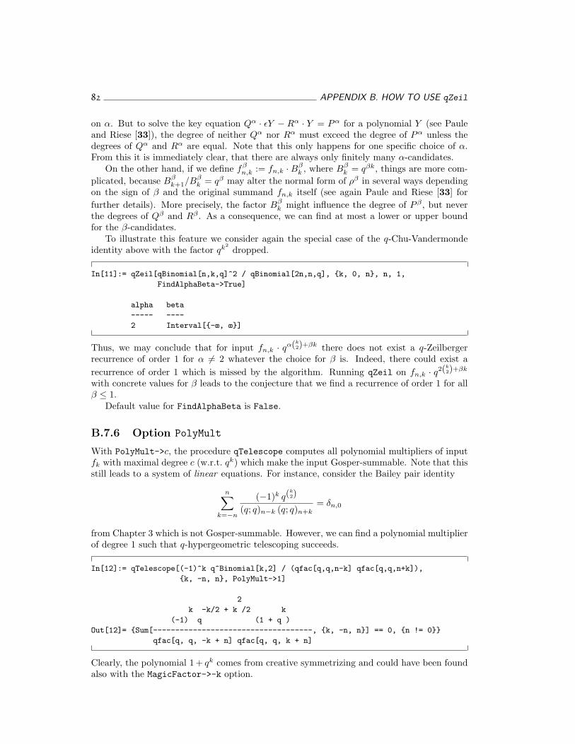
82 APPENDIX B. HOW TO USE qZeil
on α. But to solve the key equation Qα · εY − Rα · Y = Pα for a polynomial Y (see Pauleand Riese [33]), the degree of neither Qα nor Rα must exceed the degree of Pα unless thedegrees of Qα and Rα are equal. Note that this only happens for one specific choice of α.From this it is immediately clear, that there are always only finitely many α-candidates.
On the other hand, if we define fβn,k := fn,k ·Bβ
k , where Bβk = qβk, things are more com-
plicated, because Bβk+1/Bβ
k = qβ may alter the normal form of ρβ in several ways dependingon the sign of β and the original summand fn,k itself (see again Paule and Riese [33] forfurther details). More precisely, the factor Bβ
k might influence the degree of P β , but neverthe degrees of Qβ and Rβ . As a consequence, we can find at most a lower or upper boundfor the β-candidates.
To illustrate this feature we consider again the special case of the q-Chu-Vandermondeidentity above with the factor qk2
dropped.
In[11]:= qZeil[qBinomial[n,k,q]^2 / qBinomial[2n,n,q], {k, 0, n}, n, 1,
FindAlphaBeta−>True]
alpha beta
−−−−− −−−−
2 Interval[{−∞, ∞}]
Thus, we may conclude that for input fn,k · qα(k2)+βk there does not exist a q-Zeilberger
recurrence of order 1 for α 6= 2 whatever the choice for β is. Indeed, there could exist arecurrence of order 1 which is missed by the algorithm. Running qZeil on fn,k · q2(k
2)+βk
with concrete values for β leads to the conjecture that we find a recurrence of order 1 for allβ ≤ 1.
Default value for FindAlphaBeta is False.
B.7.6 Option PolyMult
With PolyMult->c, the procedure qTelescope computes all polynomial multipliers of inputfk with maximal degree c (w.r.t. qk) which make the input Gosper-summable. Note that thisstill leads to a system of linear equations. For instance, consider the Bailey pair identity
n∑
k=−n
(−1)k q(k2)
(q; q)n−k (q; q)n+k= δn,0
from Chapter 3 which is not Gosper-summable. However, we can find a polynomial multiplierof degree 1 such that q-hypergeometric telescoping succeeds.
In[12]:= qTelescope[(-1)^k q^Binomial[k,2] / (qfac[q,q,n-k] qfac[q,q,n+k]),
{k, -n, n}, PolyMult->1]
2
k -k/2 + k /2 k
(-1) q (1 + q )
Out[12]= {Sum[------------------------------------, {k, -n, n}] == 0, {n != 0}}
qfac[q, q, -k + n] qfac[q, q, k + n]
Clearly, the polynomial 1 + qk comes from creative symmetrizing and could have been foundalso with the MagicFactor->-k option.
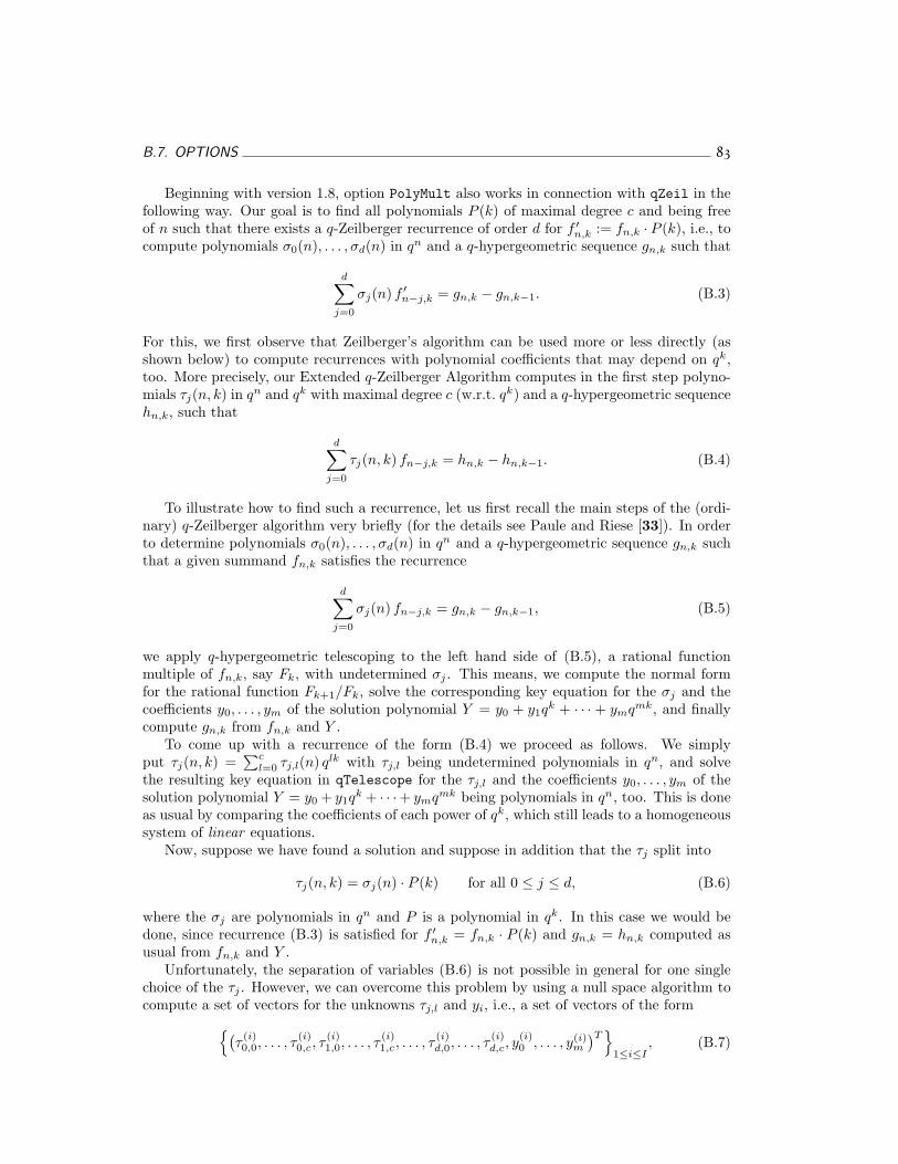
B.7. OPTIONS 83
Beginning with version 1.8, option PolyMult also works in connection with qZeil in thefollowing way. Our goal is to find all polynomials P (k) of maximal degree c and being freeof n such that there exists a q-Zeilberger recurrence of order d for f ′n,k := fn,k · P (k), i.e., tocompute polynomials σ0(n), . . . , σd(n) in qn and a q-hypergeometric sequence gn,k such that
d∑
j=0
σj(n) f ′n−j,k = gn,k − gn,k−1. (B.3)
For this, we first observe that Zeilberger’s algorithm can be used more or less directly (asshown below) to compute recurrences with polynomial coefficients that may depend on qk,too. More precisely, our Extended q-Zeilberger Algorithm computes in the first step polyno-mials τj(n, k) in qn and qk with maximal degree c (w.r.t. qk) and a q-hypergeometric sequencehn,k, such that
d∑
j=0
τj(n, k) fn−j,k = hn,k − hn,k−1. (B.4)
To illustrate how to find such a recurrence, let us first recall the main steps of the (ordi-nary) q-Zeilberger algorithm very briefly (for the details see Paule and Riese [33]). In orderto determine polynomials σ0(n), . . . , σd(n) in qn and a q-hypergeometric sequence gn,k suchthat a given summand fn,k satisfies the recurrence
d∑
j=0
σj(n) fn−j,k = gn,k − gn,k−1, (B.5)
we apply q-hypergeometric telescoping to the left hand side of (B.5), a rational functionmultiple of fn,k, say Fk, with undetermined σj . This means, we compute the normal formfor the rational function Fk+1/Fk, solve the corresponding key equation for the σj and thecoefficients y0, . . . , ym of the solution polynomial Y = y0 + y1q
k + · · · + ymqmk, and finallycompute gn,k from fn,k and Y .
To come up with a recurrence of the form (B.4) we proceed as follows. We simplyput τj(n, k) =
∑cl=0 τj,l(n) qlk with τj,l being undetermined polynomials in qn, and solve
the resulting key equation in qTelescope for the τj,l and the coefficients y0, . . . , ym of thesolution polynomial Y = y0 + y1q
k + · · ·+ ymqmk being polynomials in qn, too. This is doneas usual by comparing the coefficients of each power of qk, which still leads to a homogeneoussystem of linear equations.
Now, suppose we have found a solution and suppose in addition that the τj split into
τj(n, k) = σj(n) · P (k) for all 0 ≤ j ≤ d, (B.6)
where the σj are polynomials in qn and P is a polynomial in qk. In this case we would bedone, since recurrence (B.3) is satisfied for f ′n,k = fn,k · P (k) and gn,k = hn,k computed asusual from fn,k and Y .
Unfortunately, the separation of variables (B.6) is not possible in general for one singlechoice of the τj . However, we can overcome this problem by using a null space algorithm tocompute a set of vectors for the unknowns τj,l and yi, i.e., a set of vectors of the form
{(τ
(i)0,0, . . . , τ
(i)0,c, τ
(i)1,0, . . . , τ
(i)1,c, . . . , τ
(i)d,0, . . . , τ
(i)d,c, y
(i)0 , . . . , y(i)
m
)T}
1≤i≤I, (B.7)
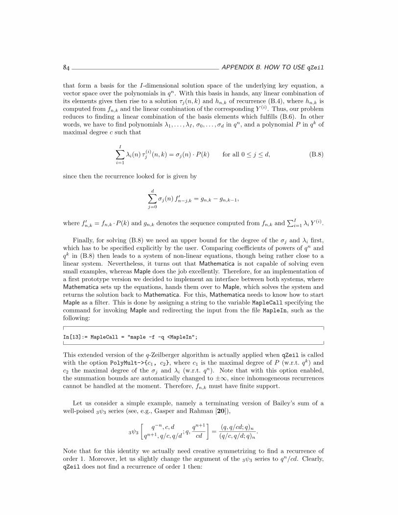
84 APPENDIX B. HOW TO USE qZeil
that form a basis for the I-dimensional solution space of the underlying key equation, avector space over the polynomials in qn. With this basis in hands, any linear combination ofits elements gives then rise to a solution τj(n, k) and hn,k of recurrence (B.4), where hn,k iscomputed from fn,k and the linear combination of the corresponding Y (i). Thus, our problemreduces to finding a linear combination of the basis elements which fulfills (B.6). In otherwords, we have to find polynomials λ1, . . . , λI , σ0, . . . , σd in qn, and a polynomial P in qk ofmaximal degree c such that
I∑
i=1
λi(n) τ(i)j (n, k) = σj(n) · P (k) for all 0 ≤ j ≤ d, (B.8)
since then the recurrence looked for is given by
d∑
j=0
σj(n) f ′n−j,k = gn,k − gn,k−1,
where f ′n,k = fn,k ·P (k) and gn,k denotes the sequence computed from fn,k and∑I
i=1 λi Y (i).
Finally, for solving (B.8) we need an upper bound for the degree of the σj and λi first,which has to be specified explicitly by the user. Comparing coefficients of powers of qn andqk in (B.8) then leads to a system of non-linear equations, though being rather close to alinear system. Nevertheless, it turns out that Mathematica is not capable of solving evensmall examples, whereas Maple does the job excellently. Therefore, for an implementation ofa first prototype version we decided to implement an interface between both systems, whereMathematica sets up the equations, hands them over to Maple, which solves the system andreturns the solution back to Mathematica. For this, Mathematica needs to know how to startMaple as a filter. This is done by assigning a string to the variable MapleCall specifying thecommand for invoking Maple and redirecting the input from the file MapleIn, such as thefollowing:
In[13]:= MapleCall = "maple -f -q <MapleIn";
This extended version of the q-Zeilberger algorithm is actually applied when qZeil is calledwith the option PolyMult->{c1, c2}, where c1 is the maximal degree of P (w.r.t. qk) andc2 the maximal degree of the σj and λi (w.r.t. qn). Note that with this option enabled,the summation bounds are automatically changed to ±∞, since inhomogeneous recurrencescannot be handled at the moment. Therefore, fn,k must have finite support.
Let us consider a simple example, namely a terminating version of Bailey’s sum of awell-poised 3ψ3 series (see, e.g., Gasper and Rahman [20]),
3ψ3
[q−n, c, d
qn+1, q/c, q/d; q,
qn+1
cd
]=
(q, q/cd; q)n
(q/c, q/d; q)n.
Note that for this identity we actually need creative symmetrizing to find a recurrence oforder 1. Moreover, let us slightly change the argument of the 3ψ3 series to qn/cd. Clearly,qZeil does not find a recurrence of order 1 then:
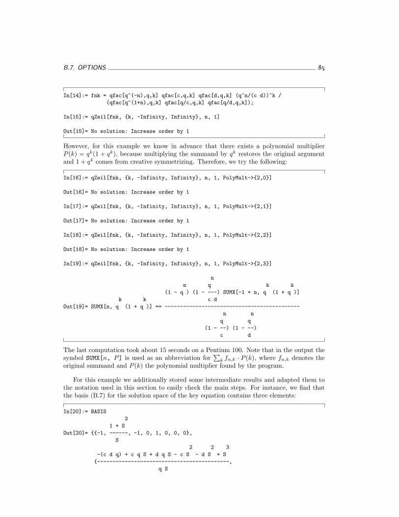
B.7. OPTIONS 85
In[14]:= fnk = qfac[q^(-n),q,k] qfac[c,q,k] qfac[d,q,k] (q^n/(c d))^k /
(qfac[q^(1+n),q,k] qfac[q/c,q,k] qfac[q/d,q,k]);
In[15]:= qZeil[fnk, {k, -Infinity, Infinity}, n, 1]
Out[15]= No solution: Increase order by 1
However, for this example we know in advance that there exists a polynomial multiplierP (k) = qk(1 + qk), because multiplying the summand by qk restores the original argumentand 1 + qk comes from creative symmetrizing. Therefore, we try the following:
In[16]:= qZeil[fnk, {k, -Infinity, Infinity}, n, 1, PolyMult->{2,0}]
Out[16]= No solution: Increase order by 1
In[17]:= qZeil[fnk, {k, -Infinity, Infinity}, n, 1, PolyMult->{2,1}]
Out[17]= No solution: Increase order by 1
In[18]:= qZeil[fnk, {k, -Infinity, Infinity}, n, 1, PolyMult->{2,2}]
Out[18]= No solution: Increase order by 1
In[19]:= qZeil[fnk, {k, -Infinity, Infinity}, n, 1, PolyMult->{2,3}]
n
n q k k
(1 - q ) (1 - ---) SUMX[-1 + n, q (1 + q )]
k k c d
Out[19]= SUMX[n, q (1 + q )] == --------------------------------------------
n n
q q
(1 - --) (1 - --)
c d
The last computation took about 15 seconds on a Pentium 100. Note that in the output thesymbol SUMX[n, P] is used as an abbreviation for
∑k fn,k · P (k), where fn,k denotes the
original summand and P (k) the polynomial multiplier found by the program.
For this example we additionally stored some intermediate results and adapted them tothe notation used in this section to easily check the main steps. For instance, we find thatthe basis (B.7) for the solution space of the key equation contains three elements:
In[20]:= BASIS
2
1 + S
Out[20]= {{-1, ------, -1, 0, 1, 0, 0, 0},
S
2 2 3
-(c d q) + c q S + d q S - c S - d S + S
{-------------------------------------------,
q S
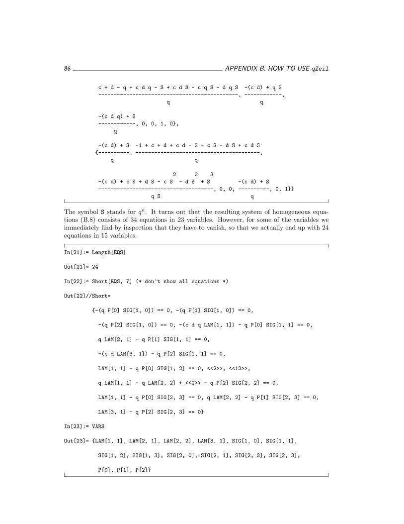
86 APPENDIX B. HOW TO USE qZeil
c + d - q + c d q - S + c d S - c q S - d q S -(c d) + q S
---------------------------------------------, ------------,
q q
-(c d q) + S
------------, 0, 0, 1, 0},
q
-(c d) + S -1 + c + d + c d - S - c S - d S + c d S
{----------, ----------------------------------------,
q q
2 2 3
-(c d) + c S + d S - c S - d S + S -(c d) + S
-------------------------------------, 0, 0, ----------, 0, 1}}
q S q
The symbol S stands for qn. It turns out that the resulting system of homogeneous equa-tions (B.8) consists of 34 equations in 23 variables. However, for some of the variables weimmediately find by inspection that they have to vanish, so that we actually end up with 24equations in 15 variables:
In[21]:= Length[EQS]
Out[21]= 24
In[22]:= Short[EQS, 7] (* don’t show all equations *)
Out[22]//Short=
{-(q P[0] SIG[1, 0]) == 0, -(q P[1] SIG[1, 0]) == 0,
-(q P[2] SIG[1, 0]) == 0, -(c d q LAM[1, 1]) - q P[0] SIG[1, 1] == 0,
q LAM[2, 1] - q P[1] SIG[1, 1] == 0,
-(c d LAM[3, 1]) - q P[2] SIG[1, 1] == 0,
LAM[1, 1] - q P[0] SIG[1, 2] == 0, <<2>>, <<12>>,
q LAM[1, 1] - q LAM[2, 2] + <<2>> - q P[2] SIG[2, 2] == 0,
LAM[1, 1] - q P[0] SIG[2, 3] == 0, q LAM[2, 2] - q P[1] SIG[2, 3] == 0,
LAM[3, 1] - q P[2] SIG[2, 3] == 0}
In[23]:= VARS
Out[23]= {LAM[1, 1], LAM[2, 1], LAM[2, 2], LAM[3, 1], SIG[1, 0], SIG[1, 1],
SIG[1, 2], SIG[1, 3], SIG[2, 0], SIG[2, 1], SIG[2, 2], SIG[2, 3],
P[0], P[1], P[2]}
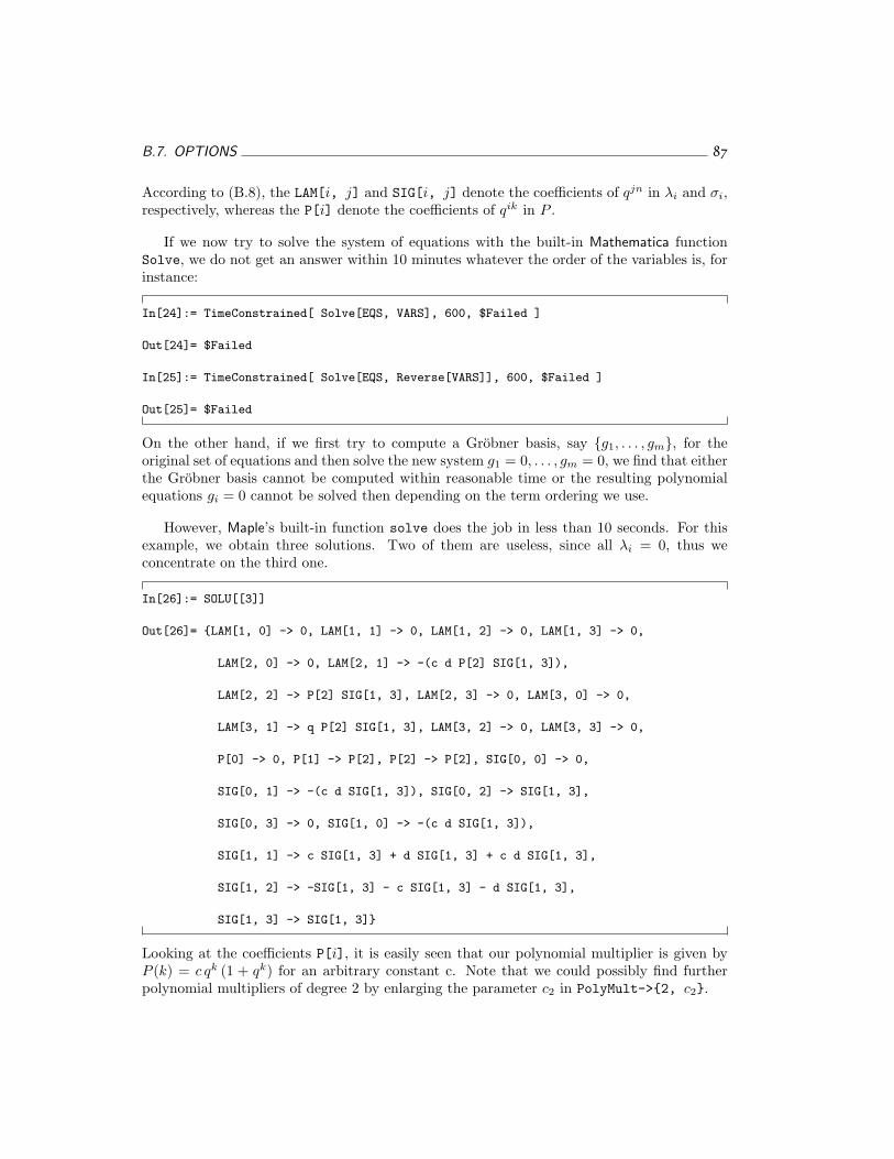
B.7. OPTIONS 87
According to (B.8), the LAM[i, j] and SIG[i, j] denote the coefficients of qjn in λi and σi,respectively, whereas the P[i] denote the coefficients of qik in P .
If we now try to solve the system of equations with the built-in Mathematica functionSolve, we do not get an answer within 10 minutes whatever the order of the variables is, forinstance:
In[24]:= TimeConstrained[ Solve[EQS, VARS], 600, $Failed ]
Out[24]= $Failed
In[25]:= TimeConstrained[ Solve[EQS, Reverse[VARS]], 600, $Failed ]
Out[25]= $Failed
On the other hand, if we first try to compute a Grobner basis, say {g1, . . . , gm}, for theoriginal set of equations and then solve the new system g1 = 0, . . . , gm = 0, we find that eitherthe Grobner basis cannot be computed within reasonable time or the resulting polynomialequations gi = 0 cannot be solved then depending on the term ordering we use.
However, Maple’s built-in function solve does the job in less than 10 seconds. For thisexample, we obtain three solutions. Two of them are useless, since all λi = 0, thus weconcentrate on the third one.
In[26]:= SOLU[[3]]
Out[26]= {LAM[1, 0] -> 0, LAM[1, 1] -> 0, LAM[1, 2] -> 0, LAM[1, 3] -> 0,
LAM[2, 0] -> 0, LAM[2, 1] -> -(c d P[2] SIG[1, 3]),
LAM[2, 2] -> P[2] SIG[1, 3], LAM[2, 3] -> 0, LAM[3, 0] -> 0,
LAM[3, 1] -> q P[2] SIG[1, 3], LAM[3, 2] -> 0, LAM[3, 3] -> 0,
P[0] -> 0, P[1] -> P[2], P[2] -> P[2], SIG[0, 0] -> 0,
SIG[0, 1] -> -(c d SIG[1, 3]), SIG[0, 2] -> SIG[1, 3],
SIG[0, 3] -> 0, SIG[1, 0] -> -(c d SIG[1, 3]),
SIG[1, 1] -> c SIG[1, 3] + d SIG[1, 3] + c d SIG[1, 3],
SIG[1, 2] -> -SIG[1, 3] - c SIG[1, 3] - d SIG[1, 3],
SIG[1, 3] -> SIG[1, 3]}
Looking at the coefficients P[i], it is easily seen that our polynomial multiplier is given byP (k) = c qk (1 + qk) for an arbitrary constant c. Note that we could possibly find furtherpolynomial multipliers of degree 2 by enlarging the parameter c2 in PolyMult->{2, c2}.
88 APPENDIX B. HOW TO USE qZeil
B.8 Additional Functions
The qZeil package comes with its own simplification procedure
qSimplify[exp]
for q-hypergeometric expressions exp. To make this highly non-trivial task powerful andefficient, our strategy is based on collecting several rewrite rules into blocks which are appliedone after the other. Furthermore, note that this procedure does not factor at all.
In the context of qWZ-dualization (see Chapter 2), after a dual pair (f ′n,k, g′n,k) has beencomputed by the program, calling
DualId[{k, a, b}, n]
evaluates SUM ′(n) :=∑b
k=a f ′n,k provided that SUM ′ is constant, i.e., not depending on n.DualId uses the value of the (global) variable DualPair.
The functionSameRec[rec1, rec2]
checks whether the recurrences rec1 and rec2 are equal. This is useful and very fast for higher-order recurrences arising from transformation formulas which quite frequently yield severalpages of output. In this case, SameQ does not necessarily give True for equal recurrences andTogether[ rec1[[2]] - rec2[[2]] ] can be rather time-consuming. Similarly, the function
Check1[rec]
checks whether the recurrence rec is satisfied by 1.
Finally,ToqHyper[rec]
converts the recurrence rec into valid input for Petkovsek’s package qHyper (see Abramov,Paule, and Petkovsek [1]) in terms of SUM(S) := SUM(qn). Since both packages qHyperand qZeil define the symbol q, one has to set the global variable NoContext to True and toreload the packages which will then reside in context Global‘. This is an inelegant but veryuseful hack allowing the simultaneous use of different packages defining the same symbolsprovided that the packages do not define functions with the same name and the same numberof arguments. Note that the original behavior can be restored only by restarting Mathematica.
B.9 Speed-Up
With the latest version of qZeil we could achieve a significant speed-up mainly based ontwo new ideas, an improved pivot search in Aichinger’s [3] null space algorithm and a newpreprocessing of the recurrence looked for. As a consequence we can now, for instance,compute a recurrence of order 3 for the 12φ11 series on the right hand side of identity (III.25)in Gasper and Rahman [20] within less than one minute (this was the “out-of-memory”example listed in Paule and Riese [33]).
The new pivot search method is based on the observation that not only the size of thepivot element plays a fundamental role in Gaussian elimination but also the number of zerosin the corresponding row. Note that whenever we speak of the “size” of a rational function weactually mean its “complexity” which in the present implementation is determined with the
B.9. SPEED-UP 89
Mathematica function LeafCount. Thus we first look for the rows of the underlying matrixM for which the number of zeros is maximal. Let RM = {r1, . . . , rd} denote the set of thoserows. If RM consists of only one element, we simply choose the smallest non-zero entry ofrow r1 as our pivot element. Otherwise, it is obvious that the effectiveness of our methodheavily depends also on the total size of the ri from which the pivot element is chosen. Letsi and ti denote the size of the smallest non-zero entry of ri, respectively the total size of ri.A natural way to decide that the pivot element should be the smallest non-zero element ofrn instead of rm is when
( sn
sm
)c
<tmtn
for some positive number c. It turns out that — at least for matrices appearing in q-hyper-geometric summation — the choice c = 3/4 leads to highly satisfactory results. Additionalevidence for our improvement of efficiency stems from the fact that this kind of pivot searchhas been also successfully integrated into Wegschaider’s [42] package MultiSum for auto-matically proving binomial multi-sum identities resulting in a speed-up factor of 10 there.Moreover, the approach described above could be improved once more by taking the numberof zeros in the columns into account, too.
The second idea which substantially helped to decrease the run-time, simply consists infiltering out all factors not depending on qk in the polynomials pi(n, k) of the recurrence-“Ansatz”
d∑
i=0
σi(n) fn−i,k = fn,k · σ0(n) p0(n, k) + σ1(n) p1(n, k) + · · ·+ σd(n) pd(n, k)pd+1(n, k)
.
Those constant factors only blow up the system of equations unnecessarily. It is sufficient totake them into consideration after the system of equations has been solved.

90
91
Bibliography
[1] S.A. Abramov, P. Paule, and M. Petkovsek, q-Hypergeometric solutions of q-difference equations, to appear in Discrete Mathematics.
[2] A.K. Agarwal, G.E. Andrews, and D.M. Bressoud, The Bailey lattice, J. IndianMath. Soc., 51 (1987), pp. 57–73.
[3] E. Aichinger, A linear system solver for Mathematica that uses SACLIB (Version 1.0),Technical Report 97–05, RISC, J. Kepler University, Linz, Austria, February 1997.
[4] W. Al-Salam and A. Verma, On quadratic transformations of basic series, SIAM J.Math. Anal., 15 (1984), pp. 414–421.
[5] G.E. Andrews, On basic hypergeometric series, mock-theta-functions and parti-tions (II), Quart. J. Math. Oxford (2), 17 (1966), pp. 132–143.
[6] , Number Theory, W.B. Saunders, Philadelphia, 1971. (Reprinted: HindustanPublishing Co., New Delhi, 1984.)
[7] , The Theory of Partitions, Encyclopedia of Mathematics and Its Appl., Vol. 2,Addison-Wesley, Reading, 1976. (Reissued: Cambridge University Press, London andNew York, 1985.)
[8] , Connection coefficient problems and partitions, Proc. Symp. Pure Math.,Vol. 34, pp. 1–24, Amer. Math. Soc., Providence, 1979.
[9] , Multiple series Rogers-Ramanujan type identities, Pacific J. Math., 114 (1984),pp. 267–283.
[10] , q-Series: Their Development and Application in Analysis, Number Theory,Combinatorics, Physics, and Computer Algebra, CBMS Regional Conference Series,No. 66, Amer. Math. Soc., Providence, 1986.
[11] G.E. Andrews and D. Hickerson, Ramanujan’s “lost” notebook VII: The sixth ordermock theta functions, Adv. in Math., 89 (1991), pp. 60–105.
[12] R. Askey, The q-gamma and q-beta functions, Appl. Anal., 8 (1978), pp. 125–141.
[13] W.N. Bailey, Generalized Hypergeometric Series, Cambridge Math. Tract, No. 32,Cambridge University Press, Cambridge, 1935. (Reprinted: Hafner, New York, 1964.)
[14] , Some identities in combinatory analysis, Proc. London Math. Soc. (2), 49(1947), pp. 421–435.
92 BIBLIOGRAPHY
[15] , Identities of the Rogers-Ramanujan type, Proc. London Math. Soc. (2), 50(1949), pp. 1–10.
[16] A. Bauer and M. Petkovsek, Multibasic and mixed Gosper’s algorithm, Preprint.
[17] D.M. Bressoud, The Bailey lattice: an introduction, in “Ramanujan Revisited” (G.E.Andrews et al., eds.), pp. 57–67, Academic Press, New York, 1988.
[18] L. Carlitz, Some formulas of F.H. Jackson, Monatsh. Math., 73 (1969), pp. 193–198.
[19] G. Gasper, Summation, transformation, and expansion formulas for bibasic series,Trans. Amer. Math. Soc., 312 (1989), pp. 257–277.
[20] G. Gasper and M. Rahman, Basic Hypergeometric Series, Encyclopedia of Mathe-matics and Its Appl., Vol. 35, Cambridge University Press, London and New York,1990.
[21] , An indefinite bibasic summation formula and some quadratic, cubic, and quarticsummation and transformation formulas, Canad. J. Math., 42 (1990), pp. 1–27.
[22] I.M. Gessel, Finding identities with the WZ method, J. Symbolic Computation, 20(1995), pp. 537–566.
[23] I.M. Gessel and D. Stanton, Applications of q-Lagrange inversion to basic hyper-geometric series, Trans. Amer. Math. Soc., 277 (1983), pp. 173–201.
[24] R.W. Gosper, Decision procedures for indefinite hypergeometric summation, Proc.Natl. Acad. Sci. U.S.A., 75 (1978), pp. 40–42.
[25] T.H. Koornwinder, On Zeilberger’s algorithm and its q-analogue, J. Comput. Appl.Math., 48 (1993), pp. 91–111.
[26] C. Krattenthaler, Personal communication, August 1997.
[27] P. Paule, Zwei neue Transformationen als elementare Anwendungen der q-Vander-monde Formel, Ph.D. thesis, University of Vienna, Austria, 1982.
[28] , On identities of the Rogers-Ramanujan type, J. Math. Anal. Appl., 107 (1985),pp. 255–284.
[29] , A note on Bailey’s lemma, J. Comb. Th. (A), 44 (1987), pp. 164–167.
[30] , The concept of Bailey chains, Actes du Seminaire Lotharingien, Vol. 18, pp. 53–76, IRMA Strasbourg, 1988.
[31] , Short and easy computer proofs of the Rogers-Ramanujan identities and ofidentities of similar type, Electr. J. Comb., 1 (1994), #R10.
[32] , Greatest factorial factorization and symbolic summation, J. Symbolic Compu-tation, 20 (1995), pp. 235–268.
[33] P. Paule and A. Riese, A Mathematica q-analogue of Zeilberger’s algorithmbased on an algebraically motivated approach to q-hypergeometric telescoping, in“Special Functions, q-Series and Related Topics” (M.E.H. Ismail, D.R. Masson,and M. Rahman, eds.), Fields Institute Communications, Vol. 14, pp. 179–210,Amer. Math. Soc., Providence, 1997.
BIBLIOGRAPHY 93
[34] P. Paule and V. Strehl, Symbolic summation — some recent developments, in“Computeralgebra in Science and Engineering — Algorithms, Systems, Applica-tions” (J. Fleischer et al., eds.), pp. 138–162, World Scientific, Singapore, 1995.
[35] M. Petkovsek, Hypergeometric solutions of linear recurrences with polynomial coeffi-cients, J. Symbolic Computation, 14 (1992), pp. 243–264.
[36] M. Petkovsek, H.S. Wilf, and D. Zeilberger, A = B, A.K. Peters, Wellesley,1996.
[37] A. Riese, A Mathematica q-analogue of Zeilberger’s algorithm for proving q-hypergeo-metric identities, Diploma thesis, RISC, J. Kepler University, Linz, Austria, 1995.
[38] , A generalization of Gosper’s algorithm to bibasic hypergeometric summation,Electr. J. Comb., 3 (1996), #R19.
[39] L.J. Slater, A new proof of Rogers’s transformations of infinite series, Proc. LondonMath. Soc. (2), 53 (1951), pp. 460–475.
[40] , Further identities of the Rogers-Ramanujan type, Proc. London Math. Soc. (2),54 (1952), pp. 147–167.
[41] , Generalized Hypergeometric Functions, Cambridge University Press, Cam-bridge, 1966.
[42] K. Wegschaider, Computer generated proofs of binomial multi-sum identities, Di-ploma thesis, RISC, J. Kepler University, Linz, Austria, 1997.
[43] H.S. Wilf, Identities and their computer proofs, “SPICE” lecture notes, available inelectronic form via anonymous ftp of the file pub/wilf/lecnotes.ps at the siteftp.cis.upenn.edu, 1993.
[44] H.S. Wilf and D. Zeilberger, Rational functions certify combinatorial identities,J. Amer. Math. Soc., 3 (1990), pp. 147–158.
[45] , An algorithmic proof theory for hypergeometric (ordinary and “q”) multi-sum/integral identities, Invent. Math., 108 (1992), pp. 575–633.
[46] D. Zeilberger, A fast algorithm for proving terminating hypergeometric identities,Discrete Math., 80 (1990), pp. 207–211.
[47] , A holonomic systems approach to special functions identities, J. Comput. Appl.Math., 32 (1990), pp. 321–368.
[48] , The method of creative telescoping, J. Symbolic Computation, 11 (1991),pp. 195–204.
[49] , Three recitations on holonomic systems and hypergeometric series, J. SymbolicComputation, 20 (1995), pp. 699–724.

94
VITA 95
Axel Riese
Research Institute for Symbolic Computation (RISC)Johannes Kepler University, A–4040 Linz, Austria
tel: +43 (0)732 2468-9981 fax: +43 (0)732 [email protected]
http://www.risc.uni-linz.ac.at/research/combinat/risc
Date and Place of Birth: February 4, 1971, Linz
Nationality: Austria
Home Address: Haerdtlstraße 8, A–4040 Linz, Austria
Education:
1977 – 1981 Primary School, VS 30, Linz1981 – 1989 High School, BG Ramsauerstraße, Linz1989 – 1995 Studies in “Technische Mathematik, Studienzweig Informations- und
Datenverarbeitung” at J. Kepler University, Linz1995 Diploma degree1995 – Ph.D. study at Research Institute for Symbolic Computation, J. Kepler
University, Linz
Publications:
A. Riese, A Mathematica q-analogue of Zeilberger’s algorithm for proving q-hypergeo-metric identities, Diploma thesis, RISC, J. Kepler University Linz, 1995.
A. Riese, A generalization of Gosper’s algorithm to bibasic hypergeometric summation,Electr. J. Comb., 3 (1996), #R19.
P. Paule and A. Riese, A Mathematica q-Analogue of Zeilberger’s Algorithm Basedon an Algebraically Motivated Approach to q-Hypergeometric Telescoping, in “SpecialFunctions, q-Series and Related Topics” (M.E.H. Ismail, D.R. Masson, and M. Rahman,eds.), Fields Institute Communications, Vol. 14, pp. 179–210, 1997.

![HYPERGEOMETRIC FUNCTIONS IarXiv:1309.4568v1 [math.CA] 18 Sep 2013 HYPERGEOMETRIC FUNCTIONS I IAN G. MACDONALD Contents Foreword 1 1. 2 2. Particular cases 4 3. Integral formulae 7](https://img.pdfslide.tips/doc/110x75/5e2f371461b5076fc4686c08/hypergeometric-functions-i-arxiv13094568v1-mathca-18-sep-2013-hypergeometric.jpg)