Embed Size (px)
Citation preview
MINISTÈRE DE L'ENSEIGNEMENT SUPÉRIEUR ET DE LA RECHERCHE
******
INSTITUT NATIONAL DES SCIENCES APPLIQUÉES
TOULOUSE
Département de Génie Électrique & Informatique
******
PROJET DE FIN D’ÉTUDES
CONTROL OF A MINI UNMANNEDAERIAL VEHICULE
LATTIS - Toulouse
PRUVOST Côme5 TRS - AE
Juin 2009


Acknowledgments
M. ACCO Pascal Training supervisorM. AURIOL Guillaume Supervisor concerning the SysML part
Mme FOURNIER Danièle LATTIS DirectorM. TONDU Bertrand Referral agent at INSA
M. MAHOUT Vincent Year coordinator for 5 TRS

TABLE OF CONTENTS vii
Table of Contents
1 Presentation 31.1 The Mini Unmanned Aerial Vehicles . . . . . . . . . . . . . . . . . . 31.2 System engineering in automatic control . . . . . . . . . . . . . . . 4
2 Existing methods for system engineering 52.1 About top-down and bottom-up . . . . . . . . . . . . . . . . . . . . . 52.2 Introduction to UML/SysML . . . . . . . . . . . . . . . . . . . . . . . 62.3 Introduction to the SYSMOD approach . . . . . . . . . . . . . . . . 82.4 The new method . . . . . . . . . . . . . . . . . . . . . . . . . . . . . . . 11
3 The product model 133.1 The background . . . . . . . . . . . . . . . . . . . . . . . . . . . . . . . 133.2 The project context . . . . . . . . . . . . . . . . . . . . . . . . . . . . . 143.3 First level requirements . . . . . . . . . . . . . . . . . . . . . . . . . . . 143.4 The system context . . . . . . . . . . . . . . . . . . . . . . . . . . . . . 163.5 The use cases . . . . . . . . . . . . . . . . . . . . . . . . . . . . . . . . . . 16
4 The non linear model 194.1 Mechanical bases used . . . . . . . . . . . . . . . . . . . . . . . . . . . . 194.2 Non linear equations . . . . . . . . . . . . . . . . . . . . . . . . . . . . 204.3 Simulink® model . . . . . . . . . . . . . . . . . . . . . . . . . . . . . . . 22
5 Fixed point computation 235.1 The engines . . . . . . . . . . . . . . . . . . . . . . . . . . . . . . . . . . 235.2 Orientation . . . . . . . . . . . . . . . . . . . . . . . . . . . . . . . . . . 245.3 Position . . . . . . . . . . . . . . . . . . . . . . . . . . . . . . . . . . . . . 255.4 Application to the four engines MUAV . . . . . . . . . . . . . . . . 265.5 Note about holonomy . . . . . . . . . . . . . . . . . . . . . . . . . . . 275.6 Study of a 3 engines MUAV . . . . . . . . . . . . . . . . . . . . . . . . 28
6 Linearisation of system model 316.1 About the linearisation process . . . . . . . . . . . . . . . . . . . . . . 316.2 The engines . . . . . . . . . . . . . . . . . . . . . . . . . . . . . . . . . . 326.3 Acceleration, velocity, position . . . . . . . . . . . . . . . . . . . . . . 346.4 Orientation . . . . . . . . . . . . . . . . . . . . . . . . . . . . . . . . . . 356.5 Final state space . . . . . . . . . . . . . . . . . . . . . . . . . . . . . . . . 41
viii CONTROL OF A MINI UNMANNED AERIAL VEHICULE
7 Validation and model feedback 437.1 Validation of the linear model . . . . . . . . . . . . . . . . . . . . . . . 437.2 Observability tests . . . . . . . . . . . . . . . . . . . . . . . . . . . . . . 457.3 Feedback on product model . . . . . . . . . . . . . . . . . . . . . . . . 45
A Simulink® non linear model A1A.1 Overview . . . . . . . . . . . . . . . . . . . . . . . . . . . . . . . . . . . . A1A.2 The engines . . . . . . . . . . . . . . . . . . . . . . . . . . . . . . . . . . A3A.3 Acceleration, velocity, position . . . . . . . . . . . . . . . . . . . . . . A3A.4 Orientation . . . . . . . . . . . . . . . . . . . . . . . . . . . . . . . . . . A3A.5 Details of custom blocks . . . . . . . . . . . . . . . . . . . . . . . . . . A6
B Matlab code A9B.1 Linearised model . . . . . . . . . . . . . . . . . . . . . . . . . . . . . . . A9
C SysML model A17C.1 Packages hierarchy . . . . . . . . . . . . . . . . . . . . . . . . . . . . . . A17C.2 Stakeholders . . . . . . . . . . . . . . . . . . . . . . . . . . . . . . . . . . A18C.3 Requirements . . . . . . . . . . . . . . . . . . . . . . . . . . . . . . . . . A19C.4 Use cases . . . . . . . . . . . . . . . . . . . . . . . . . . . . . . . . . . . . A22C.5 Environment . . . . . . . . . . . . . . . . . . . . . . . . . . . . . . . . . A23C.6 Activity . . . . . . . . . . . . . . . . . . . . . . . . . . . . . . . . . . . . . A24C.7 Component choice . . . . . . . . . . . . . . . . . . . . . . . . . . . . . . A25
Bibliography A27
Credits A28
Lexicon A29
ABSTRACT 1
AbstractI did my internship in the automatic control research laboratory based at theInstitut National des Sciences Appliquées de Toulouse engineer school, the LAbo-ratoire Toulousain de Technologie et d’Ingénierie des Systèmes. The LATTIS holdsprojects on automatic control, electronics, signal processing and system engi-neering. I joined an already started project studying the Mini Unmanned AerialVehicles, that is to say objects that flies with no pilot inside. It differs from radiocontrolled planes by the level of actions the MUAV can do alone.
The goal of the project is to provide a laboratory session targeted to the fifthyear INSA students in the industrial systems orientation 5GSI.The subject wasinitially defined as “Distant control of a mini unmanned aerial vehicle”. Indeed,the project includes several parts of the LATTIS which has different interests inthe project. The MUAV will serve as an illustration of conception methods andconcepts such that “hardware in the loop” or “software in the loop”. Anotherinterest of the LATTIS is to work on system engineering methods and it wasdecided that the project would be a practical test for study of a new systemconception method mixing several other existing methods.
First of all, we will define the interest of using a system engineering methodin an automatic control project. We will consider the methods that already ex-ist with their advantages and drawbacks and state what we expect to introduceor improve in these methods. Starting from the best suitable existing method,we will start modelling our product. Then, we will have a stronger interest inthe automatic control part. This part follows a work already done that will bepresented later and defines the non linear model of a four engines MUAV. Fromthis model, we will compute the fixed points and realise linearisation. Hope-fully, this part will bring some knowledge allowing us to improve and enrichour product model.
Note that words followed by a star* are defined in the lexicon at the end ofthis report.

2 CONTROL OF A MINI UNMANNED AERIAL VEHICULE
Chapter 1Presentation
1.1 The Mini Unmanned Aerial Vehicles
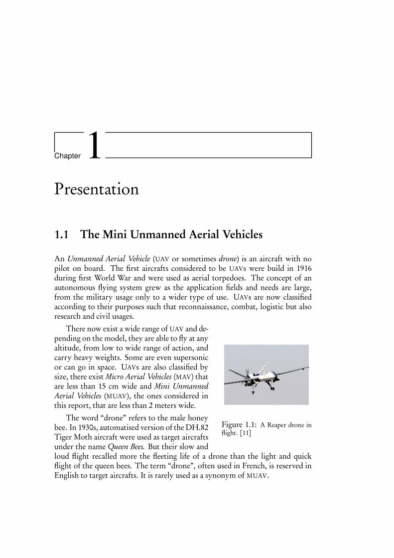
An Unmanned Aerial Vehicle (UAV or sometimes drone) is an aircraft with nopilot on board. The first aircrafts considered to be UAVs were build in 1916during first World War and were used as aerial torpedoes. The concept of anautonomous flying system grew as the application fields and needs are large,from the military usage only to a wider type of use. UAVs are now classifiedaccording to their purposes such that reconnaissance, combat, logistic but alsoresearch and civil usages.
Figure 1.1: A Reaper drone inflight. [11]
There now exist a wide range of UAV and de-pending on the model, they are able to fly at anyaltitude, from low to wide range of action, andcarry heavy weights. Some are even supersonicor can go in space. UAVs are also classified bysize, there exist Micro Aerial Vehicles (MAV) thatare less than 15 cm wide and Mini UnmannedAerial Vehicles (MUAV), the ones considered inthis report, that are less than 2 meters wide.
The word “drone” refers to the male honeybee. In 1930s, automatised version of the DH.82Tiger Moth aircraft were used as target aircraftsunder the name Queen Bees. But their slow andloud flight recalled more the fleeting life of a drone than the light and quickflight of the queen bees. The term “drone”, often used in French, is reserved inEnglish to target aircrafts. It is rarely used as a synonym of MUAV.
4 CONTROL OF A MINI UNMANNED AERIAL VEHICULE
1.2 System engineering in automatic control“Systems engineering is an interdisciplinary field of engineering that focuses on howcomplex engineering projects should be designed and managed.” — Wikipedia[9]
Even for someone familiar with the concept and the practical methods of sys-tem engineering and automatic control, the idea of mixing both can be unclear.System engineering is the art of handling complex projects, defining systemsand their components, managing teams around determined tasks and make surethe final product meets the specifications. On the other hand, automatic con-trol analyses physical processes and tries to make it produce a desired output bytuning its input.
Usually, the two works are separated and often devoted to different teams.Most of the time, the system engineering team will provide the automatic con-trol team with material they have chosen: the system to analyse, the componentsto control and their physical values. Only then, the automatic control team willdecide the adapted controller and do its best so the components behave as ex-pected.
We are convinced that during system analysis done by the automatic controlteam, results can show that the chosen component is not a good one, or that thegoals could be reached more nicely with another one. It may also raise resultsthat would improve or simplify the model, help decision or even raise importantquestions that have to be answered before product is released. This part, oftenforgotten by engineering methods, can be called feedback. It consists in takingnot definitive but temporary decisions during the system engineering process,feed the automatic control with some values and have a feedback to validateor not the decisions. This is only possible provided that automatic control istaken as a whole part of the system engineering process. This report proposesto highlight these facts, show some examples and state preliminary guidelines todeal with this issue.
Chapter 2Existing methods for systemengineering
System engineering is a huge task that is central in any complex project. Thistask can’t be realised correctly without a good knowledge of what is to be done,step by step. Many people devoted time to think about this issue and proposedseveral methods proved to be efficient. They provide step by step guidelines sothe system engineer deals with every aspect of the system as much exhaustivelyas possible.
2.1 About top-down and bottom-up
More than methods, top-down and bottom-up are strategies for dealing with in-formation and knowledge ordering. The greatest part of the methods is build ontop of one of these strategies, like the V-model, the waterfall model, the iterativemodel, the agile model,. . .
The top-down method consists in defining first the most global system, andthen iteratively split and granulates this system into smaller structural functionalparts, that is to say a block that represents a single functionality or structureof the block in the level right above. Step by step, the model gains in detailsand ideally finally defines all aspects of the system. The method allows an easyseparation of higher and lower levels, already defined modules and how they in-tegrate with each other, so work can be easily shared between people and teams.
As an opposite, the bottom-up methodology works as bricks of LEGO®. Onefirst details as much as possible all the most little components one has got tobuild the system and then defines brick by brick the properties of componentsassemblies. The strength of the method is that one always start from what is
6 CONTROL OF A MINI UNMANNED AERIAL VEHICULE
perfectly known so it is sure that the system is finally completely defined and noobscure zone is left, neither at the beginning, nor at the end.
Of course, both methods have their own drawbacks. The top-down methodlacks the insurance that every piece is defined in the conception, and it is diffi-cult to be sure that a functionality will be present because it will be implementedonly at the lowest level, so at the end of the method. As preliminary studies donot care about low level components limitations, when a problem occur, it ismuch more difficult to find the cause and make changes. This is the conclu-sion of an appendix written by Richard Feynman in the report about the spaceshuttle Columbia accident[2].
On the other hand, building a system using bottom-up is hard and hazardousas it requires a big part of intuition to decide what functionality a module willprovide. One is also never insured that the final system will correspond to whatwas expected at first. Obviously, such a method cannot be used alone for aproject following high level only specifications.
2.2 Introduction to UML/SysML
“The OMG Systems Modelling Language (OMG SysML™) is a general-purpose graph-ical modelling language for specifying, analysing, designing, and verifying complexsystems that may include hardware, software, information, personnel, procedures,and facilities.” — The Object Management Group[3]
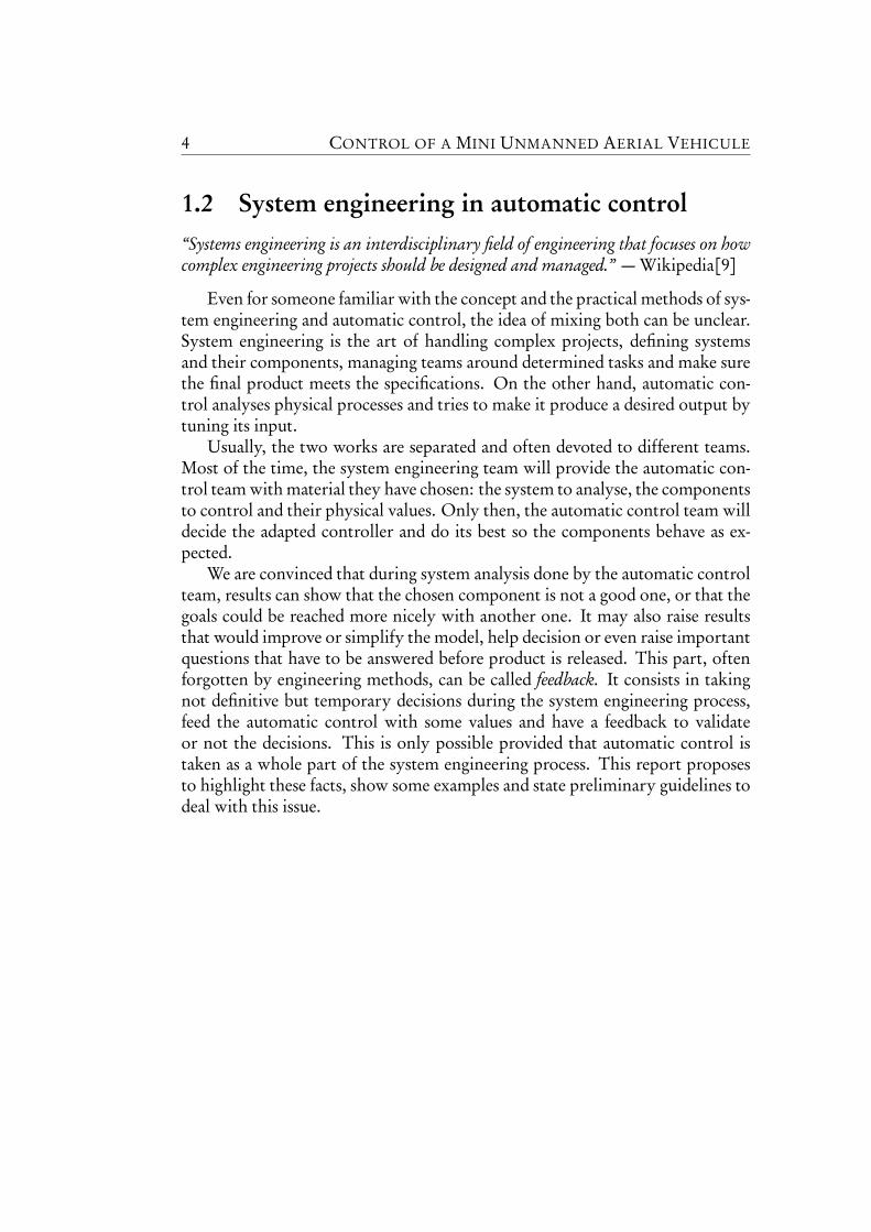
Along with system engineering methods, exist languages used to help thedefinition of the product. They propose a graphical representation of the con-cepts involved in system engineering and their standardisation allows anybodyto understand what is represented. They are not to be confounded with meth-ods, as they do not provide the step by step guidelines to draw the diagrams theysuggest but they provide to such methods a strong framework to write downefficiently the results of their steps.
Figure 2.1: An object diagram inUML. [12]
Commonly, UML* is used in softwareengineering to define complex object ori-ented programs. It defines a set of symbolsused to represent concepts organised in di-agrams, that is to say a space like a pieceof paper where symbols of a special kindare drawn. Unfortunately, place is missingin this report to efficiently introduce UML.The book by Tim Weilkiens[8] devote acomplete chapter to this language. The ar-
EXISTING METHODS FOR SYSTEM ENGINEERING 7
ticle Practical UML: A Hands-On Introduction for Developers[6] also presents ashort but very nice introduction to UML.
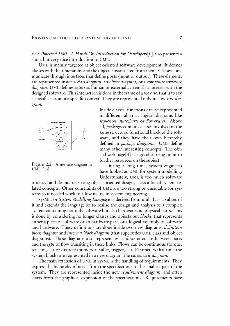
UML is mainly targeted at object oriented software development. It definesclasses with their hierarchy and the objects instantiated from them. Classes com-municate through interfaces that define ports (input or output). These elementsare represented inside a class diagram, an object diagram, or a composite structurediagram. UML defines actors as human or external system that interact with thedesigned software. This interaction is done in the frame of a use case, that is to saya specific action in a specific context. They are represented only in a use case dia-gram.
Figure 2.2: A use case diagram inUML. [13]
Inside classes, functions can be representedin different abstract logical diagrams likesequences, statecharts or flowcharts. Aboveall, packages contains classes involved in thesame structural functional block of the soft-ware, and they have their own hierarchydefined in package diagrams. UML definemany other interesting concepts. The offi-cial web page[4] is a good starting point tofurther resources on the subject.
During a long time, system engineershave looked at UML for system modelling.Unfortunately, UML is too much software
oriented and despite its strong object oriented design, lacks a lot of system re-lated concepts. Other constraints of UML are too strong or unsuitable for sys-tems so it needed work to allow its use in system engineering.
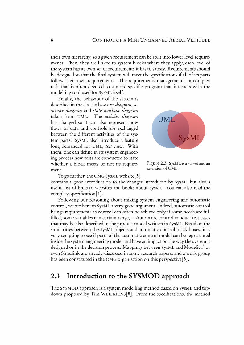
SysML, or System Modelling Language is derived from uml. It is a subset ofit and extends the language so to realise the design and analysis of a complexsystem containing not only software but also hardware and physical parts. Thisis done by considering no longer classes and objects but blocks, that representseither a piece of software or an hardware part, or a logical assembly of softwareand hardware. These definitions are done inside two new diagrams, definitionblock diagram and internal block diagram (that supersedes UML class and objectdiagrams). These diagrams also represent what flows circulate between partsand the type of flow transiting in these links. Flows can be continuous (torque,tension,. . . ) or discrete (numerical value, trigger,. . . ). Parameters that tune thesystem blocks are represented in a new diagram, the parametric diagram.
The main extension of UML in SysML is the handling of requirements. Theyexpress the hierarchy of needs from the specifications to the smallest part of thesystem. They are represented inside the new requirement diagram, and oftenstarts from the graphical expression of the specifications. Requirements have
8 CONTROL OF A MINI UNMANNED AERIAL VEHICULE
their own hierarchy, so a given requirement can be split into lower level require-ments. Then, they are linked to system blocks where they apply, each level ofthe system has its own set of requirements it has to satisfy. Requirements shouldbe designed so that the final system will meet the specifications if all of its partsfollow their own requirements. The requirements management is a complextask that is often devoted to a more specific program that interacts with themodelling tool used for SysML itself.
UML
SysML
Figure 2.3: SysML is a subset and anextension of UML.
Finally, the behaviour of the system isdescribed in the classical use case diagram, se-quence diagram and state machine diagramtaken from UML. The activity diagramhas changed so it can also represent howflows of data and controls are exchangedbetween the different activities of the sys-tem parts. SysML also introduce a featurelong demanded for UML, test cases. Withthem, one can define in its system engineer-ing process how tests are conducted to statewhether a block meets or not its require-ment.
To go further, the OMG SysML website[3]contains a good introduction to the changes introduced by SysML but also auseful list of links to websites and books about SysML. You can also read thecomplete specification[1].
Following our reasoning about mixing system engineering and automaticcontrol, we see here in SysML a very good argument. Indeed, automatic controlbrings requirements as control can often be achieve only if some needs are ful-filled, some variables in a certain range,. . . Automatic control conduct test casesthat may be also described in the product model written in SysML. Based on thesimilarities between the SysML objects and automatic control black boxes, it isvery tempting to see if parts of the automatic control model can be representedinside the system engineering model and have an impact on the way the system isdesigned or in the decision process. Mappings between SysML and Modelica* oreven Simulink are already discussed in some research papers, and a work grouphas been constituted in the OMG organisation on this perspective[5].
2.3 Introduction to the SYSMOD approach
The SYSMOD approach is a system modelling method based on SysML and top-down proposed by Tim WEILKIENS[8]. From the specifications, the method
EXISTING METHODS FOR SYSTEM ENGINEERING 9
provides a step by step decomposition to unit elements using the SysML repre-sentation and is a good candidate to serve as a base for our new method.
Step 1: The project context
The first step proposed by the SYSMOD approach is to define the project context,that is to say the main goals the project pursues, its background and last but notleast the goals that are not pursued.
Step 2: The requirements
From the project context, one can define the Stakeholders. They are people thathas an interest in the project. The client, of course, the engineers, the qualitysupervisor, but also the lawyers, the persons responsible of the maintenance ofthe final product, the marketing team, the resellers and above all, the final user.They will become actors of the model.
Each of these people has to be interrogated so they can give their require-ments, that is to say the functionalities they need, or expect, or wish the systemto have. Limitations, physical values and other restrictions on every part of themodel has to be added to these requirements. They can be functional needs,demands affecting usability, reliability, performance, etc.
Here applies a local top-down method to split the collected requirementsinto smaller and more precise requirements that will be associated to parts ofthe system. The sub-requirements are said derived.
Step 3: The system context
The goal of this step is to define how the system interacts with its environmentand with which actor. From the requirements and project context, the actorsare defined. They can be human beings as such as other systems that are not partof the project. Between them, we also define the type of information that willtransit and which technology is involved.
We also enrich the requirements with this information, for example a tech-nology can require a component to be included in the system in order to be ableto communicate with an actor.
Step 4: The use cases
Still considering the system actors (stakeholders and other systems), we definewhat each actor expect from the system in terms of action, and what the systemcan do for it. It is important to define the use cases from the actor’s point of
10 CONTROL OF A MINI UNMANNED AERIAL VEHICULE
view. The triggering event and the final result returned by the system also hasto be defined properly.
Requirements are linked to use cases by the trace relationship which meansthat the use case requires something from the system (functionality, qualitativeinformation,. . . ). They also can be linked by the refine relationship to indicatethat a requirement will be fulfilled when its refining use cases will be imple-mented.
Then, use cases are detailed and the involved flows transiting during the exe-cution are modelled. Action diagrams shows the steps needed for the system toexecute a use case, that is to say to return the correct response when the actionis triggered. All aspects of the use case has to be taken in account, especially thehandling of errors. At this step, it could be possible to simulate the operating ofthe system by following the logical chain of actions. Conditional branches areused, inputs and outputs of each action is completely written. If complex actionsare to be done, they can be represented as one block and the internal operationsdefined in another diagram.
Step 5: Use case implementation
Now, it is time to state who is doing what. From each use case, we define thesystem parts involved, and recall the request sent by the actor, the ones sent bythe system, the context of the call. Then, signals transiting between parts aremodelled in the form of function calls.
Once it has been done, we define for each component their ports and in-terfaces that will allow other parts to request from them actions to be taken.Finally, system blocks are refined and interfaces are connected, specifying thetype of connection and the messages (arguments) that transit between ports.They can be digital arguments for software blocks, but also physical values formechanical blocks, such that torque, force, temperature, electrical tension,. . .
Going further
This section was only intended to give a preview of the SYSMOD approach sothe reader of this report will not be lost in the following chapter. If you areinterested by this method, I advise you to read System Engineering with SysM-L/UML[8].
EXISTING METHODS FOR SYSTEM ENGINEERING 11
2.4 The new methodFrom what was said about top-down and bottom-up methodologies in section 2.1,it is temping to mix both methods to benefit from each and clear some of theirdrawbacks. But this operation can be held only if guidelines are set to help thedecision of switching from one method to another. Rules are also to be definedso no information is lost during switches. As it is clear that top-down startsfrom the top and bottom-up starts from the bottom, the great question is howto make both work reach each other and where in the process this meeting hasto be made.
Using the drone as a support, and the SYSMOD method as a starting point,we will try to state the basis of a new method that consider the automatic control(or any other conception step of the final product) as integrated into the systemengineering, and will benefit from the feedback each can bring to the other.As feedback involves walking back upward, we take the bottom-up approachas guidelines for some parts of the methodology that are still to define. Otherparts, for example the steps taken from the SYSMOD approach, will follow atop-down philosophy.

12 CONTROL OF A MINI UNMANNED AERIAL VEHICULE
Chapter 3The product model
Now that global concepts of the methods are introduced, we desire to applythem on the MUAV project. As both system engineering and automatic con-trol use the term “model”, “product model” will be used to describe the modelfrom the system engineer point of view and “SysML model” when more specifi-cally talking about the SysML representation of the product model. Then, “nonlinear model”, “linear model” and “system model” will be used to describe thecorresponding concept in automatic control.
3.1 The background
Before starting to model the product, let’s state what is expected in a non formalway. We work on a MUAV, an aircraft with no pilot on board and with a sizeless than 2 meters. We still don’t know what behaviour we first want to control(position, attitude,. . . ), but the product will have a rather high level of controlallowing an easy control of the flight even with no knowledge of aerodynamics.It should be as simple as “go up”, “turn left” or “go that fast”. The controllerwill not be completely embedded. The largest part will be held on the ground,in a unit that can hence be heavy. A wireless datalink will be established be-tween the “base” and the MUAV but rather than reference, inputs and outputswill transit. The embedded controller will have the reduced mission to handledisconnections so the MUAV do not crash.
Along with these expectations, simplicity is the main keyword as the projectwill lead to a training laboratory.
14 CONTROL OF A MINI UNMANNED AERIAL VEHICULE
3.2 The project context
The project context was the subject of the first formal meeting in the project.We stated the following points.– Federating project, the project is commonly held by two teams inside the LAT-
TIS. One is concerned by the modelling, the other by a wireless command.Some requirements are stated because of the goals pursued by the two teamson their own, but also by the goals pursued by the federation project.
– Creation of a methodology, the project is subject to the study and establishmentof a new methodology. The conception of the system will be thus closelyfollowed so the beginnings of a methodology can be stated.
– Academic project, the project is to be held inside an academic context, thisimplies administration and funding.
– Flying drone, the system under consideration is a drone, more specifically aMUAV, that is to say a Mini-Unmanned-Aerial-Vehicle.
– 5GSI Laboratory, the drone produced will be used inside a laboratory for theINSA students in fifth year in the “GSI” (industrial systems) orientation.
– Changeable configuration, the project needs to experiment with different num-ber of arms, different type of motors, propellers,...
– Simple mechanics, the drone have to be realised quickly in a simple manner.– Goals not pursued, the project is not a commercial project nor a military
project.
3.3 First level requirements
During the same meeting, some stakeholders were defined according to theproject context. Then, meetings were arranged to meet these person and askfor their own requirements.
Training and laboratory supervisors
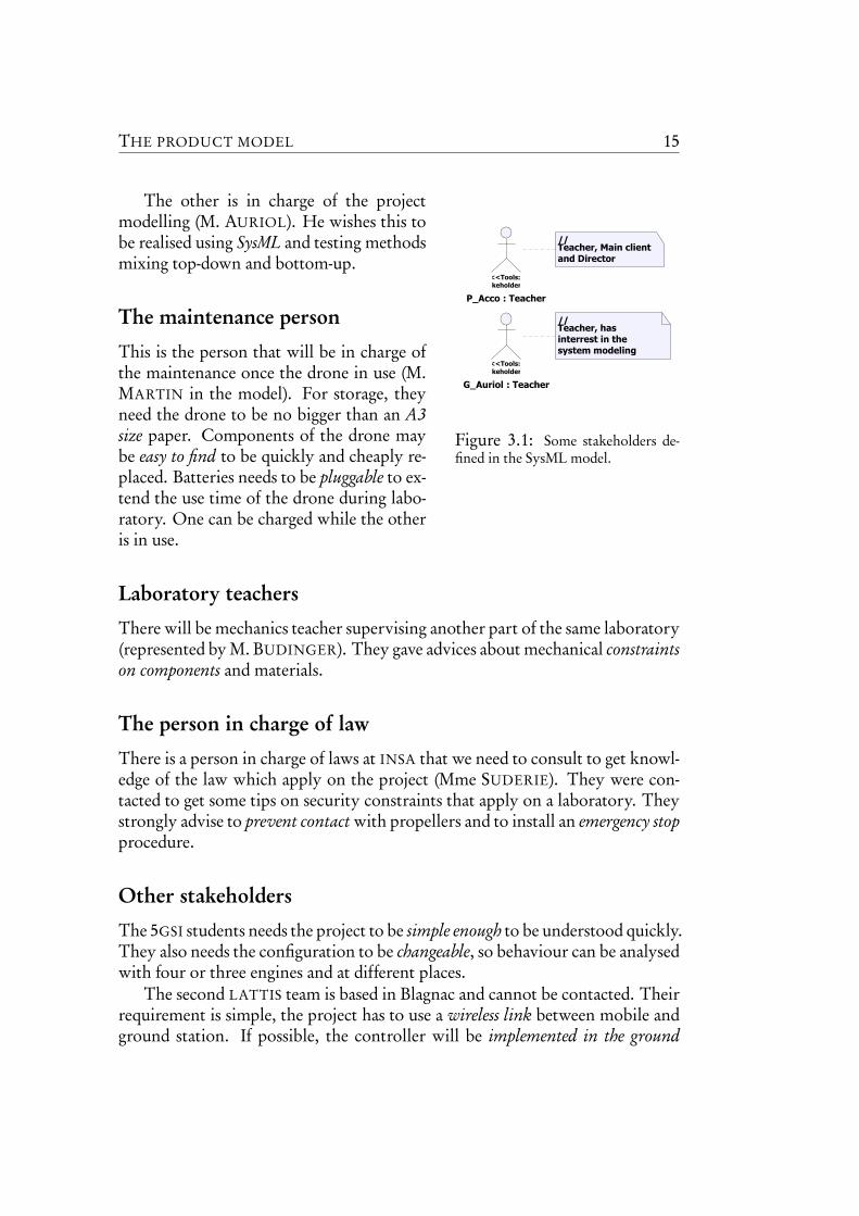
We have two training supervisors in this internship project. One is the personin charge of the automatic control part (M. ACCO on the model page A18). Heis the main supervisor and he wishes the project to conduct some tests on thesystem model to improve the product model. He would like a linearisation of themodel to be realised so to test observability and define possible output sensors.He recalls that the project is held by the academy and will be build by school.As a result, the mechanism have to be simple and cheap. He is also one of theteachers that will be in charge of the laboratory when the product is finished.
THE PRODUCT MODEL 15
package Stakeholders Use case diagram1 3/3
//Teacher, Main client
and Director
G_Auriol : Teacher
<<Tools::Stakeholder
//Teacher, has
interrest in the
system modeling
P_Acco : Teacher
<<Tools::Stakeholder
Figure 3.1: Some stakeholders de-fined in the SysML model.
The other is in charge of the projectmodelling (M. AURIOL). He wishes this tobe realised using SysML and testing methodsmixing top-down and bottom-up.
The maintenance person
This is the person that will be in charge ofthe maintenance once the drone in use (M.MARTIN in the model). For storage, theyneed the drone to be no bigger than an A3size paper. Components of the drone maybe easy to find to be quickly and cheaply re-placed. Batteries needs to be pluggable to ex-tend the use time of the drone during labo-ratory. One can be charged while the otheris in use.
Laboratory teachers
There will be mechanics teacher supervising another part of the same laboratory(represented by M. BUDINGER). They gave advices about mechanical constraintson components and materials.
The person in charge of law
There is a person in charge of laws at INSA that we need to consult to get knowl-edge of the law which apply on the project (Mme SUDERIE). They were con-tacted to get some tips on security constraints that apply on a laboratory. Theystrongly advise to prevent contact with propellers and to install an emergency stopprocedure.
Other stakeholders
The 5GSI students needs the project to be simple enough to be understood quickly.They also needs the configuration to be changeable, so behaviour can be analysedwith four or three engines and at different places.
The second LATTIS team is based in Blagnac and cannot be contacted. Theirrequirement is simple, the project has to use a wireless link between mobile andground station. If possible, the controller will be implemented in the ground
16 CONTROL OF A MINI UNMANNED AERIAL VEHICULE
station and the wireless link will be used to transmit inputs and outputs but notreference.
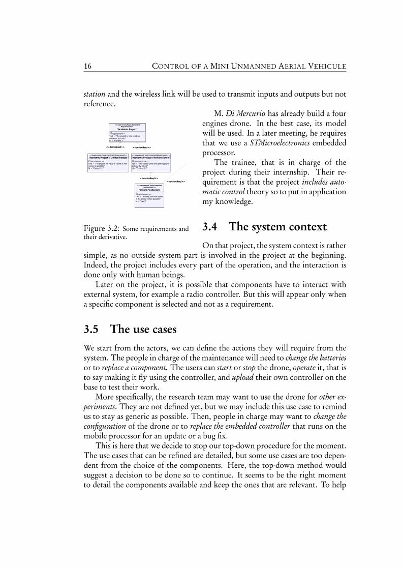
«»
<<requirement,Tools::UseabilityRequirement>>
'Simple Mechanism'
<<requirement>>Text = "Building the final object in the school will be possible"Id = "Use.2"
«»
<<requirement,Tools::ConstraintRequirement>>
'Academic Project'
<<requirement>>Text = "The project is held inside an academic structure"Id = "Context.2"
«»
<<requirement,Tools::ConstraintRequirement>>
'Academic Project'::'Limited Budget'
<<requirement>>Text = "The project will have to spend as few money as possible."Id = "Context.2.1"
«»
<<requirement,Tools::ConstraintRequirement>>
'Academic Project'::'Built by School'
<<requirement>>Text = "The objects (final and prototype) will be build by school"Id = "Context.2.2"
«»
requirement,Tools::ConstraintRequirement
SecundaryRequirements::'Low deformation'
<<requirement>>Id = "Mecha.1"Text = "The structure should have a low deformation"
«»
<<requirement,Tools::ConstraintRequirement>>
SecundaryRequirements::Resonance
<<requirement>>Id = "Mecha.2"Text = "The modes of the structure will be designed so there is no resonance"
«»
<<requirement,Tools::ConstraintRequirement>>
SecundaryRequirements::Vibration
<<requirement>>Id = "Mecha.3"Text = "The structure will minimise vibrations"
«»
<<requirement,Tools::ConstraintRequirement>>
SecundaryRequirements::'Hard stiffness'
<<requirement>>Id = "Mecha.1.1"Text = "The structure will be design so its stiffness is high"
<<deriveReqt>>
<<deriveReqt>>
<<deriveReqt>> <<deriveReqt>>
<<deriveReqt>><<deriveReqt>>
<<deriveReqt>>
<<block>>
Environment::MUAV::Structure
<<satisfy>>
Figure 3.2: Some requirements andtheir derivative.
M. Di Mercurio has already build a fourengines drone. In the best case, its modelwill be used. In a later meeting, he requiresthat we use a STMicroelectronics embeddedprocessor.
The trainee, that is in charge of theproject during their internship. Their re-quirement is that the project includes auto-matic control theory so to put in applicationmy knowledge.
3.4 The system contextOn that project, the system context is rather
simple, as no outside system part is involved in the project at the beginning.Indeed, the project includes every part of the operation, and the interaction isdone only with human beings.
Later on the project, it is possible that components have to interact withexternal system, for example a radio controller. But this will appear only whena specific component is selected and not as a requirement.
3.5 The use casesWe start from the actors, we can define the actions they will require from thesystem. The people in charge of the maintenance will need to change the batteriesor to replace a component. The users can start or stop the drone, operate it, that isto say making it fly using the controller, and upload their own controller on thebase to test their work.
More specifically, the research team may want to use the drone for other ex-periments. They are not defined yet, but we may include this use case to remindus to stay as generic as possible. Then, people in charge may want to change theconfiguration of the drone or to replace the embedded controller that runs on themobile processor for an update or a bug fix.
This is here that we decide to stop our top-down procedure for the moment.The use cases that can be refined are detailed, but some use cases are too depen-dent from the choice of the components. Here, the top-down method wouldsuggest a decision to be done so to continue. It seems to be the right momentto detail the components available and keep the ones that are relevant. To help
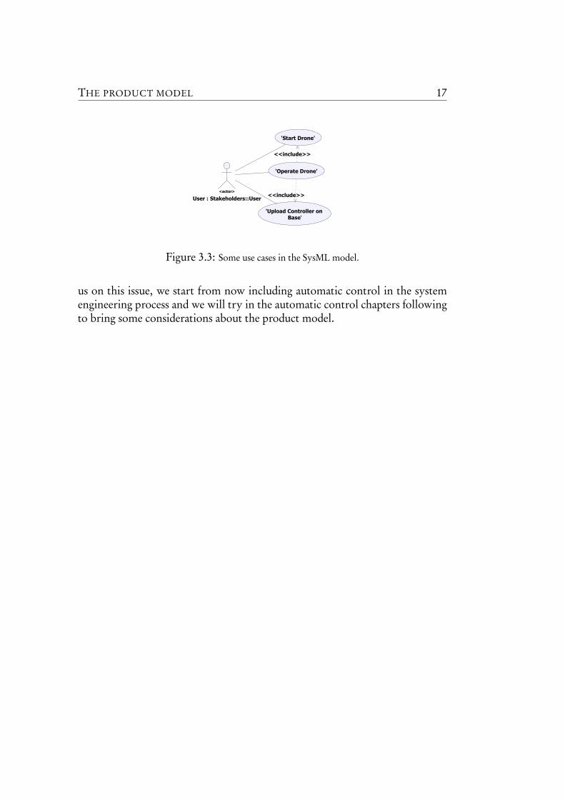
THE PRODUCT MODEL 17package UseCases Use case diagram1 3/3
User : Stakeholders::User
<<actor>>
'Start Drone'
'Operate Drone'
'Upload Controller on
Base'
<<include>>
<<include>>
Figure 3.3: Some use cases in the SysML model.
us on this issue, we start from now including automatic control in the systemengineering process and we will try in the automatic control chapters followingto bring some considerations about the product model.

18 CONTROL OF A MINI UNMANNED AERIAL VEHICULE
Chapter 4The non linear model
In the following chapters, we switch to automatic control of the MUAV itself,but we still have in mind the problematics stated by the product model.
On the automatic control part, a huge work has already been done. AnIntegrated Project was held by an INSA student, Aurélie SOULETIS during her5th year. In her report[7], Souletis realises the mechanical and physical model ofa four engines MUAV. It is strongly recommended to read her paper first if youare willing to work on the non linear model. However, the next sections willrecall the main results. Some extension will also be done as we now target othernumber of engines than four.
4.1 Mechanical bases used
The drone is considered as a unique solid, completely unbound from the earthexcept the gravity force that applies on it. We define two frames attached tothe centre of gravity of the drone. The first one is the inertia frame Ri , whose
orientation is bound to earth. At any moment, its unit vectors−→e i1 and
−→e i2 are
parallel to the ground, while−→e i3 is orthogonal and points toward the ground.
The basis is orthonormal. The second frame is the mobile frame Rm , whoseorientation is attached to the drone and constituted by the orthonormal vectors−→e m1 ,−→e m2 and
−→e m3 . When its attitude* is flat and yaw* is null, the two basis are
identical.To describe the mobile orientation, we use Euler’s angles φ, θ and ψ, three
consecutive rotations around e m3 , e m
2 and e m1 respectively. As a result, we can
20 CONTROL OF A MINI UNMANNED AERIAL VEHICULE
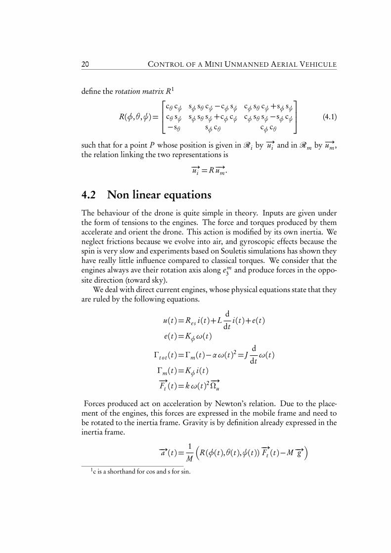
define the rotation matrix R1
R(φ,θ,ψ)=
cθ cψ sφ sθ cψ−cφ sψ cφ sθ cψ+sφ sψcθ sψ sφ sθ sψ+cφ cψ cφ sθ sψ−sφ cψ−sθ sφ cθ cφ cθ
(4.1)
such that for a point P whose position is given inRi by −→ui and inRm by −→um ,the relation linking the two representations is
−→ui =R−→um .
4.2 Non linear equationsThe behaviour of the drone is quite simple in theory. Inputs are given underthe form of tensions to the engines. The force and torques produced by themaccelerate and orient the drone. This action is modified by its own inertia. Weneglect frictions because we evolve into air, and gyroscopic effects because thespin is very slow and experiments based on Souletis simulations has shown theyhave really little influence compared to classical torques. We consider that theengines always ave their rotation axis along e m
3 and produce forces in the oppo-site direction (toward sky).
We deal with direct current engines, whose physical equations state that theyare ruled by the following equations.
u(t )=Re s i(t )+Ld
dti(t )+ e(t )
e(t )=Kφω(t )
Γt ot (t )=Γm(t )−αω(t )2= J
d
dtω(t )
Γm(t )=Kφ i(t )−→Ft (t )= kω(t )2
−→Ωu
Forces produced act on acceleration by Newton’s relation. Due to the place-ment of the engines, this forces are expressed in the mobile frame and need tobe rotated to the inertia frame. Gravity is by definition already expressed in theinertia frame.
−→a (t )=1
M
R(φ(t ),θ(t ),ψ(t ))−→Ft (t )−M−→g
1c is a shorthand for cos and s for sin.
THE NON LINEAR MODEL 21
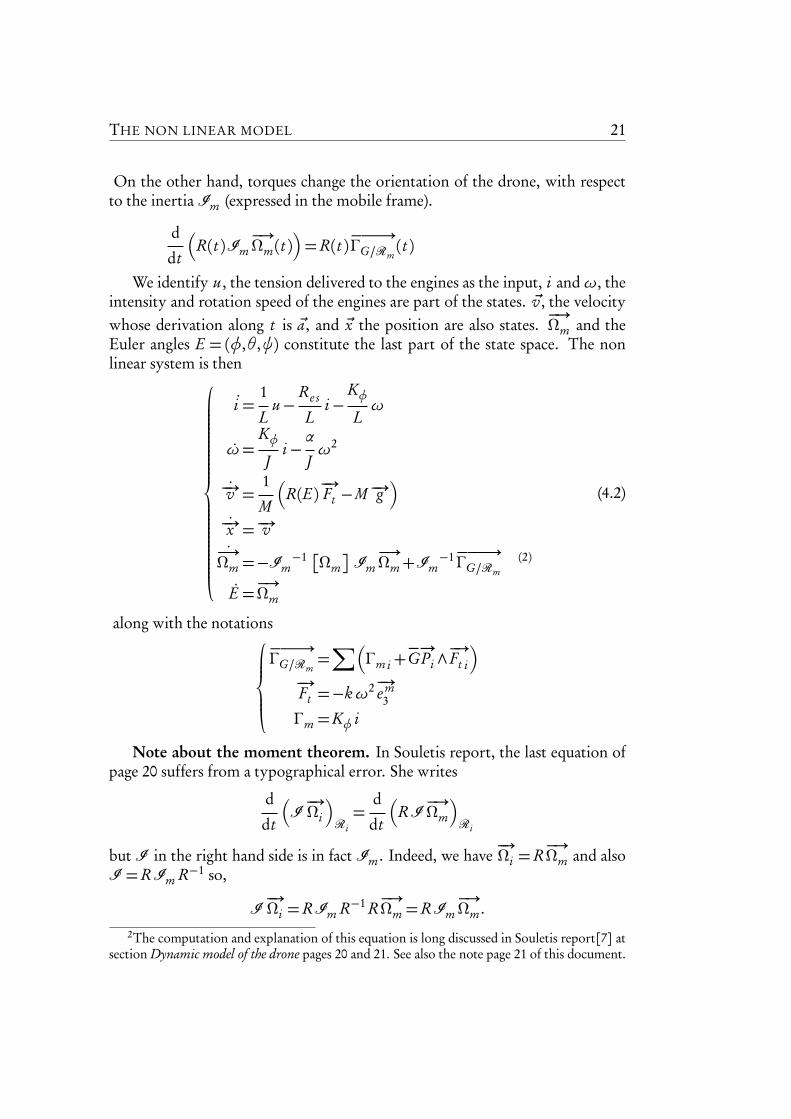
On the other hand, torques change the orientation of the drone, with respectto the inertia Im (expressed in the mobile frame).
d
dt
R(t )Im−→Ωm(t )
=R(t )−−−→ΓG/Rm
(t )
We identify u, the tension delivered to the engines as the input, i andω, theintensity and rotation speed of the engines are part of the states. ~v, the velocitywhose derivation along t is ~a, and ~x the position are also states.
−→Ωm and the
Euler angles E = (φ,θ,ψ) constitute the last part of the state space. The nonlinear system is then
i =1
Lu−
Re s
Li−
KφLω
ω=KφJ
i−α
Jω2
−→v =1
M
R(E)−→Ft −M−→g
−→x =−→v−→Ωm =−Im
−1 Ωm
Im−→Ωm+Im
−1−−−→ΓG/Rm
(2)
E =−→Ωm
(4.2)
along with the notations
−−−→ΓG/Rm
=∑
Γm i+−→GPi ∧
−→Ft i
−→Ft =−kω2−→e m
3
Γm =Kφ i
Note about the moment theorem. In Souletis report, the last equation ofpage 20 suffers from a typographical error. She writes
d
dt
I −→Ωi
Ri=
d
dt
RI −→Ωm
Ri
but I in the right hand side is in fact Im . Indeed, we have−→Ωi =R
−→Ωm and also
I =RIm R−1 so,
I −→Ωi =RIm R−1 R−→Ωm =RIm
−→Ωm .
2The computation and explanation of this equation is long discussed in Souletis report[7] atsection Dynamic model of the drone pages 20 and 21. See also the note page 21 of this document.
22 CONTROL OF A MINI UNMANNED AERIAL VEHICULE
4.3 Simulink® modelAurélie SOULETIS already provided a correct Simulink model of the MUAV. Butwe needed this model to be extensible to any number of engines. I also wantedto get rid of the m-blocks that are converted to mex files* and hard-compiled byMATLAB®. These blocks become unportable and need some manipulation toget them working again on another architecture. So I wanted to replace them bylevel-2 m-files*. The new Simulink model is presented in appendix A page A1.
Chapter 5Fixed point computation
From the non linear model, we can define the system fixed points, that is tosay the points in the state space where the MUAV can stay naturally indefinitely.They are also very interesting for the product model as a structure that do notpresent any fixed point will be harder to control, less stable, may be impossibleto control and will probably not meet the requirement of simplicity.
5.1 The engines
The engines constitute rather independent systems. Hence, we can study theirfixed points separately from the rest of the system. One engine is ruled by thefollowing equations
i =1
Lu−
Re s
Li−
KφLω (5.1)
ω=KφJ
i−α
Jω2 (5.2)
the state being (i ,ω). We want this state to be static, that is to say we want(i0,ω0)= (0,0). Equation (5.2) gives
i0=α
Kφω0
2 (5.3)
so (5.1) becomesRe s αω0
2+Kφω0−Kφ u0= 0
24 CONTROL OF A MINI UNMANNED AERIAL VEHICULE
which gives us the final relation between u andω,
ω0=−K2
φ±q
K4φ+4KφαRe s u0
2αR. (5.4)
This equation has to be repeated for each engine with their respective param-eters.
5.2 OrientationTo get a fixed point, we need the MUAV to be static regarding orientation. Wediscard for the moment the special case when the MUAV spins around its verticalaxis. So the angular velocity has to be null,
−−→Ωm0=
−→0 .
Hence, the equation extracted from the moment theorem become rather simple.
˙−−→Ωm0=−I
−1 Ωm0
I −−→Ωm0+I−1−−−−→ΓG/Rm 0
=I −1−−−−→ΓG/Rm 0(5.5)
Moreover, this angular velocity must not vary from its zero, so we also have
˙−−→Ωm0=
−→0 .
Now, equation (5.5) writes
−→0 =I −1−−−−→ΓG/Rm 0
⇐⇒ −→0 =−−−−→ΓG/Rm 0
⇐⇒ −→0 =
∑−−→Γm i 0+
−→GPi ∧
−→Ft i 0
. (5.6)
Concerning the projection of the vectors,−→Γm i is a vector along
−→e m3 while
−→GPi
applies according to−→e m1 and
−→e m2 only and
−→Ft i is along
−→e m3 . As a result,
−→GPi ∧
−→Ft i
is a vector according to−→e m1 and
−→e m2 only. We can project equation (5.6) on the
basis vectors,
e m1 : 0=
∑
GPi y Ft i 0
e m2 : 0=
∑
GPi x Ft i 0e m3 : 0=
∑
Γm i 0
(5.7)
FIXED POINT COMPUTATION 25
When engines are built so that for an upward force, they can spin, someclockwise and the others counterclockwise, then there will be negative torquesnorms and the equation in e m
3 can be fulfilled. Let di be either 1 or−1 accordingto the rotation direction (clockwise or counterclockwise) needed for the enginei to produce an upward force. the equations on e m
1 and e m2 and equation (5.3)
can also be merged. The relations are now
e m1 : 0=
∑
GPi yki Kφ iαi
ii 0
e m2 : 0=
∑
GPi xki Kφ iαi
ii 0
e m3 : 0=
∑
di Kφiii 0
(5.8)
but they can’t really be more developed if we cannot make assumptions on theMUAV architecture. These equations are fundamental to decide whether a givenarchitecture (number of engines and their placement on the structure) will be viableor not. We call them the realisability equations. We have here a good example ofwhat including automatic control in the system engineering process can bring.These equations must be considered as a requirement in the SysML model.
5.3 PositionIn practice, we don’t consider the need either for position or for velocity to benull to get a fixed point. A static position or a uniform motion at any point ofthe space is here considered to be a fixed point. As a result, we will only considerthe equation
−→v0 =1
M
R(φ0,θ0,ψ0)∑−→
Ft i 0−M−→g
=−→0
that we can project on the vectors of the inertia basis.
e i1 : 0= 1
M (cφ0sθ0 cψ0
+sφ0sψ0)∑
Ft i 0
e i2 : 0= 1
M (cφ0sθ0 sψ0
−sφ0cψ0)∑
Ft i 0
e i3 : 0= 1
M (cφ0cθ0 )
∑
Ft i 0− g(5.9)
The projection in e i3 tells that
∑
Ft i 0 must be non null for a solution toexist. Neither should be the product cφ0
cθ0 . Hence, there are restrictions onthe angles.
cφ0sθ0 cψ0
+sφ0sψ0= 0
cφ0sθ0 sψ0
−sφ0cψ0= 0
cφ0cθ0 6= 0
26 CONTROL OF A MINI UNMANNED AERIAL VEHICULE
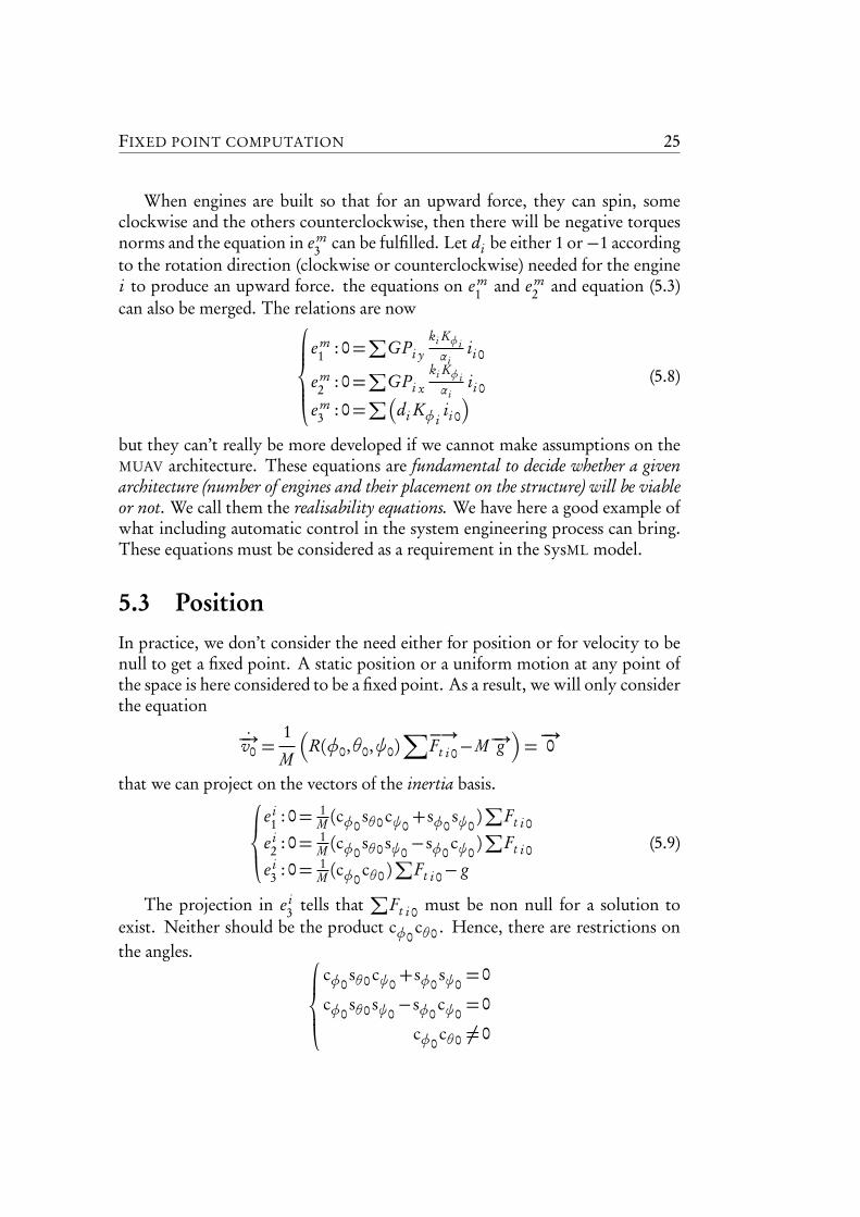
Figure 5.1: A non flat attitude pro-duces an horizontal acceleration.
It is clear that we need a perfectly flat trimto achieve a fixed point, but that the yawis a parameter that doesn’t play a role init. Indeed, it is at this only one conditionthat the projection of
−→Ft in the inertia basis
(provided that the vertical component can-cels the effect of gravity) does not produce anull vector in the horizontal plane that willincrease horizontal speed. Indeed, the solu-tion of this system (computed using a CAS*)is φ0= 0, θ0= 0 and ψ0 ∈ (−π;π]. If φ0 orθ0 are different from zero, forces don’t bal-
ance and Newton’s first law tells us that there is no uniform motion or state ofrest possible.
We end with that simple relation
∑
Ft i 0=M g . (5.10)
Remark that this result doesn’t exclude the uniform motion from the possiblefixed points. That also means that simply flattening the MUAV attitude will notbe sufficient to stop it (considering, of course, air friction too low to decreasespeed in a short enough time).
We can link that result to the engines thanks to the equation (5.3).
∑
i
ki Kφi
αiii 0=M g (5.11)
5.4 Application to the four engines MUAV
The structure of this MUAV includes four engines placed at the same distance rfrom the centre, each arm of the MUAV is separated from the others by a 90
angle. As a result,−→GPi are defined as
−−→GP1=
r00
,−−→GP2=
0−r0
,−−→GP3=
−r00
and−−→GP4=
0r0
.
Moreover, engines are identical, their characteristics are equals. Engines 1 and 2rotate in one direction (for example, clockwise), while engines 2 and 4 rotate in
FIXED POINT COMPUTATION 27
the other (counterclockwise). We can simplify equation (5.8)
e m1 : 0=
k Kφα (i10− i30)
e m2 : 0=
k Kφα (i40− i20)
e m3 : 0=Kφ(i10− i20+ i30− i40)
(5.12)
which gives the unique possible result, i10= i20= i30= i40= i0. Hence, equation(5.11) writes
4k Kφα
i0=M g
⇐⇒ i0=M g
4·α
k Kφ(5.13)
which, combined with (5.3) gives
ω0=
È
M g
4k. (5.14)
As a result, the input needed to produce such a fixed point is u10= u20= u30=u40= u0 such that
u0=Re s α
Kφ·
M g
4k+Kφ
È
M g
4k(5.15)
due to equation (5.1).
5.5 Note about holonomyA mobile always evolve in a defined space —a real solid space, not to be con-founded with state space— made of dimensions. For many, it is 2D, othersevolve inside a 3D space, and some along a unique dimension. It is provedthat for a space of dimension d , one can apply to a mobile d translations andd (d −1)/2 rotations. For example, a robot evolving on a plane has 2 transla-tions: surge* (forward and backward), sway* (step left or right); and 1 rotation:yaw*.
The degrees of manœuvrability are the number of movements that the ac-tuators altogether can produce on a system. Normally, each actuator providesone or more degree of manœuvrability, but if they are not chosen and placedintelligently enough, two actuators can finally do the same job and provide both
28 CONTROL OF A MINI UNMANNED AERIAL VEHICULE
the same of manœuvrability. When degrees of manœuvrability are fewer thandegrees of freedom, the system is said non-holonomic. It is holonomic when bothare equals, and can even be redundant if there is more degrees of manœuvrabilitythan degrees of freedom. This situation is sometimes a good point to achieve abetter control or precision on the movements.
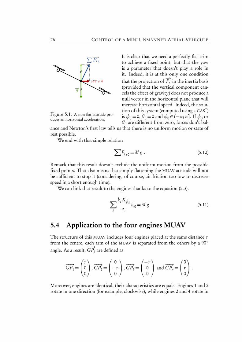
Figure 5.2: The three rotations al-lowed in 3D space. [14]
Our MUAV evolves in 3D space, so hasbasically 3 translations: surge, sway andheave* (up and down); and 3 rotations:pitch*, yaw and roll*. As these movementsare not limited by any junction (at leastwhen flying off the ground), the MUAV has6 degrees of freedom. In the four enginesconfigurations, we can apply four distinctinputs on the mobile and as the placementof engines are intelligent enough and eachactuator works in one dimension, we havefour degrees of manœuvrability. We can seethat we are already non-holonomic. First,we control heave and yaw. Then, we canchoose to control either pitch or surge and either roll or sway. The degrees offreedom that are not controlled are in that precise case reachable, meaning thatwe can make the MUAV be at a desired state at one moment but we can’t providea way to be sure it will keep this state longer. Indeed, if we want to keep indef-initely the MUAV at an exact position in space (including altitude) and a fixedyaw, it is then impossible to choose any value for pitch and roll. Only φ= 0and θ= 0 provide stability in position. On the other hand, it is possible to fixthe three Euler angles of the MUAV so it has the desired attitude and to fix thealtitude. But then, the MUAV will move in a 2D-plane parallel to the ground.
Now, it becomes evident that a three engines MUAV will unavoidably loosethe control of one (possibly more) degree of freedom. Sticking with the config-uration where engines are along e m
3 , we loose the control on the yaw.
5.6 Study of a 3 engines MUAV
We consider now a MUAV built with 3 engines of different characteristics, placedat different distances from the centre and with arms making an unknown anglewith their neighbours. It is clear, according to the e m
3 component of equation(5.8), that we will need one engine rotating the opposite direction of the twoothers, and its produced torque will need to cancel the two others. To achievethis, we can either make it spin faster, or dimension it so it produces more torque
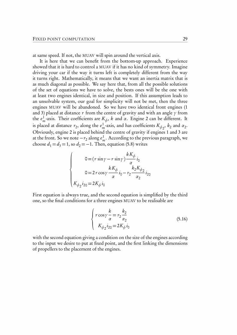
FIXED POINT COMPUTATION 29
at same speed. If not, the MUAV will spin around the vertical axis.It is here that we can benefit from the bottom-up approach. Experience
showed that it is hard to control a MUAV if it has no kind of symmetry. Imaginedriving your car if the way it turns left is completely different from the wayit turns right. Mathematically, it means that we want an inertia matrix that isas much diagonal as possible. We say here that, from all the possible solutionsof the set of equations we have to solve, the bests ones will be the one withat least two engines identical, in size and position. If this assumption leads toan unsolvable system, our goal for simplicity will not be met, then the threeengines MUAV will be abandoned. So we have two identical front engines (1and 3) placed at distance r from the centre of gravity and with an angle γ fromthe e1
m -axis. Their coefficients are Kφ, k and α. Engine 2 can be different. Itis placed at distance r2, along the e1
m -axis, and has coefficients Kφ2, k2 and α2.
Obviously, engine 2 is placed behind the centre of gravity if engines 1 and 3 areat the front. So we note−r2 along e1
m . According to the previous paragraph, wechoose d1= d3= 1, so d2=−1. Then, equation (5.8) writes
0=(r sinγ− r sinγ )k Kφα
i0
0= 2 r cosγk Kφα
i0− r2
k2 Kφ2
α2i20
Kφ2i20= 2Kφ i0
First equation is always true, and the second equation is simplified by the thirdone, so the final conditions for a three engines MUAV to be realisable are
r cosγk
α= r2
k2
α2
Kφ2i20= 2Kφ i0
(5.16)
with the second equation giving a condition on the size of the engines accordingto the input we desire to put at fixed point, and the first linking the dimensionsof propellers to the placement of the engines.

30 CONTROL OF A MINI UNMANNED AERIAL VEHICULE
Chapter 6Linearisation of system model
Once we have defined the fixed points of the system, we want to ensure theyare stable or that we can control them to be stable. We also need to know if itis possible through the chosen sensors to gather enough information from thesystem to achieve this control. To simplify this task, it is better to use a linearrepresentation of the system around the studied fixed point that directly use thenon linear equations.
The same approach is used as for the fixed point, the engines are studiedfirst and the results are propagated to the action the engines have on the droneposition and orientation.
6.1 About the linearisation processThe linearisation process is a mathematical operation that approximates a nonlinear function around one of its points, by a line. This approximation is givenby the Taylor expansion of the function around the chosen point. For example,the Taylor expansion of a function f of X and U is
f (X ,U )= f (X0,U0)+∂ f (X ,U )
∂ X
X0U=U0
∂ X
+∂ f (X ,U )
∂ U
X=X0U0
∂ U +∂ 2 f
∂ 2X. . .
In system control, this approximation is done around a fixed point so thatf (X0,U0) = 0. Hence, the new model written is a model that represents thevariations of output and state according to little variations of the input around
32 CONTROL OF A MINI UNMANNED AERIAL VEHICULE
the fixed point. As variations are little, higher order terms are small enough tobe negligible. Finally, and only around a fixed point and for small variations, thefunction can be approximated by
f (X ,U )=∂ f (X ,U )
∂ X
X0U=U0
∂ X +∂ f (X ,U )
∂ U
X=X0U0
∂ U (6.1)
The linearisation is used here to study observability, stability and compute astate feedback control for the system. The principle used here is the study of thebest case. That is, we state that if the computation do not work for the simplifiedlinearised model, then it will not work either on the non linear system.
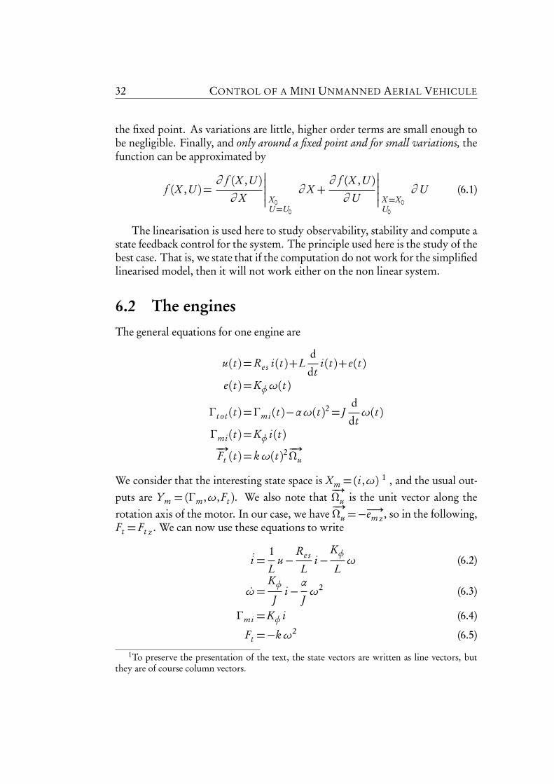
6.2 The enginesThe general equations for one engine are
u(t )=Re s i(t )+Ld
dti(t )+ e(t )
e(t )=Kφω(t )
Γt ot (t )=Γmi (t )−αω(t )2= J
d
dtω(t )
Γmi (t )=Kφ i(t )−→Ft (t )= kω(t )2
−→Ωu
We consider that the interesting state space is Xm = (i ,ω) 1 , and the usual out-puts are Ym = (Γm ,ω,Ft ). We also note that
−→Ωu is the unit vector along the
rotation axis of the motor. In our case, we have−→Ωu =−
−→em z , so in the following,Ft = Ft z . We can now use these equations to write
i =1
Lu−
Re s
Li−
KφLω (6.2)
ω=KφJ
i−α
Jω2 (6.3)
Γmi =Kφ i (6.4)
Ft =−kω2 (6.5)
1To preserve the presentation of the text, the state vectors are written as line vectors, butthey are of course column vectors.
LINEARISATION OF SYSTEM MODEL 33
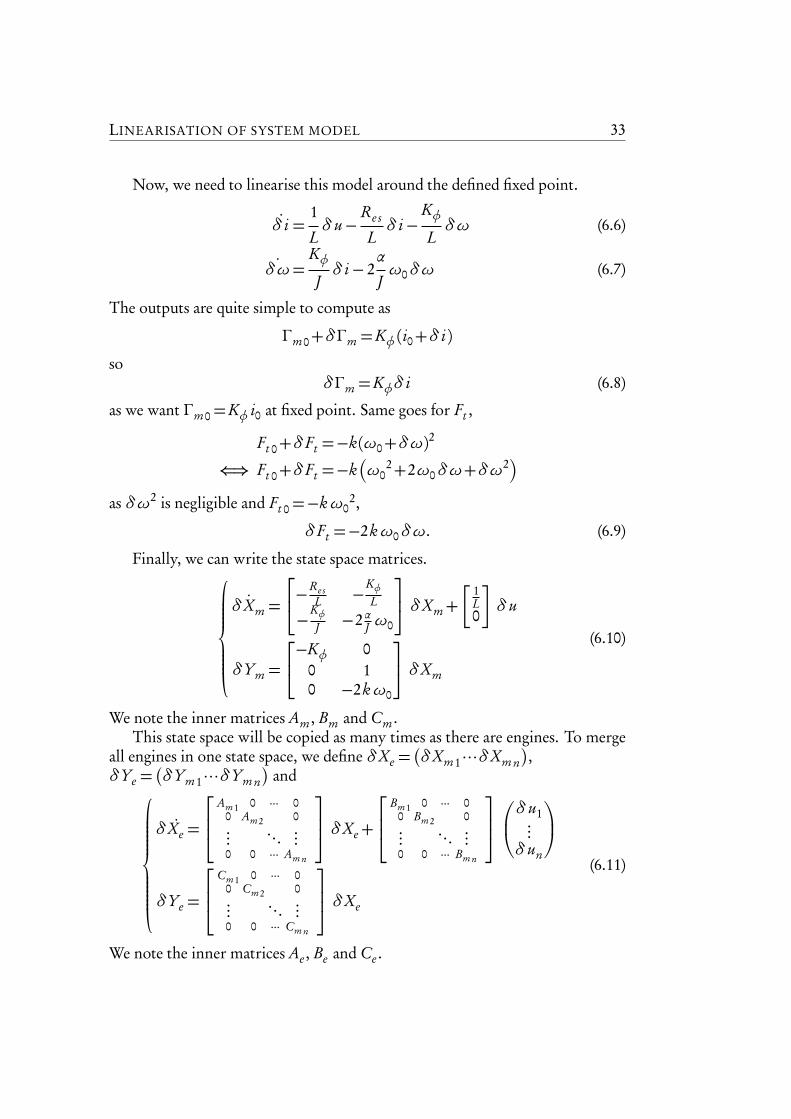
Now, we need to linearise this model around the defined fixed point.
δ i =1
Lδu−
Re s
Lδ i−
KφLδω (6.6)
δω=KφJδ i− 2
α
Jω0δω (6.7)
The outputs are quite simple to compute as
Γm0+δΓm =Kφ (i0+δ i)
soδΓm =Kφδ i (6.8)
as we want Γm0=Kφ i0 at fixed point. Same goes for Ft ,
Ft 0+δFt =−k(ω0+δω)2
⇐⇒ Ft 0+δFt =−k
ω02+2ω0δω+δω
2
as δω2 is negligible and Ft 0=−kω02,
δFt =−2kω0δω. (6.9)
Finally, we can write the state space matrices.
˙δXm =
−Re sL −
KφL
−KφJ −2αJ ω0
δXm+
1L0
δu
δYm =
−Kφ 00 10 −2kω0
δXm
(6.10)
We note the inner matrices Am , Bm and Cm .This state space will be copied as many times as there are engines. To merge
all engines in one state space, we define δXe =
δXm1 · · ·δXm n
,δYe =
δYm1 · · ·δYm n
and
δXe =
Am1 0 ··· 00 Am2 0... ... ...0 0 ··· Am n
δXe+
Bm1 0 ··· 00 Bm2 0... ... ...0 0 ··· Bm n
δu1...
δun
δYe =
Cm1 0 ··· 00 Cm2 0... ... ...0 0 ··· Cm n
δXe
(6.11)
We note the inner matrices Ae , Be and Ce .
34 CONTROL OF A MINI UNMANNED AERIAL VEHICULE
6.3 Acceleration, velocity, positionFrom the engine state space, we note two important results. For one engine,we have a resultant force that varies around the fixed point as described by theequation (6.9). As the force generated by all the engines is the sum of resultantforces from each, it goes the same for the variations and we can write in a linearform
δFt =
0 −2kω01 · · · 0 −2kω0n
δXe .
We note this matrix C lFt
.
Newton’s equation,∑−→
F =M−→a , leads us to
−→a =1
M
−→Ft (Ri )
−M−→g
,
−→a being expressed in the inertia frame. As−→Ft is currently expressed in the
mobile frame, we have to apply to it the rotation matrix R. This rotation matrixdepends on the Euler angles that are part of the state space and change accordingto time during the process operation. We note E = (φ, θ,ψ) the Euler anglesand expand our current state vector Xa =
Xe , E
. Now we have
−→a (Xa)=1
M
R(E)−→Ft (Rm)
(Xe )−M−→g
.
As the force is only according to−→em3, only the last column of the rotation matrixis relevant. So the previous equation can be rewritten
−→a (Xa)=1
M
R(E)(:,3) Ft (Xe )−M
00g
.
R(E)(:,3) representing the third column of R(E). This vector can be consideredas a simple function. So we can write that this acceleration varies around its fixedpoint according to
δ−→a (Xa)=1
M·R(E0)(:,3) ·δFt +
1
M·Ft 0 ·
δR(E)(:,3)δE
E=E0
δE (6.12)
so we will need the rotation matrix and its first derivative according to E .The rotation matrix writes2
R(E)=
cθ cψ sφ sθ cψ−cφ sψ cφ sθ cψ+sφ sψcθ sψ sφ sθ sψ+cφ cψ cφ sθ sψ−sφ cψ−sθ sφ cθ cφ cθ
. (6.13)
2c is a shorthand for cos and s for sin.
LINEARISATION OF SYSTEM MODEL 35
Let us now compute the Jacobian of the function R(E)(:,3),
δR(E)(:,3)δE
=
−sφ sθ cψ+cφ sψ cφ cθ cψ −cφ sθ sψ+sφ cψ−sφ sθ sψ−cφ cψ cφ cθ sψ cφ sθ cψ+sφ sψ
−sφ cθ −cφ sθ 0
(6.14)
We note
AE/a =1
M·Ft 0 ·
δR(E)(:,3)δE
E=E0
the matrix representing the action of orientation variations on the force appliedto the drone. We can write
δ−→a = 1/M R(E0)(:,3)ClFt
︸ ︷︷ ︸
3×dim(δXe )
δXe+AE/a︸︷︷︸
3×3
δE . (6.15)
Now, we can add the velocity and position inside the state space (each hasthree coordinates expressed in the inertia frame) but in order to keep the statespace clean and readable, we split the Euler angles apart at the moment. Wedefine Xp =
Xe (vx vy vz) (x y z)
and Yp =
Ye (x y z)
. The state space canbe combined3
˙δXp =
Ae 0 01/M R(E0)(:,3)C
lFt
0 00 I3 0
δXp+
Be00
δU +
0AE/a
0
δE
δYp =
Ce 0 · · · 00 · · · 0 I3
δXp
with the inner matrices noted Ap , Bp and Cp for the next part. For simplicityof notation, we also state
C lg =R(E0)(:,3)C
lFt
.
6.4 OrientationThe orientation of the drone is influenced by the torques the engines apply to itand the moment theorem. The related equations are 4
−→Ωm =−Im
−1 Ωm
Im−→Ωm+Im
−1−−−→ΓG/Rm(6.16)
−−−→ΓG/Rm
=∑
Γmi+−→GPi ∧
−→Ft i
(6.17)
3In is the n by n identity matrix4Im is the inertia matrix written in the mobile base.
36 CONTROL OF A MINI UNMANNED AERIAL VEHICULE
It is quite straight forward to deduce that
δ−−−→ΓG/Rm
=∑
δΓmi+−→GPi ∧δ
−→Ft i
.
The equation of−→Ωm may seem a little bit trickier to linearise but in fact the
two terms of the sum depend on different state variables, so there is no crossderivation. We remind that inertia matrix is here independent from time andacts as a scalar. Only
Ωm
shall be linearised.We want to apply the change of variable
−→Ωm =
−−→Ωm0+δ
−→Ωm
that is
ωxωyωz
=
ωx 0ωy 0ωz 0
+
δωxδωyδωz
.
As a result,
Ωm
=
0 −ωz ωyωz 0 −ωx−ωy ωx 0
=
0 −ωz 0 ωy 0ωz 0 0 −ωx 0−ωy 0
ωx 0 0
+
0 −δωz δωyδωz 0 −δωx−δωy δωx 0
so
Ωm
=
Ωm0
+
δΩm
.
The equations (6.16) and (6.17) can be rearranged to be linearised
˙︷ ︷−−→Ωm0+δ
−→Ωm
=
Im−1 Ωm0
+
δΩm
Im
−−→Ωm0+δ
−→Ωm
+−−−−→ΓG/Rm 0
+δ−−−→ΓG/Rm
=
Im−1 Ωm0
Im+Im−1δΩm
Im
−−→Ωm0+δ
−→Ωm
+ . . .
=Im−1 Ωm0
Im−−→Ωm0+
−−−−→ΓG/Rm 0
︸ ︷︷ ︸
=˙−−→Ωm0=
−→0
+Im−1 Ωm0
Imδ−→Ωm
+Im−1δΩm
Im−−→Ωm0+Im
−1δΩm
Imδ−→Ωm
︸ ︷︷ ︸
negligible
+δ−−−→ΓG/Rm
LINEARISATION OF SYSTEM MODEL 37
and finally
˙δ−→Ωm =Im
−1 Ωm0
Imδ−→Ωm+Im
−1δΩm
Im−−→Ωm0
︸ ︷︷ ︸
+δ−−−→ΓG/Rm
(6.18)
Here, we come to a problem, because
δΩm
contains part of the state
space. We need to factor the complete equation Im−1δΩm
Im−−→Ωm0 to ex-
tract the components of δΩm .As we want to keep the equation general enough to allow any number of
motors, we will not make any assumption on the inertia matrix. We note
Im =
A −F −E−F B −D−E −D C
.
Im−1δΩm
Im−−→Ωm0=
1
C F 2+2D E F +B E2+AD2−AB C·V (δ−→Ωm)
38 CONTROL OF A MINI UNMANNED AERIAL VEHICULE
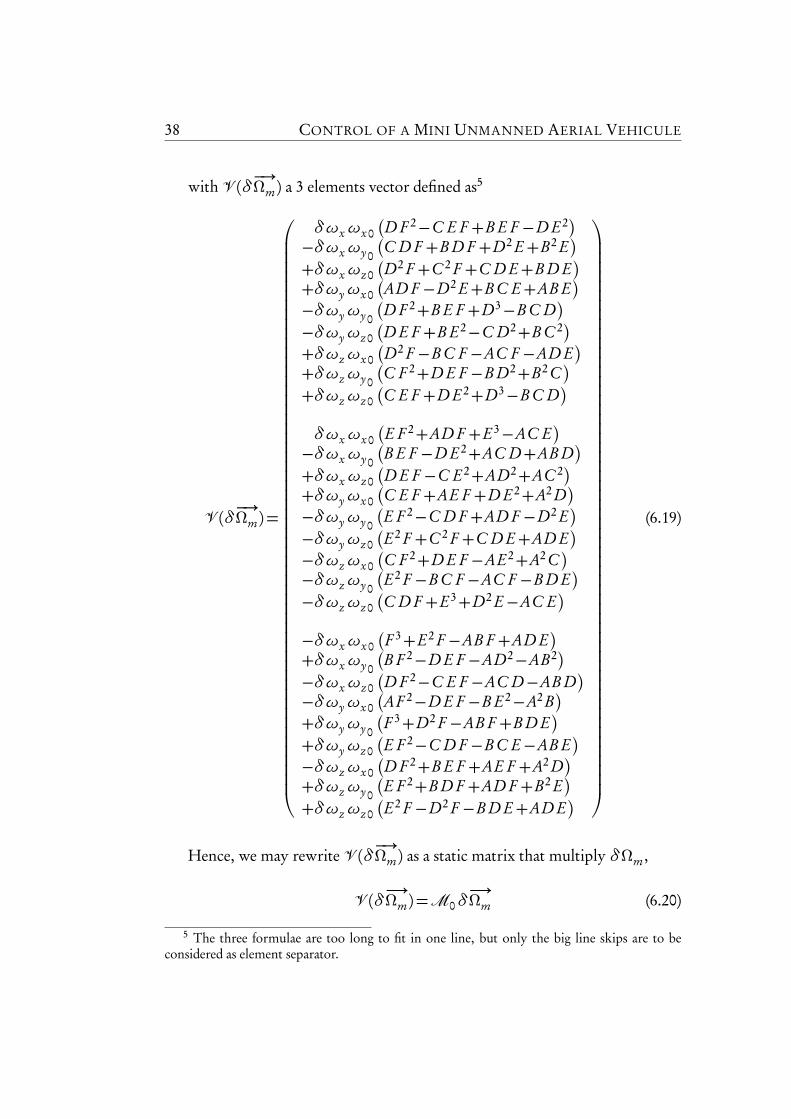
with V (δ−→Ωm) a 3 elements vector defined as5
V (δ−→Ωm)=
δωxωx 0
D F 2−C E F +B E F −D E2
−δωxωy 0
C D F +B D F +D2 E+B2 E
+δωxωz 0
D2 F +C 2 F +C D E+B D E
+δωyωx 0
AD F −D2 E+B C E+AB E
−δωyωy 0
D F 2+B E F +D3−B C D
−δωyωz 0
D E F +B E2−C D2+B C 2
+δωzωx 0
D2 F −B C F −AC F −AD E
+δωzωy 0
C F 2+D E F −B D2+B2 C
+δωzωz 0
C E F +D E2+D3−B C D
δωxωx 0
E F 2+AD F +E3−AC E
−δωxωy 0
B E F −D E2+AC D+AB D
+δωxωz 0
D E F −C E2+AD2+AC 2
+δωyωx 0
C E F +AE F +D E2+A2 D
−δωyωy 0
E F 2−C D F +AD F −D2 E
−δωyωz 0
E2 F +C 2 F +C D E+AD E
−δωzωx 0
C F 2+D E F −AE2+A2 C
−δωzωy 0
E2 F −B C F −AC F −B D E
−δωzωz 0
C D F +E3+D2 E−AC E
−δωxωx 0
F 3+E2 F −AB F +AD E
+δωxωy 0
B F 2−D E F −AD2−AB2
−δωxωz 0
D F 2−C E F −AC D−AB D
−δωyωx 0
AF 2−D E F −B E2−A2 B
+δωyωy 0
F 3+D2 F −AB F +B D E
+δωyωz 0
E F 2−C D F −B C E−AB E
−δωzωx 0
D F 2+B E F +AE F +A2 D
+δωzωy 0
E F 2+B D F +AD F +B2 E
+δωzωz 0
E2 F −D2 F −B D E+AD E
(6.19)
Hence, we may rewrite V (δ−→Ωm) as a static matrix that multiply δΩm ,
V (δ−→Ωm)=M0δ−→Ωm (6.20)
5 The three formulae are too long to fit in one line, but only the big line skips are to beconsidered as element separator.
LINEARISATION OF SYSTEM MODEL 39
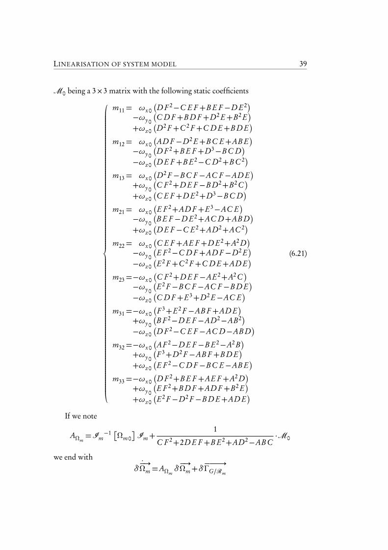
M0 being a 3×3 matrix with the following static coefficients
m11= ωx 0
D F 2−C E F +B E F −D E2
−ωy 0
C D F +B D F +D2 E+B2 E
+ωz 0
D2 F +C 2 F +C D E+B D E
m12= ωx 0
AD F −D2 E+B C E+AB E
−ωy 0
D F 2+B E F +D3−B C D
−ωz 0
D E F +B E2−C D2+B C 2
m13= ωx 0
D2 F −B C F −AC F −AD E
+ωy 0
C F 2+D E F −B D2+B2 C
+ωz 0
C E F +D E2+D3−B C D
m21= ωx 0
E F 2+AD F +E3−AC E
−ωy 0
B E F −D E2+AC D+AB D
+ωz 0
D E F −C E2+AD2+AC 2
m22= ωx 0
C E F +AE F +D E2+A2 D
−ωy 0
E F 2−C D F +AD F −D2 E
−ωz 0
E2 F +C 2 F +C D E+AD E
m23=−ωx 0
C F 2+D E F −AE2+A2 C
−ωy 0
E2 F −B C F −AC F −B D E
−ωz 0
C D F +E3+D2 E−AC E
m31=−ωx 0
F 3+E2 F −AB F +AD E
+ωy 0
B F 2−D E F −AD2−AB2
−ωz 0
D F 2−C E F −AC D−AB D
m32=−ωx 0
AF 2−D E F −B E2−A2 B
+ωy 0
F 3+D2 F −AB F +B D E
+ωz 0
E F 2−C D F −B C E−AB E
m33=−ωx 0
D F 2+B E F +AE F +A2 D
+ωy 0
E F 2+B D F +AD F +B2 E
+ωz 0
E2 F −D2 F −B D E+AD E
(6.21)
If we note
AΩm=Im
−1 Ωm0
Im+1
C F 2+2D E F +B E2+AD2−AB C·M0
we end with˙
δ−→Ωm =AΩm
δ−→Ωm+δ
−−−→ΓG/Rm
40 CONTROL OF A MINI UNMANNED AERIAL VEHICULE
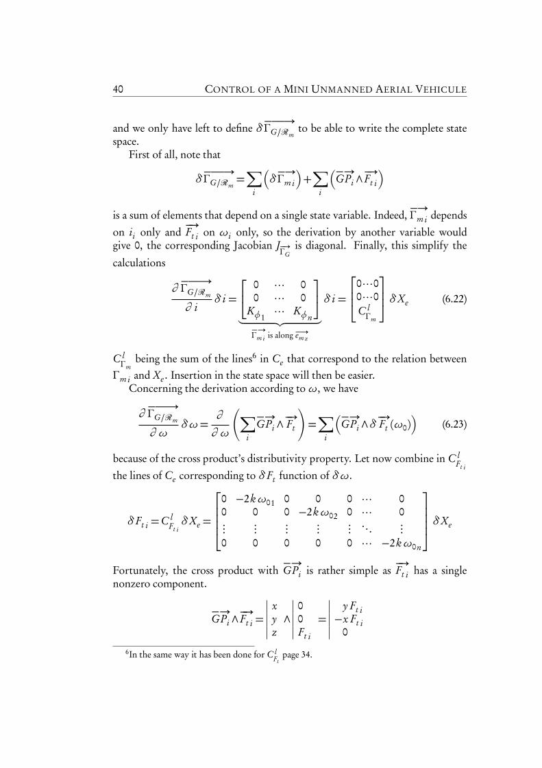
and we only have left to define δ−−−→ΓG/Rm
to be able to write the complete statespace.
First of all, note that
δ−−−→ΓG/Rm
=∑
i
δ−→Γm i
+∑
i
−→GPi ∧
−→Ft i
is a sum of elements that depend on a single state variable. Indeed,−→Γm i depends
on ii only and−→Ft i on ωi only, so the derivation by another variable would
give 0, the corresponding Jacobian J−→ΓG
is diagonal. Finally, this simplify the
calculations
∂−−−→ΓG/Rm
∂ iδ i =
0 · · · 00 · · · 0
Kφ1· · · Kφn
︸ ︷︷ ︸
−→Γm i is along −→em z
δ i =
0 · · ·00 · · ·0C lΓm
δXe (6.22)
C lΓm
being the sum of the lines6 in Ce that correspond to the relation betweenΓm i and Xe . Insertion in the state space will then be easier.
Concerning the derivation according toω, we have
∂−−−→ΓG/Rm
∂ ωδω=
∂
∂ ω
∑
i
−→GPi ∧
−→Ft
!
=∑
i
−→GPi ∧δ
−→Ft (ω0)
(6.23)
because of the cross product’s distributivity property. Let now combine in C lFt i
the lines of Ce corresponding to δFt function of δω.
δFt i =C lFt iδXe =
0 −2kω01 0 0 0 · · · 00 0 0 −2kω02 0 · · · 0...
......
...... . . . ...
0 0 0 0 0 · · · −2kω0n
δXe
Fortunately, the cross product with−→GPi is rather simple as
−→Ft i has a single
nonzero component.
−→GPi ∧
−→Ft i =
xyz∧
00Ft i
=y Ft i−x Ft i
0
6In the same way it has been done for C lFt
page 34.
LINEARISATION OF SYSTEM MODEL 41
Due to the form of C lFt i
, we can emulate this cross product by the multiplicationmatrix
h−→GPi
i
=
y1 y2 · · · yi−x1 −x2 · · · −xi
0 0 · · · 0
operation that is allowed thanks to the zeros filling the lines preventing unde-sired multiplications of
−→GPi with Ft j when i 6= j . Finally,
∑
i
−→GPi ∧δ
−→Ft (ω0)=
h−→GPi
i
C lFt i=C l
FG
that we insert into (6.23) to get
∂−−−→ΓG/Rm
∂ ωδω=C l
FGδXe . (6.24)
We also note from (6.22) and (6.24)
Aoe =Im−1
0 · · ·00 · · ·0C lΓm
+C lFG
and we get the final elements that can be inserted into the state space˙
δ−→Ωm =AΩm
δ−→Ωm+Aoe δXe (6.25)
Last but not least δ E =δ−→Ωm , that is to say
δ E = I3δ−→Ωm . (6.26)
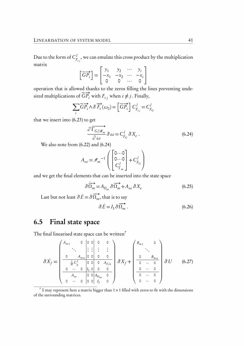
6.5 Final state space
The final linearised state space can be written7
δX f =
Am1 0 0 0 0 0... ...
......
...0 Am n 0 0 0 0
1M C l
g 0 0 0 AE/a
0 ··· 0 I3 0 0 0
Aoe 0 0 AΩm0
0 ··· 0 0 0 I3 0
δX f +
Bm1 0...
0 Bm n
0 ··· 0
0 ··· 0
0 ··· 0
0 ··· 0
δU (6.27)
7 0 may represent here a matrix bigger than 1×1 filled with zeros to fit with the dimensionsof the surrounding matrices.
42 CONTROL OF A MINI UNMANNED AERIAL VEHICULE
with δX f = (δXe ,δ−→Ωm ,δE). There is no output specified here because it will
strongly depend on the sensors placed to get them from the system. This will bedetermined later during the observability study.
Chapter 7Validation and model feedback
Once fixed point computed and linearisation established, we still have to testour equations and validate the results. To do so, we decided to simulate theequations using MATLAB. Component parameters are filled with the valuesgiven by Souletis’ report. It concerns a four engines drone equivalent to the onedescribed in section 5.4.
Then, we will be able to do some feedback on the SysML model to fill itwith what we found and possibly change and improve decisions we already madebefore.
7.1 Validation of the linear model
To validate the linear model, we can compare the outputs of both linear andnon linear models for little variation around the determined fixed point. ButSimulink allows us a more powerful comparison. Using the block Time BasedLinearisation (shown on page A2), we can ask Simulink to linearise the systemaround a given point on the simulation. Here, the given outputs and initial statesare set such that at time T = 1, the system is around fixed point.
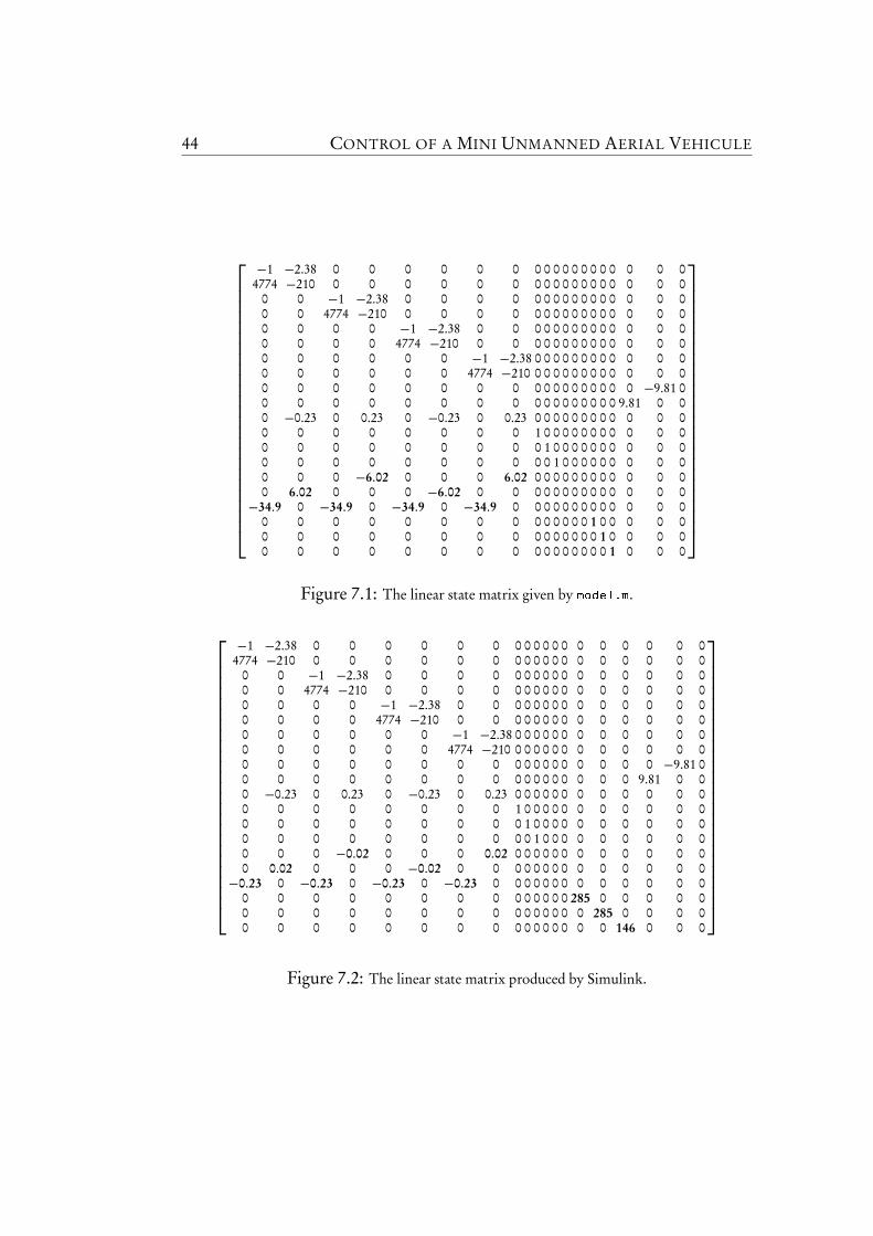
Then, we can compare the produced state matrix with the one obtained bythe linearised model in model.m (printed on page A9). Simulink doesn’t sortstates correctly so the matrices are mixed up and hard to compare but after com-pleting this jigsaw puzzle, it appears that matrices are almost the same exceptfor six values. They are highlighted on figures 7.1 and 7.2, and are indeed dueto the place Im
−1 is considered. In the linearisation done by model.m, the stateis really Ωm but in Simulink in fact, the state is ImΩm . To reduce operations,the state is multiplied by Im
−1 only after the integration as shown on page A2.
44 CONTROL OF A MINI UNMANNED AERIAL VEHICULE
−1 −2.38 0 0 0 0 0 0 0 0 0 0 0 0 0 0 0 0 0 04774 −210 0 0 0 0 0 0 0 0 0 0 0 0 0 0 0 0 0 0
0 0 −1 −2.38 0 0 0 0 0 0 0 0 0 0 0 0 0 0 0 00 0 4774 −210 0 0 0 0 0 0 0 0 0 0 0 0 0 0 0 00 0 0 0 −1 −2.38 0 0 0 0 0 0 0 0 0 0 0 0 0 00 0 0 0 4774 −210 0 0 0 0 0 0 0 0 0 0 0 0 0 00 0 0 0 0 0 −1 −2.38 0 0 0 0 0 0 0 0 0 0 0 00 0 0 0 0 0 4774 −210 0 0 0 0 0 0 0 0 0 0 0 00 0 0 0 0 0 0 0 0 0 0 0 0 0 0 0 0 0 −9.81 00 0 0 0 0 0 0 0 0 0 0 0 0 0 0 0 0 9.81 0 00 −0.23 0 0.23 0 −0.23 0 0.23 0 0 0 0 0 0 0 0 0 0 0 00 0 0 0 0 0 0 0 1 0 0 0 0 0 0 0 0 0 0 00 0 0 0 0 0 0 0 0 1 0 0 0 0 0 0 0 0 0 00 0 0 0 0 0 0 0 0 0 1 0 0 0 0 0 0 0 0 00 0 0 −6.02 0 0 0 6.02 0 0 0 0 0 0 0 0 0 0 0 00 6.02 0 0 0 −6.02 0 0 0 0 0 0 0 0 0 0 0 0 0 0
−34.9 0 −34.9 0 −34.9 0 −34.9 0 0 0 0 0 0 0 0 0 0 0 0 00 0 0 0 0 0 0 0 0 0 0 0 0 0 1 0 0 0 0 00 0 0 0 0 0 0 0 0 0 0 0 0 0 0 1 0 0 0 00 0 0 0 0 0 0 0 0 0 0 0 0 0 0 0 1 0 0 0
Figure 7.1: The linear state matrix given by model.m.
−1 −2.38 0 0 0 0 0 0 0 0 0 0 0 0 0 0 0 0 0 04774 −210 0 0 0 0 0 0 0 0 0 0 0 0 0 0 0 0 0 0
0 0 −1 −2.38 0 0 0 0 0 0 0 0 0 0 0 0 0 0 0 00 0 4774 −210 0 0 0 0 0 0 0 0 0 0 0 0 0 0 0 00 0 0 0 −1 −2.38 0 0 0 0 0 0 0 0 0 0 0 0 0 00 0 0 0 4774 −210 0 0 0 0 0 0 0 0 0 0 0 0 0 00 0 0 0 0 0 −1 −2.38 0 0 0 0 0 0 0 0 0 0 0 00 0 0 0 0 0 4774 −210 0 0 0 0 0 0 0 0 0 0 0 00 0 0 0 0 0 0 0 0 0 0 0 0 0 0 0 0 0 −9.81 00 0 0 0 0 0 0 0 0 0 0 0 0 0 0 0 0 9.81 0 00 −0.23 0 0.23 0 −0.23 0 0.23 0 0 0 0 0 0 0 0 0 0 0 00 0 0 0 0 0 0 0 1 0 0 0 0 0 0 0 0 0 0 00 0 0 0 0 0 0 0 0 1 0 0 0 0 0 0 0 0 0 00 0 0 0 0 0 0 0 0 0 1 0 0 0 0 0 0 0 0 00 0 0 −0.02 0 0 0 0.02 0 0 0 0 0 0 0 0 0 0 0 00 0.02 0 0 0 −0.02 0 0 0 0 0 0 0 0 0 0 0 0 0 0
−0.23 0 −0.23 0 −0.23 0 −0.23 0 0 0 0 0 0 0 0 0 0 0 0 00 0 0 0 0 0 0 0 0 0 0 0 0 0 285 0 0 0 0 00 0 0 0 0 0 0 0 0 0 0 0 0 0 0 285 0 0 0 00 0 0 0 0 0 0 0 0 0 0 0 0 0 0 0 146 0 0 0
Figure 7.2: The linear state matrix produced by Simulink.
VALIDATION AND MODEL FEEDBACK 45
Remarking that
285.7143×0.0211= 6.0286×1 and146.3415×0.2387= 34.9317×1,
we can say that the linearisations are similar, only one state intentionally differs.Hence, our linearisation is valid.
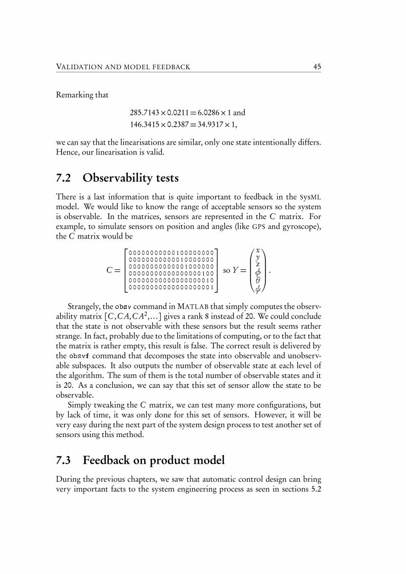
7.2 Observability testsThere is a last information that is quite important to feedback in the SysMLmodel. We would like to know the range of acceptable sensors so the systemis observable. In the matrices, sensors are represented in the C matrix. Forexample, to simulate sensors on position and angles (like GPS and gyroscope),the C matrix would be
C =
0 0 0 0 0 0 0 0 0 0 0 1 0 0 0 0 0 0 0 00 0 0 0 0 0 0 0 0 0 0 0 1 0 0 0 0 0 0 00 0 0 0 0 0 0 0 0 0 0 0 0 1 0 0 0 0 0 00 0 0 0 0 0 0 0 0 0 0 0 0 0 0 0 0 1 0 00 0 0 0 0 0 0 0 0 0 0 0 0 0 0 0 0 0 1 00 0 0 0 0 0 0 0 0 0 0 0 0 0 0 0 0 0 0 1
so Y =
xyzφθψ
.
Strangely, the obsv command in MATLAB that simply computes the observ-ability matrix [C ,C A,C A2, . . .] gives a rank 8 instead of 20. We could concludethat the state is not observable with these sensors but the result seems ratherstrange. In fact, probably due to the limitations of computing, or to the fact thatthe matrix is rather empty, this result is false. The correct result is delivered bythe obsvf command that decomposes the state into observable and unobserv-able subspaces. It also outputs the number of observable state at each level ofthe algorithm. The sum of them is the total number of observable states and itis 20. As a conclusion, we can say that this set of sensor allow the state to beobservable.
Simply tweaking the C matrix, we can test many more configurations, butby lack of time, it was only done for this set of sensors. However, it will bevery easy during the next part of the system design process to test another set ofsensors using this method.
7.3 Feedback on product modelDuring the previous chapters, we saw that automatic control design can bringvery important facts to the system engineering process as seen in sections 5.2
46 CONTROL OF A MINI UNMANNED AERIAL VEHICULE
and 7.2. They can be considered only as requirements, despite it is clear that itis risky to ask for these requirements too early because they need some researchfirst.
On the other hand, we can also see them as test cases in a bottom-up type ap-proach. If we take the example of equations (5.8), it is clear that a minimum set ofassumptions has to be made before trying to solve the equation. Not only reallydifficult to compute, these equations bring a large set of results inside which sys-tem engineering shows that the most part is purely mathematical and physically,industrially or technically impossible to realise. Correct assumptions, made to-gether with system engineering can simplify equations and ease the work of theautomatic control engineer.
Along with that, we did not test the possibility to include Simulink or Mode-lica blocks in SysML, but work on this aspect by research groups is very promis-ing. It will allow to directly and automatically feed the automatic control processwith data, ease the analysis of results and even dynamically produce simulationprofiles and run simulations of not only the automatic control regulation, butthe system as whole, software, hardware and regulation.
CONCLUSION 47
ConclusionThis was a really interesting internship. I wanted to improve and assess myknowledge in automatic control, along with a correct methodology driven project.In fact, I had never seen, except in my internship in first year or in a less measurein some of my personal project, development cycles especially concerning nonsoftware only projects. The idea to mix both automatic control and research onmethodology attracted me and I found the result promising.
Unfortunately, time was really missing to achieve the initial objectives, andI regret that we lost so much time (nearly a month) on a formula problem inlinearisation. I also still think that we would have benefit on defining a correctplanning at the beginning of the internship. Even if the project is research based,a planning allows all the actors to have the same view of the path to follow. Thatinitial planning can be rewritten as many time as desired according to the results,but has to stay clear at any time.
Fortunately, I still have three weeks to finish the project. The initial objec-tives will not be met, but I think we can at least test some state feedback controlon the linear and non-linear model and feedback the conclusions to the SysMLmodel. Once this is done, a big work will be still to be done, taking in accountthe delay in the transmission between the drone and the base. Then, it will lastthe design of the embedded controller, implement both controllers in their ownreal-time systems and build and test the designed MUAV.

48 CONTROL OF A MINI UNMANNED AERIAL VEHICULE
Appendix ASimulink® non linear model
A.1 Overview
Zero
Input
−C−
To Workspace
simout
Position
Drone Non Linear Model
By come
Last modified
Tue Jun 2 17:13:49 2009
by come
Version 0.57
Fixed or Zero
Fixed Point
Input
u0
Drone
U
Position
Angles
Command
Perturbation
Angles
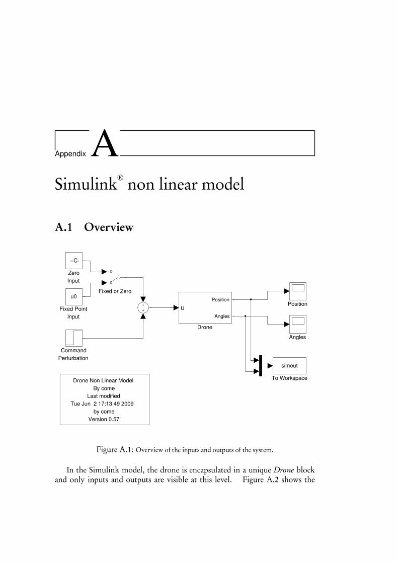
Figure A.1: Overview of the inputs and outputs of the system.
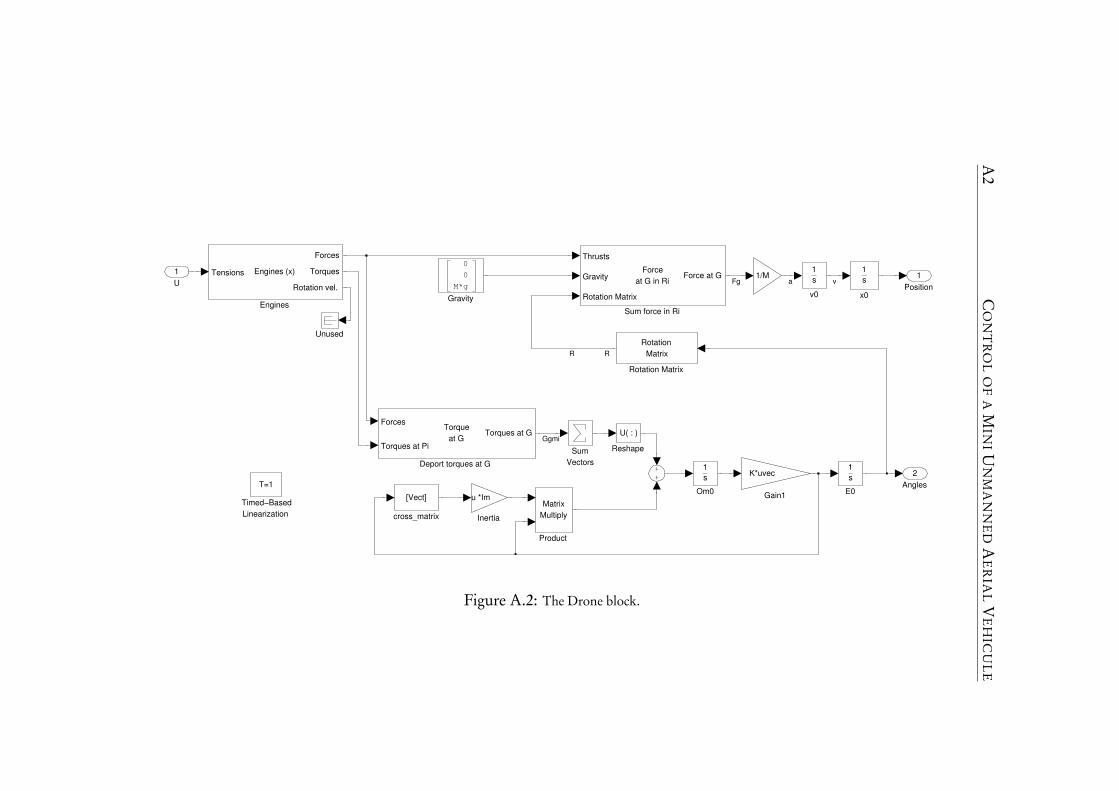
In the Simulink model, the drone is encapsulated in a unique Drone blockand only inputs and outputs are visible at this level. Figure A.2 shows the
A2
CO
NT
RO
LO
FA
MIN
IUN
MA
NN
ED
AE
RIA
LV
EH
ICU
LE
Angles
2
Position
1
x0
1
s
v0
1
s
cross_matrix
[Vect]
Unused
Timed−Based
Linearization
T=1
Sum force in Ri
Force
at G in Ri
Thrusts
Rotation Matrix
Gravity Force at G
Sum
Vectors
Rotation Matrix
Rotation
Matrix
Reshape
U( : )
Product
Matrix
Multiply
Om0
1
s
Inertia
u *Im
Gravity
0
0
M*g
Gain1
K*uvec
1/M
Engines
Engines (x)Tensions
Forces
Torques
Rotation vel.
E0
1
s
Deport torques at G
Torque
at G
Forces
Torques at Pi
Torques at G
U
1
vaFg
RR
Ggmi
Figure A.2: The Drone block.
SIMULINK® NON LINEAR MODEL A3
inside of the block. Inputs are directly fed to the Engines block that simulatesany number of engine independently (see figure A.3). Its output is split into twoparts. The upper part simulates acceleration, velocity and position while thelower part simulates the orientation and rotation speed.
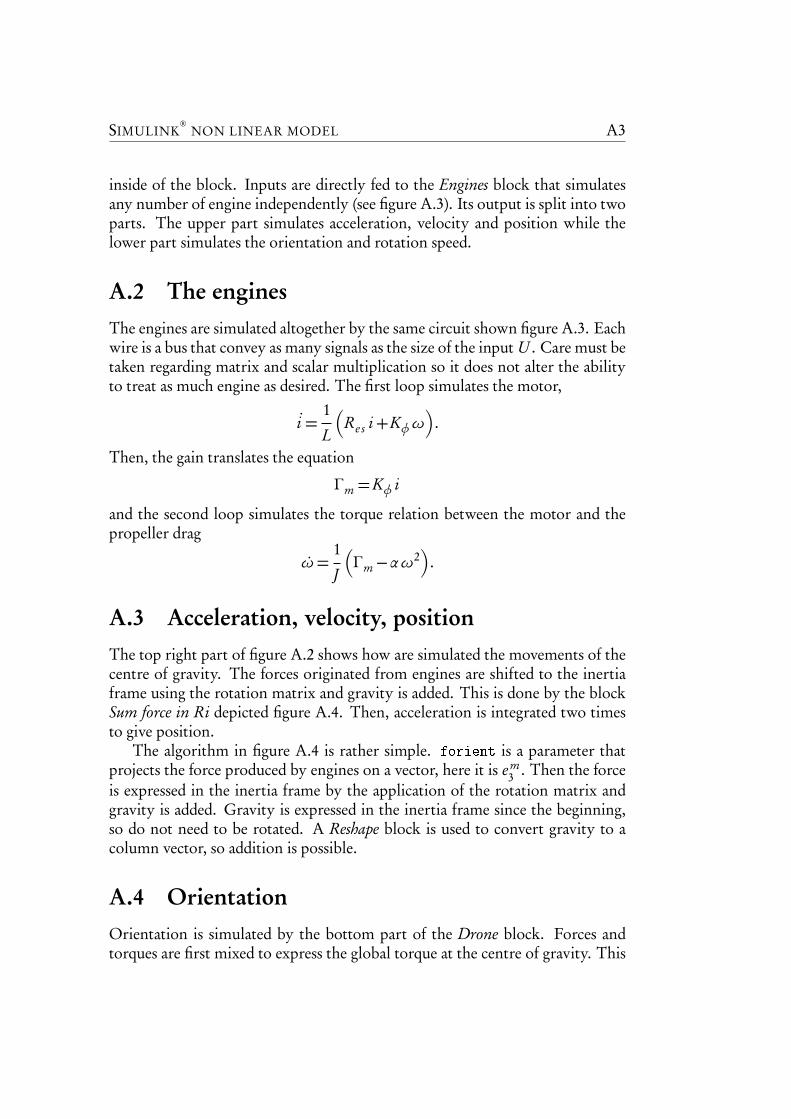
A.2 The enginesThe engines are simulated altogether by the same circuit shown figure A.3. Eachwire is a bus that convey as many signals as the size of the input U . Care must betaken regarding matrix and scalar multiplication so it does not alter the abilityto treat as much engine as desired. The first loop simulates the motor,
i =1
L
Re s i+Kφω
.
Then, the gain translates the equation
Γm =Kφ i
and the second loop simulates the torque relation between the motor and thepropeller drag
ω=1
J
Γm−αω2
.
A.3 Acceleration, velocity, positionThe top right part of figure A.2 shows how are simulated the movements of thecentre of gravity. The forces originated from engines are shifted to the inertiaframe using the rotation matrix and gravity is added. This is done by the blockSum force in Ri depicted figure A.4. Then, acceleration is integrated two timesto give position.
The algorithm in figure A.4 is rather simple. forient is a parameter thatprojects the force produced by engines on a vector, here it is e m
3 . Then the forceis expressed in the inertia frame by the application of the rotation matrix andgravity is added. Gravity is expressed in the inertia frame since the beginning,so do not need to be rotated. A Reshape block is used to convert gravity to acolumn vector, so addition is possible.
A.4 OrientationOrientation is simulated by the bottom part of the Drone block. Forces andtorques are first mixed to express the global torque at the centre of gravity. This
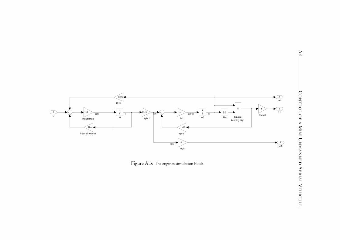
A4
CO
NT
RO
LO
FA
MIN
IUN
MA
NN
ED
AE
RIA
LV
EH
ICU
LE
wi
3
Gm
2
Ft
1
w0
1
s
alpha
−K−
Thrust
−k
Square
keeping signKphi i
Kphi
Kphi
Kphi
Internal resistor
Res
Inductance
1./L
I0
1
s
Gain
−1
Abs
|u|
1/J
1./J
U
1
i
i
Gm
Gm dot wi widot i
Figure A.3: The engines simulation block.
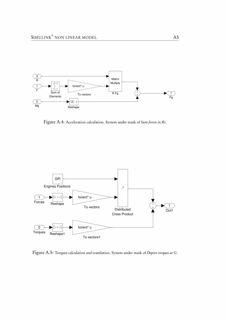
SIMULINK® NON LINEAR MODEL A5
Fg
1To vectors
forient* u
Sum of
Elements
Reshape
U( : )
R Fg
Matrix
MultiplyR
3
Mg
2
F
1
Figure A.4: Acceleration calculation. System under mask of Sum forces in Ri.
Out1
1
To vectors1
forient* u
To vectors
forient* u
Reshape1
Reshape
Engines Positions
GPi
Distributed
Cross Product
.^
Torques
2
Forces
1
Figure A.5: Torques calculation and translation. System under mask of Deport torques at G.
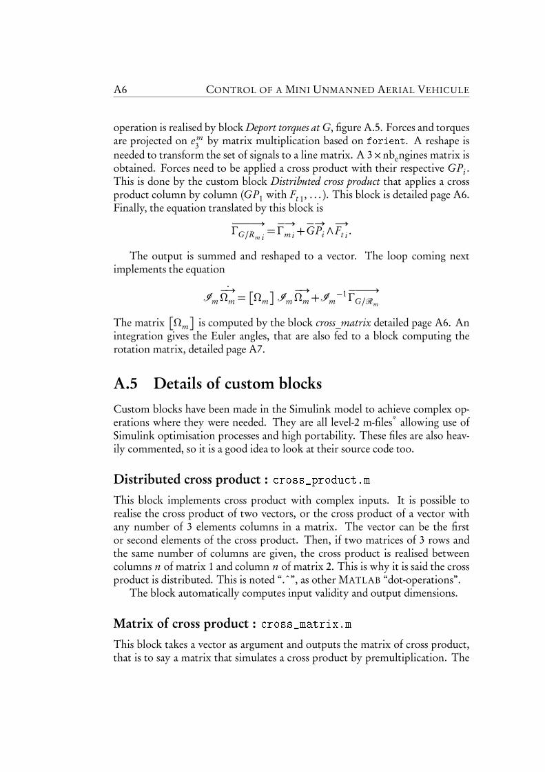
A6 CONTROL OF A MINI UNMANNED AERIAL VEHICULE
operation is realised by block Deport torques at G, figure A.5. Forces and torquesare projected on e m
3 by matrix multiplication based on forient. A reshape isneeded to transform the set of signals to a line matrix. A 3×nbengines matrix isobtained. Forces need to be applied a cross product with their respective GPi .This is done by the custom block Distributed cross product that applies a crossproduct column by column (GP1 with Ft 1, . . . ). This block is detailed page A6.Finally, the equation translated by this block is
−−−−→ΓG/Rm i
=−→Γm i+
−→GPi ∧
−→Ft i .
The output is summed and reshaped to a vector. The loop coming nextimplements the equation
Im−→Ωm =
Ωm
Im−→Ωm+Im
−1−−−→ΓG/Rm
The matrix
Ωm
is computed by the block cross_matrix detailed page A6. Anintegration gives the Euler angles, that are also fed to a block computing therotation matrix, detailed page A7.
A.5 Details of custom blocksCustom blocks have been made in the Simulink model to achieve complex op-erations where they were needed. They are all level-2 m-files* allowing use ofSimulink optimisation processes and high portability. These files are also heav-ily commented, so it is a good idea to look at their source code too.
Distributed cross product : cross_product.mThis block implements cross product with complex inputs. It is possible torealise the cross product of two vectors, or the cross product of a vector withany number of 3 elements columns in a matrix. The vector can be the firstor second elements of the cross product. Then, if two matrices of 3 rows andthe same number of columns are given, the cross product is realised betweencolumns n of matrix 1 and column n of matrix 2. This is why it is said the crossproduct is distributed. This is noted “.ˆ”, as other MATLAB “dot-operations”.
The block automatically computes input validity and output dimensions.
Matrix of cross product : cross_matrix.mThis block takes a vector as argument and outputs the matrix of cross product,that is to say a matrix that simulates a cross product by premultiplication. The
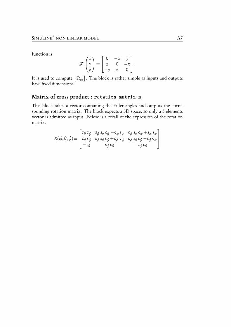
SIMULINK® NON LINEAR MODEL A7
function is
F
xyz
=
0 −z yz 0 −x−y x 0
.
It is used to compute
Ωm
. The block is rather simple as inputs and outputshave fixed dimensions.
Matrix of cross product : rotation_matrix.mThis block takes a vector containing the Euler angles and outputs the corre-sponding rotation matrix. The block expects a 3D space, so only a 3 elementsvector is admitted as input. Below is a recall of the expression of the rotationmatrix.
R(φ,θ,ψ)=
cθ cψ sφ sθ cψ−cφ sψ cφ sθ cψ+sφ sψcθ sψ sφ sθ sψ+cφ cψ cφ sθ sψ−sφ cψ−sθ sφ cθ cφ cθ

A8 CONTROL OF A MINI UNMANNED AERIAL VEHICULE
Appendix BMatlab code
B.1 Linearised model
File model.m1 % Establishes the model of the drone2
3 %%%%%%%%%%%%%%%%%%%%%%%%%%%%%%%%%%%%%%%%%%%%%%%%%%%%%%%%%%%%%%%%%%%%%%%%%%%%%%%%4 % Fixed point5 w0 = 200*2*pi/60 * [1,1,1,1]; % Rotation speed of motors6
7 % Euler angles at fixed point8 psi0 = 0; % Angle from inertia frame around e3 (applies on e'1 and e'2)9 th0 = 0; % Angle from inertia frame around e2 (applies on e'1 and e'3)
10 phi0 = 0; % Angle from inertia frame around e1 (applies on e'2 and e'3)11
12 % Angular velocity at fixed point13 Om0 = [ 0 ; 0 ; 0 ]; % According to em1,em2,em314
15 %%%%%%%%%%%%%%%%%%%%%%%%%%%%%%%%%%%%%%%%%%%%%%%%%%%%%%%%%%%%%%%%%%%%%%%%%%%%%%%%16 % General parameters17 nbe = 4; % Number of engines18 Mb = 0.250; % Body mass19 Mp = 0.01; % Propeller mass20 Mm = 0.04; % Motor mass21 l = 0.10 * [1,1,1,1]; % Propeller radius22 lm = 0.05 * [1,1,1,1]; % Motor radius23 hm = 0.05 * [1,1,1,1]; % Motor heights24 direction = [1,−1,1,−1]; % Engine rotation directions25
26 M = Mb+ nbe*(Mp + Mm); % Total mass27
28 % Position of engines from center of gravity of the model (in the mobile frame)29 r = 0.20; % Distance between an engine and the center of gravity30 % | GP1 | GP2 | GP3 | GP4 |31 GP = [ [ r , 0 , −r , 0 ] ; ...32 [ 0 , −r , 0 , r ] ; ...33 [ 0 , 0 , 0 , 0 ] ];34 % | GP1 | GP2 | GP3 | GP4 |35
36 % Parameters of engines
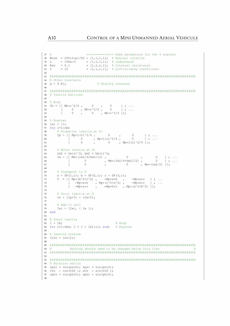
A10 CONTROL OF A MINI UNMANNED AERIAL VEHICULE
37 % −>|−−−−−−−|<−−− Same parameters for the 4 engines38 Wnom = 200*2*pi/60 * [1,1,1,1]; % Nominal rotation39 L = 100e−3 * [1,1,1,1]; % Inductance40 Res = 0.1 * [1,1,1,1]; % Internal resistance41 f = 10 * [1,1,1,1]; % Lift−to−drag coefficient42
43 %%%%%%%%%%%%%%%%%%%%%%%%%%%%%%%%%%%%%%%%%%%%%%%%%%%%%%%%%%%%%%%%%%%%%%%%%%%%%%%%44 % Other constants45 g = 9.81; % Gravity constant46
47 %%%%%%%%%%%%%%%%%%%%%%%%%%%%%%%%%%%%%%%%%%%%%%%%%%%%%%%%%%%%%%%%%%%%%%%%%%%%%%%%48 % Inertia matrices49
50 % Body51 Ib = [[ Mb*r^2/6 , 0 , 0 ] ; ...52 [ 0 , Mb*r^2/6 , 0 ] ; ...53 [ 0 , 0 , Mb*r^2/3 ]];54
55 % Engines56 Iei = ;57 for i=1:nbe58 % Propeller inertia at Pi59 Ip = [[ Mp*l(i)^2/4 , 0 , 0 ] ; ...60 [ 0 , Mp*l(i)^2/4 , 0 ] ; ...61 [ 0 , 0 , Mp*l(i)^2/4 ]];62
63 % Motor inertia at Pi64 lm2 = lm(i)^2; hm2 = hm(i)^2;65 Im = [[ Mm*(lm2/4+hm2/12) , 0 , 0 ] ; ...66 [ 0 , Mm*(lm2/4+hm2/12) , 0 ] ; ...67 [ 0 , 0 , Mm*(lm2/2) ]];68
69 % Transport to G70 a = GP(1,i); b = GP(2,i); c = GP(3,i);71 T = [[ Mp*(b^2+c^2) , −Mp*a*b , −Mp*a*c ] ; ...72 [ −Mp*a*b , Mp*(c^2+a^2) , −Mp*b*c ] ; ...73 [ −Mp*a*c , −Mp*b*c , Mp*(a^2+b^2) ]];74
75 % Total inertia at G76 Ie = (Ip+T) + (Im+T);77
78 % Add to cell79 Iei = [Iei, Ie ];80 end81
82 % Total inertia83 I = Ib; % Body84 for i=1:nbe; I = I + Ieii; end; % Engines85
86 % Inertia inverse87 Iinv = inv(I);88
89 %%%%%%%%%%%%%%%%%%%%%%%%%%%%%%%%%%%%%%%%%%%%%%%%%%%%%%%%%%%%%%%%%%%%%%%%%%%%%%%%90 % Nothing should need to be changed below this line %91 %%%%%%%%%%%%%%%%%%%%%%%%%%%%%%%%%%%%%%%%%%%%%%%%%%%%%%%%%%%%%%%%%%%%%%%%%%%%%%%%92
93 %%%%%%%%%%%%%%%%%%%%%%%%%%%%%%%%%%%%%%%%%%%%%%%%%%%%%%%%%%%%%%%%%%%%%%%%%%%%%%%%94 % Rotation matrix95 cpsi = cos(psi0); spsi = sin(psi0);96 cth = cos(th0 ); sth = sin(th0 );97 cphi = cos(phi0); sphi = sin(phi0);98
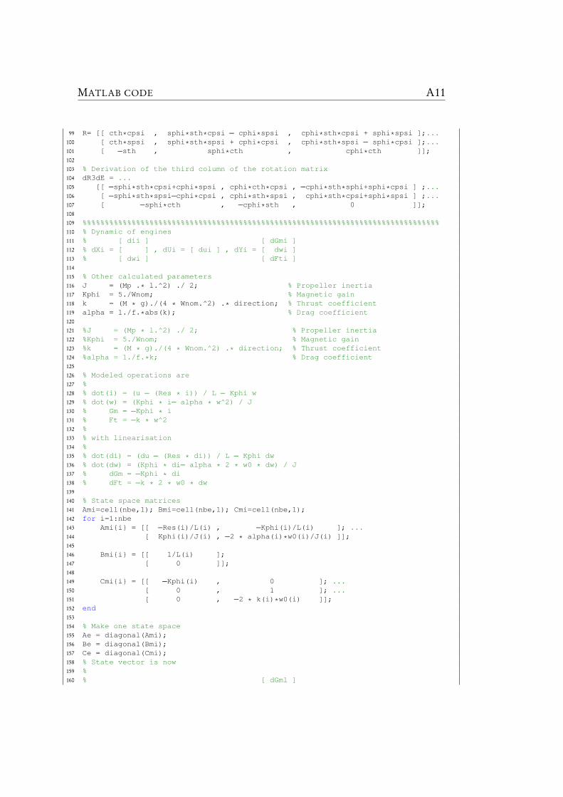
MATLAB CODE A11
99 R= [[ cth*cpsi , sphi*sth*cpsi − cphi*spsi , cphi*sth*cpsi + sphi*spsi ];...100 [ cth*spsi , sphi*sth*spsi + cphi*cpsi , cphi*sth*spsi − sphi*cpsi ];...101 [ −sth , sphi*cth , cphi*cth ]];102
103 % Derivation of the third column of the rotation matrix104 dR3dE = ...105 [[ −sphi*sth*cpsi+cphi*spsi , cphi*cth*cpsi , −cphi*sth*sphi+sphi*cpsi ] ;...106 [ −sphi*sth*spsi−cphi*cpsi , cphi*sth*spsi , cphi*sth*cpsi+sphi*spsi ] ;...107 [ −sphi*cth , −cphi*sth , 0 ]];108
109 %%%%%%%%%%%%%%%%%%%%%%%%%%%%%%%%%%%%%%%%%%%%%%%%%%%%%%%%%%%%%%%%%%%%%%%%%%%%%%%%110 % Dynamic of engines111 % [ dii ] [ dGmi ]112 % dXi = [ ] , dUi = [ dui ] , dYi = [ dwi ]113 % [ dwi ] [ dFti ]114
115 % Other calculated parameters116 J = (Mp .* l.^2) ./ 2; % Propeller inertia117 Kphi = 5./Wnom; % Magnetic gain118 k = (M * g)./(4 * Wnom.^2) .* direction; % Thrust coefficient119 alpha = 1./f.*abs(k); % Drag coefficient120
121 %J = (Mp * l.^2) ./ 2; % Propeller inertia122 %Kphi = 5./Wnom; % Magnetic gain123 %k = (M * g)./(4 * Wnom.^2) .* direction; % Thrust coefficient124 %alpha = 1./f.*k; % Drag coefficient125
126 % Modeled operations are127 %128 % dot(i) = (u − (Res * i)) / L − Kphi w129 % dot(w) = (Kphi * i− alpha * w^2) / J130 % Gm = −Kphi * i131 % Ft = −k * w^2132 %133 % with linearisation134 %135 % dot(di) = (du − (Res * di)) / L − Kphi dw136 % dot(dw) = (Kphi * di− alpha * 2 * w0 * dw) / J137 % dGm = −Kphi * di138 % dFt = −k * 2 * w0 * dw139
140 % State space matrices141 Ami=cell(nbe,1); Bmi=cell(nbe,1); Cmi=cell(nbe,1);142 for i=1:nbe143 Amii = [[ −Res(i)/L(i) , −Kphi(i)/L(i) ]; ...144 [ Kphi(i)/J(i) , −2 * alpha(i)*w0(i)/J(i) ]];145
146 Bmii = [[ 1/L(i) ];147 [ 0 ]];148
149 Cmii = [[ −Kphi(i) , 0 ]; ...150 [ 0 , 1 ]; ...151 [ 0 , −2 * k(i)*w0(i) ]];152 end153
154 % Make one state space155 Ae = diagonal(Ami);156 Be = diagonal(Bmi);157 Ce = diagonal(Cmi);158 % State vector is now159 %160 % [ dGm1 ]
A12 CONTROL OF A MINI UNMANNED AERIAL VEHICULE
161 % [ dw1 ]162 % [ di1 ] [ dFt1 ]163 % [ dw1 ] [ dGm2 ]164 % [ di2 ] [ du1 ] [ dw2 ]165 % dX = [ dw2 ] , dU = [ du2 ] , dY = [ dFt2 ]166 % [ di3 ] [ du3 ] [ dGm3 ]167 % [ dw3 ] [ du4 ] [ dw3 ]168 % [ di4 ] [ dFt3 ]169 % [ dw4 ] [ dGm4 ]170 % [ dw4 ]171 % [ dFt4 ]172
173 %%%%%%%%%%%%%%%%%%%%%%%%%%%%%%%%%%%%%%%%%%%%%%%%%%%%%%%%%%%%%%%%%%%%%%%%%%%%%%%%174 % Action of force on position175 Fti = Ce(3:3:(nbe*3),:); % Get Ft according to w176 CFtl = ones(1,nbe) * Fti; % Sum forces for each engine177 % Convert to inertia frame but keep only relevant part of rotation matrix178 % as Ft is expressed only according to em3 and add gravity.179 Fg = [[ R(1,3) .* CFtl ] ; ...180 [ R(2,3) .* CFtl ] ; ...181 [ R(3,3) .* CFtl ]];182 Ag = Fg./M;183
184 % Calculates action of angles on acceleration185 % Compute resultant force at fixed point186 Ft0 = 0;187 for i=1:nbe188 Ft0 = Ft0 − abs(k(i))*(w0(i)^2);189 end190 AEa = 1/M * dR3dE * Ft0;191
192 % Include system velocity inside state space193 % dot(v) = Fg/M194 Av = [[ Ae , zeros(size(Ae,1),3) ] ; ...195 [ Ag , zeros(3,3) ]];196
197 Bv = [[ Be ] ; ...198 [ zeros(3, size(Be,2)) ]];199
200 Cv = [ Ce , zeros(size(Ce,1),3) ] ;201
202 % Include system position inside state space203 % dot(p) = v204 Ap = [[ Av , zeros(size(Av,1),3) ] ;...205 [ zeros(3,size(Av,2)−3) , diag([1, 1, 1]) , zeros(3,3) ]];206
207 Bp = [[ Bv ] ; ...208 [ zeros(3, size(Bv,2)) ]];209
210 Cp = diagonal( Cv , diag([1, 1, 1]) );211
212 % State vector is now213 %214 % [ i1 ] [ Gm1 ]215 % [ w1 ] [ w1 ]216 % [ i2 ] [ Ft1 ]217 % [ w2 ] [ Gm2 ]218 % [ i3 ] [ w2 ]219 % [ w3 ] [ Ft2 ]220 % [ i4 ] [ u1 ] [ Gm3 ]221 % X = [ w4 ] , U = [ u2 ] , Y = [ w3 ]222 % [ vx ] [ u3 ] [ Ft3 ]
MATLAB CODE A13
223 % [ vy ] [ u4 ] [ Gm4 ]224 % [ vz ] [ w4 ]225 % [ x ] [ Ft4 ]226 % [ y ] [ x ]227 % [ z ] [ y ]228 % [ z ]229
230 %%%%%%%%%%%%%%%%%%%%%%%%%%%%%%%%%%%%%%%%%%%%%%%%%%%%%%%%%%%%%%%%%%%%%%%%%%%%%%%%231 % Action of torques on orientation232
233 % Modeled equations are234 %235 % dot(Omega) = −I^(−1) * Mom * I * Omega + I^(−1) * Ggr236 % Ggr = Sum(Gmi + GPi ^ Fti )237 %238 % We neglect gyroscopic torques.239
240 % Get Gm and project on em3241 Gm = [[ zeros(2, size(Ce,2)) ] ; ...242 [ ones(1,nbe) * Ce(1:3:(nbe*3),:) ]];243
244 % Create matrix to do vectorial product245 GPm = [[ GP(2,:) ] ; ...246 [ −GP(1,:) ] ; ...247 [ zeros(1,size(GP,2)) ]];248
249 % General torque at G (according to i and w)250 Ggr = (Gm + GPm * Fti);251 Aoe = Iinv * Ggr;252
253 %%%%%%%%%%%%%%%%%%%%%%%%%%%%%%%%%%%%%%%%%%%%%%%%%%%%%%%%%%%%%%%%%%%%%%%%%%%%%%%%254 % Action on orientation velocity on orientation255
256 % Matrix of the rotational velocity vector257 Mom = [[ 0 , −Om0(3) , Om0(2) ] ; ...258 [ Om0(3) , 0 , −Om0(1) ] ; ...259 [ −Om0(2) , Om0(1) , 0 ]];260
261 % First part of Om according to dOm262 AOm0 = Iinv * Mom * I;263
264 % Extraction of dOm from [dOm]265
266 % Definitions267 wx = Om0(1);268 wy = Om0(2);269 wz = Om0(3);270
271 A = I(1,1);272 B = I(2,2);273 C = I(3,3);274 D = −I(1,3);275 E = −I(2,3);276 F = −I(1,2);277
278 % Inversion denominator279 alpha = 1/(C*F^2 + 2*D*E*F + B*E^2 + A*D^2 + A*B*C);280
281 % Coefficient matrix282 m11 = wx * (D*F^2 − C*E*F + B*E*F − D*E^2 ) ...283 −wy * (C*D*F + B*D*F + D^2*E + B^2*E) ...284 +wz * (D^2*F + C^2*F + C*D*E + B*D*E);
A14 CONTROL OF A MINI UNMANNED AERIAL VEHICULE
285 m12 = wx * (A*D*F − D^2*E + B*C*E + A*B*E) ...286 −wy * (D*F^2 + B*E*F + D^3 − B*C*D) ...287 −wz * (D*E*F + B*E^2 − C*D^2 + B*C^2);288 m13 = wx * (D^2*F − B*C*F − A*C*F − A*D*E) ...289 +wy * (C*F^2 + D*E*F − B*D^2 + B^2*C) ...290 +wz * (C*E*F + D*E^2 + D^3 − B*C*D);291 m21 = wx * (E*F^2 + A*D*F + E^3 − A*C*E) ...292 −wy * (B*E*F − D*E^2 + A*C*D + A*B*D) ...293 +wz * (D*E*F − C*E^2 + A*D^2 + A*C^2);294 m22 = wx * (C*E*F + A*E*F + D*E^2 + A^2*D) ...295 −wy * (E*F^2 − C*D*F + A*D*F − D^2*E) ...296 −wz * (E^2*F + C^2*F + C*D*E + A*D*E);297 m23 = −wx * (C*F^2 + D*E*F − A*E^2 + A^2*C) ...298 −wy * (E^2*F − B*C*F − A*C*F − B*D*E) ...299 −wz * (C*D*F + E^3 + D^2*E − A*C*E);300 m31 = −wx * (F^3 + E^2*F − A*B*F + A*D*E) ...301 +wy * (B*F^2 − D*E*F − A*D^2 − A*B^2) ...302 −wz * (D*F^2 − C*E*F − A*C*D − A*B*D);303 m32 = −wx * (A*F^2 − D*E*F − B*E^2 − A^2*B) ...304 +wy * (F^3 + D^2*F − A*B*F + B*D*E) ...305 +wz * (E*F^2 − C*D*F − B*C*E − A*B*E);306 m33 = −wx * (D*F^2 + B*E*F + A*E*F + A^2*D) ...307 +wy * (E*F^2 + B*D*F + A*D*F + B^2*E) ...308 +wz * (E^2*F − D^2*F − B*D*E + A*D*E);309
310 M0 = [[m11, m12, m13] ; ...311 [m21, m22, m23] ; ...312 [m31, m32, m33]];313
314 AOm = AOm0 + alpha * M0;315
316 % Aga has 3 lines because GPi are expressed in 3D317 % That matches with the 3 angular accelerations318 Aav = [[ Ap , zeros(size(Ap,1),3) ] ; ...319 [ Aoe , zeros( 3 , size(Ap,2)−size(Aoe,2) ) , AOm ]];320
321 Bav = [[ Bp ] ; ...322 [ zeros( 3 , size(Bp,2) ) ]];323
324 Cav = [ Cp , zeros( size(Cp,1) , 3 ) ];325
326 % Include system angular position inside state space327 % dot(angle) = Omega328 AEaav = [[ zeros(size(Ae,1),3) ] ; ...329 [ AEa ] ; ...330 [ zeros(6,3) ]];331
332 Aa = [[ Aav , AEaav ] ;...333 [ zeros(3,size(Aav,2)−3) , diag([1, 1, 1]) , zeros(3,3) ]];334
335 Ba = [[ Bav ] ; ...336 [ zeros(3, size(Bav,2)) ]];337
338 Ca = diagonal( Cav , diag([1, 1, 1]) );339
340 % State vector is now341 %342 % [ i1 ]343 % [ w1 ] [ Gm1 ]344 % [ i2 ] [ w1 ]345 % [ w2 ] [ Ft1 ]346 % [ i3 ] [ Gm2 ]
MATLAB CODE A15
347 % [ w3 ] [ w2 ]348 % [ i4 ] [ Ft2 ]349 % [ w4 ] [ Gm3 ]350 % [ vx ] [ u1 ] [ w3 ]351 % X = [ vy ] , U = [ u2 ] , Y = [ Ft3 ]352 % [ vz ] [ u3 ] [ Gm4 ]353 % [ x ] [ u4 ] [ w4 ]354 % [ y ] [ Ft4 ]355 % [ z ] [ x ]356 % [ Omx ] [ y ]357 % [ Omy ] [ z ]358 % [ Omz ] [ phi ]359 % [ phi ] [ th ]360 % [ th ] [ psi ]361 % [ psi ]362 %363 % With Om? the angular velocity in mobile frame364 % and phi, th, psi the Euler angles.365
366 %%%%%%%%%%%%%%%%%%%%%%%%%%%%%%%%%%%%%%%%%%%%%%%%%%%%%%%%%%%%%%%%%%%%%%%%%%%%%%%%367 % Reduction of outputs368
369 A = Aa;370 B = Ba;371
372 f = size(Ca,1); % Last line index373 C = Ca(f−5:f , :); % Only keep the last six lines374
375 % State vector is now376 %377 % [ i1 ]378 % [ w1 ]379 % [ i2 ]380 % [ w2 ]381 % [ i3 ]382 % [ w3 ]383 % [ i4 ]384 % [ w4 ] [ x ]385 % [ vx ] [ u1 ] [ y ]386 % X = [ vy ] , U = [ u2 ] , Y = [ z ]387 % [ vz ] [ u3 ] [ phi ]388 % [ x ] [ u4 ] [ th ]389 % [ y ] [ psi ]390 % [ z ]391 % [ Omx ]392 % [ Omy ]393 % [ Omz ]394 % [ phi ]395 % [ th ]396 % [ psi ]397 %398
399 %%%%%%%%%%%%%%%%%%%%%%%%%%%%%%%%%%%%%%%%%%%%%%%%%%%%%%%%%%%%%%%%%%%%%%%%%%%%%%%%

A16 CONTROL OF A MINI UNMANNED AERIAL VEHICULE
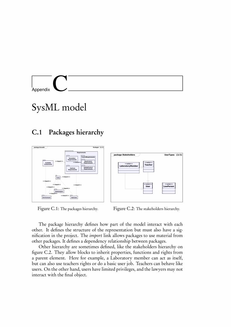
Appendix CSysML model
C.1 Packages hierarchy
package Drone01 Packages 1/1
Stakeholders
Requirements
SecundaryRequirements
ControlRequirements
BaseControlRequirements
EmbedControlRequirements
UseCaseRequirements
Tools
<<import>>
<<import>>
<<import>>
UseCases
<<import>>
<<import>>
Environment
<<import>>
<<import>>
<<import>>
AvailableComponents
<<import>>
<<import>>
Figure C.1: The packages hierarchy.
package Stakeholders UserTypes 2/2
<<actor>>
Teacher
<<actor>>
User
<<actor>>
LawPerson
<<actor>>
LaboratoryMember
Figure C.2: The stakeholders hierarchy.
The package hierarchy defines how part of the model interact with eachother. It defines the structure of the representation but must also have a sig-nification in the project. The import link allows packages to use material fromother packages. It defines a dependency relationship between packages.
Other hierarchy are sometimes defined, like the stakeholders hierarchy onfigure C.2. They allow blocks to inherit properties, functions and rights froma parent element. Here for example, a Laboratory member can act as itself,but can also use teachers rights or do a basic user job. Teachers can behave likeusers. On the other hand, users have limited privileges, and the lawyers may notinteract with the final object.
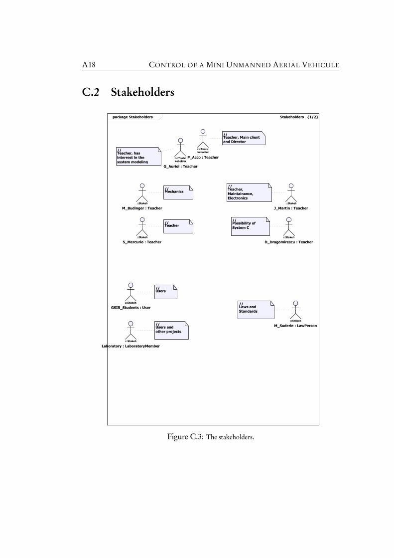
A18 CONTROL OF A MINI UNMANNED AERIAL VEHICULE
C.2 Stakeholders
package Stakeholders Stakeholders 1/2
G_Auriol : Teacher
<<Tools::Stakeholder
P_Acco : Teacher
<<Tools::Stakeholder
GSI5_Students : User
Tools::Stakeholder
//Teacher, has
interrest in the
system modeling
//Teacher, Main client
and Director
//Users
M_Budinger : Teacher
Tools::Stakeholder
//Mechanics
S_Mercurio : Teacher
Tools::Stakeholder
//Teacher
J_Martin : Teacher
Tools::Stakeholder
//Teacher,
Maintainance,
Electronics
D_Dragomirescu : Teacher
Tools::Stakeholder
//Possibility of
System C
M_Suderie : LawPerson
Tools::Stakeholder
//Laws and
Standards
Laboratory : LaboratoryMember
Tools::Stakeholder
//Users and
other projects
Figure C.3: The stakeholders.
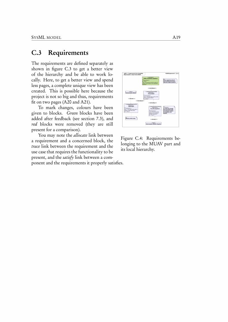
SYSML MODEL A19
C.3 Requirements
public <<requirement,Tools::Useability
Requirement>>class 'Drone MUAV'
MUAVRequirement 1/1
«»
<<requirement,Tools::UseabilityRequirement>>
'Drone MUAV'
<<requirement>>Text = "The final object will be a Mini Unmanned Aerial Vehicle"Id = "Use.4"
«»
<<requirement,Tools::ConstraintRequirement>>
Lightweight
<<requirement>>Text = "The object will be light in weight to allow easy flying"Id = "Func.2"
//Missing units/range
«»
<<requirement,Tools::ConstraintRequirement>>
'Fly with propellers'
<<requirement>>Text = "The drone will be operated by an unknown number of propellers"Id = "Func.3"
//
A model has already
been described with
an unknown number
of propellers and
motors
<<rationale>>
<<deriveReqt>>
<<deriveReqt>>
<<block>>
Environment::MUAV::Propeller
<<block>>
Environment::MUAV
<<allocate>>
<<allocate>>
«»
<<requirement>>
'Satify realisability equations'
<<requirement>>Id="Ctrl.3"Text="The structure and the number of engines must comply to the realisability equations"
<<deriveReqt>>
//These equations state if
the considered structure
will have stable positions
Figure C.4: Requirements be-longing to the MUAV part andits local hierarchy.
The requirements are defined separately asshown in figure C.3 to get a better viewof the hierarchy and be able to work lo-cally. Here, to get a better view and spendless pages, a complete unique view has beencreated. This is possible here because theproject is not so big and thus, requirementsfit on two pages (A20 and A21).
To mark changes, colours have beengiven to blocks. Green blocks have beenadded after feedback (see section 7.3), andred blocks were removed (they are stillpresent for a comparison).
You may note the allocate link betweena requirement and a concerned block, thetrace link between the requirement and theuse case that requires the functionality to bepresent, and the satisfy link between a com-ponent and the requirements it properly satisfies.
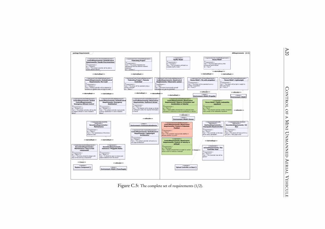
A20
CO
NT
RO
LO
FA
MIN
IUN
MA
NN
ED
AE
RIA
LV
EH
ICU
LE
package Requirements
«»
<<requirement,FunctionalityRequirement>>
ControlRequirements::EmbedControl
Requirements::'Emergency
Stabilisation'
<<requirement>>Id = "Embed.2.1.1"Text = "The embed controller must provide null-trim stabilization in case of datalink failure"
«»
<<requirement,FunctionalityRequirement>>
ControlRequirements::Embed
ControlRequirements::
'Emergency Altitude Control'
<<requirement>>Id = "Embed.2.1.2"Text = "The embed controller will be able to stabilize altitude in case of datalink failure"
«»
<<requirement,Tools::ConstraintRequirement>>
'Federating Project'
<<requirement>>Text = "The project federates two laboratories that has different research objectives"Id = "Context.1"
«»
<<requirement,Tools::FunctionalityRequirement>>
'Federating Project'::'Remote
Controlled'
<<requirement>>Text = "The drone will be operated using a remote controller"Id = "Basic.1"
«»
<<requirement,Tools::UseabilityRequirement>>
SecundaryRequirements::
Maintainance
<<requirement>>Id = "Maint.1"Text = "The maintainance of the drone should be easy"
«»
<<requirement>>
SecundaryRequirements::
Maintainance::'Pluggable Batteries'
<<requirement>>Id = "Maint.1.1"Text = "It should be easy to remove and replace batteries from the drone"
«»
<<requirement,ConstraintRequirement>>
SecundaryRequirements::
Maintainance::'Easy to find
components'
<<requirement>>Id = "Maint.1.2"Text = "The drone should be design with easy to find and buy components"
«»
<<requirement,Tools::ConstraintRequirement>>
ControlRequirements::BaseControl
Requirements::'Sufficient bitrate'
<<requirement>>Id = "Func.1.3"Text = "The datalink will be design so bitrate is sufficient to allow the required information to transit"
«»
<<requirement,Tools::FunctionalityRequirement>>
ControlRequirements::EmbedControl
Requirements::'Handle Disconnections'
<<requirement>>Id = "Embed.2"Text = "The embed controller will be able to handle datalink failures"
«»
<<requirement,Tools::ConstraintRequirement>>
ControlRequirements::EmbedControl
Requirements::'Lightweight
Architecture'
<<requirement>>Id = "Embed.1"Text = "The embed controller will work on a very light architecture"
«»
<<requirement
ControlRequirements
Requirements::'Observab
<<requirementId = "Ctrl.1"Text = "The drone must provide enough information so it can be cont
«»
<<requirement,Tools::ReliabilityRequirement>>
ControlRequirements::EmbedControl
Requirements::'No Crash'
<<requirement>>Id = "Embed.2.1"Text = "Embed controller will be designed so problems on datalink does not lead to crash"
<<deriveReqt>><<deriveReqt>>
<<deriveReqt>>
<<deriveReqt>>
<<deriveReqt>><<deriveReqt>>
<<deriveReqt
<<deriveReqt>>
<<usecase>>
'Replace Component'()
<<trace>>
<<block>>
Environment::MUAV::PowerSupply
<<block>>
Environment::CommunicationDevice
<<allocate>>
<<allocate>>
AllRequirements 2/2
«»
<<requirement,FunctionalityRequirement>>
UseCaseRequirements::
'Changeable BaseController'
<<requirement>>Id = "Func.5"Text = "The controller on the base will be easily uploadable"
«»
<<requirement>>
UseCaseRequirements::'Base
Controller Host'
<<requirement>>Id = "Func.5.1"Text = "The controller host will be generic"
«»
<<requirement,Tools::UseabilityRequirement>>
'Drone MUAV'
<<requirement>>Text = "The final object will be a Mini Unmanned Aerial Vehicle"Id = "Use.4"
«»
<<requirement,Tools::ConstraintRequirement>>
SecundaryRequirements::'A3
Size'
<<requirement>>Id = "Use.5"Text = "The drone will have to fit in a A3 (297 × 420) paper area"
«»
<<requirement,Tools::ConstraintRequirement>>
'Drone MUAV'::'Fly with propellers'
<<requirement>>Text = "The drone will be operated by an unknown number of propellers"Id = "Func.3"
«»
<<requirement>>
'SysML Model'
<<requirement>>Id = "Concept.1"Text = "The conception will lead to a complete SysML model."
«»
<<requirement,FunctionalityRequirement>>
ControlRequirements::BaseControl
Requirements::'Control of Absolute
Position'
<<requirement>>Id = "Ctrl.2"Text = "The controller must provide stability in absolute position (x,y,z,th)"
requirement,Tools::FunctionalityRequirement>>
ControlRequirements::BaseControl
Requirements::'Observable system'
requirement>>"Ctrl.1""The drone must provide enough
information so it can be controlled"
«»
<<requirement,Tools::ConstraintRequirement>>
'Drone MUAV'::Lightweight
<<requirement>>Text = "The object will be light in weight to allow easy flying"Id = "Func.2"
<<deriveReqt>>
<<deriveReqt>><<deriveReqt>>
deriveReqt>>
<<usecase>>
'Upload Controller on Base'()
<<trace>>
<<block>>
Environment::MUAV
<<block>>
Environment::MUAV::Propeller
«»
<<requirement>>
ControlRequirements::BaseControl
Requirements::'Control of velocity or
attitude'
<<requirement>>Id = "Ctrl.2mod"Text = "Studies showed that it is easier to control drone in term of velocity or attitude"
«»
<<requirement,ConstraintRequirement>>
ControlRequirements::BaseControl
Requirements::'Observe Orientation and
Acceleration or Velocity'
<<requirement>>Id = "Ctrl.1.1"Text = "Observability showed that it is achieved when orientation is observed as well as acceleration or velocity."
<<deriveReqt>>
<<block>>
Environment::MUAV::Sensor
<<allocate>>
<<allocate>> <<allocate>>
«»
<<requirement>>
'Drone MUAV'::'Satify realisability
equations'
<<requirement>>Id = "Ctrl.3"Text = "The structure and the number of engines must comply to the realisability equations"
<<deriveReqt>>
<<allocate>>
Figure C.5: The complete set of requirements (1/2).
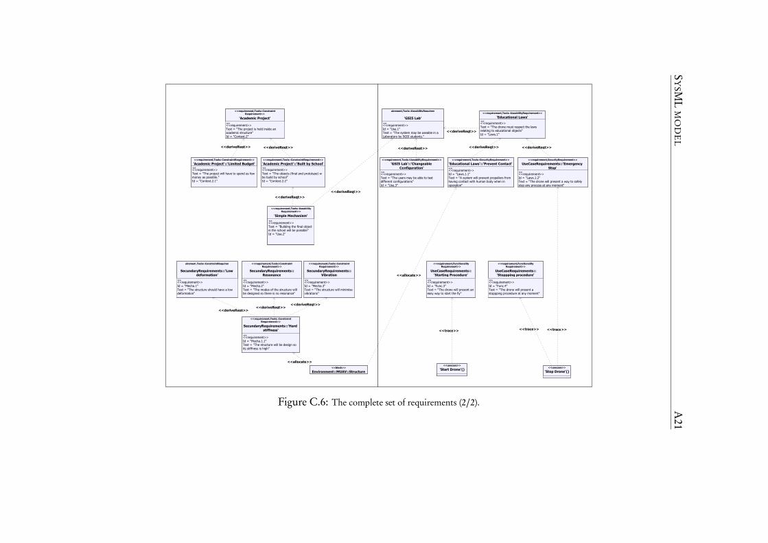
SY
SML
MO
DE
LA
21
«»
<<requirement,Tools::UseabilityRequirement>>
'Simple Mechanism'
<<requirement>>Text = "Building the final object in the school will be possible"Id = "Use.2"
«»
<<requirement,Tools::ConstraintRequirement>>
'Academic Project'
<<requirement>>Text = "The project is held inside an academic structure"Id = "Context.2"
«»
<<requirement,Tools::ConstraintRequirement>>
'Academic Project'::'Limited Budget'
<<requirement>>Text = "The project will have to spend as few money as possible."Id = "Context.2.1"
«»
<<requirement,Tools::ConstraintRequirement>>
'Academic Project'::'Built by School'
<<requirement>>Text = "The objects (final and prototype) will be build by school"Id = "Context.2.2"
«»
requirement,Tools::ConstraintRequirement
SecundaryRequirements::'Low
deformation'
<<requirement>>Id = "Mecha.1"Text = "The structure should have a low deformation"
«»
<<requirement,Tools::ConstraintRequirement>>
SecundaryRequirements::
Resonance
<<requirement>>Id = "Mecha.2"Text = "The modes of the structure will be designed so there is no resonance"
«»
<<requirement,Tools::ConstraintRequirement>>
SecundaryRequirements::
Vibration
<<requirement>>Id = "Mecha.3"Text = "The structure will minimise vibrations"
«»
<<requirement,Tools::ConstraintRequirement>>
SecundaryRequirements::'Hard
stiffness'
<<requirement>>Id = "Mecha.1.1"Text = "The structure will be design so its stiffness is high"
<<deriveReqt>>
<<deriveReqt>>
<<deriveReqt>> <<deriveReqt>>
<<deriveReqt>><<deriveReqt>>
<<deriveReqt>>
<<block>>
Environment::MUAV::Structure
<<allocate>>
«»
<<requirement,Tools::SecurityRequirement>>
'Educational Laws'::'Prevent Contact'
<<requirement>>Id = "Laws.1.1"Text = "A system will prevent propellers from having contact with human body when in operation"
«»
<<requirement,FunctionalityRequirement>>
UseCaseRequirements::
'Starting Procedure'
<<requirement>>Id = "Func.3"Text = "The drone will present an easy way to start the fly"
«»
<<requirement,FunctionalityRequirement>>
UseCaseRequirements::
'Stoppping procedure'
<<requirement>>Id = "Func.4"Text = "The drone will present a stoppping procedure at any moment"
«»
<<requirement,SecurityRequirement>>
UseCaseRequirements::'Emergency
Stop'
<<requirement>>Id = "Laws.1.2"Text = "The drone will present a way to safely stop any process at any moment"
«»
requirement,Tools::UseabilityRequirement
'GSI5 Lab'
<<requirement>>Id = "Use.1"Text = "The system may be useable in a Laboratory by 5GSI students."
«»
<<requirement,Tools::UseabilityRequirement>>
'GSI5 Lab'::'Changeable
Configuration'
<<requirement>>Text = "The users may be able to test different configurations"Id = "Use.3"
«»
<<requirement,Tools::UseabilityRequirement>>
'Educational Laws'
<<requirement>>Text = "The drone must respect the laws relating to educational objects"Id = "Laws.1"
<<deriveReqt>> <<deriveReqt>><<deriveReqt>>
<<deriveReqt>>
<<usecase>>
'Stop Drone'()
<<trace>> <<trace>>
<<usecase>>
'Start Drone'()
<<trace>>
<<allocate>>
Figure C.6: The complete set of requirements (2/2).
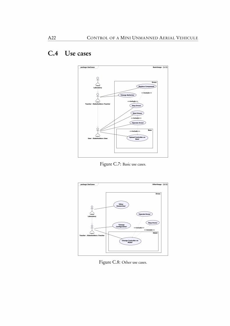
A22 CONTROL OF A MINI UNMANNED AERIAL VEHICULE
C.4 Use cases
package UseCases BasicUsage 1/2
Base
Drone
'Start Drone'
'Upload Controller on
Base'
'Operate Drone'
<<include>>
<<include>>
Teacher : Stakeholders::Teacher
<<actor>>
User : Stakeholders::User
<<actor>>
'Stop Drone'
'Change Batteries'
<<include>>
'Replace Component'
<<include>>
Laboratory
Tools::Stakeholder
Figure C.7: Basic use cases.
package UseCases OtherUsage 2/2
MUAV
Drone
Teacher : Stakeholders::Teacher
<<actor>>
'Change
Configuration'
'Other
Researches'
'Change Controller on
MUAV'
'Operate Drone'
<<include>>
'Stop Drone'
<<include>>
Laboratory
Tools::Stakeholder
Figure C.8: Other use cases.
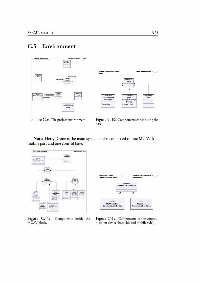
SYSML MODEL A23
C.5 Environment
package Environment GlobalEnvironment 1/1
<<block>>
Drone
<<block>>
Base
1
<<block>>
MUAV
1
<<actor>>
User
Commands
<<actor>>
Teacher
Maintainance
<<block>>
Environment
Turbulences
<<block>>
Communication
Device
PhysicalValues
Movement
Figure C.9: The project environment.
active <<block>>class
Base
BaseComponents 1/1
<<block>>
Base
<<block>>
BaseCalculation
Plateform
+ ops : Real
<<block>>
Base
Communication
Device
+ bitrate : Real
<<block>>
IHM
1
1
1
Figure C.10: Components constituting thebase.
Note: Here, Drone is the main system and is composed of one MUAV (themobile part and one control base.
active <<block>>class MUAV MUAVComponents 1/2
<<block>>
MUAV
<<block>>
Structure
+ mass : Real
+ centerOfInertia : Tools::Point
+ ssize : Tools::Solid
+ price : Real
1
<<block>>
Rotor
1..*
<<block>>
Engine
+ couple : Real
+ mass : Real
+ power : Real
+ ssize : Tools::Solid
+ price : Real
<<block>>
Propeller
+ diameter : Real
+ pitch : Real
+ mass : Real
+ price : Real
1
1
<<block>>
Intelligence
1
<<block>>
Embed
Calculation
Plateform
+ mass : Real
+ ssize : Tools::Solid
+ ops : Real
+ price : Real
<<block>>
Embed
Communication
Device
+ mass : Real
+ ssize : Tools::Solid
+ bitrate : Real
+ price : Real
1
1
<<block>>
Reducer
+ factor : Real
+ mass : Real
+ price : Real
0..1
<<block>>
PowerSupply
+ voltage : Real
+ autonomy : Real
+mass : Real
+ price : Real
1
<<block>>
Embed
Controller
1
<<block>>
Sensor
+ physicalValue : String
+ mass : Real
+ price : Real
+ precision : Real
0..*
Figure C.11: Components inside theMUAV block.
<<block>>class
CommunicationDevice
CommunicationDevice
Components
1/1
<<block>>
CommunicationDevice
<<block>>
MUAV::Embed
CommunicationDevice
<<block>>
Base::Base
CommunicationDevice
1
1
Figure C.12: Components of the commu-nication device (base side and mobile side).
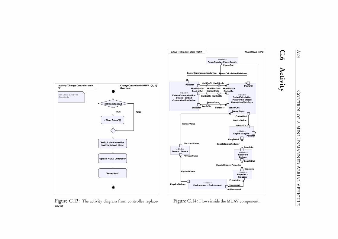
A24
CO
NT
RO
LO
FA
MIN
IUN
MA
NN
ED
AE
RIA
LV
EH
ICU
LE
C.6
Activityactivity 'Change Controller on MUA
V'
ChangeControllerOnMUAV
Overview
1/1
isDroneStopped
Boolean isDroneStopped;
: 'Stop Drone'()
True
'Switch the Controller
Host In Upload Mode'
False
'Upload MUAV Controller'
'Reset Host'
Figure C.13: The activity diagram from controller replace-ment.
active <<block>>class MUAV MUAVFlows 2/2
<<block>>
PowerSupply : PowerSupply
PowerOut
<<block>>
Engine : EnginePowerIn
CoupleOut
ControlIn
PowerEngine
<<block>>
EmbedCalculation
Plateform : Embed
CalculationPlateform
PowerIn
SensorInput
ModifiersIn
ModifierTr
ControlIn
ControlTr
SensorOutSensorTr
ControlOut
PowerCalculationPlateform
<<block>>
EmbedCommunication
Device : Embed
CommunicationDevice
PowerIn
ModifiersOut
ModifierTr
ControlOut
ControlTr
SensorInSensorTr
PowerCommunicationDevice
<<block>>
Reducer :
Reducer
CoupleIn
CoupleOut
CoupleEngineReducer
<<block>>
Propeller :
Propeller
CoupleIn
Propulsion
CoupleReducerPropeller
<<block>>
Environment : Environment
AirMovement
PhysicalValues Movement
<<block>>
Sensor : Sensor
PhysicalValue
ElectricalValue
PhysicalValue
SensorValue
ModifierData
ControlData
SensorData
ControlValue
Figure C.14: Flows inside the MUAV component.
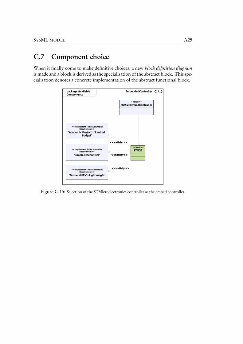
SYSML MODEL A25
C.7 Component choiceWhen it finally come to make definitive choices, a new block definition diagramis made and a block is derived as the specialisation of the abstract block. This spe-cialisation denotes a concrete implementation of the abstract functional block.
package Available
Components
EmbeddedController 1/1
<<block>>
MUAV::EmbedController
<<block>>
STM32
<<requirement,Tools::Constraint
Requirement>>
'Academic Project'::'Limited
Budget'
<<requirement,Tools::UseabilityRequirement>>
'Simple Mechanism'
<<satisfy>>
<<satisfy>>
<<requirement,Tools::ConstraintRequirement>>
'Drone MUAV'::Lightweight
<<satisfy>>
Figure C.15: Selection of the STMicroelectronics controller as the embed controller.

A26 CONTROL OF A MINI UNMANNED AERIAL VEHICULE
BIBLIOGRAPHY A27
Bibliography[1] American Systems Corporation, ARTiSAN Software Tools, BAE SYS-
TEMS, The Boeing Company, Ceira Technologies, Deere & Company,EADS Astrium GmbH, EmbeddedPlus Engineering, Eurostep GroupAB, Gentleware AG, Inc. I-Logix, International Business Machines,International Council on Systems Engineering, Israel Aircraft Indus-tries, Lockheed Martin Corporation, Mentor Graphics, Inc. Motorola,Northrop Grumman, Object Management Group, oose Innovative In-formatik GmbH, PivotPoint Technology Corporation, Raytheon Com-pany, Sparx Systems, Telelogic AB, and THALES. OMG System Model-ing Language version 1.1. Specifications, The Object Management Group,November 2008. Available from: http://www.omg.org/spec/SysML/1.1/.
[2] Richard Feynman. Rogers Commission Report on the Space Shuttle Chal-lenger Accident, appendix Personal observations on the reliability of theShuttle. Rogers Commission, June 1986. Available from: http://www.
ralentz.com/old/space/feynman-report.html.
[3] The Object Management Group. Omg sysml [online]. Available from:http://www.omgsysml.org/.
[4] The Object Management Group. Omg unified modelling language [on-line]. Available from: http://www.uml.org/.
[5] The Object Management Group. Sysml and modelica integration [on-line]. Available from: http://www.omgwiki.org/OMGSysML/doku.php?
id=sysml-modelica:sysml_and_modelica_integration.
[6] Randy Miller. Practical uml: A hands-on introduction for developers [on-line]. Available from: http://edn.embarcadero.com/article/31863.
[7] Aurélie Souletis. Mini Unmanned Aerial Vehicles Dynamic Model. Tech-nical report, Institut National des Sciences Appliquées de Toulouse, Jan-uary 2008.
[8] Tim Weilkiens. System Engineering with SysML/UML. The Morgan Kauf-mann/Object Management Group Press, 2007.
[9] Wikipédia (en) [online]. Available from: http://en.wikipedia.org/
wiki/Main_Page.
[10] Wikipédia (fr) [online]. Available from: http://fr.wikipedia.org/
wiki/Accueil.
A28 CONTROL OF A MINI UNMANNED AERIAL VEHICULE
Credits[11] MQ-9 Reaper in flight (2007), December 2007 by U.S. Air Force pho-
to/Staff Sgt. Brian Ferguson.http://en.wikipedia.org/wiki/File:MQ-9_Reaper_in_flight_
(2007).jpg
Licensed under Public Domain.
[12] Instance specification 3, April 2005 by Gubaer.http://en.wikipedia.org/wiki/File:Instance_specification_3.
png
Licensed under Public Domain.
[13] UMLUSE, October 2003 by Poor Yorick.http://en.wikipedia.org/wiki/File:UMLUSE.PNG
Licensed under GNU Free Documentation License, Version 1.2 withno Invariant Sections, no Front-Cover Texts, and no Back-Cover Texts.,http://www.gnu.org/licenses/old-licenses/fdl-1.2.txt.
[14] Flight Dynamics With Text, August 2007 by ZeroOne.http://en.wikipedia.org/wiki/File:Flight_dynamics_with_text.
png
Licensed under Creative Commons Attribution 3.0 Unported,http://creativecommons.org/licenses/by/3.0/.
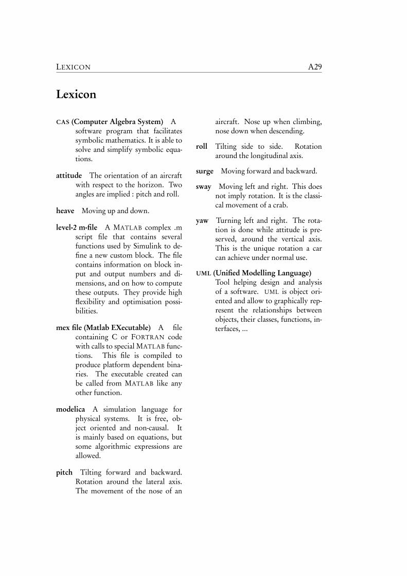
LEXICON A29
Lexicon
CAS (Computer Algebra System) Asoftware program that facilitatessymbolic mathematics. It is able tosolve and simplify symbolic equa-tions.
attitude The orientation of an aircraftwith respect to the horizon. Twoangles are implied : pitch and roll.
heave Moving up and down.
level-2 m-file A MATLAB complex .mscript file that contains severalfunctions used by Simulink to de-fine a new custom block. The filecontains information on block in-put and output numbers and di-mensions, and on how to computethese outputs. They provide highflexibility and optimisation possi-bilities.
mex file (Matlab EXecutable) A filecontaining C or FORTRAN codewith calls to special MATLAB func-tions. This file is compiled toproduce platform dependent bina-ries. The executable created canbe called from MATLAB like anyother function.
modelica A simulation language forphysical systems. It is free, ob-ject oriented and non-causal. Itis mainly based on equations, butsome algorithmic expressions areallowed.
pitch Tilting forward and backward.Rotation around the lateral axis.The movement of the nose of an
aircraft. Nose up when climbing,nose down when descending.
roll Tilting side to side. Rotationaround the longitudinal axis.
surge Moving forward and backward.
sway Moving left and right. This doesnot imply rotation. It is the classi-cal movement of a crab.
yaw Turning left and right. The rota-tion is done while attitude is pre-served, around the vertical axis.This is the unique rotation a carcan achieve under normal use.
UML (Unified Modelling Language)Tool helping design and analysisof a software. UML is object ori-ented and allow to graphically rep-resent the relationships betweenobjects, their classes, functions, in-terfaces, ...

A30 CONTROL OF A MINI UNMANNED AERIAL VEHICULE


![[Article] Unmanned aerial vehicle remotely sensed datasets, a …geodata.kr/assets/pdf/7/journal-1-1-38.pdf · generated using rotary-wing UAV(unmanned aerial vehicle) system for](https://img.pdfslide.tips/doc/110x75/5e99aef244dfab24c12e8cfc/article-unmanned-aerial-vehicle-remotely-sensed-datasets-a-generated-using-rotary-wing.jpg)