Embed Size (px)
Citation preview
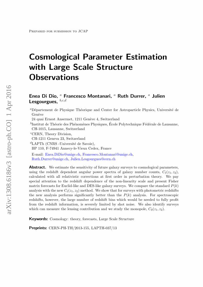
Prepared for submission to JCAP
Cosmological Parameter Estimationwith Large Scale StructureObservations
Enea Di Dio, a Francesco Montanari, a Ruth Durrer, a JulienLesgourgues, b,c,d
aDepartement de Physique Theorique and Center for Astroparticle Physics, Universite deGeneve24 quai Ernest Ansermet, 1211 Geneve 4, SwitzerlandbInstitut de Theorie des Phenomenes Physiques, Ecole Polytechnique Federale de Lausanne,CH-1015, Lausanne, SwitzerlandcCERN, Theory Division,CH-1211 Geneva 23, SwitzerlanddLAPTh (CNRS -Universite de Savoie),BP 110, F-74941 Annecy-le-Vieux Cedex, France
E-mail: [email protected], [email protected],[email protected], [email protected]
Abstract. We estimate the sensitivity of future galaxy surveys to cosmological parameters,using the redshift dependent angular power spectra of galaxy number counts, C`(z1, z2),calculated with all relativistic corrections at first order in perturbation theory. We payspecial attention to the redshift dependence of the non-linearity scale and present Fishermatrix forecasts for Euclid-like and DES-like galaxy surveys. We compare the standard P (k)analysis with the new C`(z1, z2) method. We show that for surveys with photometric redshiftsthe new analysis performs significantly better than the P (k) analysis. For spectroscopicredshifts, however, the large number of redshift bins which would be needed to fully profitfrom the redshift information, is severely limited by shot noise. We also identify surveyswhich can measure the lensing contribution and we study the monopole, C0(z1, z2).
Keywords: Cosmology: theory, forecasts, Large Scale Structure
Preprints: CERN-PH-TH/2013-155, LAPTH-037/13
arX
iv:1
308.
6186
v3 [
astr
o-ph
.CO
] 1
Apr
201
6
Contents
1 Introduction 1
2 Number counts versus the real space power spectrum 2
3 The Fisher matrix and the nonlinearity scale 53.1 Fisher matrix forecasts 53.2 The nonlinearity scale 6
4 Results 74.1 A Euclid-like catalog 74.2 A DES-like catalog 124.3 Measuring the lensing potential 154.4 The correlation function and the monopole 17
5 Conclusions 20
A The galaxy number power spectrum 21
B Basics of Fisher matrix forecasts 21
1 Introduction
Observations and analysis of the cosmic microwave background (CMB) have led to stunningadvances in observational cosmology [1, 2]. This is due on the one hand to an observationaleffort which has led to excellent data, but also to the theoretical simplicity of CMB physics.In a next (long term) step, cosmologists will try to repeat the CMB success story withobservations of large scale structures (LSS), i.e. the distribution of galaxies in the Universe.
The advantage of LSS data is the fact that it is three-dimensional, and therefore containsmuch more information than the two-dimensional CMB. The disadvantage is that the inter-pretation of the galaxy distribution is much more complicated than that of CMB anisotropies.First of all, our theoretical cosmological models predict the fluctuations of a continuous den-sity field, which we have to relate to the discrete galaxy distribution. Furthermore, on scalessmaller than 30h−1Mpc, matter density fluctuations become large and linear perturbationtheory is not sufficient to compute them. On these scales, in principle, we rely on costlyN-body simulations.
In an accompanying paper [3] we describe a code, CLASSgal, which calculates galaxynumber counts, ∆(n, z), as functions of direction n and observed redshift z in linear per-turbation theory. In this code all the relativistic effects due to peculiar motion, lensing,integrated Sachs Wolfe effect (ISW) and other effects of metric perturbations as describedin [4, 5] are fully taken into account. Even if a realistic treatment of the problem of biasingmentioned above is still missing, the number counts have the advantage that they are directlyobservable as opposed to the power spectrum of fluctuations in real space which depends oncosmological parameters. The problem how the galaxy distribution, number counts and dis-tance measurements are affected by the propagation of light in a perturbed geometry hasalso been investigated in other works; see, e.g. [6–11].
– 1 –
In this paper we use CLASSgal to make forecasts for the ability to measure cosmologicalparameters from Euclid-like and DES-like galaxy surveys. This also helps to determine opti-mal observational specifications for such a survey. The main goal of the paper is to comparethe traditional P (k) analysis of large scale structure with the new C`(z1, z2) method. Todo this we shall study and compare the figure of merit (FoM) for selected pairs of parame-ters. As our goal is not a determination of the cosmological parameters but a comparisonof methods, we shall not use constraints on the parameters from the Planck results or othersurveys. We just use the Planck best fit values as the fiducial values for our Fisher matrixanalysis. We mainly want to analyze the sensitivity of the results to redshift binning, and tothe inclusion of cross correlations, i.e., correlations at different redshifts. We shall also studythe signal-to-noise of the different contributions to C`(z1, z2) in order to decide whether theyare measurable with future surveys.
In the next section we exemplify how the same number counts lead to different 3D powerspectra when different cosmological parameters are employed. In Section 3 we use the Fishermatrix technique to estimate cosmological parameters from the number count spectrum. Wepay special attention on the non-linearity scale which enters in a non-trivial way in the Fishermatrix. We then determine the precision with which we can estimate cosmological parametersfor different choices of redshift bins and angular resolution. In Section 4 we discuss our resultsand put them into perspective. In Section 5 we conclude. Some details on the Fisher matrixtechnique and the basic formula for the number counts are given in the appendix.
2 Number counts versus the real space power spectrum
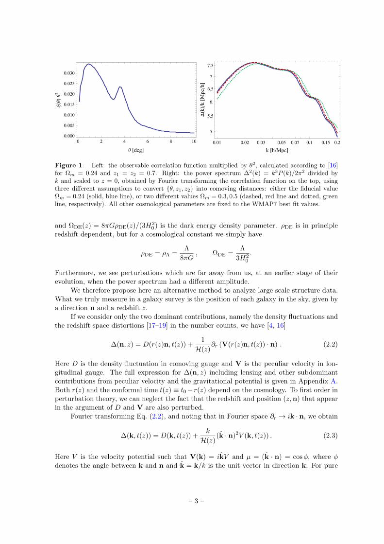
In this section we illustrate explicitly that the 3D power spectrum is not directly observable.This fact is not new, but it seems not to prevent the community from using the powerspectrum which itself depends on cosmological parameters to estimate the latter. This isthen usually taken into account by a recursive method: one chooses a set of cosmologicalparameters (usually the best fit parameters from CMB observations), determines the powerspectrum under the assumption that this set correctly describes the background cosmology,and then estimates a new set of cosmological parameters. This process is repeated withthe new parameters until convergence is reached, see [12–15] and others. It is certainlypossible to find the best fit parameters in this way, but a correct determination of the errorsis more complicated, since not only the power spectrum but also its argument k dependson cosmological parameters. In Fig. 1 we show what happens when a measured correlationfunction is converted into a power spectrum using the wrong cosmological parameters.
The advantage of using the power spectrum is that different Fourier modes are inprinciple independent. Therefore, errors on the power spectrum are independent. Fur-thermore, for small redshifts, z 1, the parameter dependence of the distance is simplyr(z) ' H−1
0 z, z 1, where H0 denotes the Hubble constant. This is usually absorbed bymeasuring distances in units of h−1Mpc. However, for large redshifts the relation becomesmore complicated,
r(z) =
∫ z
0
dz′
H(z′), (2.1)
where H(z) = H0
(Ωm(1 + z)3 + ΩK(1 + z)2 + ΩDE(z)
)1/2, Ωm = 8πGρm/(3H
20 ) denotes
the present matter density parameter, ΩK = −K/H20 is the present curvature parameter,
– 2 –
0 2 4 6 8 10
0.000
0.005
0.010
0.015
0.020
0.025
0.030
Θ @degD
ΞHΘL
Θ2
0.01 0.02 0.03 0.05 0.07 0.1 0.15 0.2
5.
5.5
6.
6.5
7.
7.5
k @hMpcD
DHkL
k@M
pch
D
Figure 1. Left: the observable correlation function multiplied by θ2, calculated according to [16]for Ωm = 0.24 and z1 = z2 = 0.7. Right: the power spectrum ∆2(k) = k3P (k)/2π2 divided byk and scaled to z = 0, obtained by Fourier transforming the correlation function on the top, usingthree different assumptions to convert θ, z1, z2 into comoving distances: either the fiducial valueΩm = 0.24 (solid, blue line), or two different values Ωm = 0.3, 0.5 (dashed, red line and dotted, greenline, respectively). All other cosmological parameters are fixed to the WMAP7 best fit values.
and ΩDE(z) = 8πGρDE(z)/(3H20 ) is the dark energy density parameter. ρDE is in principle
redshift dependent, but for a cosmological constant we simply have
ρDE = ρΛ =Λ
8πG, ΩDE =
Λ
3H20
.
Furthermore, we see perturbations which are far away from us, at an earlier stage of theirevolution, when the power spectrum had a different amplitude.
We therefore propose here an alternative method to analyze large scale structure data.What we truly measure in a galaxy survey is the position of each galaxy in the sky, given bya direction n and a redshift z.
If we consider only the two dominant contributions, namely the density fluctuations andthe redshift space distortions [17–19] in the number counts, we have [4, 16]
∆(n, z) = D(r(z)n, t(z)) +1
H(z)∂r (V(r(z)n, t(z)) · n) . (2.2)
Here D is the density fluctuation in comoving gauge and V is the peculiar velocity in lon-gitudinal gauge. The full expression for ∆(n, z) including lensing and other subdominantcontributions from peculiar velocity and the gravitational potential is given in Appendix A.Both r(z) and the conformal time t(z) ≡ t0−r(z) depend on the cosmology. To first order inperturbation theory, we can neglect the fact that the redshift and position (z,n) that appearin the argument of D and V are also perturbed.
Fourier transforming Eq. (2.2), and noting that in Fourier space ∂r → ik · n, we obtain
∆(k, t(z)) = D(k, t(z)) +k
H(z)(k · n)2V (k, t(z)) . (2.3)
Here V is the velocity potential such that V(k) = ikV and µ = (k · n) = cosφ, where φdenotes the angle between k and n and k = k/k is the unit vector in direction k. For pure
– 3 –
matter perturbations, the time dependence of D is independent of wave number such that
D(k, t(z)) = G(z)D(k, t0) ,
where G(z) describes the growth of linear matter perturbations. For pure matter perturba-tions, the continuity equation [1] implies
k
H(z)V (k, t(z)) = f(z)D(k, t(z)) , where f(z) =
1 + z
G
dG
dz=
d logG
d log(1 + z)(2.4)
is the growth factor. Inserting this in Eq. (2.3), we obtain the following relation for a fixedangle between k and the direction of observation, and for a fixed redshift z:
P∆(k, z) = G2(z)(1 + µ2f(z)
)2PD(k) . (2.5)
If we have only one redshift bin at our disposition, the factor G2 is in principle degeneratewith a constant bias and the overall amplitude of PD(k). A more general expression fordifferent redshifts and directions can be found in Ref. [16].
Measuring the redshift space distortions that are responsible for the angular dependenceof P∆ allows in principle to measure the growth factor, f(z). Furthermore, assuming thatdensity fluctuations relate to the galaxy density by some bias factor b(z, k), while the velocitiesare not biased, the first term in Eq. 2.5 becomes proportional to (b(z, k)G(z))2 while thesecond term behaves like G(z)f(z). This feature allows in principle to reconstruct the biasfunction b(z, k). It is an interesting question whether this bias can be measured better withour angular analysis or with the standard power spectrum analysis. However, since it isprobably not strongly dependent on cosmological parameters, its reconstruction with thepower spectrum method seems quite adequate and probably simpler. In the remainder of thepresent work we shall therefore not address the interesting question of bias, see e.g. [20, 21].
However, in the above approximation, both relativistic effects which can be relevant onlarge scales as well as a possible clustering of dark energy are neglected. On top of that, thematter power spectrum in Fourier space is not directly observable. Several steps (like therelation between Fourier wave numbers and galaxy positions) can only be performed underthe assumption of a given background cosmology. What we truly measure is a correlationfunction ξ(θ, z, z′), for galaxies at redshifts z and z′ in directions n and n′, where θ is the anglebetween the two directions, n · n′ = cos θ. The correlation function analysis of cosmologicalsurveys has a long tradition. But the correlation function has usually been considered asa function of the distance r between galaxies which of course has the same problem as itsFourier transform, the power spectrum: it depends on the cosmological parameters used todetermine r.
For these reasons, we work instead directly with the correlation function and powerspectra in angular and redshift space. They are related by
ξ(θ, z, z′) ≡ 〈∆(n, z)∆(n′, z′)〉 =1
4π
∞∑`=0
(2`+ 1)C`(z, z′)P`(cos θ) , (2.6)
where P`(x) is the Legendre polynomial of degree `. The power spectra C`(z, z′) can also be
defined via
∆(n, z) =∑`m
a`m(z)Y`m(n) , C`(z, z′) = 〈a`m(z)a∗`m(z′)〉 , (2.7)
– 4 –
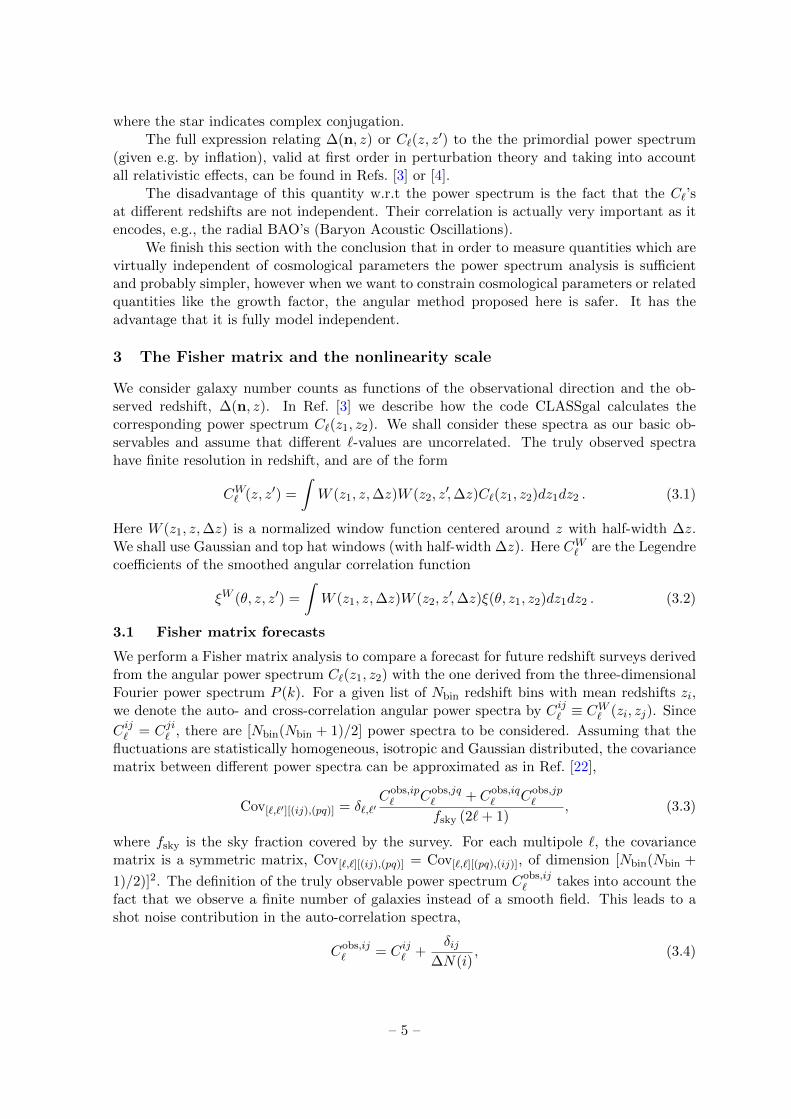
where the star indicates complex conjugation.The full expression relating ∆(n, z) or C`(z, z
′) to the the primordial power spectrum(given e.g. by inflation), valid at first order in perturbation theory and taking into accountall relativistic effects, can be found in Refs. [3] or [4].
The disadvantage of this quantity w.r.t the power spectrum is the fact that the C`’sat different redshifts are not independent. Their correlation is actually very important as itencodes, e.g., the radial BAO’s (Baryon Acoustic Oscillations).
We finish this section with the conclusion that in order to measure quantities which arevirtually independent of cosmological parameters the power spectrum analysis is sufficientand probably simpler, however when we want to constrain cosmological parameters or relatedquantities like the growth factor, the angular method proposed here is safer. It has theadvantage that it is fully model independent.
3 The Fisher matrix and the nonlinearity scale
We consider galaxy number counts as functions of the observational direction and the ob-served redshift, ∆(n, z). In Ref. [3] we describe how the code CLASSgal calculates thecorresponding power spectrum C`(z1, z2). We shall consider these spectra as our basic ob-servables and assume that different `-values are uncorrelated. The truly observed spectrahave finite resolution in redshift, and are of the form
CW` (z, z′) =
∫W (z1, z,∆z)W (z2, z
′,∆z)C`(z1, z2)dz1dz2 . (3.1)
Here W (z1, z,∆z) is a normalized window function centered around z with half-width ∆z.We shall use Gaussian and top hat windows (with half-width ∆z). Here CW` are the Legendrecoefficients of the smoothed angular correlation function
ξW (θ, z, z′) =
∫W (z1, z,∆z)W (z2, z
′,∆z)ξ(θ, z1, z2)dz1dz2 . (3.2)
3.1 Fisher matrix forecasts
We perform a Fisher matrix analysis to compare a forecast for future redshift surveys derivedfrom the angular power spectrum C`(z1, z2) with the one derived from the three-dimensionalFourier power spectrum P (k). For a given list of Nbin redshift bins with mean redshifts zi,we denote the auto- and cross-correlation angular power spectra by Cij` ≡ C
W` (zi, zj). Since
Cij` = Cji` , there are [Nbin(Nbin + 1)/2] power spectra to be considered. Assuming that thefluctuations are statistically homogeneous, isotropic and Gaussian distributed, the covariancematrix between different power spectra can be approximated as in Ref. [22],
Cov[`,`′][(ij),(pq)] = δ`,`′Cobs,ip` Cobs,jq
` + Cobs,iq` Cobs,jp
`
fsky (2`+ 1), (3.3)
where fsky is the sky fraction covered by the survey. For each multipole `, the covariancematrix is a symmetric matrix, Cov[`,`][(ij),(pq)] = Cov[`,`][(pq),(ij)], of dimension [Nbin(Nbin +
1)/2)]2. The definition of the truly observable power spectrum Cobs,ij` takes into account the
fact that we observe a finite number of galaxies instead of a smooth field. This leads to ashot noise contribution in the auto-correlation spectra,
Cobs,ij` = Cij` +
δij∆N(i)
, (3.4)
– 5 –
where ∆N(i) is the number of galaxies per steradian in the i-th redshift bin. In principlealso instrumental noise has to be added, but we neglect it here, assuming that it is smallerthan the shot noise. More details about the Fisher matrix and the definition of ’figure ofmerit’ (FoM) are given in Appendix B.
3.2 The nonlinearity scale
Our code CLASSgal uses linear perturbation theory, which is valid only for small densityfluctuations, D = δρm/ρm 1. However, on scales roughly of the order of λ . 30h−1Mpc,the observed density fluctuations are of order unity and larger at late times. In order tocompute their evolution, we have to resort to Newtonian N-body simulations, which is beyondthe scope of this work. Also, on non-linear scales, the Gaussian approximation used inour expression for likelihoods and Fisher matrices becomes incorrect. Hence, there exists amaximal wavenumber kmax and a minimal comoving wavelength,
λmin =2π
kmax
beyond which we cannot trust our calculations. There are more involved procedures to dealwith non-linearities instead of using a simple cutoff, see e.g. [23]. However, in this work wefollow the conservative approach of a cutoff.
For a given power spectrum Cij` this nonlinear cutoff translates into an `-dependent andredshift-dependent distance which can be approximated as follows. The harmonic mode `primarily measures fluctuations on an angular scale1 θ(`) ∼ 2π/`. Let us consider two binswith mean redshifts zi ≤ zj and half-widths ∆zi and ∆zj . At a mean redshift z = (zi+ zj)/2the scale θ(`) corresponds to a comoving distance r` = r(z)θ(`), where r(z) denotes thecomoving distance to z. Let us define the “bin separation” δzij = zinf
j − zsupi , where zinf
j =zj −∆zj and zsup
i = zi + ∆zi. Hence δzij is positive for well-separated bins, and negative foroverlapping bins (or for the case of an auto-correlation spectrum with i = j)2.
When δzij < 0, excluding non-linear scales simply amounts in considering correlationsonly for distances r` > λmin. When δzij > 0, the situation is different. The comoving radialdistance corresponding to the bin separation δzij is rz = δzij H
−1(z). If rz > λmin, wecan consider correlations on arbitrarily small angular scales without ever reaching non-linearwavelengths (in that case, the limiting angular scale is set by the angular resolution of theexperiment). Finally, in the intermediate case such that 0 < δzijH
−1(z) < λmin, the smallest
wavelength probed by a given angular scale is given by√r2` + r2
z . In summary, the condition
1Here we refer to the angular scale separating two consecutive maxima in a harmonic expansion, and notto the scale separating consecutive maxima and minima, given by π/`. Since we want to relate angular scalesto Fourier modes, and Fourier wavelengths also refer to the distance between two consecutive maxima, therelation θ(`) = 2π/` is the relevant one in this context.
2 In the case of a spectroscopic survey, we will use top-hat window functions. In this case there is noambiguity in the definition of δzij , since (zsup
i , zinfj ) are given by the sharp edges of the top-hats. In the
case of a photometric survey, we will work with Gaussian window functions. Then (zsupi , zinf
j ) can only bedefined as the redshifts standing at an arbitrary number of standard deviations away from the mean redshifts(zi, zj). In the following, the standard deviation in the i-th redshift bin is denoted ∆zi, and we decided toshow results for two different definitions of the “bin separation”, corresponding either to 2σ distances, withzinfj = zj − 2∆zj and zsup
i = zi + 2∆zi, or to 3σ distances, with zinfj = zj − 3∆zj and zsup
i = zi + 3∆zi.
– 6 –
to be fulfilled by a given angular scale θ(`) and by the corresponding multipole ` is
λmin ≤
2π` r(z) if δzij ≤ 0 ,√(
δzijH(z)
)2+(
2π` r(z)
)2if 0 ≤ δzij ≤ H(z)λmin .
(3.5)
The highest multipole fulfilling these inequalities is
`ijmax =
2πr(z)/λmin if δzij ≤ 0 ,
2πr(z)√λ2
min−(δzijH(z)
)2if 0 <
δzijH(z) < λmin ,
∞ otherwise.
(3.6)
In the last case, the cut-off is given by the experimental angular resolution, `ijmax = 2π/θexp.
Only multipoles Cij` which satisfy the condition ` ≤ `ijmax are taken into account in ouranalysis. In the covariance matrix, for the spectra of redshift bins (ij) and (pq), we cut offthe sum over multipoles in the Fisher matrix, Eq. (B.1) at
`max = min(`ijmax, `pqmax) . (3.7)
The nonlinearity scale is fixed by the smallest redshift difference appearing in the two pairs(ij), (pq). This condition ensures that nonlinear scales do not contribute to the derivatives inthe Fisher matrix, Eq. (B.1). This is an important limitation because nonlinear scales containa large amount of information. Clearly, it will be necessary to overcome this limitation atleast partially to profit maximally from future surveys. Notice that with `max as in Eq. (3.7)the the Fisher matrix can still involve non-linear contributions, but these are confined to theinverse of the covariance matrix (3.3) where also the spectra (iq), (jp), (ip) and (jq) appear.Of course, we need to use values for the cosmological parameters to determine r(z) and H(z)in (3.5), but since this condition is approximate, this does not significantly compromise ourresults.
4 Results
We now present Fisher matrix forecasts for several different types of surveys. In the errorbudget we only take into account sample variance, shot noise and photometric redshift (photo-z) uncertainties. In this sense, our results are not very realistic: the true analysis, containingalso instrumental noise, is certainly more complicated. Nevertheless, we believe that thisexercise is useful for the comparison of different methods and different surveys.
In what follows we refer to the P (k) analysis as the 3D case, and to the C` analysis asthe 2D case. We assume a fiducial cosmology described by the minimal (flat) ΛCDM model,neglecting neutrino masses. We study the dependence on the following set of cosmologicalparameters: (ωb ≡ Ωbh
2, ωCDM ≡ ΩCDMh2, H0, As, ns), which denote the baryon and
CDM density parameters, the Hubble parameter, the amplitude of scalar perturbation andthe scalar spectral index, respectively. We set the curvature K = 0.
4.1 A Euclid-like catalog
In this section we perform a Fisher matrix analysis for an Euclid-like catalog. We comparethe galaxy surveys with spectral and photometric redshifts. We show the dependence of the
– 7 –
0.8 1.0 1.2 1.4 1.6 1.8 2.0
103
2 ´ 103
3 ´ 103
4 ´ 103
z
dNd
z
0.8 1.0 1.2 1.4 1.6 1.8 2.0
105
2 ´ 105
3 ´ 105
4 ´ 105
z
dNd
z
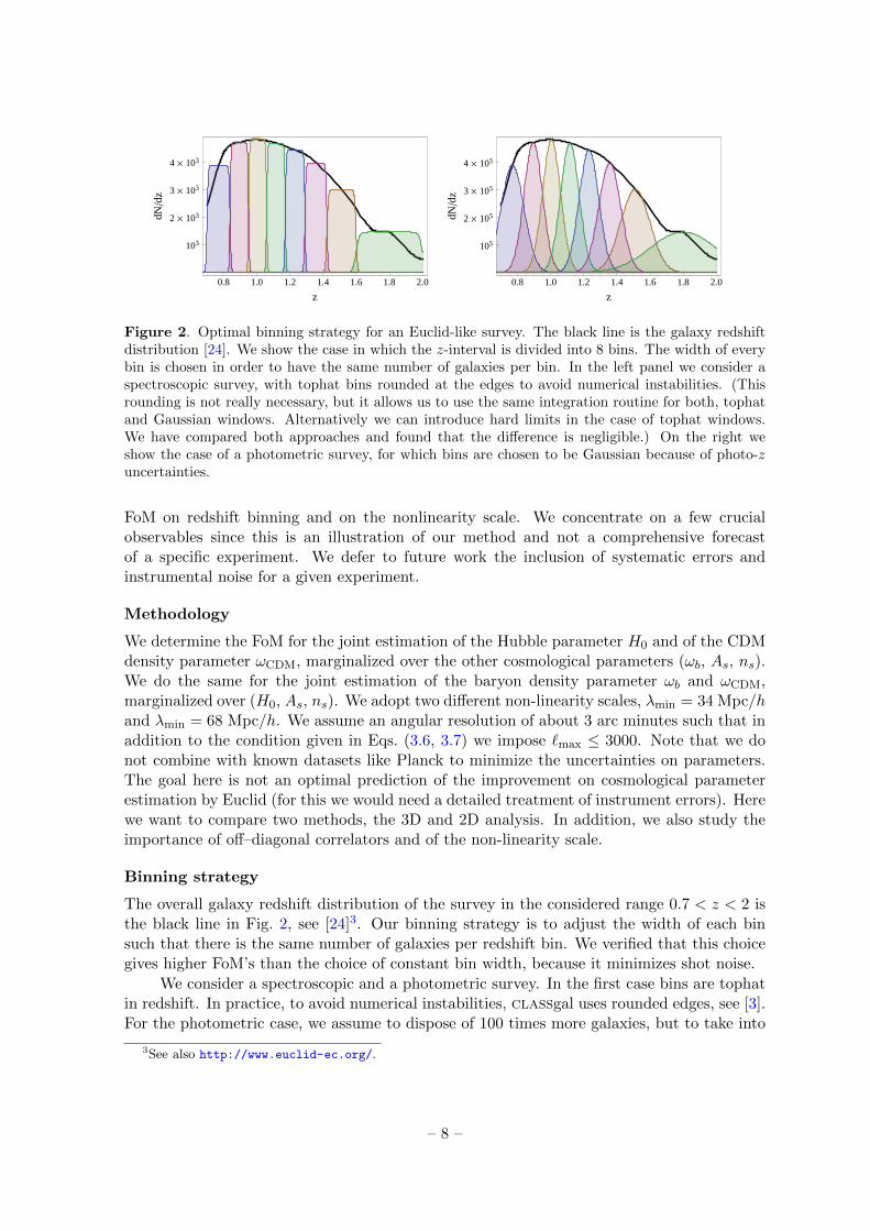
Figure 2. Optimal binning strategy for an Euclid-like survey. The black line is the galaxy redshiftdistribution [24]. We show the case in which the z-interval is divided into 8 bins. The width of everybin is chosen in order to have the same number of galaxies per bin. In the left panel we consider aspectroscopic survey, with tophat bins rounded at the edges to avoid numerical instabilities. (Thisrounding is not really necessary, but it allows us to use the same integration routine for both, tophatand Gaussian windows. Alternatively we can introduce hard limits in the case of tophat windows.We have compared both approaches and found that the difference is negligible.) On the right weshow the case of a photometric survey, for which bins are chosen to be Gaussian because of photo-zuncertainties.
FoM on redshift binning and on the nonlinearity scale. We concentrate on a few crucialobservables since this is an illustration of our method and not a comprehensive forecastof a specific experiment. We defer to future work the inclusion of systematic errors andinstrumental noise for a given experiment.
Methodology
We determine the FoM for the joint estimation of the Hubble parameter H0 and of the CDMdensity parameter ωCDM, marginalized over the other cosmological parameters (ωb, As, ns).We do the same for the joint estimation of the baryon density parameter ωb and ωCDM,marginalized over (H0, As, ns). We adopt two different non-linearity scales, λmin = 34 Mpc/hand λmin = 68 Mpc/h. We assume an angular resolution of about 3 arc minutes such that inaddition to the condition given in Eqs. (3.6, 3.7) we impose `max ≤ 3000. Note that we donot combine with known datasets like Planck to minimize the uncertainties on parameters.The goal here is not an optimal prediction of the improvement on cosmological parameterestimation by Euclid (for this we would need a detailed treatment of instrument errors). Herewe want to compare two methods, the 3D and 2D analysis. In addition, we also study theimportance of off–diagonal correlators and of the non-linearity scale.
Binning strategy
The overall galaxy redshift distribution of the survey in the considered range 0.7 < z < 2 isthe black line in Fig. 2, see [24]3. Our binning strategy is to adjust the width of each binsuch that there is the same number of galaxies per redshift bin. We verified that this choicegives higher FoM’s than the choice of constant bin width, because it minimizes shot noise.
We consider a spectroscopic and a photometric survey. In the first case bins are tophatin redshift. In practice, to avoid numerical instabilities, classgal uses rounded edges, see [3].For the photometric case, we assume to dispose of 100 times more galaxies, but to take into
3See also http://www.euclid-ec.org/.
– 8 –
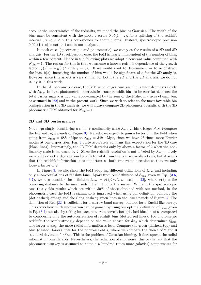
account the uncertainties of the redshifts, we model the bins as Gaussian. The width of thebins must be consistent with the photo-z errors 0.05(1 + z), for a splitting of the redshiftinterval 0.7 < z < 2 this corresponds to about 6 bins. Instead, spectroscopic precision0.001(1 + z) is not an issue in our analysis.
In both cases (spectroscopic and photometric), we compare the results of a 2D and 3Danalysis. For the 3D spectroscopic case, the FoM is nearly independent of the number of bins,within a few percent. Hence in the following plots we adopt a constant value computed withNbin = 1. The reason for this is that we assume a known redshift dependence of the growthfactor, f(z) = ΩM (z)γ with γ = 0.6. If we would want to determine γ or to reconstructthe bias, b(z), increasing the number of bins would be significant also for the 3D analysis.However, since this aspect is very similar for both, the 2D and the 3D analysis, we do notstudy it in this work.
In the 3D photometric case, the FoM is no longer constant, but rather decreases slowlywith Nbin. In fact, photometric uncertainties cause redshift bins to be correlated, hence thetotal Fisher matrix is not well approximated by the sum of the Fisher matrices of each bin,as assumed in [22] and in the present work. Since we wish to refer to the most favorable binconfiguration in the 3D analysis, we will always compare 2D photometric results with the 3Dphotometric FoM obtained for Nbin = 1.
2D and 3D performances
Not surprisingly, considering a smaller nonlinearity scale λmin yields a larger FoM (comparethe left and right panels of Figure 3). Naively, we expect to gain a factor 8 in the FoM whengoing from λmin = 68h−1Mpc to λmin = 34h−1Mpc, since we have 23 times more Fouriermodes at our disposition. Fig. 3 quite accurately confirms this expectation for the 3D case(black lines). Interestingly, the 2D FoM degrades only by about a factor of 2 when the non-linearity scale is increased by 2. Since the redshift resolution is not affected by λmin, naivelywe would expect a degradation by a factor of 4 from the transverse directions, but it seemsthat the redshift information is as important as both transverse direction so that we onlyloose a factor of 2.
In Figure 3, we also show the FoM adopting different definitions of `max and includingonly auto-correlations of redshift bins. Apart from our definition of `max given in Eqs. (3.6,3.7), we also consider the definition `max = r(z)2π/λmin used in [22], where r(z) is thecomoving distance to the mean redshift z = 1.35 of the survey. While in the spectroscopiccase this yields results which are within 30% of those obtained with our method, in thephotometric case the FoM is significantly improved when using our definition, compare the(dot-dashed) orange and the (long dashed) green lines in the lower panels of Figure 3. Thedefinition of Ref. [22] is sufficient for a narrow band survey, but not for a Euclid-like survey.This shows how much information can be gained by using our optimal definition of `max givenin Eq. (3.7) but also by taking into account cross-correlations (dashed blue lines) as comparedto considering only the auto-correlation of redshift bins (dotted red lines). For photometricredshifts the result strongly depends on the value chosen for δzij which determines `ijmax.The larger is δzij , the more radial information is lost. Compare the green (dashed, top) andblue (dashed, lower) lines for the photo-z FoM’s, where we compare the choice of 2 and 3standard deviation for δzij . This is the problem of Gaussian binning. It does spread the radialinformation considerably. Nevertheless, the reduction of shot noise (due to the fact that thephotometric survey is assumed to contain a hundred times more galaxies) compensates for
– 9 –
λmin = 34h−1Mpc λmin = 68h−1Mpc
Spectroscopic
4 10 15 20 30
5
10
50
100
500
NBins
FoM
ΩC
DM
-H
0
Spectroscopic
4 10 15 20 30
5
10
50
100
500
NBins
FoM
ΩC
DM
-H
0
Photo-z
4 5 6 7 8
5
10
50
100
500
NBins
FoM
ΩC
DM
-H
0
Photo-z
4 5 6 7 8
5
10
50
100
500
NBins
FoM
ΩC
DM
-H
0
Figure 3. FoM for an Euclid-like survey for the non-linearity scales 34 Mpc/h, left panels, and68 Mpc/h, right panels. Top panels refer to spectroscopic redshifts, bottom panels to photometricones. For the 2D FoM we consider a cut at `max values defined in Eq. (3.7) (dashed blue), and alsothe case in which cross-correlations of bins are neglected (dotted red). For the photometric survey,we plot the result derived from two different definitions of the bin separation (and hence of `max),defining (zsupi , zinfj ) at either 2- (green) or 3-σ (blue), see Footnote 2. For this case we also plot theFoM for the `max determination of Ref. [22] (dot-dashed orange). The solid black line shows the valueof the 3D FoM for Nbin = 1 and σz = 0.05(1 + z) in the photometric case. The shadowed regionexceeds this z resolution.
this, and leads to a better FoM from photometric surveys in the 2D analysis. However, inthe spectroscopic case we could still increase the number of bins.
Interestingly, with the more conservative value of the non-linearity scale λmin = 68 Mpc/h(right hand panels of Fig. 3), the difference between the full analysis (blue, dashed) and theone involving only auto-correlations (red, dotted) becomes very significant also for spec-troscopic surveys. When considering only auto-correlations, the spectroscopic FoM reachessaturation at 16 bins. One reason for this is that shot noise affects auto-correlations morestrongly than cross-correlations. But even neglecting shot noise, we still observe this satura-tion. We just cannot gain more information from the auto-correlations alone by increasingthe number of bins, i.e. by a finer sampling of transverse correlations.
Comparing the spectroscopic with the photometric survey and sticking to the 2D analy-sis, we find that the photometric specifications yield a larger FoM. This is not surprising, sincethe latter case contains 100 times more galaxies than the spectroscopic survey, for which shotnoise is correspondingly 100 times larger. Also, the FoM for the 2D analysis mainly comesfrom cross correlations. This is why different choices of δzij affect the final result so much.
The photometric FoM from the 3D analysis, however, is lower than the one from thespectroscopic survey. In the 3D case, the redshift uncertainties translate into uncertainties
– 10 –
in the wavenumber k which are more relevant than the reduction of shot noise.
When the number of bins is large enough, our 2D analysis yields a better FoM than thestandard P (k) analysis. For the photometric survey this is achieved already at Nbin = 4− 6while for the spectroscopic survey probably about 120 bins would be needed.
At some maximal number of bins the number of galaxies per bin becomes too smalland shot noise starts to dominate. At this point nothing more can be gained from increasingthe number of bins. However, since for slimmer redshift bins not only the shot noise butalso the signal increases, see [3] for details, the optimal number of bins is larger than a naiveestimate. In Ref. [3] it is shown that the shot noise, which behaves like `(` + 1)/2π (in aplot of `(`+ 1)C`/2π), becomes of the order of the signal at somewhat smaller ` for slimmerredshift bins. Again, due to the increase of the signal this dependence is rather weak downto a redshift width of ∆z = 0.0065. For redshift slices with ∆z < 0.005, the signal doesnot increase anymore while the shot noise still does. For a DES-like survey, this maximal
number of bins is about N(DES)max ∼ 50, while for a Euclid-like survey it is of the order of
N(Euclid)max ∼ 200.
When using redshift bins which are significantly thicker than the redshift resolution ofthe survey, the 3D analysis, in principle, has an advantage since it makes use of the full redshiftresolution in determining distances of galaxies, while in the 2D analysis we do not distinguishredshifts of galaxies in the same bin. A redshift bin width of the order of the nonlinearityscale beyond which the power spectrum is not reliable, given by r(z,∆z) ∼ 2∆z/H(z) ' λmin
is the minimum needed to recover the 3D FoM for spectroscopic surveys.
However, for spectroscopic surveys we can in principle allow for very slim bins with athickness significantly smaller than the nonlinearity scale, and the maximal number of usefulbins is decided by the shot noise. Comparing the Cii` with Cjj` , e.g., of neighboring bins still
contains some information, e.g., on the growth factor, even if `ijmax ∼ `iimax for small |i − j|.In simpler terms, the fact that our analysis effectively splits transversal information comingfrom a given redshift and radial information from Cij` with large `, makes it in principleadvantageous over the P (k) analysis. It becomes clear from Fig. 3 (see also Fig. 7 below)that we need to use sufficiently many bins and our definition of `ijmax to fully profit from thisadvantage.
The numerical effort of a Markov Chain Monte Carlo analysis of real data scales roughlylike N2
bin. Running a full chain of, say 105 points in parameter space requires the calculationof about 105N2
bin/2 spectra with class. (For comparison, a CMB chain requires ‘only’ 4×10⁵
spectra).
Note also, that the advantage of the 2D method is relevant only when we want toestimate cosmological parameters. If the cosmology is assumed to be known and we want,e.g., to reconstruct the bias of galaxies w.r.t. matter density fluctuations, both methods areequivalent. But then, the redshift dependence also of P (k) has to be studied and both powerspectra, P (k, µ, z) and C`(z, z
′) are functions of three variables.
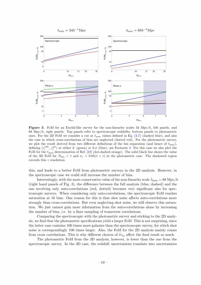
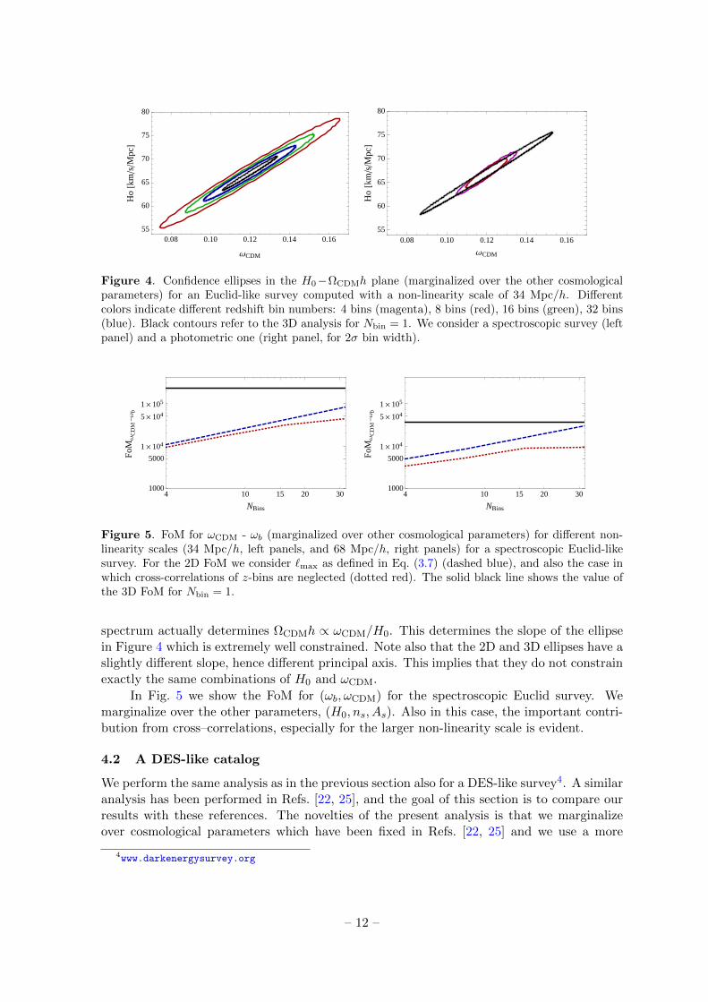
In Figure 4 we plot, as one of several possible examples, the confidence ellipses in theH0−ωCDM plane (marginalized over the other cosmological parameters) for an Euclid-likesurvey computed with a nonlinearity scale of 34 Mpc/h for different redshift bins. We donot assume any prior knowledge e.g. from Planck. Therefore again, this is not a competitiveparameter estimation but only a comparison of methods. We also show the dependence ofthe result on the number of bins. The strong degeneracy between H0 and ωCDM comes fromthe fact that ωCDM is mainly determined by the break in the power spectrum at the equalityscale keq which of course also depends on H0. As is well known, the break in the power
– 11 –
0.08 0.10 0.12 0.14 0.1655
60
65
70
75
80
ΩCDM
Ho
@km
sM
pcD
0.08 0.10 0.12 0.14 0.1655
60
65
70
75
80
ΩCDM
Ho
@km
sM
pcD
Figure 4. Confidence ellipses in the H0−ΩCDMh plane (marginalized over the other cosmologicalparameters) for an Euclid-like survey computed with a non-linearity scale of 34 Mpc/h. Differentcolors indicate different redshift bin numbers: 4 bins (magenta), 8 bins (red), 16 bins (green), 32 bins(blue). Black contours refer to the 3D analysis for Nbin = 1. We consider a spectroscopic survey (leftpanel) and a photometric one (right panel, for 2σ bin width).
4 10 15 20 301000
5000
1 ´ 104
5 ´ 104
1 ´ 105
NBins
FoM
ΩC
DM
-Ω
b
4 10 15 20 301000
5000
1 ´ 104
5 ´ 104
1 ´ 105
NBins
FoM
ΩC
DM
-Ω
b
Figure 5. FoM for ωCDM - ωb (marginalized over other cosmological parameters) for different non-linearity scales (34 Mpc/h, left panels, and 68 Mpc/h, right panels) for a spectroscopic Euclid-likesurvey. For the 2D FoM we consider `max as defined in Eq. (3.7) (dashed blue), and also the case inwhich cross-correlations of z-bins are neglected (dotted red). The solid black line shows the value ofthe 3D FoM for Nbin = 1.
spectrum actually determines ΩCDMh ∝ ωCDM/H0. This determines the slope of the ellipsein Figure 4 which is extremely well constrained. Note also that the 2D and 3D ellipses have aslightly different slope, hence different principal axis. This implies that they do not constrainexactly the same combinations of H0 and ωCDM.
In Fig. 5 we show the FoM for (ωb, ωCDM) for the spectroscopic Euclid survey. Wemarginalize over the other parameters, (H0, ns, As). Also in this case, the important contri-bution from cross–correlations, especially for the larger non-linearity scale is evident.
4.2 A DES-like catalog
We perform the same analysis as in the previous section also for a DES-like survey4. A similaranalysis has been performed in Refs. [22, 25], and the goal of this section is to compare ourresults with these references. The novelties of the present analysis is that we marginalizeover cosmological parameters which have been fixed in Refs. [22, 25] and we use a more
4www.darkenergysurvey.org
– 12 –
4 10 15 20 30
0.5
1.0
5.0
10.0
50.0
NBins
FoM
ΩC
DM
-H
0
4 10 15 20 30
0.5
1.0
5.0
10.0
50.0
NBins
FoM
ΩC
DM
-H
0
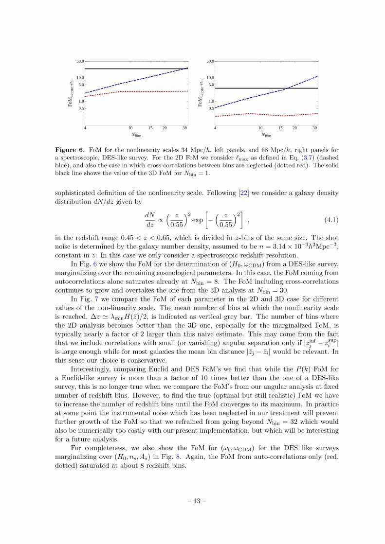
Figure 6. FoM for the nonlinearity scales 34 Mpc/h, left panels, and 68 Mpc/h, right panels fora spectroscopic, DES-like survey. For the 2D FoM we consider `max as defined in Eq. (3.7) (dashedblue), and also the case in which cross-correlations between bins are neglected (dotted red). The solidblack line shows the value of the 3D FoM for Nbin = 1.
sophisticated definition of the nonlinearity scale. Following [22] we consider a galaxy densitydistribution dN/dz given by
dN
dz∝( z
0.55
)2exp
[−( z
0.55
)2], (4.1)
in the redshift range 0.45 < z < 0.65, which is divided in z-bins of the same size. The shotnoise is determined by the galaxy number density, assumed to be n = 3.14× 10⁻³h3Mpc−3,constant in z. In this case we only consider a spectroscopic redshift resolution.
In Fig. 6 we show the FoM for the determination of (H0, ωCDM) from a DES-like survey,marginalizing over the remaining cosmological parameters. In this case, the FoM coming fromautocorrelations alone saturates already at Nbin = 8. The FoM including cross-correlationscontinues to grow and overtakes the one from the 3D analysis at Nbin = 30.
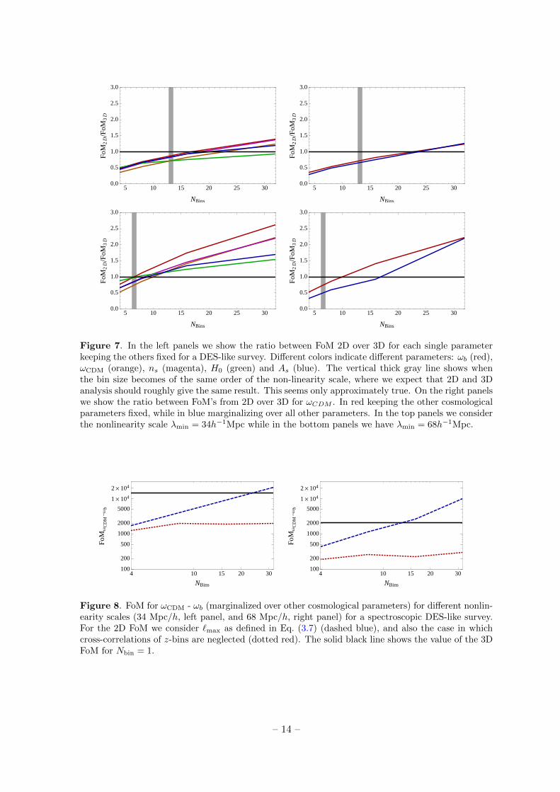
In Fig. 7 we compare the FoM of each parameter in the 2D and 3D case for differentvalues of the non-linearity scale. The mean number of bins at which the nonlinearity scaleis reached, ∆z ' λminH(z)/2, is indicated as vertical grey bar. The number of bins wherethe 2D analysis becomes better than the 3D one, especially for the marginalized FoM, istypically nearly a factor of 2 larger than this naive estimate. This may come from the factthat we include correlations with small (or vanishing) angular separation only if |zinf
j − zsupi |
is large enough while for most galaxies the mean bin distance |zj − zi| would be relevant. Inthis sense our choice is conservative.
Interestingly, comparing Euclid and DES FoM’s we find that while the P (k) FoM fora Euclid-like survey is more than a factor of 10 times better than the one of a DES-likesurvey, this is no longer true when we compare the FoM’s from our angular analysis at fixednumber of redshift bins. However, to find the true (optimal but still realistic) FoM we haveto increase the number of redshift bins until the FoM converges to its maximum. In practiceat some point the instrumental noise which has been neglected in our treatment will preventfurther growth of the FoM so that we refrained from going beyond Nbin = 32 which wouldalso be numerically too costly with our present implementation, but which will be interestingfor a future analysis.
For completeness, we also show the FoM for (ωb, ωCDM) for the DES like surveysmarginalizing over (H0, ns, As) in Fig. 8. Again, the FoM from auto-correlations only (red,dotted) saturated at about 8 redshift bins.
– 13 –
5 10 15 20 25 300.0
0.5
1.0
1.5
2.0
2.5
3.0
NBins
FoM
2D
Fo
M3
D
5 10 15 20 25 300.0
0.5
1.0
1.5
2.0
2.5
3.0
NBins
FoM
2D
Fo
M3
D
5 10 15 20 25 300.0
0.5
1.0
1.5
2.0
2.5
3.0
NBins
FoM
2D
Fo
M3
D
5 10 15 20 25 300.0
0.5
1.0
1.5
2.0
2.5
3.0
NBins
FoM
2D
Fo
M3
D
Figure 7. In the left panels we show the ratio between FoM 2D over 3D for each single parameterkeeping the others fixed for a DES-like survey. Different colors indicate different parameters: ωb (red),ωCDM (orange), ns (magenta), H0 (green) and As (blue). The vertical thick gray line shows whenthe bin size becomes of the same order of the non-linearity scale, where we expect that 2D and 3Danalysis should roughly give the same result. This seems only approximately true. On the right panelswe show the ratio between FoM’s from 2D over 3D for ωCDM . In red keeping the other cosmologicalparameters fixed, while in blue marginalizing over all other parameters. In the top panels we considerthe nonlinearity scale λmin = 34h−1Mpc while in the bottom panels we have λmin = 68h−1Mpc.
4 10 15 20 30100
200
500
1000
2000
5000
1 ´ 104
2 ´ 104
NBins
FoM
ΩC
DM
-Ω
b
4 10 15 20 30100
200
500
1000
2000
5000
1 ´ 104
2 ´ 104
NBins
FoM
ΩC
DM
-Ω
b
Figure 8. FoM for ωCDM - ωb (marginalized over other cosmological parameters) for different nonlin-earity scales (34 Mpc/h, left panel, and 68 Mpc/h, right panel) for a spectroscopic DES-like survey.For the 2D FoM we consider `max as defined in Eq. (3.7) (dashed blue), and also the case in whichcross-correlations of z-bins are neglected (dotted red). The solid black line shows the value of the 3DFoM for Nbin = 1.
– 14 –
4.3 Measuring the lensing potential
It is well known that the measurement of the growth rate requires an analysis of galaxysurveys which are sensitive to redshift-space distortions [13, 26–28]. Isolating other effectscan lead to an analysis which is more sensitive to other parameters. In this section westudy especially how one can measure the lensing potential with galaxy surveys. The lensingpotential is especially sensitive to theories of modified gravity which often have a differentlensing potential than General Relativity, see, e.g. [29–31]. The lensing potential out to someredshift z is defined by [1]
Ψκ(n, z) =
∫ rs(z)
0drrs − rrsr
(Ψ(rn, t) + Φ(rn, t)) . (4.2)
Denoting its power spectrum by CΨ` (z, z′), we can relate it to the lensing contributionC lens` (z, z′) [3] to the angular matter power spectrum C`(z, z
′) by
C lens` (z, z′) = `2(`+ 1)2CΨ` (z, z′) . (4.3)
We shall see, that this lensing power spectrum can be measured from redshift integratedangular power spectra of galaxy surveys.
To study this possibility, we first introduce the signal-to-noise for the different termswhich contribute to the galaxy power spectrum as defined in Ref. [3]. For completeness welist these terms in Appendix A. The signal-to-noise for a given term is given by
(S
N
)`
=
∣∣∣C` − C`∣∣∣σ`
. (4.4)
where C` is calculated neglecting the term under consideration (e.g., lensing), and the r.m.s.variance is given by
σ` =
√2
(2`+ 1)fsky
(C` +
1
n
). (4.5)
It is also useful to introduce a cumulative signal-to-noise that decides whether a term isobservable within a given multipole band. We define the cumulative signal-to-noise by(
S
N
)2
=
`max∑`=2
(C` − C`σ`
)2
. (4.6)
Note that C` − C` contains not only the auto-correlation of a given term, but also its cross-correlations with other terms so that it can be negative. Especially, for small `’s the lensingterm is dominated by its anti-correlation with the density term and is therefore negative.
Eq. (4.4) estimates the contribution of each term to the total signal. If its signal-to-noise is larger than 1, in principle it is possible measure this term and therefore to constraincosmological variables determined by it. To evaluate the signal-to-noise of the total C`’s,which is the truly observed quantity, we set C` = 0.
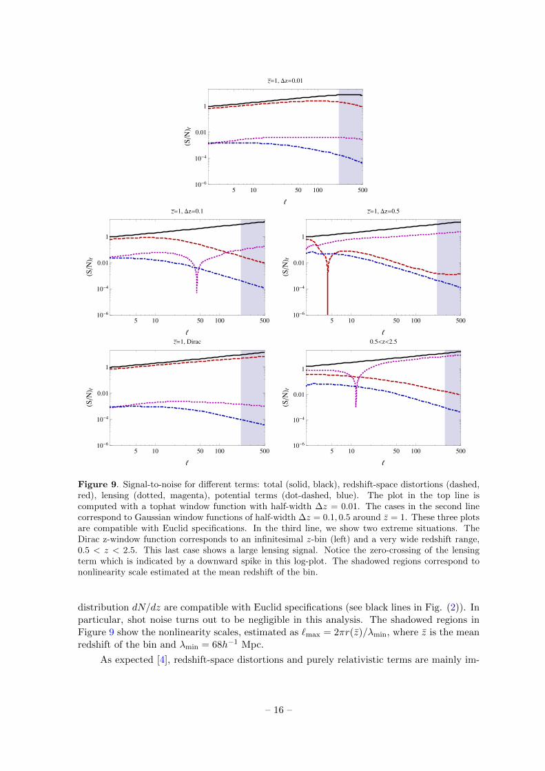
In Figure 9 we show the signal-to-noise for different width of the redshift window func-tion. We consider a tophat window for the narrowest case, ∆z = 0.01 and Gaussian windowfunctions with standard deviations ∆z & 0.05(1 + z), which corresponds to Euclid photo-metric errors [24] for the panels on the second line. The sky fraction, fsky, and the galaxy
– 15 –
5 10 50 100 50010-6
10-4
0.01
1
HSN
L
z=1, Dz=0.01
5 10 50 100 50010-6
10-4
0.01
1
HSN
L
z=1, Dz=0.1
5 10 50 100 50010-6
10-4
0.01
1
HSN
L
z=1, Dz=0.5
5 10 50 100 50010-6
10-4
0.01
1
HSN
L
z=1, Dirac
5 10 50 100 50010-6
10-4
0.01
1
HSN
L
0.5<z<2.5
Figure 9. Signal-to-noise for different terms: total (solid, black), redshift-space distortions (dashed,red), lensing (dotted, magenta), potential terms (dot-dashed, blue). The plot in the top line iscomputed with a tophat window function with half-width ∆z = 0.01. The cases in the second linecorrespond to Gaussian window functions of half-width ∆z = 0.1, 0.5 around z = 1. These three plotsare compatible with Euclid specifications. In the third line, we show two extreme situations. TheDirac z-window function corresponds to an infinitesimal z-bin (left) and a very wide redshift range,0.5 < z < 2.5. This last case shows a large lensing signal. Notice the zero-crossing of the lensingterm which is indicated by a downward spike in this log-plot. The shadowed regions correspond tononlinearity scale estimated at the mean redshift of the bin.
distribution dN/dz are compatible with Euclid specifications (see black lines in Fig. (2)). Inparticular, shot noise turns out to be negligible in this analysis. The shadowed regions inFigure 9 show the nonlinearity scales, estimated as `max = 2πr(z)/λmin, where z is the meanredshift of the bin and λmin = 68h−1 Mpc.
As expected [4], redshift-space distortions and purely relativistic terms are mainly im-
– 16 –
portant at large scales, while lensing has a weaker scale dependence. For small ∆z, apartfrom the usual density term, redshift-space distortions are the main contribution. Theirsignal-to-noise is larger than one, which allows to constrain the growth factor. As ∆z in-creases, redshift-space distortions are washed out, and their signal decreases significantly.On the other hand, lensing and potential terms increase. This is due to the fact that theseterms depend on integrals over z that coherently grow as the width of the z-window functionincreases. While potential terms always remain sub-dominant, the lensing signal-to-noisebecomes larger than 1 for the value of ∆z = 0.5 already at ` ≈ 60.
As a reference, we also show the signal-to-noise for an infinitesimal bin width (Diracz-window function). This corresponds to the largest possible C` amplitude. As in the case∆z = 0.01, redshift-space distortion is of the same order as the density term. Note , however,that in reality for very narrow bins, shot noise becomes important and decreases (S/N)`,especially for large multipoles.
The case of a uniform galaxy distribution between 0.5 < z < 2.5 is also shown. Weassume fsky = 1 and neglect shot noise. In this configuration the lensing term has a very largesignal-to-noise. This can be used to constrain the lensing potential by comparing the observ-able (total) C`’s to the theoretical models. In practice one may adapt this study to catalogsof radio galaxies, which usually cover wide z ranges but with poor redshift determinationwhich is not needed for this case, for previous studies see, e.g., [32–34].
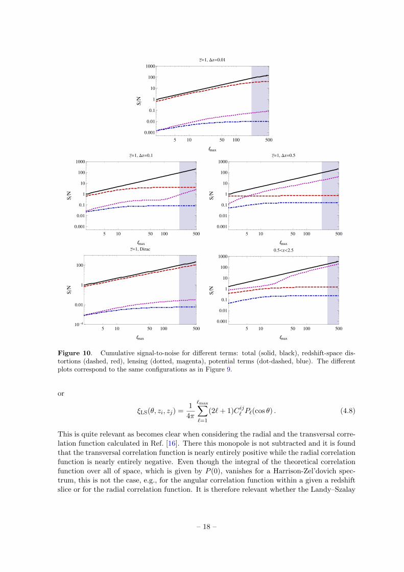
In Figure 10 the cumulative signal-to-noise, Eq. (4.6), is shown as function of themaximum multipole considered in the sum. Contrary to all the other terms, the cumulativesignal-to-noise of the potential terms never exceeds 1. We therefore conclude that the consid-ered experiment is not able to measure the potential terms. It is not clear, whether anotherfeasible configuration would be sensitive to them. Notice also how the lensing term really’kicks in’ after the zero-crossing, when it is not longer dominated by its anti-correlation withthe density term but by the contribution from the autocorrelation.
4.4 The correlation function and the monopole
So far we have not considered the observed monopole, Cij0 , and dipole, Cij1 , since the formeris affected by the value of the gravitational potential and the density fluctuation at theobserver position, while the latter depends on the observer velocity. These quantities are notof interest for cosmology and cannot be determined within linear perturbation theory.
However, there is an additional point which has to be taken into account when con-sidering the correlation function. Usually, the correlation function is determined from anobserved sample of galaxies by subtracting from the number of pairs with given redshiftsand angular separation the corresponding number for a synthetic, uncorrelated sample withthe same observational characteristics (survey geometry, redshift distribution, etc.). This isthe basis of the widely used Landy–Szalay estimator for the determination of the correlationfunction from an observed catalogue of galaxies [35]. For this estimator, by construction, theintegral over angles vanishes, so that
C(LS)0 (zi, zj) = 2π
∫ξLS(θ, zi, zj) sin θdθ = 0 . (4.7)
Here ξLS(θ, zi, zj) is already convolved with the redshift window function of the survey. If wewant to compute the Landy–Szalay estimator for the correlation function we therefore haveto subtract the monopole,
ξLS(θ, zi, zj) = ξ(θ, zi, zj)−1
4πCij0 ,
– 17 –
5 10 50 100 500
0.001
0.01
0.1
1
10
100
1000
max
SN
z=1, Dz=0.01
5 10 50 100 500
0.001
0.01
0.1
1
10
100
1000
max
SN
z=1, Dz=0.1
5 10 50 100 500
0.001
0.01
0.1
1
10
100
1000
max
SN
z=1, Dz=0.5
5 10 50 100 50010-4
0.01
1
100
max
SN
z=1, Dirac
5 10 50 100 500
0.001
0.01
0.1
1
10
100
1000
max
SN
0.5<z<2.5
Figure 10. Cumulative signal-to-noise for different terms: total (solid, black), redshift-space dis-tortions (dashed, red), lensing (dotted, magenta), potential terms (dot-dashed, blue). The differentplots correspond to the same configurations as in Figure 9.
or
ξLS(θ, zi, zj) =1
4π
`max∑`=1
(2`+ 1)Cij` P`(cos θ) . (4.8)
This is quite relevant as becomes clear when considering the radial and the transversal corre-lation function calculated in Ref. [16]. There this monopole is not subtracted and it is foundthat the transversal correlation function is nearly entirely positive while the radial correlationfunction is nearly entirely negative. Even though the integral of the theoretical correlationfunction over all of space, which is given by P (0), vanishes for a Harrison-Zel’dovich spec-trum, this is not the case, e.g., for the angular correlation function within a given a redshiftslice or for the radial correlation function. It is therefore relevant whether the Landy–Szalay
– 18 –
0.00 0.02 0.04 0.06 0.08 0.10
-3
-2
-1
0
1
2
∆z
C=
0Hz,∆
zL1
05
0.00 0.02 0.04 0.06 0.08 0.100
10
20
30
40
50
∆z
MHz,∆
zL1
05
0.00 0.02 0.04 0.06 0.08 0.10
-0.005
-0.004
-0.003
-0.002
-0.001
0.000
0.001
0.002
∆z
ΞHz,∆
zL
0 2 4 6 8
0.000
0.001
0.002
0.003
0.004
0.005
0.006
Θ @degDΞ
Hz,ΘL
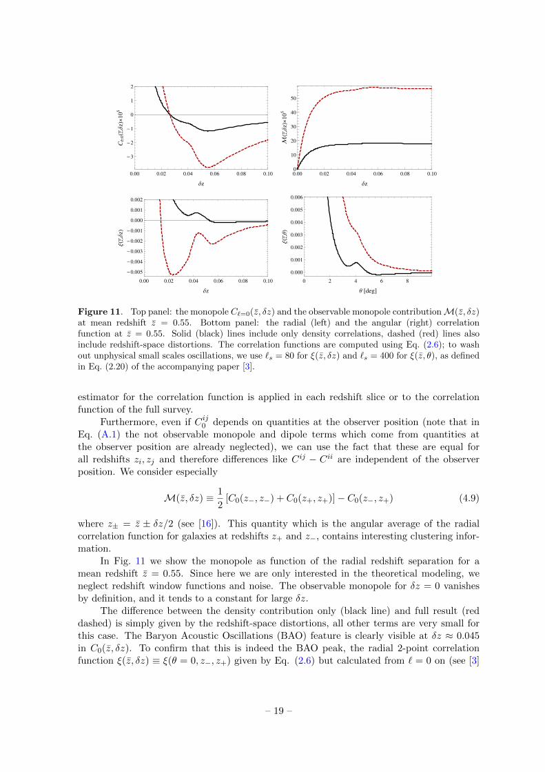
Figure 11. Top panel: the monopole C`=0(z, δz) and the observable monopole contributionM(z, δz)at mean redshift z = 0.55. Bottom panel: the radial (left) and the angular (right) correlationfunction at z = 0.55. Solid (black) lines include only density correlations, dashed (red) lines alsoinclude redshift-space distortions. The correlation functions are computed using Eq. (2.6); to washout unphysical small scales oscillations, we use `s = 80 for ξ(z, δz) and `s = 400 for ξ(z, θ), as definedin Eq. (2.20) of the accompanying paper [3].
estimator for the correlation function is applied in each redshift slice or to the correlationfunction of the full survey.
Furthermore, even if Cij0 depends on quantities at the observer position (note that inEq. (A.1) the not observable monopole and dipole terms which come from quantities atthe observer position are already neglected), we can use the fact that these are equal forall redshifts zi, zj and therefore differences like Cij − Cii are independent of the observerposition. We consider especially
M(z, δz) ≡ 1
2[C0(z−, z−) + C0(z+, z+)]− C0(z−, z+) (4.9)
where z± = z ± δz/2 (see [16]). This quantity which is the angular average of the radialcorrelation function for galaxies at redshifts z+ and z−, contains interesting clustering infor-mation.
In Fig. 11 we show the monopole as function of the radial redshift separation for amean redshift z = 0.55. Since here we are only interested in the theoretical modeling, weneglect redshift window functions and noise. The observable monopole for δz = 0 vanishesby definition, and it tends to a constant for large δz.
The difference between the density contribution only (black line) and full result (reddashed) is simply given by the redshift-space distortions, all other terms are very small forthis case. The Baryon Acoustic Oscillations (BAO) feature is clearly visible at δz ≈ 0.045in C0(z, δz). To confirm that this is indeed the BAO peak, the radial 2-point correlationfunction ξ(z, δz) ≡ ξ(θ = 0, z−, z+) given by Eq. (2.6) but calculated from ` = 0 on (see [3]
– 19 –
for more details) is also shown, presenting the same bump. A detailed study of the BAO peakin the angular power spectrum is left for future work. For completeness, also the transverseangular correlation function ξ(z, θ) ≡ ξ(θ, z, z) is plotted, which shows the BAO peak atθ ≈ 4. Contrary to the radial case in which the BAO scales have negative correlation, thetransverse function is always positive on these scales.
Since we neglect shot noise and assume total sky coverage, cosmic variance from Eq. (4.5),σ`=0 =
√2C`=0(z, δz) leads to a signal-to-noise(
S
N
)`=0
=C`=0(z, δz)
σ`=0=
1√2< 1,
for one given redshift difference δz. This is also approximately the (S/N) for M for largeenough δz. Hence, if we add M(z, δz) for several only weakly correlated redshifts we easilyobtain a measurable signal with S/N > 1.
5 Conclusions
We have shown how the new code classgal [3] can be used to analyze galaxy surveys in anoptimal way. With a few examples we have shown that the figure of merit from an analysisof the C`(z, z
′) spectra can be significantly larger, up to a factor of a few, than the one froma standard P (k) analysis. This is due to the fact that this analysis makes optimal use ofthe redshift information and does not average over directions. Clearly, in the analysis ofupcoming high quality surveys we will want to use this promising method.
We have also seen that the nonlinearity scale, the scale beyond which we can no longertrust the theoretically calculated spectrum, is of uttermost importance for the precision withwhich we estimate cosmological parameters. Within our conservative approach, and LSSdata alone, cosmological parameters cannot be obtained with good precision, see Fig. 4.However, we hope that in the final data analysis we shall have accurate matter power spectradown to significantly smaller scales from N-body or approximation techniques. Furthermore,for an optimal determination of cosmological parameters, we shall of course combine LSSobservations with CMB experiments, e.g. from Planck, and other cosmological data. As wehave seen, the FoM of spectroscopic surveys increases significantly with the number of bins.However, the computational effort scales like N2
bin and thus becomes correspondingly large.Nevertheless, the pre-factor in front of the scaling can be substantially smaller than one whenwe include only cross-correlations from bins within a given spatial distance.
We have also shown that deep angular galaxy catalogs can actually be used to measurethe lensing potential. This is a novel method, alternative to the traditional lensing surveys,which can be used, e.g., to constrain modified gravity theories.
Since the power spectra of galaxy surveys depend on redshift, contrary to the CMB, herealso the monopole contains cosmological information which can in principle be measured.
Acknowledgments
We thank Camille Bonvin, Enrique Gaztanaga, Anaıs Rassat and Alexandre Refregier forhelpful discussions. This work is supported by the Swiss National Science Foundation. RDacknowledges partial support from the (US) National Science Foundation under Grant No.NSF PHY11-25915.
– 20 –
A The galaxy number power spectrum
The galaxy number counts in direction n at observed redshift z are given by [3, 4]
∆(n, z) = D +
[1
H∂r(V · n) +
(H′
H2+
2
r(z)H
)V · n− 3HV
]+
1
r(z)
∫ r(z)
0dr
[2− r(z)− r
r∆Ω
](Φ + Ψ)
+
(H′
H2+
2
r(z)H+ 1
)Ψ
+1
HΦ′ − 2Φ +
(H′
H2+
2
r(z)H
)(Ψ +
∫ r(z)
0dr(Φ′ + Ψ′)
), (A.1)
where V is the potential velocity defined through V = −∇V . Here primes denote derivativesw.r.t. conformal time and the notation agrees with [3]. The first term is the density term,the term in square brackets is the redshift space distortion and the first term on the secondline is the lensing term. The remaining gravitational potential contributions are sometimesalso called “relativistic terms”.
The C`’s from this expression contain not only the auto-correlations of each term butalso their cross-correlation with other contributions. We call the auto-correlation of thedensity term Cδ` (z, z′), the density term; the cross-correlation of density and velocity and theauto-correlation of the velocity term Cz` (z, z′), the redshift space distortion term, the cross-correlation of the lensing contribution with density and velocity and its auto-correlationC lens` (z, z′), the lensing term. We call the rest the ”potential terms”, Cpot
` (z, z′). If the cross-correlation terms dominate, any of these spectra except Cδ` can in principle be negative evenfor z = z′. These are the definitions of the parts of the full angular power spectra which areused in Section 4.3. More details on how these spectra are calculated can be found in theaccompanying paper [3].
B Basics of Fisher matrix forecasts
The Fisher matrix is defined as the derivative of the logarithm of the likelihood with respectto pairs of model parameters. Assuming that the spectra Cij` are Gaussian (which is not agood assumption for small ` but becomes reasonable for ` & 20), the Fisher matrix is givenby (cf. [1, 36])
Fαβ =∑ ∂Cij`
∂λα
∂Cpq`∂λβ
Cov−1`,(ij),(pq), (B.1)
where λα denotes the different cosmological parameters we want to constrain. The sum over` runs from 2 to a value `max related to the non-linearity scale kmax: we discuss this issuein section 3.2. Note also that we sum over the matrix indices (ij) with i ≤ j and (pq) withp ≤ q which run from 1 to Nbin .
In the Fisher matrix approximation, i.e. assuming that the likelihood is a multivariateGaussian with respect to cosmological parameters (which usually is not the case), the regionin the full parameter space corresponding to a given Confidence Level (CL) is an ellipsoidcentered on the best-fit model with parameters λα, with boundaries given by the equation∑
α,β(λα− λα)(λβ− λβ)Fαβ = [∆χ2]5, and with a volume given (up to a numerical factor) by
5The number ∆χ2 depends both on the requested confidence level and on the number n of parameters: forn = 1 (resp. 2) and a 68%CL one should use ∆χ2 = 1 (resp. 2.3). For other values see section 15.6 of [37].
– 21 –
[det(F−1)]1/2 (see e.g. [1]). Since the smallness of this volume is a measure of the performanceof a given experiment, one often uses the inverse of the square root of the determinant as aFigure of merit,
FoM =[det(F−1
)]−1/2.
If we assume several parameters to be fixed by external measurements at the best-fit valueλα, the 1σ ellipsoid for the remaining parameters is given by the same equation, but with thesum running only over the remaining parameters. Hence the volume of this ellipsoid is givenby the square root of the determinant of the sub-matrix of F restricted to the remainingparameters, that we call F . In that case, the FoM for measuring the remaining parametersreads
FoMfixed =[det(
(F )−1)]−1/2
.
However, it is often relevant to evaluate how well one (or a few) parameters can be measuredwhen the other parameters are marginalized over. In this case, a few lines of calculationshow that the figure of merit is given by taking the sub-matrix of the inverse, instead of theinverse of the sub-matrix (see [1]),
FoMmarg. =[det(F−1
)]−1/2.
In particular, if we are interested in a single parameter λα and assume that all other param-eters are marginalized over, the FoM for measuring λα is given by
FoMmarg. =[(F−1)αα
]−1/2.
When the likelihood is not a multivariate Gaussian with respect to cosmological parameters,the 68% CL region is no longer an ellipsoid, but the FoM given above (with the Fisher matrixbeing evaluated at the best-fit point) usually remains a good indicator.
It is however possible to construct examples where the FoM estimate completely fails.For instance, if two parameters are degenerate in a such a way that their profile likelihoodis strongly non-elliptical (e.g. with a thin and elongated banana shape). Then Fisher-basedFoM will rely on a wrong estimate of the surface of the banana, and will return a very poorapproximation of the true FoM. This happens e.g. when including isocurvature modes [38],for mixed dark matter models [39] or in some modified gravity models [40].
For the power spectrum analysis, following [41, 42], we define the Fisher matrix in eachredshift bin as
Fαβ=
∫ 1
−1
∫ kmax
kmin
∂ lnPobs
∂λα
∂ lnPobs
∂λβVeff
k2dkdµ
2(2π)2, (B.2)
where the effective volume Veff is related to the actual volume Vbin of each redshift bin through
Veff(k, µ, z) =
[Pobs(k, µ, z)
Pobs(k, µ, z) + 1/n(z)
]2
Vbin(z) . (B.3)
Here z is the mean redshift of the bin, and n(z) the average galaxy density in this bin,assumed to be uniform over the sky. In the case of several non-overlapping z-bins, we assumethat measurements inside each of them are independent so that the total Fisher matrix isthe sum of those computed for every bin. This expression is in principle valid in the flat-sky approximation. However, since it encodes all the statistical information, we can use it
– 22 –
for a forecast analysis. The denominator in Eq. (B.3) features the two contributions to thevariance of the observable power spectrum Pobs(k, µ, z) coming from sampling variance andfrom shot noise. The observable power spectrum Pobs(k, µ, z) (not including shot noise) isgiven in the minimal ΛCDM (Λ Cold Dark Matter) model by the theoretical power spectrumP (k) calculated at z = 0, rescaled according to
Pobs(k, µ, z) =DA(z)2H(z)
DA(z)2H(z)
(1 + µ2ΩM (z)γ
)2G(z)2P (k) . (B.4)
The first ratio in Eq. (B.4) takes in account the volume difference for different cosmologies.The survey volume for galaxies in a redshift bin centered on z and of width δz is proportionalto DA(z)2H(z)−1δz. The quantities DA and H are evaluated at the fiducial cosmology.The parenthesis contains the Kaiser approximation to redshift-space distortions [17], whichtogether with the density term is the dominant contribution in Eq. (A.1) for our analysis.We assume an exponent γ = 0.6 that is a good approximation to the growth factor fromlinear perturbation theory in ΛCDM. We have neglected the bias (b = 1) in order to comparethe results with the FoM derived from the angular power spectrum C`(z1, z2) where we alsoset b = 1. When we consider photometric redshift surveys, we need take into account theloss of information in the longitudinal direction due to the redshift error σz. Following [42],
we then multiply Pobs(k, µ, z) with an exponential cutoff e−(kµσz/H(z))2
.In Eq. (B.2), the observable power spectrum and the effective volume are assumed to
be expressed in Hubble-rescaled units, e.g [Mpc/h]3, while wave numbers are expressed inunits of [h/Mpc]. In other words, it would be more rigorous to write everywhere ([a3
0H30Pobs],
[k/(a0H0)], [a30H
30Veff ]) instead of (Pobs, k, Veff): the quantities in brackets are the dimension-
less numbers that are actually measured, see [43]. Using Hubble-rescaled units does make adifference in the calculation of the partial derivative with respect to the model parameter H0:it is important to keep k/h and not k constant. Also, the wavenumber kmax correspondingto the non-linearity scale is given in units h/Mpc, so that we fix kmax/h.
Furthermore, since the computation of P (k) involves the assumption of a cosmologicalmodel to convert observable angles and redshifts into distances, expressing the latter inMpc/h mitigates the uncertainty introduced in this procedure since, to first approximation,distances r(z) =
∫dz/H(z) scale as h−1.
References
[1] R. Durrer, The Cosmic Microwave Background. Cambridge University Press, Cambridge, UK,2008.
[2] Planck Collaboration Collaboration, P. Ade et al., Planck 2013 results. XVI. Cosmologicalparameters, arXiv:1303.5076.
[3] E. Di Dio, F. Montanari, J. Lesgourgues, and R. Durrer, The CLASSgal code for RelativisticCosmological Large Scale Structure, JCAP 1311 (2013) 044, [arXiv:1307.1459].
[4] C. Bonvin and R. Durrer, What galaxy surveys really measure, Phys.Rev. D84 (2011) 063505,[arXiv:1105.5280].
[5] A. Challinor and A. Lewis, The linear power spectrum of observed source number counts,Phys.Rev. D84 (2011) 043516, [arXiv:1105.5292].
[6] J. Yoo, A. L. Fitzpatrick, and M. Zaldarriaga, A New Perspective on Galaxy Clustering as aCosmological Probe: General Relativistic Effects, Phys.Rev. D80 (2009) 083514,[arXiv:0907.0707].
– 23 –
[7] J. Yoo, General Relativistic Description of the Observed Galaxy Power Spectrum: Do WeUnderstand What We Measure?, Phys.Rev. D82 (2010) 083508, [arXiv:1009.3021].
[8] D. Jeong, F. Schmidt, and C. M. Hirata, Large-scale clustering of galaxies in general relativity,Phys.Rev. D85 (2012) 023504, [arXiv:1107.5427].
[9] F. Schmidt and D. Jeong, Cosmic Rulers, Phys.Rev. D86 (2012) 083527, [arXiv:1204.3625].
[10] D. Bertacca, R. Maartens, A. Raccanelli, and C. Clarkson, Beyond the plane-parallel andNewtonian approach: Wide-angle redshift distortions and convergence in general relativity,JCAP 1210 (2012) 025, [arXiv:1205.5221].
[11] D. Jeong and F. Schmidt, Cosmic Clocks, Phys.Rev. D89 (2014) 043519, [arXiv:1305.1299].
[12] C. Blake, K. Glazebrook, T. Davis, S. Brough, M. Colless, et al., The WiggleZ Dark EnergySurvey: measuring the cosmic expansion history using the Alcock-Paczynski test and distantsupernovae, Mon.Not.Roy.Astron.Soc. 418 (2011) 1725–1735, [arXiv:1108.2637].
[13] B. A. Reid, L. Samushia, M. White, W. J. Percival, M. Manera, et al., The clustering ofgalaxies in the SDSS-III Baryon Oscillation Spectroscopic Survey: measurements of the growthof structure and expansion rate at z=0.57 from anisotropic clustering, arXiv:1203.6641.
[14] S. Nuza, A. Sanchez, F. Prada, A. Klypin, D. Schlegel, et al., The clustering of galaxies at z 0.5in the SDSS-III Data Release 9 BOSS-CMASS sample: a test for the LCDM cosmology,Mon.Not.Roy.Astron.Soc. 432 (2013) 743–760, [arXiv:1202.6057].
[15] L. Anderson, E. Aubourg, S. Bailey, F. Beutler, A. S. Bolton, et al., The clustering of galaxiesin the SDSS-III Baryon Oscillation Spectroscopic Survey: Measuring DA and H at z=0.57 fromthe Baryon Acoustic Peak in the Data Release 9 Spectroscopic Galaxy Sample,arXiv:1303.4666.
[16] F. Montanari and R. Durrer, A new method for the Alcock-Paczynski test, Phys.Rev. D86(2012) 063503, [arXiv:1206.3545].
[17] N. Kaiser, Clustering in real space and in redshift space, Mon.Not.Roy.Astron.Soc. 227 (July,1987) 1–21.
[18] A. J. S. Hamilton, Measuring Omega and the real correlation function from the redshiftcorrelation function, Astrophys.J. 385 (Jan., 1992) L5–L8.
[19] A. Raccanelli, L. Samushia, and W. J. Percival, Simulating redshift-space distortions for galaxypairs with wide angular separation, Mon.Not.Roy.Astron.Soc. 409 (2010), no. 4 1525–1533.
[20] C. Carbone, O. Mena, and L. Verde, Cosmological Parameters Degeneracies and Non-GaussianHalo Bias, JCAP 1007 (2010) 020, [arXiv:1003.0456].
[21] V. Desjacques, Local bias approach to the clustering of discrete density peaks, Phys.Rev. D87(2013), no. 4 043505, [arXiv:1211.4128].
[22] J. Asorey, M. Crocce, E. Gaztanaga, and A. Lewis, Recovering 3D clustering information withangular correlations, Mon.Not.Roy.Astron.Soc. 427 (2012), no. 3 1891–1902,[arXiv:1207.6487].
[23] B. Audren, J. Lesgourgues, S. Bird, M. G. Haehnelt, and M. Viel, Neutrino masses andcosmological parameters from a Euclid-like survey: Markov Chain Monte Carlo forecastsincluding theoretical errors, JCAP 1301 (2013) 026, [arXiv:1210.2194].
[24] EUCLID Collaboration Collaboration, R. Laureijs et al., Euclid Definition Study Report,arXiv:1110.3193.
[25] J. Asorey, M. Crocce, and E. Gaztanaga, Redshift-space distortions from the cross-correlationof photometric populations, arXiv:1305.0934.
– 24 –
[26] N. P. Ross, J. da Angela, T. Shanks, D. A. Wake, R. D. Cannon, et al., The 2dF-SDSS LRGand QSO Survey: The 2-Point Correlation Function and Redshift-Space Distortions,Mon.Not.Roy.Astron.Soc. 381 (2007) 573–588, [astro-ph/0612400].
[27] WiggleZ Collaboration Collaboration, C. Contreras et al., The WiggleZ Dark EnergySurvey: measuring the cosmic growth rate with the two-point galaxy correlation function,Mon.Not.Roy.Astron.Soc. 430 (Aprile, 2013) 924–933, [arXiv:1302.5178].
[28] S. de la Torre, L. Guzzo, J. Peacock, E. Branchini, A. Iovino, et al., The VIMOS PublicExtragalactic Redshift Survey (VIPERS). Galaxy clustering and redshift-space distortions atz=0.8 in the first data release, arXiv:1303.2622.
[29] S. Asaba, C. Hikage, K. Koyama, G.-B. Zhao, A. Hojjati, et al., Principal Component Analysisof Modified Gravity using Weak Lensing and Peculiar Velocity Measurements, JCAP 1308(2013) 029, [arXiv:1306.2546].
[30] I. D. Saltas and M. Kunz, Anisotropic stress and stability in modified gravity models, Phys.Rev.D83 (2011) 064042, [arXiv:1012.3171].
[31] R. Durrer and R. Maartens, Dark Energy and Dark Gravity, Gen.Rel.Grav. 40 (2008) 301–328,[arXiv:0711.0077].
[32] C. Blake, T. Mauch, and E. M. Sadler, Angular clustering in the SUMSS radio survey,Mon.Not.Roy.Astron.Soc. 347 (2004) 787, [astro-ph/0310115].
[33] M. Negrello, F. Perrotta, J. G.-N. Gonzalez, L. Silva, G. De Zotti, et al., Astrophysical andCosmological Information from Large-scale sub-mm Surveys of Extragalactic Sources,Mon.Not.Roy.Astron.Soc. 377 (2007) 1557–1568, [astro-ph/0703210].
[34] R. Subrahmanyan, R. Ekers, L. Saripalli, and E. Sadler, A deep survey of thelow-surface-brightness radio sky, PoS MRU (2007) 055, [arXiv:0802.0053].
[35] S. D. Landy and A. S. Szalay, Bias and variance of angular correlation functions, Astrophys.J.412 (1993) 64–71.
[36] L. Verde, Statistical methods in cosmology, Lect.Notes Phys. 800 (2010) 147–177,[arXiv:0911.3105].
[37] W. H. Press, S. A. Teukolsky, W. T. Vetterling, and B. P. Flannery, Numerical Recipes 3rdEdition: The Art of Scientific Computing. Cambridge University Press, Cambridge, UK, 2007.
[38] Planck Collaboration Collaboration, P. Ade et al., Planck 2013 results. XXII. Constraintson inflation, arXiv:1303.5082.
[39] A. Boyarsky, J. Lesgourgues, O. Ruchayskiy, and M. Viel, Lyman-alpha constraints on warmand on warm-plus-cold dark matter models, JCAP 0905 (2009) 012, [arXiv:0812.0010].
[40] B. Audren, D. Blas, J. Lesgourgues, and S. Sibiryakov, Cosmological constraints on Lorentzviolating dark energy, JCAP 1308 (2013) 039, [arXiv:1305.0009].
[41] M. Tegmark, Measuring cosmological parameters with galaxy surveys, Phys.Rev.Lett. 79 (1997)3806–3809, [astro-ph/9706198].
[42] H.-J. Seo and D. J. Eisenstein, Probing dark energy with baryonic acoustic oscillations fromfuture large galaxy redshift surveys, Astrophys.J. 598 (2003) 720–740, [astro-ph/0307460].
[43] J. Lesgourgues, G. Mangano, G. Miele, and S. Pastor, Neutrino Cosmology. CambridgeUniversity Press, Cambridge, UK, Feb., 2013.
– 25 –